value streams from distribution grid support using utility ... · sumitomo electric usa (seusa)...
TRANSCRIPT

NREL is a national laboratory of the U.S. Department of Energy Office of Energy Efficiency & Renewable Energy Operated by the Alliance for Sustainable Energy, LLC
This report is available at no cost from the National Renewable Energy Laboratory (NREL) at www.nrel.gov/publications.
Contract No. DE-AC36-08GO28308
Value Streams from Distribution Grid Support Using Utility-Scale Vanadium Redox Flow Battery NREL-Sumitomo Electric Battery Demonstration Project
Adarsh Nagarajan, Dylan Cutler, Aadil Latif, Xiangkun Li, Richard Bryce, Ying Shi, Jin Tan, Qian Long, Peter Gotseff, Ershun Du, and Murali Baggu National Renewable Energy Laboratory
Yoshihiro Hirata, Katsuya Yamanishi, Keiji Yano, Riichi Kitano, and Yoshiyuki Nagaoka Sumitomo Electric USA (SEUSA)
Technical Report NREL/TP-5D00-71545 August 2018

NREL is a national laboratory of the U.S. Department of Energy Office of Energy Efficiency & Renewable Energy Operated by the Alliance for Sustainable Energy, LLC
This report is available at no cost from the National Renewable Energy Laboratory (NREL) at www.nrel.gov/publications.
Contract No. DE-AC36-08GO28308
National Renewable Energy Laboratory 15013 Denver West Parkway Golden, CO 80401 303-275-3000 • www.nrel.gov
Value Streams from Distribution Grid Support Using Utility-Scale Vanadium Redox Flow Battery NREL-Sumitomo Electric Battery Demonstration Project Adarsh Nagarajan, Dylan Cutler, Aadil Latif, Xiangkun Li, Richard Bryce, Ying Shi, Jin Tan, Qian Long, Peter Gotseff, Ershun Du, and Murali Baggu National Renewable Energy Laboratory
Yoshihiro Hirata, Katsuya Yamanishi, Keiji Yano, Riichi Kitano, and Yoshiyuki Nagaoka Sumitomo Electric USA (SEUSA)
Technical Report NREL/TP-5D00-71545 August 2018

iii This report is available at no cost from the National Renewable Energy Laboratory (NREL) at www.nrel.gov/publications.
NOTICE
This work was authored in part by the National Renewable Energy Laboratory (NREL), operated by Alliance for Sustainable Energy, LLC, for the U.S. Department of Energy (DOE) under Contract No. DE-AC36-08GO28308. Funding provided by the New Energy and Industrial Technology Development Organization (NEDO) and Sumitomo Electric. This work is based on results obtained from a project commissioned by the New Energy and Industrial Technology Development Organization (NEDO). The views expressed in the article do not necessarily represent the views of the DOE or the U.S. Government. SDG&E does not prescribe to all the values stream NREL has assigned in this report. The economic conclusions arrived to by NREL and NREL only.
This report is available at no cost from the National Renewable Energy Laboratory (NREL) at www.nrel.gov/publications.
U.S. Department of Energy (DOE) reports produced after 1991 and a growing number of pre-1991 documents are available free via www.OSTI.gov.
Cover Photos by Dennis Schroeder: (left to right) NREL 26173, NREL 18302, NREL 19758, NREL 29642, NREL 19795.
NREL prints on paper that contains recycled content.

iv This report is available at no cost from the National Renewable Energy Laboratory (NREL) at www.nrel.gov/publications.
List of Acronyms ANN Artificial neural network BLAST Battery Lifetime Analysis and Simulation Tool CAISO California Independent System Operator CSV Comma Separated Value DoY Day of year HRRR High-Resolution Rapid Refresh LFP Lithium iron phosphate/graphite LIB Lithium-ion battery Li-ion Lithium-ion LMP Locational marginal price LTC Load tap changer NCA Lithium nickel cobalt aluminum oxide/graphite NGR Non-generator resource NMC Lithium nickel manganese cobalt oxide/graphite NREL National Renewable Energy Laboratory O&M Operation and maintenance PCS Power conditioning system PDR Proxy demand resource PG Participating generator PL Participating load PS Participating system PV Photovoltaic RDRR Reliability demand response resource REM Regulation Energy Management REopt Renewable Energy Integration and Optimization RMSE Root mean square error SDG&E San Diego Gas & Electric Company SOC State of charge VAR Volt-ampere reactive VRFB Vanadium redox flow battery WDAT Wholesale distribution access tariff WDT Wholesale distribution tariff XML Extensible Markup Language

v This report is available at no cost from the National Renewable Energy Laboratory (NREL) at www.nrel.gov/publications.
Executive Summary The National Renewable Energy Laboratory (NREL) collaborated with Sumitomo Electric to provide research support in modeling and optimally dispatching a utility-scale vanadium redox flow battery (VRFB) energy storage system. The primary objective of the project was to identify value streams through the application of utility-scale VRFB for local grid support use cases, including:
• Voltage regulation (droop): When operated in this mode, the system maintains the voltage on the feeder close to its nominal value. To accomplish this objective, the reactive power dispatched from the VRFB is based on the voltage at the battery’s point of common coupling using a voltage droop curve.
• Capacity firming: In this mode, the VRFB smooths high-frequency power flow fluctuations at the substation to a constant or low-frequency timescale average value.
• Peak shaving and valley filling: Peak shaving is defined as displacing the power consumption of the feeder by a predetermined amount for a specific time; this is a special case of load shifting. In this control mode, the VRFB is used to regulate the peak power of the feeder within a predefined limit.
• Energy arbitrage: To take advantage of the price difference of electricity across time periods, the VRFB is charged during off-peak hours and discharged during peak hours. The revenue obtained is the price differential between buying and selling electrical energy minus the cost of losses during the full charge/discharge cycle.
This project was also supported by San Diego Gas & Electric Company (SDG&E). SDG&E provided data and approval to operate their VRFB energy storage system on an SDG&E distribution feeder. NREL worked with Sumitomo Electric to evaluate optimal dispatch strategies to VRFB, analyze the technical impacts, and calculate the associated cost-benefit ratio of substation-level energy storage on an SDG&E distribution feeder.
To support this research, NREL evaluated the impacts of the battery use cases suggested by Sumitomo on the SDG&E host feeder. In addition to evaluating the battery use case, this effort identified possible ways to monetize the benefits from distribution feeder support.
Distribution Feeder Under Study
A utility-scale VRFB was commissioned in the distribution feeder on May 2017 at a location shown in Figure ES-1. A portion of the TEST FEEDER feeder between the VRFB and the primary overhead line connecting to the substation (marked ‘S’) is capacity-constrained (Figure 28). This 1.5-mile #6 overhead cable has a maximum rating of 2.25 MVA, and it directly impacts the maximum charging capacity of the VRFB system. Because the VRFB is installed downstream of the capacity-constrained line, total load from that point of the feeder and below (along with VRFB charging power) cannot exceed 2.25 MVA.

vi This report is available at no cost from the National Renewable Energy Laboratory (NREL) at www.nrel.gov/publications.
Figure ES-1. Topology of the distribution feeder highlighting the location of the energy storage
system
Key tasks that were performed included:
• Modeling and simulation of the distribution substation including all seven feeders (detailed test feeder and aggregated loads for the other six feeders).
• Developed and validated the battery control models for voltage regulation, peak shaving/valley filling and capacity firming.
• Assigned costs to distribution feeder support and optimally dispatched the energy storage system.
• Generated optimal battery operation schedules.
• Assessed battery energy storage participation in California Independent System Operator (CAISO) markets.
• Developed an understanding and compared value streams between the VRFB and lithium-ion (Li-ion) battery chemistries.
• Developed high-fidelity loss models for the VRFB.
• Generated load forecasts for one week and performed day-ahead dispatch of the VRFB under test based on CAISO day-ahead price signals.
Following are descriptions of key methodologies and results.
Model the Distribution Substation
The models of the distribution feeders in Synergi (provided by SDG&E) were converted by NREL; i.e. the Synergi files were parsed to generate a feeder model in the OpenDSS format. The converted model was validated for node voltages, and the feeder sequence impedance was

vii This report is available at no cost from the National Renewable Energy Laboratory (NREL) at www.nrel.gov/publications.
compared with the original Synergi models. This task involved running a snapshot simulation in Synergi and OpenDSS for identical loading/photovoltaic levels. The node voltages and sequence impedances were compared between Synergi and OpenDSS. Ultimately, the voltage comparison errors were successfully restricted and sequence impedance comparison errors to a range within 1% of the intended values.
The requisite data provided by SDG&E included annual feeder load data, annual solar irradiance profiles, and VRFB energy storage system charge and discharge rates and limits, such as the monitoring point for power, voltage, frequency, range of state of charge, and range of active/reactive power. Additionally, SDG&E provided the technical specifications data sheets for the inverter and voltage control equipment (e.g., regulators and capacitors).
Develop and Validate VRFB Controls
Control models were developed to simulate the various VRFB use cases (i.e., voltage regulation, peak shaving, and capacity firming) to understand the impacts of the VRFB on local grid support. The simulations were carried out using seasonal load profiles from the year 2016. The aim of this effort was to gain insight on different modes under which the battery can operate. Sumitomo Electric provided the performance characteristics of the VRFB that were needed for detailed modeling and cross-validation for the various use cases. Figure ES-2 shows a comparison between our control model for peak shaving and the field measurements. A similar comparison was performed for capacity firming and voltage regulation, as is detailed later in the report.
Figure ES-2. Comparison of peak-shaving algorithms using the field data
Analyze Value Stream
The economics of using the VRFB to provide grid support functions were evaluated through a combination of OpenDSS simulations and mixed-integer linear programming optimizations using NREL’s Renewable Energy Integration and Optimization (REopt) framework. Figure ES-3
viii This report is available at no cost from the National Renewable Energy Laboratory (NREL) at www.nrel.gov/publications.
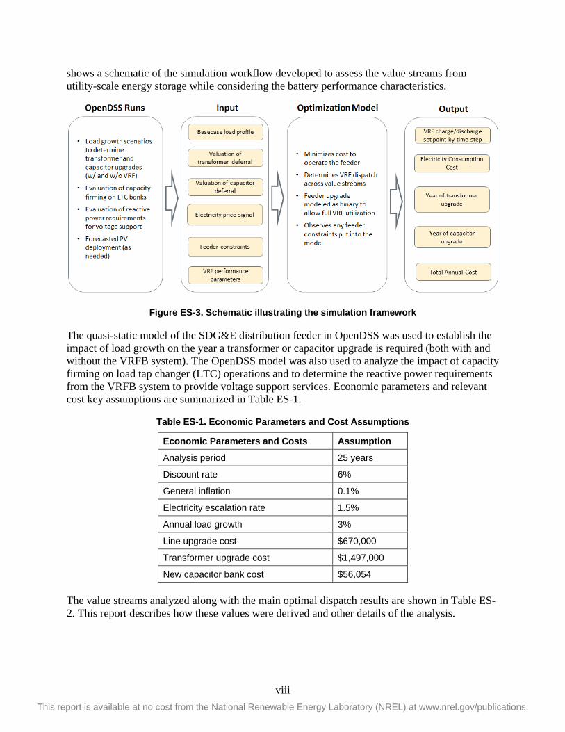
shows a schematic of the simulation workflow developed to assess the value streams from utility-scale energy storage while considering the battery performance characteristics.
Figure ES-3. Schematic illustrating the simulation framework
The quasi-static model of the SDG&E distribution feeder in OpenDSS was used to establish the impact of load growth on the year a transformer or capacitor upgrade is required (both with and without the VRFB system). The OpenDSS model was also used to analyze the impact of capacity firming on load tap changer (LTC) operations and to determine the reactive power requirements from the VRFB system to provide voltage support services. Economic parameters and relevant cost key assumptions are summarized in Table ES-1.
Table ES-1. Economic Parameters and Cost Assumptions
Economic Parameters and Costs Assumption
Analysis period 25 years
Discount rate 6%
General inflation 0.1%
Electricity escalation rate 1.5%
Annual load growth 3%
Line upgrade cost $670,000
Transformer upgrade cost $1,497,000
New capacitor bank cost $56,054
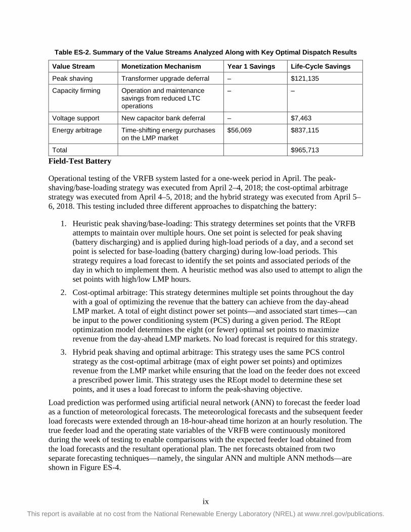
The value streams analyzed along with the main optimal dispatch results are shown in Table ES-2. This report describes how these values were derived and other details of the analysis.
ix This report is available at no cost from the National Renewable Energy Laboratory (NREL) at www.nrel.gov/publications.
Table ES-2. Summary of the Value Streams Analyzed Along with Key Optimal Dispatch Results
Value Stream Monetization Mechanism Year 1 Savings Life-Cycle Savings
Peak shaving Transformer upgrade deferral – $121,135
Capacity firming Operation and maintenance savings from reduced LTC operations
– –
Voltage support New capacitor bank deferral – $7,463
Energy arbitrage Time-shifting energy purchases on the LMP market
$56,069 $837,115
Total
$965,713
Field-Test Battery
Operational testing of the VRFB system lasted for a one-week period in April. The peak-shaving/base-loading strategy was executed from April 2–4, 2018; the cost-optimal arbitrage strategy was executed from April 4–5, 2018; and the hybrid strategy was executed from April 5–6, 2018. This testing included three different approaches to dispatching the battery:
1. Heuristic peak shaving/base-loading: This strategy determines set points that the VRFB attempts to maintain over multiple hours. One set point is selected for peak shaving (battery discharging) and is applied during high-load periods of a day, and a second set point is selected for base-loading (battery charging) during low-load periods. This strategy requires a load forecast to identify the set points and associated periods of the day in which to implement them. A heuristic method was also used to attempt to align the set points with high/low LMP hours.
2. Cost-optimal arbitrage: This strategy determines multiple set points throughout the day with a goal of optimizing the revenue that the battery can achieve from the day-ahead LMP market. A total of eight distinct power set points—and associated start times—can be input to the power conditioning system (PCS) during a given period. The REopt optimization model determines the eight (or fewer) optimal set points to maximize revenue from the day-ahead LMP markets. No load forecast is required for this strategy.
3. Hybrid peak shaving and optimal arbitrage: This strategy uses the same PCS control strategy as the cost-optimal arbitrage (max of eight power set points) and optimizes revenue from the LMP market while ensuring that the load on the feeder does not exceed a prescribed power limit. This strategy uses the REopt model to determine these set points, and it uses a load forecast to inform the peak-shaving objective.
Load prediction was performed using artificial neural network (ANN) to forecast the feeder load as a function of meteorological forecasts. The meteorological forecasts and the subsequent feeder load forecasts were extended through an 18-hour-ahead time horizon at an hourly resolution. The true feeder load and the operating state variables of the VRFB were continuously monitored during the week of testing to enable comparisons with the expected feeder load obtained from the load forecasts and the resultant operational plan. The net forecasts obtained from two separate forecasting techniques—namely, the singular ANN and multiple ANN methods—are shown in Figure ES-4.

x This report is available at no cost from the National Renewable Energy Laboratory (NREL) at www.nrel.gov/publications.
Figure ES-4. Net forecast for the singular ANN and the multiple ANN methods along with the
measured feeder load
The total revenue during the two days of hybrid peak shaving and optimal arbitrage was calculated from the observed data to be $217 (with $192 of that resulting from the first 24 hours, without the peak-shaving constraint). The modeled revenue expected by the model was $223 during the two days. The results show good agreement on both the dispatch of the systems and the achievable revenue generation.
xi This report is available at no cost from the National Renewable Energy Laboratory (NREL) at www.nrel.gov/publications.
Table of Contents 1 Modeling SDG&E Distribution System ............................................................................................... 1
1.1 Synergi-to-OpenDSS Conversion ................................................................................................. 1 1.1.1 Model Conversion ............................................................................................................ 1 1.1.2 OpenDSS Model Verification .......................................................................................... 4 1.1.3 Modeling the Substation with All Feeders ....................................................................... 7
1.2 Battery Model and Details ............................................................................................................. 8 1.2.1 Overview of Battery Characteristics ................................................................................ 8
1.3 Annual Data Analysis .................................................................................................................. 11 1.3.1 Data Processing Description .......................................................................................... 11 1.3.2 Results of Annual Analysis ............................................................................................ 14
2 Modeling Battery Use Cases in Distribution System Simulator .................................................... 18 2.1 Modes of Operation ..................................................................................................................... 18 2.2 Simulation Setup ......................................................................................................................... 18 2.3 Peak Shaving and Capacity Deferral ........................................................................................... 19 2.4 Capacity Firming (Smoothing) .................................................................................................... 24 2.5 Voltage Regulation ...................................................................................................................... 27
3 Energy Storage Value Streams from Distribution Support ............................................................ 30 3.1 Introduction and Background ...................................................................................................... 30 3.2 Value Streams for Distribution Grid Support Monetization ....................................................... 30
3.2.1 Applications Chosen for Distribution Grid Support ....................................................... 30 3.2.2 Distribution Feeder and Substation Conditions .............................................................. 32
3.3 Framework for Value Stream Modeling and Comparison .......................................................... 34 3.3.1 Calculating the Value of Distribution Upgrade Deferral ............................................... 34 3.3.2 Framework for Peak Shaving ......................................................................................... 36 3.3.3 Framework for Capacity Firming ................................................................................... 36 3.3.4 Framework for Voltage Support .................................................................................... 36 3.3.5 Framework for Energy Arbitrage ................................................................................... 37
3.4 REopt Simulation Framework for Identifying Value Streams .................................................... 39 3.4.1 Input Data for Value Stream Analysis ........................................................................... 40 3.4.2 REopt Overview ............................................................................................................. 41 3.4.3 VRFB Loss Modeling in REopt ..................................................................................... 41 3.4.4 Expected Outputs from REopt ....................................................................................... 44
3.5 Value Stream Assessment and Results ........................................................................................ 44 3.5.1 Value Stream from Peak Shaving and Energy Arbitrage ............................................... 44 3.5.2 Value Stream from Capacity Firming ............................................................................ 46 3.5.3 Value Stream from Voltage Support: Capacitor Avoidance Costs ................................ 47 3.5.4 Modeling Shutting Off Auxiliary Pumps when the Battery Is Idle ................................ 51 3.5.5 Value from Line Upgrade Deferral ................................................................................ 52
4 CAISO Market for Energy Storage .................................................................................................... 53 4.1 Introduction ................................................................................................................................. 53
4.1.1 Market Participants ........................................................................................................ 53 4.1.2 Markets in CAISO .......................................................................................................... 53
4.2 Market Participation Model/Resource Model ............................................................................. 54 4.2.1 NGRs .............................................................................................................................. 55 4.2.2 Demand Response Product ............................................................................................. 57
5 Dynamic Efficiency and Dynamic Loss Modeling ........................................................................... 59 5.1 Data Sampling ............................................................................................................................. 59 5.2 Dynamic Efficiency Modeling .................................................................................................... 59 5.3 Dynamic Loss Modeling Techniques .......................................................................................... 62

xii This report is available at no cost from the National Renewable Energy Laboratory (NREL) at www.nrel.gov/publications.
5.3.1 Metrics for Evaluating Model Accuracy ........................................................................ 62 5.3.2 Triangular Interpolation ................................................................................................. 62 5.3.3 Composite Quadratic Fitting .......................................................................................... 63 5.3.4 Bivariate Quadratic Fitting ............................................................................................. 64 5.3.5 Nonlinear ANN Model ................................................................................................... 65 5.3.6 Dynamic Loss Modeling ................................................................................................ 67
5.4 Accuracy Impacts Operation Strategies ...................................................................................... 67 5.4.1 Accuracy Impacts Operation Strategies ......................................................................... 68
6 Operational Planning and Field-Testing .......................................................................................... 75 6.1 Scope of Testing .......................................................................................................................... 75 6.2 ANN Model for Feeder Load Forecasting .................................................................................. 75
6.2.1 Historical Feeder Load Data .......................................................................................... 75 6.2.2 High-Resolution Rapid Refresh Meteorological Data ................................................... 76 6.2.3 Singular ANN Model Training ...................................................................................... 76 6.2.4 Multiple ANN Model Training ...................................................................................... 77 6.2.5 Metrics for Performance Evaluation .............................................................................. 78
6.3 VRFB Dispatch Strategies .......................................................................................................... 78 6.3.1 Operational Constraints .................................................................................................. 78
6.4 Results 79 6.4.1 Load Forecasting Results ............................................................................................... 79 6.4.2 Optimal Dispatch Results ............................................................................................... 81
7 Conclusions and Remarks ................................................................................................................ 84 7.1 Peak Shaving ............................................................................................................................... 85 7.2 Capacity Firming ......................................................................................................................... 85 7.3 Voltage Support ........................................................................................................................... 86 7.4 Energy Arbitrage ......................................................................................................................... 86 7.5 Multiuse ....................................................................................................................................... 86 7.6 Current System Under Consideration .......................................................................................... 86 7.7 Value Streams Monetization Results .......................................................................................... 87 7.8 Field-Testing the Battery ............................................................................................................. 87
References ................................................................................................................................................. 89
xiii This report is available at no cost from the National Renewable Energy Laboratory (NREL) at www.nrel.gov/publications.
List of Figures Figure ES-1. Topology of the distribution feeder highlighting the location of the energy storage system . vi Figure ES-2. Comparison of peak-shaving algorithms using the field data ................................................ vii Figure ES-3. Schematic illustrating the simulation framework ................................................................. viii Figure ES-4. Net forecast for the singular ANN and the multiple ANN methods along with the measured
feeder load ................................................................................................................................ x Figure 1. Geographical view of TEST FEEDER distribution feeder in Synergi format and OpenDSS
format ....................................................................................................................................... 3 Figure 2. Diagram of Synergi-to-OpenDSS model conversion depicting the syntax identification process 4 Figure 3. Percentage error of voltage with respect to distance from the feeder head for the TEST FEEDER
feeder ........................................................................................................................................ 6 Figure 4. Percentage error of sequence impedances with respect to distance from the feeder head for the
TEST FEEDER feeder ............................................................................................................. 7 Figure 5. Overview of the substation model with TEST FEEDER feeder ................................................... 8 Figure 6. Topology of the distribution feeder highlighting the location of the energy storage system ...... 10 Figure 7. Inverter operation region (shaded region) shown by the circle diagram ..................................... 11 Figure 8. Locations of irradiance weather stations ..................................................................................... 12 Figure 9. La Mesa weather correlation with the Chula Vista station .......................................................... 13 Figure 10. Annual load data MW and MVAR ............................................................................................ 13 Figure 11. Example of creating native load ................................................................................................ 14 Figure 12. Plot comparing DoY 111 with DoY 5. The top tile represents the substation kW and kVAR,
and the bottom tile represents the sum of all PV system generation. ..................................... 15 Figure 13. Plot comparing DoY 111 with DoY 142. The top tile represents the substation kW and kVAR,
and the bottom tile represents the sum of all PV system generation. ..................................... 16 Figure 14. Voltage heat map of the distribution feeder at the maximum load point on August 15, 2016, at
18:19:00 ................................................................................................................................. 17 Figure 15. Simulation setup overview ........................................................................................................ 19 Figure 16. Peak-shaving control setup ........................................................................................................ 20 Figure 17. Substation active/reactive power with battery performing peak shaving on DoY 228 (August
15, 2016) ................................................................................................................................ 22 Figure 18. Battery SOC as the device goes through peak shaving for DoY 228 ........................................ 22 Figure 19. Comparison of peak-shaving algorithm with the field data ....................................................... 23 Figure 20. Distribution of the error calculated between the field-measurement and the simulation results23 Figure 21. Validation of capacity-firming algorithm using actual field data .............................................. 25 Figure 22. Active power variability with and without capacity firming ..................................................... 26 Figure 23. Substation power for varying ramp rate limit with time fixed at 10 min .................................. 26 Figure 24. Volt/VAR droop (without deadband) settings for simulation study cases ................................ 27 Figure 25. Volt/VAR droop (with deadband) settings for simulation study cases ..................................... 28 Figure 26. Storage reactive power output for voltage support mode .......................................................... 28 Figure 27. Voltage profile for voltage-support mode ................................................................................. 29 Figure 28. OpenDSS diagram of feeder TEST FEEDER showing the capacity-constrained line .............. 33 Figure 29. Calculating the value of deferring a new asset installation or upgrade ..................................... 35 Figure 30. LMP values throughout 2016 .................................................................................................... 38 Figure 31. Heat map showing how 2016 LMP prices vary throughout the day and during the year .......... 39 Figure 32. Schematic illustrating the simulation framework ...................................................................... 39 Figure 33. Linearized PCS and storage losses as a function of charging/discharging power ..................... 42 Figure 34. Auxiliary power consumption during charging and discharging as a function of SOC ............ 43 Figure 35. Feeder load with and without the optimal VRFB dispatch ........................................................ 45 Figure 36. Detailed dispatch results for five days surrounding the peak load day of 2016 ........................ 45
xiv This report is available at no cost from the National Renewable Energy Laboratory (NREL) at www.nrel.gov/publications.
Figure 37. Monthly averaged VRFB charging and discharging profiles along with the corresponding LMP signal ...................................................................................................................................... 46
Figure 38. LTC operations with and without the VRFB system ................................................................. 47 Figure 39. Voltage heat map for the time step with the lowest network voltage when no capacitor banks
are operating (based on 2016 system load data) .................................................................... 48 Figure 40. Voltage heat maps for the time step with the lowest network voltage when only existing
capacitor banks are operating ................................................................................................. 49 Figure 41. Voltage heat maps for the time step with the lowest network voltage when the VRFB system is
performing volt/VAR regulation ............................................................................................ 50 Figure 42. Comparison of optimal dispatch and auxiliary power consumption for two scenarios: (left)
18.4-kW baseline pump consumption when battery is idle and (right) pumps turn off and draw no power when battery is idle ....................................................................................... 51
Figure 43. Capacity-constrained line limits for battery charging ............................................................... 52 Figure 44. Electricity power dispatch processes ......................................................................................... 53 Figure 45. VRFB state variables for charging and discharging at 1,000 kW, 750 kW, 500 kW, 372 kW,
and 300 kW, respectively ....................................................................................................... 59 Figure 46. A heat map of the measured VRFB charging and discharging efficiency as a function of the
active power and the SOC ...................................................................................................... 60 Figure 47. Measured discharge efficiency against the SOC when operated for various fixed values of
active power ........................................................................................................................... 61 Figure 48. Measured charging efficiency against the SOC when operated for various fixed values of
active power ........................................................................................................................... 61 Figure 49. Three-dimensional plot of the field data and its projection along the x-axis ............................. 63 Figure 50. Composite model for loss as a function of the active power and SOC ..................................... 64 Figure 51. Bivariate model of losses against active power and SOC ......................................................... 65 Figure 52. Basic structure of the nonlinear neural network. One input layer with a virtual bias node, one
hidden layer, and one output layer are used. The w(i,h) and x(h) terms denote the weights on the links between nodes, which are found via the back-propagation algorithm. ................... 66
Figure 53. ANN model of losses against active power and SOC ............................................................... 66 Figure 54. RMSE of the ANN model when including various numbers of hidden nodes. The standard
deviation caused random sampling is shown. ........................................................................ 67 Figure 55. Substation power in KW ............................................................................................................ 68 Figure 56. Active power of the VRFB (both transformers) when operated for peak shaving .................... 69 Figure 57. SOC of the VRFB when operated for peak shaving. ................................................................. 69 Figure 58. Modeled losses (both transformers) of VRFB when operated for peak shaving ....................... 70 Figure 59. Dynamic efficiency of the VRFB when operated for peak shaving, assuming each loss model
................................................................................................................................................ 70 Figure 60. LMP signal at the feeder on the most typical day ..................................................................... 71 Figure 61. Optimal active power (both transformers) for the VRFB on the most typical day, solved
assuming each VRFB loss model ........................................................................................... 71 Figure 62. Simulated VRFB SOC on the most typical day, calculated via OpenDSS based on the optimal
active power and assuming each VRFB loss model .............................................................. 72 Figure 63. Losses for the VRFB (both transformers) on the most typical LMP day for each loss model .. 72 Figure 64. Dynamic efficiency for the VRFB on the most typical LMP day, calculated assuming each loss
model ...................................................................................................................................... 73 Figure 65. Expected cumulative value generated by the VRFB on the most typical day, assuming each
VRFB loss model ................................................................................................................... 73 Figure 66. Trajectory of the VRFB operating states through the efficiency space when the battery is
operated for energy arbitrage (white) and peak shaving (magenta), assuming the ANN loss model (A single transformer is shown.) ................................................................................. 74
Figure 67. General structure of the ANN model ......................................................................................... 77

xv This report is available at no cost from the National Renewable Energy Laboratory (NREL) at www.nrel.gov/publications.
Figure 68. (Left) Adjusted R-squared value of the ANN model as a function of the number of hidden nodes and (right) training time for the ANN as a function of the hidden nodes .................... 77
Figure 69. Results of 50 unique ANN forecast results and the mean through the training data set ............ 78 Figure 70. Rolling forecast for the singular ANN method. The net forecast is shown along with the
measured feeder load. ............................................................................................................ 79 Figure 71. Rolling forecast for the multiple ANN method. The net forecast is shown along with the
measured feeder load. ............................................................................................................ 80 Figure 72. Net forecast for the singular ANN and the multiple ANN methods along with the measured
feeder load .............................................................................................................................. 80 Figure 73. Residual errors relative to the measured feeder load of the net forecasts obtained from the
singular ANN and multiple ANN methods ............................................................................ 81 Figure 74. VRFB dispatch during optimal dispatch.................................................................................... 82 Figure 75. Testing results during the hybrid cost-optimal/peak-shaving dispatch ..................................... 83

xvi This report is available at no cost from the National Renewable Energy Laboratory (NREL) at www.nrel.gov/publications.
List of Tables Table ES-1. Economic Parameters and Cost Assumptions ........................................................................ viii Table ES-2. Summary of the Value Streams Analyzed Along with Key Optimal Dispatch Results .......... ix Table 1. Characteristics of Selected Feeder .................................................................................................. 1 Table 2. Battery Specifications as Shared by Battery Manufacturer ............................................................ 9 Table 3. Inverter Specifications and Control Mode .................................................................................... 10 Table 4. Feeder Measurements ................................................................................................................... 11 Table 5. Selected Days for Analysis from 2016 ......................................................................................... 14 Table 6. Modes of Operation for Battery Storage ....................................................................................... 18 Table 7. Modes of Operation for Peak Shaving and Base Loading ............................................................ 19 Table 8. Pseudocode for Peak Shaving at Every Time Step ....................................................................... 21 The control algorithm mimics the behavior of the battery controller very well. Figure 20 presents the
histogram of the residuals between the actual field-measurement and the simulation results. The histogram shows that the residuals have a relatively low standard deviation. Other metrics used to quantify the performance of the implemented algorithm are listed in .......... 23
Table 9. Quality Metrics Calculated for the Field Measurements and Simulation Results ........................ 24 Table 10. Modes of Operation for Capacity Firming .................................................................................. 24 Table 11. Pseudocode for Capacity Firming for Each Time Step ............................................................... 25 Table 12. Distribution Substation Transformer Upgrade Costs .................................................................. 36 Table 13. Costs for 1,200-kVAR Pad-Mounted Capacitors in Past SDG&E Projects ............................... 37 Table 14. Statistics for the 2016 LMP Signal Used in This Analysis ......................................................... 38 Table 15. Economic Parameters and Cost Assumptions ............................................................................. 40 Table 16. Summary of the Value Streams Analyzed Along with Key Optimal Dispatch Results ............. 44 Table 17. Participation Model for Different Storage Scenarios .................................................................. 55 Table 18. Comparison of NGR and NGR-REM ......................................................................................... 56 Table 19. Participation Requirement for NGRs ......................................................................................... 57 Table 20. Participation Options for PDR and RDRR ................................................................................. 57 Table 21. Participation Requirements for PDR ......................................................................................... 58 Table 22. Participation Requirements for RDRR ....................................................................................... 58 Table 23. RMSE, Maximum Absolute Error, and Coefficient of Determination for Each VRFB Loss
Model ..................................................................................................................................... 67 Table 24. Summary of the Accuracy of the Singular ANN and Multiple ANN Feeder Load Forecasting
Methods. ................................................................................................................................. 81 Table 25. Economic Parameters and Cost Assumptions ............................................................................. 85 Table 26. Summary of the Value Streams Analyzed Along with Key Optimal Dispatch Results ............. 87

1 This report is available at no cost from the National Renewable Energy Laboratory (NREL) at www.nrel.gov/publications.
1 Modeling SDG&E Distribution System This chapter describes the conversion and validation of the feeder model provided by San Diego Gas & Electric (SDG&E) in Synergi to OpenDSS format and the performance of the yearly quasi-static time-series analysis on selected use cases. In this context, this chapter was divided into three parts:
1. Part one focuses on the conversion of the distribution system model provided in Synergi format to OpenDSS file format. The files were parsed using an interface developed by the National Renewable Energy Laboratory (NREL), and an equivalent OpenDSS circuit was created.
2. Part two is a continuation of the work done in Part 1. The circuit created in Part 2 was cross-validated against the original distribution system model provided by SDG&E. The validation process involved running snapshot simulations in both OpenDSS and Synergi.
3. Part three focuses on the preparation of the load and photovoltaic (PV) profiles compatible with OpenDSS. Data provided by SDG&E include but are not limited to annual load profiles, substation load data, annual irradiance data, PV profiles, a storage system data sheet, and data pertaining to other active elements (capacitors, voltage regulators). The final step was cross-validating the simulation results against field-measured results provided by SDG&E.
This section describes the process involved in the model conversion from Synergi format to OpenDSS format. The distribution feeder was provided by SDG&E. A brief description of the characteristics of the selected feeders is provided prior to the details about the model conversion.
1.1 Synergi-to-OpenDSS Conversion SDG&E, partner utility, identified a distribution feeder for the purpose of studying the impacts of the energy storage system. The identified feeder is referred as TEST FEEDER. The characteristics of the selected feeders are listed in Table 1. The selected feeder has a peak load of 6.2 MW and 2.5 MW of PV penetration.
Table 1. Characteristics of Selected Feeder
Components TEST FEEDER
Feeder length 8 miles
Peak load 6.2 MW
Capacitor banks 3
PV generation 2.5 MW
Node count 2,500
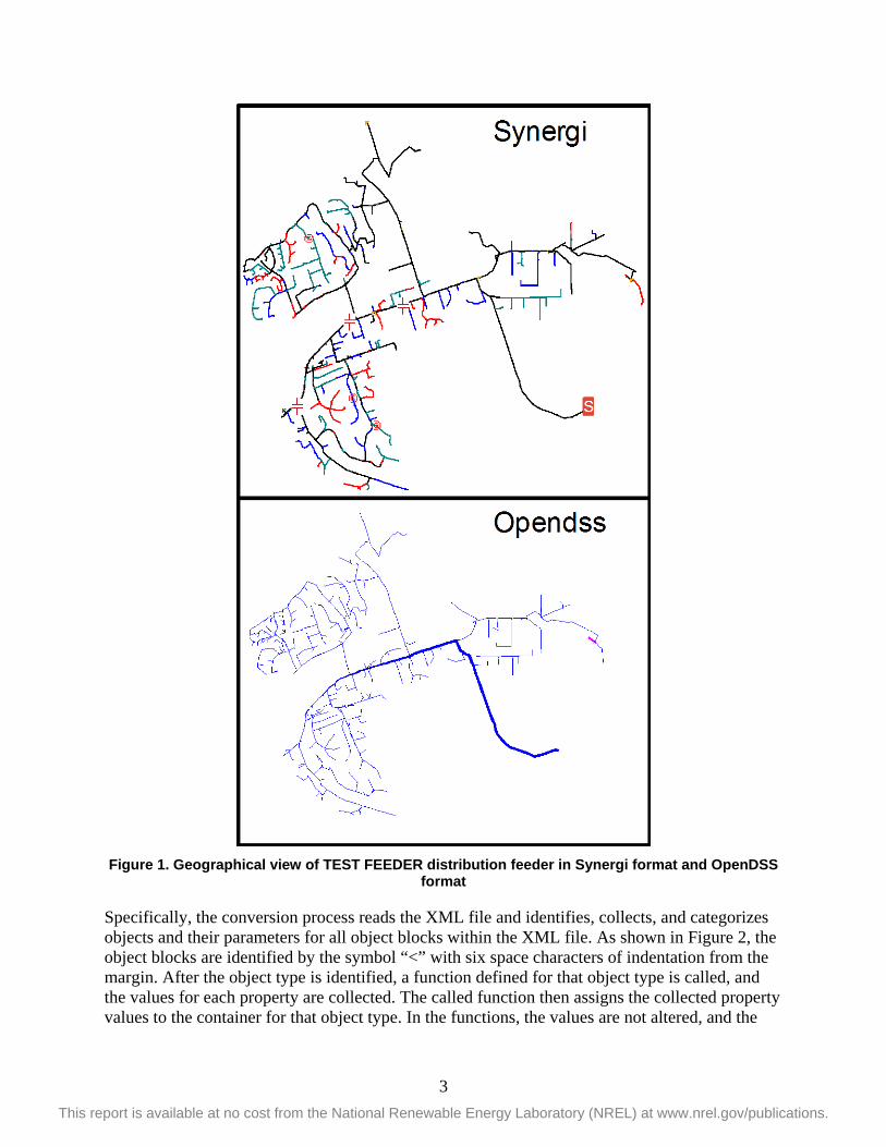
1.1.1 Model Conversion The distribution feeder selected by SDG&E, circuit TEST FEEDER, was converted from Synergi format to OpenDSS format. The geographical view of the Synergi model and OpenDSS model is shown in Figure 1.

2 This report is available at no cost from the National Renewable Energy Laboratory (NREL) at www.nrel.gov/publications.
The Synergi-to-OpenDSS conversion uses an automated Python script that takes network configuration (.xml) and line configuration (.txt) as input. To use the tool, the feeder model provided by SDG&E in Microsoft access database format was opened in Synergi and then exported in Extensible Markup Language (XML) format. Additionally, the line impedance information was extracted from Synergi using the line construction report and used as an input by the tool. The conversion tool takes the two files described (the feeder in XML format and the line construction report in text format) as inputs and creates a folder with the OpenDSS files. The user can then open the master circuit file and run it in OpenDSS.
The conversion software code is programmed in Python and is structured such that properties for each instance of a Synergi object are collected for all objects in the feeder file in XML format and then operated on via syntax or mathematical conversions to create a corresponding OpenDSS element, associated DSS file, and master circuit file.
3 This report is available at no cost from the National Renewable Energy Laboratory (NREL) at www.nrel.gov/publications.
Figure 1. Geographical view of TEST FEEDER distribution feeder in Synergi format and OpenDSS format
Specifically, the conversion process reads the XML file and identifies, collects, and categorizes objects and their parameters for all object blocks within the XML file. As shown in Figure 2, the object blocks are identified by the symbol “<” with six space characters of indentation from the margin. After the object type is identified, a function defined for that object type is called, and the values for each property are collected. The called function then assigns the collected property values to the container for that object type. In the functions, the values are not altered, and the

4 This report is available at no cost from the National Renewable Energy Laboratory (NREL) at www.nrel.gov/publications.
names of each object are kept the same as assigned in the Synergi XML file, which assists in the debugging process. The next step in the conversion process is to create objects in the OpenDSS script using the collected Synergi objects and their properties. A view of the syntax identification process is presented in Figure 2.
Figure 2. Diagram of Synergi-to-OpenDSS model conversion depicting the syntax identification process
The process of converting objects in Synergi to the equivalent objects in the OpenDSS script is not always a direct one-to-one conversion. Object types that exist in Synergi do not always exist in OpenDSS and vice versa. This is also true for the properties of objects. Switches, reclosers, and fuses are not separate objects in OpenDSS. The conversion tool creates short, low-impedance lines with switching capabilities for these components.
Finally, the converted OpenDSS script is written to a master file, and separate DSS files for each object type are created. The master file initiates a new circuit that creates a voltage source and source bus. The voltage and source impedances are specified based on data from the Synergi model. The master file also redirects to DSS component files containing scripts for the different object types separated into different categories.
1.1.2 OpenDSS Model Verification The verification of the OpenDSS model was performed based on the following metrics:
• The feeder topology for the converted model is similar to the original Synergi modelbased on visual inspection.

5 This report is available at no cost from the National Renewable Energy Laboratory (NREL) at www.nrel.gov/publications.
• The difference between the node voltages for the converted model and the originalSynergi model are less than 1%.
• The difference between the node sequence impedances for the converted model and theoriginal Synergi model needs to be as low as possible.
Figure 2 shows the feeder topology in Synergi and the converted model in OpenDSS; as shown, the line distances and coordinates are appropriately converted. The subsequent step for verification will compare the voltages obtained from OpenDSS with the Synergi voltages. Figure 3. shows the voltage profiles and voltage errors (obtained at full load) as a function of distanceand as a histogram. As shown, the voltage errors are less than 1%, and, as is typical, the voltageerrors increase toward the end of the feeder.
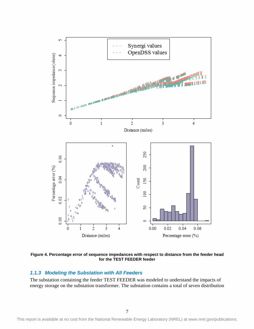
Figure 4 shows the sequence impedance profiles and errors (obtained at full load) as a function of distance and as a histogram. As shown, the sequence impedance errors are less than 0.06%, and, as is typical, the voltage errors increase toward the end of the feeder.

6 This report is available at no cost from the National Renewable Energy Laboratory (NREL) at www.nrel.gov/publications.
Figure 3. Percentage error of voltage with respect to distance from the feeder head for the TEST FEEDER feeder
7 This report is available at no cost from the National Renewable Energy Laboratory (NREL) at www.nrel.gov/publications.
Figure 4. Percentage error of sequence impedances with respect to distance from the feeder head for the TEST FEEDER feeder
1.1.3 Modeling the Substation with All Feeders The substation containing the feeder TEST FEEDER was modeled to understand the impacts of energy storage on the substation transformer. The substation contains a total of seven distribution

8 This report is available at no cost from the National Renewable Energy Laboratory (NREL) at www.nrel.gov/publications.
feeders adding up to 50 MVA catered from two 28-MVA substation transformers. The line diagram is shown in Figure 5.
Figure 5. Overview of the substation model with TEST FEEDER feeder
Among the seven distribution feeders, only one feeder (TEST FEEDER) was modeled in detail. TEST FEEDER is the distribution feeder in which the utility-scale vanadium redox flow battery (VRFB) is commissioned.
1.2 Battery Model and Details 1.2.1 Overview of Battery Characteristics A utility-scale battery energy storage system was commissioned in the distribution feeder on May 2017 at a location shown in Figure 6. The battery use cases explored are as follows: voltage regulation (droop), peak shaving, and capacity firming. NREL evaluated the impacts of the battery use cases with stacking the listed feeder support functions. Along with the battery use case evaluation, this effort identifies possible ways to monetize the benefits from the distribution feeder support.
Details of the battery use cases are as follows:
1. Voltage regulation (droop): The reactive power dispatch from the energy storage system is calculated based on the voltage (at the battery point of common coupling) using a voltage droop curve.
2. Capacity firming: In this mode, the energy storage system will smooth high-frequency power flow fluctuations at the substation to a constant or low-frequency timescale average value.
3. Peak shaving and load shifting: Load shifting is defined as displacing the power consumption of the feeder by a predefined amount for a specific time. Peak shaving is

9 This report is available at no cost from the National Renewable Energy Laboratory (NREL) at www.nrel.gov/publications.
defined as using the energy storage to regulate the peak power of the feeder within a predefined limit. Peak shaving is a special case of load shifting.
A 2-MW/4-hour battery energy storage system with redox flow battery chemistry was commissioned; the battery specifications are listed in Table 2. The battery energy storage system uses an inverter and a 480-V/12-kV transformer to connect with the grid. The specifications of the inverter are as shown in Table 3.
The active power capacity of the battery system is 2 MW, and the inverter has a capacity of 3 MVA. The inverter is oversized to accommodate increased reactive power support. Figure 7 shows the inverter’s region of operation with a circle diagram.
Table 2. Battery Specifications as Shared by Battery Manufacturer
Power rating 3 MVA
Nominal real power 2 MW
Energy capacity 8 MWh
Maximum real power 3 MW (We might never use this.)
Maximum reactive power 3 MVAR
Maximum state of charge 100%
Minimum state of charge 0%
Battery efficiency for charging Dynamic model (Section 1.2.2)
Battery efficiency for discharging Dynamic model (Section 1.2.2)
Auxiliary power services in real power Dynamic model (Section 1.2.2)

10 This report is available at no cost from the National Renewable Energy Laboratory (NREL) at www.nrel.gov/publications.
Figure 6. Topology of the distribution feeder highlighting the location of the energy storage
system
Table 3. Inverter Specifications and Control Mode
Three-phase AC voltage 480 V
Power rating 3 MVA
Maximum real power 3 MW
Maximum reactive power 3 MVAR
Frequency 60 Hz
Inverter efficiency Dynamic model (Section 1.2.2)
Real power ramp rate Infinity kW/min
Reactive power ramp rate Infinity kVAR/min

11 This report is available at no cost from the National Renewable Energy Laboratory (NREL) at www.nrel.gov/publications.
Figure 7. Inverter operation region (shaded region) shown by the circle diagram
1.3 Annual Data Analysis This section describes the methodology used to preprocess load and PV data for the time-series analysis. The distribution utility partner made a significant amount of supervisory control and data acquisition data available to NREL for this project. Table 4 summarizes the data associated with the study feeder that was used for this project.
1.3.1 Data Processing Description Table 4. Feeder Measurements
Equipment Name
Type Measurement (All Three-Phase)
Interval Range Output Interval Range
TEST FEEDER: Feeder head
Feeder breaker
P, Q, I 15-minute: 24 hours
1 minute: 24 hours
D5256 La Mesa PV irradiation
Mesonet weather station
Irradiance 5-minute: 24 hours 1 minute: 24 hours
To capture the large ramp rates associated with the PV plant variability on the feeder and to generate accurate feeder statistics, a complete 1-minute data set (i.e., 525,600 measurements per year) for 2016 was used. All missing or out-of-range supervisory control and data acquisition values were replaced with a 30-minute running average value before and after the missing data sample or group of samples.
Figure 8 presents the weather stations in the vicinity of the feeder under study. The weather station closest to the distribution under study is MIGC1, and the resolution of the PV irradiance was hourly; however, the D5256 La Mesa weather station, located approximately 6 miles north of MIGC1, had 5-minute irradiance data for the year 2016. The correlation between the E7837 weather station and the D5256 weather station is presented in Figure 9. Because the slope of the

12 This report is available at no cost from the National Renewable Energy Laboratory (NREL) at www.nrel.gov/publications.
correlation is 1.03, which is close to 1, we can confirm that the La Mesa weather station is a good replacement.
Figure 10 shows the annual load data as obtained from the utility. Four points of the year 2016 data, with a total of seven days, were missing and were filled from averages of past days. To create a “native” feeder-head load (i.e., the original load not masked by PV power production), the positive 1-minute feeder head real power was added to the negation of the real measurement from overall PV generation for each time stamp. There was a close synchronism in the time stamping of the weather station irradiance and feeder-head measurements. A sample day demonstrating the native load extraction is shown in Figure 11.
Figure 8. Locations of irradiance weather stations
MIG
E783
D525

13 This report is available at no cost from the National Renewable Energy Laboratory (NREL) at www.nrel.gov/publications.
Figure 9. La Mesa weather correlation with the Chula Vista station
Figure 10. Annual load data MW and MVAR
19 June 2016 18:45
5.672MW
22 July 2016 18:23
6.032MW 15 Aug 2016 20:18 6.25MW
26 Sep 2016 19:48 6.416MW

14 This report is available at no cost from the National Renewable Energy Laboratory (NREL) at www.nrel.gov/publications.
Figure 11. Example of creating native load
1.3.2 Results of Annual Analysis The annual data were processed as described in the previous section. Starting from gross load and PV irradiance, net load was extracted. Using the net load data and PV irradiance annual data, few analytically important days were calculated for analysis. Table 5 presents the list of days from 2016 that could be of interest for annual analysis.
Table 5. Selected Days for Analysis from 2016
Day Type Date DoY
Maximum load day September 26, 2016 270
Minimum load day March 6, 2016 65
Clear PV day April 20, 2016 111
Intermittent PV day May 21, 2016 142
Cloudy PV day January 5, 2016 5
Minimum voltage day August 15, 2016 228

15 This report is available at no cost from the National Renewable Energy Laboratory (NREL) at www.nrel.gov/publications.
Figure 12. Plot comparing DoY 111 with DoY 5. The top tile represents the substation kW and kVAR, and the bottom tile represents the sum of all PV system generation.
To aid the analysis, we developed a suite of visualization codes to capture load voltages, PV voltages, PV active/reactive power, energy storage system voltages, energy storage system active/reactive power, and voltage topology heat maps.
16 This report is available at no cost from the National Renewable Energy Laboratory (NREL) at www.nrel.gov/publications.
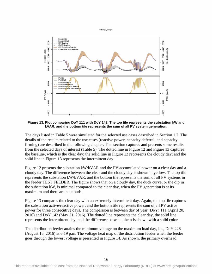
Figure 13. Plot comparing DoY 111 with DoY 142. The top tile represents the substation kW and kVAR, and the bottom tile represents the sum of all PV system generation.
The days listed in Table 5 were simulated for the selected use cases described in Section 1.2. The details of the results related to the use cases (reactive power, capacity deferral, and capacity firming) are described in the following chapter. This section captures and presents some results from the selected days of interest (Table 5). The dotted line in Figure 12 and Figure 13 captures the baseline, which is the clear day; the solid line in Figure 12 represents the cloudy day; and the solid line in Figure 13 represents the intermittent day.
Figure 12 presents the substation kW/kVAR and the PV accumulated power on a clear day and a cloudy day. The difference between the clear and the cloudy day is shown in yellow. The top tile represents the substation kW/kVAR, and the bottom tile represents the sum of all PV systems in the feeder TEST FEEDER. The figure shows that on a cloudy day, the duck curve, or the dip in the substation kW, is minimal compared to the clear day, when the PV generation is at its maximum and there are no clouds.
Figure 13 compares the clear day with an extremely intermittent day. Again, the top tile captures the substation active/reactive power, and the bottom tile represents the sum of all PV active power for three consecutive days. The comparison is between day of year (DoY) 111 (April 20, 2016) and DoY 142 (May 21, 2016). The dotted line represents the clear day, the solid line represents the intermittent day, and the difference between them is shown with a solid color.
The distribution feeder attains the minimum voltage on the maximum load day, i.e., DoY 228 (August 15, 2016) at 6:19 p.m. The voltage heat map of the distribution feeder when the feeder goes through the lowest voltage is presented in Figure 14. As shown, the primary overhead

17 This report is available at no cost from the National Renewable Energy Laboratory (NREL) at www.nrel.gov/publications.
conductor near the energy storage system location reaches 0.95 p.u. voltage and has very few laterals as well.
Figure 14. Voltage heat map of the distribution feeder at the maximum load point on August 15,
2016, at 18:19:00

18 This report is available at no cost from the National Renewable Energy Laboratory (NREL) at www.nrel.gov/publications.
2 Modeling Battery Use Cases in Distribution System Simulator
This section describes the battery model development used to simulate the battery use cases (i.e., voltage regulation, peak shaving, capacity firming) and the battery control models developed to understand the impacts of the VRFB on local grid support. The simulations were carried out using seasonal load profiles from the year 2016. The aim of this effort was to gain insight on different modes under which the battery can operate. The battery manufacturer provided the performance characteristics of the battery system that are needed for detailed modeling and cross-validation for all the use cases.
2.1 Modes of Operation The intent of this research was to develop battery control models in a distribution system analysis tool that match inverter operation in the field. The data sheet for the inverter interfacing the battery with the grid lists seven modes of operation. In this study, however, only three modes are investigated. Table 6 lists the modes of operation for the battery storage under investigation.
Table 6. Modes of Operation for Battery Storage
Higher Level Controls
1 Voltage regulation
2 Peak shaving and base loading
3 Capacity firming (smoothing)
The scope of this report is threefold. The first objective is to provide an overview for each of these modes. This also includes a brief description of the input, output, and tuning parameters. The second objective is to provide the reader with a pseudocode for the algorithms implemented in Python for each mode of operation. The third and final objective is to provide a set of simulation results that can be used to validate the design and implementation approach used in this work.
2.2 Simulation Setup The distribution feeder and the accompanying active elements (e.g., capacitors, transformers, storage) and their controllers (i.e., voltage regulator) have been implemented in OpenDSS. The high-level control modes for the battery storage listed in the previous section have been implemented using Python, a high-level open-source programming language. A direct DLL interface provided by OpenDSS has been used to facilitate communication between the OpenDSS engine and Python. The load and PV profiles saved in Comma Separated Value format (.CSV) are accessed directly by the OpenDSS engine. Figure 15 provides a graphical overview of the simulation setup.

19 This report is available at no cost from the National Renewable Energy Laboratory (NREL) at www.nrel.gov/publications.
Figure 15. Simulation setup overview
2.3 Peak Shaving and Capacity Deferral In this mode, the operator specifies the trigger values for peak shaving and base loading. The storage will discharge power into the grid if the load’s consumption (as measured) is greater than the peak shaving limit. Inversely, the energy storage system will charge if the load’s consumption at the measured point is lower than the base-loading limit.
Control Mode Overview The controller implemented for peak shaving and base loading has three modes of operation, as shown in Figure 16. Table 7 lists the modes of operation and relative parameters.
Table 7. Modes of Operation for Peak Shaving and Base Loading
Modes of Operation Relevant Parameters
1 Active power-triggered peak
shaving and base loading
𝑺𝑺𝑺𝑺𝑺𝑺: Battery state of charge (%) 𝑷𝑷𝒓𝒓𝒓𝒓𝒓𝒓: Active power measurement from reference point for peak shaving (kW) 𝑷𝑷𝒃𝒃𝒃𝒃𝒃𝒃𝒃𝒃: Battery active power output (kW) 𝑷𝑷𝑺𝑺𝑼𝑼𝑼𝑼, 𝑷𝑷𝑺𝑺𝑳𝑳𝑼𝑼: Reference set points at which peak shaving triggers (kW) 𝜟𝜟𝑷𝑷𝒃𝒃𝒃𝒃𝒃𝒃𝒃𝒃: Rate at which storage goes to idling (% of rate power)
2 Time-triggered peak shaving and base
loading
𝑷𝑷𝒃𝒃𝒃𝒃𝒃𝒃𝒃𝒃: Battery active power output (kW) 𝑻𝑻𝒉𝒉𝒓𝒓/ 𝑻𝑻𝒎𝒎𝒎𝒎𝒎𝒎: Time at which peak shaving starts 𝑻𝑻𝒄𝒄𝒄𝒄𝒓𝒓𝒉𝒉𝒓𝒓 / 𝑻𝑻𝒄𝒄𝒄𝒄𝒓𝒓𝒎𝒎𝒎𝒎𝒎𝒎: Current hour and minute 𝑷𝑷𝒅𝒅𝒄𝒄𝒉𝒉𝒅𝒅: Battery discharge set point (kW)
3 Active power- and time-triggered
All of the above
Active Power-Triggered Mode The active power-triggered mode requires two inputs: the active power threshold after which peak shaving is active and the active power measurement from the reference point for peak shaving. If the measured value exceeds the reference value and the battery state of charge (SOC) is less than 98%, the battery output is updated to cater to the difference between the measured and the reference value.
Time-Triggered Mode The time-triggered mode requires two inputs: current time and the time at which peak shaving is to be activated. If operating under this mode, the controller compares the current time with

20 This report is available at no cost from the National Renewable Energy Laboratory (NREL) at www.nrel.gov/publications.
trigger time. If the current time exceeds the trigger time, the battery starts to discharge with a constant output of 600 kW. Peak shaving continues until the battery resources have been completely depleted. Time-triggered operation does not require feedback.
Active Power-Triggered and Time-Triggered Mode Under this operational mode, peak shaving mode is set to active if both the active power-trigger and time-trigger conditions have been met. If both conditions have been met, the battery output is updated to cater to the difference between the measured and the reference value. Storage controls are iterative and converge to the steady-state solution at every time step. The error tolerance for the simulation study has been set at 0.1 kW.
Figure 16. Peak-shaving control setup
Pseudocode

21 This report is available at no cost from the National Renewable Energy Laboratory (NREL) at www.nrel.gov/publications.
Table 8. Pseudocode for Peak Shaving at Every Time Step
Simulation Results This section presents results related to peak shaving. Peak shaving was run on the peak load day for 2016, which is August 15. The algorithm for peak shaving, as described in the previous section, is implemented along with the distribution system simulator.
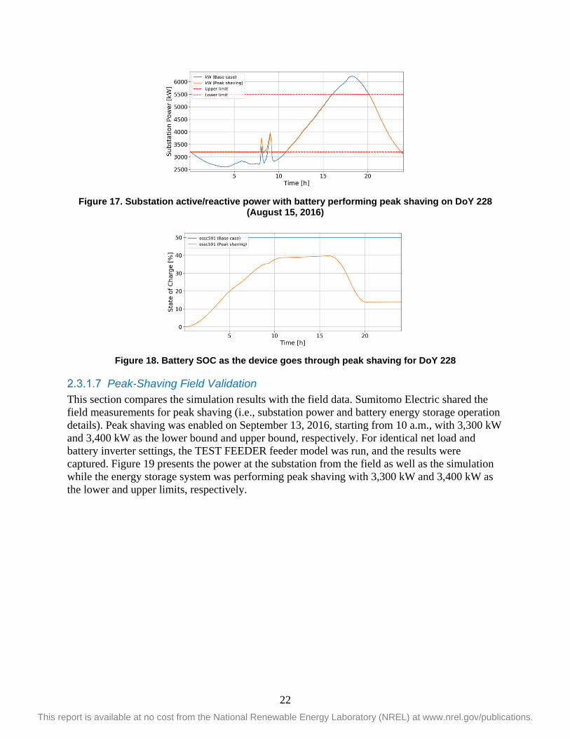
Figure 17 and Figure 18 present the active/reactive power at the substation and the battery SOC with and without peak-shaving grid support. Peak-shaving functionality charges the battery during the morning and discharges during peak hours. The charging and discharging can be enabled using either active power measurement at the substation or time of day.
Input: 𝑃𝑃𝑟𝑟𝑟𝑟𝑟𝑟[𝑡𝑡], 𝑆𝑆𝑆𝑆𝑆𝑆 [𝑡𝑡], 𝑇𝑇ℎ𝑟𝑟 ,𝑇𝑇𝑚𝑚𝑚𝑚𝑚𝑚, 𝑃𝑃𝑆𝑆𝑈𝑈𝑈𝑈, 𝑃𝑃𝑆𝑆𝐿𝐿𝑈𝑈, 𝑆𝑆𝑆𝑆𝑆𝑆𝑈𝑈𝑈𝑈 , 𝑆𝑆𝑆𝑆𝑆𝑆𝐿𝐿𝑈𝑈, 𝑀𝑀𝑀𝑀𝑀𝑀𝑀𝑀, 𝛥𝛥𝑃𝑃𝑏𝑏𝑏𝑏𝑏𝑏𝑏𝑏, 𝑃𝑃𝑑𝑑𝑑𝑑ℎ𝑔𝑔 Output: 𝑏𝑏𝑏𝑏𝑡𝑡𝑡𝑡𝑀𝑀𝑏𝑏𝑏𝑏𝑏𝑏𝑏𝑏 [𝑡𝑡 + 1] 1 if 𝑀𝑀𝑀𝑀𝑀𝑀𝑀𝑀 == 1 (Active power triggered) then 2 if (𝑃𝑃𝑟𝑟𝑟𝑟𝑟𝑟 [𝑡𝑡] > 𝑃𝑃𝑆𝑆𝑈𝑈𝑈𝑈) and 𝑆𝑆𝑆𝑆𝑆𝑆 [𝑡𝑡] < 𝑆𝑆𝑆𝑆𝑆𝑆𝑈𝑈𝑈𝑈 then 3 𝑃𝑃𝑏𝑏𝑏𝑏𝑏𝑏𝑏𝑏[𝑡𝑡 + 1] = 𝑃𝑃𝑏𝑏𝑏𝑏𝑏𝑏𝑏𝑏[𝑡𝑡] + (𝑃𝑃𝑟𝑟𝑟𝑟𝑟𝑟[𝑡𝑡] − 𝑃𝑃𝑆𝑆𝑈𝑈𝑈𝑈) 4 else if (𝑃𝑃𝑟𝑟𝑟𝑟𝑟𝑟[𝑡𝑡] < 𝑃𝑃𝑆𝑆𝐿𝐿𝑈𝑈) and 𝑆𝑆𝑆𝑆𝑆𝑆 [𝑡𝑡] > 𝑆𝑆𝑆𝑆𝑆𝑆𝐿𝐿𝑈𝑈 then 5 𝑃𝑃𝑏𝑏𝑏𝑏𝑏𝑏𝑏𝑏[𝑡𝑡 + 1] = 𝑃𝑃𝑏𝑏𝑏𝑏𝑏𝑏𝑏𝑏[𝑡𝑡] − (𝑃𝑃𝑟𝑟𝑟𝑟𝑟𝑟[𝑡𝑡] − 𝑃𝑃𝑆𝑆𝐿𝐿𝑈𝑈) 6 Else 7 if 𝑷𝑷𝒃𝒃𝒃𝒃𝒃𝒃𝒃𝒃[𝑡𝑡 + 1] < 𝐼𝐼𝑀𝑀𝐼𝐼𝐼𝐼𝐼𝐼𝐼𝐼𝐼𝐼𝑏𝑏 then 8 𝑃𝑃𝑏𝑏𝑏𝑏𝑏𝑏𝑏𝑏[𝑡𝑡 + 1] = 𝑃𝑃𝑏𝑏𝑏𝑏𝑏𝑏𝑏𝑏[t] + 𝛥𝛥𝑃𝑃𝑏𝑏𝑏𝑏𝑏𝑏𝑏𝑏 . 𝑃𝑃𝑟𝑟𝑏𝑏𝑏𝑏𝑟𝑟𝑑𝑑 9 else 10 𝑃𝑃𝑏𝑏𝑏𝑏𝑏𝑏𝑏𝑏[𝑡𝑡 + 1] = 𝑃𝑃𝑏𝑏𝑏𝑏𝑏𝑏𝑏𝑏[t] − 𝛥𝛥𝑃𝑃𝑏𝑏𝑏𝑏𝑏𝑏𝑏𝑏 . 𝑃𝑃𝑟𝑟𝑏𝑏𝑏𝑏𝑟𝑟𝑑𝑑 11 else if 𝑀𝑀𝑀𝑀𝑀𝑀𝑀𝑀 == 2 (Time triggered) then 12 if (𝑡𝑡 > 𝑇𝑇ℎ𝑟𝑟 + 𝑇𝑇𝑚𝑚𝑚𝑚𝑚𝑚 ∗ 60 ) and 𝑆𝑆𝑆𝑆𝑆𝑆 [𝑡𝑡] < 𝑆𝑆𝑆𝑆𝑆𝑆𝐼𝐼𝐼𝐼𝑆𝑆𝐼𝐼𝑡𝑡 then 13 𝑃𝑃𝑏𝑏𝑏𝑏𝑏𝑏𝑏𝑏[𝑡𝑡 + 1] = 𝑃𝑃𝑑𝑑𝑚𝑚𝑑𝑑𝑑𝑑ℎ𝑏𝑏𝑟𝑟𝑔𝑔𝑟𝑟 14 else 15 𝑃𝑃𝑏𝑏𝑏𝑏𝑏𝑏𝑏𝑏[𝑡𝑡 + 1] = 𝑃𝑃𝑏𝑏𝑏𝑏𝑏𝑏𝑏𝑏[𝑡𝑡] 16 else if 𝑀𝑀𝑀𝑀𝑀𝑀𝑀𝑀 == 3 ( Active power and Time triggered) then 17 if (𝑃𝑃𝑟𝑟𝑟𝑟𝑟𝑟 [𝑡𝑡] > 𝑃𝑃𝑀𝑀𝑑𝑑ℎ𝐼𝐼) and (𝑡𝑡 > 𝑇𝑇ℎ𝑟𝑟 + 𝑇𝑇𝑚𝑚𝑚𝑚𝑚𝑚 ∗ 60 ) and (𝑆𝑆𝑆𝑆𝑆𝑆 [𝑡𝑡] < 𝑆𝑆𝑆𝑆𝑆𝑆𝐼𝐼𝐼𝐼𝑆𝑆𝐼𝐼𝑡𝑡) then 18 𝑃𝑃𝑏𝑏𝑏𝑏𝑏𝑏𝑏𝑏[𝑡𝑡 + 1] = 𝑃𝑃𝑏𝑏𝑏𝑏𝑏𝑏𝑏𝑏[𝑡𝑡] + (𝑃𝑃𝑟𝑟𝑟𝑟𝑟𝑟[𝑡𝑡] − 𝑃𝑃𝑀𝑀𝑑𝑑ℎ𝐼𝐼) 19 Else 20 𝑃𝑃𝑏𝑏𝑏𝑏𝑏𝑏𝑏𝑏[𝑡𝑡 + 1] = 𝑃𝑃𝑏𝑏𝑏𝑏𝑏𝑏𝑏𝑏[𝑡𝑡]
22 This report is available at no cost from the National Renewable Energy Laboratory (NREL) at www.nrel.gov/publications.
Figure 17. Substation active/reactive power with battery performing peak shaving on DoY 228
(August 15, 2016)
Figure 18. Battery SOC as the device goes through peak shaving for DoY 228
Peak-Shaving Field Validation This section compares the simulation results with the field data. Sumitomo Electric shared the field measurements for peak shaving (i.e., substation power and battery energy storage operation details). Peak shaving was enabled on September 13, 2016, starting from 10 a.m., with 3,300 kW and 3,400 kW as the lower bound and upper bound, respectively. For identical net load and battery inverter settings, the TEST FEEDER feeder model was run, and the results were captured. Figure 19 presents the power at the substation from the field as well as the simulation while the energy storage system was performing peak shaving with 3,300 kW and 3,400 kW as the lower and upper limits, respectively.

23 This report is available at no cost from the National Renewable Energy Laboratory (NREL) at www.nrel.gov/publications.
Figure 19. Comparison of peak-shaving algorithm with the field data
Figure 20. Distribution of the error calculated between the field-measurement and the simulation
results
The control algorithm mimics the behavior of the battery controller very well. Figure 20 presents the histogram of the residuals between the actual field-measurement and the simulation results. The histogram shows that the residuals have a relatively low standard deviation. Other metrics used to quantify the performance of the implemented algorithm are listed in Table 9.

24 This report is available at no cost from the National Renewable Energy Laboratory (NREL) at www.nrel.gov/publications.
Table 9. Quality Metrics Calculated for the Field Measurements and Simulation Results
Metric Value Unit
Max error 341.19 kW
Error mean -3.368 kW
Error std. 21.197 kW
RMSE 21.463 kW
𝑅𝑅2 value 99.83 %
2.4 Capacity Firming (Smoothing) The basic principal behind capacity firming is improving power quality by limiting a large rate of change in active power (𝑀𝑀𝑑𝑑 𝑀𝑀𝑡𝑡⁄ ) at the measurement point. When the output power of the renewable plant changes at a rate greater than the allowed 𝑀𝑀𝑑𝑑 𝑀𝑀𝑡𝑡⁄ , storage will output power at an opposite 𝑀𝑀𝑑𝑑 𝑀𝑀𝑡𝑡⁄ to cancel out the excessive rate of change. Once the output at the point of measurement stabilizes, the output power of the energy storage system will ramp down to 0 per the operator-defined 𝑀𝑀𝑑𝑑 𝑀𝑀𝑡𝑡⁄ . The effect is that the net power at the point of common coupling will not have abrupt changes, only smooth power transitions.
Control Mode Overview` Capacity firming has two sub modes of operation, which are listed in Table 10.
Table 10. Modes of Operation for Capacity Firming
Modes of Operation Relevant Parameters
1 Without considering stabilization window
𝑷𝑷𝒓𝒓𝒓𝒓𝒓𝒓 – Active power measurement from reference point for peak shaving (kW)
𝑷𝑷𝒃𝒃𝒃𝒃𝒃𝒃𝒃𝒃 – Battery active power output (kW) 𝜟𝜟𝑷𝑷𝒍𝒍𝒎𝒎𝒎𝒎 – Ramp limit for measured point (kW/min) 𝐊𝐊 − Controller gain 𝜟𝜟𝑷𝑷𝒔𝒔𝒃𝒃𝒃𝒃𝒄𝒄𝒔𝒔 − Rate at which storage goes to idling (% of rated power)
2 With considering stabilization window
All of the above 𝑻𝑻𝒘𝒘𝒎𝒎𝒎𝒎 – Time widow during which ramp-rate stability is checked
2.4.1.1.1 Without Stability Time Horizon The first mode does not consider the stability window, and storages goes directly to idle mode (the output goes to 0 linearly using the 𝑀𝑀𝑑𝑑 𝑀𝑀𝑡𝑡⁄ limits) if 𝑀𝑀𝑑𝑑 𝑀𝑀𝑡𝑡⁄ is within prescribed limits.
2.4.1.1.2 With Stability Time Horizon The second mode of operation checks a predefined time horizon for any violations and goes to idle mode only if there are no violations within this time horizon (the internal clock waits for the event flag to clear).

25 This report is available at no cost from the National Renewable Energy Laboratory (NREL) at www.nrel.gov/publications.
Table 11. Pseudocode for Capacity Firming for Each Time Step
Capacity-Firming Field Validation This section presents simulation results pertaining to validation of the capacity firming. Figure 21 compares the simulation results with actual field data. The battery was operated in capacity-firming mode for an entire day. Because of low solar intermittence on the particular day, however, battery use is low.
Figure 21. Validation of capacity-firming algorithm using actual field data
Input: 𝑃𝑃𝑟𝑟𝑟𝑟𝑟𝑟 [𝑡𝑡], K , 𝛥𝛥𝑃𝑃𝑙𝑙𝑚𝑚𝑚𝑚 , Mode, 𝑇𝑇𝑤𝑤𝑚𝑚𝑚𝑚,𝛥𝛥𝑃𝑃𝑑𝑑𝑏𝑏𝑏𝑏𝑑𝑑𝑠𝑠 Output: batterykW [𝑡𝑡 + 1] 1 𝛥𝛥𝑃𝑃𝑟𝑟𝑟𝑟𝑟𝑟[𝑡𝑡] = 𝑃𝑃𝑟𝑟𝑟𝑟𝑟𝑟 [𝑡𝑡] – 𝑃𝑃𝑟𝑟𝑟𝑟𝑟𝑟 [𝑡𝑡 − 1] 2 if 𝛥𝛥𝑃𝑃𝑟𝑟𝑟𝑟𝑟𝑟[𝑡𝑡] > 𝛥𝛥𝑃𝑃𝑙𝑙𝑚𝑚𝑚𝑚 or 𝛥𝛥𝑃𝑃𝑟𝑟𝑟𝑟𝑟𝑟[𝑡𝑡] < – 𝛥𝛥𝑃𝑃𝑙𝑙𝑚𝑚𝑚𝑚 then 3 ∆𝑃𝑃𝑏𝑏𝑏𝑏𝑏𝑏𝑏𝑏 [𝑡𝑡] = K.𝛥𝛥𝑃𝑃𝑟𝑟𝑟𝑟𝑟𝑟[𝑡𝑡]. [1 − 𝛥𝛥𝑃𝑃𝑙𝑙𝑚𝑚𝑚𝑚 / |𝛥𝛥𝑃𝑃𝑟𝑟𝑟𝑟𝑟𝑟[𝑡𝑡]| ] 4 EventFlag = 𝑡𝑡 5 else 6 if Mode == 1 and Battey_Idle == False then 7 ∆𝑃𝑃𝑏𝑏𝑏𝑏𝑏𝑏𝑏𝑏[𝑡𝑡] = 𝑃𝑃𝑟𝑟𝑟𝑟𝑟𝑟[𝑡𝑡]/|𝑃𝑃𝑟𝑟𝑟𝑟𝑟𝑟[𝑡𝑡]| . –𝛥𝛥𝑃𝑃𝑑𝑑𝑏𝑏𝑏𝑏𝑑𝑑𝑠𝑠 . 𝑃𝑃𝑟𝑟𝑏𝑏𝑏𝑏𝑟𝑟𝑑𝑑 8 else if Mode == 2 and Battey_Idle == False and 𝑡𝑡 − EventFlag > 𝑇𝑇𝑤𝑤𝑚𝑚𝑚𝑚 then 9 ∆𝑃𝑃𝑏𝑏𝑏𝑏𝑏𝑏𝑏𝑏[𝑡𝑡] = 𝑃𝑃𝑟𝑟𝑟𝑟𝑟𝑟[𝑡𝑡]/|𝑃𝑃𝑟𝑟𝑟𝑟𝑟𝑟[𝑡𝑡]| . – StepBackRate. 𝑃𝑃𝑟𝑟𝑏𝑏𝑏𝑏𝑟𝑟𝑑𝑑 10 Else 11 ∆𝑃𝑃𝑏𝑏𝑏𝑏𝑏𝑏𝑏𝑏[𝑡𝑡] = 0 12 𝑃𝑃𝑏𝑏𝑏𝑏𝑏𝑏𝑏𝑏[𝑡𝑡 + 1] = 𝑃𝑃𝑏𝑏𝑏𝑏𝑏𝑏𝑏𝑏[𝑡𝑡] + ∆𝑃𝑃𝑏𝑏𝑏𝑏𝑏𝑏𝑏𝑏[𝑡𝑡]
26 This report is available at no cost from the National Renewable Energy Laboratory (NREL) at www.nrel.gov/publications.
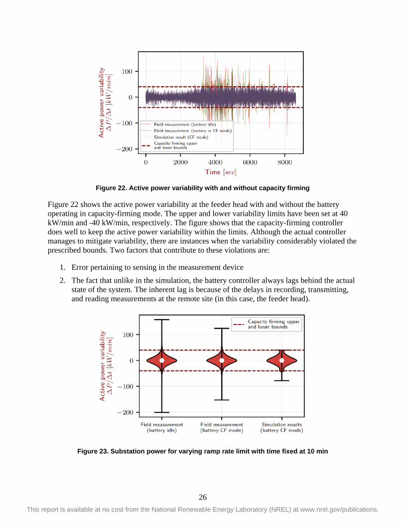
Figure 22. Active power variability with and without capacity firming
Figure 22 shows the active power variability at the feeder head with and without the battery operating in capacity-firming mode. The upper and lower variability limits have been set at 40 kW/min and -40 kW/min, respectively. The figure shows that the capacity-firming controller does well to keep the active power variability within the limits. Although the actual controller manages to mitigate variability, there are instances when the variability considerably violated the prescribed bounds. Two factors that contribute to these violations are:
1. Error pertaining to sensing in the measurement device
2. The fact that unlike in the simulation, the battery controller always lags behind the actual state of the system. The inherent lag is because of the delays in recording, transmitting, and reading measurements at the remote site (in this case, the feeder head).
Figure 23. Substation power for varying ramp rate limit with time fixed at 10 min
27 This report is available at no cost from the National Renewable Energy Laboratory (NREL) at www.nrel.gov/publications.
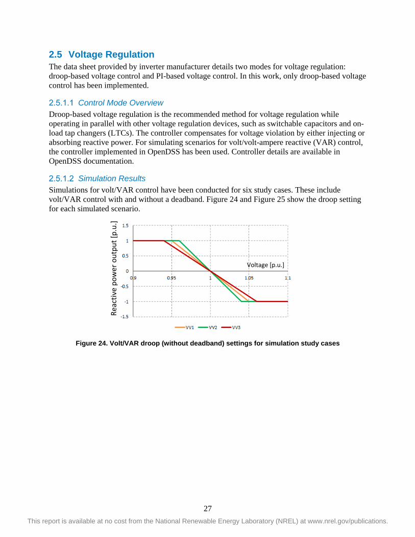
2.5 Voltage Regulation The data sheet provided by inverter manufacturer details two modes for voltage regulation: droop-based voltage control and PI-based voltage control. In this work, only droop-based voltage control has been implemented.
Control Mode Overview Droop-based voltage regulation is the recommended method for voltage regulation while operating in parallel with other voltage regulation devices, such as switchable capacitors and on-load tap changers (LTCs). The controller compensates for voltage violation by either injecting or absorbing reactive power. For simulating scenarios for volt/volt-ampere reactive (VAR) control, the controller implemented in OpenDSS has been used. Controller details are available in OpenDSS documentation.
Simulation Results Simulations for volt/VAR control have been conducted for six study cases. These include volt/VAR control with and without a deadband. Figure 24 and Figure 25 show the droop setting for each simulated scenario.
Figure 24. Volt/VAR droop (without deadband) settings for simulation study cases
Voltage [p.u.]
Reac
tive
pow
er o
utpu
t [p.
u.]

28 This report is available at no cost from the National Renewable Energy Laboratory (NREL) at www.nrel.gov/publications.
Figure 25. Volt/VAR droop (with deadband) settings for simulation study cases
Figure 26. Storage reactive power output for voltage support mode
The simulation study has been run for a day with high peak load and renewable generation corresponding to DoY 228. Figure 26 captures the reactive power support from the energy storage system (per phase) for all volt/VAR curves (VV1 to VV6). Volt/VAR curves with 3% deadband do not enable the energy storage system for reactive power support. As shown in Figure 26, for curves VV4, VV5, and VV6, reactive power support is insignificant.
The results in Figure 27 show that running the battery in volt/VAR mode can potentially improve the voltage profile by providing reactive power support, particularly for volt/VAR curves without any deadband. The maximum change in storage reactive power output is approximately 20% of overall capacity, or 600 kVAR (sum of three phases).
Reac
tive
pow
er o
utpu
t [p.
u.]
Voltage [p.u.]

29 This report is available at no cost from the National Renewable Energy Laboratory (NREL) at www.nrel.gov/publications.
Figure 27. Voltage profile for voltage-support mode

30 This report is available at no cost from the National Renewable Energy Laboratory (NREL) at www.nrel.gov/publications.
3 Energy Storage Value Streams from Distribution Support
3.1 Introduction and Background This section identifies methods to evaluate the monetary value derived from the VRFB energy storage system by providing distribution support. The purpose of this task is to monetize the benefits from distribution support, such as voltage regulation, capacity firming, and peak shaving. For the optimization, each benefit needs to be converted into a monetary value that the model can chose between. This section performs a detailed literature review and develops effective ways to evaluate cost-benefits for feeder support functions.
This work also involves formulating and solving the optimization problem using NREL’s Renewable Energy Optimization (REopt) model.1 The optimization solver will be used to generate operation profiles that maximize benefits from the energy storage system. The methods to monetize the feeder support functions derived from the prior task will be implemented to generate optimal operation profiles.
The description in the chapter will focus on gaining real-world experience and data from distribution-connected battery energy storage system operation and evaluating the value provided by this system.
3.2 Value Streams for Distribution Grid Support Monetization This section describes the potential value streams that could be realized through appropriate dispatch of the VRFB system. The VRFB battery is connected as a distribution system asset and considered to be under full utility ownership and control. Distribution assets are managed by the SDG&E Distribution Control Center.
First, the three main battery applications are described in brief, and the potential value streams are outlined. Then, a description of the TEST FEEDER feeder characteristics is presented, and the modeling approaches for monetizing specific value streams are identified. Finally, the simulation framework for the VRFB value stacking using an optimal dispatch model is described.
3.2.1 Applications Chosen for Distribution Grid Support The battery applications in this project focus on providing distribution system support services as follows:
• Peak shaving: Energy storage charges during low-load periods and discharges during high-load periods to reduce the peak demand on the feeder during the highest loading condition.
• Capacity firming: The objective of capacity firming is to use storage to smooth the output of intermittent renewable energy generation. Storage is able to react quickly to
1 https://reopt.nrel.gov/

31 This report is available at no cost from the National Renewable Energy Laboratory (NREL) at www.nrel.gov/publications.
compensate for rapid fluctuations in output, resulting in reduced ramping and a more consistent, less variable load on the system.
• Voltage support: Energy storage can also provide voltage support to maintain feeder voltages within acceptable bounds, typically ±5% of nominal. For sensitive electric appliances and electronics, it is important that voltage is supplied within these limits. Utilities typically install capacitor banks or voltage regulators to boost the voltage at the end of a line. With power electronics capable of injecting and absorbing both real and reactive power at different rates, energy storage is now able to provide the same services.
The value streams listed in the sections below have been explored to identify monetary benefits from a battery. The value streams identified by NREL are described in the following sections.
Value Streams from Peak Shaving An energy storage system capable of reducing peak system loading is assumed to be able to offset all or part of an investment toward substation or distribution circuit upgrades. To quantify the value of an upgrade deferral, the following information is required:
• System loading level at which an upgrade is required
• Cost of upgrades
• Forecasted load growth on the network (to establish when limits will be met/exceeded with and without the storage system).
To capture the value from providing a distribution upgrade deferral, the battery storage system must be able to continuously keep the overall network demand less than a predetermined level.
Value Streams from Capacity Firming 3.2.1.2.1 Substation Capacity Firming Capacity firming can reduce the number of LTC operations required at the substation level, resulting in a reduction of operation and maintenance (O&M) costs.
3.2.1.2.2 Renewables Capacity Firming Storage coupled with PV can firm highly variable generation output. If a capacity market exists, PV production alone might not coincide with capacity needs (e.g., when the capacity is called for and/or tested to establish total available capacity). A battery system can be used to firm PV output during critical hours, increasing the total capacity payment that a stand-alone PV system can achieve.
Value Streams from Voltage Support The uncertainty and variability introduced by distributed PV increases the need for flexible reactive power support. Additional capacitor banks are required to regulate system voltages. Currently, utilities maintain voltages within specified limits using tap-changing regulators at the distribution substation and by switching capacitors to follow changes in load. This is especially important on long, radial feeders where a large load such as an arc welder or a residential PV system might cause unacceptable voltage excursions for neighboring customers. An energy storage system can effectively dampen these voltage fluctuations by discharging small amounts of active power.

32 This report is available at no cost from the National Renewable Energy Laboratory (NREL) at www.nrel.gov/publications.
There is currently no financial compensation for reactive power services in distribution networks. One way to account for the increasing demand for flexible reactive power support in distribution systems is to replicate the lost opportunity cost model currently used with spinning generation at the transmission level.
Value Streams from Energy Arbitrage Energy storage is charged during off-peak hours and discharged during peak hours to take advantage of the price difference of electricity across time periods. The revenue obtained is the price differential between buying and selling electrical energy minus the cost of losses during the full charge/discharge cycle.
Although market participation is not the focus of the current phase of the project, the value of energy arbitrage is modeled to fully capture the economic impacts of battery operation to provide other distribution system services.
Stacking Value Streams for Multiuse A storage system used for upgrade deferral can simultaneously provide voltage support and capacity firming. Value streams might be stacked, with multiple services provided through a single asset. The added value provided by this flexibility could be quantified and assigned to the battery system as an additional benefit.
3.2.2 Distribution Feeder and Substation Conditions The TEST FEEDER feeder that the VRFB system are located on is one of seven feeders that connect to the distribution substation. This substation has two 28-MVA LTC transformer banks built out and two free spots for potential banks in the future. The existing LTC banks operate in parallel and have the ability to support 100–110% loading for 30–60 minutes. OpenDSS analyses show that under current loading conditions, voltages along the feeder are all within the operating limit from 0.95–1.05 p.u. Capacitor banks are present on the feeder, but no regulators are installed. Load growth on the feeder is estimated to be 3% per year.
A combination of low feeder load and high PV penetration causes the feeder head to experience power export: up to -500 kW was measured during the commissioning phase; however, there is no active curtailment of PV systems at the distribution level. Although system operators can curtail renewable energy to maintain generation on baseload units at the transmission level, this does not impact the feeder directly, and the VRFB system cannot reduce that curtailment.

33 This report is available at no cost from the National Renewable Energy Laboratory (NREL) at www.nrel.gov/publications.
Figure 28. OpenDSS diagram of feeder TEST FEEDER showing the capacity-constrained line
A portion of the TEST FEEDER feeder between the VRFB and the primary connecting to the substation is capacity constrained (Figure 28). This 1.5-mile #6 overhead cable has a maximum rating of 2.25 MVA, and it directly impacts the maximum charging capacity of the VRFB system. Because the VRFB system is installed downstream of the capacity-constrained line, the total load from that point of the feeder and below along with battery charging power cannot exceed 2.25 MVA. For example, if the load below the capacity-constrained line is measured at 500 kW, then the battery must charge at or less than 1.75 MW (less than its 2-MW total inverter rating).
This constraint is considered in the modeling approach. Loads less than the capacity-constrained line are continuously monitored to ensure that battery charging in optimized dispatches never exceeds the line limits unless a line upgrade cost is paid. Optimizations are solved with the option to respect charging constraints based on feeder load at each time step or pay the upgrade cost and avoid all charging limitations.
The line upgrade cost was estimated using past projects from rate case testimonies (Jenkins 2014). The cost of aluminum cables was averaged among all relevant projects found, and it determined to be approximately $84.53/ft. This unit cost includes material, labor, direct charges, contract costs, and contingency, making the total cost of upgrading the 1.5-mile line approximately $670,000. This value is likely to be an underestimation because potential site-specific considerations and other component costs (e.g., poles, cross-arms) are not considered; however, this cost penalty was sufficient to disincentivize line upgrades in the scenarios considered in this analysis.
Capacity Constrained

34 This report is available at no cost from the National Renewable Energy Laboratory (NREL) at www.nrel.gov/publications.
3.3 Framework for Value Stream Modeling and Comparison To quantify the monetary value provided by the VRFB storage system through the value streams listed in Section 3.2.1 two scenarios—with and without storage—are compared:
• Benchmark scenario: A multiyear simulation is performed assuming no storage system is installed to determine:
o LTC transformer upgrade required to meet demand growth
o Total cost of electricity purchased on the locational marginal price (LMP) market
o Additional capacitor investments required for reactive power and voltage support to ensure system reliability
o Baseline levels of LTC and capacitor switching to maintain power quality.
• Utility-storage scenario: A multiyear simulation is performed accounting for the VRFB installation, and new distribution system investment and operation costs are determined. It is assumed that the battery is located on the utility side of the meter, with the utility having full control of its operation. This simulation will leverage data from OpenDSS runs to accurately capture how the VRFB system can be used in different grid support modes. Further, the REopt model will be used to optimally trade-off between value streams and to determine how the VRFB system should be operated to achieve its maximum revenue potential as it provides distribution grid support services.
The value of the VRFB system is quantified as the difference between these two scenarios. Details about how different value streams are monetized are listed in Figure 32 along with an explanation of how deferral value is calculated in this analysis.
3.3.1 Calculating the Value of Distribution Upgrade Deferral This section outlines the set of value streams that are assessed in this analysis. This set of value streams is determined by checking whether each potential value stream in Section 2.2.4.2 applies to the distribution feeder substation network. Because a primary way the VRFB system captures value by providing distribution system support services is through the deferral of existing equipment upgrades or new asset installations, an example calculation of how deferral value is quantified is provided first.
To quantify the monetary value of an asset upgrade or installation deferral, the total value of the deferral is first determined and then converted to a $/kW amount for each kW of battery capacity allocated toward providing a specific service. An example calculation is shown in Figure 29.
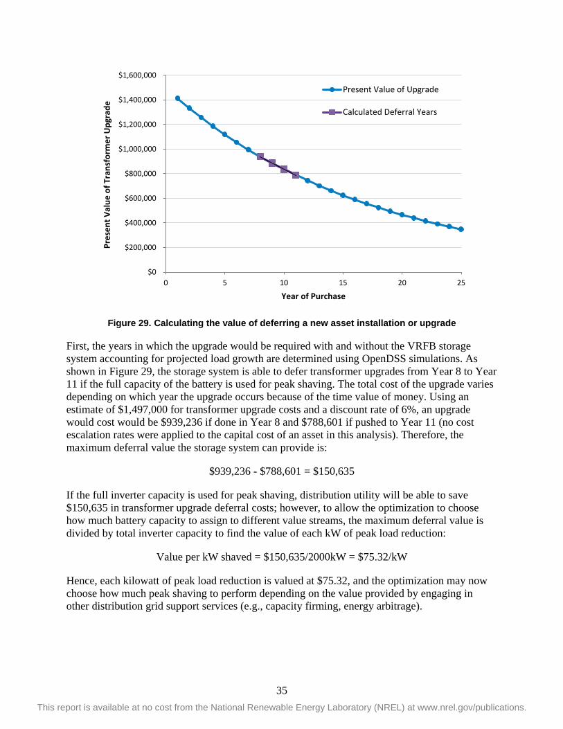
35 This report is available at no cost from the National Renewable Energy Laboratory (NREL) at www.nrel.gov/publications.
Figure 29. Calculating the value of deferring a new asset installation or upgrade
First, the years in which the upgrade would be required with and without the VRFB storage system accounting for projected load growth are determined using OpenDSS simulations. As shown in Figure 29, the storage system is able to defer transformer upgrades from Year 8 to Year 11 if the full capacity of the battery is used for peak shaving. The total cost of the upgrade varies depending on which year the upgrade occurs because of the time value of money. Using an estimate of $1,497,000 for transformer upgrade costs and a discount rate of 6%, an upgrade would cost would be $939,236 if done in Year 8 and $788,601 if pushed to Year 11 (no cost escalation rates were applied to the capital cost of an asset in this analysis). Therefore, the maximum deferral value the storage system can provide is:
$939,236 - $788,601 = $150,635
If the full inverter capacity is used for peak shaving, distribution utility will be able to save $150,635 in transformer upgrade deferral costs; however, to allow the optimization to choose how much battery capacity to assign to different value streams, the maximum deferral value is divided by total inverter capacity to find the value of each kW of peak load reduction:
Value per kW shaved = $150,635/2000kW = $75.32/kW
Hence, each kilowatt of peak load reduction is valued at $75.32, and the optimization may now choose how much peak shaving to perform depending on the value provided by engaging in other distribution grid support services (e.g., capacity firming, energy arbitrage).
$0
$200,000
$400,000
$600,000
$800,000
$1,000,000
$1,200,000
$1,400,000
$1,600,000
0 5 10 15 20 25
Pres
ent V
alue
of T
rans
form
er U
pgra
de
Year of Purchase
Present Value of Upgrade
Calculated Deferral Years

36 This report is available at no cost from the National Renewable Energy Laboratory (NREL) at www.nrel.gov/publications.
3.3.2 Framework for Peak Shaving Distribution upgrade deferral is achieved through peak shaving. The VRFB system is able to decrease peak loading at the test distribution substation, thus deferring when a transformer upgrade must occur.
To calculate the value of this deferral, the year in which the distribution substation will require a transformer upgrade with and without the VRFB system is determined. The maximum deferral value the battery can provide is the difference in present value of the cost of transformer upgrade in the two out-years. This is translated into a $/kW value, where each kW of peak reduced captures a portion of the total deferral value.
Transformer upgrade costs were estimated using past projects costs from the distribution utility rate case testimony documents (Jenkins 2014). SDG&E identified the Salt Creek and Mira Sorrento substation projects as the sites most comparable to the distribution substation. Therefore, an average of the relevant component costs from both of these projects were used to estimate the transformer upgrade cost at substation. Table 12 shows the breakdown of how total transformer upgrade costs were derived.
Table 12. Distribution Substation Transformer Upgrade Costs
Component Cost
Transformer bank (30 MW) $1,164,000
Circuit breaker $91,000
Disconnect switch $64,000
Control panel $178,000
Total $1,497,000
3.3.3 Framework for Capacity Firming Substation capacity firming allows LTC operations to be reduced. If significant LTC operation reduction is possible, the associated O&M reduction along with the battery capacity necessary to achieve the required level of substation capacity firming are added to the optimization model as a potential revenue stream. The impact of the VRFB system on LTC operations is evaluated by operating the energy storage system in capacity-firming mode and evaluating the corresponding impact at the substation. Because of the lack of a capacity market in the California Independent System Operator (CAISO) territory, renewables capacity firming is not evaluated in this analysis.
3.3.4 Framework for Voltage Support The value of voltage support is quantified through the deferral of new capacitor bank installations along the feeder where the VRFB system is located and through reductions in O&M costs for existing capacitor and LTC banks:
• New capacitor bank deferral: Similar to the transformer upgrade deferral calculations, the value of capacitor bank deferral is calculated by establishing when an installation or upgrade is required with and without the VRFB system and then taking the difference in the present value of the installation/upgrade cost in the out-years.

37 This report is available at no cost from the National Renewable Energy Laboratory (NREL) at www.nrel.gov/publications.
• Reduced O&M for capacitor and LTC banks: Changes in capacitor and LTC use because of the VRFB system are assessed in OpenDSS, and O&M savings as a result of reduced switching are quantified.
These values streams can be stacked directly without impacting other grid support functions in most circumstances because the inverters of the VRFB can supply 1 MVAR of reactive power capacity without impacting the real power output of the system. Consequently, these value streams are not modeled within the optimization because they do not compete with the other value streams for battery capacity. OpenDSS is used to confirm that 1 MVAR is sufficient to perform the required voltage support services.
New capacitor bank costs were estimated using past project costs found in the SDG&E rate case testimonies (Jenkins 2014). Six separate costs were found for the 1,200-kVAR pad-mounted capacitors from five different projects (Table 13). Costs were given per capacitor and cover material, labor, direct charges, contract costs, and contingency. A distinction was made for whether the capacitor was installed in a new area or through an intercept conduit. Without additional information about how new capacitors might be installed on the TEST FEEDER feeder, the new capacitor bank cost was assumed to be the average of all previously identified costs: $56,054.
Table 13. Costs for 1,200-kVAR Pad-Mounted Capacitors in Past SDG&E Projects
Project Intercept Conduit New Area
C928, POM: new 12-kV circuit $57,200 -
C1288, MSH: new 12-kV circuit - $56,100
C1090, JM: new 12-kV circuit $101,200 -
C1120, BQ: new 12-kV circuit $57,200 $35,750
GH new 12-kV circuit - $28,875
Average $56,054
3.3.5 Framework for Energy Arbitrage It is assumed that the utility purchases the energy required to meet the network load on the LMP market (through some combination of day-ahead and real-time markets). With the VRFB system, the utility is able to charge the battery during low-price hours and discharge during high-price hours to take advantage of the price differential. The battery dispatch can be optimized to reduce the cost to the utility of purchasing the electricity needed to serve its customers.
The value of energy arbitrage is modeled with 2016 day-ahead LMP data from the nearest LMP node to the distribution substation (TELECYN_1_014). The cost of energy at each hour is used an input to the optimization to inform the trade-offs of using battery capacity to capture different value streams.

38 This report is available at no cost from the National Renewable Energy Laboratory (NREL) at www.nrel.gov/publications.
Table 14. Statistics for the 2016 LMP Signal Used in This Analysis
Minimum ($/MW)
Maximum ($/MW)
Average ($/MW)
Median ($/MW)
Standard Deviation ($/MW)
-$27.70 $180.60 $29.60 $27.70 $13.80
Table 14 outlines basic statistics around the LMP signal, and Figure 31 show how prices vary throughout the day and during the course of the year. The average 2016 LMP value at the TELECYN_1_014 node is approximately $30/MW with a standard deviation of $13.80/MW. Prices are typically highest in the evening between 5–8 p.m.; and lowest throughout the night, from 12–4 a.m., or during midday, from 8 a.m.–4 p.m. A less distinct morning peak between 5–8 a.m. is seen in some months (e.g., late fall/winter). Prices tend to trend upward slightly in the summer months (June–September), with higher daytime prices seen.
Figure 30. LMP values throughout 2016
-50
0
50
100
150
200
LMP
Sign
al [$
/MW
]
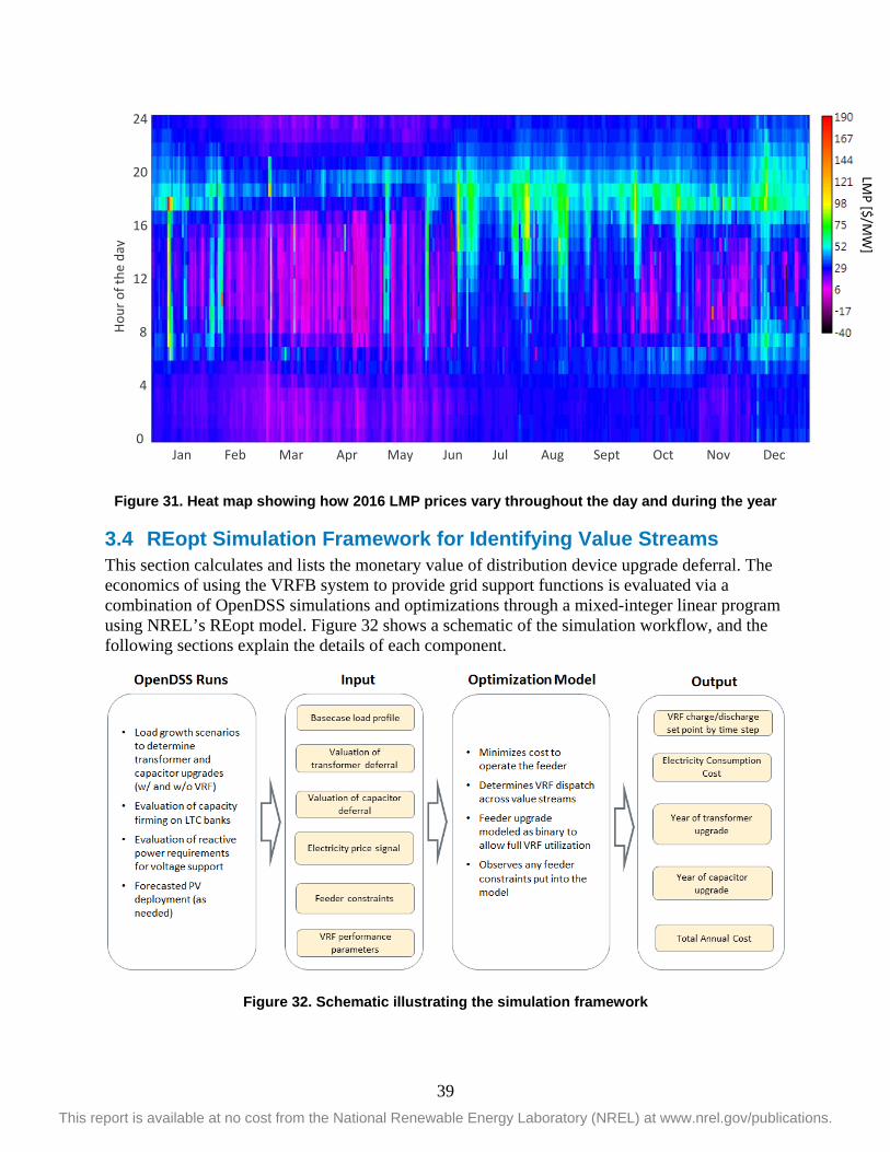
39 This report is available at no cost from the National Renewable Energy Laboratory (NREL) at www.nrel.gov/publications.
Figure 31. Heat map showing how 2016 LMP prices vary throughout the day and during the year
3.4 REopt Simulation Framework for Identifying Value Streams This section calculates and lists the monetary value of distribution device upgrade deferral. The economics of using the VRFB system to provide grid support functions is evaluated via a combination of OpenDSS simulations and optimizations through a mixed-integer linear program using NREL’s REopt model. Figure 32 shows a schematic of the simulation workflow, and the following sections explain the details of each component.
Figure 32. Schematic illustrating the simulation framework
Jan Feb Mar Apr May Jun Jul Aug Sept Oct Nov Dec
24 20 16 12 8 4 0
Hour
of t
he d
ay
LMP [$/M
W]
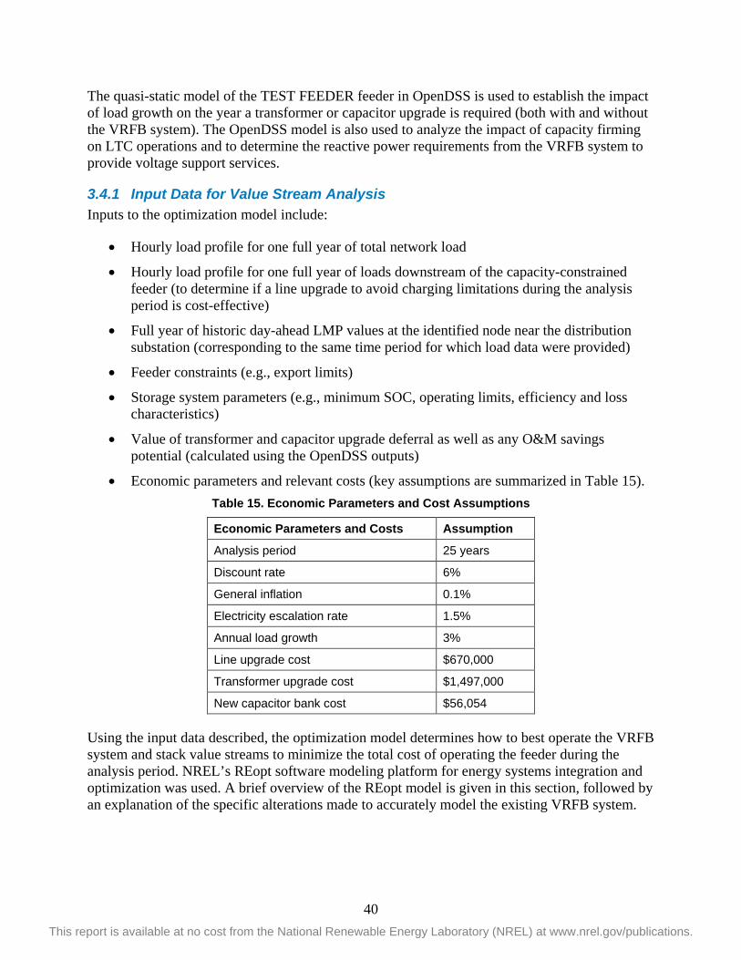
40 This report is available at no cost from the National Renewable Energy Laboratory (NREL) at www.nrel.gov/publications.
The quasi-static model of the TEST FEEDER feeder in OpenDSS is used to establish the impact of load growth on the year a transformer or capacitor upgrade is required (both with and without the VRFB system). The OpenDSS model is also used to analyze the impact of capacity firming on LTC operations and to determine the reactive power requirements from the VRFB system to provide voltage support services.
3.4.1 Input Data for Value Stream Analysis Inputs to the optimization model include:
• Hourly load profile for one full year of total network load
• Hourly load profile for one full year of loads downstream of the capacity-constrained feeder (to determine if a line upgrade to avoid charging limitations during the analysis period is cost-effective)
• Full year of historic day-ahead LMP values at the identified node near the distribution substation (corresponding to the same time period for which load data were provided)
• Feeder constraints (e.g., export limits)
• Storage system parameters (e.g., minimum SOC, operating limits, efficiency and loss characteristics)
• Value of transformer and capacitor upgrade deferral as well as any O&M savings potential (calculated using the OpenDSS outputs)
• Economic parameters and relevant costs (key assumptions are summarized in Table 15). Table 15. Economic Parameters and Cost Assumptions
Economic Parameters and Costs Assumption
Analysis period 25 years
Discount rate 6%
General inflation 0.1%
Electricity escalation rate 1.5%
Annual load growth 3%
Line upgrade cost $670,000
Transformer upgrade cost $1,497,000
New capacitor bank cost $56,054
Using the input data described, the optimization model determines how to best operate the VRFB system and stack value streams to minimize the total cost of operating the feeder during the analysis period. NREL’s REopt software modeling platform for energy systems integration and optimization was used. A brief overview of the REopt model is given in this section, followed by an explanation of the specific alterations made to accurately model the existing VRFB system.

41 This report is available at no cost from the National Renewable Energy Laboratory (NREL) at www.nrel.gov/publications.
3.4.2 REopt Overview The REopt model is based on a mixed-integer linear program that seeks to minimize the life-cycle cost of energy at a site during the analysis period, subject to a variety of constraints. The life-cycle cost of energy considers:
• All of the costs associated with providing energy to the site, including the cost of purchasing energy from the utility grid or wholesale electricity market
• The capital cost of building new technologies
• All O&M costs
• Income from utility or state incentive programs
• Any tax benefits.
The model performs an hourly simulation of the energy system, solving an energy balance at every time step where loads must be met by some combination of renewable and conventional generation, purchased energy from the utility grid or wholesale electricity market, discharges from energy storage, or dispatchable loads. This energy balance is solved for the first year and then assumed to repeat for each of the ensuing years in the analysis period. The output of the REopt model is a set of cost-optimal sizes for each technology in the candidate pool and the net present value that is achieved if the technologies in the solution are implemented. The optimal dispatch strategy for each technology required to achieve the net present value is also provided.
The technology sizing and selection components of REopt were not used in this study. Building additional renewable energy generation to potentially reduce feeder operation costs was not considered, and sizing for the storage system was based on specifications of the existing VRFB. The analysis focused on modeling the existing battery as accurately as possible to determine an optimal dispatch strategy that minimizes total life-cycle costs through stacking all monetizable value streams.
For mathematical formulations and additional details of the REopt model, see Cutler et al. (2017).
3.4.3 VRFB Loss Modeling in REopt To accurately capture VRFB performance characteristics, total system losses are modeled within REopt based on field data from the existing VRFB system. Total system losses are separated into three main sources of loss: power conditioning system (PCS) losses, storage losses, and the auxiliary power consumption of the electrolyte pump. It is assumed that the battery has no other loss components. Because REopt is a mixed-integer linear program, losses were derived as linear functions of explanatory variables.
Within the optimization, PCS and storage losses are combined and modeled together as functions of active power. Two separate equations were derived: one for losses during battery charging and one for losses during battery discharging. Figure 33 shows the linear fits of the combined PCS and storage losses field data points as a function of the charging and discharging power. The R-squared values for each show that a linear fit aligns closely with observed measurements.

42 This report is available at no cost from the National Renewable Energy Laboratory (NREL) at www.nrel.gov/publications.
Figure 33. Linearized PCS and storage losses as a function of charging/discharging power
It is assumed that the VRFB system serves both the PCS and storage losses. These losses decrease the available charge in the battery and impact its operation in future time steps.
The third loss component is the power consumption of the auxiliary pumps. This was determined to be a function of the active power as well as the battery SOC. The top two plots in Figure 33 show the field data of auxiliary power consumption across the full SOC range for separate charging and discharging rates. To linearize this complex behavior, auxiliary power consumption modeling is split into five regimes:
• Charging to less than 60% SOC: Because the battery is at a low SOC, relatively little pumping power is required to raise the SOC. Auxiliary power consumption is modeled as a constant 18.4 kW in this regime.
• Charging to more than 60% SOC: Pumping power requirements increase the more the battery is trying to charge close to full SOC. Auxiliary power consumption data are first averaged among different charging rates at each SOC level, and a linear fit is done using the new data points (bottom left plot in Figure 33). Pump consumption is modeled as a linear function of SOC for battery operation in this regime.
• Discharging to less than 60% SOC: Pumping power requirements also increase the more the battery is trying to discharge when it is nearly drained. Auxiliary power consumption data are first averaged among different discharging rates at each SOC level, and a linear fit is done using the new data points (bottom right plot in Figure 33). Pump consumption is modeled as another linear function of SOC for battery operation in this regime.
• Discharging to more than 60% SOC: Because the battery is at a high SOC, relatively little pumping power is required to meet the requested discharge rate. Auxiliary power consumption data are averaged among the different discharge powers to arrive at a constant 12.9-kW pump consumption rate for any operation within this regime.
y = -0.1163xR² = 0.9663
y = 0.1488xR² = 0.9178
0
50
100
150
200
250
-1500 -1000 -500 0 500 1000 1500
Loss
es [k
W]
Charging/discharging power [kW]

43 This report is available at no cost from the National Renewable Energy Laboratory (NREL) at www.nrel.gov/publications.
• Idling: Two scenarios are compared for auxiliary power consumption when the battery is neither charging nor discharging, but based on input from battery manufacturer, Scenario 2 is assumed for all results presented in Chapter 3:
o Scenario 1: A constant 18.4-kW pump consumption is modeled to maintain electrolyte circulation when the battery is idle.
o Scenario 2: Pumps shut off when the battery is idle, consuming no energy. It is assumed that the system can restart in a negligible amount of time so that the ability of the battery to capture any of the modeled value streams is unaffected. It is also assumed that frequent restarts do not increase degradation or other equipment O&M costs enough to introduce an additional cost to the analysis.
Figure 34. Auxiliary power consumption during charging and discharging as a function of SOC
Pump losses are modeled as external to the battery. The auxiliary power consumption is costed at LMP and factored into revenue calculations, but it does not directly subtract from the battery SOC. The VRFB system is allowed to supply its own auxiliary load if it is economical to do so, but auxiliary load consumption could also be purchased directly from the LMP market.
Simulations with the VRFB assume that the battery starts at 0 SOC to avoid free energy in the system, and no minimum SOC is imposed because flow batteries are able to operate within the full SOC range without incurring heavy degradation penalties.

44 This report is available at no cost from the National Renewable Energy Laboratory (NREL) at www.nrel.gov/publications.
3.4.4 Expected Outputs from REopt The optimization model determines the total life-cycle cost for operating the feeder with and without the VRFB system, including the cost of energy acquisition and new capital investments. The model also outputs the cost-optimal dispatch strategy of the VRFB system that minimizes total life-cycle cost. Finally, other economic parameters associated with the VRFB dispatch are also provided (e.g., a breakdown of the contribution of different value streams to total VRFB system revenue).
3.5 Value Stream Assessment and Results This section summarizes the value stacking potential of the VRFB system and provides the modeling results of key technical operating constraints (e.g., comparison of different battery loss scenarios and analysis of impacts of charging limitations because of line constraints).
The value streams analyzed along with the main optimal dispatch results are shown in Table 16. The following sections describe how these values were derived and other details of the analysis.
Table 16. Summary of the Value Streams Analyzed Along with Key Optimal Dispatch Results
Value Stream Monetization Mechanism Year 1 Savings Life-Cycle Savings
Peak shaving Transformer upgrade deferral – $121,135
Capacity firming O&M savings from reduced LTC operations
– –
Voltage support New capacitor bank deferral – $7,463
Energy arbitrage Time-shifting energy purchases on the LMP market
$56,069 $837,115
Total
$965,713
3.5.1 Value Stream from Peak Shaving and Energy Arbitrage The value of peak shaving and energy arbitrage are both quantified here because these value streams are optimized together. Furthermore, discharging the battery to peak shaving aligns well with energy arbitrage objectives because the hours with the highest demand typically also correspond to hours with high LMP values.
Peak shaving within the distribution feeder is monetized through transformer upgrade deferral. Assuming a 3%/year load growth rate, OpenDSS results showed that transformer upgrades could be deferred from 2023 to 2026 if the full 2-MW inverter capacity were allocated toward peak shaving. Using the value of deferral calculations from Chapter 2, this translates to a return of $75.32 per kW of peak load reduction. REopt considers this value along with the LMP signal at each time step to determine how to best operate the battery to minimize total life-cycle costs.
Figure 35 shows the TEST FEEDER feeder load with and without VRFB dispatch. The original load peaks at 6.24 MW; the VRFB system optimally shaves 1.61 MW to obtain a new feeder peak of 4.63 MW.

45 This report is available at no cost from the National Renewable Energy Laboratory (NREL) at www.nrel.gov/publications.
Figure 35. Feeder load with and without the optimal VRFB dispatch
To further analyze the optimal battery dispatch, Error! Reference source not found. zooms in on the detailed operation of the VRFB system for five days around the highest load day of the provided 2016 data. Peak feeder demand occurs on September 26, so full battery capacity is used to flatten the evening peak (orange portion of the graph). The maximum load reduction the battery is able to achieve on this day sets a new annual peak for the feeder. Therefore, battery charging on September 26 (green portion of the graph) must also stay at less than the newly established peak while trying to charge during low LMP periods. On nonpeak load days, the VRFB system is dispatched purely for LMP arbitrage. Battery charging might set new intraday peaks (e.g., September 23) without affecting the annual feeder peak demand.
Figure 36. Detailed dispatch results for five days surrounding the peak load day of 2016
0.20 0.10 0
7000
3500
0
Original load Optimal dispatch LMP Total losses
Power purchase VRFB discharge VRFB charge
400
200
0
$/kW
kW
kW
Sept 23 Sept 24 Sept 25 Sept 26 Sept 27
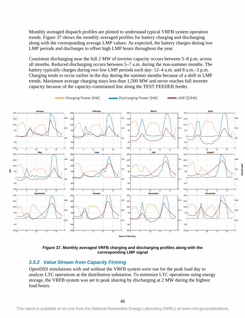
46 This report is available at no cost from the National Renewable Energy Laboratory (NREL) at www.nrel.gov/publications.
Monthly averaged dispatch profiles are plotted to understand typical VRFB system operation trends. Figure 37 shows the monthly averaged profiles for battery charging and discharging along with the corresponding average LMP values. As expected, the battery charges during low LMP periods and discharges to offset high LMP hours throughout the year.
Consistent discharging near the full 2 MW of inverter capacity occurs between 5–8 p.m. across all months. Reduced discharging occurs between 5–7 a.m. during the non-summer months. The battery typically charges during two low LMP periods each day: 12–4 a.m. and 8 a.m.–3 p.m. Charging tends to occur earlier in the day during the summer months because of a shift in LMP trends. Maximum average charging stays less than 1,500 MW and never reaches full inverter capacity because of the capacity-constrained line along the TEST FEEDER feeder.
Figure 37. Monthly averaged VRFB charging and discharging profiles along with the
corresponding LMP signal
3.5.2 Value Stream from Capacity Firming OpenDSS simulations with and without the VRFB system were run for the peak load day to analyze LTC operations at the distribution substation. To minimize LTC operations using energy storage, the VRFB system was set to peak shaving by discharging at 2 MW during the highest load hours.
LMP [$/kW
]
Hours of the Day
Charging Power [kW] Discharging Power [kW] LMP [$/kW]
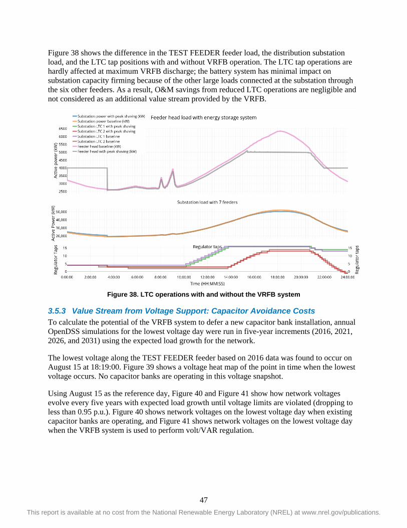
47 This report is available at no cost from the National Renewable Energy Laboratory (NREL) at www.nrel.gov/publications.
Figure 38 shows the difference in the TEST FEEDER feeder load, the distribution substation load, and the LTC tap positions with and without VRFB operation. The LTC tap operations are hardly affected at maximum VRFB discharge; the battery system has minimal impact on substation capacity firming because of the other large loads connected at the substation through the six other feeders. As a result, O&M savings from reduced LTC operations are negligible and not considered as an additional value stream provided by the VRFB.
Figure 38. LTC operations with and without the VRFB system
3.5.3 Value Stream from Voltage Support: Capacitor Avoidance Costs To calculate the potential of the VRFB system to defer a new capacitor bank installation, annual OpenDSS simulations for the lowest voltage day were run in five-year increments (2016, 2021, 2026, and 2031) using the expected load growth for the network.
The lowest voltage along the TEST FEEDER feeder based on 2016 data was found to occur on August 15 at 18:19:00. Figure 39 shows a voltage heat map of the point in time when the lowest voltage occurs. No capacitor banks are operating in this voltage snapshot.
Using August 15 as the reference day, Figure 40 and Figure 41 show how network voltages evolve every five years with expected load growth until voltage limits are violated (dropping to less than 0.95 p.u.). Figure 40 shows network voltages on the lowest voltage day when existing capacitor banks are operating, and Figure 41 shows network voltages on the lowest voltage day when the VRFB system is used to perform volt/VAR regulation.
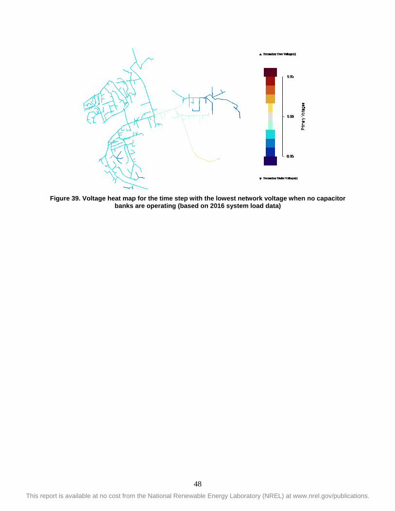
48 This report is available at no cost from the National Renewable Energy Laboratory (NREL) at www.nrel.gov/publications.
Figure 39. Voltage heat map for the time step with the lowest network voltage when no capacitor
banks are operating (based on 2016 system load data)
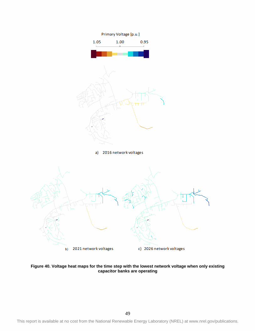
49 This report is available at no cost from the National Renewable Energy Laboratory (NREL) at www.nrel.gov/publications.
Figure 40. Voltage heat maps for the time step with the lowest network voltage when only existing
capacitor banks are operating

50 This report is available at no cost from the National Renewable Energy Laboratory (NREL) at www.nrel.gov/publications.
Figure 41. Voltage heat maps for the time step with the lowest network voltage when the VRFB
system is performing volt/VAR regulation

51 This report is available at no cost from the National Renewable Energy Laboratory (NREL) at www.nrel.gov/publications.
The results show that existing capacitor banks can maintain voltages within bounds along the TEST FEEDER feeder until 2026. Performing volt/VAR regulation using the additional 1 MVAR of reactive capacity from the battery, the VRFB system can defer the installation of a new capacitor bank until 2031.
Assuming that a capacitor costs $56,054 (based on SDG&E rate case testimonies) and discounting it to the calculated out-years using a 6% discount rate, the present value of deferral savings is $7,463. Because the battery can supply 1 MVAR of reactive power without impacting the real power output of the system, this value stream was not included in the optimization but instead added directly as another source of revenue for the VRFB system.
3.5.4 Modeling Shutting Off Auxiliary Pumps when the Battery Is Idle As requested by the battery manufacturer, the optimal dispatch and value stacking results presented in this chapter assume that the electrolyte pump can turn off when the battery is neither charging nor discharging. This impacts only the modeled auxiliary power consumption, not the PCS and storage losses.
Figure 42 shows an example dispatch during the peak load week of 2016. The plot on the left assumes a baseline 18.4-kW auxiliary power consumption when the battery is idle, and the plot on the right shows the results when the battery is allowed to turn off and not draw power when it is not charging nor discharging.
Figure 42. Comparison of optimal dispatch and auxiliary power consumption for two scenarios: (left) 18.4-kW baseline pump consumption when battery is idle and (right) pumps turn off and
draw no power when battery is idle
Total life-cycle costs decrease only marginally, by 0.17%, if the pumps can shut off when the battery is idle. Battery capacity is not affected, and optimal dispatch results are identical because 18.4 kW is a relatively small loss for a 2-MW/8-MWh system. When they are able to shut off, the pumps are switched an average of 6.8 times per day or a little during three on/off cycles.
70 35
0
kW
2000
1000
kW
Sept 25 Sept 27 Sept 29
Sept 25 Sept 27 Sept 29
Charging Discharging Auxiliary Power Auxiliary Power (battery always on) (battery off

52 This report is available at no cost from the National Renewable Energy Laboratory (NREL) at www.nrel.gov/publications.
3.5.5 Value from Line Upgrade Deferral Battery charging is limited by a 2.25-MVA capacity-constrained line between the VRFB installation and the distribution substation. Load less than the capacity-constrained line was monitored at every time step within the optimization to ensure that battery charging never exceeded line limits unless the line upgrade cost was paid. REopt was given the choice of accounting for the upgrade cost to avoid charging limits, but this option was not selected. Because REopt has perfect foresight, the model can optimally dispatch the VRFB system to avoid capacity-constrained periods.
Throughout the year, the line limits restrict battery charging to less than 412 kW–1,618 kW. Figure 43 shows an example of the charging limit as well as the rate at which the VRFB system is charging during the peak load week of 2016. As shown, charging tends to occur at the limit that is allowed to take full advantage of low LMP periods as long as the rate of charge does not set a new system peak and the battery is not at full SOC.
Figure 43. Capacity-constrained line limits for battery charging

53 This report is available at no cost from the National Renewable Energy Laboratory (NREL) at www.nrel.gov/publications.
4 CAISO Market for Energy Storage 4.1 Introduction This section evaluates CAISO’s potential reforms on financial compensation for reactive power support from an asynchronous generating facility, i.e., energy storage system. The existing market and operation rules for reactive power service in CAISO will be explored.
The distribution utility operates within the CAISO balancing authority, which manages the power flow for about 80% of California. As a balancing authority, CAISO operates a transmission control area and balances the generation and load to maintain grid frequency within a specific range. As a market operator, CAISO runs the day-ahead and real-time market for energy and ancillary services and also manages the energy imbalance market among different areas.
The majority of CAISO’s electricity demand is met through the utility-owned or bilaterally procured resources. The remaining unbalance between the generation and demand is handled by day-ahead market and real-time market, as shown in Figure 44.
Figure 44. Electricity power dispatch processes
4.1.1 Market Participants CAISO’s market participants include generators; retail marketers; and utility customers ranging from investor-owned utilities—such as Pacific Gas & Electric, Southern California Edison, and SDG&E—to others such as the Valley Electric Association, to some municipal utilities and financial participants.
4.1.2 Markets in CAISO Day-Ahead Energy Market
The day-ahead energy market is based on forecasts of energy usage, and it procures the bulk of the energy needed to meet California’s electricity demand the following day.

54 This report is available at no cost from the National Renewable Energy Laboratory (NREL) at www.nrel.gov/publications.
Real-Time Energy Market CAISO’s real-time markets include the 15-minute market and 5-minute market, which CAISO uses to manage the differences between the day-ahead forecasted energy loads with actual energy loads. These differences are a function of inaccuracies of forecasts of load and generation as well as unexpected disturbances in the utility grid.
Ancillary Services In addition to the energy market, CAISO has an ancillary service market that includes four services: regulation-up, regulation-down, spinning reserve, and nonspinning reserve.
• Frequency regulation (regulation-up and regulation-down) is used to manage the difference between energy forecasts in the 5 minutes with actual demand in real time. This difference is also called the area control error, which is a small discrepancy because of the inherent nature of forecasts not being completely accurate.
• Spinning reserve is the additional capacity the independent system operator needs to have available to ensure system stability and reliability when the system is suffering from an unexpected event. Spin resources must be synchronized to the grid to be available to provide ramping during a specified range within 10 minutes and be capable of running at least 2 hours.
• Nonspinning reserve is another type of additional capacity the independent system operator procures to ensure system reliability. The nonspinning resource does not need to be synchronized to the grid, but it must be capable of synchronizing with the grid and ramping during a specified range within 10 minutes and be capable of running at least 2 hours.
4.2 Market Participation Model/Resource Model Different resources might choose different participation/resource models to participate in CAISO’s energy and ancillary service market. The participation models include:
• Participating generator (PG)
• Participating load (PL)
• Proxy demand resource (PDR)
• Reliability demand response resource (RDRR)
• Non-generator resource (NGR)
• Pumped storage hydropower (PSH) model.
Considering the different storage scenarios, the corresponding potential participation models are summarized in Table 17

55 This report is available at no cost from the National Renewable Energy Laboratory (NREL) at www.nrel.gov/publications.
Table 17. Participation Model for Different Storage Scenarios
Storage Scenario Participation Model
PG PL PDR RDRR NGR PSH
Transmission connected storage
Stand-alone ES PS
Storage behind the meter of a generating facility
ES PS
WDAT-connected DERs
Stand-alone GEN Pumps ES PS
Behind meter of generating facility
GEN Pumps ES PS
Behind end-use customer meter
GEN Pumps ES PS
Rule 21-connected DERs
Behind end-use customer meter
GEN Pumps Demand
Response
Demand
Response
ES PS
Storage may participate in CAISO markets as an NGR or wholesale demand response product (PDR and RDRR). The VRFB system can fall into the category of interconnected device under wholesale distribution access tariff (WDAT) or interconnected under California’s Rule 21, then NGR, PDR, and RDRR could be the resource model options.
4.2.1 NGRs In 2010, CAISO began an effort to revise its tariff to treat NGRs on a comparable basis with conventional generators. In 2012, CAISO implemented NGR functionality within the wholesale markets. Within the non-generator tariff framework, CAISO developed additional functionality for resources providing regulation services called Regulation Energy Management, or REM. NGR and NGR-REM are defined as follows:
• NGR: A new resource type and model for energy-constrained resources that can operate continuously between generation and load
• NGR-REM: An option for NGRs that provide only regulation services. NGR-REM is proposed to allow NGR resources to bid their capacity more effectively into the independent system operator regulation markets. It allows energy storage to use full capacity to provide grid support services with a shorter time period.
Model NGR resources are modeled as a generator with positive and negative energy. They are constrained by an upper and lower capacity (MW) limit to inject or withdraw energy and are also constrained by an energy (MWh) limit to inject or withdraw energy on a continuous basis. CAISO will use energy limits and SOC values to co-optimize the NGR resource during multiple
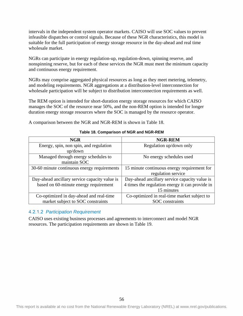
56 This report is available at no cost from the National Renewable Energy Laboratory (NREL) at www.nrel.gov/publications.
intervals in the independent system operator markets. CAISO will use SOC values to prevent infeasible dispatches or control signals. Because of these NGR characteristics, this model is suitable for the full participation of energy storage resource in the day-ahead and real time wholesale market.
NGRs can participate in energy regulation-up, regulation-down, spinning reserve, and nonspinning reserve, but for each of these services the NGR must meet the minimum capacity and continuous energy requirement.
NGRs may comprise aggregated physical resources as long as they meet metering, telemetry, and modeling requirements. NGR aggregations at a distribution-level interconnection for wholesale participation will be subject to distribution interconnection requirements as well.
The REM option is intended for short-duration energy storage resources for which CAISO manages the SOC of the resource near 50%, and the non-REM option is intended for longer duration energy storage resources where the SOC is managed by the resource operator.
A comparison between the NGR and NGR-REM is shown in Table 18.
Table 18. Comparison of NGR and NGR-REM
NGR NGR-REM Energy, spin, non spin, and regulation
up/down Regulation up/down only
Managed through energy schedules to maintain SOC
No energy schedules used
30-60 minute continuous energy requirements 15 minute continuous energy requirement for regulation service
Day-ahead ancillary service capacity value is based on 60-minute energy requirement
Day-ahead ancillary service capacity value is 4 times the regulation energy it can provide in
15 minutes Co-optimized in day-ahead and real-time
market subject to SOC constraints Co-optimized in real-time market subject to
SOC constraints
Participation Requirement CAISO uses existing business processes and agreements to interconnect and model NGR resources. The participation requirements are shown in Table 19.

57 This report is available at no cost from the National Renewable Energy Laboratory (NREL) at www.nrel.gov/publications.
Table 19. Participation Requirement for NGRs
Telemetry Parameters Requirements
Resource instantaneous output, instantaneous SOC, max/min operating limit, resource connectivity status, resource automatic generation control status.
Bidding parameters requirements
Upper charge limit (MWh), lower charge limit (MWh)
Minimum Continuous Energy Ancillary Service Procurement Requirements for NGRs and NGR/REMs
Day-ahead regulation-up/-down 60 min (non-REM)/15 min (REM)
Real-time regulation-up/-down 30 min
Spinning and nonspinning 30 min (non-REM)/NA (REM)
Minimum capacity requirements 500 kW
4.2.2 Demand Response Product PDR was implemented in 2010, and the RDRR implementation was finalized in 2014 after Federal Energy Regulatory Commission ruling and compliance filing delays. The PDR and RDRR products are defined as follows:
• PDR: A load or aggregation of loads that provides demand response services pursuant to a demand response provider agreement between the independent system operator and a demand response provider.
• RDRR: Enables emergency responsive demand response resource participation.
Model Table 20. Participation Options for PDR and RDRR

58 This report is available at no cost from the National Renewable Energy Laboratory (NREL) at www.nrel.gov/publications.
Participation Requirements The participation requirements for PDR and RDRR are shown in Table 21.
Table 21. Participation Requirements for PDR
PDR Participation Requirements
Minimum load curtailment >= 100 kW for energy
Minimum load curtailment >= 500 kW for ancillary services
Allow aggregation to achieve minimum targets
10-kW minimum increments
Telemetry is required for resources >= 10 MW or participating in ancillary services
Scheduling Coordinator Metered Entity
Scan rate = 60 s for PDR; scan rate = 2 s for resources > 10 MW or ancillary services participation at any size (not applicable for spinning reserve participation)
Table 22. Participation Requirements for RDRR
RDRR Participation Requirements
Minimum load curtailment >= 500 kW
Allow aggregation to achieve minimum targets
10-kW minimum increments
Telemetry is not required
Scheduling Coordinator Metered Entity
For Real-Time Reliability Participation
Must be capable of reaching full curtailment within 40 min
May elect to receive discrete dispatches in real time under this option: -Size limited to 50 MW -Cannot participate in day-ahead market
Minimum run time not greater than 1 h
Maximum run time of at least 4 h

59 This report is available at no cost from the National Renewable Energy Laboratory (NREL) at www.nrel.gov/publications.
5 Dynamic Efficiency and Dynamic Loss Modeling 5.1 Data Sampling Several variables were recorded in situ while the VRFB was charged and discharged, including the power losses associated with the PCS, internal battery losses, and parasitic losses corresponding to running the auxiliary electrolyte pumps and cooling system; along with the DC current, DC voltage, SOC, and active power measurements. The DC current, DC voltage, SOC, and active power were recorded for one of the transformers as the VRFB charged and discharged while operating at various active power settings (Figure 45). Hence, the measured active power is for half of the total capacity of the VRFB. All measured data are reported in this way, whereas all simulated results (Section 5.4) are reported with both transformers together, i.e., twice the measured data. The three loss vectors aggregate to contribute to the total system losses and ultimately decrease the charging and discharging efficiencies. This section discusses both the dynamic efficiencies and the dynamic losses.
Figure 45. VRFB state variables for charging and discharging at 1,000 kW, 750 kW, 500 kW, 372
kW, and 300 kW, respectively
5.2 Dynamic Efficiency Modeling We calculate the energy efficiency while charging and discharging. The three loss vectors—PCS losses, internal battery losses, and parasitic losses—decrease the efficiency. These are measured at the VRFB, whereas the active power is measured slightly farther down the line. The power measurements were recorded at constant time intervals. Thus, the energy efficiency can be calculated directly from the power measurements. We ignore the line losses, which are negligible given the proximity of the VRFB to the point at which active power is measured. Thus, as the VRFB is charged, the active power is measured before the losses occur. Therefore, given our experimental data and collection method, the charging efficiency is defined as:
𝜂𝜂𝐶𝐶ℎ𝑟𝑟𝑉𝑉𝑉𝑉𝑉𝑉𝑈𝑈 ≡|𝑃𝑃𝑉𝑉𝑉𝑉𝑉𝑉𝑈𝑈|
|𝑃𝑃𝐼𝐼𝑚𝑚| =|𝑃𝑃𝐼𝐼𝑚𝑚| − (𝐿𝐿𝑃𝑃𝐶𝐶𝑃𝑃 + 𝐿𝐿𝐼𝐼𝑚𝑚𝑏𝑏𝑟𝑟𝑟𝑟𝑚𝑚𝑏𝑏𝑙𝑙+𝐿𝐿𝑃𝑃𝑏𝑏𝑟𝑟𝑏𝑏𝑑𝑑𝑚𝑚𝑏𝑏𝑚𝑚𝑑𝑑)
|𝑃𝑃𝐼𝐼𝑚𝑚|
As the VRFB is discharged, the active power is measured after the losses occur. Therefore, the discharging efficiency is defined as:
𝜂𝜂𝐷𝐷𝑚𝑚𝑑𝑑𝑉𝑉𝑉𝑉𝑉𝑉𝑈𝑈 ≡|𝑃𝑃𝑂𝑂𝑂𝑂𝑏𝑏|
|𝑃𝑃𝑉𝑉𝑉𝑉𝑉𝑉𝑈𝑈| =|𝑃𝑃𝑂𝑂𝑂𝑂𝑏𝑏|
(𝐿𝐿𝑃𝑃𝐶𝐶𝑃𝑃 + 𝐿𝐿𝐼𝐼𝑚𝑚𝑏𝑏𝑟𝑟𝑟𝑟𝑚𝑚𝑏𝑏𝑙𝑙+𝐿𝐿𝑃𝑃𝑏𝑏𝑟𝑟𝑏𝑏𝑑𝑑𝑚𝑚𝑏𝑏𝑚𝑚𝑑𝑑) + |𝑃𝑃𝑂𝑂𝑂𝑂𝑏𝑏|
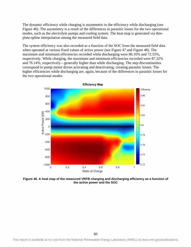
60 This report is available at no cost from the National Renewable Energy Laboratory (NREL) at www.nrel.gov/publications.
The dynamic efficiency while charging is asymmetric to the efficiency while discharging (see Figure 46). The asymmetry is a result of the differences in parasitic losses for the two operational modes, such as the electrolyte pumps and cooling system. The heat map is generated via thin-plate-spline interpolation among the measured field data.
The system efficiency was also recorded as a function of the SOC from the measured field data when operated at various fixed values of active power (see Figure 47 and Figure 48). The maximum and minimum efficiencies recorded while discharging were 86.16% and 72.55%, respectively. While charging, the maximum and minimum efficiencies recorded were 87.32% and 76.14%, respectively—generally higher than while discharging. The step discontinuities correspond to pump motor drives activating and deactivating, creating parasitic losses. The higher efficiencies while discharging are, again, because of the differences in parasitic losses for the two operational modes.
Figure 46. A heat map of the measured VRFB charging and discharging efficiency as a function of
the active power and the SOC

61 This report is available at no cost from the National Renewable Energy Laboratory (NREL) at www.nrel.gov/publications.
Figure 47. Measured discharge efficiency against the SOC when operated for various fixed values
of active power
Figure 48. Measured charging efficiency against the SOC when operated for various fixed values
of active power
The parasitic losses significantly impact the system efficiency; the most significant of these is the pump motor drives. Given the existing pumping scheme, when a motor drive is activated, the system efficiency might rapidly drop by more than 5%, as shown while charging at 500 kW and with an SOC of more than 80%. The system efficiency could potentially be improved by optimizing the pumping controller to minimize these losses while charging and discharging the VRFB.
Still, the utility-scale VRFB features charging and discharging efficiencies that are significantly higher than those for smaller capacity units. This is primarily because of the larger motor drives on the electrolyte pumps and cooling systems. Larger motors have higher partial-load efficiencies than smaller motor drives. Therefore, the parasitic losses, as a percentage of the active power, detract less from the efficiency of the utility-scale VRFB than for smaller capacity units, which require smaller motor capacities.

62 This report is available at no cost from the National Renewable Energy Laboratory (NREL) at www.nrel.gov/publications.
The higher efficiency for the utility-scale VRFB, and long cycle life, suggest that this technology has reached a level of maturity that has not been previously demonstrated. Efficiencies are useful for comparing one storage technology to another, but the losses that contribute to the dynamic efficiencies can impact the operation strategy of the technology. Further, the accuracy of the loss modeling can impact the operation strategy. Therefore, we also model the losses as a function of the VRFB operating state variables.
5.3 Dynamic Loss Modeling Techniques The most relevant operating state variables for determining the grid support strategies are the SOC and the active power. For this reason, each of the subsequent loss models are a function of these variables. Toward modeling the total system losses of the VRFB, we employ several techniques and evaluate the accuracy of each method. First, we employ a simple triangular interpolation between the measured field data instances. This simple interpolating technique fails to capture any nonlinearities between the total system losses and the operating state variables, so we explore several techniques, each with increasing complexity, to capture these nonlinearities. A composite quadratic function of the SOC and active power is explored. Additionally, we model the total system losses as a bivariate quadratic function of the VRFB operating state variables. Finally, we train a nonlinear artificial neural network (ANN) to predict the system losses as a function of the VRFB SOC and active power.
5.3.1 Metrics for Evaluating Model Accuracy Each modeling method is evaluated for accuracy as its ability to predict the total system losses from the VRFB operating state variables. The root mean square error (RMSE) and the maximum error are calculated to gauge the accuracy of each model. Finally, the coefficient of determination, or r-squared statistic, is calculated to gauge how well the variance in the total system losses are explained by the variance among the operating state variables:
RMSE = �∑ (yi − y�i)2ni=1
n (3)
Max Error = max{|yi − y�i |} (4)
R2 = 1 −∑ (yi − y�i)2ni=1
∑ (yi − y�i)2ni=1
(5)
where yi are the measured losses, y�i are the modeled losses, �yi is the mean measured losses, and n is the number of measured data points.
5.3.2 Triangular Interpolation To model total system losses, we used field data provided by battery manufacturer. Figure 49 shows a polytope encompassing the field data points. A system of equations was generated from the polytope.
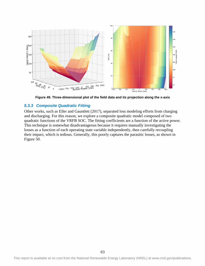
63 This report is available at no cost from the National Renewable Energy Laboratory (NREL) at www.nrel.gov/publications.
Figure 49. Three-dimensional plot of the field data and its projection along the x-axis
5.3.3 Composite Quadratic Fitting Other works, such as Eller and Gauntlett (2017), separated loss modeling efforts from charging and discharging. For this reason, we explore a composite quadratic model composed of two quadratic functions of the VRFB SOC. The fitting coefficients are a function of the active power. This technique is somewhat disadvantageous because it requires manually investigating the losses as a function of each operating state variable independently, then carefully recoupling their impact, which is tedious. Generally, this poorly captures the parasitic losses, as shown in Figure 50.

64 This report is available at no cost from the National Renewable Energy Laboratory (NREL) at www.nrel.gov/publications.
. Figure 50. Composite model for loss as a function of the active power and SOC
5.3.4 Bivariate Quadratic Fitting The total system losses seem to be well approximated by a quadratic function of the operating state (see Figure 51). The advantage is that the fitting coefficients can be easily found via any nonlinear solver. This technique also poorly captures the parasitic losses.
State of
Charge [%]
100
0
50
-1000
Composite Model of Losses
100
50
150
Tota
l Los
ses
[kW
]
-500
200
Active Power [kW]
250
0
300
50001000
Measured Data
Composite Model

65 This report is available at no cost from the National Renewable Energy Laboratory (NREL) at www.nrel.gov/publications.
Figure 51. Bivariate model of losses against active power and SOC
5.3.5 Nonlinear ANN Model The underlying relationship between the total system losses and the VRFB operating state variables is not known a priori. In this situation, a model-free fitting technique, such as an ANN model, lends itself well to the problem of predicting the total system losses. Model-free fitting is a technique wherein a meta model, such as a bivariate quadratic model, is not assumed in advance. Instead, the ANN is trained on the data using the batch back-propagation algorithm. The ANN is made nonlinear by introducing a hidden layer and is free to translate by some reference constant by introducing a bias weight and a virtual bias node as described by Eyer and Corey (2010, 5). The basic structure of the ANN is shown in Figure 52. The number of hidden nodes needed to accurately model the data is not known, so a sensitivity analysis is performed to investigate the relationship between the accuracy of the model and the number of hidden nodes that are included.
1
0
Bivariate Model of LossesLosses vs Active Power, SOC
50
-1000
100
State of Charge
0.5
150
Tota
l Los
ses
[kW
]
-500
200
250
Active Power [kW]
0
300
50001000
Losses vs Active Power,SOC
Measured Data

66 This report is available at no cost from the National Renewable Energy Laboratory (NREL) at www.nrel.gov/publications.
Figure 52. Basic structure of the nonlinear neural network. One input layer with a virtual bias node, one hidden layer, and one output layer are used. The w(i,h) and x(h) terms denote the weights on the links between nodes, which are found via the back-propagation algorithm.
The back-propagation algorithm iteratively modifies the weights between nodes in the neural network to improve the model accuracy. If the model accuracy, as measured by the sum-of-squares error, does not improve by more than some threshold, then the algorithm terminates after the current iteration. Additionally, a maximum iteration limit is imposed to prevent endless looping. Here, we use 90% of the measured data to train the ANN, and the remaining 10% is used for cross-validation. The ANN model is also advantageous because in this case the parasitic losses are highly nonlinear.
Figure 53. ANN model of losses against active power and SOC
1
Artificial Neural Network Model of Losses
0
50
-1000
100
State of Charge
0.5
150
Tota
l Los
ses
[kW
]
200
-500
250
300
Active Power [kW]
0500
01000
Measured Data
ANN Model
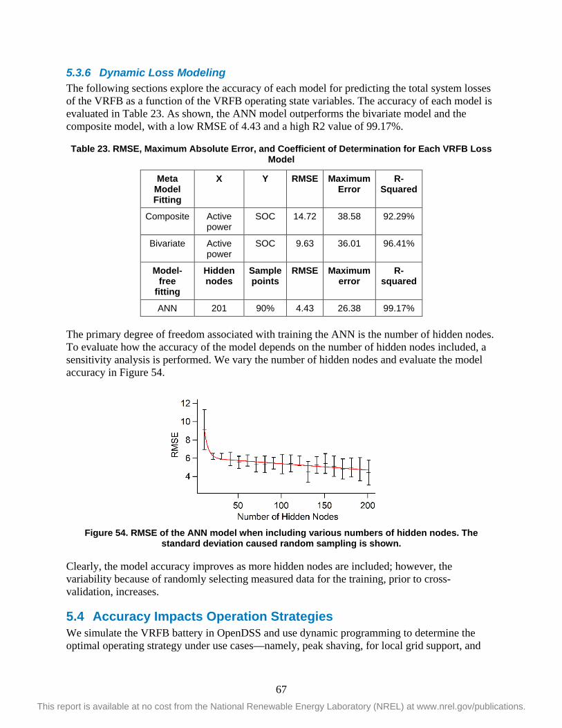
67 This report is available at no cost from the National Renewable Energy Laboratory (NREL) at www.nrel.gov/publications.
5.3.6 Dynamic Loss Modeling The following sections explore the accuracy of each model for predicting the total system losses of the VRFB as a function of the VRFB operating state variables. The accuracy of each model is evaluated in Table 23. As shown, the ANN model outperforms the bivariate model and the composite model, with a low RMSE of 4.43 and a high R2 value of 99.17%.
Table 23. RMSE, Maximum Absolute Error, and Coefficient of Determination for Each VRFB Loss Model
Meta Model Fitting
X Y RMSE Maximum Error
R-Squared
Composite Active power
SOC 14.72 38.58 92.29%
Bivariate Active power
SOC 9.63 36.01 96.41%
Model-free
fitting
Hidden nodes
Sample points
RMSE Maximum error
R-squared
ANN 201 90% 4.43 26.38 99.17%
The primary degree of freedom associated with training the ANN is the number of hidden nodes. To evaluate how the accuracy of the model depends on the number of hidden nodes included, a sensitivity analysis is performed. We vary the number of hidden nodes and evaluate the model accuracy in Figure 54.
Figure 54. RMSE of the ANN model when including various numbers of hidden nodes. The
standard deviation caused random sampling is shown.
Clearly, the model accuracy improves as more hidden nodes are included; however, the variability because of randomly selecting measured data for the training, prior to cross-validation, increases.
5.4 Accuracy Impacts Operation Strategies We simulate the VRFB battery in OpenDSS and use dynamic programming to determine the optimal operating strategy under use cases—namely, peak shaving, for local grid support, and

68 This report is available at no cost from the National Renewable Energy Laboratory (NREL) at www.nrel.gov/publications.
energy arbitrage—to maximize the value of the VRFB. The various loss models are incorporated into OpenDSS simulations of the VRFB and feeder. For peak shaving, the VRFB charges or discharges to limit the load on the feeder to less than some threshold. For energy arbitrage, the VRFB charges and discharges to maximize the value of the energy supplied by the VRFB. Day-ahead LMP prices are obtained for the feeder and are incorporated into the problem formulation to be solved via dynamic programming. Relying on historical data spanning 1 year, the LMP signal corresponding to the most typical day was identified. The most typical day has a mean value and variance most like the mean value and a variance of the historical data set. This approach was inspired by the method from Sandia National Laboratories for generating typical meteorological year data sets [3]. The optimal operating schedule for energy arbitrage for the typical day is then obtained using the backward value iteration algorithm. To improve the speed of the algorithm, state memorization is imposed.
5.4.1 Accuracy Impacts Operation Strategies Local Grid Support: Peak Shaving
We compare the various VRFB loss models by running a base-loading/peak-shaving simulation scenario in OpenDSS using a real feeder. The simulation is run for a day with the active power lower limits, 𝑃𝑃𝑙𝑙𝑏𝑏, and upper limits, Pub, at the feeder head set at 3,500 kW and 4,500 kW, respectively (see Figure 55).
Figure 55. Substation power in KW
The VRFB charges as the substation power falls below 𝑃𝑃𝑙𝑙𝑏𝑏 and discharges as demand exceeds the upper active power bound, 𝑃𝑃𝑂𝑂𝑏𝑏. The active power output from the VRFB peaks at 20% of 𝑃𝑃𝑟𝑟𝑏𝑏𝑏𝑏𝑟𝑟𝑑𝑑 while charging and about 20% of Prated while discharging (see Figure 56).
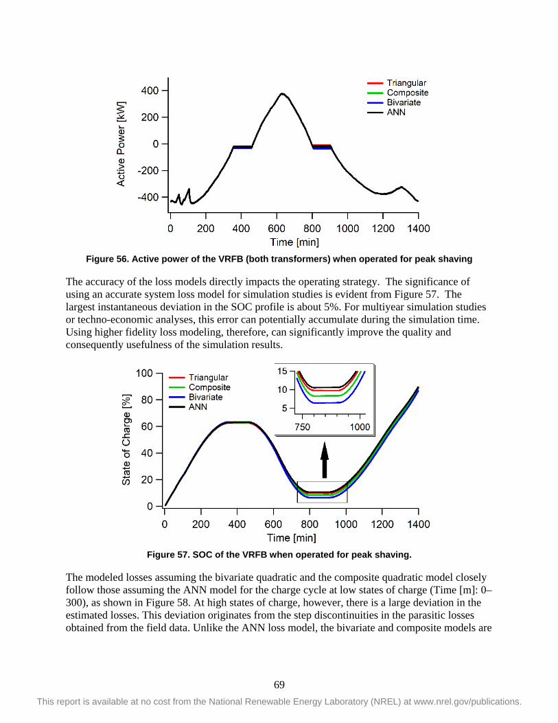
69 This report is available at no cost from the National Renewable Energy Laboratory (NREL) at www.nrel.gov/publications.
Figure 56. Active power of the VRFB (both transformers) when operated for peak shaving
The accuracy of the loss models directly impacts the operating strategy. The significance of using an accurate system loss model for simulation studies is evident from Figure 57. The largest instantaneous deviation in the SOC profile is about 5%. For multiyear simulation studies or techno-economic analyses, this error can potentially accumulate during the simulation time. Using higher fidelity loss modeling, therefore, can significantly improve the quality and consequently usefulness of the simulation results.
Figure 57. SOC of the VRFB when operated for peak shaving.
The modeled losses assuming the bivariate quadratic and the composite quadratic model closely follow those assuming the ANN model for the charge cycle at low states of charge (Time [m]: 0–300), as shown in Figure 58. At high states of charge, however, there is a large deviation in the estimated losses. This deviation originates from the step discontinuities in the parasitic losses obtained from the field data. Unlike the ANN loss model, the bivariate and composite models are

70 This report is available at no cost from the National Renewable Energy Laboratory (NREL) at www.nrel.gov/publications.
unable to cater to these step discontinuities. For lower values of active power dispatch, the composite model fits the field better compared to the bivariate model.
Figure 58. Modeled losses (both transformers) of VRFB when operated for peak shaving
Because of the differences in the dynamic losses, the calculated dynamic efficiencies also feature significant differences, especially when the VRFB is discharging, or for very high states of charge (see Figure 59). Focusing on the dynamic efficiencies calculated assuming the most accurate loss model, the ANN, it is clear that when being operated for peak shaving and subject to the constraints on this substation, the dynamic efficiency of the VRFB is generally suboptimal.
Figure 59. Dynamic efficiency of the VRFB when operated for peak shaving, assuming each loss
model
Maximizing Value Generation: Energy Arbitrage The accuracy of the loss model is also paramount when the VRFB is operated for energy arbitrage. Figure 60–Figure 65 demonstrate how the loss model can significantly impact the

71 This report is available at no cost from the National Renewable Energy Laboratory (NREL) at www.nrel.gov/publications.
optimal operating strategy for the VRFB and therefore the value generated during a single day. Generally, the reduced accuracy of the triangular interpolation, the composite model, and the bivariate model, relative to the ANN, result in errors when estimating the cumulative value of the VRFB during the most typical LMP day. The LMP signal at the feeder on the most typical day of 2017 is shown in Figure 60. Clearly, the optimal operating strategy is impacted by the accuracy of the loss model being employed (see Figure 61).
Figure 60. LMP signal at the feeder on the most typical day
Figure 61. Optimal active power (both transformers) for the VRFB on the most typical day, solved
assuming each VRFB loss model
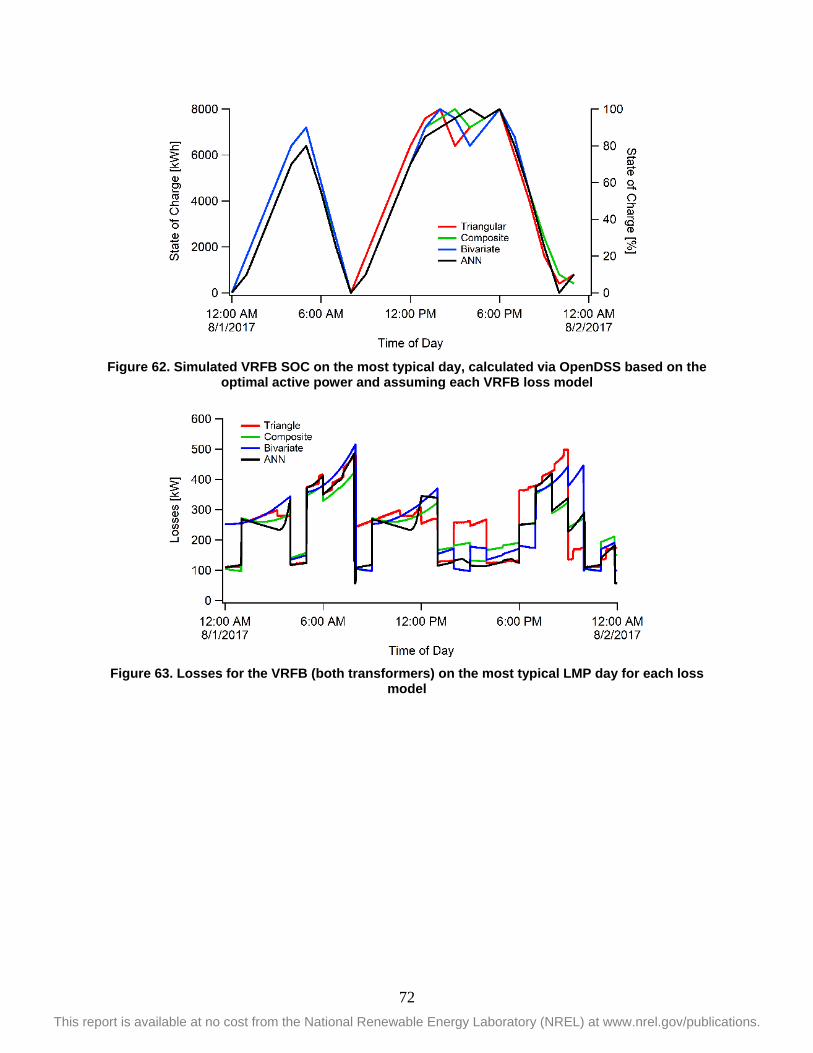
72 This report is available at no cost from the National Renewable Energy Laboratory (NREL) at www.nrel.gov/publications.
Figure 62. Simulated VRFB SOC on the most typical day, calculated via OpenDSS based on the
optimal active power and assuming each VRFB loss model
Figure 63. Losses for the VRFB (both transformers) on the most typical LMP day for each loss
model

73 This report is available at no cost from the National Renewable Energy Laboratory (NREL) at www.nrel.gov/publications.
Figure 64. Dynamic efficiency for the VRFB on the most typical LMP day, calculated assuming
each loss model
Most importantly, the expected cumulative value generated by the VRFB, when employing the various loss models, can be significantly different by the end of the day (see Figure 65). When employing the composite quadratic loss model, the expected value generated by the VRFB is overestimated by more than 9% relative to the value obtained when employing the more accurate ANN. This overestimate of the generated value would persist for every other day of the year, and during the life cycle of the battery, as long as the composite loss model was employed. We show the simulated efficiency as a path through the efficiency heat map in Figure 66.
Figure 65. Expected cumulative value generated by the VRFB on the most typical day, assuming
each VRFB loss model

74 This report is available at no cost from the National Renewable Energy Laboratory (NREL) at www.nrel.gov/publications.
Figure 66. Trajectory of the VRFB operating states through the efficiency space when the battery
is operated for energy arbitrage (white) and peak shaving (magenta), assuming the ANN loss model (A single transformer is shown.)

75 This report is available at no cost from the National Renewable Energy Laboratory (NREL) at www.nrel.gov/publications.
6 Operational Planning and Field-Testing 6.1 Scope of Testing At the request of the battery manufacturer, we assisted in operational testing of the VRFB system for a 1-week period in April. This testing included three different approaches to dispatching the battery:
1. Heuristic peak shaving/base-loading: This strategy selects set points that the VRFB attempts to maintain for multiple hours. One set point is selected for peak shaving (battery discharging) and is applied during high-load periods of day, and a second set point is selected for base-loading (battery charging) during low-load periods. This strategy requires a load forecast to identify the set points and associated periods of the day in which to implement them. A heuristic method was also used to attempt to align the set points with high/low LMP hours.
2. Cost-optimal arbitrage: This strategy selects multiple set points throughout the day, with a goal of optimizing the revenue that the battery can achieve from the day-ahead LMP market. A total of eight distinct power set points—and associated start times—can be input to the PCS during a given period. This strategy uses the REopt model to select the eight (or fewer) optimal set points to maximize revenue from the day-ahead LMP markets. No load forecast is required for this strategy.
3. Hybrid peak shaving and optimal arbitrage: This strategy uses the same PCS control strategy as the cost-optimal arbitrage (max of eight power set points) and optimizes revenue from the LMP market while ensuring that the load on the feeder does not exceed a prescribed power limit. This strategy uses the REopt model to select the set points and uses a load forecast to inform the peak-shaving objective.
The peak-shaving/base-loading strategy was executed from April 2–4, the cost-optimal arbitrage strategy was executed from April 4–5, and the hybrid strategy was executed from April 5–6.
Note that two of the three strategies require a forecast of the feeder load to execute the dispatch strategy. To achieve the load prediction, we trained an ANN to predict the feeder load as a function of the meteorological forecasts. The meteorological forecasts, and the subsequent feeder load forecasts, extended through an 18-hour-ahead time horizon at an hourly resolution. The true feeder load and the operating state variables of the VRFB were continuously monitored during the week of testing to enable comparisons with the expected feeder load obtained from the load forecasts and the resultant operational plan.
6.2 ANN Model for Feeder Load Forecasting This section discusses how the ANN model for the feeder load was developed and evaluated for accuracy.
6.2.1 Historical Feeder Load Data We received load data from the feeder, with the impact of the battery included, spanning the months of January and February on a 10-second resolution from the distribution utility. These data were downsampled to an hourly resolution by averaging across each hour. The data

76 This report is available at no cost from the National Renewable Energy Laboratory (NREL) at www.nrel.gov/publications.
corresponding to the feeder load with the impact of the battery were serially complete. Additionally, we received feeder load data without the impact of the battery included and spanning the same time frame on an hourly resolution from Sumitomo. The data corresponding to the feeder load without the impact of the battery were not serially complete and featured missing data in rare cases. The missing data were represented in the time series as null values.
6.2.2 High-Resolution Rapid Refresh Meteorological Data The primary input variables used in training the ANN were meteorological variables. These variables were selected because temperature, solar irradiance, and other climatic variables have a large impact on both building electrical loads and solar PV performance on the feeder. For this analysis, we selected the High-Resolution Rapid Refresh (HRRR) data set that is provided by the National Center for Environmental Prediction on a 3-km by 3-km grid for the entire continental United States.2 The HRRR data sat was selected because it is the only publicly available data set known to the authors that provides hourly forecast data for solar radiation as well as a wide variety of additional meteorological variables.
The variables pulled from the HRRR data were atmospheric pressure (surface level), temperature (surface level and 2 m aboveground), dewpoint temperature (2 m aboveground), specific humidity (2 m aboveground), and downward shortwave radiation flux (surface level). These variables were pulled for the area bounded by the following grid of latitudes between 32.668 and 32.67 and for longitudes between -116.98 and -116.97.
6.2.3 Singular ANN Model Training A multilayer perceptron network, a class of feedforward ANNs, was trained to predict the feeder load without the impact of the battery as a function of the HRRR data. The network was composed of three layers: the input layer, the hidden layer to allow for nonlinearities in the model, and the output layer; see Figure 67. The input layer consisted of 19 hourly values for each of the six weather variables for a total of 114 inputs. The 19 hourly values correspond to the current hour and the 18-hourly forecasted values. The hidden layer consisted of 2,000 hidden nodes, a number selected after a sensitivity analysis that indicates there are diminishing returns on accuracy with a linear increase in time, as shown in Figure 68. Thus, 2,000 hidden nodes yield high performance while not requiring unnecessary time to train the network. The output is the feeder load and contains 19 hourly values, including the current hour and the next 18-hourly values.
2 http://www.nco.ncep.noaa.gov/pmb/products/hrrr/, accessed April 21, 2018

77 This report is available at no cost from the National Renewable Energy Laboratory (NREL) at www.nrel.gov/publications.
Figure 67. General structure of the ANN model
Figure 68. (Left) Adjusted R-squared value of the ANN model as a function of the number of
hidden nodes and (right) training time for the ANN as a function of the hidden nodes
6.2.4 Multiple ANN Model Training Training an ANN involves randomly selecting initial conditions for the weighting parameters that interrelate the nodes in the network. Therefore, each time a network is trained on the same data set, different initial conditions will be used, and the resulting network will be slightly different after the training is complete. Further, the final trained network will feature some error relative to the training data and some bias error relative to “live” data outside of the training set. By training multiple networks of identical form on the same data set and taking the mean of their outputs, the bias error can be reduced on average. For this reason, we trained 50 ANNs of identical form against the training data set and took the mean of their outputs, as shown in Figure 69.
Historical HRRR Data
Historical Load Data
Hidden Nodes (N=2000 in
Input Nodes (19 hourly values for 6 weather variables , n=144 inputs)
ANN (simplified graphic)
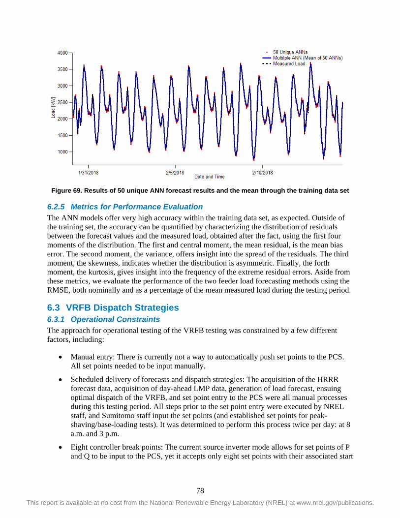
78 This report is available at no cost from the National Renewable Energy Laboratory (NREL) at www.nrel.gov/publications.
Figure 69. Results of 50 unique ANN forecast results and the mean through the training data set
6.2.5 Metrics for Performance Evaluation The ANN models offer very high accuracy within the training data set, as expected. Outside of the training set, the accuracy can be quantified by characterizing the distribution of residuals between the forecast values and the measured load, obtained after the fact, using the first four moments of the distribution. The first and central moment, the mean residual, is the mean bias error. The second moment, the variance, offers insight into the spread of the residuals. The third moment, the skewness, indicates whether the distribution is asymmetric. Finally, the forth moment, the kurtosis, gives insight into the frequency of the extreme residual errors. Aside from these metrics, we evaluate the performance of the two feeder load forecasting methods using the RMSE, both nominally and as a percentage of the mean measured load during the testing period.
6.3 VRFB Dispatch Strategies 6.3.1 Operational Constraints The approach for operational testing of the VRFB testing was constrained by a few different factors, including:
• Manual entry: There is currently not a way to automatically push set points to the PCS. All set points needed to be input manually.
• Scheduled delivery of forecasts and dispatch strategies: The acquisition of the HRRR forecast data, acquisition of day-ahead LMP data, generation of load forecast, ensuing optimal dispatch of the VRFB, and set point entry to the PCS were all manual processes during this testing period. All steps prior to the set point entry were executed by NREL staff, and Sumitomo staff input the set points (and established set points for peak-shaving/base-loading tests). It was determined to perform this process twice per day: at 8 a.m. and 3 p.m.
• Eight controller break points: The current source inverter mode allows for set points of P and Q to be input to the PCS, yet it accepts only eight set points with their associated start

79 This report is available at no cost from the National Renewable Energy Laboratory (NREL) at www.nrel.gov/publications.
times. Because we were scheduling the battery twice per day, this limited the number of times we could change the set point of the VRFB.
We see a significant opportunity to streamline and automate this entire process. This would provide the benefit of continuously updating the load forecast by pulling the HRRR data once every hour (instead of relying on hours-ahead forecasts in some cases during the twice per day testing). It would also allow for more continuous updating of the SOC of the VRFB for the LMP optimization and could enable participation in real-time markets.
6.4 Results In this section, we discuss the results of the forecasting during the week of field-testing. In practice, the single ANN forecast method was applied for the first stage of the testing: peak shaving/base-loading. Then, during both subsequent stages, the multiple ANN method was applied. Here, we show the results of both methods applied throughout the full week of testing.
6.4.1 Load Forecasting Results The rolling forecast obtained from the singular ANN method, along with the measured load, is shown in Figure 70. As each new forecast was generated, it superseded the existing forecast. The series of forecast data used in practice is called the net forecast.
Figure 70. Rolling forecast for the singular ANN method. The net forecast is shown along with the
measured feeder load.
The rolling forecast obtained from the multiple ANN method along with the measured load and the net forecast is shown in Figure 71.
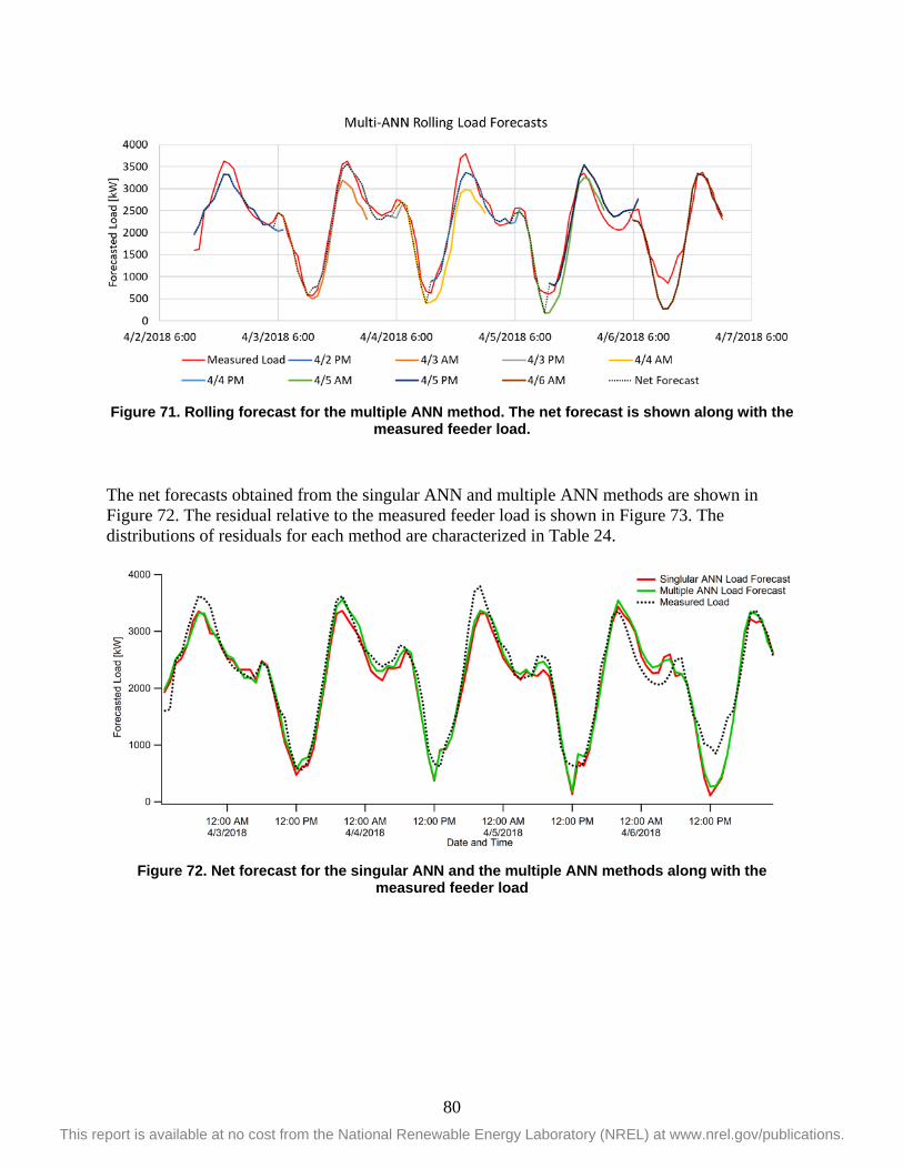
80 This report is available at no cost from the National Renewable Energy Laboratory (NREL) at www.nrel.gov/publications.
Figure 71. Rolling forecast for the multiple ANN method. The net forecast is shown along with the
measured feeder load.
The net forecasts obtained from the singular ANN and multiple ANN methods are shown in Figure 72. The residual relative to the measured feeder load is shown in Figure 73. The distributions of residuals for each method are characterized in Table 24.
Figure 72. Net forecast for the singular ANN and the multiple ANN methods along with the
measured feeder load

81 This report is available at no cost from the National Renewable Energy Laboratory (NREL) at www.nrel.gov/publications.
Figure 73. Residual errors relative to the measured feeder load of the net forecasts obtained from
the singular ANN and multiple ANN methods
Generally, the multiple ANN forecasting method resulted in better performance with smaller nominal RMSE and percentage RMSE than the singular ANN method. Additionally, the mean residual was smaller and the distributions were tighter, albeit similarly skewed, but featured less extreme residuals than the singular ANN forecast method, as is summarized in Table 24.
Table 24. Summary of the Accuracy of the Singular ANN and Multiple ANN Feeder Load Forecasting Methods.
Metric Single ANN
Multiple ANN
Average actual 2226.80 2226.80
RMSE 272.22 247.04
% RMSE 12.22% 11.09%
Mean of residuals 111.62 48.47
Variance of residuals 61529.13 58656.99
Std. Dev. of residuals 248.0507 242.1920
Skewness of residuals 0.2203 0.2599
Kurtosis of residuals 0.5706 0.3268
6.4.2 Optimal Dispatch Results From 4 p.m. on April 4 to 4 p.m. on April 6, the VRFB was put into current source inverter mode and eight set points were entered into the PCS two times per day (at 8 a.m. and 4 p.m.). During this time, the REopt model was used to optimize the set points of the VRFB. The following modifications were made to the optimization model to accommodate the real-time testing formulation:
• Charging the system was capped at 1,620 kW, and discharging was capped at 1,960. (These limits were set because of site load limits based on conductor ratings.)

82 This report is available at no cost from the National Renewable Energy Laboratory (NREL) at www.nrel.gov/publications.
• The optimization model was scaled down to perform a 24-hour optimization.
• The optimization was constrained to select only eight set points within the current scheduling period (either 8 a.m.–4 p.m. or 4 p.m.–8 a.m. on the following day)
• For the 24-hour period from 4 p.m. on April 5 to 4 p.m. on April 6, a peak limit constraint was added to the model such that the feeder load (including charging the VRFB) was forced to remain under that limit. This was set at 3,000 kW for that period.
Figure 74 shows the comparison of active power from the PCS and the optimal dispatch provided by the REopt model. Note that the two signals—commanded output and actual output—match extremely well throughout the testing period (with one exception midday on April 5). The one period in which the signals do not match closely is because the SOC of the system hit zero during that hour (see the dashed line in the figure), and the battery was not able to execute this command for the full period. The most likely reason for the VRFB reaching zero SOC prior to expected full discharge in the optimization model is that the expected SOC at the beginning of operation was 81% but the actual SOC was 71%; therefore, less capacity was available than the model expected, resulting in a power discharge setting that was higher than physically achievable. If we exclude that hour from consideration, the percentage error between command and actual output was ~0.2%.
Figure 74. VRFB dispatch during optimal dispatch
During the hybrid cost-optimal and peak-shaving test period (4 p.m. on April 5 to 4 p.m. on April 6), the model was constrained to limit feeder load to less than 3,000 kW. It then optimized the dispatch schedule to maximize revenue from arbitrage in the LMP market. The results from this dispatch are shown in Figure 75. It is clear that the load without the VRFB would have reached ~3,400 kW during the late afternoon on April 5, yet with the optimized dispatch the feeder load was kept well below that target during those hours and exceeded the target of 3,000 kW by only 89 kW when our forecasting results showed a slightly lower expected feeder loading. Note also that the VRFB was dispatched to take advantage of discharging at high LMP periods (while observing the feeder peak limit set in the model).
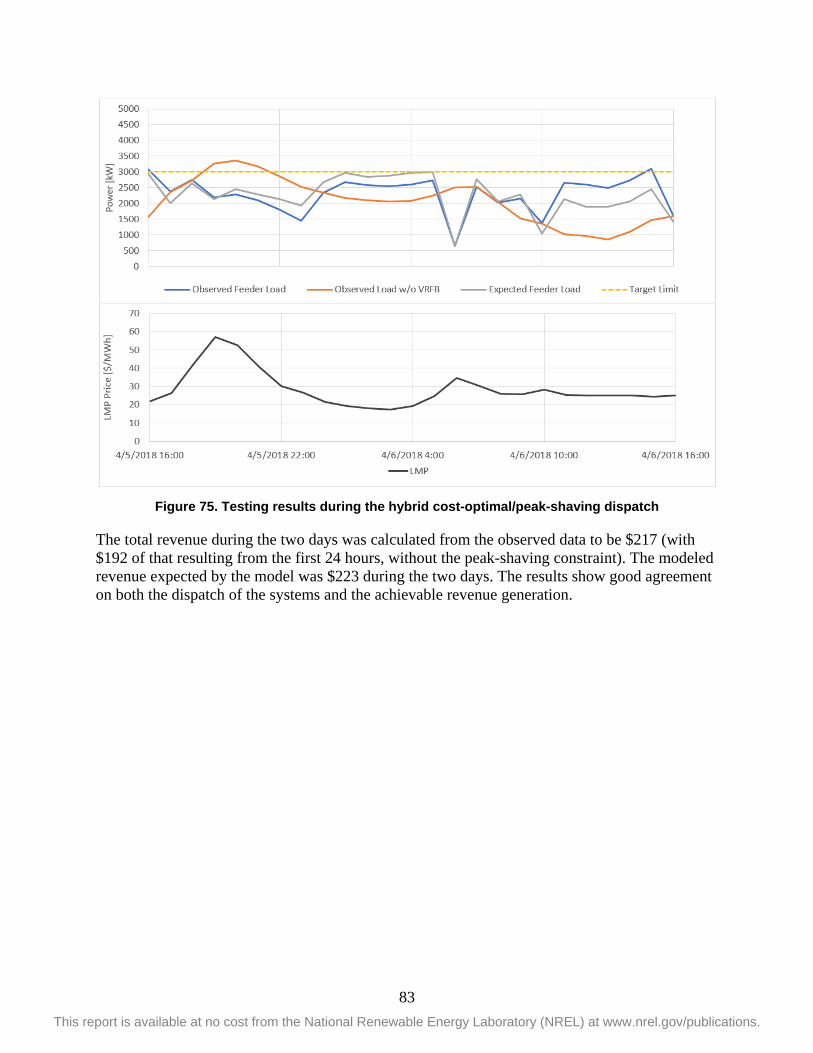
83 This report is available at no cost from the National Renewable Energy Laboratory (NREL) at www.nrel.gov/publications.
Figure 75. Testing results during the hybrid cost-optimal/peak-shaving dispatch
The total revenue during the two days was calculated from the observed data to be $217 (with $192 of that resulting from the first 24 hours, without the peak-shaving constraint). The modeled revenue expected by the model was $223 during the two days. The results show good agreement on both the dispatch of the systems and the achievable revenue generation.

84 This report is available at no cost from the National Renewable Energy Laboratory (NREL) at www.nrel.gov/publications.
7 Conclusions and Remarks Several possible value streams from a VRFB energy storage system were evaluated in this project, with particular focus on local distribution support. Value streams achievable from directly participating in bulk energy markets were not considered in this report. Generally, value from battery energy storage systems are multifold. The battery applications in this project focus on providing distribution system support services as follows:
• Peak shaving: Energy storage charges during low-load periods and discharges during high-load periods to reduce the peak demand on the feeder during the highest loading condition.
• Capacity firming: The objective of capacity firming is to use storage to smooth the output of intermittent renewable energy generation. Storage is able to react quickly to compensate for rapid fluctuations in output, resulting in reduced ramping and a more consistent, less variable load on the system.
• Voltage support: Energy storage can also provide voltage support to maintain feeder voltages within acceptable bounds, typically ±5% of nominal. For sensitive electric appliances and electronics, it is important that voltage is supplied within these limits. Utilities typically install capacitor banks or voltage regulators to boost the voltage at the end of a line. With power electronics capable of injecting and absorbing both real and reactive power at different rates, energy storage is now able to provide the same services.
• Energy arbitrage: Energy storage is charged during off-peak hours and discharged during peak hours to take advantage of the price difference in electricity across time periods. The revenue obtained is the price differential between buying and selling electrical energy minus the cost of losses during the full charge/discharge cycle.
The economics of using the VRFB system to provide grid support functions was evaluated via a combination of OpenDSS simulations and optimizations through a mixed-integer linear program using NREL’s REopt model. A novel schematic was developed to assess the value streams from utility-scale energy storage with consideration of the specific battery chemistry.
The quasi-static model of the SDG&E’s TEST FEEDER feeder in OpenDSS was used to establish the impact of load growth on the year a transformer or capacitor upgrade is required (both with and without the VRFB system). The OpenDSS model was also used to analyze the impact of capacity firming on LTC operations and to determine the reactive power requirements from the VRFB system to provide voltage support services.
Inputs to the optimization model included:
• Hourly load profile for one full year of total network load
• Hourly load profile for one full year of loads downstream of the capacity-constrained feeder (to determine if a line upgrade to avoid charging limitations during the analysis period is cost-effective)
• A full year of historic day-ahead LMP values at the identified node near the distribution substation (corresponding to the same time period for which load data were provided)
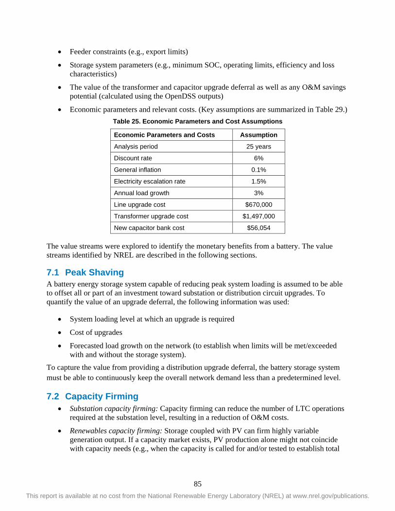
85 This report is available at no cost from the National Renewable Energy Laboratory (NREL) at www.nrel.gov/publications.
• Feeder constraints (e.g., export limits)
• Storage system parameters (e.g., minimum SOC, operating limits, efficiency and loss characteristics)
• The value of the transformer and capacitor upgrade deferral as well as any O&M savings potential (calculated using the OpenDSS outputs)
• Economic parameters and relevant costs. (Key assumptions are summarized in Table 29.) Table 25. Economic Parameters and Cost Assumptions
Economic Parameters and Costs Assumption
Analysis period 25 years
Discount rate 6%
General inflation 0.1%
Electricity escalation rate 1.5%
Annual load growth 3%
Line upgrade cost $670,000
Transformer upgrade cost $1,497,000
New capacitor bank cost $56,054
The value streams were explored to identify the monetary benefits from a battery. The value streams identified by NREL are described in the following sections.
7.1 Peak Shaving A battery energy storage system capable of reducing peak system loading is assumed to be able to offset all or part of an investment toward substation or distribution circuit upgrades. To quantify the value of an upgrade deferral, the following information was used:
• System loading level at which an upgrade is required
• Cost of upgrades
• Forecasted load growth on the network (to establish when limits will be met/exceeded with and without the storage system).
To capture the value from providing a distribution upgrade deferral, the battery storage system must be able to continuously keep the overall network demand less than a predetermined level.
7.2 Capacity Firming • Substation capacity firming: Capacity firming can reduce the number of LTC operations
required at the substation level, resulting in a reduction of O&M costs.
• Renewables capacity firming: Storage coupled with PV can firm highly variable generation output. If a capacity market exists, PV production alone might not coincide with capacity needs (e.g., when the capacity is called for and/or tested to establish total

86 This report is available at no cost from the National Renewable Energy Laboratory (NREL) at www.nrel.gov/publications.
available capacity). A battery system can be used to firm PV output during critical hours, increasing the total capacity payment that a stand-alone PV system can achieve.
7.3 Voltage Support The high variability introduced by distributed PV increases the need for flexible reactive power support. Additional capacitor banks are required to regulate system voltages. Currently, utilities maintain voltages within specified limits using tap changing regulators at the distribution substation and by switching capacitors to follow changes in load. This is especially important on long, radial feeders where a large load such as an arc welder or a residential PV system might cause unacceptable voltage excursions for neighboring customers. An energy storage system can effectively dampen these voltage fluctuations by discharging small amounts of active power.
There is currently no financial compensation for reactive power services in distribution networks. One way to account for the increasing demand for flexible reactive power support in distribution systems is to replicate the lost opportunity cost model currently used with spinning generation at the transmission level.
7.4 Energy Arbitrage Energy storage is charged during off-peak hours and discharged during peak hours to take advantage of the price difference of electricity across time periods. The revenue obtained is the price differential between buying and selling electrical energy minus the cost of losses during the full charge/discharge cycle.
Although market participation is not the focus of the current phase of the project, the value of energy arbitrage is modeled to fully capture the economic impacts of battery operation to provide other distribution system services.
7.5 Multiuse A storage system used for upgrade deferral can simultaneously provide voltage support and capacity firming. Value streams might be stacked, with multiple services provided through a single asset. The added value provided by this flexibility could be quantified and assigned to the battery system as an additional benefit.
7.6 Current System Under Consideration A portion of the TEST FEEDER feeder between the VRFB and the primary overhead line connecting to the substation is capacity constrained (Figure 28). This 1.5-mile #6 overhead cable has a maximum rating of 2.25 MVA, and it directly impacts the maximum charging capacity of the VRFB system. Because the VRFB system is installed downstream of the capacity-constrained line, the total load from that point of the feeder and lower along with battery charging power cannot exceed 2.25 MVA. For example, if the load below the capacity-constrained line is measured at 500 kW, then the battery must charge at or less than 1.75 MW (less than its 2-MW total inverter rating).This constraint was considered in the modeling approach. Loads less than the capacity-constrained line are continuously monitored to ensure that battery charging in optimized dispatches never exceeds line limits unless a line upgrade cost is paid. Optimizations are solved with the option to respect charging constraints based on feeder load at each time step or pay the upgrade cost and avoid all charging limitations.

87 This report is available at no cost from the National Renewable Energy Laboratory (NREL) at www.nrel.gov/publications.
7.7 Value Streams Monetization Results The value streams analyzed along with the main optimal dispatch results are shown in. The report described how these values were derived and other details of the analysis in Table 26.
Table 26. Summary of the Value Streams Analyzed Along with Key Optimal Dispatch Results
Value Stream Monetization Mechanism Year 1 Savings Life-Cycle Savings
Peak shaving Transformer upgrade deferral – $121,135
Capacity firming O&M savings from reduced LTC operations – –
Voltage support New capacitor bank deferral – $7,463
Energy arbitrage Time-shifting energy purchases on the LMP market $56,069 $837,115
Total $965,713
7.8 Field-Testing the Battery At the request of the battery manufacturer, we assisted in operational testing of the VRFB system for a one-week period in April 2018. The peak-shaving/base-loading strategy was executed from April 2–4, the cost-optimal arbitrage strategy was executed from April 4–5, and the hybrid strategy was executed from April 5–6. This testing included three different approaches to dispatching the battery:
1. Heuristic peak shaving/base-loading: This strategy selects set points that the VRFB attempts to maintain for multiple hours. One set point is selected for peak shaving (battery discharging) and is applied during high-load periods of day, and a second set point is selected for base-loading (battery charging) during low-load periods. This strategy requires a load forecast to identify the set points and associated periods of the day in which to implement them. A heuristic method was also used to attempt to align the set points with high/low LMP hours.
2. Cost-optimal arbitrage: This strategy selects multiple set points throughout the day, with a goal of optimizing the revenue that the battery can achieve from the day-ahead LMP market. A total of eight distinct power set points—and associated start times—can be input to the PCS during a given period. This strategy uses the REopt optimization model to select the eight (or fewer) optimal set points to maximize revenue from the day-ahead LMP markets. No load forecast is required for this strategy.
3. Hybrid peak shaving and optimal arbitrage: This strategy uses the same PCS control strategy as the cost-optimal arbitrage (max of eight power set points), and it optimizes revenue from the LMP market while ensuring that the load on the feeder does not exceed

88 This report is available at no cost from the National Renewable Energy Laboratory (NREL) at www.nrel.gov/publications.
a prescribed power limit. This strategy uses the REopt model to select the set points, and it uses a load forecast to inform the peak-shaving objective.
To achieve the load prediction, we trained an ANN to predict the feeder load as a function of meteorological forecasts. The meteorological forecasts, and the subsequent feeder load forecasts, extended through an 18-hour-ahead time horizon at an hourly resolution. The true feeder load and the operating state variables of the VRFB were continuously monitored during the week of testing to enable comparisons with the expected feeder load obtained from the load forecasts and the resultant operational plan.

89 This report is available at no cost from the National Renewable Energy Laboratory (NREL) at www.nrel.gov/publications.
References Cutler, Dylan, Dan Olis, Emma Elgqvist, Xiangkun Li, Nick Laws, Nick DiOrio, Andy Walker, and Kate Anderson. 2017. REopt: A Platform for Energy System Integration and Optimization (NREL/TP-7A40-70022). Golden, CO: National Renewable Energy Laboratory. https://www.nrel.gov/docs/fy17osti/70022.pdf.
Eller, A., and D. Gauntlett. 2017. Energy Storage Trends and Opportunities in Emerging Markets. Washington, D.C.: Energy Sector Management Assistance Program and International Finance Corporation/World Bank.
Eyer, J., and G. Corey. 2010. Energy Storage for the Electricity Grid: Benefits and Market Potential Assessment Guide. Albuquerque, NM: Sandia National Laboratories.
Jenkins, John D. 2014. “Capital Workpapers to Prepared Direct Testimony of John D. Jenkins on Behalf of San Diego Gas & Electric Company.” November 2014. https://www.sdge.com/sites/default/files/SDGE-09-CWP_EDIST.pdf.