Valuing the Clean Air Act:

How Do We Know How Much Clean Air is Worth?

J. Scott Holladay

Discussion Paper No. 2011/1

Valuing the Clean Air Act: How Do We Know How Much Clean Air is Worth?

In March, the Environmental Protection Agency (“EPA”) released the Second Prospective Study of the impact of the Clean Air Act. This study, entitled The Costs and Benefits of the Clean Air Act from 1990-2020, detailed an exhaustive effort to calculate the impact of the Clean Air Act on human health, the economy and the environment. The study analyzed new regulations associated with the Clean Air Act Amendments passed by Congress in 1990. Specifically the study focuses on how polluters respond to the rules, how much these responses reduce pollution, and how those reductions in pollution affect ecological systems and human health.

The analysis finds that the Clean Air Act regulations will reduce in air pollution and create sizeable health benefits. The annual costs of the regulations analyzed in the study increase from $20 billion in the year 2000 to $65 billion by 2020. These costs are swamped by the projected benefits of the reduction in air pollution, starting at $770 billion in 2000 and rising to $12 trillion by 2020. The study projected the benefits of the Act would exceed the costs by a factor of 30 over the study period.

This paper:

• Summarizes the process of tabulating the costs and benefits of the Clean Air Act and forecasting its impacts into the future.

• Finds that benefits primarily take the form of reduced mortality associated with reduced exposure to air pollution.

• Outlines the process for translating reductions in mortality to dollars using the Value of a Statistical Life.

• Highlights the process of monetizing benefits—translating changes in human health and welfare into dollars and cents—to facilitate comparison to cost estimates.

• Describes the benefits of reduced air pollution that EPA identified, but could not value.

1

Evaluating the Clean Air Act

Section 812 of the 1990 Clean Air Act Amendments requires EPA to periodically report on the impact of the Clean Air Act (CAA) on “public health, economy, and environment of the United States.” Congress goes on to require that the effects of the CAA on public health, economic growth, employment, and productivity be analyzed, and that the results be reported to Congress. EPA has fulfilled this statutory requirement by publishing detailed cost-benefit analyses of various regulations promulgated under the CAA, and by making the results available to Congress and the general public.

In 1997 EPA released the first retrospective study estimating the cost and benefits of the 1970 CAA, over the period of 1970 to 1990. The study focused on the impact of the CAA on six specific pollutants for which data was readily available.1

In 2011 EPA released another report (the Prospective Study) projecting the costs and benefits associated with the 1990 amendments to the CAA between 1990 and 2020. The primary goal of this study is to “estimate the direct costs and direct benefits of the Clean Air Act as a whole, including major federal, state, and local programs implemented to meet its requirements.”

The results suggested that the benefits of the CAA regulations exceeded the cost by at least 10-to-1, and by as much as 100-to-1. In 1999 a follow-up analysis projecting costs and benefits from 1990-2010 was released. This report calculated that the additional benefits of the 1990 Clean Air Act Amendments during this period would outweigh the additional costs by four-to-one.

2

The new regulations strengthened existing environmental rules generating further benefits and costs above and beyond those associated with the original CAA. For that reason EPA decided to evaluate the costs and benefits of the CAAA separately from the rest of the program. The Prospective Study does not estimate the impact of regulations associated with the CAA, but estimates of the additional impact of the regulations created under the CAAA taking the structure of the original CAA as given.

The Clean Air Act Amendments (CAAA) introduced new programs to reduce emissions associated with acid rain and ozone depletion, but for the most part they simply modified the existing Clean Air Act by increasing the stringency of existing air pollution standards.

Though the Clean Air Act Amendments included provisions on everything from gasoline fuel blends to the management of continental shelf resources, EPA chose to focus its analysis on the “major emissions regulatory programs.”3

These regulations included provisions requiring polluters to install abatement technology for Volatile Organic Compounds (VOCs) and nitrous oxides (NOx) in areas with high levels of pollution; control technology on engines for vehicles; emissions standards for hazardous air pollutants; and programs to reduce emissions associated with acid rain from electricity generators.

The Methodology of the Retrospective Study

Estimating and quantifying the costs and benefits of a major regulatory program like the Clean Air Act Amendments requires a variety of engineering, economic, and health modeling tools which are frequently used in environmental economic analysis by EPA and other analysts. EPA’s decision to limit the analysis to direct costs

1 The study focused on the “criteria” pollutants that the EPA is required to regulate based on specific human health criteria rather than cost. This ignores potential benefits from other types of air pollutants that are frequently emitted in conjunction with the criteria pollutants. 2 U.S. Environmental Protection Agency Office of Air and Radiation. 2011. The Benefits and Costs of the Clean Air Act from 1990 to 2020: Summary Report. p6. 3 U.S. Environmental Protection Agency Office of Air and Radiation. 2011. The Benefits and Costs of the Clean Air Act from 1990 to 2020: Final Report – Revision A. p1-5.

2

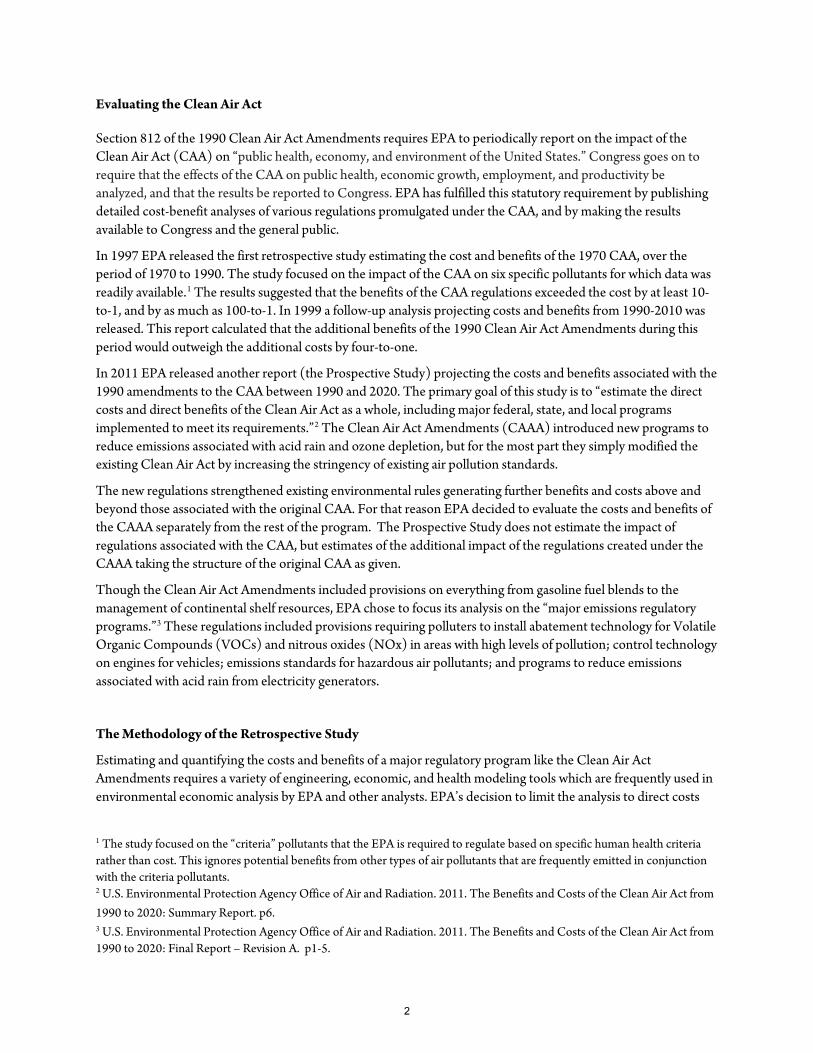
and benefits of the CAAA simplifies the analysis considerably. Researchers must estimate the impact of reduced air pollution on children’s health (a direct effect), but they need not estimate how improvements in children’s health affect parents’ productivity (an indirect effect). While these indirect costs and benefits may be large, they are very difficult to calculate. Attempting to estimate the indirect costs and benefits would inject a huge amount of uncertainty into the analysis and potentially dilute the reliability of the direct effect results.

Figure 1: Analytic Sequence Flow Chart (Source: Based on EPA Second Prospective Study Figure 1-2)

The first step in any cost-benefit analysis is to define the scenarios to be modeled and compared. Economists rely on the “with-without” principle to create statistical evaluations of policy.4 In the Prospective Study the researchers estimate the level of emissions with the CAAA regulations in place, called the “with” scenario. To estimate future pollution emissions under CAAA regulations EPA follows the standard practice of taking the current rate of emissions and scaling it up by forecasted economic growth.5

Defining the “without” scenario requires estimating the level of pollution emissions in the absence of the CAAA regulations. Of course the researchers cannot observe this hypothetical emissions level, so they are forced to

4 Field, B. and M. Field. Environmental Economics: An Introduction Third Edition. Boston, MA: McGraw Hill Irwin. p161. 5 This is one way in which the Prospective Study differs from typical cost-benefit analyses. Most CBA’s are projecting the cost and benefits of regulations that have not yet entered into force and therefore cannot be projected from current emissions levels. In these cases, the with (projecting from existing trend) and without (projecting hypothetical alternative) scenarios are reversed.

Scenario Development

Sector Modeling

Emissions

Air Quality Modeling

Health Human Welfare

Economic Valuation

Benefit-Cost Comparison

Direct Costs

3

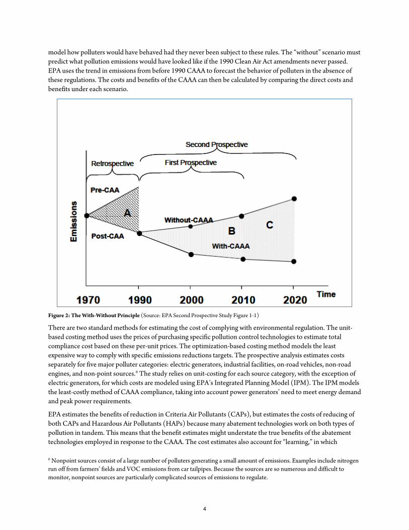
model how polluters would have behaved had they never been subject to these rules. The “without” scenario must predict what pollution emissions would have looked like if the 1990 Clean Air Act amendments never passed. EPA uses the trend in emissions from before 1990 CAAA to forecast the behavior of polluters in the absence of these regulations. The costs and benefits of the CAAA can then be calculated by comparing the direct costs and benefits under each scenario.

Figure 2: The With-Without Principle (Source: EPA Second Prospective Study Figure 1-1)

There are two standard methods for estimating the cost of complying with environmental regulation. The unit-based costing method uses the prices of purchasing specific pollution control technologies to estimate total compliance cost based on these per-unit prices. The optimization-based costing method models the least expensive way to comply with specific emissions reductions targets. The prospective analysis estimates costs separately for five major polluter categories: electric generators, industrial facilities, on-road vehicles, non-road engines, and non-point sources.6

EPA estimates the benefits of reduction in Criteria Air Pollutants (CAPs), but estimates the costs of reducing of both CAPs and Hazardous Air Pollutants (HAPs) because many abatement technologies work on both types of pollution in tandem. This means that the benefit estimates might understate the true benefits of the abatement technologies employed in response to the CAAA. The cost estimates also account for “learning,” in which

The study relies on unit-costing for each source category, with the exception of electric generators, for which costs are modeled using EPA’s Integrated Planning Model (IPM). The IPM models the least-costly method of CAAA compliance, taking into account power generators’ need to meet energy demand and peak power requirements.

6 Nonpoint sources consist of a large number of polluters generating a small amount of emissions. Examples include nitrogen run off from farmers’ fields and VOC emissions from car tailpipes. Because the sources are so numerous and difficult to monitor, nonpoint sources are particularly complicated sources of emissions to regulate.

4

polluters develop new technology and techniques for reducing emissions at low costs. The default learning rate used is 10%, meaning that, all else being equal, the costs of meeting the standards should fall around 10% per year. This assumption is consistent with the latest economic research on the subject.7

The Prospective Study presents annual cost estimates for 1990, 2000 and 2010 for each source category, and for many of the specific regulations associated with the CAAA. The results vary across time due to economic growth, different levels of learning across industries and pollution control regulations. The total estimated costs range from $19.9 billion in 1990 to $65.5 billion by 2010. Regulations of on-road vehicles account for nearly half of the estimated costs, and those for electric power generators make up more than 15% of estimated total costs.

Estimating the benefits of the CAAA is significantly more difficult and requires several intermediate steps. First, the study estimates pollution emissions in both the “with CAAA regulation” and “without CAAA regulation” scenarios to determine how the CAAA has affected the flow of pollution into the atmosphere. To create the “without” scenario, EPA makes use of the National Emissions Inventory, which catalogued emissions of Criteria Air Pollutants prior to the implementation of the CAAA. Applying that data to estimates of economic and population growth, EPA is able to project what emissions would have looked like had the CAAA not been implemented. Defining the “with” scenario requires mapping individual provisions of the CAAA to the source category that is impacted, and then projecting the effect on emissions using the appropriate model for that source category. For example, the CAAA included standards for pollution emissions by cars and light trucks, called “Tier 1 emissions standards,” that reduced on-road emissions significantly. Using the estimates from EPA’s MOBILE model of vehicle miles traveled, the study’s authors can estimate total emissions from vehicles that comply with the new regulations. This process is repeated for each CAAA regulation and emissions source until all future emissions pathways have been evaluated. EPA completes the “with” scenario by summing emissions across all source categories.

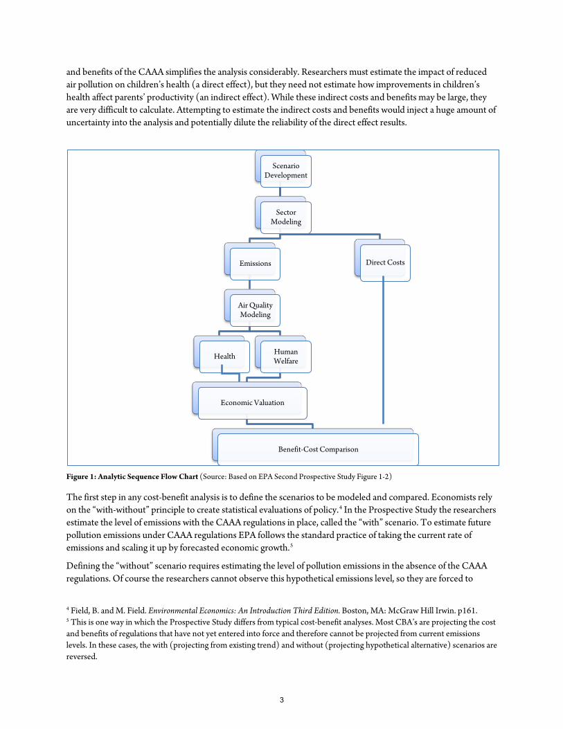
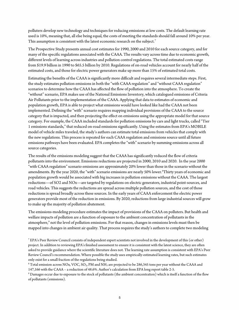
The results of the emissions modeling suggest that the CAAA has significantly reduced the flow of criteria pollutants into the environment. Emissions reductions are projected in 2000, 2010 and 2020. In the year 2000 “with CAAA regulation” scenario emissions are approximately 20% lower than those in the scenario without the amendments. By the year 2020, the “with” scenario emissions are nearly 50% lower.8

The emissions-modeling procedure estimates the impact of provisions of the CAAA on polluters. But health and welfare impacts of pollution are a function of exposure to the ambient concentration of pollutants in the atmosphere,

Thirty years of economic and population growth would be associated with big increases in pollution emissions without the CAAA. The largest reductions—of SO2 and NOx—are targeted by regulations on electric generators, industrial point-sources, and road vehicles. This suggests the reductions are spread across multiple pollution sources, and the cost of those reductions is spread broadly across these sources. In the early years of CAAA enforcement the electric power generators provide most of the reduction in emissions. By 2020, reductions from large industrial sources will grow to make up the majority of pollution abatement.

9

7 EPA’s Peer Review Council consists of independent expert scientists not involved in the development of this (or other) project. In addition to reviewing EPA’s finished assessment to ensure it is consistent with the latest science, they are often asked to provide guidance where the scientific literature does not. The learning rate assumption is consistent with EPA’s Peer Review Council’s recommendation. Where possible the study uses empirically-estimated learning rates, but such estimates only exist for a small fraction of the regulations being studied.

not the level of pollution emissions. For that reason, changes in emissions levels must then be mapped into changes in ambient air quality. That process requires the study’s authors to complete two modeling

8 Total emission across NOx, VOC, SO2, PM and NH3 are projected to be 286,345 tons per year without the CAAA and 147,166 with the CAAA – a reduction of 48.6%. Author’s calculation from EPA long report table 2-5. 9 Damages occur due to exposure to the stock of pollutants (the ambient concentration) which is itself a function of the flow of pollutants (emissions).

5

challenges: model the movement of pollution through the atmosphere, and model the chemical changes that occur when pollutants interact with air, sunlight, and each other. The Community Multi Scale Air Quality (CMAQ) model described in Byun and Ching (1999) is the most advanced tool for projecting “atmospheric processes affecting transport, transformation, and deposition of such pollutants as ozone, particulate matter, airborne toxics, and [acid rain precursors].” 10

Emissions levels estimated in the previous step are fed into the model. In order to generate accurate assessments of ambient pollution concentrations over space and time, emissions levels must be calculated hourly at a small scale. The CMAQ requires emissions calculated in a grid of cells ranging from 12-36 square kilometers. The model also requires hourly meteorological data (temperature, wind speed and precipitation among others) at a similar resolution. The model produces estimated ambient pollution concentrations which are then calibrated against actual pollution monitor data, and corrected to ensure accuracy.

Figure 3: Annual Emissions With/Without the CAAA in 2020 (Source: EPA Second Prospective Study Table 2-5)

The calibrated CMAQ produces projections of ambient pollution concentrations for both scenarios. The projections are calculated at the same small-scale resolution, generating tens of thousands of estimates that span the country. Comparing pollution concentrations between scenarios suggests that the CAAA is associated with significant reductions in ambient pollution concentration, the magnitude of which vary geographically. The largest reductions are concentrated in California’s Imperial Valley, Southern California and the Great Lakes region. Reductions of over 50% are observed in numerous cells, with Chicago experiencing reduction of over 70%

10 Byun, D.W. and Ching, J.K.S., eds. 1999. Science Algorithms of the EPA Models-3 Community Multiscale Air Quality (CMAQ) Modeling System. U.S. Environmental Protection Agency, Office of Research and Development. EPA/600/R-99/030. p 1-3.

0

50

100

150

200

250

VOC NOx CO SO2 PM10 PM2.5 NH3

Without CAAA

With CAAA

6

in PM2.511 concentrations and Los Angeles seeing a reduction of more than 50% by 2020. Ozone reductions are

somewhat smaller as a fraction of total ambient concentration, but still significant. Benefits are geographically distributed much more evenly than for PM, but many urban areas experience little or no reduction in ozone concentrations.12

After using the MAQS to predict local air quality in each scenario, the results can be mapped onto human health and welfare impacts. The small scale of ambient pollution data (12 to 36-square km cells) allows the study’s authors to map changes in pollution exposure onto detailed population data. EPA employs a specially built epidemiological model, the Environmental Benefits Mapping and Analysis Program (known as BenMAP), to predict changes in human health and welfare from changes in the concentration and mixture of air pollutants. BenMAP requires three inputs: 1) annual levels of ambient pollution concentration, 2) functions that map changes in pollution exposure to human health effects, and 3) a monetization function that assigns dollar values to health outcomes. The output of the model is an estimate of the change in the number of pollution related mortalities, along with additional welfare measures such as days of work missed and trips to the emergency room. The model also provides monetary values associated with each of those changes in health and welfare.

The results from BenMAP suggest that the CAAA is associated with significant improvements in human health and welfare. In 2020, the “with CAAA regulation” scenario has an estimated 230,000 fewer deaths associated with exposure to PM and ozone than the alternative scenario. Nonfatal heart attacks are projected to drop by 200,000, 17 million fewer days of work will be missed, and emergency room visits related to asthma are projected to drop by 120,000 thanks to reduced exposure to pollutants.

Predicting ecological and natural resources impacts of the CAAA is somewhat more difficult. No unified model exists to map changes in ambient pollution concentration to changes in resource productivity, recreation choices, and ecological system functioning; all of which are impacted by exposure to pollutants. This forces the authors to calculate these impacts on a case-by-case basis. The report seeks to classify four different types of non-human benefits associated with the pollution reductions caused by the CAAA: enhanced forest and agricultural plant growth, enhanced visibility in recreational and residential, reduced damage to certain building and structural materials, and acidification of freshwater bodies. Each class of benefit must be estimated using separate models informed by the academic literature in that particular area, and then the benefit must be monetized based on the results of a different category of literature. This process is significantly more difficult than valuing the human health and welfare benefits of reduced pollution.

These disparate classes of benefits of improved air quality are calculated in a one-off manner. For example, the impact of nitrogen and sulfur disposition on lake acidity is estimated from a case study from New York’s Adirondack’s region using the Model of Acidification of Groundwater in Catchments (MAGIC). This model describes how acid is transported through rain and snowmelt into the groundwater and ecosystems of the region. These results are then used in two ways: 1) to estimate the growth rate of forests exposed to different levels of acidity, and 2) to estimate the level of lake acidity and its impact on recreational fishing. The study’s authors implement similar ad-hoc modeling efforts for each of the other categories of ecological and natural resource benefits to produce estimates suitable for quantification in the next step of the analysis.

11 PM2.5 is particulate matter with a diameter of 2.5 microns or less. These fine particles are small enough to be inhaled directly into the lungs and pass into the blood stream. Particulate matter is associated with a host of pulmonary and cardiac illnesses 12 The report cites a complex chemical process known as “NOx-scavenging,” in which nitrogen oxide pollution can actually serve to reduce ozone concentrations, as the likely cause. Because the CAAA is reducing NOx levels it may in a few cases have the counterintuitive impact of actually increasing ozone levels in some areas. This caveat aside, the overall result of the CAAA is a marked decrease in regional ozone concentrations.

7

Valuing the Benefits

This section focuses on the difficult process of monetizing the projected impacts of improvements in air quality. EPA relies on a series of specially designed models to map reductions in emissions to improvements in air quality, and improvements in air quality to enhancements in mortality, health, welfare and ecological benefits. The process of translating these varied benefits into dollars and cents requires EPA to match each category of benefit with the appropriate value using existing studies. The Second Prospective Study does no new field work to estimate previously unknown values, but does highlight several places where such work could improve the quality of its monetized estimates. Monetization is used to measure premature deaths (mortality) and additional incidence of disease (morbidity) avoided due to reduced exposure to pollutants, and translates those outcomes into a common denominator to facilitate comparison with the costs of a regulation.

Monetizing benefits is a necessary step in evaluating the impact of the CAAA. Section 812 of the CAAA has been interpreted to mean that EPA is required to report to Congress on the economic costs and benefits of the CAAA as well as the impact of the Act on human health and welfare.13

This willingness-to-pay (WTP) of individuals for reductions in risk varies by the type of risk. Consumers frequently exhibit a higher WTP to reduce the risk of transportation accidents than exposure to natural hazards, for example.

Providing measures of economic benefits without quantifying and monetizing the human health and welfare benefits would provide a misleading impression of the effectiveness of the Act, particularly when compared to the dollar value of costs. Monetizing benefits also allows EPA to compare different regulations associated with the Act to determine which types of rules are most effective in generating benefits. There is no objective basis for determine whether a rule that leads to a reduction in lost works days is more effective than one which reduces incidence of lower respiratory symptoms. Monetization, done properly, helps EPA assess those tradeoffs.

14

The process of monetization can be controversial. Some observers argue that quantifying the benefits of reduced pollution, such as health or even risk of dying, monetization cheapens priceless things.

For that reason each of the different types of risk that the CAAA reduces must be valued separately. EPA has considerable experience collecting academic studies of risk valuation and applying these findings to forecasted risk-reductions from models like BenMAP. While no general model for monetizing benefits exists, there is significant economic literature to which study authors can turn. Dozens of valuation studies have been conducted by economists and published in reputable economic journals after undergoing a peer review process. These studies tend to value one class of benefit at a time.

15

Reduced Mortality

These arguments represent a fundamental misunderstanding of the monetization process. The goal of monetizing benefits is not to measure the value of human health and wellbeing, but to measure the value of risk, something that every individual does on a regular basis. When choosing whether to purchase a car with side-impact airbags, to wear a helmet on a short bike ride, or to purchase more expensive organic produce, consumers are making an implicit choice between price and risk. The monetization process seeks to measure that tradeoff and determine how much consumers are willing to pay for reductions in risk.

The Second Prospective Study’s analysis suggests that the CAAA will be associated with avoiding 230,000 pollution related deaths in 2020. Improvement in human health represents the highest valued benefit of the

13 U.S. Environmental Protection Agency. 1990. The Benefits and Costs of the Clean Air Act, 1970 to 1990. p1. 14 G. W. Fischer et al. 1991. “What Risks Are People Concerned About?” Risk Analysis 11, 303-314. 15 Ackerman, Frank and Lisa Heinzerling. 2002. Pricing the Priceless: Cost- Benefit Analysis of Environmental Protection, 1 50 U Pa L Rev 1553, 1570-73.

8

CAAA measured by this study. This reduction in mortality is evaluated as a decrease in the chance of dying due to exposure to pollution. This reduction in mortality risk is spread across everyone exposed to pollution rather than concentrated in specific individuals whose death was averted.

The benefits of this reduction in mortality are evaluated using a concept known as the Value of a Statistical Life (VSL). The VSL is a measure of people’s willingness to pay for small reductions in risk of mortality. This willingness-to-pay is typically measured as the amount a person would pay to reduce the risk of dying in a particular activity by one-one millionth.16 This individual willingness-to-pay for a small reduction in individual risk of death is then summed for convenience and discussed in units of one fatality. This is what is meant by saying the VSL does not provide an estimate for the value of a life,17 but of a “statistical life,” which is just value of risk reduction. The amount an individual is willing to pay, multiplied by one million provides an estimate for how much an entire group (in this case, the population of the U.S.) would be willing to pay for the reduction in a small risk of dying. 18

Again, it is important to note that the VSL does not value any individual’s life or value how much a respondent is willing to pay to save any single person’s life. The VSL is only an appropriate tool to measure WTP for small reductions in risk of mortality. For that reason it is an appropriate tool to use when valuing lives saved by environmental regulation. BenMAP’s results suggest that the CAAA will reduce mortality by 230,000, but it does not tell us which 230,000 people will live longer thanks to reduced exposure to pollution. When compared to the population of the United States

This value is the VSL. For example if an environmental regulation reduced the risk of fatality by one-one millionth for each person in the U.S. it would save around 300 statistical lives. A firefighter who pulls someone out of a building does not save a statistical life, but does save an actual life. That action cannot be valued using the VSL.

19

Economists have made numerous efforts to calculate the VSL over the last thirty years. Consumers make tradeoffs between risk and price in market contexts all the time, but isolating willingness-to-pay for mortality risk reductions from these market transactions can be difficult. For example, cars with side-impact air bags available as optional equipment tend to be different in systematic ways from those that provide air bags standard. The cars with standard side airbags might also tend to have power seats, heated mirrors and other expensive options. If that is the case using the price of side-impact airbags as a standalone option is a poor proxy for the full willingness-to-pay for this reduction in risk. For these reasons calculating the VSL from consumer decisions is empirically difficult.

any individual’s chances of living longer are fairly small. That is precisely the type of risk that the VSL is designed to value.

There are two primary empirical techniques employed in the estimation of the VSL. The first is known as contingent valuation, in which survey respondents are asked a series of hypothetical question in an effort to assess their willingness to pay for reductions in mortality risk. Participants are typically informed about how their decision (purchasing a car with side impact air bags, for example) would affect their probability of mortality. They are then offered a series of decisions (cars with varying options packages and prices) designed to precisely identify their WTP to reduce their risk of dying in an auto accident. While contingent valuation studies allow the

16 The WTP to reduce risk is measure as $/micro-mort/person, where a micro-mort is a one in one million chance of dying. For the purposes of VSL, this micro-mort unit is converted to a unit of a single life, for ease of reference. But the underlying value is still a reflection of WTP regarding a micro-mort. 17 Obviously the willingness to pay to reduce the risk of certain death is all of an individual’s money. This is why the VSL can only be used to estimate WTP for small reductions in mortality risk. 18 Newbold, Stephen C. 2011. “Valuing Health Risk Changes Using a Life-cycle Consumption Framework.” Paper presented at the Valuing Lives: A Conference on Ethics in Health and the Environment, New York, NY. 19 The projected U.S. population in 2020 is 342 million. See Census Bureau’s 2008 National Population Projections (http://www.census.gov/population/www/projections/2008projections.html).

9

researcher to ask questions designed to isolate the WTP for reductions in mortality, they have been criticized for relying on hypothetical questions rather than actual market data.

The other primary technique used in estimating the VSL relies on labor market studies. Jobs have different probabilities of workplace mortality, and industries that have higher levels of worker mortality tend to pay more to compensate workers for the added risk. Comparing the wage differential in two very similar jobs with different probabilities of work place mortality allows researchers to assess how much workers must be paid to accept an increase in the chance of dying. Wage differentials across industries, in conjunction with the differences in the probability of workplace fatality, allow the researchers to estimate the VSL. Labor market studies rely on market data, having the advantage of capturing actual behavior, but they require identifying all the differences between jobs that might impact wage differentials. There is a wealth of survey and statistical data describing these jobs and industries, but any omitted difference between jobs that affects wages could bias the estimate of the VSL.

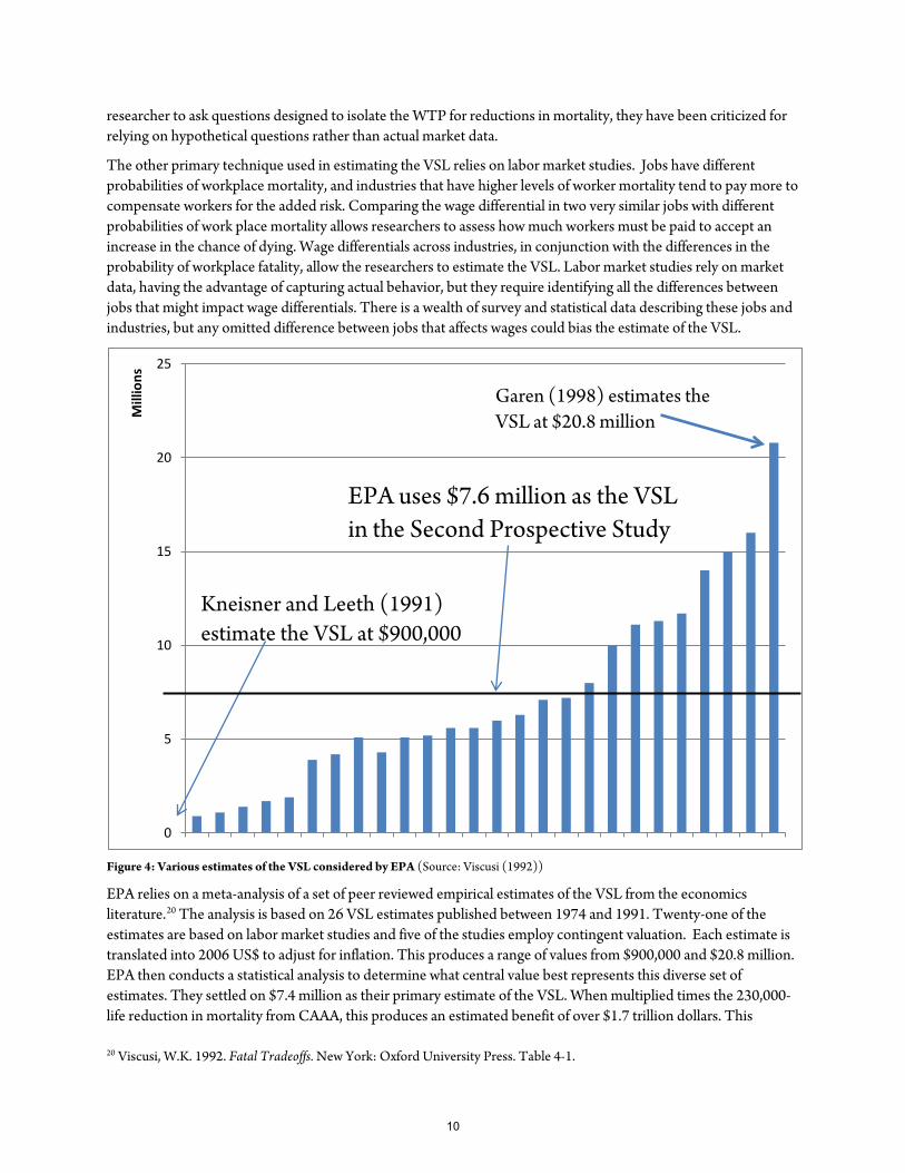
Figure 4: Various estimates of the VSL considered by EPA (Source: Viscusi (1992))

EPA relies on a meta-analysis of a set of peer reviewed empirical estimates of the VSL from the economics literature.20

20 Viscusi, W.K. 1992. Fatal Tradeoffs. New York: Oxford University Press. Table 4-1.

The analysis is based on 26 VSL estimates published between 1974 and 1991. Twenty-one of the estimates are based on labor market studies and five of the studies employ contingent valuation. Each estimate is translated into 2006 US$ to adjust for inflation. This produces a range of values from $900,000 and $20.8 million. EPA then conducts a statistical analysis to determine what central value best represents this diverse set of estimates. They settled on $7.4 million as their primary estimate of the VSL. When multiplied times the 230,000-life reduction in mortality from CAAA, this produces an estimated benefit of over $1.7 trillion dollars. This

0

5

10

15

20

25

Mill

ions

Garen (1998) estimates the VSL at $20.8 million

Kneisner and Leeth (1991) estimate the VSL at $900,000

EPA uses $7.6 million as the VSL in the Second Prospective Study

10

represents the largest single benefit valued in the Study and accounts for eight-five percent of the total projected benefits in 2020.

Improved Human Health and Welfare

Similar to the valuation of human mortality, valuing human morbidity requires matching health outcomes to valuations on a case-by-case basis. There are two major sources of monetizations for human health and welfare impacts of the CAAA: 1) market data and 2) contingent valuation surveys. EPA identifies health impacts as predicted by the BenMAP model and then searches the existing literature for monetized valuations of those health effects. If enough studies have been conducted, EPA can generate a distribution of monetization estimates using range of values calculated in previous work as they did with the VSL estimates described above. Different physical ailments and poor health outcomes have different values, and for many of these health effects, there are very few published monetization studies. As opposed to more thoroughly studied phenomena in which a distribution of possible values are available, the EPA in these cases must use a single estimate, and the uncertainty surrounding that estimate is difficult to quantify. Health endpoints that have not been monetized in peer-reviewed studies are not included in the benefit numbers described in this study, and are categorized as “unquantified benefits.”21

There have been several studies of individuals’ willingness to pay to avoid chronic bronchitis and associated symptoms. This work can be used to generate a distribution of the benefits associated with the 75,000-case reduction in incidence of chronic bronchitis in 2020 projected by this study. A willingness-to-pay survey asked respondents a series of questions to assess their willingness to trade off different risks (risk of car accident versus bronchitis) and their willingness to trade off risks for money.

22 The results suggest that respondents would pay approximately $457,000 to avoid chronic bronchitis. A second paper, testing the impact of information on respondents’ willingness-to-pay to reduce risk, found that willingness-to-pay to avoid bronchitis varied over the survey group in a manner predictably related to income.23

In some cases EPA is able to take advantage of direct measures of the costs of health care to monetize the benefits of reduced exposure to air pollution. When valuing nonfatal heart attacks, EPA includes two types of heart attack costs—the direct medical costs of treatment, and the value of lost earning opportunities. The value of lost earnings, as estimated by Cropper and Krupnick in terms of a five-year period of lost earnings, varies with age. For patients who have a heart attack between the ages of 25-45 the lost wages are estimated to be $9,631 and for those

This information on how WTP varies with income and severity of bronchitis symptoms was used to generate a distribution of the possible monetized benefits of avoiding bronchitis. Taking the results of these studies together, EPA chose a value of $490,000 per bronchitis case avoided in 2020.

21 Costs are significantly easier to monetize than benefits meaning that unquantified benefits bias cost-benefit analysis against finding a regulation is justified, but also ensure that the results are conservative and defensible. The more important unquantified benefits are to a particular regulation the more important tools besides cost-benefit analysis becomes in evaluating the policy options. 22 Viscusi, W.K., W.A. Magat, and J. Huber. 1991. “Pricing Environmental Health Risks: Survey Assessments of Risk-Risk and Risk-Dollar Trade-Offs for Chronic Bronchitis” Journal of Environmental Economics and Management, 21: 32-51. 23 Specifically, as income rises, willingness-to-pay increases with an elasticity of 0.18. (An increase in income of 1% increases WTP by 0.18%). See Krupnick, A.J. and M.L. Cropper. 1992. The effect of information on health risk valuations. Journal of Risk and Uncertainty 5(1): 29-48 for additional distributional information.

11

between 45-54 lost wages would be $14,195. Apart from lost wages, two estimates of the direct costs of treating a heart attack are estimated in the literature. Wittels et al. estimated a total cost of $141,124 and Russell et al. estimate around $28,000 after controlling for cost inflation. EPA takes a simple average of these estimates to generate an estimated direct medical cost. Summing the medical costs and lost wages generates a range of estimated benefits from $84,121 for the very young and $166,222 for those in their earnings prime. These values serve as the monetized benefits for each non-fatal heart attack avoided.

The benefits from other improvements in human welfare are somewhat harder to monetize. Valuing lost work and school days requires EPA to use U.S. census data to calculate the amount the average worker earns per day. To do this they take annual median income estimates from the 2000 Census and divide by the number of work days in the year. This produces a monetized value of $149 per lost work day. The value of a lost school day is estimated in a similar manner. The estimate is based on the probability that a parent must stay home to look after the child, and then uses the parents lost income for that day as a proxy for the cost. This generates a value of $89 per lost school day. This approach captures the market value of lost school days, but does not include other costs to missing school such as falling behind in lessons or missing afterschool opportunities. For that reason these estimates serve as a lower bound for the possible benefits to reducing lost work and school days due to exposure to air pollution.

Dozens of other benefits are monetized in a similar manner, using the best available economic estimates.24

Ecological and Natural Resource Effects

The monetized values vary tremendously from $18 to avoid lower respiratory symptoms (shortness of breath, coughing, fatigue) to $490,000 to avoid chronic bronchitis. Each of the monetized benefits is then multiplied by the number of cases avoided due to regulations implemented under the CAAA. This generates a benefit estimate for each health and welfare endpoint, over twenty in all. These benefits are then summed to calculate the total health and welfare benefits of the CAAA. The value of these health and welfare benefits is estimated at $10.4 billion in 2000 and rises to $57.1 billion by 2020. The estimated costs of compliance with the CAAA are $20 billion in 2000 and $65 billion in 2020, suggesting that this single class of benefits nearly outweigh the total compliance costs.

The Second Prospective Study has identified several benefits of the CAAA that do not impact human health and welfare directly, but have economic consequences that can be measured. There are four classes of indirect benefits predicted by EPA’s models that can be monetized: 1) enhanced forest and agricultural plant growth, 2) enhanced visibility in recreational and residential areas, 3) reduced damage to certain building and structural materials and 4) acidification of freshwater bodies and impairment of timber growth. The Study monetizes each impact separately using market data where possible, and relying on survey data for benefits that cannot be valued by observing market transactions directly.

Air pollution retards the growth of all types of plants, but monetizing the impact for noncommercial plants is difficult. For that reason the Study focuses on improved growth in agricultural crops and forests. The results of the

24 The full list includes chronic bronchitis, nonfatal myocardial infarction, hospital admissions for a variety of ailments (COPD, Asthma, Pneumonia, Ischemic Heart Disease, dysrhythmia, congestive heart failure, emergency room visits for asthma) and respiratory ailments not requiring hospitalization (upper respiratory symptoms, lower respiratory symptoms, asthma exacerbations, acute bronchitis, work days lost, minor restricted activity days and school days lost).

12

ecological modeling processes provide estimates of expected improvements in yield for eleven crops and two types of trees. These benefits could be monetized directly using the estimated crop values of the additional production, but that would ignore the way the agricultural sector responds to changing productivity. As the yields go up, farmers will respond by changing their mix of crops and farm land will become more valuable. To capture the full impact of the CAAA, the Study uses the Forest and Agriculture Sector Optimization Model (FASOM), which projects how agriculture will respond to reduced air pollution. The results suggest very small benefits in the forestry sector, but the agricultural sector enjoys benefits of $10.6 billion a year.

There is evidence that individuals are willing to pay for better visibility where they live and at certain recreation destinations. The range of estimated WTP from the literature for a hypothetical ten percent improvement in residential visibility is $14 to $145 based on numerous contingent valuation surveys. EPA separately values the benefits for improved visibility at recreation sites using estimates of WTP for improvements in visibility at national parks along with regional estimates of the CAAA’s impact on air quality. Previous work has found that individuals might be willing to pay more for air quality improvements at certain national land marks, like the Grand Canyon. Together the improved visibility is valued at $67 billion in 2020.

Air pollution causes aesthetic and structural damage to metals, stone, and wood. The Study estimates the value of damaged materials and the maintenance costs associated with reducing pollution-related wear. Acidic deposition related to pollution has an identifiable impact on the rate of decay of sensitive materials. EPA has developed regional inventories of materials that are sensitive to pollution exposure, estimating the value of this reduced rate of decay using market data on the costs of materials and maintenance. The total monetized benefit was $110 million.

The final class of monetized benefits is the reduction in acidification in freshwater bodies. The value of reduced acidification is approximated from two types of benefits: improved recreational fishing and faster forest growth. There are certainly numerous other benefits of reduced acidity in the water table, but only these specific benefits could be monetized. WTP for improved water quality is measured by the number of lakes that become safe for fishing as a result of CAAA regulations. This value is estimated from survey data at approximately $7 per-lake-per-year. The more lakes that experience water quality improvements, the lower the WTP will be for any single lake becoming fishable. Estimated tree growth leads to improved forestry productivity and extra revenue for loggers. Valuing trees based on market data for round logs and wood chips, reduced air pollution could lead to between $1 and $1.5 million annually in additional logging benefits.

Unquantified Benefits

EPA’s retrospective study fails to quantify several types of benefits associated with improved air quality. This is typically due to there being an insufficient number of reliable valuation studies in the economic literature. EPA did no field work to generate valuations for benefits, relying only on monetization estimates from peer-reviewed literature. Many types of benefits have not been monetized by academic economists, due to technical difficulties or lack of information. EPA also excluded from the analysis some titles of the CAAA that made permitting and other administrative tasks more efficient. Any benefits from improving the regulatory process remain unquantified.

13

Many of the human health impacts of reduced exposure to pollution have been quantified, but some specific health impacts or symptoms remain unquantified. Table 5-1 in the Study lists the quantified and unquantified health impacts of PM and Ozone exposure separately. Among the health impacts that are not included in the benefits estimates are: reduction in low birth-weight babies, reduced cancer rates, non-asthma emergency room visits, and a host of others. One unquantified impact, an increase in exposure to UVB rays associated with a reduction in air pollution, may have positive or negative health impacts; all other unquantified impacts are clearly benefits.

Monetizing the ecological benefits of the CAAA is particularly difficult. Even modeling the impact of reductions in ambient pollution levels is difficult. It requires a complex understanding of the interactions between air quality and biological processes across an incredible range of species. Some of the benefits of reduced pollution might be hard to imagine and therefore impossible to quantify. Even modeled impacts of the CAAA might not be entirely quantifiable. The impacts of reduced acidification are felt throughout the ecosystem, but only a small fraction of that benefit is monetized. Any reduction in water treatment costs, improved agricultural productivity related to irrigation or human health benefits are not included in the monetary estimate of the benefits reduced acidification.

Ancillary reductions in hazardous air pollution (HAP) emissions are included in the cost estimates, but not in the benefits estimates. The analysis focuses purely on the benefits of criteria pollutant reductions. It is possible that CAAA regulations are associated with significant reductions in HAPs. A case study in the First Retrospective Study found significant benefits associated with reductions in HAPs, but estimating the human health impacts of the hundreds of hazardous pollutants that are emitted alongside the criteria pollutants is extremely difficult and EPA felt it was beyond the scope of the Prospective Study.

The fact that these benefits cannot be monetized does not make them any less real, or relevant to decision makers. A cost-benefit analysis is necessarily incomplete. No economic technique can precisely value the many impacts of multi-faceted policy like the CAAA. While cost-benefit analysis can help guide policy makers it does not provide enough information to judge policy on its own.

Conclusion

The Clean Air Act Amendments require EPA to assess the impact of the Clean Air Act on the environment, human health and the economy. The results suggest that the benefits of the CAAA greatly exceed the costs and that the net impact of the regulations analyzed in this study on the U.S. economy is positive. The costs are borne primarily by polluters who must pay to reduce their emissions, but the benefits are spread over individuals exposed to pollution, the healthcare sector, farmers, and the tourism industry.

The process for estimating monetized costs is straightforward, but calculating the benefits of the CAAA in dollar terms is quite difficult. It requires mapping the regulations into emissions reductions, emissions reductions into changes in ambient pollution levels and ambient pollution into ecological, human health and welfare outcomes and finally monetizing those outcomes.

Monetizing benefits appears to be required by the CAAA, and allows EPA and other interested parties to compare the costs and benefits of the CAAA in a fairly straightforward manner. The text of the CAAA requires the EPA to

14

identify the impact of these regulations on the economy. While the costs have a direct impact on the economy, the benefits have major implications for the agriculture, recreation and health care sectors. Failing to quantify that impact would provide a misleading estimate of the impact of the CAAA on the economy. Further, economic models are easily capable of forecasting how polluters will respond to regulation and how much that will cost the regulated facilities and the economy as a whole. The results of this analysis are denominated in dollars.

Many of the benefits of the CAAA could not be quantified, or monetized. These benefits need to be considered when evaluating the impact of the CAAA even if they are not included in the comparison of cost and benefit estimates. The value of benefits minus the costs is the primary focus of consumers of the Second Prospective study, but these simple comparisons do not provide enough information to fully evaluate the CAAA.

Total quantified benefits are approximately $2 trillion per year compared with annual costs of only $65 billion. The majority of benefits are generated by reduced cardiac mortality associated with reductions in particulate matter pollution emissions. Between 2010 and 2020 benefits are forecast to grow at 6% a year while the overall economy continues to grow at a 2% rate.

The unquantifed and unmonetized benefits provide a guide to EPA and academics. Efforts to better model the impacts of reduced pollution and studies to monetize benefits that can be calculated will help provide a clearer picture of the benefits of the CAAA and environmental regulation more generally. Research that works to fill these gaps in knowledge will be particularly useful in future studies of the costs and benefits of the Clean Air Act.

15