Variance Estimation for Statistics Computed from

Inhomogeneous Spatial Point Processes

Yongtao Guan

April 14, 2007

Abstract

This paper introduces a new approach to estimate the variance of statistics that are com-

puted from an inhomogeneous spatial point process. The proposed approach is based on the

assumption that the observed point process can be thinned to be a second-order stationary point

process, where the thinning probability depends only on the first-order intensity function of the

(unthinned) original process. The resulting variance estimator is proved to be asymptotically

consistent for the target parameter under some very mild conditions. The use of the proposed

approach is demonstrated in two important applications of modeling inhomogeneous spatial

point processes: 1) residual diagnostics of a fitted model, and 2) inference on the unknown

regression coefficients. A simulation study and an application to a real data example are used

to demonstrate the efficacy of the proposed approach.

Yongtao Guan is Assistant Professor, Division of Biostatistics, Yale School of Public Health, Yale University, New

Haven, CT 06520.8034, e-mail yongtao.guan@yale.edu. The author would like to thank Rasmus Waagepetersen

for helpful discussions on the Beilschmiedia pendula Lauraceae data, and the Editor, an Associate Editor and two referees

for helpful comments that have improved the paper.

1

KEY WORDS: Inhomogeneous Spatial Point Process, Second-order Reweighted Stationarity, Thin-

ning.

1 Introduction

A key interest in modeling inhomogeneous spatial point patterns is to model the first-order

intensity function (FOIF; see Section 2 for its definition) of the underlying process that generated

the point patterns. This is generally done by assuming a parametric structure for the FOIF in terms

of some known covariates. For example, in a forestry study, the observed point patterns can be

the locations of trees, whereas the covariates may be measurements about the local environmental

factors such as soil and watering conditions. The main question is if and how these factors affect

the distribution of trees. In what follows, let N denote the spatial point process of interest that is

observed over a domain of interest, say D, and let λ(s; θ) be the FOIF of N at s, depending on

a vector of unknown regression coefficients θ. The main interest often is to estimate and make

inference on θ. To obtain an estimate for θ, the following likelihood criterion:

U(θ) =∑

x∈D∩N

log[λ(x; θ)]−∫

Dλ(s; θ)ds, (1)

can be used. The maximizer of (1) is an estimator of θ. It is referred to as the Poisson maximum

likelihood estimator (PMLE; Schoenberg, 2004) since (1) coincides with the true maximum likeli-

hood when the underlying process N is an inhomogeneous Poisson process. If N is not Poisson, the

PMLE is still consistent for θ under some mild conditions (Schoenberg, 2004) and is asymptotically

normal for a class of Neyman-Scott processes (Waagepetersen, 2006).

Once an estimate for θ is obtained, it is then of interest to assess the goodness-of-fit of the fitted

model. Furthermore, inference on θ is often desired. For these analyses, knowledge on second-order

structure of the process, specifically the second-order intensity function (SOIF, see Section 2 for its

2

definition), is generally needed. In practice, the SOIF is often retracted from a fitted parametric

model for the whole process. For example, to model the locations of tropical rainforest trees, an in-

homogeneous Neyman-Scott process (INSP) model was used in Waagepetersen (2006). The model

attributed the clustering of trees to a one-round seed dispersal. Waagepetersen (2006) carefully

pointed out that the model was only a “crude model” since the clustering in reality might be due to

seed dispersal over several generations. Despite the question on the validity of the model, it should

be noted that inference on θ depends only on how well the resulting SOIF from the fitted model

approximates the true SOIF of the process. Thus even if the fitted parametric model for the whole

process is incorrect, it does not necessarily invalidate the correctness of inference. Nevertheless it

would be nice if this parametric assumption can be relaxed.

The goal of this paper is to introduce a novel method for the estimation of the variance of a

general statistic taking the following form:

T (B) =∑

x∈B∩N

f(x), (2)

where B is a given Borel set and f is a known function. Statistics in the form of (2) and their

variance estimates play an important role in both diagnostics and inferences in the modeling of

inhomogeneous spatial point patterns, as explained further in Section 3. Since it may be difficult

to judge if an estimated SOIF is close enough to the true SOIF, it is desirable to assume more

flexible conditions when obtaining the variance estimates for T (B). In this paper, the spatial point

process N is assumed to be only second-order reweighted-stationary (SORWS; see Section 2 for its

definition). Under this assumption, a thinned second-order stationary spatial point process can then

be formed, where the probability to keep an event from the original process in the thinned process

is proportional to the inverse of the FOIF at the location of the event. The main idea is that for each

thinned process, a new statistic T ∗(B) can be defined, where the first two moments of T ∗(B) are

3

translation invariant, i.e. T ∗(B) and T ∗(B + u) have the same mean and variance. As a result,

the variance of T ∗(B) can then be estimated by using the sample variance of its “shifted” copies,

i.e. T ∗(B + u) such that B + u ∈ D. It is shown in Section 2 that the variance of T ∗(B) has

a simple relationship with that of T (B). By solving this relationship, an estimate for the variance

of T (B) can then be easily obtained. Note that no parametric structure on the high-order structure

of the process is required, which is a main advantage of the proposed method over other currently

available methods.

The rest of the article is organized as follows. Section 2 introduces the proposed method. Sec-

tion 3 considers its application in model diagnostics and inference on the regression parameters.

Section 4 contains results from a simulation study that was used to assess the finite sample perfor-

mance of the proposed method. An application to a real data example is given in Section 5.

2 The Proposed Method

2.1 A thinning algorithm

Consider a two-dimensional spatial point process, N . For any Borel set B ⊂ R2, let |B| denote

the area of B, and N(B) denote the number of events of N in B. For any s ∈ R2, let ds be an

infinitesimal region containing s. Following Diggle (2003), the kth-order intensity function of N is

defined as:

λk(s1, · · · , sk) = lim|dsi|→0

{E[N(ds1) · · ·N(dsk)]

|ds1| · · · |dsk|}

, i = 1, · · · , k.

To avoid confusion, dsi here are assumed to be compact and convex sets that converge to zero at the

same rate. For a more rigorous definition of the intensity functions, see Daley and Vere-Jones (1988)

under the name of factorial moment density. Note that in the above definition, the dependence of

the intensity functions on the unknown parameter vector θ is omitted. This omission is used merely

4

for the convenience of notation.

A point process is said to be SORWS in this paper if λ2(s1, s2) = λ(s1)λ(s2)g(s1 − s2) for

some function g, where g is often referred to as the pair correlation function (PCF; e.g. Stoyan and

Stoyan, 1994). Note that if the PCF exists for a point process, then the definition of the second-order

reweighted stationarity being considered here is same as the original definition given by Baddeley et

al (2000). Examples of SORWS processes include, but are not limited to, the INSP, the log Gaussian

Cox process (Møller et al, 1998) with a stationary correlation function for the Gaussian random field

that generates the intensities, and any point process obtained by thinning a SORWS point process

(e.g. Baddeley et al, 2000).

For a SORWS point process, some simple derivations by using the Campbell’s theorem (e.g.

Stoyan and Stoyan 1994) yield the following expression for the variance of the statistic T (B) de-

fined in (2):

V ar [T (B)] =∫

[f(s)]2λ(s)ds +∫ ∫

f(s1)f(s2)λ(s1)λ(s2) [g(s1 − s2)− 1] ds1ds2, (3)

where all integrals in the above are over B. Now consider the following thinned process on D:

N∗i =

{x : x ∈ N ∩D, P (x is not thinned) =

mins∈D λ(s)λ(x)

}. (4)

The subindex i in the above is due to the fact that multiple thinned realizations can be created from

a single realization of N . Note that all N∗i are second-order stationary on D. In particular, the first-

and second-order intensity functions are given as:

λ∗ = mins∈D

λ(s) and λ∗2(s1, s2) = (λ∗)2g(s1 − s2), where s1, s2 ∈ D. (5)

Let B(u) be the Borel set that is obtained by shifting B by u. Consider the following statistic

defined on B(u):

T ∗i (u) =∑

x∈B(u)∩N∗i

f(x− u)λ(x− u). (6)

5

In view of the results in (5), the variance of T ∗i (u) is given by:

V ar [T ∗i (u)] = λ∗∫

[f(s)λ(s)]2ds

+ (λ∗)2∫∫

f(s1)f(s2)λ(s1)λ(s2) [g(s1 − s2)− 1] ds1ds2, (7)

where all integrals in (7) are over B. Interestingly, (7) does not depend on the shifting constant u.

Furthermore, it can be seen by comparing (3) and (7) that

V ar [T (B)] =1

(λ∗)2V ar [T ∗i (u)]− 1

λ∗

∫[f(s)λ(s)]2ds +

∫[f(s)]2λ(s)ds. (8)

The last two terms in (8) can be calculated or numerically approximated by using the FOIF. Thus

only V ar [T ∗i (u)] needs be estimated in order to estimate V ar[T (B)]. Since V ar [T ∗i (u)] is inde-

pendent of u, it is natural to consider the following method-of-moment estimator:

V ∗ = [b|D∗|]−1b∑

i=1

∫

D∗{T ∗i (u)−E[T ∗(u)]}2 du, (9)

where b is a predefined positive integer, D∗ = {u : u ∈ D and B(u) ⊂ D}, and E[T ∗(u)] =

λ∗∫B f(s)λ(s)ds. This leads to the following estimator for V ar[T (B)]:

V =1

(λ∗)2V ∗ − 1

λ∗

∫[f(s)λ(s)]2ds +

∫[f(s)]2λ(s)ds. (10)

In practice, one has to decide the number of thinned realizations to be considered (i.e. b). Our

experience is that a larger b typically reduces the variability of V ∗ (and thus that of V ). Therefore, a

large b should be preferred over a small b. However, the value of V ∗ often becomes nearly constant

if b is large enough. One way to select b is thus to assess the trace plot of V ∗ against b and set b to

the value after which a nearly constant V ∗ can be obtained.

2.2 Large sample properties

The large sample properties of the variance estimator in (10) will be studied under an increasing-

domain set up. Specifically, let Dn be a “convex averaging sequence” of subsets of R2, i.e. Dn is

6

bounded and convex, Dn ⊂ Dn+1 for any n, and the radius of the largest circle contained in Dn

goes to infinity as n →∞. Furthermore, let Bn be a sequence of Borel sets and let T (Bn) be T (B)

calculated on Bn. Assume that |Bn|/|Dn| → 0 as n → ∞. In another word, Bn may become

increasingly large but should always be relatively small compared to Dn as n increases. A special

example of Bn is Bn = B for a given Borel set B for all n.

Let Vn be V calculated on Dn. To show the consistency of Vn, the dependence strength of N

needs be quantified. This can be done by using the cumulant function of N . Let Cum(Y1, · · · , Yk)

be the coefficient of ikt1 · · · tk in the Taylor series expansion of log[E{exp(i∑k

j=1 Yjtj)}] about the

origin for some given random variables Y1, · · · , Yk (e.g. Brillinger, 1975). The kth-order cumulant

function of N is defined as:

Qk(s1, · · · , sk) = lim|dsi|→0

{Cum[N(ds1), · · · , N(dsk)]

|ds1| · · · |dsk|}

, i = 1, · · · , k.

The cumulant functions can be linked to the intensity functions defined in Section 2.1 by using the

well-known relationship between cumulants and moments (e.g. McCullagh, 1987). Specifically,

the k-th order cumulant function can be expressed as a function of the intensity functions up to the

k-th order and the reverse is also true. For example, Q1(s) = λ(s) and Q2(s1, s2) = λ2(s1, s2) −

λ(s1)λ(s2). See Daley and Vere-Jones (1988, p.147) for expressions in the more general case.

Typically, near-zero values of Qk(s1, · · · , sk) for k ≥ 2 correspond to a weak dependence. In

the special case that N is an inhomogeneous Poisson process, i.e. events occurring at disjoint sets

are completely independent, then Qk(s1 · · · , sk) = 0 if any si − sj 6= 0, i, j = 1, · · · , k for all

k ≥ 2. In this paper, the following regularity conditions on N are assumed:

C1 < λ(·) < C2, where 0 < C1 < C2 < ∞, (11)

sups1∈R2

∫

R2

· · ·∫

R2

|Qk(s1, · · · , sk)|ds2 · · · dsk < C for k = 2, 3, 4, where 0 < C < ∞. (12)

7

Condition (11) requires that events from N are distributed “evenly” across the whole region, i.e. not

unreasonably too dense or too sparse in some regions. Condition (12) requires the dependence in N

is weak. This is a very mild condition and is satisfied by many processes such as the INSP, the log

Gaussian Cox process, and any point process obtained by thinning a stationary point process that

satisfies this condition (e.g. Heinrich, 1985).

Theorem 1. If (11) and (12) hold, and f(·) is bounded, then Vn/V ar[T (B)]p→ 1.

In practice, the true FOIF λ(·) is typically unknown and thus must be estimated. Let θn be an

estimate defined on Dn for the true but unknown parameter vector θ0, and λ(·; θn) be an estimate

of λ(·). Let λ∗n(θn) = mins∈Dn λ(s; θn). Then the analogue for the thinned process defined in (4)

becomes

N∗i (θn) =

{x : x ∈ N ∩Dn, P (x is not thinned) =

λ∗n(θn)

λ(x; θn)

}.

Based on N∗i (θn), the counterpart of (9) is

V ∗n (θn) = [b|D∗

n|]−1b∑

i=1

∫

D∗n

[T ∗i (u; θn)− µn(θn)

]2du,

where

T ∗i (u; θn) =∑

x∈Bn(u)∩N∗i (θn)

f(x− u)λ(x− u; θn),

µn(θn) = λ∗n(θn)∫

Bn

f(s)λ(s; θn)ds, or [b|D∗n|]−1

b∑

i=1

∫

D∗nT ∗i (u; θn)du. (13)

This leads further to the following estimator for V ar[T (B)]:

Vn(θn) =1

[λ∗n(θn)]2V ∗

n (θn)− 1

λ∗n(θn)

∫[f(s)λ(s; θn)]2ds +

∫[f(s)]2λ(s; θn)ds. (14)

A question of interest then is if Vn(θn) is a consistent estimator for V ar[T (B)]. To answer this

question, knowledge on how fast θn converges to θ0 is needed. Due to a recent result in Guan and

8

Loh (2006), it appears to be reasonable to assume that

√|Dn|(θn − θ0) = Op(1). (15)

The following corollary gives the asymptotic consistency of Vn(θn) for V ar[T (B)].

Corollary 1. If (11), (12), (15) hold, f(·) is bounded and λ(·, θ) has a bounded first-order derivative

with respect to θ, then Vn(θn)/V ar[T (B)]p→ 1.

The next section considers the applications of the proposed method in two important occasions:

residual diagnostics of a fitted model and inference on the unknown regression parameters.

3 Applications

3.1 Residual diagnostics

After a model is fitted, the next step of the analysis is often to assess the goodness-of-fit of the fitted

model. Baddeley et al (2005) proposed a novel residual analysis approach that can be used for this

purpose. Specifically, let λp(s, N) denote the Papangelou conditional intensity (PCI; Papangelou,

1974). The residual is then defined as:

Rp(B) = N(B)−∫

Bλp(s, N)ds. (16)

For many Gibbs point processes, the PCI is available in closed forms. Thus Rp(B) defined in (16)

can be calculated without difficulty. For many clustered point processes such as the INSP and the

Cox process, however, the PCI is often difficult to obtain. Instead, Waagepetersen (2005) suggested

to define the residuals in terms of the FOIF. One possibility is to consider

R(B) = N(B)−∫

Bλ(s)ds. (17)

9

More generally, the following “scaled” residual

R(B, f) =∑

x∈B∩N

f(x)−∫

Bf(s)λ(s)ds (18)

may be used. If f(x) = 1, then (18) corresponds to R(B) in (17); if f(x) = 1/λ(x), then (18) is

the inverse residual.

A useful diagnostic tool based on (18) is the “smoothed residual field” (SRF; Baddeley et al,

2005). Let K(·) be a kernel function defined on a compact set B (e.g. a circle or square), where B

is centered at the origin. For an arbitrary location u, the “smoothed residual” (SR) at u is defined

as:

R(u, B, f ; θ) =∑

x∈B(u)∩N

K(x− u)f(x)−∫

B(u)K(s− u)f(s)λ(s; θ)ds. (19)

If the fitted model is close to the true model, then the SR R(u, B, f ; θ) given in (19) should be

close to zero for all u. A systematic deviation from zero may be either due to a lack-of-fit or the

existence of outliers (i.e. regions with extremely dense or sparse events). To determine if a deviation

is significant, the variance of the SR has to be taken into consideration. To obtain an estimate for

the variance, note that B is typically small relative to D. Furthermore by condition (15), the second

term on the right hand side of the equality sign in (19) converges in probability to the expected

value of the first term if the fitted model is correct. Thus for data with a large sample size, it is often

sufficient to consider the variance of only the first term, which is in the form of (2). The proposed

variance estimation procedure can then be directly applied.

The residual defined in (18) can also be used to help assess if a new covariate should be included

in the model. For this purpose, let Z(s) be a real-valued spatial covariate defined at each location

s ∈ D, and K(·, h) be a kernel function defined on | · | ≤ h for some preselected bandwidth h. For

an arbitrary location u ∈ D, define B(u, h) = {s : |Z(s) − Z(u)| ≤ h}. The SR defined by (19)

10

can be extended for covariate Z(·) as:

R(u, h, f ; θ) =∑

x∈B(u,h)∩N

K[Z(x)− Z(u), h]f(x)−∫

B(u,h)K[Z(s)− Z(u)]f(s)λ(s; θ)ds.

(20)

Based on the SRs for Z(·), a lurking variable plot can be created by plotting R(u, h, f ; θ)

against Z(u) for all u ∈ D (Baddeley et al, 2005). To understand the motivation of using (20),

consider the simple case with f(·) = 1. The two terms on the right side of the equation are simply

a nonparametric kernel smoothing estimator and a kernel-smoothed version of the parametric esti-

mator of the FOIF, respectively. These two estimates of intensity should be approximately equal if

the fitted model is correct. A systematic deviation from zero indicates the necessity to include Z(·)

in the model or to revise its functional form (if it has already been included). To account for the

variability of R(s, h, f ; θ), the proposed variance estimation procedure can again be applied.

3.2 Inference on regression coefficients

An important task in modeling inhomogeneous spatial point patterns is to make inference on the re-

gression coefficients. For this purpose, it is convenient to assume that the statistic, Tn =√|Dn|(θn−

θ0)/vn, has a limiting distribution, say J(·), where (vn)2 is a consistent estimator for |Dn|V ar(θn),

e.g. the block bootstrap estimator proposed recently by Guan and Loh (2006). In practice, the form

of J(·) may be unknown and thus must be estimated. Politis and Romano (1994) and Sherman

and Carlstein (1996) independently proposed a subsampling procedure which can be used to esti-

mate J(·). The estimated distribution, say Jn, can in turn be used for inference on the unknown

parameter(s).

A similar approach can be obtained for spatial point processes. To see this, let Dl(n) be a

predefined shape, where |Dl(n)| → ∞ and |Dl(n)|/|Dn| → 0 as n → ∞, i.e. Dl(n) are in-

creasingly large but still relatively small compared to Dn. Let Dl(n)(u) be Dl(n) shifted by u

11

and define Dsn = {u : u ∈ Dn, Dl(n)(u) ⊂ Dn}. For each Dl(n)(u), let θl(n)(u) be θn ob-

tained on Dl(n)(u), and [vl(n)(u)]2 be an estimate for [vl(n)(u)]2 = |Dl(n)|V ar[θl(n)(u)]. Define

Tl(n)(u) =√|Dl(n)|[θl(n)(u) − θ0]/vl(n)(u). Let I(·) be an indicator function. Then J(·) can be

estimated by:

Jn(y) =

∫Ds

nI[Tl(n)(u) ≤ y]du

|Dsn|

.

A key task in order to obtain Jn(y) is to calculate vl(n)(u). For this purpose, note the recent

result in Guan and Loh (2006) that under some regularity conditions,

√|Dl(n)|[θl(n)(u)− θ0] ∼

[1

|Dl(n)|∫

Dl(n)(u)

[λ(1)(s; θ0)]2

λ(s; θ0)ds

]−1 U(1)l(n)(θ0,u)√|Dl(n)|

,

where U(1)l(n)(θ,u) is the first derivative of U(θ) in (1) that is obtained on Dl(n)(u), and the notation

a ∼ b means that a and b have the same limiting distribution. To calculate vl(n)(u), it is necessary

to estimate the variance of U(1)l(n)(θ0,u). Note that

U(1)l(n)(θ0,u) =

∑

x∈Dl(n)(u)∩N

λ(1)(x; θ0)λ(x; θ0)

−∫

Dl(n)(u)λ(1)(s; θ0)ds. (21)

Clearly, the first term on the right hand side of the equality sign in (21) is in the form of T (B) in

(2). Thus the proposed variance estimation procedure can again be applied.

4 A Simulation Study

To evaluate the performance of the proposed variance estimation procedure, a simulation study was

conducted. The model considered here was the INSP model, where the FOIF of the process, at any

s = (x, y), was given by λ(s) = α exp(βx) for some predefined α and β. Note that β controls

the level of inhomogeneity of the model. In particular, a β with a larger absolute value means that

the resulting process is more inhomogeneous. In the simulation, β was assigned to be 1 and 2,

which both led to an increased FOIF as x increased. The different β values allowed us to assess

12

the performance of the proposed procedure under different level of inhomogeneity. Note that the

model being considered here is rather simple with just one smooth covariate. As pointed out by

one referee, the results here may provide a too optimistic picture of the performance of the method.

The accuracy of the variance estimate is likely to be worse in case of a more complicated form of

inhomogeneity. A unit square was used as the domain of interest throughout the simulation.

To simulate a realization from the specified INSP model, a homogeneous Poisson process was

first simulated as the parent process. For each parent, a Poisson number of offspring was then

generated and the position of each offspring relative to its parent was defined as a radially symmetric

Gaussian random variable (see, e.g. Diggle, 2003). Each offspring was thinned as in Waagepetersen

(2006) where the probability to retain an offspring was equal to the intensity at the offspring location

divided by the maximum intensity in the unit square, i.e. α exp(β). In what follows, let ρ, µ and

σ denote the intensity of the parent process, the expected number of offspring per parent, and the

standard deviation of the Gaussian dispersion variable, respectively. In the simulation, ρ was 100

and 400, µ was 3.15 for β = 1 but 4.66 for β = 2, and σ was .02 and .04. Note that a smaller σ led

to a stronger clustering. The resulting mean number of events per realization (denoted by λ) was

200 and 800 for ρ = 100, 400, respectively. The different λ values allowed us to study the effect of

sample size on the performance of the proposed procedure.

For each realization of the process, the unknown parameters α and β were first estimated by

maximizing (1) and using x as the covariate. Based on the estimated α and β, the SR defined in

(19) was then obtained over four 0.1 × 0.1 squares that were centered at x = 0.2, 0.4, 0.6, 0.8 and

y = 0.5. The variance estimator in (14) was calculated to estimate the variance of each SR. µn(θn)

in (14) was obtained by using the second formula in (13). Results based on the first formula were

almost identical to those based on the second and thus are omitted from presentation.

Another method to estimate the variance of the statistics was to first fit a parametric model for

13

the PCF and then plug the estimated PCF into (3). For this two classes of parametric models were

considered: a Poisson cluster process model with a Gaussian dispersion and a log Gaussian Cox

process model with an exponential correlation function for the Gaussian random field generating

the intensity of the process. The first model was the correct model whereas the second was an

incorrect but nevertheless comparable model. To estimate the unknown parameters in each of the

models, the “minimum contrast estimation” procedure (e.g. Møller and Waagepetersen, 2003) was

used. Specifically, the empirical K-function was contrasted with the theoretical K-function for lags

less than or equal to 4σ. For the ease of presentation, the three variance estimators used in the

simulation are referred to as estimator 1, 2 and 3, respectively.

Table 1 reports the estimated biases and standard deviations (STDs) for estimators 1-3 for β = 1.

For bias, the sample variance of the SR from 10,000 simulations was treated as the true variance.

For estimator 1, both the bias and the STD typically became smaller when the sample size increased,

i.e. the accuracy of the estimator improved. This provided support for the large sample theory in

Section 2. The bias was quite small for both estimators 1 and 2 compared to the STD, but could get

very large for estimator 3. One exception was when λ = 200 and σ = .04. In this case the bias

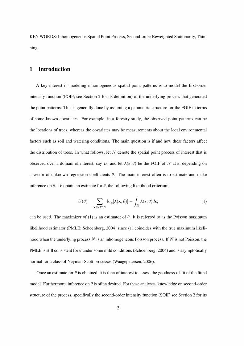
for estimator 3 was also very small. The small bias for estimators 1 and 2 was expected. Figure

1 plots the true K-function for the simulated processes and the K-function using the average of

the estimated parameters for estimator 3. Clearly the true K-function was approximated well when

λ = 200 and σ = .04 but not in the other three cases. This indicated that the magnitude of the bias

depended on how well the true second-order structure of the process was approximated by the fitted

model. For STD, estimator 1 generally had a slightly larger STD than estimator 2 when σ = .02

and/or λ = 200, but a smaller STD than estimator 3 when σ = .02. When λ = 200 and σ = .04,

the STD of estimator 3 was even smaller than that of estimator 2. When λ = 800 and σ = .04, the

STDs of all three estimators were comparable.

14

Tables 2 reports the mean squared errors (MSEs) for estimators 1-3 for both β = 1 and β = 2.

Generally, the MSE became larger when β increased for all three estimators except when x = .02.

This increased error was due to the increased variability in the estimation of the FOIF parameters.

For σ = .02, estimator 2 always had the smallest MSE, whereas estimator 3 had the largest. For

λ = 200 and σ = .04, estimator 3 often had the smallest MSE. This was expected in view of the

observations on the biases and the STDs in this case. For λ = 800 and σ = .04, estimator 1 surpris-

ingly even outperformed estimator 2. This was likely due to the large variability in the estimation

of the PCF in this case. In summary, the proposed variance estimation procedure performed only

slightly worse than the plug-in method when the correct PCF model was used but often much better

than the plug-in method when an incorrect but comparable model was used. In some situations, the

proposed procedure performed better even when the correct PCF model was used for the plug-in

method. In practice, it is almost impossible to determine what the correct PCF model is. Thus

the proposed procedure appears attractive in real applications, especially when there is doubt over

whether a fitted PCF model describes the second-order structure of the process adequately.

5 An Application to Real Data

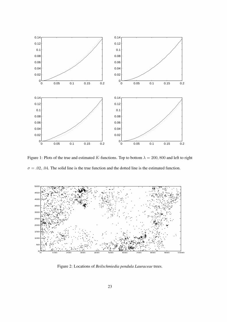
The data considered in this section consist of 3605 tree locations of the species Beilschmiedia pen-

dula Lauraceae (abbreviated by Beilschmiedia hereinafter) in a 1000 × 500 meters plot in Barro

Colorado Island (see Figure 2). Beilschmiedia is a perennial tree species that belongs to the Lau-

raceae Family. These locations were extracted from a much larger data set obtained in a 1995 cen-

sus, which contains measurements for over 300 species existing in the same plot. Waagepetersen

(2006) fit an INSP model to the data, using elevation and gradient as covariates. Specifically, the

15

FOIF of the model was defined as:

λ(s) = exp[β0 + β1E(s) + β2G(s)], (22)

where E(s) and G(s) were the (estimated) elevation and gradient at location s, respectively. In his

subsequent analysis, Waagepetersen concluded a significant effect for gradient but not for elevation.

Furthermore, the empirical K-function that he obtained agreed well with the fitted theoretical K-

function, which indicated an acceptable fit.

The empirical K-function also suggested that the Beilschmiedia trees were clustered. From a

biological point of view, the clustering might be caused by seed dispersal, which mostly likely had

occurred over multiple generations, or by correlation among other important environmental factors

(i.e. not elevation and gradient), which presumably also affected the distribution of Beilschmiedia.

The INSP model is used to model clustering due to the former. However, it is only a “crude

model” even in this sense since it considers seed dispersal only in one generation. As a result,

the INSP model may not be appropriate for the data. Although this does not necessarily invalidate

Waagepetersen’s conclusion, it would be of interest to further investigate these results under more

flexible conditions.

The data were analyzed here for three purposes: 1) to assess the goodness-of-fit of the fitted

model in Waagepetersen (2006), 2) to investigate any spatial trend in terms of the spatial coordinates

and 3) to make inference on the regression parameters β1 and β2. The first two purposes were not

considered by using the fitted FOIF directly in Waagepetersen (2006). For all analyses, (22) was

assumed to be the correct FOIF model but no specific assumption was made on the high-order

structure of the process other than it was SORWS. The residual diagnostics discussed in Section

3.1 was then used for the first two purposes, whereas the inferential procedure using subsampling

discussed in Section 3.2 was used for the third purpose.

16

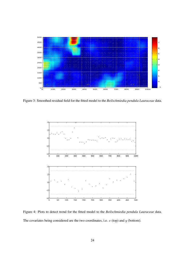
Figure 3 plots the standardized SRF that was based on the (unstandardized) SR in (19). The

set B in (19) was chosen to be a 80 × 80 meters square region, and the kernel function K(·)

was a uniform kernel over B. The variance for each SR was estimated by the proposed variance

estimation procedure, which was subsequently used to produce the standardized SRF. From Figure

3, the overall fit appeared to be good, except for one region that is centered around (300, 450)

meters. The standardized SRs in this region were much larger than as expected by the model.

This suggested that Beilschmiedia were more abundant in this region than could be attributed to

elevation and gradient alone. It appears sensible to suspect that other factors that were not included

in the model also affected the locations of Beilschmiedia. To identify these factors, it is necessary

to collect more covariates within this region. Furthermore, there appeared to be a possible problem

of overestimation of the FOIF for a large region in the center of the plot. This should also be

investigated in future studies.

Figure 4 plots the standardized SRFs by using each of the two coordinates as a covariate, where

the (unstandardized) SR used in each case to obtain the standardized SR was defined in (20). The

bandwidth h in (20) was set equal to 10 meters and the kernel function K(·) was a uniform kernel

over B(·, h). Again, the proposed variance procedure was applied to estimate the variance of each

SR so as to produce the standardized SRF. Figure 4 did not show a strong spatial trend in either

of the two coordinates. However, the plot against the x coordinate indicated one outlier around

x = 300. This provided further evidence for the conclusion that the outlying region suggested by

Figure 3 should be further investigated.

To make inference on β1 and β2, their 95% confidence intervals (CIs) were calculated by using

the inferential procedure in Section 3.2. The subblock size was 100×50 meters. Two other subblock

sizes (120 × 60 and 140 × 70 meters) were also considered and they both yielded similar results.

The initial variance estimate was equal to 0.017 for β1 and 2.119 for β2 by using the resampling

17

method in Guan and Loh (2006). The resulting CI was (−.015, .042) for β1 and (1.161, 10.225) for

β2. These results confirmed the conclusion of Waagepetersen (2006) that β2 was significant but β1

was not. Note that this was achieved under a much weaker assumption on the underlying process.

Appendix A: Proof of Theorem 1

For the ease of presentation, define

F (x) = f(x)λ(x), T ∗n,i(u) =∑

x∈Bn(u)∩N∗i

F (x−u), µn =∫

Bn

F (s)ds, and V ∗n = V ar

[T ∗n,i(u)

].

Consider the case b = 1. Note that V ∗n = |D∗

n|−1∫D∗n

[T ∗n,1(u)− µn

]2du is unbiased for V ∗

n . To

show that V ∗n

p→ V ∗n , it is only necessary to show that

Cn(u1,u2) =1

|Bn|2 Cov{[

T ∗n,1(u1)− µn

]2,[T ∗n,1(u2)− µn

]2}→ 0 as ||u1−u2|| → ∞ and n →∞.

Let µ2n = E

{[T ∗n,1(u)

]2}

. Note that

|Bn|2Cn(u1,u2) = E{[

T ∗n,1(u1)]2 [

T ∗n,1(u2)]2

}− 4µnE

{T ∗n,1(u1)

[T ∗n,1(u2)

]2}

+ 4(µn)2E[T ∗n,1(u1)T ∗n,1(u2)

]− (µ2n)2 + 4(µn)2µ2

n − 4(µn)4.

Note further that

[T ∗n,1(u)

]2 =∑∑

x1,x2∈Bn(u)

F (x1 − u)F (x2 − u),

T ∗n,1(u1)T ∗n,1(u2) =∑∑

x1∈Bn(u1),x2∈Bn(u2)

F (x1 − u1)F (x2 − u2),

T ∗n,1(u1)[T ∗n,1(u2)

]2 =∑

x1∈Bn(u1)

∑∑

x2,x3∈Bn(u2)

F (x1 − u1)F (x2 − u2)F (x3 − u2),

[T ∗n,1(u1)

]2 [T ∗n,1(u2)

]2 =∑∑

x1,x2∈Bn(u1)

∑∑

x3,x4∈Bn(u2)

F (x1−u1)F (x2−u1)F (x3−u2)F (x4−u2).

Thus by ignoring some multiplicative constants, |Bn|2Cn(u1,u2) can be written as the sum of the

following nine terms

∫

Bn(u1)∩Bn(u2)[F (x− u1)]

2 [F (x− u2)]2 dx,

18

∫

Bn(u1)

∫

Bn(u2)[F (x1 − u1)]

2 [F (x2 − u2)]2 g(x1 − x2)dx1dx2,

∫

Bn(u1)

∫

Bn(u1)∩Bn(u2)F (x1 − u1)F (x2 − u1) [F (x2 − u2)]

2 dx1dx2,

∫ ∫

Bn(u1)∩Bn(u2)

F (x1 − u1)F (x1 − u2)F (x2 − u1)F (x2 − u2)Q2(x1,x2)dx1dx2,

∫

Bn(u1)

∫ ∫

Bn(u2)

[F (x1 − u1)]2 F (x2 − u2)F (x3 − u2)Q3(x1,x2,x3)dx1dx2dx3,

∫

Bn(u1)∩Bn(u2)

∫

Bn(u1)

∫

Bn(u2)F (x1−u1)F (x1−u2)F (x2−u1)F (x3−u2)Q2(x2,x3)dx1dx2dx3,

∫

Bn(u1)∩Bn(u2)

∫

Bn(u1)

∫

Bn(u2)F (x1−u1)F (x1−u2)F (x2−u1)F (x3−u2)Q3(x1,x2,x3)dx1dx2dx3,

∫ ∫

Bn(u1)

∫ ∫

Bn(u2)

F (x1−u1)F (x2−u1)F (x3−u2)F (x4−u2)Q2(x1,x3)Q2(x2,x4)dx1dx2dx3dx4,

∫ ∫

Bn(u1)

∫ ∫

Bn(u2)

F (x1 − u1)F (x2 − u1)F (x3 − u2)F (x4 − u2)Q4(x1,x2,x3,x4)dx1dx2dx3dx4,

which are of order o(|Bn|2) as ||u1−u2|| → ∞ and n →∞ due to conditions (11) and (12). Thus

Theorem 1 is proved.

Appendix B: Proof of Corollary 1

Here consider only the case that µn(θn) = λ∗n(θn)∫Bn

f(s)λ(s; θn)ds. The proof for the case of

µn(θn) = [b|D∗n|]−1

∑bi=1

∫D∗n

T ∗i (u; θn)du follows similarly and thus is omitted. For the ease of

presentation, let F (x; θ) = f(x)λ(x; θ), λ∗n(θ) = mins∈Dn λ(s; θ), pn(x; θ) = λ∗n(θ)/λ(x; θ), and

N∗1 (θ) be a thinned realization of N∗

1 defined in (4), where λ(·) = λ(·; θ) is used to produce the

thinning probabilities.

Let r(x) be a uniform random variable in [0, 1]. If r(x) ≤ pn(x; θ), when x ∈ (N ∩Dn), then

x will be retained in N∗1 (θ). Based on the set {r(x) : x ∈ (N ∩Dn)}, we determine N∗

1 (θ0) and

N∗1 (θn). Define N∗

a = {x ∈ N∗1 (θ0),x /∈ N∗

1 (θn)} and N∗b = {x /∈ N∗

1 (θ0),x ∈ N∗1 (θn)}. Note

that P (x ∈ N∗a ∪N∗

b |x ∈ N) ≤ |pn(x; θn)− pn(x; θ0)|.

19

Define

µn(θ) = λ∗n(θ)∫

Bn

F (s; θ)ds,

T ∗n,1(u; θ) =∑

x∈Bn(u)∩N∗1 (θn)

F (x− u; θ),

T ∗n,0(u; θ) =∑

x∈Bn(u)∩N∗1 (θ0)

F (x− u; θ).

To prove Corollary 1, first note that

V ∗n (θn)− 1

|D∗n|

∫

D∗n[T ∗n,0(u; θ0)− µn(θ0)]2du

=1|D∗

n|∫

D∗n[T ∗n,1(u; θn)− T ∗n,1(u; θ0) + T ∗n,1(u; θ0)− T ∗n,0(u; θ0) + µn(θ0)− µn(θn)]2du

+2|D∗

n|∫

D∗n[T ∗n,0(u; θ0)− µn(θ0)][T ∗n,1(u; θn)− T ∗n,1(u; θ0) + T ∗n,1(u; θ0)− T ∗n,0(u; θ0)

+µn(θ0)− µn(θn)]du.

The above is of order o(|Bn|) in probability (i.p.) if the following are true:

(a) 1|D∗n||Bn|

∫D∗n

[T ∗n,1(u; θn)− T ∗n,1(u; θ0)]2dup→ 0,

(b) 1|D∗n||Bn|

∫D∗n

[T ∗n,1(u; θ0)− T ∗n,0(u; θ0)]2dup→ 0,

(c) 1|Bn| [µn(θ0)− µn(θn)]2 p→ 0

Condition (15) and the assumptions that f(·) is finite and λ(·, θ) has a bounded first-order derivative

imply that for all δ > 0 and 0 < α < 1, there exists C < ∞ such that

(a) ≤ Cδ

|D∗n|α+1|Bn|

∫

D∗n

[ ∑

N∩Bn(u)

1]2

du with probability 1.

The above converges to zero i.p. due to conditions (11) and (12).

To show (b), note that

T ∗n,1(u; θ0)− T ∗n,0(u; θ0) =∑

N∗b ∩Bn(u)

F (x− u; θ0)−∑

N∗a∩Bn(u)

F (x− u; θ0).

20

Thus there exists C < ∞ such that

(b) ≤ C

|D∗n||Bn|

∫

D∗n

[ ∑

N∗a∩Bn(u)

1]2

+[ ∑

N∗b ∩Bn(u)

1]2

du.

The above converges to zero i.p. due to the fact that P (x ∈ N∗a ∪ N∗

b |x ∈ N) ≤ C|Dn|α/2 i.p. The

latter is due to condition (15) and the smoothness condition on the FOIF assumed in Corollary 1.

Finally, note that (c) p→ 0 due to condition (15). Thus Corollary 1 is proved.

References

Baddeley, A. J., Møller, J. and Waagepetersen, R. (2000), “Non- and semi-parametric estimation of

interaction in inhomogeneous point patterns”, Statistica Neerlandica, 54, 329–350.

Baddeley, A. J., Turner, R., Møller, J. and Hazelton, M. (2005) “Residual analysis for spatial point

processes (with discussion)” Journal of the Royal Statistical Society, Series B, 67, 617–666

Brillinger, D. R. (1975), Time Series: Data Analysis and Theory, Holt, Rinehart & Winston.

Daley, D. J. and Vere-Jones, D. (1988), An Introduction to the Theory of Point Processes, New York:

Springer-Verlag.

Diggle, P. J. (2003), Statistical Analysis of Spatial Point Patterns, New York: Oxford University

Press Inc.

Guan, Y. and Loh, J. M. (2006), “A block bootstrap procedure in modeling inhomogeneous spatial

point patterns”, submitted.

Heinrich, L. (1985), “Normal convergence of multidimensional shot noise and rates of this conver-

gence”, Advances in Applied Probability, 17, 709–730.

McCullagh, P. (1987), Tensor Methods in Statistics, New York: Chapman and Hall.

21

Møller, J., Syversveen, A. R. and Waagepetersen, R. P. (1998), “Log Gaussian Cox processes”,

Scandinavian Journal of Statistics, 25, 451–482.

Møller, J. and Waagepetersen, R. P. (2003), Statistical Inference and Simulation for Spatial Point

Processes, New York: Chapman & Hall.

Papangelou, F. (1974), “The conditional intensity of general point processes and an application to

line processes”, Zeitschrift fr Wahrscheinlichkeitstheorie und verwandte Gebiete, 28, 207–226.

Politis, D. N. and Romano, J. P. (1994), “Large sample confidence regions based on subsamples

under minimal assumptions”, The Annals of Statistics, 22, 2031–2050.

Schoenberg, F. P. (2004), “Consistent parametric estimation of the intensity of a spatial-temporal

point process”, Journal of Statistical Planning and Inference, 128(1), 79–93.

Sherman, M. and Carlstein, E. (1996), “Replicate histograms”, Journal of the American Statistical

Association, 91, 566–576.

Stoyan, D. and Stoyan, H. (1994), Fractals, Random Shapes and Point Fields, New York: Wiley.

Waagepetersen, R. P. (2005), “Discussion of “Residual analysis for spatial point processes””, Jour-

nal of the Royal Statistical Society, Series B, 67, 662.

Waagepetersen, R. P. (2006), “An estimating function approach to inference for inhomogeneous

Neyman-Scott processes”, Biometrics, to appear.

22

0 0.05 0.1 0.15 0.20

0.02

0.04

0.06

0.08

0.1

0.12

0.14

0 0.05 0.1 0.15 0.20

0.02

0.04

0.06

0.08

0.1

0.12

0.14

0 0.05 0.1 0.15 0.20

0.02

0.04

0.06

0.08

0.1

0.12

0.14

0 0.05 0.1 0.15 0.20

0.02

0.04

0.06

0.08

0.1

0.12

0.14

Figure 1: Plots of the true and estimated K-functions. Top to bottom λ = 200, 800 and left to right

σ = .02, .04. The solid line is the true function and the dotted line is the estimated function.

0 100 200 300 400 500 600 700 800 900 10000

50

100

150

200

250

300

350

400

450

500

Figure 2: Locations of Beilschmiedia pendula Lauraceae trees.

23

0 100 200 300 400 500 600 700 800 900 10000

50

100

150

200

250

300

350

400

450

500

−1

0

1

2

3

4

5

6

7

Figure 3: Smoothed residual field for the fitted model to the Beilschmiedia pendula Lauraceae data.

0 100 200 300 400 500 600 700 800 900 1000−4

−2

0

2

4

0 50 100 150 200 250 300 350 400 450 500−4

−2

0

2

4

Figure 4: Plots to detect trend for the fitted model to the Beilschmiedia pendula Lauraceae data.

The covariates being considered are the two coordinates, i.e. x (top) and y (bottom).

24

Table 1: Bias and standard deviation (STD) of the variance estimator for the smoothed residual

defined in (19). Each bias and STD was divided by the estimated true variance of the residual.

Methods 1, 2, 3 are the proposed method, the plug-in method using the true PCF and the plug-in

method using an incorrect PCF, respectively.σ = .02 σ = .04

λ method x = .02 .04 .06 .08 .02 .04 .06 .08

BIAS 200 1 .027 -.075 -.030 .040 .047 .037 -.010 .0482 .037 -.066 -.019 .055 .035 .028 -.022 .0353 .102 -.002 .056 .143 .035 .028 -.023 .035

800 1 .010 -.027 -.034 .017 .018 .021 .004 .0192 .018 -.017 -.024 .029 .011 .011 -.003 .0113 .128 .101 .105 .177 .055 .061 .053 .074

STD 200 1 .296 .205 .214 .300 .271 .226 .228 .3092 .293 .196 .198 .295 .261 .216 .213 .2903 .318 .215 .219 .327 .260 .214 .210 .285

800 1 .169 .144 .151 .190 .164 .157 .171 .2092 .158 .133 .138 .183 .161 .155 .172 .2173 .181 .152 .159 .211 .164 .154 .170 .218

Table 2: Mean squared error (MSE) of the variance estimator for the smoothed residual defined in

(19). Each MSE was divided by the squared value of the estimated true variance of the residual.

Methods 1, 2, 3 are the proposed method, the plug-in method using the true PCF and the plug-in

method using an incorrect PCF, respectively.σ = .02 σ = .04

β λ method x = .02 .04 .06 .08 .02 .04 .06 .08

1 200 1 .088 .048 .047 .092 .076 .053 .052 .0982 .087 .043 .040 .090 .070 .047 .046 .0853 .112 .046 .051 .127 .069 .046 .045 .083

800 1 .029 .021 .024 .036 .027 .025 .029 .0442 .025 .018 .020 .034 .026 .024 .030 .0473 .049 .033 .036 .076 .030 .028 .032 .053

2 200 1 .083 .051 .059 .107 .072 .054 .072 .1622 .076 .044 .050 .102 .062 .045 .057 .1213 .089 .053 .067 .134 .062 .043 .054 .115

800 1 .027 .024 .031 .055 .023 .024 .035 .0642 .025 .021 .030 .053 .022 .027 .048 .1003 .041 .039 .057 .098 .022 .026 .048 .106

25