1

Vector Field Editing and Periodic Orbit ExtractionUsing Morse Decomposition

Guoning Chen, Konstantin Mischaikow, Robert S. Laramee, Pawel Pilarczyk, Eugene Zhang

Abstract— Design and control of vector fields is critical formany visualization and graphics tasks such as vector field visual-ization, fluid simulation, and texture synthesis. The fundamentalqualitative structures associated with vector fields are fixedpoints, periodic orbits, and separatrices. In this paper we providea new technique that allows for the systematic creation andcancellation of fixed points and periodic orbits. This techniqueenables vector field design and editing on the plane and surfaceswith desired qualitative properties.

The technique is based onConley theorywhich provides aunified framework that supports the cancellation of fixed pointsand periodic orbits. We also introduce a novel periodic orbitextraction and visualization algorithm that detects, for the firsttime, periodic orbits on surfaces. Furthermore, we describethe application of our periodic orbit detection and vector fieldsimplification algorithm to engine simulation data demonstratingthe utility of the approach.

We apply our design system to vector field visualizationby creating datasets containing periodic orbits. This helps usunderstand the effectiveness of existing visualization techniques.Finally, we propose a new streamline-based technique that allowsvector field topology to be easily identified.

Index Terms— Vector field design, vector field visualization,vector field topology, vector field simplification, Morse decompo-sition, Conley index, periodic orbit detection, connection graphs.

I. I NTRODUCTION

V ECTOR fields arise as models in almost all scientificand engineering endeavors which involve systems that

change continuously with time. In the case of two-dimensionalsystems that can be modelled by vector fields defined on sur-faces, visualization can play an important role in understandingthe essential features in the system. This is also true for two-dimensional vector fields that are linked to potentially noisydata, such as a velocity field extracted from experiments ornumerical simulations of fluids. In both cases, there are occa-sions in which one wishes to simplify the dynamic structurein a coherent admissible manner [1]. This latter step requiresthe ability to edit the underlying vector field. Furthermore,there are problems where the construction and modificationof a vector field represents a preliminary step towards a largergoal such as texture synthesis [2], [3], [4] and fluid simulationfor special effects [5].

There is substantial literature on the subject of vector fieldtopology extraction and simplification, with considerable focuson the identification and manipulation offixed points(see [6]and references therein). On the other hand,periodic orbitsareessential structures ofnon-gradientvector fields, such as thosein electromagnetism, chemical reactions, fluid dynamics, loco-motion control, population modelling, and economics. Thereis a fundamental need to be able to incorporate them into the

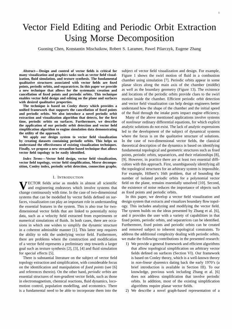
subject of vector field visualization and design. For example,Figure 1 shows the swirl motion of fluid in a combustionchamber using simulation [7]. Periodic orbits appear in someplanar slices along the main axis of the chamber (middle)as well as the boundary geometry (Figure 13). The existenceand locations of the periodic orbits provide clues to the swirlmotion inside the chamber. Efficient periodic orbit detectionand vector field visualization can help design engineers betterunderstand how the shape of the chamber and the initial speedof the fluid through the intake ports impact engine efficiency.

Many of the above mentioned applications involve systemsof nonlinearordinary differential equations, for which explicitanalytic solutions do not exist. The lack of analytic expressionsled to the development of the subject of dynamical systemswhere the focus is on the qualitative structure of solutions.In the case of two-dimensional vector fields, the classicaltheoretical description of the dynamics is based on identifyingfundamental topological and geometric structures such as fixedpoints, periodic orbits, separatrices, and their relationships [8],[9]. However, in practice there are at least two essential diffi-culties with this approach. First, unambiguously identifying allthe topological structures for an arbitrary system is impossible.For example, Hilbert’s 16th problem, that of bounding thenumber of isolated periodic orbits for a polynomial vectorfield on the plane, remains essentially unsolved [10]. Second,the existence of noise reduces the importance of objects suchas fixed points and periodic orbits.

In this paper, we develop a vector field visualization anddesign system that extracts and visualizes boundary flow topol-ogy. This includes analyzing and modifying the vector field.The system builds on the ideas presented by Zhang et al. [6],and it provides the user with a variety of capabilities in thatfixed points, periodic orbits, and separatrices can be identified.Furthermore, fixed points and periodic orbits can be createdand removed subject to inherent topological constraints. Toaddress the additional complexity dealing with periodic orbits,we make the following contributions in the presented research:

1) We provide a general framework and efficient algorithmsthat allow topological simplification on arbitrary vectorfields defined on surfaces (Section VI). Our frameworkis based on Conley theory, which is a well-known theoryin non-linear dyanmicsdating back the early1970’s (abrief introduction is available in Section III). To ourknowledge, previous work including Zhang et al. [6]does not address simplification that involve periodicorbits. In addition, most of the existing simplificationalgorithms require planar vector fields.

2) We describe a novel graph-based representation of a

2

Fig. 1. Visualizing the simulation of flow in a diesel engine: the combustion chamber (leftmost) and four planar slices of the flow inside the chamberfor which the plane normals are along the main axis of the chamber. From left to right are slices cut at10%, 25%, 50%, and 75% of the length of thecylinder from the top where the intake ports meet the chamber. The vector fields are defined as zeros on the boundary of the geometry (no-slip condition).The automatic extraction and visualization of flow topology allows the engineer to gain insight into where the ideal pattern of swirl motion is realized insidethe combustion chamber. In fact, the behavior of the flow and its associated topology, including periodic orbits, is much more complicated than the ideal.Figure 13 provides complementary visualization of the flow on the boundary of the diesel engine.

vector field based on Morse decomposition, which werefer to asMorse Connection Graphs(MCG). This graphcontains supplementary information with respect to thewell-known vector field skeletonin that it addressesperiodic orbits. We also provide an algorithm to effi-ciently compute MCG as well as their refinement (EntityConnection Graphics, or ECG) (Section V-B).

3) Our system allows a user to create periodic orbits onsurfaces (Section IV). To do so, we combine the ideasof basis vector fields and constraint optimization. To ourknowledge, this is the first time a periodic orbit creationalgorithm is proposed and implemented.

4) As part of MCG and ECG construction, we presenta novel and practical algorithm for periodic orbit ex-traction without first having to compute separatrices(Section V-A). Our method is based on the topologicaland geometric analysis of a vector field, and it enablesextraction of periodic orbits–even those that are notaccessible via saddle points.

5) The utility of our topological analysis, including periodicorbit detection and vector field simplification, is demon-strated in the context of a novel application, namely, thevisualization of in-cylinder flow from automotive enginesimulation data (Sections V and VI). Our algorithm forperiodic orbit detection and ECG construction only takesless than a minute on one such dataset with nearly900,000 triangles.

6) We propose an enhanced streamline-based method inwhich periodic orbits and separatrices are highlighted inthe display (Section VII). This is particularly desirablefor vector fields on surfaces since only portions of aperiodic orbit may be visible for any given viewpoint(Figure 6).

Because of the essential mathematical difficulties mentionedearlier, our numerical methods do not focus directly on fixedpoints, periodic orbits, and separatrices. Rather, we employtechniques based on Conley’s purely topological approach todynamical systems [11]. Broadly speaking, our approach isbased on three steps. The first is to identify regions on whichthe dynamics exhibits recurrent behavior, i.e. fixed points andperiodic orbits, and/or gradient-like behavior, i.e. separatrices.This involves the construction ofMorse decompositions. Atheoretical computational foundation for the types of algo-

rithms we employ can be found in [12], [13]. The second isto identify the type of dynamics occuring in these regions, i.e.the existence of fixed points, periodic orbits, and separatrices.This is done using numerical methods and theConley index. Itshould be noted that the Conley index not only generalizes thePoincare index as it applies to fixed points, but it also providesinformation about the existence of periodic orbits. Finally, thevector field is modified in the identified regions to produce thedesired dynamics.

The rest of the paper is organized as follows: Section IIprovides a brief review of related work on topology-basedvector field visualization. In Section III, we review relatedwork and introduce Conley theory. Section IV introduces ourmethod for creating periodic orbits on the plane and surfaces.Section V describes our periodic orbit detection technique andprovides an algorithm for the construction of the MCG andECG of a vector field. We present a general algorithm for var-ious cancelling operations in Section VI. Section VII providesdetails on our enhanced streamline based flow visualizationtechnique followed by a discussion of possible future work inSection VIII.

II. RELATED WORK

Vector field visualization, analysis, simplification, and de-sign have received much attention from the Visualizationcommunity over the past twenty years. Much excellent workexists, and to review it all is beyond the scope of this paper.Here, we only refer to the most relevant work. Interestedreaders can find a complete survey in [14], [15], [16].

A. Vector Field Design

There has been some work in creating vector fields onthe plane and surfaces, most of which is for graphics ap-plications such as texture synthesis [2], [3], [4] and fluidsimulation [5]. These methods do not address vector fieldtopology, such as fixed points. There are a few vector fielddesign systems that make use of topological information. Forinstance, Rockwood and Bunderwala [17] use ideas fromgeometric algebra to create vector fields with desired fixedpoints. Van Wijk [18] develops a vector field design systemto demonstrate his image-based flow visualization technique(IBFV). The basic idea of this system is the use of basis vectorfields that correspond to various types of fixed points. Thissystem is later extended to surfaces [19], [20]. None of these

3

methods provide explicit control over the number and locationof fixed points since unspecified fixed points may appear.Theisel [21] proposes a planar vector field design system inwhich the user has complete control over fixed points andseparatrices. However, this requires the user to provide thecompletetopological skeletonof the vector field, which canbe labor-intensive. Recently, Zhang et al. [6] develop a designsystem for both planar domains and surfaces. This systemprovides explicit control over the number and location of fixedpoints throughfixed point pair cancellationand movementoperations. Our work is inspired by their system. However,we enable automatic extraction and visualization of periodicorbits on surfaces. We also introduce topology simplificationoperations for periodic orbits. There has also been recent workby Weinkauf et al. [22] on the design of 3D vector fields.

B. Vector Field Topology and Analysis

Helman and Hesselink [23] introduce vector field topologyfor the visualization of vector fields. They also propose ef-ficient algorithms to extract vector field topology. Followingtheir footsteps, much research has been conducted in topo-logical analysis of vector fields. For example, Scheuermannet al. [24] use clifford algebra to study the non-linear fixedpoints of a vector field and propose an efficient algorithmto merge nearby first-order fixed points. Tricoche et al. [1]and Polthier and Preuβ [26] give efficient methods to locatefixed points in a vector field. Wischgoll and Scheuermann [27]develop a method to extract closed streamlines in a 2D vectorfield defined on a triangle mesh. Note that closed streamlinesare in fact attracting and repelling periodic orbits. Theisel etal. [28] propose a mesh-independent periodic orbit detectionmethod for planar domains. In contrast to these approaches,our automatic detection algorithm is extended to surfaces.Furthermore, this is the first time periodic orbit extraction andvisualization has found utility in a real application.

C. Vector Field Simplification

Vector field simplification refers to reducing the complex-ity of a vector field. There are two classes of simplifi-cation techniques: topology-based (TB), and non-topology-based (NTB) [6]. Existing NTB techniques are usually basedon performing Laplacian smoothing on the potential of avector field inside the specified region. One example of thesework is by Tong et al. [29], who decompose a vector fieldusing Hodge-decomposition and then smooth each-componentindependently before summing them. TB techniques simplifythe topology of a vector field explicitly. Tricoche et al. [1]simplify a planar vector field by performing a sequence ofcancelling operations on fixed point pairs that are connected bya separatrix. They refer to this operation aspair annihilation.A similar operation, namedpair cancellation, has been usedto remove a wedge and trisector pair in a tensor field [30].We will follow this convention and refer to such an operationas fixed point pair cancellation. Zhang et al. [6] provide afixed point pair cancellation method based on Conley theory.They also extend this operation to surfaces and to fixed pointpairs that arenot connected by a separatrix, such as a centerand saddle pair. In this paper, we describe a more general

framework for cancelling object pairs such as fixed points andperiodic orbits (Section VI).

III. B ACKGROUND ON VECTORFIELDS

Our control of vector fields on surfaces is done usingconcepts from the topological theory of dynamical systems.Consider a manifoldM and a subsetX ⊂M. The boundary ofX is denoted by∂X and closure bycl(X).

Mathematically, a vector field can be expressed in termsof a differential equationx = V(x). The set of solutions toit gives rise to aflow on M; that is a continuous functionϕ : R×M →M satisfyingϕ(0,x) = x, for all x∈M, and

ϕ(t,ϕ(s,x)) = ϕ(t +s,x) (1)

for all x∈M and t,s∈ R. Given x∈M, its trajectory is

ϕ(R,x) := ∪t∈Rϕ(t,x). (2)

S⊂M is an invariant setif ϕ(t,S) = S for all t ∈R. Observethat for everyx ∈ M, its trajectory is an invariant set. Othersimple examples of invariant sets include the following. Apoint x∈M is a fixed pointif ϕ(t,x) = x for all t ∈ R. Moregenerally, x is a periodic point if there existsT > 0 suchthat ϕ(T,x) = x. The trajectory of a periodic point is called aperiodic orbit.

Consideration of the important qualitative structures as-sociated with vector fields on a surface requires familiaritywith hyperbolic fixed points, period orbits and separatrices.Let x0 be a fixed point of a vector fieldx = V(x); thatis V(x0) = 0. The linearization ofV about x0, results in a2× 2 matrix D f (x0) which has two (potentially complex)eigenvaluesσ1 + iµ1 and σ2 + iµ2. If σ1 6= 0 6= σ2, thenx0 iscalled ahyperbolic fixed point. Observe that on a surface thereare three types of hyperbolic fixed points:sinks σ1,σ2 < 0,saddlesσ1 < 0 < σ2, andsources0 < σ1,σ2. Because we areconsidering systems with invariant sets such as periodic orbits,the definition of the limit of a solution with respect to time isnon-trivial. Thealpha andomega limit setsof x∈M are

α(x) := ∩t<0cl(ϕ((−∞, t),x)), ω(x) := ∩t>0cl(ϕ((t,∞),x))

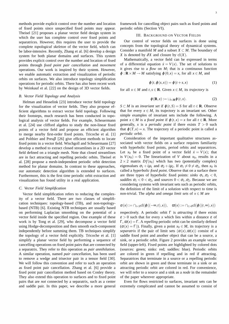
respectively. A periodic orbitΓ is attracting if there existsε > 0 such that for everyx which lies within a distanceε ofΓ, ω(x) = Γ. A repellingperiodic orbit can be similarly defined(α(x) = Γ)). Finally, given a pointx0 ∈M, its trajectory is aseparatrix if the pair of limit sets(α(x),ω(x)) consist of asaddle fixed point and another object that can be a source, asink, or a periodic orbit. Figure 2 provides an example vectorfield (upper-left). Fixed points are highlighted by colored dots(sources: green; sinks: red; saddles: blue). Periodic orbitsare colored in green if repelling and in red if attracting.Separatrices that terminate in a source or a repelling periodicorbit are shown in green and those terminate in a sink or anattracting periodic orbit are colored in red. For convenience,we will refer to a source and a sink as anodein the remainderof the paper wherever appropriate.

Even for flows restricted to surfaces, invariant sets can beextremely complicated and cannot be assumed to consist of

4

Fig. 2. An example vector field (upper left) and its ECG (lower left). Thevector field contains a source (green), three sinks (red), three saddles (blue),a repelling periodic orbit (green), and two attracting periodic orbits (red).Separatrices that connect a saddle to a repeller (a source or a periodic orbit) arecolored in green, and to an attractor (a sink or a periodic orbit) are colored inred. The fixed points and periodic orbits are the nodes in the ECG (lower left)and separatrices are the edges. In addition, a periodic orbit can be connecteddirectly to a source, sink, or another periodic orbit. Such connections are alsodepicted as edges in the ECG. The simplified field of (upper left) is shown in(upper right) and its corresponding ECG is (lower right). Notice the Conleyindex for both vector fields inside the white loop are the same, which allowsthe vector field in the left to be simplified into the one shown in the right.

hyperbolic fixed points, periodic orbits and separatrices [31].Furthermore, even if the recurrent dynamics is restricted tofixed points and periodic orbits, it is impossible to developan algorithm that will identify all of them. For example, itis easy to generate vector fields that contain infinitely manyisolated fixed points and/or periodic orbits. Thus we requirea language that allows us to manipulate a broader but usefulclass of invariant sets.

A. Morse Decomposition and Connection Graphs

A compact setN ⊂ M is an isolating neighborhoodiffor all x ∈ ∂N, ϕ(R,x) 6⊂ N. That is, the flow enters orleavesN eventually everywhere on∂N. An invariant setSis isolated if there exists an isolating neighborhoodN suchthat S is the maximal invariant set contained inN. Observethat hyperbolic fixed points and periodic orbits are examplesof isolated invariant sets. Isolated invariant sets posses twoessential properties. First, there are efficient algorithms foridentifying isolating neighborhoods [12]. Second, there existsan index, called the Conley index [32], that identifies the typesof modifications to the structure of the invariant set that aretopologically permissible. For example, the Conley index ofthe vector field shown in Figure 2 (upper-left) inside the whiteloop is identical to that of a sink. Topological simplificationof the complex field inside the region can result in the fieldshown in the right.

Central to our effort is the need for a computationally ro-bust decomposition of invariant sets. AMorse decomposition,M (S), of S consists of a finite collection of isolated invariantsubsets ofS, calledMorse sets,

M (S) := {M(p) | p∈P} (3)

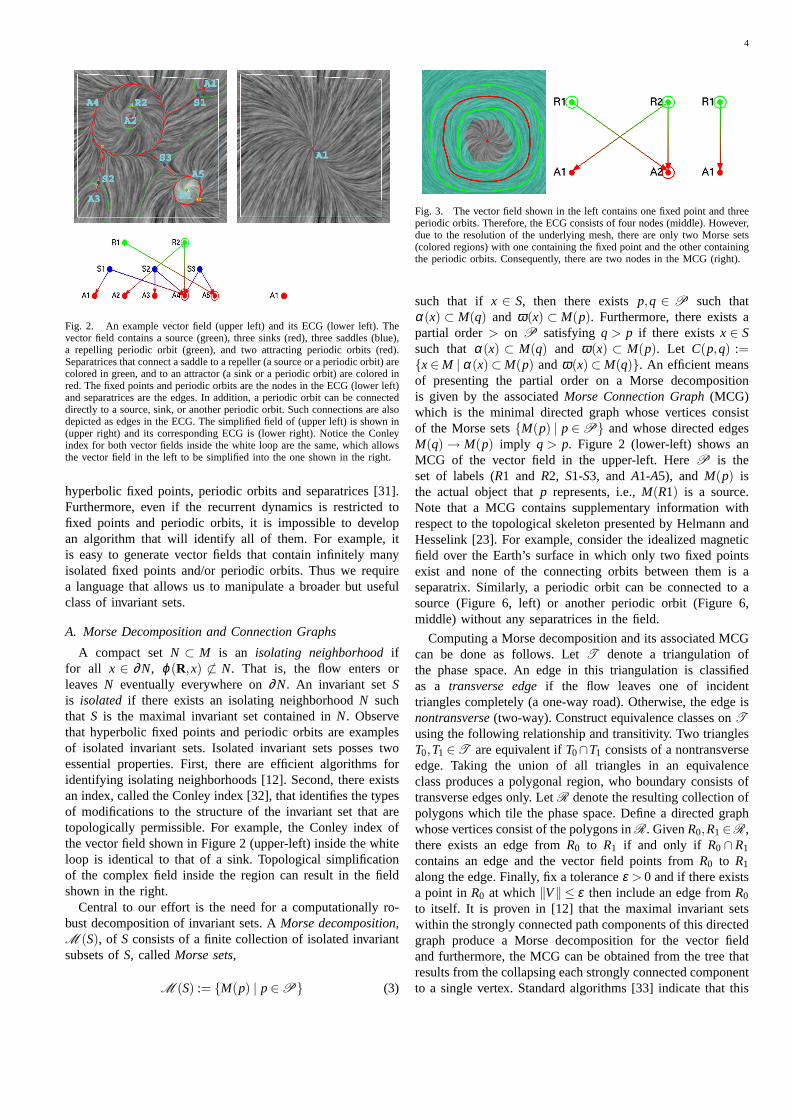
Fig. 3. The vector field shown in the left contains one fixed point and threeperiodic orbits. Therefore, the ECG consists of four nodes (middle). However,due to the resolution of the underlying mesh, there are only two Morse sets(colored regions) with one containing the fixed point and the other containingthe periodic orbits. Consequently, there are two nodes in the MCG (right).

such that if x ∈ S, then there existsp,q ∈ P such thatα(x) ⊂ M(q) and ω(x) ⊂ M(p). Furthermore, there exists apartial order> on P satisfying q > p if there existsx ∈ Ssuch thatα(x) ⊂ M(q) and ω(x) ⊂ M(p). Let C(p,q) :={x∈M | α(x)⊂M(p) andω(x)⊂M(q)}. An efficient meansof presenting the partial order on a Morse decompositionis given by the associatedMorse Connection Graph(MCG)which is the minimal directed graph whose vertices consistof the Morse sets{M(p) | p∈P} and whose directed edgesM(q) → M(p) imply q > p. Figure 2 (lower-left) shows anMCG of the vector field in the upper-left. HereP is theset of labels (R1 and R2, S1-S3, and A1-A5), and M(p) isthe actual object thatp represents, i.e.,M(R1) is a source.Note that a MCG contains supplementary information withrespect to the topological skeleton presented by Helmann andHesselink [23]. For example, consider the idealized magneticfield over the Earth’s surface in which only two fixed pointsexist and none of the connecting orbits between them is aseparatrix. Similarly, a periodic orbit can be connected to asource (Figure 6, left) or another periodic orbit (Figure 6,middle) without any separatrices in the field.

Computing a Morse decomposition and its associated MCGcan be done as follows. LetT denote a triangulation ofthe phase space. An edge in this triangulation is classifiedas a transverse edgeif the flow leaves one of incidenttriangles completely (a one-way road). Otherwise, the edge isnontransverse(two-way). Construct equivalence classes onTusing the following relationship and transitivity. Two trianglesT0,T1 ∈T are equivalent ifT0∩T1 consists of a nontransverseedge. Taking the union of all triangles in an equivalenceclass produces a polygonal region, who boundary consists oftransverse edges only. LetR denote the resulting collection ofpolygons which tile the phase space. Define a directed graphwhose vertices consist of the polygons inR. GivenR0,R1∈R,there exists an edge fromR0 to R1 if and only if R0∩R1

contains an edge and the vector field points fromR0 to R1

along the edge. Finally, fix a toleranceε > 0 and if there existsa point inR0 at which‖V‖ ≤ ε then include an edge fromR0

to itself. It is proven in [12] that the maximal invariant setswithin the strongly connected path components of this directedgraph produce a Morse decomposition for the vector fieldand furthermore, the MCG can be obtained from the tree thatresults from the collapsing each strongly connected componentto a single vertex. Standard algorithms [33] indicate that this

5

procedure can be performed in linear time in the number ofvertices and edges in the graph.

A node in the MCG is an isolated invariant set, whichmay contain multiple fixed points and periodic orbits. Formany engineering applications, such as the study of in-cylinderflow, engineers are often more concerned with individual fixedpoints and periodic orbits. Therefore, there is a need to builda graphG , whose nodes consist of fixed points and periodicorbits. Similar to an MCG, the edges inG represents theconnectivity information between the nodes according to thevector field. We refer to this graph as anEntity ConnectionGraph, or ECG. An ECG is a refinement of the MCG of thesame vector field. In fact, an MCG can be obtained from thecorresponding ECG by merging nodes that are in the sameMorse set. Furthermore, the MCG is equal to the ECG whenthe vector field has a finite number of fixed points and periodicorbits, all of which have an isolating neighborhood of theirown. In the remainder of the paper, we will only show theECG’s for illustration purposes.

Given that the ECG is a refinement of the MCG, the readermay wonder why we emphasize the existence of both graphs.There are two reasons. The first is that we make use ofinformation from the MCG to compute the ECG. The secondhas to do with the validity of the information. Any numericalor experimental method is subject to errors and thus onemust be concerned with whether these errors are significantenough to produce misleading information. In the domain ofnumerical analysis the existence of spurious solutions wouldbe an example of such misleading information. A rigorousanalysis of the validity of the methods being presented hereis beyond the scope of this paper, however we believe thatas a basis for future research it is important to point out thatthe topological methods of Conley theory have been used toobtain computer assisted, but mathematically rigorous proofsconcerning the structure of a wide variety nonlinear dynamicalsystems [34], [35]. Thus, our confidence level in the validity ofthe visualized structures and modifications is higher for thoseobjects identified with the MCG than the ECG.

B. Vector Field Simplification on Surfaces

Vector field simplification corresponds to a reduction in thenumber of Morse sets in the decomposition (compare the twofields in Figure 2). Vector field modification corresponds toa change in the dynamics within an isolating neighborhoodof a Morse set. To foreshadow the discussion of Section VIand to understand the potential vector field simplification thatcould possibly be associated with such a reduction requiresthe introduction of a topological invariant, the Conley index.

While the Conley index is applicable in the setting of ageneral dynamical system, we restrict our attention to thesetting of flows on surfaces. An isolating neighborhoodN isan isolating block if there existsε > 0 such that for everyx∈ ∂N, we have

ϕ((−ε,0),x)∩N = /0 or ϕ((0,ε),x)∩N = /0

In other words, the trajectory entersN, leavesN, or bothimmediately everywhere on∂N. The exit setof an isolating

block N is L := {x∈ ∂N | ϕ((0,ε),x)∩N = /0}. The pair(N,L)is called anindex pair. In [12] it is proven that the sets in phasespace which correspond to the strongly connected componentsare isolating blocks for the flowϕ associated with the vectorfield V.

Let S be the maximal invariant set in the isolating blockN with exit set L. The Conley indexof S is the relativehomology [36] of the index pair(N,L); that is, CH∗(S) :=H∗(N,L) (see Appendix for more details). Because we arerestricting our attention to flows on orientable surfaces, it issufficient to remark that we can writeCH∗(S) = (β0,β1,β2) ∈Z3 where βi represents thei-th Betti number ofH∗(N,L).It should be remarked that algorithms for computing Bettinumbers exist [36] and thus we need not concern ourselveswith these issues.

C. Important Conley Indices

Returning to the topic of design, the most important Conleyindices are as follows:

x0 an attracting fixed point ⇒ CH∗(x0) = (1,0,0)x0 a saddle fixed point ⇒ CH∗(x0) = (0,1,0)

x0 a repelling fixed point ⇒ CH∗(x0) = (0,0,1)Γ an attracting periodic orbit⇒ CH∗(Γ) = (1,1,0)

Γ a repelling periodic orbit ⇒ CH∗(Γ) = (0,1,1)S= /0 ⇒ CH∗(S) = (0,0,0)

Observe that the emptyset is by definition an isolated invariantset. (0,0,0) represents the index information for a region inwhich every point leaves in both forward and backward time. Itshould be noted that the reverse implications are not true. Forexample, given a polygonal index pair(N,L) for a vector fieldV, if H∗(N,L) = (0,0,0), then one cannot conclude that themaximal invariant set incl(N\L) is the empty set. However,it can be proven that there does exist a different vector fieldV such thatV = V on ∂ (cl(N \L)) and the empty set is themaximal invariant set incl(N \L) under the flow induced byV. Note the Poincare index for an attracting fixed point is thesame as a repelling one. Furthermore, the Poincare index fora periodic orbit is zero, which equals that of an emptyset.Therefore, Poincare index theory does not provide enoughutility to handle periodic orbits, thus limiting its potential uses.

To make it clear how the Conley index information canbe used in the vector field design process, let us reviewour strategy. The first step is the identification of a Morsedecomposition for the entire flow. Given the associated MCG,the user identifies an interval that contains the elements whichare to be eliminated. The interval defines an isolated invariantset for which an appropriate isolating block is constructed.The Conley index is then computed. This index informationprovides a topological constraint on the possible simplificationor modification of the vector field within the isolating block.For example, if the Conley index does not equal(0,0,0), thenany modification will result in the existence of a nontrivialinvariant set. To provide an even more specific example, if theConley index is that of a fixed point, then any modificationof the dynamics on the region will result in a vector field

6

that possess at least one fixed point. Further examples will beprovided in Section VI.

D. Vector Field Representation

We now describe the computational model of our system.In this model, the underlying domain is represented by a trian-gular mesh. Vector values are defined at the vertices only, andinterpolation is used to obtain values on the edges and insidetriangles. This applies to vector field editing, simplification,and analysis such as fixed point and periodic orbit extraction.

For the planar case, we use the popular piecewise linearinterpolation method [1]. On curved surfaces, we borrow theinterpolation scheme of Zhang et al. [6], which guarantees vec-tor field continuity across the vertices and edges of the mesh.These interpolation schemes support efficient flow analysisoperations on both planes and surfaces.

E. Constrained Optimization

One of the essential operations in our system is constrainedoptimization, which refers to solving a vector-valued discreteLaplacian equation over a regionN in the domain (a triangularmesh) where the vector values at the boundary vertices ofNare the constraints. This operation is used to create periodicorbits (Section IV) and to perform topological simplification(Section VI). The equation has the following form:

V(vi) = ∑j∈J

ωi jV(v j) (4)

where vi is an interior vertex,v j ’s are the adjacent verticesthat are either in the interior or on the boundary ofN, andVrepresents the vector field. The weightsωi j ’s are determinedusing Floater’s mean-value coordinates [37]. Equation 4 is asparse linear system, which we solve by using a conjugategradient method [38]. For convenience, we refer to a vertexvas beingfixedif the vector value atv is part of the constraints.Otherwise,v is free. Note that a similar formulation has beenused to reduce the complexity of vector fields [6] and tensorfields [39].

IV. PERIODIC ORBIT CREATION

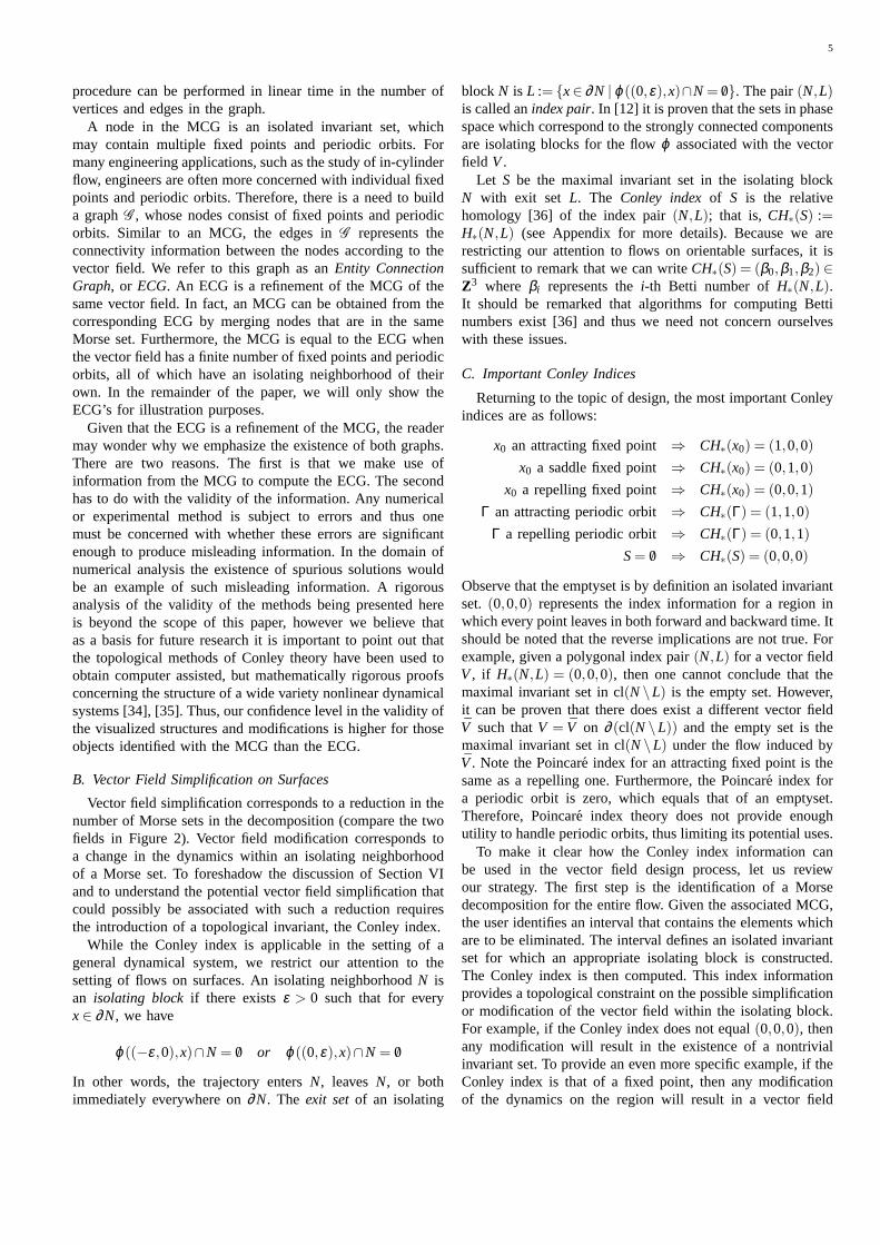
In this section, we describe novel algorithms for creatingperiodic orbits in the plane and on surfaces. The input to ouralgorithms consists of the desired type of the orbit (attractingor repelling) and a prescribed path, which is an oriented loop.Figure 4 shows an example path (left: blue loop). We thengenerate a sequence of evenly-spaced sample points on theloop (middle: green dots) and treat the tangent vectors atthese points as constraints (middle: magenta arrows). Finally,we produce a vector field with a periodic orbit that closelymatches the user input (right: red dashed lines). We use thedashed lines to represent the continuous periodic orbit so thatit can be visually compared with the user-specified path. Next,we describe two ways of creating a vector field based on theconstraints: basis vector fields and constrained optimization.

Fig. 4. Given an oriented loop (left), our system produces a sequence ofsample points (middle: dots) and evaluates tangent vectors at those locations(middle: arrows). We then compute a vector field that contains a periodicorbit (right: red dashed lines) by generating constraints based on these vectorvalues. Notice that the periodic orbit matches closely the user-specified loop.

A. Attracting and Repelling Basis Vector Fields

An intuitive way to build a vector field that satisfies theconstraints is to use basis vector fields. This idea has beenapplied to creating wind forces to guide computer anima-tion [40], to testing a vector field visualization technique [18],and to generating vector fields for non-photorealistic renderingand texture synthesis [6]. In this case, the constraints arealso referred to asregular design elements[6]. Each regularelement is used to produce a globally definedbasis vectorfield that has a constant direction with decreasing magnitudeas one moves away from the center of the element. Withproperly chosen blending functions, the weighted sum of thebasis vector fields satisfies all the constraints.

In theory, any vector field can be created by using regularelements. In practice, however, it often requires an excessivenumber of regular elements to generate certain vector fieldfeatures. For example, at least three regular elements areneeded to specify a source or a center. To produce a periodicorbit, regular elements must be specified not only along theprescribed path, but also near the orbit in order to enforcethe type of the orbit (attracting or repelling). Given that thecost of summing basis vector fields is proportional to thenumber of design elements, we wish to reduce the numberof basis vector fields while maintaining efficient control. Thisis achieved with the introduction of two new types of designelements:attachment elementsandseparation elements.

Before describing these elements, we briefly review theconcepts of attachment and separation points from Ken-wright [25]. Given a vector fieldV and a pointp0 in theplane, we consider the following two values:e1×u ande2×u,whereu is the vector value atp0 ande1 ande2 are the majorand minor eigenvectors of the Jacobian.p0 is an attachmentpoint if e1×u = 0, and aseparation pointif e2×u = 0. Anattachment line consists of attachment points. Geometrically,such a line attract nearby flow. A separation line can bedefined in a similar fashion except that nearby flow is repelledfrom the curve. Ideally, an attachment element will result in abasis vector field that has an attachment line as illustratedin Figure 5 (middle). The following formula describes anattachment element that has a desired vector value of(1,0)at (x0,y0).

V(x,y) = B(x,y)(

1c(y−y0)

)(5)

whereB(x,y) = e−((x−x0)2+(y−y0)2) is the blending function forthe element andc < 0 is a parameter that describes the speed

7

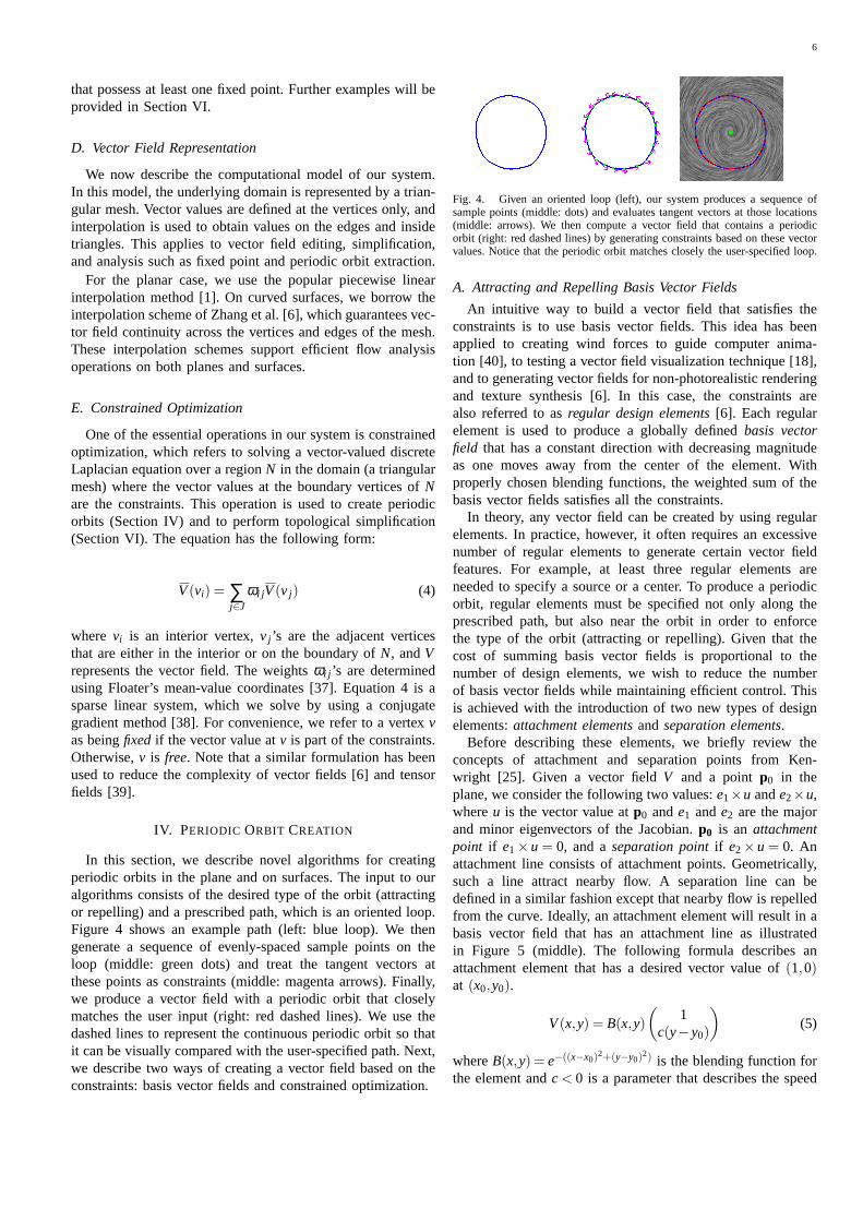
Fig. 5. This figure compares the basis vector field corresponding to a regularelement (left) and an attachment element (middle). The periodic orbit in theright was created by using four attachment elements.

at which the flow leaves the liney = y0. The larger|c| is,the more quickly the vectors near the attachment line pointtowards it. Notice the basis field contains an attachment lineat y = y0. Formula 5 can also be used to specify a separationelement (c> 0) and a regular element (c= 0). When the vectorvalue is(cosθ0,sinθ0) for some constantθ0, the formula hasthe following form:

V(x,y) = B(x,y)((

cosθ0

sinθ0

)+cP(x,y)

(−sinθ0

cosθ0

)) (6)

whereP(x,y) =−sinθ0(x−x0)+cosθ0(y−y0) is the signeddistance of a point(x,y) to the line that is specified bythe location and direction of the design element. Figure 5compares two basis vector fields generated from a regularelement (left) and an attachment element (middle). The rightimage shows an attracting periodic orbit created from fourattachment elements. The ideas of attachment and separationwill be used again in our periodic orbit extraction algorithm(Section V-A).

Vector field design using basis vector fields is intuitive andgenerates smooth results. However, the cost associated withthis approach is proportional to the number of basis vectorfields. To specify a relative large periodic orbit with highcurvature often requires hundreds of attachment or separationelements, which makes interactive design a difficult task. Theproblem is magnified on surfaces on 3D as every basis vectorfield requires a global surface parameterization that is specificto the underlying design element [6]. Constructing hundredsof surface parameterizations makes it impractical to createa periodic orbit interactively. Next, we describe a differentstrategy that is based on constrained optimization.

B. Constrained Optimization for Periodic Orbit Creation

Given a user-specified oriented loopγ and the desiredtype of the periodic orbit, our system performs the followingoperations to create a periodic orbit that closely matches theinput.

First, we identify a regionRγ , which is a set of trianglesthat encloseγ. Next, we assign vector values to the verticesof Rγ according to the desired type, path, and orientation ofthe periodic orbit. Finally, our system performs a constrainedoptimization to compute vector values for vertices outsideRγ ,i.e., the free vertices in the domain. The quality of the resultingperiodic orbit depends on the choice ofRγ and the vectorassignment on the boundary ofRγ .

We reuse attachment and separation elements to obtainvector values onRγ . Basically, each line segment on theloop γ is used to infer a design element. We then compute

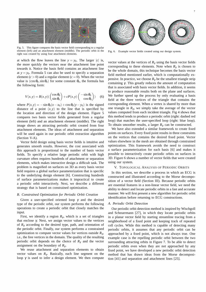
Fig. 6. Example vector fields created using our design system.

vector values at the vertices ofRγ using the basis vector fieldscorresponding to these elements. Note whenRγ is chosen tobe the whole domain, this technique becomes the basis vectorfield method mentioned earlier, which is computationally ex-pensive. In practice, we chooseRγ be the smallest triangle stripcontainingγ. This greatly reduces the amount of computationthat is associated with basis vector fields. In addition, it seemsto produce reasonable results both on the plane and surfaces.We further speed up the process by only evaluating a basisfield at the three vertices of the triangle that contains thecorresponding element. When a vertex is shared by more thanone triangle inRγ , we simply take the average of the vectorvalues computed from each incident triangle. Fig 4 shows thatthis method tends to produce a periodic orbit (right: dashed redloop) that matches the user-specified loop (right: blue loop).To obtain smoother results, a largerRγ can be constructed.

We have also extended a similar framework to create fixedpoints on surfaces. Every fixed point results in three constraintson the vertices that contains the desired fixed point. Vectorvalues elsewhere in the mesh are obtained through constrainedoptimization. This framework avoids the need to constructa surface parameterization for each basis [6] and makes itpossible to interactively create periodic orbits on surfaces in3D. Figure 6 shows a number of vector fields that were createdusing our system.

V. TOPOLOGICAL ANALYSIS OF PERIODIC ORBITS

In this section, we describe a process in which an ECG isconstructed and illustrated according to the Morse decompo-sition of a vector field (Section III). Because periodic orbitsare essential features in a non-linear vector field, we need theability to detect and locate periodic orbits in a fast and accuratemanner. We will first present a new algorithm for periodic orbitidentification before returning to ECG constructions.

A. Periodic Orbit Detection

Our periodic orbit detection method is inspired by Wischgolland Scheuermann [27], in which they locate periodic orbitsin a planar vector field by starting streamline tracing from aneighborhood of a fixed point and keeping track of repeatedcell cycles. While this method is capable of detecting manyperiodic orbits, it assumes that any periodic orbit can beapproached by a fixed point, which is not always true. Oneexample case is the repelling periodic orbit between the twosurrounding attracting orbits in Figure 7. To be able to detectperiodic orbits even when they are not approached by anyfixed point, we have developed a new periodic orbit detectionmethod that has drawn ideas from the Morse decomposi-tion [41] and separation and attachment lines [25].

8

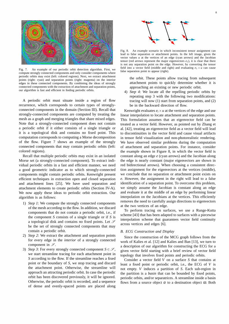
Fig. 7. An example of our periodic orbit detection algorithm. First, wecompute strongly connected components and only consider components whereperiodic orbits may exist (left: colored regions). Next, we extract attachmentpoints (right: cyan) and separation points (right: magenta) on the interioredges in these connected components. By combining the ideas of stronglyconnected components with the extraction of attachment and separation points,our algorithm is fast and efficient in finding periodic orbits.

A periodic orbit must situate inside a region of flowrecurrence, which corresponds to certain types of strongly-connected components in the domain (Section III). Recall thatstrongly-connected components are computed by treating themesh as a graph and merging triangles that share mixed edges.Note that a strongly-connected component does not containa periodic orbit if it either consists of a single triangle orit is a topological disk and contains no fixed point. Thiscomputation corresponds to computing a Morse decompositionof the flow. Figure 7 shows an example of the stronglyconnected components that may contain periodic orbits (left:colored regions).

Recall that multiple periodic orbits may exist in an isolatedMorse set (a strongly-connected component). To extract indi-vidual periodic orbits in a fast and efficient manner, we needa good geometric indicator as to which strongly-connectedcomponents might contain periodic orbits. Kenwright presentefficient techniques in extraction open and closed separationand attachment lines [25]. We have used separation andattachment elements to create periodic orbits (Section IV-A).We now apply these ideas to periodic orbit extraction. Ouralgorithm is as follows:

1) Step 1: We compute the strongly connected componentsof the mesh according to the flow. In addition, we discardcomponents that do not contain a periodic orbit, i.e., ifthe componentS consists of a single triangle or ifS isa topological disk and contains no fixed points. LetSbe the set of strongly connected components that maycontain a periodic orbit.

2) Step 2: We extract the attachment and separation pointsfor every edge in theinterior of a strongly connectedcomponent inS .

3) Step 3: For every strongly connected componentS∈S ,we start streamline tracing for each attachment point inSaccording to the flow. If the streamline reaches a fixedpoint or the boundary ofS, we stop tracing and discardthe attachment point. Otherwise, the streamline willapproach an attracting periodic orbit. In case the periodicorbit has been discovered previously, it will be ignored.Otherwise, the periodic orbit is recorded, and a sequenceof dense and evenly-spaced points are placed along

Fig. 8. An example scenario in which inconsistent tensor assignment canlead to false separation or attachment points. In the left image, given thevector valuesu at the vertices of an edge (cyan arrows) and the Jacobiantensor (red arrows represent the major eigenvectorse1), it is clear that thereis not any separation point on the edge. However, by converting the tensorfield into a vector field (middle and right) and evaluatinge1×u can causefalse separation point to appear (right).

the orbit. These points allow tracing from subsequentattachment points to quickly determine whether it isapproaching an existing or new periodic orbit.

4) Step 4: We locate all the repelling periodic orbits byrepeating step 3 with the following two modifications:tracing will now (1) start from separation points, and (2)be in the backward direction of flow.

Kenwright evaluatesei×u at the vertices of the edge and uselinear interpolation to locate attachment and separation points.This formulation assumes that an eigenvector field can betreated as a vector field. However, as pointed out by Zhang etal. [42], treating an eigenvector field as a vector field will leadto discontinuities in the vector field and cause visual artifactsin tensor field visualization and non-photorealistic rendering.We have observed similar problems during the computationof attachment and separation points. For instance, considerthe example shown in Figure 8, in which the vector field isconstant along an edgee (cyan arrows) and the Jacobian alongthe edge is nearly constant (major eigenvectors are shown inred bidirectional arrows). When choosing a consistent direc-tion assignment for the eigenvectors at the vertices (middle),we conclude that no separation or attachment point exists one. However, the assignment in the right will lead to a falseidentification of a separation point. To overcome this problem,we simply assume the Jacobian is constant along an edgeand evaluate it at the middle of an edge by performing linearinterpolation on the Jacobians at the vertices. This efficientlyremoves the need to carefully assign directions to eigenvectorsat the two vertices of an edge.

To perform tracing on surfaces, we use a Runge-Kuttascheme [43] that has been adapted to surfaces with a piecewiseinterpolation scheme that guarantees vector field continuityacross vertices and edges [6].

B. ECG Construction and Display

Since the construction of the MCG graph follows from thework of Kalies et al. [12] and Kalies and Ban [13], we turn toa description of our algorithm for constructing the ECG for agiven vector field starting with a brief review of vector fieldtopology that involves fixed points and periodic orbits.

Consider a vector fieldV on a surfaceS that contains atleast a fixed point or periodic orbit, i.e., the ECG ofV isnot empty.V induces a partition ofS. Each sub-region inthe partition is abasin that can be bounded by fixed points,periodic orbits, and/or separatrices. A streamline inside a basinflows from a source objectα to a destination objectω. Both

9

(a) (b) (c) (d) (e)

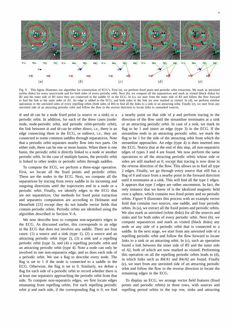
Fig. 9. This figure illustrates our algorithm for construction of ECG’s. First (a), we perform fixed point and periodic orbit extraction. We mark as unvisited(white disks) for every source/sink and for both sides of every periodic orbit. Next (b), we compute all the separatrices and mark as visited (black disks) forR2 and the outer side ofR3 since they are connected to the saddleS1 in the ECG. In (c), we start from the inner side ofR3 and follow the flow forwardto find the link to the outer sider ofA2. An edge is added to the ECG, and both sides in the link are now marked as visited. In (d), we perform similiaroperations to the unvisited sides of every repelling orbits (both sides ofR4) to find all the links to a sink or an attracting orbit. Finally (e), we start from anyunvisited side of an attracting periodic orbit and follow the flow in the reverse direction to locate links to unmarked sources.

α and ω can be a node fixed point (a source or a sink) or aperiodic orbit. In addition, for each of the three cases (node-node, node-periodic orbit, and periodic orbit-periodic orbit),the link betweenα andω can be either direct, i.e., there is anedge connecting them in the ECG, or indirect, i.e., they areconnected to some common saddles through separatrices. Notethat a periodic orbit separates nearby flow into two parts. Oneither side, there can be one or more basins. When there is onebasin, the periodic orbit is directly linked to a node or anotherperiodic orbit. In the case of multiple basins, the periodic orbitis linked to other nodes or periodic orbits through saddles.

To compute the ECG, we perform a three-stage operation.First, we locate all the fixed points and periodic orbits.These are the nodes in the ECG. Next, we compute all theseparatrices by tracing from every saddle in its incoming andoutgoing directions until the trajectories end in a node or aperiodic orbit. Finally, we identify edges in the ECG thatare not separatrices. Our methods for fixed point extractionand separatrix computation are according to Helmann andHesselink [23] except they do not handle vector fields thatcontain periodic orbits. Periodic orbits are identified using thealgorithm described in Section V-A.

We now describe how to compute non-separatrix edges inthe ECG. As discussed earlier, this corresponds to an edgein the ECG that does not involves any saddle. There are fourcases: (1) a source and a sink (type1), (2) a source and anattracting periodic orbit (type2), (3) a sink and a repellingperiodic orbit (type3), and (4) a repelling periodic orbit andan attracting periodic orbit (type4). Note a node can only beinvolved in one non-separatrix edge, and so does each side ofa periodic orbit. We use a flag to describe every node. Theflag is set to1 if the node is connected to a saddle in theECG. Otherwise, the flag is set to0. Similarly, we define aflag for each side of a periodic orbit to record whether there isat least one separatrix approaching the periodic orbit from thatside. To compute non-separatrix edges, we first locate edgesemanating from repelling orbits. For each repelling periodicorbit γ and each side, if the corresponding flag is0, we find

a nearby point on that side ofγ and perform tracing in thedirection of the flow until the streamline terminates at a sinkor an attracting periodic orbit. In case of a sink, we mark itsflag to be1 and insert an edge (type3) in the ECG. If thestreamline ends in an attracting periodic orbit, we mark theflag to be1 for the side of the attracting orbit from which thestreamline approaches. An edge (type 4) is then inserted intothe ECG. Notice that at the end of this step, all non-separatrixedges of types3 and4 are found. We now perform the sameoperations to all the attracting periodic orbits whose side orsides are still marked as0, except that tracing is now done inthe reverse direction of the flow. This allows us to find all type2 edges. Finally, we go through every source that still has aflag of 0 and trace from a nearby point in the forward directionuntil it terminates at a sink. This will find all the type1 edges.It appears that type1 edges are rather uncommon. In fact, theonly instance that we know of is the idealized magnetic fieldover a sphere, which contains two fixed points and no periodicorbits. Figure 9 illustrates this process with an example vectorfield that contains two sources, one saddle, and four periodicorbits. In (a), we extract all the fixed points and periodic orbits.We also mark as unvisited (white disks) for all the sources andsinks and for both sides of every periodic orbit. Next (b), wecompute separatrices and mark as visited (black disks) anynode or any side of a periodic orbit that is connected to asaddle. In the next stage, we start from any unvisited side of arepelling periodic orbit and follow the flow forward to locatelinks to a sink or an attracting orbit. In (c), such an operationfound a link between the inner side ofR3 and the outer sideof A2, both of which are now marked as visited. Performingthis operation on all the repelling periodic orbits leads to (d),in which links such asR4/A1 and R4/A2 are found. Finally(e), we start from any unvisited side of an attracting periodicorbit and follow the flow in the reverse direction to locate theremaining edges in the ECG.

To display an ECG, we arrange vector field features (fixedpoints and periodic orbits) in three rows, with sources andrepelling period orbits in the top row, sinks and attracting

10

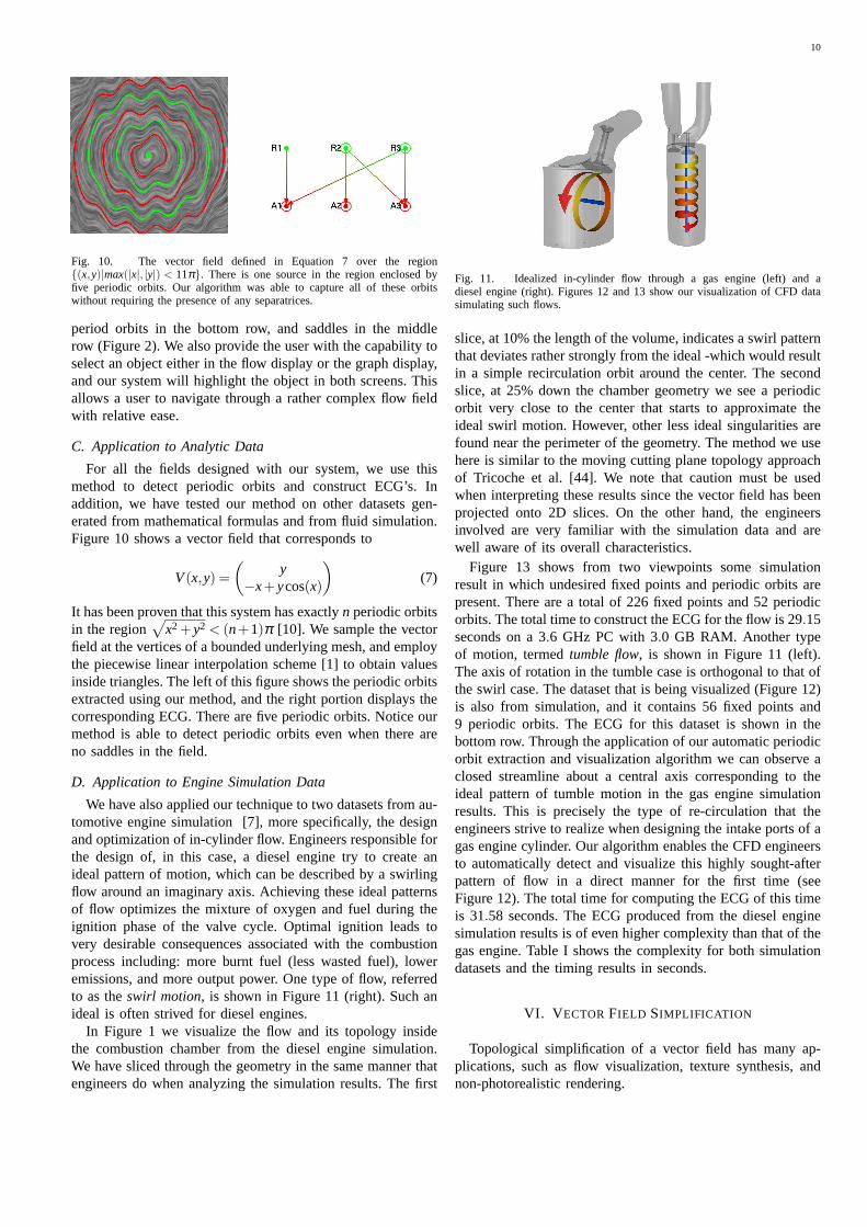
Fig. 10. The vector field defined in Equation 7 over the region{(x,y)|max(|x|, |y|) < 11π}. There is one source in the region enclosed byfive periodic orbits. Our algorithm was able to capture all of these orbitswithout requiring the presence of any separatrices.

period orbits in the bottom row, and saddles in the middlerow (Figure 2). We also provide the user with the capability toselect an object either in the flow display or the graph display,and our system will highlight the object in both screens. Thisallows a user to navigate through a rather complex flow fieldwith relative ease.

C. Application to Analytic Data

For all the fields designed with our system, we use thismethod to detect periodic orbits and construct ECG’s. Inaddition, we have tested our method on other datasets gen-erated from mathematical formulas and from fluid simulation.Figure 10 shows a vector field that corresponds to

V(x,y) =(

y−x+ycos(x)

)(7)

It has been proven that this system has exactlyn periodic orbitsin the region

√x2 +y2 < (n+1)π [10]. We sample the vector

field at the vertices of a bounded underlying mesh, and employthe piecewise linear interpolation scheme [1] to obtain valuesinside triangles. The left of this figure shows the periodic orbitsextracted using our method, and the right portion displays thecorresponding ECG. There are five periodic orbits. Notice ourmethod is able to detect periodic orbits even when there areno saddles in the field.

D. Application to Engine Simulation Data

We have also applied our technique to two datasets from au-tomotive engine simulation [7], more specifically, the designand optimization of in-cylinder flow. Engineers responsible forthe design of, in this case, a diesel engine try to create anideal pattern of motion, which can be described by a swirlingflow around an imaginary axis. Achieving these ideal patternsof flow optimizes the mixture of oxygen and fuel during theignition phase of the valve cycle. Optimal ignition leads tovery desirable consequences associated with the combustionprocess including: more burnt fuel (less wasted fuel), loweremissions, and more output power. One type of flow, referredto as theswirl motion, is shown in Figure 11 (right). Such anideal is often strived for diesel engines.

In Figure 1 we visualize the flow and its topology insidethe combustion chamber from the diesel engine simulation.We have sliced through the geometry in the same manner thatengineers do when analyzing the simulation results. The first

Fig. 11. Idealized in-cylinder flow through a gas engine (left) and adiesel engine (right). Figures 12 and 13 show our visualization of CFD datasimulating such flows.

slice, at10%the length of the volume, indicates a swirl patternthat deviates rather strongly from the ideal -which would resultin a simple recirculation orbit around the center. The secondslice, at25% down the chamber geometry we see a periodicorbit very close to the center that starts to approximate theideal swirl motion. However, other less ideal singularities arefound near the perimeter of the geometry. The method we usehere is similar to the moving cutting plane topology approachof Tricoche et al. [44]. We note that caution must be usedwhen interpreting these results since the vector field has beenprojected onto 2D slices. On the other hand, the engineersinvolved are very familiar with the simulation data and arewell aware of its overall characteristics.

Figure 13 shows from two viewpoints some simulationresult in which undesired fixed points and periodic orbits arepresent. There are a total of226 fixed points and52 periodicorbits. The total time to construct the ECG for the flow is29.15seconds on a3.6 GHz PC with3.0 GB RAM. Another typeof motion, termedtumble flow, is shown in Figure 11 (left).The axis of rotation in the tumble case is orthogonal to that ofthe swirl case. The dataset that is being visualized (Figure 12)is also from simulation, and it contains56 fixed points and9 periodic orbits. The ECG for this dataset is shown in thebottom row. Through the application of our automatic periodicorbit extraction and visualization algorithm we can observe aclosed streamline about a central axis corresponding to theideal pattern of tumble motion in the gas engine simulationresults. This is precisely the type of re-circulation that theengineers strive to realize when designing the intake ports of agas engine cylinder. Our algorithm enables the CFD engineersto automatically detect and visualize this highly sought-afterpattern of flow in a direct manner for the first time (seeFigure 12). The total time for computing the ECG of this timeis 31.58 seconds. The ECG produced from the diesel enginesimulation results is of even higher complexity than that of thegas engine. Table I shows the complexity for both simulationdatasets and the timing results in seconds.

VI. V ECTORFIELD SIMPLIFICATION

Topological simplification of a vector field has many ap-plications, such as flow visualization, texture synthesis, andnon-photorealistic rendering.

11

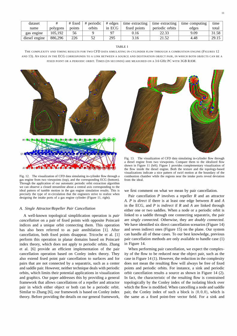
dataset # # fixed # periodic # edges time extracting time extracting time computing timename polygons points orbits in ECG fixed points periodic orbits edges total

gas engine 105,192 56 9 97 0.16 22.33 9.09 31.58diesel engine 886,296 226 52 295 3.16 21.52 4.48 29.15

TABLE I

THE COMPLEXITY AND TIMING RESULTS FOR TWOCFD DATA SIMULATING IN -CYLINDER FLOW THROUGH A COMBUSTION ENGINE(FIGURES12

AND 13). AN EDGE IN THE ECG CORRESPONDS TO A LINK BETWEEN A SOURCE AND DESTINATION OBJECT PAIR, IN WHICH BOTH OBJECTS CAN BE A

FIXED POINT OR A PERIODIC ORBIT. TIMES (IN SECONDS) ARE MEASURED ON A3.6 GHZ PC WITH 3GB RAM.

Fig. 12. The visualization of CFD data simulating in-cylinder flow through agas engine from two viewpoints (top), and the corresponding ECG (bottom).Through the application of our automatic periodic orbit extraction algorithmwe can observe a closed streamline about a central axis corresponding to theideal pattern of tumble motion in the gas engine simulation results. This isprecisely the type of re-circulation that the engineers strive to realize whendesigning the intake ports of a gas engine cylinder (Figure 11, right).

A. Single Attractor/Repeller Pair Cancellation

A well-known topological simplification operation ispaircancellationon a pair of fixed points with opposite Poincareindices and a unique orbit connecting them. This operationhas also been referred to as pair annihilation [1]. Aftercancellation, both fixed points disappear. Tricoche et al. [1]perform this operation in planar domains based on Poincareindex theory, which does not apply to periodic orbits. Zhanget al. [6] provide an efficient implementation of the paircancellation operation based on Conley index theory. Theyalso extend fixed point pair cancellation to surfaces and forpairs that are not connected by a separatrix, such as a centerand saddle pair. However, neither technique deals with periodicorbits, which limits their potential applications in visualizationand graphics. Our paper addresses this by providing a generalframework that allows cancellations of a repeller and attractorpair in which either object or both can be a periodic orbit.Similar to Zhang [6], our framework is based on Conley indextheory. Before providing the details on our general framework,

Fig. 13. The visualization of CFD data simulating in-cylinder flow througha diesel engine from two viewpoints. Compare them to the idealized flowshown in Figure 11 (left). Figure 1 provides complementary visualization ofthe flow inside the diesel engine. Both the texture and the topology-basedvisualizations indicate a nice pattern of swirl motion at the boundary of thecombustion chamber while the regions near the intake ports reveal deviationfrom the ideal.

we first comment on what we mean by pair cancellation.Pair cancellationP involves a repellerR and an attractor

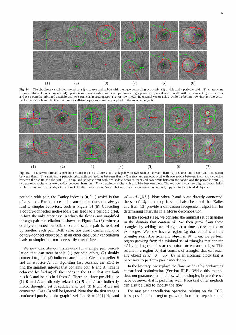
A. P is direct if there is at least one edge betweenR and Ain the ECG, andP is indirect if R and A are linked througheither one or two saddles. When a node or a periodic orbit islinked to a saddle through one connecting separatrix, the pairare singly connected. Otherwise, they aredoubly connected.We have identified six direct cancellation scenarios (Figure 14)and seven indirect ones (Figure 15) on the plane. Our systemcan handle all of these cases. To our best knowledge, previouspair cancellation methods are only available to handle case (1)in Figure 14.

When performing pair cancellation, we expect the complex-ity of the flow to be reduced near the object pair, such as thecase in Figure 14 (1). However, the reduction in the complexitydoes not mean the resulting flow will always be free of fixedpoints and periodic orbits. For instance, a sink and periodicorbit cancellation results a source as shown in Figure 14 (2).In fact, the characteristic of the resulting flow is constrainedtopologically by the Conley index of the isolating block overwhich the flow is modified. When cancelling a node and saddlepair, the Conley index of such a block is(0,0,0), which isthe same as a fixed point-free vector field. For a sink and

12

(1) (2) (3) (4) (5) (6)Fig. 14. The six direct cancelation scenarios: (1) a source and saddle with a unique connecting separatrix, (2) a sink and a periodic orbit, (3) an attractingperiodic orbit and a repelling one, (4) a periodic orbit and a saddle with a unique connecting separatrix, (5) a sink and a saddle with two connecting separatrices,and (6) a periodic orbit and a saddle with two connecting separatrices. The top row shows the original vector fields, while the bottom row displays the vectorfield after cancellation. Notice that our cancellation operations are only applied to the intended objects.

(1) (2) (3) (4) (5) (6) (7)Fig. 15. The seven indirect cancellation scenarios: (1) a source and a sink pair with two saddles between them, (2) a source and a sink with one saddlebetween them, (3) a sink and a periodic orbit with two saddles between them, (4) a sink and periodic orbit with one saddle between them and two orbitsbetween the saddle and the sink, (5) a sink and periodic orbit with one saddle between them and two orbits between the saddle and the periodic orbit, (6)two periodic orbits with two saddles between them, and (7) two periodic orbits with a saddle between them. The top row shows the original vector fields,while the bottom row displays the vector field after cancellation. Notice that our cancellation operations are only applied to the intended objects.

periodic orbit pair, the Conley index is(0,0,1) which is thatof a source. Furthermore, pair cancellation does not alwayslead to simpler behaviors, such as Figure 14 (5). Cancellinga doubly-connected node-saddle pair leads to a periodic orbit.In fact, the only other case in which the flow is not simplifiedthrough pair cancellation is shown in Figure 14 (6), where adoubly-connected periodic orbit and saddle pair is replacedby another such pair. Both cases are direct cancellations ofdoubly-connect object pair. In all other cases, pair cancellationleads to simpler but not necessarily trivial flow.

We now describe our framework for a single pair cancel-lation that can now handle (1) periodic orbits, (2) doublyconnections, and (3) indirect cancellation. Given a repellerRand an attractorA, our algorithm first searches the ECG tofind the smallest interval that contains bothR and A. This isachieved by finding all the nodes in the ECG that can bothreachA and be reached fromR. There are three possibilities:(1) R and A are directly related, (2)R and A are indirectlylinked through a set of saddlesSi ’s, and (3)R and A are notconnected. Case (3) will be ignored. Note that the first stage isconducted purely on the graph level. LetR = {R}⋃{Si} and

A = {A}⋃{Si}. Note whenR and A are directly connected,the set of{Si} is empty. It should also be noted that Kaliesand Ban [13] provide a dimension independent algorithm fordetermining intervals in a Morse decomposition.

In the second stage, we consider the minimal set of trianglesin the domain that containR. We then grow from thesetriangles by adding one triangle at a time across mixed orexit edges. We now have a regionUR that contains all thetriangles reachable from any object inR. Then, we performregion growing from the minimal set of triangles that containA by adding triangles across mixed or entrance edges. Thisresults in a regionUA that consists of triangles that can reachany object inA . U = UR

⋂UA is an isolating block that is

necessary to perform pair cancellation.

In the last step, we replace the flow insideU by performingconstrained optimization (Section III-E). While this methoddoes not guarantee that the flow will be simpler, in practice wehave observed that it performs well. Note that other methodscan also be used to modify the flow.

For any pair cancellation operation relying on the ECG,it is possible that region growing from the repellers and

13

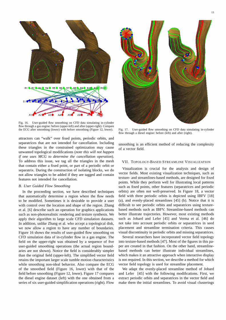
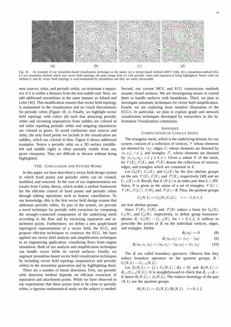
Fig. 16. User-guided flow smoothing on CFD data simulating in-cylinderflow through a gas engine: before (upper-left) and after (upper-right). Comparethe ECG after smoothing (lower) with before smoothing (Figure 12, lower).

attractors can “walk” over fixed points, periodic orbits, andseparatrices that are not intended for cancellation. Includingthese triangles in the constrained optimization may causeunwanted topological modifications (note this will not happenif one uses MCG to determine the cancellation operation).To address this issue, we tag all the triangles in the meshthat contain either a fixed point, or part of a periodic orbit orseparatrix. During the construction of isolating blocks, we donot allow triangles to be added if they are tagged and containfeatures not intended for cancellation.

B. User Guided Flow Smoothing

In the proceeding section, we have described techniquesthat automatically determine a region where the flow needsto be modified. Sometimes it is desirable to provide a userwith control over the location and shape of the region. Zhanget al. [6] describe such an operation for graphics applicationssuch as non-photorealistic rendering and texture synthesis. Weapply their algorithm to large scale CFD simulation datasets.In addition, unlike Zhang et al. who accept a topological disk,we now allow a region to have any number of boundaries.Figure 16 shows the results of user-guided flow smoothing onCFD simulation data of in-cylinder flow in a gas engine. Thefield on the upper-right was obtained by a sequence of fiveuser-guided smoothing operations (the actual region bound-aries are not shown). Notice the field is considerably simplerthan the original field (upper-left). The simplified vector fieldretains the important larger scale tumble motion characteristicswhile smoothing non-ideal behavior. Also compare the ECGof the smoothed field (Figure 16, lower) with that of thefield before smoothing (Figure 12, lower). Figure 17 comparesthe diesel engine dataset (left) with the one obtained from aseries of six user-guided simplification operations (right). Flow

Fig. 17. User-guided flow smoothing on CFD data simulating in-cylinderflow through a diesel engine: before (left) and after (right).

smoothing is an efficient method of reducing the complexityof a vector field.

VII. T OPOLOGY-BASED STREAMLINE V ISUALIZATION

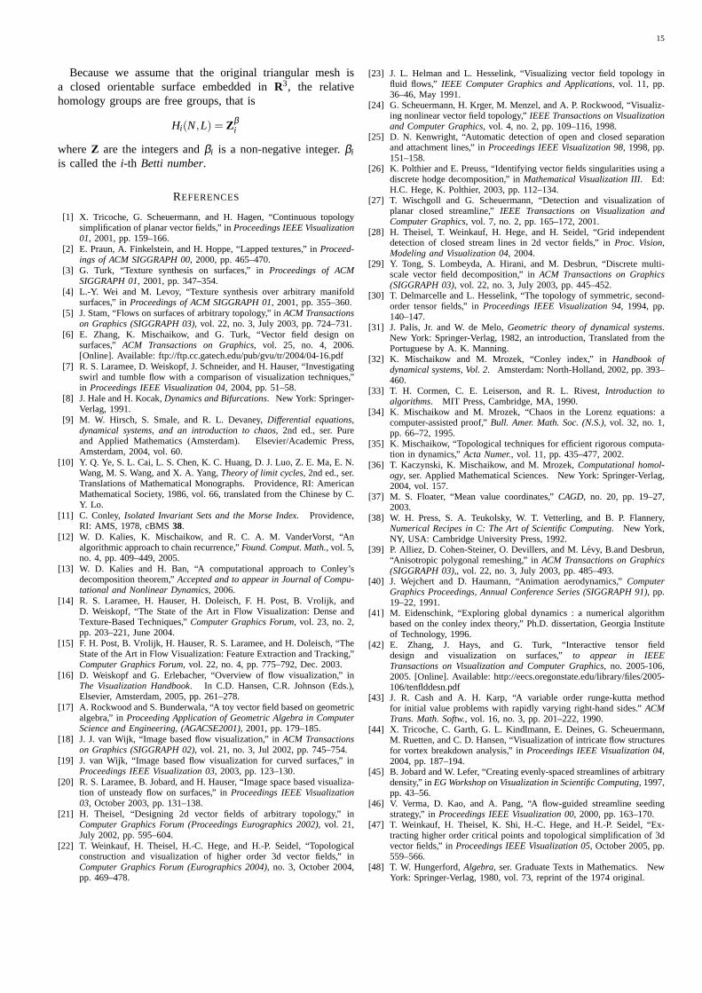
Visualization is crucial for the analysis and design ofvector fields. Most existing visualization techniques, such astexture- and streamlines-based methods, are designed for fixedpoints. While they perform well for illustrating local patternssuch as fixed points, other features (separatrices and periodicorbits) are often not well-preserved. In Figure 18, a vectorfield with three periodic orbits is depicted using IBFV [18](a), and evenly-placed streamlines [45] (b). Notice that it isdifficult to see periodic orbits and separatrices using texture-based methods such as IBFV. Streamline-based methods canbetter illustrate trajectories. However, most existing methodssuch as Jobard and Lefer [45] and Verma et al. [46] donot take into account periodic orbits or separatrices in seedplacement and streamline termination criteria. This causesvisual discontinuity in periodic orbits and missing separatrices.

Several researchers have incorporated vector field topologyinto texture-based methods [47]. Most of the figures in this pa-per are created in that fashion. On the other hand, streamline-based methods can better illustrate individual streamlines,which makes it an attractive approach when interactive displayis not required. In this section, we describe a method for whichvector field topology is used for streamline placement.

We adapt the evenly-placed streamline method of Jobardand Lefer [45] with the following modifications. First, weextract periodic orbits and separatrices in the vector field andmake them the initial streamlines. To avoid visual clusterings

14

(a) (b) (c) (d)Fig. 18. An example of our streamline-based visualization technique on the plane: (a) a texture-based method (IBFV [18]), (b) a streamline-method [45],(c) our streamline method which uses vector field topology, (d) same image from (c) with periodic orbits and separatrices being highlighted. Notice with ourmethod (c and d), vector field topology is well-maintained by streamlines and they are easily discernable.

near sources, sinks, and periodic orbits, we terminate a separa-trix if it is within a distance from the non-saddle end. Next, weadd additional streamlines in the same manner as Jobard andLefer [45]. This modification ensures that vector field topologyis maintained in the visualization and no visual discontinuityfor periodic orbits (Figure 18, c). Finally, we highlight vectorfield topology with colors (d) such that attracting periodicorbits and incoming separatrices from saddles are colored inred while repelling periodic orbits and outgoing separatricesare colored in green. To avoid confusions near sources andsinks, the only fixed points we include in the visualization aresaddles, which are colored in blue. Figure 6 shows additionalexamples. Notice a periodic orbit on a 3D surface (middle-left and middle right) is often partially visible from anygiven viewpoint. They are difficult to discern without beinghighlighted.

VIII. C ONCLUSION AND FUTURE WORK

In this paper, we have described a vector field design systemin which fixed points and periodic orbits can be created,modified, and removed. At the core of our implementation areresults from Conley theory, which enable a unified frameworkfor the efficient control of fixed points and periodic orbitsthrough editing operations such as feature cancellation. Toour knowledge, this is the first vector field design system thataddresses periodic orbits. As part of the system, we providea novel technique for periodic orbit extraction by computingthe strongly-connected components of the underlying meshaccording to the flow and by extracting separation and at-tachment points. Furthermore, we define a new graph-basedtopological representation of a vector field, the ECG, andpropose efficient techniques to construct the ECG. We haveapplied our vector field analysis and simplification techniquesto an engineering application: visualizing flows from enginesimulation. Both of our analysis and simplification techniquescan handle vector fields on curved surfaces. Finally, weaugment streamline-based vector field visualization techniquesby including vector field topology (separatrices and periodicorbits) in the streamline generation and by highlighting them.

There are a number of future directions. First, our periodicorbit detection method depends on efficient extraction ofseparation and attachment points. While we have observed inour experiments that these points tend to be close to periodicorbits, a rigorous mathematical study on the subject is needed.

Second, our current MCG and ECG construction methodsassume closed surfaces. We are investigating means to extendthem to handle surfaces with boundaries. Third, we plan toinvestigate automatic techniques for vector field simplification.Fourth, we are exploring more intuitive illustration of theECG’s. In particular, we plan to explore graph and networkvisualization techniques developed by researchers in the In-formation Visualization community.

APPENDIX

COMPUTATION OF CONLEY INDEX

The triangular mesh, which is the underlying domain for oursystem, consists of a collection of vertices,V whose elementsare denoted by〈vi〉, edgesE , whose elements are denoted by〈vi ,v j〉, i 6= j, and trianglesT , whose elements are denotedby 〈vi ,v j ,vk〉, i 6= j 6= k 6= i. Given a subsetX of the mesh,let V (X), E (X), andT (X) denote the collections of vertices,edges, and triangles which are contained inX.

Let C0(X), C1(X), and C2(X) be the free abelian groupson the setsV (X), E (X), andT (X), respectively [48] and setC−1(X) = 0. Recall, that if(N,L) is an index pair thenL⊂ ∂N.Since,N is given as the union of a set of triangles,V (L) ⊂V (N), E (L)⊂ E (N), andT (L) = /0. Thus, the quotient groups

Ci(N,L) := Ci(N)/Ci(L), i =−1,0,1,2

are free abelian groups.SinceV (N), E (N), and T (N) induce a basis forC0(N),

C1(N), and C2(N), respectively, to define group homomor-phisms ∂i : Ci(N) → Ci−1(N), for i = 0,1,2, it suffices toprescribe the action of∂i on the individual vertices, edges,and triangles. Define

∂0〈v0〉 := 0 (8)

∂1〈v0,v1〉 := 〈v1〉−〈v0〉 (9)

∂2〈v0,v1,v2〉 := 〈v0,v1〉−〈v0,v2〉+ 〈v1,v2〉 (10)

The ∂i are calledboundary operators. Observe that theyinduce boundary operators on the quotient groups,∂i :Ci(N,L)→Ci−1(N,L).

Let Zi(N,L) := {x ∈ Ci(N,L) | ∂ix = 0} and Bi(N,L) :=∂i+1(Ci+1(N,L)). It is straightforward to check that∂i−1◦∂i =0, henceBi(N,L)⊂Zi(N,L). Therelative homologyof the pair(N,L) are the quotient groups

Hi(N,L) := Zi(N,L)/Bi(N,L) i = 0,1,2.

15

Because we assume that the original triangular mesh isa closed orientable surface embedded inR3, the relativehomology groups are free groups, that is

Hi(N,L) = Zβi

whereZ are the integers andβi is a non-negative integer.βi

is called thei-th Betti number.

REFERENCES

[1] X. Tricoche, G. Scheuermann, and H. Hagen, “Continuous topologysimplification of planar vector fields,” inProceedings IEEE Visualization01, 2001, pp. 159–166.

[2] E. Praun, A. Finkelstein, and H. Hoppe, “Lapped textures,” inProceed-ings of ACM SIGGRAPH 00, 2000, pp. 465–470.

[3] G. Turk, “Texture synthesis on surfaces,” inProceedings of ACMSIGGRAPH 01, 2001, pp. 347–354.

[4] L.-Y. Wei and M. Levoy, “Texture synthesis over arbitrary manifoldsurfaces,” inProceedings of ACM SIGGRAPH 01, 2001, pp. 355–360.

[5] J. Stam, “Flows on surfaces of arbitrary topology,” inACM Transactionson Graphics (SIGGRAPH 03), vol. 22, no. 3, July 2003, pp. 724–731.

[6] E. Zhang, K. Mischaikow, and G. Turk, “Vector field design onsurfaces,” ACM Transactions on Graphics, vol. 25, no. 4, 2006.[Online]. Available: ftp://ftp.cc.gatech.edu/pub/gvu/tr/2004/04-16.pdf

[7] R. S. Laramee, D. Weiskopf, J. Schneider, and H. Hauser, “Investigatingswirl and tumble flow with a comparison of visualization techniques,”in Proceedings IEEE Visualization 04, 2004, pp. 51–58.

[8] J. Hale and H. Kocak,Dynamics and Bifurcations. New York: Springer-Verlag, 1991.

[9] M. W. Hirsch, S. Smale, and R. L. Devaney,Differential equations,dynamical systems, and an introduction to chaos, 2nd ed., ser. Pureand Applied Mathematics (Amsterdam). Elsevier/Academic Press,Amsterdam, 2004, vol. 60.

[10] Y. Q. Ye, S. L. Cai, L. S. Chen, K. C. Huang, D. J. Luo, Z. E. Ma, E. N.Wang, M. S. Wang, and X. A. Yang,Theory of limit cycles, 2nd ed., ser.Translations of Mathematical Monographs. Providence, RI: AmericanMathematical Society, 1986, vol. 66, translated from the Chinese by C.Y. Lo.

[11] C. Conley,Isolated Invariant Sets and the Morse Index. Providence,RI: AMS, 1978, cBMS38.

[12] W. D. Kalies, K. Mischaikow, and R. C. A. M. VanderVorst, “Analgorithmic approach to chain recurrence,”Found. Comput. Math., vol. 5,no. 4, pp. 409–449, 2005.

[13] W. D. Kalies and H. Ban, “A computational approach to Conley’sdecomposition theorem,”Accepted and to appear in Journal of Compu-tational and Nonlinear Dynamics, 2006.

[14] R. S. Laramee, H. Hauser, H. Doleisch, F. H. Post, B. Vrolijk, andD. Weiskopf, “The State of the Art in Flow Visualization: Dense andTexture-Based Techniques,”Computer Graphics Forum, vol. 23, no. 2,pp. 203–221, June 2004.

[15] F. H. Post, B. Vrolijk, H. Hauser, R. S. Laramee, and H. Doleisch, “TheState of the Art in Flow Visualization: Feature Extraction and Tracking,”Computer Graphics Forum, vol. 22, no. 4, pp. 775–792, Dec. 2003.

[16] D. Weiskopf and G. Erlebacher, “Overview of flow visualization,” inThe Visualization Handbook. In C.D. Hansen, C.R. Johnson (Eds.),Elsevier, Amsterdam, 2005, pp. 261–278.

[17] A. Rockwood and S. Bunderwala, “A toy vector field based on geometricalgebra,” inProceeding Application of Geometric Algebra in ComputerScience and Engineering, (AGACSE2001), 2001, pp. 179–185.

[18] J. J. van Wijk, “Image based flow visualization,” inACM Transactionson Graphics (SIGGRAPH 02), vol. 21, no. 3, Jul 2002, pp. 745–754.

[19] J. van Wijk, “Image based flow visualization for curved surfaces,” inProceedings IEEE Visualization 03, 2003, pp. 123–130.

[20] R. S. Laramee, B. Jobard, and H. Hauser, “Image space based visualiza-tion of unsteady flow on surfaces,” inProceedings IEEE Visualization03, October 2003, pp. 131–138.

[21] H. Theisel, “Designing 2d vector fields of arbitrary topology,” inComputer Graphics Forum (Proceedings Eurographics 2002), vol. 21,July 2002, pp. 595–604.

[22] T. Weinkauf, H. Theisel, H.-C. Hege, and H.-P. Seidel, “Topologicalconstruction and visualization of higher order 3d vector fields,” inComputer Graphics Forum (Eurographics 2004), no. 3, October 2004,pp. 469–478.

[23] J. L. Helman and L. Hesselink, “Visualizing vector field topology influid flows,” IEEE Computer Graphics and Applications, vol. 11, pp.36–46, May 1991.

[24] G. Scheuermann, H. Krger, M. Menzel, and A. P. Rockwood, “Visualiz-ing nonlinear vector field topology,”IEEE Transactions on Visualizationand Computer Graphics, vol. 4, no. 2, pp. 109–116, 1998.

[25] D. N. Kenwright, “Automatic detection of open and closed separationand attachment lines,” inProceedings IEEE Visualization 98, 1998, pp.151–158.

[26] K. Polthier and E. Preuss, “Identifying vector fields singularities using adiscrete hodge decomposition,” inMathematical Visualization III. Ed:H.C. Hege, K. Polthier, 2003, pp. 112–134.

[27] T. Wischgoll and G. Scheuermann, “Detection and visualization ofplanar closed streamline,”IEEE Transactions on Visualization andComputer Graphics, vol. 7, no. 2, pp. 165–172, 2001.

[28] H. Theisel, T. Weinkauf, H. Hege, and H. Seidel, “Grid independentdetection of closed stream lines in 2d vector fields,” inProc. Vision,Modeling and Visualization 04, 2004.

[29] Y. Tong, S. Lombeyda, A. Hirani, and M. Desbrun, “Discrete multi-scale vector field decomposition,” inACM Transactions on Graphics(SIGGRAPH 03), vol. 22, no. 3, July 2003, pp. 445–452.

[30] T. Delmarcelle and L. Hesselink, “The topology of symmetric, second-order tensor fields,” inProceedings IEEE Visualization 94, 1994, pp.140–147.

[31] J. Palis, Jr. and W. de Melo,Geometric theory of dynamical systems.New York: Springer-Verlag, 1982, an introduction, Translated from thePortuguese by A. K. Manning.

[32] K. Mischaikow and M. Mrozek, “Conley index,” inHandbook ofdynamical systems, Vol. 2. Amsterdam: North-Holland, 2002, pp. 393–460.

[33] T. H. Cormen, C. E. Leiserson, and R. L. Rivest,Introduction toalgorithms. MIT Press, Cambridge, MA, 1990.

[34] K. Mischaikow and M. Mrozek, “Chaos in the Lorenz equations: acomputer-assisted proof,”Bull. Amer. Math. Soc. (N.S.), vol. 32, no. 1,pp. 66–72, 1995.

[35] K. Mischaikow, “Topological techniques for efficient rigorous computa-tion in dynamics,”Acta Numer., vol. 11, pp. 435–477, 2002.

[36] T. Kaczynski, K. Mischaikow, and M. Mrozek,Computational homol-ogy, ser. Applied Mathematical Sciences. New York: Springer-Verlag,2004, vol. 157.

[37] M. S. Floater, “Mean value coordinates,”CAGD, no. 20, pp. 19–27,2003.

[38] W. H. Press, S. A. Teukolsky, W. T. Vetterling, and B. P. Flannery,Numerical Recipes in C: The Art of Scientific Computing. New York,NY, USA: Cambridge University Press, 1992.

[39] P. Alliez, D. Cohen-Steiner, O. Devillers, and M. Levy, B.and Desbrun,“Anisotropic polygonal remeshing,” inACM Transactions on Graphics(SIGGRAPH 03),, vol. 22, no. 3, July 2003, pp. 485–493.

[40] J. Wejchert and D. Haumann, “Animation aerodynamics,”ComputerGraphics Proceedings, Annual Conference Series (SIGGRAPH 91), pp.19–22, 1991.

[41] M. Eidenschink, “Exploring global dynamics : a numerical algorithmbased on the conley index theory,” Ph.D. dissertation, Georgia Instituteof Technology, 1996.

[42] E. Zhang, J. Hays, and G. Turk, “Interactive tensor fielddesign and visualization on surfaces,”to appear in IEEETransactions on Visualization and Computer Graphics, no. 2005-106,2005. [Online]. Available: http://eecs.oregonstate.edu/library/files/2005-106/tenflddesn.pdf

[43] J. R. Cash and A. H. Karp, “A variable order runge-kutta methodfor initial value problems with rapidly varying right-hand sides.”ACMTrans. Math. Softw., vol. 16, no. 3, pp. 201–222, 1990.

[44] X. Tricoche, C. Garth, G. L. Kindlmann, E. Deines, G. Scheuermann,M. Ruetten, and C. D. Hansen, “Visualization of intricate flow structuresfor vortex breakdown analysis,” inProceedings IEEE Visualization 04,2004, pp. 187–194.

[45] B. Jobard and W. Lefer, “Creating evenly-spaced streamlines of arbitrarydensity,” inEG Workshop on Visualization in Scientific Computing, 1997,pp. 43–56.

[46] V. Verma, D. Kao, and A. Pang, “A flow-guided streamline seedingstrategy,” inProceedings IEEE Visualization 00, 2000, pp. 163–170.

[47] T. Weinkauf, H. Theisel, K. Shi, H.-C. Hege, and H.-P. Seidel, “Ex-tracting higher order critical points and topological simplification of 3dvector fields,” inProceedings IEEE Visualization 05, October 2005, pp.559–566.

[48] T. W. Hungerford,Algebra, ser. Graduate Texts in Mathematics. NewYork: Springer-Verlag, 1980, vol. 73, reprint of the 1974 original.