Vegetation Products from L-Band measurements

Arnaud Mialon

13/09/2018

arnaud.mialon@cesbio.cnes.fr

http://www.cesbio.ups-tlse.fr/SMOS_blog/

http://www.catds.fr/

TeamYann Kerr, Philippe Richaume, François Cabot, Nemesio Rodriguez, Ahmad Al Bitar, Christophe Suere, Eric Anterrieu, Ali Khazaal, Arnaud Mialon.Level 1 TB : algo, calibration.ESA level 2 : Soil Moisture / VOD retrieval algorithm from SMOSCATDS level 3 and 4

http://www.esa.int/Our_Activities/Observing_the_Earth/SMOS

Objectives

Present VOD (Vegetation Optical Depth) derived from SMOS

Read SMOS Data using Matlab

SMOS (Soil Moisture and Ocean Salinity)

• ESA Earth Explorer Mission

• Launched in Nov.2009, data available since May 2010

• Passive microwave L-Band ( = 21 cm, f=1.4 GHz)

• Main Objectives Surface Soil Moisture (m3 of water/m3 of soil)Sea Surface Salinity

• Resolution Orbit ~polar, Sun synchronous

Ascending orbits = 6am solar local timeDescending orbits = 6 pm solar local time

Level 2 : 15km Soil moiture and VegetationSpatial : covers the Earth Surface in ~3 days

Passive microwave L-Band ( = 21 cm, f=1.4 GHz)

• Passive measure the Emission of the Earth Surface

• Microwave Brightness Temperatures TBat Horizontal and Vertical Polarisation

SMOS BT Y polarization

SMOS BT X polarization

∆ Modeled BT

‘L-MEB’ model: L-band Microwave Emission of the Biosphere

Simple radiative transfer (RT) model for a soil-vegetation system

References: Wigneron et al., RSE, 2007 ; Kerr et al. 2012

6

From SMOS TB observations to soil / vegetation at Surface level

TB,tot(P,θ) = esTsγ + (1 – ω) (1 - γ)Tv + (1 – ω) (1 - γ)Tv (1 - es) γ + TB,skyγ2 (1 - es)

es soil emissivity; linked to soil moisture through dielectric constant (P,θ)Ts physical temperature of soilTv physical temperature of vegetationω single scattering albedo of vegetation (omega) (P,θ)γ canopy transmissivity; linked to vegetation optical depth τ (tau) (P,θ)TBsky sky brightness temperature (P,θ)

P polarisation (H or V)θ incidence angle

1. soil 2. vegetation 3. vegetation-soil 4. sky

7

L-MEB algorithm

1. soil2. vegetation

3. vegetation-soil

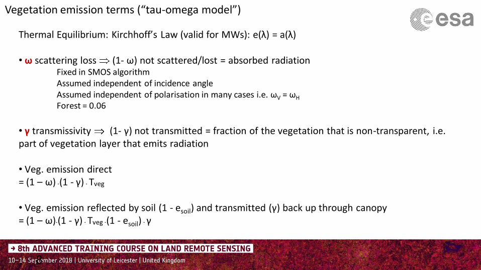
Thermal Equilibrium: Kirchhoff’s Law (valid for MWs): e(λ) = a(λ)

• ω scattering loss (1- ω) not scattered/lost = absorbed radiationFixed in SMOS algorithmAssumed independent of incidence angleAssumed independent of polarisation in many cases i.e. ωV = ωH

Forest = 0.06

• γ transmissivity (1- γ) not transmitted = fraction of the vegetation that is non-transparent, i.e. part of vegetation layer that emits radiation

• Veg. emission direct = (1 – ω) ∙(1 - γ) ∙ Tveg

• Veg. emission reflected by soil (1 - esoil) and transmitted (γ) back up through canopy= (1 – ω)∙(1 - γ) ∙ Tveg ∙(1 - esoil) ∙ γ

8

Vegetation emission terms (“tau-omega model”)

TB,tot(P,θ) = esTsγ + (1 – ω) (1 - γ)Tv + (1 – ω) (1 - γ)Tv (1 - es)γ + TB,skyγ2 (1 - es)

es soil emissivity; linked to soil moisture through dielectric constantTs physical temperature of soilTv physical temperature of vegetationω single scattering albedo of vegetation (omega)γ canopy transmissivity; linked to vegetation optical depth τ (tau)TBsky sky brightness temperature

P polarisation (H or V)θ incidence angle

1. soil 2. vegetation 3. vegetation-soil 4. sky

9

10

Vegetation Optical Depth (τ)

e cos

• τ : at Nadir • Depends on :

- biomass density- structure- vegetation water content

X band= 3 cm

L band= 21 cm

P band= 70 cm

VHF>3 m

©Biomass Cesbio

• Vegetation « seen » at various wavelengths

• ESA (European Space Agency) - Level 1:

L1a: Visibilities L1b: Fourier Coefficients L1c: Brightness Temperatures , polarization X/Y (antenna frame)

- Level 2 : Surface Soil Moisture, salinity

• Centre Aval de Traitement des Données SMOS CATDS - Level 3: Brightness temperatures, polarization H/V- Level 3: Soil moisture & VOD, dielectric constant- Level 4: SMOS + model hydro (Root Zone Soil Moisture ; Drought Index ; desaggregation ...)

• BEC Spain : Barcelona Expert Center- Level 3 et 4 Aggregation of ESA products

SMOS Data

Swath Product Aggregated Product

Known as ESA Level 2 CATDS Level 3

Algorithm Use of 1 overpass Use of 3 consecutive overpassesCorrelation of the vegetation optical depth

Derived soilmoisture

One per ½ orbit 1 day3-day10-daymonthly products

Format BinX ; Netcdf Netcdf

Grid Isea4h9 ~15 km EASE Grid ~25x25km

Level 3 : Al Bitar et al. 2017, ESSD

● per ½ orbitAscendingDescending

UDP : User Data Product

● 2 files: .HDR Header .DBL Datablock, BINARY file containing the data

● L2 soil moisture GridISEA4h9spatial resolution ~15 km

~15km ●●

● ●

●●●

●

●

SMOS Level 2 land products

UDP -User Data Product-Parameters of the model

SM TAU DQX = index, quality of the retrieval NOT an error compared to in-situDielectric constant TB @ 42.5° from models!RFI_ProbCHI2

• Science flagsInformation about the conditions: forest, topography, rain, snow...

• Confidence flagsEvaluation of the retrieval:

retrieval failed (FL_NO_PROD)is retrieved soil moisture within an expected range? its DQX ? quality of the modelsRFI contaminations

• Processing FlagsConditions of the retrieval: model used, initial conditions.…

Successful retrieval = valueFailed retrieval = -999

SMOS Level 2 land products

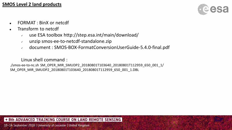
FORMAT : BinX or netcdf Transform to netcdf

use ESA toolbox http://step.esa.int/main/download/ unzip smos-ee-to-netcdf-standalone.zip document : SMOS-BOX-FormatConversionUserGuide-5.4.0-final.pdf

Linux shell command : ./smos-ee-to-nc.sh SM_OPER_MIR_SMUDP2_20180801T103640_20180801T112959_650_001_1/SM_OPER_MIR_SMUDP2_20180801T103640_20180801T112959_650_001_1.DBL

SMOS Level 2 land products

Objectives

Present VOD (Vegetation Optical Depth) derived from SMOS

Access the data using Matlab

>> p='SM_OPER_MIR_SMUDP2_20180801T121643_20180801T131004_650_001_1.nc'

p =

SM_OPER_MIR_SMUDP2_20180801T121643_20180801T131004_650_001_1.nc

>> info=ncinfo(p)

info =

Filename: [1x120 char]Name: '/'

Dimensions: [1x1 struct]Variables: [1x72 struct]Attributes: [1x370 struct]

Groups: []Format: 'netcdf4'

>> info.Variables.Name>> info.Variables. Attributes

General information

• File content• Attributes of field

Field ValuesOffsetScale Factor …

>> vod=ncread(p,'Optical_Thickness_Nad');

>> load coast ; >> figure >> scatter(lon_smos,lat_smos,15,vod,'filled')>> hold on ;>> plot(long,lat,'-k') ;

• Get the VOD from the product

• Display the VOD

• Get Latitudes and Longitudes of all nodes

>> lat_smos=ncread(p,'Latitude') ;>> lon_smos=ncread(p,'Longitude') ;

Rq : data are vectorsNb of points varies from a product to another

>> days = ncread(p,'Days') ;>> sec = ncread(p,'Seconds') ;>> microsec = ncread(p,'Microseconds') ;

>> dayref_smos = datenum(2000,01,01) ;>> time_smos = dayref_smos + days + sec* 1/86400 + (microsec)*1e-6* 1/86400 ;>> time_smos(isnan(time_smos)) = [] ; % Remove nan values >> datestr(time_smos)

• Extract the time

>> dgg=ncread(p,'Grid_Point_ID') ;

>> figure >> scatter(lon_smos,lat_smos,15,dgg,'filled') ; >> hold on ; >> plot(long,lat,'-k')

Rq : For time series- find the DGG of interest, get its position in the product

• DGG ID

One Node = one id

• DGG ID

>> p='SM_OPER_MIR_SMUDP2_20180801T121643_20180801T131004_650_001_1.nc‘ ;>> vod=ncread(p,'Optical_Thickness_Nad') ;>> size(vod)ans =

66635 1>> p='SM_OPER_MIR_SMUDP2_20180801T103640_20180801T112959_650_001_1.nc‘ ;>> vod=ncread(p,'Optical_Thickness_Nad') ;>> size(vod)ans =

116384

• RFI (Radio frequencies Interferences)

- Sources emitting at L-band…but should not- Affect SMOS TB and so the derived SM-VOD

>> rfi = ncread(p,'RFI_Prob') ;

Strategy to start with the SMOS data

• SM -999 and within the range [0 - 0.7] m3/m3

• SM_DQX -999 & SM_DQX < 0.1 m3/m3< 0.07 (L2SM SMOS Report) < 0.099 (Bircher et al.)< 0.06 (dall Alamico et al. 2012)

• N_RFIX + N_RFIY / M_AVA0 : RFI of the day ! <0.05/0.1 ; <0.04 (Bircher et al. 2013) tested at the Danish site with a lot of RFI

• P_RFI < 10 %RFI over a long period: if one source switched on, then affects the P_RFI for a long time period

• Temperature> 0°

Deeper analysis• Flags: Understand the retrieval conditions (rain …)• Fraction : FM0 (for instance forest => FM0_FO> 90%)

NOTE: Thresholds can be adjusted to your site

Other Tools

• NCO : nco.sourceforge.net• Python• GDAL • Panoply (Nasa, Netcdf grib viewer) • ESA toolbox

SNAP + SMOS toolbox

https://earth.esa.int/web/guest/missions/esa-operational-eo-missions/smos/content/-/asset_publisher/t5Py/content/data-reader-software-7633

References

*) Rahmoune et al. 2013IEEE Journal of Selected Topics in Applied Earth Observations and Remote Sensing, Vol 6, n. 3, June 2013

*) Vittucci et al. 2016, Remote Sensing of Environment, 180, 115–127

*) Vittucci et al. 2017, IEEE Geoscience and Remote Sensing Letters, vol. 14, n. 12

*) Parrens et al. 2017, IEEE Geoscience And Remote Sensing Letters

*) Rodríguez-Fernández et al. 2018 Biogeosciences, 15, 4627–4645, 2018