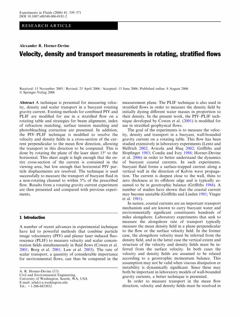
RESEARCH ARTICLE

Alexander R. Horner-Devine

Velocity, density and transport measurements in rotating, stratified flows

Received: 15 November 2005 / Revised: 25 April 2006 / Accepted: 13 June 2006 / Published online: 8 August 2006� Springer-Verlag 2006

Abstract A technique is presented for measuring veloc-ity, density and scalar transport in a buoyant rotatinggravity current. Existing methods for combined PIV andPLIF are modified for use in a stratified flow on arotating table and strategies for beam alignment, indexof refraction matching, surface tension matching andphotobleaching correction are presented. In addition,the PIV–PLIF technique is modified to resolve thevelocity and density fields in a cross-section of the cur-rent perpendicular to the mean flow direction, allowingthe transport in this direction to be computed. This isdone by rotating the plane of the laser sheet 15� to thehorizontal. This sheet angle is high enough that the en-tire cross-section of the current is contained in theviewing area, but low enough that horizontal PIV par-ticle displacements are resolved. The technique is usedsuccessfully to measure the transport of buoyant fluid ina non-rotating channel to within 5% of the prescribedflow. Results from a rotating gravity current experimentare then presented and compared with previous experi-ments.

1 Introduction

A number of recent advances in experimental techniquehave led to powerful methods that combine particleimage velocimetry (PIV) and planar laser induced fluo-rescence (PLIF) to measure velocity and scalar concen-tration fields simultaneously in fluid flows (Cowen et al.2001; Borg et al. 2001; Law et al. 2003). The rate ofscalar transport, a quantity of considerable importancefor environmental flows, can thus be computed in the

measurement plane. The PLIF technique is also used instratified flows in order to measure the density field byinitially dyeing different water masses in proportion totheir density. In the present work, the PIV–PLIF tech-nique developed by Cowen et al. (2001) is modified foruse in stratified geophysical flows.

The goal of the experiments is to measure the veloc-ity, density and transport in a buoyant, wall-boundedgravity current on a rotating table. This flow has beenstudied extensively in laboratory experiments (Lentz andHelfrich 2002; Avicola and Huq 2002; Griffiths andHopfinger 1983; Condie and Ivey 1988; Horner-Devineet al. 2006) in order to better understand the dynamicsof buoyant coastal currents. In such experiments,buoyant fluid forms a surface-trapped current along avertical wall in the direction of Kelvin wave propaga-tion. The current is deepest close to the wall, thins tozero thickness at its offshore edge and is typically as-sumed to be in geostrophic balance (Griffiths 1986). Anumber of studies have shown that the coastal currentmay become unstable (Griffiths and Linden 1981; Vingeret al. 1981).

In nature, coastal currents are an important transportmechanism and are known to carry buoyant water andenvironmentally significant constituents hundreds ofmiles alongshore. Laboratory experiments that seek tomeasure the alongshore rate of transport typicallymeasure the mean density field in a plane perpendicularto the flow or the surface velocity field. In the formercase, the alongshore velocity must be inferred from thedensity field, and in the latter case the vertical extent andstructure of the velocity and density fields must be in-ferred from the surface velocity. In both cases thevelocity and density fields are assumed to be relatedaccording to a geostrophic momentum balance. Thisassumption may not be valid when viscous dissipation orinstability is dynamically significant. Since these mayboth be important in laboratory models of wall-boundedgravity currents, a better technique is presented.

In order to measure transport in the mean flowdirection, velocity and density fields must be resolved in

A. R. Horner-Devine (&)Civil and Environmental Engineering,University of Washington, Seattle, WA, USAE-mail: arhd@u.washington.eduTel.: +1-206-6853032

Experiments in Fluids (2006) 41: 559–571DOI 10.1007/s00348-006-0181-2

a vertical plane perpendicular to the mean flow. This isdone by rotating the plane of the co-aligned PIV andPLIF laser sheets relative to the horizontal. When thecorrect angle is chosen, PLIF dye concentrations andalong-wall PIV displacements can be resolved simulta-neously across the vertical and cross-shore extent of thecurrent, allowing calculation of the alongshore rate oftransport. Since the vertical structure of the current isbased on a projection from the angled plane of the sheet,the technique is limited to flows for which the scale ofalongshore variability is greater than the alongshoreextent of the measurement area.

The technique is validated in a series of non-rotatingexperiments with a known transport rate. Techniquesare presented that correct for the effects of index ofrefraction, photobleaching and variation of surfacetension. In further experiments on a rotating table thestructure of the current is investigated and is comparedwith previous rotating gravity current experiments.

2 Experimental setup

All of the experiments were conducted in an annulartank on a 2-m rotating table (Fig. 1). The table, whichconsists of a circular steel plate attached to a rectangularbase by means of a large thrust bearing is level to within10�5. A servo motor (Pacific Scientific, model R8AG,50 Nm maximum torque) with a 50:1 orbital gear head(Bayside Motion Group) drives the table with a non-slipdrive belt. The motor speed and acceleration are con-trolled by a PC computer with Galil Motion Controlsoftware, in conjunction with a motor controller(Compumotor). This system provides accurate controlof the rotation speed and allows very smooth rotation.

The water tank is a 500 l Plexiglas annulus that is25 cm deep and has 184 and 44 cm diameter outer andinner walls, respectively. The tank is outfitted with a0.5 cm thick Plexiglas lid to prevent surface stress due towind shear. A 155 cm high three-legged frame, whichstraddles the entire tank, supports a high fidelity slip ringand a digital camera mount. The slip ring is used tobring electrical power and a TTL trigger signal onto thetable. A second smaller frame is used for on-table elec-tronic components including a image acquisition com-puter and digital camera controller.

The current is generated along a straight 120 cmPlexiglas interior wall set across one side of the tank.The end section of the wall is hinged so that it makes aright angle with the wall. Buoyant water is introducedinto the tank at the level of the water surface through a5 cm · 1 cm slot by means of a diffuser affixed to theback of the hinged section. The diffuser is a 6.25 cm3

chamber filled with small plastic beads. Typical flowrates range from 3 to 16 cm3 s�1 resulting in diffuserresidence times less than 1.0 s. The adjustment time forthe flow is approximately one rotation period (10–40 s),so the inflow rate can be considered to ramp upinstantaneously.

Two experimental configurations are used to generatea buoyant current in a non-rotating and rotating system,respectively. In order to measure the total volume flux,the current must be limited to a width that is less thanthe field of view in both cases. This is satisfied in therotating case as the current is held against the wall dueto Coriolis acceleration. In order to test the technique inthe experimentally simpler non-rotating case, it wasnecessary to contain the current within a channel. Thechannel is 5 cm wide and consists of two Plexiglas wallsthat are installed along the coastal wall in the tank such

Directionof rotation

Coastal wall

Diffuser(W=5cm,H=1cm)

Freshwatersource

Tank wall (r = 92cm)

Inner tankwall (r = 22cm)

Overflowstandpipe(R=8cm,H=20.5cm)

Fieldof view

Angled laser sheet

A B

Coastal current

Main steel base

Opticsbreadboard

Rotatingsteel base

Electrical slip ring

Outer tankwall

Inner tank wall

Tank

YAG and Ar+

laser beampath

Turningmirror

Cylindricallens

Angled laser sheet

Water level22cm

Three-leggedframe

Table bearing

Digitalcamera

Coastalcurrent

a) b)

Fig. 1 Schematic of the rotating table viewed from the side a, andof the tank configuration viewed from above b. The orientation ofthe angled laser sheet is included in both schematics. In b the side of

the sheet labeled B extends above the water surface and A extendsbelow the buoyant current

560

that the non-rotating current occupies approximatelythe same space as the rotating current. Buoyant wateris introduced to both the rotating and non-rotatingcurrents using the source described below. In the non-rotating configuration, the buoyant fluid forms a two-layer flow that is discharged from the channel into thelarger tank on the downstream end. The experimentbegins after the channel flow has reached steady state.

We measure the flow rate with a ball float flow meterimmediately before the flow passes through a slip ringonto the table. The source water is discharged from aconstant head system 2.4 m above the rotating table thatconsists of two 60 l Nalgene tanks. The temperature ofthe buoyant source and ambient tank water is measuredusing a 0.01�C resolution thermistor (Fluke Y2039). Thetemperature in the room is also measured with a± 0.5�C wall thermometer, since the thermistor picksup noise from the table servo motor when it is enabledand therefore cannot be used during a run. The densityis measured with a ± 5 · 10�5 g cm�3 oscillatingU-tube density meter (Anton-Paar, model 4500).

PIV and PLIF images are illuminated using a pair ofpulsed ND:YAG lasers (120 mJ Gemini PIV, New WaveLaser) and a continuous wave Argon ion laser (5 WInnova 305, Coherent) and imaged with a 30 Hz,1 k · 1 k, 12 bit CCD camera (SMD1M30_10 SiliconMountain Designs, now Dalsa Corporation). The lasersare mounted on a large optics breadboard beneath therotating table (Fig. 2). Beam steering optics and a thinfilm polarizer on the breadboard are used to focus andco-align all three beams. The co-aligned beams are thendirected upward through a 6 mm diameter hole in thecenter of the table. An angled mirror fixed to therotating table steers the beams horizontally through apair of cylindrical lenses to create a light sheet in therotating frame of reference.

3 Measurement technique

In order to calculate the alongshore transport of buoy-ant fluid in the current, PIV and PLIF are used tomeasure the velocity and density fields, respectively, inan angled cross-sectional slice of the current.

3.1 Combined velocity and density measurement

Combining PIV and PLIF presents a challenge, sinceimplementation of the former requires that the flow isseeded with particles that reflect light and introduce er-rors in the measured concentration field. Conversely,emitted light from the PLIF dye can contaminate thePIV images. A number of solutions have been presentedto circumvent this problem (Cowen et al. 2001; Borget al. 2001; Law et al. 2003). The present experimentsemploy the single camera solution of Cowen et al.(2001). Each snapshot consists of three images, two PIVand one PLIF, which are acquired within 0.1 s. A sharp514 nm cut-off filter is mounted to the camera to dis-tinguish between the two desired image types. The PIVimages are illuminated with the 532 nm ND:YAG la-sers. The wavelength of the reflected light from theparticles is also 532 nm so it passes through the filter.The PLIF image is illuminated with the Argon ion laser,which has a wavelength of 488 nm. To be successful, thePIV/PLIF technique requires that emitted light from thefluorescent dye passes through the filter, however, lightfrom Argon ion laser reflecting off the particles does not.This is achieved by choosing the appropriate fluorescentdye. Fluorescein is used since its excitation and emissionbands are centered at 490 and 530 nm, respectively.There are two known drawbacks to using Fluoresceinfor PLIF; it can be very sensitive to pH (Walker 1987)and is prone to photobeaching (Crimaldi 1997). Tech-niques for minimizing errors due to these two effects arepresented below.

3.2 Velocity measurement

Implementation of PIV Particle image velocimetry hasbeen used extensively in fluid mechanics experiments tomeasure fluid velocity. The reader is referred to Raffelet al. (1998) for a thorough introduction to the techniqueand to Sveen and Cowen (2004) or Liao and Cowen(2005) for a discussion of some recent improvements.Digital PIV involves imaging a cross-section of a particle-seeded flow and then numerically interrogating sequentialpairs of images to determine mean particle displace-ments. The technique uses spatial cross-correlation ofsub-windows within the image to determine the dis-placements from which the velocity is calculated. In thisstudy, second order accurate codes written by Cowen areused to compute particle displacements (Cowen et al.2001; Cowen and Monismith 1997). The images are

YAGlaser A

rgon

ion

lase

r

M1 M2 M3 M4

M5

M6

L1: f = 76mm L2: f = -38mm W1: λ/2

W2: λ/4

TFP

Shutter

Fig. 2 Schematic of the laser optics (plan view). Components arelabeled as follows. M mirror, L lens, W waveplate and TFP thinfilm polarizer. Mirror 6 is oriented at 45� to the horizontal so thatthe beam is directed vertically through the center of the table. Thedashed, dotted and solid lines are the Argon ion, YAG andcombined beams

561

initially interrogated in 64 · 64 pixel sub-windows. Thesub-window size is then decreased iteratively to 32 · 32and then 16 · 16 pixels using the results of the coarserpass to offset the sub-windows at the finer resolution. Inaddition to decreasing the sub-window size, the width ofthe weighting function used to account for the correlationbias error was successively decreased on each pass.

Particle seeding In order to accurately measure thevelocity in the flow using PIV, it is necessary to haveparticles dispersed uniformly in the flow. Since thepresent flow is stratified and since the ambient flow isquiescent, very small particles (Potters Industries,Spherical Hollow Sphere, qp = 1.1 g cm�3, dp . 11 lm)were used, which have a fall velocity of 7 · 10�4 cm s�1

based on Stokes law. Based on this estimate of the fallvelocity, particles are expected to fall approximately3.6 cm during the 90 min. tank spin-up period. It wassometimes necessary to add particles to the tank duringthe spin-up in order to ensure that there was adequatecoverage, however, we generally did not have troublekeeping enough particles in the images. The particleseeding density was greater than 10�6 by mass, whichresulted in approximately 20 particles per 32 · 32 pixelsub-window. This exceeds the minimum desirable countdetermined by Cowen and Monismith (1997).

Temporal and spatial resolution The timing signal isgenerated for PIV and PLIF images using a digital delaygenerator (Berkeley Nucleonics), which has a resolutionof 1 ns. The spacing between PIV images is 40 msand images triples are acquired at 1 Hz. For calibration,an image of a 10 · 10 cm clear grid is acquired in theplane of the laser sheet. We manually interrogate outerpoints in the grid image to calculate the dimensionalmagnification of the optical system, which is M =0.013 cm pixel�1. Further sub-sampling of the imageconfirmed that the magnification was spatially uniformto within one pixel. Higher accuracy could be achievedby interrogating the grid digitally and solving the over-determined system to compute the mapping for eachpoint independently, as described in Raffel et al. (1998).The current calibration technique is considered to beadequate for resolving the mean flow properties in thecurrent. However, there is no reason that higher accu-racy techniques could not be implemented if they werejustified. The displacement fields are converted tovelocity fields according to

u; vð Þ ¼ DxMDt

;DyMDt

� �:

Finally, we filter the velocity fields using a 3 · 3median filter to get rid of outliers. The physical width ofeach image is 13 cm, resulting in a nominal spatial res-olution of 0.2 cm. This corresponds to the resolution inthe direction perpendicular to the wall. The verticaldimension is obtained by projecting the angled along-wall dimension of the image into a vertical plane. Theeffective vertical resolution is 0.05 cm.

Index of refraction Optical measurement techniquessuch as PIV and PLIF are challenging in a stratified fluidbecause variation in fluid density is usually also associ-ated with variation in index of refraction, n. The varia-tions in n distort the incident laser sheet path resulting insome ambiguity in the sheet location. The path of thelight reflected from particles and emitted from the dye isalso distorted, resulting in blurring of the image as wellas position ambiguity. Both of these significantly de-crease the accuracy of PIV and PLIF. Alahyari andLongmire (1994) find that aqueous solutions of glyceroland potassium phosphate could be used to obtain fluiddensity differences while matching the index of refrac-tion. They show that PIV accuracy improved signifi-cantly with matched indices of refraction. We useisopropyl alcohol (rubbing alcohol or 2-propanol) andsalt to match n since they are readily available and eco-nomical. It has been used successfully for PIV and PLIFexperiments by Lowe et al. (2002) and Troy and Koseff(2005). In the range of densities that are relevant to thisstudy, the variation of n with density is approximatelylinear and given by,

na ¼ 1:9802� 0:6499qa; ð1Þns ¼ 1:0924� 0:2411qs; ð2Þ

for alcohol and salt solutions (Fig. 3). Each densitydifference, therefore, corresponds to a single index ofrefraction.

For a desired Dq = qs � qa, qs and qa are chosen sothat n is matched. Rearranging Equations 1 and 2, thematched index of refraction nm is expressed in terms ofDqqs

as

nm ¼4:5313 Dq

qs� 7:5782

4:1479 Dqqs� 5:6867

ð3Þ

A potential drawback of using isopropyl alcohol forindex of refraction matching is that alcohol has a higherviscosity than water. For the majority of runs we use1.8% alcohol, corresponding to an increase in the vis-cosity of the solution of less than 10%.

Surface tension Adding alcohol to the source wateralso reduces the surface tension of the fluid. The surfacetension of pure isopropyl alcohol is 20.93 dyn cm�1

compared with 71.99 dyn cm�1 for pure water. Thisdifference drives a surface flow when the alcohol–watersolution from the source comes in contact with theambient salt water. The source water moves radiallyaway from the source across the surface of the waterimmediately after the source is turned on. The spreadingis eventually arrested due to friction, leaving a thinbuoyant layer that extends offshore well beyond the edgeof the buoyant current. This layer is eventually acceler-ated by Coriolis and forms a distinct current. Since thecurrent induced by the surface tension difference drawsboth mass and momentum from the primary current, itcauses noticeable deviations in the dynamical descrip-tion of the flow.

562

In order to avoid this source of error, a small amount(25 ml) of strong commercial surfactant (Kodak Photo-Flo 200) is added to the tank prior to the run. Wedetermined the appropriate concentration of surfactantby incrementally increasing the concentration in asample container of ambient tank water until a drop ofsource fluid released on the surface no longer induced apronounced surface flow. We adjust the concentration ofsurfactant for runs with different g¢ and thus differentalcohol concentration.

3.3 Density measurement

Implementation of PLIF Planar laser induced fluores-cence is used to measure the density field in the flow. Thetechnique involves illuminating the desired field of viewwith a thin laser sheet and adding a known concentra-tion of fluorescing dye to the buoyant source water. Thedye and laser combination is chosen so that the dye (inour case fluorescein) is optimally excited at the wave-length of the illuminating laser light (in our case 488 nmfrom the Argon ion laser). When it is excited, the dyeemits light at a higher wavelength and its intensity isproportional to both the incident laser light intensityand the local dye concentration. The distribution andintensity of emitted light in the laser sheet is measuredwith the CCD chip in the digital camera. After properlycorrecting for the distribution of incident laser intensity,the intensity in the acquired PLIF images is correlatedwith the dye concentration. Thus, high intensity regionsin the image correspond to regions in the flow with highdye concentration. Since dye is added to the buoyantinflowing fluid in a known amount, the fluid density cansubsequently be computed from the dye concentrationfield. Below we describe the implementation, correc-tions, and calibration of PLIF that were used for thepresent experiments.

In order to calculate the dye concentration, Cn(i,j),from the acquired digital images, we follow the methoddescribed in Crimaldi and Koseff (2001). Here the pixelindices are 1 < i < 1,024 and 1 < j < 1,024, and n isthe image index. In this method, variations in dye fluo-rescence, laser sheet intensity, and pixel response in theacquired digital image An(i,j) are accounted for using abackground image Bn(i,j) with a low, spatially uniformdye concentration and a dark response image D(i,j). Theeffectiveness of the background image correction tech-nique relies on the assumption that the chemical prop-erties of the water, the laser sheet illumination, and thepixel response are identical in An(i,j) and Bn(i,j).Assuming that this is true, the corrected image A¢n (i,j) iscomputed according to

A0nði; jÞ ¼Anði; jÞ � Bnði; jÞBnði; jÞ � Dði; jÞ : ð4Þ

For each experiment, the dark response image D(i,j)is obtained by averaging 50 images immediately after theexperiment in a completely darkened room with the lenscap on. Acquiring the background image is more in-volved since very small variations in the optical align-ment result in illumination that varies as the table isrotated. This requires that a separate background imageis acquired for each PLIF image in the experiment.These background images are acquired before eachexperiment using the same timing and illumination, butwith only a low, uniform concentration of Fluorescein inthe tank.

For the present experiments, the background dyeconcentration is not easily measured, therefore, theconcentration is calibrated relative to the undiluteddye concentration of the source water. The ambientdye concentration is very small relative to the sourceconcentration and is assumed to be zero for the purposesof calibration. A separate image of undiluted sourcewater, Asrc, is acquired prior to the run for the calibra-tion. A corresponding background image is alsoacquired and Asrc is processed using Eq. 4. The averageintensity is found in the region of the corrected imageA¢src that corresponds to the undiluted source waterso that we have a scalar representing the maximumconcentration. In practice, three methods are used tomeasure the scalar intensity of the undiluted sourcefluid, asrc, based on spatial averaging of the correctedimage A¢src. In the first method, source fluid is dis-charged through a 2 mm diameter nozzle forming a jetin the plane of the laser sheet. Ten images of the jet areaveraged and corrected as above. The scalar intensitycorresponding to the source water, asrc, is the averageintensity in the 10 · 10 pixel region corresponding to thepotential core of the jet. In the second method, a26 · 11 · 9 cm Plexiglas box is filled with source fluidand placed in the laser sheet so that it is illuminatedthrough the long side. A composite average image isgenerated from ten images and corrected for attenuation(see Sect. 3.3.1). The composite image is further averaged

1.33 1.332 1.334 1.336 1.338 1.34 1.342 1.344 1.346 1.348 1.350.97

0.98

0.99

1

1.01

1.02

1.03

1.04

1.05

1.06

1.07

1.08

n

ρ, g

cm

–1alcoholsalt

Fig. 3 Variation of density with index of refraction for isopropylalcohol (2-propanol) and salt (sodium chloride). The lines representlinear regressions to the first 12 points. Data are from Lide (2003)

563

across the image to obtain a single intensity profile. Thescalar intensity corresponding to the source water, asrc,is the maximum intensity in the averaged profile (Fig. 4).In the third method, the maximum pixel intensity in auniform flow in the rectangular test channel is used. Thisvalue is obtained by averaging the intensity in the regionof unmixed fluid in the buoyant surface layer. Althoughall three methods resulted in comparable values for thesource intensity, the third generated the most consistentcalibration.

If we assume that the background concentration, thebackground image, and the dark response are the samein the source images as in the images taken during therun, we can normalize the run images by the maximumconcentration in the source image, a¢src, and obtain thescaled dye concentration

Cði; jÞCo

¼ Aði; jÞ0a0src

:

Finally, the density anomaly is obtained from thescaled concentration field according to

qði; jÞ ¼ qa �Cði; jÞ

Coqs;

where qa and qs are the ambient and source fluid densities,respectively. When calculating the transport of buoyantfluid, the scaled concentration Cði;jÞ

Cois used directly to

represent the scaled buoyancy anomaly (qa � q)/qs.

3.3.1 Attenuation

The intensity of laser light is attenuated in proportion tothe concentration of dye and PIV particles present.Attenuation due to water alone and background con-centrations of dye and particles is accounted for with thebackground correction described above. When buoyant

water is present, however, the attenuation depends onthe instantaneous distribution of dye and particles in theimage. Dye concentration in the image is under-pre-dicted as a result of the decrease in the local laser sheetintensity caused by attenuation. Cowen et al. (2001)describe this problem and establish a solution techniquethat is the basis of the correction used in the presentwork. The interested reader is referred to their paper fora complete description of the theory and validation ofthe technique.

In order to correct for the variation in laser intensity,the attenuation must be estimated at each point in thesheet. Following Cowen et al. (2001), an effectiveattenuation coefficient geff is determined that accountsfor dye and particles together. The coefficient is esti-mated based on the source box intensity profile (Fig. 4)according to

geff ¼ �1

x2 � x1log

I2I1

� �;

where (x1,I1) and (x2,I2) are points in the linearlydecreasing section of the profile between 400 and 900pixels. The true concentration at each point depends onthe concentration along the path after it has been cor-rected for attenuation and so the correction must beapplied recursively. The attenuation is calculated pro-gressively along the beam path and the concentration iscorrected for attenuation at each step before the atten-uation is calculated for the next point along the beampath. Finally, the concentration is corrected based onthe new value for the laser intensity at each point.

In the above technique, the attenuation coefficient ismeasured using sample fluid that includes dye and par-ticles so that, while only dye concentration is measuredin the images, both are included in calculating the laserattenuation. An assumption has been made, therefore,that the mixing rates of the dye and particles are similar.This assumption has not been tested explicitly in thepresent work. However, the success of the technique formeasuring transport indicates that it is reasonable.

3.3.2 pH compensation

The efficiency with which dissolved fluorescein emits lightis known to be a strong function of the pH of the solution(Walker 1987). The variation in emission with pH isgreatest in the range between pH = 6 and 8, withlow emission for solutions with pH < 6. For pH > 8,emission is maximized and is effectively independent ofpH. In order to avoid the effects of pH, therefore, webuffer both the tank and source water using sodium car-bonate (Na2CO3) to greater than pH = 8.5 for each run.

3.3.3 Surface location

Image-based experiments in near-surface flows presentan additional challenge since the exact location of the

100 200 300 400 500 600 700 800 900 10000

0.2

0.4

0.6

0.8

1

1.2

pixels

I/I o

UncorrectedCorrected

Fig. 4 Normalized intensity in a box of source fluid with andwithout correction for attenuation. Io is the maximum intensity inthe raw profile. The walls of the box are 350 and 930 pixels from theleft side of the image

564

surface must be determined in the image. This is com-plicated in the present experiments since the angled lasersheet reflects off the surface and illuminates regions ofthe image that are not in the desired flow cross-section.Accurate location of the surface is necessary for com-puting the transport in the image cross-section. Twotechniques were compared for determining the surfacelocation. In the first, a series of PIV images were aver-aged. Since a few buoyant particles inevitably collect onthe water surface, a clear band of higher intensity pixelscorresponding to these particles is evident in the images.The surface location is taken to be the location ofmaximum intensity in the average, smoothed intensityprofile. The second technique identifies the surface in asimilar fashion in the PLIF image. Both techniquesprovided similar results. The standard deviation of thesurface location was 16 pixels over the course of oneexperiment based on the PLIF technique. Since the sheetis inclined, this corresponds to 0.05 cm in the verticaland an error in the transport measurements of less than5%. For the purposes of the transport calculations, anaverage value of the surface location was used.

3.4 Angled sheet

In order to capture the entire cross-section of thecurrent, the YAG and Ar+ laser sheets are angledrelative to horizontal. To generate each sheet, laserlight is directed outward from the center of the tablethrough a cylindrical lens. The axis of the sheet ishorizontal and perpendicular to the coastal wall andflow direction (Fig. 1). The sheet is rotated about itsaxis such that the upstream edge is below the currentand the downstream edge is above it. The camera isrotated by approximately the same amount as thesheet. The camera angle is fine-tuned with the illumi-nated grid plate in place to ensure that the entire fieldof view is in focus.

Since the sheet has a finite thickness (� 1.5 mm),particles that are displaced horizontally by a smallamount stay in the sheet and have a measurable dis-placement in the angled plane of the sheet (Fig. 5). Er-rors in the measured along-shore velocity are minimizedwhen the sheet angle hs is small.

The actual horizontal displacement, Dx, is mappedinto the viewing plane, Ds, according to Ds = Dx cos hs.The in-sheet displacements are converted to actual dis-placements by inverting this relationship,

Dx ¼ Dscos hs

:

It is important to note that the technique cannotdifferentiate between vertical and horizontal velocities.However, a low sheet angle reduces the contribution tothe measured displacement, Ds¢, by a vertical displace-ment, Dz according to

Ds0 ¼ Dz sin hs:

The error in Ds due to a vertical displacement is givenby

Ds0Ds¼ Dz

Dxtan hs:

According to the continuity equation Dz=Dx � h=L:For the rotating gravity current, a conservative estimateof the representative length scale, L, in the coastal cur-rent is the Rossby radius, Lr ¼ ðg0hÞ=f ; whereg0 ¼ gDq=q; f is the Coriolis frequency and h is the localcurrent depth. For typical flow parameters, h = 1 cmand Lr = 5.3 cm. This gives an estimate for the errordue to velocity ambiguity of 5%.

A vertical cross-section of the current is obtained byprojecting the resolved velocity field from the angledsheet onto a vertical plane, where the vertical coordinateis given by z = s sinhs. The projected cross-sectionaccurately describes a vertical section of the currentif the scale of along-wall variability in the current ismuch greater than the length of the measurement area,s coshs = 12.6 cm. Near the gravity current head thescale of variability is expected to be on the order of theRossby radius. Thus the projected section will not berepresentative of a vertical section. Far from the head ofthe current, however, the scale is expected to be muchlonger and the projected vertical section will be accurate.

3.4.1 Photobleaching

Fluorescein dye is known to be susceptible to photo-bleaching, whereby the emission efficiency of dye mole-cules depends on the duration of exposure to laser lightCrimaldi (1997). Photobleaching introduces errors intothe concentration measurements since emission from thedye depends on its residence time in the laser sheet andthus the velocity. Crimaldi (1997) showed that the flu-orescence, F, at a single point normalized by theunbleached fluorescence, Fo, is

FFo¼ 2

p

� �3=2

expð�BpbÞ;

where Bpb is a photobleaching parameter given by

θ=15o

Laser Sheet

∆x

∆s

ρbuoyant

ρambient

View

ing

angle

Fig. 5 Displacement schematic for the angled slice technique. Viewfrom the coastal wall side

565

Bpb ¼PQbr

ð2pÞ1=2ahmU:

In the above expression, P is the laser power, Qb isthe quantum bleaching efficiency, r is the absorptioncross-section, 2a is the e�2 beam width, h is Planck’sconstant, m is the frequency of the laser light and U is thefluid velocity. Higher values of Bpb result in morephotobleaching and greater error on the fluorescence.

Crimaldi (1997) provides a numerically integratedsolution for the fluorescence in a measuring volume,which is appropriate for a laser sheet with finite width.Since Bpb is an inverse function of velocity, the fluores-cence, and therefore the concentration, will be underpredicted in regions of the current where velocity is low.It is important to note that errors in concentrationmeasurement in slow regions of the current contributerelatively small errors to the totally flux measurement.Nonetheless, because we know the velocity at each pointin the density field, we can estimate and correct for theerrors due to photobleaching. In order to make thecorrection computationally tractable, we estimate thenumerically integrated function used by Crimaldi as

FFo¼ expð�Bpb=2Þ: ð5Þ

The fluorescence decreases rapidly for0.01 < Bpb < 10 (Fig. 6).

In our case, P = 1 W (where we have accounted forlosses in the optics system), Qb r = 2.8 · 10�24 m2 (asreported by Crimaldi (1997) for fluorescein),a = 7.5 · 10�4 m, h = 6.621 · 10�34 Js, m = 6.1475 ·1014 s�1 and U @ 1 cm s�1. This gives a value ofBpb = 0.37, for which F =Fo ¼ 0:83: Since much of theplume will have U < 1 cm s�1, the local error in theuncorrected concentration field due to photobleachingwill be at least 17% is these slow regions.

In order to correct the entire concentration field, thecomputed velocity field U(i,j) is used to calculate anarray of Bpb(i,j) values corresponding to each point inA(i,j). The reduction in fluorescence, F =Fo at each pointis then calculated according to Eq. 5. Finally, the cor-rected concentrations are calculated according to

Acorrected ¼A

F =Fo

The correction algorithm has difficulty in regions outsidethe plume where U(i,j) fi 0, and therefore Bpb fi ¥and F =Fo ! 0: If there is a trace amount of dye abovethe background level, then the corrected concentrationwill be very high. In order to avoid this, we set F =Fo ¼ 1for regions of the image where U < 0.05 cm s�1. Sincethe cut-off velocity is very small, however, this correc-tion does not influence the total flux significantly. Theerror in the computed buoyant transport due to photo-bleaching was found to be approximately 4%.

Because of the cut-off that must be imposed for verylow velocity regions of the flow, this correction may

generate artifacts in such regions. While these do notsignificantly affect the flux calculations, they do alter theobserved structure of the flow slightly. A better solutionfor such low velocity regions would improve this tech-nique.

4 Results

Two sets of experiments are described: non-rotatingvalidation experiments and rotating experiments. Asdescribed in Sect. 2, the non-rotating experiments em-ployed a Plexiglas channel, which was installed along thewall in the tank so that the current could not expandlaterally. After it was initiated, the flow was maintaineduntil a steady two-layer flow was achieved in the chan-nel. This was repeated for three different flow rates sothat the measured transport of buoyant fluid in thecurrent could be compared to a known inflow. For therotating experiments, the channel was removed but theinflow was still directed along the wall. For each of theseexperiments, the table was rotated for more than 90 minbefore the initiation of the current so that the ambientfluid approached solid body rotation. Four experimentswere conducted, including two inflow rates and twodensity anomalies.

4.1 Non-rotating validation experiments

The goal of this set of experiments is to confirm that thetechnique accurately measures the transport of buoyantfluid. Non-rotating experiments were chosen to simplifythe system and to avoid potential errors associated withcalibration of the background intensity when the table isrotating. The calibration is tested for the rotating case inthe subsequent set of experiments.

Instantaneous concentration and velocity fields afterthe current has achieved steady state are shown inFig. 7. The fluid in the lower layer is nearly stationaryand the interface between the two fluids is thin. The

10−3

10−2

10−1

10−0

10−1

10−2

0

0.2

0.4

0.6

0.8

1

Bpb

F/F o

Fig. 6 Estimate of the decrease in fluorescence due to photoble-aching as expressed by Eq. 5

566

transport of buoyant fluid is calculated from the velocityand concentration fields according to

Qfw ¼Z Z

Cðy; zÞCo

uðy; zÞdydz ð6Þ

where C and Co are the local and inflow dye concen-trations, respectively, and u is the along-channel veloc-ity. We integrate over the whole cross-section of thechannel in y and z, the across-channel and verticalcoordinates.

In Fig. 8 the measured transport is normalized by theinflow rate for three different flow rates, 6.4, 9.8 and13.2 ml s�1. In all three cases, the transport is stillapproaching steady state at the beginning of the mea-surement period. All three measured rates are within 5%of the inflow discharge once steady state is achieved.

4.2 Rotating experiments

Four experiments are carried out with the table rotating.Since the inflow is parallel to the wall, the transport atthe measurement location is equal to the source dis-charge. For these experiments, the inflow geometry anddischarge Q are fixed and the table rotation period T andreduced gravity g¢ = gDq/q are varied (Table 1). The

temporal and spatial resolution of the present data isconsiderably higher than any previous laboratorycoastal current study. However, the experiments onlyspan a small range of the Rossby and Froude numberparameter ranges. Here we define the Rossby and Fro-ude numbers based on inflow parameters as Ro = QT(4p H)�1W�2 and Fr = Q W�1 g¢�1/2H�3/2.

When the table is rotating, the current is held to thewall due to Coriolis acceleration and is expected to be incross-shore geostrophic momentum balance. The pro-jected concentration and velocity fields are shown inFig. 9 for a cross-section of the current (Run 2 in Ta-ble 1).

The measured buoyancy and velocity fields from Run2 are shown in Fig. 9a and b, respectively. Both fieldsrepresent averages over 3.3 rotation periods. Thebuoyancy field has been corrected using the backgroundand attenuation corrections outlined in Sect. 3.3. Theseimages have not been corrected using the photobleach-ing correction for the reasons outlined in Sect. 3.4. Inorder to compare the two fields directly without loosingany of the resolution in the buoyancy field, the velocitydata were interpolated onto the same 1,024 by 1,024 gridas the PLIF image.

A wall-bounded buoyant current in a rotating systemis expected to adjust until its momentum in the directionperpendicular to the wall is geostrophically balanced(Griffiths 1986). The predicted along-wall geostrophicvelocity is calculated from the density field as

ug ¼ �gf@

@y

Z0

�z

Dqqo

dz: ð7Þ

The geostrophic velocity corresponding to the densityfield in Fig. 9a is shown in Fig. 9c. Qualitatively, it isnearly identical to the measured velocity field in Fig. 9b.The difference between the two is less than 5% of themaximum velocity in the current (Fig. 9d). The reasonfor the high ageostrophic velocity observed below thecurrent is unclear and is the subject of further investi-gation. Within the current, the difference is greatest nearthe edges where ageostrophic motion is expected due tothe wall, surface and interfacial stresses. The maximumerror in the three other runs is approximately 10%, andis also focused primarily in the boundary layer regions.

Fig. 7 Instantaneous velocity (line contours) and concentration(color contours) in a non-rotating channel cross-section. Velocitycontours are given in cm s�1

0 20 40 60 80 100 120 140 1600

0.5

1

1.5

Qfw

/Q

t, s

Qsrc=9.8 cm3 s–1

Qsrc=6.3 cm3 s–1

Qsrc=13.2 cm3 s–1

Fig. 8 Freshwater flux in thenon-rotating channel calculatedaccording to Eq. 6 for threeinflow rates

567

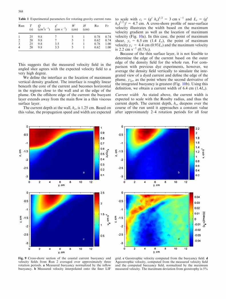
This suggests that the measured velocity field in theangled slice agrees with the expected velocity field to avery high degree.

We define the interface as the location of maximumvertical density gradient. The interface is roughly linearbeneath the core of the current and becomes horizontalin the regions close to the wall and at the edge of theplume. On the offshore edge of the current the buoyantlayer extends away from the main flow in a thin viscoussurface layer.

The current depth at the wall, ho, is 1.25 cm. Based onthis value, the propagation speed and width are expected

to scale with ci = (g¢ ho)1/2 = 3 cm s�1 and Lr = (g¢

ho)1/2/f = 4.7 cm. A cross-shore profile of near-surface

velocity illustrates the width based on the maximumvelocity gradient as well as the location of maximumvelocity (Fig. 10a). In this case, the point of maximumshear, ys = 6.5 cm (1.4 Lr), the point of maximumvelocity yv = 4.4 cm (0.93Lr) and the maximum velocityis 2.2 cm s�1 (0.73ci).

Because of the thin surface layer, it is not feasible todetermine the edge of the current based on the outeredge of the density field for the whole run. For com-parison with previous dye experiments, however, weaverage the density field vertically to simulate the inte-grated view of a dyed current and define the edge of theplume, y2q, as the point where the second derivative ofthe integrated buoyancy is greatest (Fig. 10b). Using thisdefinition, we obtain a current width of 6.4 cm (1.4Lr).

Current width As stated above, the current width isexpected to scale with the Rossby radius, and thus thecurrent depth. The current depth, ho, deepens over thecourse of the run until it approaches a constant valueafter approximately 2–4 rotation periods for all four

Table 1 Experimental parameters for rotating gravity current runs

Run T(s)

Q(cm3s�1)

g¢(cm s�2)

W(cm)

H(cm)

Ro Fr

1 25 9.8 7 5 1 0.78 0.742 20 9.8 7 5 1 0.62 0.743 25 9.8 3.5 5 1 0.78 1.004 20 9.8 3.5 5 1 0.62 1.00

Fig. 9 Cross-shore section of the coastal current buoyancy andvelocity fields from Run 2 averaged over approximately threerotation periods. a Measured buoyancy normalized by the inflowbuoyancy. b Measured velocity interpolated onto the finer LIF

grid. c Geostrophic velocity computed from the buoyancy field. dAgeostrophic velocity, computed from the measured velocity fieldand the computed buoyancy field, normalized by the maximummeasured velocity. The maximum deviation from geostrophy is 5%

568

runs (Fig. 11). The higher g¢ runs reach the steady depthearlier than the lower g¢ runs, presumably because ci ishigher and thus information propagates more quickly.We define a steady depth, ho; for each run as the averagevalue between 4 and 7 rotation periods and compute acorresponding Rossby radius, Lr; and gravity currentpropagation speed, ci: The current width, as measuredby either ys or y2q and normalized by the steady Rossby

radius, widens during the first four rotation periods andthen levels off to a constant value (Figs. 12, 13). Theaverage value of the steady width is ð1:23� 0:14ÞLr andð1:28� 0:13ÞLr for ys and y2q, respectively. This valuefor ys is much greater than the value of 0:42Lr measuredby Stern et al. (1982). We expect that this is because theywere only able to measure the current width close to thenose of the current and thus did not measure the equi-librium width. The value that we obtain for the currentwidth, y2q, agrees well with the Griffiths and Hopfinger(1983) value of 1:4Lr: Since we calculate the width basedon curvature in the vertically averaged density profile, itis not surprising that our value is slightly lower thantheirs, which is based on the maximum offshore extent ofthe dye.

Current stability Both ys and y2q increase smoothlyduring the first four rotation periods for all four runs.For later time, however, the variability increasesnoticeably for both of the lower g¢ runs (Figs. 12, 13;grey circles). This is probably indicative of instabilityalong the front. Four rotation periods corresponds withthe time when the current has widened to approximatelyy ¼ Lr: This is consistent with Griffiths and Linden(1981), who found that the unstable current width was afunction of Lr:

Current speed When the nose of the current first arrivesin the measurement section (1 < t/T < 2), the maxi-mum velocity is equal to ci (Fig. 14). Subsequently, themaximum speed decays exponentially and is relativelyconstant after four rotation periods. The average valueof the steady velocity maximum is (0.74 ± 0.09)ci.

0 1 2 30

2

4

6

8

10

12

u, cm/s

y, c

ma

0 0.5 10

2

4

6

8

10

12

C/Cmax

b

Fig. 10 Cross-shore profiles of surface velocity (a) and depthaveraged buoyancy (b). The solid and open circles in a mark thelocation of maximum velocity and shear. The solid and open circlesin b mark the location of maximum first and second derivatives inthe integrated buoyancy. The buoyancy has been normalized by thelocal maximum for plotting

1 2 3 4 5 6 7 80

1

2

3

4

5

h o, cm

t/T

g’ = 6.9cm s–1, T=25sg’ = 6.9cm s–1, T=20sg’ = 3.5cm s–1, T=25sg’ = 3.5cm s–1, T=20s

Fig. 11 Coastal current depthat the wall, ho for all four runs

1 2 3 4 5 6 7 80

1

2

3

4

y s/Lr

t/T

g’ = 6.9cm s–1, T=25sg’ = 6.9cm s–1, T=20sg’ = 3.5cm s–1, T=25sg’ = 3.5cm s–1, T=20s

Fig. 12 Location of maximumshear normalized by the Rossbyradius in the coastal current forall four runs

569

Lentz and Helfrich (2002), Griffiths and Hopfinger(1983) and Stern et al. (1982) all observe a decay inthe nose speed and an increase in the current width.Lentz and Helfrich (2002) show that the nose speeddecays as t�1/2 and the current width increases as t1/2,which is consistent with the observations in the twoother studies. They hypothesize that the temporalevolution of the current is due to viscous interfacialdrag between the buoyant current and the ambientfluid. The t�1/2 and t1/2 dependence for the velocityand width of the current qualitatively describes theevolution that we observe in the first 1–4 rotationsperiods. However, the width and speed appear to besteady after that. This indicates that, while interfacialdrag and offshore Ekman transport continue to beimportant, the coastal current may achieve a cross-shore balance.

Transport Finally, since we can calculate the transportdirectly, it is useful to compare it to the scaling forgeostrophic transport, Qg ¼ ðg0h2oÞ=2f (Fong and Geyer2002; Lentz and Helfrich 2002). The transport ofbuoyant water is calculated in the same fashion as forthe non-rotating experiments. The data are filtered witha Butterworth filter that has a filter width equal to therotation period. Qg is a reasonably good estimate of thealong-shore transport of buoyant fluid (Fig. 15). Notethat in our experiments, the measurement location is54 cm downstream of the source and so the transport atthat location will be subject to a lag due to the advectivetravel time of the current. The estimate is very sensitiveto the depth, ho. The depth measurement depends on thelocation of the water surface in the image, which can bea somewhat noisy measurement. We expect that thiserror explains the variation in the transport estimates.

1 2 3 4 5 6 7 80

1

2

3

4

y 2ρ/L

r

t/T

g’ = 6.9cm s–1, T=25sg’ = 6.9cm s–1, T=20sg’ = 3.5cm s–1, T=25sg’ = 3.5cm s–1, T=20s

Fig. 13 Location of theoffshore plume frontnormalized by the Rossbyradius in the coastal current forall four runs. The front isdefined as the maximum in thesecond derivative of thevertically averaged buoyancy

1 2 3 4 5 6 7 80

0.5

1

1.5

2

u max

/ci

t/T

g’ = 6.9cm s–1, T=25sg’ = 6.9cm s–1, T=20sg’ = 3.5cm s–1, T=25sg’ = 3.5cm s–1, T=20s

Fig. 14 Maximum velocitynormalized by the propagationspeed in the coastal current forall four runs

1 2 3 4 5 6 7 80

1

2

3

g’h o2 /2

fQ

t/T

g’ = 6.9cm s–1, T=25sg’ = 6.9cm s–1, T=20sg’ = 3.5cm s–1, T=25sg’ = 3.5cm s–1, T=20s

Fig. 15 Normalizedgeostrophic estimate ofalongshore transport ðg0h2

o=2f Þ

570

5 Conclusions

Velocity and density are measured simultaneously in thecross-section of a rotating buoyant gravity current usingPIV–PLIF. The implementation of the PIV–PLIF tech-nique described in the current work involves two newmodifications. The first is to adapt the existing techniquefor use on a rotating table. The second modificationallows the transport in a buoyant current to be measureddirectly. This involves rotating the measurement plane15� from the horizontal so that the entire cross-section iscaptured, but particle displacements are still resolved.The two acquired fields are used to calculate theinstantaneous transport of buoyant fluid through thecross-section. The technique is successful in measuringthe transport in a non-rotating channel to within 5% ofthe prescribed flow rate.

The measurement technique is subsequently appliedto a buoyant rotating gravity current. After the currentarrives at the measurement area, it is observed to dee-pen, widen and slow for 1–3 rotation periods and thenlevel off to a constant depth, width and speed for theremaining 4 rotation periods of the run. A gravity cur-rent propagation speed, ci; and a Rossby radius, Lr; aredefined based on the steady depth achieved at the end ofthe run. The maximum velocity in the current is equal toci near the nose and decays to a steady value of0:74� 0:09ci: The steady widths of the current, mea-sured according to the location of maximum velocityshear and the offshore inflection point in the densityprofile, are 1:23� 0:14Lr and 1:28� 0:13Lr; respectively.These agree with the width reported by Griffiths andHopfinger (1983). The geostrophic scaling,Qfw ¼ ðg0h2

oÞ=2f ; is relatively successful at predicting thetransport in the coastal current, but may be sensitive toerrors associated with determining the current depthexactly.

Direct calculation of the geostrophic velocity fieldusing the measured density field agrees with the mea-sured velocity field to within 5–10%. Furthermore, theobserved deviations from geostrophy are concentratednear the edges of the current, where viscous diffusion ofmomentum is expected to be significant. This agreement,in addition to the results in the non-rotating channel,confirm that the technique is accurate and capable ofhigh resolution measurement.

It is important to note that the angled slice techniqueis expected to be susceptible to significant out-of-planeerrors in highly turbulent or three dimensional flows.The limits of its applicability have not been tested here,but it is expected to yield accurate results for a broadclass of laboratory flows.

Acknowledgments The author would like to thank M. Brennan forsuggesting the angled laser sheet, and S. Monismith, D. Fong, C.Troy, E. Cowen and J. Crimaldi for support in the developmentand implementation of the experiments. This research was sup-ported by NSF grant OCE-0118029.

References

Alahyari A, Longmire E (1994) Particle image velocimetry in avariable-density flow: application to a dynamically evolvingmicroburst. Exp Fluids 17(6):434–440

Avicola G, Huq P (2002) Scaling analysis for the interaction be-tween a buoyant coastal current and the continental shelf:experiments and observations. J Phys Oceanogr 32(11):3233–3248

Borg A, Bolinder J, Fuchs L (2001) Simultaneous velocity andconcentration measurements in the near field of a turbulentlow-pressure jet by digital particle inmage velocimetry-planarlaser-induced fluorescence. Exp Fluids 31:140–152

Condie S, Ivey G (1988) Convectively driven coastal currents in arotating basin. J Mar Res 46(3):473–494

Cowen E, Monismith S (1997) A hybrid digital particle trackingvelocimetry technique. Exp Fluids 22(3):199–211

Cowen E, Chang KA, Liao Q (2001) A single camera coupledPTV–LIF technique. Exp Fluids 31(1):63–73

Crimaldi J (1997) The effect of photobleaching and velocity fluc-tuations on single-point LIF measurements. Exp Fluids23(4):325–330

Crimaldi J, Koseff J (2001) High-resolution measurements of thespatial and temporal structure of a turbulent plume. Exp Fluids31:90–102

Fong D, Geyer W (2002) The alongshore transport of fresh waterin a surface-trapped river plume. J Phys Oceanogr 32(3):957–972

Griffiths R (1986) Gravity currents in rotating systems. Annu RevFluid Mech 18:59–89

Griffiths R, Hopfinger E (1983) Gravity currents moving along alateral boundary in a rotating fluid. J Fluid Mech 134:357–399

Griffiths R, Linden P (1981) The stability of buoyancy-drivencoastal currents. Dyn Atmos Oceans 5(4):281–306

Horner-Devine A, Fong D, Monismith S, Maxworthy T (2006)Laboratory experiments simulating a coastal river inflow. JFluid Mech 555:203–232

Law AK, Wang H, Herlina (2003) Combined particle image ve-locimetry/planar laser induced fluorescence for integral model-ing of buoyant jets. J Eng Mech 129(10):1189–1196

Lentz S, Helfrich K (2002) Buoyant gravity currents along asloping bottom in a rotating fluid. J Fluid Mech 464:251–278

Liao Q, Cowen E (2005) An efficient anti-aliasing spectral contin-uous window shifting technique for PIV. Exp Fluids 38(2):197–208

Lide D (2003) CRC handbook of chemistry and physics. CRCPress, Boca Raton

Lowe R, Linden P, Rottman J (2002) A laboratory study of thevelocity structure in an intrusive gravity current. J Fluid Mech456:33–48

Raffel M, Willert C, Kompenhans J (1998) Particle image veloci-metry. Springer, Berlin Heidelberg New York

Stern M, Whitehead J, Hua BL (1982) The intrusion of a densitycurrent along the coast of a rotating fluid. J Fluid Mech123:237–265

Sveen J, Cowen E (2004) Quantitative imaging techniques and theirapplication to wavy flow. In: J G, PLF L, GK P (eds) PIV andwater waves, vol 9. World Scientific, Singapore, pp 1–49

Troy C, Koseff J (2005) The generation and quantitative visuali-zation of breaking internal waves. Exp Fluids 38:549–562

Vinger A, McClimans T, Tryggestad S (1981) Laboratory obser-vations of instabilities in a straight coastal current. In: TheNorwegian Coastal Current, vol 2. University of Bergen, Nor-way, pp 553–582

Walker D (1987) A fluorescence technique for measurement ofconcentration in mixing liquids. J Phys E 20:217–224

571