veri ambarları ve olap - dr. sadi evren...

VeriAmbarlarıveOLAP

ŞadiEvrenŞEKER

YouTubeKanalı:BilgisayarKavramları

www.SadiEvrenSEKER.com

Kaynaklar•  DataMining:Concepts

andTechniques,ThirdEdi8on(TheMorganKaufmannSeriesinDataManagementSystems)3rdEdiEon

•  byJiaweiHan(Author),MichelineKamber(Author),JianPei(Author)

90’larveOLAP

•  VeriAmbarıTeknolojileri(OLAP’ailkgeçişlerveOLTP’lerdekizorluklardandolayıgeçiciveriambarlarıoluşturmafikri)

•  İhEyaçlar•  OnlineAnalyEcalProcessing•  OLTP:OnlineTransacEonProcessing

OLTPvsOLAP

OLTP OLAP Kullanıcılar clerk, IT professional knowledge worker

Fonksiyonlar day to day operations decision support

DB Tasarım application-oriented subject-oriented

Veri current, up-to-date detailed, flat relational isolated

historical, summarized, multidimensional integrated, consolidated

Kullanım repetitive ad-hoc

Erişim read/write index/hash on prim. key

lots of scans

İşlerin boyu short, simple transaction complex query

# records accessed tens millions

#users thousands hundreds

DB boyutu 100MB-GB 100GB-TB

Metrikler transaction throughput query throughput, response

İkiKavram•  OLTP–OnlineTransacEonProcessing

– Örneğin:Bankahesaplarındakihareketler,biletişlemleri

– GeneldeküçüktransacEonlar–  Verininküçükbirkısmıileilgili–  Sıkvesüreklitekrarlarşeklindeçalış]rılıyor

•  OLAP–OnlineAnalyEcalProcessing–  BüyüktransacEonlar–  Karmaşıksorgular– Dahabüyükveriyeerişim–  Sıkyapılmayansorgular

TemelKavramlar

•  YıldızŞeması(StarSchema)– FactTable:Sıkgüncellenen,çoğunluklaeklemeyapılan,vegeneldeçokbüyüktablolardır

– DimensionTable:Sıkgüncellenmeyen,çokbüyükolmayantablolar

Sa]şÜrünID

MüşteriIDÇalışanIDŞubeID

KaçtaneTarih

Müşteri

Şube

Ürün

Çalışan

Join

Filter

Group

Aggregate

Star Schema

7

time_key day day_of_the_week month quarter year

time

location_key street city state_or_province country

location

Sales Fact Table

time_key

item_key

branch_key

location_key

units_sold

dollars_sold

avg_sales Measures

item_key item_name brand type supplier_type

item

branch_key branch_name branch_type

branch

Snowflake Schema

8


time

location_key street city_key

location

Sales Fact Table

time_key

item_key

branch_key

location_key

units_sold

dollars_sold

avg_sales

Measures

item_key item_name brand type supplier_key

item


branch

supplier_key supplier_type

supplier

city_key city state_or_province country

city

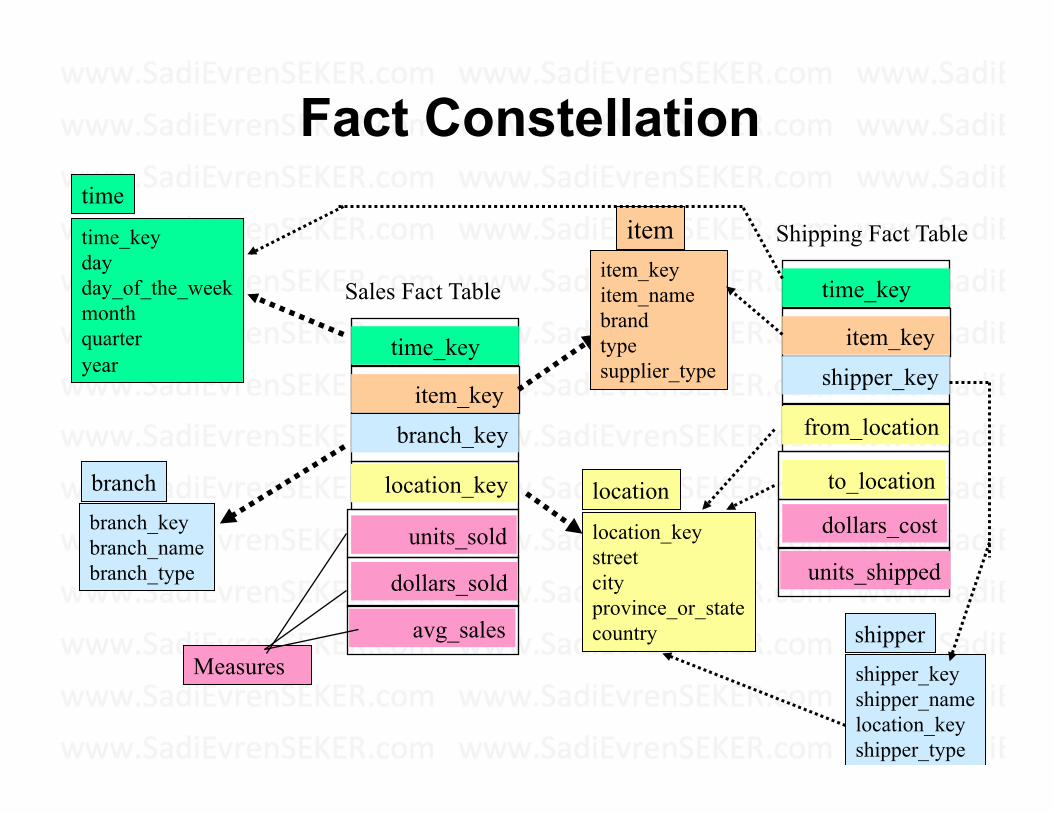
Fact Constellation

9


time

location_key street city province_or_state country

location

Sales Fact Table

time_key

item_key

branch_key

location_key

units_sold

dollars_sold

avg_sales Measures

item_key item_name brand type supplier_type

item


branch

Shipping Fact Table

time_key

item_key

shipper_key

from_location

to_location

dollars_cost

units_shipped

shipper_key shipper_name location_key shipper_type

shipper

StarSchema

•  Yavaş]r:Indeksoluşturulması,joinler,sorgularınözelolarakçalış]rılması

•  MaterializedView

VeriKüpleri(DataCube)

•  AslındaKüpDeğildirler

•  ÇokboyutluOLAP(mulEdimensionalOLAP)olarakdaisimlendirilirler

•  FactDatahücrelerdedurmaktadır

•  Slide,EdgeveCornerüzerindeaggregateddatatutulmaktadır

Ürü

nler

Aylar

Endüstri Bölge Yıllar Kategori Ülke Çeyrek Ürün Şehir Ay Hafta Şube Gün

Örnek Veri Küpü

Amerikadaki yıllık TV satışları

Tarih

Ülk

e

sum

sum TV

VCR PC

1Qtr 2Qtr 3Qtr 4Qtr U.S.A

Canada

Mexico

sum

BazıAggregateTakEkleri•  Dimensionaeributeşayetkeydeğilsegeneldeaggregateedilir

•  Distributive: if the result derived by applying the function to n aggregate values is the same as that derived by applying the function on all the data without partitioning

•  E.g., count(), sum(), min(), max() •  Algebraic: if it can be computed by an algebraic function with

M arguments (where M is a bounded integer), each of which is obtained by applying a distributive aggregate function

•  E.g., avg(), min_N(), standard_deviation() •  Holistic: if there is no constant bound on the storage size

needed to describe a subaggregate. •  E.g., median(), mode(), rank()

Cube: A Lattice of Cuboids

14

time,item

time,item,location

time, item, location, supplier

all

time item location supplier

time,location

time,supplier

item,location

item,supplier

location,supplier

time,item,supplier

time,location,supplier

item,location,supplier

0-D (apex) cuboid

1-D cuboids

2-D cuboids

3-D cuboids

4-D (base) cuboid

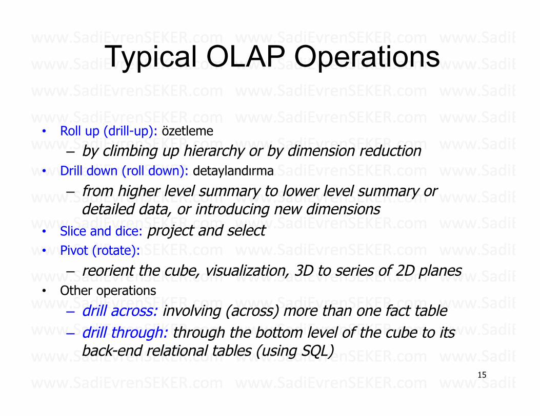
Typical OLAP Operations

•  Roll up (drill-up): özetleme

–  by climbing up hierarchy or by dimension reduction •  Drill down (roll down): detaylandırma

–  from higher level summary to lower level summary or detailed data, or introducing new dimensions

•  Slice and dice: project and select •  Pivot (rotate):

–  reorient the cube, visualization, 3D to series of 2D planes •  Other operations

–  drill across: involving (across) more than one fact table –  drill through: through the bottom level of the cube to its

back-end relational tables (using SQL) 15

16

Fig. 3.10 Typical OLAP Operations

A Star-Net Query Model

17

Shipping Method

AIR-EXPRESS

TRUCK ORDER

Customer Orders

CONTRACTS

Customer

Product

PRODUCT GROUP

PRODUCT LINE

PRODUCT ITEM

SALES PERSON

DISTRICT

DIVISION

Organization Promotion

CITY

COUNTRY

REGION

Location

DAILY QTRLY ANNUALY Time

Each circle is called a footprint

Browsing a Data Cube

•  Visualization •  OLAP capabilities •  Interactive manipulation

18

Chapter 4: Data Warehousing and On-line Analytical Processing

•  Data Warehouse: Basic Concepts

•  Data Warehouse Modeling: Data Cube and OLAP

•  Data Warehouse Design and Usage

•  Data Warehouse Implementation

•  Data Generalization by Attribute-Oriented Induction

•  Summary

19

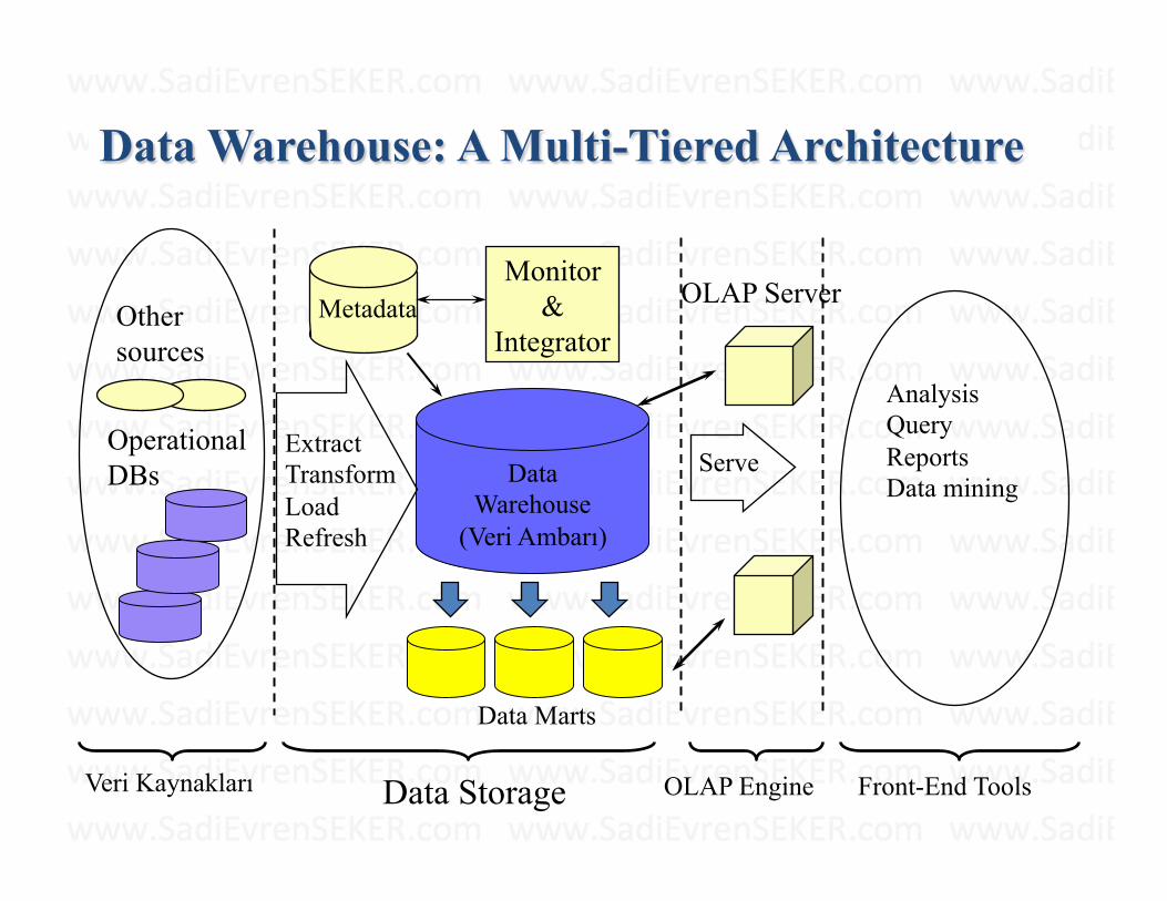
Data Warehouse: A Multi-Tiered Architecture

Data Warehouse

(Veri Ambarı)

Extract Transform Load Refresh

OLAP Engine

Analysis Query Reports Data mining

Monitor &

Integrator Metadata

Veri Kaynakları Front-End Tools

Serve

Data Marts

Operational DBs

Other sources

Data Storage

OLAP Server

Design of Data Warehouse: A Business Analysis Framework

•  Four views regarding the design of a data warehouse –  Top-down view

•  allows selection of the relevant information necessary for the data warehouse

–  Data source view •  exposes the information being captured, stored, and

managed by operational systems

–  Data warehouse view •  consists of fact tables and dimension tables

–  Business query view •  sees the perspectives of data in the warehouse from the view

of end-user

21

Data Warehouse Design Process

•  Top-down, bottom-up approaches or a combination of both –  Top-down: Starts with overall design and planning (mature) –  Bottom-up: Starts with experiments and prototypes (rapid)

•  From software engineering point of view –  Waterfall: structured and systematic analysis at each step before

proceeding to the next –  Spiral: rapid generation of increasingly functional systems, short turn

around time, quick turn around •  Typical data warehouse design process

–  Choose a business process to model, e.g., orders, invoices, etc. –  Choose the grain (atomic level of data) of the business process –  Choose the dimensions that will apply to each fact table record –  Choose the measure that will populate each fact table record

22

Data Warehouse Development: A

Recommended Approach

23 Define a high-level corporate data model

Data Mart

Data Mart

Distributed Data Marts

Multi-Tier Data Warehouse

Enterprise Data Warehouse

Model refinement Model refinement

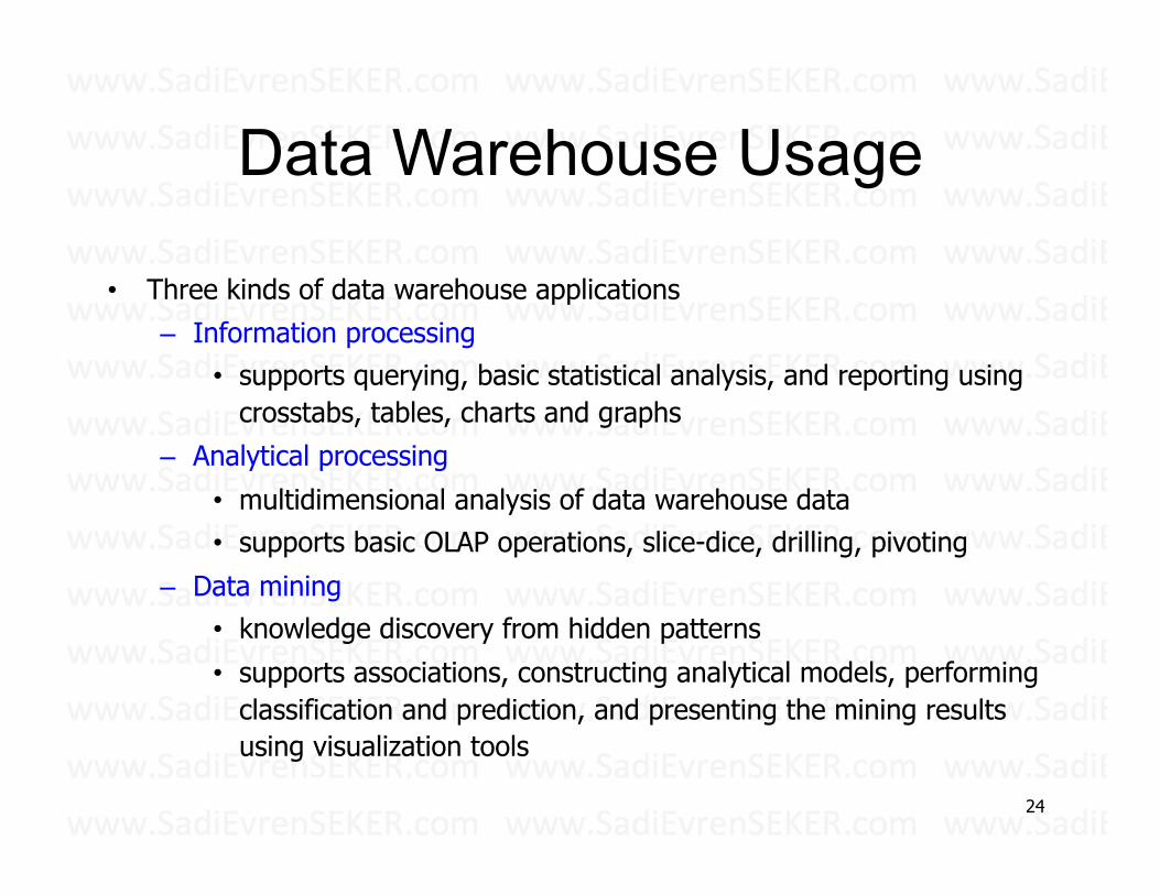
Data Warehouse Usage

•  Three kinds of data warehouse applications –  Information processing

•  supports querying, basic statistical analysis, and reporting using crosstabs, tables, charts and graphs

–  Analytical processing

•  multidimensional analysis of data warehouse data •  supports basic OLAP operations, slice-dice, drilling, pivoting

–  Data mining •  knowledge discovery from hidden patterns

•  supports associations, constructing analytical models, performing classification and prediction, and presenting the mining results using visualization tools

24

From On-Line Analytical Processing (OLAP) to On Line Analytical Mining (OLAM)

•  Why online analytical mining? –  High quality of data in data warehouses

•  DW contains integrated, consistent, cleaned data –  Available information processing structure surrounding

data warehouses •  ODBC, OLEDB, Web accessing, service facilities,

reporting and OLAP tools –  OLAP-based exploratory data analysis

•  Mining with drilling, dicing, pivoting, etc. –  On-line selection of data mining functions

•  Integration and swapping of multiple mining functions, algorithms, and tasks

25







•  Summary

26

Efficient Data Cube Computation

•  Data cube can be viewed as a lattice of cuboids –  The bottom-most cuboid is the base cuboid –  The top-most cuboid (apex) contains only one cell –  How many cuboids in an n-dimensional cube with L levels?

•  Materialization of data cube –  Materialize every (cuboid) (full materialization), none

(no materialization), or some (partial materialization)

–  Selection of which cuboids to materialize •  Based on size, sharing, access frequency, etc.

27

)11( +∏

==n

i iLT

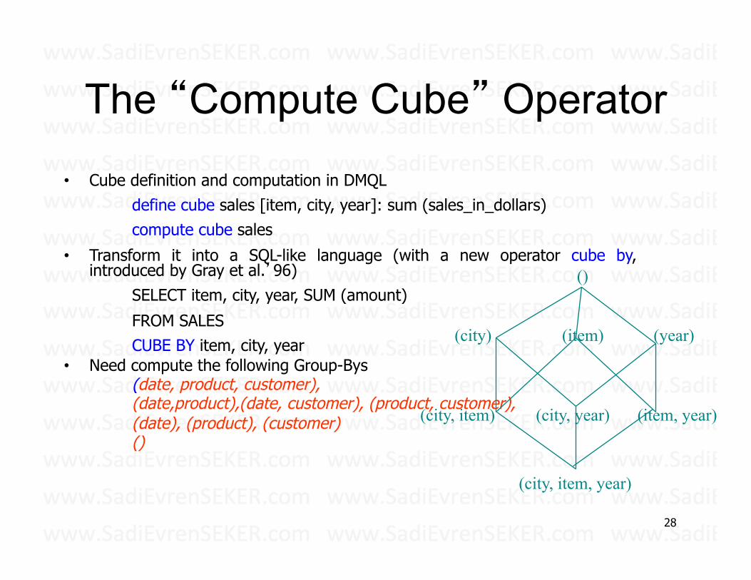
The “Compute Cube” Operator

•  Cube definition and computation in DMQL define cube sales [item, city, year]: sum (sales_in_dollars) compute cube sales

•  Transform it into a SQL-like language (with a new operator cube by, introduced by Gray et al.’96)

SELECT item, city, year, SUM (amount)

FROM SALES CUBE BY item, city, year

•  Need compute the following Group-Bys (date, product, customer), (date,product),(date, customer), (product, customer), (date), (product), (customer) ()

28

(item) (city)

()

(year)

(city, item) (city, year) (item, year)

(city, item, year)

Indexing OLAP Data: Bitmap Index

•  Index on a particular column •  Each value in the column has a bit vector: bit-op is fast •  The length of the bit vector: # of records in the base table •  The i-th bit is set if the i-th row of the base table has the value for the

indexed column •  not suitable for high cardinality domains –  A recent bit compression technique, Word-Aligned Hybrid (WAH), makes it

work for high cardinality domain as well [Wu, et al. TODS’06]

29

Cust Region TypeC1 Asia RetailC2 Europe DealerC3 Asia DealerC4 America RetailC5 Europe Dealer

RecID Retail Dealer1 1 02 0 13 0 14 1 05 0 1

RecIDAsia Europe America1 1 0 02 0 1 03 1 0 04 0 0 15 0 1 0

Base table Index on Region Index on Type

Indexing OLAP Data: Join Indices

•  Join index: JI(R-id, S-id) where R (R-id, …) ▹◃ S (S-id, …)

•  Traditional indices map the values to a list of record ids –  It materializes relational join in JI file and

speeds up relational join •  In data warehouses, join index relates the values

of the dimensions of a start schema to rows in the fact table. –  E.g. fact table: Sales and two dimensions city

and product •  A join index on city maintains for each

distinct city a list of R-IDs of the tuples recording the Sales in the city

–  Join indices can span multiple dimensions

30

Efficient Processing OLAP Queries

•  Determine which operations should be performed on the available cuboids

–  Transform drill, roll, etc. into corresponding SQL and/or OLAP operations, e.g.,

dice = selection + projection

•  Determine which materialized cuboid(s) should be selected for OLAP op.

–  Let the query to be processed be on {brand, province_or_state} with the condition “year = 2004”, and there are 4 materialized cuboids available:

1) {year, item_name, city}

2) {year, brand, country}

3) {year, brand, province_or_state}

4) {item_name, province_or_state} where year = 2004

Which should be selected to process the query?

•  Explore indexing structures and compressed vs. dense array structs in MOLAP 31

OLAP Server Architectures

•  Relational OLAP (ROLAP) –  Use relational or extended-relational DBMS to store and manage

warehouse data and OLAP middle ware –  Include optimization of DBMS backend, implementation of

aggregation navigation logic, and additional tools and services –  Greater scalability

•  Multidimensional OLAP (MOLAP) –  Sparse array-based multidimensional storage engine –  Fast indexing to pre-computed summarized data

•  Hybrid OLAP (HOLAP) (e.g., Microsoft SQLServer) –  Flexibility, e.g., low level: relational, high-level: array

•  Specialized SQL servers (e.g., Redbricks) –  Specialized support for SQL queries over star/snowflake schemas

32







•  Summary

33

Attribute-Oriented Induction

•  Proposed in 1989 (KDD ‘89 workshop) •  Not confined to categorical data nor particular measures

•  How it is done? –  Collect the task-relevant data (initial relation) using a

relational database query –  Perform generalization by attribute removal or attribute

generalization –  Apply aggregation by merging identical, generalized

tuples and accumulating their respective counts –  Interaction with users for knowledge presentation

34

Attribute-Oriented Induction: An Example

Example: Describe general characteristics of graduate students in the University database

•  Step 1. Fetch relevant set of data using an SQL statement, e.g.,

Select * (i.e., name, gender, major, birth_place, birth_date, residence, phone#, gpa)

from student where student_status in {“Msc”, “MBA”, “PhD” }

•  Step 2. Perform attribute-oriented induction •  Step 3. Present results in generalized relation, cross-tab,

or rule forms 35

Class Characterization: An Example

36

Name Gender Major Birth-Place Birth_date Residence Phone # GPAJimWoodman

M CS Vancouver,BC,Canada

8-12-76 3511 Main St.,Richmond

687-4598 3.67

ScottLachance

M CS Montreal, Que,Canada

28-7-75 345 1st Ave.,Richmond

253-9106 3.70

Laura Lee…

F…

Physics…

Seattle, WA, USA…

25-8-70…

125 Austin Ave.,Burnaby…

420-5232…

3.83…

Removed Retained Sci,Eng,Bus

Country Age range City Removed Excl,VG,..

Gender Major Birth_region Age_range Residence GPA Count M Science Canada 20-25 Richmond Very-good 16 F Science Foreign 25-30 Burnaby Excellent 22 … … … … … … …

Birth_Region

GenderCanada Foreign Total

M 16 14 30 F 10 22 32

Total 26 36 62

Prime Generalized Relation

Initial Relation

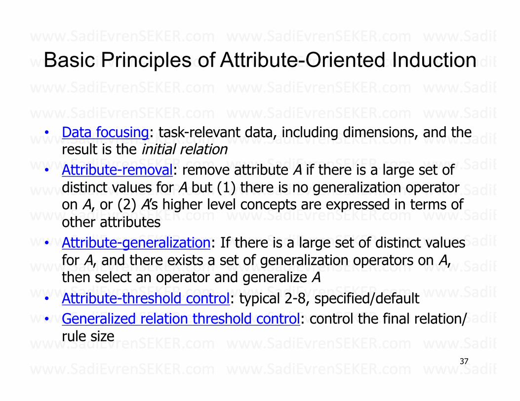
Basic Principles of Attribute-Oriented Induction

•  Data focusing: task-relevant data, including dimensions, and the result is the initial relation

•  Attribute-removal: remove attribute A if there is a large set of distinct values for A but (1) there is no generalization operator on A, or (2) A’s higher level concepts are expressed in terms of other attributes

•  Attribute-generalization: If there is a large set of distinct values for A, and there exists a set of generalization operators on A, then select an operator and generalize A

•  Attribute-threshold control: typical 2-8, specified/default •  Generalized relation threshold control: control the final relation/

rule size

37

Attribute-Oriented Induction: Basic Algorithm

•  InitialRel: Query processing of task-relevant data, deriving the initial relation.

•  PreGen: Based on the analysis of the number of distinct values in each attribute, determine generalization plan for each attribute: removal? or how high to generalize?

•  PrimeGen: Based on the PreGen plan, perform generalization to the right level to derive a “prime generalized relation”, accumulating the counts.

•  Presentation: User interaction: (1) adjust levels by drilling, (2) pivoting, (3) mapping into rules, cross tabs, visualization presentations.

38

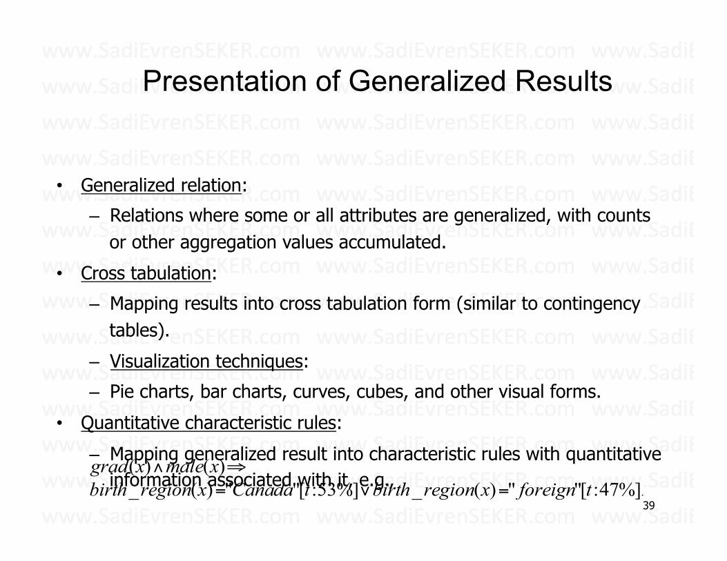
Presentation of Generalized Results

•  Generalized relation:

–  Relations where some or all attributes are generalized, with counts or other aggregation values accumulated.

•  Cross tabulation:

–  Mapping results into cross tabulation form (similar to contingency tables).

–  Visualization techniques:

–  Pie charts, bar charts, curves, cubes, and other visual forms.

•  Quantitative characteristic rules:

–  Mapping generalized result into characteristic rules with quantitative information associated with it, e.g.,

39 .%]47:["")(_%]53:["")(_

)()(tforeignxregionbirthtCanadaxregionbirth

xmalexgrad=∨=

⇒∧

Mining Class Comparisons

•  Comparison: Comparing two or more classes •  Method:

–  Partition the set of relevant data into the target class and the contrasting class(es)

–  Generalize both classes to the same high level concepts –  Compare tuples with the same high level descriptions –  Present for every tuple its description and two measures

•  support - distribution within single class •  comparison - distribution between classes

–  Highlight the tuples with strong discriminant features •  Relevance Analysis:

–  Find attributes (features) which best distinguish different classes 40

Concept Description vs. Cube-Based OLAP

•  Similarity: –  Data generalization –  Presentation of data summarization at multiple levels of

abstraction –  Interactive drilling, pivoting, slicing and dicing

•  Differences: –  OLAP has systematic preprocessing, query independent,

and can drill down to rather low level –  AOI has automated desired level allocation, and may

perform dimension relevance analysis/ranking when there are many relevant dimensions

–  AOI works on the data which are not in relational forms

41







•  Summary

42

Summary

•  Data warehousing: A multi-dimensional model of a data warehouse –  A data cube consists of dimensions & measures –  Star schema, snowflake schema, fact constellations –  OLAP operations: drilling, rolling, slicing, dicing and pivoting

•  Data Warehouse Architecture, Design, and Usage –  Multi-tiered architecture –  Business analysis design framework –  Information processing, analytical processing, data mining, OLAM (Online

Analytical Mining) •  Implementation: Efficient computation of data cubes

–  Partial vs. full vs. no materialization –  Indexing OALP data: Bitmap index and join index –  OLAP query processing –  OLAP servers: ROLAP, MOLAP, HOLAP

•  Data generalization: Attribute-oriented induction

43

References (I) •  S.Agarwal,R.Agrawal,P.M.Deshpande,A.Gupta,J.F.Naughton,R.Ramakrishnan,andS.

Sarawagi.OnthecomputaEonofmulEdimensionalaggregates.VLDB’96•  D.Agrawal,A.E.Abbadi,A.Singh,andT.Yurek.Efficientviewmaintenanceindata

warehouses.SIGMOD’97•  R.Agrawal,A.Gupta,andS.Sarawagi.ModelingmulEdimensionaldatabases.ICDE’97•  S.ChaudhuriandU.Dayal.AnoverviewofdatawarehousingandOLAPtechnology.ACM

SIGMODRecord,26:65-74,1997•  E.F.Codd,S.B.Codd,andC.T.Salley.Beyonddecisionsupport.ComputerWorld,27,July

1993.•  J.Gray,etal.Datacube:ArelaEonalaggregaEonoperatorgeneralizinggroup-by,cross-tab

andsub-totals.DataMiningandKnowledgeDiscovery,1:29-54,1997.•  A.GuptaandI.S.Mumick.MaterializedViews:Techniques,ImplementaEons,and

ApplicaEons.MITPress,1999.•  J.Han.Towardson-lineanalyEcalmininginlargedatabases.ACMSIGMODRecord,27:97-107,

1998.•  V.Harinarayan,A.Rajaraman,andJ.D.Ullman.ImplemenEngdatacubesefficiently.

SIGMOD’96•  J.Hellerstein,P.Haas,andH.Wang.OnlineaggregaEon.SIGMOD'97

44

References (II) •  C.Imhoff,N.Galemmo,andJ.G.Geiger.MasteringDataWarehouseDesign:RelaEonaland

DimensionalTechniques.JohnWiley,2003•  W.H.Inmon.BuildingtheDataWarehouse.JohnWiley,1996•  R.KimballandM.Ross.TheDataWarehouseToolkit:TheCompleteGuidetoDimensional

Modeling.2ed.JohnWiley,2002•  P.O’NeilandG.Graefe.MulE-tablejoinsthroughbitmappedjoinindices.SIGMODRecord,24:8–

11,Sept.1995.•  P.O'NeilandD.Quass.Improvedqueryperformancewithvariantindexes.SIGMOD'97•  Microsox.OLEDBforOLAPprogrammer'sreferenceversion1.0.Inhep://www.microsox.com/

data/oledb/olap,1998•  S.SarawagiandM.Stonebraker.EfficientorganizaEonoflargemulEdimensionalarrays.ICDE'94•  A.Shoshani.OLAPandstaEsEcaldatabases:SimilariEesanddifferences.PODS’00.•  D.Srivastava,S.Dar,H.V.Jagadish,andA.V.Levy.AnsweringquerieswithaggregaEonusing

views.VLDB'96•  P.Valduriez.Joinindices.ACMTrans.DatabaseSystems,12:218-246,1987.•  J.Widom.Researchproblemsindatawarehousing.CIKM’95•  K.Wu,E.Otoo,andA.Shoshani,OpEmalBitmapIndiceswithEfficientCompression,ACMTrans.

onDatabaseSystems(TODS),31(1):1-38,200645

veri ambarları ve olap - dr. sadi evren...

Documents