Vertex Representations and their Applications in Computer Graphics

Claudio Esperanca�

COPPE, Prog. Eng. SistemasUniversidade Federal do Rio de JaneiroCidade Universitaria, C.T., Sala H319Rio de Janeiro, RJ, 21945-970, Brazil

E-mail: esperanc@lcg.ufrj.br

Hanan Samet�

Computer Science Department andCenter for Automation Research and

Institute for Advanced Computer ScienceUniversity of Maryland at College Park

College Park, Maryland 20742E-mail: hjs@umiacs.umd.edu

March 30, 1998

Abstract

The vertex representation, a new data structure for representing and manipulating orthogonal objects,is presented. Both interiors and boundaries of regions are represented implicitly through the aid of asingle vertex which is the tip of an infinite cone. The cones are similar to halfspaces in a CSG represen-tation; however, unlike CSG, the representation of an object with the vertices is unique. Additionally,vertex representations deal with scalar fields and not solids. Algorithms are given for generating vertexrepresentation models for primitive solids, performing affine transformations, set-theoretic operations,and displaying vertex representation models. The algorithms assume that the vertices are stored in alist although they could also be stored using other representations (e.g., a point variant of a quadtree).The contribution of the work lies, in part, in the generality of the solutions obtained through the use ofrecursion to construct the representation in higher dimensions, as well as performing the operations onit. This is largely a result of the switch of the primitive unit to being a one-dimensional vertex list ratherthan a two-dimensional vertex list which was the original formulation of the representation. The vertexrepresentation models the same objects that are obtained through use of methods such as an array ofvoxels or octrees (i.e., objects with orthogonal faces). Its advantage is that it requires less space and unlikeoctrees its space requirements are not sensitive to translation. Moreover, it enables increasing the qualityof the approximation of objects by increasing the number of vertices that make up the model. In contrast,increasing the quality of the approximation in a array of voxels requires doubling the resolution whichmeans a significant increase in the space requirements. The algorithms are illustrated via screen shots.

Keywords: Shape representation, orthogonal polygons, vertex lists, constructive solid geometry (CSG),solid modeling.

�The support of Conselho Nacional de Desenvolvimento Cientıfico e Tecnologico (CNPq), Projeto GEOTEC 481007/96-2 is

gratefully acknowledged.�The support of the National Science Foundation under Grant IRI-9712715, the Department of Energy under Contract

DEFG0295ER25237 is gratefully acknowledged.

1 Introduction

There are many different techniques for representing objects in computer graphics applications (e.g., [6,10, 15, 14]). The objects can be represented either by their interiors or by their boundaries. Each of theserepresentations has its advantages and disadvantages. At times, a more compact representation is desired inwhich case techniques such as runlength encoding are applied.

In this paper we describe the vertex representation which represents both interiors and boundaries ofregions implicitly through the aid of a single vertex which is the tip of an infinite cone. The cones aresimilar to halfspaces in a CSG representation; however, unlike CSG, the representation of an object withthe vertices is unique. Also, the vertex representation aims at representing scalar fields, not solids. Themodeling of solids is achieved by regarding a solid as as a scalar field which maps the interior of the solidto 1 and the exterior to 0. The vertex representation was originally presented as an alternative model fortwo-dimensional data represented as lists of rectangles for VLSI applications [18]. Algorithms have beendevised for a number of vertex representation operations in two dimensions [18].

Our contribution here is in showing how the vertex representation can be extended to represent orthogonalobjects in arbitrary dimensions, and presenting a number of algorithms for operations that are useful incomputer graphics. In particular, we describe algorithms for generating vertex representation models forprimitive solids, performing affine transformations, set operations, and displaying vertex representationmodels. Our algorithms assume that the vertices are stored in a list although they could also be stored usingother representations (e.g., a point variant of a quadtree). We do not address these other representations inthis paper.

The contribution of our work is the generality of the solutions that we obtain through the use of recursionto construct the representation in higher dimensions, as well as performing the operations on it. This islargely a result of the switch of the primitive unit to being a one-dimensional vertex list rather than atwo-dimensional vertex list [18].

The vertex representation models the same objects that are obtained through use of spatial enumerationmethods such as an array of voxels or octrees [7] (i.e., objects with orthogonal faces). The vertex repre-sentation models the same objects that are obtained through use of methods such as an array of voxels oroctrees (i.e., objects with orthogonal faces). Its advantage is that it requires less space and unlike octreesits space requirements are not sensitive to translation. Moreover, it enables increasing the quality of theapproximation of objects by increasing the number of vertices that make up the model. In contrast, increas-ing the quality of the approximation in a array of voxels requires doubling the resolution which means asignificant increase in the space requirements. i

The rest of this paper is organized as follows. Section 2 motivates the paper by reviewing a number ofobject representations, shows their strengths and weaknesses, and concludes with a brief explanation of howthe latter can be overcome by the vertex representation. This section can be skipped by readers who do notneed such a motivation. Section 3 reviews the vertex representation, while Section 4 presents some of itskey properties. Section 5 describes the organization of the elements of the vertex representation by meansof lists (termed vertex lists). This section also includes descriptions of a number of elementary operationsthat are used in the implementation of a number of solid modeling operations in Section 6. Concludingremarks are drawn in Section 7.

2 Object Representations

A common representation of the objects and their environment, and the one we focus on in this paper, isas a collection of cells (termed pixels and voxels in two and three dimensions, respectively) all of whoseboundaries (with dimensionality one less than that of the cells) are of unit size. In the applications that

1

we consider, the boundaries (i.e., edges and faces in two and three dimensions and higher, respectively) ofthe cells are orthogonal to each other and parallel to the coordinate axes. The elements of each collection(i.e., the cells) are labeled with values or attributes corresponding to the different objects and are frequentlyaggregated into subcollections of identically-valued cells. The shape of an object � can be represented eitherby the interiors of the cells comprising � , or by the subset of the boundaries of those cells comprising � thatare adjacent to the boundary of � .

Interior-based representations aggregate identically-valued cells by recording their locations. Thedrawback is the amount of space needed. This is alleviated by aggregating similarly-valued unit-sizedcells into blocks which are usually rectangular with sides that are parallel to the coordinate axes. Regionquadtrees [4] and region octrees [7] are examples of such representations for two and three-dimensional data(variants for data of higher dimension also exist), respectively, that recursively decompose the environmentcontaining the objects into four or eight, respectively, rectangular congruent blocks until each block is eithercompletely occupied by an object or is empty. The drawback of region quadtrees and octrees is that theirspace requirements depend on their position and hence they are sensitive to translation. Interior-basedrepresentations are good for computing volume as well as determining whether or not a point is inside oroutside the object.

On the other hand, boundary-based representations are more amenable to the calculation of propertiespertaining to shape (e.g., perimeter, extent, etc.). In this case, we simply record the location of the differentboundary elements associated with each cell of each object and their nature (i.e., their orientation and thelocations of the cells to which they are adjacent). For example, in two dimensions, the boundary elementsare just the sides of the cells (i.e., unit vectors), while in three dimensions, the boundary elements are thefaces of the cells (i.e., squares of unit area with a direction equal to the normal to the object). Boundary-based representations aggregate identically-valued cells whose boundary elements have the same direction,rather than just identically-valued cells as done by interior-based representations. In two dimensions, theaggregation yields boundary elements which are vectors whose length can be more than one.

Whichever boundary-based representation is used and regardless of whether any aggregation takes place,the representation must also enable the determination of the connectivity between individual boundaryelements. The connectivity may be implicit or explicit (e.g., by specifying which boundary elements areconnected). As an example of a boundary-based representation, let us consider two-dimensional objects inwhich case the boundary elements are vectors. The location of the vector is given by its start and end vertices.An object � has one more boundary than it has holes. Connectivity may be determined implicitly by orderingthe boundary elements ����� � of boundary ��� of � so that the end vertex of the vector � corresponding to ����� � isthe start vertex of the vector � � 1 corresponding to � ��� ��� 1. In dimensions higher than two, the relationshipbetween the boundary elements associated with a particular object is more complex, as is its expression.Whereas in two dimensions we just have one type of a boundary element (i.e., an edge or a vector consistingof two vertices), in ��� 2 dimensions, we have ��� 1 different boundary elements (e.g., faces and edgesin three dimensions). As we saw, in two dimensions, the ordered sequence of vectors is equivalent to animplicit specification of the boundary by virtue of the fact that each boundary element of an object can onlybe adjacent to two other elements. Thus consecutive boundary elements in the representation are implicitlyconnected. Implicit connectivity is not possible in ��� 2 dimensions as there are 2 ��� 1 different adjacencies(i.e., types of connectivities) per boundary element.

Nevertheless, in higher dimensions we do have a choice between an explicit and an implicit boundary-based representation. The boundary model (also known as BRep [1, 15]) is an example of an explicitboundary-based representation. Observe that in three dimensions, the boundary of an object is decomposedinto a set of faces, edges, and vertices. The result is an explicit model based on a combined geometric andtopological description of the object. The topology is captured by a set of relations that indicate explicitlyhow the faces, edges, and vertices are connected to each other. The drawback is that we need to update the

2

connectivity information after a series of operations.

Constructive Solid Geometry (CSG) [11] is an example of an interior-based representation that isapplicable to objects of arbitrary dimensionality. In this case, primitive instances of objects are combinedto form more complex objects by use of geometric transformations and regularized Boolean set operations(e.g., union, intersection). When the primitive instances are halfspaces, the result is an boundary-basedrepresentation. In this case, the boundary of a � -dimensional object � consists of a collection of hyperplanesin � -dimensional space (i.e., the infinite boundaries of regions defined by the inequality � ���� 0 � ��� ��� 0where � 0 � 1). We have one halfspace for each � � 1 -dimensional boundary element of � .

Both of these representations (i.e., primitive instances of objects and halfspaces) are implicit becausethe object is determined by associating a set of regular Boolean set operations with the collection ofprimitive instances (which may be halfspaces) the result of which is the object � . Although both BRepand CSG are quite general, it is easy to constrain them to handle orthogonal objects. The drawback ofthese representations is that they are not unique. At times, some operations are more easily computed byconversion to interior-based representations (e.g., [16]).

Some interior-based and boundary-based representations can be made more compact by making use ofan ordering on the data (i.e., the cells, blocks, boundary elements, etc.) that it records (if one exists). Inparticular, instead of just recording the actual values of the cells and/or the actual locations of the cells,it records the change in the values of the cells and/or the locations of the cells where the value changes.The ordering is used to reconstruct the original association of values with their locations whenever we wishto determine what value is associated with a particular location. Although the reconstruction process is acostly one as it requires traversing the entire representation (i.e., all the objects), this is not a necessarily aproblem when execution of the operations inherently requires that the entire representation be traversed (e.g.,Boolean set operations, data structure conversion, erosion, dilation, etc.). On the other hand, operationswhich require the ability to randomly access a cell in the representation (e.g., neighbor finding) are inefficientin this case unless an additional access structure is imposed on the compact representation.

Runlength encoding [13] is an example of a method that can be applied to make an interior-basedrepresentation such as the array more compact. The actual locations of the cells are not recorded. Instead,it aggregates contiguous identically-valued cells into one-dimensional rectangles for which only the valueassociated with the cells comprising the rectangle and the length of the rectangle are recorded. The one-dimensional rectangles are ordered in raster-scan order which means that row 1 is followed by row 2, etc.The same technique is applicable to higher dimensional data in which case the one-dimensional rectanglesare ordered in terms of the rows, planes, etc. Given the location of any cell � in one-dimensional rectangle� , the value associated with � can be computed by referring to the location of the starting position of theentire representation and accumulating the lengths of the one-dimensional rectangles encountered before� . Interestingly, quadtrees and octrees can also be viewed as applications of runlength encoding to formaggregates in higher dimensions.

The same principles used in adapting runlength encoding to interior-based representations can also beused to a limited extent with some boundary-based representations. For example, in two dimensions, acommon boundary-based representation is the chain code [3] which indicates the relative locations of thecells that comprise the boundary of object � . In particular, it specifies the direction of each boundary elementand the number of adjacent unit-sized cells that make up the boundary element. Given the location of thefirst cell in the sequence corresponding to the boundary of � , we can determine the boundary of � by justfollowing the direction of the associated boundary element. Thus there is no need for the actual cells ortheir locations, as now � is uniquely identified. Therefore, in the chain code, the locations of the boundaryelements (i.e., the cells that are adjacent to them) are given implicitly while the nature of the boundaryelements is given explicitly (i.e., the direction of the boundary element). Each object has a separate chaincode.

3

Unfortunately, as we mentioned earlier, the chain code cannot be used for data in higher dimensionsthan two for the same reasons that the polygon representation could not be used. The problem is that theboundary elements are hyperplanes whose dimension is one less than the space in which they are embedded,and no natural order for traversing them exists. Thus we must turn to other solutions such as those basedon the vertex representation that are described in greater detail in the remaining sections. For the moment,we complete our discussion of the various object representations by giving a brief overview of the salientproperties of the vertex representation.

The vertex representation is based on the vertex algebra which was proposed by Shechtman [18] forstoring and processing VLSI masks. The vertex representation applies techniques similar to that of runlengthencoding to a orthogonal objects that are represented using blocks of arbitrary size and at arbitrary positions.Space is decomposed into multidimensional blocks (not necessarily disjoint) which are aggregated usingtechniques such as CSG by attaching weights that serve an analogous role to that of regularized union andset-difference. Instead of using combining elements that are blocks of finite area or halfspaces, it makes useof vertices which serve as tips of infinite cones.

Each cone is equivalent to an unbounded object formed by the intersection of � orthogonal halfspacesthat are parallel to the � coordinate axes passing through the vertex. In a sense, our representation resemblesCSG where the primitive elements are halfspaces. In particular, the vertex plays the role of a CSG primitiveand the region that it represents is equivalent to the intersection of the halfspaces that pass through it.However, unlike CSG, the representation of an object with the vertices is unique. The vertices have signsassociated with them indicating whether the space spanned by their cones are included or excluded fromthe object being modeled. The cones corresponding to the vertices are like infinite blocks thereby slightlyresembling a region octree. However, unlike the region octree, since they need not be disjoint, they areinvariant under translation.

3 Vertex Representations

A vertex is merely a point in space to which a scalar value (termed weight) is attached. A vertex representationis a set of vertices on which the following restrictions are imposed:

1. No two vertices may lie at the same point in space.

2. No vertices may have zero weight.

The modeling space1 of vertex representations are scalar fields, that is, functions that map each point ofa given � -dimensional space to a scalar value.

A null vertex representation (an empty set) represents a null scalar field by definition, i.e., a scalar fieldwhere all points are mapped to zero. Now consider a set containing only one vertex placed at point� with weight � . The effect of on the otherwise null field is to add � to all points � such that� ���� . The relationship denoted by ‘ � ’ is defined in the following manner: Let � 1 , � 2 ... � � be the � coordinate values of a point � , and let � 1, � 2 ... � � be the � coordinate values of a point � . Then,� ���� if and only if for all � � 1 ����� � , � � ����� . We may visualize the region in space that a vertex placed at � influences by imagining a flat-faced cone having its tip at � . Figure 1 depicts such a conein three-dimensional space.

As more vertices are added to the representation, the scalar field is modified accordingly. If we considera representation consisting of � vertices 1 � 2 ��� � �� , where the position of vertex � is denoted by � �

1Here we use a term defined by Requicha[10] in the context of solid modeling, despite the fact that the objects modeled viavertex representations are not rigid solids.

4

p(v)

x

y

z

Figure 1: Cone of a vertex placed at point � in � 3.

and its weight by � � , then the value of the corresponding scalar field ��� at a point � is given by

� � � � ������ ����� � �

Although the definition of vertex representations is complete at this point, it is rather difficult to visualizethe process of building a representation which approximates any given scalar field. Perhaps the most usefulinsight in this matter is to observe how vertex representations behave in spaces of increasing dimensions.Consider the task of building a vertex representation for a field that maps all points to 0, except those insidea given hyperrectangle which are mapped to 1.

We start by analyzing the one-dimensional case, where the rectangle is actually an interval defined bytwo endpoints � and � . Formally, given an interval � 1 � � � � , we wish to build a scalar field ��� 1 definedas

��� 1 � ��

1 if ��� � � �0 otherwise.

The solution is trivial enough and consists of a representation with two vertices: one at position �and weight � 1, and another at position � and weight � 1 (see Figure 2). Observe that this is only anapproximation of the desired field, since the field induced by the representation maps point � to 1 and notto 0.

a b

+10 01 -1

x

Figure 2: Vertex representation of a rectangle in one dimension.

Let us now step into the analogous two-dimensional problem. A two-dimensional axes-aligned rectangle( � 2)can be defined by two extreme points � and � . In other words, we wish to build a representation for ascalar field defined by

��� 2 � ��

1 if � 1 � � 1 � � 1 � � 2 � � 2 � � 2

0 otherwise.

The vertex representation obtained for the one-dimensional problem provides one half of the answerto the problem in two dimensions. By adding a second coordinate value equal to � 2 to each of those twovertices we obtain a rectangle that extends from � 2 to infinity in the positive direction of the � axis (seeFigure 3(a)). All that remains is to add two more vertices at � 1 � � 2 and � 1 � � 2 with weights � 1 and � 1,respectively (see Figure 3(b)).

5

a1

a2

b1

+1

0

0

1

-1

x

y

a1

a2

b1

b2

+1

+1

0

0

1

-1

-1

x

y

(a) (b)

Figure 3: A rectangle in 2 dimensions is produced by embedding a one-dimensional rectangle in two-dimensional space (a) and “closing” it with asecond one-dimensional rectangle (b).

The solution to the general problem of building a vertex representation for a hyperrectangle in �dimensions can then be seen as a recursive process. If � is 1, the solution is as described earlier. Otherwise:

1. Build a vertex representation for a ��� 1-dimensional rectangle obtained by discarding the last coor-dinate values of the extreme points, say, � � and � � .

2. Make two copies of the vertex representation obtained in (1). Set the ����

coordinate value of allvertices of the first copy to � � and those of the second copy to � � . Switch the weights of the verticesof the second copy from � 1 to � 1 and vice-versa.

Although simple-minded, the examples above illustrate a general way of processing vertex representa-tions. In a nutshell, vertex representations defined in � -dimensional space can be processed by combiningvertex representations in � � 1-dimensional space. This general method of processing geometric structuresis known as the plane-sweep paradigm [9]. We shall return to this subject in Section 5.

4 Properties of Vertex Representations

Vertices, as defined in Section 3, define a vector space. We shall not give here a mathematical treatment ofthis matter, but it is useful to enumerate a few properties of vertex representations. In the discussion thatfollows, � and

�are scalar values, � and are vertices, � � is the field induced by , � is the position of

and � is the weight of .

Scalar multiplication: Multiplication of a vertex by a scalar � , written ��� means a vertex with thesame position as and weight equal to ��� � . The effect of this operation is a field which maps all pointsin the cone of to ��� � . Formally, ��� � � � � � � .Vertex addition: Adding two vertices � and , written � � is tantamount to putting them in the samerepresentation. The field produced by � � is the sum of the fields produced by � and individually.Formally, ��� � � � ��� � � � .Uniqueness of vertex representations: Vertex representations are unique in the sense that either a givenfield � can be represented by exactly one set of vertices or it cannot be represented by vertices at all.Uniqueness is ensured by the restrictions outlined in Section 3.

6

Boundary property: Loosely speaking, this property means that the vertex representation of a field �will be constituted solely of vertices placed at points where there is a change in the value of the field, thatis, at points on the boundary of the field. To put it another way, if all points in the neighborhood of a givenpoint � are mapped to the same scalar � , then no vertex exists at � . The rectangle example of Section 3demonstrate this property, as we can see that vertices needed to be placed only at the corners of the rectangle.

5 Vertex Lists

A convenient way of organizing the vertices of a representation is by means of lists. A list data structurerequires that its elements be linked together in some order. Since vertex representations naturally lendthemselves to be processed one dimension at a time, it is a good idea to maintain vertices sorted according tothe order in which a sweeping plane would encounter them. This means that a vertex list in one dimensionhas vertices sorted by their � coordinate values. Similarly, the vertices of a two-dimensional vertex list aresorted primarily with respect to their � coordinate values with ties broken by taking their � coordinate valuesinto account. In general, the vertices of a list in � dimensions are sorted primarily by their � �

�coordinate

values, while coordinates � � 1, � � 2 and so on act as secondary keys, tertiary keys etc. The fact that twovertices in the same representation cannot lie at the same position in space ensures that this scheme imposesa total ordering among the vertices of a list.

Let us return to the problem of building a vertex representation for a hyperrectangle in three dimensions.As seen in Section 3, an algorithm to perform this task with vertex lists would start by creating a one-dimensional vertex list, say � 1, with vertices placed along the � axis. A two-dimensional vertex list � 2would then be created by concatenating two slightly modified copies of � 1 placed at two different positionsalong the � axis. Finally, a three-dimensional vertex list � 3 would be created by concatenating two modifiedcopies of � 2 placed at two different positions along the � axis. This process is illustrated in Figure 4.

+1 +1

-1

+1 +1

-1

-1 -1

+1

-1 -1

+1

+1a1a1

a1

a1

a2a2 a3

a3

a3

a3

b3

b3

b3

b3

a2

a2 a2

a2

b2b2

b2

b2 b2

b2

a1a1

a1

-1b1 b1 b1

b1

b1 b1

b1

L1 L2 L3

} } }}

}}

Vertex

Position Weight

Figure 4: Building a vertex list for a three-dimensional rectangle by copyingand concatenating vertex lists of lower dimensions

7

5.1 Elementary vertex list operations

The processing of vertex list models usually follows the same approach employed in the hyperrectangleproblem. We will use the term recursive plane sweep to refer to this approach. At this point, however, weshould familiarize ourselves with a few elementary operations employed in most – if not all – algorithmsdealing with vertex lists.

Common list operations: We assume familiarity with a few operations generally defined on lists:

��� denotes an empty (null) list.��� � � � � is the first element of list � .��� � ��� � is � minus its first element.� � � � � � � � 1 � � 2 is a list formed by all elements of � 1 followed by all elements of � 2.

Prefix and Remainder: The prefix of a � -dimensional vertex list � is a sublist ���� �� � extracted from thebeginning of � such that all of its vertices have the same � �

�coordinate value. The geometric significance

of this operation lies in the fact that all vertices of ����� �� � are guaranteed to lie on the same hyperplane.Similarly, � ��� � � � � � � � is the sublist composed of all remaining vertices of � after its prefix is extracted.Example: given � 3 as depicted in Figure 4, ���� �� � 3 is composed of the first 4 vertices of � 3, whereas���� �� � ��� � � � � � � � 3 is composed of the 4 last vertices of � 3.

Scalar multiplication: We denote by ��� � a list composed of all vertices of � with weights multipliedby � , where � is a non-zero scalar value.

Project and Unproject: The project operation takes a � -dimensional vertex list � and produces a � �1-dimensional vertex list by discarding the � �

�coordinate value of every vertex in � . If all vertices

of � lie on the same hyperplane � � � � , then unproject is the inverse (dual) operation of project —i.e., � � � � ��� � � � � � ��� � � � � � � � � . For example, in Figure 4, � 2 � � � ��� � � � ������ �� � 3 and � 3 �� � � � � � � � � � ��� � � � � 2 � � 3 � � 1 � � � � � ��� � � � � 2 � � 3 .

Sum and Difference: The sum of two vertex lists � and � , written � ��� , is a vertex list that representsthe scalar field ��� � ��� . This list is composed of all vertices of both � and � reordered lexicographicallyas discussed in Section 5. The difference between � and � (i.e. � ��� ) is equivalent to the sum of � and� 1 � � . A simple “balanced-line” algorithm can be used to compute the sum of � and � in linear time:Traverse both lists simultaneously and choose either � � � � � or � � � � �� as the next vertex to be appendedto the result. If both vertices are at the same position and the sum of their weights is non-zero, then appendto the result a vertex at that position and weight equal to � � � � � � � � � � � � �� . Figure 5 shows anexample.

5.2 Recursive plane sweep

Most operations on fields represented by vertex lists may be implemented using the plane sweep approach.Essentially, there are two problems to be considered:

1. Given a list � , how to evaluate field � � at each point.

2. Given a field � , how to build a list � such that �!� is a good approximation of � .

8

+1

-1 -1

-1 -1

+1+1 +2

+1 +1

-1

-1 -1

L P L+P

1 1

2

6 6

2

3 3

5 5

44 4

Figure 5: Example of the sum of two one-dimensional vertex lists.

These are dual problems, i.e., once one of them is solved, the solution to the other should follow the samelines.

Consider the first problem. Suppose that � 1 is a one-dimensional list composed of vertices 1 � 2 ����� � .If a point � at ��� such that � � ������ � � � � 1 , then field ��� 1 can be evaluated at � by adding togetherthe weights of all vertices from 1 to � . Thus, by traversing the list sequentially and adding vertex weightsat each step we can evaluate the field for all points along the � axis. We may view this as a plane sweep inone dimension.

The same problem can be solved for a two-dimensional list � 2 by sweeping a line perpendicular to the� axis (see Figure 6).

y

x

y1

y2

y3

L2

y

x

y1

y2

y3

prefix(L2)

y

x

y1

y2

y3

prefix(remainder(L2))

(a) (b) (c)

Figure 6: Plane sweep of vertex list � 2. Stops correspond to successiveprefixes of � 2.

Since we wish to keep a data structure which records the state of the field at the sweeping line, wecreate a one-dimensional vertex list � 1 to serve that purpose. At first, we may imagine the sweeping linestopped just before meeting the first vertex of � 2 (Figure 6(a)). If the � coordinate value of this vertex is� 1, then, by definition, the field � � 2 is zero for all points such that � � � 1. Thus, the proper value for

� 1 at this point is � . Moving the sweeping line so that it stops exactly at � � � 1 (Figure 6(b)), we noticethat ��� 2 is only influenced by vertices such that � � � 1. This is to say that � � 2 may be evaluated forall points of the sweeping line (at that position) by examining ����� �� � 2 . Thus, we update the state ofthe sweeping line by setting � 1 to � � ��� � � � ������ �� � 2 . We may now move the sweeping line to the nextposition where the field changes, say � 2 (Figure 6(c)). The changes introduced at � 2 correspond to thevertices in ����� �� � ��� � � � � � � � 2 , or what we might call the second prefix of � 2. Since we no longer needto keep the first prefix of � 2 around, we may set � 2 to its � � � � � � � � � . After this is done, we may update

9

the state of the sweeping line by adding � � ��� � � � ���� �� � 2 to � 1. The whole list can be processed in thisway until � 2 is empty, that is, until no more prefixes can be found. The algorithm below summarizes theoperations involved:�

1 ���while

�2 ���� do�

1 � �1 ������ ������������������� � 2 ���

evaluate �! 1�2 �����"$#%��&(')��*� � 2 �

enddo

Plane sweeping can also be used to solve the dual problem. In one dimension, if � is sampled at� 1 � � 2 ����� � � , then a corresponding vertex list � 1 can be built easily: First compute vertices 1 � 2 ����� �� where� � � � � and � � � � � � � � � � � 1 (in computing � 1 we assume � � 0 � 0), then append to � 1only those vertices with non-zero weights.

Suppose that a two-dimensional field � is sampled along planes � � � 1 � � 2 ��� �)+ . For each plane, we maybuild a one-dimensional list � 1 as above. We want to build a two-dimensional list � 2 where each prefix of

� 2 corresponds to the difference between two successive values of � 1. In other words, if � 11 � � 12 ��� � 1 + arethe lists obtained at each stop of the sweeping plane, the first prefix of � 2 will be � � � � ��� � � � � 11 � � � � 1 ,the second prefix of � 2 will be � � � � ��� � � � � 12 � � 11 � � 2 and so on. The procedure can be summarized asfollows:�

2 ���,1 �-�

for ./�-. 1 0 . 2 1�1�1 .�2 do�1 � sample for plane .�2 ��#��*���&('3� � 2 054 &)���� ����5��� � 1 6 ,

1 0 .��7�,1 � �

1enddo

Notice that � 1 is an auxiliary variable that is used to carry the value of � 1 from one iteration to the next.As we can see, this algorithm is indeed the dual of the algorithm presented earlier: instead of adding lists,we subtract them; � � � � ��� � � � is used instead of � � ��� � � � , and instead of using ���� �� and ���8:9<;>=?�� to splitlists, they are joined with 9 � � ��=? .

6 Solid modeling with vertex lists

The goal of solid modeling is to be able to answer arbitrary geometric questions algorithmically (i.e., withouthuman intervention) [6]. In general, answers to such questions involve building data structures that describethe geometric locus of a solid (a model), as well as the development of a set of algorithms that implementgeometric operations on these structures. Some of the capabilities most usually found in solid modelingapplications are:

1. Generate a model that approximates a solid defined algebraically.

2. Perform affine transformations (e.g., rotation, translation and scale).

3. Perform set operations (i.e., union, intersection and set difference).

4. Display (render) models.

All of these tasks can be performed with relative ease by using vertex lists as a data structure for solidmodels.

10

6.1 Expressive power

Vertex representations in general have the same expressive power as other spatial enumeration schemessuch as octrees [7]. In essence, building a vertex list that represents a given solid entails the modeling of ascalar field that maps points in the interior of the solid to 1 and those outside the solid to 0. Unfortunately,due to the nature of vertex representations, there is not a simple way of consistently mapping points on theboundary of the solid to either 1 or 0. In addition, object faces are constrained to lie on a plane that isorthogonal to one of the coordinate axes. This fact implies that, as is the case with octrees, vertex lists areonly able to represent approximations of objects delimited by curved surfaces.

On the other hand, approximating a solid by means of vertex lists does not require that the embeddingspace be discretized a priori, since the coordinate values stored with each vertex are limited only by theprecision of the particular integer or floating-point representation being used. In other words, it is notnecessary to map the modeling universe to fixed number of voxels which will serve as a discretizationmeasure for all objects. Rather, the constraints imposed on vertex list models are usually expressed as anupper bound on the total number of vertices. As a consequence, it is possible to tune the desired level ofapproximation on a per-model basis. For instance, one may impose a limit of no more than 20 vertices permodel, in which case a sphere, regardless of its radius, would be represented by a list containing the samenumber of vertices. Alternatively, one could constrain the maximum number of vertices to be a function ofthe overall size of the object.

6.2 Space complexity

As noted in Section 4, vertices tend to cluster at the boundaries of regions which are uniformly mapped to thesame value. Consequently, the vertex representation of a solid will contain vertices placed at certain pointsalong its (approximated) faces. Informally, the space complexity of a vertex list model is proportional to thecomplexity of its boundaries. For instance, we may sample a sphere of radius � by casting rays along the� axis and recording the regions where each ray intersects the model as a very thin and long parallelepiped(see Section 6.3.1). If these samples are taken by spacing rays every � units on the � and � axes, thenwe may expect that roughly �� � 2 � � 2 rays will actually hit the sphere. Since each parallelepiped (ray)can be modeled with eight vertices, the space complexity of a vertex list that models that sphere will have� � � � 2 as an upper bound.

It is instructive to compare this with similar results obtained for octrees. It has been shown [8] thatthe octree encoding takes space that, on average, is proportional to the boundary of the object. The spacecomplexity of octree encoding, however, is sensitive to translation of the object within the space beingmapped by the octree. For instance, an axes-aligned cube occupying 8 voxels out of an octree universe of4 � 4 � 4 voxels may result in an encoding having either 1 or 8 black nodes. On the other hand, a vertexrepresentation of any axes-aligned parallelepiped always requires exactly 8 vertices.

In order to compare the space complexity of vertex representations with respect to octrees, let us consideran octree representation of a given solid. We know that octree representations are not translation invariant,and thus the same solid will correspond to different collections of leaf nodes depending on its position insidethe world space represented by the octree. Let us call � min the number of leaf nodes of the smallest amongall these collections. Since we know that vertex representations are translation invariant, then it follows thata vertex representation of this solid will contain at most 8 ��� min vertices (i.e., 8 vertices for each leaf node).

6.3 Solid modeling operations

In order to better evaluate the suitability of vertex lists as a basis for solid modeling, we describe below theoverall mechanics involved in implementing some of the most common operations

11

6.3.1 Generating primitive vertex list models

A minimum requirement of a solid modeling system is to be able to create models for some primitive solids.These usually include polyhedral solids and solids delimited by quadric surfaces such as spheres, ellipsoids,cones, cylinders, etc.

In order to generate such models in the form of vertex lists, we could adapt many approaches currentlyin use for other spatial enumeration schemes. The one we describe here is an adaptation of the octreegenerating approach proposed by Franklin and Akman [2]. Essentially, the model is built by stackingrectangular parallelepipeds approximating the object. These data can be acquired, for instance, by castingparallel rays along the � axis and perpendicular to the � � � plane [12].

Ray casting provides the means to sample the solid along a line. This can be used as the base casein a recursive plane sweep algorithm — that is, each sample will generate a one-dimensional vertex list.The algorithm proceeds by combining one-dimensional samples along a plane in order to generate two-dimensional vertex lists which will represent a cross-section of the solid. Finally, the model is built bycombining consecutive two-dimensional cross-sections. Figure 7 illustrates this process for a simple modelsampled with 16 rays. Notice that each ray takes a sample of the solid along a single line, but the

x

y

z

x

y

z

x

y

z

(a) (b) (c)

Figure 7: A solid is sampled with rays generating one-dimensional vertex lists(a). These are combined in (b) to generate two-dimensional cross-sections,which are combined to produce the final 3D vertex list model. Black/white dotsrepresent vertices with weights +1/-1.

construction algorithm assumes that this sample holds true until the next ray is fired. For example, in thefirst row of rays across the top of Figure 7(a), only one ray hits the solid whereas the corresponding crosssection in Figure 7(b) is depicted as a rectangle. This is due to the mechanics of sweeping plane algorithms,i.e, the state of the sweeping plane is assumed not to change between two successive stops. The same effectcan be observed when a rectangular cross section is swept from one row of rays to the next generatingparallelepipeds (Figure 7(c)). The algorithm is as follows:

�3 ���,2 �-�

for � ����"$� & to �*" #)� by �*� &(�� do�2 ���,1 �-�

for . ��.�"$� & to .�"$#)� by .*� &(�� do�1 � raycast � . 0 ����2 ��#������&('3� � 2 054 &)���� �������� � 1 6 ,

1 0 .����,1 � �

1enddo�

3 ��#��*���&('3� � 3 054 &)���� ����5��� � 2 6 ,2 0 ���7�

12

,2 � �

2enddoreturn L3

In the algorithm above, raycast � � � denotes the one-dimensional vertex list obtained by casting a rayparallel to the � axis and passing through point 0 � � � � . Such a list will have vertices with weights � 1 or� 1 at those points where the ray enters or leaves the solid, respectively (see Figure 7(a)). Two-dimensionalvertex lists ( � 2) are computed incrementally by subtracting successive values of list � 1 (innermost loop).A temporary list � 1 is used to carry previous values of � 1 from one iteration to the next. The outermostloop is entirely analogous to the inner loop, except that two-dimensional lists are combined to obtain thefinal three-dimensional list.

The analysis of this algorithm reveals that if each one-dimensional vertex list contains at most � vertices(typically, � � 2 for convex objects), then we may expect at most � � � � � � � � � vertices in the final model,where � � � � � represents the resolution of the sampling. Each vertex in the final model took part in atmost two difference operations between two-dimensional lists: the first as an element of � 2 and the secondas an element of � 2. Similarly, took part in at most two difference operations between one-dimensionallists: the first as an element of � 1 and the second as an element of � 1. Thus, the fraction of the total costthat is dependent on the lengths of the lists involved is bounded by

� � . Since the remaining operations(including � � � ��� � and ray casting) can safely be considered to take constant time, we may estimate thetotal time complexity of the algorithm to be

� �� .

6.3.2 Affine transformations

Since the elements of a vertex list carry with themselves their own coordinate values, any transformationwhich involves only the modification of such values without affecting the ordering can be performed by asingle sequential traversal of the list. Thus, translation and scale by positive factors can be computed inlinear time.

Special cases of rotation transformations can be computed by reordering the vertices of a list. Thesecases correspond to transformations which can be expressed by swapping coordinate axes. Resorting a listwith � elements can be performed in

� �� log � time at worst, but it is possible to improve this boundunder certain circumstances by using a radix sorting algorithm [5].

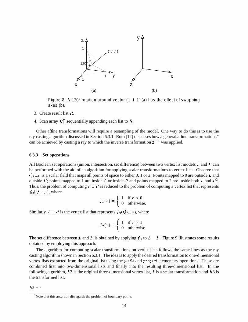
For example, a rotation of 120o around vector 1 � 1 � 1 can be thought of as swapping axes � with � , �with � and � with � (see Figure 8). In other words, a vertex at � � � � � would be moved to position � � � � � .The ordering scheme of vertex lists stipulates that the third coordinate ( � in the original list) is the primarysorting key, with ties broken by considering the second and first coordinates ( � and � , respectively). Noticethat the relative ordering of coordinates � and � is unchanged by the proposed rotation, i.e., if two verticeshave the same � coordinate values in the original list, then they will appear in the same relative order in therotated list. This means that a list for the rotated solid may be obtained by performing an order-preservingsort on coordinate � of the original list.

Assuming that the model was sampled in regular intervals along the � axis, say at � � 1 � 2 � ��� � , we coulduse the � coordinate values as an index. The idea is to distribute the vertices of the original list into anarray of “buckets” addressed by � , say

��� ��� . After all vertices were placed in some bucket, the contents of���1 � � ��� 2 � ��� � ��� � � are threaded together resulting in the reordered list. This is an instance of radix sorting.

To summarize:

1. Allocate an array of lists��� � , where each

��� � � will contain all vertices having � � � .2. Scan the original list appending each vertex at � � � � � to list

��� ��� .

13

x

y

z

120O

(1,1,1)1

11

x

y

z(a) (b)

Figure 8: A 120o rotation around vector 1 � 1 � 1 (a) has the effect of swappingaxes (b).

3. Create result list � .

4. Scan array��� � sequentially appending each list to � .

Other affine transformations will require a resampling of the model. One way to do this is to use theray casting algorithm discussed in Section 6.3.1. Roth [12] discusses how a general affine transformation �can be achieved by casting a ray to which the inverse transformation � � 1 was applied.

6.3.3 Set operations

All Boolean set operations (union, intersection, set difference) between two vertex list models � and � canbe performed with the aid of an algorithm for applying scalar transformations to vertex lists. Observe that��� � � is a scalar field that maps all points of space to either 0, 1 or 2. Points mapped to 0 are outside � andoutside � ; points mapped to 1 are inside � or inside � and points mapped to 2 are inside both � and � 2.Thus, the problem of computing ��� � is reduced to the problem of computing a vertex list that represents��� ��� � � , where

��� � ��

1 if � � 00 otherwise.

Similarly, ��� � is the vertex list that represents��� ��� � � , where

��� � ��

1 if � � 10 otherwise.

The set difference between � and � is obtained by applying���

to � ��� . Figure 9 illustrates some resultsobtained by employing this approach.

The algorithm for computing scalar transformations on vertex lists follows the same lines as the raycasting algorithm shown in Section 6.3.1. The idea is to apply the desired transformation to one-dimensionalvertex lists extracted from the original list using the ���� �� and � � ��� � � � elementary operations. These arecombined first into two-dimensional lists and finally into the resulting three-dimensional list. In thefollowing algorithm, � 3 is the original three-dimensional vertex list,

�is a scalar transformation and � 3 is

the transformed list.

3 ���

2Note that this assertion disregards the problem of boundary points

14

(a) (b) (c)

Figure 9: Set operations performed on vertex list models of a sphere and acubical block: (a) union, (b) intersection and (c) difference.

,2 ��� 2 � �

while�

3 ���� do� � last coord. of � ��#%'3� � 3 ��

2 � ���� �������� ���� ��(� � 3 ��� � ,2,

2 � �2�

3 �����"$#%��&(')��*� � 3 �2 �-�,1 ��� 1 ���

while�

2 ��-� do./� last coord. of ���#)' � � 2 ��

1 � ���� ����5��� ���� ��(� � 2 �7�(� ,1,

1 � �1�

2 �����"$#)� &(')��*� � 2 �1 � transform1D � � 1 0 ��2 ��#���� ��&('3� 2 054 &)���� ����5��� 1 6�� 1 0 .����� 1 �

1enddo

3 �-#���� ��&('3� 3 054 &)���� �������� 2 6�� 2 0 ���7�� 2 �

2enddoreturn R3

In the pseudo-code above, transform1D � 1 �� stands for a procedure that returns the one-dimensional

vertex list � 1 transformed by�

. This operation is trivial and will not be described here. The algorithmworks by disassembling � 3 into pieces of lower dimension using the inverse process employed in the raycasting algorithm. For instance, while in that algorithm the prefixes of � 3 were obtained by subtractingvalues of � 2 obtained in successive iterations of the outer loop, now it is necessary to add consecutiveprefixes of � 3 to obtain � 2. A similar process is used in the inner loop to obtain � 1 from consecutiveprefixes of � 2. Once � 1 is obtained, transform1D is invoked to compute � 1, its transformed version. Theassembly of � 2 from successive values of � 1 and of � 3 from successive values of � 2 follows the exactsame procedure used in the ray casting algorithm. Once again we need temporary variables � 1, � 1, � 2 and� 2 to hold previous values of � 1, � 1, � 2 and � 2, respectively, between iterations.

6.3.4 Displaying vertex list models

Modern workstations are equipped with high-performance graphic displays, often supported by hardwarethat permits very fast rendering of surfaces and lines in three dimensions. Therefore, in order to make

15

use of such capabilities, it is necessary to extract boundary geometric elements from the space occupancyinformation conveyed by vertex lists. Fortunately, vertex positions already provide the essential geometricclues. For instance, referring to Figure 7(c), we notice that the edges of the model have their endpoints atvertex positions.

A wireframe display of a vertex list model can be obtained by drawing edges parallel to the � , � and �axes. By traversing the list in its original order and drawing line segments between successive vertices weare guaranteed to draw all edges parallel to the � axis. However, some line segments will not correspond toedges of the model. It is clear that two successive vertices cannot form an edge parallel to the � axis if their �or � coordinate values differ. This can be worked around by applying the ���� �� / � � � � � � � � � operators twiceto break the list into several sublists all of which are guaranteed to contain vertices on the same � -parallelline (see Figure 10(a)). Examining one of these sublists we will notice that it represents a scalar field where

+1

+1

+1

-1

-1

-1

-1

-1

+2

xy

z

+1

+1

+1

-1

-1

-1

-1

-1

+2

+1

+1

+1

-1

-1

-1

-1

-1

(a) (b) (c)

Figure 10: Extracting edges along the � axis.

points are mapped to � 1, 0 or � 1, where edges will correspond only to the regions mapped to � 1 or � 1(Figure 10(b)). By using scalar transformation

���� (defined below) it is possible to obtain a list where theseregions are all mapped to � 1 (Figure 10(b)).

���� � ��

1 if ���� 00 otherwise.

The advantage of such a list is that it contains an even number of vertices and edges can be traced betweentwo consecutive vertices � and � � 1 only if � �� � � 1 and � � � 1 � � 1.

The pseudo-code below summarizes the algorithm to trace the edges parallel to the � -axis of a modelgiven by list � 3. Procedures edge endpoint 1 and edge endpoint 2 are primitives for specifying the twoendpoints of a line segment.

while�

3 ���� do� � last coord. of � ��#%'3� � 3 ��

2 � ���� �������� prefix � � 3 �7��3 �����"$#%��&(')��*� � 3 �

while�

2 ��-� do./� last coord. of ���#)' � � 2 ��

1 � ���� ����5��� prefix � � 2 ����2 �����"$#)� &(')��*� � 2 �1 � transform1D � � 1 0 ���� �

while

1 ���� do� � last coord. of � ��#)'3� 1 �� � weight of ���#)' � 1 �if � � ��� 1 then

16

edge endpoint 1 � � 0 . 0 �*�else

edge endpoint 2 � � 0 . 0 �*�endif

enddoenddo

enddo

In order to complete the drawing of the wireframe model it is necessary to trace the remaining edgeswhich are parallel to the � and � axes. This can be done by reordering the list as discussed in Section 6.3.2.This is done twice and each time reordered list is given as input the the algorithm above. Figure 12(a) wasproduced using this approach.

Two-dimensional boundary elements, i.e. faces, can be extracted from the model using a very similaralgorithm. In fact, we can modify the algorithm above to extract vertex lists that represent faces parallel tothe � - � plane as follows:

while�

3 ���� do� � last coord. of � ��#%'3� � 3 ��

2 � ���� �������� prefix � � 3 �7��3 �����"$#%��&(')��*� � 3 �2 � transform2D � � 2 0 � �� �

paint polygon � 2 0 �*�enddo

However, the task of drawing a polygon represented by two-dimensional lists (the intended meaning ofprocedure paint polygon above) is not trivial. The problem is due to the fact that common graphicrendering engines are only able to render simple polygons expressed as a list of connected edges, whereasthe two-dimensional vertex list may represent polygons with holes and/or delimited by disconnected contours(see Figure 11(a)). One solution would consist of converting the vertex list polygon into one or more

1 2

34

56

7

8 9

10

11 12

1314

1

2 34

5

6

(a) (b)

Figure 11: Complex polygon may be rendered by tracing the different contours(a), or by splitting it into a set of rectangles

polygons in the accepted format. This is doable, but unnecessarily messy. A cleaner solution is to split thepolygon into a set of rectangles by using a plane-sweep algorithm. In his pioneer work, Shechtman [18]shows how to split a polygon given in vertex list format into a set of maximal horizontal rectangles andproves that the total number of rectangles is never greater than the number of vertices of the input list (seeFigure 11(b)). Although simple enough, we will not reproduce his algorithm here.

Once a suitable implementation of procedure paint polygon is achieved, a complete rendering of themodel can be produced by applying the above algorithm three times, each followed by a rotation. Figure 12(c)

17

was produced with this approach. Hidden surface elimination was accomplished by depth-buffering. Asimple hidden-line rendering can also be achieved by first drawing all faces with depth-buffering enabledand then drawing the edges (Figure 12(b)).

(a) (b) (c)

Figure 12: Rendering of a simple mechanical part modeled with vertex lists.Wireframe (a), wireframe with hidden lines (b) and shaded (c).

7 Concluding Remarks

A new approach to modeling and operating on orthogonal objects in arbitrary dimensions known as a vertexrepresentation and implemented as a vertex list has been described. Although the basic idea has alreadybeen presented for two-dimensional data [18], our contribution has been the extension to higher dimensions.Its advantage lies in its compactness in comparison with more traditional representations such as rasters andcollections of hyperrectangles (disjoint and non-disjoint). Unlike arrays of voxels, the storage required forvertex lists is proportional to the boundary of the represented objects and remains invariant under scaling.Also, unlike CSG, normalized vertex representations have the property of being unique, a property that canbe exploited in many ways (e.g., Santos [17] showed how vertex lists are useful for the recognition of circuitelements in VLSI design).

Vertex lists are similar in spirit to chain codes with the advantage that they are not restricted to twodimensions. In particular, the elements of a vertex list can be ordered lexicographically. For example, 3Dobjects are ordered by faces perpendicular to the � axis. Algorithms have been given for generating vertexrepresentation models for primitive solids, performing affine transformations, set-theoretic operations, anddisplaying vertex representation models.

The vertex representation models the same objects that are obtained through use of methods such as anarray of voxels or octrees (i.e., objects with orthogonal faces). Its advantage is that it requires less spaceand unlike octrees its space requirements are not sensitive to translation. Moreover, it enables increasingthe quality of the approximation of objects by increasing the number of vertices that make up the model. Incontrast, increasing the quality of the approximation in a array of voxels requires doubling the resolutionwhich means a significant increase in the space requirements. A drawback of the vertex list implementationof a vertex representation is that it is not appropriate for localized querying — for instance, the extractionof the value of a particular point in space requires the traversal of the entire vertex list on the average.These operations can be performed better by imposing access structures such as point variants of quadtreesand octrees (e.g. [15]) on the vertex representation. Conversion of vertex lists to these other forms ofrepresentations can be done with little difficulty.

Another issue that springs to mind when considering the power of expression of the vertex representation

18

is whether it is possible to extend it to model non-orthogonal objects. In fact, we have preliminary resultsindicating that this goal is attainable by allowing vertices which represent different cone types. We expectto report these results in the near future.

8 Acknowledgments

We have benefited from discussions with J. Shechtman, whose work sparked our interest in vertex repre-sentations.

References

[1] B. G. Baumgart. A polyhedron representation for computer vision. In Proceedings of the NationalComputer Conference 44, pages 589–596, Anaheim, CA, May 1975.

[2] W. R. Franklin and V. Akman. Building an octree from a set of parallelepipeds. IEEE ComputerGraphics and Applications, 5(10):58–64, October 1985.

[3] H. Freeman. Computer processing of line-drawing images. ACM Computing Surveys, 6(1):57–97,March 1974.

[4] G. M. Hunter and K. Steiglitz. Operations on images using quad trees. IEEE Transactions on PatternAnalysis and Machine Intelligence, 1(2):145–153, April 1979.

[5] D. E. Knuth. The Art of Computer Programming vol. 3, Sorting and Searching. Addison-Wesley,Reading, MA, 1973.

[6] M. Mantyla. An Introduction to solid Modeling. Computer Science Press, Rockville, MD, 1987.

[7] D. Meagher. Geometric modeling using octree encoding. Computer Graphics and Image Processing,19(2):129–147, June 1982.

[8] D. Meagher. Octree generation, analysis and manipulation. Electrical and Systems EngineeringIPL-TR-027, Rensselaer Polytechnic Institute, Troy, NY, 1982.

[9] F. P. Preparata and M. I. Shamos. Computational Geometry: An Introduction. Springer–Verlag, NewYork, 1985.

[10] A. A. G. Requicha. Representations of rigid solids: theory, methods, and systems. ACM ComputingSurveys, 12(4):437–464, December 1980.

[11] A. A. G. Requicha and H. B. Voelcker. Solid modeling: a historical summary and contemporaryassessment. IEEE Computer Graphics and Applications, 2(2):9–24, March 1982.

[12] S. D. Roth. Ray casting for modeling solids. Computer Graphics and Image Processing, 18(2):109–144, February 1982.

[13] D. Rutovitz. Data structures for operations on digital images. In G. C. Cheng et al., editor, PictorialPattern Recognition, pages 105–133. Thompson Book Co., Washington, DC, 1968.

[14] H. Samet. Applications of Spatial Data Structures: Computer Graphics, Image Processing, and GIS.Addison-Wesley, Reading, MA, 1990.

[15] H. Samet. The Design and Analysis of Spatial Data Structures. Addison-Wesley, Reading, MA, 1990.

[16] H. Samet and M. Tamminen. Bintrees, CSG trees, and time. Computer Graphics, 19(3):121–130, July1985. (also Proceedings of the SIGGRAPH’85 Conference, San Francisco, July 1985).

19

[17] F. V. Santos. Extracao de circuitos VLSI. Master’s thesis, Eng. Eletrica, Universidade Federal do Riode Janeiro, Rio de Janeiro, April 1991.

[18] J. Shechtman. Processamento geometrico de mascaras VLSI. Master’s thesis, Eng. Eletrica, Univer-sidade Federal do Rio de Janeiro, Rio de Janeiro, April 1991.

20