FinancialInstitutionsCenter

Vertical Scope Revisited: TransactionCosts vs Capabilities & ProfitOpportunities in Mortgage Banking

byMichael G. JacobidesLorin M. Hitt

01-17

The Wharton Financial Institutions Center

The Wharton Financial Institutions Center provides a multi-disciplinary research approach tothe problems and opportunities facing the financial services industry in its search forcompetitive excellence. The Center's research focuses on the issues related to managing riskat the firm level as well as ways to improve productivity and performance.

The Center fosters the development of a community of faculty, visiting scholars and Ph.D.candidates whose research interests complement and support the mission of the Center. TheCenter works closely with industry executives and practitioners to ensure that its research isinformed by the operating realities and competitive demands facing industry participants asthey pursue competitive excellence.

Copies of the working papers summarized here are available from the Center. If you wouldlike to learn more about the Center or become a member of our research community, pleaselet us know of your interest.

Franklin Allen Richard J. HerringCo-Director Co-Director

The Working Paper Series is made possible by a generousgrant from the Alfred P. Sloan Foundation

2

VERTICAL SCOPE, REVISITED:

TRANSACTION COSTS VS CAPABILITIES & PROFIT OPPORTUNITIES IN MORTGAGE BANKING

Michael G. Jacobides

Assistant Professor of Strategic and International Management

London Business School

Sussex Place, Regent’s Park

London NW1 4SA, United Kingdom

Tel (011) 44 20 7706 6725; Fax (011) 44 20 7724 7875

mjacobides@london.edu

and

Senior Fellow, Financial Institutions Center

The Wharton School, University of Pennsylvania

Lorin M. Hitt

Alberto Vitale Term Assistant Professor of Operations and Information Management

and Senior Fellow, Financial Institutions Center

The Wharton School, University of Pennsylvania

1300 SH-DH, 3620 Locust Walk, Philadelphia PA 19104

lhitt@wharton.upenn.edu

3

VERTICAL SCOPE, REVISITED:

TRANSACTION COSTS VS CAPABILITIES & PROFIT OPPORTUNITIES IN MORTGAGE BANKING

Abstract

What determines vertical scope? Transactions cost economics (TCE) has been the dominant

paradigm for understanding “make” vs. “buy” choices. However, the traditional focus on

empirically validating or refuting TCE has taken attention away from other possible drivers of

scope, and it has rarely allowed us to understand the explanatory power of TCE versus other

competing theories. This paper, using a particularly rich panel dataset from the Mortgage Banking

industry, explores both the extent to which TCE predictions hold, and their ability to explain the

variance in scope, when compared to all other possible drivers of integration. Using some direct

measures of transaction costs, we observe that integration does mitigate risks; yet such risks and

transaction costs do not seem to drive firm-level decisions of integration in retail production of

loans. Rather, capability-driven and capacity- (or limit to growth-) driven considerations explain a

significant amount of variance in our sample, under a variety of specifications and tests. We thus

conclude that while TCE explanations of vertical scope are important, their impact is dwarfed by

capability differences and by the desire of firms to leverage their capabilities and productive

capacity by using the market.

Keywords: Mortgage Banking; Transaction Costs; Integration; Capabilities; CapacityConstraints; Limits to Growth

4

1. Introduction

What determines vertical scope? In the last three decades, transactions cost economics (TCE) has

been the dominant paradigm for understanding why firms choose to “make” rather than “buy”

required production inputs. The basic TCE argument is that the hazards of the market, especially

those created by information asymmetry, lead firms to increase vertical scope, while absence of

such hazards and efficiencies of production in specialized firms lead firms to use “the market”.

Several empirical studies on vertical scope have been produced over the last fifteen years, and in

most of them transaction costs (TC) have been shown to be of some import (see Shelanski and

Klein, 1995). However, the attention to validating or refuting the propositions of TCE and related

propositions from organizational economics may have taken the focus away from understanding

the different factors that can come into play in explaining vertical scope. Moreover, these studies

rarely explore the relative importance of transactions costs explanations as compared to other

possible theories.

Of late, a number of management scholars have voiced their concerns with the predominance of

TCE-based views of vertical scope, and there is a nascent “capability-based view” of integration,

which favors more the factors that relate to firms’ relative advantages, as well as other non-TCE

factors (e.g. Argyres, 1996). We consider this debate to be important, and believe that we are in a

dire need of direct empirical investigations not only of the validity of the TCE tenet, but also of its

relative explanatory power, especially when compared to other potential sources of explanation.

The setting in which we will analyze this empirical issue is mortgage banking – that is, the

segment of non-depository financial institutions which originate, process, approve, and then (in

most cases) sell mortgage loans to the secondary market. The mortgage banking industry is an

almost ideal setting to study vertical scope, as it has a complex value chain (see Figure 1) which

has increasingly been fragmented into quasi-independent parts, which are performed both by

integrated firms as well as narrowly targeted specialists. The feasibility of a wide range of vertical

scope decisions and the observed variety in the industry provide a rich setting for empirical study.

In addition, we have access to a previously untapped and highly detailed firm-level data source on

firm structure and productivity from the Mortgage Bankers Association, the leading trade

organization for the industry. This enables us to construct and validate measures for transactions

5

costs (a historically difficult empirical task) and vertical scope, as well as measures required to test

several other competing theories including the “capabilities-based” view, which we will also

analyze in depth.

-----------------------------------Insert Figure 1 about here

-----------------------------------

Our principal analyses will focus on the decision to integrate retail production (the process of

finding customers and closing the loans) along with other downstream activities (secondary

marketing or “warehousing”, and servicing1) for different types of loans. There are two potential

vertical configurations – firms can either use their own, captive retail branches to originate loans,

or they can use (partially- or fully-independent) outside brokers and correspondents. Through

these channels, firms can originate a variety of different types of loans (conventional vs. jumbo,

fixed vs. variable interest rate, government guaranteed) and can make different vertical scope

decisions for each type of loan. Because these loans vary significantly in their risk profile, degree

of potential information asymmetry, and capability requirements, we can examine how firms’

matching of channel to loan type is consistent or inconsistent with different theories of vertical

scope.

Using both industry-level and firm level data, we show that loan type is indeed a good surrogate

for transaction risks, and that vertical integration can help mitigate these risks, validating our

measurement approach. We then examine several different theories of vertical scope using an

unbalanced panel dataset of an average of 187 firms per year over ten years. We find that firms do

indeed have a greater degree of vertical integration for high-risk loans consistent with TCE, but

that TCE-related explanations account for only about 4% of the variance in our measure of

integration. Using two different measures of a firm’s capabilities (capabilities in upstream and

downstream divisions, respectively), we are able to explain up to 30% of the variance in

integration. These results appear robust to different specifications and analysis techniques

including robust regression and fixed-effects panel data models. Our results are not consistent

with simpler stories of vertical integration such as economies of scale or capital constraints, and

1 Secondary marketing or “wholesaling” is the management of the process between closing the loan for the retailcustomer and the resale in the secondary market. Servicing is the processing of ongoing transactional activity of a

6

given the nature of the industry do not believe that integration could be explained by non-

competitive effects (e.g., monopoly rent seeking and vertical foreclosure), the other leading

explanation of vertical scope. We thus conclude that while TCE explanations of vertical scope are

important, their impact is dwarfed by capability differences and by the desire of firms to leverage

their capabilities and productive capacity by using the market.

The structure of this paper is as follows: Section 2 reviews the relevant literature and theoretical

explanations as for the possible drivers of vertical scope, and we provide the hypotheses to be

tested. Section 3 explains our empirical setting, data and methods used. In Section 4, we examine

our measures of transaction cost, and how these are derived from existing theory. Section 5

provides contains the tests of both the TCE and the capability-based hypotheses, and compares

their explanatory power, giving due attention to control variables such as scale. Section 6

concludes by considering the theoretical and empirical implications of our findings.

2. Drivers of vertical Scope: Existing Literature

In the last thirty years, much discussion has taken place with regard to the role of transaction costs

in determining the decisions to use the open market rather than vertical integration. However, a

number of different factors can be put forth to explain vertical scope, both on the firm and on the

industry level of analysis.

In our setting, integration into retail production could be due to four reasons, according to the

extant literature. First, it could be the result of oligopolistic rent-seeking, as the industrial

organization literature suggests. Firms may want to integrate in order to “raise rivals’ costs”

(Salop and Scheffman, 1983), control scarce resources (Galbraith, 1967; Porter, 1980), eliminate

multiple marginalization2 (Salop, 1979; Dixit, 1983), improve the ability to price discriminate

(Wallace, 1937; Stigler, 1951; Arrow, 1975; Riordan and Sappington, 1987), or to obtain a

strategic upstream supply. However, in mortgage banking no firm has significant market power

overall or in the supply or consumption of any input or output in any segment of the value chain.

loan through the remainder of its lifecycle (e.g., collecting payments, generating statements and tax-relateddocumentation, and release of the lien at the end of the loan, among others).2 The essential argument is that when because monopolies distort prices and quantities away from the competitiveideal, a series of monopolies selling vertically to each other can create large inefficiencies because the distortions are

7

Therefore, it is highly unlikely that the exercise of market power is a significant factor in

determining vertical scope in this industry.

Second, integration could be due to scale, inasmuch as a minimum scale might be required to be

integrated, and hence vertical scope might be technologically determined. A closely related issue

is that size may be determined by capital requirements – integration may reduce overall volatility

and thus alleviate capital constraints for those without easy access to internal or external sources

of financing. Both of these explanations are testable, although our priors are that these are not

likely to be significant.

Third, it could be driven by the TCE-type costs of using the market. If the TCE hypothesis is

correct, then firms would decide their degree of integration on the basis of the transaction costs of

the loans to be procured. While asset specificity may not be particularly relevant in explaining

scope, transaction costs and information asymmetry may be a significant driver of vertical

integration. If there are loans whose attributes are unknown and hard to verify, and if some loans

have higher default risks than others, then firms should tend to produce these in-house, as market-

based procurement is bound to be fraught with transactional dangers (Akerlof, 1972; Barzel, 1982;

Williamson, 1985). That is, firms will be integrated in the production of loans that both have a

higher propensity to present problems, and where trading “through the market” exacerbates these

problems. In particular, the party that produces a loan may have an information advantage over

those that purchase loans, and may have an incentive to strategically withhold or misrepresent

information in order to close the loan and get the commission. Therefore, extant theory would

lead us to expect that loans with significant transactional hazards (the quality of the underlying

loan cannot be easily verified) should not be purchased through the market, but rather should be

“produced” in-house. Thus, integration should be a function of the loan type composition of the

origination portfolio: Firms trading in “dangerous” loans should be integrated, whereas “plain

vanilla” loans would be traded through the market.

The final possibility is that integration is largely a function of the capabilities of firms in particular

parts of the value chain, by their capacity constraints (and dynamically, their ability to grow each

part of the value chain) and by the existing opportunities to profit (Jacobides, 2000). That is, the

magnified at each step in the chain. Significant gains can often be had by coordinating production among successive

8

vertical scope of the firms under this hypothesis is to be explained by its abilities in each vertical

segment, and it may be the case that several firms may chose to specialize and use the market

despite the transactional risks that imperfect information on loans would impose (cf. Argyres,

1996, Langlois and Robertson, 1995). Simply stated, vertical specialization could be born from the

opportunities of gains to trade (Ricardo, 1844), despite the “taxes” that the market imposes

through transaction costs – much like international trade, which is driven by differences in

productive capabilities or by capacity (and which may or may not be curbed through international

taxation).

There are two basic drivers of such potential gains from trade. The first is a simple difference in

their capabilities: mortgage banks would use brokers or other firms to originate loans where their

in-house capability is inferior, even when added costs of transactional hazards are included. The

TCE framework already anticipates this story (see Riordan and Williamson, 1995; Williamson,

1999), although the production cost advantages are typically less emphasized than disadvantages

of transaction risks, and have not generally been directly incorporated in empirical analyses. As

Demsetz (1988), Winter (1988) and Langlois and Foss (1998) remarked, the TCE “school” seems

to focus excessively on the exchange conditions, disregarding the potentially much more

important production conditions and capability differences.

The second source of “gains from intermediate good trade” (and hence reason for using “the

market” rather than “the firm”) may be capacity constraints or limits to growth, an aspect of

capabilities that has not been explicitly considered in extant theory. Consider a bank that has

equally good origination and loan warehousing / secondary marketing, but has a higher capacity in

warehousing. Such a bank may decide to use the market for origination because its warehousing is

profitable even if it buys loans from the market, despite the fact that such purchased loans may be

more expensive to buy than to produce in-house, and regardless of the fact that there may be added

risks in using the market. This may also occur if say, origination is hard to scale in the short-run

(as it requires the physical outlay of branches, representatives, etc.) whereas warehousing may be

easy to scale up. This would predict downstream expansion concurrent with increased upstream

integration (see Jacobides, 2000, for formal proofs). A closely related, but distinct, story in the

dynamic setting is that limits to growth differ between segments. In our prior example, if it is not

monopolies – often this coordination is created by vertical integration.

9

time that prevents origination from being scaled, but simply that origination is subject to much

greater diseconomies of scale than warehousing, firms will expand warehousing and buy loans

from the market. Therefore, being profitable downstream should lead to a ceteris paribus greater

use of the market, which will be even more pronounced if (a) the upstream segment is not as

efficient; and (b) if the upstream segment is hard to grow. In our setting, we know that origination

is much harder to grow than secondary marketing (“warehousing”), hence we do expect to see

higher downstream capability to be associated with higher use of the market.

To summarize, vertical scope will be explained in terms of capabilities of the firms in the market;

if all firms have similar upstream and downstream capabilities, then no specialization will occur,

regardless of the level of transaction costs. On the other hand, if there is significant inter-firm

dispersion of upstream and downstream capabilities, then even in the presence of transaction costs

specialization will occur and intermediate markets will be active, motivated by the latent gains

from trade along the value chain. Differential limits to growth in each segment will exacerbate this

capability-driven integration. (A formal analysis of this “capability” and “limit to expansion”

hypothesis of vertical scope, with qualitative illustrations from the mortgage banking setting, is

provided in Jacobides, 2000).

Monopolistic rent maximization; scale; transaction costs; and capability differences/limits to

growth, then, are the potential explanations of vertical scope. Based on our prior discussion, we

know at the onset that all the neoclassical economic hypotheses as for why firms should integrate

can be ruled out. Thus, there still remain three different explanations: Scale; transaction costs and

risks; and capability differences. While the role of scale is not related to any particular hypothesis

(it is, quite simply, a significant issue we have to control for in order to have a greater degree of

confidence in our predictions), we still have two major theoretically-driven explanations for the

choice of scope on the behalf of firms.

First, TCE and institutional economics lead us to expect that (H1) Transaction Costs matter, and

that on the margin they drive firms’ choices of scope. In addition to this hypothesis, we also posit

that (H2) capability differences and limits to expansion drive vertical scope. Furthermore, the

more important empirical question is, if both H1 and H2 are supported, which of them is the more

successful in explaining variation in vertical scope. Thus, rather than simply examining the extent

10

to which the directional predictions do or do not hold, we will try to explore the extent to which

either of these two sets of complementary and compatible solutions explain the variance in our

setting.

3. Setting, Data, Methods

3.1. Setting: Mortgage Banking

Mortgage banks are the non-depository financial institutions that have grown from the

development of the securitized mortgage finance provision system in the US, illustrated in Figure

1. They originate loans, which they also service, but typically do not hold the loans as assets;

rather, they sell them to the secondary market through large securitizers (quasi-public such as

Fannie Mae and Freddie Mac or private such as Citibank Mortgage). Mortgage banks generated

more than 56% of the total loan production in 1999, about $660 billion in new loans. Mortgage

banks, therefore, are a very important sector, despite the dearth of studies thereupon.

-----------------------------------Insert Figure 2 about here

-----------------------------------

Mortgage banks make money in different parts of the value chain; a graphical representation in

Figure 2 summarizes the activities along the value chain. Profit is made in three increasingly

distinct areas: Loan origination; loan warehousing, wholesaling and secondary marketing; and

loan servicing. For the purposes of this paper, we will term the origination “upstream” (it’s the

“production” of the raw loan); and the warehousing and then servicing as “downstream” activities.

To understand how profits are made and how intermediate markets operate, it is easier to move

from the furthermost upstream segment – servicing, to the downstream activities. The mortgage

bank that has a loan to be serviced, earns money on (a) servicing fees, which are a percentage of

the balance outstanding- anywhere from 18 to 44 basis points, and (b) on escrows and other fees

paid by the borrower directly to the mortgage bank. Given the average costs in the industry, this

represents a comfortable spread that is earned, and hence servicing is a profitable business.

Therefore, a loan to be serviced represents an annuity.3 The fact that each loan has an annuity

value has led to the creation of “Mortgage Servicing Rights” (MSRs) which can also be sold to the

open market. Mortgage Banks can make money only in the servicing side of the business by

3 The specific value of this annuity is determined by the interest rate at which the loan has been made, the subsequentpossibility of it being refinanced, and the resulting expected life of the annuity.

11

buying MSRs and then servicing the loans for which they have purchased the portfolio, or only on

the production side by producing loans and then selling the MSRs, hence capitalizing the value of

servicing.

Moving further upstream, we go to the production side, where money can be made on two major

segments, as we can see from Figures 1 and 2. The first segment is loan origination, which is the

process of identifying and selecting borrowers, processing loan applications, and closing the loan

for the customer. Ability to reach and counsel potential borrowers, hand-hold them through the

process and help them close the loan is critical here. The second segment is loan secondary

marketing, which is also called loan warehousing, i.e. holding the loan which has been just closed

and until it is sold to investors to the secondary market (e.g. to Fannie Mae or Freddie Mac), and

then arranging for the transfer of the loan to the securitizer / secondary market investor. A

mortgage firm may also decide to sell the related servicing rights, or it will keep them for its

servicing portfolio. In this segment, money is made by effectively managing the pipeline of closed

loans and selling them to the investors at the best possible price; managing interest rate

differences, especially when loans are closed in rising interest rate environments, when they may

be refinanced before they even reach the ultimate investors; and packaging the loans for sale to

securitizers / secondary market investors.

This paper focuses on the decisions of scope with regard to the production of loans. We examine

what affects the decision of mortgage banks to remain integrated (producing the loans they sell

through their own captive branches or representatives) or become specialized in warehousing and

secondary marketing of loans which have already been produced by other firms’ branches or by

mortgage brokers (firms specialized solely in origination). Hence mortgage banks can chose their

vertical scope (and indeed can do so in real time, and on a per-loan basis) by deciding whether

they want to buy loans for warehousing “from the market”, or whether they want to produce these

loans themselves, through their own retail network. So mortgage banks can be active downstream

(warehousing, servicing), upstream (retail production) or both.

What makes this setting particularly interesting is that we have loans that differ markedly with

regard to their transactional attributes, as well as to their risk profiles – and the downstream side of

12

the business (warehousing) can be affected by information misrepresentation of the upstream side

(production). Hence we might expect that firms would be reluctant to buy “dangerous” loans,

which are characterized by high transaction costs, but would gladly buy the “plain vanilla” ones.

This would mean that transactions costs would really affect the extent of integration.

Alternatively, it may be that the capability of each firm on each segment is the primary driver of

scope.

3.2 Data: The MBFRF

The data we have on mortgage banks comes from the quasi-regulatory Mortgage Bankers’

Financial Reporting Form (MBFRF) that they submit to the Mortgage Bankers Association.

These statements describe in very fine detail their operations, margins, per segment activities, loan

portfolio, pipeline composition, and a variety of other operational or financial characteristics. The

data covers around 36% of total mortgage loan volume originated in the U.S and contains an

average of 187 firms over 10 years (although it does not track the same firms each year). As this

data is collected for quasi-regulatory reasons, MBA tries to capture all the types of firms in its

survey, thus leading to healthy levels of variation. Given that the MBFRF is used to compile key

industry statistics, and that it is the only data that investors have for mortgage bankers, substantial

time and attention is expended on preparing it. It should be noted that this is the first time that any

strategy research is done on this data; moverover, this data has never been made available for

analyses of any type on the firm level of detail. The reason for MBA’s reluctance to let researchers

use the data has to do with the wealth of firm-level detail, which were able to get through a

carefully structured data analysis mechanism that preserved bank anonymity while allowing us to

test firm-level hypotheses.4

The MBFRF contains information on a number of different items. First, in contains information on

the composition of the origination portfolio of each firm, by loan type. Second, it contains detailed

information on the default rates of the firms’ loans closed. Third, it contains information on all the

balance sheet and income statement lines that are relevant in this industry. More important,

4 Note, however, that although we were allowed to run regressions on the full data and obtained all the results andstatistics for our analyses, we did not have the possibility to examine each observation separately, so as to ensure theconfidentiality of the data. This is one of the reasons for which we use extensively the robust regression technique,which we will explain shortly, that successfully deals with outliers, as we could not examine each specific outlier case.

13

perhaps, it contains income level information per stage of the production process (that is,

separately for retail production and wholesale production, as well as servicing). From this

segment-level income statement, we created performance metrics (margins or income per loan)

that gauge the efficiency of mortgage banks in each type of activity. Such metrics are often used

by practitioners to measure the health of a mortgage operation. The major dependent variable we

will want to explain is RPOALNPD, which is the percentage use of retail over total production.

RPOALNPD thus measures integration into the retail production. Other dependent variables are

used as well; all variables, dependent and independent, are listed in Table 1, which provides their

description and symbols.

-----------------------------------Insert Table 1 about here

-----------------------------------

Note that in addition to the MBFRF data, we also use the aggregate data on characteristics of all

mortgage loans (volume, type, default risk, etc.), as collected by the Department of Housing and

Urban Development (HUD) and reported through Inside Mortgage Finance publications. This data

is used to provide yet another check on the “riskiness” of different loan types.

3.3. Methods

There are three different types of tests we use in our empirical analysis. First, for examining the

relative risk of the various loan types, we use the non-parametric sign-rank tests (the Mann-

Whitney two sample statistic), which establish whether the means of two populations are identical

– an established method, discussed in Wilcoxon (1945), and Mann and Whitney (1989). The

second family of techniques, which is the most extensively used in this paper, consists of different

variants of regression analysis. For most analyses we report the results from ordinary least squares

(OLS) with all firms and years pooled, and parallel robust regression estimates that iteratively

reweights points that have a high influence on the coefficients as measured by Cook’s distance to

reduce the effect of outliers (Cook, 1979; Berk, 1990; Hamilton, 1991).5 Given that in a

financial industry we tend to have significant problems due to outliers (financial assets and returns

vary much more widely than in “real” corporations), and as we cannot do a case-by-case analysis

5 This procedure estimates an OLS regression, calculates the Cook’s D influence statistic and then reweightsobservations based on this statistic for a generalized least squares (GLS) regression. We utilized the rreg procedurein Stata using the default parameters.

14

of the outliers due to the confidentiality agreement, this technique is particularly helpful,

especially in the correlation between non-scaled measures (e.g., assets).

Given that we have panel data, we can also perform fixed-effects regressions (see e.g., Baltagi,

1995), which effectively control for time-invariant firm specific factors. We typically use these

analyses for two purposes: 1) investigating the robustness of our general results, and 2) examining

the effect of changes in various factors rather than levels, which are measured in the OLS/robust

regressions.

Finally, we do our comparisons of the predictive ability of various theories by comparing the R2

figures for each regression (or alternatively, the regression F-statistic) and by using scatterplots

which, as we will show later, provide a clear contrast in predictive ability that is not reliant on any

particular set of statistical assumptions.

4. Assessing Transaction Costs: Loan Type and the Role of Lemons

While we do not have any direct measures of transaction costs, we do have information about the

different types of loans. The perception in the industry is that loan types differ with regards to

information mis-representation, transactional problems, and the possibility of default. With default

come significant costs not only to the secondary investor, but the mortgage banker as well.6 In

this subsection perform two types of tests to validate that variation in transactions cost are indeed

captured by variation in loan types. First, we show that different loans vary systematically in their

risk of default – when there is larger quality variation in the underlying loan pool, it exacerbates

problems of information asymmetry and opportunism as the information needed to manage these

risks may be imperfectly communicated across firm boundaries both unintentionally and

strategically. Second, we show that vertical integration can reduce default risk, suggesting that

integration is indeed a policy instrument that enables this risk to be managed as would be

predicted by TCE.

6 Loan defaults are costly for mortgage banks in several ways. First, if a loan defaults and there were underwritingerrors, mortgage banks are often obligated to buy back the loan from secondary investors and bear the credit lossdirectly. Secondly, even if the mortgage bank is not responsible for credit risk (for example, due to a Government

15

In Figures 3a and 3b, we plot Department of Housing and Urban Development data over the

period 1989-1999 on (a) total delinquent loans (i.e. loans in arrears greater than 30 days, bad

loans, etc), and (b) of loans foreclosed, where the property has been taken from the proprietor.

The data are aggregated to three major loan categories: FHA (Federal Housing Authority) loans,

VA (Veteran Administration) loans (a.k.a. Government loans) and conventional loans, where

FRM’s (Fixed Rate conventional Mortgages) and ARMs (Adjustable Rate conventional

Mortgages) have been bundled together. The figures clearly show a significant difference in credit

risk between the various loan categories. With these yearly averages, the non-parametric

Wilcoxon sign test that the mean delinquency and default rates are the same for government loans

and conventional loans is rejected (p<.00001). If the two loan types were the same, we would

expect that conventional loans would have a higher default rate than either government loan

category in 5 out of 10 years, in our sample, it is 0 out of 10 for both types. Within the

conventional loan category, we have further data on the differences between ARMs and FRMs

produced by Freddie Mac. In these loans, we see that ARM’s are indeed more prone to default

than the FRM’s (Wilcoxon sign test, p<.00001).

-------------------------------------------Insert Figures 3a and 3b about here-------------------------------------------

Our results suggest that defaults are higher in the government categories- FHA/VA; then come

ARM’s; and then FRM’s. Qualitative evidence supports and explains this tendency. The reason for

higher defaults in Government loans, for instance, is that the minimum requirements on these

loans are more “generous”, as a matter of social policy. This means both that the mean default is

higher (adverse selection is encouraged in FHA/VA loans) and that there should be a higher

variation around the expected returns mean. Similarly, ARMs have significantly higher risk

because they are utilized by customers with less financial strength (due to lower initial interest

rates) which is exacerbated by the presence of varying monthly payments, especially when interest

rates are volatile or rising. In such cases, marginal borrowers can produce greater foreclosure and

delinquency costs. So, aggregate data suggests that transactions costs are highest in Government

guarantee), managing default creates significant operational costs of collections, foreclosure and subsequent assetmanagement. Thus, the costs of procuring a “lemon” from the market is large.

16

loans, somewhat lower in ARM conventional loans, and lowest of all in the plain vanilla FRM

conventional loans.

These differences in loan risk are mirrored in our more detailed, firm-level data from the MBFRF,

also over the period 1989-1999. We consider the same categories as before, but can also include

larger “Jumbo” loans from 1996-1998.7 This is important as it also establishes the trends within

our own data, and enables us to investigate whether higher mean default rates are also associated

with higher variance in default rates across firms. Greater heterogeneity of borrowers may also

lead to greater variance of defaults across firms if firms have different capabilities in managing

credit risk (either due to their ability internally, or their ability to manage external contractors).

-----------------------------------Insert Table 2 about here

-----------------------------------

These arguments are borne out in our data (see Table 2) – government loans are indeed more risky

than conventional loans in both mean and variance terms. FHA-VA loans have higher default

rates in 892 observations (firm-year) compared with only 204 firm-years of data where

conventional has a higher default rate (Mann-Whitney test of equality rejected, p<.0001). The

evidence is less clear for the difference between FRMs and ARMs – ARMs are higher risk in

52.1% of the observations, which enables us to reject equality with the Mann-Whitney test only at

p<.08. Jumbo mortgages are in the middle, a higher mean than conventional and a much higher

variance (the point estimate of the variance even exceeds that of Government loans). This

suggests that Jumbos are somewhat riskier in general and may also require specialized skills,

given this higher variance in outcomes.

Collectively, these tests indicate that there are systematic differences between each loan type, and

that it would be reasonable to expect these differences to affect the expected transaction costs and

dangers for each category.8 But, the question becomes, just how reasonable? It may be that each

loan type differs by the extent to which it creates a risk (in terms of expected loss), but perhaps in

this industry, trading loans through the market has no real “transaction cost”; perhaps integration

7 Jumbo loans are those with initial outstandings greater than ~220K. This is approximate, as the cutoff has increasedover our sample period.

17

into retail does not mitigate risks, and thus the fact that some loans are riskier than others would be

inconsequential with regard to the choice of vertical channel. To resolve this important question,

we have to look at the extent to which in-house procurement is negatively associated with default.

If making rather than buying loans lessens the risks for these loans, then there are some true

transaction costs of using the market. And hence our suggestion that higher-risk loans ought to be

made in-house rather than purchased would be a faithful and consistent application of TCE.

-----------------------------------Insert Table 3a about here

-----------------------------------

In Table 3a, we report robust regression results that relate firm level risk of default to integration

for each category of loan (different columns of the Tables). We begin first with an integration

measure of retail production (fractions of loans produced in each category). Starting with the

“high-risk” loans (FHA-VA), we see that the expected negative correlation between the degree of

integration into retail production and the level of defaults does obtain, and with a statistically

significant margin. The more retail is used, the smaller the default rates. If we look at the second

most “dangerous” category, ARM’s, we see that the same patterns still obtain. The same happens

with the third “risky” category, Jumbo loans. Interestingly, the impact of the choice of a

procurement channel is statistically stronger here, although its coefficient is roughly equal to that

of the ARM. This finding is in line both with our theoretical expectations, and qualitative

evidence. Jumbo loans not only have a relatively higher default rate, but also the highest variance,

and therefore it is to be expected that producing these loans in-house is particularly helpful in

mitigating loan defaults. In the “plain vanilla” FRM category, on the other hand, production mode

does not seem to be particularly important, as the coefficient is essentially zero. This is probably

because the informational discrepancies between in-house and market-based origination are so

limited that it does not make much difference how the loan is produced, consistent with a more

elaborate TCE explanation. Interestingly, these results are similar in magnitude and statistical

significance (except for the ARM result) if we lag the dependent variable by one or two periods

which allows for some adjustment in outcome since default outcome typically follows origination

(one period lags are shown in Table 3b, two period lags not shown).

8 These results also hold in aggregate – the larger the fraction of high risk loans in a firms’ portfolio, the greater risk ofdefault overall (results not shown).

18

-----------------------------------Insert Table 3b about here

-----------------------------------

These regressions suggest that the use of the market is indeed associated with higher risks, and

that, especially for the riskier types of loans, it is indeed beneficial to avoid brokers and

correspondents – just as TCE would suggest. Further evidence that using the market matters to the

eventual risks, and that each loan type differs both for the risks and for the extent to which the

market is desirable, can be obtained by the regression of per-category defaults on whether the

loans were produced (warehoused) by the firm that services them, or whether they were bought on

the open market – that is, whether there was full vertical specialization. To do that, we regress the

default percentage to the extent to which loans were purchased as closed loans or as Mortgage

Servicing Rights. As this is a measure of specialization rather than integration, TCE would predict

a positive correlation.

-----------------------------------Insert Table 4 about here

-----------------------------------

The results reported in Table 4, again by loan category. The independent variable is the extent to

which loans serviced were purchased from the open market (servicing released or as MSR’s); the

specific regressor is lagged for one period (similar results hold for either two or zero lags, not

shown). These results indicate that “full marketization” comes with significant dangers. The more

the market is used, the greater the possibility of default, in each loan category. Hence if the market

is relied upon to obtain everything but the servicing rights, even the plain vanilla loans may

exhibit transactional problems. Also, the impact of using the market differs between loan

categories, as we also observed in the previous set of results. The coefficient of FRM’s is around

.002; for the more dangerous ARM’s and Jumbos it is around 0.004; and for the most dangerous

FHA/VA around 0.08. Hence the more risky / uncertain the loan, the greater the benefit from

producing it in-house, in terms of risk mitigation.

In conclusion, we do have evidence that (a) loan types are a good proxy for transaction costs; (b)

production choices (degree of integration) do mitigate these risks, especially in the most dubious

products. Therefore, our data enables us to bypass one of the major problems in measuring the

19

drivers of vertical scope – namely, the difficulty of finding adequate measures of transaction costs.

This allows us to provide unusually direct tests of the theory, to which we move.

5. Explaining Vertical Scope: Transaction Cost, Scale, and Capabilities

In the following sections, we systematically evaluate different possible explanations for the

integration decision.

5.1. Vertical Integration and Transaction Costs

In the previous section, we saw that the TCE rationale (that integration helps mitigate risks) is

correct. We also saw that loan types come with different transaction costs, and that integration

protects firms from hazards, especially in the high-risk loans. We thus concluded that we can use

loan types as a reasonable surrogate of TC, and that we would expect that origination portfolio

composition should be a statistically significant driver of integration. But the question now

becomes, how important is it, really?

The first objective is to examine whether the degree of integration in origination is determined

types of loans that a firm produces. The general model we will estimate relates percentage of

retail loan production (overall) to the composition of loan production in different types and

various control variables. In all specifications we will include time dummy variables to capture

short-term effects of loan composition and also to partially correct for the mean integration

changing over time due to changes in the sample composition in our unbalanced panel. TCE

would predict a significant positive correlation with the number of government (FHA / VA) loans,

and a mild negative with FRM’s, the plain vanilla safe haven. Also, as most of the variation in

integration choices should be due to transactional factors, we would expect a significant degree of

variance explained by this regression. The results of this analysis are shown in Table 5, where we

estimate this base model with OLS and robust regression, and on the full sample versus a

restricted sample where we also have Jumbo loan production information.

-----------------------------------Insert Table 5 about here

-----------------------------------

A number interesting results stand out from these regressions. First, the total percentage of

variance explained is very small; the R2 is around 2%. If the year dummy variables are removed,

20

this is even lower without a substantial change in the rest of the results. Second, the statistically

significant coefficients are not quite in the direction that we would expect on the basis of our TCE

predictions. In the OLS regressions, we do observe a negative association between FRM and

degree of integration. This finding, however, becomes statistically insignificant when we move to

the more reliable robust regressions. As the FRM’s are the least risky loans, it would be

reasonable to expect to see a smaller degree of integration in the presence of a high proportion of

FRM’s. On the other hand, given that the previous sets of regressions indicated that the choice of

loan channel does not help mitigate transaction risks for FRM’s, we are cautious about this result.

The more interesting finding, however, is that the most “dangerous” category (FHA / VA) isn’t, as

expected, positively associated with integration, either in the entire sample, or in the post-1996

sample, which includes Jumbos. Furthermore, the coefficient of the FHA loans, in the more

reliable robust regressions, is a higher negative number than that of the “docile” FRM. That is,

having more FHA-VA’s than FRM’s seems to be positively associated to specialization, contrary

to what we would expect on the basis of TCE.9

Another interesting result is the strong negative coefficient on Jumbo loans (columns 2 and 4),

which means that the more Jumbos a firm has, the less it tends to use its own retail network. This

was not expected, due to the fact that (a) Jumbo loans have high risks, and (b) retail production has

the highest impact on Jumbo loans – this is the category where default is mitigated the most when

loans are produced in-house. So this result runs against the grain of the TCE predictions.

As a final test, we perform the same regressions described earlier in a fixed effects model,

essentially including a separate dummy variable for each firm to remove any firm-related effects

that are constant over time, and thus focus on changes on the margin. There are a variety of

reasons (some more plausible than others) why it might be useful to remove firm effects from the

analysis. It may be that each firm faces a different transactional environment (while this is highly

unlikely in our context, and our qualitative evidence points away from that, we still concede this

possibility). Perhaps some other factors shape the absolute level at which the firm can be

integrated – for example, age or local access to correspondents or brokers. Thus, a refined TCE

9 The qualitative assessment of this result from industry experts has been that retail branches are usually better able toseek and aggressively serve that particular part of the market- a capability hypothesis that we cannot test. Yet it is

21

argument would suggest, even if each firm’s level of integration may be due to such firm-specific

factors, the decisions of the firm on the margin should be affected by the expected impacts of

transaction risks, driven by the underlying loan attributes. Thus, if a firm increases its share of

FHA/VA, it should be expected to increase its degree of integration, for whatever level of

integration it is in. To see if this is the case, we ran the fixed-effects panel model on the data, with

and without the Jumbo loans.

These results (Table 5, columns 5 and 6) are remarkable. First, the explanatory power (once the

firm effects are removed) is practically nil. Firms, even on the margin, do not base their

integration decisions on the loan types and the resulting levels of expected transaction costs. There

is quite simply another set of factors at play. Second, even the limited statistical evidence in this

analysis runs against our theoretical predictions. The coefficient for the FHA/VA loans is

negative; that is, a firm which increases its share of more dangerous loans, where integration

would help it keep the risks down, appears to move concurrently to greater outsourcing.

To conclude, the evidence is that loan types do not drive the degree of integration, although they

do mitigate transaction risks. The explanatory power of transactional variables (or their proxies)

appears to be low, and the results often run against the grain of our theoretical expectations. Thus,

while we do find support for some aspects of TCE (regarding risk mitigation), it is not particularly

good at explaining heterogeneity across firms. If integrating mitigates the risks, then why should

integration not be associated with the reliance of potentially costly loans? The answer seems to be

that there are other factors at play – which is the impression we obtained from the qualitative

analysis and by archival research. The question now becomes, what are these other factors?

5.2 Firm-Specific Drivers of Vertical Scope

In order to see whether there is some firm-specific driver of vertical scope, which cuts across loan

categories, we examine how the percentage use of retail in one category (FRM conventional loans

– the biggest category) is associated with the percentage use of retail in the other production

categories. The basic premise is that we do not have any a priori expectation that the integration is

clear that the TCE hypothesis cannot find support.

22

one loan type will co-vary with that of another. As a matter of fact, we would expect the

association between different loans to be negative inasmuch as these would represent different

transaction costs; integration in high-TC loans like FHA-VA should be negatively associated with

low-TC loans like FRM.

Rather than doing a simple correlational analysis, we will provide a regression. This is

mathematically equivalent, but it also enables us to use the more reliable robust techniques. We

regress the integration of FRM loans on the integration of all the other loan categories to see

whether we will obtain this conditional relationship (negative or zero) as hypothesized by TCE, or

a positive relationship which cuts across loan categories, presumably driven by some firm-specific

capability or resource constraints. We include year dummy variables in all specifications. In this

analysis, we care about the sign of the coefficient and the degree of variance explained; the

specific point estimates obtained are not to be interpreted (as the choice of which variable is

dependent and which is independent is arbitrary). The analyses were done both in OLS and in

robust regressions, and were run separately in the full sample and the restricted sample which

includes Jumbo loan information, as before (Table 6).

-----------------------------------Insert Table 6 about here

-----------------------------------

The results are stark. In the simple model (OLS) between 71% and 82% of the variance is

explained (as opposed to 2-3.5% in the TCE-based model presented in the previous section). The

explanatory power is even stronger in the robust regressions, although the coefficients are not

particularly stable – this is likely due to substantial multicollinearity between integration in

different loan types (this multicollinearity is to be expected if our predictions on firm-specific

factors are correct). All loan types are very strongly and positively associated with the mode of

production of FRM’s, with t-scores from the teens to close to three hundred. If a firm tends to use

retail to procure only a portion of its FRM loans, chances are it will do the same with its

Government (FHA/VA) loans, despite the drastically higher TC in FHA/VA. As before, the year

dummies do have some explanatory power, but they account for only a small fraction of the

variance explained (~1-2%). Thus, there is something which is firm and year specific in the

decision to integrate, and which explains almost all the variance; and this is apparently unrelated

to TC.

23

Overall, our analysis suggests that firms do not chose their degree of integration on the basis of the

transactional properties of the underlying loans, despite the fact that (a) such loans have a

significant difference in their potential risks / costs, and (b) that the choice of procurement mode

mitigates these risks. We also see that the degree of integration co-varies very strongly within

firms across loan types. To further explore this finding, we estimate fixed effects regressions to

understand whether it is due to static firm-specific factors or whether the relationship is also

dynamic (that is, each firm could have a resource / expansion constraint that makes it change its

scope, for all loan types, in the same way each year, over and beyond its mean level.) The

capability – limits to growth model would lead us to expect both, which should appear as positive

correlations between integration in different loan types with and without fixed effects. Note that a

TCE story in this model would again posit negative relationships between integration in the

different loan types – firms choosing to outsource some loans will do this in the lower TC

channels, while integrating loans in the high TC channels.

We show the results of fixed effects models in Table 6, columns 5 and 6. In both of these models,

the correlations are large and significant. While the significance of the coefficients falls

noticeably, going from t-value close to 300 to t-values of 11 and less, the same general patterns of

a positive association between loan types with a firm remain important, even in the fixed-effect

context. The coefficient values are, as we expected, generally reduced – the joint impact of the

integration of all the other loan types added together is reduced from .99 or so to around .7. A

subtler change is that the extremely strong association of ARM’s with FRM’s is reduced when we

introduce the firm fixed effect. So, in the presence of a firm-effect, we see a more “balanced”

pattern whereby FRM’s co-vary “equally” with all loan types.

One striking observation is that dynamic (non-firm effect) factors appear to account for a very

large faction of the variance – if capabilities were constant over time we should see virtually no

correlation between retail integration in a fixed effects models. There are two possible

explanations for this finding. First, we could take the result at face value and conclude that which

implies that most of the “action” is dynamic – it is the firms’ adjustments to resource constraints

24

and expansion opportunities (the limits to growth hypothesis) that explains the match between

integration of different loan types.

However, it may also be due to a closely related story of modeling error. The fixed effects

regression will remove all the variance if indeed the structure of the firms over time are roughly

constant. A sub-study for M&A’s which we did with the MBA, revealed 101 Mergers or

Acquisitions in our sample. Given that the firms for which we have more than 2 periods are 369 to

459 (depending on the variables required for the analysis), this amount of M&A is enough to

contaminate the importance of the firm effect. The reason is that what is a firm with a set of

capabilities C1, leading to a choice of integration I1 at some initial time, will become a different

firm, with a different set of capabilities C2 (and resulting integration I2) after a merger. We also

have a reason to suspect that the difference will not be randomly distributed since M&A is one

common way for financial firms to acquire new capabilities or overcome barriers to expansion

(e.g. a servicing mostly mega-firm gobbles up an origination firm to ensure smooth flow of

servicing in the future) -- this further decreases the magnitude of the firm-effect. The fixed-effects

coefficient cannot “find” the commonalities of firms across different time periods because the

firms are indeed different. And given that 24-31% of our sample has undergone such activities, we

have good reasons to believe that, with our current data, the impact of the firm effect is

systematically under-estimated, and, unfortunately, the obvious solution of identifying M&A in

the sample is not feasible due to our data privacy restrictions.

5.3. Vertical Scope and Firm Scale

It appears that the capability and growth dynamics we suggested are consistent with the data, that

transaction costs are not the primary driver of vertical scope in our sample, and firm- and time-

specific factors can explain the choice of vertical scope. This being said, it would be clearly

premature to jump to a conclusion that this finding lends support to a capability-based approach.

What we first have to establish is that there is no other, obvious candidate that explains this

important firm-specific component – such as economies of scale.

25

In order to test whether scale affects integration, e.g. by requiring some minimum amount of loans

before in-house production becomes economically feasible, we estimated models that relate firm

assets and firm capitalization (equity) to the overall degree of integration. If there is some

minimum scale or if scale is a requirement for integration, then we would expect either a

monotonically increasing relationship, either approximately linear or on the increasing portion of

an inverted-u relationship. A similar relationship could also hold for financial capital if there

exists some minimum scale for capital; an opposite relationship could hold if integration smoothes

volatility and therefore requires a firm to have less financial capital. Different variants of this

analysis are presented in Table 7.

-----------------------------------Insert Table 7 about here

-----------------------------------

Note that rather than a normal positive association between asset size and degree of integration, or

even an inverted-u shape, there seems to be a u-shaped relationship (a negative coefficient on the

linear term and a positive coefficient on a quadratic term): small firms are integrated, then grow

and then become dis-integrated further on at very large scale levels. So scale is not a real driver of

vertical scope. (It is hard to justify a “u” relationship between size and integration on the grounds

of economies of scale). Qualitative data are consistent with this observation. Very small firms,

according to additional MBA surveys, are integrated, relatively larger ones make greater use of

their warehousing network (being less integrated), and some of the larger ones may be in between,

using both their retail network and brokers and correspondents.

The reason for which the asset-squared coefficient is positive, i.e. that there is some increase of

integration as firm size increases, is that the very big firms (which are more than two orders of

magnitude bigger than the average firm) are usually less integrated than the medium-sized firms.

The statistical reason we observe this is that the extrapolation of a linear trend would make us

expect that larger firms would not have any retail production (whereas in reality they have 30-60%

of their production in retail.) The business reason for which some of the larger players use their

in-house staff more is that they tend to be the mortgage banks that are large enough to engage in

national advertising, like Norwest / Wells Fargo, CitiMortgage or Countrywide. Smaller players

are more integrated as their comparative advantage lies in origination, hence they would not be

interested in purchasing others’ loans.

26

The same logic applies to equity as well. The relationship between integration and equity is also

negative – meaning that the more firms become capitalized, the less integrated they become, with

capital being measured in absolute terms.10 Similar results were obtained through both a log-level

and a log-log regression. The coefficients on log(assets) for the log-log regression are negative,

meaning that on average an increase of scale leads to a decrease of integration. To provide yet

another test, we examined whether an increase of a particular firm’s size or equity level was

related to an increase to its degree of integration. The fixed-effects models presented in the last

two columns of Table 7 suggest that firms that as firms grow, they tend to shrink their retail

network. This is squarely inconsistent with an economies of scale hypothesis.

We should, however, note that the fixed-effect model also indicates that the growth in equity size

(up to a limit, as the squared term is negative) is associated with an increase in integration; the

same result obtains for capitalization (equity/assets). So it may be the case that integration into

retail is associated with added requirements for capitalization. However, the regression results and

visual inspection of the data suggest that there is no evidence of a “limit” preventing small firms

from becoming integrated. There may even be a case for dis-economies of scale, or at least of

growth for retail; as a firm increases in size, this regression tells us, it is more likely to become

more vertically specialized (albeit with some limit as firms grow.). While this finding is too

isolated to provide adequate support for our “impediment to growth” hypothesis, it clearly points

away from the “usual suspects” such as scale and capital as drivers of scope.

5.4. Firm-based Proclivities: Capabilities (Efficiency Measures) and Integration

The results from our analysis strongly suggest that there are some firm-specific factors which

affect the degree of integration; these effects are not driven primarily by scale, and they also tend

to exist both on the cross-sectional level (each firm having a different proclivity to use retail,

across loan categories) and, more so, at the dynamic level (each firm deciding, year-per-year, how

to shift its entire production strategy, irrespective of loan type and the resulting TC levels). The

10 The capital structure, expressed here as equity over total assets is positively associated with the use of retail; soproportionately well capitalized firms may tend to use retail more; yet this does not relate to size. Equity levels,however, do.

27

question now is, what is this firm-specific factor? The answer that some recent research provides

is, “mostly, capabilities” (Argyres, 1996), as well as “limits to adjustment” (Jacobides, 2000).

Unfortunately, these constructs are not directly measurable. However, we can provide some

indirect evidence based on productivity measures, to the extent that capabilities should appear as

higher (relative) efficiency.

The best measures that we can use are the productivity metrics we have on the level of the

production employees per loan. Specifically, we will use the measure of the number of Full-Time-

Employee equivalent in retail production and divide it with the number of loans produced; and

likewise, we will take the number of FTE’s in origination overall (including Warehousing /

Wholesaling / Secondary marketing) and divide it with the number of loans produced (total).

The problem in estimating this relationship is that we have two opposing effects. On the one hand,

the more a firm is integrated into retail, the more employees that firm will have. By using the

market, a firm trades off salaried labor (FTE’s) to work done on a contract. So we expect for this

simple reason to see the degree of integration be positively associated with the number of

employees per loan handled. On the other hand, though, the better a firm is in the production stage

itself, that is, the fewer people it needs to originate a loan, the more it will be integrated – if it is

efficient at it, it will probably chose to do more of it itself.

To separate out these effects, we can obtain simultaneous estimates of three different productivity

measures we have available The first measure, FTEorpv, is the overall number of employees for

each loan, for the entire origination process (divided by the number of all loans, originated by all

channels). The second measure (FTEprpv) is the number of FTE in retail production – divided by

the number of loans produced only. The third measure (FTEwmpv) is the number of FTE’s used in

warehousing and purchased production, divided by the loans of that category.

The expectation is that the positive association between the extent of retail and the degree of

integration would be captured by the overall efficiency / staffing figures – that is, the more

integrated the firm, the higher the overall number of FTE per loan. On the other hand, the local

efficiency in production should lead to greater integration – firms that are good at retail, will do

28

more. (Hence the more FTE’s are needed for a loan, the smaller the degree of integration into

retail). Finally, if a firm is particularly adept in the warehousing side, i.e. if it has a low FTE, then

we would expect it to leverage this by using the market, ceteris paribus. So we would expect a

positive association between the number of employees (inefficiency) in warehousing and the

degree of integration. The results of the correlations, in OLS and robust regression are provided in

Table 8.

-----------------------------------Insert Table 8 about here

-----------------------------------

As shown in the table, the hypotheses on both upstream and downstream capabilities are borne

out. Also, despite the relative lack of sophistication in our measures, the variance explained is

above 30%, even in OLS regression (again, compared to the 2-4% of the TCE-based analyses). It

appears that inasmuch as firms are efficient in retail production, they tend to focus on it, and be

integrated in it.11 Inasmuch as they are efficient in warehousing, they tend to use the market, to

leverage their capabilities.

5.5. Firm-based Proclivities: Capabilities (Income-Based Measures) and Integration

Having established that some measure of capability may be used to determine scope, let us now

shift to another way of estimating the impact of capability on vertical scope. As mentioned before,

the problem with capabilities is that they cannot be measured directly. In addition to the efficiency

measures of capability that we analyzed in the previous section, we can also gauge the impact of

capabilities per segment through the profitability and margin metrics per segment.

In line with the work in the structural equation modeling tradition (Bagozzi, 1991), we assess the

impact of an unobservable / latent variable (capability) through one of its visible impacts

(profitability rate / margin). The data we have at our disposal are the net and gross income, as well

as the margins in retail production, warehousing, and production, warehousing and marketing

11 A comment is in order for the difference in the coefficient value of the warehousing FTE vs. the production FTE, asthese are different by three orders of magnitude. This difference was entirely expected. The number of individualsinvolved in the warehousing of a loan is indeed a very small fraction of the number of people needed to produce andclose it. One person can help warehouse a very significant volume of loans, given the nature of their work.

29

alike. Given that we are interested in assessing capabilities, we will be focusing on the profitability

metrics, i.e. the per-loan net income measures and the margin measures, which presumably are

most closely related with (and are the manifestation of) capabilities.

Specifically, we can stipulate that vertical integration in retail is positively associated with the net

income per loan volume in production (the more attractive it is, the more a firm does); it will be

negatively associated with net income per loan as well as net margin in warehousing, as well as

the marketing margin (the better a firm is in warehousing, the more it will attempt to use the

market to profit from its capability); and the overall margin should not have any significant

correlation with integration.12 These measures were run in natural logs, given their distributional

properties.

These results are shown in Table 8, columns 3 and 4. First, despite the relative coarseness of the

measures, the explanatory power is quite good- around 22%. Second, the results are all in the

expected direction and significant. Efficiency in production, as measured by the profitability in

production, is very strongly associated with integration into retail production. Conversely,

warehousing or marketing efficiencies lead to greater use of the market, as we would expect.

While both measures for warehousing seem to work in the OLS, one is dominated by the other in

the robust regression. But the qualitative results remain, and receive good support. Hence we do

have good evidence that capabilities, measured either in terms of efficiencies or in terms of

profitability rates, do explain integration.

6. Transaction Costs, Capabilities, and Integration Revisited

Summarizing the results, let us compare the predictive capabilities of the three main models – the

model that uses loan types (a surrogate for differential TC); and the two models that use the

proxies for per segment capabilities to predict integration into retail. In order to examine their

relative efficiency, we provide here the graphs of the predicted versus the actual values. The

regressions used are the robust regressions, without the firm dummies, to show the force of the

12 Note that our measures were taken from the industry “standard” way of measuring performance. Production, in allthe industry publications, is measured on a “per loan” basis, and so is warehousing. Warehousing and marketing can

30

argument. The spread in the values indicates not only the predictive capability, but also which way

the predictions are “off”. The respective graphs are in Figures 6a-6c. To summarize, the TCE-

only model explains only about 1.4% of the variance compared to the Capability (efficiency)

model which explains 30% of the variance and the Capability (margin) model which explains

21.9%. Combining the efficiency and margin models explains a total of 35.3% of the variance, a

number that only increases to 35.4% if the TCE measures are also included.

--------------------------------------Insert Figures 5a-5c about here-------------------------------------

Thus, the explanatory power of the capability-related metrics is very strong, whereas the

explanatory power of the TCE-based loan-type hypothesis is practically nonexistent. So while,

strictly speaking, both of the original hypotheses were vindicated (both the transaction-cost and

the capabilities-based Hypotheses are borne out) they do differ markedly in their ability to explain

heterogeneity in firms’ choices of vertical scope.

-----------------------------------Insert Table 9 about here

-----------------------------------

Finally, Table 9 shows a regression including all factors and shows that the coefficients do not

change dramatically and all remain in the right direction when we consider a “maximal” model.

The measures of capability in particular, appear to be quite robust despite their cross-correlations.

It also provides the year dummy estimates, which have been consistent throughout most of the

regressions (year 6 is particularly different partly because of sampling problems in that year.)

To conclude, TCE is vindicated by the data inasmuch as the choice of production channel / degree

of integration mitigates risks, especially in the most “dangerous” and TC laden loan types, as we

saw in Section 4. On the other hand, and despite the fact that we know the transactional

advantages of using integration, the decision of what channels will be used, and where, is not

driven by TC considerations. Not only is the explanatory power of the TC factors minimal, but

also some of the predictions on coefficients are not borne out. So there are some other factors that

dominate TC in driving the degree of integration. We further saw that there is a strong, firm-

also be measured by looking at their returns on the capital committed to support these activities, so I used the netmargin measures for these activities, whereas retail production is labor-intensive.

31

specific driver of vertical scope, which also varies with time. This is not due to scale, as we

established; rather, it appears to be correlated with the relative efficiencies in each stage of the

production process, or the resulting profitability therein. Although the lack of good capability

measures as well as the weaker-than-expected inter-temporal firm effect do not allow us to make

unambiguous conclusions, the surprisingly solid explanatory power of capability-related measures,

as well as the fact that all the relevant hypotheses were borne out, suggest that there is good

empirical validity in the capability-based explanation of scope.

The results, then, are consistent with the nascent literature on capability-driven accounts of

vertical scope (Langlois and Robertson, 1992; 1996; Argyres, 1996) and in particular with the

formal model recently proposed by Jacobides (2000) that combines transaction cost with

capability-based factors in explaining integration patterns. We thus conclude that while TC are

important as an analytical category, they do not dominate the explanation of actual integration

patterns in this industry, and that in order to understand the evolutions of vertical scope as well as

the individual choices of governance we need to look to TC, limits to growth and capabilities

alike. We thus conclude that the way the empirical question has been predominantly posed so far

in our field has been posed (do TC matter, on the margin?), may be misleading, and that

significant headway can be made by looking at the relative explanatory power of different

potential drivers of scope.

32

Appendix to Chapter 5

The Database: Data & Structure

This database, called Mortgage Banking Association Database, contains data that has been gathered through the

Mortgage Banking Financial Reporting Form (MBFRF). The MBFRF contains detailed and sensitive information

about mortgage banking companies, and is collected jointly by the Mortgage Bankers Association, and the three major

(government-sponsored -GSE) securitizers - Fannie Mae, Freddie Mac and Ginnie Mae. Given that the Mortgage

Banking companies are not directly regulated by any governmental body, the MBFRF database is designed to gather

sufficiently detailed information on a wide part of the mortgage banking firm population. The MBFRF is thus

structured to help diagnose not only financial health, but also business and strategic soundness for all major value-

adding activities of mortgage banks. The GSE’s in particular want to know what the cost structures and financial

viability of the mortgage bankers. Note that GSE’s charter bans them from selling directly to the primary market or

servicing the loans, and they hence need to know that those who bring them loans from the primary sector, and who

also service the holders of their securities, are healthy from a financial and strategic viewpoint. This explains why the

data is so detailed.

Until now, the MBFRF data have only been made available in the form of aggregate statistics; this is the first time that

information originating from the MBFRF is used in a strategic study, and the first time that firm-level implications are

analyzed. At the firm level this data is strictly confidential. The MBA, however, has allowed us indirect access to the

data, which allows for a structural analysis. It has allowed us to submit queries, as well as to analyze a micro-

aggregated database (the MBAD) which also preserves bank’s anonymity.

The dates for which the data are available are 1989 to 1998. The data in the MBFRF cover an extensive and

representative sample of mortgage banks, which average 192 per year, and range from 97 to 269 per year. These firms

cover up to a significant percentage of the industry activity. Some data selection bias might exist, as only firms larger

than $1 million in assets, or firms who can close loans in their own names are included. Given our specific analyses,

this simple selection criterion should not affect our results, as we do not use full-fledged population tests where data

selection would be important. (The threshold for inclusion is so low, that only small brokers are essentially left out of

our data-set.)

The data in the MBFRF, and subsequently for the MBAD, have been checked for consistency in three stages. First,

KMPG, which does the initial data collection, verifies that the data is input correctly, and checks for the existence of

particular records, fields, etc. Second, in the completed reporting forms, several firms do not provide a full analysis of

their activities. The MBA thus separates firms who reported on most areas from those who made minimal reporting.

The minimal-reporting firms, and otherwise unusable records, are excluded from the data set. This restricts the data-

set from 700-1100 firms to 200-350 firms. (The entire universe of firms in the industry is around 3,000.) Several

studies from the MBA have shown that there is no systematic non-response bias, and that respondents are a

representative sample of the overall sample. The only bias might be towards bigger, established firms that are

consistent in providing their information. Third, once the “narrow” group of firms is selected, a consistency check is

made. (For instance, if servicing income is reported, an expert system looks for the corresponding servicing expense).

33

This consistency audit highlights irregularities with the data, which may be due to incorrectly filling the form, or other

firm-specific reporting particularities. Each inconsistency, presumably, raises a “flag”, and then the MBA economists

contact the firms who have “flags”, to verify the information and make any necessary amendments. A similar check is

run cross-sectionally for the entire sample, and data points that seem particularly improbable in the distribution also

raise flags that are further investigated by MBA economists. The same procedure is run every year. (For the years

prior to 1996, consistency check was run in a non-automated basis.) However, there are some elements that make us

wary of a need for yet another check that our data are the cleanest possible.

In terms of contents, this firm-level data-set contains detailed information on both balance sheet and income

statement. The balance sheet information is detail for all components. In addition, there is detailed information on the

loan portfolio and its composition, the types of loans that are originated or serviced (government insured,

conventional, jumbo, etc.), the mix between service purchased and service produced, the mix between loans purchased

from brokers or correspondent and loans produced, etc. Some of the measures (e.g. the break-up between broker

production and correspondent production) have been implemented in 1996, reflecting trends in the industry (such as

the broker’s growth to prominence.)

Very detailed information exists on the income statement level. Revenue is broken down in components (different

types of fees and income components for each part of the value chain), and so are expenses, which are broken down to

expenditure types (personnel, technology, education, other inputs, other expense items as appropriate- e.g.

depreciation, etc.) In addition, all income statement information is recorded on a functional level, for the four major

processes, i.e. origination, marketing, warehousing, and servicing, for the full detailed revenue, expense, and gross

and net profitability data. So we have a very fine detail in the composition of income and expense for all parts of the

value chain. We also have detail on each aspect of the origination and servicing portfolio, with a breakdown on the

type of loans produced or serviced, as well as information on the types of loans purchased for servicing, or obtained

from brokers / correspondents for production. Several additional items exist in the database, such as: institutional type

(independent private or public mortgage banking company / subsidiary of bank or S&L / etc.—used in our analysis as

dummy variables); years of operation; links with parents and affiliates; etc. (To give a sense of breadth, the total

number of observation fields for each firm-year is between 682 and 818, depending on the year).

As for interpretation of our data, exogenous factors (other than the underlying economic and competitive pressures

considered in the thesis) do not seem to have affected the industry during our sample span. Regulatory changes have

not affected the industry in any dramatic fashion during the 1989-1998 period. (A major legislative and regulatory act,

FIRREA, which affected the entire industry and the mortgage banker segment, was put into effect in 1989). The only

notable change happened in terms of accounting conventions with the institution of the Financial Accounting

Standards Board Directive FAS 122/5, which allowed origination expenses to be capitalized (rather than fully

expended in the year production occurred) even if production was done in house. FAS 122/125 was ratified in 1995.

Finally, we should note that some items in the database have been added in the last few years, reflecting changes in

business practices. For instance, some information on sub-servicing was added in 1996, when it became important

enough to prompt the MBAD administrators to include it in their reporting form.

34

References

Akerlof, G., 1970. The Market for Lemons: Qualitative Uncertainty and the Market Mechanism,Quarterly Journal of Economics, 84 (August): 488-500.

Alchian, A. A., and Demsetz, H., 1972. Production, Information Costs and EconomicOrganization, American Economic Review, 62 (5): 777-795.

Anton, J.J., and Yao, D. A. 1987. Second Sourcing and the Experience Curve: Price Competitionin Defense Procurement, Rand Journal of Economics, vol. 18, no. 1 Spring 1987: 57-76.

Argyres, N.S., 1996, Evidence on the role of firm capabilities in vertical integration decisions,Strategic Management Journal. 17(2): 129-150

Arrow, K. J. 1975. Vertical Integration and Communication. Bell Journal of Economics. 6: 173-183.

Bagozzi, R.P, Structural Equation Models in Marketing Research: Basic Principles, in Principlesof Marketing Research, Bagozzi (ed), Oxford: Blackwell

Baligh, H. H. and Richartz, L. E. 1967. Vertical Market Structures, Boston, Mass: Allyn andBacon.

Baltagi, B. H. 1995. Econometric Analysis of Panel Data, New York: Wiley and Sons.

Barzel, Y. 1982. Measurement Cost and the Organization of Markets. Journal of Law andEconomics. 25 (1): 27-48.

Beaton, A. E. and Tukey, J.W. 1974. The Fitting of Power Series, Meaning Polynomials,illustrated on Band-spectroscopic Data, Technometrics. 16: 146-185.

Becker, G. S., and Murphy, K.M. 1992. The division of Labor, coordination costs and knowledge.Quarterly Journal of Economics, 111: 165-194.

Berk, R.A. 1990. A Primer on Robust Regression, in Methods of Data Analysis, J Fox and J SLong (Eds), Newburry Park, CA: Sage Publications: 292-324.

Caillaud, B., Jullien, B., and Picard, P. 1995. Competing Vertical Structures: Precommitment andRenegotiation. Econometrica. 63: 621-46.

Chandler, A.D., 1977. The Visible Hand, Cambridge, Mass: Harvard University Press.

Cheung, S. N. S. 1983. The Contractual Nature of the Firm. Journal of Law and Economics. 26:1-21.

Coase, R.H., 1937. The Nature of the Firm, Economica, 4:386-405

Conner, K.R., and Prahalad, C.K. 1996. A resource-based theory of the firm: Knowledge versusopportunism Organization Science. 7(5): 477-501.

35

Cook, R.D. 1977. Detection of Influential Observations in Linear Regressions, Technometrics 19:15-18.

Cook, R.D., and Weisberg, S. 1982. Residuals and Influence in Regression . New York: Chapmanand Hall.

Craft, G.R. 1998. The Changing Structure of Financial Services, Report of BancAmericaRobertson Stevens, March.

Crane, D. B. and Bodie, Z. 1996. Form follows function: The transformation of banking, HarvardBusiness Review 74(2): 109-117

Crocker, K. J. 1983. Vertical integration and the Strategic Use of Private Information. BellJournal of Economics. 14: 236-248.

Dennis, M. W. 1983. Mortgage Lending Fundamentals and Practices, Reston, Virginia: RestonPublishing Company, Inc.

Dixit, A. 1983. Vertical integration in a Monopolistically Competitive Industry. InternationalJournal of Industrial Organization. 1: 63-78.

Duncan, D.G., 1998, Relative Profitability of the Mortgage Industry, Mortgage Banking, June: 95

Galbraith, J.K., 1967, The New Industrial State, New York: New American Library.

Garrett, J., 1993, The Unbundling of an Industry, Mortgage Banking, May: 12-21

Hamilton, L.C. 1991. How Robust is Robust Regression?, Stata Technical Bulletin 2: 21-26

Harrigan, K. R., 1986, "Matching Vertical Integration Strategies to Competitive Conditions,"Strategic Management Journal, 7: 535-555

Hay, G. 1973. An Economic Analysis of Vertical Integration. Industrial Organization Review. 1:188-198.

Huber, P.J. 1964. Robust Estimation of a Location Parameter, Annals of Mathematical Statistics,35: 73-101.

Jacobides, M.G., 2000, “Capabilities, Transaction Costs and Limits to Growth: A Formal Modelof Scope and Profitability in Mortgage Banking”. Working Paper, Wharton FinancialInstitutions Center, The Wharton School

Jacobides, M.G., S.G. Winter, and T. Georgakopoulos, 2000, “Resources, Rents, Scope andProfitability Dynamics: A Model and Empirical Illustration”, The Wharton School

Joskow, P. L., 1988, "Asset Specificity and the Structure of Vertical Relationships: EmpiricalEvidence," Journal of Law, Economics, and Organization, 4: 95-117

36

Katz, M. L. 1989. Vertical Contractual Relations. Handbook of Industrial Organization. R.Schmalensee and R. Willig, eds., Amsterdam: North-Holland. 655-721.

Klein, B., Crawford, R. G. and Alchian, A. A. 1978. Vertical Integration, Appropriable Rents, andthe Competitive Contracting Process. Journal of Law and Economics. 21: 297-326.

Laffer, A. B. 1969. Vertical Integration by Corporations: 1929-1965. Review of Economics andStatistics. 51: 91-93.

Langlois, R.N., 1992. Transaction Cost Economics in Real Time, Industrial and CorporateChange, 1: 99-127

Langlois, R.N., and P.L. Robertson, 1995. Firms, Markets, and Economic Change: A DynamicTheory of Business Institutions, London: Routledge

Langlois, R.N., and N. Foss 1997. Capabilities and Governance: The Rebirth of Production in theTheory of Economic Organization, Working Paper, mimeo

Levy, D. T. 1985. The Transactions Cost Approach to Vertical Integration: An EmpiricalExamination. Review of Economics and Statistics. 67:438-445.

Machpul F. and M. Taber, 1960. Bilateral Monopoly, Successive Monopoly, and VerticalIntegration, Economica, 27: 101-119.

Madhok, A, 1996. The Organization of Economic Activity: Transaction Costs, firm Capabilities,and the Nature of Governance, Organization Science, 7 (5): 577-590.

Mathewson, G. F. and Winter, R. A. 1984. An Economic Theory of Vertical Constraints. RandJournal of Economics. 15: 27-38.

Perry, M.K., 1989.Vertical Integration: Determinants and Effects, in R. Schmalensee and R.D.Willig (Eds.), Handbook of Industrial Organization, Amsterdam: North Holland.

Richardson, G.B., 1972. The Organization of Industry, Economic Journal, 327: 883-96.

Riordan, M.H. and O.E. Williamson, 1985. Asset Specificity and Economic Organization,International Journal of Industrial Organization, 3: 365-378.

Shelanski, H. and P. Klein, 1995. Empirical Research in Transaction Cost Economics: A Reviewand Assessment, Journal of Law, Economics and Organization, 11 (October): 335-361.

Temin, P. 1987. Transactions Costs and Vertical Integration: An Historical Test. Journal ofEconomic History. Forthcoming.

Vernon, J. and Graham, D. 1971. Profitability of Monopolization by Vertical Integration. Journalof Political Economy. 79: 924-925.

Walker, G. and L. Poppo 1991. Profit Centers, Single-Source Suppliers, and Transactions Costs,Administrative Science Quarterly, 36: 66-87.

37

Walker, G. and D. Weber, 1984, A Transaction Cost Approach to Make-or-Buy Decisions,Administrative Science Quarterly, 29: 373-391.

Walker, G. and D. Weber, 1987. Supplier Competition, Uncertainty and Make-or-Buy Decisions,Academy of Management Journal, 30: 589-596.

Williamson, O. E., 1975. Markets and Hierarchies: Analysis and Antitrust Implications, FreePress: New York

Williamson, O. E., 1985. The Economic Institutions of Capitalism, Free Press, New York.

Williamson, O. E., 1988. The Logic of Economic Organization, Journal of Law, Economics, andOrganization, 4: 65-93

Williamson, O. E., 1991. Comparative Economic Organization: The Analysis of DiscreteStructural Alternatives, Administrative Sciences Quarterly, 36: 269-296.

Williamson, O.E., 1999. Strategy Research: Governance and Competence Perspectives, StrategicManagement Journal,20 (12): 1087-1108.

Williamson, O.E., and S. Masten (Eds.), 1995. Transaction Cost Economics, Brookfield, VT:Edward Elgar.

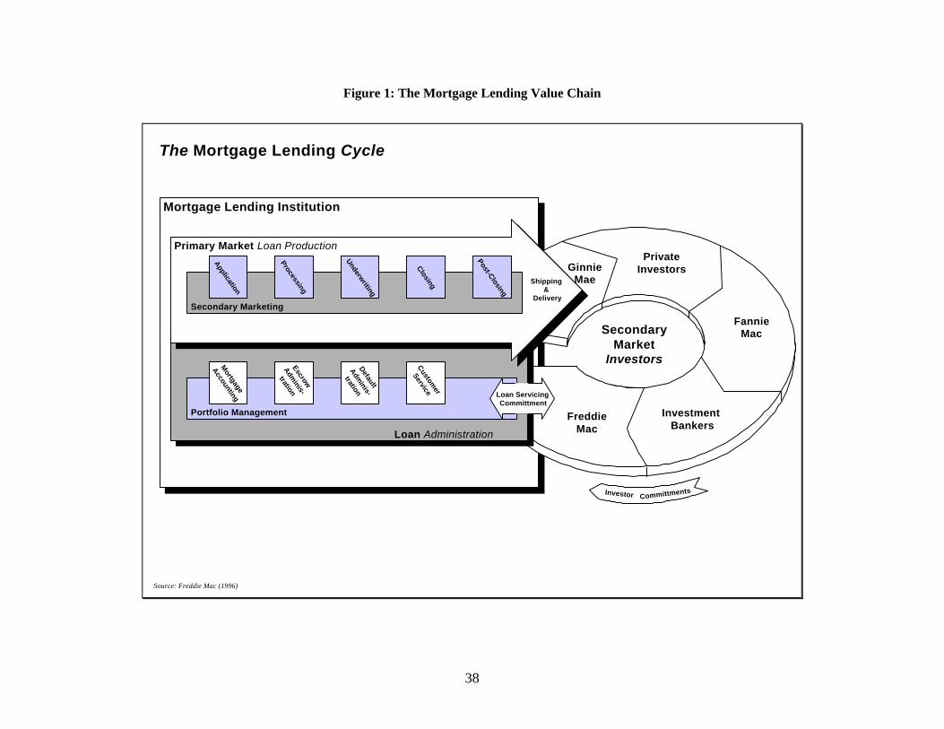
38

Figure 1: The Mortgage Lending Value Chain

FreddieMac

Investment Bankers

FannieMac

PrivateInvestors

text

Loan Administration

Mortgage Lending Institution

GinnieMae

Primary Market Loan Production

Secondary Marketing

Application

Processing

Underwriting

Closing

Post-Closing

Shipping &

Delivery

SecondaryMarket

Investors

Portfolio Management

Mortgage

Accounting

Escrow

Adminis-

tration

Default

Adminis-

tration

Customer

Service

Source: Freddie Mac (1996)

The Mortgage Lending Cycle

Loan Servicing Committment

Investor Committments

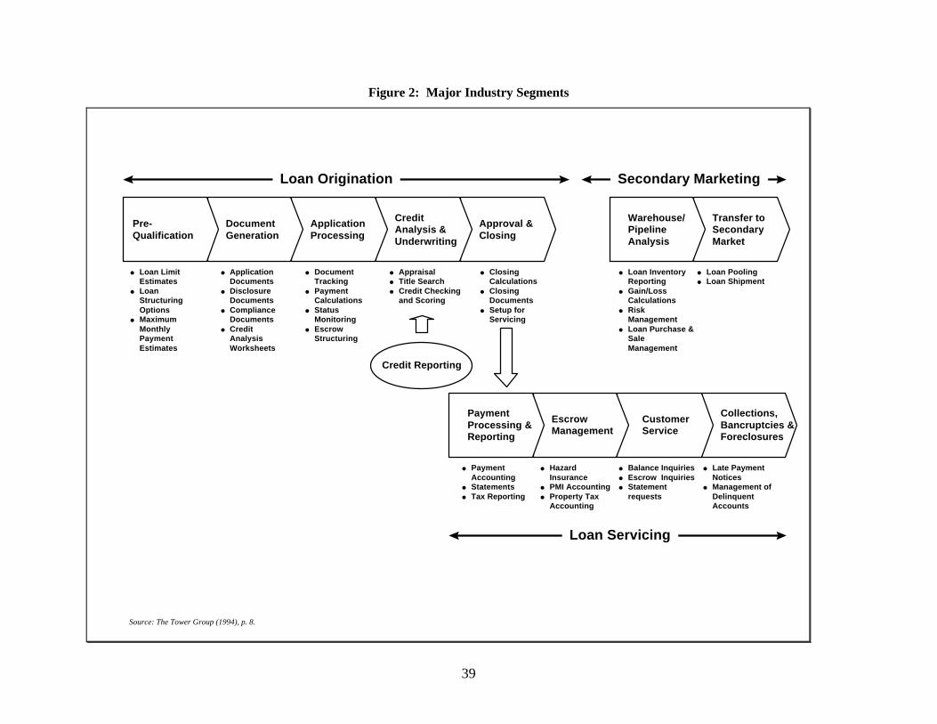
39

Figure 2: Major Industry Segments

Transfer to Secondary Market

Warehouse/Pipeline Analysis

Approval &Closing

Credit Analysis & Underwriting

ApplicationProcessing

Document Generation

Pre-Qualification

Collections,Bancruptcies &Foreclosures

Customer Service

Escrow Management

PaymentProcessing &Reporting

Credit Reporting

Loan Servicing

Secondary MarketingLoan Origination

Source: The Tower Group (1994), p. 8.

l Loan LimitEstimates

l LoanStructuringOptions

l MaximumMonthlyPaymentEstimates

l ApplicationDocuments

l DisclosureDocuments

l ComplianceDocuments

l CreditAnalysisWorksheets

l DocumentTracking

l PaymentCalculations

l StatusMonitoring

l EscrowStructuring

l Appraisall Title Searchl Credit Checking

and Scoring

l ClosingCalculations

l ClosingDocuments

l Setup forServicing

l PaymentAccounting

l Statementsl Tax Reporting

l HazardInsurance

l PMI Accountingl Property Tax

Accounting

l Balance Inquiriesl Escrow Inquiriesl Statement

requests

l Late PaymentNotices

l Management ofDelinquentAccounts

l Loan InventoryReporting

l Gain/LossCalculations

l RiskManagement

l Loan Purchase &SaleManagement

l Loan Poolingl Loan Shipment

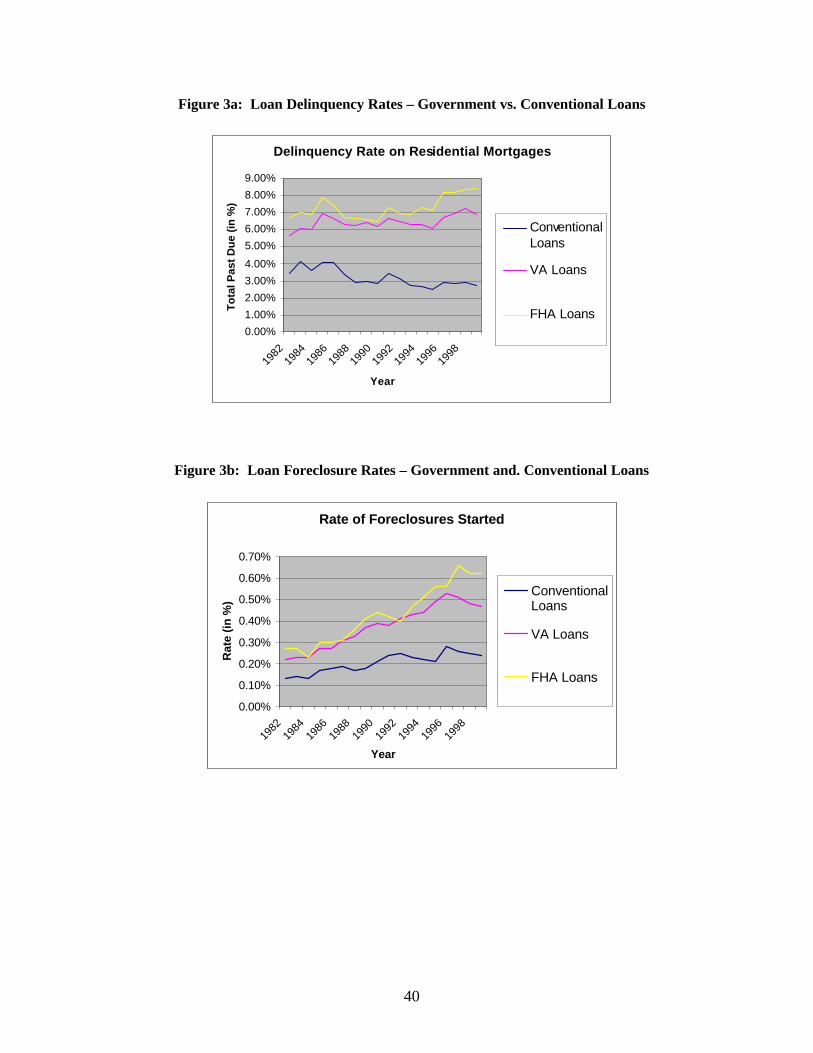
40

Figure 3a: Loan Delinquency Rates – Government vs. Conventional Loans

Delinquency Rate on Residential Mortgages

0.00%

1.00%

2.00%

3.00%

4.00%

5.00%

6.00%

7.00%

8.00%

9.00%

1982

1984

1986

1988

1990

1992

1994

1996

1998

Year

To

tal P

ast

Du

e (i

n %

)ConventionalLoans

VA Loans

FHA Loans

Figure 3b: Loan Foreclosure Rates – Government and. Conventional Loans

Rate of Foreclosures Started

0.00%

0.10%

0.20%

0.30%

0.40%

0.50%

0.60%

0.70%

1982

1984

1986

1988

1990

1992

1994

1996

1998

Year

Rat

e (i

n %

)

ConventionalLoans

VA Loans

FHA Loans

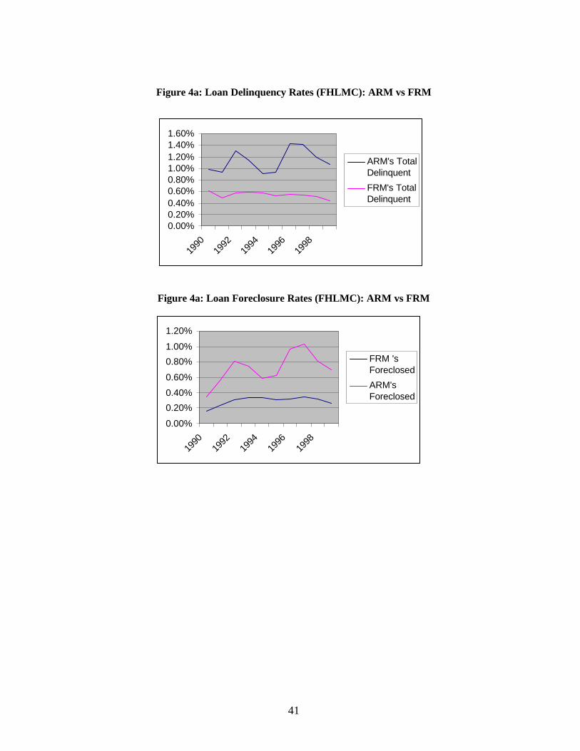
41

Figure 4a: Loan Delinquency Rates (FHLMC): ARM vs FRM

Figure 4a: Loan Foreclosure Rates (FHLMC): ARM vs FRM

0.00%0.20%0.40%0.60%0.80%1.00%1.20%1.40%1.60%

1990

1992

1994

1996

1998

ARM's TotalDelinquent

FRM's TotalDelinquent

0.00%

0.20%

0.40%

0.60%

0.80%

1.00%

1.20%

1990

1992

1994

1996

1998

FRM 'sForeclosed

ARM'sForeclosed

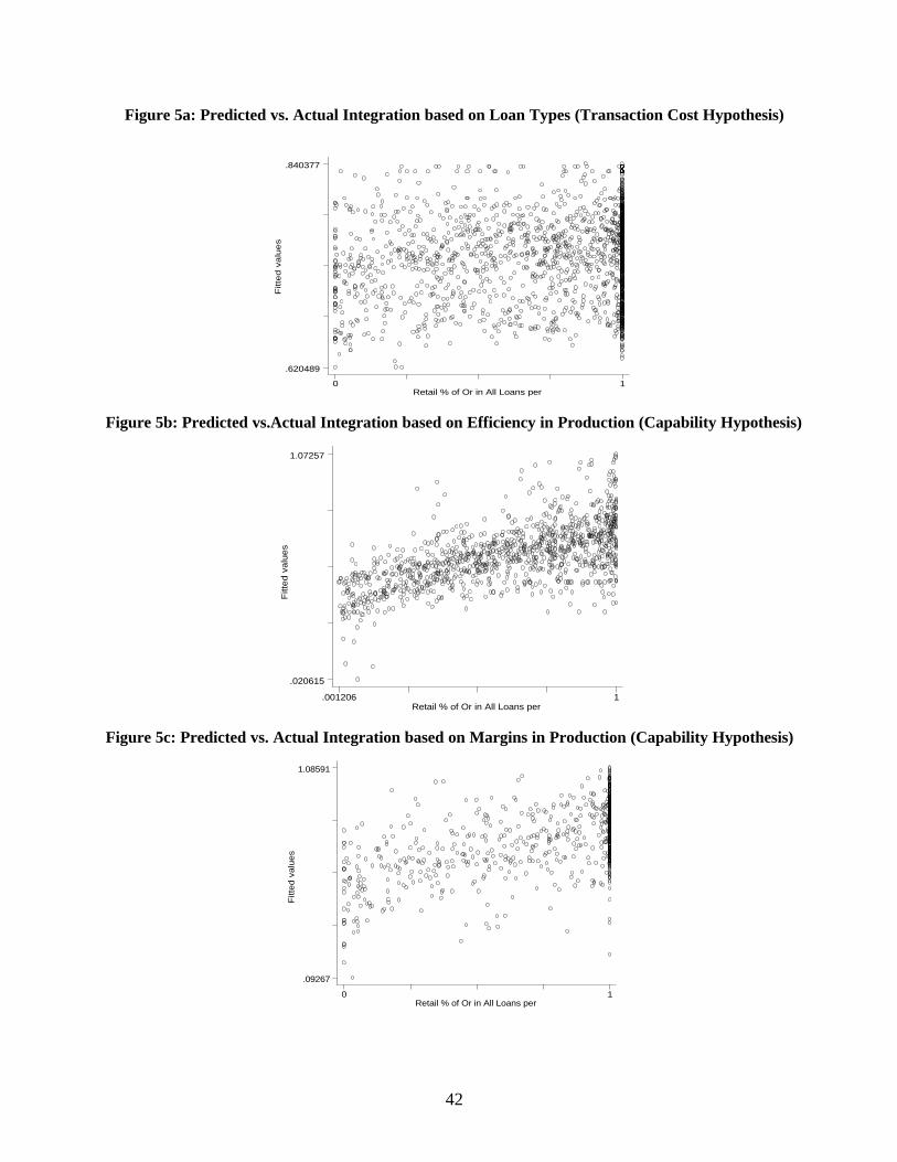
42

Figure 5a: Predicted vs. Actual Integration based on Loan Types (Transaction Cost Hypothesis)

Fitte

d v

alu

es

Retail % of Or in All Loans per 0 1

.620489

.840377

Figure 5b: Predicted vs.Actual Integration based on Efficiency in Production (Capability Hypothesis)

Fitt

ed

va

lue

s

Retail % of Or in All Loans per .001206 1

.020615

1.07257

Figure 5c: Predicted vs. Actual Integration based on Margins in Production (Capability Hypothesis)

Fitt

ed v

alu

es

Retail % of Or in All Loans per 0 1

.09267

1.08591

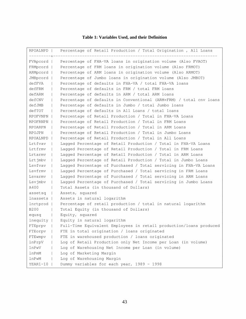
43

Table 1: Variables Used, and their Definition

RPOALNPD | Percentage of Retail Production / Total Origination , All Loans

---------+--------------------------------------------------------------------

FVApcord | Percentage of FHA-VA loans in origination volume (Also FVAOT)

FRMpcord | Percentage of FRM loans in origination volume (Also FRMOT)

ARMpcord | Percentage of ARM loans in origination volume (Also ARMOT)

JMBpcord | Percentage of Jumbo loans in origination volume (Also JMBOT)

defFVA | Percentage of defaults in FHA-VA / total FHA-VA loans

defFRM | Percentage of defaults in FRM / total FRM loans

defARM | Percentage of defaults in ARM / total ARM loans

defCNV | Percentage of defaults in Conventional (ARM+FRM) / total cnv loans

defJMB | Percentage of defaults in Jumbo / total Jumbo loans

defTOT | Percentage of defaults in All Loans / total loans

RPOFVNPN | Percentage of Retail Production / Total in FHA-VA Loans

RPOFRNPN | Percentage of Retail Production / Total in FRM Loans

RPOARPN | Percentage of Retail Production / Total in ARM Loans

RPOJPN | Percentage of Retail Production / Total in Jumbo Loans

RPOALNPD | Percentage of Retail Production / Total in All Loans

Lrtfvav | Lagged Percentage of Retail Production / Total in FHA-VA Loans

Lrtfrmv | Lagged Percentage of Retail Production / Total in FRM Loans

Lrtarmv | Lagged Percentage of Retail Production / Total in ARM Loans

Lrtjmbv | Lagged Percentage of Retail Production / Total in Jumbo Loans

Lsvfvav | Lagged Percentage of Purchased / Total servicing in FHA-VA Loans

Lsvfrmv | Lagged Percentage of Purchased / Total servicing in FRM Loans

Lsvarmv | Lagged Percentage of Purchased / Total servicing in ARM Loans

Lsvjmbv | Lagged Percentage of Purchased / Total servicing in Jumbo Loans

A400 | Total Assets (in thousand of Dollars)

assetsq | Assets, squared

lnassets | Assets in natural logarithm

lnrtprod | Percentage of retail production / total in natural logarithm

B200 | Total Equity (in thousand of Dollars)

equsq | Equity, squared

lnequity | Equity in natural logarithm

FTEprpv | Full-Time Equivalent Employees in retail production/loans produced

FTEorpv | FTE in total origination / loans originated

FTEwmpv | FTE in warehoused production / loans originated

lnPrpV | Log of Retail Production only Net Income per Loan (in volume)

lnPwV | Log of Warehousing Net Income per Loan (in volume)

lnPmM | Log of Marketing Margin

lnPwM | Log of Warehousing Margin

YEAR1-10 | Dummy variables for each year, 1989 - 1998

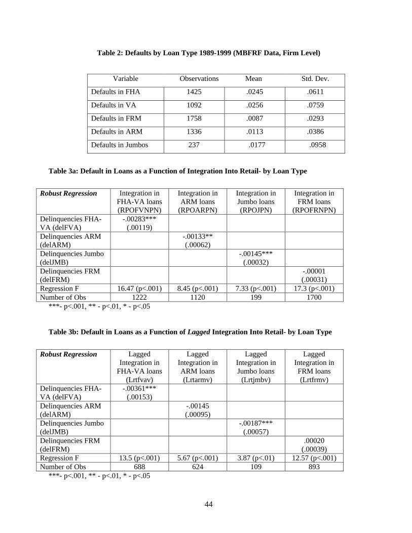
44

Table 2: Defaults by Loan Type 1989-1999 (MBFRF Data, Firm Level)

Variable Observations Mean Std. Dev.

Defaults in FHA 1425 .0245 .0611

Defaults in VA 1092 .0256 .0759

Defaults in FRM 1758 .0087 .0293

Defaults in ARM 1336 .0113 .0386

Defaults in Jumbos 237 .0177 .0958

Table 3a: Default in Loans as a Function of Integration Into Retail- by Loan Type

Robust Regression Integration inFHA-VA loans(RPOFVNPN)

Integration inARM loans

(RPOARPN)

Integration inJumbo loans(RPOJPN)

Integration inFRM loans

(RPOFRNPN)Delinquencies FHA-VA (delFVA)

-.00283***(.00119)

Delinquencies ARM(delARM)

-.00133**(.00062)

Delinquencies Jumbo(delJMB)

-.00145***(.00032)

Delinquencies FRM(delFRM)

-.00001(.00031)

Regression F 16.47 (p<.001) 8.45 (p<.001) 7.33 (p<.001) 17.3 (p<.001)Number of Obs 1222 1120 199 1700

***- p<.001, ** - p<.01, * - p<.05

Table 3b: Default in Loans as a Function of Lagged Integration Into Retail- by Loan Type

Robust Regression LaggedIntegration in

FHA-VA loans(Lrtfvav)

LaggedIntegration inARM loans(Lrtarmv)

LaggedIntegration inJumbo loans

(Lrtjmbv)

LaggedIntegration inFRM loans(Lrtfrmv)

Delinquencies FHA-VA (delFVA)

-.00361***(.00153)

Delinquencies ARM(delARM)

-.00145(.00095)

Delinquencies Jumbo(delJMB)

-.00187***(.00057)

Delinquencies FRM(delFRM)

.00020(.00039)

Regression F 13.5 (p<.001) 5.67 (p<.001) 3.87 (p<.01) 12.57 (p<.001)Number of Obs 688 624 109 893

***- p<.001, ** - p<.01, * - p<.05

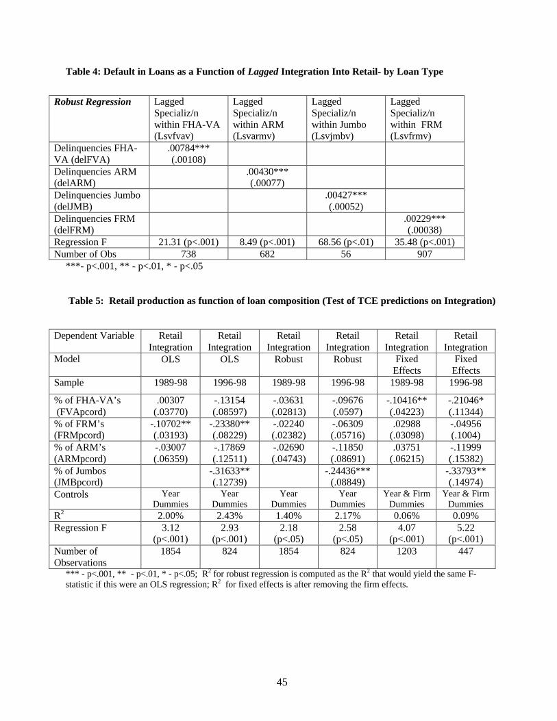
45

Table 4: Default in Loans as a Function of Lagged Integration Into Retail- by Loan Type

Robust Regression LaggedSpecializ/nwithin FHA-VA(Lsvfvav)

LaggedSpecializ/nwithin ARM(Lsvarmv)

LaggedSpecializ/nwithin Jumbo(Lsvjmbv)

LaggedSpecializ/nwithin FRM(Lsvfrmv)

Delinquencies FHA-VA (delFVA)

.00784***(.00108)

Delinquencies ARM(delARM)

.00430***(.00077)

Delinquencies Jumbo(delJMB)

.00427***(.00052)

Delinquencies FRM(delFRM)

.00229***(.00038)

Regression F 21.31 (p<.001) 8.49 (p<.001) 68.56 (p<.01) 35.48 (p<.001)Number of Obs 738 682 56 907

***- p<.001, ** - p<.01, * - p<.05

Table 5: Retail production as function of loan composition (Test of TCE predictions on Integration)

Dependent Variable RetailIntegration

RetailIntegration

RetailIntegration

RetailIntegration

RetailIntegration

RetailIntegration

Model OLS OLS Robust Robust FixedEffects

FixedEffects

Sample 1989-98 1996-98 1989-98 1996-98 1989-98 1996-98

% of FHA-VA’s (FVApcord)

.00307(.03770)

-.13154(.08597)

-.03631(.02813)

-.09676(.0597)

-.10416**(.04223)

-.21046*(.11344)

% of FRM’s(FRMpcord)

-.10702**(.03193)

-.23380**(.08229)

-.02240(.02382)

-.06309(.05716)

.02988(.03098)

-.04956(.1004)

% of ARM’s(ARMpcord)

-.03007(.06359)

-.17869(.12511)

-.02690(.04743)

-.11850(.08691)

.03751(.06215)

-.11999(.15382)

% of Jumbos(JMBpcord)

-.31633**(.12739)

-.24436***(.08849)

-.33793**(.14974)

Controls YearDummies

YearDummies

YearDummies

YearDummies

Year & FirmDummies

Year & FirmDummies

R2 2.00% 2.43% 1.40% 2.17% 0.06% 0.09%Regression F 3.12

(p<.001)2.93

(p<.001)2.18

(p<.05)2.58

(p<.05)4.07

(p<.001)5.22

(p<.001)Number ofObservations

1854 824 1854 824 1203 447

*** - p<.001, ** - p<.01, * - p<.05; R2 for robust regression is computed as the R2 that would yield the same F-statistic if this were an OLS regression; R2 for fixed effects is after removing the firm effects.

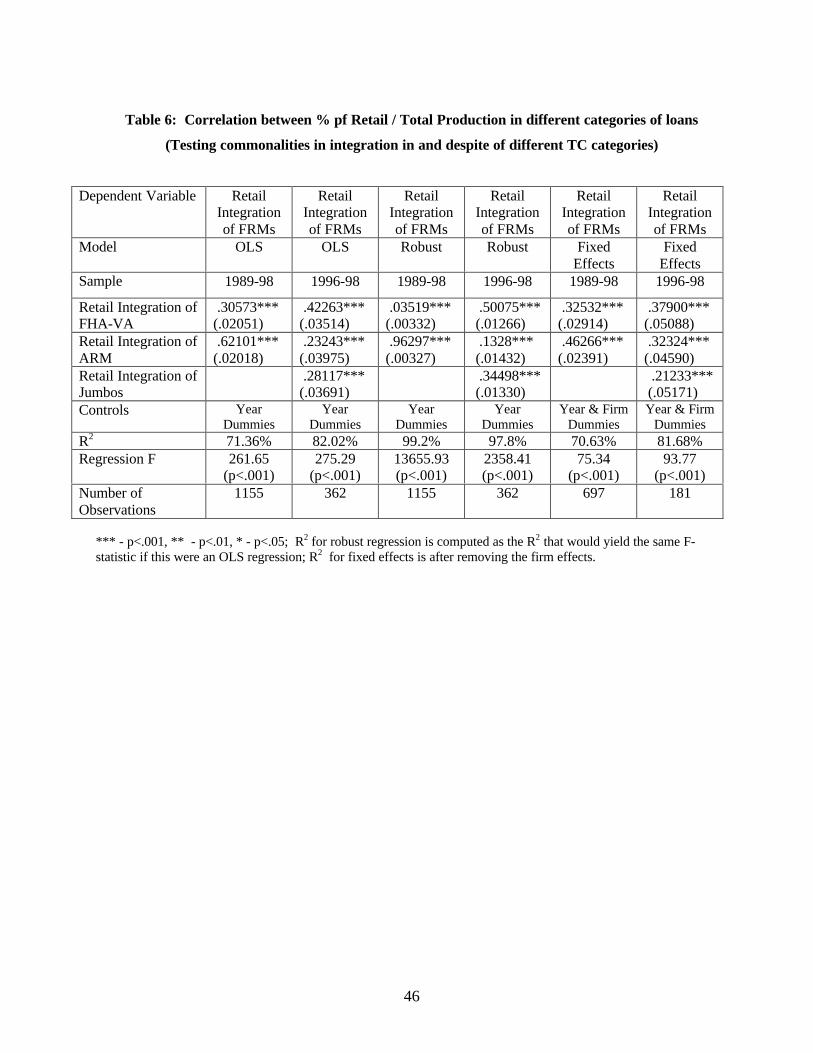
46

Table 6: Correlation between % pf Retail / Total Production in different categories of loans

(Testing commonalities in integration in and despite of different TC categories)

Dependent Variable RetailIntegrationof FRMs

RetailIntegrationof FRMs

RetailIntegrationof FRMs

RetailIntegrationof FRMs

RetailIntegrationof FRMs

RetailIntegrationof FRMs

Model OLS OLS Robust Robust FixedEffects

FixedEffects

Sample 1989-98 1996-98 1989-98 1996-98 1989-98 1996-98

Retail Integration ofFHA-VA

.30573***(.02051)

.42263***(.03514)

.03519***(.00332)

.50075*** (.01266)

.32532***(.02914)

.37900***(.05088)

Retail Integration ofARM

.62101***(.02018)

.23243***(.03975)

.96297***(.00327)

.1328*** (.01432)

.46266***(.02391)

.32324***(.04590)

Retail Integration ofJumbos

.28117***(.03691)

.34498*** (.01330)

.21233*** (.05171)

Controls YearDummies

YearDummies

YearDummies

YearDummies

Year & FirmDummies

Year & FirmDummies

R2 71.36% 82.02% 99.2% 97.8% 70.63% 81.68%Regression F 261.65

(p<.001)275.29

(p<.001)13655.93(p<.001)

2358.41(p<.001)

75.34(p<.001)

93.77(p<.001)

Number ofObservations

1155 362 1155 362 697 181

*** - p<.001, ** - p<.01, * - p<.05; R2 for robust regression is computed as the R2 that would yield the same F-statistic if this were an OLS regression; R2 for fixed effects is after removing the firm effects.

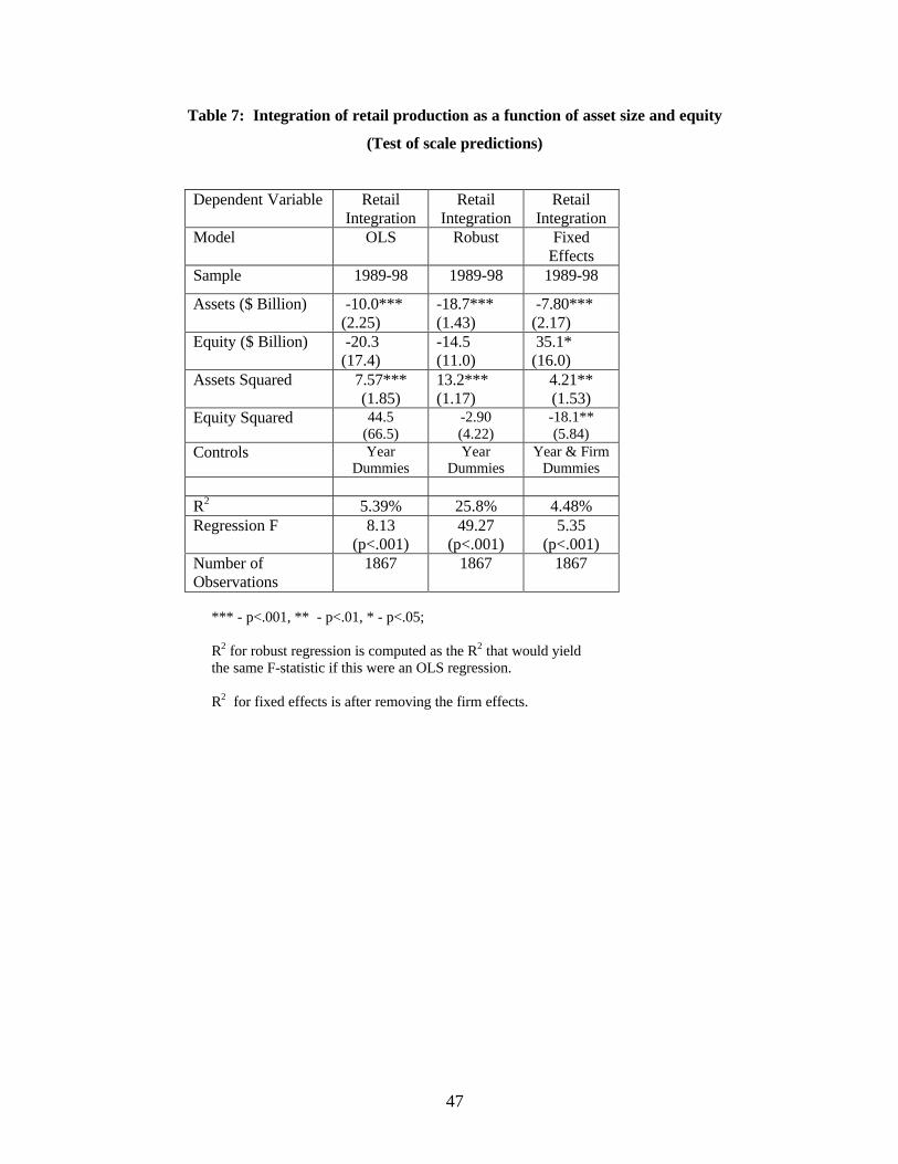
47

Table 7: Integration of retail production as a function of asset size and equity

(Test of scale predictions)

Dependent Variable RetailIntegration

RetailIntegration

RetailIntegration

Model OLS Robust FixedEffects

Sample 1989-98 1989-98 1989-98

Assets ($ Billion) -10.0***(2.25)

-18.7***(1.43)

-7.80***(2.17)

Equity ($ Billion) -20.3(17.4)

-14.5(11.0)

35.1*(16.0)

Assets Squared 7.57***(1.85)

13.2***(1.17)

4.21**(1.53)

Equity Squared 44.5(66.5)

-2.90(4.22)

-18.1**(5.84)

Controls YearDummies

YearDummies

Year & FirmDummies

R2 5.39% 25.8% 4.48%Regression F 8.13

(p<.001)49.27

(p<.001)5.35

(p<.001)Number ofObservations

1867 1867 1867

*** - p<.001, ** - p<.01, * - p<.05;

R2 for robust regression is computed as the R2 that would yieldthe same F-statistic if this were an OLS regression.

R2 for fixed effects is after removing the firm effects.

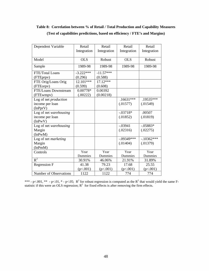
48

Table 8: Correlation between % of Retail / Total Production and Capability Measures

(Test of capabilities predictions, based on efficiency / FTE’s and Margins)

Dependent Variable RetailIntegration

RetailIntegration

RetailIntegration

RetailIntegration

Model OLS Robust OLS Robust

Sample 1989-98 1989-98 1989-98 1989-98

FTE/Total Loans(FTEprpv)

-3.222***(0.296)

-11.57***(0.588)

FTE Orig/Loans Orig(FTEorpv)

12.101***(0.599)

17.12***(0.608)

FTE/Loans Downstream(FTEwmpv)

0.00778*(.00222)

0.00392(0.00218)

Log of net productionincome per loan(lnPprV)

.16631***(.01577)

.19535***(.01549)

Log of net warehousingincome per loan(lnPwV)

-.03718*(.01852)

.00507(.01819)

Log of net warehousingMargin(lnPwM)

-.03941(.02316)

-.05883*(.02275)

Log of net marketingMargin(lnPmM)

-.09349***(.01404)

-.10362***(.01379)

Controls YearDummies

YearDummies

YearDummies

YearDummies

R2 30.91% 46.06% 21.91% 31.89%Regression F 41.38

(p<.001)79.23

(p<.001)17.68

(p<.001)25.55

(p<.001)Number of Observations 1122 1122 774 774

*** - p<.001, ** - p<.01, * - p<.05; R2 for robust regression is computed as the R2 that would yield the same F-statistic if this were an OLS regression; R2 for fixed effects is after removing the firm effects.

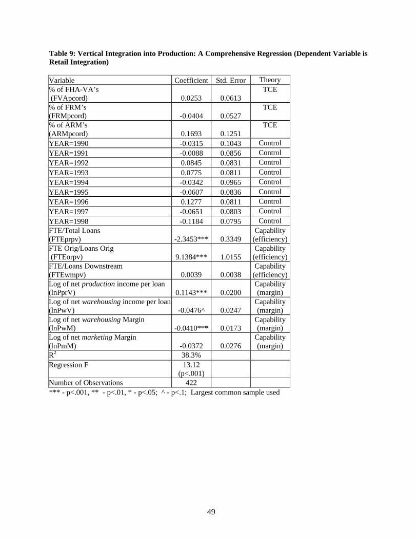
49

Table 9: Vertical Integration into Production: A Comprehensive Regression (Dependent Variable isRetail Integration)

Variable Coefficient Std. Error Theory% of FHA-VA’s (FVApcord) 0.0253 0.0613

TCE

% of FRM’s(FRMpcord) -0.0404 0.0527

TCE

% of ARM’s(ARMpcord) 0.1693 0.1251

TCE

YEAR=1990 -0.0315 0.1043 ControlYEAR=1991 -0.0088 0.0856 ControlYEAR=1992 0.0845 0.0831 ControlYEAR=1993 0.0775 0.0811 ControlYEAR=1994 -0.0342 0.0965 ControlYEAR=1995 -0.0607 0.0836 ControlYEAR=1996 0.1277 0.0811 ControlYEAR=1997 -0.0651 0.0803 ControlYEAR=1998 -0.1184 0.0795 ControlFTE/Total Loans(FTEprpv) -2.3453*** 0.3349

Capability(efficiency)

FTE Orig/Loans Orig (FTEorpv) 9.1384*** 1.0155

Capability(efficiency)

FTE/Loans Downstream(FTEwmpv) 0.0039 0.0038

Capability(efficiency)

Log of net production income per loan(lnPprV) 0.1143*** 0.0200

Capability(margin)

Log of net warehousing income per loan(lnPwV) -0.0476^ 0.0247

Capability(margin)

Log of net warehousing Margin(lnPwM) -0.0410*** 0.0173

Capability(margin)

Log of net marketing Margin(lnPmM) -0.0372 0.0276

Capability(margin)

R2 38.3%Regression F 13.12

(p<.001)Number of Observations 422*** - p<.001, ** - p<.01, * - p<.05; ^ - p<.1; Largest common sample used