vibration and rattle mitigationweb.mit.edu/aeroastro/partner/reports/proj1/proj1.6report.pdf ·...
TRANSCRIPT
Partnership for AiR Transportation Noise and Emissions ReductionAn FAA/NASA/Transport Canada-sponsored Center of Excellence
Vibration and Rattle Mitigation
PARTNER Project 1.6 report
prepared by
Daniel H. Robinson, Robert J. Bernhard, Luc G. Mongeau
January 2008
REPORT N0. PARTNER-COE-2008-004

VIBRATION AND RATTLE MITIGATION PARTNER Project 1.6 Report
January 2008
Prepared by: Daniel Robinson
Robert Bernhard, Luc G. Mongeau
Purdue University
PARTNER Report No.: PARTNER-COE-2008-004
Any opinions, findings, and conclusions or recommendations expressed in this material are of the authors and do not necessarily reflect the views of the FAA, NASA, or
Transport Canada.
The Partnership for AiR Transportation Noise and Emissions Reduction — PARTNER — is a leading aviation cooperative research organization, and an FAA/NASA/Transport Canada-sponsored Center of Excellence. PARTNER fosters breakthrough technological, operational, policy, and workforce advances for the betterment of mobility, economy, national security, and the environment. The organization's operational headquarters is at the Massachusetts Institute of Technology.
The Partnership for AiR Transportation Noise and Emissions Reduction Massachusetts Institute of Technology, 77 Massachusetts Avenue, 37-395
Cambridge, MA 02139 USA http://www.partner.aero
PARTNER Project 1.6 Report: Vibration and Rattle Mitigation
Daniel H. Robinson
Dr. Robert J. Bernhard and Dr. Luc G. Mongeau
Purdue University
2
TABLE OF CONTENTS Page
1 INTRODUCTION ...................................................................................................................3 2 ANALYTICAL RATTLE MODELS......................................................................................5
2.1 Non-Resonant Rattle Systems..................................................................................5 2.1.a Case 1: Object on a Vibrating Floor ........................................................................7 2.1.b Case 2: Beam Leaning on the Corner of Vibrating Floor........................................9 2.1.c Case 3: Beam Leaning on the Corner of Vibrating Wall.......................................10 2.1.d Summary of Rattle Thresholds for Non-Resonant Systems ..................................12
2.2 Resonant Rattle Systems........................................................................................12 2.2.a Case 4: Object on a Flexible Floor ........................................................................15 2.2.b Case 5: Effects of Preload......................................................................................20 2.2.c Case 6: Effects of Preload and Flexible Floor .......................................................25
3 EXPERIMENTAL RATTLE STUDY ..................................................................................40 3.1 Objective ................................................................................................................40 3.2 Test Method ...........................................................................................................40 3.3 Mobility Analysis of Rattle-Prone Windows.........................................................43 3.4 Experimental Results .............................................................................................46
3.4.a Swept Sine Excitation............................................................................................48 3.4.b Aircraft Take-Off Excitation..................................................................................53 3.4.c Random Excitation.................................................................................................56
4 SUMMARY AND CONCLUSIONS ....................................................................................59 5 LIST OF REFERENCES.......................................................................................................63 6 APPENDICES .......................................................................................................................64
6.1 Appendix A: Experimental plots of rattle study ...................................................65 6.1.a Plots of Lower East (LE) window .........................................................................65 6.1.b Plots of Lower West (LW) window.......................................................................78 6.1.c Plots of Upper East (UE) window .........................................................................91 6.1.d Plots of Upper West (UW) window.....................................................................104
6.2 Appendix B: Measured Window Rattle Thresholds ............................................117
3
1 INTRODUCTION
High levels of low frequency noise are created by aircraft during take-off and landing. A
by-product of low frequency sound incident on a building façade is the excitation of structures
within the building into vibrations. Such acoustically-induced structural vibrations may be
imperceptible, but they may cause rattle. Rattle is caused by the intermittent loss of contact
between two bodies due to vibration [1]. Rattle causes secondary noise emissions, which are
often perceived as annoying [2]. Investigation of the mechanisms leading to rattle onset and the
development of rattle mitigation strategies are needed to reduce rattle emissions, and the
associated annoyance.
Analytical models of idealized systems which have the potential to rattle were developed
in this investigation. Comparisons were made between model predictions and results from
experiments. From the analytical models, rattle onset thresholds were determined for simple
models of various household components such as: window systems, wall hangings, door latches
and bric-a-brac. The analytical rattle onset models provide guidelines for design to mitigate
rattle.
The analytical models are lumped-parameter, single-degree-of-freedom models of
elements typically found in homes. The models are divided into two classes: resonant and non-
resonant systems. Previous research conducted by others [3]-[8] have used non-resonant models
to describe rattle. These models describe some practical systems. However, many systems rattle
because of resonant properties. It is assumed that the response of multi-degree-of-freedom
systems may be modeled as a superposition of single-degree-of-freedom systems. This
investigation will focus only on single degree of freedom systems. Rattle criterion are developed
for various excitation sources including harmonic base motion and forced excitation. These
criteria include the rattle onset threshold and the rattle bandwidth, which is a feature of resonant
systems.

4
An in-situ experiment was conducted at the Ray W. Herrick Laboratories. Four windows
known to be susceptible to rattle were excited via high-fidelity playback of three high-amplitude,
low-frequency noise signals. The signals included pre-recorded aircraft take-off noise, a swept
sine signal, and random noise. The vibration and acoustic response of each of the windows was
measured to determine the relationship between frequency and acceleration level for onset of
rattle and qualitatively validate the behavior predicted by the analytical models.

5
2 ANALYTICAL RATTLE MODELS
Six simple models were developed which include cases with and without preload. Rattle
criteria were developed for various excitation mechanisms, including harmonic base motion and
harmonic forced excitation. For harmonic base motion, the rattle onset threshold was established
in terms of base acceleration magnitude. For an acoustically forced excitation, the rattle onset
threshold was expressed in terms of the incident sound pressure amplitude. The criteria
considered included the rattle onset threshold and the rattle bandwidth, the latter being a feature
that is unique to resonant systems.
To determine rattle onset, the linear Newtonian equations of motion are solved to find the
condition where the contact force between the rattle object and the vibrating base becomes zero
at an extrema of harmonic excitation. When the contact force becomes zero, contact will be lost
between the rattling object and the vibrating base for a short period of time. For excitation
amplitudes in excess of the rattle onset threshold loss of contact will occur for a greater time.
The repeated re-establishment of contact is the cause for rattle noise. Rattle duration, intensity,
or motion was not investigated; these phenomena involve the use of non-linear models. The
prediction of the first loss of contact using a linear model was deemed indicative of repeated loss
of contact, and thus of the rattle onset threshold.
2.1 Non-Resonant Rattle Systems
Schematics of the non-resonant rattle systems are shown in Table 2.1. Three non-
resonant models, Cases 1 through 3, were considered. Each involves one rigid body in contact
with a vibrating base. Case 1 is an idealization of an object lying on a vibrating floor or shelf.
Case 1 is similar to Hubbard’s normal excitation model [1]. The excitation is assumed to be in

6
the direction normal to the base of the rigid object. Cases 2 and 3 describe objects leaning
against a wall. Cases 2 and 3 are similar to the models of Carden/Mayes [6] and Sutherland [47-
48] for objects that lean at an angle against a vibrating surface. For Case 2, the rattling system is
excited vertically through the base, while in Case 3, the rattling system is excited horizontally
through the wall.
For each case the rattle onset threshold was defined as the acceleration amplitude, Ab, at
which contact was lost between the mass and the vibrating surface.
Table 2.1: Non-resonant rattle systems.
Case Description Example Schematic
1 Object on a vibrating floor
Alarm clock, lamp, decorative element,…
2 Beam leaning on corner of vibrating floor
Picture frame, bric-a-brac,…
3 Beam leaning on corner of vibrating wall
Picture frame, bric-a-brac,…
7
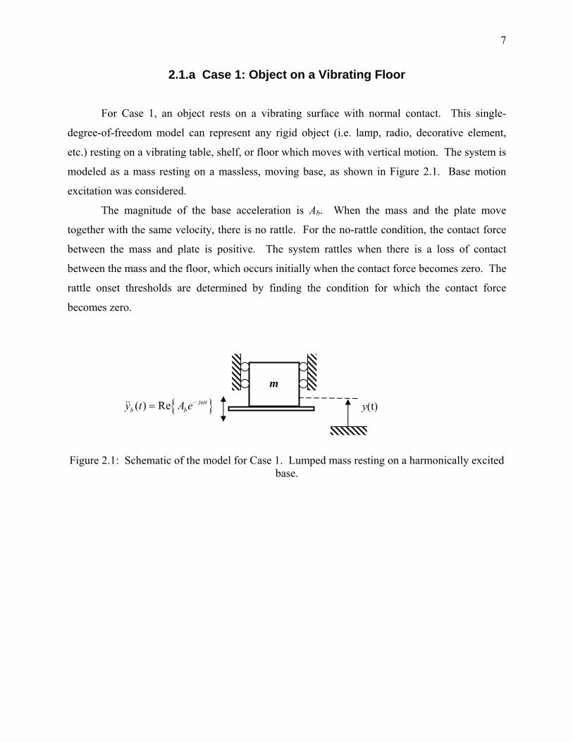
2.1.a Case 1: Object on a Vibrating Floor
For Case 1, an object rests on a vibrating surface with normal contact. This single-
degree-of-freedom model can represent any rigid object (i.e. lamp, radio, decorative element,
etc.) resting on a vibrating table, shelf, or floor which moves with vertical motion. The system is
modeled as a mass resting on a massless, moving base, as shown in Figure 2.1. Base motion
excitation was considered.
The magnitude of the base acceleration is Ab. When the mass and the plate move
together with the same velocity, there is no rattle. For the no-rattle condition, the contact force
between the mass and plate is positive. The system rattles when there is a loss of contact
between the mass and the floor, which occurs initially when the contact force becomes zero. The
rattle onset thresholds are determined by finding the condition for which the contact force
becomes zero.
m
Figure 2.1: Schematic of the model for Case 1. Lumped mass resting on a harmonically excited base.
y(t) { }j( ) Re tb by t A e ω−=
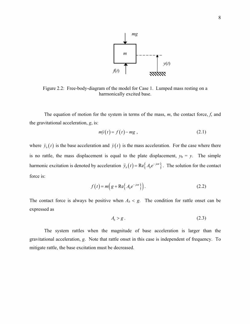
8
mg
m
y(t) f(t)
Figure 2.2: Free-body-diagram of the model for Case 1. Lumped mass resting on a harmonically excited base.
The equation of motion for the system in terms of the mass, m, the contact force, f, and
the gravitational acceleration, g, is:
( ) ( )my t f t mg= − , (2.1)
where ( )by t is the base acceleration and ( )y t is the mass acceleration. For the case where there
is no rattle, the mass displacement is equal to the plate displacement, yb = y. The simple
harmonic excitation is denoted by acceleration ( ) { }Re j tb by t A e ω−= . The solution for the contact
force is:
( ) { }( )Re j tbf t m g A e ω−= + . (2.2)
The contact force is always be positive when Ab < g. The condition for rattle onset can be
expressed as
. (2.3) bA g>
The system rattles when the magnitude of base acceleration is larger than the
gravitational acceleration, g. Note that rattle onset in this case is independent of frequency. To
mitigate rattle, the base excitation must be decreased.
9
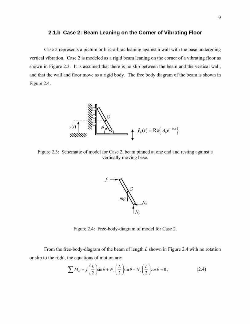
2.1.b Case 2: Beam Leaning on the Corner of Vibrating Floor
Case 2 represents a picture or bric-a-brac leaning against a wall with the base undergoing
vertical vibration. Case 2 is modeled as a rigid beam leaning on the corner of a vibrating floor as
shown in Figure 2.3. It is assumed that there is no slip between the beam and the vertical wall,
and that the wall and floor move as a rigid body. The free body diagram of the beam is shown in
Figure 2.4.
G
θ
Figure 2.3: Schematic of model for Case 2, beam pinned at one end and resting against a vertically moving base.
Figure 2.4: Free-body-diagram of model for Case 2.
From the free-body-diagram of the beam of length L shown in Figure 2.4 with no rotation
or slip to the right, the equations of motion are:
sin sin cos 02 2 2G x yL L LM f N Nθ θ⎛ ⎞ ⎛ ⎞ ⎛ ⎞= + −⎜ ⎟ ⎜ ⎟ ⎜ ⎟
⎝ ⎠ ⎝ ⎠ ⎝ ⎠∑ θ = , (2.4)
{ }( ) Re j tb by t A e ω−=
y(t)
f G
mg Nx
Ny

10
0x xF f N= − =∑ , (2.5)
y yF N m Gg my= − =∑ . (2.6)
The vertical acceleration of the object when rattle does not occur is
{ }Re j tG by A e ω−= . (2.7)
From equation (2.6) and (2.7),
{ }( )Re j ty bN m g A e ω−= + . (2.8)
After substitution of equation (2.4) into (2.5),
2 sin cos 0yf Nθ θ− = , (2.9)
where, sin2 2 tcosyN f fθ anθ
θ= = . (2.10)
From equation (2.8), the following equation is obtained,
( ){ }( )Re
2tan
j tbm g A e
f tω
θ
−+= . (2.11)
The contact force is always positive for Ab < g. Thus, rattle will occur when:
. (2.12) bA g>
The rattle onset threshold is independent of frequency and angle, θ. To mitigate rattle,
the magnitude of the base excitation must be decreased.
2.1.c Case 3: Beam Leaning on the Corner of Vibrating Wall
Case 3 is similar to Case 2. However, for case 3 the system is vibrating in the horizontal
direction as shown in Figure 2.5.

11
Figure 2.5: Schematic of model for Case 3, beam pinned at one end and resting against a horizontally moving base.
Figure 2.6: Free body diagram of model for Case 3.
The equations of motions are derived from the free-body-diagram of the object of length
L shown in Figure 2.6. As with Case 2 there is no rotation or slip at the contact between the base
and beam.
sin cos cos 02f x yLM LN mg LNθ θ⎛ ⎞= + −⎜ ⎟
⎝ ⎠∑ θ =
G
, (2.13)
x xF f N mx= − =∑ , (2.14)
0y yF N mg= − =∑ . (2.15)
The horizontal acceleration of the object when rattle does not occur is
{ }Re j tG bx A e ω−= . (2.16)
x(t)
G
θ { }j( ) Re tbx t A e ω−=
f G
mg Nx
Ny

12
Substitution of equation (2.15) into (2.13) yields:
2 tanx
mgNθ
= . (2.17)
From equation (2.14), (2.16) and (2.17),
( ) { }Re2 tan
j tb
gf t m A e ω
θ−⎛= +⎜
⎝ ⎠⎞⎟ . (2.18)
Thus, rattle occurs when:
2 tanb
gAθ
> . (2.19)
For increasing θ, less base excitation, Ab, is needed to cause rattle. Therefore, to mitigate rattle,
the angle with respect to the floor should be minimized.
2.1.d Summary of Rattle Thresholds for Non-Resonant Systems
Hubbard predicted that an object resting on a vibrating floor rattles when the floor
acceleration amplitudes exceeded gravity [3]. Case 1 illustrates this behavior. However, from
experimental data Hubbard noticed that rattle can occur for acceleration amplitudes less than
gravity. Resonant rattle systems may explain this behavior. In both the Clevenson [5] and the
Carden/Mayes studies [6], it was found that the rattle onset threshold is inversely proportional to
the angle of the leaning object. The analysis of Case 3 supports this conclusion for horizontal
excitation of the base. However, if the base is excited vertically, the lean angle does not affect
the rattle onset threshold, as shown in equation (2.12).
2.2 Resonant Rattle Systems
The resonant rattle system models are extensions of the non-resonant system models,
accounting for the added effects of stiffness, damping and preload. Resonant systems are
frequency dependent. The rattle onset threshold is related to both the base excitation amplitude

13
and frequency. Dissipative elements were treated as structural damping with complex stiffness,
k(1+jγ), where γ is the structural damping coefficient. Structural damping coefficients for
typical solid structures (wood, glass, metal, etc…) are small (γ ranges from 0.0001 to 0.03).
A steady-state harmonic base acceleration excitation of amplitude, Ab, was considered for
Case 4, and a harmonic base displacement excitation of amplitude, Yb, was considered for Cases
5 and 6. The motion of the system was assumed to respond linearly as long as the contact force
is positive. Rattle onset thresholds were determined analytically by solving for the conditions for
which the contact force, f, between the two objects first goes to zero, . It was assumed
that this condition occurs at a peak acceleration condition. Expressions for the complex contact
force coefficient were obtained in terms of complex displacement amplitudes. The complex
coefficients were restated into a time factor of the form
0f →
( )j te ω φ− − . The real part of this term
oscillates between 1 and -1. Rattle onset thresholds were derived for steady-state motion by
making the complex time factor equal to 1 or -1. The results were verified by performing time-
marching simulations of the contact force for each resonant system to validate that the rattle
thresholds established by this procedure occur as expected for transient conditions.
For the time-marching simulations, the Runge-Kutta method was used to numerically
approximate the ordinary differential equations that describe the contact force equation. For a
given set of mass, stiffness, and damping parameters, the response was calculated for a range of
excitation amplitudes and frequencies above and below the predicted rattle onset threshold. The
time-marching simulations were evaluated at extremes of typical parameter values. The values
of the parameters were selected to bound the range of typical properties of housing components.
Natural frequency, ωn, values of 0.001 rad/s and 100 rad/s were evaluated, representing the
bounds of mass and stiffness combinations for mass values of 0.001 kg and 100 kg; and stiffness
values of 0.01 N/m and 1000 N/m. Structural damping, γ, was evaluated for values of 0.0001
and 0.1. Preload was a parameter for Case 5 and 6 resonant rattle systems. The preload values
evaluated for these systems was yp,min and yp,min+10, where yp,min is the minimum preload required
to maintain contact between two objects at rest. The excitation acceleration amplitude, Ab, was
evaluated for three values; 0 m/s2, 1 m/s2, and 10 m/s2 for Case 4. The excitation displacement
amplitude, Yb, was evaluated for three values; 0 m, 0.001 m, and 0.01 m for Cases 5 and 6. The
time-marching simulation were evaluated at five excitation frequency, ω, values;

14
0.1ωn, 0.9ωn, ωn, 1.1ωn, and 10ωn. The time marching simulations were evaluated for a
combination of all selected parameter values for each of the three resonant rattle systems. A
total of 41 time-marching simulations were evaluated for Case 4 and 81 simulations each for
Cases 5 and 6. It was found that the contact force for each of the simulations first went to zero
near the instant of peak amplitude motion. While in principle this may not always be the case,
the simulations demonstrated that for the small damping values considered, the rattle onset
thresholds could accurately be determined from steady-state solutions and that rattle first occurs
when ( ) 1j te ω φ− − = ± . The time-marching simulations also showed that the excitation amplitude
necessary to cause the loss of contact was identical to the amplitude predicted by analytical
derivation. Schematics of the three resonant rattle systems are shown in Table 2.2.

15
Table 2.2: Resonant rattle systems.
Case Description
Example Schematic
4
Object on a flexible floor vibration through the floor from the foundation or floor joists
5
Effects of pre-load lighting fixtures or door latches which are held against a surface by a spring
6
Effects of pre-load & flexible floor
window system with pre-loaded gaskets or a door in a door frame
yp
2.2.a Case 4: Object on a Flexible Floor
Case 4 is a modification of Case 1. It represents an object resting freely on a flexible
floor, such as a block resting on a floor board between joists or bric-a-brac resting on a flexible
shelf. For this case, the inertial force due to gravity, g, holds the object in contact with the base.
The flexible floor is modeled as a mass-spring-damper system with masses, m1 and m2, and
yp
2ω
1ω
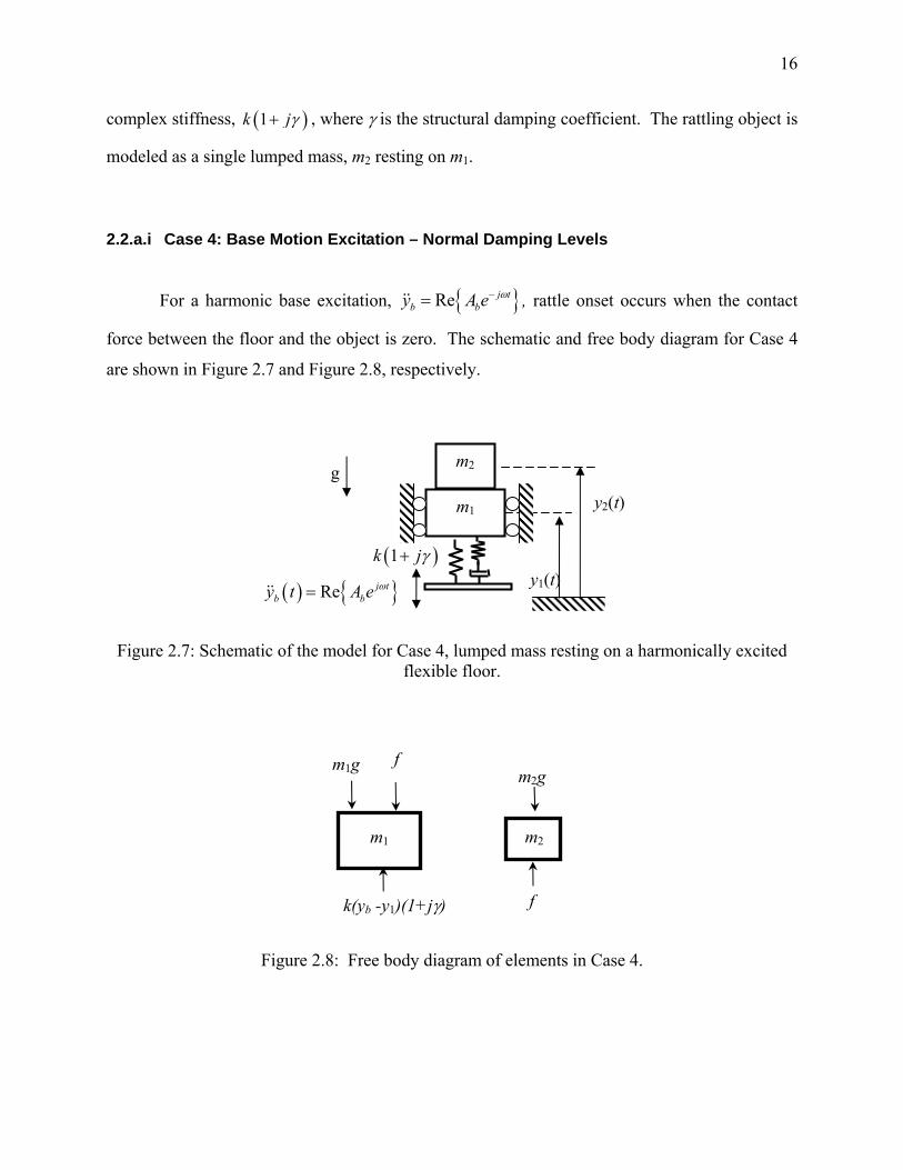
16
complex stiffness, (1k )jγ+ , where γ is the structural damping coefficient. The rattling object is
modeled as a single lumped mass, m2 resting on m1.
2.2.a.i Case 4: Base Motion Excitation – Normal Damping Levels
For a harmonic base excitation, { }Re j tb by A e ω−= , rattle onset occurs when the contact
force between the floor and the object is zero. The schematic and free body diagram for Case 4
are shown in Figure 2.7 and Figure 2.8, respectively.
m2 g
Figure 2.7: Schematic of the model for Case 4, lumped mass resting on a harmonically excited flexible floor.
Figure 2.8: Free body diagram of elements in Case 4.
m2g
m2
f
f
m1g
k(yb -y1)(1+jγ)
m1
m1
( )1k jγ+ y1(t)
y2(t)
( ) { }Re j tb by t A e ω=

17
The steady-state harmonic motion of the masses m1 and m2 is described in the complex
notation form using ( ) { }1 1Re j ty t Ae ω−= , ( ) { }1 12
1 Re j ty t A e ω
ω−= − , ( ) { }2 2Re j ty t A e ω−= and
( ) {2 2
1 Re }2j ty t A e ω
ω−= − . The motion of the vibrating base is described by ( ) { }Re j t
b by t A e ω−=
and ( ) {2
1 Re }j tby t A e ω
ω−= − b . The equations of motion are:
( ) ( ) ( )1 1 12 2Re 1 Re 1j t j tb o
k km j A e j A e ky f tω ωγ γω ω
− −⎧ ⎫⎡ ⎤ ⎧ ⎫− + = − + + − −⎨ ⎬ ⎨ ⎬⎢ ⎥⎣ ⎦ ⎩ ⎭⎩ ⎭m g , (2.20)
{ } ( )2 2 2Re j tm A e f t mω = − g , (2.21)
where f(t) is the contact force between masses. Here, yo is the static displacement of the
suspended system induced by the weight,
2o ny Mg k g ω= = , (2.22)
where 1 2M m m= + , and n k Mω = is the natural frequency of the system. For motion when
rattle does not occur, the masses move together with the same acceleration ( )1 2i.e., A A A= =
and the contact force is positive. The solution for 1 2A A A= = , is:
( ) ( )( )2
1
1b
n
A jA j
j
γω
ω ω γ
+=
⎡ ⎤− +⎣ ⎦. (2.23)
or,
( )( )
{1 2
2
22 2
1 Re1
jb
n
A A e }φγωω ω γ
−
⎧ ⎫+⎪ ⎪= ⎨ ⎬
⎡ ⎤⎪ ⎪− +⎣ ⎦⎩ ⎭
, (2.24)
where φ is the phase angle of the response with respect to the force. The acceleration of the
masses is
( )( )
( ){1 2
2
22 2
1 Re1
j tb
n
y t A e ω φγ
ω ω γ
− +
⎧ ⎫+⎪ ⎪= ⎨ ⎬
⎡ ⎤⎪ ⎪− +⎣ ⎦⎩ ⎭
} . (2.25)

18
Substitution of equation (2.25) into (2.21) yields, for contact force, f(t)
( ) ( )( )
( )( ){ }
2
1 2
2
2 22 2
1 Re1
j tb
n
f t m g y t
m g A e ω φγ
ω ω γ
− +
= +
⎛ ⎞⎧ ⎫⎜ ⎟+⎪ ⎪= +⎜ ⎟⎨ ⎬
⎡ ⎤⎜ ⎟⎪ ⎪− +⎜ ⎟⎣ ⎦⎩ ⎭⎝ ⎠
. (2.26)
Rattle onset occurs when the contact force becomes zero (f = 0), which will occur at peak
acceleration amplitudes when ( ) 1j te ω φ− + = − . Thus,
( )
1 2
2
22 2
10 1 .1
b
n
Ag
γ
ω ω γ
⎧ ⎫+⎪ ⎪= − ⎨ ⎬
⎡ ⎤⎪ ⎪− +⎣ ⎦⎩ ⎭
(2.27)
Solving equation (2.27) in terms of ( n )ω ω , rattle occurs in a frequency band defined by,
( ) ( ) ( ) ( ) ( )2 22 2 21 1 1 1b n bA g A g 2γ γ ω ω γ γ− + − < < + + − . (2.28)
For Case 4, rattle occurs in a band around the natural frequency of the system, which will be
referred to as the rattle band. A non-dimensional rattle band parameter, λ, is defined such that
( )n U L nλ ω ω ω ω ω= Δ = − , where ωU and ωL are the upper and lower rattle onset thresholds,
respectively. The lower rattle threshold, ωL, must be greater than 0 Hz. For a larger non-
dimensional rattle bandwidth, rattle occurs over a broader range of frequencies. Thus, one
design objective would be to keep the rattle bandwidth as small as possible.
The rattle bandwidth dependence on base excitation, Ab, and structural damping, γ, is
shown in Figure 2.9. The contour labels indicate the magnitude of the rattle bandwidth, λ. The
influence of damping is not significant until the structural damping factor is greater than
approximately 0.1. Thus for typical structures the effects of damping are negligible for rattle
onset. For cases where damping is negligible, equation (2.28) can be rewritten as:
( )1 b nA g A gω ω− < < +1 b . (2.29)
For configurations for which Case 4 is a reasonable model, the only strategy to minimize the
rattle bandwidth is by keeping the magnitude of the excitation small.

19
Structural Damping Factor, γ
Bas
e A
ccel
erat
ion,
A b
0.05
0.2
0.4
0.6
0.8
1
1.2
10-4
10-3
10-2
10-1
100
1010
(1/4)g
(1/2)g
(3/4)g
g
Figure 2.9: Contours of equal non-dimensional rattle bandwidth, λ, (vs. structural damping factor, γ, and base acceleration, Ab).
2.2.a.ii Case 4: Base Motion Excitation – High Damping Levels
It is of interest to determine how much damping would be necessary to prevent rattle.
When the rattle bandwidth, ( )U L nλ ω ω ω= − , is zero, the system does not rattle for any
excitation amplitude. From Figure 2.9, damping does reduce the rattle band for values of
structural damping greater than 0.1, ( )0.1γ > . The rattle bandwidth is zero for
( ){ } 1 22 1bg Aγ−
= − . (2.30)
The amount of damping necessary to prevent rattle for a given ratio of excitation
acceleration to gravity is determined from equation (2.30). The damping necessary to prevent
rattle is shown versus the ratio of gravity and acceleration excitation amplitude in Figure 2.10.
Typical materials could prevent rattle for acceleration excitation amplitudes less than 3/100th of
gravity. For Ab = 0.1g to 0.5g a large amount of damping is necessary to prevent rattle. The

20
structural damping factor must be on the order of 0.1 to 0.5. Thus, rattle may be prevented by
the increase of damping coefficients through the addition of damping elements such as rubber
grommets or seal. As the acceleration ratio, Ab/g, approaches unity, (Ab ~ g) rattle cannot be
prevented.
10-4 10-3 10-2 10-1 100 10110-4
10-3
10-2
10-1
100
101
Stru
ctur
al D
ampi
ng F
acto
r, γ
Acceleration Ratio, Ab/g
Figure 2.10: Structural damping required to prevent rattle for various base excitation
2.2.b Case 5: Effects of Preload
Case 5 represents a system consisting of flexible objects, such as lighting fixtures or door
tches
achieved by letting the gravitational acceleration, g, equal to zero.
acceleration and gravity ratios.
la , held in contact with a vibrating surface by a spring. A schematic and a free body
diagram for this case are shown in Figure 2.11 and Figure 2.12, respectively. Two possible
orientations, vertical and horizontal, were considered. A relationship for rattle onset was derived
for the vertical case. The rattle onset threshold for the corresponding horizontal system was

21
2.2.b.i Case 5: Base Motion Excitation
{ }Re j tb by Y e ω−= , For a harmonic base excitation, rattle onset occurs when the contact
force between the object and the base is zero.
Figure 2.11: Schematic of the model for Case 5, flexible system pre-loaded against a vibrating base.
Figure 2.12: Free body diagram of the elements for Case 4.
The system is initially compressed from equilibrium by a static displacement, yp, referred
to here as the sta , is described in
complex notation as
tic compressive displacement. The motion of the mass, m
( ) { }Re j ty t Ye ω−= and ( ) { }2 Re j ty t Ye ωω −= − . The motion of the vibrating
base is described by ( ) { }Re j tb by t Y e ω−= and ( ) { }2 Re j t
b by t Y e ωω −= − . For the condition where
rattle does not occur, the mass is in direct contact with the base, the contact force between the
f
mg k(1+jγ)
m
( )1k j γ+
{ }( ) Re j tb by t Y e ω=
m
yp
22
base and the mass is e motion of e same as the motion of the
vibrating base; i.e.,
positive and th the mass is th
( ) ( ) { }Re j tb by t y t Y e in direct contact with the
base the phase angle between the motion of the mass and the base is zero for positive contact
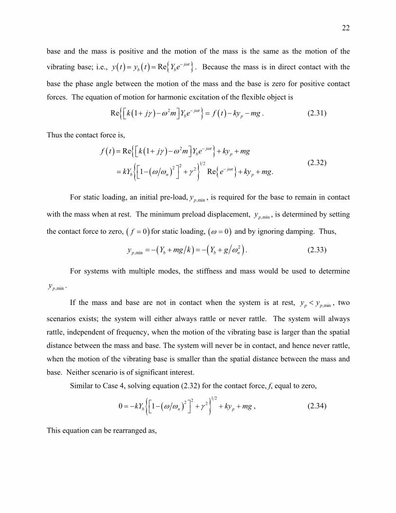
forces. The equation of motion for harmonic excitation of the flexible object is
ω−= = . Because the mass is
( ){ } ( )Re j tpf t ky mgω = − − . (2.31)
Thus the contact force is,
( ) ( ){
21 bk j m Y eγ ω −⎡ ⎤+ −⎣ ⎦
}( ){ } { }
2Re 1 j tf t k j m Y e ky mgωγ ω −⎡ ⎤= + − + +⎣ ⎦ 1 222 21 Re .
b p
j tb n pkY e ky mgωω ω γ −⎡ ⎤= − + + +⎣ ⎦
For static loading, an initial pre-load , is required for the base to remain in contact
ith the mass when at rest. The minimum preload displacement,
the contact force to zero, or static loading,
(2.32)
, ,minpy
w is determined by setting ,minpy ,
( )0f = f ( )0ω = and by ignoring damping. Thus,
( ) ( )2,minp b b ny Y mg k Y g ω= − + + . (2.33)
y .
= −
For systems with multiple modes, the stiffness and mass would be used to determine
If the mass and base are not in contact when the sy
enari
rattle, independent of frequency, when the motion of the vibrating base is larger than the spatial
ce betw
when the motion of the vibrating base is smaller than the spatial distance between the mass and
,minp
stem is at rest, y y< , two ,minp p
sc os exists; the system will either always rattle or never rattle. The system will always
distan een the mass and base. The system will never be in contact, and hence never rattle,
base. Neither scenario is of significant interest.
Similar to Case 4, solving equation (2.32) for the contact force, f, equal to zero,
( ){ }1 222 20 1b n pkY ky mgω ω γ⎡ ⎤= − − + + +⎣ ⎦ , (2.34)
This equation can be rearranged as,
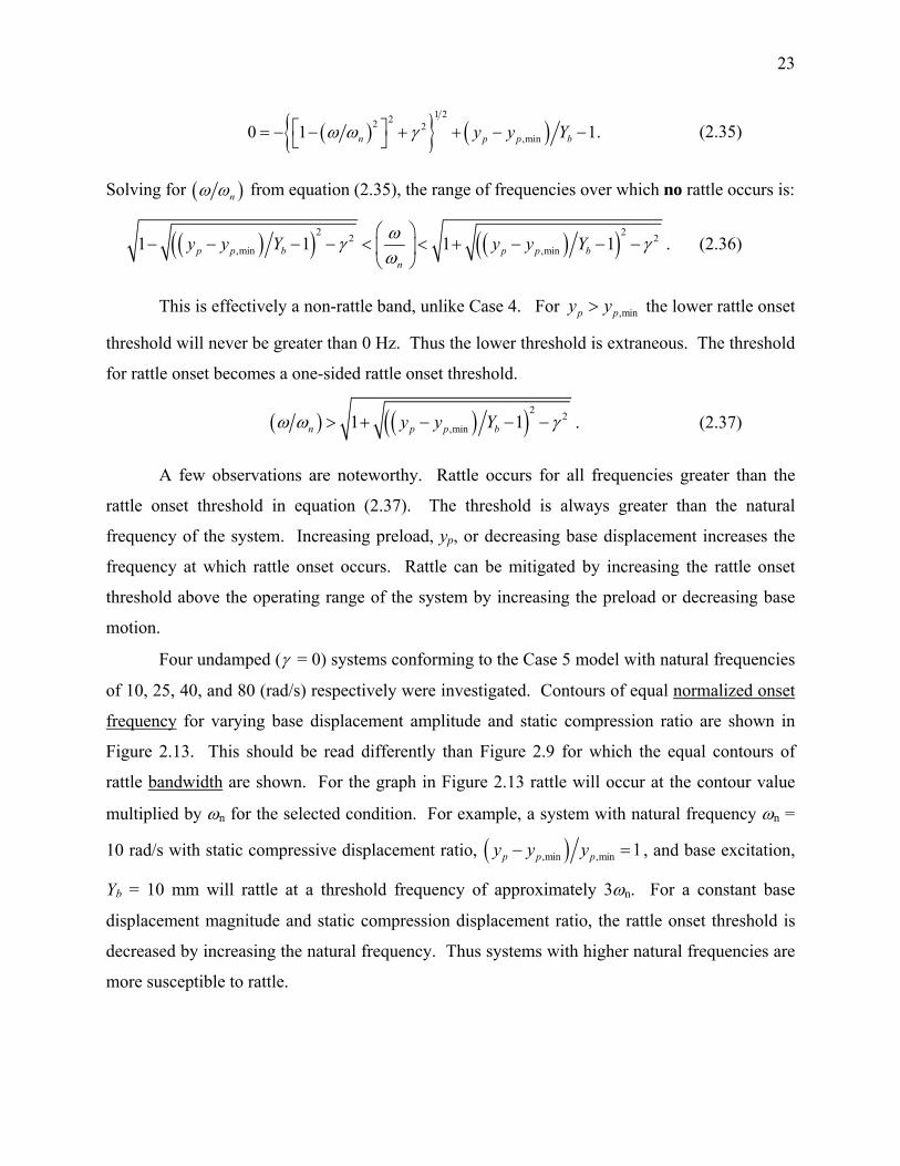
23
( ){ } ( )1 222 2
,min0 1 1.− (2.35) n p p by y Yω ω γ⎡ ⎤= − − + + −⎣ ⎦
Solving for ( )nω ω from equation (2.35), the range of frequencies over which no rattle occurs is:
( )( ) ( )( )2 22 2,min ,min1 1 1p p b p p b
n
y y Y y y Yω 1γ γ− . (2.36) ω
⎛ ⎞− − − − < < + − −⎜ ⎟
⎝ ⎠
s effec
shold will never be greater than 0 Hz. Thus the lower threshold is extraneous. The threshold
r rattle onset becomes a one-sided rattle onset threshold.
This i tively a non-rattle band, unlike Case 4. For y y> the lower rattle onset
thre
,minp p
fo
( ) ( )( )2 2,minn p p b1 1y y Yω ω γ> + − − − . (2.37)
is always greater than the natural
frequency of the system. Increasing preload, yp, or decreasing base displacement increases the
equency at which rattle onset occurs. Rattle can be mitigated
A few observations are noteworthy. Rattle occurs for all frequencies greater than the
rattle onset threshold in equation (2.37). The threshold
fr by increasing the rattle onset
threshold above the operating range of the system by increasing the preload or decreasing base
motion.
Four undamped (γ = 0) systems conforming to the Case 5 model with natural frequencies
of 10, 25, 40, and 80 (rad/s) respectively were investigated. Contours of equal normalized onset
frequency for varying base displacement amplitude and static compression ratio are shown in
Figure 2.13. This should be read differently than Figure 2.9 for which the equal contours of
ttle bra andwidth are shown. For the graph in rattle will occur at the contour value
multiplied by ωn for the selected condition. For example, a system with natural frequency ωn =
10 rad/s with static compressive displacement ratio,
Figure 2.13
( ),min ,min 1p p py y y− = , and base excitation,
Yb = 10 mm will rattle at a threshold frequency of approximately 3ωn. For a constant base
displacement magnitude and static compression displacement ratio, the rattle onset threshold is
decreased by increasing the natural frequency. Thus systems with higher natural frequencies are
more susceptible to rattle.

24
1
1 2
2
3
3
4
4
6
6
88
1010
ωn = 10 γ = 0
Y b (
mm
)
Static Compressive Displacement Ratio(y
p-y
p,min)/y
p,min
Bas
e D
ispl
acem
ent,
0 0.2 0.4 0.6 0.8 10
5
10ωn = 25 γ = 0
m)
1
1
2
2
33
44
668 10
Static Compressive Displacement Ratio(y
p-y
p,min)/y
p,min
Bas
e D
ispl
acem
ent,
Yb (
m
10
5
00 0.2 0.4 0.6 0.8 1
1
1
22 3 3 446
ωn = 40 γ = 0
Static Compressive Displacement Ratio(y
p-y
p,min)/y
p,min
Bas
e D
ispl
acem
ent,
Yb (
mm
)
0 0.2 0.4 0.6 0.8 10
5
10
112 3
ωn = 80 γ = 0
Static Compressive Displacement Ratio(y
p-y
p,min)/y
p,min
Bas
e D
ispl
acem
ent,
Yb (
mm
) 10
0 0.2 0.4 0.6 0.8 10
5
Figure 2.13: Normalized frequency necessary to cause rattle for Case 5 (static compressive displacement ratio vs. base displacement excitation magnitude), γ =0.
As with Case 4, it is important to consider whether damping is important. The same four
systems were investigated using a large structural damping factor, γ = 0.05. The results were
fou ld.
Damping is not an effective mitigation strategy, as with Case 4, unless very high levels of
damping can be introduced. Rattle can be minimized by shifting the rattle onset threshold to
nd to be identical. Thus damping has a negligible effect on the rattle onset thresho
higher frequencies which is achieved by increasing the preload, decreasing the excitation
amplitude, or decreasing the natural frequency of the system. Rattle may be eliminated by
shifting the rattle threshold above the range of frequencies of excitation.

25
2.2.c Case 6: Effects of Preload and Flexible Floor
Case 6 was designed to investigate the influence of both preload (Case 5) and a flexible
floor (Case 4). This model represents a flexible system with applied preload such as a window
system s of this rattle
system were considered, horizontal (without gravity) and vertical (with gravity). The flexible
The static contact force between the masses and the minimum preload is required for
solving the equations of motion for the flexible components in the Case 6 rattle model. For the
ero and damping effects are insignificant.
The schematic and free body diagram for the static case of Case 6 is shown in Figure 2.14 and
with a gasket or a door in a door frame with a gasket. Two orientation
surface was modeled as having mass, m1, with complex stiffness, k1(1+jγ1), where γ1 is the
structural damping coefficient. The flexible rattle object, which is preloaded, was modeled as
having mass, m2 with complex stiffness, k2(1+jγ2), where γ2 is the structural damping coefficient.
When the object, m2, and the flexible floor, m1, move together with the same velocity, there is no
rattle.
2.2.c.i Case 6: Static Force and Minimum Preload
static case, the velocity of the flexible components is z
Figure 2.15, respectively. The effect of preload was included by enforcing the static
displacement, yp. The system was initially compressed from equilibrium by a static compressive
displacement, yp.
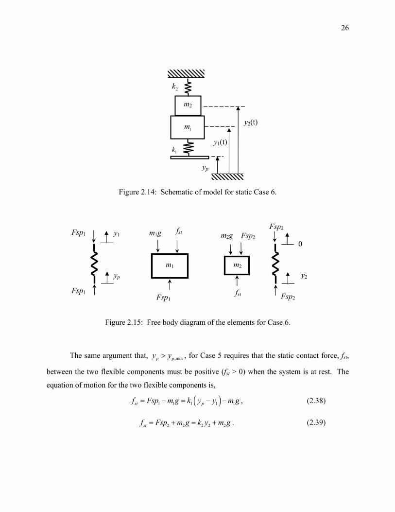
26
Figure 2.14: Schematic of model for static Case 6.
Figure 2.15: Free body diagram of the elements for Case 6.
The same argument that, , for Case 5 requires that the static contact force, fst,
between the two flexible components must be positive (fst > 0) when the system is at rest. The
equation of motion for the two flexible components is,
,minp py y>
( )1 1 1 1 1st pf Fsp m g k y y m g= − = − − , (2.38)
2 2 2 2 2stf Fsp m g k y m g= + = + . (2.39)
m2
2k
1m
1k
y2(t)
y1(t)
yp
m2g
m2
Fsp2 fst
fst
m1g
Fsp1
m1
Fsp2
Fsp2 y1
yp
Fsp1
Fsp1
0
y2

27
The assumption that the masses are in contact when the system is at rest (fst > 0), results in the
following constraint equation:
1 2y y y= = . (2.40)
By multiplying equation (2.38) by k2 and equation (2.39) by k1 then substituting the constraint
equation (2.40) in for y, the static force is
( ) ( )1 2 1 2 1 2 2 1st pk k f k k y k m k m g+ = + − . (2.41)
The natural frequency of the total system is n K Mω = , where 1 2K k k= + ,
1 2M m m= + , the natural frequency of the lower flexible component is 1 1k mω = 1 , and the
natural frequency of the upper flexible component is 2 2k mω = 2 . The system is initially
compressed from equilibrium by the static displacement, yp.
The contact force, ,st vertf , at the static equilibrium for a vertical system is:
( )
( ) ( )
1 2 1 2 2 1,
1 2
2 21 2 2 11 1
pst vert
p
k k y k m k m gf
k k
k k K y gω ω
+ −=
+
.⎡ ⎤= + −⎣ ⎦
(2.42)
The minimum amount of preload for which the flexible systems will remain in contact when the
system is at rest is, yp,min. The minimum preload, yp,min, is determined by setting equation (2.42)
to zero and solving for yp. Thus, ( )2 2,min 1 21 1py gω ω= − . Therefore equation (2.42) simplifies
to
( )( ), 1 2 ,mst vert p pf k k K y y= − in . (2.43)
For a horizontal system, the contact force, ,st horzf , at static equilibrium is:
1 2,st horz p
k kf yK
= . (2.44)
For the horizontal orientation yp,min = 0.
28
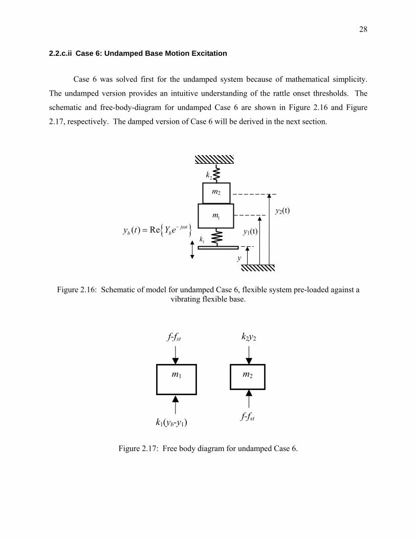
2.2.c.ii Case 6: Undamped Base Motion Excitation
Case 6 was solved first for the undamped system because of mathematical simplicity.
The undamped version provides an intuitive understanding of the rattle onset thresholds. The
schematic and free-body-diagram for undamped Case 6 are shown in Figure 2.16 and Figure
2.17, respectively. The damped version of Case 6 will be derived in the next section.
Figure 2.16: Schematic of model for undamped Case 6, flexible system pre-loaded against a vibrating flexible base.
Figure 2.17: Free body diagram for undamped Case 6.
m2
2k
1m
1k
y2(t)
{ }( ) Re j tb by t Y e ω−= y1(t)
y
k2y2f-fst
m1 m2
f-fst k1(yb-y1)

29
By using Newton’s 2nd law of motion, the equations of motion were expressed as,
1 1 1 1 1 bm y k y k y f fst+ = − + , (2.45)
2 2 2 2 stm y k y f f+ = − , (2.46)
where yb is the base excitation, f is the contact force between the flexible components, and fst is
the static contact force in the system. For the case when rattle does not occur, the masses move
together with the same motion (i.e., y1 = y2) and the contact force is positive. The motion of the
masses moving together, M, is described in complex notation using, ( ) { }Re j ty t Y e ω−= and
( ) { }2 Re j ty t Y e ωω −= − . The motion of the vibrating base is described by ( ) { }Re j tb by t Y e ω−= .
For motion when rattle does not occur, the masses move together with the same displacement
and the contact force is positive. The solution for the case where ( 1 2i.e., Y Y Y= = ) 1 2y y y= = ,
is obtained from equations (2.45) and (2.46):
( )
{12( ) Re
1}j tb
n
k Y Ky t e ω
ω ω−=
−. (2.47)
Substituting equation (2.47) into (2.46) and solving for the contact force yield,
( ) ( )( )
{ }2
21 22
1Re
1j tb
stn
k k Yf tK
ωω ω
ω ω−−⎛ ⎞= ⎜ ⎟
⎝ ⎠ −e f+ , (2.48)
where fst is the static contact force. The first term on the right hand side of (2.48) is the dynamic
contact force.
The spring is initially compressed from equilibrium by a displacement yp. The
requirement that ensures that the system is in contact with the base when the system
is at rest. Rattle onset occurs when the contact force becomes zero (f = 0), which is assumed to
occur at peak acceleration amplitudes when
,minp py y>
1j te ω = − . The rattle band for the vertical system is
solved in terms of ( n )ω ω from equation (2.48) and (2.42):
For 1 n 2ω ω ω> > where system 1 is either stiffer or has less mass than system 2:
( ) ( )
,min ,min2 2
,min 2 ,min 2
p p b p p b
np p n b p p n b
y y Y y y Y
y y Y y yωωω ω ω ω
− + − −⎛ ⎞< <⎜ ⎟
− + − −⎝ ⎠ Y. (2.49)

30
For 1 n 2ω ω ω< < where system 1 is more flexible or has more mass than system 2:
( ) ( ),min ,min
2 2,min 2 ,min 2
p p b p p b
np p n b p p n b
y y Y y y Y
y y Y y yωωω ω ω ω
− − − +⎛ ⎞< <⎜ ⎟
− − − +⎝ ⎠ Y. (2.50)
2.2.c.iii Case 6: Damped Base Motion Excitation
Case 6 with damping was investigated to account for structurally dissipative elements.
The schematic and free body diagram for the damped Case 6 are shown in Figure 2.18 and
Figure 2.19, respectively.
Figure 2.18: Schematic of model for damped Case 6, flexible system pre-loaded against a vibrating flexible base.
m2
( )2 21k jγ+
m1 y2(t)
( )1 11k j y1(t) γ+
( ) { }Re j tb by t Y e ω−=
yp

31
f-fst k2y2(1+jγ2)
m1 m2
f-fst k1(yb-y1)(1+jγ1)
Figure 2.19: Free body diagram for Case 6, including damping.
The equations of motion for harmonic excitation of Case 6 with damping is,
( ){ } ( ){ }21 1 1 1 1 1Re 1 Re 1j t j t
bk j m Y e k j Y e fωγ ω γ− −⎡ ⎤+ − + = + − +⎣ ⎦ stfω , (2.51)
( ){ }22 2 2 2Re 1 j t
stk j m Y e fωγ ω −⎡ ⎤+ − + = −⎣ ⎦ f . (2.52)
Following the same approach as for previous cases.
( ) ( )21 1 2 2 1 11bK j k k M Y k Y jγ γ ω γ⎡ ⎤+ + − = +⎣ ⎦ , (2.53)
Therefore,
( ) ( )( )
( ) ( )
1 12
1 1 2 2
1 2
21 1
2 221 1 2 2
1
1 .1
b
jb
n
k Y jY j
K M j k k
k Y eK k k K
φ
γω
ω γ γ
γ
ω ω γ γ
−
+=
⎡ ⎤− + +⎣ ⎦
⎧ ⎫+⎪ ⎪⎛ ⎞= ⎨ ⎬⎜ ⎟
⎝ ⎠ ⎡ ⎤⎪ ⎪⎡ ⎤− + +⎣ ⎦⎣ ⎦⎩ ⎭
(2.54)
Substituting equation (2.54) into (2.52) and solving for the total contact force, f, yields,
( )( ) ( )
( ) ( )( ){
1 2222 21 2 2
1 22 22
1 1 2 2
1 1Re
1
j tst b
n
k kf t f Y eK k k K
ω φγ ω ω γ
ω ω γ γ
− +
⎧ ⎫⎡ ⎤⎡ ⎤+ − +⎪ ⎪⎢ ⎥⎣ ⎦⎪ ⎪⎛ ⎞ ⎣ ⎦= + ⎨ ⎬⎜ ⎟⎝ ⎠ ⎡ ⎤⎪ ⎪⎡ ⎤− + +⎣ ⎦⎣ ⎦⎪ ⎪⎩ ⎭
} . (2.55)

32
The spring is initially compressed from equilibrium by displacement yp and is introduced
through the static contact force, fst, term. As discussed in the previous section it is required that
. This ensures that the system is in contact with the base when the system is at rest.
Rattle onset occurs when the contact force becomes zero
,minp py y>
( )0f = , which is assumed to occur at
peak acceleration amplitudes when ( ) 1j te ω φ− + = − . Solving for rattle onset for the vertical
orientation by substituting equation (2.43) for the static contact force,
( )( ) ( )
( ) ( )
1 2222 21 2 2
1 2 1 2,min 2 22
1 1 2 2
1 10
1p p b
n
k k k ky y YK K k k K
γ ω ω γ
ω ω γ γ
⎧ ⎫⎡ ⎤⎡ ⎤+ − +⎪ ⎪⎢ ⎥⎣ ⎦⎪ ⎪⎛ ⎞ ⎛ ⎞ ⎣= − − ⎦⎨ ⎬⎜ ⎟ ⎜ ⎟
⎝ ⎠ ⎝ ⎠ ⎡ ⎤⎪ ⎪⎡ ⎤− + +⎣ ⎦⎣ ⎦⎪ ⎪⎩ ⎭
, (2.56)
this can be rearranged as:
( ) ( ) ( ) ( )2
2 222 22 21 1 2 2 1 2 2
,min
0 1 1 1bn
p p
Yk k Ky y
ω ω γ γ γ ω ω⎛ ⎞
γ⎡ ⎤⎡ ⎤ ⎡ ⎤⎡ ⎤= − + + + + − +⎜ ⎟⎣ ⎦ ⎢ ⎥⎜ ⎟⎣ ⎦ ⎣ ⎦− ⎣ ⎦⎝ ⎠.(2.57)
By rearranging equation (2.57) in the following manner, where ( )2nμ ω ω=
2 0,A B Cμ μ+ + = (2.58)
where,
(24
21
2 ,min
1 n b
p p
YAy y
ω γω
⎡ ⎤⎛ ⎞⎛ ⎞⎢= + +⎜ ⎟⎜ ⎟ ⎜ ⎟−⎢ ⎥⎝ ⎠ ⎝ ⎠⎣ ⎦)1 ⎥ (2.59)
(22
21
2 ,min
2 1 1n b
p p
YBy y
ω γω
⎡ ⎤⎛ ⎞⎛ ⎞⎢= − + +⎜ ⎟⎜ ⎟ ⎜ ⎟−⎢ ⎥⎝ ⎠ ⎝ ⎠⎣ ⎦)⎥ (2.60)
( )(22
2 21 1 2 21 2
,min
1 b
p p
Yk kCK y y
γ γ γ γ⎡ ⎤⎛ ⎞+⎛ ⎞⎢ ⎥= + + + +⎜ ⎟⎜ ⎟ ⎜ ⎟−⎢ ⎥⎝ ⎠ ⎝ ⎠⎣ ⎦
)1 1 (2.61)
The solution to the quadratic equation for equation (2.58) for the rattle onset threshold for
normalized frequency is,

33
2 2
1,24
2n
B B ACA
ω μω
⎛ ⎞ − ± −= =⎜ ⎟
⎝ ⎠. (2.62)
Thus the upper and lower rattle onset thresholds are,
2
,
42n U L
B B ACA
ωω
± −⎛ ⎞=⎜ ⎟
⎝ ⎠
L U
, (2.63)
such that ω ω< and the lower rattle threshold, ωL, must be greater than 0 Hz. The rattle band
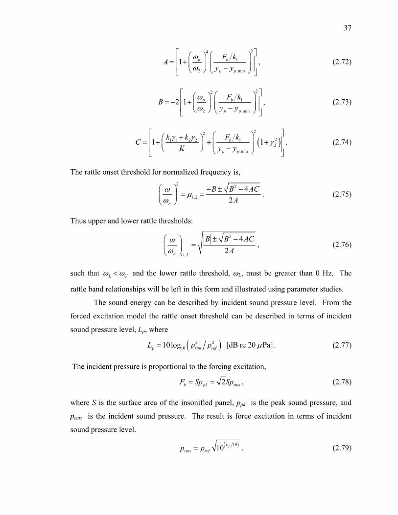
relationships will be left in this form and illustrated using parameter studies.
In Figure 2.20, the contours of rattle bandwidth, λ, are shown for various ratios of natural
frequencies, ( )1 2Rω ω ω= , where the natural frequency of the lower flexible component is
1 1 1k mω = , and the natural frequency of the upper flexible component is 2 2 2k mω = . The
ratio, ( )1 2Rω ω ω=
1 2
, decreases across and down the subplot rows. Each of the eight systems are
evaluated with no damping, (γ1 = γ2 = 0). Several general observations may be made from Figure
2.20. By increasing the preload the rattle band is reduced for constant excitation. As the ratio of
component natural frequencies, ωR, approaches unity the rattle bandwidth, λ, approaches unity.
When ωR = 1 rattle onset occurs for all preload and excitation amplitudes. For ω ω
1 2
and also
ω ω
1 2 n
rattle bandwidth is decreased for constant preload and excitation amplitude.
From these observations several rattle mitigation strategies are evident. Increasing
preload decreases the rattle band. In practical systems it is unlikely that ω ω ω= =
1 2
exactly.
However, for flexible components of similar stiffness and mass,
ω ω→ . Thus the effect of
preload is diminished and rattle onset occurs for all preload and excitation amplitudes. Thus, the
mitigation strategy is to either stiffen or soften one of the flexible components involved in the
rattle system to reduce the rattle band. As with Case 5, damping was found to be negligible.

34
0.25
0.50.75
1
ω1/ω2 = 1.8
Preload Ratio( yp - yp,min ) / yp,min
Base
Disp
lace
men
t Exc
itatio
n, Y
b (m
)
0 0.1 0.20
0.2
0.4
0.6
0.8
1
0.25
0.5
0.751
ω1/ω2 = 1.5
Preload Ratio( yp - yp,min ) / yp,min
Base
Disp
lace
men
t Exc
itatio
n, Y
b (m
)0 0.1 0.2
0
0.2
0.4
0.6
0.8
1
0.250.5
0.75
11.25
ω1/ω2 = 1.25
Preload Ratio( yp - yp,min ) / yp,min
Base
Disp
lace
men
t Exc
itatio
n, Y
b (m
)
0 0.1 0.20
0.2
0.4
0.6
0.8
1
0.250.50.751 1.251.5
ω1/ω2 = 0.99
Preload Ratio( yp - yp,min ) / yp,min
Base
Disp
lace
men
t Exc
itatio
n, Y
b (m
)
0 0.1 0.20
0.2
0.4
0.6
0.8
1
0.250.50.75
11.251.5
ω1/ω2 = 0.9
Preload Ratio( yp - yp,min ) / yp,min
Base
Disp
lace
men
t Exc
itatio
n, Y
b (m
)
0 0.1 0.20
0.2
0.4
0.6
0.8
1
0.25
0.5
0.75
11.251.5
ω1/ω2 = 0.8
Preload Ratio( yp - yp,min ) / yp,min
Base
Disp
lace
men
t Exc
itatio
n, Y
b (m
)
0 0.1 0.20
0.2
0.4
0.6
0.8
1
0.25
0.50.75
11.25
1.51.75
ω1/ω2 = 0.7
Preload Ratio( yp - yp,min ) / yp,min
Base
Disp
lace
men
t Exc
itatio
n, Y
b (m
)
0 0.1 0.20
0.2
0.4
0.6
0.8
1
0.25
0.50.75
11.251.5
1.75
ω1/ω2 = 0.6
Preload Ratio( yp - yp,min ) / yp,min
Base
Disp
lace
men
t Exc
itatio
n, Y
b (m
)
0 0.1 0.20
0.2
0.4
0.6
0.8
1
34
Figure 2.20: Contours of equal non-dimensional rattle bandwidth, λ, for Case 6 (static compressive displacement vs. base displacement excitation magnitude), γ1=γ2 = 0.

35
2.2.c.iv Forced excitation
The next case study is for the same system excited with harmonic forced
excitation, where Fb is the force magnitude. This is a case study of a situation where the
flexible floor is excited directly by a force. In the application to airport noise, this may
be a simple model for a wall excited by sound energy, with a preloaded object resting
against it. The schematic model and free body diagram is shown in Figure 2.21 and
Figure 2.19, respectively.
m1
m2
( )1 11k jγ+
y1(t)
y2(t)
yp
( )2 21k jγ+
( ) { }Re j tb bf t F e ω−=
Figure 2.21: Schematic of model for Case 6, flexible system pre-loaded against a vibrating flexible base.
The development for the forced system is similar to the motion excitation system.
The equations of motion for force excitation of Case 6 with damping is,
( ){ } { } ( )21 1 1 1Re 1 Rej t j t
bk j m Y e F e f tω ωγ ω − −⎡ ⎤+ − = − +⎣ ⎦ stf , (2.64)
( ){ } ( )22 2 2 2Re 1 j t
stk j m Y e f tωγ ω −⎡ ⎤ f+ − + = −⎣ ⎦ . (2.65)
The solution for bulk motion, where 1 2y y y= = , is obtained by adding equations
(2.64) and (2.65).
( ) 21 1 2 2 bK j k k M Y Fγ γ ω⎡ ⎤+ + − =⎣ ⎦ . (2.66)

36
Therefore,
( )( )
( ) ( )
21 1 2 2
1 2
2 221 1 2 2
,
1 .1
b
jb
n
FY jK M j k k
F eK k k K
φ
ωω γ γ
ω ω γ γ
−
=⎡ ⎤− + +⎣ ⎦
⎧ ⎫⎪ ⎪⎛ ⎞= ⎨ ⎬⎜ ⎟
⎝ ⎠ ⎡ ⎤⎪ ⎪− + +⎡ ⎤⎣ ⎦⎣ ⎦⎩ ⎭
(2.67)
Substitution of equation (2.67) into (2.65) and solving for the contact force, f, yields
( )( )
( ) ( )( ){
1 222 22 22
2 221 1 2 2
1Re
1
j tbst
n
k Ff t f eK k k K
ω φω ω γ
ω ω γ γ
− +
⎧ ⎫⎡ ⎤− +⎪ ⎪⎛ ⎞ ⎣ ⎦= + ⎨ ⎬⎜ ⎟⎝ ⎠ ⎡ ⎤⎪ ⎪− + +⎡ ⎤⎣ ⎦⎣ ⎦⎩ ⎭
}
)
. (2.68)
The spring is initially compressed from equilibrium by displacement yp and is
introduced through the static contact force, fst, term along with gravitational loads. As
discussed in the previous section it is required that . This ensures that the
system is in contact with the base when the system is at rest.
,minp py y>
Rattle onset will occur when the contact force becomes zero ( , which
occurs at peak acceleration amplitudes when
0f =
( ) 1j te ω φ− + = − . Solving for rattle onset for
the vertical orientation by substituting equation (2.43) for the static contact force,
( )( )
( ) ( )
1 222 22 2
1 2 2,min 2 22
1 1 2 2
10
1p p b
n
k k ky y FK K k k K
ω ω γ
ω ω γ γ
⎧ ⎫⎡ ⎤⎡ ⎤− +⎪ ⎪⎢ ⎥⎣ ⎦⎪ ⎪⎛ ⎞ ⎛ ⎞ ⎣ ⎦= − − ⎨ ⎬⎜ ⎟ ⎜ ⎟⎝ ⎠ ⎝ ⎠ ⎡ ⎤⎪ ⎪⎡ ⎤− + +⎣ ⎦⎣ ⎦⎪ ⎪⎩ ⎭
, (2.69)
this can be rearranged as:
( ) ( ) ( )2
2 222 2 211 1 2 2 2 2
,min
0 1 1bn
p p
F kk k Ky y
ω ω γ γ ω ω⎛ ⎞
γ⎡ ⎤⎡ ⎤ ⎡ ⎤⎡ ⎤= − + + + − +⎜ ⎟⎣ ⎦ ⎢ ⎥⎜ ⎟⎣ ⎦ ⎣ ⎦− ⎣ ⎦⎝ ⎠.(2.70)
Rearranging in the following manner, where ( )2nμ ω ω= ,
2 0A B Cμ μ+ + = , (2.71)
where,
37
24
1
2 ,mi
1 n b
p p
F kAy y
ωω n
⎡ ⎤⎛ ⎞⎛ ⎞⎢ ⎥= + ⎜⎜ ⎟ ⎜ −⎟⎟⎢ ⎥⎝ ⎠ ⎝ ⎠⎣ ⎦
, (2.72)
22
1
2 ,mi
2 1 n b
p p
F kBy y
ωω n
⎡ ⎤⎛ ⎞⎛ ⎞⎢ ⎥= − + ⎜⎜ ⎟ ⎜ −⎟⎟⎢ ⎥⎝ ⎠ ⎝ ⎠⎣ ⎦
, (2.73)
(22
211 1 2 22
,min
1 b
p p
F kk kCK y y
γ γ γ⎡ ⎤⎛ ⎞+⎛ ⎞⎢ ⎥= + + +⎜ ⎟⎜ ⎟ ⎜ ⎟−⎢ ⎥⎝ ⎠ ⎝ ⎠⎣ ⎦
)1 . (2.74)
The rattle onset threshold for normalized frequency is,
2 2
1,24
2n
B B ACA
ω μω
⎛ ⎞ − ± −= =⎜ ⎟
⎝ ⎠. (2.75)
Thus upper and lower rattle thresholds:
2
,
42n U L
B B ACA
ωω
± −⎛ ⎞=⎜ ⎟
⎝ ⎠, (2.76)
such that L Uω ω< and the lower rattle threshold, ωL, must be greater than 0 Hz. The
rattle band relationships will be left in this form and illustrated using parameter studies.
The sound energy can be described by incident sound pressure level. From the
forced excitation model the rattle onset threshold can be described in terms of incident
sound pressure level, Lp, where
( )2 21010log [dB re 20 Pa]p rms refL p p μ= . (2.77)
The incident pressure is proportional to the forcing excitation,
2b pk rF Sp Sp= = ms , (2.78)
where S is the surface area of the insonified panel, ppk is the peak sound pressure, and
prms is the incident sound pressure. The result is force excitation in terms of incident
sound pressure level.
( )1010 pLrms refp p= . (2.79)

38
By substitution of equation (2.78) into (2.79) the following is obtained
( )102 10 pLb refF Sp= . (2.80)
In Figure 2.22 the contours of rattle bandwidth, λ, are shown for various ratios of
natural frequencies, ( )1 2Rω ω ω= for the incident pressure excitation system. The ratio,
( )1 2Rω ω ω= , decreases across and down the subplot rows. Each of the eight systems
are evaluated with no damping, γ1=γ2 = 0. Similar observations are made as for Figure
2.20. Increasing preload decreases the rattle bandwidth. Dissimilar natural frequencies
of the components also decrease the rattle bandwidth for constant preload and incident
sound pressure level. A plot of the forced system with damping is not included because
the effect of damping is negligible, as with Case 5.

39
0.25
.575
1
ω1/ω2 = 1.95
Preload Ratio( yp - yp,min ) / yp,min
Inci
dent
Sou
nd P
ress
ure
Leve
l, L
p (d
B re
20 μ
Pa)
0 0.1 0.230
40
50
60
70
80
90
100
110
0.25
0.5
75
1
ω1/ω2 = 1.5
Preload Ratio( yp - yp,min ) / yp,min
Inci
dent
Sou
nd P
ress
ure
Leve
l, L
p (d
B re
20 μ
Pa)
0 0.1 0.230
40
50
60
70
80
90
100
110
0.250.5
0.7511.25
ω1/ω2 = 1.25
Preload Ratio( yp - yp,min ) / yp,min
Inci
dent
Sou
nd P
ress
ure
Leve
l, L
p (d
B re
20 μ
Pa)
0 0.1 0.230
40
50
60
70
80
90
100
110
0.250.5
0.7511.25
1.5
ω1/ω2 = 0.99
Preload Ratio( yp - yp,min ) / yp,min
Inci
dent
Sou
nd P
ress
ure
Leve
l, L
p (d
B re
20 μ
Pa)
0 0.1 0.230
40
50
60
70
80
90
100
110
0.250.5
0.7511.251.5
ω1/ω2 = 0.8
Preload Ratio( yp - yp,min ) / yp,min
Inci
dent
Sou
nd P
ress
ure
Leve
l, L
p (d
B re
20 μ
Pa)
0 0.1 0.230
40
50
60
70
80
90
100
110
0.25
.575
11.25
1.5
1.75
ω1/ω2 = 0.5
Preload Ratio( yp - yp,min ) / yp,min
Inci
dent
Sou
nd P
ress
ure
Leve
l, L
p (d
B re
20 μ
Pa)
0 0.1 0.230
40
50
60
70
80
90
100
110
0.25
0.50.7511.25
1.51.75
2
ω1/ω2 = 0.1
Preload Ratio( yp - yp,min ) / yp,min
Inci
dent
Sou
nd P
ress
ure
Leve
l, L
p (d
B re
20 μ
Pa)
0 0.1 0.230
40
50
60
70
80
90
100
110
0.250.5
751
1.251.5
752
ω1/ω2 = 0.01
Preload Ratio( yp - yp,min ) / yp,min
Inci
dent
Sou
nd P
ress
ure
Leve
l, L
p (d
B re
20 μ
Pa)
0 0.1 0.230
40
50
60
70
80
90
100
110
Figure 2.22: Contours of equal non-dimensional rattle bandwidth, λ, for Case 6 (static compressive displacement vs. incident sound pressure level), γ1=γ2 = 0.
39
40
3 EXPERIMENTAL RATTLE STUDY A rattle experiment was conducted at Purdue University’s Ray W. Herrick Laboratories
in order to evaluate the principles identified in the analytical rattle models. Four windows
known to be susceptible to rattle were excited via high-fidelity playback of three, high-
amplitude, low-frequency noise signals. The signals included pre-recorded aircraft take-off
noise, a swept sine signal, and pink noise. The vibration and acoustic response of each of the
windows was measured to determine the relationship between frequency and acceleration
amplitude that is required for rattle onset.
3.1 Objective
The objective of the experiment was to identify the onset of rattle by investigating the
response of window panels insonified with large amplitude, low-frequency sound waves.
3.2 Test Method
Four windows that were known to rattle were selected. The dynamic response of the four
windows was measured first. The mode shapes of the windows were found to correspond to the
low order modes of a large panel as expected. For rattle evaluation, the four windows were
insonified at four different amplitudes using three input signal recordings. The recordings
included aircraft take-off, swept sine, and pink noise. Each signal was played through an Altec
1201A loudspeaker and BagEnd P-D18E-R subwoofer configuration capable of radiating flat-
spectrum noise from 20 Hz to 15 kHz. The excitation source is shown in Figure 3.1.

41
Figure 3.1: Loudspeaker set-up for rattle experiment.
For each signal, a series of four amplitudes were selected such that the lowest amplitude
did not produce rattle for any of the four windows while the highest two signal strengths caused
audible rattle of the window. Response of each window was measured using two accelerometers
placed on the windows away from the primary nodal lines of the modes of the windows. Sound
pressures inside and outside of the test room were also measured.
Figure 3.2: Experimental set-up at Herrick Labs, Loudspeakers directed at set of two large and two small windows.

42
Figure 3.3: Experimental set-up at Herrick Labs, Close-up of four windows.
The placement of loudspeakers and microphones relative to the panels (windows) was
set-up as specified by ASTM E-966 [9], ISO 140-5 [10] and ISO 140-14 [11] standards. In
Figure 3.2 the loudspeakers are shown directed at the bank of windows on the left, including two
large (upper) windows and two small (lower) windows. The floor-to-ceiling windows shown in
the center of Figure 3.2 were not measured in this study. A close up of the four windows is
shown in Figure 3.3 with accelerometers attached to each window and microphones placed to
record sound indoors and outdoors of the room. A schematic of the loudspeaker and microphone
placements is shown in Figure 3.4.
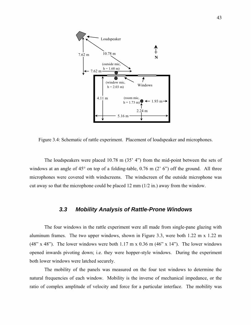
43
1.93 m
5.16 m
7.62 m
4.11 m
2.24 m
Loudspeaker
Windows
(room mic, h = 1.73 m)
10.78 m
(outside mic, h = 1.68 m)
(window mic, h = 2.03 m)
N
7.62 m
Figure 3.4: Schematic of rattle experiment. Placement of loudspeaker and microphones.
The loudspeakers were placed 10.78 m (35’ 4”) from the mid-point between the sets of
windows at an angle of 45° on top of a folding-table, 0.76 m (2’ 6”) off the ground. All three
microphones were covered with windscreens. The windscreen of the outside microphone was
cut away so that the microphone could be placed 12 mm (1/2 in.) away from the window.
3.3 Mobility Analysis of Rattle-Prone Windows
The four windows in the rattle experiment were all made from single-pane glazing with
aluminum frames. The two upper windows, shown in Figure 3.3, were both 1.22 m x 1.22 m
(48” x 48”). The lower windows were both 1.17 m x 0.36 m (46” x 14”). The lower windows
opened inwards pivoting down; i.e. they were hopper-style windows. During the experiment
both lower windows were latched securely.
The mobility of the panels was measured on the four test windows to determine the
natural frequencies of each window. Mobility is the inverse of mechanical impedance, or the
ratio of complex amplitude of velocity and force for a particular interface. The mobility was

44
measured by striking each window with an impact hammer and measuring the vibration response
with an accelerometer. For post-process analysis, a force window with 10% trigger was applied
to the input channel (PCB Type 086C03 medium impact hammer) and an exponential window
with time constant, τ = 1.3896 seconds, to the output channels (PCB Type 333B32
accelerometers) to minimize the effects of background noise.
In order to accurately identify higher-order mode shapes, five accelerometers were placed
asymmetrically on the upper windows away from nodal lines as shown in Figure 3.5. Four
accelerometers were mounted on the lower windows as shown in Figure 3.6. The impact
hammer was struck at each of the grid points and the drive-point and cross mobilities were
measured using the accelerometers. Multiple Reference Impact Testing (MRIT) and X-Modal
software [12], written at the University of Cincinnati and implemented by the Purdue University
structural-health-monitoring group, was used to capture mobility data and identify natural
frequencies of the windows. MRIT was used to capture data, while X-Modal was used to
identify natural frequencies from a synthesis of the response for all grid-point impact excitations.
1 2 3 4 5 6 7
8 9 10 11 12 13 14
15 16 17 18 19 20 21
22 23 24 25 26 27 28
29 30 31 32 33 34 35
36 37 38 39 40 41 42
43 44 45 46 47 48 49
1.22 m0.2 m
0.2 m
1.22 m
Figure 3.5: Grid-point locations for 1.22 m x 1.22 m (48” x 48”) upper window with five accelerometer locations denoted by black dots.

45
1 2 3 4 5
106 7 8 911 12 13 14 1516 17 18 19 20
21 22 23 24 25
1168
390
974
178119
23
35
548
Figure 3.6: Grid-point locations for 1.17 m x 0.36 m (46” x 14”) lower window with four accelerometer locations denoted by black dots. Dimensions in mm.
The natural frequencies of the four windows are shown in Table 3.1. The natural
frequencies are similar for the windows having the same geometry, as expected. Differences can
be attributed to the age of windows and irregularities at the window frame boundary conditions.
Table 3.1: Natural frequencies of four rattle-prone windows.
Lower East
Lower West
Upper East
Upper West
30 37 26 2535 52 43 4144 68 53 5151 91 70 6665 122 90 87
121 97 91160 106 126
134 133137 145154 158172 165181 173221 203242 239263 252267 262
Natural Freqencies (Hz)
46
3.4 Experimental Results
The response of one window (lower east), in the bottom left corner of Figure 3.3, to the
highest signal strength swept sine, aircraft take-off, and pink noise signals is presented in this
section. The complete results for all four windows are compiled in the Appendices.
Spectrogram plots are contained in Appendix A and acceleration level versus frequency for all
four windows is contained in Appendix B.
Measurement locations include an outdoor microphone, which is used to measure the
noise source, an indoor room microphone, and window-mounted accelerometers. All vibration
response plots are the response measured using the accelerometer at location 33 as shown in
Figure 3.5 for the upper window and location 19 as shown in Figure 3.6 for the lower
windowsFigure .
The background noise measured using the outside microphone is shown in Figure 3.7 in
the form of a spectrogram. The background noise spectrogram is shown in the top subplot. To
create the spectrogram an FFT length of 4096 samples was included per time slice with a
Hanning window applied and 85% overlap. The sampling frequency was 4096 Hz. The time
history of the (1/8) second time-averaged equivalent level, Leq, is shown in the bottom subplot of
the respective figures. Unweighted, A-weighted, and C-weighted equivalent sound levels are
shown in the lower subplot. The vibration response of the lower east window to the background
noise is shown in Figure 3.8.
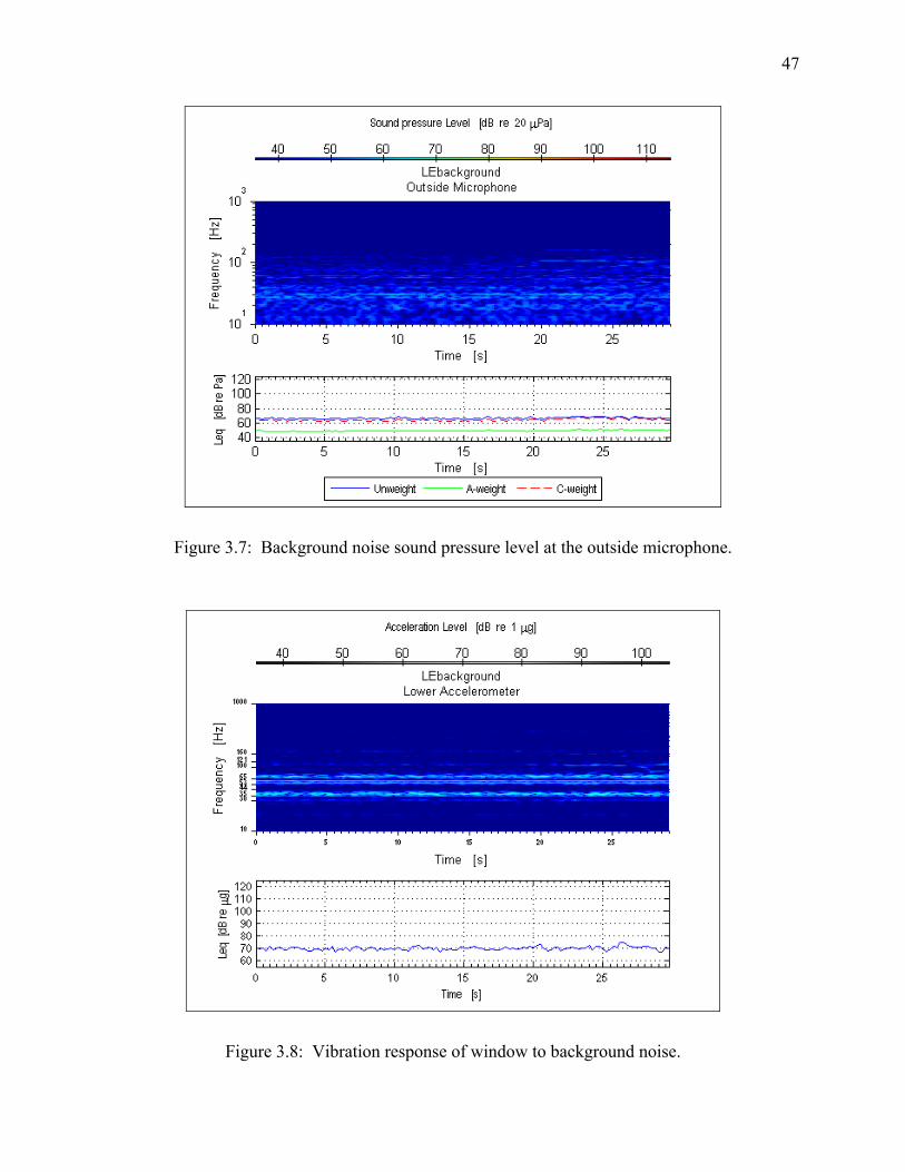
47
Figure 3.7: Background noise sound pressure level at the outside microphone.
Figure 3.8: Vibration response of window to background noise.

48
The horizontal highlights of the window vibration response spectrogram shown in Figure
3.8 correspond to the low order natural frequencies of the window. The dotted line at 100 dB on
the Leq subplot represents a rattle threshold determined by this experimental study which will be
discussed later. For now it is noteworthy to mention that the response of the window is well
below the experimental rattle threshold despite larger acceleration response at the natural
frequencies.
3.4.a Swept Sine Excitation
For the highest signal strength for the swept sine signal, the resulting overall sound
pressure level at the outside window surface was 100 dBC as shown in Figure 3.9. The
acceleration response of the lower east window to the highest amplitude swept sine signal is
shown in Figure 3.10. The swept sine signal sweeps down from 700 Hz to 20 Hz, repeating after
78 seconds. The bottom-most diagonal line shown in both figures is the response to the input
frequency from the swept sine frequency generator. The parallel lines are due to harmonic
distortion caused by driving the loudspeakers at high amplitudes: i.e. beyond their linear range.
The microphone and accelerometer responses were recorded simultaneously.

49
Figure 3.9: Sound pressure level measured at the outside microphone to the swept sine.
Figure 3.10: Vibration response of the lower left window to highest swept sine signal amplitude with overall sound pressure level of 100 dBC.

50
Rattle events occurred at the frequencies of the vertical highlights, indicating non-linear,
broadband window response to acoustical excitation. Previous studies also described rattle as a
broadband response [13]. The rattle onset typically occurred when the acceleration level
exceeded 100 dB re 1 μg or 0.1 grms. In the frequency range shown (10-1000 Hz) in Figure 3.9
rattle is not “heard” by the outside microphone. The spectrogram in Figure 3.11 is identical to
Figure 3.10 except the frequency scale is over the low frequency range (10-200 Hz).
Figure 3.11: Same plot as Figure 3.10 but with smaller frequency scale (10-200 Hz).
The bottom-most diagonal line is the swept sine (700-20 Hz) from the function generator
and again the parallel lines are harmonic distortion from driving the loudspeaker at high
amplitudes. The tick marks on the frequency axis indicate the resonances of the window which
were determined by the mobility test described earlier. The first rattle event (seen as a vertical
highlight) occurs when the swept sine passes through 65 Hz and corresponds to the resonance of
the window at 65 Hz. The second rattle event corresponds to resonance of the window at 53 Hz.
Rattle also occurs at resonance of 44 Hz and carries through to the 35 Hz resonance. The final

51
rattle event occurs when the swept sine passes through the 30 Hz resonance of the window. Near
each of the resonances, rattle occurs over a range of frequencies. This range of frequencies is the
rattle band discussed earlier. The rattle band is centered at the natural frequency as predicted by
the analytical models.
Overall acceleration levels, Leq, of the lower east window to the four signal amplitudes of
the swept sine are shown in Figure 3.12. The four signal strengths corresponded to different
overall outside sound levels measured at the surface of the window, which are indicated by the
different line-styles ( ‘dash-dot-dot’ = 70 dBC overall outside sound level, ‘dash-dot’ = 80 dBC,
‘dashed’ = 90 dBC, and ‘solid’ = 100 dBC). The range of frequencies over which the window
rattled is identified using a bold line-style. Rattle onset was determined via visual inspection of
the window response spectrogram to determine when the window was excited into broadband
response.
60
70
80
90
100
110
120
130
20 30 40 50 60 70 80 90 100
Input Frequency (Hz)
Acc
eler
atio
n Le
vel
(dB
re 1
mg)
Figure 3.12: Response of the lower east window to four swept sine signal strengths; 70 dBC blue, 80 dBC green, 90 dBC orange, 100 dBC black. Bolded line-style indicates input
frequencies at which rattle occurred.

52
The natural frequencies of the window are indicated by the vertical, black lines at 30, 35,
44, 51, and 65 Hz. These frequencies correspond with the natural frequencies as determined by
mobility analysis and listed in Table 3.1. The location of this accelerometer is apparently on a
nodal line of the 30 Hz resonance and thus “blind” to that resonance.
Several observations can be made based on the results shown in Figure 3.12Figure .
First, the rattle did not occur at any frequency for the lowest signal amplitude indicated by the
blue C-weighted 70 dB line, even though resonant behavior is evident from the increased
acceleration level near the natural frequencies. Thus, for the right combination of parameters
(excitation amplitude, preload, material stiffness), rattle can be mitigated. Secondly, for this
window, rattle occurred at acceleration levels greater than 100 (dB re 1 μg) or 0.1 grms. Thirdly,
the rattle bandwidth increases for increasing excitation amplitude. This is most apparent,
perhaps, for rattle near the 52 Hz resonance. For increasing signal amplitude, the bandwidth
over which rattle occurs is larger. Fourthly, the rattle onset threshold (acceleration amplitude)
for the window is essentially the same regardless of the mode shape.
The rattle behavior of the window corresponds well to the behavior of the Case 6 rattle
system. The Case 6 rattle system model predicts an upper and lower rattle onset threshold
centered about the natural frequency of the system. In the rattle experiment upper and lower
rattle onset thresholds are centered about the resonances of the window. The Case 6 rattle
system model predicted that for increasing excitation acceleration amplitude the rattle bandwidth
increased. This same phenomenon occurs in the window response to the swept sine.
The acceleration levels for all four windows corresponding to the outside sound pressure
level is plotted for all sampled values in Figure 3.13. The scatter or range of incident sound
pressure level and resulting acceleration level of the window response are shown in the plot.
Non-rattle response is indicated by x’s, rattle onset by ♦’s and rattle response by ■’s. The purple
shaded region is the range of window acceleration level response to incident sound pressure level
in the measurements conducted by NASA Langley [14][15] and summarized by Hubbard [3].
The range of acceleration level response of the four windows in this investigation is significantly
higher than the region of measure window response in the Hubbard study. This may be due to
the large size of the windows as well as the condition and old age of the four windows. The two
of the fours windows measured in this investigation were 1.22 m (48 in) square windows with
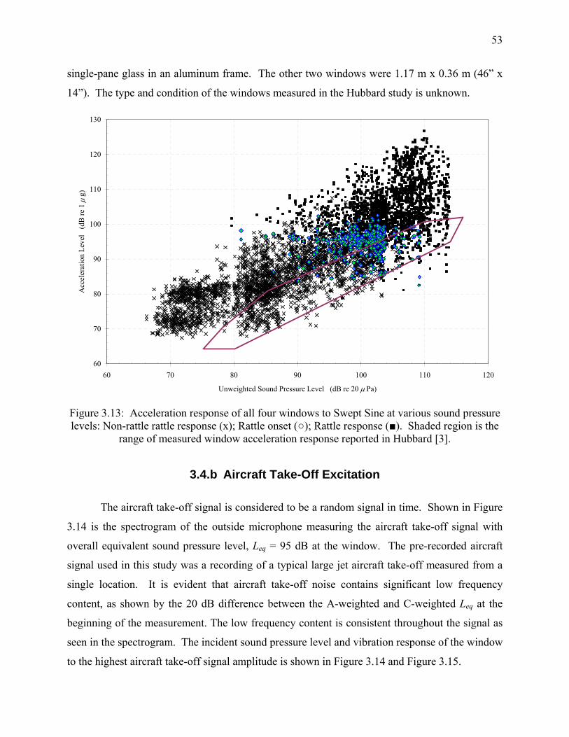
53
single-pane glass in an aluminum frame. The other two windows were 1.17 m x 0.36 m (46” x
14”). The type and condition of the windows measured in the Hubbard study is unknown.
60
70
80
90
100
110
120
130
60 70 80 90 100 110 120
Unweighted Sound Pressure Level (dB re 20 μ Pa)
Acc
eler
atio
n Le
vel
(dB
re 1
μg)
Figure 3.13: Acceleration response of all four windows to Swept Sine at various sound pressure levels: Non-rattle rattle response (x); Rattle onset (○); Rattle response (■). Shaded region is the
range of measured window acceleration response reported in Hubbard [3].
3.4.b Aircraft Take-Off Excitation
The aircraft take-off signal is considered to be a random signal in time. Shown in Figure
3.14 is the spectrogram of the outside microphone measuring the aircraft take-off signal with
overall equivalent sound pressure level, Leq = 95 dB at the window. The pre-recorded aircraft
signal used in this study was a recording of a typical large jet aircraft take-off measured from a
single location. It is evident that aircraft take-off noise contains significant low frequency
content, as shown by the 20 dB difference between the A-weighted and C-weighted Leq at the
beginning of the measurement. The low frequency content is consistent throughout the signal as
seen in the spectrogram. The incident sound pressure level and vibration response of the window
to the highest aircraft take-off signal amplitude is shown in Figure 3.14 and Figure 3.15.
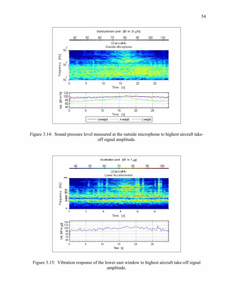
54
Figure 3.14: Sound pressure level measured at the outside microphone to highest aircraft take-off signal amplitude.
Figure 3.15: Vibration response of the lower east window to highest aircraft take-off signal amplitude.

55
Rattle events are identifiable as vertical highlights, indicating non-linear, broadband
response at times 6 s, 9 s, 11 s, 20 s, 22 s, and 26 s. Rattle onset typically occurred when the
acceleration level, Leq, was greater that 100 dB (re 1μg) or 0.1 grms. Audible rattle events are
tabulated in Table 3.2 for all aircraft take-off measurements.
Table 3.2: Audible rattle events during measurement for aircraft take-off signal.
Window Signal Amplitude, Incident Sound Level (dB)
Rattle Not Audible
Rattle Audible
70 X 80 X 90 X
Lower East
100 X 70 X 80 X 90 X
Lower West
100 X 70 X 80 X 90 X
Upper East
100 X 70 X 80 X 90 X
Upper West
100 X
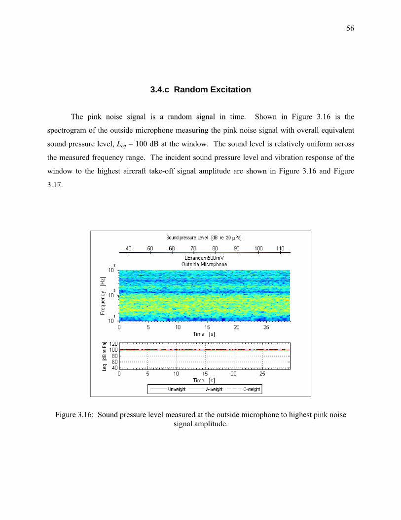
56
3.4.c Random Excitation
The pink noise signal is a random signal in time. Shown in Figure 3.16 is the
spectrogram of the outside microphone measuring the pink noise signal with overall equivalent
sound pressure level, Leq = 100 dB at the window. The sound level is relatively uniform across
the measured frequency range. The incident sound pressure level and vibration response of the
window to the highest aircraft take-off signal amplitude are shown in Figure 3.16 and Figure
3.17.
Figure 3.16: Sound pressure level measured at the outside microphone to highest pink noise signal amplitude.
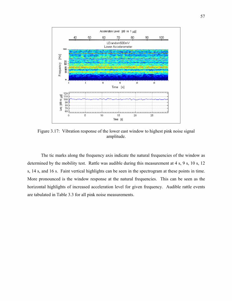
57
Figure 3.17: Vibration response of the lower east window to highest pink noise signal amplitude.
The tic marks along the frequency axis indicate the natural frequencies of the window as
determined by the mobility test. Rattle was audible during this measurement at 4 s, 9 s, 10 s, 12
s, 14 s, and 16 s. Faint vertical highlights can be seen in the spectrogram at these points in time.
More pronounced is the window response at the natural frequencies. This can be seen as the
horizontal highlights of increased acceleration level for given frequency. Audible rattle events
are tabulated in Table 3.3 for all pink noise measurements.

58
Table 3.3: Audible rattle events during measurement for pink noise signal.
Window Signal Amplitude, Incident Sound Level (dB)
Rattle Not Audible
Rattle Audible
70 X 80 X 90 X
Lower East
100 X 70 X 80 X 90 X
Lower West
100 X 70 X 80 X 90 X
Upper East
100 X 70 X 80 X 90 X
Upper West
100 X
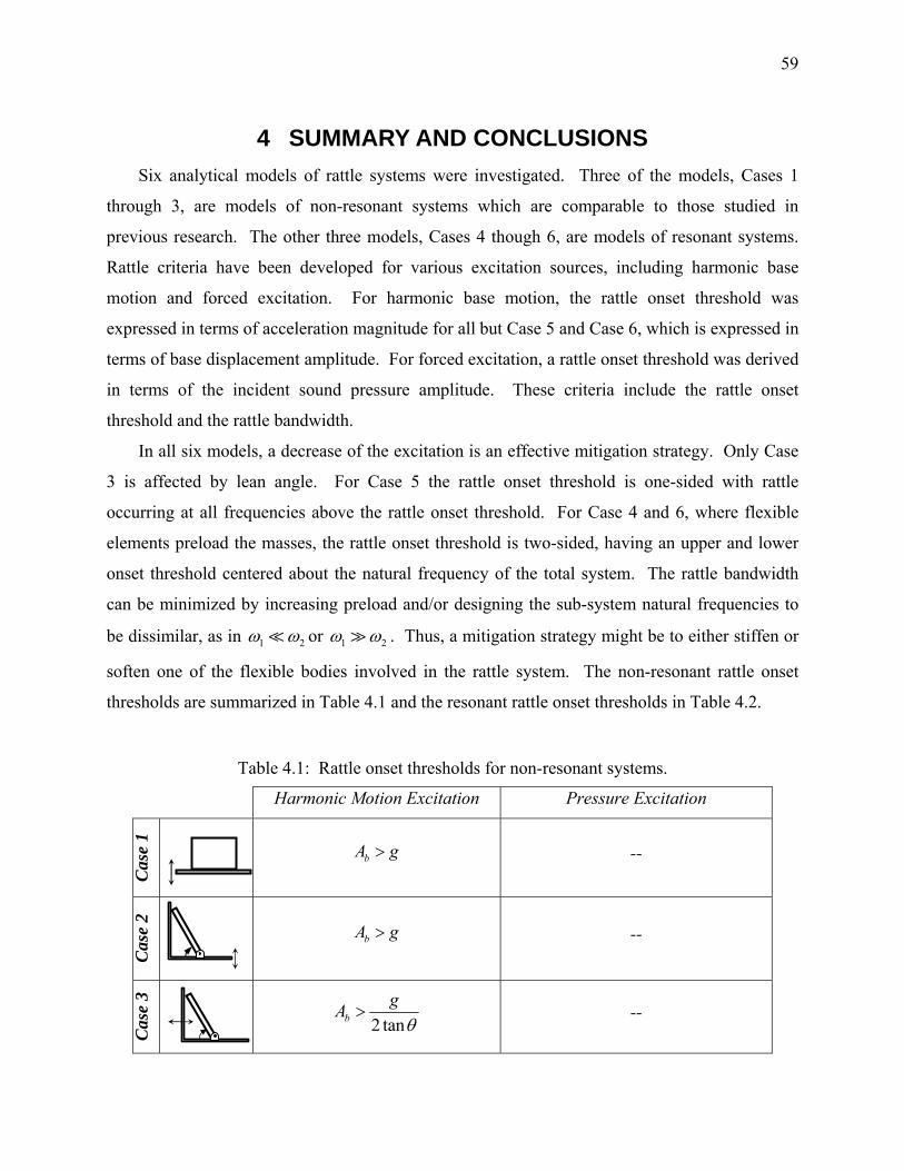
59
4 SUMMARY AND CONCLUSIONS Six analytical models of rattle systems were investigated. Three of the models, Cases 1
through 3, are models of non-resonant systems which are comparable to those studied in
previous research. The other three models, Cases 4 though 6, are models of resonant systems.
Rattle criteria have been developed for various excitation sources, including harmonic base
motion and forced excitation. For harmonic base motion, the rattle onset threshold was
expressed in terms of acceleration magnitude for all but Case 5 and Case 6, which is expressed in
terms of base displacement amplitude. For forced excitation, a rattle onset threshold was derived
in terms of the incident sound pressure amplitude. These criteria include the rattle onset
threshold and the rattle bandwidth.
In all six models, a decrease of the excitation is an effective mitigation strategy. Only Case
3 is affected by lean angle. For Case 5 the rattle onset threshold is one-sided with rattle
occurring at all frequencies above the rattle onset threshold. For Case 4 and 6, where flexible
elements preload the masses, the rattle onset threshold is two-sided, having an upper and lower
onset threshold centered about the natural frequency of the total system. The rattle bandwidth
can be minimized by increasing preload and/or designing the sub-system natural frequencies to
be dissimilar, as in 1 2ω ω or 1 2ω ω . Thus, a mitigation strategy might be to either stiffen or
soften one of the flexible bodies involved in the rattle system. The non-resonant rattle onset
thresholds are summarized in Table 4.1 and the resonant rattle onset thresholds in Table 4.2.
Table 4.1: Rattle onset thresholds for non-resonant systems.
Harmonic Motion Excitation Pressure Excitation
Cas
e 1
bA g> --
Cas
e 2
bA g> --
Cas
e 3
2 tanb
gAθ
> --

60
Table 4.2: Rattle onset thresholds for resonant systems.
Harmonic Motion Excitation Pressure Excitation C
ase
4
( ) ( )( )
( ) ( )
2 2 2
2 2 2
1 1
1 1
b
n
b
A g
A g
γ γ
ω ω
γ γ
− + −
< <
+ + −
--
Cas
e 5
( ) 2
,min 21 1p p
n b
y yY
ω γω
⎛ ⎞−⎛ ⎞⎜ ⎟> + − −⎜ ⎟ ⎜ ⎟⎝ ⎠ ⎝ ⎠
--
Cas
e 6
( )( )
( )
( )( )
( )
1 2
,min2
,min 2
,min2
,min 2
1 2
,min2
,min 2
,min2
,min 2
:
:
n
p p b
p p n b
n
p p b
p p n b
n
p p b
p p n b
n
p p b
p p n
y y Y
y y Y
y y Y
y y Y
y y Y
y y Y
y y Y
y y Yb
ω ω ω
ω ω
ω ω
ω ω
ω ω ω
ω ω
ω ω
ω ω
> >
− +
− +
< <
− −
− −
< <
− −
− −
< <
− +
− +
( )( ) ( )
( )
( )( ) ( )
( )( ) ( )
( )
( )( ) ( )
1 2
,min 1
2,min 2 1
,min 1
2,min 2 1
1 2
,min 1
2,min 2 1
,min 1
2,min 2 1
:
2
2
2
2
:
2
2
2
2
n
p p rms
p p n rms
n
p p rms
p p n rms
n
p p rms
p p n rms
n
p p rms
p p n rms
y y Sp k
y y Sp k
y y Sp k
y y Sp k
y y Sp k
y y Sp k
y y Sp k
y y Sp k
ω ω ω
ω ω
ω ω
ω ω
ω ω ω
ω ω
ω ω
ω ω
> >
− +
− +
< <
− −
− −
< <
− −
− −
< <
− +
− +
Rattle mitigation strategies are tabulated for the six rattle models in Table 4.3. In general,
reducing excitation and increasing preload will increase the rattle onset threshold and mitigate
rattle.

61
Table 4.3: Rattle mitigation strategies
Harmonic Motion Excitation Pressure Excitation C
ase
1
Reduce excitation. --
Cas
e 2
Reduce excitation. --
Cas
e 3
Reduce excitation.
Reduce angle. --
Cas
e 4
Increase pre-load.
Reduce excitation. --
Cas
e 5
Increase pre-load
Reduce excitation.
Decrease natural frequency
(reduce stiffness or increase
mass).
--
Cas
e 6
Increase pre-load.
Reduce excitation.
Soften or stiffen one flexible
body relative to the other.
Increase pre-load.
Reduce excitation.
Soften or stiffen one flexible
body relative to the other.
Experiments were conducted to verify the possible usefulness of the analytical rattle models.
Four windows prone to rattle were tested with three types of excitation signals (swept sine, pre-
recorded aircraft take-off, and random pink noise) at various signal strength amplitudes. The
rattle behavior of the window tested in the rattle experiment was in qualitative agreement with
the behavior predicted by the horizontal orientation Case 6 resonant rattle model. The rattle
62
occurred in a frequency band near the resonant frequencies of the window. This behavior is
consistent with predicted response of the analytical models. Several key observations may be
made. Rattle did not occur at any frequency for the lowest signal amplitude though resonant
behavior is evident. Thus for the right combination of parameters (excitation amplitude, preload,
material stiffness), rattle can be mitigated. Secondly, the rattle bandwidth increased for the
increasing excitation amplitude. Lastly, the rattle onset threshold (acceleration amplitude) for
the window was independent of frequency.
This study has investigated the mechanisms which cause rattle. Resonant rattle models
were developed which better represent the response of systems into rattle than previous non-
resonant rattle models.

63
5 LIST OF REFERENCES
[1] F. Kavarana, B. Rediers, Squeak and Rattle—State of the Art and Beyond, Sound and Vibration, pp. 56-64, April, (2001).
[2] L.C. Sutherland, S. Fidell, and A. Harris, Findings of the Low-Frequency Noise Expert Panel of the Rickfield-MAC Mitigation Agreement of 17 December 1998, Volumes I, II, and III, 30 September (2000).
[3] H.H. Hubbard, Noise Induced House Vibrations and Human Perception, Noise Control Engineering Journal, Vol. 19, pp.49-55, (1982).
[4] P.D. Schomer, S.D. Hottman, F.M. Kessler, and R.K. Kessler, Expedient Methods for Rattle-Proofing Certain Housing Components, USA-CERL, N-87/24, (1987).
[5] S.A. Clevenson, Experimental Determination of the Rattle of Simple Models, NASA Langley Research Center, NASA-TM-78756, (1978).
[6] H.D. Carden and W.H. Mayes, Measured Vibration Response Characteristics of Four Residential Structures Excited by Mechanical and Acoustical Loadings, NASA Langley Research Center, NASA-TN-D-5776, (1970).
[7] L.C. Sutherland, Low Frequency Response of Structures, Wyle Report, WR-82-18, (1982).
[8] L.C. Sutherland, B.H. Sharp, and R.A. Mantey, Preliminary Evaluation of Low Frequency Noise and Vibration Reduction Retrofit Concepts for Wood Frame Structures, Wyle Report, WR-83-26, (1983).
[9] ASTM E966, Standard Guide for Field Measurements of Airborne Sound Insulation of Building Façade Elements, American Society for Testing and Materials (ASTM), West Conshohocken, PA, (2002).
[10] ISO 140-5, Acoustics—Measurement of Sound Insulation in Buildings and of Building Elements—Part 5: Field Measurements of Airborne Sound Insulation of Façade Elements and Façades, International Organization for Standardization (ISO), Geneva, (1998).
[11] ISO 140-14, Acoustics—Measurement of Sound Insulation in Buildings and of Building Elements—Part 14: Guidelines for Special Situations in the Field, International Organization for Standardization (ISO), Geneva, (2004).
[12] H. Kess, MRIT and X-Modal Users Manual, Purdue University, December, (2004).
[13] J-.Y. Her and S-.R. Hsieh, A Review of Squeak and Rattle Prevention – A Personal Perspective, Proceedings of Noise-Con ‘98, Ypsilanti, MI, April 5-8 (1998).
[14] Staff-Langley Research Center: Concorde Noise-Induced Building Vibrations, John F. Kennedy International Airport, Report No. 3, NASA TM-78727, (April 1978).
[15] Staff-Langley Research Center: Concorde Noise-Induced Building Vibrations, International Airport Dulles—Final Report, NASA TM-74083 (September 1977).

64
6 APPENDICES

65
6.1 Appendix A: Experimental plots of rattle study
6.1.a Plots of Lower East (LE) window
6.1.a.i Background noise on Lower East (LE) window
Figure A.1: Room mic measuring background noise
Figure A.2: Outdoor mic measuring background noise
Figure A.3: Accelerometer measuring background noise

66
6.1.a.ii Aircraft take-off playback, Lower East (LE) window
Figure A.4: Room mic measuring aircraft take-off, (70 dBC at window)
Figure A.5: Outdoor mic measuring aircraft take-off, (70 dBC at window)
Figure A.6: Accelerometer measuring aircraft take-off, (70 dBC at window)

67
Figure A.7: Room mic measuring aircraft take-off, (80 dBC at window)
Figure A.8: Outdoor mic measuring aircraft take-off, (80 dBC at window)
Figure A.9: Accelerometer measuring aircraft take-off, (80 dBC at window)

68
Figure A.10: Room mic measuring aircraft take-off, (90 dBC at window)
Figure A.11: Outdoor mic measuring aircraft take-off, (90 dBC at window)
Figure A.12: Accelerometer measuring aircraft take-off, (90 dBC at window)

69
Figure A.13: Room mic measuring aircraft take-off, (100 dBC at window)
Figure A.14: Outdoor mic measuring aircraft take-off, (100 dBC at window)
Figure A.15: Accelerometer measuring aircraft take-off, (100 dBC at window)

70
6.1.a.iii Swept sine, Lower East (LE) window
Figure A.16: Room mic measuring swept sine, (70 dBC at window)
Figure A.17: Outdoor mic measuring swept sine, (70 dBC at window)
Figure A.18: Accelerometer measuring swept sine, (70 dBC at window)

71
Figure A.19: Room mic measuring swept sine, (80 dBC at window)
Figure A.20: Outdoor mic measuring swept sine, (80 dBC at window)
Figure A.21: Accelerometer measuring swept sine, (80 dBC at window)
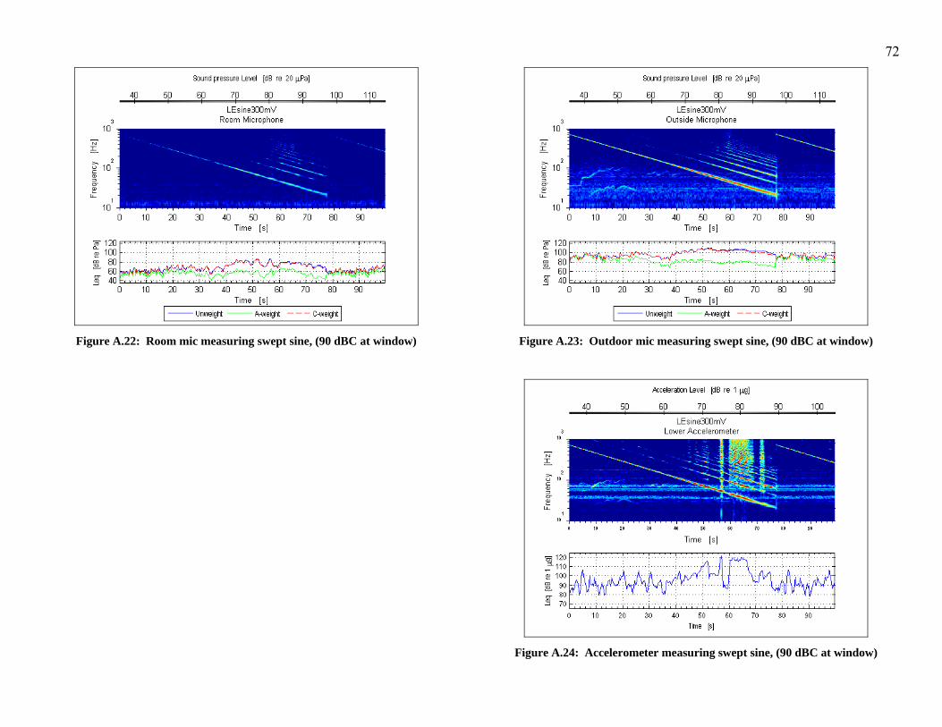
72
Figure A.22: Room mic measuring swept sine, (90 dBC at window)
Figure A.23: Outdoor mic measuring swept sine, (90 dBC at window)
Figure A.24: Accelerometer measuring swept sine, (90 dBC at window)

73
Figure A.25: Room mic measuring swept sine, (100 dBC at window)
Figure A.26: Outdoor mic measuring swept sine, (100 dBC at window)
Figure A.27: Accelerometer measuring swept sine, (100 dBC at window)

74
6.1.a.iv Random noise signal, Lower East (LE) window
Figure A.28: Room mic measuring random noise, (70 dBC at window)
Figure A.29: Outdoor mic measuring random noise, (70 dBC at window)
Figure A.30: Accelerometer measuring random noise, (70 dBC at window)

75
Figure A.31: Room mic measuring random noise, (80 dBC at window)
Figure A.32: Outdoor mic measuring random noise, (80 dBC at window)
Figure A.33: Accelerometer measuring random noise, (80 dBC at window)

76
Figure A.34: Room mic measuring random noise, (90 dBC at window)
Figure A.35: Outdoor mic measuring random noise, (90 dBC at window)
Figure A.36: Accelerometer measuring random noise, (90 dBC at window)
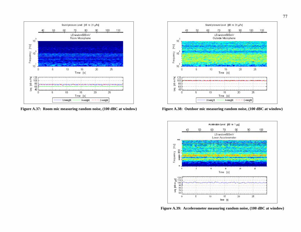
77
Figure A.37: Room mic measuring random noise, (100 dBC at window)
Figure A.38: Outdoor mic measuring random noise, (100 dBC at window)
Figure A.39: Accelerometer measuring random noise, (100 dBC at window)
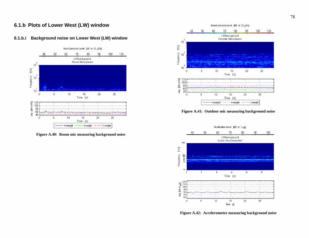
78
6.1.b Plots of Lower West (LW) window
6.1.b.i Background noise on Lower West (LW) window
Figure A.40: Room mic measuring background noise
Figure A.41: Outdoor mic measuring background noise
Figure A.42: Accelerometer measuring background noise
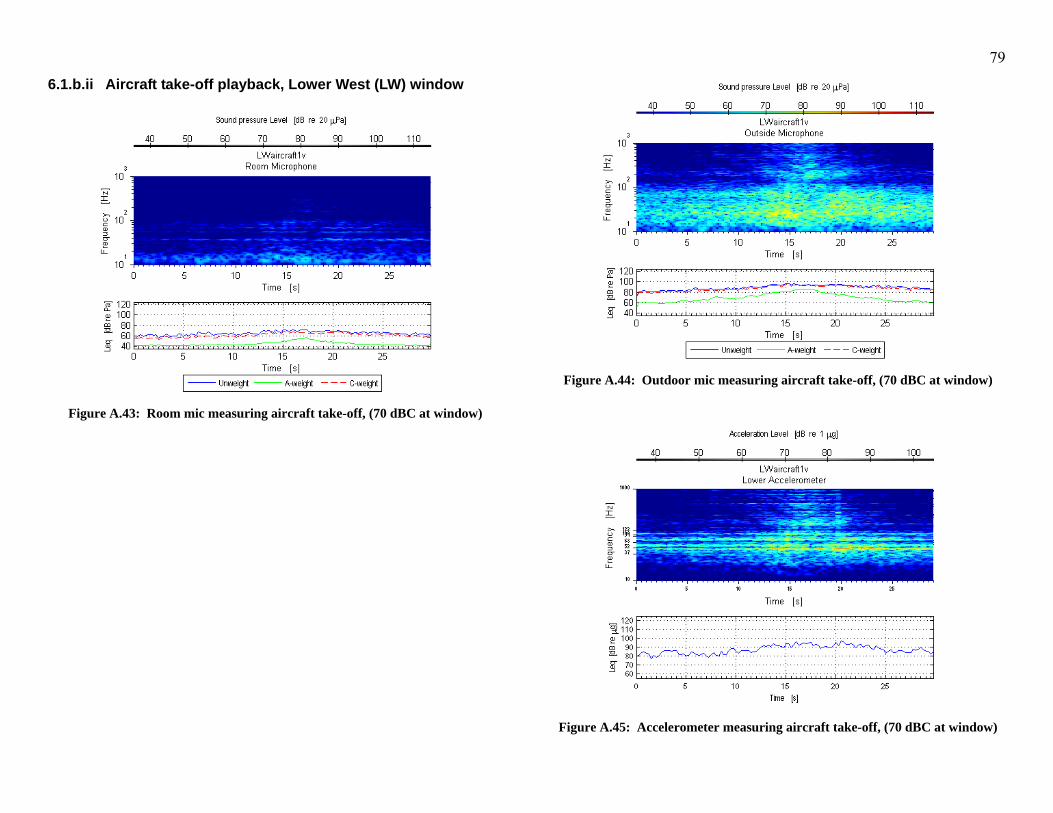
79
6.1.b.ii Aircraft take-off playback, Lower West (LW) window
Figure A.43: Room mic measuring aircraft take-off, (70 dBC at window)
Figure A.44: Outdoor mic measuring aircraft take-off, (70 dBC at window)
Figure A.45: Accelerometer measuring aircraft take-off, (70 dBC at window)

80
Figure A.46: Room mic measuring aircraft take-off, (80 dBC at window)
Figure A.47: Outdoor mic measuring aircraft take-off, (80 dBC at window)
Figure A.48: Accelerometer measuring aircraft take-off, (80 dBC at window)
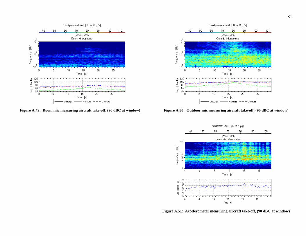
81
Figure A.49: Room mic measuring aircraft take-off, (90 dBC at window)
Figure A.50: Outdoor mic measuring aircraft take-off, (90 dBC at window)
Figure A.51: Accelerometer measuring aircraft take-off, (90 dBC at window)

82
Figure A.52: Room mic measuring aircraft take-off, (100 dBC at window)
Figure A.53: Outdoor mic measuring aircraft take-off, (100 dBC at window)
Figure 54: Accelerometer measuring aircraft take-off, (100 dBC at window)
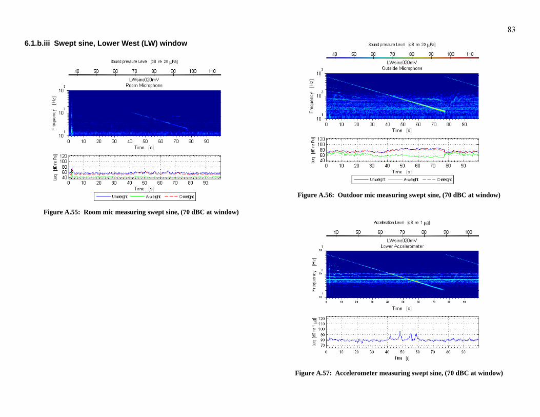
83
6.1.b.iii Swept sine, Lower West (LW) window
Figure A.55: Room mic measuring swept sine, (70 dBC at window)
Figure A.56: Outdoor mic measuring swept sine, (70 dBC at window)
Figure A.57: Accelerometer measuring swept sine, (70 dBC at window)

84
Figure A.58: Room mic measuring swept sine, (80 dBC at window)
Figure A.59: Outdoor mic measuring swept sine, (80 dBC at window)
Figure A.60: Accelerometer measuring swept sine, (80 dBC at window)

85
Figure A.61: Room mic measuring swept sine, (90 dBC at window)
Figure A.62: Outdoor mic measuring swept sine, (90 dBC at window)
Figure A.63: Accelerometer measuring swept sine, (90 dBC at window)

86
Figure A.64: Room mic measuring swept sine, (100 dBC at window)
Figure A.65: Outdoor mic measuring swept sine, (100 dBC at window)
Figure A.66: Accelerometer measuring swept sine, (100 dBC at window)

87
6.1.b.iv Random noise signal, Lower West (LW) window
Figure A.67: Room mic measuring random noise, (70 dBC at window)
Figure A.68: Outdoor mic measuring random noise, (70 dBC at window)
Figure A.69: Accelerometer measuring random noise, (70 dBC at window)

88
Figure A.70: Room mic measuring random noise, (80 dBC at window)
Figure A.71: Outdoor mic measuring random noise, (80 dBC at window)
Figure A.72: Accelerometer measuring random noise, (80 dBC at window)
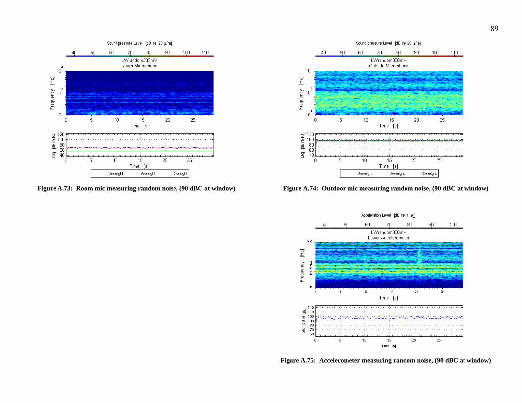
89
Figure A.73: Room mic measuring random noise, (90 dBC at window)
Figure A.74: Outdoor mic measuring random noise, (90 dBC at window)
Figure A.75: Accelerometer measuring random noise, (90 dBC at window)

90
Figure A.76: Room mic measuring random noise, (100 dBC at window)
Figure A.77: Outdoor mic measuring random noise, (100 dBC at window)
Figure A.78: Accelerometer measuring random noise, (100 dBC at window)

91
6.1.c Plots of Upper East (UE) window
6.1.c.i Background noise on Upper East (UE) window
Figure A.79: Room mic measuring background noise
Figure A.80: Outdoor mic measuring background noise
Figure A.81: Accelerometer measuring background noise

92
6.1.c.ii Aircraft take-off playback, Upper East (UE) window
Figure A.82: Room mic measuring aircraft take-off, (70 dBC at window)
Figure A.83: Outdoor mic measuring aircraft take-off, (70 dBC at window)
Figure A.84: Accelerometer measuring aircraft take-off, (70 dBC at window)

93
Figure A.85: Room mic measuring aircraft take-off, (80 dBC at window)
Figure A.86: Outdoor mic measuring aircraft take-off, (80 dBC at window)
Figure A.87: Accelerometer measuring aircraft take-off, (80 dBC at window)

94
Figure A.88: Room mic measuring aircraft take-off, (90 dBC at window)
Figure A.89: Outdoor mic measuring aircraft take-off, (90 dBC at window)
Figure A.90: Accelerometer measuring aircraft take-off, (90 dBC at window)

95
Figure A.91: Room mic measuring aircraft take-off, (100 dBC at window)
Figure A.92: Outdoor mic measuring aircraft take-off, (100 dBC at window)
Figure A.93: Accelerometer measuring aircraft take-off, (100 dBC at window)
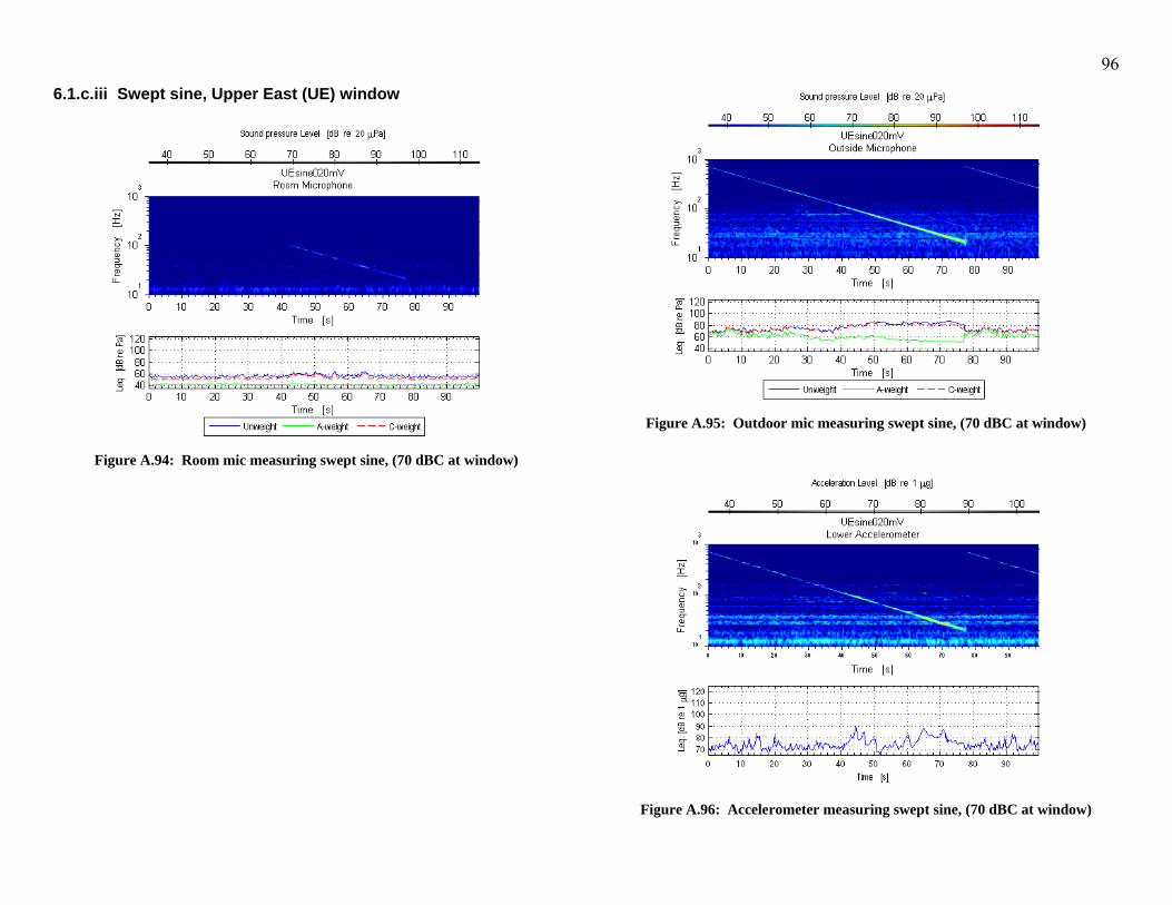
96
6.1.c.iii Swept sine, Upper East (UE) window
Figure A.94: Room mic measuring swept sine, (70 dBC at window)
Figure A.95: Outdoor mic measuring swept sine, (70 dBC at window)
Figure A.96: Accelerometer measuring swept sine, (70 dBC at window)

97
Figure A.97: Room mic measuring swept sine, (80 dBC at window)
Figure A.98: Outdoor mic measuring swept sine, (80 dBC at window)
Figure A.99: Accelerometer measuring swept sine, (80 dBC at window)
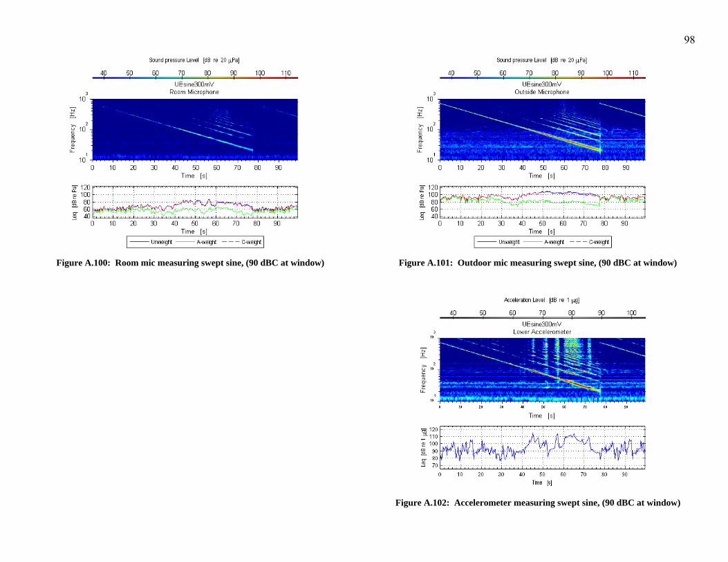
98
Figure A.100: Room mic measuring swept sine, (90 dBC at window)
Figure A.101: Outdoor mic measuring swept sine, (90 dBC at window)
Figure A.102: Accelerometer measuring swept sine, (90 dBC at window)

99
Figure A.103: Room mic measuring swept sine, (100 dBC at window)
Figure A.104: Outdoor mic measuring swept sine, (100 dBC at window)
Figure A.105: Accelerometer measuring swept sine, (100 dBC at window)

100
6.1.c.iv Random noise signal, Upper East (UE) window
Figure A.106: Room mic measuring random noise, (70 dBC at window)
Figure A.107: Outdoor mic measuring random noise, (70 dBC at window)
Figure A.108: Accelerometer measuring random noise, (70 dBC at window)
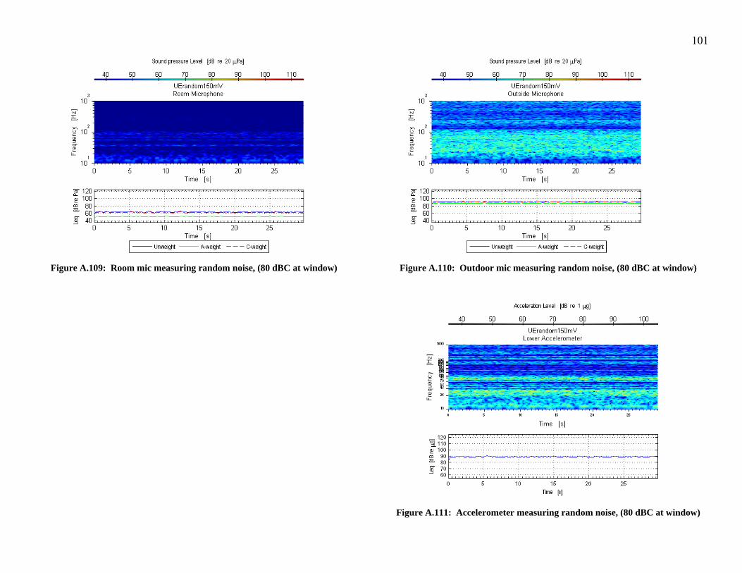
101
Figure A.109: Room mic measuring random noise, (80 dBC at window)
Figure A.110: Outdoor mic measuring random noise, (80 dBC at window)
Figure A.111: Accelerometer measuring random noise, (80 dBC at window)

102
Figure A.112: Room mic measuring random noise, (90 dBC at window)
Figure A.113: Outdoor mic measuring random noise, (90 dBC at window)
Figure A.114: Accelerometer measuring random noise, (90 dBC at window)

103
Figure A.115: Room mic measuring random noise, (100 dBC at window)
Figure A.116: Outdoor mic measuring random noise, (100 dBC at window)
Figure A.117: Accelerometer measuring random noise, (100 dBC at window)

104
6.1.d Plots of Upper West (UW) window
6.1.d.i Background noise on Upper West (UW) window
Figure A.118: Room mic measuring background noise
Figure A.119: Outdoor mic measuring background noise
Figure A.120: Accelerometer measuring background noise
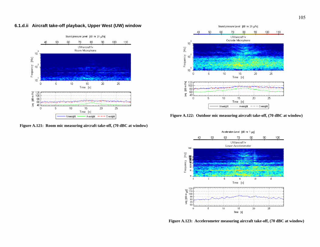
105
6.1.d.ii Aircraft take-off playback, Upper West (UW) window
Figure A.121: Room mic measuring aircraft take-off, (70 dBC at window)
Figure A.122: Outdoor mic measuring aircraft take-off, (70 dBC at window)
Figure A.123: Accelerometer measuring aircraft take-off, (70 dBC at window)

106
Figure A.124: Room mic measuring aircraft take-off, (80 dBC at window)
Figure A.125: Outdoor mic measuring aircraft take-off, (80 dBC at window)
Figure A.126: Accelerometer measuring aircraft take-off, (80 dBC at window)
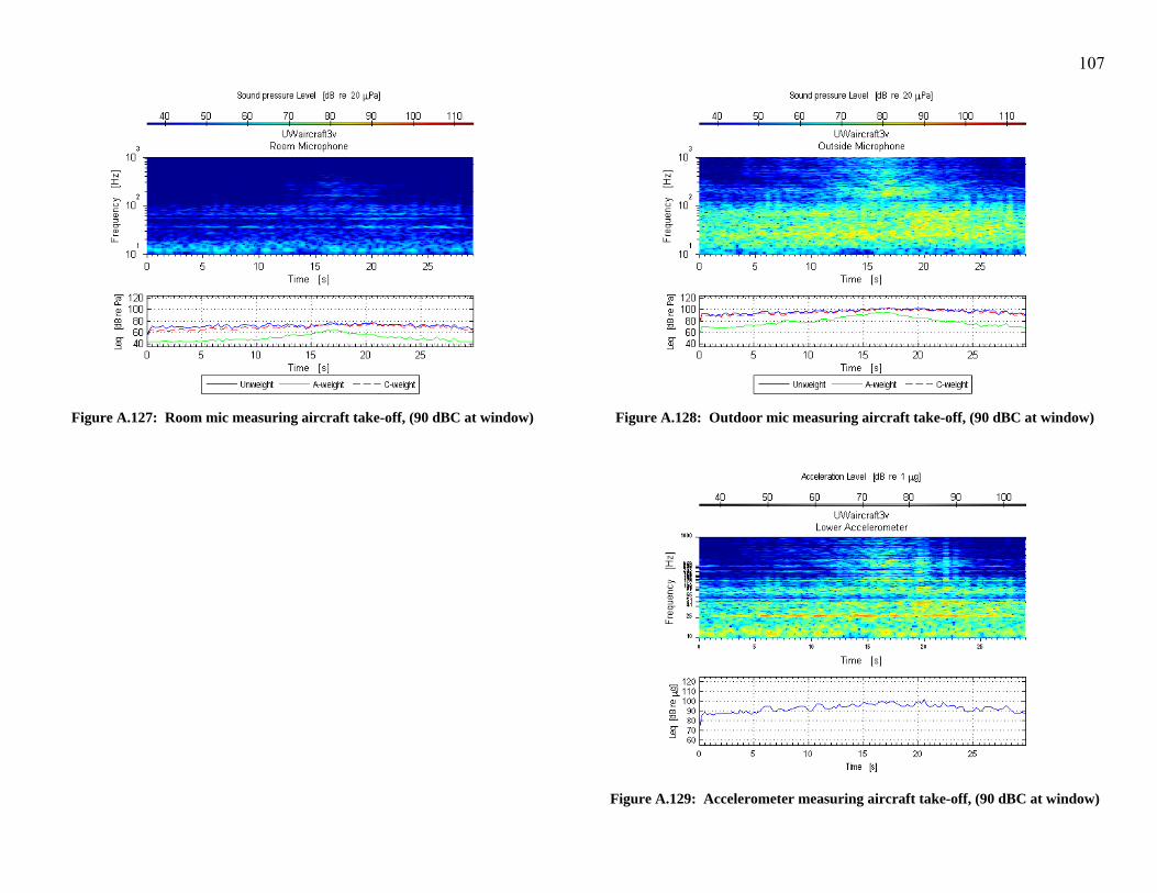
107
Figure A.127: Room mic measuring aircraft take-off, (90 dBC at window)
Figure A.128: Outdoor mic measuring aircraft take-off, (90 dBC at window)
Figure A.129: Accelerometer measuring aircraft take-off, (90 dBC at window)
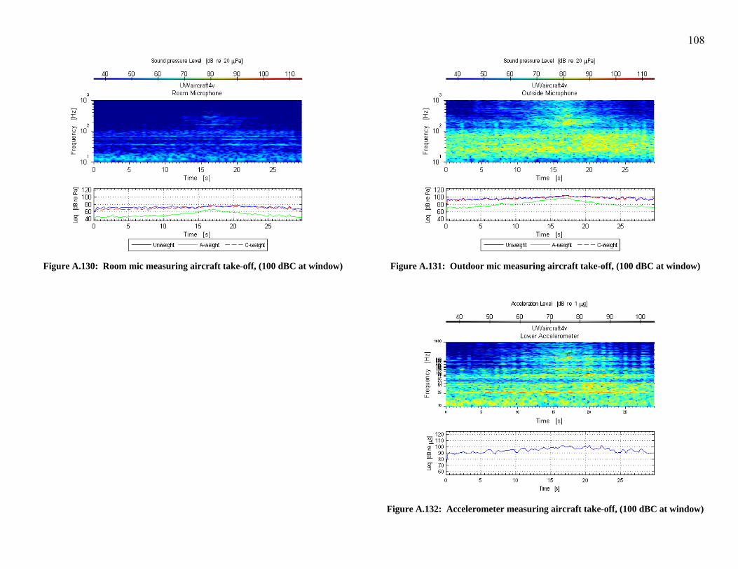
108
Figure A.130: Room mic measuring aircraft take-off, (100 dBC at window)
Figure A.131: Outdoor mic measuring aircraft take-off, (100 dBC at window)
Figure A.132: Accelerometer measuring aircraft take-off, (100 dBC at window)

109
6.1.d.iii Swept sine, Upper West (UW) window
Figure A.133: Room mic measuring swept sine, (70 dBC at window)
Figure A.134: Outdoor mic measuring swept sine, (70 dBC at window)
Figure A.135: Accelerometer measuring swept sine, (70 dBC at window)

110
Figure A.136: Room mic measuring swept sine, (80 dBC at window)
Figure A.137: Outdoor mic measuring swept sine, (80 dBC at window)
Figure A.138: Accelerometer measuring swept sine, (80 dBC at window)
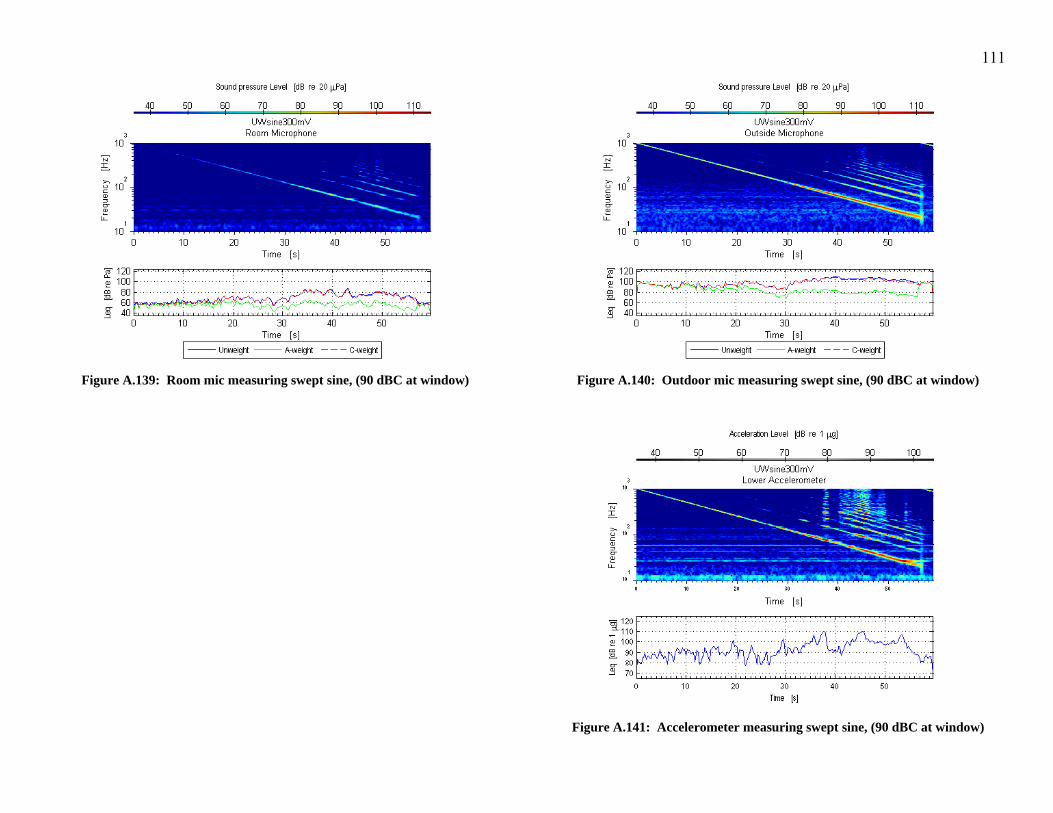
111
Figure A.139: Room mic measuring swept sine, (90 dBC at window)
Figure A.140: Outdoor mic measuring swept sine, (90 dBC at window)
Figure A.141: Accelerometer measuring swept sine, (90 dBC at window)

112
Figure A.142: Room mic measuring swept sine, (100 dBC at window)
Figure A.143: Outdoor mic measuring swept sine, (100 dBC at window)
Figure A.144: Accelerometer measuring swept sine, (100 dBC at window)

113
6.1.d.iv Random noise signal, Upper West (UW) window
Figure A.145: Room mic measuring random noise, (70 dBC at window)
Figure A.146: Outdoor mic measuring random noise, (70 dBC at window)
Figure A.147: Accelerometer measuring random noise, (70 dBC at window)

114
Figure A.148: Room mic measuring random noise, (80 dBC at window)
Figure A.149: Outdoor mic measuring random noise, (80 dBC at window)
Figure A.150: Accelerometer measuring random noise, (80 dBC at window)
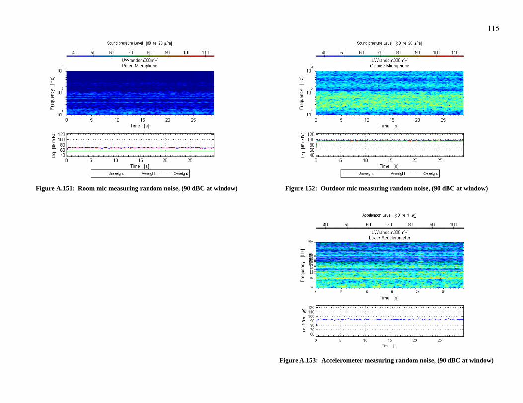
115
Figure A.151: Room mic measuring random noise, (90 dBC at window)
Figure 152: Outdoor mic measuring random noise, (90 dBC at window)
Figure A.153: Accelerometer measuring random noise, (90 dBC at window)

116
Figure A.154: Room mic measuring random noise, (100 dBC at window) Figure A.155: Outdoor mic measuring random noise, (100 dBC at window)
Figure A.156: Accelerometer measuring random noise, (100 dBC at window)

117
6.2 Appendix B: Measured Window Rattle Thresholds
60
70
80
90
100
110
120
130
20 30 40 50 60 70 80 90 100
Input Frequency (Hz)
Acc
eler
atio
n Le
vel
(dB
re 1
mg)
Figure B.1: Response of the lower east window to four swept sine signal strengths; 70 dBC blue, 80 dBC green, 90 dBC orange, 100 dBC black. Bolded
line-style indicates input frequencies at which rattle occurred.
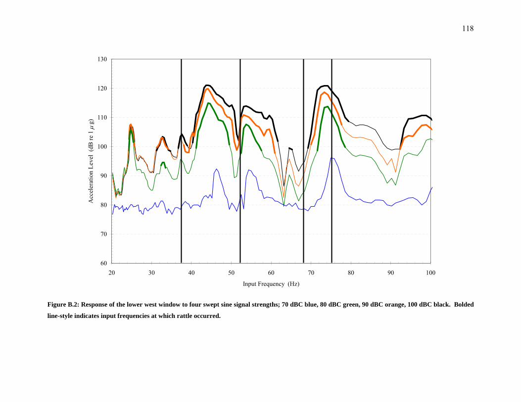
118
60
70
80
90
100
110
120
130
20 30 40 50 60 70 80 90 100
Input Frequency (Hz)
Acc
eler
atio
n Le
vel
(dB
re 1
μg)
Figure B.2: Response of the lower west window to four swept sine signal strengths; 70 dBC blue, 80 dBC green, 90 dBC orange, 100 dBC black. Bolded
line-style indicates input frequencies at which rattle occurred.
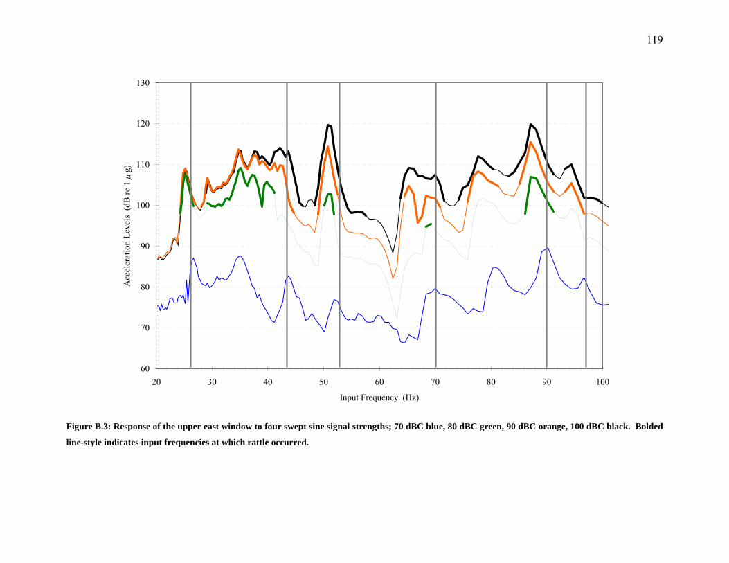
119
60
70
80
90
100
110
120
130
20 30 40 50 60 70 80 90 100
Input Frequency (Hz)
Acc
eler
atio
n Le
vels
(dB
re 1
μg)
Figure B.3: Response of the upper east window to four swept sine signal strengths; 70 dBC blue, 80 dBC green, 90 dBC orange, 100 dBC black. Bolded
line-style indicates input frequencies at which rattle occurred.

120
60
70
80
90
100
110
120
130
20 30 40 50 60 70 80 90 100
Input Frequency (Hz)
Acc
eler
atio
n Le
vel
(dB
re 1
μg)
Figure B.4: Response of the upper west window to four swept sine signal strengths; 70 dBC blue, 80 dBC green, 90 dBC orange, 100 dBC black. Bolded
line-style indicates input frequencies at which rattle occurred.