THE GENESIS TRAJECTORY AND HETEROCLINIC

CONNECTIONS

Wang Sang Koon�, Martin W. Loy, Jerrold E. Marsden�and Shane D. Ross�

Genesis will be NASA's �rst robotic sample return mission. The purpose

of this mission is to collect solar wind samples for two years in an L1 halo

orbit and return them to the Utah Test and Training Range (UTTR) for

mid-air retrieval by helicopters. To do this, the Genesis spacecraft makes

an excursion into the region around L2. This transfer between L1 and

L2 requires no deterministic maneuvers and is provided by the existence

of heteroclinic cycles de�ned below. The Genesis trajectory was designed

with the knowledge of the conjectured existence of these heteroclinic cycles.

We now have provided the �rst systematic, semi-analytic construction of

such cycles. The heteroclinic cycle provides several interesting applications

for future missions. First, it provides a rapid low-energy dynamical channel

between L1 and L2 such as used by the Genesis Discovery Mission. Second,

it provides a dynamical mechanism for the temporary capture of objects

around a planet without propulsion. Third, interactions with the Moon.

Here we speak of the interactions of the Sun-Earth Lagrange point dynamics

with the Earth-Moon Lagrange point dynamics. We motivate the discussion

using Jupiter comet orbits as examples. By studying the natural dynamics

of the Solar System, we enhance current and future space mission design.

INTRODUCTION

The key feature of the Genesis trajectory (see Figure 1) is the Return Trajectory which

makes a 3 million km excursion between L1 and L2 in order to reach UTTR during day-

light hours. The extraordinary thing about this 5 month excursion is that it requires no

deterministic maneuvers! In the language of dynamical systems theory, this transfer is said

to shadow a heteroclinic connection between the L1 and L2 regions.

There is, in fact, a vast theory about heteroclinic dynamics which among other things are

the generators of deterministic chaos in a dynamical system. Our recent work (Koon et al.1)

provides a precise theory of how heteroclinic dynamics arise in the context of the planar

circular restricted three-body problem (PCR3BP). In this paper, we apply this theory

to explain how the Genesis return trajectory works. This provides the beginnings of a

systematic approach to the design and generation of this type of trajectories. In the not

too distant future, automation of this process will be possible based on this approach. The

eventual goal is for the on board autonomous navigation of this type of low-energy Earth

sample return missions. But in fact, as we will show, this dynamics a�ects a much greater

class of new mission concepts.

�Control and Dynamical Systems, California Institute of Technology, Pasadena, CA 91125.yNavigation and Flight Mechanics, Jet Propulsion Laboratory, Pasadena, CA 91109.

1

View from North Ecliptic (+ Z-axis)

View from Anti-Earth Velocity (- Y-axis) View from Anti-Sun (+ X-axis)

Axis, in millions of kilometers:X = Sun-Earth Line, positive anti-sunY = (Z) X (X)Z = Ecliptic Normal (North)

Figure 1: The Genesis trajectory in Sun-Earth rotating frame.

To motivate the discussion and to provide an independent example from nature, we

examine the orbit of the comets, Oterma and Gehrels 3. We want to understand how

heteroclinic dynamics work in nature in order to develop and verify our theory. An impor-

tant theme in our work is to learn from nature because it seems that nature has already

found the best solution. Whatever we can glean from natural phenomena will contribute

immeasurably to the development of new trajectory and mission concepts. In particular,

the understanding of the structure of the heteroclinic and homoclinic orbits has given us

new insights into the transport mechanisms within the Solar System which can be utilized

for space trajectory design.

We will explain the key theorem from Koon et al.1 and apply it to the \temporary

capture mechanism" in the astrodynamics context. Of course, this theorem has more to

say about the complex orbital dynamics in this regime. It seems that the region of phase

space between L1 and L2 is full of dynamical channels like a complex system of wormholes

or tunnels. These channels exist throughout the Solar System in a vast network connecting

all the planets and their satellites (see Lo and Ross2�3). Together, they provide a network

of low-energy trajectories which may be used for new mission concepts. Although these

hidden passageways may be new to us, they have been well trodden by comets and asteroids

perhaps since the birth of the Solar System. We apply our understanding of these dynamical

channels to a new class of missions which we call \The Petit Grand Tour". The Petit Grand

Tour combines the temporary capture mechanism with the concept of the interplanetary

2

network of dynamical channels (or dynamical wormholes) to provide a low-energy mission

to tour the moons of Jupiter (or Saturn) in any desired sequence.

HETEROCLINIC CONNECTIONS AND CYCLES

The goal of the Genesis Mission is to return to UTTR all of the solar wind samples collected

over four revolutions (two years) in an L1 halo orbit (see Lo et al.4 and references therein).

The mid-air retrieval of the ballistic sample return capsule by helicopters requires that the

entry must occur during daylight. But the natural dynamics of an L1 halo orbit require a

night-side return. In order to achieve the day-side entry within a reasonable �V budget,

an excursion into the L2 region is necessary which added two months to the return phase.

A heteroclinic connection, H, also called a heteroclinic trajectory, is an asymptotic tra-

jectory which connects two periodic orbits which we denote by A and B for this discussion.

In the event A and B are the same periodic orbit, H is called a homoclinic orbit. H is a

theoretical construct of great importance both in theory and in practical applications. We

examine some of the key features of these orbits. It takes H in�nite time to wind o� from

A to transfer to B. Once near the vicinity of B, it takes H an in�nite time to wind onto B.

They were studied intensely by Poincar�e and were central to his discovery of chaos in the

3 body problem. Practically, of course, we are never able to compute the real H just as we

are never able to compute the real periodic orbits of any nonlinear system. However, what

we are able to compute are neighboring trajectories, H's, which \shadow" H to any desired

accuracy (within machine accuracy) for the particular problem at hand.

Now a slight diversion on our notation which we will keep to a minimum. We denote

a heteroclinic orbit between A and B by HAB and a heteroclinic orbit between B and A

by HBA. In particular, a homoclinic orbit of A is denoted by HAA. We distinguish the

theoretical orbit, H, and its numerical shadow, H, by the script and block fonts respectively.

Returning to our main discussion, when we have a heteroclinic orbit between A and B and a

heteroclinic orbit between B and A, the two orbits fHAB;HBAg form a heteroclinic cycle. In

particular, homoclinic orbits are already cycles. The importance of cycles both theoretically

and practically will be discussed shortly. We shall see that they are very important indeed.

Of course, the existence of heteroclinic behavior was generally known to the halo mission

community previously. Typically when integrating an L1 halo orbit for too long, it escapes

the vicinity of the halo orbit and sometimes returns towards Earth before continuing to

wind around L2. Thus the phenomenon is easily observed in numerical experiments. The

WIND Mission was the �rst to use this heteroclinic behavior between L1 and L2 (Sharer el

al.5). Howell and Barden6 made a more formal study of heteroclinic connections and found

a free connection between a halo orbit and a lissajous orbit using numerical search.

Koon, Lo, Marsden and Ross1 studied the problem of PCR3BP and used the more

systematic method of Poincar�e sections from dynamical systems theory to produce hetero-

clinic orbits between two Lyapunov orbits (periodic orbits around L1 and L2 in the plane).

The method of Poincar�e section reduces the problem by one dimension thereby rendering

the problem more tractable. Futhermore, there is a substantial body of known results on

Poincar�e sections from dynamical systems theory which provide additional knowledge and

insight into the speci�cs of the dynamics. This knowledge and insight provide the founda-

tion for new mission concepts and for the optimization of current mission designs discussed

in this paper.

3

We conclude this section by emphasizing the importance of these seemingly esoteric

theoretical constructs, the H and H orbits. Their importance in astrodynamics is two-fold:

(1) to simplify computation, and (2) to generate new mission concepts. Their importance

to computation is perhaps best illustrated by the process used to compute the Genesis halo

orbit which we denote by G. We start the process with a theoretical model lissajous orbit,

G, speci�ed by amplitudes and phase angles. We produce an analytic approximation, G1

using a 3rd order analytic expansion. Next we produce a di�erentially corrected lissajous

orbit, G2, from G1. Finally, starting with G2, we apply the various mission constraints and

di�erentially correct for the Genesis halo orbit, G. To summarize, the theoretical model

orbit, G, is the starting point from which practical orbits may be constructed via the contin-

uation process using a series of numerical computations. In the same way, the Genesis Earth

return trajectory was computed using heteroclinic-like orbits as initial models. Therefore,

advances in the theory and computation of these orbits are essential to the simpli�cation

and eventual automation of this complex process of continuation. It is remarkable to think

how Poincar�e was able to see all of these complex issues and actually perform continuation

calculations of orbits without the bene�t of modern computers. The discussion of their

importance to new mission concepts occupies the rest of this paper.

The Three Body Problem

We start with the PCR3BP as our �rst model of the mission design space, the equations of

motion for which in rotating frame with normalized coordinates are:

�x� 2 _y = x; �y + 2 _x = y;

where

=x2 + y2

2+

1� �

rS+

�

rJ+�(1� �)

2:

The subscripts of denote partial di�erentiation in the variable and dots over the variables

are time derivatives. The variables rS; rJ , are the distances from (x; y) to the two primary

bodies, which we refer to generically as the Sun and Jupiter, respectively.

The coordinates of the equations use standard PCR3BP conventions: the sum of the

mass of the Sun and Jupiter is normalized to 1 with the mass of Jupiter set to �; the distance

between the Sun and Jupiter is normalized to 1; and the angular velocity of Jupiter around

the Sun is normalized to 1. Hence in this model, Jupiter is moving around the Sun in a

circular orbit with period 2�. The rotating coordinates, following standard astrodynamic

conventions, are de�ned as follows: the origin is set at the Sun-Jupiter barycenter; the

x-axis is de�ned by the Sun-Jupiter line with Jupiter on the positive x-axis; the (x; y)-plane

is the plane of the orbit of Jupiter around the Sun (see Figure 2).

Although the PCR3BP has 3 collinear libration points which are unstable, for the cases

of interest to mission design, we examine only L1 and L2 in this paper. These equations

are autonomous and can be put into Hamiltonian form with 2 degrees of freedom. It has

an energy integral called the Jacobi constant which provides 3-dimensional constant energy

surfaces:

C = �( _x2 + _y2) + 2(x; y):

The power of dynamical systems theory is that it is able to provide additional structures

within the energy surface and characterize the di�erent regimes of motions.

4

-10 -8 -6 -4 -2 0 2 4 6 8 10-10

-8

-6

-4

-2

0

2

4

6

8

10

x (AU, Sun-Jupiter rotating frame)

y (A

U, S

un-J

upite

r ro

tatin

g fr

ame)

L4

L5

L2L1L3S J

Jupiter’s orbit-10 -8 -6 -4 -2 0 2 4 6 8 10

-10

-8

-6

-4

-2

0

2

4

6

8

10

S J

x (AU, Sun-Jupiter rotating frame)

y (A

U, S

un-J

upite

r ro

tatin

g fr

ame)

(a) (b)

Oterma’s orbit

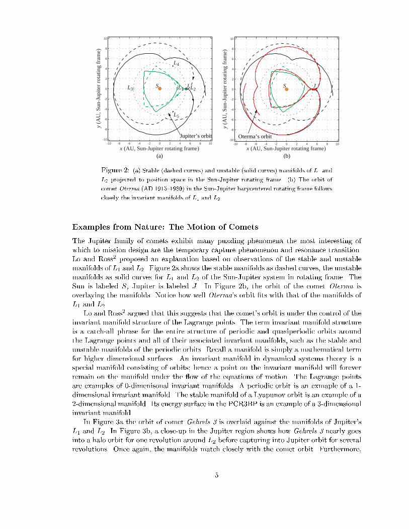
Figure 2: (a) Stable (dashed curves) and unstable (solid curves) manifolds of L1 and

L2 projected to position space in the Sun-Jupiter rotating frame. (b) The orbit of

comet Oterma (AD 1915{1980) in the Sun-Jupiter barycentered rotating frame follows

closely the invariant manifolds of L1 and L2.

Examples from Nature: The Motion of Comets

The Jupiter family of comets exhibit many puzzling phenomena the most interesting of

which to mission design are the temporary capture phenomenon and resonance transition.

Lo and Ross2 proposed an explanation based on observations of the stable and unstable

manifolds of L1 and L2. Figure 2a shows the stable manifolds as dashed curves, the unstable

manifolds as solid curves for L1 and L2 of the Sun-Jupiter system in rotating frame. The

Sun is labeled S, Jupiter is labeled J . In Figure 2b, the orbit of the comet Oterma is

overlaying the manifolds. Notice how well Oterma's orbit �ts with that of the manifolds of

L1 and L2.

Lo and Ross2 argued that this suggests that the comet's orbit is under the control of the

invariant manifold structure of the Lagrange points. The term invariant manifold structure

is a catch-all phrase for the entire structure of periodic and quasiperiodic orbits around

the Lagrange points and all of their associated invariant manifolds, such as the stable and

unstable manifolds of the periodic orbits. Recall a manifold is simply a mathematical term

for higher dimensional surfaces. An invariant manifold in dynamical systems theory is a

special manifold consisting of orbits; hence a point on the invariant manifold will forever

remain on the manifold under the ow of the equations of motion. The Lagrange points

are examples of 0-dimenisonal invariant manifolds. A periodic orbit is an exmaple of a 1-

dimensional invariant manifold. The stable manifold of a Lyapunov orbit is an example of a

2-dimensional manifold. Its energy surface in the PCR3BP is an example of a 3-dimensional

invariant manifold.

In Figure 3a the orbit of comet Gehrels 3 is overlaid against the manifolds of Jupiter's

L1 and L2. In Figure 3b, a close-up in the Jupiter region shows how Gehrels 3 nearly goes

into a halo orbit for one revolution around L2 before capturing into Jupiter orbit for several

revolutions. Once again, the manifolds match closely with the comet orbit. Furthermore,

5

(a) (b)

Figure 3: (a) The orbit of Gehrels 3 overlaying the manifolds of Jupiter's L1 and L2.

Stable manifolds are dashed lines, unstable manifolds are solid lines. (b) The orbit of

Gehrels 3 in the Jupiter region showing temporary captures and halo orbits.

the temporary capture of the comet by Jupiter suggests the possibilities of low-energy

capture for interplanetary missions.

Based on the invariant manifold approach suggested by Lo and Ross2, Koon et al.1 gives

a systematic and mathematically rigorous explanation of this dynamics. In addition to a

more complete global qualitative picture, it also provides computational and predictive ca-

pabilities. It provides an algorithm based on standard Poincar�e section methods to compute

heteroclinic orbits. It provides the rudiments for the calculation of transport probabilities

based on lobe dynamics theory (see Wiggins7, Meiss8). Previous mission design work using

heteroclinic dynamics were based on ad hoc numerical search and exploration. But the

new computation tools of Koon et al.1 enable the mission designer to construct heteroclinic

trajectories in a systematic fashion instead of using a blind and brute force search. The

results are promising and more research and development work remains before this process

may be fully automated.

The Orbit Classes Near L1 and L2.

The work of Lo and Ross2 demonstrated that the dynamics of the L1 and L2 region is

extremely important for the understanding of many disparate dynamical phenomena in

the Solar System and also for space mission design. In order to better understand the

dynamics of this region, we now review the work of Conley9 and McGehee10 which provide

an essential characterization of the orbital structure near L1 and L2. McGehee also proved

the existence of homoclinic orbits in the interior and exterior regions. Llibre, Martinez, and

Sim�o11 showed that the homoclinic orbits of L1 in the interior region are transversal. They

used symbolic dynamics to prove a theorem for orbital motions in the interior and Jupiter

region. One of the key results in Koon et al.1 is the completion of this picture with the

computation of heteroclinic cycles in the Jupiter region between L1 and L2. We will refer to

the various regions by the following short hand: S for the interior region which contains the

Sun, J for the Jupiter region which contains the planet, X for the exterior region outside

6

the planet's orbit.

S JL1 L2

ExteriorRegion (X)

Interior (Sun)Region (S)

JupiterRegion (J)

ForbiddenRegion

L2

Figure 4: (a) Hill's region (schematic, the region in white) connecting the interior

region, the capture region, and the exterior region. (b) Expanded view of the L2

region showing a periodic orbit, a typical asymptotic orbit, two transit orbits and two

non-transit orbits.

Figure 4 schematically summarizes the key results of Conley and McGehee. For an

energy value just about that of L2, the Hill's region is the projection of the energy surface

from the phase space onto the con�guration space, i.e. the xy-plane. This is represented by

the white space in Figure 4a. The grey region is energetically forbidden. In other words,

with the given energy, our spacecraft can only explore the white region. More energy is

required to enter the grey Forbidden region.

Figure 4b is a blow-up of the L2 region to indicate the existence of four di�erent classes

of orbits. The �rst class is a single periodic orbit with the given energy, the planar Lya-

punov orbit around L2. The second class represented by a spiral is an asymptotic orbit

winding onto the periodic orbit. This is an orbit on the stable manifold of the Lyapunov

orbit. Similarly, although not shown, are orbits which wind o� the Lyapunov orbit to form

the unstable manifold. The third class are transit orbits which pass through the Jupiter

region between the S and X regions. Lastly, the fourth class consists of orbits which are

temporarily trapped in the S or X regions.

Let us examine the stable and unstable manifold of a Lyapunov orbit as shown in Figure

5. Of course, only a very small portion of the manifolds are plotted. Notice the X-pattern

typical of a saddle formed by the manifolds. This is reminiscent of the X-pattern of the

manifolds of the Lagrange points in Figure 3b. It is precisely in this sense that we say

the manifolds of the Lagange points are \genetic"; they characterize the essential shapes

and dynamics of things to come when more complexity such as periodic orbits and their

manifolds are introduced. Thus, by studying the simpler 1-dimensional manifolds of L1 and

L2 , we are able to gain some understanding of the nature of the complex dynamics of the

full invariant manifold structure.

Notice that the 2-dimensional tubes of the manifolds of the Lyapunov orbits are sepa-

ratrices in the 3-dimensional energy surface! By this we mean the tubes separate regimes

of qualitatively di�erent motion within the energy surface. Referring back to the schematic

7

0.88 0.9 0.92 0.94 0.96 0.98 1

-0.06

-0.04

-0.02

0

0.02

0.04

0.06

x (rotating frame)y(rotatingframe)

L1 PeriodicOrbit

StableManifold

UnstableManifold

StableManifold

UnstableManifold

Sun

Figure 5: The stable and unstable manifolds of a Lyapunov orbit.

diagram, Figure 4b, we notice that the transit orbits pass through the oval of the Lyapunov

orbit. This is no accident, but an essential feature of the dynamics on the energy surface.

Lo and Ross2 referred to L1 and L2 as gate keepers on the trajectories, since the Jupiter

comets must transit between the X and S regions through the J region and always seem

to pass by L1 and L2. Chodas and Yeomans12 noticed that the comet Shoemaker-Levy 9

passed by L2 before it crashed into Jupiter. These tubes are the only means of transit be-

tween the di�erent regions in the energy surface! In fact, this was already known to Conley

and McGehee several decades ago.

The Homoclinic-Heteroclinic Chain

Putting all of these results together, we are able to construct a complete homoclinic-

heteroclinic chain as shown in Figure 6: start with a homoclinic connection in the interior

region, go to a heteroclinic cycle in the capture region, and �nally end with a homoclinic

connection in the exterior region. The pair of periodic orbits around L1 and L2 which

generated this chain are Lyapunov orbits. The existence of this chain has many important

implications for mathematics, astronomy, and astrodynamics. But, let us take a moment

to see heuristically exactly what this chain means. We have essentially produced a series of

asymptotic trajectories that connect the S; J;X regions. So what? Since these theoretical

orbits take in�nite time to complete their cycles, of what use are they?

Recall that large body of results in dynamical systems theory relating to heteroclinic

orbits mentioned earlier? Here is where we cash in our chips after hitting the jack pot.

It turns out one of the sources of deterministic chaos in a dynamical system is precisely

the existence of homoclinic and heteroclinic cycles. This was known to Poincar�e and gave

him enormous di�culties. Basically, when these cycles exist, it implies that the stable

and unstable manifolds have in�nite number of intersections creating what is known as the

homoclinic-heteroclinic tangle. It is truly a mess. The existence of this tangle means that

very random transitions between the S; J;X set of regions can occur using the chain as the

template for the transition. In other words, a comet could orbit the Sun in the X region

8

-6 -4 -2 0 2 4 6

-6

-4

-2

0

2

4

6

4.4 4.6 4.8 5 5.2 5.4 5.6 5.8 6

-0.8

-0.6

-0.4

-0.2

0

0.2

0.4

0.6

0.8

Sun

Jupiter's Orbit

x (AU, Sun-Jupiter rotating frame)

y (A

U, S

un-J

upite

r ro

tatin

g fr

ame)

x (AU, Sun-Jupiter rotating frame)

y (A

U, S

un-J

upite

r ro

tatin

g fr

ame)

Jupiter

SunHomoclinic

Orbit

Homoclinic

Orbit

L1 L2L1 L2

Heteroclinic

Connection

Figure 6: (a) Jupiter's homoclinic-heteroclinic chain. (b) The Lyapunov orbits and

the heteroclinic cycle.

for many years, then suddenly change its orbit to the S region. Of course, to do this, it

must transit through the J region, where it might get caught by Jupiter for a few orbits. It

might also be caught by L1 or L2 doing a few revolutions near a halo orbit. Then it leaves

via the L1 region to enter the S region to orbit the Sun. This, of course, is exactly the

itinerary of Gehrels 3, Oterma, and a host of other comets. This dynamics is completely

explained by the tangle associated with this chain.

But actually an even more precise result is proved in Koon et al.1 using symbolic dy-

namics (see Moser13), a standard technique in dynamical systems theory. The basic idea is

as follows. We want to characterize the dynamics by following its motion in space. But, the

detailed trajectory is too complicated to follow. Suppose we divide the space into three re-

gions such as S; J;X in Figure 7. Let's just track the trajectory's s�ejour in each of the three

regions. Thus a trajectory is characterized by an in�nite sequence (: : : ;X; J; S; J;X; : : : )

indicating its \itinerary". Certain sequences such as (: : : ;X; S; : : : ) are impossible because

as we know to go from X to S, the trajectory must pass through J . We call the set of

all possible trajectories, admissible trajectories. A simpli�ed sketch of the main theorem in

Koon et al.1 states that given any admissible itinerary, (: : : ;X; J; S; J;X; : : : ), there exists

a natural orbit whose whereabouts matches this itinerary. Here naturality implies no �V

is required, a free energy transfer all the way! In fact, we can even specify the number of

revolutions the trajectory makes around the Sun, Jupiter, L1 or L2! And this for an in�nite

sequence going back and forth between the S and X regions!

The Numerical Construction of Orbits with Prescribed Itinerary

At this point, skeptics will no doubt recall that mathematical existence proofs are worth very

little for real engineering problems. This observation is quite mistaken. We use the Genesis

trajectory design as an example. When we �rst studied the Genesis problem (Howell,

Barden, and Lo14), what guided us in our mission design was the knowledge that there

is heteroclinic behavior between the L1 or L2 regions. The knowledge of the conjectured

9

S J

L1 L2

X

Figure 7: The symbolic dynamics of transitions between the S; J;X regions.

existence of these cycles provided the necessary insight for us to search in the design space to

�nd the desired solution. Furthermore, our knowledge of heteroclinic orbit theory, though

much less complete than it is today, provided the basic algorithms for the numerical search

which produced the Genesis trajectory. We knew one had to compute periodic orbits at L1

or L2 and produce a transfer between them as a �rst step to �nd the return trajectory for

Genesis. Once a heteroclinic shadow orbit is constructed, perhaps studded with �V 's, this

orbit provided the starting point for our di�erential correction process which numerically

continued the orbit to eventually produce the 6 m/s �V mission! Hence existence proofs and

theory do provide invaluable, necessary insight to solve very practical engineering problem

even when the computational machinery associated with the theory has not been developed.

0.92 0.94 0.96 0.98 1 1.02 1.04 1.06 1.08

-0.08

-0.06

-0.04

-0.02

0

0.02

0.04

0.06

0.08

0-0.01-0.02-0.03-0.04-0.05

-0.4

-0.2

0

0.2

0.4

0.6

0.8

y (rotating frame)

y (r

otat

ing

fram

e)

x (rotating frame)

y (r

otat

ing

fram

e)

0.92 0.94 0.96 0.98 1 1.02 1.04 1.06 1.08

-0.08

-0.06

-0.04

-0.02

0

0.02

0.04

0.06

0.08

JL1 L2

x (rotating frame)

y (r

otat

ing

fram

e)

Heteroclinic Connection

JL1 L2

Forbidden Region

Forbidden Region

Stable

Manifold

Unstable

Manifold

Poincare Cuts

Heteroclinic

Intersections

Stable

Manifold

Unstable

Manifold

Figure 8: (a) The intersection of stable and unstable manifolds in the J region. (b)

The Poincare cuts of the manifolds and their intersections. (c) The heteroclinic orbit

generated from an intersection.

A second point is the fact that our theory actually provides a completely systematic

method for the numerical construction of orbits with an arbitrary prescribed itinerary.

Figure 8 below provides some details on how the heteroclinic orbits may be found. Suppose

10

we wish to compute a heteroclinic orbit from L2 to L1. We start with two periodic orbits

of the same energy around L1 and L2 (see Figure 2a). We compute the unstable manifold

of the L2 periodic orbi and the stable manifold of the L1 periodic orbit. We �nd the

intersection between the two manifolds at a convenient location such as the solid black line

through Jupiter in Figure 2a. The solid black line actually represents a plane in phase space,

say the (y; _y)-plane. When we intersect the stable manifold with this plane, we expect to

get a distorted circle; similarly, the unstable manifold will intersect this plane in another

distorted circle. This is exactly what is shown in Figure 8b. This is called the Poincar�e

cut. It has reduced our manifold (surface) intersection problem by one dimension into a

curve intersection problem. This is a much simpler problem. We see that there are two

intersections. Taking one of these, integrating this state backwards and forwards towards

the periodic orbits around L1 and L2 produces the heteroclinic orbit in Figure 8c.

0.92 0.94 0.96 0.98 1 1.02 1.04 1.06 1.08

-0.08

-0.06

-0.04

-0.02

0

0.02

0.04

0.06

0.08

x (rotating frame)

y (r

otat

ing

fram

e)

JL1 L2

0.01 0.015 0.02 0.025 0.03 0.035 0.04 0.045 0.05

-0.06

-0.04

-0.02

0

0.02

0.04

0.06

y (rotating frame)

∆J = (X;J,S)

(X;J)

(;J,S)

y (r

otat

ing

fram

e).

Forbidden Region

Forbidden Region

StableManifold

UnstableManifold

UnstableManifold Cut

StableManifold Cut

Intersection Region

Figure 9: (a) The intersection of the stable and unstable manifolds of periodic orbits.

(b) The Poincare section of the manifold intersection. The region in the middle depicts

the (X; J; S) sequence.

Notice, what we have constructed above is a portion of the chain controlling orbits

belonging to the symbolic sequence (X;J; S). The semi-colon divides the past from the

present; we came from X region; we are currently at the J region and we will transfer to

the S region. In Figure 9, we show the (X;J; S) sequence graphically. Figure 9a depicts the

manifold tubes as in Figure 8a. Figure 9b. magni�es the intersection of the manifolds in the

Poincar�e section. Recall that the invariant manifold tubes separate the transit orbits from

the non-transit orbits. In other words, as we stated earlier, all orbits entering the J region

from X at this energy level, must enter through the unstable manifold tube of the Lyapunov

orbit. Hence, the lower curve in the Poincar�e section shows all orbits of the sequence (X;J).

Similarly, the upper curve captures all orbits leaving the J region to enter the S region at

this energy level, the (J ;S) sequence. Their intersection is exactly the (X;J; S) sequence.

And since Hamiltonian systems preserve area, by comparing the area of these curves and

intersections in the appropriate coordinates, we can compute the transition probability from

one region of phase space to another. For a little more complexity, in Figure 10 we show

an orbit with the itinerary (X;J ;S; J;X).

These observations merely scratch the surface of the transition probability calculus which

11

-1.5 -1 -0.5 0 0.5 1 1.5

-1.5

-1

-0.5

0

0.5

1

1.5

x (rotating frame)

y(rotatingfram

e)

0.92 0.94 0.96 0.98 1 1.02 1.04 1.06 1.08

-0.08

-0.06

-0.04

-0.02

0

0.02

0.04

0.06

0.08

Jupiter

Forbidden Region

Forbidden Region

L1 L2

Sun

x (rotating frame)

y(rotatingfram

e)

(X,J,S,J,X)Orbit

Figure 10: (a) The (X; J ;S; J;X) orbit. (b) The details of the (X; J ;S; J;X) orbit

in the J region.

is possible using this technique. Thus, far from an esoteric mathematical curiosity, symbolic

dynamics can be a very useful computational tool when viewed in this context. This remark-

able theory is known as \lobe dynamics" in dynamical systems theory. It was developed

about a decade ago and is currently an active area of research (Wiggins7, Meiss8).

APPLICATIONS TO THE GENESIS MISSION

In Figure 11 we computed the chain for two Lyapunov orbits with the Jacobi energy of the

Genesis halo orbit. Although the resulting heteroclinic orbit in the blow-up Figure 11b has

an extra loop around the Earth, the general characteristics of the return orbit shadows the

heteroclinic orbit in the gross details. As indicated in Bell, Lo, and Wilson15, the in uence

of the Moon is crucial to the Genesis trajectory. Perhaps the role of the Moon is to pull

up the trajectory closer into the Moon's orbit in order to produce the actual Earth return

orbit. Also, since the Genesis orbit is fully 3-dimensional, our 2-dimensional theory may be

missing important elements of the dynamics.

While the nominal trajectory for Genesis seems robust and malleable when subject to

moderate disturbances, �nding the initial orbit proved to be extremely di�cult and time

consuming (Howell et al.16). This suggests that given a su�ciently severe change in the

orbit due to contingency problems, �nding a new return trajectory will be very di�cult.

Our experience working on this trajectory for the past three years indicates that when this

trajectory goes wrong, it is very hard to �x. Unlike conventional halo orbit missions where

the speci�c halo orbit is of no concern, so long as the spacecraft remains in the general

vicinity of the Lagrange point. The Genesis Mission requires the return of the solar wind

samples precisely to UTTR in daylight. The combination of the UTTR target with daylight

entry severely constrains the design problem. For example, the moon was originally not

used in the Genesis orbit design (see Bell et al.15, Howell et al.16). It was, in fact, purposely

avoided to eliminate the di�culty of lunar phasing. In the end, it could not be avoided

and now plays an essential role in the dynamics of the return trajectory. This indicates the

12

-1 -0.8 -0.6 -0.4 -0.2 0 0.2 0.4 0.6 0.8 1

-1

-0.8

-0.6

-0.4

-0.2

0

0.2

0.4

0.6

0.8

1

0.985 0.99 0.995 1 1.005 1.01 1.015

-0.01

-0.005

0

0.005

0.01

y (A

U, S

un-E

arth

Rot

atin

g Fr

ame)

x (AU, Sun-Earth Rotating Frame)

L1

(b)

y (A

U, S

un-E

arth

Rot

atin

g Fr

ame)

x (AU, Sun-Earth Rotating Frame)(a)

L2EarthSun

Earth

Forbidden Region

Forbidden Region

HeteroclinicConnection

L2 Homoclinic Orbit

L1 Homoclinic Orbit

Figure 11: (a) The homoclinic/heteroclinic chain for the Genesis orbit. (b) Detail

blow-up of the Genesis chain in the Earth region.

complexity of the dynamics of this trajectory.

A deeper understanding of the dynamics behind the Genesis return trajectory could

greatly alleviate this problem. Clearly, Bell et al.15 and this paper show that a thorough

investigation of the theory of heteroclinic orbits with lunar perturbations in the Sun-Earth

system is critical. But of even greater importance is to have the proper tools at hand which

are responsive to the demands of the many potential contingency situations. The develop-

ment of the JPL's proposed LTool (Libration Point Mission Design Tool) is a response to

these challenges. With a deeper understanding of the fundamental dynamics, automation of

the design process may be possible, since the invariant manifold structures and the various

computation algorithms associated with them are well de�ned, at least theoretically.

It is a general rule of thumb for these highly nonlinear trajectory missions, and perhaps

for all missions, that the role of contingency planning is critical to the success of the mission.

Invariably, something does go wrong in a mission; and what goes wrong is rarely what you

expect. In order to prepare for these challenges, the it is best to study the orbit design space

thoroughly in order to understand what options are available. Having a good, exible design

tool to quickly implement various options will greatly enhance the mission and reduce the

risk.

APPLICATIONS TO OTHER MISSIONS

Many potential applications of the dynamics of the homoclinic-heteroclinic chain are possi-

ble. The Genesis Mission is a prime example of an application of the heteroclinic connection

between L1 and L2. The homoclinic orbits are very similar to the SIRTF-type heliocen-

tric orbits. Clearly missions in the Earth region between L1 and L2, those going to the

Moon, or the extended magnetosphere can all bene�t from using this dynamics. We leave

these mission applications to future papers. Instead, we introduce the \Petit Grand Tour"

concept to conclude this paper.

The Petit Grand Tour is a tour of the Jovian satellites. But unlike previous yby tours,

13

Semimajor Axis (Jupiter Radii)

Orb

ital E

ccen

tric

ity

L1 (light lines) and L2 (dark lines) manifolds for Io, Europa, Ganymede, and Callisto

Euro

pa

Io

Ganymede

Callisto

0.6

0.5

0.4

0.3

0.2

0.1

010 20 30 40 50 60

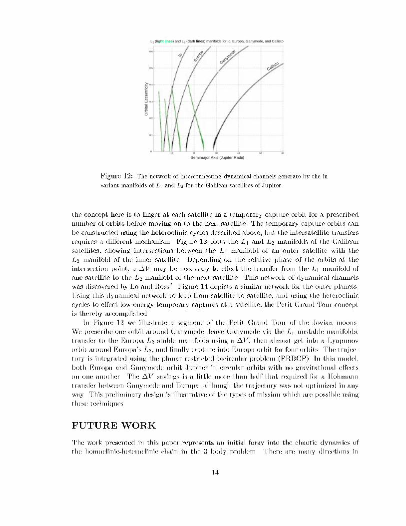
Figure 12: The network of interconnecting dynamical channels generate by the in-

variant manifolds of L1 and L2 for the Galilean satellites of Jupiter.

the concept here is to linger at each satellite in a temporary capture orbit for a prescribed

number of orbits before moving on to the next satellite. The temporary capture orbits can

be constructed using the heteroclinic cycles described above, but the intersatellite transfers

requires a di�erent mechanism. Figure 12 plots the L1 and L2 manifolds of the Galilean

satellites, showing intersections between the L1 manifold of an outer satellite with the

L2 manifold of the inner satellite. Depending on the relative phase of the orbits at the

intersection point, a �V may be necessary to e�ect the transfer from the L1 manifold of

one satellite to the L2 manifold of the next satellite. This network of dynamical channels

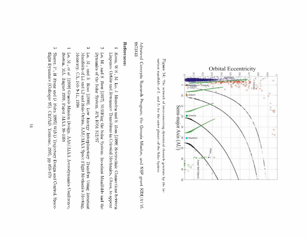
was discovered by Lo and Ross2. Figure 14 depicts a similar network for the outer planets.

Using this dynamical network to leap from satellite to satellite, and using the heteroclinic

cycles to e�ect low-energy temporary captures at a satellite, the Petit Grand Tour concept

is thereby accomplished.

In Figure 13 we illustrate a segment of the Petit Grand Tour of the Jovian moons.

We prescribe one orbit around Ganymede, leave Ganymede via the L1 unstable manifolds,

transfer to the Europa L2 stable manifolds using a �V , then almost get into a Lyapunov

orbit around Europa's L2, and �nally capture into Europa orbit for four orbits. The trajec-

tory is integrated using the planar restricted bicircular problem (PRBCP). In this model,

both Europa and Ganymede orbit Jupiter in circular orbits with no gravitational e�ects

on one another. The �V savings is a little more than half that required for a Hohmann

transfer between Ganymede and Europa, although the trajectory was not optimized in any

way. This preliminary design is illustrative of the types of mission which are possible using

these techniques.

FUTURE WORK

The work presented in this paper represents an initial foray into the chaotic dynamics of

the homoclinic-heteroclinic chain in the 3 body problem. There are many directions in

14

L2

Ganymede

L1

Jupiter

Jupiter

Europa’sorbit

Ganymede’sorbit

Transferorbit

∆V

L2

Europa

Jupiterx (Jupiter-Ganymede rotating frame)

y(Jupiter-G

anymed

erotatingfram

e)

x (Jupiter-Europa rotating frame)

y(Jupiter-E

uroparotatingfram

e)

x (Jupiter-centered inertial frame)

y(Jupiter-cen

teredinertial

fram

e)

Figure 13: (a) One orbit around Ganymede in rotating coordinates. (b) The transfer

from Ganymede to Europa via the invariant manifold intersections. (c) Temporary

capture by Europa into 4 orbits.

which this work may be continued. We mention a few of the most important problems and

applications in astrodynamics.

Extension of the 2-dimensional heteroclinic cycle to 3-dimension is the most important

problem for astrodynamic applications, since halo orbits and not Lyapunov orbits are the

ones of most interest to missions. The second problem is the systematic study of Earth-

return/collision orbits. The Genesis orbit, for example, is an Earth collision orbit not all

that di�erent from the spectacular Shoemaker-Levy 9 Jupiter collision orbit. The third

problem is the interaction of three-body trajectories with the Moon. Here we speak of

the interaction of the Sun-Earth Lagrange point dynamics with that of the Earth-Moon

Lagrange point dynamics. This interaction helped to provided the low energy capture

which rescued the Hitten mission (Belbruno and Miller 17). Similarly, the recent Hughes

geosychronous satellite rescue mission also used this dynamics. The fourth problem, a more

technical one, is to combine dynamical systems theory with optimal control methods. It

is hoped that the many di�culties which face optimal control problems may be alleviated

if the dynamics of the problems are taken more into consideration. For example, we are

currently working on targeting the stable manifold to compute an optimal transfer into

a halo orbit. Lastly, perhaps the most important problem in this �eld currently, is the

development of good software tools to perform the analysis. Work is continuing at JPL and

elsewhere to develop an integrated suite of software to more capably deal with the complex

dynamics of this most interesting region of space.

Acknowledgements: We thank Gerard G�omez and Josep Masdemont for many helpful

discussions and for sharing their wonderful software tools with us. We thank Paul Chodas

for discussions on the SL9 and NEO orbits. We also thank the following colleagues for

helpful discussions and comments: Brian Barden, Julia Bell, Peter Goldreich, Kathleen

Howell, �Angel Jorba, Andrew Lange, Jaume Llibre, Mart�inez, Richard McGehee, William

McLaughlin, Linda Petzold, Nicole Rappaport, Ralph Roncoli, Carles Sim�o, Scott Tremaine,

Stephen Wiggins, and Roby Wilson.

This work was carried out at the Jet Propulsion Laboratory and California Institute

of Technology under a contract with National Aeronautics and Space Administration. In

addtion, the work was partially supported by the Caltech President's fund, the NASA

15

Com

ets

Asteroids

Kuiper B

elt Objects

Pluto

Neptune

Uranus

Saturn

JupiterTrojans

0

0.1

0.2

0.3

0.4

0.5

0.6

0.7

0.8

0.9 1

Orbital Eccentricity

Sem

i-majo

rAxis(A

U)

2025

3035

1510

540

4550

Figure

14:Thenetw

ork

ofinterco

nnectin

gdynamica

lchannels

genera

tebythein-

varia

ntmanifo

ldsofL1andL2fortheouter

planets

oftheSolarSystem

.

Advanced

Concep

tsResea

rchProgram,theGenesis

Missio

n,andNSFgrantKDI/ATM-

9873133.

References:

1.Koon,W.S.,M.Lo,J.Marsd

enandS.Ross

[1999]Hetero

clinicConnectio

nsbetw

een

Liapunov

Orbits

andReso

nance

Transitio

nsin

Celestia

lMech

anics,

Chaos,to

appear.

2.Lo,M.,andS.Ross

[1997],SURFingtheSolarSystem

:Invaria

ntManifoldsandthe

Dynamics

oftheSolarSystem

,JPLIO

M312/97.

3.Lo,M.,andS.Ross

[1998],Low

Energ

yInterp

laneta

ryTransfers

Usin

gInvaria

nt

MnaifoldsofL1andL2andHaloOrbits,

AAS/AIA

ASpace

FlightMech

anics

Meetin

g,

Monterey,

CA,Feb

9-11,1998.

4.Lo,M.,etal.[1998]Genesis

Missio

nDesig

n,AAS/AIA

AAstro

dynamics

Conferen

ce,

Bosto

n,MA,August

1998,Paper

AIA

A98-4468.

5.Sharer,

P.,H.FranzandD.Folta

[1995]WIN

DTrajecto

ryDesig

nandContro

l,Space-

ightDynamics

(Collo

que95),CEPAD,Toulouse,

1995,pp.859-870.

16

6. Howell, K., D. Mains and B. Barden [1994] Transfer Trajectories from Earth Parking

Orbits to Sun-Earth Halo Orbits, AAS/AIAA Space ight Mechanics Meeting, Cocoa

Beach, FL, Feb. 14-16, 1994.

7. Wiggins, S. [1992] Chaotic Transport in Dynamical Systems, Springer Verlag, Berlin.

8. Meiss, J. [1992] Symplectic Maps, Variational Principles, and Transport, Review of

Modern Physics, Vol. 64, No. 3, July 1992.

9. Conley, C. [1968] Low Energy Transit Orbits in the Restricted Three-Body Problem,

SIAM J. Appl. Math. 16, 732-746.

10. McGehee, R. [1969] Some Homoclinic Orbits for the Restricted Three Body Problem,

Ph.D. Thesis, University of Wisconsin.

11. Llibre, J., R. Martinez and C. Sim�o [1985] Transversality of the Invariant Manifolds

Associated to the Lyapunov Family of Periodic Orbits Near L2 in the Restricted

Three-Body Problem, Journal of Di�erential Equations 58, 1985, 104-156.

12. Chodas, P. and D. Yeomans [1996] The Orbital Motion and Impact Circumstances of

Comet Shoemaker-Levy 9, in The Collision of Comet Shoemaker-Levy 9 and Jupiter,

edited by K.S. Noll, P.D. Feldman, and H.A. Weaver, Cambridge Unviersity Press,

1996.

13. Moser, J. [1973] Stable and Random Motions in Dynamical Systems with Special Em-

phasis on Celestial Mechanics, Princeton University Press.

14. Howell, K., B. Barden and M. Lo [1997] Application of Dynamical Systems Theory to

Trajectory Design for a Libration Point Mission, Journal of the Astronautical Sciences,

Vol. 45, No. 2, April-June 1997, pp. 161-178.

15. Bell, J., M. Lo and R. Wilson [1999] AAS/AIAA Astrodynamics Specialist Conference,

Girdwood Alaska, August 16-20, 1999.

16. Howell, K., B. Barden and M. Lo [1997] Trajectory Design Using a Dynamical Systems

Approach to GENESIS, AAS 97-709, AAS/AIAA Astrodynamics Specialist Confer-

ence, Sun Valley Idaho, August 4-7, 1997.

17. Belbruno, E. and J. Miller [1993] Sun-Perturbed Earth-to-Moon Transfers with Bal-

listic Capture, Journal of Guidance, Control and Dynamics 16, 770-775.

17