View Maintenance in a Warehousing Environment�

Yue Zhuge, Hector Garcia-Molina, Joachim Hammer, Jennifer Widom

Computer Science Department

Stanford University

Stanford, CA 94305-2140, USA

fzhuge,hector,joachim,widomg@cs.stanford.edu

Abstract

A warehouse is a repository of integrated information drawn from remote data sources.Since a warehouse e�ectively implements materialized views, we must maintain the views asthe data sources are updated. This view maintenance problem di�ers from the traditional onein that the view de�nition and the base data are now decoupled. We show that this decouplingcan result in anomalies if traditional algorithms are applied. We introduce a new algorithm,ECA (for \Eager Compensating Algorithm"), that eliminates the anomalies. ECA is basedon previous incremental view maintenance algorithms, but extra \compensating" queries areused to eliminate anomalies. We also introduce two streamlined versions of ECA for specialcases of views and updates, and we present an initial performance study that compares ECAto a view recomputation algorithm in terms of messages transmitted, data transferred, andI/O costs.

1 Introduction

Warehousing is an emerging technique for retrieval and integration of data from distributed,autonomous, possibly heterogeneous, information sources. A data warehouse is a repository ofintegrated information, available for queries and analysis (e.g., decision support, or data mining)[IK93]. As relevant information becomes available from a source, or when relevant information ismodi�ed, the information is extracted from the source, translated into a common model (e.g., therelational model), and integrated with existing data at the warehouse. Queries can be answeredand analysis can be performed quickly and e�ciently since the integrated information is directlyavailable at the warehouse, with di�erences already resolved.

1.1 The Problem

One can think of a data warehouse as de�ning and storing integrated materialized views overthe data from multiple, autonomous information sources. An important issue is the prompt andcorrect propagation of updates at the sources to the views at the warehouse. Numerous methodshave been developed for materialized view maintenance in conventional database systems; thesemethods are discussed in Section 2.

�This work was supported by ARPA Contract F33615-93-1-1339, by the Anderson Faculty Scholar Fund, by theCenter for Integrated Systems at Stanford University, and by equipment grants from Digital Equipment Corporationand IBM Corporation. The US Government is authorized to reproduce and distribute reprints for Governmentpurposes notwithstanding any copyright notation thereon. The views and conclusions contained in this documentare those of the authors and should not be interpreted as necessarily representing the o�cial policies or endorsements,either express or implied, of the US Government.

1

WarehouseSouce

Updates

Queries

Answers

Figure 1.1: Processing of updates in a single source model

Unfortunately, existing materialized view maintenance algorithms fail in a warehousing envi-ronment. Existing approaches assume that each source understands view management and knowsthe relevant view de�nitions. Thus, when an update occurs at a source, the source knows exactlywhat data is needed for updating the view.

However, in a warehousing environment, the sources can be legacy or unsophisticated systemsthat do not understand views. Sources can inform the warehouse when an update occurs, e.g., anew employee has been hired, or a patient has paid her bill. However, they cannot determine whatadditional data may or may not be necessary for incorporating the update into the warehouseviews. When the simple update information arrives at the warehouse, we may discover thatsome additional source data is necessary to update the views. Thus, the warehouse may have toissue queries to some of the sources, as illustrated in Figure 1.1. The queries are evaluated atthe sources later than the corresponding updates, so the source states may have changed. Thisdecoupling between the base data on the one hand (at the sources), and the view de�nition andview maintenance machinery on the other (at the warehouse), can lead the warehouse to computeincorrect views.

We illustrate the problems with three examples. For these examples, and for the rest ofthis paper, we use the relational model for data and relational algebra for views. Although weare using relational algebra, we assume that duplicates are retained in the materialized views.Duplicate retention (or at least a replication count) is essential if deletions are to be handledincrementally [BLT86, GMS93]. Note that the type of solution we propose here can be extendedto other data models and view speci�cation languages.

Also, in the examples and in this paper we focus on a single source, and a single view overseveral base relations. Our methods extend to multiple views directly. Handling a view that spansseveral sources requires the same type of solution, but introduces additional issues; see Section 7for a brief discussion.

Example 1: Correct View Maintenance

Suppose our source contains two base relations r1 and r2 as follows:

r1 :W X

1 2r2 :

X Y

2 4

Suppose the view at the warehouse is de�ned by the relational algebra expression:

V = �W (r1 ./ r2)

Initially the materialized view at the warehouse, MV, contains the single tuple [1]. Now supposetuple [2,3] is inserted into r2 at the source. For notation, we use insert(r; t) to denote the

2

insertion of tuple t into relation r (similarly for delete(r; t)), and we use ([t1]; [t2]; : : : ; [tn]) todenote a relation with tuples t1; t2; : : : ; tn. The following events occur:

1. Update U1 = insert(r2; [2; 3]) occurs at the source. Since the source does not know thedetails or contents of the view managed by the warehouse, it simply sends a noti�cation tothe warehouse that update U1 occurred.

2. The warehouse receives U1. Applying an incremental view maintenance algorithm, it sendsquery Q1 = �W (r1 ./ [2; 3]) to the source. (That is, the warehouse asks the source whichr1 tuples match with the new [2,3] tuple in r2.)

3. The source receives Q1 and evaluates it using the current base relations. It returns theanswer relation A1 = ([1]) to the warehouse.

4. The warehouse receives answer A1 and adds ([1]) to the materialized view, obtaining ([1],[1]).

In this example the �nal view at the warehouse is correct, i.e., it is equivalent to what one wouldobtain using a conventional view maintenance algorithm directly at the source.1 The next twoexamples show how the �nal view can be incorrect.

Example 2: A View Maintenance Anomaly

Assume we have the same relations as in Example 1, but initially r2 is empty:

r1 :W X

1 2r2 :

X Y

Consider the same view de�nition as in Example 1: V = �W (r1 ./ r2), and now suppose there aretwo consecutive updates: U1 = insert(r2; [2; 3]) and U2 = insert(r1; [4; 2]). The following eventsoccur. Note that initially MV = ;.

1. The source executes U1 = insert(r2; [2; 3]) and sends U1 to the warehouse.

2. The warehouse receives U1 and sends Q1 = �W (r1 ./ [2; 3]) to the source.

3. The source executes U2 = insert(r1; [4; 2]) and sends U2 to the warehouse.

4. The warehouse receives U2 and sends Q2 = �W ([4; 2] ./ r2) to the source.

5. The source receives Q1 and evaluates it on the current base relations: r1 = ([1; 2]; [4; 2]) andr2 = ([2; 3]). The resulting answer relation is A1 = ([1]; [4]), which is sent to the warehouse.

6. The warehouse receives A1 and updates the view to MV[ A1 = ([1]; [4]).

7. The source receives Q2 and evaluates it on the current base relations r1 and r2. The resultinganswer relation is A2 = ([4]), which is sent to the warehouse.

8. The warehouse receives answer A2 and updates the view to MV [A2 = ([1]; [4]; [4]).

1As stated earlier, for incremental handling of deletions we need to keep both [1] tuples in the view. For instance,if [2,4] is later deleted from r2, one (but not both) of the [1] tuples should be deleted from the view.

3

If the view had been maintained using a conventional algorithm directly at the source, thenit would be ([1]) after U1 and ([1],[4]) after U2. However, the warehouse �rst changes the view to([1],[4]) (in step 6) and to ([1],[4],[4]) (in step 8), which is an incorrect �nal state. The problemis that the query Q1 issued in step 4 is evaluated using a state of the base relations that di�ersfrom the state at the time of the update (U1) that caused Q1 to be issued. 2

We call the behavior exhibited by this example a distributed incremental view maintenance

anomaly, or anomaly for short. Anomalies occur when the warehouse attempts to update a viewwhile base data at the source is changing. Anomalies arise in a warehousing environment becauseof the decoupling between the information sources, which are updating the base data, and thewarehouse, which is performing the view update.

Example 3: Deletion Anomaly

Our third example shows that deletions can also cause anomalies. Consider source relations:

r1 :W X

1 2r2 :

X Y

2 3

Suppose that the view de�nition is V = �W;Y (r1 ./ r2). The following events occur. Note thatinitially MV = ([1; 3]).

1. The source executes U1 = delete(r1; [1; 2]) and noti�es the warehouse.

2. The warehouse receives U1 and emits Q1 = �W;Y ([1; 2] ./ r2).

3. The source executes U2 = delete(r2; [2; 3]) and noti�es the warehouse.

4. The warehouse receives U2 and emits Q2 = �W;Y (r1 ./ [2; 3]).

5. The source receives Q1. The answer it returns is A1 = ; since both relations are now empty.

6. The warehouse receives A1 and replaces the view by MV�A1 = ([1; 3]). (Di�erence is usedhere since the update to the base relation was a deletion [BLT86].)

7. Similarly, the source evaluates Q2, returns A2 = ;, and the warehouse replaces the view byMV� A2 = ([1; 3]).

This �nal view is incorrect: since r1 and r2 are empty, the view should be empty too. 2

1.2 Possible Solutions

There are a number of mechanisms for avoiding anomalies. As argued above, we are interestedonly in mechanisms where the source, which may be a legacy or unsophisticated system, does notperform any \view management." The source will only notify the warehouse of relevant updates,and answer queries asked by the warehouse. We also are not interested in, for example, solutionswhere the source must lock data while the warehouse updates its views, or in solutions wherethe source must maintain timestamps for its data in order to detect \stale" queries from thewarehouse. In the following potential solutions, view maintenance is autonomous from sourceupdating:

4

� Recompute the view (RV). The warehouse can either recompute the full view whenever anupdate occurs at the source, or it can recompute the view periodically. In Example 2, if thewarehouse sends a query to the source to recompute the view after it receives U2, then thesource will compute the answer relation A = ([1]; [4]) (assuming no further updates) andthe warehouse will correctly set MV = ([1]; [4]). Recomputing views is usually time andresource consuming, particularly in a distributed environment where a large amount of datamight need to be transferred from the source to the warehouse. In Section 6 we comparethe performance of our proposed solution to this one.

� Store at the warehouse copies of all relations involved in views (SC). In Example 2, supposethat the warehouse keeps up-to-date copies of r1 and r2. When U1 arrives, Q1 can beevaluated \locally," and no anomaly arises. The disadvantages of this approach are: (1)the warehouse needs to store copies of all base relations used in its views, and (2) copiedrelations at the warehouse need to be updated whenever an update occurs at the source.

� The Eager Compensating Algorithm (ECA). The solution we advocate avoids the overheadof recomputing the view or of storing copies of base relations. The basic idea is to add toqueries sent to the source compensating queries to o�set the e�ect of concurrent updates. Forinstance, in Example 2, consider the receipt of U2 = insert(r1; [4; 2]) in step 4. If we assumethat messages are delivered in order, and that the source handles requests atomically, thenwhen the warehouse receives U2 it can deduce that its previous query Q1 will be evaluatedin an \incorrect" state|Q1 will see the [4,2] tuple of the second insert. (Otherwise, thewarehouse would have received the answer to Q1 before it received the noti�cation of U2.)To compensate, the warehouse sends query:

Q2 = �W;Y ([4; 2] ./ r2)� �W;Y ([4; 2] ./ [2; 3])

The �rst part of Q2 is as before; the second part compensates for the extra tuple that Q1

will see. We call this an \eager" algorithm because the warehouse is compensating (in step4) even before the answer for Q1 has arrived (in step 6). In Section 5.2 we brie y discussa \lazy" version of this approach. Continuing with the example, we see that indeed theanswer received in step 6, A1 = ([1]; [4]), contains the extra tuple [4]. But, because of thecompensation, the A2 answer received in step 8 is empty, and the �nal view is correct.In Section 5.2 we present the Eager Compensating Algorithm in detail, showing how thecompensating queries are determined for an arbitrary view, and how query answers areintegrated into the view.

We also consider two improvements to the basic ECA algorithm:

� The ECA-Key Algorithm (ECAK). If a view includes a key from every base relation involvedin the view, then we can streamline the ECA algorithm in two ways: (1) Deletions can behandled at the warehouse without issuing a query to the source. (2) Insertions requirequeries to the source, but compensating queries are unnecessary. To illustrate point (1),consider Example 3, and suppose W and Y are keys for r1 and r2. When the warehousereceives U1 = delete(r1; [1; 2]) (step 1), it can immediately determine that all tuples of theform [1,x] are deleted from the view (where x denotes any value)|no query needs to be sentto the source. Similarly, U2 = delete[r2; [2; 3]] causes all [x,3] tuples to be deleted from theview, without querying the source. The �nal empty view is correct. Section 5.4 provides anexample illustrating point (2), and a description of ECAK . Note that ECAK does have the

5

disadvantage that it can only be used for a subset of all possible views|those that containkeys for all base relations.

� The ECA-Local Algorithm (ECAL). In ECAK , the warehouse processes deletes locally,without sending any queries to the source, but inserts still require queries to be sent to thesource. Generalizing this idea, for a given view de�nition and a given update, it is possibleto determine whether or not the update can be handled locally; see, e.g., [GB94, BLT86].ECAL combines local handling of updates with the compensation approach for maintenanceof arbitrary views.

1.3 Outline of Paper

In the next section we brie y review related research. Then, in Section 3, we provide a formalde�nition of correctness for view maintenance in a warehousing environment. As we will see,there are a variety of \levels" of correctness that may be of interest to di�erent applications. InSections 4 and 5 we present our new algorithms, along with a number of examples. In Section 6we compare the performance of our ECA algorithm to the view recomputation approach. InSection 7 we conclude and discuss future directions of our work. Additional details|additionalexamples, proofs, analyses, etc.|that are too lengthy and intricate to be included in the body ofthe paper are presented in Appendix A to Appendix D.

2 Related Research

Many incremental view maintenance algorithms have been developed. Most of them are designedfor a traditional, centralized database environment, where it is assumed that view maintenance isperformed by a system that has full control and knowledge of the view de�nition, the base rela-tions, the updated tuples, and the view [HD92, QW91, SI84]. These algorithms di�er somewhat inthe view de�nitions they handle. For example, [BLT86] considers select-project-join (SPJ) viewsonly, while algorithms in [GMS93] handle views de�ned by any SQL or Datalog expression. Somealgorithms depend on key information to deal with duplicate tuples [CW91], while others use acounting approach [GMS93].

A series of papers by Segev et al. studies materialized views in distributed systems [SF90,SF91, SP89a, SP89b]. All algorithms in these papers are based on timestamping the updatedtuples, and the algorithms assume there is only one base table. Other incremental algorithms,such as the \snapshot" procedure in [LHM+86], also assume timestamping and a single base table.In contrast, our algorithms have no restrictions on the number of base tables, and they requireno additional information. Note that although we describe our algorithms for SPJ views, ourapproach can be applied to adapt any existing centralized view maintenance algorithm to thewarehousing environment.

In both centralized and distributed systems, there are three general approaches to the timing ofview maintenance: immediate update [BLT86], which updates the view after each base relation isupdated, deferred update [RK86], which updates the view only when a query is issued against theview, and periodic update [LHM+86], which updates the view at periodic intervals. Performancestudies on these strategies have determined that the e�ciency of an approach depends heavily onthe structure of the base relations and on update patterns [Han87]. We assume immediate updatein this paper, but we observe that with little or no modi�cation our algorithms can be applied todeferred and periodic update as well.

6

3 Correctness

Our �rst task is to de�ne what correctness means in an environment where activity at the sourceis decoupled from the view at the warehouse. We start by de�ning the notion of events. In ourcontext, an event corresponds to a sequence of operations performed at the same site. There aretwo types of events at the source:

1. S up: the source executes an update U , then sends an update noti�cation to the warehouse.

2. S qu: the source evaluates a query Q using its current base relations, then sends the answerrelation A back to the warehouse.

There are two types of events at the warehouse:

1. W up: the warehouse receives an update U , generates a query Q, and sends Q to the sourcefor evaluation.

2. W ans: the warehouse receives the answer relation A for a query Q and updates the viewbased on A.

We will assume that events are atomic. That is, we assume there is a local concurrency controlmechanism (or only a single user) at each site to ensure that con icting operations do not overlap.With some extensions to our algorithms, this assumption could be relaxed. We also assume that,within an event, actions always follow the order described above. For example, within an eventS up, the source always executes the update operation �rst, then sends the update noti�cationto the warehouse.

We use e to denote an arbitrary event, se to denote a source event, and we to denote awarehouse event. Event types are subscripted to indicate a speci�c event, e.g., S upi, or W upj .For each event, relevant information about the event is denoted using a functional notation: Foran event e, query(e), update(e), and answer(e) denote respectively the query, update, and answerassociated with event e (when relevant). If event e is caused (\triggered") by another event, thentrigger(e) denotes the event that triggered e. For example, trigger(W upj) is an event of typeS up. The state of the data after an event e is denoted by state(e).

It is useful to immediately rule out algorithms that are trivially incorrect; for example, wherethe source does not propagate updates to the warehouse, or refuses to execute queries. These twoexamples are captured formally by the following rules:

� 8U = update(S upi): 9 W upj such that update(W upj) = U .

� 8Q = query(W upi): 9 S quj such that query(S quj) = Q.

There are a number of other obvious rules such as these that we omit for brevity.

Finally, we de�ne the binary event operator \<" to mean \occurs before". We assume thatmessages are delivered in order and are processed in order. In particular, let e1; e2; e3; e4 be fourevents. If trigger(e2) = e1, trigger(e4) = e3, and e1 and e3 occurred at the same site, thene1 < e3 i� e2 < e4. We also use the < relation to order states. That is, we say that si < sj ifstate(ei) = si, state(ej) = sj , and ei < ej .

7

3.1 Levels of Correctness

During the execution of a view maintenance algorithm, the system will process a sequence ofupdates U1; U2; : : : ; Un. In doing so, the source executes events se1; se2; : : :sep with correspondingresulting states ss1; ss2; : : : ; ssp. At the warehouse the triggered events are we1; we2; : : :weqwith corresponding resulting states ws1; ws2; : : : ; wsq. When we de�ne the notion of convergence(below), we consider executions that are �nite, i.e., that have a last update Un and last eventssep and wek. However, in general executions may be �nite or in�nite.

At the warehouse, the state of materialized view V after event wei is given by V [wsi], where Vis the view de�nition. Similarly, at the source, Q[ssi] is the result of evaluating query expressionQ on the relations existing after event sei. If we apply the view de�nition V to a source state,V [ssi], we get the state of the view had it been evaluated at the source after event sei.

An algorithm for warehouse view maintenance may exhibit the following properties:

� Convergence: For all �nite executions, V [wsq] = V [ssp]. That is, after the last update andafter all activity has ceased, the view is consistent with the relations at the source.

� Weak Consistency: For all executions and for all wsi, there exists an ssj such that V [wsi] =V [ssj ]. That is, every state of the view corresponds to some valid state of the relations atthe source.

� Consistency: For all executions and for every pair wsi < wsj , there exist ssk � ssl suchthat V [wsi] = V [ssk ] and V [wsj] = V [ssl]. That is, every state of the view corresponds toa valid source state, and in a corresponding order.

� Strong consistency: Consistency and convergence.

� Completeness: Strong consistency, and for each ssi there exists a wsj such that V [wsj ] =V [ssi]. That is, there is a complete order-preserving mapping between the states of the viewand the states of the source.

Although completeness is a nice property since it states that the view \tracks" the base dataexactly, we believe it is too strong a requirement and unnecessary in most practical warehousingscenarios. In some cases, convergence may be su�cient, i.e., knowing that \eventually" thewarehouse will have a valid state, even if it passes through intermediate states that are invalid.In other cases, consistency (weak or not) may be required, i.e., knowing that every warehousestate is valid with respect to some source state. Examples 2 and 3 showed that a straightforwardincremental view maintenance algorithm is not even weakly consistent in the environments weconsider. We will show that our Eager Compensating Algorithm is strongly consistent, and hencea satisfactory approach for most warehousing scenarios.

4 Views and Queries

Before presenting our algorithms, we must de�ne the warehouse views we handle and the typesof queries generated. In this paper, we consider views de�ned as:

V = �proj(�cond(r1 � r2 � : : :� rn))

where proj is a set of attribute names, cond is a boolean expression, and r1; : : : ; rn are baserelations. Note that any relational algebra expression constructed with select, project, and join

8

operations can be transformed into an equivalent expression of this form. For simplicity, we assumethat r1; : : : ; rn are distinct relations. Our algorithms can be extended to allowmultiple occurrencesof the same relation (e.g., by handling updates to such relations once for each appearance of therelation).

4.1 Signs

Our warehouse algorithms will handle two types of updates: insertions and deletions. (Modi�-cations must be treated as deletions followed by insertions, although extensions to our approachcould permit modi�cations to be treated directly.) For convenience, we adopt an approach similarto [BLT86] and use signs on tuples: + to denote an inserted or an existing tuple, and � to denotea deleted tuple. Tuple signs are propagated through relational operations, as we will illustrate.

Consider an update U1 = delete(r1; [1; 2]), which causes the warehouse to issue a query Q1 =�W ([1; 2] ./ r2). Using signs, we instead issue the query Q1 = �W (�[1; 2] ./ r2), where \�"attached to tuple [1,2] represents that this is a deleted tuple. Suppose that at the source there isan r2 tuple [2,3] (which by default has a + sign). The result of Q1, which we call A1, will containthe tuple �[1], i.e., the minus sign carries through. Relation A1 is then returned to the warehouse,where it is combined with the existing view by an operation (explained below): MV MV+A1.Because of the minus sign, the [1] tuple in A1 is removed from the view. Note that if the originalupdate U1 had been an insert, the tuple [1,2] would have a plus sign, and tuple [1] would insteadhave been added to the view. Using tuple signs allows us to handle inserts and deletes uniformlyand compactly in our algorithms.

More formally, existing tuples and inserted tuples always have a plus sign, while deleted tuplesalways have a minus sign. When a relational algebra expression operates on signed tuples, thesign of the result tuples is given by the following tables, where t, t1 and t2 are signed tuples:

t �cond(t) �proj(t)

+ + +� � �

t1 t2 t1 � t2+ + ++ � �� � +� + �

In addition, we de�ne two binary operators, also called + and �, which operate on relationswith signed tuples. For a relation r, let pos(r) denote the tuples with a plus sign and let neg(r)denote the tuples with a minus sign. Then:

r1 + r2 = (pos(r1) [ pos(r2))� (neg(r1)[ neg(r2))r1 � r2 = r1 + (�r2)

Operators + and � are commutative and associative, and they generalize to relational expressionsand to single tuples in the obvious way. The cross product � is distributive over + and �.

Note that the use of signed tuples is a notational convenience only|it is not necessary forsources to handle signed tuples in order to participate in our algorithms.

4.2 Query Expressions

In maintaining a view over relations r1; : : : ; rn, our algorithms will generate queries that containa collection of terms. Each term is of the form:

T = �proj(�cond(~r1 � ~r2 � : : :� ~rn)) (4.1)

9

where each ~ri is either a relation ri or an updated tuple ti of ri. A query is formed by a sum ofterms:

Q =Xi

Ti: (4.2)

As an example, the following relational algebra expression is query we might generate:

Q = �proj(�cond(r1 � [2; 3]� r3)) + �proj(�cond(�[1; 2]� [2; 3]� r3))

In our algorithms we often derive queries from earlier queries or from view de�nitions. Forexample, say we are given a view de�nition V = �proj(�cond(r1 � r2)), and we receive a deletionU = delete(r2; [3; 4]). Then the query we want to send to the source is V with r2 substituted by�[3; 4], i.e., Q = �proj(�cond(r1 � �[3; 4])). We use V hUi to denote view expression V with theupdated tuple of U substituted for U 's relation.

More formally, consider any query (or view de�nition) of the form Q =P

i Ti (recall Equa-tion 4.2). Let U be an update involving relation rk, and let tuple(U) be the updated tuple. ThenQhUi =

Pi TihUi, where for each Ti (recall Equation 4.1):

TihUi =

(; if ~rkis an updated tuple

�proj(�cond(~r1 � : : :� ~rk�1 � tuple(U)� ~rk+1 � : : :� ~rn)) if ~rkis relation rk

We also recursively de�ne QhU1; U2; : : :Uki = (QhU1; U2; : : :Uk�1i)hUki. That is, QhU1; U2 : : : ; Ukiis the query in which all updated relations have been replaced by the corresponding updatedtuples. Note that, by de�nition, if any two or more of the updates U1; U2; : : :Uk occur on thesame relation, then QhU1; U2; : : :Uki = ;.

5 The ECA Algorithm

In this section we present the details of our Eager Compensating Algorithm (ECA), introducedin Section 1 as a solution to the anomaly problem. ECA is an incremental view maintenancealgorithm based on the centralized view maintenance algorithm described in [BLT86]. ECAanticipates the anomalies that arise due to the decoupling between base relation updates andview modi�cation, and ECA compensates for the anomalies as needed to ensure correct viewmaintenance. Before we present ECA and its extensions, we �rst review the original incrementalview maintenance algorithm.

5.1 The Basic Algorithm

The view maintenance algorithm described in [BLT86] applies incremental changes to a view eachtime changes are made to relevant base relations. We adapt this algorithm to the warehousingenvironment and use our event-based notation:

Algorithm 5.1 (Incremental view maintenance algorithm)

At the source:

� S upi: execute Ui;send Ui to the warehouse;trigger event W upi at the warehouse

10

� S qui: receive query Qi;let Ai = Qi[ssi]; (ssi is the current source state)send Ai to the warehouse;trigger event W ansi at the warehouse

At the warehouse:

� W upi: receive update Ui;let Qi = V hUii;send Qi to the source;trigger event S qui at the source

� W ansi: receive Ai;update view: MV = MV+Ai

(end algorithm)

Notice that each update at the source triggers an S up event, which then triggers a W up eventat the warehouse, triggering an S qu event back at the source, and �nally a W ans event atthe warehouse (recall Figure 1.1). As shown in Examples 2 and 3, this algorithm may lead toanomalies. Consequently, using our de�nitions from Section 3, this basic algorithm is neitherconvergent nor weakly consistent in a warehousing environment.

5.2 The Eager Compensating Algorithm

We start by de�ning the set of \pending" queries at the warehouse:

De�nition: Consider the processing of an event we at the warehouse. Let the unanswered query

set for we, UQS(we), be the set of queries that were sent by the warehouse before we occurred,but whose answers were not yet received by we. We shorten UQS(we) to UQS when we refersto the event being processed. 2

When the warehouse receives an update Ui and UQS is not empty, then Ui may cause queriesQj in UQS to be evaluated incorrectly. The incorrectness arises because the queries Qj areassumed to be computed before Ui, but are actually computed after Ui. Thus, all queries in UQSwill \see" a source state that already re ects update Ui. ECA takes this behavior into account:When ECA issues its query in response to update Ui, ECA incorporates one \compensating query"for each query in UQS. The compensating queries o�set the e�ects of Ui on the results of queriesin UQS.

An important and subtle consequence of using compensating queries is that the results ofqueries should be applied to the view only after the answer to the last compensating query hasbeen received. If instead we updated the view after the receipt of each answer, then the viewmight temporarily assume an invalid state. (That is, in the terminology of Section 3.1, thealgorithm would be convergent but not consistent.) To avoid invalid view states, ECA collectsall intermediate answers in a temporary relation called COLLECT, and only updates the view whenthe last answer has been received (i.e. when UQS = ;).

Algorithm 5.2 (ECA)

COLLECT = ;.The source events behave exactly as in Algorithm 5.1. At the warehouse:

11

� W upi: receive Ui;let Qi = V hUii �

PQj2UQS

QjhUii

send Qi to the source;trigger event S qui at the source

� W ansi: receive Ai;let COLLECT = COLLECT + Ai;if UQS = ;then f MV MV+ COLLECT; COLLECT ; gelse do nothing

(end algorithm)

5.3 Example

The following example illustrates ECA handling three insertions to three di�erent base relations.A number of additional ECA examples are given in Appendix A.

Example 4: ECA

Consider source relations:

r1 :W X

1 2r2 :

X Yr3 :

X Y

Let the view de�nition be V = �W (r1 ./ r2 ./ r3), and suppose the following events occur.Initially, the materialized view at the warehouse is empty, and COLLECT is initialized to empty.For brevity, we omit the source events, only listing events occurring at the warehouse. We assumethat the three updates occur at the source before any queries are answered.

1. Warehouse receives U1 = insert(r1; [4; 2])

Warehouse sends Q1 = V hU1i = �W ([4; 2] ./ r2 ./ r3)

2. Warehouse receives U2 = insert(r3; [5; 3])

UQS = fQ1g

Warehouse sends Q2 = V hU2i �Q1hU2i= �W (r1 ./ r2 ./ [5; 3])� �W ([4; 2] ./ r2 ./ [5; 3])

3. Warehouse receives U3 = insert(r2; [2; 5])

UQS = fQ1; Q2g

Warehouse sends Q3 = V hU3i �Q1hU3i �Q2hU3i= �W (r1 ./ [2; 5] ./ r3)� �W ([4; 2] ./ [2; 5] ./ r3)� �W ((r1� [4; 2]) ./ [2; 5] ./ [5; 3])

4. Warehouse receives A1 = [4]

COLLECT = ([4]), UQS = fQ2; Q3g

12

5. Warehouse receives A2 = [1]

COLLECT = ([1],[4]), UQS = fQ3g

6. Warehouse receives A3 = ;

COLLECT = ([1],[4]), UQS = ;

Warehouse updates view: MV = ;+ COLLECT = ([1]; [4]), which is correct. 2

A complete proof showing that the algorithm is strongly consistent is given in Appendix B.Notice, however, that ECA is not complete. Recalling Section 3.1, completeness requires thatevery source state be re ected in some view state. Clearly some source states may be \missed"by the ECA algorithm while it collects query answers. We can modify ECA to obtain a completealgorithm that we call the Lazy Compensating Algorithm (LCA). For each source update, LCAwaits until it has received all query answers (including compensation) for the update, then appliesthe changes for that update to the view. A detailed description of LCA is beyond the scope ofthis paper. LCA is less e�cient than ECA, and we believe that strong consistency is su�cient formost environments and completeness is generally not needed. Hence, we expect that ECA willbe more useful than LCA in practice.

5.4 The ECA-Key Algorithm

We can \streamline" ECA in the case where key attributes for each base relation are present inthe view. (In fact, it could be advisable to design warehouse view de�nitions with this propertyin mind, for more e�cient maintenance.) The ECA-Key Algorithm (ECAK) proceeds as follows:

1. COLLECT is initialized with the current materialized view (not the empty set). Instead ofstoring modi�cations to MV, COLLECT is a \working copy" of MV.

2. When a delete is received at the warehouse, no query is sent to the source. Instead, thedelete is applied to COLLECT immediately, using a special key-delete operation de�ned below.

3. When an insert is received at the warehouse, a query is sent to the source. However, nocompensating queries are added. Thus, when an insert U is received, the query sent to thesource is simply V hUi.

4. As answers are received, they are accumulated in the COLLECT set, as in the original ECA.However, duplicate tuples are not added to the COLLECT set. When the view contains keysfor all base relations, there can be no duplicates in the view. Thus, if a duplicate occurs, itis due to an anomaly and can be ignored.

5. If UQS is empty, the materialized view is updated, replacing it with the tuples in COLLECT.

Example 5: ECAK

Consider the following source relations, where W and Y are key attributes.

r1 :W X

1 2r2 :

X Y

2 3

Suppose that the warehouse view de�nition is V = �W;Y (r1 ./ r2), and the following events occur.Initially, the materialized view at the warehouse is MV = ([1,3]), and COLLECT = MV.

13

1. U1 = insert(r2; [2; 4])

Warehouse sends Q1 = V hU1i = �W;Y (r1 ./ [2; 4])

2. U2 = insert(r1; [3; 2])

Warehouse sends Q2 = V hU2i = �W;Y ([3; 2] ./ r2)

3. U3 = delete(r1; [1; 2])

Operation key-delete(V, r1, [1,2]) (see below) deletes tuples of the form [1,x], obtainingCOLLECT = COLLECT � ([1,3]) = ;, UQS = fQ1; Q2g

4. Warehouse receives A1 = ([3; 4])

COLLECT = COLLECT + ([3,4]) = ([3,4]), UQS = fQ2g

5. Warehouse receives A2 = ([3; 3]; [3; 4])

First, A2 is added to COLLECT: duplicate tuple [3,4] is not added, so COLLECT = ([3,3],[3,4]).Next, since UQS = ;, MV is set to COLLECT, so MV = ([3,3],[3,4]). Note that COLLECT isnot reset to empty.

The special operation key-delete(MV, r1, [1,2]) deletes from MV all tuples whose attribute corre-sponding to r1's key (i.e., attribute W ) is equal to the key value in tuple [1,2] (i.e., 1).

Observe that if we had installed COLLECT intoMV in steps 3 or 4, without waiting for UQS =;, then the view would have temporarily assumed an invalid state (resulting in convergence butnot consistency).

It is the presence of keys in the view de�nition that makes it possible to perform deletes at thewarehouse without issuing queries to the source, and that eliminates the need for compensatingqueries in the case of inserts. Consider deletions �rst. Since each view tuple contains key valuesfor all base relations, when a base relation tuple t is deleted, we can use the key values in t toidentify which tuples in the view were derived using t. These are the view tuples that must bedeleted.

Now consider insertions. Since insertions cause queries to be sent to the source, anomalies canstill arise. However, all such anomalies result in either duplicate view tuples (which we can detectand ignore), or missing tuples that would have been deleted anyway. As illustration, suppose Q1

of Example 5 had been executed when U1 occurred; it would have evaluated to ([1,4]). Instead,because of the delay, we have A1 = ([3,4]). A1 is incorrect in two ways: (1) It contains an extratuple [3,4] produced because Q1 was evaluated after insert U2. (2) It is missing tuple [1,4] becauseQ1 was evaluated after delete U3. However, both of these problems are resolved at the warehouse:(1) The extra tuple [3,4] is identi�ed as a duplicate when A2 is received. (2) The missing tuple[1,4] would have been deleted by U3. Details and a sketch for the ECAK correctness proof appearin Appendix C.

5.5 The ECA-Local Algorithm

The original ECA uses compensating queries to avoid the anomalies that may occur when queriesare sent to the source. ECAK relies on key properties to avoid compensating queries; furthermore,ECAK introduces the concept of local updates (deletions, in the case of ECAK), which can behandled at the warehouse without sending queries to the source. The last algorithm we discuss,

14

the ECA-Local Algorithm (ECAL) combines the compensating queries of ECA with the localupdates of ECAK to produce a streamlined algorithm that applies to general views.

In ECAL, each update is handled either locally or non-locally. A number of papers, e.g.,[BLT86, GB94, TB88], describe conditions when, for a particular view de�nition and a particularbase relation update, the view can be updated without further access to base relations (i.e., theview is autonomously computable, using the terminology of [BLT86]). These results can be used toidentify which updates ECAL will process locally. For updates that cannot be processed locally,ECA is used (assuming the key condition for ECAK does not hold), with compensating querieswhenever necessary.

Unfortunately, maintaining the correct order of execution among local and non-local processingin ECAL is not straightforward. Intuitively, we can process a local update as soon as all queries forprevious updates have been answered and applied to the view. However, consider three updates,U1, U2, and U3, where U2 is the only local update. Suppose we process U2 as soon as the query Q1

for U1 is answered. Since ECAL uses compensating queries, the \true" view update corresponding

to U1 may include not only the answer for Q1, but also compensations appearing in queries forlater updates (such as U3). To correctly handle this scenario, ECAL must bu�er updates and,in some cases, \split" query results (separating compensation from original), in order to processlocal updates on a correct version of the view. The details of ECAL, and determining whetherthe additional overhead is worthwhile, is left as future work.

5.6 Properties of the ECA family

ECA, and its extensions ECAK and ECAL, have the following desirable properties:

1. They are incremental, meaning that they update the warehouse based on updates to thesource, rather than recomputing the complete warehouse view from scratch.

2. They do not place any additional burden on the sources (e.g., timestamps, locks, etc.).

3. When the update frequency is low, i.e. when the answer to a warehouse query comes backbefore the next update occurs at the source, then the ECA algorithms behave exactly likethe original incremental view maintenance algorithm. (Compensating queries are used onlywhen the answer to a query has not been received before the next update occurs at thesource.)

6 Performance Evaluation

In Section 1.2 we outlined several strategies for view maintenance in a warehousing environment:recomputing the view (RV), storing copies of all base relations (SC), our Eager CompensatingAlgorithm (ECA), and our extensions ECA-Key (ECAK) and ECA-Local (ECAL). All of theseapproaches provide strong consistency (recall Section 3.1). Thus, a natural issue to explore isthe relative performance of these strategies. In this paper we evaluate only the basic algorithms,RV and ECA. From the performance perspective, ECAK is simply an enhancement to ECA thateliminates querying the source in certain cases. Since there is very little additional overheadin ECAK , ECAK should certainly be used when it is possible to arrange for warehouse views toinclude all base relation keys. Storing copies of base relations (SC) can be seen as an enhancementto any of our algorithms, requiring an \orthogonal" performance comparison (based on warehouse

15

storage costs, etc.) that is beyond the scope of this paper. As discussed in Section 5.5, ECAL

requires complex processing at the warehouse, the measurement of which falls outside the scopeof our performance evaluation. We plan to address performance issues for SC and ECAL, alongwith a more extensive evaluation of ECA, as future work.

When we intuitively compare RV and ECA, it seems that ECA should certainly outperformRV, since ECA is an incremental update algorithm while RV recomputes the view from scratch.However, ECA may need to send many more queries to the source than RV. In addition, ECA'squeries grow in complexity as compensations upon compensations are added. Hence, we seekto determine when it is more e�ective to recompute the entire view, rather than maintaining itincrementally with the associated extra activity.

To answer this question, we provide an initial performance analysis of RV and ECA. We notethat this is not a comprehensive analysis, as there are a number of parameters we have not fullystudied (ranging from the number of relations, to the exact sequence and timing of the updates,to the way queries are optimized at the source). Rather, we have selected a \representative"scenario that serves to illustrate the performance tradeo�s.

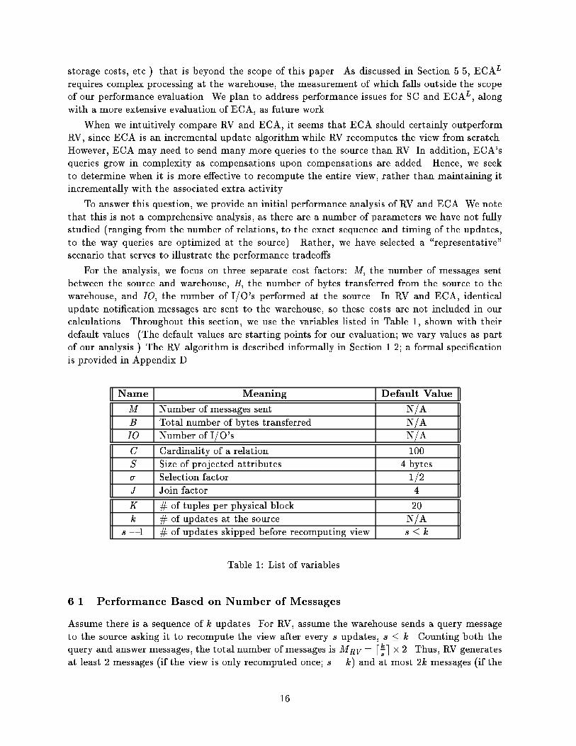
For the analysis, we focus on three separate cost factors: M, the number of messages sentbetween the source and warehouse, B, the number of bytes transferred from the source to thewarehouse, and IO, the number of I/O's performed at the source. In RV and ECA, identicalupdate noti�cation messages are sent to the warehouse, so these costs are not included in ourcalculations. Throughout this section, we use the variables listed in Table 1, shown with theirdefault values. (The default values are starting points for our evaluation; we vary values as partof our analysis.) The RV algorithm is described informally in Section 1.2; a formal speci�cationis provided in Appendix D.

Name Meaning Default Value

M Number of messages sent N/A

B Total number of bytes transferred N/A

IO Number of I/O's N/A

C Cardinality of a relation 100

S Size of projected attributes 4 bytes

� Selection factor 1/2

J Join factor 4

K # of tuples per physical block 20

k # of updates at the source N/A

s � 1 # of updates skipped before recomputing view s � k

Table 1: List of variables.

6.1 Performance Based on Number of Messages

Assume there is a sequence of k updates. For RV, assume the warehouse sends a query messageto the source asking it to recompute the view after every s updates, s � k. Counting both thequery and answer messages, the total number of messages isMRV = dk

se� 2. Thus, RV generates

at least 2 messages (if the view is only recomputed once; s = k) and at most 2k messages (if the

16

view is recomputed after every update; s = 1). For ECA, if there are k updates, we always havek queries and k answers, so there are 2k messages.2

Thus, in the situation least favorable for ECA, ECA sends 2k messages while RV sends 2messages. Of course, the price of the RV approach in this case is that the state of the warehouseview lags well behind the state of the base relations. In the most favorable situation for ECA,ECA and RV both send 2k messages.

6.2 Performance Based on Data Transferred

To analyze the number of bytes transferred (and later on the number of I/O's), we introduce asample scenario consisting of a particular view and a particular sequence of update operations.As mentioned earlier, we have chosen to focus on a sample scenario to illustrate the performancetradeo�s while keeping the number of parameters manageable.

Example 6: Example warehouse scenario

Base relation schema: r1(W;X), r2(X; Y ), r3(Y; Z)

View de�nition: V = �W;Z(�cond(r1 ./ r2 ./ r3))

Updates: U1 = insert[r1, t1], U2 = insert[r2, t2], U3 = insert[r3, t3] 2

The condition cond involves a comparison between attributes W and Z (e.g., W > Z). (Thiscondition has an impact on the derivation of the the number of I/O's performed.) Later we extendthis example to a sequence of k updates.

We make the following assumptions in our analysis:

1. The cardinality (number of tuples) of each relation is some constant C.

2. The size of the combined W , Z attributes is S bytes.

3. The join factor J(ri; a) is the expected number of tuples in ri that have a particular valuefor attribute a. We assume that the join factor is a constant J in all cases. So, for example,if we join a 20-tuple relation with a second relation, we expect to get 20J tuples.

4. The selectivity for the condition cond is given by �, 0 � � � 1.

5. We assume that C, J and our other parameters do not change as updates occur. Thisclosely approximates their behavior in practice when the updates are single-tuple insertsand deletes (so the size and selectivity do not change signi�cantly), or when C and J are solarge that the e�ect of updates is insigni�cant.

Not surprisingly, for RV the fewest bytes are transferred (BRVBest) when the view is recom-puted only once, after U3 has occurred. The worst case (BRVWorst) is when the view is recom-puted after each update. For ECA, the best case (BECABest) is when no compensating queriesare needed, i.e., the updates are su�ciently spaced so that each query is processed before the next

2Because ECA uses signed queries (recall Section 4.1), and some sources|such as an SQL server|may need tohandle the positive and negative parts of such queries separately, we may need to send a pair of queries for someupdates instead of a single query. We assume the pair of queries is \packaged" as one message, and the pair ofanswers also is returned in a single message.

17

0

200

400

600

800

0 5 10 15 20

B

C

BRVBestBRVWorst

BECABestBECAWorst

Figure 6.2: B versus C

0

2000

4000

6000

8000

10000

12000

0 30 60 90 120

B

k

BRVBestBRVWorst

BECABestBECAWorst

Figure 6.3: B versus k

update occurs at the source. Note that in this case, ECA performs as e�ciently as the originalincremental algorithm (Algorithm 5.1). The worst case for ECA (BECAWorst) is when all updatesoccur before the �rst query arrives at the source. Intuitively, the di�erence between the best andworst cases of ECA represents the \compensation cost."

The calculations for analyzing our algorithms are rather complex and therefore omitted here;the complete derivations can be found in Appendix D. In particular, the expressions derived inAppendix D for the number of bytes transferred are:

BRVBest = S�CJ2

BRVWorst = 3S�CJ2

BECABest = 3S�J2

BECAWorst = 3S�J(J + 1)

Figure 6.2 shows the number B of bytes transferred as a function of the cardinality C. (Inall of our graphs, parameters have the default values of Table 1 unless otherwise indicated.) Bestand worst cases are shown for both algorithms. Thus, for each algorithm, actual performancewill be somewhere in between the best and worst case curves, depending on the timing of updatearrivals (for ECA) and the frequency of view recomputation (for RV).

From Figure 6.2 we see that in spite of the compensating queries, ECA is much more e�cientthan RV (in terms of data transferred), unless the relations involved are extremely small (lessthan approximately 5 tuples each). This result continues to hold over wide ranges of the joinselectivity J , except if J is very small (see equations above).

One of the reasons ECA appears to perform so well is that we are considering only threeupdates, so the amount of \compensation work" is limited. In Appendix D we extend our analysisto an arbitrary number k of updates and obtain the following equations:

BRVBest = S�CJ2

BRVWorst = kS�CJ2

BECABest = kS�J2

BECAWorst = kS�J2 + k(k � 1)S�J=3

Figure 6.3 shows the number of bytes transferred as a function of k when C = 100. As expected,there is a crossover point beyond which recomputing the view once (RV's best case) is superior

18

to even the best case for ECA. For our example, this crossover is at 100 updates. In the ECAworst case, when all updates occur at the source before any of the warehouse queries arrive,each warehouse query must compensate every preceding update. This behavior results in ECAtransmitting additional data that is quadratic on the number of updates. Hence, in the situationleast favorable for ECA, RV outperforms ECA when 30 or more updates are involved. Bear inmind that this situation occurs only if all updates precede all queries. If updates and queries areinterleaved at the source, then performance will be somewhere between the ECA best and worstcases, and the crossover point will be somewhere between 30 and 100 updates.

Also notice that Figure 6.3 is for relatively small relations (C = 100); for larger cardinalitiesthe crossover points will be at larger number of updates. Finally, note that the RV best case wehave been comparing against assumes the view is recomputed once, no matter how many updatesoccur. If RV recomputes the view more frequently (such as once per some number of updates),then its cost will be substantially higher. In particular, BRVWorst is very expensive and alwayssubstantially worst than BECAWorst.

6.3 Performance Based on I/O

We continue using Example 6 and now estimate the number of I/O's performed at the source.We consider two extreme scenarios. In the �rst scenario, indexing is used and ample memory isavailable, while in the second scenario memory is very limited and there are no indexes. Studyingthese extremes lets us discover the conditions that are most favorable for the algorithms weconsider.

For our analysis we do not consider optimization across query terms or the e�ects of caching:If a query consists of several terms (recall De�nition 4.2), each one is evaluated independently.Furthermore, if in evaluating a term we need a particular page that was accessed in evaluatingthe previous term, we still assume that the page has to be read from disk (as opposed to a cache).Since only ECA uses multi-term queries, our results for ECA will be pessimistic. (Our no-cachingassumption could potentially hurt RV as well, but only in the case where recomputations arefrequent enough that pages from previous evaluations are still in memory.)

For the �rst scenario (call it Scenario 1) we assume that main memory is large enough tohold the parts of all three relations that participate in the join. We also assume that there areclustering indexes on X for r1 and r2, a clustering index on Y for r3, and a non-clustering indexon Y for r2. These indexes reside in memory and their access generates no I/O.

In Appendix D we derive the following equations for the number of I/O's in Scenario 1:

IORVBest = 3IIORVWorst = 9IIOECABest = 3min(I; J) + 3IOECAWorst = 3min(I; J) + 6

where I = dC=Ke is the number of I/O's needed to read an entire base relation. From theseequations we can see that in the situation least favorable for ECA, ECA is at most a constantfactor of 6 I/O's more expensive than RV. However, if J < I , then ECA can outperform RVarbitrarily (bounded by I�J). For large relations, we would expect J to be substantially smallerthan I , in which case even ECA's worst case will have substantially fewer I/O's than RV.

For the second I/O scenario (Scenario 2) we assume that there are no indexes, and thatthere are only three free memory blocks to be used for nested-loop join processing. The relevant

19

equations, derived in Appendix D, are:

IORVBest = I3

IORVWorst = 3I3

IOECABest = 3II 0

IOECAWorst = 3I(I 0 + 1)

where I = dC=Ke and I 0 = dC=(2K)e. It is apparent from these equations that, as expected, theI/O costs for this scenario are much higher than for Scenario 1. However, the di�erence betweenECA and RV is even more dramatic now. Unless the relations are very small (occupying less than3 blocks), even in the situation least favorable for ECA, ECA outperforms RV by a factor of I .

As with our evaluation of the amount of data transferred, the performance of ECA bene�tsfrom the fact that we have been considering only three updates. Hence, we extend both scenariosto the case of k updates. The equations, again derived in Appendix D, follow. For brevity, weconsider here only the (likely) case in which J < I :

Scenario 1:

IORVBest = 3IIORVWorst = 3kIIOECABest = k(J + 1)IOECAWorst = k(J + 1) + k(k � 1)=3

Scenario 2:

IORVBest = I3

IORVWorst = kI3

IOECABest = kII 0

IOECAWorst = kII 0 + Ik(k� 1)=3

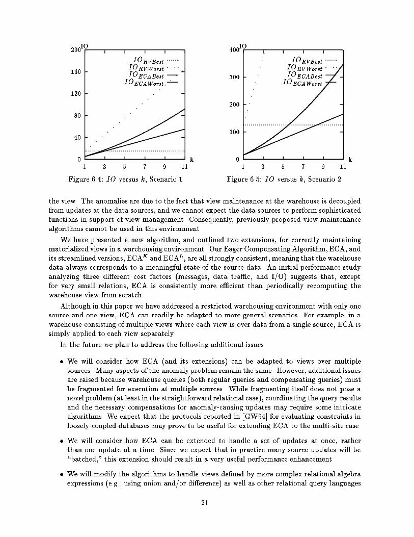
Figures 6.4 and 6.5 show the results when J = 4 and C = 100 (and hence I = 5). The shapeof these curves is similar to those in Figure 6.3, and thus our conclusions for I/O costs are similarto those for data transmission. The main di�erence is that the crossover points occur with smallerupdate sequences: k = 3 for Scenario 1, and 5 < k < 8 for Scenario 2, as opposed to a crossoverbetween k = 30 and k = 100 when data transfer is the metric. Intuitively, this means that ECAis not as e�ective at reducing I/O costs as it is at reducing data transfer. However, ECA canstill reduce I/O costs over RV signi�cantly, especially if relations are larger than the 100 tuplesconsidered for these �gures. Also, we expect that the I/O performance of ECA would improve ifwe incorporated multiple term optimization or caching into the analysis.

As a �nal note, we remind the reader that our results are for a particular three-relation view.In spite of this, we believe that our results are indicative of the performance issues faced inchoosing between RV and ECA. Our results indicate that when the view involves more relations,ECA should still generally outperform RV.

7 Conclusion

Data warehousing is an emerging (and already very popular) technique used in many applicationsfor retrieval and integration of data from autonomous information sources. However, warehousingtypically is implemented in an ad-hoc way. We have shown that standard algorithms for maintain-ing a materialized view at a warehouse can lead to anomalies and inconsistent modi�cations to

20

0

40

80

120

160

200

1 3 5 7 9 11

IO

k

IORVBestIORVWorst

IOECABestIOECAWorst

Figure 6.4: IO versus k, Scenario 1

0

100

200

300

400

1 3 5 7 9 11

IO

k

IORVBestIORVWorst

IOECABestIOECAWorst

Figure 6.5: IO versus k, Scenario 2

the view. The anomalies are due to the fact that view maintenance at the warehouse is decoupledfrom updates at the data sources, and we cannot expect the data sources to perform sophisticatedfunctions in support of view management. Consequently, previously proposed view maintenancealgorithms cannot be used in this environment.

We have presented a new algorithm, and outlined two extensions, for correctly maintainingmaterialized views in a warehousing environment. Our Eager Compensating Algorithm, ECA, andits streamlined versions, ECAK and ECAL, are all strongly consistent, meaning that the warehousedata always corresponds to a meaningful state of the source data. An initial performance studyanalyzing three di�erent cost factors (messages, data tra�c, and I/O) suggests that, exceptfor very small relations, ECA is consistently more e�cient than periodically recomputing thewarehouse view from scratch.

Although in this paper we have addressed a restricted warehousing environment with only onesource and one view, ECA can readily be adapted to more general scenarios. For example, in awarehouse consisting of multiple views where each view is over data from a single source, ECA issimply applied to each view separately.

In the future we plan to address the following additional issues.

� We will consider how ECA (and its extensions) can be adapted to views over multiplesources. Many aspects of the anomaly problem remain the same. However, additional issuesare raised because warehouse queries (both regular queries and compensating queries) mustbe fragmented for execution at multiple sources. While fragmenting itself does not pose anovel problem (at least in the straightforward relational case), coordinating the query resultsand the necessary compensations for anomaly-causing updates may require some intricatealgorithms. We expect that the protocols reported in [GW94] for evaluating constraints inloosely-coupled databases may prove to be useful for extending ECA to the multi-site case.

� We will consider how ECA can be extended to handle a set of updates at once, ratherthan one update at a time. Since we expect that in practice many source updates will be\batched," this extension should result in a very useful performance enhancement.

� We will modify the algorithms to handle views de�ned by more complex relational algebraexpressions (e.g., using union and/or di�erence) as well as other relational query languages

21

(e.g., SQL or Datalog).

� We will explore how the algorithms can be adapted to other data models (e.g., an object-based data model).

References

[BLT86] J.A. Blakeley, P.-A. Larson, and F.W. Tompa. E�ciently updating materialized views. InProceedings of the ACM SIGMOD International Conference on Management of Data, pages61{71, Washington, D.C., June 1986.

[CW91] S. Ceri and J. Widom. Deriving production rules for incremental view maintenance. InProceedings of the Seventeenth International Conference on Very Large Data Bases, pages577{589, Barcelona, Spain, September 1991.

[GB94] Ashish Gupta and J. A. Blakeley. Updating materialized views using the view contents andthe update. In unpublished document, 1994.

[GMS93] A. Gupta, I. Mumick, and V. Subrahmanian. Maintaining views incrementally. In Preceedingsof the 1993 ACM SIGMOD International Conference on Management of Data, pages 157{166, Washington, D.C., May 1993.

[GW94] P. Grefen and J. Widom. Integrity constraint checking in federated databases. Submittedfor publication, 1994.

[Han87] E.N. Hanson. A performance analysis of view materialization strategies. In Proceedings ofthe ACM SIGMOD International Conference on Management of Data, pages 440{453, 1987.

[HD92] J.V. Harrison and S.W. Dietrich. Maintenance of materialized views in a deductive database:An update propagation approach. In Proceedings of the 1992 JICLSP Workshop on DeductiveDatabases, pages 56{65, 1992.

[IK93] W.H. Inmon and C. Kelley. Rdb/VMS: Developing the Data Warehouse. QED PublishingGroup, Boston, London, Toronto, 1993.

[LHM+86] B. Lindsay, L.M. Haas, C. Mohan, H. Pirahesh, and P. Wilms. A snapshot di�erential refreshalgorithm. In Proceedings of the ACM SIGMOD International Conference on Managementof Data, Washington, D.C., May 1986.

[QW91] X. Qian and G. Wiederhold. Incremental recomputation of active relational expressions.IEEE Transactions on Knowledge and Data Engineering, 3(3):337{341, September 1991.

[RK86] N. Roussopoulos and H. Kang. Preliminary design of ADMS+-: A workstation-mainframeintegrated architecture for database management systems. In Proceedings of the TwelfthInternational Conference on Very Large Data Bases, pages 355{364, Kyoto, Japan, August1986.

[SF90] A. Segev and W. Fang. Currency-based updates to distributed materialized views. In Pro-ceedings of the Sixth International Conference on Data Engineering, pages 512{520, LosAlamitos, February 1990.

[SF91] A. Segev and W. Fang. Optimal update policies for distributed materialized views. Man-agement Science, 37(7):851{70, July 1991.

[SI84] O. Shmueli and A. Itai. Maintenance of views. In Proceedings of the ACM SIGMOD Inter-national Conference on Management of Data, pages 240{255, Boston, Massachusetts, May1984.

[SP89a] A. Segev and J. Park. Maintaining materialized views in distributed databases. In Proceed-ings of the Fifth International Conference on Data Engineering, pages 262{70, Los Angeles,February 1989.

22

[SP89b] A. Segev and J. Park. Updating distributed materialized views. IEEE Transactions onKnowledge and Data Engineering, 1(2):173{184, June 1989.

[TB88] F.WM. Tompa and J.A. Blakeley. Maintaining materialized views without accessing basedata. Information Systems, 13(4):393{406, 1988.

[ZGMHW94] Y. Zhuge, H. Garcia-Molina, J. Hammer, and J. Widom. View maintenance in a warehousingenvironment. Technical report, Stanford University, October 1994. Available via anonymousftp from host db.stanford.edu as pub/zhuge/1994/anomaly-full.ps.

23

A Examples of ECA Applications

The following three scenarios are additional examples of ECA applications in a warehousingenvironment.

Example 7: Insertion

This example has the same base relations and source updates as in Example 4, but the eventorder is di�erent:

r1 :W X

1 2r2 :

X Yr3 :

X Y

The view is de�ned to be V = �W (r1 ./ r2 ./ r3) as in Example 4, and is empty originally.

1. Warehouse receives U1 = insert(r1; [4; 2]);

Warehouse sends Q1 = V hU1i = �W ([4; 2] ./ r2 ./ r3).

2. Warehouse receives U2 = insert(r3; [5; 3]); Now UQS = fQ1g

Warehouse sends Q2 = V hU2i �Q1hU2i = �W (r1 ./ r2 ./ [5; 3])��W ([4; 2] ./ r2 ./ [5; 3])

3. Warehouse receives A1 = ;, COLLECT = ;, UQS = fQ2g

4. Warehouse receives U3= insert(r2; [2; 5]); UQS = fQ2g. Warehouse sends

Q3 = V hU3i � Q2hU3i

= �W (r1 ./ [2; 5] ./ r3)��W (r1 ./ [2; 5] ./ [5; 3])+ �W ([4; 2] ./ [2; 5] ./ [5; 3])

5. Warehouse receives A2 = [1], COLLECT = ([1]), UQS = fQ3g.

6. Warehouse receives A3 = [4], COLLECT = ([1],[4]), UQS = ;. The view is updated to be:MV = ;+ COLLECT = ([1]; [4]),

2

Example 8: Deletion

Base relations:

r1

W X

1 24 2

r2X Y

2 3

The view is de�ned to be V = �W (r1 ./ r2). It contains two tuples ([1], [4]) before anyupdates.

The event list at the warehouse is:

1. Warehouse receives U1 = delete(r1; [4; 2])

Warehouse sends Q1 = V hU1i = �W ((�[4; 2]) ./ r2)

24

2. Warehouse receives U2 = delete(r2; [2; 3]); UQS = fQ1g.

Warehouse sends

Q2 = V hU2i � Q1hU2i

= �W (r1 ./ (�[2; 3]))� �W ((�[4; 2]) ./ (�[2; 3]))

= ��W (r1 ./ [2; 3])� �W ([4; 2] ./ [2; 3])

3. Warehouse receives A1 = ;, COLLECT = ;, UQS = fQ2g

4. Warehouse receives A2 = (�[4];�[1]), COLLECT = (-[4], -[1]), UQS = ; So the view isupdated to be MV = ([1]; [4])+ COLLECT = ;, which is correct. 2

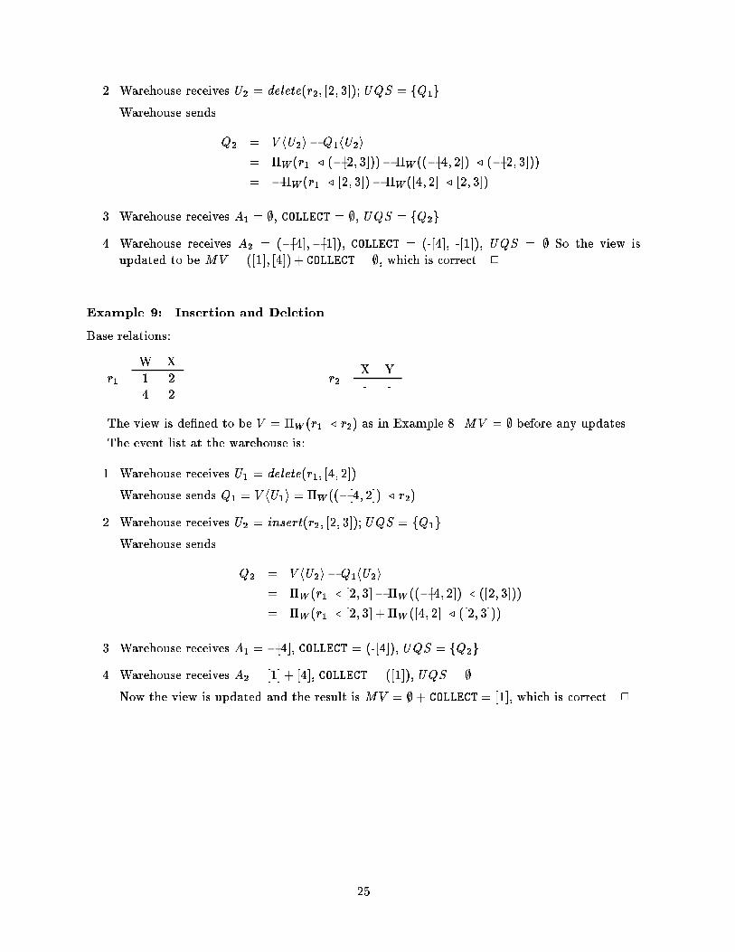
Example 9: Insertion and Deletion

Base relations:

r1

W X

1 24 2

r2X Y

- -

The view is de�ned to be V = �W (r1 ./ r2) as in Example 8. MV = ; before any updates.

The event list at the warehouse is:

1. Warehouse receives U1 = delete(r1; [4; 2])

Warehouse sends Q1 = V hU1i = �W ((�[4; 2]) ./ r2)

2. Warehouse receives U2 = insert(r2; [2; 3]); UQS = fQ1g.

Warehouse sends

Q2 = V hU2i � Q1hU2i

= �W (r1 ./ [2; 3]��W ((�[4; 2]) ./ ([2; 3]))

= �W (r1 ./ [2; 3] + �W ([4; 2] ./ ([2; 3]))

3. Warehouse receives A1 = �[4], COLLECT = (-[4]), UQS = fQ2g.

4. Warehouse receives A2 = [1] + [4], COLLECT = ([1]), UQS = ;.

Now the view is updated and the result is MV = ;+ COLLECT = [1], which is correct. 2

25

B Correctness of the Eager Compensating Algorithm

In this section we provide a correctness proof for the Eager Compensating Algorithm (ECA) aspresented in Section 5. Theorem B.1 shows that ECA is strongly consistent by proving that it isboth consistent and convergent. Before getting to the theorem, we need to establish �ve lemmas.

First, we claim that not all events will a�ect outcome of a query evaluation. For example, if asource event se has type S qu, then the base relations are not modi�ed. Consequently, the resultof evaluating another query before or after se are the same.

Formally, let sei be an arbitrary source event; the source state before sei is ssi�1 and after isssi. Let wei be a warehouse event and the warehouse state before wei is wsi�1 and after is wsi.

Lemma B.1 Independent events using ECA.

sei has type S qui =) V [ssi�1] = V [ssi], Q[ssi�1] = Q[ssi]

wei has type W upi =) V [wsi�1] = V [wsi]

wei has type W ansi with UQS 6= ; =) V [wsi�1] = V [wsi]

Proof: Obvious from the de�nition of events (Section 3) and events described in ECA. 2

With ECA, the triggering relationship among source and warehouse events is as shown inFigure B.6.

(ss )j

(ws )j

S_upj

W_upj W_ans j

S_qu j

UjQj

Aj

(ss )j-1

(ws )j-1

SOURCE

WAREHOUSE

Figure B.6: Triggering relations among events.

Since there is a one-to-one correspondence between updates and the four events they trigger,in the rest of the appendix we will label events by the id of the update that generated them.Speci�cally, let U1; U2; : : : be the updates that occurred during the execution of ECA algorithm.For each Uj , the events it triggers are S upj ,W upj , S quj and W ansj . Also, let Qj be the queryinvolved in the processing of Uj and Aj be the answer relation of Qj . According to Lemma B.1,at the source only events of type S up a�ect query evaluation, so we can assume the source stateonly change after each S up event, that is, we can label the source state before S upj as ssj�1and label it after S upj as ssj . Similarly, assume warehouse states only change after each typeW ans events.

In the next lemma, we show how a type S up event a�ects the evaluation of a query. AssumeQ is an arbitrary query and is targeted for execution before a source update Uj(at state ssj�1).However it is actually executed after Uj(at state ssj).

Lemma B.2 Q[ssj�1] = Q[ssj ]�QhUji[ssj ] for any query Q.

Proof:

Consider a term T in Q as de�ned by Formula 4.1: T = �X(�C(~r1 � ~r2 � : : :� ~rn)). AssumeUj is an update on relation rm. If rm is not used in T , then T hUji = ;, and T [ssj ] = T [ssj�1].

26

Therefore we have T [ssj ] = T [ssj�1] + T hUji[ssj ] holds. If rm is used in de�ning T , then for rlother than rm, ~rl[ssj ] = ~rl[ssj�1]. And ~rm[ssj ] = ~rm[ssj�1] + tuple(Uj). Then

T [ssj ] = �X(�C(~r1[ssj ]� ~r2[ssj ]� : : :� ~rm[ssj ]:::� ~rn[ssj ]))

= �X(�C(~r1[ssj ]� ~r2[ssj ]� : : :� (~rm[ssj�1] + tuple(Uj)) : : :� ~rn[ssj ]))

= �X(�C(~r1[ssj�1]� ~r2[ssj�1]� : : :� ~rm[ssj�1] : : :� ~rn[ssj�1])) +

�X(�C(~r1[ssj ]� ~r2[ssj ]� : : :� tuple(Uj) : : :� ~rn[ssj ]))

= T [ssj�1] + T hUji[ssj ]:

Since Q =P

i Ti de�ned by Formula 4.2 is a sum of terms, we have Q[ssj ] = Q[ssj�1] +QhUji[ssj ]. Thus Q[ssj�1] = Q[ssj ]�QhUji[ssj ]. 2

In ECA, if UQS(W ansj) = ;, then the warehouse updates the materialized view MV. Thefollowing lemma states that when the warehouse updates MV, the last answer it gets(Aj) is theintended one for Qj .

Lemma B.3 UQS(W ansj) = ; =) Aj = Qj [ssj ].

Proof:

Assume there exists an S upm, such that S upj < S upm < S quj . Then from the triggeringrule described in Section 3 we know that W upj < W upm < W ansj , and W ansj < W ansm.Therefore, Qm 2 UQS(W ansj) and this implies that UQS(W ansj) 6= ;. This is a contradiction,therefore all source events between S upj and S quj(if there are any) must be of type S qu. ByLemma B.1 and our labeling convention, the source state right before S quj is still ssj , and Aj isevaluated at this state, Aj = Qj [ssj ]. 2

De�nition: An event of type W ans updates the materialized view at the warehouse whenits UQS is empty. De�ne W ansi be the Previous-Updating-Event of a warehouse event we ifW ansi < we, UQS(W ansi) = ;, and 6 9W ansm such that W ansi < W ansm < we andUQS(W ansm) = ;.

The next lemma shows that for two consecutive updates on the warehouse view, if the �rstone updates the view into a consistent state, then so does the second one.

Lemma B.4 Assume UQS(W ansj) = ; andW ansi is the Previous-Updating-Event ofW ansj .

Then V [wsi] = V [ssi] =) V [wsj ] = V [ssj ].

Proof: We know that the updates occurring between Ui and Uj (if any) are Ui+1, Ui+2, : : :,

Uj�1. Before updating MV at event W ansj , the COLLECT set is COLLECT =Pj

l=i+1Al

since the last time COLLECT was set to empty was at event W ansi. Furthermore we haveV [wsj ] = V [wsi] + COLLECT .

Now we can reduce the proof that V [wsj ] = V [ssj ] assuming V [wsi] = V [ssi] to the proof of

the following equation with COLLECT =Pj

l=i+1Al:

V [ssi] + COLLECT = V [ssj ] (B.3)

The proof of Equation B.3 is done by induction on the number of updates between Ui and Uj ,which is m = j � i� 1 � 0.

27

1. Base case: m = 0.

There is no update between Ui and Uj so Ui and Uj are consecutive updates. SinceUQS(W ansj) = ;, we have Qj = V hUji � ; = V hUji.

V [ssi] +Aj = V [ssi] +Qj [ssj ]

= V [ssi] + V hUji[ssj ]

= V [ssj ]

(Lemma B:3)

(ECA)

(Lemma B:2)

Thus, Equation B.3 holds for the base case.

2. Induction step:

Induction hypothesis: Assume Equation B.3 holds for all m < c.

When m = c, we have c updates between Ui and Uj . Let us refer this scenario with c

updates as Scenario S. In Scenario S, some of the queries in Qi+1 : : :Qj�1 are evaluatedbefore Uj occurs at the source, some after.

Let

Qbefore =j�1Xl=i+1

Ql =2UQS(W upj )

Ql and Qafter =j�1Xl=i+1

Ql2UQS(W upj)

Ql

Correspondingly, let

Abefore =j�1Xl=i+1

Ql =2UQS(W upj )

Al and Aafter =j�1Xl=i+1

Ql2UQS(W upj )

Al

SoCOLLECT = Abefore + Aafter + Aj (B.4)

Let Scenario S0 be exactly the same as Scenario S except Uj and all four correspondingevents do not occur. In Scenario S 0 we label all events and states with a prime. Thus theupdates are U 0

1; U0

2; : : :, the queries are Q0

1; Q0

2; : : :, and so on. Many of the S0 events andstates correspond to the ones in S. In particular, V 0 = V (we have the same view), and8l; i � l � j � 1, U 0

l = Ul, Q0

l = Ql and ss0

l = ssl.

Since Uj is absent in Scenario S0, UQS(W ans0j�1) = ;. There are c � 1 < c updatesbetween Ui and Uj�1. By induction hypothesis we have

V 0[ss0i] + COLLECT 0 = V 0[ss0j�1] (B.5)

In Scenario S 0, COLLECT 0 is the sum of answers A0

i though A0

j�1. Let us divide the answersinto two sets:

A0

before = answers to the queries that constitute Qbefore

A0

after = answers to the queries that constitute Qafter

Thus, COLLECT 0 = A0

before +A0

after, Equation B.5 can be written as

V [ssi] + A0

before +A0

after = V [ssj�1] (B.6)

28

Abefore are those answers computed before Uj in Scenario S, they are computed at the samestate in Scenario S0, thus Abefore = A0

before.

Aafter contains those answers that were computed after Uj occur in Scenario S. SinceUQS(W ansj) = ;, by similar arguments to those in Lemma B.3, we know that all answersin Aafter are computed at state ssj = state(S upj):

Aafter = Qafter[ssj ] (B.7)

In Scenario S0, answers in A0

after must be computed after Uj�1 occurs, otherwise they willnot be evaluated after Uj in Scenario S. So A0

after = Qafter[ssj�1], and Equation B.6becomes:

V [ssi] +Abefore +Qafter[ssj�1] = V [ssj�1] (B.8)

Furthermore, we know that Qj = V hUji � QafterhUji from Algorithm ECA. This gives usQj [ssj ] = V hUji[ssj ] � QafterhUji[ssj ]. From Lemma B.2 we have that Qafter[ssj�1] =Qafter[ssj ]� QafterhUji[ssj ]. Subtracting the latter from the former equation we obtain

Qafter[ssj ] +Qj [ssj ] = Qafter[ssj�1] + V hUji[ssj ] (B.9)

The intuitive meaning of Equation B.9 is that if the queries in Qafter and Qj are evaluatedin state ssj as in Scenario S, the result will be the same as evaluating those queries in Qafter

in state ssj�1 as in Scenario S0, and adding the term V hUji[ssj ] that re ects the e�ect ofUj on the view.

Combining all of our results we can show that

V [ssi] + COLLECT

= V [ssi] + Abefore + Aafter + Aj

= V [ssi] + Abefore + Qafter[ssj ] + Aj

= V [ssi] + Abefore + Qafter[ssj ] + Qj [ssj ]

= V [ssi] + Abefore + Qafter[ssj�1] + V hUji[ssj ]

= V [ssj�1] + V hUji[ssj ]

= V [ssj ]

( B:4)

( B:7)

(Lemma B:3)

( B:9)

( B:8)

(Lemma B:2)

This shows that Equation B.3 holds in Scenario S, and completes the induction proof. As statedearlier, Equation B.3 is su�cient to prove Lemma B.4. 2

Lemma B.5 Assume V [ws0] = V [ss0], then UQS(W ansj) = ; =) V [wsj] = V [ssj ] for any j.

Proof: The proof is done by induction on j.

1. Base case: j = 1.

Assume there is an 'empty update' U0 which occurs before any updates and its four events(which are also empty) are processed before any other events. After S up0 the source state

29

is ss0 and after W ans0 the warehouse state is ws0. Since there's no pending queries whenW ans0 is processed, W ans0 is the Previous-Updating-Event of W ans1.

Since V [ws0] = V [ss0] and UQS(W ans1) = ;, by Lemma B.4 we have V [ws1] = V [ss1].

2. Induction step: Induction hypothesis: the lemma holds for any j < c (c > 1).

When j = c, let W ansi be the Previous-Updating-Event of W ansj . So i < c and byinduction hypothesis we have V [wsi] = V [ssi]. Then from Lemma B.4 we can proveV [wsj ] = V [ssj ].

2

Theorem B.1 Algorithm ECA is strongly consistent for a �nite sequence of updates U1; U2; : : : ; Uk.

Proof:

Assume V [ws0] = V [ss0], the warehouse is in a consistent state with the source before anyevents occur.

Consistent:

The de�nition of consistency is given in Section 3. For every pair of warehouse states wsi <wsj with corresponding events wei � wej , let W ansi0 be the Previous-Updating-Event of weiand W ansj0 be the Previous-Updating-Event of wej . W ansi0 � W ansj0 obviously. FromLemma B.1, we know V [wsi] = V [wsi0 ] and V [wsj ] = V [wsj0 ].

Since the UQS of both W ansi0 and W ansj0 are empty, Lemma B.5 gives that V [wsi0 ] =V [ssi0 ] and V [wsj0 ] = V [ssj0 ]. Also, W ansi0 � W ansj0 implies ssi0 � ssj0 .

So there exist ssn = ssi0 � ssl = ssj0 such that V [wsi] = V [ssn] and V [wsj ] = V [ssl]. Byde�nition, ECA is consistent.

Convergent:

UQS(W ansk) = ; since Uk is the last update. Lemma B.5 gives V [wsk] = V [ssk ]. At thesource, the last update is in S upk and after that, all events(if any) have type S qu. So ssk isthe �nal source state. At the warehouse, W ansk is the last event so wsk is the �nal warehousestate. Thus ECA is convergent.

Since ECA is consistent and convergent, it is strongly consistent. 2

30

C Sketch of Proof of Correctness for ECA-Key algorithm

Consider a warehouse event wef where UQS(wef) = ;. The warehouse state right after thisevent, state(wef ) = wsf . Let F be the set of all updates that have been seen at the warehouseby wef . Let Uf 2 F be the last update received before or by wef .

Let sef be the S up source event that processed Uf , and let ssf be the source state immediatelyafter sef . In the rest of this sketch we discuss how to show that V [ssf ] = V [wsf ]. Given this,it is straightforward to see that ECAK is strongly consistent, since the materialized view onlychanges at the warehouse when UQS = ;.

We can show that V [ssf ] = V [wsf ] by contradiction and considering the various cases. Thatis, assume that V [ssf ] 6= V [wsf ]. Then there must be a tuple t that is either missing from V [wsf ]or is an extra tuple in V [wsf ]. (In what follows, we do not have to worry about t appearing morethan once either at the source or the warehouse due to our key condition.)

Case I: t 2 V [ssf ] and t 62 V [wsf ].

Subcase I(a): There is (at least one) insert at the source (before sef ) that generates t. Let Ui bethe last of these events. Insert Ui adds a tuple at the source that contains one of the keys involvedin t. (Recall that t has a key value for each of the relations involved in the view de�nition.)

Note there can be no deletes involving a t key after Ui is processed at the source (at least notbefore or at sef ). If there were, they would remove t from V [sef ], a contradiction.

Under ECAK , Ui gets propagated to the warehouse, a query Q is generated, answered at thesource, and an answer returned to the warehouse. At the warehouse, both the processing of Uiand the receipt of the Q answer must occur before or at wef . (If Ui were received after wef ,then Ui 62 F and Ui must have been processed after sef . If the Q answer arrived after wef , thenUQS(wef) would not have been empty.) When Q is processed at the source, it sees all the keyvalues involved in t, so the answer to Q contains t. Thus, t is inserted into the materialized view.Because there are no deletes a�ecting t at the source between the processing of Ui and sef , therecan be no such deletes at the warehouse, and t remains until wef , a contradiction.

Subcase I(b): There are no inserts at the source that generate t. This means that t must havebeen in V [ss0], where ss0 is the initial source state. Since the initial materialized view is correct,t must also be in V [ws0].

We can now proceed similarly to Case I(a), arguing that there are no deletes a�ecting t at thesource (before sef ) and hence no such deletes at the warehouse. Thus, t remains at the warehouse,a contradiction.

Case II: t 62 V [ssf ] and t 2 V [wsf ].

Subcase II(a): There is at least one delete at the source that involves a t key value. The proofis analogous to Case I(a), with one extra case to consider. We consider the last such sourcedelete Ud, where sed is the processing of Ud at the source and wed is the processing of Ud at thewarehouse. Clearly, wed deletes t from the materialized view. Since t 2 V [wsf ], it must have beenreinserted. Notice that there are no inserts that could generate t at the source after sed, so therecannot be any corresponding inserts that warehouse. However, it could be the case that an insertUj occurring at the source before Ud, could generate an answer that is processed at the warehouseafter wed, adding t. The query generated for Uj must have been processed at the source after sed(else the answer would have arrived before wed). Since the query is executed at the source afterUd is processed, it does not see one of the key values of t (i.e., the one deleted by Ud). Thus, thereis no way the answer could contain t, and t is not added to the materialized view, a contradiction.

31

Subcase II(b): There are no source deletes that involve a key value of t. Therefore t mustnot be in the initial V [ss0], and since the initial materialized view is correct, t is not in V [ws0].Since somehow t appears in V [wsf ], it must have been inserted by some answer received at thewarehouse. Say sek is the source event that generates the answer. At that point V [state(sek)]must contain t. Since there are no deletes a�ecting t at the source, then t remains, a contradiction.

D Performance Evaluation

D.1 Recomputing the View

The following is a description of the \recompute view" strategy (RV), it updates MV after everys source updates.

Algorithm D.1 (Algorithm RV)

Events at the source are as in Algorithm 5.1. At the warehouse (initially Count = 0):

� W upi: receive Ui;let Count = Count+1;if Count = sthen flet Count = 0; let Qi = V ;

send Qi to the source;trigger event S qui at the sourceg

� W ansi: receive Ai;let MV Ai

(end algorithm)

D.2 Performance Based on Number of Bytes Transferred

1. RV best and worst case computation:

Let card(ri) be the cardinality of relation ri. The total bytes transferred is equal to the sizeof the resulting view:

BRVBest = (W;Zbytes)� ( number of tuples in the resulting view relation)

= S � � � (card(r1)� J(r2; X)� J(r3; Y ))

= S�CJ2

For the worst case, the view is recomputed after each update, i.e., three times:

BRVWorst = 3�BRVBest = 3S�CJ2

2. ECA best case computation:

The warehouse events occur in this order: U1; Q1; A1; U2; Q2; A2; U3; Q3; A3

Using ECA, we know

32

Q1 = V hU1i = �W;Z(�cond(t1 ./X r2 ./Y r3))

Q2 = V hU2i = �W;Z(�cond(r1 ./X t2 ./Y r3))

Q3 = V hU3i = �W;Z(�cond(r1 ./X r2 ./Y t3))

The size of A1 can be evaluated as: B = S � � � 1� J(r2; X)� J(r3; Y ) = S � � � J2

The size of A2 and A3 can be estimated in a similar fashion.

BECABest = 3S�J2

3. ECA worst case computation:

The event order is: U1; Q4; U2; Q5; U3; Q6; A4; A5; A6

The queries are:

Q4 = V hU1i = Q1

Q5 = V hU2i �Q4hU2i = V hU2i � �W;Z(�cond(t1 ./X t2 ./Y r3))

Q6 = V hU3i�Q4hU3i�Q5hU3i = V hU3i��W;Z(�cond(t1 ./X r2 ./Y t3))��W;Z(�cond(r1 ./Xt2 ./Y t3)) + �W;Z(�cond(t1 ./X t2 ./Y t3))

Notice that the cost for the �rst terms of Q4, Q5, Q6 is equal to BECABest. For the secondterm in Q5, �W;Z(�cond(t1 ./X t2 ./Y r3)), B = S � � � J(r3; Y ), i.e., B = S�J . The costof the second and third terms in Q6 is the same. The cost of the last term in Q6 is 0; itdoes not have to be sent to the source for evaluation.

For the total cost, the costs for these terms are added. (Recall that \�" is not a setdi�erence operator; it is a union of signed tuples.) Thus BECAWorst = BECABest + 3S�J ,or BECAWorst = 3S�J(J + 1).

4. For the k update case, we assume that the �rst three updates are as before, and then weget k � 3 additional ones.

For RV it is easy to see thatBRVBest does not change, andBRVWorst = kBRVBest = kS�CJ2.

For the best ECA case, it is easy to see that our computation above generalizes toBECABest =kS�J2.

For the ECA worst case, consider a fourth update U4 on relation r1. Assuming all queries areexecuted after all updates (worst case), ECA issues queries Q4, Q5, Q6 as before. The lastquery is Q7 = V hU4iQ1hU4iQ2hU4iQ3hU4i. That is, Q7 = V hU4i� V hU1; U4i� V hU2; U4i+V hU1; U2; U4i� V hU3; U4i+V hU1; U3; U4i+ V hU2; U3; U4i�V hU1; U2; U3; U4i. Since U1 andU4 update the same relation, all terms of the form V hU1; U4; :::i are empty. Similarly, allterms with three or more updates are empty (no compensating query needs to be sent sinceall data needed is already at the warehouse). This leaves the �rst term with data transfercost S�J2 and two compensating queries with costs S�J . Notice that the cost would bethe same if U4 had modi�ed any of the two other relations.

So, in general, we see that the cost of processing update Uj is S�J2 (for the Qj term V hUji)

plus a term S�J (for V hUj ; Upi) for each previous update Up such that rel(Uj) 6= rel(Up).If we assume that updates access any of the three relations with equal probability, then thecost for Uj is S�J

2 + (2(j � 1)=3)S�J . Adding the terms from 1 to k we get BECAWorst =kS�J2 + k(k � 1)S�J=3.

33

D.3 Performance Based on I/O

D.3.1 Scenario 1

1. RV best and worst case computation:

Assuming that J is not too small, the best strategy is for the source to read into memoryall three relations.

IORVBest = dcard(r1)

Ke+ d

card(r2)

Ke+ d

card(r3)

Ke = 3d

C

Ke = 3I

where I = dCKe is the number of IOs needed to read an entire base relation.

In the worst case, RV computes the view three times, so IORVWorst = 3� IORVBest = 9I .

2. For the ECA best case, we have the same three queries Q1, Q2, Q3 as in Section D.2. Letus �rst assume that J < I so it is best to use the indexes for evaluating all the queries.

For Q1, we use the X value in t1 to fetch the matching r2 tuples (using the X index on r2).Since the X index is clustered, all the r1 tuples are contiguous. This gives the �rst termbelow. Then, for each of the J(r2; X) tuples found, we get the matching r3 tuples, givingus the second term. Thus,

IO1 = dJ(r2; X)

Ke + (J(r2; X)� d

J(r3; Y )

Ke):

Assuming that J � K (which holds for the value ranges we are interested in here), thisreduces to

IO1 = 1 + J:

As discussed in the main body of the paper, the select condition in Q1 is evaluated afterthe join since it involves W and Z attributes. This implies that the condition does not saveus any I/Os. Note that we did not consider caching e�ects: whenever we probe a relation,we go to disk to read the block. Hence, the results for ECA are pessimistic, even for theevaluation of a single term.

For Q2, we use the t2 tuple values to probe the r1 and r3 indexes. Thus,

IO2 = dJ(r1; X)

Ke + d

J(r3; Y )

Ke = 2:

For Q3, we have to use an un-clustered index to probe r2, so for each of the J(r2; Y ) tupleswe need an I/O. This gives us the �rst term below. Then we use the X index to probe r1giving us the second term.

IO3 = J(r2; Y ) + (J(r2; Y )� dJ(r1; X)

K)e = J + J:

Therefore IOECABest = IO1 + IO2 + IO3 = 3J + 3:

If J � I , Q3 can be best evaluated by reading in both r1 and r2, for a total cost of 2I . ForQ1, it is also better to read in r3 fully (cost is I) rather than piecemeal (cost J), so the costof Q1 is 1+ I . Query Q2 is still done best with indexes. Thus, the total cost when J � I is3I + 3.

34

In general, and assuming that the query optimizer can select the best plan, the cost ofevaluating the three queries will be IOECABest = 3min(J; I) + 3.

3. ECA worst case computation:

For V hU1i; V hU2i and V hU3i, the number of I/Os is the same as obtained for the best case.

For term the �W;Z(�cond(t1 ./X t2 ./Y r3)) in Q5, IO = dJ(r3; Y )=Ke = 1

Similarly, for the extra terms in Q6 we have IO = dJ(r2; X)=Ke+ dJ(r1; X)=Ke = 2

Thus, IOECAWorst = IOECABest+ 3 = 3min(J; I) + 6

D.3.2 Scenario 2

We assume there are no indices on any attributes. We also assume that the memory can onlyhold three blocks, which are used for a nested join algorithm.

1. RV computation:

To compute r1 ./ r2 ./ r3, the source can load one r1 and one r2 block into memory andloop through r3. Then it repeats this for all possible pairs of r1, r2 blocks. Thus,

IORVBest = I3

IORVWorst = 3� IORVBest = 3I3.

2. IOECABest computation:

Using Q1 as an example, the source can load two blocks of r2 into memory and loop throughthe r3 records (number of I/Os is I). This is repeated dC=(2K)e times, so IO1 = I � I 0,where I 0 = dC=(2K)e is the number of double-block bu�ers needed to hold a relation.

The cost for the other queries is the same, so altogether, IOECABest = 3II 0.

3. IOECAWorst computation:

For each of the three extra terms in the compensating queries we need to read a relation,so IOECAWorst = 3II 0+ 3I = 3I(I 0+ 1)

D.3.3 k Update Case

We extend the Scenario 1 and 2 results for the case of k updates. The analysis is similar to thatat the end of Section D.2. For simplicity, assume that J < I .

For Scenario 1:

1. IORVBest = 3I since the view is still recomputed once.

2. IORVWorst = 3kI .

3. IOECABest = k� (3J +3)=3 = k(J +1) because we assumed updates have equal probabilityon any of the three relations, and the total IO for three updates on three relations are 3J+3as we computed before (and J < I).

4. IOECAWorst = k(J + 1) + k(k � 1)=3

The cost of evaluating V hUji is J +1, and the cost of evaluating V hUj ; Upi is 1, so the totalisP

j=1 k((J + 1) + 2(j � 1)=3) = k(J + 1) + k(k � 1)=3.

35

For Scenario 2:

1. IORVBest = I3 since the view is still recomputed once.

2. IORVWorst = kI3.

3. IOECABest = kII 0

4. IOECAWorst = kII 0 + Ik(k � 1)=3:

To compute the last expression, we note that for update Uj , the query Qj contains V hUjiplus (on average) 2(j� 1)=3 terms of the form V hUj ; Upi where rel(Uj) 6= rel(Up). The costof evaluating Qj is thus II

0+ 2(j � 1)I=3. Adding from Q1 to Qk we obtain the expressionabove.

36