vii. autonomous flight control and software · pdf filevii. autonomous flight control and...
TRANSCRIPT
VII. Autonomous Flight Control and Software
72 J.-B. Brachet, R. Cleaz, A. Denis, A. Diedrich, D. King, P. Mitchell, D. Morales,
J. Onnée, T. Robinson, O. Toupet, B. Wong

A. Guidance Approaches
c) Traditional or Model Based Methods
1. Leader-Follower Station-Keeping
Leader-follower station-keeping is a relatively standard guidance method that has been well explored in the literature, starting with Hummel [10] and constantly improved upon and validated in various simulations [6,11,13,14,16,17]. In this method the control algorithm tries to maintain a static position relative to another aircraft in the formation. This static position is pre-determined, either by aerodynamic theory that is known to be incomplete, or experimental data that is expensive to obtain (and impractical to do for every possible formation flight configuration).
There are two types of station keeping, “leader mode”, where each aircraft maintains a relative position to a designated leader aircraft [6], and the more commonly investigated “front” mode where relative position is held in the vortex of the wingman directly ahead of the trailing aircraft [5,6,8,10,11,13,14,16,17]. The wingman directly ahead of a trailing aircraft may coincide with the formation leader, but this isn’t necessarily so as formation numbers rise above two.
Through NASA’s Autonomous Formation Flight (AFF) program, this method was able to maintain a relative position within 9ft of desired 100% of the time between two F/A-18s in a flight test [8]. This makes the leader-follower method the only station-keeping algorithm to date to be implemented in formation flight. However, these results were not obtained with the trailing aircraft in the wingtip vortex.
2. Trajectory Tracking
Trajectory tracking is another method which has found frequent use in many control problems, particularly for unmanned aerial vehicles (UAVs) [7,11]. The algorithm attempts to have the vehicle follow a pre-defined set path through space (most likely the great circle trajectory) as closely as possible. In the formation flight case, these trajectories are offset by the exact amount that is required for the trailing aircraft to be in the wingtip vortices of their wingmen ahead.
This method of guidance, in its pure form, is appropriate if the mission has a set trajectory with no arbitrary maneuvers that weren’t planned beforehand. It is the easiest method to implement from a technical standpoint, and may not require relative position measurements depending on the implementation.
3. Formation Geometry Center
This concept is based off of observation of the natural flight behavior of birds that maintain a defined geometrical shape, but if one or more of the birds loses its position in the formation, the flock waits (or holds back) for those birds to rejoin the formation. The original trajectory is modified to accomplish this. So this algorithm tries to maintain formation geometry (thus, relative positions can be maintained) while at the same time tracking a prescribed path for each aircraft. If an aircraft loses its position, the formation senses it, acts together to restore geometry, then moves back to tracking the correct path. This combines pure trajectory tracking with a variant of the station-keeping concept. The formation
73 J.-B. Brachet, R. Cleaz, A. Denis, A. Diedrich, D. King, P. Mitchell, D. Morales,
J. Onnée, T. Robinson, O. Toupet, B. Wong
geometry center (FGC) itself is an imaginary point that depends on the integral of the average of formation speeds, headings and flight path angles. Simulations of this method were performed in [7] on a two aircraft V-formation that showed good results.
d) Non-Model Based Methods
1. Neural Networks
Neural Networks (hereafter referred to as NN) are software programs that have the ability to be trained by presenting the program examples of input and the corresponding desired output. NN are receiving a lot of attention in many different areas, primarily NOT in formation flight, but it has been tried in very limited simulation. Reference [15] presents a framework for getting a NN to tell output relative position based upon wake effects the trail aircraft is senses and shows that it is possible in practice. Extreme care must be taken to have an excellent training set for good results, because if the training set is different than actual conditions the algorithm will not act in a predictable way. Neural networks have also been mentioned in [5] by Boeing as an area for possible further development in the NASA AFF project.
2. Performance/Extremum Seeking
The objective of this algorithm is to minimize a performance parameter, in formation flight typically the trailing aircraft’s trim pitch angle or thrust. It does not need to know any information about a vortex model. This area is still quite under-developed and most theory [2,4] places the aircraft near the desired position, then moves opposite the gradient of the measured performance function. This requires the introduction of a dither (periodic) signal for the system to sense the gradient, which is highly undesirable. Other methods using neural networks to “sense” the gradient have also been tried [12]. Simulations have been done with 2 F/A-18s [12] and C5s [2] in formation, but there have not yet been any flight tests.
e) Other
1. Vortex Shaping
Vortex shaping is an idea that has not yet been explored in formation flight literature, but has been discussed informally at MIT, Stanford and Boeing. There may also be some non-formation flight applications. What this involves is a manipulation of the wingtips/wings of the aircraft creating the vortices so that the vortices themselves move instead of the trailing aircraft. In other words, the vortex is brought to an optimal location based on where the trailing aircraft is instead of the other way around. Major limitations of this method are that it would require non-trivial structural changes to the wings on existing aircraft, and the fact that a good enough model of the wake of an aircraft does not exist to be able to predict with enough accuracy where aircraft geometry changes will move the vortices.
2. H-Infinity Methods
This is a relatively new control method that takes performance and stability goals for the system and translates them into limits on the infinity norm of the transfer function for the MIMO system. The frequency response of the system is manipulated to achieve desired
74 J.-B. Brachet, R. Cleaz, A. Denis, A. Diedrich, D. King, P. Mitchell, D. Morales,
J. Onnée, T. Robinson, O. Toupet, B. Wong
results. The basic philosophy is to minimize the worst case control scenario. This type of control was mentioned as a possible future direction in [5] for the NASA AFF project.
B. Control-Configured Vehicles
Control-configured vehicles may be utilized for formation flight as a way to possibly complete in-flight adjustments more efficiently. This would involve utilizing direct lift and side force actuators to accomplish lateral and vertical motions to correct small errors in position. Doing so would mean that trailing vortices would not move up or down due to pitch or roll. Using this method, auxiliary engines could be used that are designed for finer adjustments that would use less fuel overall. Whether this is worth pursuing will depend on the possible formation fuel savings, which are unknown. Control-configured vehicles have been utilized in other applications such as UAVs and even for production fighter jets (ex. Dassault/Dornier Alpha Jet Direct Side Force Control (DSFC) demonstrator aircraft of the German Air Force) but not for formation flight.
C. String Stability
String stability is a measure of how errors propagate through a series of interconnected systems. In the case of formation flight, string stability is determined by whether position errors in the front of the formation get larger or smaller as they move down the chain. This is a topic that has been well explored for platoons of automobiles or similar types of land vehicles, but not very much in the specific formation flight domain. It is known that string stability of land vehicles can be achieved with constant separation distance if each vehicle knows the relative velocity or position of the lead vehicle and the one in front of it (they may be the same) [19,20]. If separation distance can vary with speed, then only the absolute velocity of the vehicle and the relative velocity of the vehicle in front are required. It has been hypothesized in [18] that these same requirements will result in string stability of formation flight as well, though there are complicating factors.
In [1], the string stability of a formation flight of 7 F/A-18 aircraft in an echelon formation was examined using both linear and non-linear models. They used a leader-follower approach as described above and found that indeed the formation was string unstable in this configuration. However, the results indicated that string instability may not degrade performance enough to worry about it, especially for smaller formations. Another limiting factor that was discovered in this analysis was the level of acceleration that the pilots would experience. A measure of this is the “ride quality” given by the motion sickness dose values (MSDV) issued by the ISO. In essence, MSDV is a frequency-weighted acceleration in the z-direction. With more aggressive control gains, the MSDV can get above a level where 10 percent of the general population would vomit after an hour of flight.
D. Autopilot & Software Capabilities
Autopilots can do just almost everything in formation flight. For form up, a pilot could activate a formation flying autopilot which would track to a specific point relative to another aircraft, provided to begin with the two planes were close enough. To leave a formation, pilots could specify a new relative position outside the formation before taking the controls. Rough algorithms in simulation also have been able to perform more dynamical tasks such as switching
75 J.-B. Brachet, R. Cleaz, A. Denis, A. Diedrich, D. King, P. Mitchell, D. Morales,
J. Onnée, T. Robinson, O. Toupet, B. Wong

leaders in a formation (as described in [10] for “equal power” formation) and changing formation geometry when the number of aircraft in the formation changes due to one leaving or joining up.
Software is not up to flight critical standards for formation flight just yet. As such (and even when it is), mid-air collision is always a concern. Warnings can be provided to the pilot and the formation flight autopilot can disengage automatically when minimum separation distances or maximum separation rates passed. The normal airplane autopilot can still be engaged at this point if desired. Indeed, this was exactly the case for the NASA AFF project. In order to prevent system failures, redundancy needs to be build into the software.
76 J.-B. Brachet, R. Cleaz, A. Denis, A. Diedrich, D. King, P. Mitchell, D. Morales,
J. Onnée, T. Robinson, O. Toupet, B. Wong
References
[1] Allen, M.J., Ryan, J., Hanson, C.E., and Parle, J.F., “String Stability of a Linear Formation Flight Control System,” AIAA Paper 2002-4756, Aug. 2002.
[2] Binetti, P., Ariyur, K.B., Krsti , M., and Bernelli, F., “Formation Flight Optimization Using Extremum Seeking Feedback,” AIAA Journal of Guidance, Control and Dynamics, Vol. 26, No. 1, 2003, pp.132-142.
[3] Blake, W.B., and Multhopp, D., “Design, Performance and Modeling Considerations for Close Formation Flight,” AIAA Paper 98-4343, Aug. 1998.
[4] Chichka, D.F., Speyer, J.L., and Park, C.G., “Peek Seeking Control with Application to Formation Flight,” Proceedings of the 38th IEEE Conference on Decision and Control, pp. 2463-2470, Phoenix, AZ, Dec. 1999.
[5] Cobleigh, B., “Capabilities and Future Applications of the NASA Autonomous Formation Flight (AFF) Aircraft,” AIAA Paper 2002-3443, May 2002.
[6] Guilietti, F., Pollini, L., and Innocenti, M., “Autonomous Formation Flight,” IEEE Controls System Magazine, Vol. 20, No. 6, 2000, pp. 34-44.
[7] Guilietti, F., Pollini, L., and Innocenti, M., “Formation Flight Control: A Behavioral Approach,” AIAA Paper 2001-4239, Aug. 2001.
[8] Hanson, C.E., Ryan, J., Allen, M.J., and Jacobson, S.R., “An Overview of Flight Test Results for a Formation Flight Autopilot,” AIAA Paper 2002-4755, Aug. 2002.
[9] Houck, S., and Powell, J.D., “Visual, Cruise Formation Flying Dynamics,” AIAA Paper 2000-4316, Aug. 2000.
[10] Hummel, D., “The Use of Aircraft Wakes to Achieve Power Reduction in Formation Flight,” Proceedings of the Fluid Dynamics Panel Symposium, AGARD, 1996, pp. 1777-1794.
[11] Larson, G., “Autonomous Formation Flight,” Presentation to MIT 16.886 Class, 05 Feb. 2004.
[12] Lavretsky, E., Hovakimyan, N., Calise, A., and Stepanyan, V., “Adaptive Vortex Seeking Formation Flight Neurocontrol,” AIAA Paper 2003-5726, Aug. 2003.
[13] Lavretsky, E., “F/A-18 Autonomous Formation Flight Control System Design,” AIAA Paper 2002-4757, Aug. 2002.
[14] Misovec, K. “Applied Adaptive Techniques for F/A-18 Formation Flight,” AIAA Paper 2002-4550, Aug. 2002.
[15] Pollini, L., Guilietti, F., and Innocenti, M., “Sensorless Formation Flight,” AIAA Paper 2001-4356, Aug. 2001.
[16] Proud, A.W., Pachter, M., and D’Azzo, J.J., “Close Formation Flight Control,” Proceedings of the AIAA Guidance, Navigation and Control Conference, pp. 1231-1246, Portland, OR, Aug. 1999.
[17] Schumacher, C.J., and Singh, S.N., “Nonlinear Control of Multiple UAVs in Close-Coupled Formation Flight,” AIAA Paper 2000-4373, Aug. 2000.
77 J.-B. Brachet, R. Cleaz, A. Denis, A. Diedrich, D. King, P. Mitchell, D. Morales,
J. Onnée, T. Robinson, O. Toupet, B. Wong

[18] Wolfe, J.D., Chichka, D.F., and Speyer, J.L., “Decentralized Controllers for Unmanned Aerial Vehicle Formation Flight,” AIAA Paper 96-3833, Jul. 1996.
[19] Kaminer, I., Pascoal, A., Hallberg, E., and Silvestre, C., “Trajectory Tracking for Autonomous Vehicles: An Integrated Approach to Guidance and Control,” AIAA Journal of Guidance, Control and Dynamics, Vol. 21, No. 1, 1998, pp. 29-38.
[20] Swaroop, D., Hedrick, J.K., Chien, C.C., and Ioannou, P., “A Comparison of Spacing and Headway Control Laws for Automatically Controlled Vehicles,” Vehicle System Dynamics, Vol. 23, 1994, pp. 597-625.
78 J.-B. Brachet, R. Cleaz, A. Denis, A. Diedrich, D. King, P. Mitchell, D. Morales,
J. Onnée, T. Robinson, O. Toupet, B. Wong

79 J.-B. Brachet, R. Cleaz, A. Denis, A. Diedrich, D. King, P. Mitchell, D. Morales,
J. Onnée, T. Robinson, O. Toupet, B. Wong
VIII. Extremum-Seeking Control for Formation
Flight
80 J.-B. Brachet, R. Cleaz, A. Denis, A. Diedrich, D. King, P. Mitchell, D. Morales,
J. Onnée, T. Robinson, O. Toupet, B. Wong
A. Introduction
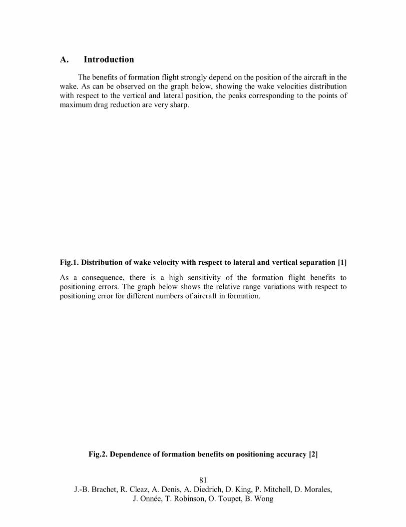
The benefits of formation flight strongly depend on the position of the aircraft in the wake. As can be observed on the graph below, showing the wake velocities distribution with respect to the vertical and lateral position, the peaks corresponding to the points of maximum drag reduction are very sharp.
Fig.1. Distribution of wake velocity with respect to lateral and vertical separation [1]
As a consequence, there is a high sensitivity of the formation flight benefits to positioning errors. The graph below shows the relative range variations with respect to positioning error for different numbers of aircraft in formation.
Fig.2. Dependence of formation benefits on positioning accuracy [2]
81 J.-B. Brachet, R. Cleaz, A. Denis, A. Diedrich, D. King, P. Mitchell, D. Morales,
J. Onnée, T. Robinson, O. Toupet, B. Wong
This shows the importance of accurate position sensing. Uncertainties of the vortex transport on the order of 20 ft on the optimal separations result in a 50% decrease in formation flight benefits. Hence there is a need for a control system that does not rely only on theoretical models for the positioning but also takes advantage of the current flight data to lead the aircraft towards the optimum.
B. Architecture
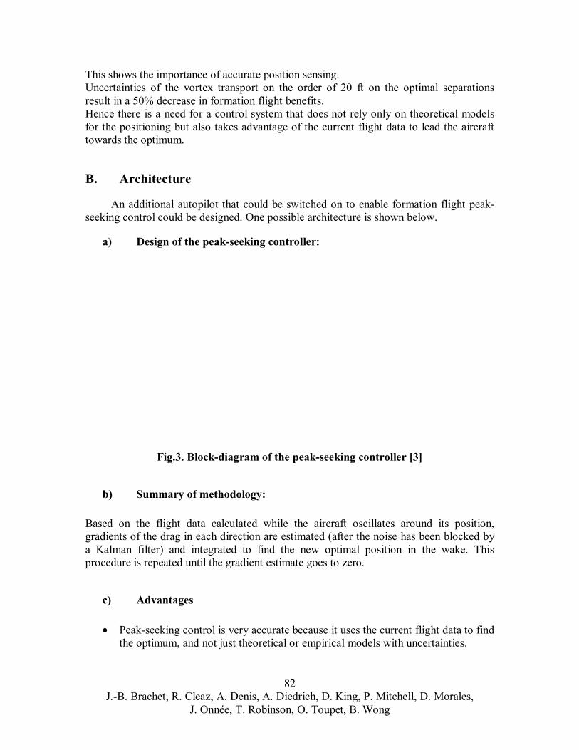
An additional autopilot that could be switched on to enable formation flight peak-seeking control could be designed. One possible architecture is shown below.
a) Design of the peak-seeking controller:
Fig.3. Block-diagram of the peak-seeking controller [3]
b) Summary of methodology:
Based on the flight data calculated while the aircraft oscillates around its position, gradients of the drag in each direction are estimated (after the noise has been blocked by a Kalman filter) and integrated to find the new optimal position in the wake. This procedure is repeated until the gradient estimate goes to zero.
c) Advantages
• Peak-seeking control is very accurate because it uses the current flight data to find the optimum, and not just theoretical or empirical models with uncertainties.
82 J.-B. Brachet, R. Cleaz, A. Denis, A. Diedrich, D. King, P. Mitchell, D. Morales,
J. Onnée, T. Robinson, O. Toupet, B. Wong
• This type of controller is much less dependent on the model. Hence the controller should fit a large range of aircraft without having to make any modifications.
• The optimization is very precise and fast-converging thanks to the use of a gradient search technique.
d) Disadvantages
• There is additional fatigue due to the need of oscillating around the flight path to search for better locations.
• Peak-seeking control for formation flight is technically challenging and still at the simulation stage.
• The aircraft can be trapped at local drag minima because it performs a gradient-based search. This is especially significant for performance in clear air turbulence (CAT) since the upwash field contains several transient local maxima.
C. Conclusion
A possible solution would be to use station-keeping control to get close to the optimal location (avoid the local minima) and then use extremum-seeking control to get and stay at the optimal with great precision.
83 J.-B. Brachet, R. Cleaz, A. Denis, A. Diedrich, D. King, P. Mitchell, D. Morales,
J. Onnée, T. Robinson, O. Toupet, B. Wong

References
[1] Kartik B. Ariyur and Miroslav Krsti , 2003, “Real-Time Optimization by Extremum-Seeking Control”, Wiley-Interscience, pp.119-141.
[2] William Blake and Dieter Multhopp, “Design Performance and Modeling Considerations for Close Formation Flight”, Air Force Research Laboratory, Wright Patterson AFB, Ohio, AIAA-98-4343.
[3] D. F. Chichka and J. L. Speyer, University of California, Los Angeles, California, and C. G. Park, Kwangwoon University, Seoul, Korea, “Peak-seeking Control with Application to Formation Flight”.
84 J.-B. Brachet, R. Cleaz, A. Denis, A. Diedrich, D. King, P. Mitchell, D. Morales,
J. Onnée, T. Robinson, O. Toupet, B. Wong

85 J.-B. Brachet, R. Cleaz, A. Denis, A. Diedrich, D. King, P. Mitchell, D. Morales,
J. Onnée, T. Robinson, O. Toupet, B. Wong

IX. Position and Velocity Estimation & Intra-
formation Communications
86 J.-B. Brachet, R. Cleaz, A. Denis, A. Diedrich, D. King, P. Mitchell, D. Morales,
J. Onnée, T. Robinson, O. Toupet, B. Wong
A. Introduction
This appendix outlines the different technologies considered for the subsystems in the autonomous formation flight system that handle position and velocity estimation for station-keeping, and intra-formation communications. There are three main sections to this part of the document. The first deals with position and velocity estimation, the second with mediums for intra-formation communications, and the third with communications topologies. In each section, subsystem requirements are presented, followed by background about each technology. Finally tables comparing the different technologies are displayed along with the selected technology.
Further information in this appendix includes an available data-rate calculation. Information about system architecture selection is contained within another appendix: Architecture Selection.
B. Position and Velocity Estimation
In order to support the station-keeping algorithm of the control system, a sensing system is needed to determine the relative position and velocity of each aircraft with respect to other aircraft in the formation. Various technologies are potentially available for estimating position and velocity. For the formation flight system, position needs to be accurate to within 0.1 wingspans of the ideal “sweet spot” in order to achieve maximum drag-reduction benefits. This translates to a required control accuracy of 12.5 ft for a B757-300, the smallest aircraft for which substantial benefits could be realized from formation flight. As a rule of thumb, sensing accuracy should be an order of magnitude better than the control accuracy, and so the goal for the position and velocity estimation system was to have a position accuracy of at least 15 in. Likewise, the velocity estimation accuracy goal was to be within 15 in/s or 1.25 ft/s.
The key issues in the evaluation of technologies for position and velocity estimation include:
i. required accuracy and range observed in similar applications ii. need for unobstructed path between measurement device and target iii. development and certification risk, which is broken into:
a. ease of certification due to demonstrated results from related applications b. safety
iv. dependence on intra-formation communications v. dependence on external systems vi. possibility of producing interference with internal and external systems vii. susceptibility to interference from internal and external systems including
weather conditions There are other issues to be considered as well such as complexity and the amount
of physical space a system will occupy on the aircraft. However, such issues are omitted
87 J.-B. Brachet, R. Cleaz, A. Denis, A. Diedrich, D. King, P. Mitchell, D. Morales,
J. Onnée, T. Robinson, O. Toupet, B. Wong
from this analysis either because of quantification difficulties, as in the case of complexity, or secondary importance, as in the case of physical space.
Tradeoffs in the evaluation of technologies for position and velocity estimation include:
i. increased accuracy vs. increased cost ii. increased accuracy vs. increased development risk (for new technologies)
Technologies that were considered for position and velocity estimation are listed below.
a) Carrier-phase Differential GPS and IMU Differential GPS typically uses a stationary base-station in a known location to
calculate the measurement errors from different GPS satellites. Since the distances to be measured between aircraft are small compared to the distance to the GPS satellites, the signals can be assumed to have traveled through the same “slice” of atmosphere and therefore have virtually the same errors. These measurements are then sent to moving receivers.1 In the case of formation flight, the base-station is also moving, thus the relative error is calculated instead of absolute error, and the accuracy is on the order of 10 to 20 feet (3 to 6 meters) using code-phase GPS.
For further accuracy, carrier-phase GPS can be used instead of “regular” code-phase GPS. Code-phase GPS receivers attempt to determine the time delay of a GPS satellite signal by matching up the pseudo-random code from the satellite with a pseudo-random code that it is generating. Since the pseudo-random code has a cycle width of almost a microsecond, this translates to a maximum of almost 1000 ft (300 meters) of error.1 However, good receivers can have an accuracy of 10 to 20 feet (3 to 6 meters) as stated above.
Carrier-phase GPS attempts to match the 1.57 GHz GPS signal, which has a wavelength of about 8 inches (20 centimeters). This translates to an accuracy of up to 0.10 to 0.15 inches (3 to 4 millimeters).1 A carrier-phase GPS receiver first uses code-phase GPS to achieve as much accuracy as possible and then improves it by matching the carrier signal.
Using a combination of carrier-phase and differential GPS-enhancement methods, the accuracy of relative position can theoretically be improved to within a few inches. In practice, NASA Dryden’s autonomous formation flight experiments found the achievable accuracy of such a system to be within 1 foot when filtered with IMU data.2 This 1-foot accuracy is within the 15 in requirement stated above for the formation flight system. Relative velocity can be estimated by taking several measurements over a period of time.
In the method outlined above, each aircraft in the formation would calculate its own relative states and send this information back to the leader, which would in turn send control commands to each aircraft. Alternatively, inverted DGPS could be used, whereby
88 J.-B. Brachet, R. Cleaz, A. Denis, A. Diedrich, D. King, P. Mitchell, D. Morales,
J. Onnée, T. Robinson, O. Toupet, B. Wong
each aircraft would send its uncorrected GPS location to the leader, which would centrally calculate the more precise relative positions of each aircraft.1
An inertial measurement unit (IMU) uses gyros and accelerometers to measure the angular rates and accelerations of an aircraft. By employing an IMU in the same manner as was used on NASA Dryden’s autonomous formation flight experiments, it can not only determine the angular rates and accelerations for an aircraft in three orthogonal axes, but also help to improve GPS data for better estimates of relative position. The improved estimates are generated by combining the output of the IMU with GPS data using a Kalman filter.3,4 These calculations would be performed by a processor in the position and velocity estimation unit. The GPS and IMU measurements can then be passed on to the leader aircraft for use in the control algorithm.
b) Lidar or Laser Radar Lidar or laser radar can be used to determine the distance from an object. In a lidar
system, a laser generates optical pulses and a receiver measures the time it takes for the pulse to be reflected back to the source.5 Multiplying this delay by the speed of light gives twice the distance to the object as the pulse must travel to the object and back. Making multiple measurements over a period of time allows velocity to be estimated in addition to position. Alternatively, lidar data could be combined with IMU measurements to improve accuracy in a manner similar to the one described above for GPS data. In some areas, lidar guns are used by police in speed traps in the same way as radar guns. Used in conjunction with the reflective paint found on certain license plates, these police lidar guns can have ranges of up to 2500 ft.6 Using reflective paint on certain known points on the aircraft will not only increase range, but also allow aircraft attitude to be determined by tracking the relative movement of those points with a laser. It is also conceivable to use a single laser system for both measurement and communications, although this has not yet been attempted.
c) Laser scanner Laser scanners are often used to determine three-dimensional geometry. One type
of commonly used laser scanning system uses a laser to shine a stripe of light onto an object and a camera to observe the geometry of that stripe as it sweeps across the surface of the object. Using mirrors, multiple virtual camera angles can be used to achieve a more complete scan of the object as certain areas may not be visible from certain angles.7The resulting 3D capture would potentially allow the attitude of an aircraft to be determined. However, it would be difficult to achieve the required amount of detail for attitude estimation in real time for a moving object being measured from a moving platform. The amount of calibration and re-calibration needed would be extremely high. Thus, a laser scanner would probably not be a viable option for position or velocity estimation for the formation flight system.
89 J.-B. Brachet, R. Cleaz, A. Denis, A. Diedrich, D. King, P. Mitchell, D. Morales,
J. Onnée, T. Robinson, O. Toupet, B. Wong
d) Optical Camera An optical camera can be used as part of a lidar or laser scanning system to
determine the distance to an object. It can also be used without a laser to track a moving target, provided that the target has been modified to allow the camera to easily “see” it. One possibility would be to combine an image sensor and a processing unit into a DSP camera that would track visual markings on an adjacent aircraft. By tracking the changes in size and shape of the markings due to changes in viewing angle using brightness levels in grey-scale images, the distance to the target as well as the relative attitude of the aircraft could be determined. A visual system for tracking cars was described by Marmoiton et al. at the IEEE Intelligent Vehicles Symposium in 2000.8 This system, mounted on a moving vehicle, was able to track two targets in real time (40 ms delay) by analyzing 25 images per second. An example of relative speed estimation at a distance of 25 m was also described, with a minimum error of 3.6% at 50 km/h and a maximum error of 9.8% at 80 km/h. Although it seems possible that a more refined version of the system would be able to achieve the necessary accuracy for the formation flight system, the car-tracking system as it stands has errors which are too large for accurate estimation as a stand alone system. However, Marmoiton et al. do mention the possibility of coupling the system with GPS to improve tracking, and the differences in tracking method as compared to other technologies make the optical camera a good candidate for a back-up collision avoidance system. As an example of the potential for this system, an optical camera measurement system was used in a joint Volpe-MIT study on aircraft noise attenuation, where two cameras on the ground were used to track aircraft flying overhead.9 Although the recognition was done using a different method called pixel tracking and the processing was not done in real-time, the use of this system shows that an optical camera system has the potential to be used at the distances required for aircraft.
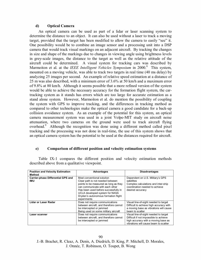
e) Comparison of different position and velocity estimation systems
Table IX-1 compares the different position and velocity estimation methods described above from a qualitative viewpoint.
Position and Velocity Estimation Method
Advantages Disadvantages
Carrier-phase Differential GPS and IMU
Most conventional solution Clear path is not needed between points to be measured as long as they can communicate with each other Has been used before successfully in UCLA developed system for NASA Dryden’s autonomous formation flight experiments
Dependent on U.S. Military’s GPS satellites Complex calculations and inter-ship coordination needed to achieve desired accuracy
Lidar or Laser Radar Does not require communications between aircraft, and therefore cannot be intercepted or jammed Being used on some military aircraft
Visual line-of-sight needed to target Difficult to achieve high accuracy with a moving base as vibrations will cause beam to scatter
Laser scanner Does not require communications between aircraft, and therefore cannot be intercepted or jammed
Visual line-of-sight needed to target Difficult if not impossible to achieve high accuracy with a moving base as vibrations will cause beam to scatter
90 J.-B. Brachet, R. Cleaz, A. Denis, A. Diedrich, D. King, P. Mitchell, D. Morales,
J. Onnée, T. Robinson, O. Toupet, B. Wong
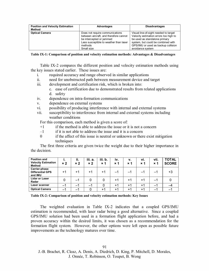
Position and Velocity Estimation Advantages Disadvantages Method Optical Camera Does not require communications Visual line-of-sight needed to target
between aircraft, and therefore cannot Velocity estimation errors too high to be intercepted or jammed be used as standalone primary Less susceptible to weather than laser system, but could be combined with methods GPS/IMU or used as backup collision Small size avoidance system
Table IX-1: Comparison of position and velocity estimation methods: Advantages & Disadvantages
Table IX-2 compares the different position and velocity estimation methods using the key issues stated earlier. These issues are:
i. required accuracy and range observed in similar applications ii. need for unobstructed path between measurement device and target iii. development and certification risk, which is broken into:
c. ease of certification due to demonstrated results from related applications d. safety
iv. dependence on intra-formation communications v. dependence on external systems vi. possibility of producing interference with internal and external systems vii. susceptibility to interference from internal and external systems including
weather conditions For this comparison, each method is given a score of: +1 if the method is able to address the issue or it is not a concern –1 if it is not able to address the issue and it is a concern 0 if the affect of this issue is neutral or unknown or there exist mitigation
techniques The first three criteria are given twice the weight due to their higher importance in
the decision.
Position and Velocity Estimation Method
i.× 2
ii.× 2
iii. a. × 2
iii. b. × 1
iv. × 1
v.× 1
vi. × 1
vii. × 1
TOTAL SCORE
Carrier-phase Differential GPS and IMU
+1 +1 +1 +1 –1 –1 –1 –1 +3
Lidar or Laser Radar 0 –1 0 0 +1 +1 +1 –1 0Laser scanner –1 –1 –1 0 +1 +1 +1 –1 –4Optical Camera –1 –1 0 +1 +1 +1 +1 –1 –1
Table IX-2: Comparison of position and velocity estimation methods: Key Issues
The weighted evaluation in Table IX-2 indicates that a coupled GPS/IMU estimation is recommended, with laser radar being a good alternative. Since a coupled GPS/IMU solution had been used in a formation flight application before, and had a proven accuracy within the desired limits, it was chosen as a recommendation for the formation flight system. However, the other options were left open as possible future improvements as the technology matures over time.
91 J.-B. Brachet, R. Cleaz, A. Denis, A. Diedrich, D. King, P. Mitchell, D. Morales,
J. Onnée, T. Robinson, O. Toupet, B. Wong
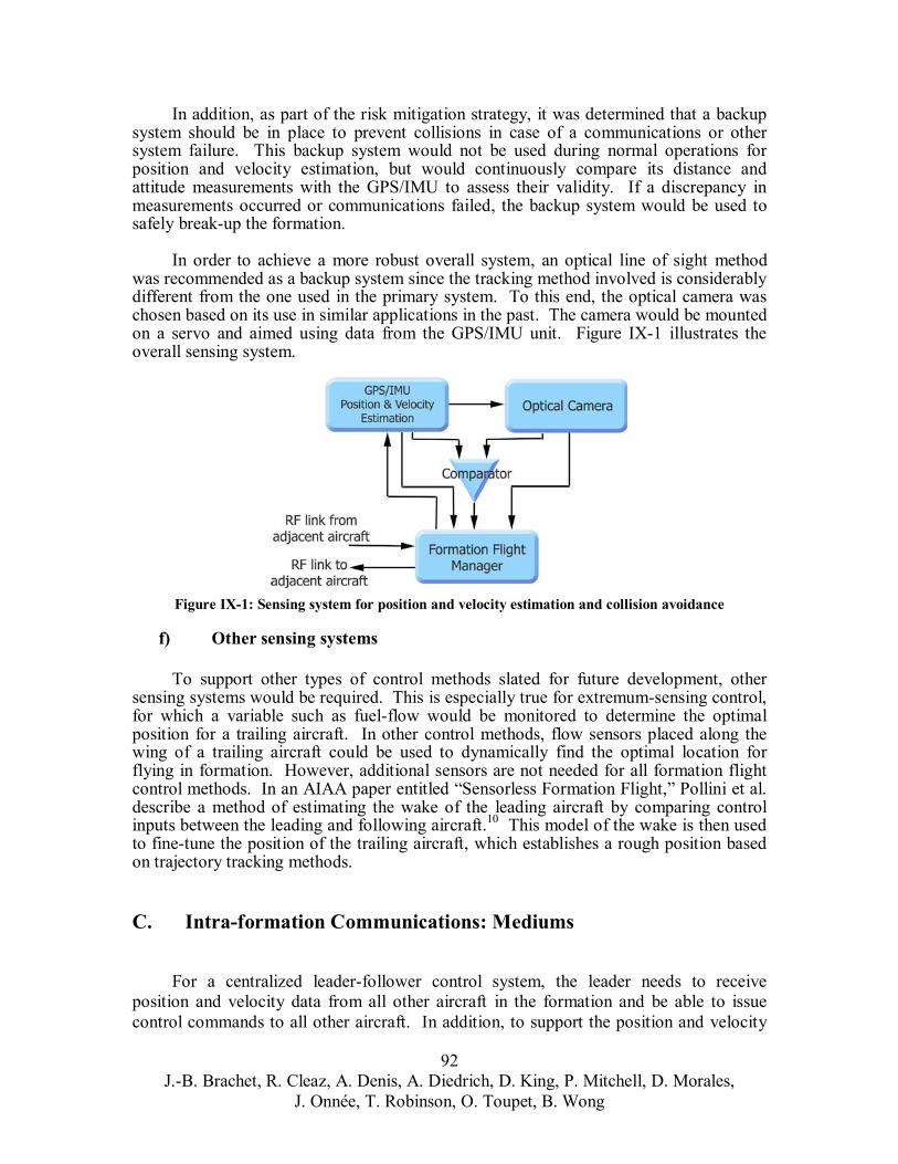
In addition, as part of the risk mitigation strategy, it was determined that a backup system should be in place to prevent collisions in case of a communications or other system failure. This backup system would not be used during normal operations for position and velocity estimation, but would continuously compare its distance and attitude measurements with the GPS/IMU to assess their validity. If a discrepancy in measurements occurred or communications failed, the backup system would be used to safely break-up the formation.
In order to achieve a more robust overall system, an optical line of sight method was recommended as a backup system since the tracking method involved is considerably different from the one used in the primary system. To this end, the optical camera was chosen based on its use in similar applications in the past. The camera would be mounted on a servo and aimed using data from the GPS/IMU unit. Figure IX-1 illustrates the overall sensing system.
Figure IX-1: Sensing system for position and velocity estimation and collision avoidance
f) Other sensing systems
To support other types of control methods slated for future development, other sensing systems would be required. This is especially true for extremum-sensing control, for which a variable such as fuel-flow would be monitored to determine the optimal position for a trailing aircraft. In other control methods, flow sensors placed along the wing of a trailing aircraft could be used to dynamically find the optimal location for flying in formation. However, additional sensors are not needed for all formation flight control methods. In an AIAA paper entitled “Sensorless Formation Flight,” Pollini et al. describe a method of estimating the wake of the leading aircraft by comparing control inputs between the leading and following aircraft.10 This model of the wake is then used to fine-tune the position of the trailing aircraft, which establishes a rough position based on trajectory tracking methods.
C. Intra-formation Communications: Mediums
For a centralized leader-follower control system, the leader needs to receive position and velocity data from all other aircraft in the formation and be able to issue control commands to all other aircraft. In addition, to support the position and velocity
92 J.-B. Brachet, R. Cleaz, A. Denis, A. Diedrich, D. King, P. Mitchell, D. Morales,
J. Onnée, T. Robinson, O. Toupet, B. Wong
estimation system, DGPS error correction factors need to be sent from the leader to all trailing aircraft. In order to accomplish this, a wireless network must be implemented within the formation. It is assumed that digital communications will be used instead of analog communications because of a wide range of benefits including:
i. more efficient use of bandwidth ii. possibility of encryption iii. lower average transmitter power due to efficiency iv. smaller receivers and transmitters
Although the type of airborne, wireless network required by autonomous flight has never been implemented, it is currently a hot research topic in the communications field, and there are several related technologies that could be adapted for such use. In the sections that follow are some of the most promising technologies.
The key issues in the evaluation of technologies for intra-formation communications mediums include:
i. required range observed in similar applications ii. required data rate observed in similar applications (includes propagation
delays). An available data rate calculation is computed in a later section of this appendix.
iii. susceptibility to turbulence in an airborne environment iv. development and certification risk, or ease of certification due to
demonstrated results from related applications v. line of sight needed vi. dependence on external systems vii. possibility of producing interference with internal and external systems viii. susceptibility to interference from internal and external systems including
weather conditions ix. limited use due to regulations or the FCC and other authorities
Tradeoffs in the evaluation of technologies for intra-formation communications mediums include:
i. increased quality of signal vs. increased delay ii. increased quality of signal vs. decreased bandwidth due to increased overhead
used for error checking and other quality improvements iii. increased range vs. increased power required
a) Radio-frequency (RF) communications
This is the most standard method of communications used today for similar wireless applications. The advantages to using radio communications include having proven systems currently in use and the resulting low cost to implement radio-frequency communications. The main disadvantages are also due to the high popularity of radio communications. These include the possibility of interference with other equipment on and off the aircraft, and the number of regulations governing the use of radio frequencies that vary from region to region.
93 J.-B. Brachet, R. Cleaz, A. Denis, A. Diedrich, D. King, P. Mitchell, D. Morales,
J. Onnée, T. Robinson, O. Toupet, B. Wong
Use of radio frequencies can be requested from the FCC and equivalent regulatory agencies in other countries. Using a chart of the radio frequency spectrum and a copy of FCC frequency allocations, possible choices for frequencies can be selected.11,12 These may lie in regulated or unregulated (amateur) bands. It is likely that the selected frequencies for autonomous formation flight communications will be microwaves in the UHF and SHF bands, similar to Wi-Fi technology currently in use for wireless network applications, or be in the HF band, similar to other aeronautical communications. Different frequency ranges have different characteristics; however, regular 802.11 Wi-Fi speeds have been achieved over distances of eight to ten miles using commercial solutions.13 This translates to data rates of 11 Mbps using the 802.11b standard, and 54 Mbps using the 802.11a or 802.11g standards. The new 802.16 standard for wireless communications could bring data rates of up to 70 Mbps. In addition, an IEEE workgroup is developing a new standard, 802.20, whose goal is to “optimize IP-based data transport, target peak data rates per user at over 1 Mbit/sec, and support vehicular mobility up to 250 km/hour.”14 With the combination of new technologies and a trusted medium, radio wireless communications seem like a viable option. Below are different types of wireless radio frequency channels, or propagation methods.
b) Line of sight
Most radio communications require a clear line of sight between the transmitter and receiver. In addition to a visual line-of-sight, an elliptical Fresnel Clearance Zone must be available. As a result line of sight radio communications would only be available between aircraft that could “see” each other in formation, and information to other aircraft would have to be relayed. Note that although signal components can be reflected by the ground in radio communications, these signal components are generally regarded as a problem requiring mitigation since signal components reflected by the ground generally arrive at the receiver with different delays and attenuations and are not particularly useful.15 However, as listed below, there are other ways in which radio waves can be reflected around an obstacle such as an aircraft.
c) High Frequency band reflected by the ionosphere
If frequencies in the HF band are used for RF communications, they can be reflected by layers of the ionosphere. Thus, non-adjacent aircraft in the formation would be able to communicate directly with each other without having the relay the signal through another aircraft. Unfortunately, the HF band is crowded with high usage, and the refraction causes signal components to have different offsets, causing signal fading and reduced quality.15 On the bright side, there exist tried and true methods for resolving multipath signal components using direct-sequence spread spectrum techniques.
94 J.-B. Brachet, R. Cleaz, A. Denis, A. Diedrich, D. King, P. Mitchell, D. Morales,
J. Onnée, T. Robinson, O. Toupet, B. Wong
d) Satellite relay
Another method of avoiding line-of-sight blockages is to use a satellite to relay the signal. However, these satellite links would have a delay of about half a second, which could be too long for the control system.16 Using a satellite relay also has the disadvantage of having to rely on one or more satellites.
e) Optical or Infrared Laser Communications
In addition to measuring distance, pulses of visible or infrared laser light can be used to send information.17 These free-space laser communications systems are primarily used to send data between stationary buildings and as satellite communications crosslinks, although some military aircraft are also equipped for lasercom. They are similar in nature to fiber optic systems except that they travel through the atmosphere or through space instead of along optical fibers. The maximum range available for commercial inter-building applications is around 3 miles, and the data rates achievable are 155 Mbps.18 With a moving link, the data rate would probably be somewhat lower due to additional error correction needed in a vibrating environment and having to re-establish the link as aircraft shift in relative position. In 2002, the U.S. Naval Research Laboratory established a free-space laser communication link across Chesapeake Bay that spanned 16.2 km; however, this system used a high-power laser that would be unsuitable for airborne wireless communications.19
The advantages to using a laser link include low observability and the lack of interference with RF systems. Lasercom also uses a third to half of the power required for an RF link with equivalent data rate, and transceivers typically weigh only 40-45% of an equivalent RF system. In addition, it is difficult to jam lasercom, or at least jamming is instantly detectable due to the reduction in beam intensity from splitting off part of the beam.20 Disadvantages of lasercom include difficulties in aiming a beam in a vibrating environment, saturation of the receiver from sunlight, and scattering of the beam due to fog and other precipitation.21 However, various mitigation techniques have been developed to minimize the effects of atmospheric conditions. These include using various coding schemes in addition to simply increasing the power of the laser beam.22 It is also possible to use a concept known as omni-directional laser communications to decrease aiming problems. With this concept, pulses from the transmitting laser are split into multiple parallel beams that are all sent in the general direction of the recipient aircraft’s receiver. The recipient aircraft is also equipped with multiple identical receivers. In this manner it is likely that at least one transmitter and receiver pair will line up at all times and data will be received. A study on omni-directional laser communications conducted at the Chang Chun Institute of Optics and Fine Mechanic found that such a system had a range of 3 km.23 One of the additional downsides to a single laser beam is the inability to carry out 1:N communications simultaneously. Luckily, mirrors and beam-splitters can be used to send data to multiple recipients.
95 J.-B. Brachet, R. Cleaz, A. Denis, A. Diedrich, D. King, P. Mitchell, D. Morales,
J. Onnée, T. Robinson, O. Toupet, B. Wong
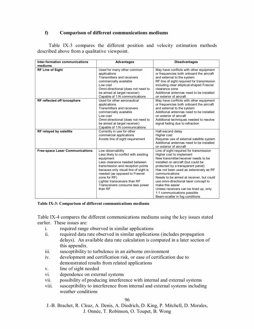
f) Comparison of different communications mediums
Table IX-3 compares the different position and velocity estimation methods described above from a qualitative viewpoint.
Inter-formation communications mediums
Advantages Disadvantages
RF Line of Sight Used for many other common applications Transmitters and receivers commercially available Low cost Omni-directional (does not need to be aimed at target receiver) Capable of 1:N communications
May have conflicts with other equipment or frequencies both onboard the aircraft and external to the system RF line of sight required for transmission including clear elliptical-shaped Fresnel clearance zone Additional antennas need to be installed on exterior of aircraft
RF reflected off Ionosphere Used for other aeronautical applications Transmitters and receivers commercially available Low cost Omni-directional (does not need to be aimed at target receiver) Capable of 1:N communications
May have conflicts with other equipment or frequencies both onboard the aircraft and external to the system Additional antennas need to be installed on exterior of aircraft Additional techniques needed to resolve signal fading due to refraction
RF relayed by satellite Currently in use for other commercial applications Avoids line of sight requirement
Half-second delay Higher cost Requires use of external satellite system Additional antennas need to be installed on exterior of aircraft
Free-space Laser Communications Low observability Less likely to conflict with existing equipment Less clearance needed between transmission and reception points because only visual line of sight is needed (as opposed to Fresnel zone for RF) Lighter transceivers than RF Transceivers consume less power than RF
Line of sight required for transmission Higher cost to implement New transmitter/receiver needs to be installed on aircraft (but could be protected by a transparent panel) Has not been used as extensively as RF communications Needs to be aimed at receiver, but could use omni-directional laser concept to make this easier Unless receivers can be lined up, only 1:1 communications possible Beam-scatter in fog conditions
Table IX-3: Comparison of different communications mediums
Table IX-4 compares the different communications mediums using the key issues stated earlier. These issues are:
i. required range observed in similar applications ii. required data rate observed in similar applications (includes propagation
delays). An available data rate calculation is computed in a later section of this appendix.
iii. susceptibility to turbulence in an airborne environment iv. development and certification risk, or ease of certification due to
demonstrated results from related applications v. line of sight needed vi. dependence on external systems vii. possibility of producing interference with internal and external systems viii. susceptibility to interference from internal and external systems including
weather conditions
96 J.-B. Brachet, R. Cleaz, A. Denis, A. Diedrich, D. King, P. Mitchell, D. Morales,
J. Onnée, T. Robinson, O. Toupet, B. Wong
ix. limited use due to regulations made by FCC and other certifying authorities For this comparison, each method is given a score of: +1 if the method is able to address the issue or it is not a concern –1 if it is not able to address the issue and it is a concern 0 if the affect of this issue is neutral or unknown or there exist mitigation
techniques The first four criteria are given twice the weight due to their higher importance in
the decision.
Intra-formation communications mediums
i.× 2
ii.× 2
iii. × 2
iv. × 2
v.× 1
vi. × 1
vii. × 1
viii. × 1
ix. × 1
TOTAL SCORE
RF Line of Sight +1 +1 +1 +1 –1 +1 –1 0 –1 +6RF reflected off Ionosphere +1 +1 +1 +1 +1 +1 –1 0 –1 +8RF relayed by satellite +1 –1 +1 +1 +1 –1 –1 0 –1 +2 Free-space Laser Communications +1 +1 –1 0 –1 +1 +1 0 +1 +4
Table IX-4: Comparison of different communications mediums: Key Issues
Based on the familiarity of radio frequency communications, the omni-directional capabilities and lower cost, radio frequency communications were chosen as the currently preferred method for intra-formation communications, while leaving open the possibility of using laser communications in the future as the technology matures. With RF communications, either a line-of-sight or HF solution may be possible depending on approval from the FCC, the ETSI and other regulatory authorities. Since approval is not guaranteed at this point, further sections on communications architecture assume that a line of sight is required for communications, as HF may not be available. Even HF will have better propagation if a line of sight is available.
D. Intra-formation Communications: Network Structures
a) Physical Network Topology
Depending on the formation shape, various physical network architectures are available. The physical architecture is a plan of how the formation flight managers of the aircraft in formation are connected to each other and how they relay information. Although the choices of network topology are infinite for a wireless network due to the lack of physical connections, the main choice for the formation flight system centered around two topologies that preserved symmetry given the limitations set by the formation shape and the necessity for rotation, which meant that any aircraft could be called upon to act as the leader and command-issuing nerve center of the formation. The first possible topology had all aircraft receiving information directly from all other aircraft. The second had aircraft only receiving information relayed through adjacent aircraft in the formation.
97 J.-B. Brachet, R. Cleaz, A. Denis, A. Diedrich, D. King, P. Mitchell, D. Morales,
J. Onnée, T. Robinson, O. Toupet, B. Wong
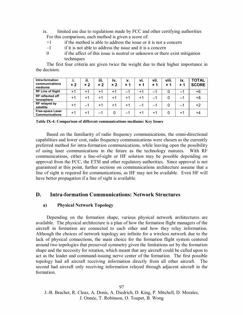
In order to optimize the formation, graph theory can be used to solve a shortest path problem using the Dijkstra algorithm with each aircraft being a node in the network and the connections between aircraft represented as arcs.24 This minimizes the number of links needed and the power needed to support those links. With an echelon formation shape, the problem becomes trivial as all aircraft are simply connected to their adjacent aircraft to achieve the shortest path (Figure IX-2).
Figure IX-2: Communications topology
Aircraft icon from http://www.cancer.dk/resources/ed3+airplane+icon.jpg
In the event of a communications failure, the network can be thought of as having lost the outgoing arcs from a particular node, in which case the new optimal configuration for an echelon formation would merely involve connecting the two nodes that were formerly connected to that node in order to heal the network.
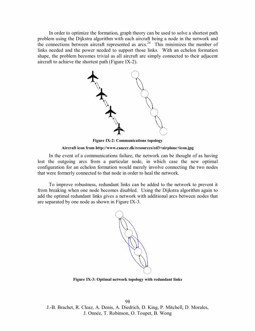
To improve robustness, redundant links can be added to the network to prevent it from breaking when one node becomes disabled. Using the Dijkstra algorithm again to add the optimal redundant links gives a network with additional arcs between nodes that are separated by one node as shown in Figure IX-3.
Figure IX-3: Optimal network topology with redundant links
98 J.-B. Brachet, R. Cleaz, A. Denis, A. Diedrich, D. King, P. Mitchell, D. Morales,
J. Onnée, T. Robinson, O. Toupet, B. Wong
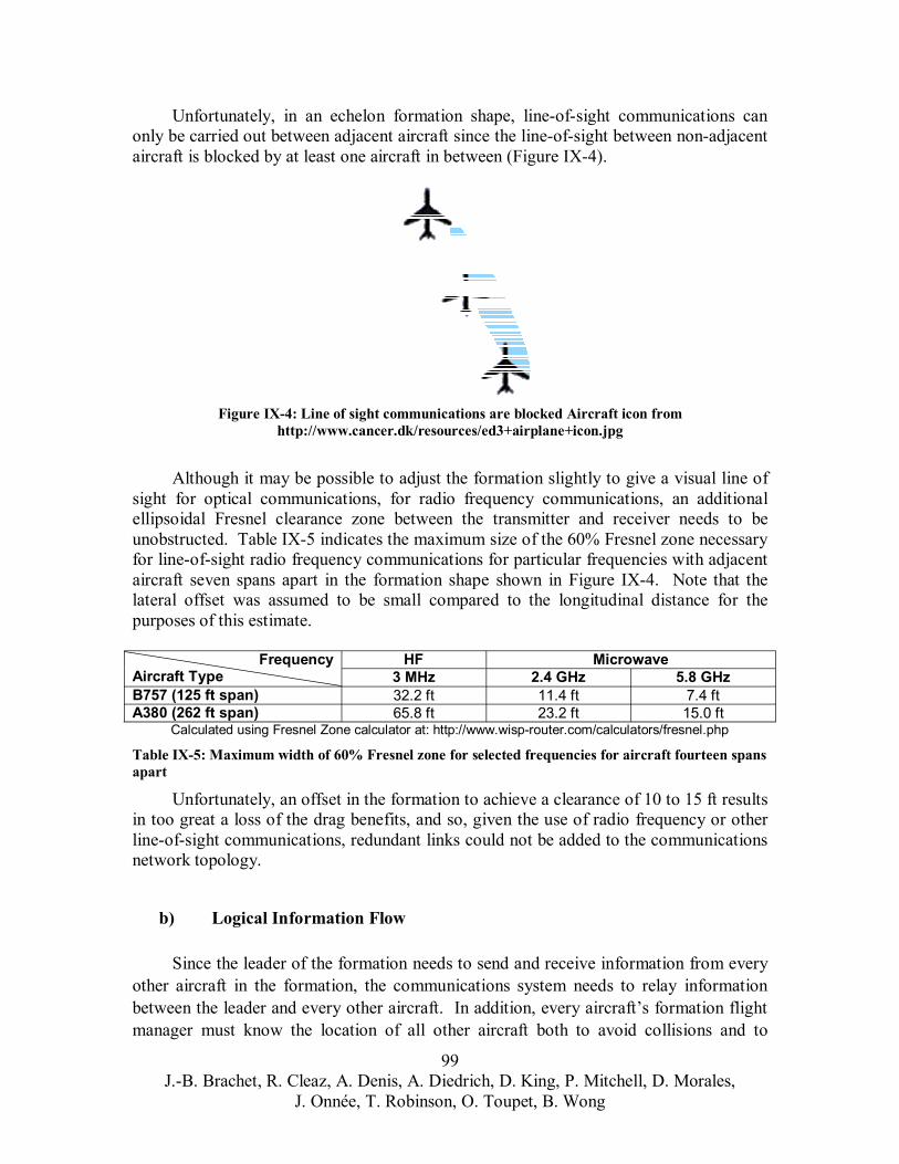
Unfortunately, in an echelon formation shape, line-of-sight communications can only be carried out between adjacent aircraft since the line-of-sight between non-adjacent aircraft is blocked by at least one aircraft in between (Figure IX-4).
Figure IX-4: Line of sight communications are blocked Aircraft icon from http://www.cancer.dk/resources/ed3+airplane+icon.jpg
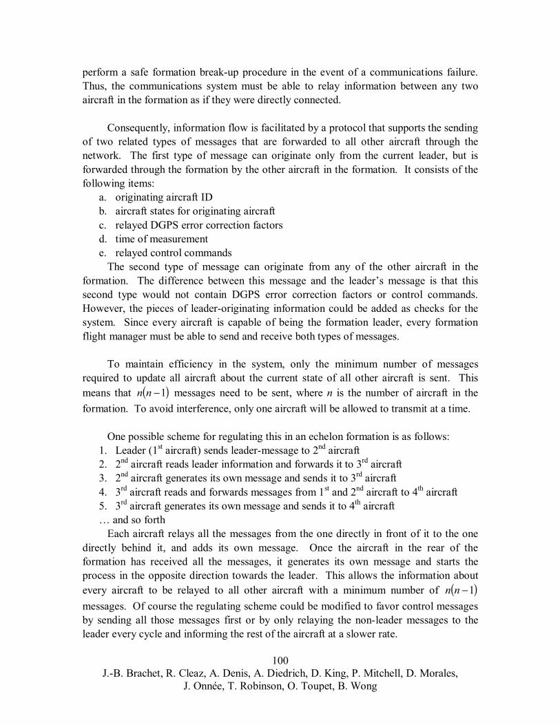
Although it may be possible to adjust the formation slightly to give a visual line of sight for optical communications, for radio frequency communications, an additional ellipsoidal Fresnel clearance zone between the transmitter and receiver needs to be unobstructed. Table IX-5 indicates the maximum size of the 60% Fresnel zone necessary for line-of-sight radio frequency communications for particular frequencies with adjacent aircraft seven spans apart in the formation shape shown in Figure IX-4. Note that the lateral offset was assumed to be small compared to the longitudinal distance for the purposes of this estimate.
Frequency Aircraft Type
HF Microwave 3 MHz 2.4 GHz 5.8 GHz
B757 (125 ft span) 32.2 ft 11.4 ft 7.4 ft A380 (262 ft span) 65.8 ft 23.2 ft 15.0 ft
Calculated using Fresnel Zone calculator at: http://www.wisp-router.com/calculators/fresnel.php
Table IX-5: Maximum width of 60% Fresnel zone for selected frequencies for aircraft fourteen spans apart
Unfortunately, an offset in the formation to achieve a clearance of 10 to 15 ft results in too great a loss of the drag benefits, and so, given the use of radio frequency or other line-of-sight communications, redundant links could not be added to the communications network topology.
b) Logical Information Flow
Since the leader of the formation needs to send and receive information from every other aircraft in the formation, the communications system needs to relay information between the leader and every other aircraft. In addition, every aircraft’s formation flight manager must know the location of all other aircraft both to avoid collisions and to
99 J.-B. Brachet, R. Cleaz, A. Denis, A. Diedrich, D. King, P. Mitchell, D. Morales,
J. Onnée, T. Robinson, O. Toupet, B. Wong
perform a safe formation break-up procedure in the event of a communications failure. Thus, the communications system must be able to relay information between any two aircraft in the formation as if they were directly connected.
Consequently, information flow is facilitated by a protocol that supports the sending of two related types of messages that are forwarded to all other aircraft through the network. The first type of message can originate only from the current leader, but is forwarded through the formation by the other aircraft in the formation. It consists of the following items:
a. originating aircraft ID b. aircraft states for originating aircraft c. relayed DGPS error correction factors d. time of measurement e. relayed control commands
The second type of message can originate from any of the other aircraft in the formation. The difference between this message and the leader’s message is that this second type would not contain DGPS error correction factors or control commands. However, the pieces of leader-originating information could be added as checks for the system. Since every aircraft is capable of being the formation leader, every formation flight manager must be able to send and receive both types of messages.
To maintain efficiency in the system, only the minimum number of messages required to update all aircraft about the current state of all other aircraft is sent. This
(means that n n − 1) messages need to be sent, where n is the number of aircraft in the formation. To avoid interference, only one aircraft will be allowed to transmit at a time.
One possible scheme for regulating this in an echelon formation is as follows: 1. Leader (1st aircraft) sends leader-message to 2nd aircraft 2. 2nd aircraft reads leader information and forwards it to 3rd aircraft 3. 2nd aircraft generates its own message and sends it to 3rd aircraft 4. 3rd aircraft reads and forwards messages from 1st and 2nd aircraft to 4th aircraft 5. 3rd aircraft generates its own message and sends it to 4th aircraft … and so forth
Each aircraft relays all the messages from the one directly in front of it to the one directly behind it, and adds its own message. Once the aircraft in the rear of the formation has received all the messages, it generates its own message and starts the process in the opposite direction towards the leader. This allows the information about
(every aircraft to be relayed to all other aircraft with a minimum number of n n − 1)messages. Of course the regulating scheme could be modified to favor control messages by sending all those messages first or by only relaying the non-leader messages to the leader every cycle and informing the rest of the aircraft at a slower rate.
100 J.-B. Brachet, R. Cleaz, A. Denis, A. Diedrich, D. King, P. Mitchell, D. Morales,
J. Onnée, T. Robinson, O. Toupet, B. Wong

E. Data-rate available
The following is a calculation of the data rate available from the communications system for a worst-case configuration where all aircraft receive information about all other aircraft.
Let each “message” contain data about one aircraft.
Assume 20 32-bit numbers need to be transmitted in each message to cover all data. This includes originating aircraft ID, up to 9 aircraft states, DGPS error correction factors for up to 5 satellites, time of measurement, and 4 control commands.
Now assume that any communications medium selected for formation flight has a minimum data rate of 3 Mbps or 3,000,000 bits per second. (Note: 220 bits is not correct in terms of communications data rates). This 3 Mbps can be thought of the data rate of 802.11b commercial Wi-Fi technology being degraded from 11 Mbps on the ground to 3Mbps due to long distances and high altitude.
(For n aircraft in formation, if only one can transmit at a time, n n − 1) messages must be sent within the entire system to update all aircraft with information about all other aircraft.
(Thus a total of 20× 32 × n n − 1) bits of information must be sent to update all (aircraft. Dividing by 3,000,000, this means that it takes about n n − 1) seconds to update 5000
for a full system update. The total update time is displayed in Table IX-6 for different numbers of aircraft in the formation.
Number of aircraft in 2 3 4 5 6 7 8 9 10formation Time for full system update
0.4 ms 1.2 ms 2.4 ms 4.0 ms 6.0 ms 8.4 ms 11.2 ms
14.4 ms
18.0 ms
Table IX-6: Time needed for full system update vs. number of aircraft in formation
These numbers indicate that the required data-update rate of 1-100 Hz for the control system can be met.
101 J.-B. Brachet, R. Cleaz, A. Denis, A. Diedrich, D. King, P. Mitchell, D. Morales,
J. Onnée, T. Robinson, O. Toupet, B. Wong

References
“All About GPS,” Trimble Navigation Limited, 2004. [http://www.trimble.com/gps/index.html. Accessed 5/9/04.]2 Cobleigh, B., “Capabilities and Future Applications of the NASA Autonomous Formation Flight (AFF) Aircraft,” AIAA Paper 2002-3443, AIAA’s 1st Conference and Workshop on Unmanned Aerospace Vehicles, Systems, Technologies and Operations, Portsmouth, VA, May 20-23, 2002. 3 Cobleigh, B., “Autonomous Formation Flight Project Phase 1 System Requirements Document,” Document No. AFF-PROJ-SRD-01.09, NASA Dryden Flight Research Center, Edwards, CA, November 5, 2001.4 Maybeck, P. S., Stochastic Models, Estimation and Control, Vol. 1, Academic Press, New York, 1979. 5 “About Laser Radar,” Optech Incorporated, 2003. [http://www.optech.on.ca/aboutlaser.htm. Accessed 5/9/04.]6 “Frequently Asked Questions on Police Lidar”, September 1, 1995. [http://www.mr2.com/TEXT/FAQonLidar.html. Accessed 5/9/04.]7 Davis, J., Chen, X., “A Laser Range Scanner Designed for Minimum Calibration Complexity,” Proceedings of the Third International Conference on 3D Digital Imaging and Modeling, 3DIM, IEEE Computer Society, Quebec City, May 28-June 1, 2001. 8 Marmoiton, F., Collange, F., Dérutin., J. P., “Location and relative speed estimation of vehicles by monocular vision,” Proceedings of the IEEE Intelligent Vehicles Symposium 2000, Dearborn, MI, October 3-5, 2000, pp. 227-232. 9 Senzig, D. A., Reherman, C. N., Roof, C. J., Fleming, G. G., “User’s Guide for Digital Video Tracking System,” DOT-34-VX005-LR-0X, U.S. Department of Transportation, Research and Special Programs Administration, John A. Volpe National Transportation Systems Center, Cambridge, MA, November, 2002.10 Pollini, L., Giulietti, F., Innocenti, M., “Sensorless Formation Flight,” AIAA Paper 01-4356, AIAA Guidance, Navigation, and Control Conference and Exhibit, American Institute of Aeronautics and Astronautics, Montreal, August 6-9, 2001. 11 “United States Frequency Allocations,” U.S. Department of Commerce, National Telecommunications and Information Administration, Office of Spectrum Management, March 1996. 12 “The FCC’s On-Line Table of Frequency Allocations,” Federal Communications Commission, Office of Engineering and Technology, Policy and Rules Division, April 13, 2004. [http://www.fcc.gov/oet/spectrum/table/fcctable.pdf. Accessed 5/14/04.]13 Stone, A., “Long Distance Wi-Fi,” Wi-Fi Planet, April 16, 2003. [http://www.wi-fiplanet.com/columns/article.php/2191841. Accessed 4/26/04.]14 Cohen, B., Deutsch, D., “802.16: The Future in Last Mile Wireless Connectivity,” CrossNodes,EarthWeb.com: The IT Industry Portal, Jupitermedia Corporation, August 18, 2003. [http://networking.earthweb.com/netsp/article.php/10953_3065261_2. Accessed 5/14/04.]15 Proakis, J. G., Salehi, M., “Wireless Communications,” Communications Systems Engineering, 2nd ed., Prentice Hall, Upper Saddle River, NJ, 2002, pp. 674-780. 16 Brown, J., “How Satellites Work,” HowStuffWorks, Inc. [http://electronics.howstuffworks.com/satellite7.htm. Accessed 5/10/04.]17 Lerner, E. J., “Optoelectronics and Laser Technology Advances,” Laser Focus World, June 2002. [http://cictr.ee.psu.edu/facstaff/kavehrad/Laser%20Focus%20World%20-%20Optoelectronics%20and%20Laser%20Technology%20Advances.htm. Accessed 4/26/04.]18 “FAQ AEI Wireless Communications,” AEI Warless Communications, 1999. [http://www.aeiwireless.com/html/faq.html. Accessed 4/26/04.]19 Moore, C. I., Burris, H. R., Suite, M. R., Stell, M. F., Vilcheck, M. J., Davis, M. A., Smith, R., Mahon, R., Rabinovich, W. S., Koplow, J., Moore, S. W., Scharpf, W. J., Reed, A. E., “Free-space high-speed laser communication link across the Chesapeake Bay,” Free-Space Laser Communication and Laser Imaging II,Proceedings of SPIE, The International Society for Optical Engineering, Vol. 4821, Seattle, WA, 2002, pp. 474-482. 20 Freidell, J. E., Brunt, P., Wilson, K. E., “Why laser communication crosslinks can’t be ignored,” 16th AIAA International Communications Satellite Systems Conference, American Institute of Aeronautics and Astronautics, Washington, DC, 1996, pp. 1397-1409.
102 J.-B. Brachet, R. Cleaz, A. Denis, A. Diedrich, D. King, P. Mitchell, D. Morales,
J. Onnée, T. Robinson, O. Toupet, B. Wong

[http://www.cms.livjm.ac.uk/pgnet2001/papers/mliu.doc. Accessed 4/26/04.] 21 Liu, M., Hill, S. L., “Free Space Point to Point Laser and Optical Communications,” Second Annual Network Symposium, School of Computing and Mathematical Sciences, Liverpool John Moores University, Liverpool, June 18-19 2001. [http://www.cms.livjm.ac.uk/pgnet2001/papers/mliu.doc. Accessed 4/26/04.] 22 Kiriazes, J. J., Phillips, R. L., Andrews, L. C., “Effects on pulse-position modulation for laser communication in the presence of atmospheric scintillation,” Free-Space Laser Communication and Laser Imaging I, Proceedings of the SPIE, The International Society for Optical Engineering, Vol. 4821, Seattle, WA, 2002, pp. 332-343. 23 Song, L., Wang, X., Hou, F., “Omni-directional digital laser communication system,” Optical Interconnects for Telecommunication and Data Communications, Proceedings of SPIE, The International Society for Optical Engineering, Vol. 4225, Beijing, November 8-10, pp. 220-222. 24 Giulietti, F., Pollini, L., Innocenti, M., “Autonomous Formation Flight,” IEEE Control Systems Magazine, Vol. 20, No. 6, December 2000, pp. 34-44.
103 J.-B. Brachet, R. Cleaz, A. Denis, A. Diedrich, D. King, P. Mitchell, D. Morales,
J. Onnée, T. Robinson, O. Toupet, B. Wong

X. Human Factors
104 J.-B. Brachet, R. Cleaz, A. Denis, A. Diedrich, D. King, P. Mitchell, D. Morales,
J. Onnée, T. Robinson, O. Toupet, B. Wong
The Appendix on Human Factors details the studies that have lead to defining the role pilots should play in the accomplishment of a formation flight. A closer look at the interface with the aircraft is then presented.
The goal of studying Human Factors is to help determine the role pilots will play formation flight. There are some main underlying questions to this issue:
• Are pilots needed on board these aircraft? • Are they needed in every plane? • What are their tasks? • What interface should be implemented between the pilot and the machine?
Several aspects help provide answers to these questions:
• The mission assigned to the aircraft. • Human capabilities from a physiological and cognitive point of view. • Socio-cultural and regulatory concerns. • Economic issues. • Architecture impact
Several possible pilot interfaces are outlined and the one retained for the system is described.
A. Impact of the Mission:
The need for a crew on board every aircraft is partly decided by the mission assigned to the cargo shipment.
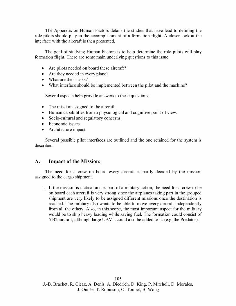
1. If the mission is tactical and is part of a military action, the need for a crew to be on board each aircraft is very strong since the airplanes taking part in the grouped shipment are very likely to be assigned different missions once the destination is reached. The military also wants to be able to move every aircraft independently from all the others. Also, in this scope, the most important aspect for the military would be to ship heavy loading while saving fuel. The formation could consist of 5 B2 aircraft, although large UAV’s could also be added to it. (e.g. the Predator).
105 J.-B. Brachet, R. Cleaz, A. Denis, A. Diedrich, D. King, P. Mitchell, D. Morales,
J. Onnée, T. Robinson, O. Toupet, B. Wong
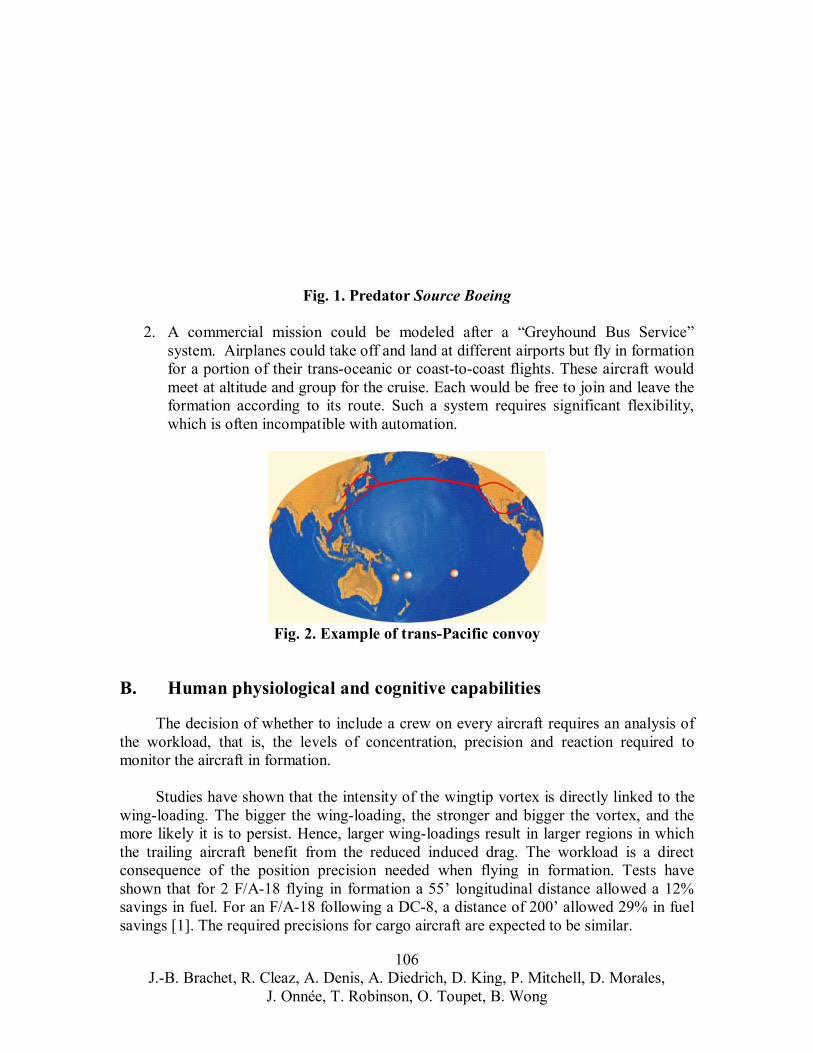
Fig. 1. Predator Source Boeing
2. A commercial mission could be modeled after a “Greyhound Bus Service” system. Airplanes could take off and land at different airports but fly in formation for a portion of their trans-oceanic or coast-to-coast flights. These aircraft would meet at altitude and group for the cruise. Each would be free to join and leave the formation according to its route. Such a system requires significant flexibility, which is often incompatible with automation.
Fig. 2. Example of trans-Pacific convoy
B. Human physiological and cognitive capabilities
The decision of whether to include a crew on every aircraft requires an analysis of the workload, that is, the levels of concentration, precision and reaction required to monitor the aircraft in formation.
Studies have shown that the intensity of the wingtip vortex is directly linked to the wing-loading. The bigger the wing-loading, the stronger and bigger the vortex, and the more likely it is to persist. Hence, larger wing-loadings result in larger regions in which the trailing aircraft benefit from the reduced induced drag. The workload is a direct consequence of the position precision needed when flying in formation. Tests have shown that for 2 F/A-18 flying in formation a 55’ longitudinal distance allowed a 12% savings in fuel. For an F/A-18 following a DC-8, a distance of 200’ allowed 29% in fuel savings [1]. The required precisions for cargo aircraft are expected to be similar.
106 J.-B. Brachet, R. Cleaz, A. Denis, A. Diedrich, D. King, P. Mitchell, D. Morales,
J. Onnée, T. Robinson, O. Toupet, B. Wong
Furthermore, the most significant effect at the maximum drag reduction position is a strong rolling moment.
Studies and flight experiments have shown that pilots have to capacity to fly in formation and maintain a good level of safety:
• Dedicated flight training strongly improves the skills and abilities of pilots to fly in formation. (Training Transfer of a Formation Flight Trainer by G.B.Reid, Air Force Human Resources Laboratory, 1975)
• Although uncommonly high, the level of reaction required by the vortex effects is within pilots’ capabilities. According to NASA’s study of Induced Moment Effects of Formation Flight Using two F/A-18 Aircraft (by J.L.Hansen & B.R.Cobleigh, NASA, August 2002): “[The] flight tests demonstrated that nearly all vortex-induced effects are easily compensable by the pilot. […] Although the vortex effects on the trailing edge were found to peak in the area of maximum drag reduction, these effects were well within the capability of the pilot.”
• The pilot of a trailing aircraft shows a time of reaction of 1 to 2 seconds to a modification of the trajectory of the airplane they are following. It may be significant that this study has been performed with Cessna aircraft, which are very different in terms of control commands and response time than traditional cargo carriers. Per “Visual, Cruise Formation Dynamics” (by S.Houck & J.D.Powell, Stanford University, 2000): “The […] analysis suggests that a pilot discerns bank angle change more quickly than either pitch or yaw angle changes. This response time averages about one second for separations less than 2000ft. Response to a climb maneuver is faster than that to a descent and is probably more natural response than pushing over in order to descend. Pilot response to a wings-level yaw maneuver is between one and five seconds, but frequently there is no response at all. This series of flight forms a basis for analyzing pilot response; however, additional issues such as individual differences in pilot response, differences in lead aircraft maneuver entry characteristics, and atmospheric factors such as sun angle, background terrain, and cloud coverage have not been addressed.”
In the meantime, there are some drawbacks to letting pilots fly cargo aircraft in formation:
• Pilots tend to overuse the throttle to adjust the position of their aircraft with respect to the leading airplane. The consequence is a slight increase in fuel consumption. Quoting from a NASA Study entitled “F/A-18 Performance Benefits Measured During the Autonomous Formation Flight Project” by M.J Vachon et al. in 2003: “The manually-flown trail airplane was also upset by the same gust and the pilot had to correct for large and dynamic variations in the separation distance from the lead airplane. To overcome this, the pilot greatly increased the frequency and amplitude of throttle movement to maintain proper separation. The result was that the trailing airplane actually measured more fuel use in the vortex than during the
107 J.-B. Brachet, R. Cleaz, A. Denis, A. Diedrich, D. King, P. Mitchell, D. Morales,
J. Onnée, T. Robinson, O. Toupet, B. Wong
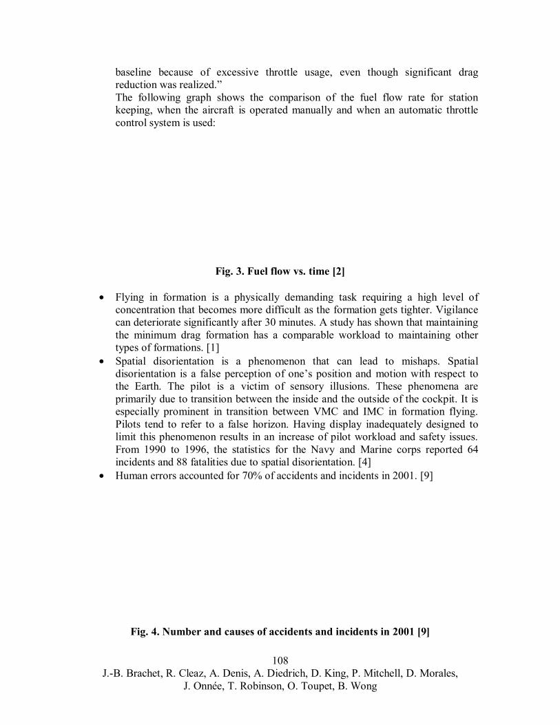
baseline because of excessive throttle usage, even though significant drag reduction was realized.” The following graph shows the comparison of the fuel flow rate for station keeping, when the aircraft is operated manually and when an automatic throttle control system is used:
Fig. 3. Fuel flow vs. time [2]
• Flying in formation is a physically demanding task requiring a high level of concentration that becomes more difficult as the formation gets tighter. Vigilance can deteriorate significantly after 30 minutes. A study has shown that maintaining the minimum drag formation has a comparable workload to maintaining other types of formations. [1]
• Spatial disorientation is a phenomenon that can lead to mishaps. Spatial disorientation is a false perception of one’s position and motion with respect to the Earth. The pilot is a victim of sensory illusions. These phenomena are primarily due to transition between the inside and the outside of the cockpit. It is especially prominent in transition between VMC and IMC in formation flying. Pilots tend to refer to a false horizon. Having display inadequately designed to limit this phenomenon results in an increase of pilot workload and safety issues. From 1990 to 1996, the statistics for the Navy and Marine corps reported 64 incidents and 88 fatalities due to spatial disorientation. [4]
• Human errors accounted for 70% of accidents and incidents in 2001. [9]
Fig. 4. Number and causes of accidents and incidents in 2001 [9]
108 J.-B. Brachet, R. Cleaz, A. Denis, A. Diedrich, D. King, P. Mitchell, D. Morales,
J. Onnée, T. Robinson, O. Toupet, B. Wong
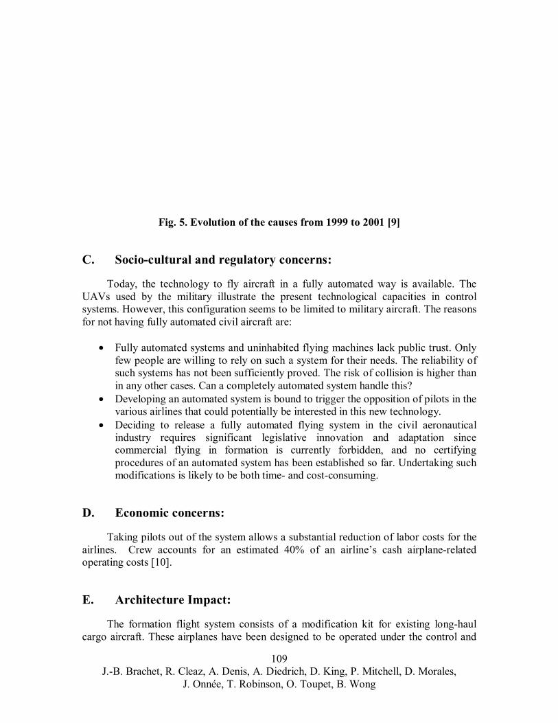
Fig. 5. Evolution of the causes from 1999 to 2001 [9]
C. Socio-cultural and regulatory concerns:
Today, the technology to fly aircraft in a fully automated way is available. The UAVs used by the military illustrate the present technological capacities in control systems. However, this configuration seems to be limited to military aircraft. The reasons for not having fully automated civil aircraft are:
• Fully automated systems and uninhabited flying machines lack public trust. Only few people are willing to rely on such a system for their needs. The reliability of such systems has not been sufficiently proved. The risk of collision is higher than in any other cases. Can a completely automated system handle this?
• Developing an automated system is bound to trigger the opposition of pilots in the various airlines that could potentially be interested in this new technology.
• Deciding to release a fully automated flying system in the civil aeronautical industry requires significant legislative innovation and adaptation since commercial flying in formation is currently forbidden, and no certifying procedures of an automated system has been established so far. Undertaking such modifications is likely to be both time- and cost-consuming.
D. Economic concerns:
Taking pilots out of the system allows a substantial reduction of labor costs for the airlines. Crew accounts for an estimated 40% of an airline’s cash airplane-related operating costs [10].
E. Architecture Impact:
The formation flight system consists of a modification kit for existing long-haul cargo aircraft. These airplanes have been designed to be operated under the control and
109 J.-B. Brachet, R. Cleaz, A. Denis, A. Diedrich, D. King, P. Mitchell, D. Morales,
J. Onnée, T. Robinson, O. Toupet, B. Wong

supervision of two pilots. The cost, both financial and technical, of removing these pilots from the airplane is not negligible. New software for operating the aircraft in configurations in which humans currently operate the aircraft would have a high cost of development and would have to be integrated with an architecture that was not originally designed to be operated under these circumstances.
If humans are taken out of the piloting loop and aircraft behave as UAVs, several questions are raised:
• How can the existing interfaces between operators and the UAVs in the case of the military be adapted to cargo aircraft?
• How well can the configuration and behavior of aircraft in the formation be reported to the person on the ground?
This latter question is already answering itself. The best way to understand a situation is to have a person present in that situation. A challenge with a fully-automated system is to accurately represent reality; therefore it must make its own decisions. The task of the controller on the ground would only be to command some modification in the general route followed by the formation and to check its global status. However, it appears highly complex to fly cargo airplanes in the same way pointer UAV’s are piloted, as the close proximity of the airplanes tends to add a large number of control parameters. Management of these parameters is likely to have a strong impact on the general safety of the convoy.
The system uses both pilots and automation in order to balance the competing objectives outlined above. Navigation and control operations are monitored by an automated control system. Pilots are responsible for operating their aircraft as in solo flights for all the phases in which the plane is not considered to be part of the formation. In other phases, the control is performed by the Formation Flight Manager, with the notable exception of emergency procedures, in which the pilot manually leaves the formation. The transition from solo flight to formation flight is determined by the new minimum horizontal separation requirement recommended in Appendix… A 1nm horizontal distance is suggested between ‘solo’ airplanes. Therefore a 2000ft-high and 2nm-wide cylinder around the formation would set the limit within which aircraft should be under control of the Formation Flight Manager. TCAS has the capability of providing pilots the distance to their close neighbors and can be used by the crew to switch the formation autopilot on.
F. Human Interface:
Pilots cannot be assigned the task of maintaining position in formation on a transcontinental or transoceanic flight. However, an interface is required between the control system and the pilots.
The goal is to implement an instrument that alleviates the pilots’ workload by providing them with information about the probability of a collision to help them decide
110 J.-B. Brachet, R. Cleaz, A. Denis, A. Diedrich, D. King, P. Mitchell, D. Morales,
J. Onnée, T. Robinson, O. Toupet, B. Wong
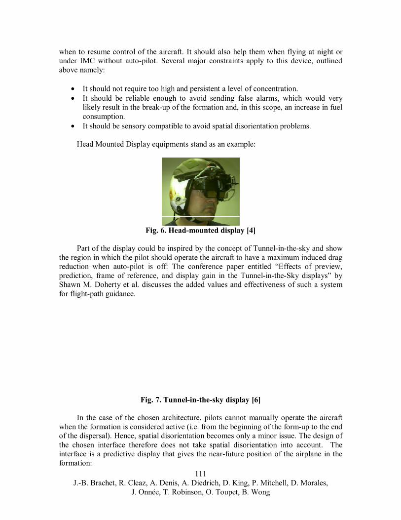
when to resume control of the aircraft. It should also help them when flying at night or under IMC without auto-pilot. Several major constraints apply to this device, outlined above namely:
• It should not require too high and persistent a level of concentration. • It should be reliable enough to avoid sending false alarms, which would very
likely result in the break-up of the formation and, in this scope, an increase in fuel consumption.
• It should be sensory compatible to avoid spatial disorientation problems.
Head Mounted Display equipments stand as an example:
Fig. 6. Head-mounted display [4]
Part of the display could be inspired by the concept of Tunnel-in-the-sky and show the region in which the pilot should operate the aircraft to have a maximum induced drag reduction when auto-pilot is off: The conference paper entitled “Effects of preview, prediction, frame of reference, and display gain in the Tunnel-in-the-Sky displays” by Shawn M. Doherty et al. discusses the added values and effectiveness of such a system for flight-path guidance.
Fig. 7. Tunnel-in-the-sky display [6]
In the case of the chosen architecture, pilots cannot manually operate the aircraft when the formation is considered active (i.e. from the beginning of the form-up to the end of the dispersal). Hence, spatial disorientation becomes only a minor issue. The design of the chosen interface therefore does not take spatial disorientation into account. The interface is a predictive display that gives the near-future position of the airplane in the formation:
111 J.-B. Brachet, R. Cleaz, A. Denis, A. Diedrich, D. King, P. Mitchell, D. Morales,
J. Onnée, T. Robinson, O. Toupet, B. Wong
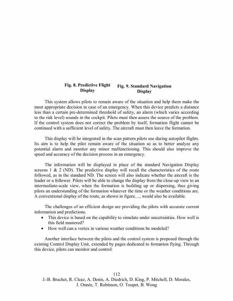
Fig. 8. Predictive Flight Fig. 9. Standard Navigation Display Display
This system allows pilots to remain aware of the situation and help them make the most appropriate decision in case of an emergency. When this device predicts a distance less than a certain pre-determined threshold of safety, an alarm (which varies according to the risk level) sounds in the cockpit. Pilots must then assess the source of the problem. If the control system does not correct the problem by itself, formation flight cannot be continued with a sufficient level of safety. The aircraft must then leave the formation.
This display will be integrated in the scan pattern pilots use during autopilot flights. Its aim is to help the pilot remain aware of the situation so as to better analyze any potential alarm and monitor any minor malfunctioning. This should also improve the speed and accuracy of the decision process in an emergency.
The information will be displayed in place of the standard Navigation Display screens 1 & 2 (ND). The predictive display will recall the characteristics of the route followed, as in the standard ND. The screen will also indicate whether the aircraft is the leader or a follower. Pilots will be able to change the display from the close-up view to an intermediate-scale view, when the formation is building up or dispersing, thus giving pilots an understanding of the formation whatever the time or the weather conditions are. A conventional display of the route, as shown in figure…, would also be available.
The challenges of an efficient design are providing the pilots with accurate current information and predictions.
• This device is based on the capability to simulate under uncertainties. How well is this field mastered?
• How well can a vortex in various weather conditions be modeled?
Another interface between the pilots and the control system is proposed through the existing Control Display Unit, extended by pages dedicated to formation flying. Through this device, pilots can monitor and control:
112 J.-B. Brachet, R. Cleaz, A. Denis, A. Diedrich, D. King, P. Mitchell, D. Morales,
J. Onnée, T. Robinson, O. Toupet, B. Wong
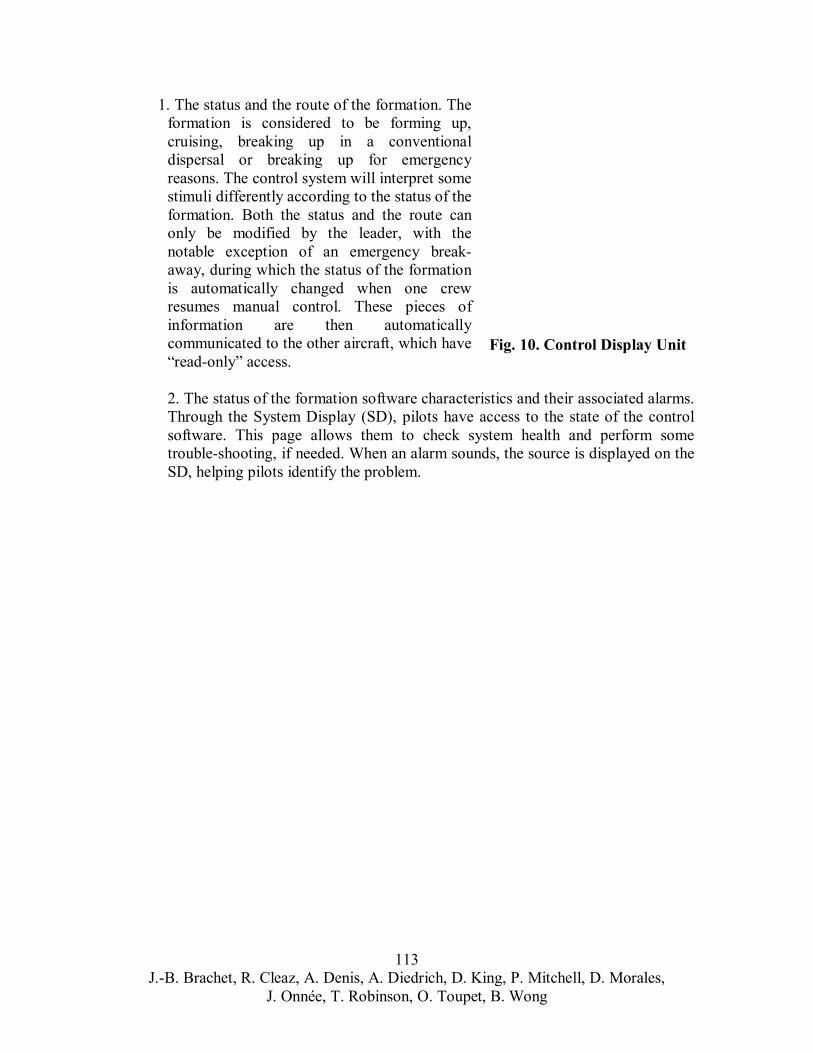
1. The status and the route of the formation. The formation is considered to be forming up, cruising, breaking up in a conventional dispersal or breaking up for emergency reasons. The control system will interpret some stimuli differently according to the status of the formation. Both the status and the route can only be modified by the leader, with the notable exception of an emergency break-away, during which the status of the formation is automatically changed when one crew resumes manual control. These pieces of information are then automatically communicated to the other aircraft, which have Fig. 10. Control Display Unit “read-only” access.
2. The status of the formation software characteristics and their associated alarms. Through the System Display (SD), pilots have access to the state of the control software. This page allows them to check system health and perform some trouble-shooting, if needed. When an alarm sounds, the source is displayed on the SD, helping pilots identify the problem.
113 J.-B. Brachet, R. Cleaz, A. Denis, A. Diedrich, D. King, P. Mitchell, D. Morales,
J. Onnée, T. Robinson, O. Toupet, B. Wong

Acknowledgement and references:
[1] Missy L Cummings, Boeing Associate Professor, Massachusetts Institute of Technology [2] F/A-18 Performance Benefits Measured During the Autonomous Formation Flight Project by J.Vachon, R.J.Ray, K.R.Walsh & K.Ennix, NASA, September 2003 [3] Induced Moment Effects of Formation Flight Using two F/A-18 Aircraft by J.L.Hansen & B.R.Cobleigh, NASA, August 2002 [4] Conflict between the Human Sensory System and Cockpit Design Standards by F.Patterson NAMRL [5] Visual, Cruise Formation Dynamics by S.Houck & J.D.Powell, Stanford University, 2000. [6] Effects of Preview, Prediction, Frame of Reference, and Display Gain in Tunnel-in-the-Sky Displays by S.Doherty of ERA University & C.D.Wickens of ULUC, 2001 [7] Training Transfer of a Formation Flight Trainer by G.B.Reid, Air Force Human Resources Laboratory, 1975. [8] http://membres.lycos.fr/belldandy/aeromedecine.html [9] http://www.math-info.unive-paris5.fr [10] Cost and Financial Analysis, K. Willcox lecture, 16.885, Massachusetts Institute of Technology, Sept. 16, 2003
114 J.-B. Brachet, R. Cleaz, A. Denis, A. Diedrich, D. King, P. Mitchell, D. Morales,
J. Onnée, T. Robinson, O. Toupet, B. Wong

115 J.-B. Brachet, R. Cleaz, A. Denis, A. Diedrich, D. King, P. Mitchell, D. Morales,
J. Onnée, T. Robinson, O. Toupet, B. Wong

XI. Multidisciplinary System Design Methods
116 J.-B. Brachet, R. Cleaz, A. Denis, A. Diedrich, D. King, P. Mitchell, D. Morales,
J. Onnée, T. Robinson, O. Toupet, B. Wong
A. Introduction
Some of the techniques in the field of multidisciplinary design optimization may be useful in the design of a formation flight transportation system.
Multidisciplinary design optimization is defined in a number of related ways. The following three definitions are from [1]:
• A methodology for the design of complex engineering systems and subsystems that coherently exploits the synergism of mutually interacting phenomena.
• Optimal design of complex engineering systems, which requires analysis that accounts for interactions amongst the disciplines.
• How to decide what to change, and to what extent to change it, when everything influences everything else.
The most important concepts are that it is multidisciplinary and that it normally involves mathematical optimization. A multidisciplinary problem is one comprised of more than one traditional disciplinary area described by a set of governing equations. For instance, a formation flight model using aerodynamic, economic, and control equations is multidisciplinary. The goals of using these tools are to gain design knowledge earlier and retain design freedom longer into development process and to control lifecycle costs by incorporating more disciplines and increasing the speed of the design process.
B. Elements of MDO
The most important elements of MDO are objectives, constraints, design variables, parameters, and simulation models.
a) Objectives The objectives are a vector of system responses or characteristics that are to be
maximized or minimized. These must be specific and measurable quantities. Often, a problem includes a set of conflicting objectives. These may be combined into a single objective through weighting or their interactions may be explored using multi-objective methods, such as the calculation of a Pareto front.
b) Constraints Constraints define the boundaries of the design space. Common constraints
include: 1. Physical laws, such as a constraint that lift must be at least equal to weight, or that
the Navier-Stokes equations must be satisfied in a computational fluid dynamics simulation
2. Finiteness of resources, such as an upper bound on the total cost of a system. 3. Technological limitations of the design variables, such as a minimum gauge for
the thickness of a wing skin. 4. Applicability of models, such as limits on the Reynolds number or Mach number
for a particular computational model to be valid. Constraints can be closed form or simulated functions of the design variables and
objectives.
117 J.-B. Brachet, R. Cleaz, A. Denis, A. Diedrich, D. King, P. Mitchell, D. Morales,
J. Onnée, T. Robinson, O. Toupet, B. Wong
c) Design variables Design variables are those values that the designer believes are under his control.
They must be specific and measurable values. Design variables can be continuous, such as the spacing between aircraft, discrete, such as the number of aircraft in a formation, boolean, such as whether an aircraft is piloted, or selection, such as the choice of communication systems to use in an aircraft. Most algorithms are best suited to one or another type of design variables; for instance, gradient-based methods work best on problems with continuous design variables while genetic algorithms are better suited to discrete or selection variables.
d) Parameters Parameters are variables that affect the objective and that the designer does not
believe are under his control. An example of a parameter for a formation flight system is the demand for air cargo. Parameters do not necessarily have to be known, but values are often assumed to perform the analysis. Robust design varies the parameters according to their probabilities and uses the expected value of the objectives as an objective function.
e) Models Finally, an MDO problem requires simulation models to link the design variables
and parameters to the objectives and constraints. Models are normally one of two types: physics models and empirical models. An example of a physics model is a Navier-Stokes analysis of the flow around an aircraft. This is built up from the fundamental assumptions of continuum mechanics as understood by aerodynamicists. An example of an empirical model is a regression analysis of the list prices of aircraft of a certain size used to predict the price of a similarly sized aircraft.
Many multidisciplinary models will use both types across the disciplines and combine them to calculate the objectives and constraints.
The challenge in finding models for MDO is balancing the tradeoff between computational time and model fidelity. Since MDO algorithms call the model simulation thousands of times, depending on the number of design variables, the computational time for a single analysis has a large effect on the total cost of the optimization. However, fast models often have low fidelity, and optimization of a low-fidelity model can often not be trusted to find an optimum close to the real-world best design. In fact, many optimizers exploit simplifications of the model and will choose unrealistic designs in low-fidelity models.
C. Mathematical formulation
In multidisciplinary optimization, the design problem is expressed as a mathematical problem. In particular, it is expressed as the minimization of some vector (called J below) comprising quantitative measures of system behavior. The problem can also be constrained with equality and inequality constraints and by bounds on the design problems. In mathematical language, every optimization problem can be expressed in the following standard form:
118 J.-B. Brachet, R. Cleaz, A. Denis, A. Diedrich, D. King, P. Mitchell, D. Morales,
J. Onnée, T. Robinson, O. Toupet, B. Wong
Minimize by varying x: p x J )( , Subject to:
p x g ) ≤ 0( , p x h ) = 0( ,
where J is a vector of objectives, x is a vector of design variables, p is a vector of parameters, and g and h are vectors of inequality and equality constraints.
MDO algorithms mathematically trace a path in the design space from some initial design towards improved designs. Their advantage is that they operate on a large number of variables and functions simultaneously in a way that is difficult for humans. One aspect of these algorithms that can be considered either an advantage or a disadvantage is that this path is not biased by intuition or experience.
The following is the standard process involved in optimizing a multidisciplinary design problem:
1. Define the system requirements 2. Choose the design vector, the objectives, and the constraints 3. Decompose the system into simpler modules 4. Model the physics (or economics etc) of the problem at the module level 5. Integrate the model into a system simulation 6. Benchmark the model by comparing it to known solutions 7. Explore the design space, often using methods drawn from design of experiments
theory 8. Optimize the problem to minimize the objective, subject to the constraints. 9. Perform a sensitivity analysis in order to evaluate the formulation of the problem
and understand the design space in the neighborhood of the solution found by the optimizer.
D. History
Over the history of aircraft design, the design requirements have grown and changed. At the beginning of the century, the only requirement was feasibility, that is, an airplane that would fly. Later development emphasized performance. In the last two decades, new metrics have been devised to evaluate aircraft, such as lifecycle cost, and the “ilities”: reliability, maintainability, etc.
Computer aided design and analysis has made it possible for much of the mathematical and bookkeeping work to be done by computers. In addition, procurement policy has changed for airlines military, putting more emphasis on lifecycle cost and the “ilities” over performance.
Since 1990, MDO has evolved significantly. It has extended to a number of industries including automobiles, spacecraft, and power systems. It has moved to global, decentralized design teams and from super-computers to groups of high-performance personal computers. Disciplinary software such as Nastran for structures and Fluent for fluid dynamics are now very mature and reliable. The Internet and local area networks
119 J.-B. Brachet, R. Cleaz, A. Denis, A. Diedrich, D. King, P. Mitchell, D. Morales,
J. Onnée, T. Robinson, O. Toupet, B. Wong

allow for easy information transfer. Currently, there are many research groups inventing and improving optimization algorithms, and there exists commercial off-the-shelf MDO software.
E. Advantages of MDO
Single disciplines often have conflicting goals. When not considering the fully coupled problem, disciplinary specialists tend to generate side effects in other disciplines. For example, it is traditional in aircraft design for aerodynamicists to first design the outer old line of the aircraft, and the structural experts are required to fit their design within that space. MDO incorporates and explores tradeoffs in a disciplined way and therefore allows for a “better” design, as measured by the objectives. It allows the designer to include concurrent engineering disciplines such as manufacturing, supportability, and cost. Used properly, it can result in a reduction of the design time. It handles a wide variety of design variables and constraints. The designs found are not biased by intuition or experience, which can be an advantage when it finds unexplored areas of the design space, but can be a disadvantage due its lack of “common sense.”
F. Disadvantages of MDO
However, MDO requires mathematical models of objectives, constraints, and their inter-relationships early in the design process. It is not a push-button system and does not replace good engineering judgment. Unlike a human designer, it will work only within the limits set by the problem formulation and is unlikely to find an innovative design. When it does find an “optimum” design according to the given objectives, that doesn’t always mean it has found the best design in a real-world sense. Computational time grows rapidly with number of design variables and the solution is often highly dependent on numerical issues such as scaling and the non-linearity of the problem. The design space is limited to the range of applicability of the analysis models and the optimizer will take advantage of analysis errors or modeling limitations to provide “mathematical” design improvements that do not translate to an improvement in the real design.
G. Available Techniques
MDO includes a number of techniques to explore the design space and find improved designs.
a) Design-Space exploration Design-space exploration is the process of evaluating a number of designs in order
to gain further understanding of the design space and the effects of the variables on the objectives. It uses statistical techniques to provide a systematic way to sample the design space. Many methods exist, including full factorial, orthogonal arrays, one at a time exploration, Latin hypercubes, and parameter study. All of them attempt to quantify the effects on the objectives of changing the design variables to a number of discrete values. It is useful when tackling a new problem when little is known about the design space. It can help the designer identify the most important design drivers among the design
120 J.-B. Brachet, R. Cleaz, A. Denis, A. Diedrich, D. King, P. Mitchell, D. Morales,
J. Onnée, T. Robinson, O. Toupet, B. Wong
variables, select appropriate ranges for the design variables, and estimate achievable values for the objective functions. A disadvantage is that it doesn’t immediately suggest a design. It is often useful in conjunction with other MDO techniques, for instance, to choose an initial guess for a gradient-based method.
b) Gradient-Based Optimization Methods Gradient-based optimization techniques are methods that use gradient information
to find local minimum of the objectives from a given starting point. For example, steepest descent, conjugate gradient, and sequential quadratic programming are gradient-based methods. They are normally iterative, that is, they perform the same steps many times, moving from one location in the design space to another. They require a gradient calculation, which can be performed using analytic differentiation, automatic differentiation, adjoint methods, or finite differences. These methods tend to be fast relative to many other methods, and it can be numerically proven that an appropriately conditioned problem will converge to a local optimum. However, there is never a guarantee that it has found the global optimum. There may be multiple solutions. It is common to begin these methods at a number of initial guesses in order to find a number of local minima to compare. These methods are often very sensitive to numerical ill conditioning.
c) Other Optimization Methods Other types of optimization methods include genetic algorithms, simulated
annealing, and particle swarm optimization. They are used in order to escape the local optima found by gradient-based methods. Many of these have become very popular in the last 10 years. Population-based methods such as genetic algorithms and particle swarm optimization are often have good design space coverage and treatment of discrete decisions, but are very computationally expensive. This class of methods is also sensitive to tuning parameters that need to be adjusted by the designer, often through trial and error.
d) Local Trade Studies and Parametric Studies, and Sensitivity Analysis Other techniques that can be used from MDO are local trade studies, parametric
studies, and sensitivity analysis. These can help the designer explore the tradeoffs between competing objectives, or evaluate the changes in the objectives as design variables or parameters are varied. It can help a design team resolve competing disciplinary needs. It does not suggest a design, but rather, serves as an informational source for the designer. It can also show which constraints are active, and examine the effects on the objectives of changing the constraints. This can help the designer re-formulate the problem and evaluate the importance of the constraints.
H. MDO Applied to Formation Flight
For a formation flight project, the methods of MDO can help in a number of ways. It can contribute to an understanding of the tradeoff of the disciplines, such as between the cost of control precision and the fuel benefits from precise control. It can analyze the overall system when a number of parameters vary, such as the magnitude of the
121 J.-B. Brachet, R. Cleaz, A. Denis, A. Diedrich, D. King, P. Mitchell, D. Morales,
J. Onnée, T. Robinson, O. Toupet, B. Wong
aerodynamic benefits. When models are available, optimization methods will be able to find the optimum design. It can also be used to perform sensitivity analysis to evaluate the formulation of the problem
Many of these methods require much more information about the problem than is currently available. The vortex mapping and market analysis in the program plan will be most helpful in enabling MDO.
The design of a formation flight system is a significant challenge for MDO. This problem has a large number of possible design variables, objectives, and constraints. Many of the objectives and constraints are difficult to quantify and model. The models that exist, such as those for the position and strength of vortices, are immature. The lack of benchmarks makes it difficult to validate the models. The design variables are both mixed and continuous, which presents numerical obstacles for a number of optimization techniques. This problem also has large amounts of interdisciplinary coupling, making it more complex and less amenable to decomposition.
I. Conclusion
The formation flight models available today do not have adequate fidelity for a full use of MDO methods. However, the complex, new, and interdisciplinary nature of the design of a formation flight system make it a good candidate for MDO in the later design stages.
122 J.-B. Brachet, R. Cleaz, A. Denis, A. Diedrich, D. King, P. Mitchell, D. Morales,
J. Onnée, T. Robinson, O. Toupet, B. Wong

References
[1] AIAA Multidisciplinary Design Optimization Technical Committee, What is MDO, available http//endo.sandia.gov/AIAA_MDOTC/main.html, cited May 13, 2003
[2] K. Willcox and O. de Weck, Multidisciplinary System Design Optimization Introduction, Lecture, 16.888 class, Massachusetts Institute of Technology, February 4th, 2004
123 J.-B. Brachet, R. Cleaz, A. Denis, A. Diedrich, D. King, P. Mitchell, D. Morales,
J. Onnée, T. Robinson, O. Toupet, B. Wong

XII. Key Trade-Off’s
124 J.-B. Brachet, R. Cleaz, A. Denis, A. Diedrich, D. King, P. Mitchell, D. Morales,
J. Onnée, T. Robinson, O. Toupet, B. Wong
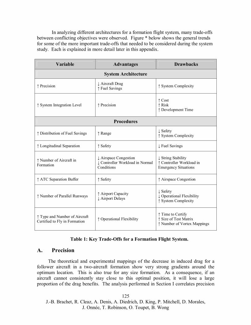
In analyzing different architectures for a formation flight system, many trade-offs between conflicting objectives were observed. Figure * below shows the general trends for some of the more important trade-offs that needed to be considered during the system study. Each is explained in more detail later in this appendix.
Variable
Precision
System Integration Level
Distribution of Fuel Savings
Longitudinal Separation
Number of Aircraft in Formation
ATC Separation Buffer
Number of Parallel Runways
Type and Number of Aircraft Certified to Fly in Formation
Advantages Drawbacks
System Architecture
Aircraft Drag Fuel Savings System Complexity
Precision Cost Risk Development Time
Procedures
Range Safety System Complexity
Safety Fuel Savings
Airspace Congestion Controller Workload in Normal
Conditions
String Stability Controller Workload in
Emergency Situations
Safety Airspace Congestion
Airport Capacity Airport Delays
Safety Operational Flexibility System Complexity
Operational Flexibility Time to Certify Size of Test Matrix Number of Vortex Mappings
Table 1: Key Trade-Offs for a Formation Flight System.
A. Precision
The theoretical and experimental mappings of the decrease in induced drag for a follower aircraft in a two-aircraft formation show very strong gradients around the optimum location. This is also true for any size formation. As a consequence, if an aircraft cannot consistently stay close to this optimal position, it will lose a large proportion of the drag benefits. The analysis performed in Section I correlates precision
125 J.-B. Brachet, R. Cleaz, A. Denis, A. Diedrich, D. King, P. Mitchell, D. Morales,
J. Onnée, T. Robinson, O. Toupet, B. Wong
of station-keeping with fuel savings. The following results were obtained for a formation of two aircraft:
10% fuel savings for perfect station-keeping 8% fuel savings for 0.1 wingspan precision 6% fuel savings for 0.2 wingspan precision
Nearly half of the expected benefits are lost when the overall distance-keeping precision degrades to 0.2 of a wingspan. The problem is that achieving this precision requires new technologies in instrumentation and inherently more complex control algorithms. Care must be taken that the benefit of greater precision is not outweighed by the possible additional fuel used to achieve it. In general, the greater the precision desired, the more changes that will need to be made to existing aircraft. This means an increase in development and certification costs as well as program risk. This is detailed a bit more below.
B. System Integration Level
System integration level is a measure of how much new technologies introduced by the formation flight system change existing ones already on the aircraft. This is closely related to the number of new technologies, but also takes into account the difficulty needed to integrate these upgrades into the system.
The best example of the system integration level trade-off is in the contrast between possible architectures for the formation flight control system. The options are to use the existing autopilot or an entirely new autopilot (as part of the formation manager). Both are upgrades to the existing system, but engineering a box to create custom inputs to the existing autopilot is a much easier task than designing an autopilot from scratch. It will be less risky to certify due to a smaller incremental change from existing systems, and its simpler nature will require less development time. Both of these factors directly impact overall cost of the system, both at the developer and customer levels. The benefit of creating an entirely new autopilot is that the formation system will have better control of the aircraft. Being one less degree of separation from the flight computers will result in better control performance, thus improving precision of the station-keeping. The real question then becomes if this additional precision is required or justified based on its incremental improvement.
C. Shape of the Formation
a) Distribution of the Benefits As explained in Section I, fuel savings can be equally distributed between aircraft
by rotating in an echelon formation. This is the easiest configuration to rotate in that optimizes entire formation benefits. Rotation is the only way to get range benefits from formation flight, otherwise only fuel benefits are possible. Moreover, the more often rotation occurs, the more elliptical the lift distribution becomes, resulting in greater benefits for the whole formation. However, the complexity of the system is also increased by rotation, since it involves reconfiguration of the formation in a periodic fashion. This
126 J.-B. Brachet, R. Cleaz, A. Denis, A. Diedrich, D. King, P. Mitchell, D. Morales,
J. Onnée, T. Robinson, O. Toupet, B. Wong
means that the autopilot will likely have to be adapted in order to control the rotations, and that the leader aircraft will not always be at the same position within the formation. Some fuel might also be wasted during the rotation due to aircraft accelerating during reconfigurations. Finally, collision risk is increased as the front aircraft moves to the back during a rotation.
b) Longitudinal Separation The longitudinal separation between aircraft in the formation is the result of a trade-
off between two parameters: safety and fuel savings. The further away from the lead aircraft, the weaker the wingtip vortex is and the harder it is to actually locate. Common sense dictates that the larger the longitudinal separation, the less collision risk there is, and thus the higher the safety. Experimental results suggest that the strongest benefits are attained for a longitudinal distance of 3-7 wingspans, so a compromise between safety and performance can be achieved by specifying a following distance of 7 wingspans.
c) Number of Aircraft in the Formation Many parameters influence the choice of the number of aircraft in a given
formation. The greater the number of aircraft in a formation, the higher the possible overall realizable benefits will be. This is because the effect of the leader not getting any benefits is more spread out in larger formations. However, with more aircraft in formation it is in general harder to maintain string stability. Greater coordination is required and there is more opportunity for errors to propagate towards the back of the formation, though with the proposed centralized leader-follower control scheme this is not an issue. It becomes more of an issue when each aircraft finds its relative position only with respect to adjacent airplanes, as may be the case in some potential formation flight systems.
Operations also have an influence on this trade-off. Having more aircraft in a formation decreases congestion of airspace and the workload on ATC controllers while the aircraft are flying in formation. This is because each formation is considered a single entity in terms of airspace and point of contact for ATC. On the other hand, in emergency situations the formation will break up and ATC will be forced to direct individual aircraft again. With higher numbers in the formation, the workload upon ATC controllers is increased and may exceed an individual’s capacity to safely manage the situation.
D. ATC separation buffer
From an operations standpoint, the main advantage of flying in formation is to decrease airspace congestion. Increasing the separation buffer means increasing the volume attributed to a formation, and therefore decreasing the precedent benefit. At the same time, increasing the separation buffer also means decreasing the risk of collisions, which is could be especially catastrophic with so many aircraft in close proximity.
127 J.-B. Brachet, R. Cleaz, A. Denis, A. Diedrich, D. King, P. Mitchell, D. Morales,
J. Onnée, T. Robinson, O. Toupet, B. Wong
E. Number of Parallel Runways
A significant difficulty of flying in formation is the join-up procedure. If the aircraft all take-off from different runways and meet at a given rendezvous point, there is a high probability that there will be delays on at least some of the runways. One or several aircraft will have to loiter, wasting fuel and cutting into the overall formation benefits. A way to decrease this waiting time is to have the aircraft take off together from parallel runways. This solution will also permit airports to use parallel runways at the same time, which is normally not possible for safety reasons. This leads to an increase in the airport capacity and a decrease in take-off delays by increasing take-off rates. Landing on parallel runways could also happen, giving the same benefits to the destination airport. However, the other side can be examined--requiring the simultaneous use of multiple runways could decrease operational flexibility, and time periods when multiple runways are available might be rare.
Another major disadvantage of this procedure is that there are increased collision risks by having multiple aircraft in such close proximity during the critical take-off and landing phases of flight. Moreover, the formation autopilot will likely be required to have a special mode developed in order to be able to manage these take-offs and approaches. They cannot be safely done by human pilots.
F. Type and Number of Aircraft Certified to Fly in Formation
The certification process must be done for each individual aircraft type and arguably also for each size of formation to be flown. As the numbers and aircraft types certified to fly in formation goes up, a wider range of missions using formation capability will become possible.
However, as with any certification process, this takes time. Each certification will require numerous test flights, with increasing volume as the number of possible combinations goes up. For example, say that the Boeing 747 is certified to fly in formation. It would first be certified to fly only in formations with other 747s. As a later process, additional test flights and certification would take place to ensure the safety of flying 747s and Airbus A380s (or any other type of long haul cargo aircraft) flying in the same formation. If flying 747s with Boeing 777s in formation was desired, then the same process would have to be followed. To be able to use all three of these types of aircraft in formation interchangeably, certification to fly A380s with 777s as well as flying all three types at once would have to be pursued. A similar multiplying effect applies to the number of aircraft certified to fly in formation. All of these different permutations are collectively referred to as the test matrix, and from the example it can be seen how quickly it grows as the number and type of aircraft certified to fly in formation goes up.
For each aircraft type, mapping the drag reduction as a function of relative position must be done so that the station-keeping algorithm can be used to maximize the benefits of formation flight. It is a linear function of the number of aircraft certified to fly in formation.
128 J.-B. Brachet, R. Cleaz, A. Denis, A. Diedrich, D. King, P. Mitchell, D. Morales,
J. Onnée, T. Robinson, O. Toupet, B. Wong

129 J.-B. Brachet, R. Cleaz, A. Denis, A. Diedrich, D. King, P. Mitchell, D. Morales,
J. Onnée, T. Robinson, O. Toupet, B. Wong

XIII. Architecture Selection
130 J.-B. Brachet, R. Cleaz, A. Denis, A. Diedrich, D. King, P. Mitchell, D. Morales,
J. Onnée, T. Robinson, O. Toupet, B. Wong
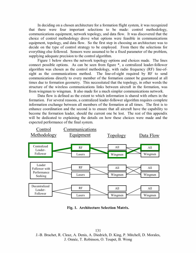
In deciding on a chosen architecture for a formation flight system, it was recognized that there were four important selections to be made: control methodology, communications equipment, network topology, and data flow. It was discovered that the choice of control methodology drove what options were feasible in communications equipment, topology, and data flow. So the first step in choosing an architecture was to decide on the type of control strategy to be employed. From there the selections for everything else followed. Sensors were assumed to be a fixed parameter of the problem, supplying adequate precision to the control algorithm.
Figure 1 below shows the network topology options and choices made. The lines connect possible options. As can be seen from figure *, a centralized leader-follower algorithm was chosen as the control methodology, with radio frequency (RF) line-of-sight as the communications method. The line-of-sight required by RF to send communications directly to every member of the formation cannot be guaranteed at all times due to formation geometry. This necessitated that the topology, in other words the structure of the wireless communications links between aircraft in the formation, was from wingman to wingman. It also made for a much simpler communications network.
Data flow is defined as the extent to which information is shared with others in the formation. For several reasons, a centralized leader-follower algorithm requires complete information exchange between all members of the formation at all times. The first is to enhance coordination and the second is to ensure that all aircraft have the capability to become the formation leader, should the current one be lost. The rest of this appendix will be dedicated to explaining the details on how these choices were made and the expected performance of the final system.
Control Communications Methodology Equipment Topology Data Flow
RF
RF
RF
Centralized Leader-
Follower
Leader Follower with Performance
Seeking
Decentralized Leader-
Follower
Lasers
Lasers
Lasers
All
Wingmen
All
Wingmen
All
Wingmen
All
Wingmen
All
Wingmen
All
Wingmen
Fig. 1. Architecture Selection Matrix.
131 J.-B. Brachet, R. Cleaz, A. Denis, A. Diedrich, D. King, P. Mitchell, D. Morales,
J. Onnée, T. Robinson, O. Toupet, B. Wong
A. Control Methodology
a) Options
The various options, as detailed in Appendix *, are described here again with regards to their specific pros and cons in application to formation flight of air cargo transport aircraft. It should be noted that in some cases, the various methods can be combined into a hybrid type of algorithm. They fall into two main categories:
Model-based Methods
Model-based methods in general tend to be traditional and proven in applications other than aircraft formation flight, such as in UAVs, vehicle platoons, or satellite clusters. They involve smaller development effort and risks to implement than non model-based methods.
(a) Trajectory Tracking
Pros • The simplest method to implement, as it has been used extensively in related
applications to formation flight and is the least complex in operation. • Easy to predict resulting flight behavior, and thus to certify. • Little or no communication between aircraft is required for some
configurations.
Cons • Operationally inflexible. • Level of performance achievable with lack of constant reference to other
airplanes in the formation is probably unacceptable.
(b) Leader-Follower Station-Keeping
Pros • This is the only method known to perform within the range of required
accuracy in formation flight tests (outside of the wingtip vortex) [1]. • Has also been extensively simulated with promising results in numerous
articles [2,3,4,5,6,7]. • A flexible method with there are many different implementations:
o Leader, front and hybrid modes, formation geometry center concept. o Centralized or decentralized.
132 J.-B. Brachet, R. Cleaz, A. Denis, A. Diedrich, D. King, P. Mitchell, D. Morales,
J. Onnée, T. Robinson, O. Toupet, B. Wong

Cons • The theoretically optimal relative position, or even one determined by vortex-
mapping, may not be the true optimal position for maximum drag reduction benefits.
• The amount of flight-testing to completely map the vortex for combinations of flight conditions, numbers of aircraft, and types of aircraft would be substantial.
Non Model-based Methods
Non model-based methods are generally experimental and are in a less mature stage of development than most model-based methods. Some, such as neural networks, are already in use in loosely related applications such as process control, while others, such as vortex shaping, are only paper ideas. They will require a larger development effort and have higher risks to implement than model-based methods, but they can also potentially achieve greater performance benefits.
(a) Performance Seeking
Pros • If working correctly, this algorithm will find the minimum drag location based
on actual flight data, and thus is capable of optimizing in real-time. • While application to aircraft formation flight is relatively new, the theory
behind performance seeking originates from the 1960s and has been used successfully in many other applications.
Cons • Difficult to achieve good performance when tracking large reference
distances, as the algorithm can more easily be side-tracked by local, transient drag minimums. This is a problem to a lesser extent when close to the true vortex location, but it remains a large issue.
• Current implementations of this algorithm require undesirable oscillation of control surfaces even under stable conditions.
• Very technical and complex in operation, will require a significant development effort to work out technical issues and train pilots on its sometimes non-intuitive behavior.
(b) Neural Networks
Pros • Does not require the use of relative position measurements.
Cons • Requires a comprehensive training set, probably similar to a vortex-mapping
program, but bigger.
133 J.-B. Brachet, R. Cleaz, A. Denis, A. Diedrich, D. King, P. Mitchell, D. Morales,
J. Onnée, T. Robinson, O. Toupet, B. Wong
• Can achieve good performance in non-aviation applications, but will be very tough to certify due to unpredictability when a condition outside of the training set is encountered.
(c) Vortex Shaping
Pros • Moving the vortex to where the trail aircraft is instead of the other way around
may be more fuel efficient. • May have applications outside of formation flight.
Cons • Requires extensive wing modifications (plus related development cost) to
existing aircraft, which goes against a general principal of the overall system goal to try and modify aircraft by the minimum amount possible.
• The aerodynamic theory is not yet well developed enough to predict the effects of changing wing geometry on vortex position to the level of accuracy required.
b) Algorithm Selection
The most promising control methods all fall under the general category of leader-follower station-keeping. The reason is that all the other methods have obvious problems including large uncertainty and risks associated with unproven technologies (all non model-based methods), certification issues (neural networks), extensive modifications to existing airplanes (vortex shaping), and unsatisfactory performance (trajectory tracking).
Centralized and de-centralized leader-follower were the two methods selected to be examined in greater detail, based upon their practicality and common usage in UAV systems today.
Performance seeking control, although requiring significant development, was also selected for further investigation due to its prospective performance benefits and synergies with leader-follower methods. Through concurrent development with the preferred leader-follower methods, it has two potential roles in a development plan. One is for risk mitigation as a viable control alternative, should leader-follower methods be unsatisfactory, and the other is as a performance upgrade upon an already functional, working system.
Centralized Leader-Follower
In this control methodology, there is a single commander aircraft within the formation that controls all the other aircraft. In other words, this leader aircraft issues all commands to the follower aircraft. These commands are designed to balance (at times) several competing goals in the appropriate manner. One goal is to optimize and maintain the overall formation shape, with planes offset by required relative distance to maximize drag
134 J.-B. Brachet, R. Cleaz, A. Denis, A. Diedrich, D. King, P. Mitchell, D. Morales,
J. Onnée, T. Robinson, O. Toupet, B. Wong
savings (feed-back). The other is to anticipate planned future maneuvers, and to compensate for them in advance (feed-forward). This relieves any string stability concerns. To reiterate, all that the follower aircraft do is receive high-level target relative state commands from the leader, and based on these, compute the low-level control inputs required to execute them.
Advantages • Decisions are made from a higher, system level, resulting in enhanced
coordination and a greater overall performance level. • Lower algorithm complexity (directly impacting cost). • Preferred for simple missions where performance is a priority.
Disadvantages • High volume of required communications. • Slower reaction times to unexpected changes.
De-Centralized Leader-Follower
This method follows the opposite philosophy of the previous one. De-centralization means that each aircraft in the formation tries to maintain relative position with the aircraft in front of it independently of anyone else. However, in order to maintain string stability, feed-forward is again employed in a slightly different manner. Each airplane receives information from aircraft ahead in the formation and the leader (which may be behind) as to intent and makes appropriate compensatory maneuvers at the appropriate times. Although this strategy was not chosen for the system design, it requires the same equipment as centralized. The difference between de-centralized and centralized would only be a software change.
Advantages • Less information must be exchanged. • Robust, flexible. • Formation reconfiguration and leader “hand-off” will be easier. • Preferred for complex missions, particularly where the number of airplanes in the
formation is expected to change.
Disadvantages • Distributed decision-making can result in less than efficient coordination through
conflicting decisions not benefiting the formation as a whole, or in the case of reconfiguration, changing mission goals, etc.
Performance Seeking
This methodology may be used by itself, or be combined with either of the two methods above in several ways. One way to integrate the two would be to use the leader-follower algorithm to hold an arbitrary tight relative position while performance seeking
135 J.-B. Brachet, R. Cleaz, A. Denis, A. Diedrich, D. King, P. Mitchell, D. Morales,
J. Onnée, T. Robinson, O. Toupet, B. Wong
directs where to hold that position (which will change over time). Another method would be to allow the pilot, or even automation, to decide which algorithm would perform better in a given situation, and to switch between the two. As mentioned in an earlier section, performance-seeking control tends to work better when already close to target, so it could be used selectively. Performance seeking could be done on an individual aircraft basis, or again be centralized. Adding in this option should be justified based on how much extra performance could be achieved with it, weighed against the extra complexity it adds.
Advantages • The entire system concept does not depend on this method working perfectly right
away; it is only a risk mitigation strategy in the beginning. • Potential for superior performance in conjunction with leader-follower methods or
by itself.
Disadvantages • Risky, as performance benefits in actual formation flight are relatively unknown. • High development costs.
c) Conclusions
The long haul air cargo market has simple, well-defined missions and obtaining maximum performance with the lowest ticketed price is a primary goal of the system. All of these needs point clearly to centralized leader-follower as the preferred control algorithm for a formation flight architecture. Performance seeking is a method which has good potential, but requires more development time, and as a result, has a higher associated risk. However, pursued concurrently as a back-up and enhancement to primary methods its development can be justified.
d) Expected Performance
Autonomous formation flight in the wingtip vortex has never been done, so it is difficult to estimate how well a particular control algorithm will do. However, with a centralized leader-follower control architecture it is reasonable to expect that precision within 0.1 of a wingspan of the required relative position may be achieved, given the appropriate sensor and communications information. If not, then as discussed above, performance seeking control may be pursued as an alternative and/or refinement.
Several research papers back-up this claim. Foremost among them is the NASA Autonomous Formation Flight (AFF) program, which in numerous flight tests of two F-18s using a decentralized leader-follower algorithm achieved an out of vortex lateral and vertical accuracy of +/- 9 feet in level flight, 100% of the time [1]. This corresponds to a maximum of 0.2 wingspan error, twice the target accuracy, but the algorithm used was a
136 J.-B. Brachet, R. Cleaz, A. Denis, A. Diedrich, D. King, P. Mitchell, D. Morales,
J. Onnée, T. Robinson, O. Toupet, B. Wong
basic one used only to demonstrate feasibility and not performance. It was not optimized or tweaked in any way.
Similarly, Proud, Pachter and D’Azzo ran simulations with two F-16s using a decentralized leader-follower algorithm [6]. They met the 0.1 wingspan performance requirement for level flight and maneuvering flight for instantaneous lead heading changes of +/- 20 degrees, lead velocity changes of +/- 50ft/s and lead altitude changes of +/- 400ft. In both these studies, de-centralized leader-follower algorithms were used, but for a two aircraft formation, centralized leader-follower would have similar results. The difference between the two methods becomes more apparent as the number of aircraft in the formation increases, due to how communications and coordination scale.
Many other simulations have also been run using leader-follower strategies that present less detailed results on general control performance, but they also give general indications that 0.1 wingspan accuracy is possible [4,7].
Lastly, subject matter experts John Deyst and Jon How at the Massachusetts Institute of Technology (MIT) are optimistic the chosen control methodology can achieve the desired accuracy based on their collective experience with UAVs.
B. Communications Equipment
The main choices for the means of communication are radio frequency (RF) and laser, and both require a clear line of sight to operate. In other applications, both methods have demonstrated the required data rate of 1-100 Hz and transmission distance to cover the formation; however radio waves are omni-directional, and thus do not need to be aimed as lasers do. Satellite-based communications, where all communications are relayed through a satellite, were also considered. Satellite communications were eliminated early on because of time-lag. Below are advantages and disadvantages for RF communications, laser communications, and satellite communications.
Radio Frequency Communications
Advantages • Used for many other common applications. • Transmitters and receivers are commercially available. • Lower cost. • Works through clouds and other weather. • Omni-directional (does not need to be specifically aimed at target receiver). • Capable of 1:N communications.
Disadvantages • May have conflicts with other equipment or frequencies both onboard aircraft and
external to the formation flight system. • Line-of-sight required for transmission including clear elliptical-shaped Fresnel
clearance zone. • Additional antennae may need to be installed on the exterior of the aircraft,
producing additional drag (including when not in formation), modification costs, and certification costs.
137 J.-B. Brachet, R. Cleaz, A. Denis, A. Diedrich, D. King, P. Mitchell, D. Morales,
J. Onnée, T. Robinson, O. Toupet, B. Wong
Laser Communications
Advantages • Low observability. • Unlikely to conflict with existing equipment. • Less physical clearance needed for transmission (only visual line of sight needed
and not Fresnel zone). • A new transmitter/receiver would be needed, but it can be inset and covered by an
optically transparent panel to avoid extra drag.
Disadvantages • Line of sight required for transmission. • Higher complexity. • Higher cost to implement. • Has not been used as extensively as RF communications. • Needs to be aimed at receiver i.e. unidirectional and is very sensitive to errors in
direction. • Beam-scatter in clouds and other unfavorable weather conditions.
Satellite Communications
Advantages • Line of sight not an issue
Disadvantages • Lower reliability • Long lag-time (~1.5 sec) in transmission makes satellites unfeasible.
Radio frequency communications are lower risk and lower cost. RF was chosen as the currently preferred method for inter-formation communications, while leaving open the possibility of using laser communications in the future as the technology matures.
C. Topology
Although the choices of network topology are infinite for a wireless network due to the lack of physical connections, the main choice for the formation flight system centered around two topologies. Both of them preserve symmetry given the limitations set by the formation shape and the commonality/safety requirement, which meant that any aircraft could be called upon to act as the leader and command-issuing nerve center of the formation. The first possible topology had all aircraft receiving information directly from all other aircraft. The second had aircraft only receiving information relayed through adjacent aircraft in the formation. Below are the advantages and disadvantages of the two topologies.
138 J.-B. Brachet, R. Cleaz, A. Denis, A. Diedrich, D. King, P. Mitchell, D. Morales,
J. Onnée, T. Robinson, O. Toupet, B. Wong

Information Directly Received From Other Aircraft
Advantages • More robust because of duplicate information paths. • If using RF, less messages need to be broadcast by taking advantage of 1:N
communications capability. • Symmetry allows easy rotation of formation leader.
Disadvantages • More power needed to transmit over long distances between non-adjacent aircraft. • If using lasers, frequent re-aiming necessary to hit different targets, or else
multiple lasers needed. • Clear path not necessarily available between non-adjacent aircraft.
Information Relayed Through Adjacent Aircraft
Advantages • Less power needed to transmit only to wingman. • If using lasers, frequent re-aiming not necessary. • Information can be consolidated. • Optimizes communications channels with shortest path network.
Disadvantages • If an aircraft in the middle of the formation loses communications, the network is
broken and must re-form. • During rotation of the formation, the former leader must break communications
with the formation while changing position to back of formation.
Although there were more or less equivalent advantages and disadvantages for each topology, a relay or “wingman” topology was chosen since the combination of an echelon formation with line-of-sight communications only allowed that topology to work. In other words, aircraft in between could block communications between non-adjacent aircraft in the formation.
D. Data Flow
Based on the decisions made for control methodology, communications equipment and network topology, a data flow system where all aircraft have information about all other aircraft in the formation follows. This allows the leader to send commands to all other aircraft in order to avoid string-stability problems, while maintaining symmetry in the system for ease of formation rotation. In addition, if partial or full communications are lost, having information about all other aircraft just prior to the loss allows the formation to safely break-up. This data flow is explained in more detail in the communications section of the appendices.
139 J.-B. Brachet, R. Cleaz, A. Denis, A. Diedrich, D. King, P. Mitchell, D. Morales,
J. Onnée, T. Robinson, O. Toupet, B. Wong
References
[1] Hanson, C.E., Ryan, J., Allen, M.J., and Jacobson, S.R., “An Overview of Flight Test Results for a Formation Flight Autopilot,” AIAA Paper 2002-4755, Aug. 2002.
[2] Hummel, D., “The Use of Aircraft Wakes to Achieve Power Reduction in Formation Flight,” Proceedings of the Fluid Dynamics Panel Symposium,AGARD, 1996, pp. 1777-1794.
[3] Guilietti, F., Pollini, L., and Innocenti, M., “Autonomous Formation Flight,” IEEE Controls System Magazine, Vol. 20, No. 6, 2000, pp. 34-44.
[4] Lavretsky, E., “F/A-18 Autonomous Formation Flight Control System Design,” AIAA Paper 2002-4757, Aug. 2002.
[5] Misovec, K. “Applied Adaptive Techniques for F/A-18 Formation Flight,” AIAA Paper 2002-4550, Aug. 2002.
[6] Proud, A.W., Pachter, M., and D’Azzo, J.J., “Close Formation Flight Control,” Proceedings of the AIAA Guidance, Navigation and Control Conference, pp. 1231-1246, Portland, OR, Aug. 1999.
[7] Schumacher, C.J., and Singh, S.N., “Nonlinear Control of Multiple UAVs in Close-Coupled Formation Flight,” AIAA Paper 2000-4373, Aug. 2000.
140 J.-B. Brachet, R. Cleaz, A. Denis, A. Diedrich, D. King, P. Mitchell, D. Morales,
J. Onnée, T. Robinson, O. Toupet, B. Wong

141 J.-B. Brachet, R. Cleaz, A. Denis, A. Diedrich, D. King, P. Mitchell, D. Morales,
J. Onnée, T. Robinson, O. Toupet, B. Wong
XIV. Operations Design and Air Traffic Control
142 J.-B. Brachet, R. Cleaz, A. Denis, A. Diedrich, D. King, P. Mitchell, D. Morales,
J. Onnée, T. Robinson, O. Toupet, B. Wong
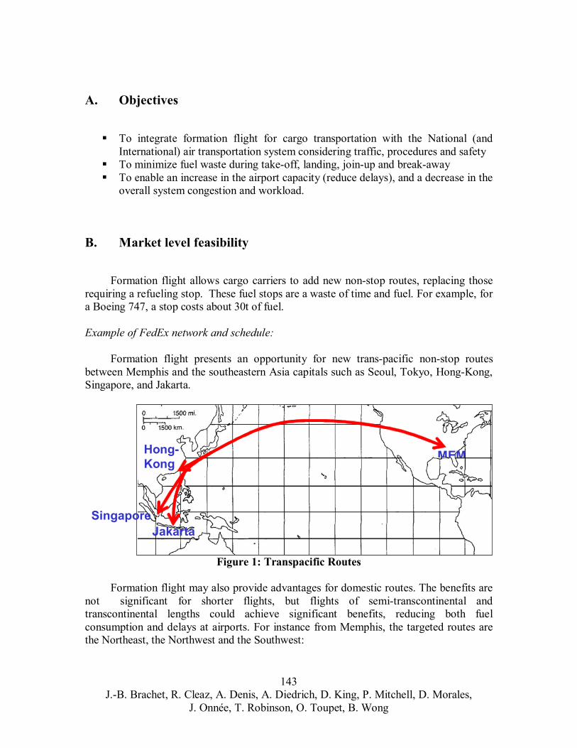
J.-B. Brachet, R. Cleaz, A. Denis, A. Diedrich, D. King, P. Mitchell, D. Morales, J. Onnée, T. Robinson, O. Toupet, B. Wong
143
A. Objectives
To integrate formation flight for cargo transportation with the National (and International) air transportation system considering traffic, procedures and safety To minimize fuel waste during take-off, landing, join-up and break-away To enable an increase in the airport capacity (reduce delays), and a decrease in the overall system congestion and workload.
B. Market level feasibility
Formation flight allows cargo carriers to add new non-stop routes, replacing those requiring a refueling stop. These fuel stops are a waste of time and fuel. For example, for a Boeing 747, a stop costs about 30t of fuel.
Example of FedEx network and schedule:
Formation flight presents an opportunity for new trans-pacific non-stop routes between Memphis and the southeastern Asia capitals such as Seoul, Tokyo, Hong-Kong, Singapore, and Jakarta.
MEMHong-Kong
JakartaSingapore
Figure 1: Transpacific Routes
Formation flight may also provide advantages for domestic routes. The benefits are not significant for shorter flights, but flights of semi-transcontinental and transcontinental lengths could achieve significant benefits, reducing both fuel consumption and delays at airports. For instance from Memphis, the targeted routes are the Northeast, the Northwest and the Southwest:
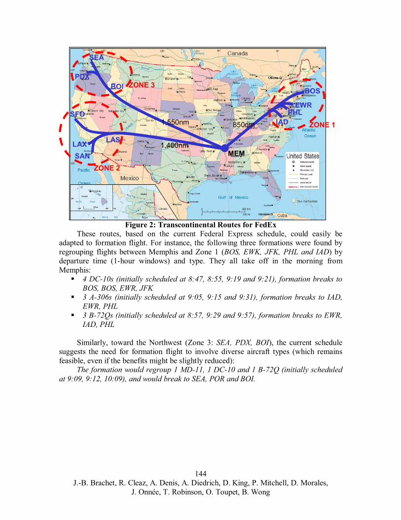
SEA
MEM
ZONE 1
ZONE 3
ZONE 2
IAD PHL
EWR
BOS
850nm
SAN LAX
SFO
LAS 1,400nm
PDX BOI
1,550nm
Figure 2: Transcontinental Routes for FedEx These routes, based on the current Federal Express schedule, could easily be
adapted to formation flight. For instance, the following three formations were found by regrouping flights between Memphis and Zone 1 (BOS, EWK, JFK, PHL and IAD) by departure time (1-hour windows) and type. They all take off in the morning from Memphis:
4 DC-10s (initially scheduled at 8:47, 8:55, 9:19 and 9:21), formation breaks to BOS, BOS, EWR, JFK 3 A-306s (initially scheduled at 9:05, 9:15 and 9:31), formation breaks to IAD, EWR, PHL 3 B-72Qs (initially scheduled at 8:57, 9:29 and 9:57), formation breaks to EWR, IAD, PHL
Similarly, toward the Northwest (Zone 3: SEA, PDX, BOI), the current schedule suggests the need for formation flight to involve diverse aircraft types (which remains feasible, even if the benefits might be slightly reduced):
The formation would regroup 1 MD-11, 1 DC-10 and 1 B-72Q (initially scheduled at 9:09, 9:12, 10:09), and would break to SEA, POR and BOI.
144 J.-B. Brachet, R. Cleaz, A. Denis, A. Diedrich, D. King, P. Mitchell, D. Morales,
J. Onnée, T. Robinson, O. Toupet, B. Wong
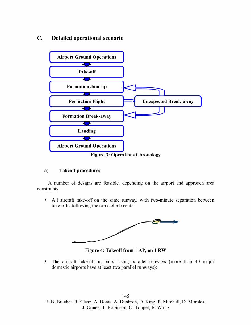
C. Detailed operational scenario
Airport Ground Operations
Take-off
Formation Join-up
Formation Flight
Formation Break-away
Landing
Airport Ground Operations
Unexpected Break-away
Figure 3: Operations Chronology
a) Takeoff procedures
A number of designs are feasible, depending on the airport and approach area constraints:
All aircraft take-off on the same runway, with two-minute separation between take-offs, following the same climb route:
Figure 4: Takeoff from 1 AP, on 1 RW
The aircraft take-off in pairs, using parallel runways (more than 40 major domestic airports have at least two parallel runways):
145 J.-B. Brachet, R. Cleaz, A. Denis, A. Diedrich, D. King, P. Mitchell, D. Morales,
J. Onnée, T. Robinson, O. Toupet, B. Wong
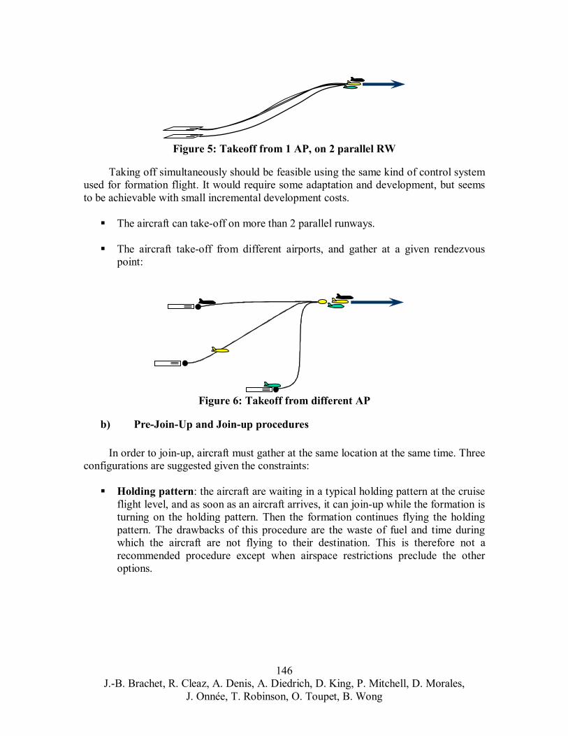
Figure 5: Takeoff from 1 AP, on 2 parallel RW
Taking off simultaneously should be feasible using the same kind of control system used for formation flight. It would require some adaptation and development, but seems to be achievable with small incremental development costs.
The aircraft can take-off on more than 2 parallel runways.
The aircraft take-off from different airports, and gather at a given rendezvous point:
Figure 6: Takeoff from different AP
b) Pre-Join-Up and Join-up procedures
In order to join-up, aircraft must gather at the same location at the same time. Three configurations are suggested given the constraints:
Holding pattern: the aircraft are waiting in a typical holding pattern at the cruise flight level, and as soon as an aircraft arrives, it can join-up while the formation is turning on the holding pattern. Then the formation continues flying the holding pattern. The drawbacks of this procedure are the waste of fuel and time during which the aircraft are not flying to their destination. This is therefore not a recommended procedure except when airspace restrictions preclude the other options.
146 J.-B. Brachet, R. Cleaz, A. Denis, A. Diedrich, D. King, P. Mitchell, D. Morales,
J. Onnée, T. Robinson, O. Toupet, B. Wong
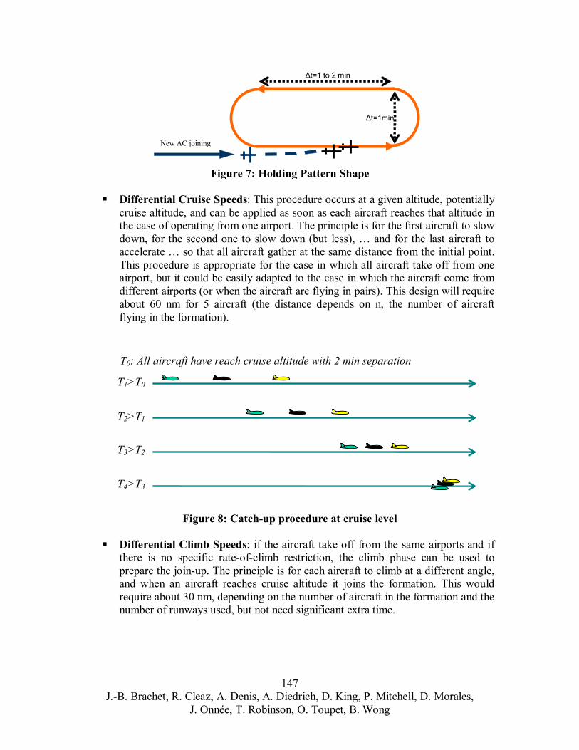
in
t=1min
t=1 to 2 m
New AC joining
Figure 7: Holding Pattern Shape
Differential Cruise Speeds: This procedure occurs at a given altitude, potentially cruise altitude, and can be applied as soon as each aircraft reaches that altitude in the case of operating from one airport. The principle is for the first aircraft to slow down, for the second one to slow down (but less), … and for the last aircraft to accelerate … so that all aircraft gather at the same distance from the initial point. This procedure is appropriate for the case in which all aircraft take off from one airport, but it could be easily adapted to the case in which the aircraft come from different airports (or when the aircraft are flying in pairs). This design will require about 60 nm for 5 aircraft (the distance depends on n, the number of aircraft flying in the formation).
T0: All aircraft have reach cruise altitude with 2 min separation
T3>T2
T4>T3
T1>T0
T2>T1
Figure 8: Catch-up procedure at cruise level
Differential Climb Speeds: if the aircraft take off from the same airports and if there is no specific rate-of-climb restriction, the climb phase can be used to prepare the join-up. The principle is for each aircraft to climb at a different angle, and when an aircraft reaches cruise altitude it joins the formation. This would require about 30 nm, depending on the number of aircraft in the formation and the number of runways used, but not need significant extra time.
147 J.-B. Brachet, R. Cleaz, A. Denis, A. Diedrich, D. King, P. Mitchell, D. Morales,
J. Onnée, T. Robinson, O. Toupet, B. Wong
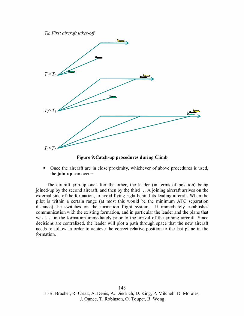
T0: First aircraft takes-off
T1>T0
T2>T1
T3>T2
Figure 9:Catch-up procedures during Climb
Once the aircraft are in close proximity, whichever of above procedures is used, the join-up can occur:
The aircraft join-up one after the other, the leader (in terms of position) being joined-up by the second aircraft, and then by the third … A joining aircraft arrives on the external side of the formation, to avoid flying right behind its leading aircraft. When the pilot is within a certain range (at most this would be the minimum ATC separation distance), he switches on the formation flight system. It immediately establishes communication with the existing formation, and in particular the leader and the plane that was last in the formation immediately prior to the arrival of the joining aircraft. Since decisions are centralized, the leader will plot a path through space that the new aircraft needs to follow in order to achieve the correct relative position to the last plane in the formation.
148 J.-B. Brachet, R. Cleaz, A. Denis, A. Diedrich, D. King, P. Mitchell, D. Morales,
J. Onnée, T. Robinson, O. Toupet, B. Wong

Figure 10: Join-up procedure in straight line
The military aircraft join up during a turn: the formation turns such that the external side of the formation is inside the curve and the joining aircraft will arrive inside the turn, with very little speed differential and no need to accelerate (taking advantage of the turn). If joining during a turn is required, the leader will coordinate a turn of the formation at the right time.
Figure 11: Join-up procedure during a turn
However, turning consumes more fuel and it would be more efficient to join-up in a straight line.
c) Rotation procedure
The rotation procedure is needed when the formation shape is the echelon. During cruise, when the aircraft are flying in formation, the aircraft rotate to maximize fuel savings and range. The rotations occur regularly, and the recommendation for their design is:
1
23. Slow down
4. C b
5. Descent
. Slight turn lim
. Catch-up
149 J.-B. Brachet, R. Cleaz, A. Denis, A. Diedrich, D. King, P. Mitchell, D. Morales,
J. Onnée, T. Robinson, O. Toupet, B. Wong
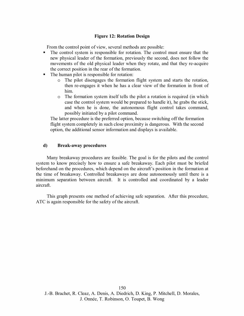
Figure 12: Rotation Design
From the control point of view, several methods are possible: The control system is responsible for rotation. The control must ensure that the new physical leader of the formation, previously the second, does not follow the movements of the old physical leader when they rotate, and that they re-acquire the correct position in the rear of the formation. The human pilot is responsible for rotation:
o The pilot disengages the formation flight system and starts the rotation, then re-engages it when he has a clear view of the formation in front of him.
o The formation system itself tells the pilot a rotation is required (in which case the control system would be prepared to handle it), he grabs the stick, and when he is done, the autonomous flight control takes command, possibly initiated by a pilot command.
The latter procedure is the preferred option, because switching off the formation flight system completely in such close proximity is dangerous. With the second option, the additional sensor information and displays is available.
d) Break-away procedures
Many breakaway procedures are feasible. The goal is for the pilots and the control system to know precisely how to ensure a safe breakaway. Each pilot must be briefed beforehand on the procedures, which depend on the aircraft’s position in the formation at the time of breakaway. Controlled breakaways are done autonomously until there is a minimum separation between aircraft. It is controlled and coordinated by a leader aircraft.
This graph presents one method of achieving safe separation. After this procedure, ATC is again responsible for the safety of the aircraft.
150 J.-B. Brachet, R. Cleaz, A. Denis, A. Diedrich, D. King, P. Mitchell, D. Morales,
J. Onnée, T. Robinson, O. Toupet, B. Wong
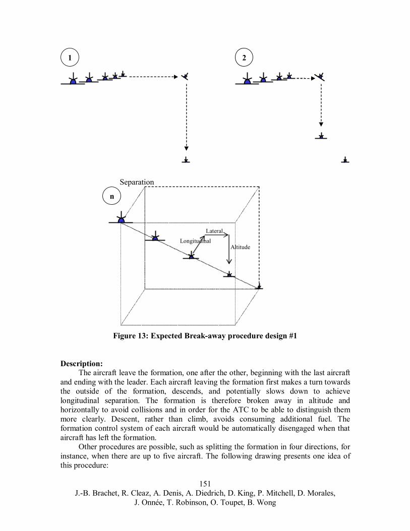
1 2
n
Separation
Longitudinal
Lateral
Altitude
Figure 13: Expected Break-away procedure design #1
Description: The aircraft leave the formation, one after the other, beginning with the last aircraft
and ending with the leader. Each aircraft leaving the formation first makes a turn towards the outside of the formation, descends, and potentially slows down to achieve longitudinal separation. The formation is therefore broken away in altitude and horizontally to avoid collisions and in order for the ATC to be able to distinguish them more clearly. Descent, rather than climb, avoids consuming additional fuel. The formation control system of each aircraft would be automatically disengaged when that aircraft has left the formation.
Other procedures are possible, such as splitting the formation in four directions, for instance, when there are up to five aircraft. The following drawing presents one idea of this procedure:
151 J.-B. Brachet, R. Cleaz, A. Denis, A. Diedrich, D. King, P. Mitchell, D. Morales,
J. Onnée, T. Robinson, O. Toupet, B. Wong
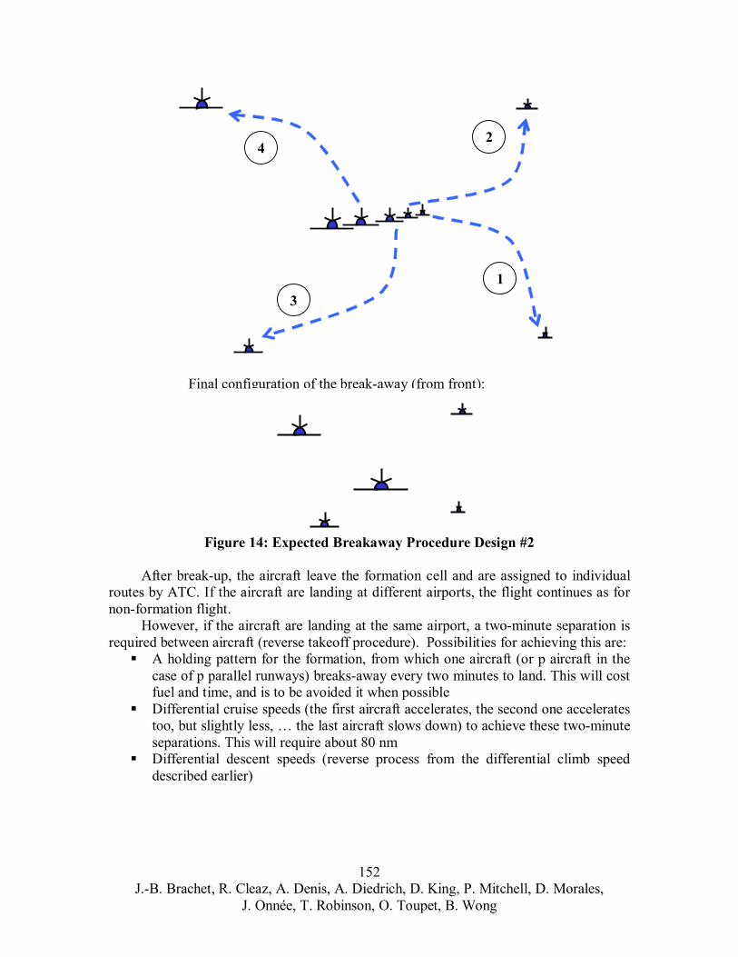
1
2
3
4
Final configuration of the break-away (from front):
Figure 14: Expected Breakaway Procedure Design #2
After break-up, the aircraft leave the formation cell and are assigned to individual routes by ATC. If the aircraft are landing at different airports, the flight continues as for non-formation flight.
However, if the aircraft are landing at the same airport, a two-minute separation is required between aircraft (reverse takeoff procedure). Possibilities for achieving this are:
A holding pattern for the formation, from which one aircraft (or p aircraft in the case of p parallel runways) breaks-away every two minutes to land. This will cost fuel and time, and is to be avoided it when possible Differential cruise speeds (the first aircraft accelerates, the second one accelerates too, but slightly less, … the last aircraft slows down) to achieve these two-minute separations. This will require about 80 nm Differential descent speeds (reverse process from the differential climb speed described earlier)
152 J.-B. Brachet, R. Cleaz, A. Denis, A. Diedrich, D. King, P. Mitchell, D. Morales,
J. Onnée, T. Robinson, O. Toupet, B. Wong
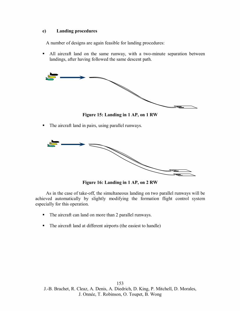
e) Landing procedures
A number of designs are again feasible for landing procedures:
All aircraft land on the same runway, with a two-minute separation between landings, after having followed the same descent path.
Figure 15: Landing in 1 AP, on 1 RW
The aircraft land in pairs, using parallel runways.
Figure 16: Landing in 1 AP, on 2 RW
As in the case of take-off, the simultaneous landing on two parallel runways will be achieved automatically by slightly modifying the formation flight control system especially for this operation.
The aircraft can land on more than 2 parallel runways.
The aircraft land at different airports (the easiest to handle)
153 J.-B. Brachet, R. Cleaz, A. Denis, A. Diedrich, D. King, P. Mitchell, D. Morales,
J. Onnée, T. Robinson, O. Toupet, B. Wong
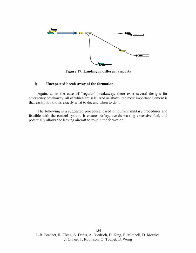
Figure 17: Landing in different airports
f) Unexpected break-away of the formation
Again, as in the case of “regular” breakaway, there exist several designs for emergency breakaway, all of which are safe. And as above, the most important element is that each pilot knows exactly what to do, and when to do it.
The following is a suggested procedure, based on current military procedures and feasible with the control system. It ensures safety, avoids wasting excessive fuel, and potentially allows the leaving aircraft to re-join the formation:
154 J.-B. Brachet, R. Cleaz, A. Denis, A. Diedrich, D. King, P. Mitchell, D. Morales,
J. Onnée, T. Robinson, O. Toupet, B. Wong
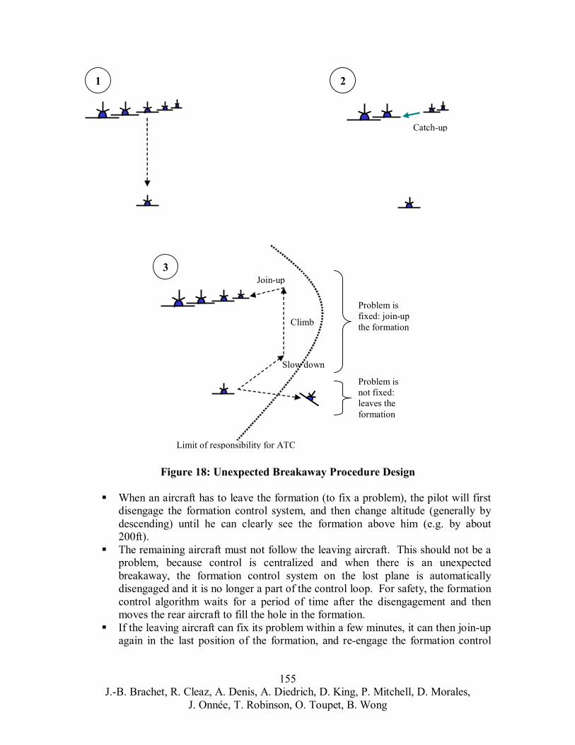
1 2
pCatch-u
p
p y
3
Slow down
Climb
Join-u
Limit of res onsibilit for ATC
Problem is fixed: join-up the formation
Problem is not fixed: leaves the formation
Figure 18: Unexpected Breakaway Procedure Design
When an aircraft has to leave the formation (to fix a problem), the pilot will first disengage the formation control system, and then change altitude (generally by descending) until he can clearly see the formation above him (e.g. by about 200ft). The remaining aircraft must not follow the leaving aircraft. This should not be a problem, because control is centralized and when there is an unexpected breakaway, the formation control system on the lost plane is automatically disengaged and it is no longer a part of the control loop. For safety, the formation control algorithm waits for a period of time after the disengagement and then moves the rear aircraft to fill the hole in the formation. If the leaving aircraft can fix its problem within a few minutes, it can then join-up again in the last position of the formation, and re-engage the formation control
155 J.-B. Brachet, R. Cleaz, A. Denis, A. Diedrich, D. King, P. Mitchell, D. Morales,
J. Onnée, T. Robinson, O. Toupet, B. Wong
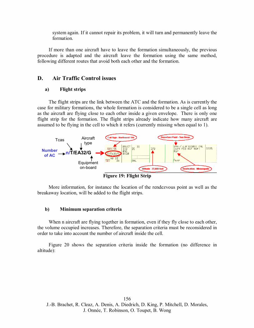
system again. If it cannot repair its problem, it will turn and permanently leave the formation.
If more than one aircraft have to leave the formation simultaneously, the previous procedure is adapted and the aircraft leave the formation using the same method, following different routes that avoid both each other and the formation.
D. Air Traffic Control issues
a) Flight strips
The flight strips are the link between the ATC and the formation. As is currently the case for military formations, the whole formation is considered to be a single cell as long as the aircraft are flying close to each other inside a given envelope. There is only one flight strip for the formation. The flight strips already indicate how many aircraft are assumed to be flying in the cell to which it refers (currently missing when equal to 1).
Tcas Aircraft type
Number of AC
n/T/EA32/G
Equipment on-board
Figure 19: Flight Strip
More information, for instance the location of the rendezvous point as well as the breakaway location, will be added to the flight strips.
b) Minimum separation criteria
When n aircraft are flying together in formation, even if they fly close to each other, the volume occupied increases. Therefore, the separation criteria must be reconsidered in order to take into account the number of aircraft inside the cell.
Figure 20 shows the separation criteria inside the formation (no difference in altitude):
156 J.-B. Brachet, R. Cleaz, A. Denis, A. Diedrich, D. King, P. Mitchell, D. Morales,
J. Onnée, T. Robinson, O. Toupet, B. Wong
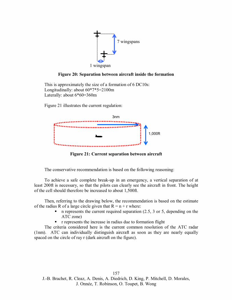
7 wingspans
1 wingspan
Figure 20: Separation between aircraft inside the formation
This is approximately the size of a formation of 6 DC10s: Longitudinally: about 60*7*5=2100m Laterally: about 6*60=360m
Figure 21 illustrates the current regulation:
3nm
1,000ft
Figure 21: Current separation between aircraft
The conservative recommendation is based on the following reasoning:
To achieve a safe complete break-up in an emergency, a vertical separation of at least 200ft is necessary, so that the pilots can clearly see the aircraft in front. The height of the cell should therefore be increased to about 1,500ft.
Then, referring to the drawing below, the recommendation is based on the estimate of the radius R of a large circle given that R = n + r where:
n represents the current required separation (2.5, 3 or 5, depending on the ATC zone) r represents the increase in radius due to formation flight
The criteria considered here is the current common resolution of the ATC radar (1nm). ATC can individually distinguish aircraft as soon as they are nearly equally spaced on the circle of ray r (dark aircraft on the figure).
157 J.-B. Brachet, R. Cleaz, A. Denis, A. Diedrich, D. King, P. Mitchell, D. Morales,
J. Onnée, T. Robinson, O. Toupet, B. Wong
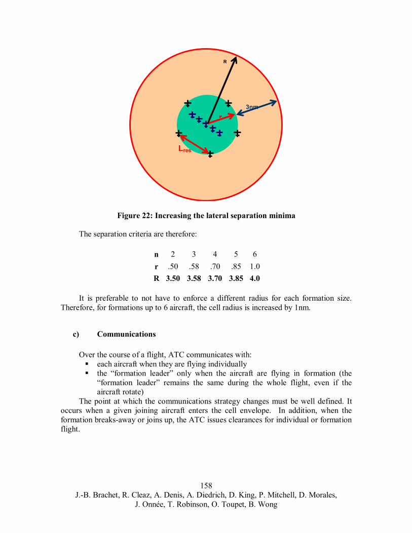
L
r3nm
R
res
Figure 22: Increasing the lateral separation minima
The separation criteria are therefore:
n 2 3 4 5 6r .50 .58 .70 .85 1.0 R 3.50 3.58 3.70 3.85 4.0
It is preferable to not have to enforce a different radius for each formation size. Therefore, for formations up to 6 aircraft, the cell radius is increased by 1nm.
c) Communications
Over the course of a flight, ATC communicates with: each aircraft when they are flying individually the “formation leader” only when the aircraft are flying in formation (the “formation leader” remains the same during the whole flight, even if the aircraft rotate)
The point at which the communications strategy changes must be well defined. It occurs when a given joining aircraft enters the cell envelope. In addition, when the formation breaks-away or joins up, the ATC issues clearances for individual or formation flight.
158 J.-B. Brachet, R. Cleaz, A. Denis, A. Diedrich, D. King, P. Mitchell, D. Morales,
J. Onnée, T. Robinson, O. Toupet, B. Wong
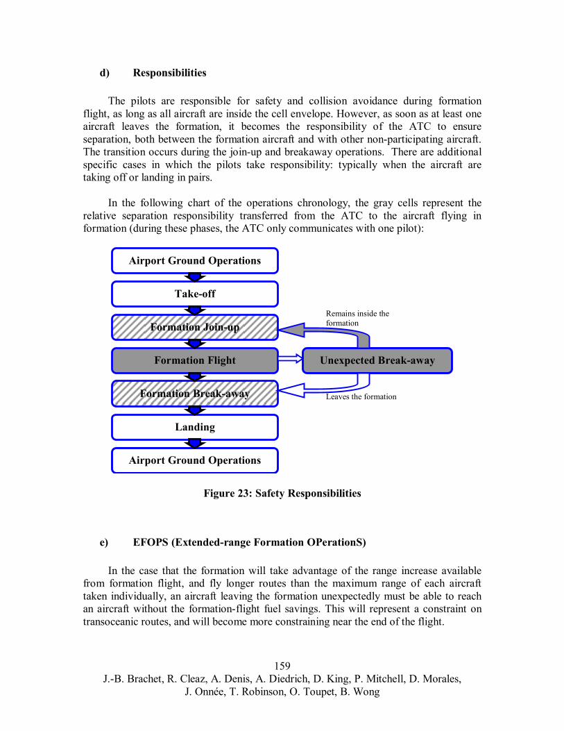
d) Responsibilities
The pilots are responsible for safety and collision avoidance during formation flight, as long as all aircraft are inside the cell envelope. However, as soon as at least one aircraft leaves the formation, it becomes the responsibility of the ATC to ensure separation, both between the formation aircraft and with other non-participating aircraft. The transition occurs during the join-up and breakaway operations. There are additional specific cases in which the pilots take responsibility: typically when the aircraft are taking off or landing in pairs.
In the following chart of the operations chronology, the gray cells represent the relative separation responsibility transferred from the ATC to the aircraft flying in formation (during these phases, the ATC only communicates with one pilot):
Airport Ground Operations
Take-off
Formation Join-up
Formation Flight
Formation Break-away
Landing
Airport Ground Operations
Unexpected Break-away
Remains inside the formation
Leaves the formation
Figure 23: Safety Responsibilities
e) EFOPS (Extended-range Formation OPerationS)
In the case that the formation will take advantage of the range increase available from formation flight, and fly longer routes than the maximum range of each aircraft taken individually, an aircraft leaving the formation unexpectedly must be able to reach an aircraft without the formation-flight fuel savings. This will represent a constraint on transoceanic routes, and will become more constraining near the end of the flight.
159 J.-B. Brachet, R. Cleaz, A. Denis, A. Diedrich, D. King, P. Mitchell, D. Morales,
J. Onnée, T. Robinson, O. Toupet, B. Wong

E. Overall system capacity improvement and decrease in ATC workload
Formation flight can increase the airspace capacity and decrease the air traffic control workload, leading to benefits for both air carriers and the air transportation system.
a) Airport capacity increases
When the aircraft are taking off from the same airport and when the airport owns at least two parallel runways, it will be possible, after additional development of the formation flight control system, to take off and land simultaneously in pairs. When applied to the hub of a cargo airline using formation flight, this should significantly decrease airport delays at peak times.
b) National Airspace capacity enhancement
The following map considers a few routes on which formation flight could be used by Federal Express (departing from Memphis), and shows the en-route divisions of the domestic airspace.
ZB
ZNZOZA
ZM
ZM
ZK ZI
ZD
ZT
ZJ
ZM
ZF
ZD
ZL
ZH
ZS
ZO
ZLZA ME
Figure 24: Formation Flight over the National Airspace main divisions
The formations will fly over at least 3 zones in each case. Especially in the zones where formations are neither joining-up, nor breaking-away, ATC will take advantage of the “1 formation = 1 cell” concept and be able to handle more airplanes simultaneously. When the zone is congested, this will increase the allowable traffic.
160 J.-B. Brachet, R. Cleaz, A. Denis, A. Diedrich, D. King, P. Mitchell, D. Morales,
J. Onnée, T. Robinson, O. Toupet, B. Wong
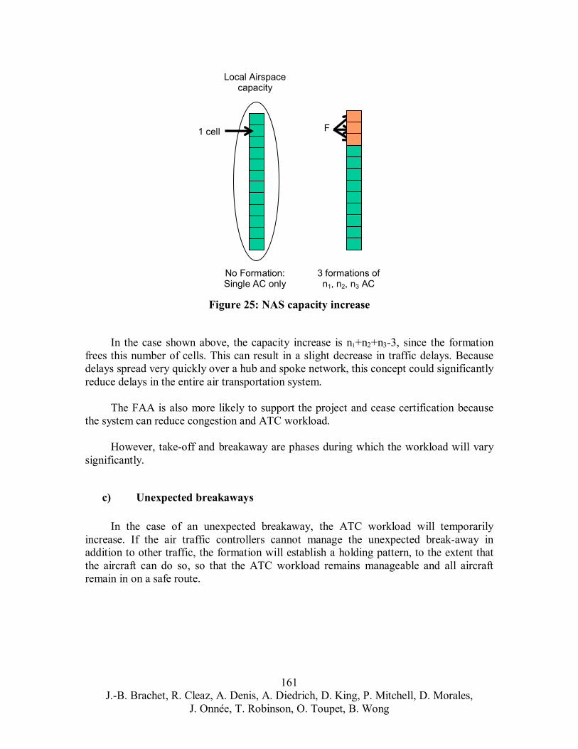
Local Airspace capacity
F1 cell
No Formation: 3 formations of Single AC only n1, n2, n3 AC
Figure 25: NAS capacity increase
In the case shown above, the capacity increase is n1+n2+n3-3, since the formation frees this number of cells. This can result in a slight decrease in traffic delays. Because delays spread very quickly over a hub and spoke network, this concept could significantly reduce delays in the entire air transportation system.
The FAA is also more likely to support the project and cease certification because the system can reduce congestion and ATC workload.
However, take-off and breakaway are phases during which the workload will vary significantly.
c) Unexpected breakaways
In the case of an unexpected breakaway, the ATC workload will temporarily increase. If the air traffic controllers cannot manage the unexpected break-away in addition to other traffic, the formation will establish a holding pattern, to the extent that the aircraft can do so, so that the ATC workload remains manageable and all aircraft remain in on a safe route.
161 J.-B. Brachet, R. Cleaz, A. Denis, A. Diedrich, D. King, P. Mitchell, D. Morales,
J. Onnée, T. Robinson, O. Toupet, B. Wong
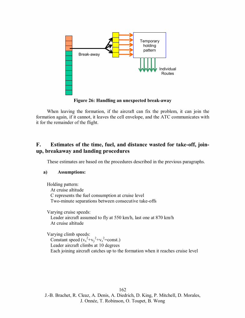
idual
Break-away
Temporary holding pattern
IndivRoutes
Figure 26: Handling an unexpected break-away
When leaving the formation, if the aircraft can fix the problem, it can join the formation again, if it cannot, it leaves the cell envelope, and the ATC communicates with it for the remainder of the flight.
F. Estimates of the time, fuel, and distance wasted for take-off, join-up, breakaway and landing procedures
These estimates are based on the procedures described in the previous paragraphs.
a) Assumptions:
Holding pattern: At cruise altitude C represents the fuel consumption at cruise level Two-minute separations between consecutive take-offs
Varying cruise speeds: Leader aircraft assumed to fly at 550 km/h, last one at 870 km/h At cruise altitude
Varying climb speeds: Constant speed (vx
2+vy2+vz
2=const.) Leader aircraft climbs at 10 degrees Each joining aircraft catches up to the formation when it reaches cruise level
162 J.-B. Brachet, R. Cleaz, A. Denis, A. Diedrich, D. King, P. Mitchell, D. Morales,
J. Onnée, T. Robinson, O. Toupet, B. Wong
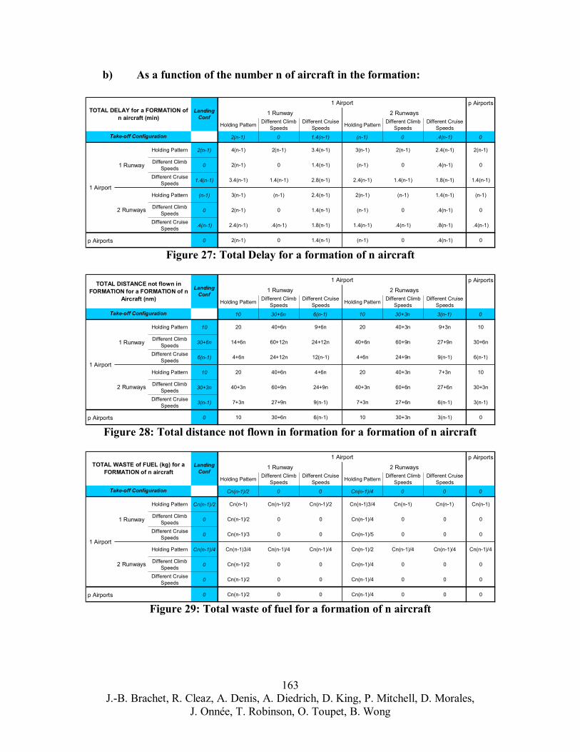
J.-B. Brachet, R. Cleaz, A. Denis, A. Diedrich, D. King, P. Mitchell, D. Morales, J. Onnée, T. Robinson, O. Toupet, B. Wong
163
b) As a function of the number n of aircraft in the formation:
p Airports
Holding Pattern Different Climb Speeds
Different Cruise Speeds Holding Pattern Different Climb
SpeedsDifferent Cruise
Speeds
2(n-1) 0 1.4(n-1) (n-1) 0 .4(n-1) 0
Holding Pattern 2(n-1) 4(n-1) 2(n-1) 3.4(n-1) 3(n-1) 2(n-1) 2.4(n-1) 2(n-1)
Different Climb Speeds 0 2(n-1) 0 1.4(n-1) (n-1) 0 .4(n-1) 0
Different Cruise Speeds 1.4(n-1) 3.4(n-1) 1.4(n-1) 2.8(n-1) 2.4(n-1) 1.4(n-1) 1.8(n-1) 1.4(n-1)
Holding Pattern (n-1) 3(n-1) (n-1) 2.4(n-1) 2(n-1) (n-1) 1.4(n-1) (n-1)
Different Climb Speeds 0 2(n-1) 0 1.4(n-1) (n-1) 0 .4(n-1) 0
Different Cruise Speeds .4(n-1) 2.4(n-1) .4(n-1) 1.8(n-1) 1.4(n-1) .4(n-1) .8(n-1) .4(n-1)
p Airports 0 2(n-1) 0 1.4(n-1) (n-1) 0 .4(n-1) 0
TOTAL DELAY for a FORMATION of n aircraft (min)
Landing Conf
1 Airport
1 Runway 2 Runways
Take-off Configuration
1 Airport
1 Runway
2 Runways
Figure 27: Total Delay for a formation of n aircraft
p Airports
Holding Pattern Different Climb Speeds
Different Cruise Speeds Holding Pattern Different Climb
SpeedsDifferent Cruise
Speeds
10 30+6n 6(n-1) 10 30+3n 3(n-1) 0
Holding Pattern 10 20 40+6n 9+6n 20 40+3n 9+3n 10
Different Climb Speeds 30+6n 14+6n 60+12n 24+12n 40+6n 60+9n 27+9n 30+6n
Different Cruise Speeds 6(n-1) 4+6n 24+12n 12(n-1) 4+6n 24+9n 9(n-1) 6(n-1)
Holding Pattern 10 20 40+6n 4+6n 20 40+3n 7+3n 10
Different Climb Speeds 30+3n 40+3n 60+9n 24+9n 40+3n 60+6n 27+6n 30+3n
Different Cruise Speeds 3(n-1) 7+3n 27+9n 9(n-1) 7+3n 27+6n 6(n-1) 3(n-1)
p Airports 0 10 30+6n 6(n-1) 10 30+3n 3(n-1) 0
Take-off Configuration
1 Airport
1 Runway
2 Runways
TOTAL DISTANCE not flown in FORMATION for a FORMATION of n
Aircraft (nm)
Landing Conf
1 Airport
1 Runway 2 Runways
Figure 28: Total distance not flown in formation for a formation of n aircraft
p Airports
Holding Pattern Different Climb Speeds
Different Cruise Speeds Holding Pattern Different Climb
SpeedsDifferent Cruise
Speeds
Cn(n-1)/2 0 0 Cn(n-1)/4 0 0 0
Holding Pattern Cn(n-1)/2 Cn(n-1) Cn(n-1)/2 Cn(n-1)/2 Cn(n-1)3/4 Cn(n-1) Cn(n-1) Cn(n-1)
Different Climb Speeds 0 Cn(n-1)/2 0 0 Cn(n-1)/4 0 0 0
Different Cruise Speeds 0 Cn(n-1)/3 0 0 Cn(n-1)/5 0 0 0
Holding Pattern Cn(n-1)/4 Cn(n-1)3/4 Cn(n-1)/4 Cn(n-1)/4 Cn(n-1)/2 Cn(n-1)/4 Cn(n-1)/4 Cn(n-1)/4
Different Climb Speeds 0 Cn(n-1)/2 0 0 Cn(n-1)/4 0 0 0
Different Cruise Speeds 0 Cn(n-1)/2 0 0 Cn(n-1)/4 0 0 0
p Airports 0 Cn(n-1)/2 0 0 Cn(n-1)/4 0 0 0
TOTAL WASTE of FUEL (kg) for a FORMATION of n aircraft
Landing Conf
1 Airport
1 Runway 2 Runways
Take-off Configuration
1 Airport
1 Runway
2 Runways
Figure 29: Total waste of fuel for a formation of n aircraft

J.-B. Brachet, R. Cleaz, A. Denis, A. Diedrich, D. King, P. Mitchell, D. Morales, J. Onnée, T. Robinson, O. Toupet, B. Wong
164
c) Example of a formation of 5 DC10s:
p Airports
Holding Pattern Different Climb Speeds
Different Cruise Speeds Holding Pattern Different Climb
SpeedsDifferent Cruise
Speeds
8 0 4.75 4 0 2.5 0
Holding Pattern 8 16 8 12.75 12 8 10.5 8
Different Climb Speeds 0 8 0 4.75 4 0 2.5 0
Different Cruise Speeds 4.75 12.75 4.75 9.5 8.75 4.75 7.25 4.75
Holding Pattern 4 12 4 8.75 8 4 6.5 4
Different Climb Speeds 0 8 0 4.75 4 0 2.5 0
Different Cruise Speeds 2.5 10.5 2.5 7.25 6.5 2.5 5 2.5
p Airports 0 8 0 4.75 4 0 2.5 0
1 Airport
1 Runway 2 Runways
1 Runway
2 Runways
1 Airport
Landing Conf
Take-off Configuration
TOTAL DELAY for a FORMATION of 5 DC-10 (min)
Figure 30: Total delay for a formation of 5 DC10
p Airports
Holding Pattern Different Climb Speeds
Different Cruise Speeds Holding Pattern Different Climb
SpeedsDifferent Cruise
Speeds
10 60 24 10 60 12 0
Holding Pattern 10 20 70 34 20 70 22 10
Different Climb Speeds 60 70 120 84 70 120 72 60
Different Cruise Speeds 24 34 84 48 34 84 36 24
Holding Pattern 10 20 70 34 20 70 22 10
Different Climb Speeds 60 70 120 84 70 120 72 60
Different Cruise Speeds 12 22 72 36 22 72 24 12
p Airports 0 10 60 24 10 60 12 0
1 Airport
1 Runway 2 Runways
1 Runway
2 Runways
1 Airport
Landing Conf
Take-off Configuration
TOTAL DISTANCE not flown in FORMATION for a FORMATION of 5
Aircraft (nm)
Figure 31: Total distance not flown in formation for a formation of 5 DC10
p Airports
Holding Pattern Different Climb Speeds
Different Cruise Speeds Holding Pattern Different Climb
SpeedsDifferent Cruise
Speeds
Cn(n-1)/2 0 0 Cn(n-1)/4 0 0 0
Holding Pattern Cn(n-1)/2 Cn(n-1) Cn(n-1)/2 Cn(n-1)/2 Cn(n-1)3/4 Cn(n-1) Cn(n-1) Cn(n-1)
Different Climb Speeds 0 Cn(n-1)/2 0 0 Cn(n-1)/4 0 0 0
Different Cruise Speeds 0 Cn(n-1)/3 0 0 Cn(n-1)/5 0 0 0
Holding Pattern Cn(n-1)/4 Cn(n-1)3/4 Cn(n-1)/4 Cn(n-1)/4 Cn(n-1)/2 Cn(n-1)/4 Cn(n-1)/4 Cn(n-1)/4
Different Climb Speeds 0 Cn(n-1)/2 0 0 Cn(n-1)/4 0 0 0
Different Cruise Speeds 0 Cn(n-1)/2 0 0 Cn(n-1)/4 0 0 0
p Airports 0 Cn(n-1)/2 0 0 Cn(n-1)/4 0 0 0
TOTAL WASTE of FUEL (kg) for a FORMATION of n aircraft
Landing Conf
1 Airport
1 Runway 2 Runways
Take-off Configuration
1 Airport
1 Runway
2 Runways
Figure 32: Total waste of fuel for a formation of 5 DC10

Acknowledgement
J. Hansman J.P. Clarke M. Cummings R. Holmes
References
Paul Jackson, “All the World Aircraft”, Jane’s Information Group: 01 July 2003 (ISBN: 0710625375) Eurocontrol DABA 3.3: 2003 (Data Base) ETMS Data Base: 11 Jan 2003 Federal Aviation Administration (FAA) Internet site (http://www.faa.gov)
165 J.-B. Brachet, R. Cleaz, A. Denis, A. Diedrich, D. King, P. Mitchell, D. Morales,
J. Onnée, T. Robinson, O. Toupet, B. Wong

XV. System Safety
166 J.-B. Brachet, R. Cleaz, A. Denis, A. Diedrich, D. King, P. Mitchell, D. Morales,
J. Onnée, T. Robinson, O. Toupet, B. Wong
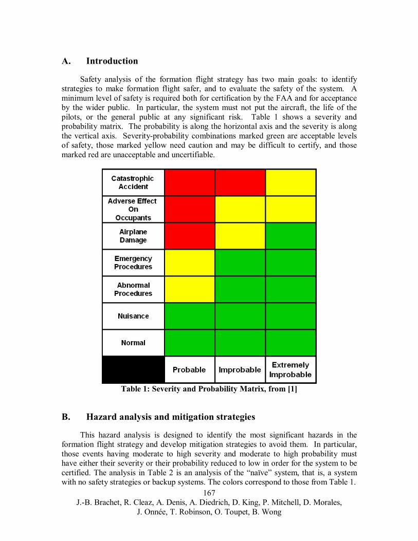
A. Introduction
Safety analysis of the formation flight strategy has two main goals: to identify strategies to make formation flight safer, and to evaluate the safety of the system. A minimum level of safety is required both for certification by the FAA and for acceptance by the wider public. In particular, the system must not put the aircraft, the life of the pilots, or the general public at any significant risk. Table 1 shows a severity and probability matrix. The probability is along the horizontal axis and the severity is along the vertical axis. Severity-probability combinations marked green are acceptable levels of safety, those marked yellow need caution and may be difficult to certify, and those marked red are unacceptable and uncertifiable.
Table 1: Severity and Probability Matrix, from [1]
B. Hazard analysis and mitigation strategies
This hazard analysis is designed to identify the most significant hazards in the formation flight strategy and develop mitigation strategies to avoid them. In particular, those events having moderate to high severity and moderate to high probability must have either their severity or their probability reduced to low in order for the system to be certified. The analysis in Table 2 is an analysis of the “naïve” system, that is, a system with no safety strategies or backup systems. The colors correspond to those from Table 1.
167 J.-B. Brachet, R. Cleaz, A. Denis, A. Diedrich, D. King, P. Mitchell, D. Morales,
J. Onnée, T. Robinson, O. Toupet, B. Wong
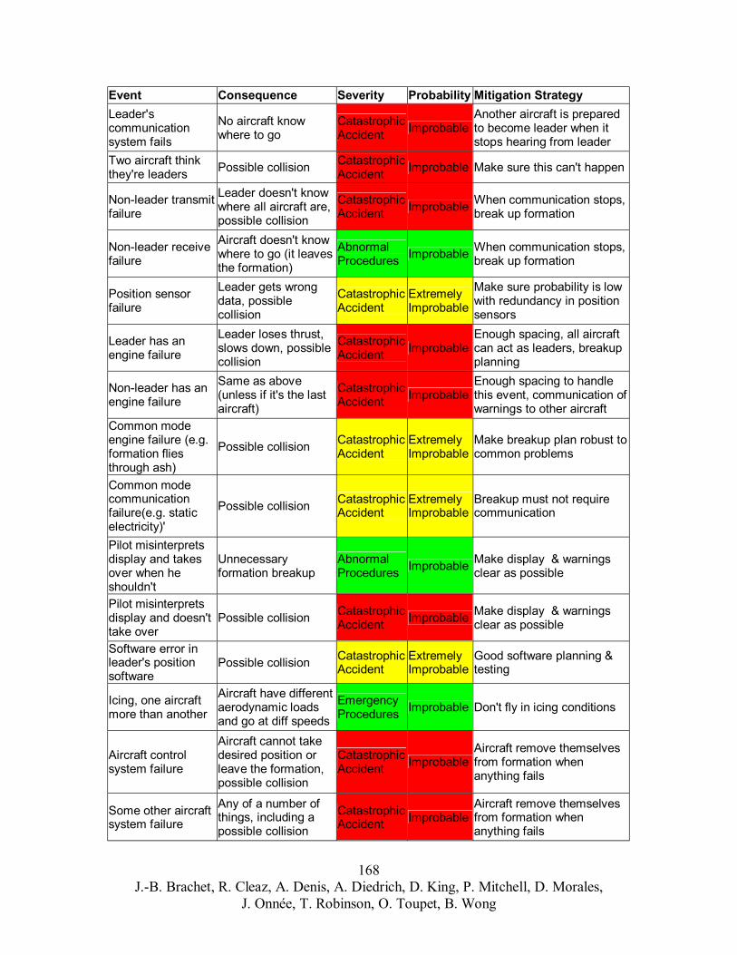
i ion fails ident
il
i leader i
ident i
Non-l it li ion ident
i iion
Non-l Aiit l
ion)
l i iion
iti i ident
li is lwi i ition
Leader lsl i ident
i l
Non-l ( i lai ) ident
ii i i
i i
(ion fli ident
i ion ic
ici )' ident i ion
Pil isil
il l ings
cl i
Pil isil ident
l ings cl i
in l ition sof ident ing
i Ai iic loads ly in ici ions
lAidesi ition or l ion,
i ion ident
li
i
i i i luding a i ion ident
li
i
Event Consequence Severity Probability Mitigation Strategy Leader's commun catsystem
No aircraft know where to go
Catastrophic Acc Improbable
Another aircraft s prepared to become eader when it stops hear ng from
Two aircraft th nk they're leaders Possible collision Catastrophic
Acc Improbable Make sure th s can't happen
eader transmfailure
Leader doesn't know where al aircraft are, poss ble collis
Catastrophic Acc Improbable When commun cat on stops,
break up format
eader receive failure
rcraft doesn't know where to go ( eaves the format
AbnormaProcedures Improbable When commun cat on stops,
break up format
Pos on sensor failure
Leader gets wrong data, poss ble collision
Catastrophic Acc
Extremely Improbable
Make sure probabi ty ow th redundancy n pos
sensors
Leader has an engine failure
oses thrust, ows down, poss ble
collision
Catastrophic Acc Improbable
Enough spac ng, all aircraft can act as eaders, breakup planning
eader has an engine failure
Same as above unless f it's the ast rcraft
Catastrophic Acc Improbable
Enough spac ng to handle th s event, commun cat on of warn ngs to other a rcraft
Common mode engine failure e.g. format es through ash)
Possible collision Catastrophic Acc
Extremely Improbable
Make breakup plan robust to common problems
Common mode commun catfailure(e.g. statelectr ty
Possible collision Catastrophic Acc
Extremely Improbable
Breakup must not require commun cat
ot m nterprets disp ay and takes over when he shouldn't
Unnecessary format on breakup
AbnormaProcedures Improbable Make disp ay & warn
ear as poss ble
ot m nterprets disp ay and doesn't take over
Possible collision Catastrophic Acc Improbable Make disp ay & warn
ear as poss ble
Software erroreader's pos
tware Possible collision Catastrophic
AccExtremely Improbable
Good software planning & test
Ic ng, one aircraft more than another
rcraft have d fferent aerodynamand go at diff speeds
Emergency Procedures Improbable Don't f ng condit
Aircraft controsystem failure
rcraft cannot take red pos
eave the formatposs ble collis
Catastrophic Acc Improbable
Aircraft remove themse ves from format on when anyth ng fails
Some other a rcraft system failure
Any of a number of th ngs, ncposs ble collis
Catastrophic Acc Improbable
Aircraft remove themse ves from format on when anyth ng fails
168 J.-B. Brachet, R. Cleaz, A. Denis, A. Diedrich, D. King, P. Mitchell, D. Morales,
J. Onnée, T. Robinson, O. Toupet, B. Wong
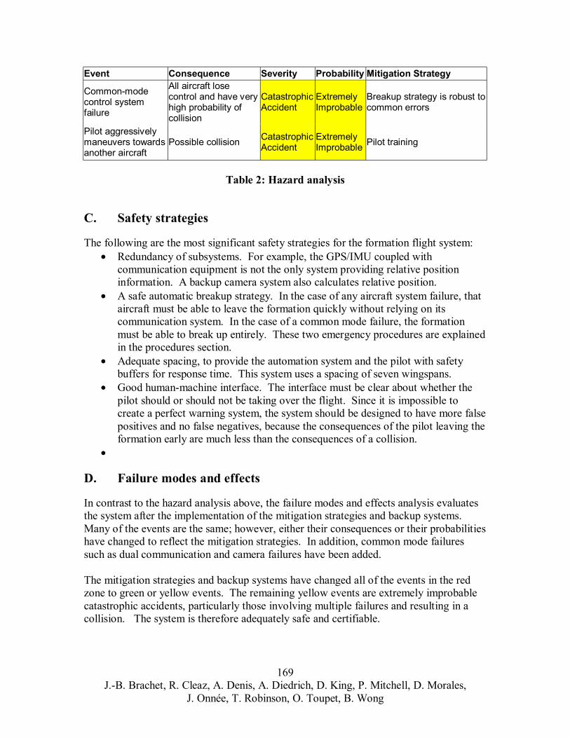
Event Consequence Severity Probability Mitigation Strategy
Common-mode control system failure
Pilot aggressively maneuvers towards another aircraft
All aircraft lose control and have very high probability of collision
Possible collision
Catastrophic Accident
Catastrophic Accident
Extremely Improbable
Extremely Improbable
Breakup strategy is robust to common errors
Pilot training
Table 2: Hazard analysis
C. Safety strategies
The following are the most significant safety strategies for the formation flight system: • Redundancy of subsystems. For example, the GPS/IMU coupled with
communication equipment is not the only system providing relative position information. A backup camera system also calculates relative position.
• A safe automatic breakup strategy. In the case of any aircraft system failure, that aircraft must be able to leave the formation quickly without relying on its communication system. In the case of a common mode failure, the formation must be able to break up entirely. These two emergency procedures are explained in the procedures section.
• Adequate spacing, to provide the automation system and the pilot with safety buffers for response time. This system uses a spacing of seven wingspans.
• Good human-machine interface. The interface must be clear about whether the pilot should or should not be taking over the flight. Since it is impossible to create a perfect warning system, the system should be designed to have more false positives and no false negatives, because the consequences of the pilot leaving the formation early are much less than the consequences of a collision.
•
D. Failure modes and effects
In contrast to the hazard analysis above, the failure modes and effects analysis evaluates the system after the implementation of the mitigation strategies and backup systems. Many of the events are the same; however, either their consequences or their probabilities have changed to reflect the mitigation strategies. In addition, common mode failures such as dual communication and camera failures have been added.
The mitigation strategies and backup systems have changed all of the events in the red zone to green or yellow events. The remaining yellow events are extremely improbable catastrophic accidents, particularly those involving multiple failures and resulting in a collision. The system is therefore adequately safe and certifiable.
169 J.-B. Brachet, R. Cleaz, A. Denis, A. Diedrich, D. King, P. Mitchell, D. Morales,
J. Onnée, T. Robinson, O. Toupet, B. Wong
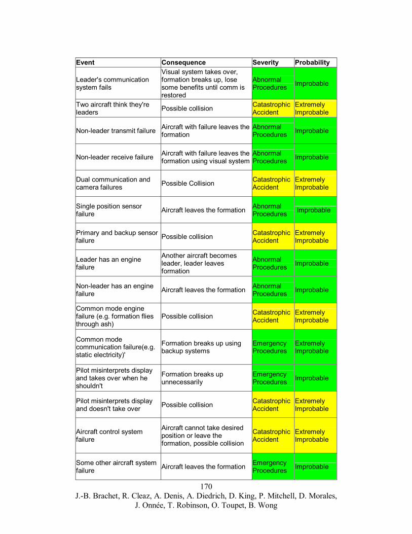
i ion fails
Vi li l
i is l
il ident
Non-l i il Ai iion
l
Non-l Ai iion usi i
l
i ion and il ibl ion ident
Si iti Ai l ion l
ident
l leader lion
l
Non-l Ai l ion l
( ion fli ident
i il )'
i ing
Pil isi l iily
Pil isi lident
l Ai iposition or l
i i llision ident
i Ai l ion
Event Consequence Severity Probability
Leader's commun catsystem
sua system takes over, format on breaks up, ose some benef ts until comm restored
AbnormaProcedures Improbable
Two aircraft th nk they're eaders Possible collision Catastrophic
AccExtremely Improbable
eader transm t fa ure rcraft w th failure leaves the format
AbnormaProcedures Improbable
eader receive failure rcraft w th failure leaves the format ng v sual system
AbnormaProcedures Improbable
Dual commun catcamera fa ures Poss e Collis Catastrophic
AccExtremely Improbable
ngle pos on sensor failure rcraft eaves the format Abnorma
Procedures Improbable
Primary and backup sensor failure Possible collision Catastrophic
AccExtremely Improbable
Leader has an engine failure
Another aircraft becomes eader, eaves format
AbnormaProcedures Improbable
eader has an engine failure rcraft eaves the format Abnorma
Procedures Improbable
Common mode engine failure e.g. format es through ash)
Possible collision Catastrophic Acc
Extremely Improbable
Common mode commun cat on failure(e.g. static e ectricity
Format on breaks up usbackup systems
Emergency Procedures
Extremely Improbable
ot m nterprets disp ay and takes over when he shouldn't
Format on breaks up unnecessar
Emergency Procedures Improbable
ot m nterprets disp ay and doesn't take over Possible collision Catastrophic
AccExtremely Improbable
Aircraft contro system failure
rcraft cannot take des red eave the
format on, poss ble co
Catastrophic Acc
Extremely Improbable
Some other a rcraft system failure rcraft eaves the format Emergency
Procedures Improbable
170 J.-B. Brachet, R. Cleaz, A. Denis, A. Diedrich, D. King, P. Mitchell, D. Morales,
J. Onnée, T. Robinson, O. Toupet, B. Wong
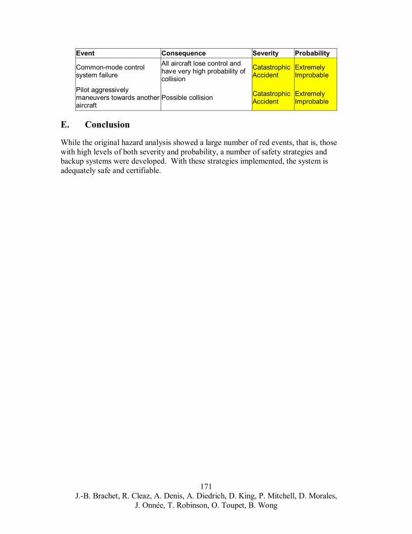
Event Consequence Severity Probability
Common-mode control system failure
Pilot aggressively maneuvers towards another aircraft
All aircraft lose control and have very high probability of collision
Possible collision
Catastrophic Accident
Catastrophic Accident
Extremely Improbable
Extremely Improbable
E. Conclusion
While the original hazard analysis showed a large number of red events, that is, those with high levels of both severity and probability, a number of safety strategies and backup systems were developed. With these strategies implemented, the system is adequately safe and certifiable.
171 J.-B. Brachet, R. Cleaz, A. Denis, A. Diedrich, D. King, P. Mitchell, D. Morales,
J. Onnée, T. Robinson, O. Toupet, B. Wong

References
[1] R.J. Hansman, Safety, Reliability, Certification, Maintenance, lecture, 16.885 class, Massachusetts Institute of Technology, November 18th, 2003
172 J.-B. Brachet, R. Cleaz, A. Denis, A. Diedrich, D. King, P. Mitchell, D. Morales,
J. Onnée, T. Robinson, O. Toupet, B. Wong

173 J.-B. Brachet, R. Cleaz, A. Denis, A. Diedrich, D. King, P. Mitchell, D. Morales,
J. Onnée, T. Robinson, O. Toupet, B. Wong

XVI. Program Risk Analysis and Risk Reduction
174 J.-B. Brachet, R. Cleaz, A. Denis, A. Diedrich, D. King, P. Mitchell, D. Morales,
J. Onnée, T. Robinson, O. Toupet, B. Wong
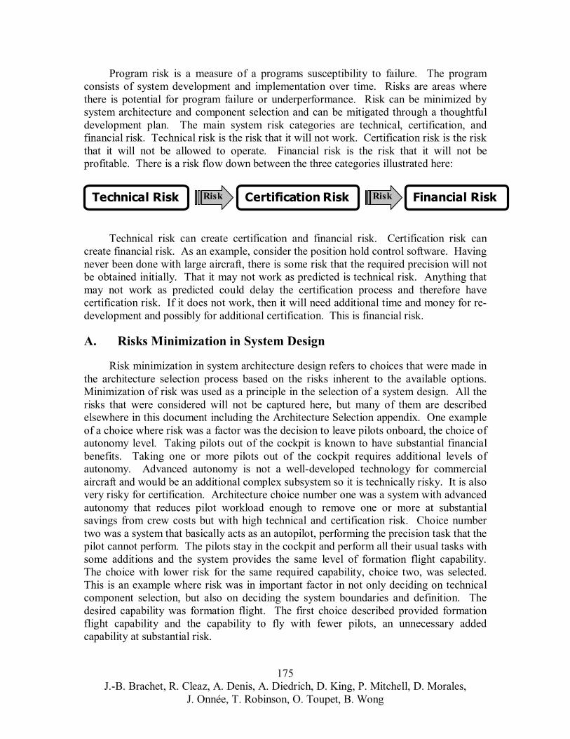
Program risk is a measure of a programs susceptibility to failure. The program consists of system development and implementation over time. Risks are areas where there is potential for program failure or underperformance. Risk can be minimized by system architecture and component selection and can be mitigated through a thoughtful development plan. The main system risk categories are technical, certification, and financial risk. Technical risk is the risk that it will not work. Certification risk is the risk that it will not be allowed to operate. Financial risk is the risk that it will not be profitable. There is a risk flow down between the three categories illustrated here:
Technical Risk Certification Risk Financial Risk Risk Risk
Technical risk can create certification and financial risk. Certification risk can create financial risk. As an example, consider the position hold control software. Having never been done with large aircraft, there is some risk that the required precision will not be obtained initially. That it may not work as predicted is technical risk. Anything that may not work as predicted could delay the certification process and therefore have certification risk. If it does not work, then it will need additional time and money for re-development and possibly for additional certification. This is financial risk.
A. Risks Minimization in System Design
Risk minimization in system architecture design refers to choices that were made in the architecture selection process based on the risks inherent to the available options. Minimization of risk was used as a principle in the selection of a system design. All the risks that were considered will not be captured here, but many of them are described elsewhere in this document including the Architecture Selection appendix. One example of a choice where risk was a factor was the decision to leave pilots onboard, the choice of autonomy level. Taking pilots out of the cockpit is known to have substantial financial benefits. Taking one or more pilots out of the cockpit requires additional levels of autonomy. Advanced autonomy is not a well-developed technology for commercial aircraft and would be an additional complex subsystem so it is technically risky. It is also very risky for certification. Architecture choice number one was a system with advanced autonomy that reduces pilot workload enough to remove one or more at substantial savings from crew costs but with high technical and certification risk. Choice number two was a system that basically acts as an autopilot, performing the precision task that the pilot cannot perform. The pilots stay in the cockpit and perform all their usual tasks with some additions and the system provides the same level of formation flight capability. The choice with lower risk for the same required capability, choice two, was selected. This is an example where risk was in important factor in not only deciding on technical component selection, but also on deciding the system boundaries and definition. The desired capability was formation flight. The first choice described provided formation flight capability and the capability to fly with fewer pilots, an unnecessary added capability at substantial risk.
175 J.-B. Brachet, R. Cleaz, A. Denis, A. Diedrich, D. King, P. Mitchell, D. Morales,
J. Onnée, T. Robinson, O. Toupet, B. Wong

Other risk minimization choices were made based on a near-term development effort. This was used when faced with two technologies at different stages of development, and both with potential for success. With no other factors, the choice that was further along in development was chosen to reduce risks. Differential GPS has been used successfully in formation flight and has been used in aircraft systems. This is less risky than an omni-directional laser that is a relatively new technology about which much less is known. If the system was being designed for a time further into the future the choice could have been to wait to see more results from omni-directional lasers and then make a choice instead of choosing differential GPS as was done.
B. Program Risks and Risk Mitigation
Remaining risk leftover after minimizing risk in system design becomes part of program risk. Program risk addresses the risk in developing the presented system. Risk is minimized with mitigation strategies. The most important risks, risk levels, and mitigation strategies are shown in the table below. Explanations of the risks follow.
Risk Risk Level
Mitigation Strategy
1 Vortices drift Low Parallel development of performance seeking control. Extensive vortex mapping early in the program
2 Required precision not realized
Low Alternate control strategies and sensing developed in parallel
3 Static or fatigue loading exceeded in vortex
Low Testing scheduled early in program
4 Vortices extremely unsteady
Low Early testing
5 Benefit overestimated Low Early testing 6 Development cost exceeded Low Very high ceiling, detailed cost study
recommended before commencing program
7 Not enough sales to cover development costs
Low Re-evaluate market before commencing. Sign-up customers and secure contracts before development. Sell to military.
8 Certification not approved Low Involve FAA early, consult before deciding to develop system.
9 Certification delayed Medium Certification, system test, and flight test plans submitted on-time and close consultation with FAA throughout.
10 Certification requires redesign
Low Consult with FAA on preliminary design when submitting certification plan. Close consultation throughout design process
Table 1: Program Risk Summary
176 J.-B. Brachet, R. Cleaz, A. Denis, A. Diedrich, D. King, P. Mitchell, D. Morales,
J. Onnée, T. Robinson, O. Toupet, B. Wong

1. Vortices drift
The position-hold type of control strategy proposed relies on accurate maps of vortex locations. The controller flies to a precise spot where the vortex should be located based on the flight conditions. It is possible that the vortex drifts, so that the trailing aircraft would be steady with respect the lead, but not with respect to the vortex, reducing time spent near the optimal location and thus the benefits.
The mitigation strategy is to go into proof-of-concept flight-testing very early in the program to find problems such as this one. Proof-of concept flight-testing would verify vortex properties and perform some initial system checks. The other mitigation strategy is a parallel development program for future upgrades that would include potentially better performing technologies, but that are riskier and at an earlier development stage. For the case of vortex drift, the parallel development of performance-seeking control could be accelerated. Performance seeking control should be able to follow drifting vortices.
2. Required precision not realized
If the controller cannot hold a precise enough position, then benefit will be reduced. Again, early testing will be used verify that the required precision can be held. If it
is not, analysis will hopefully be able to lead to a fix to the problem. Analysis may show that a technology in parallel development could solve the problem.
3. Static or fatigue loading exceeded in vortex
If the vortex is exceptionally turbulent, it is conceivable that the airplane could experience high loads, or fatigue loads that prevent long-term flights in the vortex.
Early testing will monitor structural loads. This requires that provisions for structural monitoring be made for the test airplanes. If excessive loads are found, the feasibility of introducing structural modifications should be investigated. Otherwise, the program should be ended.
4. Vortices extremely unsteady
This risk results from the lack of knowledge about vortex behavior. This basically covers the risk where tests show that vortex behavior would make any type of formation flight totally impossible.
Early tests would show this. It is highly unlikely.
5. Benefit overestimated
If the vortex is weaker than estimated, there may not be enough fuel savings to justify development.
Early tests should be able to show this. If this occurs, continuation of the program should be evaluated.
177 J.-B. Brachet, R. Cleaz, A. Denis, A. Diedrich, D. King, P. Mitchell, D. Morales,
J. Onnée, T. Robinson, O. Toupet, B. Wong
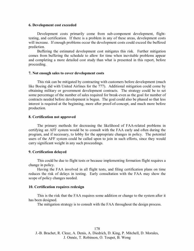
6. Development cost exceeded
Development costs primarily come from sub-component development, flight-testing, and certification. If there is a problem in any of these areas, development costs will increase. If enough problems occur the development costs could exceed the buffered prediction.
Buffering the estimated development cost mitigates this risk. Further mitigation comes from buffering the schedule to allow for time when inevitable problems appear and completing a more detailed cost study than what is presented in this report, before proceeding.
7. Not enough sales to cover development costs
This risk can be mitigated by contracting with customers before development (much like Boeing did with United Airlines for the 777). Additional mitigation could come by obtaining military or government development contracts. The strategy could be to set some percentage of the number of sales required for break-even as the goal for number of contracts needed before development is begun. The goal could also be phased so that less interest is required at the beginning, more after proof-of-concept, and much more before production.
8. Certification not approved
The primary methods for decreasing the likelihood of FAA-related problems in certifying an AFF system would be to consult with the FAA early and often during the program, and if necessary, to lobby for the appropriate changes in policy. The potential users of the AFF system could be called upon to join in such efforts, since they would carry significant weight in any such proceedings.
9. Certification delayed
This could be due to flight tests or because implementing formation flight requires a change in policy.
Having the FAA involved in all flight tests, and filing certification plans on time reduces the risk of delays in testing. Early consultation with the FAA may show the scope of policy changes needed.
10. Certification requires redesign
This is the risk that the FAA requires some addition or change to the system after it has been designed.
The mitigation strategy is to consult with the FAA throughout the design process.
178 J.-B. Brachet, R. Cleaz, A. Denis, A. Diedrich, D. King, P. Mitchell, D. Morales,
J. Onnée, T. Robinson, O. Toupet, B. Wong

179 J.-B. Brachet, R. Cleaz, A. Denis, A. Diedrich, D. King, P. Mitchell, D. Morales,
J. Onnée, T. Robinson, O. Toupet, B. Wong

XVII. Development Plan
180 J.-B. Brachet, R. Cleaz, A. Denis, A. Diedrich, D. King, P. Mitchell, D. Morales,
J. Onnée, T. Robinson, O. Toupet, B. Wong
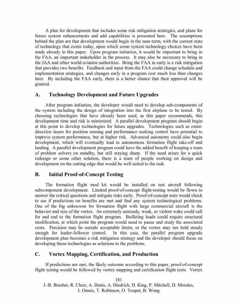
A plan for development that includes some risk mitigation strategies, and plans for future system enhancements and add capabilities is presented here. The assumptions behind the plan are that development would begin in the near-term, with the current state of technology that exists today, upon which some system technology choices have been made already in this paper. Upon program initiation, it would be important to bring in the FAA, an important stakeholder in the process. It may also be necessary to bring in the JAA and other world aviation authorities. Bring the FAA in early is a risk mitigation that provides two benefits. Feedback and input from the FAA could change schedule and implementation strategies, and changes early in a program cost much less than changes later. By including the FAA early, there is a better chance that their approval will be granted.
A. Technology Development and Future Upgrades
After program initiation, the developer would need to develop sub-components of the system including the design of integration into the first airplane to be tested. By choosing technologies that have already been used, as this paper recommends, this development time and risk is minimized. A parallel development program should begin at this point to develop technologies for future upgrades. Technologies such as omni-direction lasers for position sensing and performance seeking control have potential to improve system performance, but at higher risk. Advanced autonomy could also begin development, which will eventually lead to autonomous formation flight take-off and landing. A parallel development program could have the added benefit of keeping a team of problem solvers on standby, but still staying sharp. If the need arises for a quick redesign or some other solution, there is a team of people working on design and development on the cutting edge that would be well suited to the task.
B. Initial Proof-of-Concept Testing
The formation flight mod kit would be installed on test aircraft following subcomponent development. Limited proof-of-concept flight-testing would be flown to answer the critical questions and mitigate risks early. Proof-of-concept tests would check to see if predictions on benefits are met and find any system technological problems. One of the big unknowns for formation flight with large commercial aircraft is the behavior and size of the vortex. An extremely unsteady, weak, or violent wake could call for and end to the formation flight program. Buffeting loads could require structural modification, at which point the program would need to pause and study the associated costs. Precision may be outside acceptable limits, or the vortex may not hold steady enough for leader-follower control. In this case, the parallel program upgrade development plan becomes a risk mitigation strategy and the developer should focus on developing those technologies as solutions to the problems.
C. Vortex Mapping, Certification, and Production
If predictions are met, the likely outcome according to this paper, proof-of-concept flight testing would be followed by vortex mapping and certification flight tests. Vortex
181 J.-B. Brachet, R. Cleaz, A. Denis, A. Diedrich, D. King, P. Mitchell, D. Morales,
J. Onnée, T. Robinson, O. Toupet, B. Wong
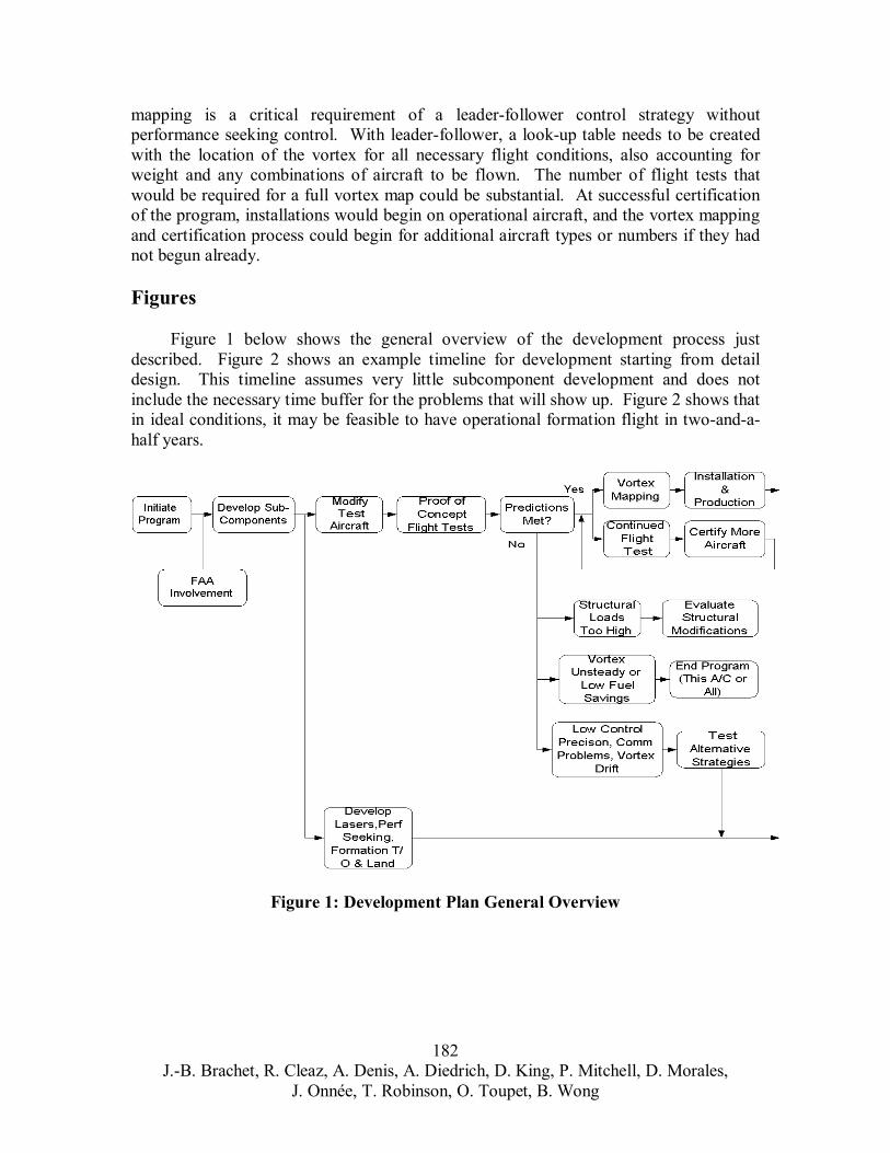
mapping is a critical requirement of a leader-follower control strategy without performance seeking control. With leader-follower, a look-up table needs to be created with the location of the vortex for all necessary flight conditions, also accounting for weight and any combinations of aircraft to be flown. The number of flight tests that would be required for a full vortex map could be substantial. At successful certification of the program, installations would begin on operational aircraft, and the vortex mapping and certification process could begin for additional aircraft types or numbers if they had not begun already.
Figures
Figure 1 below shows the general overview of the development process just described. Figure 2 shows an example timeline for development starting from detail design. This timeline assumes very little subcomponent development and does not include the necessary time buffer for the problems that will show up. Figure 2 shows that in ideal conditions, it may be feasible to have operational formation flight in two-and-a-half years.
Figure 1: Development Plan General Overview
182 J.-B. Brachet, R. Cleaz, A. Denis, A. Diedrich, D. King, P. Mitchell, D. Morales,
J. Onnée, T. Robinson, O. Toupet, B. Wong
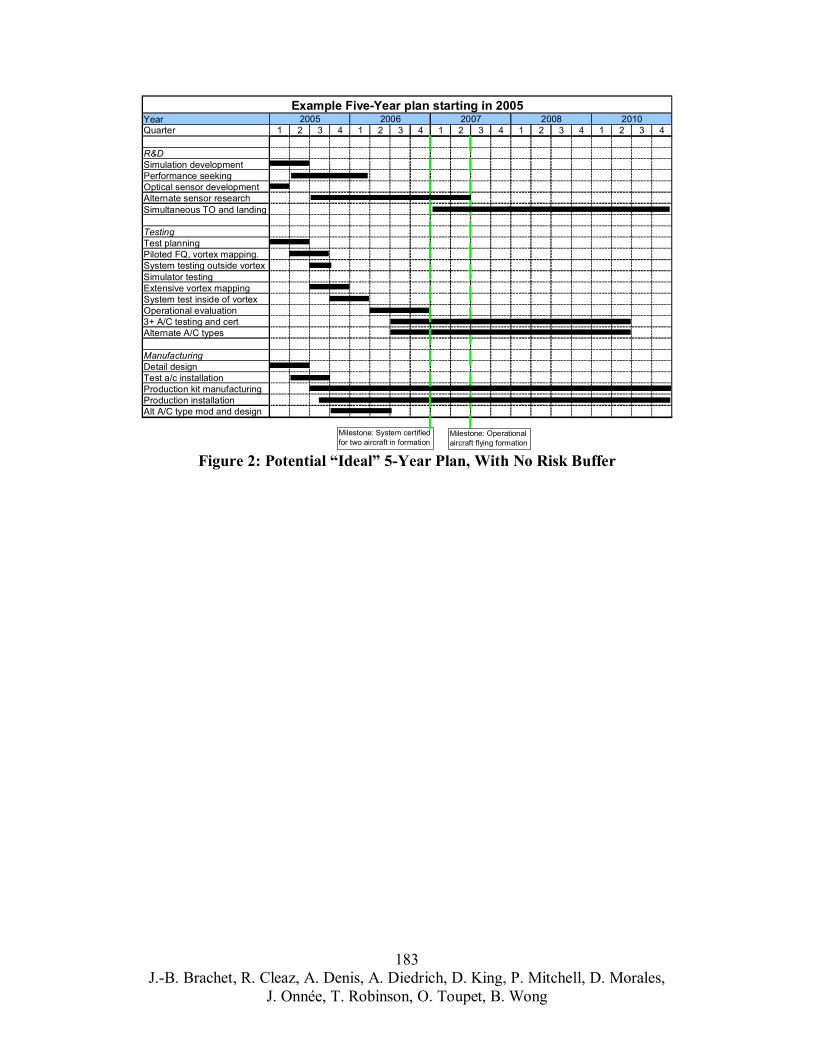
J.-B. Brachet, R. Cleaz, A. Denis, A. Diedrich, D. King, P. Mitchell, D. Morales, J. Onnée, T. Robinson, O. Toupet, B. Wong
183
YearQuarter 1 2 3 4 1 2 3 4 1 2 3 4 1 2 3 4 1 2 3 4
R&DSimulation developmentPerformance seekingOptical sensor developmentAlternate sensor researchSimultaneous TO and landing
TestingTest planningPiloted FQ, vortex mapping.System testing outside vortexSimulator testingExtensive vortex mapping System test inside of vortexOperational evaluation3+ A/C testing and certAlternate A/C types
ManufacturingDetail designTest a/c installationProduction kit manufacturingProduction installationAlt A/C type mod and design
Example Five-Year plan starting in 200520102005 2006 2007 2008
Milestone: System certified for two aircraft in formation
Milestone: Operationalaircraft flying formation
Figure 2: Potential “Ideal” 5-Year Plan, With No Risk Buffer

XVIII. Business Case
184 J.-B. Brachet, R. Cleaz, A. Denis, A. Diedrich, D. King, P. Mitchell, D. Morales,
J. Onnée, T. Robinson, O. Toupet, B. Wong
A. Business Case Outline
This document describes the business case for an Autonomous Formation Flight (AFF) system. It details the models used for performance estimation, the predicted cash expenditures in development and installation, and the potential benefits for each party involved in the development, installation, and operation of the system.
The primary parties that must be considered in the business case are a hypothetical developer of the AFF system and a cargo airline that may wish to equip its fleet with the system. For the case to close, both must be able to make a profit on the system. The definition of profit in this case will be a positive Net Present Value (NPV). By discounting future cash flows, the time value of money is represented.
For the developer case to close, an NPV calculation must yield a positive result within five years of the certification of the system. This five-year figure is set because it is the estimated time required to equip one airline’s fleet with the AFF system. Five years are required to allow each aircraft to be equipped during its C or D check. This will reduce the installation costs, since the aircraft is already out of service and partially dismantled.
For the cargo airline case to close, an NPV calculation must yield a positive result at the end of the time required to equip its fleet of aircraft with the AFF system. The calculations that follow will show that the cargo airline will probably not choose to outfit all of its aircraft with the AFF system, since it will only yield valuable returns for some aircraft. Accordingly, the business case becomes one in which the cargo airline must see a positive NPV at the end of the five-year equipping period for the aircraft it chooses to equip.
The business case has four main aspects. These aspects are listed and explained below.
1. Summary of performance benefits of formation flight. 2. The formation flight developer’s business case. 3. The cargo airline’s business case (with AFF). 4. The required/available market estimation.
The first section is a summary of probable performance benefits and the upper and lower expected variation of those benefits. These will be in the form of expected percent savings in fuel burn. Additionally, estimates are used for the amount of time required to form up and break down the formation at departure and destination. These estimates are made and justified in the ATC Procedures Appendix. The penalties for these times are taken into account. This results in a correlation between the potential benefits as a function of the type of aircraft, number of aircraft in the formation, departure and arrival configurations, and the range typically flown.
185 J.-B. Brachet, R. Cleaz, A. Denis, A. Diedrich, D. King, P. Mitchell, D. Morales,
J. Onnée, T. Robinson, O. Toupet, B. Wong
In the second section, an estimate of development and installation costs is produced for the hypothetical company developing the AFF system. These estimates will be used to produce figures for the required market penetration to consider the AFF system as a viable financial program.
The third section of the business case takes the benefit per aircraft information and the cost per installation information and returns an NPV calculation for an example cargo airline like FedEx or UPS.
The final section of the business case takes the information from the developer costs and the airline NPV calculation and determines how many airlines/aircraft are suitable for installation of an AFF system. This will then be compared with the market necessary to ensure profitability of the system. If the market can support the required amount of AFF installations, then the business case will be said to close for the developer.
In all of these sections, parametric studies are introduced to show how differences in the input parameters (recurring cost per kit, sales cost, fuel benefit) affect the market for the AFF system.
B. Performance Benefits of Formation Flight
Detailed information on the performance-related aspects of AFF is available in the Aerodynamic Performance Appendix. The information in this business case is restricted to a categorization of the probable results and the range over which these results could vary. The figure below shows the number of aircraft and the corresponding predicted benefits as a percentage of fuel savings. The various curves represent the best and worst cases as predicted by two theoretical models and observed in the NASA F/A 18 test flights. These are for the cruise condition only, and do not include any of the penalties associated with form-up, breakup, or rotation.
186 J.-B. Brachet, R. Cleaz, A. Denis, A. Diedrich, D. King, P. Mitchell, D. Morales,
J. Onnée, T. Robinson, O. Toupet, B. Wong
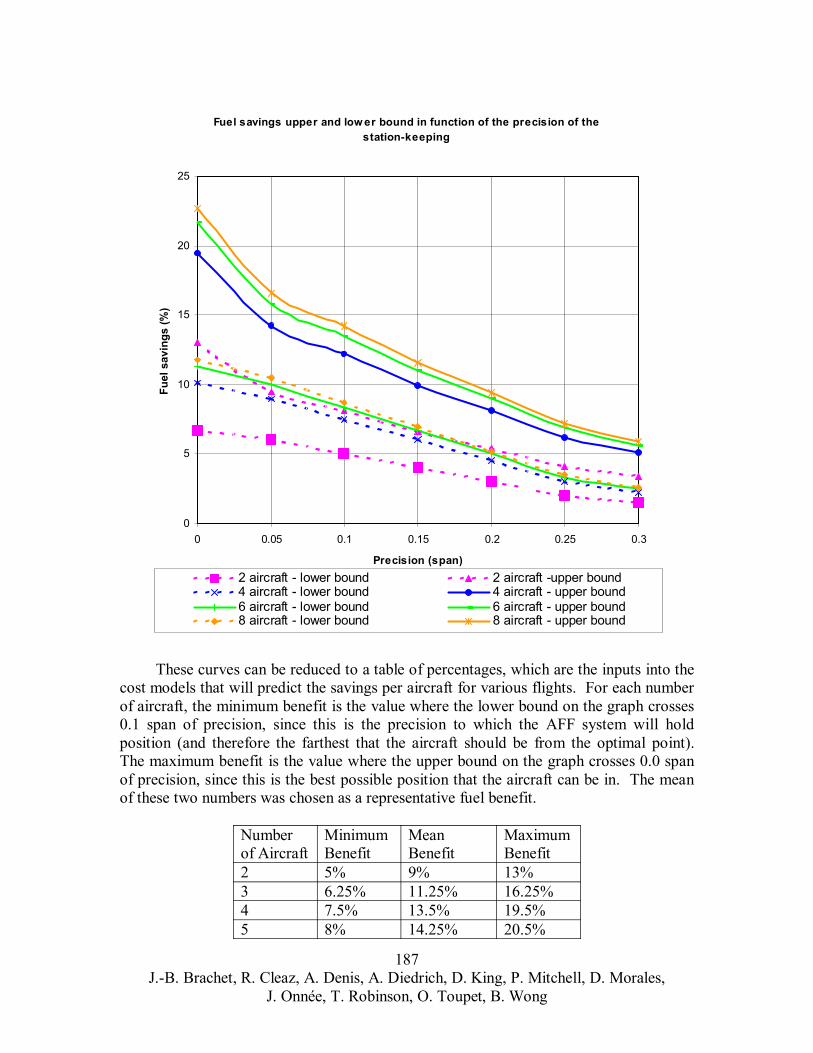
Fuel savings upper and low er bound in function of the precision of the station-keeping
Fuel
sav
ings
(%)
25
20
15
10
5
00 0.05 0.1 0.15 0.2 0.25 0.3
Precision (span) 2 aircraft - lower bound 2 aircraft -upper bound 4 aircraft - lower bound 4 aircraft - upper bound 6 aircraft - lower bound 6 aircraft - upper bound 8 aircraft - lower bound 8 aircraft - upper bound
These curves can be reduced to a table of percentages, which are the inputs into the cost models that will predict the savings per aircraft for various flights. For each number of aircraft, the minimum benefit is the value where the lower bound on the graph crosses 0.1 span of precision, since this is the precision to which the AFF system will hold position (and therefore the farthest that the aircraft should be from the optimal point). The maximum benefit is the value where the upper bound on the graph crosses 0.0 span of precision, since this is the best possible position that the aircraft can be in. The mean of these two numbers was chosen as a representative fuel benefit.
Number of Aircraft
Minimum Benefit
Mean Benefit
Maximum Benefit
2 5% 9% 13%3 6.25% 11.25% 16.25% 4 7.5% 13.5% 19.5% 5 8% 14.25% 20.5%
187 J.-B. Brachet, R. Cleaz, A. Denis, A. Diedrich, D. King, P. Mitchell, D. Morales,
J. Onnée, T. Robinson, O. Toupet, B. Wong
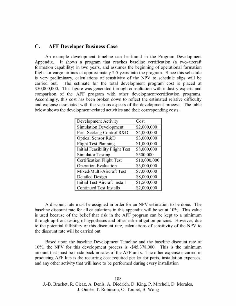
C. AFF Developer Business Case
An example development timeline can be found in the Program Development Appendix. It shows a program that reaches baseline certification (a two-aircraft formation capability) in two years, and assumes the beginning of operational formation flight for cargo airlines at approximately 2.5 years into the program. Since this schedule is very preliminary, calculations of sensitivity of the NPV to schedule slips will be carried out. The estimate for the total development program cost is placed at $50,000,000. This figure was generated through consultation with industry experts and comparison of the AFF program with other development/certification programs. Accordingly, this cost has been broken down to reflect the estimated relative difficulty and expense associated with the various aspects of the development process. The table below shows the development-related activities and their corresponding costs.
Development Activity Cost Simulation Development $2,000,000 Perf. Seeking Control R&D $4,000,000 Optical Sensor R&D $3,000,000 Flight Test Planning $1,000,000 Initial Feasibility Flight Test $8,000,000 Simulator Testing $500,000 Certification Flight Test $10,000,000 Operation Evaluation $3,000,000 Mixed/Multi-Aircraft Test $7,000,000 Detailed Design $8,000,000 Initial Test Aircraft Install $1,500,000 Continued Test Installs $2,000,000
A discount rate must be assigned in order for an NPV estimation to be done. The baseline discount rate for all calculations in this appendix will be set at 10%. This value is used because of the belief that risk in the AFF program can be kept to a minimum through up-front testing of hypotheses and other risk-mitigation policies. However, due to the potential fallibility of this discount rate, calculations of sensitivity of the NPV to the discount rate will be carried out.
Based upon the baseline Development Timeline and the baseline discount rate of 10%, the NPV for this development process is -$45,378,000. This is the minimum amount that must be made back in sales of the AFF units. The other expense incurred in producing AFF kits is the recurring cost required per kit for parts, installation expenses, and any other activity that will have to be performed during every installation
188 J.-B. Brachet, R. Cleaz, A. Denis, A. Diedrich, D. King, P. Mitchell, D. Morales,
J. Onnée, T. Robinson, O. Toupet, B. Wong

The recurring cost per AFF installation is estimated using two methods. The first is a comparison of per-installation costs for various other retrofit kits for commercial aircraft. This research showed that extensive non-structural modifications to aircraft could cost up to $500,000. Less extensive installations such as radios would usually cost less than $30,000. The AFF system is similar in complexity to the more complex systems.
In addition to the systems comparison, an element-by-element buildup of the AFF system was performed. The estimated sum of the major kit components (IMU, Carrier-Phase GPS, RF Transceivers, Formation Flight Manager), as well as duplicates for redundancy, is approximately $200,000. In order to account for the smaller components that are not modeled here and installation expenses, this figure is doubled to get the baseline recurring cost of $400,000 per unit.
The table of baseline conditions for the sale of AFF units is shown below:
Parameter Value NPV of Development Cost $45,378,000 Installation Start Time 2.5 years Installation Period 5 years Number of Aircraft to Outfit 127Sales Price for AFF Kit $1,000,000 Recurring Cost per Kit $400,000
This is a minimum sales case that results in an NPV just over zero. Many of these parameters are not precisely known. Therefore, sensitivity studies were carried out in order to determine how variations in each value affect the number of aircraft that must be outfitted to maintain an NPV greater than zero.
The first parameter variation is the installation start time. This is the number of years into the program at which money is first collected for the AFF kits. It is assumed to be collected for five years as a fleet of aircraft is outfitted. The graph below shows how program schedule slips affect the number of installations required to maintain a positive NPV.
189 J.-B. Brachet, R. Cleaz, A. Denis, A. Diedrich, D. King, P. Mitchell, D. Morales,
J. Onnée, T. Robinson, O. Toupet, B. Wong
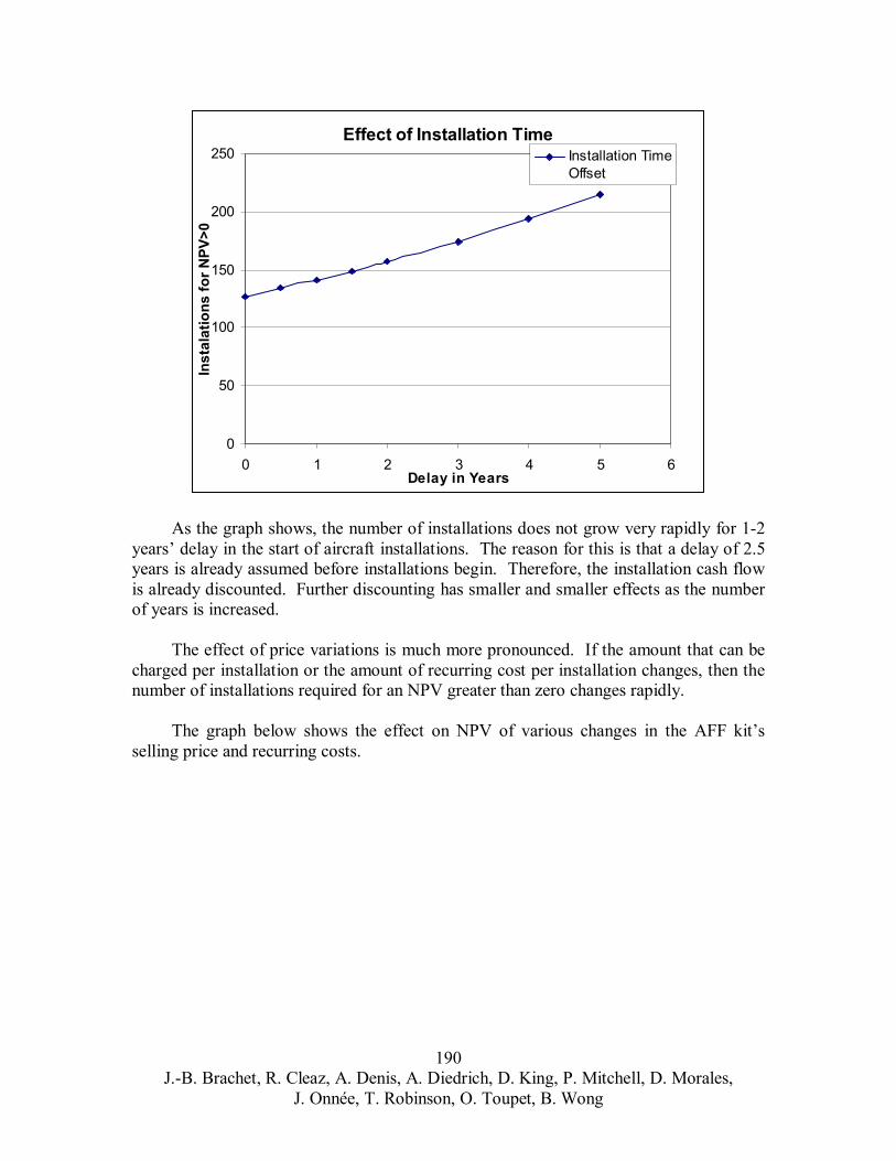
0
50
100
150
200
250
0 1 2 3 4 5 6
I l ion TiOff
Effect of Installation Time
Delay in Years
Inst
alat
ions
for N
PV>0
nstal at me set
As the graph shows, the number of installations does not grow very rapidly for 1-2 years’ delay in the start of aircraft installations. The reason for this is that a delay of 2.5 years is already assumed before installations begin. Therefore, the installation cash flow is already discounted. Further discounting has smaller and smaller effects as the number of years is increased.
The effect of price variations is much more pronounced. If the amount that can be charged per installation or the amount of recurring cost per installation changes, then the number of installations required for an NPV greater than zero changes rapidly.
The graph below shows the effect on NPV of various changes in the AFF kit’s selling price and recurring costs.
190 J.-B. Brachet, R. Cleaz, A. Denis, A. Diedrich, D. King, P. Mitchell, D. Morales,
J. Onnée, T. Robinson, O. Toupet, B. Wong
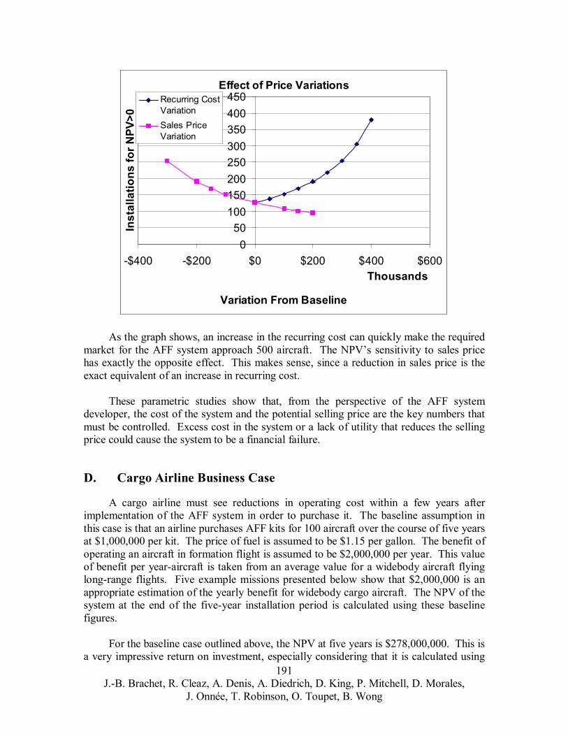
050
100150200250300350400450
$0 $200 $600
ii i
i i
Effect of Price Variations
-$400 -$200 $400 Thousands
Variation From Baseline
Inst
alla
tions
for N
PV>0
Recurr ng Cost Var at on Sales Price Var at on
As the graph shows, an increase in the recurring cost can quickly make the required market for the AFF system approach 500 aircraft. The NPV’s sensitivity to sales price has exactly the opposite effect. This makes sense, since a reduction in sales price is the exact equivalent of an increase in recurring cost.
These parametric studies show that, from the perspective of the AFF system developer, the cost of the system and the potential selling price are the key numbers that must be controlled. Excess cost in the system or a lack of utility that reduces the selling price could cause the system to be a financial failure.
D. Cargo Airline Business Case
A cargo airline must see reductions in operating cost within a few years after implementation of the AFF system in order to purchase it. The baseline assumption in this case is that an airline purchases AFF kits for 100 aircraft over the course of five years at $1,000,000 per kit. The price of fuel is assumed to be $1.15 per gallon. The benefit of operating an aircraft in formation flight is assumed to be $2,000,000 per year. This value of benefit per year-aircraft is taken from an average value for a widebody aircraft flying long-range flights. Five example missions presented below show that $2,000,000 is an appropriate estimation of the yearly benefit for widebody cargo aircraft. The NPV of the system at the end of the five-year installation period is calculated using these baseline figures.
For the baseline case outlined above, the NPV at five years is $278,000,000. This is a very impressive return on investment, especially considering that it is calculated using
191 J.-B. Brachet, R. Cleaz, A. Denis, A. Diedrich, D. King, P. Mitchell, D. Morales,
J. Onnée, T. Robinson, O. Toupet, B. Wong
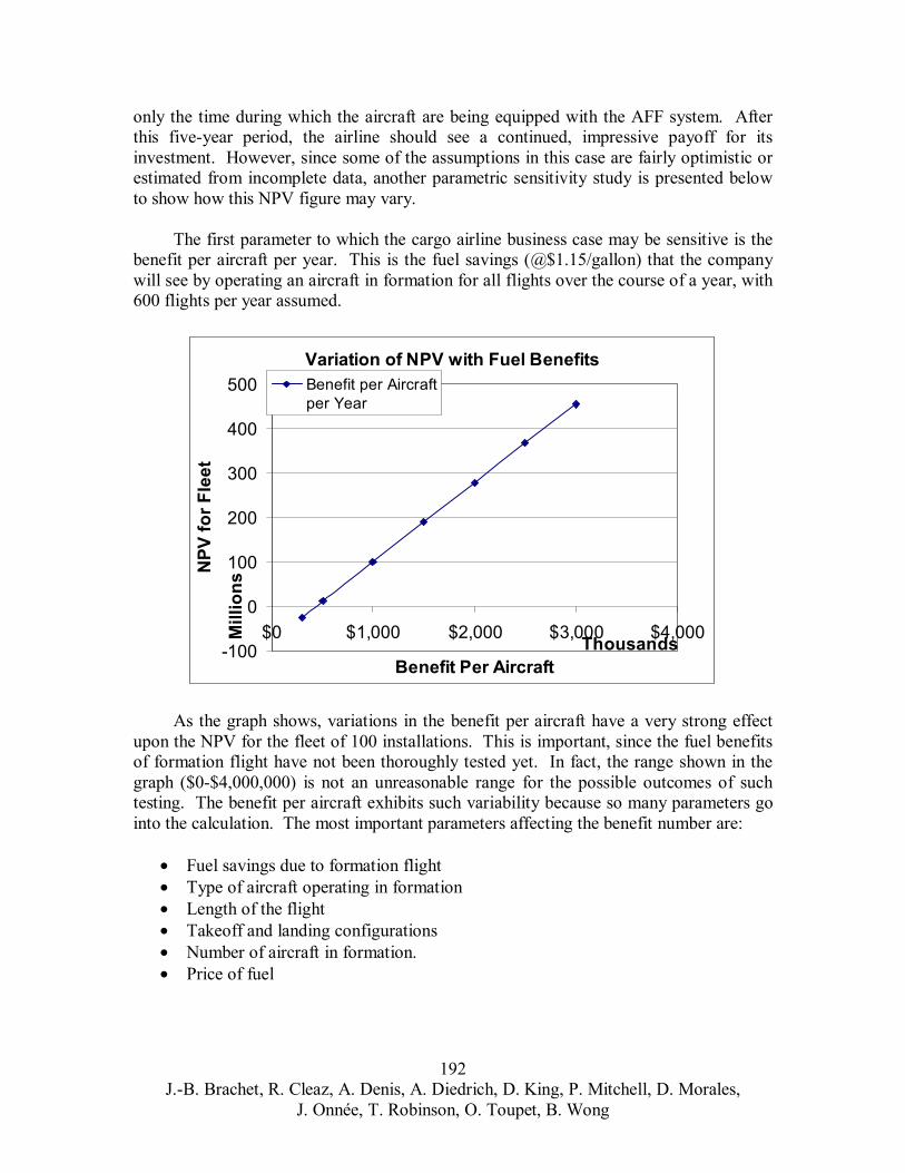
only the time during which the aircraft are being equipped with the AFF system. After this five-year period, the airline should see a continued, impressive payoff for its investment. However, since some of the assumptions in this case are fairly optimistic or estimated from incomplete data, another parametric sensitivity study is presented below to show how this NPV figure may vary.
The first parameter to which the cargo airline business case may be sensitive is the benefit per aircraft per year. This is the fuel savings (@$1.15/gallon) that the company will see by operating an aircraft in formation for all flights over the course of a year, with 600 flights per year assumed.
0
100
200
300
400
500
$0
iVariation of NPV with Fuel Benefits
-100 $1,000 $2,000 $3,000 $4,000 M
illio
ns
Thousands Benefit Per Aircraft
NPV
for F
leet
Benefit per A rcraft per Year
As the graph shows, variations in the benefit per aircraft have a very strong effect upon the NPV for the fleet of 100 installations. This is important, since the fuel benefits of formation flight have not been thoroughly tested yet. In fact, the range shown in the graph ($0-$4,000,000) is not an unreasonable range for the possible outcomes of such testing. The benefit per aircraft exhibits such variability because so many parameters go into the calculation. The most important parameters affecting the benefit number are:
• Fuel savings due to formation flight • Type of aircraft operating in formation • Length of the flight • Takeoff and landing configurations • Number of aircraft in formation. • Price of fuel
192 J.-B. Brachet, R. Cleaz, A. Denis, A. Diedrich, D. King, P. Mitchell, D. Morales,
J. Onnée, T. Robinson, O. Toupet, B. Wong

The second sensitivity study looks at what sales price the cargo airline can afford to pay for the AFF system, depending upon how much benefit per aircraft the airline sees. The graph below shows the NPV for various sales prices and benefit values.
Vi
$0
$20
$40
$60
$80
$100
NPV
i
i
i
ariation in NPV with Benefit per Aircraft and Sales Pr ce
-$40
-$20 -$1,000 -$500 $0 $500 $1,000 $1,500 $2,000
Mill
ions
Thousands
Sales Price Variation from Baseline
Benef t = $1,000,000
Benef t = $500,000
Benef t = $300,000
As the graph shows, for the baseline sales price of $1,000,000, the benefit must be approximately $450,000 per aircraft-year for the AFF system to look like a good buy to the airline. However, if the sales price is dropped by approximately $300,000 to a value of $700,000 per installation, then even a benefit of $300,000 per aircraft-year results in an NPV of zero. This also allows more aircraft to be outfitted with the AFF system, so the decreased sales price can be offset for the developer by an increased number of sales.
More analysis is needed in order to fully evaluate the utility of the AFF system to an airline. The benefit per aircraft must be shown as a function of the size of the aircraft and the percentage of fuel saved. Several specific cases from UPS’s daily schedule were calculated. These are listed below. The benefits listed are all per aircraft per year for 600 flights a year and $1.15 per gallon of jet fuel.
1) A 747-100 flying from Anchorage, Alaska to Seoul, S. Korea (3290 nm) in formation with one other aircraft for 100% of its flight: a. Lowest Estimated Benefit: $819,480 b. Mean Estimated Benefit: $1,543,000 c. Highest Estimated Benefit: $2,266,500
2) A 747-100 flying from Anchorage, Alaska to Hong Kong (4406 nm) in formation with one other aircraft for 100% of its flight:
193 J.-B. Brachet, R. Cleaz, A. Denis, A. Diedrich, D. King, P. Mitchell, D. Morales,
J. Onnée, T. Robinson, O. Toupet, B. Wong
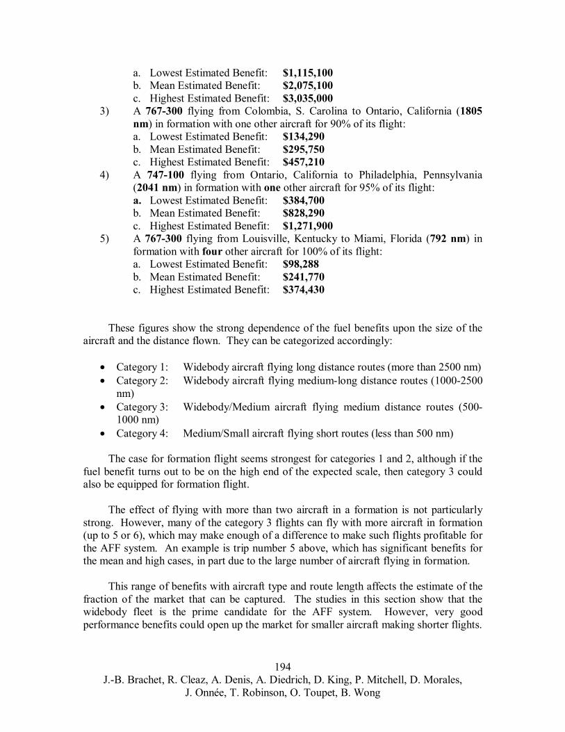
a. Lowest Estimated Benefit: $1,115,100 b. Mean Estimated Benefit: $2,075,100 c. Highest Estimated Benefit: $3,035,000
3) A 767-300 flying from Colombia, S. Carolina to Ontario, California (1805nm) in formation with one other aircraft for 90% of its flight: a. Lowest Estimated Benefit: $134,290 b. Mean Estimated Benefit: $295,750 c. Highest Estimated Benefit: $457,210
4) A 747-100 flying from Ontario, California to Philadelphia, Pennsylvania (2041 nm) in formation with one other aircraft for 95% of its flight: a. Lowest Estimated Benefit: $384,700 b. Mean Estimated Benefit: $828,290 c. Highest Estimated Benefit: $1,271,900
5) A 767-300 flying from Louisville, Kentucky to Miami, Florida (792 nm) in formation with four other aircraft for 100% of its flight: a. Lowest Estimated Benefit: $98,288 b. Mean Estimated Benefit: $241,770 c. Highest Estimated Benefit: $374,430
These figures show the strong dependence of the fuel benefits upon the size of the aircraft and the distance flown. They can be categorized accordingly:
• Category 1: Widebody aircraft flying long distance routes (more than 2500 nm) • Category 2: Widebody aircraft flying medium-long distance routes (1000-2500
nm) • Category 3: Widebody/Medium aircraft flying medium distance routes (500-
1000 nm) • Category 4: Medium/Small aircraft flying short routes (less than 500 nm)
The case for formation flight seems strongest for categories 1 and 2, although if the fuel benefit turns out to be on the high end of the expected scale, then category 3 could also be equipped for formation flight.
The effect of flying with more than two aircraft in a formation is not particularly strong. However, many of the category 3 flights can fly with more aircraft in formation (up to 5 or 6), which may make enough of a difference to make such flights profitable for the AFF system. An example is trip number 5 above, which has significant benefits for the mean and high cases, in part due to the large number of aircraft flying in formation.
This range of benefits with aircraft type and route length affects the estimate of the fraction of the market that can be captured. The studies in this section show that the widebody fleet is the prime candidate for the AFF system. However, very good performance benefits could open up the market for smaller aircraft making shorter flights.
194 J.-B. Brachet, R. Cleaz, A. Denis, A. Diedrich, D. King, P. Mitchell, D. Morales,
J. Onnée, T. Robinson, O. Toupet, B. Wong
E. Market Estimation
As the previous sections have shown, the number of aircraft that a developer of an AFF system must outfit varies widely depending upon sales price and recurring cost. The cargo airline’s demand for the system varies just as widely depending upon the sales price and the performance of the system. All three of these parameters (sales price, recurring cost, and performance) must be known before accurate market estimation can be done. However, as with the other sections of this business case, some knowledge can be gained through parametric studies of the relationships between these numbers.
For instance, in the case where the all of the estimates about performance and costs are accurate, then the developer of the AFF system should find ample market space for the system, even if the price is increased to $2,000,000 per kit. As the graph showing variations in sales price and benefit shows, for $2,000,000 per kit (shown as a $1,000,000 variation from baseline), the NPV is +$20,000,000 per 100 aircraft outfitted at $1,000,000 yearly benefit per aircraft. The listing of example missions shows that $1,000,000 per aircraft is easy to achieve with wide-body, long haul aircraft.
If the fuel benefits of formation flight are as high as the highest estimated performance, then the cargo airline could actually outfit many medium-range aircraft with the system. The last example flight above (from Louisville to Miami) shows benefits of $374,430 at the highest benefit level. For this level, if the developer drops sales price to around $750,000, then all medium- and long-range cargo aircraft are candidates, the NPV for the cargo airline is positive, and the required sales for the developer are around 220 aircraft. This is not an unreasonable sales number, as it represents about half of either FedEx or UPS’s fleet of jet aircraft.
F. Calculation Methodology
The models in this business case rely heavily on the first graph in this appendix, a plot of fuel benefit as a function of precision in station keeping. This plot was produced by Amandine Denis. The rest of the models are MATLAB functions that translate these benefits and the aircraft performance figures into dollars and cents. The workings of some of the key functions are outlined below.
The first function sets up the characteristics of a particular formation flight, namely the number of aircraft in formation at each of 20 points along the cruise path, the takeoff and landing conditions (in formation, on parallel runways, not in formation, etc), the type of aircraft, the distance flown, and the estimated fuel benefit due to formation flight (the lowest, mean, or highest case).
The second function takes in this data and calculates estimated fuel burn during a normal flight and during a formation flight. This is done with performance data from BADA. The difference between the two fuel burns is a savings in pounds of fuel per
195 J.-B. Brachet, R. Cleaz, A. Denis, A. Diedrich, D. King, P. Mitchell, D. Morales,
J. Onnée, T. Robinson, O. Toupet, B. Wong
flight. This is translated into gallons and then dollars. A year’s worth of flights is then summed to produce the benefit per aircraft per year.
The developer business case uses the development timeline created by Dan King. Each activity is first assigned a value in dollars as shown in the first section. It is also assigned a time during the development, as in the development timeline. The discount rate of 10% per year is then applied to this development process, and the resulting NPV for development is calculated.
The return for the developer is calculated using a sales price per installation, recurring costs per installation, number of aircraft to be modified, number of years over which to modify the aircraft, and a time offset in years which represents the time after the start of the program at which installations begin. From these numbers, an NPV for the sales can be calculated. The NPV for the development can then be subtracted from the NPV for the sales to calculate the overall NPV.
The airline business case uses the same AFF kit sales data as the developer business case. The monetary benefit per aircraft must then be added. The benefit numbers are phased in year by year, just as the aircraft with the system would be phased in. For example, during the first year, 20% of the aircraft have the AFF system installed, and each one has it installed for an average of 50% of the year, so the benefits received are only 10% of the total for an entire fleet. This number grows until the fifth year, during which 100% of the fleet has the AFF system, but 20% received it that year, so benefits are 90% of the full level. These benefits are then summed (after time-discounting), and the NPV for the airline’s return can be calculated and summed with their costs of installation.
All of these functions were run for multiple inputs to derive the parametric studies presented in each of the previous sections of this business case.
G. Conclusions
The business case for autonomous formation flight is quite promising for long-range air cargo. However, no absolute claims can be made with a parametric study, unless some of the parameters can be fixed. The study only provides hypothetical conclusions. However, it does show which parameters are crucial to the profitability of the AFF system to the developer and the airline (fuel benefits being the most important), and which ones are not quite as important (slippage in installation scheduling).
Once testing does begin on a system such as the AFF, however, a parametric business case allows the developer to quickly and easily determine whether the system is really viable, what markets to go after, what prices to set, and how much market penetration is needed at a particular price point. Such knowledge can serve as a very important risk estimation and mitigation tool, allowing stakeholders to know how likely it is that the program can succeed with a minimum of information about the future.
196 J.-B. Brachet, R. Cleaz, A. Denis, A. Diedrich, D. King, P. Mitchell, D. Morales,
J. Onnée, T. Robinson, O. Toupet, B. Wong