Visual Coverage Control for Teams of Quadcoptersvia Control Barrier Functions

Riku Funada1, Marıa Santos2, Junya Yamauchi1, Takeshi Hatanaka3, Masayuki Fujita1, and Magnus Egerstedt2

Abstract— This paper presents a coverage control strategyfor teams of quadcopters that ensures that no area is leftunsurveyed in between the fields of view of the visual sensorsmounted on the quadcopters. We present a locational costthat quantifies the team’s coverage performance according tothe sensors’ performance function. Moreover, the cost functionpenalizes overlaps between the fields of view of the differentsensors, with the objective of increasing the area covered by theteam. A distributed control law is derived for the quadcoptersso that they adjust their position and zoom according to thedirection of ascent of the cost. Control barrier functions areimplemented to ensure that, while executing the gradient ascentcontrol law, no holes appear in between the fields of viewof neighboring robots. The performance of the algorithm isevaluated in simulated experiments.

I. INTRODUCTION

An increasing number of visual sensors have been intro-duced in urban areas and natural environments [1] with thegoal of collecting information about events such as naturalphenomena [2], security concerns [3] and urban traffic [4].Although, for some applications, a stationary network ofvisual sensors may be sufficient to obtain the necessaryinformation [5], [6], [7], [8], aerial robotic swarms representan adaptable solution for scenarios where the domain to bemonitored or the surveillance requirements may vary [9].

Coordinating a group of aerial robots to visually monitorareas of interest can be considered in the context of thecoverage problem [10], [11], [12]. Coverage control dealswith how to distribute a collection of mobile sensors in adomain such that the features of interest are appropriatelymonitored by the team. The quality of the surveillanceover the objective area is often quantified according to theperformance function of the sensors [13], [14], [15]. Formulti-camera systems, the problem of visual coverage hasbeen explored both for stationary camera networks [16],[17] and for cameras on teams of quadcopters [18], [19].In these scenarios, aspects such as lens distortion [17] or

*This work was supported by JSPS KAKENHI Grant Number 16J07893and by ARL through grant DCIST CRA W911NF-17-2-0181.

1R. Funada, J. Yamauchi and M. Fujita are with Departmentof Systems and Control Engineering, Tokyo Institute of Technol-ogy, Tokyo 152-8550, Japan funada@fl.ctrl.titech.ac.jp{yamauchi,fujita}@sc.e.titech.ac.jp

2M. Santos and M. Egerstedt are with the School of Electrical andComputer Engineering, Georgia Institute of Technology, Atlanta, GA 30332,USA {maria.santos,magnus}@gatech.edu

3T. Hatanaka is with Electronic and Information Engineering, Grad-uate School of Engineering, Osaka University, Osaka, 565-0871, Japanhatanaka@eei.eng.osaka-u.ac.jp

camera resolution [18] are usually taken into account whenquantifying the coverage performance of the system.

In this paper, we present a visual coverage algorithmfor teams of quadcopters equipped with downward facingcameras. Although the scenario is similar to [18], [19], wepropose a new locational cost that simultaneously servestwo purposes: (a) quantifying the performance of all thecameras, taking into account their lens distortion as in [17];and (b) reducing the overlap between fields of view ofthe quadcopters, to expand the surveyed area as much aspossible. However, increasing the covered area may result inthe appearance of coverage holes, that is, unsurveyed areasin between contiguous agents that significantly degrade thecoverage performance [15], [20], [21], [22]. To prevent thisunfavorable situation, the proposed algorithm incorporatescontrol barrier functions [23] among agents whose fields ofview form triangulations to ensure that no holes appear inbetween covered areas.

The remainder of the paper is organized as follows: InSection II, we formalize the problem statement. A newlocational cost that encodes the coverage performance of theteam and minimizes overlaps between the quadcopters’ fieldsof view is introduced in Section III. A distributed controlstrategy which allows the team to achieve a critical point ofthe cost by performing an ascent flow is derived in SectionIII-A. Section IV introduces a control barrier function thatensures that the fields of view of neighboring agents inthe team stay connected. The performance of the proposedmethod is evaluated in simulation in Section V. Section VIconcludes the paper.

II. PROBLEM STATEMENTConsider the scenario illustrated in Fig. 1, where n quad-

copters, indexed by N = {1, · · · , n}, are distributed over the3D Euclidean space with the objective of covering a planarregion, hereafter referred to as the mission space and denotedas Q. The mission space is a closed and bounded convexset within a planar environment, E . A density function,φ : Q → R, can be used to encode the importance ofeach point within the mission space such that, the higherthe importance, the higher the value of the density function.

Without loss of generality, the world coordinate frame,Σw, is chosen to be right-handed, with the XYw-planecoplanar to E . If we denote the standard basis of Σw as{ex, ey, ez}, then the environment is

E = {q ∈ R3 | eTz q = 0},

and the quadcopters are naturally restricted to move in thehalf space {q ∈ R3 | eTz q > 0}.

In order to monitor the environment, each quadcopter isequipped with a downward facing visual sensor. Let Σi be theframe of reference of Quadcopter i, i ∈ N , located at pi =[xi, yi, zi]

T with respect to Σw and with its standard basisbeing parallel to the basis of the world frame while hovering,i.e., Σi not rotated with respect to Σw. We assume that thevisual sensor is mounted on the quadcopter using a gimbalsuch that its image plane is always parallel to the XYi-planeand Zi is aligned with the optical axis. If we express theimage projection according to a perspective projection model[24], then the origin of Σi is located at a distance equal tothe focal length, λi, above the image plane. In this paper,the image plane of all agents is assumed to be circular withradius r.

Each quadcopter can therefore monitor the portion of themission space Q in its field of view,

Fi =

{q ∈ E

∣∣∣∣ ‖q − [xi, yi, 0]T ‖ ≤ r ziλi

},

which depends on the position of the quadcopter, pi, and onthe zoom level of its visual sensor, determined by the focallength, λi.

The objective of this paper is to achieve a spatial allocationof the team and focal length for each agent such that thecombination of all the fields of view {F1, . . . ,Fn} resultsin an optimal coverage of the mission space, Q. Let pi =[pTi , λi]

T be the state of Quadcopter i. We assume that themovement of the quadcopter can be controlled according tosingle integrator dynamics,

pi = ui, (1)

which can be converted to reflect the quadcopter’s dynamics,e.g. as in [25]. With this consideration, the state of the agentscan evolve to satisfy three different aspects of the coverageobjective: (a) the areas of higher importance in the missionspace need to be monitored closely by the quadcopters, (b)the area covered by the quadcopters should expand as muchas possible over the mission space, while ensuring that (c)no space in between fields of view of contiguous robots isleft unsurveyed. We encode requirements (a) and (b) througha locational cost to be optimized by the agents, while (c) isenforced through control barrier functions.

III. COVERAGE CONTROLA natural way of characterizing the coverage performance

of a multi-robot team over a domain of interest, Q, is todefine a cost function that quantifies the team’s collectiveperformance as a function of the quadcopters’ states. Thequality of surveillance at a point q ∈ Q in the field of viewFi can be quantified using the model in [17],

f(pi, q) = fpers(pi, q)fres(pi, q), (2)

with fpers(pi, q) characterizing the perspective quality,

fpers(pi, q) :=

√λ2i + r2√

λ2i + r2 − λi

(zi

‖q − pi‖− λi√

λ2i + r2

),

Image

Plane

Fig. 1. Proposed scenario. The teams of quadcopters monitor the missionspace Q. Agent i’s field of view Fi depends on Agent i’s position, pi, andfocal length, λi. The crosshatched area among the quadcopters’ field ofviews represents a hole. By using control barrier functions, we will preventthis unsurveyed area from emerging while maximizing the coverage cost.

and fres(pi, q) the loss of resolution,

fres(pi, q) :=

(λi√λ2i + r2

)κexp

(− (‖q − pi‖ −R)2

2σ2

).

Analogously to [17], the parameters κ, σ > 0 model thespatial resolution variability of the sensor and R > 0represents the desired range for the vision sensor. If a pointis not in the field of view of Quadcopter i, then

f(pi, q) = 0, q /∈ Fi.

Having defined the sensing performance function, thequality of the coverage performed by the quadcopter teamcan be characterized through the cost,

HC(p) =

∫Q

maxi∈N

f(pi, q)φ(q)dq, (3)

with a higher value of the cost corresponding to a bettercoverage of the domain. Here p = [pT1 , . . . ,p

Tn ]T is the

combined state of all the robots and the subscript C refers tothe fact that this cost quantifies the coverage quality. Equiv-alently, if we define the region of dominance of Quadcopteri according to the conic Voronoi diagram [17],

Vi(p) = {q ∈ Q ∩ Fi | f(pi, q) ≥ f(pj , q), j ∈ N}, (4)

the cost in (3) becomes,

HC(p) =∑i∈N

∫Vi(p)

f(pi, q)φ(q)dq. (5)

However, characterizing the coverage performance as in(5) implies that, at a point q ∈ Q where several fields of viewoverlap, only the state of the quadcopter with the best sensingperformance at q contributes to the coverage objective. Thiscan be detrimental for the team since those quadcopters witha suboptimal coverage of q could potentially cover alternativeareas of the mission space. Let us denote the area coveredby Quadcopter i where another quadcopter in the team hasa superior sensing performance as

Vi(p) = {q ∈ Q ∩ Fi | f(pi, q) < f(pj , q), j ∈ N}.

Then, the performance loss caused by the area overlap canbe quantified as

HO(p) =∑i∈N

∫Vi(p)

f(pi, q)φ(q)dq. (6)

We are interested in minimizing the cost in (6) since itcharacterizes the loss of performance caused by the overlapsamong the fields of view. Therefore, we can encode theoverall objective combining (6) with (5) as follows,

H(p) = HC(p)−HO(p), (7)

with a higher value of H corresponding to a better perfor-mance of the team under the specified objectives.

A. Gradient Ascent

Having defined a locational cost that characterizes theperformance of the team, a natural way to maximize it isto make the quadcopters follow a direction of ascent, that is,

pi =∂H(p)

∂pi

T

, i ∈ N .

In order to compute the gradient of (7), let us first considerthe gradient of HC by applying Leibniz integral rule [26],

∂HC(p)

∂pi=

∫Vi

∂f(pi, q)

∂piφ(q)dq (8)

+

∫∂Vi

f(pi, q)φ(q)nTij(q)∂q

∂pidq (9)

+∑j∈Ni

∫∂Vij

f(pj , q)φ(q)nTji(q)∂q

∂pidq, (10)

where Ni are the neighbors of i with respect to the partitionin (4),

Ni = {j ∈ N | f(pi, q) = f(pj , q), q ∈ Q}, (11)

and ∂Vi and ∂Vij denote the whole boundary of Vi and thoseparts of the boundary shared with Quadcopter j, respectively.We have dropped the dependency of Vi and its boundarieson p for notational convenience.

The term in (9) corresponds to a line integral whosedomain of integration, ∂Vi, can be composed of

1) boundaries resulting from the overlap of the fields ofview of Quadcopter i and other quadcopter’s, ∂Vij ;

2) segments along the boundary of the mission space,where Vi ∩ ∂Q; and

3) arcs of circumference where Fi intersects with theinterior of the mission space without overlapping withany other agent.

In 1), the terms integrated over ∂Vij cancel the correspondingterm in (10), given that

f(pi, q) = f(pj , q), q ∈ ∂Vij , (12)

and the normals are opposite to each other, nij(q) =−nji(q). For case 2), the term ∂q/∂pi in the integrand iszero, and thus vanishes along those segments. Finally, thesensing performance f(pi, q) = 0 in the boundary of thefield of view, Fi, and, thus, the integrals corresponding to

case 3) also become zero. Therefore, the gradient of HC(pi)is

∂HC(p)

∂pi=

∫Vi

∂f(pi, q)

∂piφ(q)dq.

The expression for the derivative of the sensing perfor-mance function with respect to the state of Quadcopter i,∂f(pi, q)/∂pi, is included in the Appendix.

A similar analysis follows for the gradient of HO,

∂HO(p)

∂pi=

∫Vi

∂f(pi, q)

∂piφ(q)dq.

Therefore, the gradient of H,

∂H(p)

∂pi=

∫Vi

∂f(pi, q)

∂piφ(q)dq −

∫Vi

∂f(pi, q)

∂piφ(q)dq.

(13)Letting Quadcopter i follow a direction of ascent estab-

lishes the following coverage theorem.Theorem 1: Let Quadcopter i, with state pi = [pTi , λi]

T ,evolve according to the control law pi = u, with

u =

∫Vi

∂f(pi, q)

∂pi

T

φ(q)dq −∫Vi

∂f(pi, q)

∂pi

T

φ(q)dq, (14)

then, as t → ∞, the quadcopter team will converge to acritical point of the locational cost in (7).

Proof: Let us consider the candidate function

V (p) = U −H(p) > 0, (15)

with U =∫Q φ(q)dq a strict upper bound of the locational

cost, H(p), given that f(pi, q) ∈ [0, 1],∀i ∈ N . Then, thetotal derivative of (15),

dV

dt= −

∑i∈N

∂H∂pi

pi = −

∥∥∥∥∥∂H∂p T∥∥∥∥∥

2

≤ 0. (16)

For (16) to be zero, we need ∂H/∂p = 0, which correspondsto pi = 0. By LaSalle’s invariance principle, the team willconverge to the largest invariant set contained in the set thatsatisfies ∂H/∂p = 0, i.e. the critical points of the cost (7).

IV. CONTROL BARRIER FUNCTIONS

Although the control input (14) allows the quadcopterteam to fulfill the two objectives stated in Section II, namely,monitoring important areas with the appropriate resolutionand expanding the covered area as much as possible; weneed to enforce that no area is left unsurveyed in the middleof monitored areas, as illustrated in Fig. 1. If such an areaappears, the fields of view surrounding it will prevent anyother member of the team from covering it. Thus, the chanceof monitoring a hole once it arises is very small.

In order to analyze the existence of coverage holes, weneed to characterize the neighborhood of each agent. LetGF (p) denote the graph given by the conic Voronoi partition,with neighborhoods given by (11), and GP(p) the powerdiagram [27] characterized by the weighted distance,

dP(pi, q) = ‖[qx, qy]T − [xi, yi]T ‖2 −∆2

i ,

where ∆i = rzi/λi is the radius of Fi. The graph G(p) =GF ∩ GP preserves the edges of the power diagram onlybetween those neighbors whose fields of view overlap.Analogously to other works in sensor networks which usetriangulations [28], [29], we concern ourselves with triangu-lar subgraphs [30] of the graph G(p).

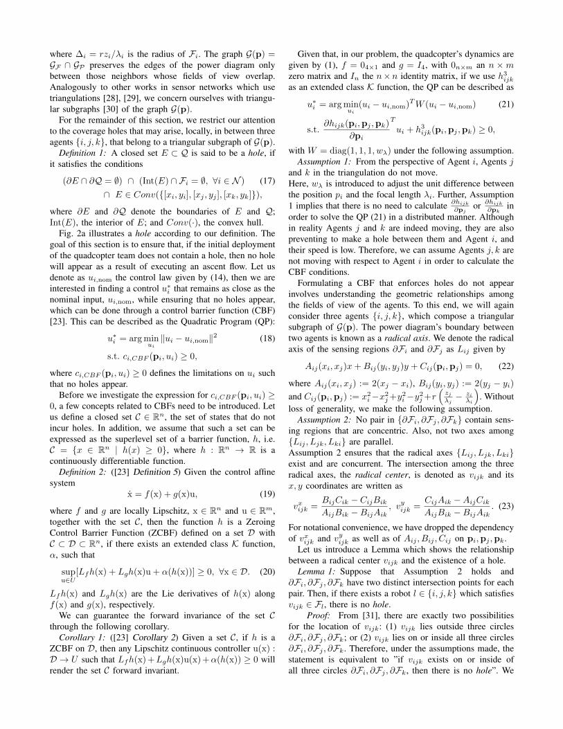
For the remainder of this section, we restrict our attentionto the coverage holes that may arise, locally, in between threeagents {i, j, k}, that belong to a triangular subgraph of G(p).

Definition 1: A closed set E ⊂ Q is said to be a hole, ifit satisfies the conditions

(∂E ∩ ∂Q = ∅) ∩ (Int(E) ∩ Fi = ∅, ∀i ∈ N ) (17)∩ E ∈ Conv({[xi, yi], [xj , yj ], [xk, yk]}),

where ∂E and ∂Q denote the boundaries of E and Q;Int(E), the interior of E; and Conv(·), the convex hull.

Fig. 2a illustrates a hole according to our definition. Thegoal of this section is to ensure that, if the initial deploymentof the quadcopter team does not contain a hole, then no holewill appear as a result of executing an ascent flow. Let usdenote as ui,nom the control law given by (14), then we areinterested in finding a control u∗i that remains as close as thenominal input, ui,nom, while ensuring that no holes appear,which can be done through a control barrier function (CBF)[23]. This can be described as the Quadratic Program (QP):

u∗i = arg minui‖ui − ui,nom‖2 (18)

s.t. ci,CBF (pi, ui) ≥ 0,

where ci,CBF (pi, ui) ≥ 0 defines the limitations on ui suchthat no holes appear.

Before we investigate the expression for ci,CBF (pi, ui) ≥0, a few concepts related to CBFs need to be introduced. Letus define a closed set C ∈ Rn, the set of states that do notincur holes. In addition, we assume that such a set can beexpressed as the superlevel set of a barrier function, h, i.e.C = {x ∈ Rn | h(x) ≥ 0}, where h : Rn → R is acontinuously differentiable function.

Definition 2: ([23] Definition 5) Given the control affinesystem

x = f(x) + g(x)u, (19)

where f and g are locally Lipschitz, x ∈ Rn and u ∈ Rm,together with the set C, then the function h is a ZeroingControl Barrier Function (ZCBF) defined on a set D withC ⊂ D ⊂ Rn, if there exists an extended class K function,α, such that

supu∈U

[Lfh(x) + Lgh(x)u + α(h(x))] ≥ 0, ∀x ∈ D. (20)

Lfh(x) and Lgh(x) are the Lie derivatives of h(x) alongf(x) and g(x), respectively.

We can guarantee the forward invariance of the set Cthrough the following corollary.

Corollary 1: ([23] Corollary 2) Given a set C, if h is aZCBF on D, then any Lipschitz continuous controller u(x) :D → U such that Lfh(x) +Lgh(x)u(x) +α(h(x)) ≥ 0 willrender the set C forward invariant.

Given that, in our problem, the quadcopter’s dynamics aregiven by (1), f = 04×1 and g = I4, with 0n×m an n ×mzero matrix and In the n×n identity matrix, if we use h3

ijk

as an extended class K function, the QP can be described as

u∗i = arg minui

(ui − ui,nom)TW (ui − ui,nom) (21)

s.t.∂hijk(pi,pj ,pk)

∂pi

T

ui + h3ijk(pi,pj ,pk) ≥ 0,

with W = diag(1, 1, 1, wλ) under the following assumption.Assumption 1: From the perspective of Agent i, Agents j

and k in the triangulation do not move.Here, wλ is introduced to adjust the unit difference betweenthe position pi and the focal length λi. Further, Assumption1 implies that there is no need to calculate ∂hijk

∂pjor ∂hijk

∂pkin

order to solve the QP (21) in a distributed manner. Althoughin reality Agents j and k are indeed moving, they are alsopreventing to make a hole between them and Agent i, andtheir speed is low. Therefore, we can assume Agents j, k arenot moving with respect to Agent i in order to calculate theCBF conditions.

Formulating a CBF that enforces holes do not appearinvolves understanding the geometric relationships amongthe fields of view of the agents. To this end, we will againconsider three agents {i, j, k}, which compose a triangularsubgraph of G(p). The power diagram’s boundary betweentwo agents is known as a radical axis. We denote the radicalaxis of the sensing regions ∂Fi and ∂Fj as Lij given by

Aij(xi, xj)x+Bij(yi, yj)y + Cij(pi,pj) = 0, (22)

where Aij(xi, xj) := 2(xj − xi), Bij(yi, yj) := 2(yj − yi)and Cij(pi,pj) := x2

i−x2j+y2

i −y2j +r

(zjλj− zi

λi

). Without

loss of generality, we make the following assumption.Assumption 2: No pair in {∂Fi, ∂Fj , ∂Fk} contain sens-

ing regions that are concentric. Also, not two axes among{Lij , Ljk, Lki} are parallel.Assumption 2 ensures that the radical axes {Lij , Ljk, Lki}exist and are concurrent. The intersection among the threeradical axes, the radical center, is denoted as vijk and itsx, y coordinates are written as

vxijk =BijCik − CijBikAijBik −BijAik

, vyijk =CijAik −AijCikAijBik −BijAik

. (23)

For notational convenience, we have dropped the dependencyof vxijk and vyijk as well as of Aij , Bij , Cij on pi,pj ,pk.

Let us introduce a Lemma which shows the relationshipbetween a radical center vijk and the existence of a hole.

Lemma 1: Suppose that Assumption 2 holds and∂Fi, ∂Fj , ∂Fk have two distinct intersection points for eachpair. Then, if there exists a robot l ∈ {i, j, k} which satisfiesvijk ∈ Fl, there is no hole.

Proof: From [31], there are exactly two possibilitiesfor the location of vijk: (1) vijk lies outside three circles∂Fi, ∂Fj , ∂Fk; or (2) vijk lies on or inside all three circles∂Fi, ∂Fj , ∂Fk. Therefore, under the assumptions made, thestatement is equivalent to ”if vijk exists on or inside ofall three circles ∂Fi, ∂Fj , ∂Fk, then there is no hole”. We

(a) (b) (c)

Fig. 2. Three cases of sensing regions deployments. (c) provides intuitionabout the implemented CBF.

prove this statement by contraposition, namely ”if thereis a hole, vijk does not exist on or inside of all threecircles ∂Fi, ∂Fj , ∂Fk”. It is obvious that, if there is a hole,Fi ∩ Fj ∩ Fk = ∅. Therefore, vijk /∈ (Fi ∩ Fj ∩ Fk). Thisproves the statement.

From Lemma 1, we propose the following candidate ZCBFfor agent i in order to prevent the formation of holes in thesurveyed area,

hijk(pi,pj ,pk) =

(rziλi−M

)2

−(V xijk

2 + V yijk2)> 0,

(24)where V xijk = vxijk − xi, V

yijk = vyijk − yi, and M > 0

determines how much overlap is ensured. The interpretationof (24) is to keep vijk inside of the circle with radius(r ziλi −M

)as depicted in Fig. 2 (c). Since the robot i

has the neighbors information, it can calculate (24) in adistributed way. The following lemma shows the effect ofthe proposed ZCBF on a hole’s existence.

Lemma 2: Under Assumption 2, hijk > 0 holds only if∂Fi, ∂Fj , ∂Fk have two distinct intersection points for eachpair and E = ∅ holds.

Proof: First, we consider the intersection points be-tween robot i and j. It is well known that the power of P ∈Lij with respect to ∂Fi and ∂Fj take the same value, and thepower of P with respect to ∂Fi is positive if P is outside of∂Fi, negative if P is inside of ∂Fi and 0 if P ∈ ∂Fi. Fromthis property, if ∂Fi and ∂Fj do not have any intersectionpoint, then Lij ∩ Int(Fi) = ∅ and Lij ∩ Int(Fj) = ∅ hold.From vijk ∈ Lij , if Lij ∩ Int(Fi) = ∅, then vijk never existsin Fi, namely hijk ≤ 0. The same is true of agent i andk. Next, we consider agent j and k. If ∂Fj and ∂Fk donot have any intersection point, the similar analysis showsthat the power of P ∈ Ljk with respect to ∂Fj and ∂Fkis always positive. Since the power of three circles at theradical center vijk ∈ Ljk takes the same value, the powerof vijk with respect to ∂Fi is also positive. From this fact,vijk exists outside of ∂Fi. Therefore, hijk > 0 holds only if∂Fi, ∂Fj , ∂Fk have two distinct intersection points for eachpair. It is obvious from (24) that hijk > 0 holds only ifvijk exists inside of Fi. From above discussion and lemma1, hijk > 0 holds only if ∂Fi, ∂Fj , ∂Fk have two distinctintersection points for each pair and E = ∅ holds.

As the proposed ZCBF ensures that no holes are create,we need to be confirm whether it satisfies Definition 2 and

TABLE IDENSITY FUNCTION PARAMETERS

Parameter 1 2 3

Ki 3× 103 2.5× 103 6× 102

µi [0.6, 2.8]T [3,−0.8]T [−0.3, 4]T

Σi 20[

1 0.30.3 1

]12

[1 −0.2−0.2 1

]8.5

[1 0.3

0.3 1

]

it provides us the forward invariance property.Theorem 2: Suppose that Assumption 2 and 0 < M <

rziλi

holds. Then, generically, the function hijk in (24) is avalid ZCBF when ui ∈ R4.

Proof: If Lghijk(pi) 6= 04×1 holds, then there existsui ∈ R4, which satisfies that Lfh(x)+Lgh(x)u+α(h(x)) ≥0 [32]. The derivative of hijk with respect to pi is given by

∂hijk∂xi

= −2

(V xijk

(∂vxijk∂xi

− 1

)+ V yijk

∂vyijk∂xi

)∂hijk∂yi

= −2

(V xijk

∂vxijk∂yi

+ V yijk

(∂vyijk∂yi

− 1

))∂hijk∂zi

= 2r

λi

(rziλi−M

)− 2

(V xijk

∂vxijk∂zi

+ V yijk∂vyijk∂zi

)∂hijk∂λi

=−2rziλ2i

(rziλi−M

)−2

(V xijk

∂vxijk∂λi

+ V yijk∂vyijk∂λi

).

In general, ∂hijk/∂pi = 0 holds whenrziλi

= M. (25)

Then, if 0 < M < rziλi

holds, ∂hijk/∂pi = 0 never happensexcept for potential, pathological and non-stationary points.Fig. 2 (c) shows that rziλi = M only happens when too largea margin M is chosen which is equivalent with Quadcopteri’s sensing region. One can easily avoid the condition in (25)by selecting M to be small enough. Thus, we can state that,generically, under an appropriate choice of M , Lghijk(pi) 6=04×1.

V. SIMULATION RESULTS

The performance of the proposed algorithm is evaluatedthrough simulation, with a team of 4 quadcopters coveringa 12× 12 m2 area. The simulated agents are asked to coverthe mission space, Q, depicted in Fig. 4, with respect to thefollowing density function:

φ(q) = 10+

3∑i=1

Ki exp

(− (q − µi)TΣ−1

i (q − µi)2

), (26)

with the parameters given as in Table I.The control law in (14) is tested in the scenario with and

without the ZCBF in Section IV. The parameters for thesensing performance function f(pi, q),∀i are κ = 4, R = 3and σ = 0.3, and the parameter for the QP (21) is wλ = 105.

The evolution of the locational cost in (7) is presented inFig. 3. In both cases, the distributed gradient ascent algorithm

0 500 1000 1500 2000 2500 3000

100

200

300

400

500

With CBF

Without CBF

Fig. 3. Comparison of the cost for the experiments in Fig. 4. The priceto pay for having a hole-free covered area when using the CBF approachin (21) is slightly smaller than the cost in the final configuration. However,executing the algorithm with the control barrier function ensures that a hole-free area is covered by the quadcopter team at all times.

(a) Transient state while using the control law from (14) without theCBF. A hole appears in between the four agents as a result of simplyexecuting gradient ascent, which may be detrimental for the coverageapplication as the area covered does not remain connected.

(b) Final state for the proposed algorithm, executing the CBF with thegradient ascent algorithm. As the agents move towards the maximum,no holes appear in between the fields of view. Although the evolutiontowards the maximum of the cost is slower than in (a) no holes appear.

Fig. 4. Performance of the control law in (14) without (a) and with (b)the zeroing control barrier function.

allows the team to achieve the maximum. We can observethat, in the case of the algorithm with the CBF, the maximumattained is slightly lower than the value achieved for the run

without CBFs. However, as shown in Fig. 4, the performanceof the gradient ascent with CBF is, usually, superior from aqualitatively point of view, as it ensures that no holes appearin between the agents. In the case of the gradient ascentwithout CBF, Fig. 4a the coverage is affected by the holesthat appear in the middle of the fields of view.

VI. CONCLUSIONSIn this paper, we introduced a visual coverage control

algorithm for teams of quadcopters equipped with downwardfacing cameras. A new locational cost that quantifies thecoverage performance of the team was presented in termsof their position and zoom while expanding the area coveredby the team as much as possible. However, we observed that,given the limited range of the visual sensors, penalizing theoverlaps between the different fields of view may result in theappearance of holes. We proposed a zeroing control barrierfunction approach to ensure that no holes appear in betweenthe fields of view of neighboring robots. The performanceof the algorithm was validated through simulation, showingthat, even though the convergence towards the local maxi-mum of the cost is slower for the case of the CBF, we canguarantee that the coverage area has no holes.

APPENDIXThe derivative of the sensing function in (2) with respect

to the state of Quadcopter i can be written as,∂f

∂pi=∂fpers

∂pifres + fpers

∂fres

∂pi,

where we have suppressed the explicit dependency on pi andq for notational convenience.

First, the derivative of fpers(pi, q) with respect to pi =[xi, yi, zi, λi]

T is given by,

∂fpers

∂xi= A(qx − xi),

∂fpers

∂yi= A(qy − yi),

∂fpers

∂zi= A(qz − zi) +

1

(1−B)‖q − pi‖,

∂fpers

∂λi=

(zi − ‖q − pi‖‖q − pi‖

)r2√

λ2i + r2

(√λ2i + r2 − λi

)2 ,

where q = [qx, qy, qz]T and

A =zi

1−B1

‖q − pi‖3, B =

λi√λ2i + r2

.

The derivative of fres(pi, q) with respect to pi,

∂fres

∂xi= C(qx − xi),

∂fres

∂yi= C(qy − yi),

∂fres

∂zi= C(qz − zi),

∂fres

∂λi=

κr2λκ

λi(λ2i + r2)(

κ2 +1)

exp

(− (‖q − pi‖ −R)

2

2σ2

),

with

C = 2Bκ exp

(− (‖q − pi‖ −R)

2

2σ2

)(‖q − pi‖ −R)

2σ2‖q − pi‖.

REFERENCES

[1] X. Wang, “Intelligent multi-camera video surveillance: A review,”Pattern Recognition Letters, vol. 34, no. 1, pp. 3–19, 2013.

[2] G. Zhou, C. Li, and P. Cheng, “Unmanned aerial vehicle (UAV) real-time video registration for forest fire monitoring,” in Proceedings of2005 IEEE International Geoscience and Remote Sensing Symposium,vol. 3, 2005, pp. 1803–1806.

[3] M. M. Trivedi, T. L. Gandhi, and K. S. Huang, “Distributed interactivevideo arrays for event capture and enhanced situational awareness,”IEEE Intelligent Systems, vol. 20, no. 5, pp. 58–66, 2005.

[4] S. Srinivasan, H. Latchman, J. Shea, T. Wong, and J. McNair,“Airborne traffic surveillance systems: Video surveillance of highwaytraffic,” in Proceedings of the ACM 2nd International Workshop onVideo Surveillance and Sensor Networks, 2004, pp. 131–135.

[5] S. Abdurrahman, “Smart video-based surveillance: Opportunities andchallenges from image processing perspectives,” in Proceedings of 3rdInternational Conference on Information Technology, Computer, andElectrical Engineering, 2016, p. 10.

[6] I. A. K. Mohammed and S. Sasi, “Automated surveillance of unat-tended bags for complex situations,” in Proceedings of 2009 In-ternational Conference on Advances in Computing, Control, andTelecommunication Technologies, 2009, pp. 850–852.

[7] B. Rinner and W. Wolf, “An introduction to distributed smart cameras,”Proceedings of the IEEE, vol. 96, no. 10, pp. 1565–1575, 2008.

[8] A. A. Morye, C. Ding, A. K. Roy-Chowdhury, and J. A. Farrell,“Distributed constrained optimization for bayesian opportunistic visualsensing,” IEEE Transactions on Control Systems Technology, vol. 22,no. 6, pp. 2302–2318, 2014.

[9] S. Chung, A. A. Paranjape, P. Dames, S. Shen, and V. Kumar, “Asurvey on aerial swarm robotics,” IEEE Transactions on Robotics,vol. 34, no. 4, pp. 837–855, 2018.

[10] J. Cortes, S. Martinez, T. Karatas, and F. Bullo, “Coverage controlfor mobile sensing networks,” IEEE Transactions on Robotics andAutomation, vol. 20, no. 2, pp. 243–255, 2004.

[11] C. G. Cassandras and W. Li, “Sensor networks and cooperativecontrol,” European Journal of Control, vol. 11, no. 4, pp. 436–463,2005.

[12] S. Martinez, J. Cortes, and F. Bullo, “Motion coordination withdistributed information,” IEEE Control Systems Magazine, vol. 27,no. 4, pp. 75–88, 2007.

[13] A. Pierson, L. C. Figueiredo, L. C. Pimenta, and M. Schwager,“Adapting to sensing and actuation variations in multi-robot coverage,”The International Journal of Robotics Research, vol. 36, no. 3, pp.337–354, 2017.

[14] P. Dames, “Distributed multi-target search and tracking using the PHDfilter,” in Proceddings of 2017 International Symposium on Multi-Robot and Multi-Agent Systems, 2017, pp. 1–8.

[15] H. Mahboubi, K. Moezzi, A. G. Aghdam, and K. Sayrafian-Pour,“Distributed deployment algorithms for efficient coverage in a net-work of mobile sensors with nonidentical sensing capabilities,” IEEETransactions on Vehicular Technology, vol. 63, no. 8, pp. 3998–4016,2014.

[16] M. Forstenhaeusler, R. Funada, T. Hatanaka, and M. Fujita, “Exper-imental study of gradient-based visual coverage control on SO(3)toward moving object/human monitoring,” in Proceedings of 2015American Control Conference, 2015, pp. 2125–2130.

[17] O. Arslan, H. Min, and D. E. Koditschek, “Voronoi-based coveragecontrol of Pan/Tilt/Zoom camera networks,” in Proceedings of 2018IEEE International Conference on Robotics and Automation, 2018,pp. 1–8.

[18] M. Schwager, B. J. Julian, M. Angermann, and D. Rus, “Eyes inthe sky: Decentralized control for the deployment of robotic cameranetworks,” Proceedings of the IEEE, vol. 99, no. 9, pp. 1541–1561,2011.

[19] S. Papatheodorou, A. Tzes, and Y. Stergiopoulos, “Collaborative visualarea coverage,” Robotics and Autonomous Systems, vol. 92, pp. 126–138, 2017.

[20] N. Boudriga, M. Hamdi, and S. Iyengar, “Coverage assessment andtarget tracking in 3D domains,” Sensors, vol. 11, no. 10, pp. 9904–9927, 2011.

[21] R. Ghrist and A. Muhammad, “Coverage and hole-detection in sensornetworks via homology,” in Proceedings of 4th International Sympo-sium on Information Processing in Sensor Networks, 2005, pp. 254–260.

[22] P. K. Sahoo, M.-J. Chiang, and S.-L. Wu, “An efficient distributed cov-erage hole detection protocol for wireless sensor networks,” Sensors,vol. 16, no. 3, p. 386, 2016.

[23] A. D. Ames, X. Xu, J. W. Grizzle, and P. Tabuada, “Control barrierfunction based quadratic programs for safety critical systems,” IEEETransactions on Automatic Control, vol. 62, no. 8, pp. 3861–3876,2017.

[24] Y. Ma, S. Soatto, J. Kosecka, and S. Sastry, An Invitation to 3-DVision: From Images to Geometric Models. SpringerVerlag, 2003.

[25] D. Mellinger and V. Kumar, “Minimum snap trajectory generation andcontrol for quadrotors,” in Proceedings of 2011 IEEE InternationalConference on Robotics and Automation, 2011, pp. 2520–2525.

[26] Q. Du, V. Faber, and M. Gunzburger, “Centroidal voronoi tessellations:Applications and algorithms,” SIAM Review, vol. 41, no. 4, pp. 637–676, 1999.

[27] F. Aurenhammer, “Power diagrams: Properties, algorithms and appli-cations,” SIAM Journal on Computing, vol. 16, no. 1, pp. 78–96, 1987.

[28] C. Zhu, C. Zheng, L. Shu, and G. Han, “A survey on coverage andconnectivity issues in wireless sensor networks,” Journal of Networkand Computer Applications, vol. 35, no. 2, pp. 619–632, 2012.

[29] V. De Silva and R. Ghrist, “Coordinate-free coverage in sensornetworks with controlled boundaries via homology,” InternationalJournal of Robotics Research, vol. 25, no. 12, pp. 1205–1222, 2006.

[30] M. Mesbahi and M. Egerstedt, Graph Theoretic Methods for Multia-gent Networks. Princeton University Press, 2010.

[31] C. I. Delman and G. Galperin, “A tale of three circles,” MathematicsMagazine, vol. 76, pp. 15–32, 2003.

[32] X. Xu, P. Tabuada, J. W. Grizzle, and A. D. Ames, “Robustness ofcontrol barrier functions for safety critical control,” in Proceedings ofIFAC Conference on Analysis and Design of Hybrid Systems, vol. 48,no. 27, 2015, pp. 54–61.