visual media reasoning – terrain-based … · afrl-ri-rs-tr-2015-156 ... sponsoring/monitoring...
TRANSCRIPT

VISUAL MEDIA REASONING – TERRAIN-BASED GEOLOCATION
UNIVERSITY OF MISSOURI
JUNE 2015
FINAL TECHNICAL REPORT
APPROVED FOR PUBLIC RELEASE; DISTRIBUTION UNLIMITED
STINFO COPY
AIR FORCE RESEARCH LABORATORY INFORMATION DIRECTORATE
AFRL-RI-RS-TR-2015-156
UNITED STATES AIR FORCE ROME, NY 13441 AIR FORCE MATERIEL COMMAND

NOTICE AND SIGNATURE PAGE Using Government drawings, specifications, or other data included in this document for any purpose other than Government procurement does not in any way obligate the U.S. Government. The fact that the Government formulated or supplied the drawings, specifications, or other data does not license the holder or any other person or corporation; or convey any rights or permission to manufacture, use, or sell any patented invention that may relate to them. This report is the result of contracted fundamental research deemed exempt from public affairs security and policy review in accordance with SAF/AQR memorandum dated 10 Dec 08 and AFRL/CA policy clarification memorandum dated 16 Jan 09. This report is available to the general public, including foreign nationals. Copies may be obtained from the Defense Technical Information Center (DTIC) (http://www.dtic.mil). AFRL-RI-RS-TR-2015-156 HAS BEEN REVIEWED AND IS APPROVED FOR PUBLICATION IN ACCORDANCE WITH ASSIGNED DISTRIBUTION STATEMENT. FOR THE DIRECTOR: / S / / S / TODD B. HOWLETT WARREN H. DEBANY, JR Work Unit Manager Technical Advisor, Information Exploitation and Operations Division Information Directorate This report is published in the interest of scientific and technical information exchange, and its publication does not constitute the Government’s approval or disapproval of its ideas or findings.

REPORT DOCUMENTATION PAGE Form Approved OMB No. 0704-0188
The public reporting burden for this collection of information is estimated to average 1 hour per response, including the time for reviewing instructions, searching existing data sources, gathering and maintaining the data needed, and completing and reviewing the collection of information. Send comments regarding this burden estimate or any other aspect of this collection of information, including suggestions for reducing this burden, to Department of Defense, Washington Headquarters Services, Directorate for Information Operations and Reports (0704-0188), 1215 Jefferson Davis Highway, Suite 1204, Arlington, VA 22202-4302. Respondents should be aware that notwithstanding any other provision of law, no person shall be subject to any penalty for failing to comply with a collection of information if it does not display a currently valid OMB control number. PLEASE DO NOT RETURN YOUR FORM TO THE ABOVE ADDRESS. 1. REPORT DATE (DD-MM-YYYY)
JUNE 2015 2. REPORT TYPE
FINAL TECHNICAL REPORT 3. DATES COVERED (From - To)
FEB 2012 – DEC 2014 4. TITLE AND SUBTITLE
VISUAL MEDIA REASONING – TERRAIN-BASED GEOLOCATION
5a. CONTRACT NUMBER FA8750-12-C-0118
5b. GRANT NUMBER N/A
5c. PROGRAM ELEMENT NUMBER 62305E
6. AUTHOR(S)
Grant Scott, Derek Anderson
5d. PROJECT NUMBER VMRG
5e. TASK NUMBER 00
5f. WORK UNIT NUMBER 07
7. PERFORMING ORGANIZATION NAME(S) AND ADDRESS(ES)Prime: Sub: Center for Geospatial Intelligence Dept. of Elec & Computer Engineering University of Missouri Mississippi State University W1025 Lafferre Hall Lee Boulevard Columbia, MO 65202 Starkville, MS 39762
8. PERFORMING ORGANIZATIONREPORT NUMBER
9. SPONSORING/MONITORING AGENCY NAME(S) AND ADDRESS(ES)
Air Force Research Laboratory/RIGC 525 Brooks Road Rome NY 13441-4505
10. SPONSOR/MONITOR'S ACRONYM(S)
AFRL/RI 11. SPONSOR/MONITOR’S REPORT NUMBER
AFRL-RI-RS-TR-2015-156 12. DISTRIBUTION AVAILABILITY STATEMENTApproved for Public Release; Distribution Unlimited. This report is the result of contracted fundamental research deemed exempt from public affairs security and policy review in accordance with SAF/AQR memorandum dated 10 Dec 08 and AFRL/CA policy clarification memorandum dated 16 Jan 09. 13. SUPPLEMENTARY NOTES
14. ABSTRACTThe ``GPU-accelerated DBMS for terrain geolocation with human perspective view verification'' project was fairly successful in achieving its capability goals. The methodologies and approaches evolved as the project was conducted, increasing the scalability of the geolocation database. A prototype web-based geolocation demonstration site was instantiated. The developed technologies have found other uses of interest to the greater VMR project, and some of this work continues. All of the development work for GPU-enabled geospatial data processing was completed, which includes developing GPU code for extraction of 360 degree terrain silhouettes and signature generation from the terrain. We have incorporated GPU kernels into a robust geospatial data processing application which pulls network located digital elevation data, extracts the terrain signatures, and populates a signature database. A novel technology has been developed which integrates GPU hardware with the PostgreSQL database management system to perform high-throughput pattern matching within the relational database environment. 15. SUBJECT TERMSGeolocation, graphics processing unit (GPU), GPU acceleration, geospatial processing, pattern matching, GPU-enabled DBMS
16. SECURITY CLASSIFICATION OF: 17. LIMITATION OF ABSTRACT
SAR
18. NUMBEROF PAGES
19a. NAME OF RESPONSIBLE PERSON TODD HOWLETT
a. REPORTU
b. ABSTRACTU
c. THIS PAGEU
19b. TELEPHONE NUMBER (Include area code) N/A
Standard Form 298 (Rev. 8-98) Prescribed by ANSI Std. Z39.18
62

i
TABLE OF CONTENTS
1 SUMMARY ...................................................................................................................... 1
2 INTRODUCTION .............................................................................................................. 2
3 METHODS, ASSUMPTIONS, AND PROCEDURES .............................................................. 5 3.1 Terrain Silhouette Signature Extraction ................................................................ 5
3.1.1 DEM Processing Framework ........................................................................ 5 3.1.2 Application Design ....................................................................................... 6 3.1.3 DEM Data Processing Flow.......................................................................... 6 3.1.4 DEM Sub-Tile Processing ............................................................................ 7 3.1.5 GPU-powered Signature Extraction ............................................................. 9 3.1.6 Short Data Type Texture Interpolation HW vs Device Function ................ 14
3.2 Terrain Silhouette Signature Matching ................................................................ 15 3.2.1 Overview of signature matching ................................................................. 18 3.2.2 GPU-enabled PostgreSQL for Signature Matching .................................... 19
3.3 Clustering of a Geolocation Point Set ................................................................. 20 3.3.1 Weighted Mean Shift Clustering ................................................................. 21 3.3.2 Point Set Filtering: Spatial Similarity ......................................................... 22 3.3.3 Point Set Filtering: Orientation Similarity .................................................. 23 3.3.4 Pre-Clustering Filter: Point Set Score Refinement ..................................... 23 3.3.5 Aggregating Clusters .................................................................................. 25
3.4 Alternative Metric Investigation ................................................................................ 27 3.4.1 Earth Mover’s Distance ..................................................................................... 28
4 GEOLOCATION WEB SERVICES AND DEMONSTRATION UI ........................................ 30
5 RESULTS AND DISCUSSION ........................................................................................... 34 5.1 Timing Characteristics for Signature Generation ................................................ 34 5.2 Signature matching timings ................................................................................. 36 5.3 Signature matching clustering ............................................................................. 38 5.4 Geolocation Analysis ........................................................................................... 39 5.5 Human Perspective Matching ............................................................................. 40
6 CONCLUSIONS & RECOMMENDATIONS ....................................................................... 42 6.1 Recommendations ............................................................................................... 42
7 BIBLIOGRAPHY ............................................................................................................ 43
APPENDIX: CONTRACT EXTENSION REPORT.................................................................... 45
LIST OF ACRONYMS ............................................................................................................... 54

ii
LIST OF FIGURES
Figure 1: Two example images that contain terrain horizon: (a) represents a simple terrain silhouette at
a consistent spatial scale; (b) represents terrain silhouette from topological elements at differing spatial scales, e.g. the right-hand topology is closer and in front of the center topological element. ......................................................................................................................................... 3
Figure 2: The general high-throughput geospatial data processing application framework that we have created. .......................................................................................................................................... 6
Figure 3: Timing trends for various block sizes as parallelization increases, shown that block size has virtually no effect on timing in regards to the CPU-based processing. ........................................ 7
Figure 4: DEM processing area is sub-divided into process sub-tiles. Sub-tiles processed independently, including necessary buffer DEM pixels for terrain silhouette search distance. ............................ 8
Figure 5: Geospatial data processing application which generates signatures from a DEM. For each DEM pixel, terrain silhouettes are extracted and segmented, then used to generate a signature which enables geolocation from raster data. The application controls a GPU cluster, with a CPU driving the data processing on each system GPU. ........................................................................ 9
Figure 6: Terrain Silhouette Extraction Algorithm ................................................................................. 10
Figure 7: Example 360º terrain silhouette extracted from a DEM location at 1, 2, 5, and 10 degree azimuth sampling. ........................................................................................................................ 11
Figure 8: Terrain silhouette flow through a window of size Θ. .............................................................. 13
Figure 9: Illustration of delta X and delta Y for determining flow vector segments relative to projection of silhouette onto the arbitrary cylinder. ..................................................................................... 13
Figure 10: CPU and GPU single-point, circular terrain silhouette overlay demonstrating the issues discovered with GPU hardware interpolation of non-float data. ................................................ 15
Figure 11: Possible sub-query windows that can be generated from a query terrain silhouette. ............ 17
Figure 12: Geolocation data flow. ........................................................................................................... 18
Figure 13: PostgreSQL DBMS has been extended through SPI to support high-throughput streaming pattern matching with integrated K-nearest neighbor generation. .............................................. 19
Figure 14: Example spatial groupings of candidate geolocations. .......................................................... 22
Figure 15: Example of geolocation point set data and refinement: (a) top-500 query matches as a scatter plot, (b) and the refined density surface. The circle is the true geolocation. .............................. 23
Figure 16: Example of geolocation point set data and its refinement: (a) top-500 query matches as a scatter plot, (b) and the refined density surface. The circle is the true geolocation. ................... 25
Figure 17: Example of the geolocation candidates as they are clustered. (a) shows the geolocation candidates; (b) shows the final result after the clusters are merged. ........................................... 26
Figure 18: Three extremely simple example histograms. Which do you think are more similar? (a) is h=(.7,0,0,.3,0), (b) is g1=(0,.7,0,0,.3) and (c) is g2=(.2,.2,.2,.2,.2). ............................................ 28
Figure 19: Demonstration web user interface. ........................................................................................ 30

iii
Figure 20: Web UI flowchart. ................................................................................................................. 31
Figure 21: GPU Timing Characteristics .................................................................................................. 34
Figure 22: Timing on the CPU and GPU side by side ............................................................................ 35
Figure 23: Geolocation point set generation timings for database sizes ranging from 1m to 100m. The Per-row SO is using a compiled shared object library function linked into the database to compute segment similarity, which is called once for each row of data. The Per-row SO + filter applies a filter to the rows, reducing the number of calls to the shared object. The PL/pgSQL is using an internal database function written in PL/pgSQL, which is an order of magnitude slower. ......................................................................................................................................... 36
Figure 24: Geolocation point set generation log-scale timings for database sizes ranging from 10m to 50m to high-light where the database is deciding to cut-over from RAM to disk based caching. The Per-row SO, Per-row SO + filter, and PL/pgSQL are the same as described in the previous figure. Bulk C Sieve is the using of a custom shared object library and use of bulk (i.e., multi-row) row measurements. While the bulk approach is not faster alone, it was a critical step towards parallizing the segment matching on the GPU from within the database. .................... 37
Figure 25: Example of the geolocation candidates as they are clustered. (a) shows the geolocation candidates; and (b) shows the final result after the clusters are merged. .................................... 38
Figure 26: Example of the geolocation candidates as they are clustered. (a) shows the geolocation candidates; and (b) shows the final result after the clusters are merged. .................................... 39
Figure 27: Overview perspective rendering process flow. ..................................................................... 40
Figure 28: Example renderings of a geolocation position from (a) arbitrary position and (b) from the actual perspective position. ......................................................................................................... 41
Figure 29: K-nearest neighbors computed by matching 128-D SIFT feature vectors. ........................... 46
Figure 30: Pattern streaming in the GPU processing Grid...................................................................... 47
Figure 31: Post-filtering performance of 800,000+ SIFT features across the various tested classes of object detections. ......................................................................................................................... 49
Figure 32: Pre-filtering performance of 800,000+ SIFT features across the various tested classes of object detections. ......................................................................................................................... 51
Figure 33: Performance analysis using a indexing scheme, pulling the 500, 1000, 1500, 2000, 2500-nearest neighbors, plotted against increasing database sizes. ..................................................... 52

iv
List of Tables Table 1: Web UI Components ................................................................................................................. 33
Table 2: Object Detection Bounding Box Summary; counts, KPs, and performance. ........................... 48
Table 3: Index CBR Search Times .......................................................................................................... 52

v
Technical Contributors: • Dr. Grant Scott, University of Missouri
• Dr. Derek Anderson, Mississippi State University
• Kirk Backus, University of Missouri
• Zachary Fields, University of Missouri
• John Rose, Mississippi State University
• Matt England, University of Missouri
• Kevin Melkowski, University of Missouri
• Ben Baker, University of Missouri

APPROVED FOR PUBLIC RELEASE, DISTRIBUTION UNLIMITED 1
1 SUMMARY The “GPU-accelerated Database Management System (DBMS) for terrain geolocation with human perspective view verification” project was fairly successful in achieving its capability goals. The methodologies and approaches evolved as the project was conducted, increasing the scalability of the geolocation database. We have delivered a prototype web-based geolocation demonstration site. The developed technologies have found other uses of interest to the greater Defense Advanced Research Projects Agency (DARPA) Visual Media Reasoning (VMR) project.
The VMR project has a general goal to convert DoD photos and videos into actionable intelligence. This media comes from a variety of devices, including laptops, cellphone cameras and memory cards. The goal is to convert these media collections into visual intelligence. The result of VMR may be an enhanced capability to generate intelligence required for successful counterinsurgency and counter terrorist operations.
We have completed all of the development work for graphics processing unit(GPU) enabled geospatial data processing, which includes developing GPU code for extraction of 360 degree terrain silhouettes and signature generation from the terrain. We have incorporated GPU kernels into a robust geospatial data processing application which pulls network located digital elevation data, extracts the terrain signatures, and populates a signature database.
We have developed a novel technology which integrates GPU hardware with the PostgreSQL database management system to perform high-throughput pattern matching within the relational database environment. This technology has significant applicability to various domains of interest to the scientific community, and specifically to ongoing VMR activities. As a result, Dr. Scott has been engaged with the VMR Database Index Working Group (DIG). In additional to the in-database pattern matching, we have developed novel algorithms to aggregate geolocation candidates using spatial proximity, orientation similarity, and signature match scores.
We have developed a revised web user interface to facilitate the geolocation of images. The interface, and supporting signature database, supports arbitrary length terrain signatures. Multiple segments per image are geolocated at once, then aggregated together. This demonstration user interface had over 74,000 square kilometers of Afghanistan ingested, precisely 82,575,360 SRTM DTED Level 2 DEM cells. The system is capable of searching this area in 13 minutes and 35 seconds using a single query, which is a search rate of 91.18 square kilometers a second using a single GPU device integrated into the database. Finally, we have developed re-substitution testing methods to show the potential geolocation accuracy when the system is presented with suitable query terrain signatures.

APPROVED FOR PUBLIC RELEASE, DISTRIBUTION UNLIMITED 2
2 INTRODUCTION Digital elevation models (DEM), digital terrain elevation data (DTED), and 3-D models of urban areas have exploded in availability and use in recent years. DEM can represent either surface (DSM)–which includes terrain and anthropogenic structures–or terrain only (DTM). Digital terrain elevation data is typically the rasterized measurements of elevation conforming to a fixed ground sample resolution. There also exist irregular triangular network (ITN) representations of elevation data.
This data has numerous uses, such as line-of-sight analysis, aircraft navigational aids [16], terrain visualization, and terrain recognition [13]. One particular use of digital terrain data is the matching of terrain silhouettes visible in imagery to locations and perspective view of the digital elevation data. Conceptually, this is the task of determining the perspective transform that must be applied to a DEM to render the topographical characteristics matching those visible in the imagery. There exist many challenges to achieve this matching, not the least of which is the computational complexity given rich imagery data and large-scale DEM regions to search.
There are various methods proposed to represent terrain silhouettes. Kulik and Egenhofer [15] detail a vocabulary to qualitatively describe a terrain silhouette. The authors also define various rules to combine vocabulary elements to achieve terrain descriptions of varying scales. Chevriaux et al. [10] define terrain components that can be aggregated to represent a silhouette at varying granularities. In both of the aforementioned approaches, a qualitative representation of an observer’s view from ground is the desired goal. The approach of Chevriaux et al. seeks to represent the same landforms over several scales, as well as combining the basic landforms to form descriptive silhouette models. However, neither of these qualitative descriptors offer suitable solutions to large scale matching.

APPROVED FOR PUBLIC RELEASE, DISTRIBUTION UNLIMITED 3
(a)
(b)
Figure 1: Two example images that contain terrain horizon: (a) represents a simple terrain silhouette at a consistent spatial scale; (b) represents terrain silhouette from topological elements at differing spatial scales, e.g. the right-hand topology is closer and in front of the center topological
element.
In [8, 9], the terrain silhouette is used to register virtual elements to real-world DEM, relying on course geopositioning by way of GPS. The desired outcome is to derive the orientation at which the terrain silhouette was captured. By knowing a priori the location of the capture platform, a 360º terrain silhouette can be generated. The extracted silhouette from the image source can be tested for matches by sliding over the model generated terrain silhouette ring. In related research, Baboud et al. [7] match photographs to terrain for the purpose of automatic labelling of the photographs. However, again in this field of application, the methods rely on having external geopositioning information (e.g. geo-tagged imagery or photographer knowledge) and are seeking to discern the camera orientation. There also exist approaches, such as [20], which focus on matching aerial images to downward view angle DEM contour lines. There has been various research, such as [13] which address matching terrain using the 3D surface.
Each of the methods above require the benefit of rough geolocation using external information, such as would be provided by GPS. A more challenging computational task is to derive the rough geolocation of an image with oblique view of terrain features using only the DEM. In this problem space, the methods of matching the potential segments of terrain silhouette generated from a DEM becomes computationally expensive in large regions of interest. For instance, given a region of interest of 100 square kilometers, there may exist more than 100,000 cells in a level 2 DTED [18]. Brute-force searching through the set of cells’ ground-view terrain silhouettes is intractable, especially given the typical lack of knowledge about the scale of terrain shown in the image. Figure 1 shows a mountainous area with a majority of the terrain silhouette at the same spatial scale. Figure 1 shows a difficult terrain which includes silhouette elements at

APPROVED FOR PUBLIC RELEASE, DISTRIBUTION UNLIMITED 4
differing stand-off distances and with differing discernible spatial resolutions of the terrain silhouette features.
What is needed to solve this type of geolocation query, in a scalable methodology, is an approach that can preprocess the DEM and provide a fast and efficient method to do terrain silhouette matching. In [19] a horizon geolocation technique is discussed which is capable of search 7600 km2 per minute. However, the authors of this technique collect their 360º signatures at sample posting positions of every 500 m, which is approximately 277x more spatially course than the manner in which we process the DEM at its native 30 m GSD. In [6] a method similar to ours is employed using 10° segments. However, their signature is dependent on the source image being horizontally aligned, i.e., their extracted patterns are not camera roll invariant. While they use a different encoding than we have developed, they use a segment compression technique that is similar to our content-based retrieval approaches (e.g., pruning and clustering).
We can treat the problem of terrain silhouette matching as a content signature matching task. Large content signature data sets are most efficiently accessed through use of indexing structures. Indexing for content-based retrieval (CBR) from large collections of a variety of modalities is well researched. In [25], Shyu et al. developed a method to convert the 3D protein backbone structure into indexable features, facilitating ranked retrieval from a database of protein structures using a protein structure as the query. In [24], Scott et al. developed an indexable signature to represent multi-object spatial relationships as database content. Stein and Medioni developed an encoding of polygonal shape that was indexable in [26]. Scott et al. developed novel indexing methods to exploit database knowledge in [22] and [23] providing large-scale CBR to a variety of modalities, including high resolution computed tomography (HRCT) lung images, 3D protein structures, multi-object spatial relationships, and satellite imagery object shapes. Our future research efforts will leverage our CBR experience to achieve a scalable terrain silhouette geolocation technology.

APPROVED FOR PUBLIC RELEASE, DISTRIBUTION UNLIMITED 5
3 METHODS, ASSUMPTIONS, AND PROCEDURES
3.1 Terrain Silhouette Signature Extraction The silhouette signatures extraction algorithm is composed of three steps. A large region of DEM is localized and processed in smaller logical blocks, where a small block (tile) of DEM is considered along with sufficient buffer data to facilitate searching 39 miles in every direction for Earth-Sky horizon points. Each pixel in a DEM is processed to generate a 360º view of the terrain horizon silhouette at regular azimuth angle samplings. This circular silhouette is encoded into signatures. These signatures are then stored into a PostgreSQL database as array coloumn data associated with the DEM pixel’s geographic coordinates.
As part of our optimization of the Earth-sky silhouette extraction on the GPU hardware, we had to choose some algorithmic limits that equated to real-world physical phenomena. A key technique we applied was the use of a reduction algorithm for each azimuth angle, allowing a line of sight march distance to be computed in a highly parallel fashion. We used 512 GPU threads to examine multiple positions in the 30 m per step directional ray. We chose to use four positions per GPU thread, thereby covering 2048 DEM steps. Since the DEM was 30 m GSD postings, this equated to 61,440 meters, or 61.44 km. Just under 39 miles, which after some discussions was determined to exceed the imaging capabilities of the media devices relevant to VMR. Initially, we had used 30,720 m, however, we decided we wanted to exceed 20 miles.
3.1.1 DEM Processing Framework We developed a robust geospatial data processing application that exploits graphics processor units (GPUs) to build a terrain signature database. Figure 2 provides an overview of our high-throughput geospatial data processing application framework. Figure 5 shows the specialization of the framework that builds our terrain silhouette signature database. The application collects various parameters, which include the northwest and southeast latitude and longitude coordinates (i.e., the area of interest, AOI). From these coordinates, the application materializes a local DEM region on a local solid state hard disk from a network location (e.g., NFS). Included in the materialized DEM is enough buffer to accommodate terrain scans 40 miles in every direction from the AOI. Then, the DEM file is logically divided into processing tiles for CPU-based thread-level parallelized processing. The tile size is based on the optimal size experiments referenced previously based on GPU profiling. For each GPU available on the system, a CPU thread will load the logical tile along with 40 miles worth of buffer terrain. This data is moved onto the GPU and the kernel is invoked. Finally, the signature data is pulled off the GPU and loaded into the database.

APPROVED FOR PUBLIC RELEASE, DISTRIBUTION UNLIMITED 6
3.1.2 Application Design
Figure 2: The general high-throughput geospatial data processing application framework that we
have created.
We have designed a generalized high-throughput geospatial data processing application, depicted in Figure 2. The general flow of the application follows:
1. Gather parameters from the command line, and optionally a database;
2. Logically divide the geospatial raster data into sub-tiles;
3. Concurrently process each tile, with a CPU thread driving each GPU co-processor;
4. Sink the output to a database or output raster file as appropriate.
This processing flow is specialized in our terrain silhouette segment signature extraction to have additional steps for gathering the desired key-hole of world-wide DEM data to a local high-performance disk. The section details our initial development of the CPU-based gold standard application. Additionally, the general management of the sub-tiles and general data flow from DEM to signatures. The details that are specific to the incorporation of the GPU co-processors are the focus of Section 3.1.5.
3.1.3 DEM Data Processing Flow We have created a robust application that creates or appends to a dataset based on a command line specified latitude / longitude bounding box. An additional command line parameter is the search distance to use to find the terrain sihouette, e.g. 61,440 meters. Based on the supplied bounding box and the desired search length, we utilize the OpenGIS Simple Feature Reference (OGR) [1] library to compute the full spatial extent of needed DEM raster data. The application then materializes the necessary DEM raster data from the network located global data set;

APPROVED FOR PUBLIC RELEASE, DISTRIBUTION UNLIMITED 7
typically onto a local solid-state drive. The application then uses the Geospatial Data Abstraction Library (GDAL) [2] to process the DEM as a series of sub-tiles. Concurrent CPU threads handle concurrent raster block processing including:
• DEM raster read,
• Signature generation, and
• Database storage.
Figure 2 provides a graphical diagram of the terrain silhouette signature extraction.
3.1.4 DEM Sub-Tile Processing
Figure 3: Timing trends for various block sizes as parallelization increases, shown that block size
has virtually no effect on timing in regards to the CPU-based processing.

APPROVED FOR PUBLIC RELEASE, DISTRIBUTION UNLIMITED 8
Figure 4: DEM processing area is sub-divided into process sub-tiles. Sub-tiles processed independently, including necessary buffer DEM pixels for terrain silhouette search distance.
Figure 4 provides details of the how the DEM sub-tiles are concurrently and independently processed. The full DEM raster that was materialized as part of the application initialization is logically divided into sub-tile blocks of 128x128 DEM pixels. This number was chosen based on extensive GPU profiling by Mississippi State University. Figure 3 shows the timing trends of using various block sizes on the CPU-based code; demonstrating no significant effect on the parallelization trends relative to block size. While this may not necessarily be optimal for CPU-based signature extraction, since the final signature extraction application is GPU-based it is the current default size. The application computes the beginning and ending sub-tile that are to be processed to ensure coverage of the requested latitude / longitude bounding box (see darker sub-tiles in Figure 4). The sub-tile raster data is pulled out from the materialized larger raster including sufficient buffer DEM pixels to perform the full silhouette search. The effect is that the true sub-tile to be processed is the ROI centered in sub-DEM region, resulting in overlapping 4224x4224 DEM pixel sub-tiles being processed. This facilitates the nearly 40 mile search for terrain silhouettes during signature extraction.
As shown in Figure 4, each DEM sub-tile is processed pixel-by-pixel. For each pixel, starting at azimuth degrees 0, a path is marched outward for the entire search length (approximately 40 miles). Along this path, the maximum elevation angle is recorded, accounting for the Earth curvature drop, and the stand-off distance is recorded. The maximum elevation height encountered along this directional march is then used to compute the elevation angle for the pixel’s human observer elevation, i.e., base DEM pixel elevation plus 2 meters. Once a 360º silhouette has been computed for a pixel, the signatures is computed. The details of the GPU kernel and the mathematics pertinent to the extraction of the signatures from the DEM are detailed in Section 3.1.5.

APPROVED FOR PUBLIC RELEASE, DISTRIBUTION UNLIMITED 9
Figure 5: Geospatial data processing application which generates signatures from a DEM. For each DEM pixel, terrain silhouettes are extracted and segmented, then used to generate a signature
which enables geolocation from raster data. The application controls a GPU cluster, with a CPU driving the data processing on each system GPU.
3.1.5 GPU-powered Signature Extraction The basic idea behind the algorithm of Figure 6, which is used to compute the terrain horizon silhouette for each pixel, is as follows. For each angle, the angle of the horizon is determined with respect to the position of the viewer placed on the DEM; who is approximated at 2 meters above the surface. In addition, the distance to the horizon is calculated. The algorithm is parallel and scalable because each pixel can be calculated independently of each other and are a natural fit for stream processing on the GPU. The key behind resolving the angle (and subsequently the distance) of the horizon is having each thread in a block compute a set of elevations, then using standard-practice GPU parallel reduction techniques to logarithmically reduce each span of elevations to a single value.

APPROVED FOR PUBLIC RELEASE, DISTRIBUTION UNLIMITED 10
Figure 6: Terrain Silhouette Extraction Algorithm

APPROVED FOR PUBLIC RELEASE, DISTRIBUTION UNLIMITED 11
Figure 7: Example 360º terrain silhouette extracted from a DEM location at 1, 2, 5, and 10 degree
azimuth sampling.
As described above, we have a circular sampling in N angular steps of the terrain silhouette that would be visible from a person at each location in the raster of the DEM. Figure 7 illustrates the resulting silhouette extraction using a variety of sampling rates. This images are generated for visual inspection during algorithm development and optimization on the GPU hardware to ensure there are no discrepancies compared to the CPU code. Once the 360º terrain silhouette has been extracted, we can encode the silhouette into a robust descriptor that is comparable and offers adequate discrimination. There are many strategies for a viable encoding of the terrain silhouette, which could include any combination of measuring the elevation angle where sky and ground form silhouette at each azimuth angle and also noting the spatial distance to that cell of the DEM. The entire silhouette could be encoded into a polygonal line, either using inflection points along the silhouette or fixed sampling points.

APPROVED FOR PUBLIC RELEASE, DISTRIBUTION UNLIMITED 12
In imagery that includes a terrain silhouette, we can expect many difficulties that have a bearing on designing a suitable descriptor. For instance, imagery may include a significant occlusion of the terrain silhouette itself. In cases such as this, the silhouette signature must accurately represent small angular segments of the 360º view or some mechanism for partial matching must be accommodated. Another difficulty that may arise is a result of camera pose; where the ground level is not shown in, nor discernible from, the image. In this situation, silhouette methods that rely on elevation angles from observer to silhouette may be unreliable.
To overcome the first difficulty, namely the need to handle varying length spans of the 360º view, we use a sliding window matching algorithm (described in detail in Section 3.2). Another factor in the encoding is the sample rate of the terrain silhouette within the Θ window. Higher sampling rates result in higher granularity segment signatures. When you use more granular signatures, you can expect more discriminative segments. However, the underlying DEM data may not provide meaningful data at high sample rates. Additionally, in the overall geolocation task, it may prove more useful to have robust segments–less granular and more general–then use the aggregate of many segment matches to refine the geolocation. To address the second aforementioned issue–eliminating the need to know the elevation of the silhouette respective to the viewer–we use an angular chaining method to represent silhouette segments. What we desire to capture is the changes of horizontal orientation of silhouette as it moves across a window. A key concept of having signatures which are suitable for matching is to use a fixed sampling rate, not merely the silhouette inflection points.
To determine the terrain silhouette flow from sample point transitions we exploit the fact that images that will need matches are equivalent to the projection of the elevation angle onto an flat surface, i.e. image space, from the point of view of a single position. In other words, we want to represent the visually apparent angles in the silhouette as they would appear in an image, not the true 3-D spatial relation of the points from the DEM that formed the silhouette.

APPROVED FOR PUBLIC RELEASE, DISTRIBUTION UNLIMITED 13
Figure 8: Terrain silhouette flow through a window of size Θ.
Figure 9: Illustration of delta X and delta Y for determining flow vector segments relative to
projection of silhouette onto the arbitrary cylinder.
To produce the terrain silhouette signature, we must first create a projection onto an arbitrary cylinder. Figure 8 provides a visual depiction of the projection of a 360° silhouette onto an arbitrary radius cylinder. Given some position at a stand-off distance d on a DEM with height HSO, we can compute the the elevation angle E as
SO
SO
distH=E arctan (1)
Given that we can compute an elevation angle of any point on the DEM from a particular viewpoint, we can build a 360° view of the terrain silhouette as a circular array of elevation angles.
Since we have generated a sequence of elevation angles, E, as the terrain silhouette; the following describes the computation of the visual perspective of the silhouette vectors. Let Ei be the elevation at some azimuth angle Θi. Let d be a fixed arbitrary number for the purpose of explanation. Then

APPROVED FOR PUBLIC RELEASE, DISTRIBUTION UNLIMITED 14
( ) dE=H ii ∗tan (2)
is the height of the silhouette projected onto an 2-D canvas at distance d. Note, that Hi is not the same as the HSO, as the can vary greatly, so we must standardize onto the arbitrary radius d cylinder.
The radius d cylinder is actually a near-circular polygon, as it is a set of discrete, evenly spaced sample points. Conceptually, we capture the projection of the terrain silhouette onto a discrete approximation of a cylinder, e.g. Figure 8. Therefore, let measure the azimuth angle between sampling points of the silhouette. If every part of the cylindrical polygon between two points is considered a flat surface, then we can measure the vector angle that connects any two consecutive points. For reference, Figure 7 shows a set of terrain silhouettes computed during our automated unit testing at various azimuth sampling rates.
Let
i1+i HH=ΔY − (3)
( )( )γd=ΔX cos12 2 − (4)
where ΔX is the base of an isosceles with legs of length d and apex angle γ.1 The vector angle of as the slope from Hi to Hi+1 is
( )( )
−
−
γdHH=α i+i
icos12
arctan2
1 (5)
By substituting Eq. (2) for each of the ΔY terms, then removing the arbitrary distance d, we find each vector angle from sample point to sample point is
( ) ( )( )
−−
γEE=α i+i
i 2cos2tantanarctan 1 (6)
Figure 9 illustrates this concept in within a portion of the silhouette projection. We can then capture each window, ω, as an array of vector angle changes
∈∀
− − Θ,αα=ω i
ii
2sin 1 (7)
where =0, and is the vector angle of silhouette formed from sample point Θi to Θi+1. This allows each 360° view, V, to be described by (360° / ) windows of size Θ. By measuring the changes in sequential vectors around the cylinder, we are invariant with signatures that are generated from images with camera pitch and roll orientation variability.
3.1.6 Short Data Type Texture Interpolation HW vs Device Function We discovered an interesting issue related to our particular DEM raster access pattern and the texture bindings on our particular CUDA hardware. A significant aspect of our design is that we bind our global memory representation of the DEM to texture memory. CUDA provides multiple
1 ΔX is found from application of the Law of Cosines.
APPROVED FOR PUBLIC RELEASE, DISTRIBUTION UNLIMITED 15
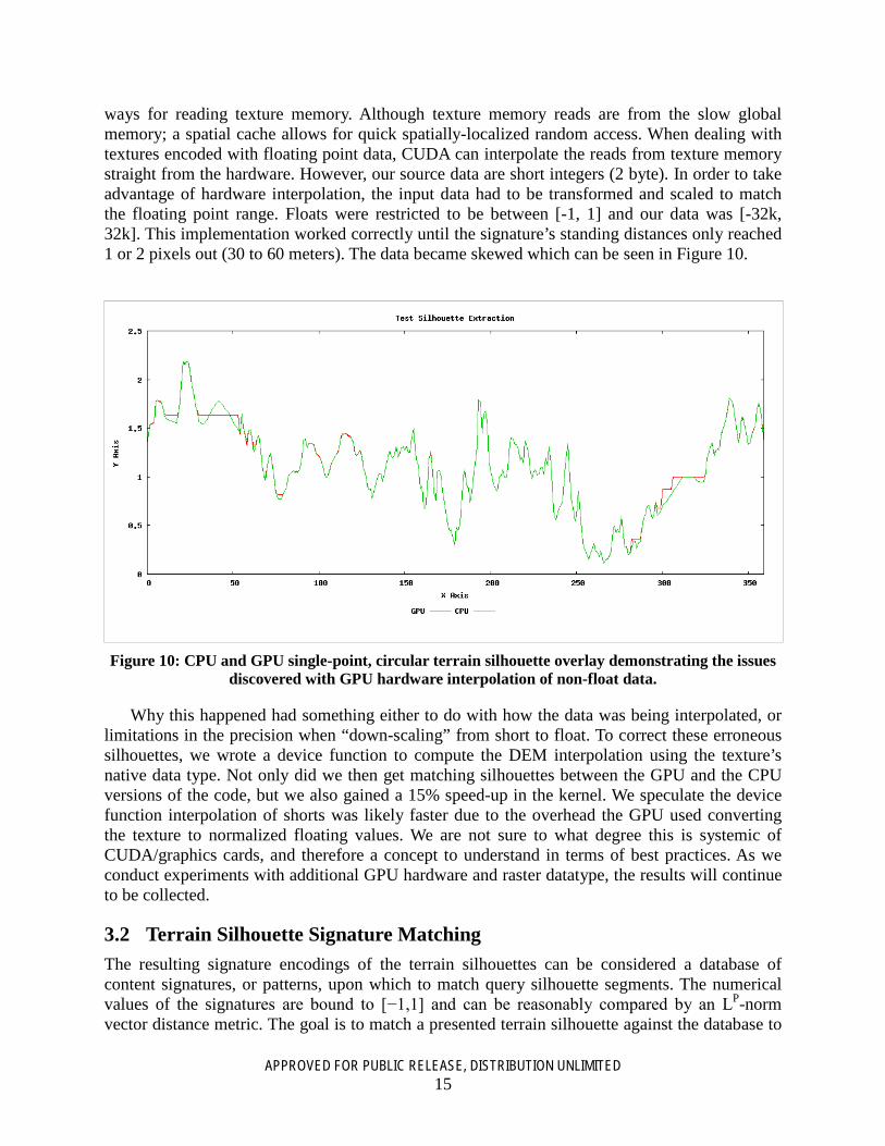
ways for reading texture memory. Although texture memory reads are from the slow global memory; a spatial cache allows for quick spatially-localized random access. When dealing with textures encoded with floating point data, CUDA can interpolate the reads from texture memory straight from the hardware. However, our source data are short integers (2 byte). In order to take advantage of hardware interpolation, the input data had to be transformed and scaled to match the floating point range. Floats were restricted to be between [-1, 1] and our data was [-32k, 32k]. This implementation worked correctly until the signature’s standing distances only reached 1 or 2 pixels out (30 to 60 meters). The data became skewed which can be seen in Figure 10.
Figure 10: CPU and GPU single-point, circular terrain silhouette overlay demonstrating the issues discovered with GPU hardware interpolation of non-float data.
Why this happened had something either to do with how the data was being interpolated, or limitations in the precision when “down-scaling” from short to float. To correct these erroneous silhouettes, we wrote a device function to compute the DEM interpolation using the texture’s native data type. Not only did we then get matching silhouettes between the GPU and the CPU versions of the code, but we also gained a 15% speed-up in the kernel. We speculate the device function interpolation of shorts was likely faster due to the overhead the GPU used converting the texture to normalized floating values. We are not sure to what degree this is systemic of CUDA/graphics cards, and therefore a concept to understand in terms of best practices. As we conduct experiments with additional GPU hardware and raster datatype, the results will continue to be collected.
3.2 Terrain Silhouette Signature Matching The resulting signature encodings of the terrain silhouettes can be considered a database of content signatures, or patterns, upon which to match query silhouette segments. The numerical values of the signatures are bound to [−1,1] and can be reasonably compared by an LP-norm vector distance metric. The goal is to match a presented terrain silhouette against the database to

APPROVED FOR PUBLIC RELEASE, DISTRIBUTION UNLIMITED 16
determine the geolocation which would produce the query terrain silhouette. One of the issues that must be addressed is the lack of scale information, e.g., is the presented silhouette equivalent to one, one and half, two, or more Θ sized windows. To overcome this unknown scale issue, the query can be sampled at numerous granularities and as multiple windows, as partially demonstrated in Figure 11. Each window that is sampled into the fixed encoding size may register a match against an existing segment in the database. These matches represent a position and orientation, which can then be spatially aggregated into probability weighted regions of geolocation. This is our demonstration interface’s point of weakness and area that requires additional research and development. Specifically, the generation of query signatures from the user-traced line on an image continue to have issues generating consistent query vectors. Due to the high resolution of images, when converting from pixel-space into a query vector, we must aggregate sets of pixels in the image. This is for the following two reasons: pixel-to-pixel transitions are very granular in the raster domain, and the change in the x-dimension is an unknown angular partial degree of the field of view. For example, depending on the resolution of the image and the focal characteristics of the imaging device, one angular degree may range from 2 pixels width to 100 pixels of width in the image. We attempt to mitigate this challenge by using multiple sampling strategies to generate a set of signatures from a trace line. We have developed database code, web services, and a nominal demonstration interface.

APPROVED FOR PUBLIC RELEASE, DISTRIBUTION UNLIMITED 17
Figure 11: Possible sub-query windows that can be generated from a query terrain silhouette.

APPROVED FOR PUBLIC RELEASE, DISTRIBUTION UNLIMITED 18
Figure 12: Geolocation data flow.
Figure 12 represents the high-level data flow for query linestrings. The system will automatically decompose the input linestring into a large collection of candidate segments and perform large-scale parallel matching. Each segment will generate a planar set of candidate geolocation points. These geolocation point sets are then clustered using our novel spatial–orientation–match-score mode seeking clustering algorithm (see Section 3.3).
3.2.1 Overview of signature matching We have developed a geolocation capability that functions as a web service. Other web services provide metadata about geolocation datasets, such as what data sets are available, their size and spatial extents. These web services provide data for the demonstration interface; both the web demonstration interface and the web services are detailed in Chapter 4. Signature matching is performed via PL/pgSQL2 functions in the services schema that receive the query feature set label, the signature, and the desired result set size. The query feature set label is used as an identifier for input queries to facilitate tracking and collection during aggregation activities described in Sect. 3.3. All of our developed techniques have performed brute-force matching of the query signature against every signature in the selected data set.
2 See: http://www.postgresql.org/docs/9.3/static/plpgsql-overview.html
PL/pgSQL is a loadable procedural language for the PostgreSQL database system. The design goals of PL/pgSQL were to create a loadable procedural language that: a) can be used to create functions and trigger procedures, b) adds control structures to the SQL language, c) can perform complex computations, d) inherits all user-defined types, functions, and operators, e) can be defined to be trusted by the server.

APPROVED FOR PUBLIC RELEASE, DISTRIBUTION UNLIMITED 19
3.2.2 GPU-enabled PostgreSQL for Signature Matching
Figure 13: PostgreSQL DBMS has been extended through SPI to support high-throughput
streaming pattern matching with integrated K-nearest neighbor generation.
We have developed initial database extensions that are designed for high-throughput stream processing for pattern matching. These extensions are built as shared objects and dynamically linked into the PostgreSQL DBMS at run time. This work is being abstracted into a framework for high-throughput pattern matching from large-scale pattern databases. We have conducted a deep-dive into the internals and back-end server-side components of the PostgreSQL DBMS. We are constructing a tutorial and documentation to facilitate repeatable database extensions using the server programming interface (SPI) of PostgreSQL. Figure 13 provides an illustrative overview of our high-throughput pattern stream processing.
Our original base-line signature matching used internal database functions written in PL/pgSQL applied to the signature column of a table. The latest variation uses a set-returning function (SRF) technique to perform block processing in shared object code that has been dynamically linked into the database. The current high-throughput pattern matching technique is 75% faster than the baseline matching function. We expect further improvements as we continue to refine our code and understanding of the PostgreSQL backend.
To accomplish this, we have researched and utilized the PostgreSQL SPI support for returning sets (multiple rows) from a C-language function. A SRF must follow the version-1

APPROVED FOR PUBLIC RELEASE, DISTRIBUTION UNLIMITED 20
calling conventions [3] and the source files must include funcapi.h. A standard SRF is called once for each item it returns. The SRF must therefore save enough state to remember what it was doing and return the next item on each call. Heuristically speaking, the PostgreSQL documentation explains C-based SRF as a branching function that uses SRF_IS_FIRSTCALL() to differentiate the primary and subsequent calls to a SRF (handled by the SPI framework). The initial call will execute a function or block of code based on SRF_IS_FIRSTCALL() to setup all data and memory contexts then ultimately return the first row, while each subsequent call ignores the setup block and returns the next result row until the end is reached (which requires another branching statement). All this additional work, may or may not improve performance beyond a simple PL/pgSQL that invokes a C-based function. This was NOT tested, because of other user experiences related in the PostgreSQL forums.
Alternatively, there exist another form of SRF which better supports our desired pattern stream processing, Block SRF. This concept is generally undocumented, except in PostgreSQL source code [4] and the occasional discussion thread topics in the PostrgeSQL Hacker’s Forum. Our working example from which we based our development was the PostgreSQL crosstab table expression functions [5]. Instead of using first-call logic to initialize state then start returning rows (i.e., analogous to a standard cursor); it instead builds a materialized table in a memory context [4]. This materialized table is fully composed and populated as a tuple store [3] within the single call to to the function. This is an important concept as our work continues, as we believe it will facilitate better utilization of the GPU co-processor to formulate pattern matching results.
A key element of stream processing large-scale pattern recognition databases is our ability to capture the K-nearest neighbors from the stream. The original technical approach was to (a) perform parallel signature matching into score blocks, then (b) push each block through a sorting network. During the course of our work and our exploratory research into the internals of PostgreSQL DBMS, we developed an alternative technical approach to generate the top K matches from a stream of pattern signatures. Our new approach, nominally referred to as the k-sieve, provides a drastically more efficient memory usage pattern by developing a shared object memory structure that filters the stream of scored patterns into a sorted list of the best K matches.
Further extension will explore pruning and content-based retrieval techniques. The overall goal of applying these techniques is to drastically reduce the number of signatures that must be moved from the database to the GPU co-processors. As the movement of the signatures from the database (disk) to the GPU is the current bottle-neck of the matching process, we expect significant pay-off from these future efforts.
3.3 Clustering of a Geolocation Point Set In order to geolocate from a query signature extracted from a perspective image, the system begins by producing an initial hit point set of size N. Specifically, for each hit, the system generates a match score (descriptor dissimilarity value), hit location (latitude and longitude) and orientation (degrees). The challenge is to not consider each candidate in isolation, but instead consider the candidate geolocations in the context of one another. Based on our research hypothesis, we expect a quality geolocation to be supported by multiple surrounding hits with similar match scores and orientations (i.e., due to small latitude / longitude offsets and orientations). However, our initial hit list does not consider any of this contextual information. This is why the following detailed aggregation technique is critical to the overall geolocation process. The following sub-sections detail the refinement of an initial point set according to two

APPROVED FOR PUBLIC RELEASE, DISTRIBUTION UNLIMITED 21
key concepts; spatial and orientation similarity. While spatial and orientation similarity can be utilized directly within a clustering algorithm, we elected to first refine the initial match score spatial set.
3.3.1 Weighted Mean Shift Clustering The initial clustering algorithm explored for candidate geolocation point set aggregation is a variant of Mean Shift Clustering [11][27]. Mean shift clustering is a well known and widely used as a mode seeking technique. Specifically, we use a novel weighted extension of mean-shift clustering. As stated above, our geolocation aggregation task is different in the sense that clusters are not typical – in the academically formulated regard. Instead, geolocation clusters can be rather sparse and take on somewhat unique shapes (e.g., line-like segments or elongated ellipses). However, one thing appears to be consistent among the observed geolocation clusters; clusters are relatively dense and grouped in the feature space. A classical partition seeking algorithm, e.g., K-means, fuzzy C-means, etc., is insufficient for this task [28]. In particular, outliers are extremely common and they may need to be represented and identified. A number of algorithms could have been utilized for this task; such as possibilistic C-means (PCM) [14] and the robust competitive agglomerate (RCA) algorithm [12]. However, algorithms such as the PCM require a user to specify different parameters, e.g., q (fuzzifier), η, etc., which can be difficult to estimate in general. In comparison, the mean shift clustering algorithm is better suited for our particular geolocation task. That is, its free parameters (e.g., window radius) are easier to establish in the spatial context of our geolocation point sets. However, one natural consequence of this approach is the fact that multiple modes can be returned for a single perceptual cluster. This will require a post-clustering linkage to generate the desired geolocation confidence regions from the geolocation candidate list.
APPROVED FOR PUBLIC RELEASE, DISTRIBUTION UNLIMITED 22
3.3.2 Point Set Filtering: Spatial Similarity
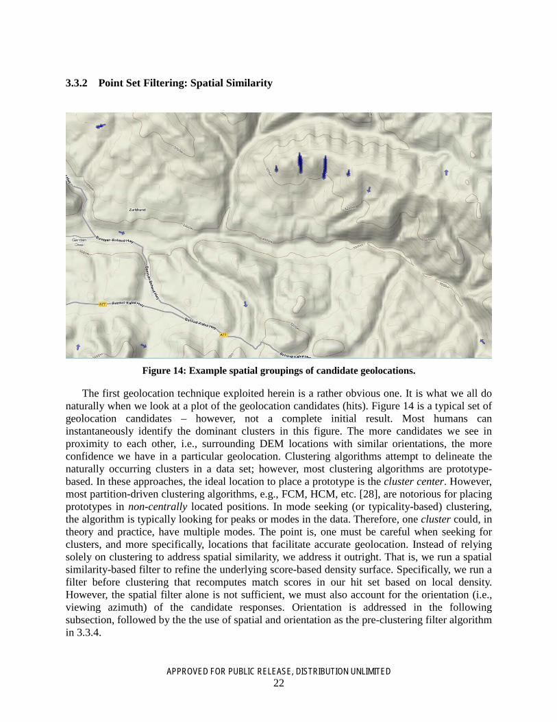
Figure 14: Example spatial groupings of candidate geolocations.
The first geolocation technique exploited herein is a rather obvious one. It is what we all do naturally when we look at a plot of the geolocation candidates (hits). Figure 14 is a typical set of geolocation candidates – however, not a complete initial result. Most humans can instantaneously identify the dominant clusters in this figure. The more candidates we see in proximity to each other, i.e., surrounding DEM locations with similar orientations, the more confidence we have in a particular geolocation. Clustering algorithms attempt to delineate the naturally occurring clusters in a data set; however, most clustering algorithms are prototype-based. In these approaches, the ideal location to place a prototype is the cluster center. However, most partition-driven clustering algorithms, e.g., FCM, HCM, etc. [28], are notorious for placing prototypes in non-centrally located positions. In mode seeking (or typicality-based) clustering, the algorithm is typically looking for peaks or modes in the data. Therefore, one cluster could, in theory and practice, have multiple modes. The point is, one must be careful when seeking for clusters, and more specifically, locations that facilitate accurate geolocation. Instead of relying solely on clustering to address spatial similarity, we address it outright. That is, we run a spatial similarity-based filter to refine the underlying score-based density surface. Specifically, we run a filter before clustering that recomputes match scores in our hit set based on local density. However, the spatial filter alone is not sufficient, we must also account for the orientation (i.e., viewing azimuth) of the candidate responses. Orientation is addressed in the following subsection, followed by the the use of spatial and orientation as the pre-clustering filter algorithm in 3.3.4.

APPROVED FOR PUBLIC RELEASE, DISTRIBUTION UNLIMITED 23
3.3.3 Point Set Filtering: Orientation Similarity While clusters of dense points with spatial similarity is naturally addressed to some extent in most clustering algorithms, our geolocation candidates’ orientation is not. While some algorithms and approaches simply concatenate all features in a system; this is not always a suitable solution. For example, in image segmentation, many elect to create a 5-dimensional feature vector that consists of (r,g,b,x,y), i.e., red, green, blue, and spatial coordinates (x,y). This concatenation creates a new Cartesian space which allows one to co-search for color similarity in conjunction with spatial similarity. We could have simply constructed a data set as follows, (x,y,o,s), where (x,y) are spatial geolocation parameters, o is the orientation and s is the match score. However, (x,y), o and s live at very different scales. Instead of naively concatenating all features together, engaging in some normalization technique, and then pushing the problem off to the clustering algorithm; we instead address orientation similarity in its own right. Specifically, our pre-clustering filter recomputes match scores in our hit set. We want to model the following behavior. The higher the orientation similarity, the more confidence one should have that a particular pair of geolocation candidates that are nearly co-located are similar. The two concepts, spatial and orientation filtering, are combined alongside the initial match scores. The next sub-section outlines the combined procedure.
3.3.4 Pre-Clustering Filter: Point Set Score Refinement
(a) (b)
Figure 15: Example of geolocation point set data and refinement: (a) top-500 query matches as a
scatter plot, (b) and the refined density surface. The circle is the true geolocation.
As discussed above, we wish to geolocate based on spatial and orientation similarity. The following steps describe pre-clustering match score refinement. Note, this filter is a re-estimation of the underlying probability density surface.

APPROVED FOR PUBLIC RELEASE, DISTRIBUTION UNLIMITED 24
Step 1 For each hit, hi, we search a local neighborhood, e.g., 9x9 window in the DEM, and build a set, Li, which are all spatially close hits.
Step 2 For each neighbor-hit in Li, i.e., gk, we compute the cosine similarity, ck, between hi and gk. Note, we clamp the value ck between [0,1], vs. [−1,1]. We also calculate a spatial similarity value,
( ),h,gf=s ik1k (8)
where f1 is a metric that operates on the hits’ corresponding latitude / longitude values. A number of similarity values could have been used (e.g., LP-norm based, EMD, exponential, etc.). Herein we use Euclidean distance3, and normalize it by the maximum distance in the neighborhood. Next, we take 1 minus this distance value to obtain a [0,1] similarity value which is one-valued only at the window center location.
Step 3 For each neighbor-hit in Li, i.e., gk, we calculate a temporary weighted score, tk, as follows
( ) ( ).12 ikkikk h,gfg,hfc=t ∗∗ (9)
Specifically, we use maximum for f2 (an optimistic operator), which is an aggregation function of the two corresponding initial match scores. However, our initial match scores are distances. First, we identify the maximum and minimum distances in the list of N points. We then normalize the distances to be between [0,1]. Next, we take 1 minus this value to obtain a similarity. The value used represents the relative–to the N hits–geolocation match strength. Each tk, therefore represents the following. It is the weighted evidence that tk is close to hi and shares similar orientation. The final value, mi, is the sum of these different tk scores. The result is a re-estimated proability density surface with respect to the N initial geolocations. It has been refined to prefer dense regions of similar orientations and avoid outliers. Figures 15 and 16 illustrate the filtered space and mean shift clustering results. Algorithmically, the geolocations are refined using the equations above into a density surface M, such that
i
ikgki h;
Lt=m ∀
∈∑ (10)
Figure 16 show an original geolocation candidate point set, followed by the refined density surface.
3 Since the spatial window that is used is only 9x9 DEM cells, this Euclidean metric is sufficient–without accounting for Earth geodesic characteristics based on latitude.

APPROVED FOR PUBLIC RELEASE, DISTRIBUTION UNLIMITED 25
(a)
(b)
Figure 16: Example of geolocation point set data and its refinement: (a) top-500 query matches as a
scatter plot, (b) and the refined density surface. The circle is the true geolocation.
3.3.5 Aggregating Clusters During our integration and analysis of the geolocation candidate clustering and derived polygons, we noted that the algorithm often generated a series of line strings instead of polygons. This tendency can be observed in the various preceding figures of this chapter. When we examined these spatially and orientationaly similar line strings that were generated, it was determined that the aggregation algorithm should merge these line strings into larger clusters. The revised, and final, geolocation candidate aggregation process is as follows:

APPROVED FOR PUBLIC RELEASE, DISTRIBUTION UNLIMITED 26
1. Pre-Clustering Filters (sect. 3.3.4);
2. Weighted Mean-Shift Clustering (sect. 3.3.1);
3. Aggregation of Cluster Centroids (new addition)
4. Polygonization of Clustered Points
Figure 17 demonstrates the results of the full result candidate clustering process. From the hundreds of initial candidates of various orientations and similarities, the results are reduced to eight clusters.
(a)
(b)
Figure 17: Example of the geolocation candidates as they are clustered. (a) shows the geolocation candidates; (b) shows the final result after the clusters are merged.

APPROVED FOR PUBLIC RELEASE, DISTRIBUTION UNLIMITED 27
3.4 Alternative Metric Investigation This section describes a graphics processor unit (GPU) based implementation in the NVIDIA CUDA programming language of the earth movers distance (EMD), a parametric proximity metric. The EMD is explored in this DARPA project for advanced dissimilarity (distance) calculation. Let h be a (one dimensional) histogram (descriptor) of length L1, and let g be a second histogram of length L2. In this DARPA project, h and g are two silhouette descriptors (from an image or digital elevation model (DEM)). Specifically, h is a silhouette descriptor from the new query image (there may be many of them due to partial matching due to occlusion or other factors) and g is a stored silhouette descriptor from the database (thus there are potentially billions or more of stored descriptors that have to be matched against in a given geospatial region). However, in general descriptors can be a number of things in the generic pattern recognition sense, such as one of numerous familiar image descriptors such as the (in)famous histogram of gradient (HOG) descriptors. One problem is bin-based distance measures can often be overly harsh. Bin-based distance measures require (so the two descriptors must be of equal length) and d(h,g) is calculated strictly between corresponding hi and gi (versus utilization of differences across hi and gj where i≠j). For example, two terrain silhouettes can be amazingly close to a human (thus, perceptually) yet fail to map to a desired distance for the family of LP-norms (e.g., Manhattan or city block distance, Euclidean distance, etc). The family of LP-norms are
( ) | | ,pgh=gh,dD
i=
piipL
1
1
−∑ (11)
thus p=1 is Manhattan city block distance, p=2 is Euclidean, p=∞ is maximum. In terms of silhouette descriptors, h could be of length L1=30 and g could be of length L2=60 (so half the angle and double the number of measurements) or L2=41 (some non-integer multiple that is more difficult to address). The lengths can be anything that the application desires. Bin-based matching could still possibly work in the integer-multiple case above if we “conditioned” h, e.g., doubled its “resolution” and used interpolation. However, it is not clear how the non-integer bin case should be handled (possible re-sampling as the two histograms are simply not sampled at the same “rate”). In the case that bins do not have simple underlying meanings, this becomes drastically more difficult. For example, if descriptors are bag of words (visual) descriptors, one may desire to represent a different potentially unique distance when determining the difference between one in (visual descriptor) and another bin. The EMD is an extremely flexible system that can be tailored to numerous tasks. Specifically, in this work the EMD is being explored to address subtle shifts in the mass in the descriptor. Silhouettes are not always accurately segmented from variable resolution imagery and based on the resolution (meter spacing) of a digital elevation model (DEM) “natural” domain differences are likely to emerge. One needs a distance measure that can handle, with grace, such domain challenges. The EMD is also able to address the case of unequal mass descriptors. For example, it can obviously do matching between two probability distributions, but it can also match two general distributions in which
.

APPROVED FOR PUBLIC RELEASE, DISTRIBUTION UNLIMITED 28
As an example, consider the following simple histogram matching example. Assume h=(.7,0,0,.3,0), g1=(0,.7,0,0,.3) and g2=(.2,.2,.2,.2,.2). Figure 18 illustrates these three histograms. According to a LP-norm, h and g2 are more similar than h and g1. However, g1 is really just a single bin shifted version of h and g2 is clearly a uniform distribution. This is a simple numeric example for a low dimensional case (D=5), but when the descriptors are longer (e.g., D=128) and the shifts are subtle (e.g., single bin shift), the differences from a LP can be very extreme while the distributions are only slightly different. Of course, this depends on the underlying feature space corresponding to the descriptor (thus interpretation of what bin-to-bin dissimilarity means). According to the LP-norm, there is no similarity between h and g1 as no bins have anything in common. However, there is similarity between h and . Specifically, g2 would be preferred to g1, with respect to h. We need some way to capture that there is indeed some similarity between h and g1.
Figure 18: Three extremely simple example histograms. Which do you think are more similar? (a)
is h=(.7,0,0,.3,0), (b) is g1=(0,.7,0,0,.3) and (c) is g2=(.2,.2,.2,.2,.2).
The EMD measures the amount of “work” it takes to “transform” one descriptor into another. It relies on solving an underlying optimization (transportation) problem. This must be solved for each distance calculated. This is time consuming and can be a deal breaker for many applications. In this research, the EMD is used to better capture the perceptual difference between two silhouette descriptors. It is the belief of this team that it is an important part of the proposed system. Therefore, we have engaged in a GPU-based solution to the EMD to speed it up. Specifically, we rely on a solution to (algorithm for) the underlying transportation simplex problem. There are other theoretically faster solutions (discussed below) that we will visit in the future if we have the time and need. However, they are a (relatively) major time investment (more so than the proposed algorithm). The following sections describe the EMD, our GPU implementation and the application specific details.
3.4.1 Earth Mover’s Distance The EMD has been explored in a number of works in machine learning and computer vision. The EMD aims to measure the perceptual equivalence between two potentially variable size descriptions of distributions. Herein, without loss of generality, we refer to these descriptors as histograms. However, the underlying distributions could be probabilistic, possibilistic, image descriptors, etc. The EMD is based on a solution to the well-known transportation problem, aka Monge-Kantorovich problem. In [29], Rubner introduced the EMD, and the well-known signature form, in the context of content based image retrieval (CBIR). In [30], Levina and Bickel proved that the EMD is the Mallows distance for two probability distributions. However, as Levina and Bickel observed, the Mallows and EMD behave differently for the case of two

APPROVED FOR PUBLIC RELEASE, DISTRIBUTION UNLIMITED 29
histograms (or signatures) with different masses. Specifically, the EMD has the advantage that it allows for partial matching. This feature is important in the case of CBIR. The goal of the EMD is to find a flow F=[fij], where is the flow between hi and gj, that minimizes the overall cost
( ) ,fd=Fg,h,WORK ij
L
=i
L
j=ij∑∑
1
1
2
1
(12)
subject to the constraints
,LjLi;fij 21,110 ≤≤≤≤≥ (13)
,Li;hf i
L
j=ij 1
2
11 ≤≤≤∑ (14)
,Lj;gf j
L
=iij 2
1
11 ≤≤≤∑ (15)
,g,hmin=fL
j=j
L
=ii
L
=i
L
j=ij
∑∑∑∑
1
1
2
1
2
1
1
1
(16)
where D = [dij] is the ground distance matrix. For example, the most common ground distance is
( ),ji=dij − (17)
Intuitively, the EMD can be thought of as follows. Imagine that the two histograms are piles of sand or earth sitting on the ground. Then the distance between the two piles can be thought of as how far the grains of sand have to be moved to make one pile be transformed into the other. That is, the EMD is the minimal total ground distance traveled weighted by the amount of sand moved. Once the transportation problem is solved [29], and the optimal is found, the EMD is calculated as follows
( ) .ˆ
ˆ
2
1
1
1
1
1
2
1
∑∑
∑∑L
=i
L
j=ij
ij
L
=i
L
j=ij
f
df=g,h,EMD (18)
The normalization in Equation 18 is the total weight of the smaller histogram (Constraint 16). This is required when two histograms have different total weight (avoids favoring the smaller histogram). While the ground distance can be, in general, any distance, different selections result in different properties (e.g., measure or metric properties). Specifically, if the two histograms have equal mass and the ground distance is a metric, then the EMD is a metric. This means is satisfies important properties such as symmetry, reflexivity, triangular inequality, etc.

APPROVED FOR PUBLIC RELEASE, DISTRIBUTION UNLIMITED 30
4 GEOLOCATION WEB SERVICES AND DEMONSTRATION UI
Figure 19: Demonstration web user interface.
To demonstrate an initial capability, we developed a basic web user interface. This interface, shown in Figure 19, allows a user to perform an assisted tracing of the terrain silhouette, then automatically partitions the traced line into the ten most variable segments as candidates for geolocation. Figure 20 shows the general flow of this prototype user interface. The web interface is designed to utilize a collection of component web services, using AJAX techniques to render the page and process geolocation related activities. This section details the components of the demonstration web user interface and how these components interact with the supporting web services.

APPROVED FOR PUBLIC RELEASE, DISTRIBUTION UNLIMITED 31
Figure 20: Web UI flowchart.

APPROVED FOR PUBLIC RELEASE, DISTRIBUTION UNLIMITED 32
Feature Set Selection The initial step is to select a feature set (i.e., single collection of terrain segment signatures with common collection parameters). More specifically, for a particular set of parameters, such as azimuth sampling and signature size, we materialized different database data tables. The feature set is the selection mechanism to specify which table to search against. This will allow the “Silhouette To Signature Service” to properly generate the signatures based on the type of the feature set. The parameters associated with the feature are used in subsequent steps to partition the input silhouette trace into a large set of suitable query signatures.
Scissors: Raster Based Silhouette Extraction In the second step the user will first draw a rough mask over the image to highlight the area; and then perform a computer assisted tracing of the terrain silhouette. We acquired and modified an existing open source solution to develop the capability to automatically snap the tracing to the terrain horizon. Algorithmically, edge-detectors and gradients are used to perform the snapping of the trace to the optimal pixels. The user may need to intervene for minor mistakes in the line snapping algorithm. After the terrain silhouette has been traced, the user can click “Add Signature” which will use an AJAX web service to send off the trace path and the feature set identifier to the “Silhouette To Signature Service”. This service will generate a collection of the most variable segment signatures, based on variability.
Silhouette Selection for Geolocation The user interface will produce a multi-colored list of candidate segments, these candidate segements can be selected to see how they overlay on the original image. The user will select the silhouettes they want to Geolocate. Silhouettes are interpolated with different techniques, e.g., sampling or averaging, for each query segment point. This allows some variability during our non-automated testing, allowing us to choose between different interpolations of similar silhouettes. Additionally, the user interface contains the computed segment signatures that can be be used for geolocation.
Geolocation Map The geolocation map will show the results of the “Geolocation Services” and the extents of the different feature sets. The map renders a polygon with a direction identifier and confidence attribute. Table 1 provides a summary and thumbnail view of each of the preceding components of the web user interface.

APPROVED FOR PUBLIC RELEASE, DISTRIBUTION UNLIMITED 33
Table 1: Web UI Components
Feature Set Selection The first step in the application is to select the feature set. This allows the “Silhouette To Signature Service” to properly generate the signatures based on the type of the feature set. The feature set represents a particular set of parameters, such as azimuth sampling and signature size that were used to materialize different database data tables. If the feature set is not selected, the user cannot pass onto the next step.
Scissors: Raster Based Silhouette Extraction The user first draws a rough mask on the image, and then draws the silhouette which will automatically snap to the proper horizon. The user may need to intervene for minor mistakes in the algorithm. Afterwards, the user clicks “Add Signature”, which sends off the feature set and the silhouette produced to the “Silhouette To Signature Service” which hands off the most useful silhouettes to the “Silhouette Selection for Geolocation”.
Silhouette Selection for Geolocation The user selects the silhouettes they want to use to geolocate. When a silhouette is selected, it is displayed on the map above. Some silhouettes are interpolated differently (nearest neighbor or averaged), so the user can choose between different interpolations of similar silhouettes. Once the silhouettes are selected, the user will click the “Geolocate” button which sends the silhouette signatures to the “Geolocation Service”.
Geolocation Map The map shows the results of the “Geolocation Services” and the extents of the different feature sets. Arrows are rendered for every hit in this image for visualization purposes.
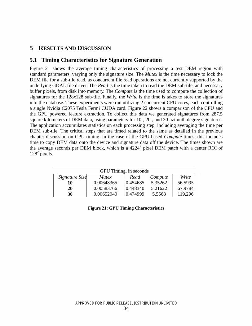
APPROVED FOR PUBLIC RELEASE, DISTRIBUTION UNLIMITED 34
5 RESULTS AND DISCUSSION
5.1 Timing Characteristics for Signature Generation Figure 21 shows the average timing characteristics of processing a test DEM region with standard parameters, varying only the signature size. The Mutex is the time necessary to lock the DEM file for a sub-tile read, as concurrent file read operations are not currently supported by the underlying GDAL file driver. The Read is the time taken to read the DEM sub-tile, and necessary buffer pixels, from disk into memory. The Compute is the time used to compute the collection of signatures for the 128x128 sub-tile. Finally, the Write is the time is takes to store the signatures into the database. These experiments were run utilizing 2 concurrent CPU cores, each controlling a single Nvidia C2075 Tesla Fermi CUDA card. Figure 22 shows a comparison of the CPU and the GPU powered feature extraction. To collect this data we generated signatures from 287.5 square kilometers of DEM data, using parameters for 10-, 20-, and 30-azimuth degree signatures. The application accumulates statistics on each processing step, including averaging the time per DEM sub-tile. The critical steps that are timed related to the same as detailed in the previous chapter discussion on CPU timing. In the case of the GPU-based Compute times, this includes time to copy DEM data onto the device and signature data off the device. The times shown are the average seconds per DEM block, which is a 42242 pixel DEM patch with a center ROI of 1282 pixels.
GPU Timing, in seconds Signature Size Mutex Read Compute Write
10 0.00648365 0.454685 5.35262 56.5995 20 0.00583766 0.448340 5.21622 67.9784 30 0.00652040 0.474999 5.5568 119.296
Figure 21: GPU Timing Characteristics

APPROVED FOR PUBLIC RELEASE, DISTRIBUTION UNLIMITED 35
Figure 22: Timing on the CPU and GPU side by side
We have made some observations and speculations regarding the timing aspects and comparison of CPU versus GPU. When the GPU does the signature computation, the CPU remains free to focus on the database sink. Additionally the CPU was run with 12 concurrent cores. The server that performed this experiment has 12 logical CPU cores, but this is on a single Intel Xeon chip. Additionally, the server that is performing the extraction is also running the PostgreSQL ODBMS server. Therefore, we expect that CPU-based signature extraction created a significant load on the machine in both CPU usage, as well as writes for the database. Additionally, based our review of timing from logs and monitoring database activity during signature generation; various database structure and signature sink changes were put in place. The overall effect is significant improvement in database related signature storage timings.
Comparing the two timing plots, it can be seen that the signature computation time is drastically faster on the GPU versus the CPU. Even though we have made improvements to the database storage of the signatures, this remains a bottleneck in the signature generation application. Further optimization efforts will be focused on the database related aspects. As a final point of reference, we computed the effective time per pixel to get a comparable number for processing given the challenge of accurately comparing twelve CPU cores versus two GPU co-processors. The CPU effective time per pixel (tpp) is 0.00787008 s; while the GPU tpp is 0.00190723 s. Using the GPU results in approximately a 4x times speedup; and we found a similar result using a four GPU co-processor server. Adding additional GPU did not accelerate the tpp in a statistically significant degree due to the bottle neck writing data to the database. Therefore, every performance increase we can derive from the database sink will increase the per-pixel throughput.

APPROVED FOR PUBLIC RELEASE, DISTRIBUTION UNLIMITED 36
5.2 Signature matching timings
Figure 23: Geolocation point set generation timings for database sizes ranging from 1m to 100m.
The Per-row SO is using a compiled shared object library function linked into the database to compute segment similarity, which is called once for each row of data. The Per-row SO + filter applies a filter to the rows, reducing the number of calls to the shared object. The PL/pgSQL is
using an internal database function written in PL/pgSQL, which is an order of magnitude slower.
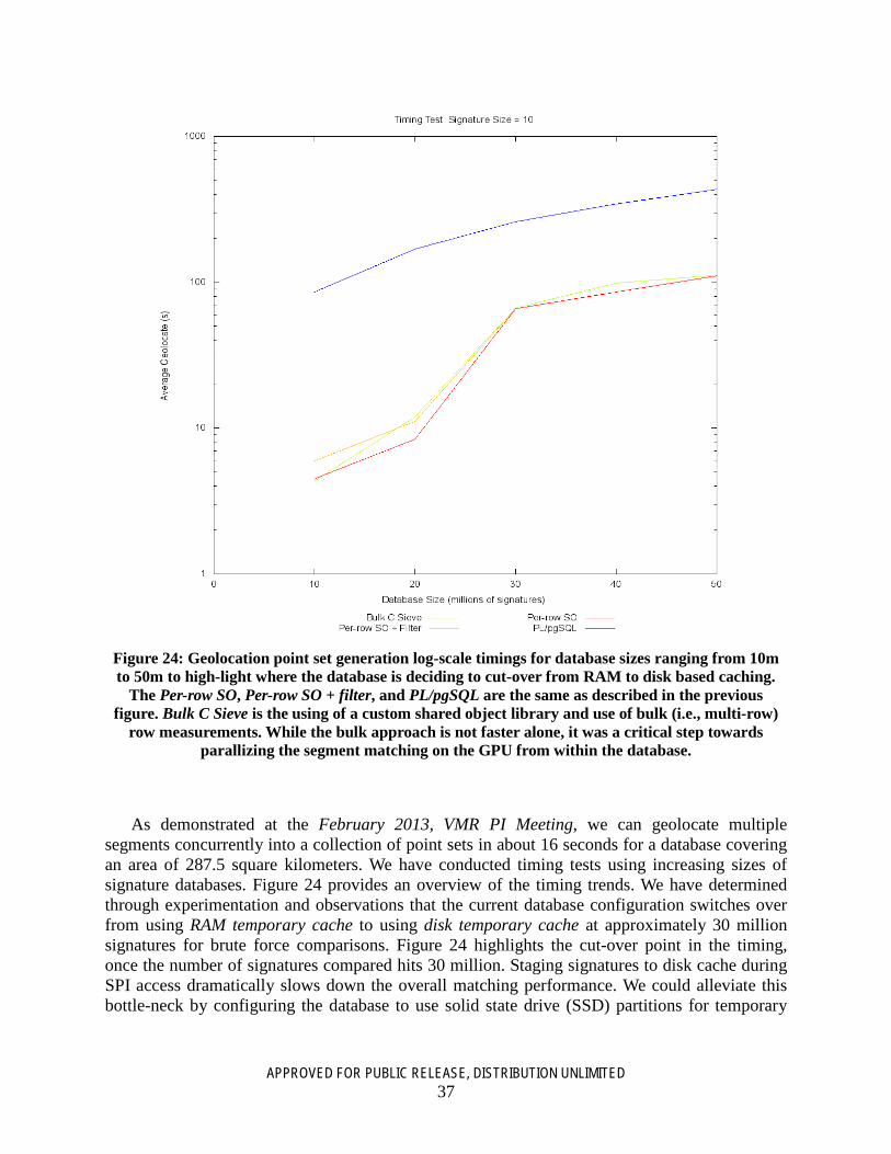
APPROVED FOR PUBLIC RELEASE, DISTRIBUTION UNLIMITED 37
Figure 24: Geolocation point set generation log-scale timings for database sizes ranging from 10m to 50m to high-light where the database is deciding to cut-over from RAM to disk based caching.
The Per-row SO, Per-row SO + filter, and PL/pgSQL are the same as described in the previous figure. Bulk C Sieve is the using of a custom shared object library and use of bulk (i.e., multi-row)
row measurements. While the bulk approach is not faster alone, it was a critical step towards parallizing the segment matching on the GPU from within the database.
As demonstrated at the February 2013, VMR PI Meeting, we can geolocate multiple segments concurrently into a collection of point sets in about 16 seconds for a database covering an area of 287.5 square kilometers. We have conducted timing tests using increasing sizes of signature databases. Figure 24 provides an overview of the timing trends. We have determined through experimentation and observations that the current database configuration switches over from using RAM temporary cache to using disk temporary cache at approximately 30 million signatures for brute force comparisons. Figure 24 highlights the cut-over point in the timing, once the number of signatures compared hits 30 million. Staging signatures to disk cache during SPI access dramatically slows down the overall matching performance. We could alleviate this bottle-neck by configuring the database to use solid state drive (SSD) partitions for temporary

APPROVED FOR PUBLIC RELEASE, DISTRIBUTION UNLIMITED 38
(e.g., scratch) table spaces. In addition to modifying database settings, we will also explore alternatives that move the matching away from brute-force comparisons.
5.3 Signature matching clustering The figures 17, 25, and 26 show three separate test cases during the geolocation candidate aggregation process. The candidate aggregation is described in detail in Section 3.3.
(a)
(b)
Figure 25: Example of the geolocation candidates as they are clustered. (a) shows the geolocation candidates; and (b) shows the final result after the clusters are merged.
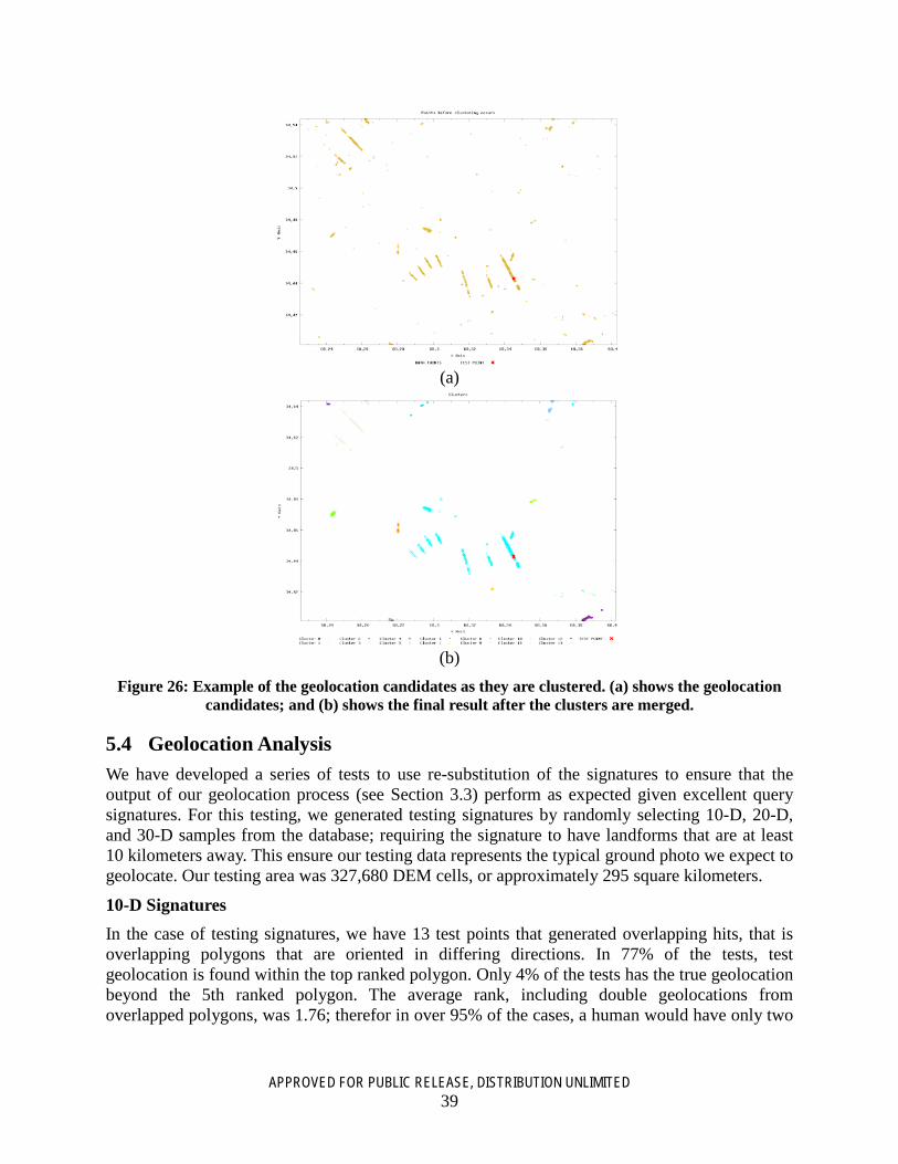
APPROVED FOR PUBLIC RELEASE, DISTRIBUTION UNLIMITED 39
(a)
(b)
Figure 26: Example of the geolocation candidates as they are clustered. (a) shows the geolocation candidates; and (b) shows the final result after the clusters are merged.
5.4 Geolocation Analysis We have developed a series of tests to use re-substitution of the signatures to ensure that the output of our geolocation process (see Section 3.3) perform as expected given excellent query signatures. For this testing, we generated testing signatures by randomly selecting 10-D, 20-D, and 30-D samples from the database; requiring the signature to have landforms that are at least 10 kilometers away. This ensure our testing data represents the typical ground photo we expect to geolocate. Our testing area was 327,680 DEM cells, or approximately 295 square kilometers.
10-D Signatures In the case of testing signatures, we have 13 test points that generated overlapping hits, that is overlapping polygons that are oriented in differing directions. In 77% of the tests, test geolocation is found within the top ranked polygon. Only 4% of the tests has the true geolocation beyond the 5th ranked polygon. The average rank, including double geolocations from overlapped polygons, was 1.76; therefor in over 95% of the cases, a human would have only two

APPROVED FOR PUBLIC RELEASE, DISTRIBUTION UNLIMITED 40
polygon areas to examine. The average polygon area of the geolocations was 6.37 square kilometers, a 97.8% reduction in the geolocation search space.
5.5 Human Perspective Matching During the course of this project, the human perspective matching was determined to be of minor interest to the VMR program during a meeting with the VMR program manager. The project instead focused on alternatives related to database organization and management of signatures for matching to improve scalability and performance. However, initial work was conducted towards this goal, resulting in the basic ability to render the geolocation candidates using an open source 3-D rendering library (OGRE4), DEM data, and NASA Landsat satellite imagery5.
Figure 27 shows the processing flow of the rendering of geolocation candidates. Figure 28 shows the rendering of a DEM region from an elevated perspective in (a) and from the ground perspective in (b).
Figure 27: Overview perspective rendering process flow.
4 OGRE: http://www.ogre3d.org/ 5 Landsat is a global satellite imagery coverage data set that is low resolution, similar to the ground sample distance of the DEM data. http://landsat.gsfc.nasa.gov/

APPROVED FOR PUBLIC RELEASE, DISTRIBUTION UNLIMITED 41
(a)
(b)
Figure 28: Example renderings of a geolocation position from (a) arbitrary position and (b) from the actual perspective position.
APPROVED FOR PUBLIC RELEASE, DISTRIBUTION UNLIMITED 42
6 CONCLUSIONS & RECOMMENDATIONS This research has demonstrated the potential to achieve geolocation of terrain silhouettes in ground photos when adequate query traces are generated and used against the system. The search space reduction, as a result of search the output geolocation polygons is typically more than 95%. Our demonstration user interface has over 74,000 square kilometers of Afghanistan ingested, precisely 82,575,360 SRTM DTED Level 2 DEM cells. The system is capable of searching this area in 13 minutes and 35 seconds using a single query, which is a search rate of 91.18 square kilometers a second using a single GPU device integrated into the database.
In addition to this proof-of-concept capability, several of the novel technologies we developed as part of this effort have wider ranging applications. We have developed the first, as far as we know, integration of GPU hardware and database management system software for large-scale pattern matching. The technologies offer many promising benefits in a variety of fields that rely on pattern recognition techniques, ranging from content-based image retrieval to computer vision to biometrics. We will be exploring each of these topics in the future. Additionally, our geospatial data processing architecture represents one of the first wholistic treatements of large-scale geodata processing with GPU acceleration.
6.1 Recommendations Our general approach to materializing the terrain silhouettes signatures into the database represents a great technique if the geolocation searches can be coupled with auxillary spatial or relational filtering information. For instance, if an analyst using a system with this capability can constrain the geolocation search to an particular geospatial region based on cultural characteristics, it would greatly reduce the search space. This approach directly exploits the advantages and power of the database engine. However, using our approach in isolation from other data leaves only the overhead of the database as a contributing factor. In scenarios such as this, there are potentially better alternatives to storing the signatures, such as large scale distributed file system or distributed NoSQL with custom data processing. The most critical issue to resolve is the development of good signature extraction techniques for the ground photos. Matching the samplings of the DEM to the ground photos’ varied resolutions continues to be an issue that hampers matching.
One potential approach to leverage other data as well as mitigate the the cost of storing the signatures within the database would be to use geospatial analysis to select regions for real-time terrain silhouette analysis. The existing work of aggregating geolocation candidates is developed as a library outside of the database, and could therefore be leveraged against this alternative approach. Additionally, we believe this approach will give more flexibility to try a variety of sampling of azimuth during extraction from the DEM as well as the image to improve results.
It should be noted that the government has dedicated considerable resources (10’s of millions of dollars) to other geolocation approaches, such as Finder6. While it is unlikely that this project will find further interest beyond this effort, code developed during this effort has already been shared to some of the contractors that were on both the VMR and the Finder projects.
6 IARPA Finder: http://www.iarpa.gov/index.php/research-programs/finder/baa

APPROVED FOR PUBLIC RELEASE, DISTRIBUTION UNLIMITED 43
7 BIBLIOGRAPHY [1] http://www.gdal.org/ogr/index.html. [2] http://www.gdal.org/. [3] http://www.postgresql.org/docs/9.2/static/spi.html. [4] http://anoncvs.postgresql.org/cvsweb.cgi/pgsql/src/backend/utils/mmgr/README?rev=1.15. [5] http://doxygen.postgresql.org/tablefunc_8c.html#a29b9ff7ae5c29cc057658cecaad19b71. [6] Georges Baatz, Olivier Saurer, Kevin Köser, and Marc Pollefeys. Large scale visual geo-localization of images in mountainous terrain. In Proceedings of the 12th European conference on Computer Vision - Volume Part II, ECCV’12, pages 517–530, Berlin, Heidelberg, 2012. Springer-Verlag. [7] Lionel Baboud, Martin Cadik, Elmar Eisemann, and Hans-Peter Seidel. Automatic photo-to-terrain alignment for the annotation of mountain pictures. In Computer Vision and Pattern Recogntion, 2011. Proceedings., IEEE, pages 41–48, jun 2011. [8] R. Behringer. Registration for outdoor augmented reality applications using computer vision techniques and hybrid sensors. In Virtual Reality, 1999. Proceedings., IEEE, pages 244–251, mar 1999. [9] Reinhold Behringer. Improving the registration precision by visual horizon silhouette matching. In Proceedings of the First IEEE Workshop on Augmented Reality, 1998. [10] Yann Chevriaux, Eric Saux, and Christophe Claramunt. A landform-based approach for the representation of terrain silhouettes. In Proceedings of the 13th annual ACM international workshop on Geographic information systems, GIS ’05, pages 260–266, New York, NY, USA, 2005. ACM. [11] Dorin Comaniciu, Peter Meer, and Senior Member. Mean shift: A robust approach toward feature space analysis. IEEE Transactions on Pattern Analysis and Machine Intelligence, 24:603–619, 2002. [12] H. Frigui and R. Krishnapuram. A robust clustering algorithm based on competitive agglomeration and soft rejection of outliers. In Computer Vision and Pattern Recognition, 1996. Proceedings CVPR ’96, 1996 IEEE Computer Society Conference on, pages 550–555, 1996. [13] D.B. Goldgof, T.S. Huang, and H. Lee. A curvature-based approach to terrain recognition. 11(11):1213 –1217, nov 1989. [14] R. Krishnapuram and J.M. Keller. The possibilistic c-means algorithm: insights and recommendations. Fuzzy Systems, IEEE Transactions on, 4(3):385–393, 1996. [15] Lars Kulik and Max Egenhofer. Linearized terrain: Languages for silhouette representations. In Walter Kuhn, Michael Worboys, and Sabine Timpf, editors, Spatial Information Theory. Foundations of Geographic Information Science, volume 2825 of Lecture Notes in Computer Science, pages 118–135. Springer Berlin / Heidelberg, 2003. [16] R. Lerner and E. Rivlin. Direct method for video-based navigation using a digital terrain map. 33(2):406–411, feb 2011. [18] NIMA. Performance specification digital terrain elevation data (dted), May 2000.

APPROVED FOR PUBLIC RELEASE, DISTRIBUTION UNLIMITED 44
[19] S.W. Pritt. Geolocation of photographs by means of horizon matching with digital elevation models. In Geoscience and Remote Sensing Symposium (IGARSS), 2012 IEEE International, pages 1749–1752, 2012. [20] J.J. Rodriguez and J.K. Aggarwal. Matching aerial images to 3-d terrain maps. 12:1138–1149, 1990. [22] G. Scott and Chi-Ren Shyu. Knowledge-driven multidimensional indexing structure for biomedical media database retrieval. Information Technology in Biomedicine, IEEE Transactions on, 11(3):320–331, may 2007. [23] G.J. Scott, M.N. Klaric, C.H. Davis, and Chi-Ren Shyu. Entropy-balanced bitmap tree for shape-based object retrieval from large-scale satellite imagery databases. Geoscience and Remote Sensing, IEEE Transactions on, 49(5):1603–1616, may 2011. [24] Grant Scott, Matt Klaric, and Chi-Ren Shyu. Modeling multi-object spatial relationships for satellite image database indexing and retrieval. In Image and Video Retrieval, volume 3568 of Lecture Notes in Computer Science, pages 590–590. Springer Berlin / Heidelberg, 2005. [25] Chi-Ren Shyu, Pin-Hao Chi, Grant Scott, and Dong Xu. Proteindbs: a real-time retrieval system for protein structure comparison. Nucleic Acids Research, 32(suppl 2):W572–W575, 2004. [26] F. Stein and G. Medioni. Structural indexing: Efficient 2d object recognition. 14:1198–1204, 1992. [27] K. Stone, J. M. Keller, D. T. Anderson, and D. B. Barclay. An automatic detection system for buried explosive hazards in fl-lwir and fl-gpr data. Proc. SPIE 8357, Detection and Sensing of Mines, Explosive Objects, and Obscured Targets XVII, page doi:10.1117/12.920288, 2012. [28] Sergios Theodoridis and Konstantinos Koutroumbas. Pattern Recognition, Fourth Edition. Academic Press, 4th edition, 2008. [29] Rubner, et. al, The Earth mover's distance as a metric for image retrieval. International Journal of Computer Vision, 40, 2000. [30] Levina and Bickel. The earth mover's distance is the mallows distance: Some insights from statistics. International Conference on Computer Vision, pp 251-256, 2001.

APPROVED FOR PUBLIC RELEASE, DISTRIBUTION UNLIMITED 45
APPENDIX: CONTRACT EXTENSION REPORT
Evaluation of GPU-accelerated DBMS for VMR DIG This sub-report covers the contract extension period for effort FA8750-12-C-0018, GPU-accelerated DBMS for terrain geolocation with human view verification, for the period of 1 OCT 2014 to 1 JAN 2015. The scope of this extension was as follows:
Provide support for the VMR Database Index Working Group (DIG) to assess the use of SQL database technology for image queries.
The following three primary assessment tasks were identified in the revised statement of work:
1. Benchmark query throughput for direct SIFT feature matching, scaling up to at least 10,000,000 vectors.
2. Benchmark query throughput for queries restricted by object bounding boxes, specifically vehicles and people.
3. Explore performance improvement by encoding feature matching indices in SQL, such as hash tree.
We have completed all the tasks, and performed various testing and analysis exercises. Each task is allocated a detailed section in the following document. As a high-level summary we offer the following insight.
Our integration of GPU co-processor hardware offers substantial acceleration of pattern analysis tasks when the data can be directly streamed from the DB storage to the GPU. However, usage patterns that exploit intermediate table expressions to produce the data stream for the GPU seem to incur a cost that was rarely overcome in our testing scenarios. This implies that the pattern database must be a massive data set, and the stream pre-filtering must significantly reduce the input pattern stream size to achieve measurable benefits on the front-side of the pattern stream. However, in the post-filter scenario we see costs that are dominated by the pattern stream analysis, and as such the exploitation of the auxiliary filtering incurs little relative costs. For the limited data we had, 872,200 SIFT features, post-filtering is a superior approach. However, given data of large enough size and filtering constraints of sufficient reduction, we feel you can achieve substantial performance with pre-filtering constraints. Overall, the utilization of a DBMS for numerical feature vector storage offers significant scalability and utility advances.

APPROVED FOR PUBLIC RELEASE, DISTRIBUTION UNLIMITED 46
A1. Data & Testing Data used in the execution of this research came from two sources. Synthetic data for testing the scalability of the SIFT feature matching (Task1) was generated up through 20 million features. Data from VMR processing was also provided by Tim Anderson (STR) which included a version of the database schema used to track object detection algorithm hits. This data was extensively massaged and refined to fit into a PostgreSQL DBMS and be suitable for experimentation. This data included 872,200 SIFT key points, and 7050 object detection bounding boxes. Additionally, some auxiliary experimentation was done to process the images to generate color, texture, and key-point features as time permitted. Testing was conducted by using multiple query feature vectors and repeating the tests for 30+ iterations. The average timing statistics are typically reported, excluding the minimum and maximum outliers.
A2. Task 1: Benchmark Direct SIFT Feature Matching Figure 29 provides a scalability assessment of the brute-force (global) k-nearest neighbor pattern matching using 128-D SIFT feature vectors. We generated synthetic data sets of 1m, 5m, 10m, 15m, and 20 million SIFT feature vectors. These results are as expected, and directly affected by database feature size and number of database members. The dominant time factor is moving the data from storage to GPU.
Figure 29: K-nearest neighbors computed by matching 128-D SIFT feature vectors.
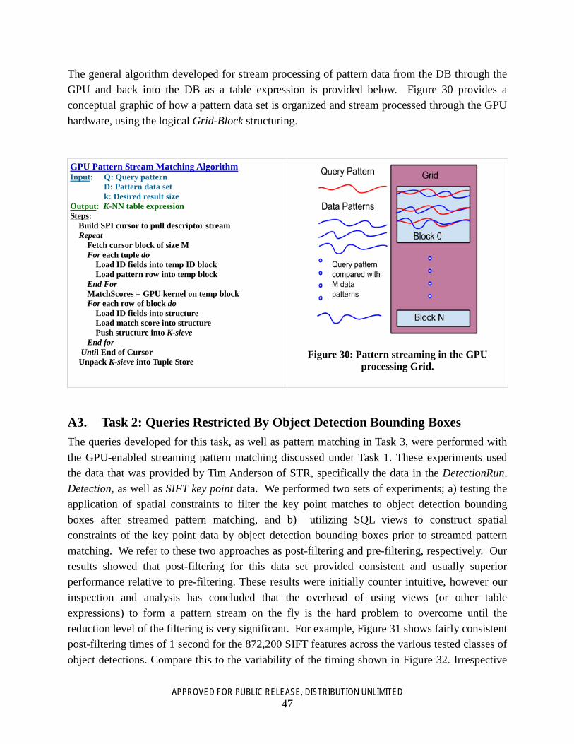
APPROVED FOR PUBLIC RELEASE, DISTRIBUTION UNLIMITED 47
The general algorithm developed for stream processing of pattern data from the DB through the GPU and back into the DB as a table expression is provided below. Figure 30 provides a conceptual graphic of how a pattern data set is organized and stream processed through the GPU hardware, using the logical Grid-Block structuring.
GPU Pattern Stream Matching Algorithm Input: Q: Query pattern D: Pattern data set k: Desired result size Output: K-NN table expression Steps: Build SPI cursor to pull descriptor stream Repeat Fetch cursor block of size M For each tuple do Load ID fields into temp ID block Load pattern row into temp block End For MatchScores = GPU kernel on temp block For each row of block do Load ID fields into structure Load match score into structure Push structure into K-sieve End for Until End of Cursor Unpack K-sieve into Tuple Store
Figure 30: Pattern streaming in the GPU processing Grid.
A3. Task 2: Queries Restricted By Object Detection Bounding Boxes The queries developed for this task, as well as pattern matching in Task 3, were performed with the GPU-enabled streaming pattern matching discussed under Task 1. These experiments used the data that was provided by Tim Anderson of STR, specifically the data in the DetectionRun, Detection, as well as SIFT key point data. We performed two sets of experiments; a) testing the application of spatial constraints to filter the key point matches to object detection bounding boxes after streamed pattern matching, and b) utilizing SQL views to construct spatial constraints of the key point data by object detection bounding boxes prior to streamed pattern matching. We refer to these two approaches as post-filtering and pre-filtering, respectively. Our results showed that post-filtering for this data set provided consistent and usually superior performance relative to pre-filtering. These results were initially counter intuitive, however our inspection and analysis has concluded that the overhead of using views (or other table expressions) to form a pattern stream on the fly is the hard problem to overcome until the reduction level of the filtering is very significant. For example, Figure 31 shows fairly consistent post-filtering times of 1 second for the 872,200 SIFT features across the various tested classes of object detections. Compare this to the variability of the timing shown in Figure 32. Irrespective

APPROVED FOR PUBLIC RELEASE, DISTRIBUTION UNLIMITED 48
of which spatial filtering method that is utilized, this work demonstrated conclusively that this design facilitates the integration of numerical feature vectors into a traditional database management system, thereby granting the affordances of well developed enterprise DBMS.
Table 2 provides the numerical counts of the various object detection bounding boxes for each class tested. The SOW specified vehicles and people, and we additionally tested the sub-class of vehicle, motorcycles. Additionally, the face detection class was available so that was tested as well.
Table 2: Object Detection Bounding Box Summary; counts, KPs, and performance.
A3.1 Post-filtered pattern matching The post-filtering of the output pattern matching stream via the spatial constraints of the object detection bounding boxes provided very consistent performance, irrespective of the number of object detections within the database. For our given SIFT feature set, the time is predominantly that of streaming the patterns through the GPU. Then, the output table expression is used in relational and spatial operations oriented towards filtering by bounding boxes of the detected object classes.
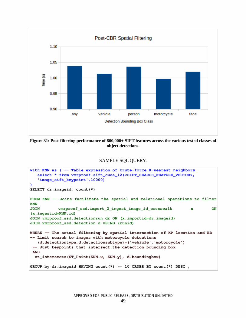
APPROVED FOR PUBLIC RELEASE, DISTRIBUTION UNLIMITED 49
Figure 31: Post-filtering performance of 800,000+ SIFT features across the various tested classes of object detections.
SAMPLE SQL QUERY:
with KNN as ( -- Table expression of brute-force K-nearest neighbors select * from vmrproof.sift_cuda_l2(<SIFT_SEARCH_FEATURE_VECTOR>, 'image_sift_keypoint',10000) ) SELECT dr.imageid, count(*) FROM KNN -- Joins facilitate the spatial and relational operations to filter KNN JOIN vmrproof_ssd.import_2_ingest_image_id_crosswalk x ON (x.ingestid=KNN.id) JOIN vmrproof_ssd.detectionrun dr ON (x.importid=dr.imageid) JOIN vmrproof_ssd.detection d USING (runid) WHERE -- The actual filtering by spatial intersection of KP location and BB -- Limit search to images with motorcycle detections (d.detectiontype,d.detectionsubtype)=('vehicle','motorcycle') -- Just keypoints that intersect the detection bounding box AND st_intersects(ST_Point(KNN.x, KNN.y), d.boundingbox) GROUP by dr.imageid HAVING count(*) >= 10 ORDER BY count(*) DESC ;

APPROVED FOR PUBLIC RELEASE, DISTRIBUTION UNLIMITED 50
A3.2 Pre-filtered pattern matching The pre-filtering of the input pattern stream via the spatial constraints of the object detection bounding boxes provided surprising results. Our initial hypothesis was that this would provide substantial acceleration versus brute force processing. However, this turned out to not be the case consistently. Instead, we have determined that the intermediate work the database does to stage the table expression (versus piping data directly from storage tables) is a substantial amount of overhead to overcome. As can be seen in Figure 32, the timing variability is highly influenced by the amount of stream reduction size; only showing improved search time relative to post-filtering for the motorcycle class.
A key discovery is the degree of which pre-filtering must reduce the search space to see benefits given the cost of the pre-filtering table expressions. For example, vehicle bounding box pre-filtered key point searches had a search space reduction of 94.6%, but saw an increased average search time of 0.35 seconds (roughly 35%). In contrast, the motorcycle bounding box pre-filtered key point searches reduced the search space by 99.6% and saw a massive reduction in search time by 0.94 seconds, a 94% acceleration. We believe there is an threshold of reduction that allows massive time efficiencies once the search space is significantly reduced. For our data set, we expect this value to be around 96%. Significantly broader scale experimentation is necessary to fully understand this characteristic of our design.

APPROVED FOR PUBLIC RELEASE, DISTRIBUTION UNLIMITED 51
Figure 32: Pre-filtering performance of 800,000+ SIFT features across the various tested classes of object detections.
SAMPLE SQL SPATIAL RESTRICTION VIEW & QUERY PRE-FILTERED KNN:
-- VIEW : Motorcycle Intersected keypoints CREATE OR REPLACE VIEW vmrproof_ssd.motorcycle_bounding_box_kp AS SELECT DISTINCT dr.imageid, ikp.keypoint, ikp.x, ikp.y, ikp.descriptor FROM vmrproof_ssd.detection d JOIN vmrproof_ssd.detectionrun dr USING (runid) JOIN vmrproof_ssd.import_2_ingest_image_id_crosswalk x ON x.importid = dr.imageid JOIN vmrproof_ssd.image_sift_keypoint ikp ON x.ingestid = ikp.imageid -- Just keypoints that intersect the detection bounding box of desired detection WHERE st_intersects(ST_Point( ikp.x, ikp.y), d.boundingbox) AND (d.detectiontype,d.detectionsubtype)=('vehicle','motorcycle'); -- QUERY : Search K-nearest neighbors, of pre-filtered data set select id,count(*) from vmrproof.sift_cuda_l2(<SIFT_SEARCH_FEATURE_VECTOR>, 'motorcycle_bounding_box_kp',10000) GROUP by id HAVING count(*) >= 10 ORDER BY count(*) DESC ;
A4. Task 3: Explore Performance Improvement Via Feature Indexing To explore the use of indexing techniques on the data we implemented a K-D tree partitioning scheme in the DB that partitioned the data set of SIFT key points into buckets of approximately 500 members. The K-D tree was induced using a data adaptive method, such that at every decision node the data bound within that node was analyzed to split along the feature dimension of greatest variance. Due to the secondary space constraints, these experiments had to be done in traditional storage not SSD. Therefore the times are roughly an order of magnitude higher than the equivalent sets of experiments.
Figure 33 shows the timing trends of our experiments using successively larger key point data sets ranging from 100,000 to 800,000. At the time these experiments were designed and started, we had not yet completed the timing and analysis of the Task 2 components. As such, the approach used relies heavily on the use of pre-constraining the data via table expressions that limit the searched data to a set of index leaves. We conducted our search experiments with a variety of result set sizes, requesting 500, 1000, 1500, 2000, and 2500 nearest neighbors. Our analysis shows little cost associated with retrieving the larger result set size, relative to the costs of performing the index search.
We expect that given a database of large enough size, and some refactoring of the index search code based on the insight from Task 2, we can achieve significant acceleration of this in the future.

APPROVED FOR PUBLIC RELEASE, DISTRIBUTION UNLIMITED 52
Figure 33: Performance analysis using a indexing scheme, pulling the 500, 1000, 1500, 2000, 2500-
nearest neighbors, plotted against increasing database sizes.
Table 3: Index CBR Search Times
Table 3 provides the summary data from our experiments with indexed retrieval. The brute-force timing on the data is provided for reference as the bottom row. We now understand that the constructed table expressions that link data to index leaves and produces the data stream on the fly based on leaf membership in the index will require substantially larger database size to leave size ratios to achieve notable improvements. Other techniques that may provide fruitful results may include hashing techniques, which then use post-filtering to expand from the hashed data back into full feature vectors. This is possible when the hashed values become the pattern database that is streamed through the GPU.

APPROVED FOR PUBLIC RELEASE, DISTRIBUTION UNLIMITED 53
A5. Conclusions
The use of relational database management system for numerical pattern data, whether it be key point or other types of patterns, is a viable option. However, careful consideration must be taken to evaluate access patterns regarding the use of table expressions within the database in accordance with the pattern matching capability. Traditional databases are well equipped to perform this analysis for relational data by utilizing table statistics and the built in query optimizer. We are not afforded this luxury, as we are adding very complex capabilities beyond the traditional use of an enterprise DBMS.

APPROVED FOR PUBLIC RELEASE, DISTRIBUTION UNLIMITED 54
LIST OF ACRONYMS
CUDA Compute Unified Device Architecture
DARPA Defense Advanced Research Projects Agency
DEM Digital Elevation Map
DSM Digital Surface Map
DTED Digital Topographical Elevation Data
GPU Graphics Processing Unit
GSD Ground Sample Distance
SRTM Shuttle Radar Topography Mission
VMR Visual Media Reasoning
DIG Database Indexing Group