visual motion many slides adapted from s. seitz, r. szeliski, m. pollefeys
Post on 21-Dec-2015
218 views
TRANSCRIPT
Visual motion
Many slides adapted from S. Seitz, R. Szeliski, M. Pollefeys
Outline
• Applications of segmentation to video• Motion and perceptual organization• Motion field• Optical flow• Motion segmentation with layers
Video
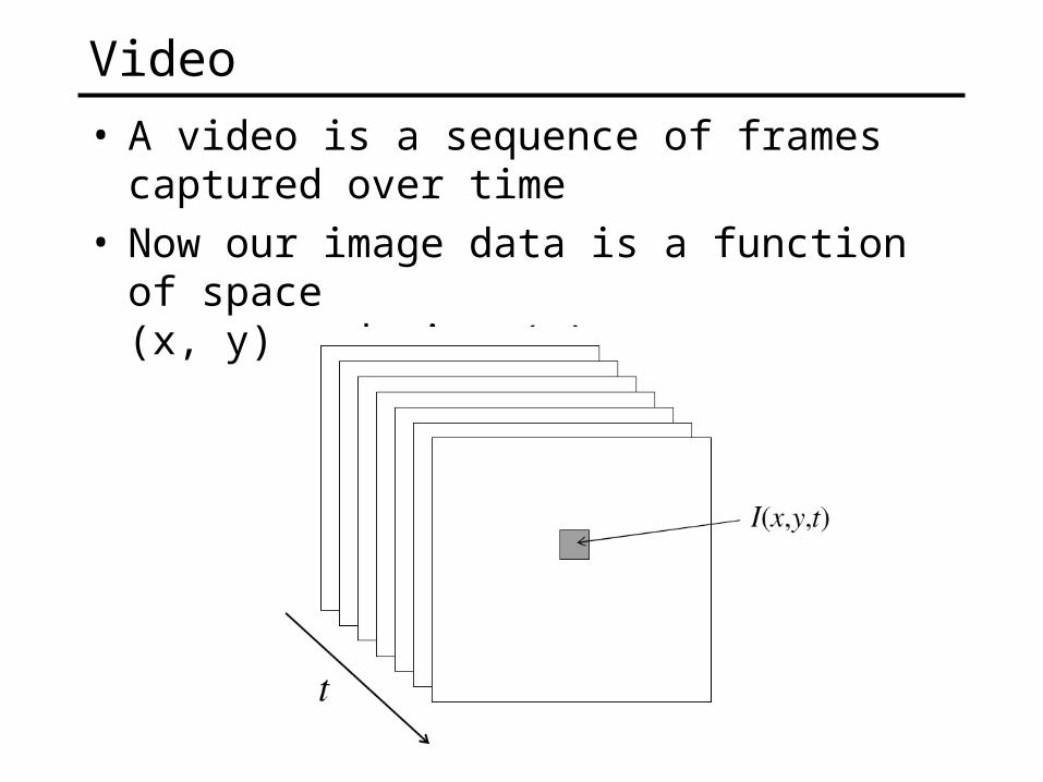
• A video is a sequence of frames captured over time
• Now our image data is a function of space (x, y) and time (t)
Applications of segmentation to video
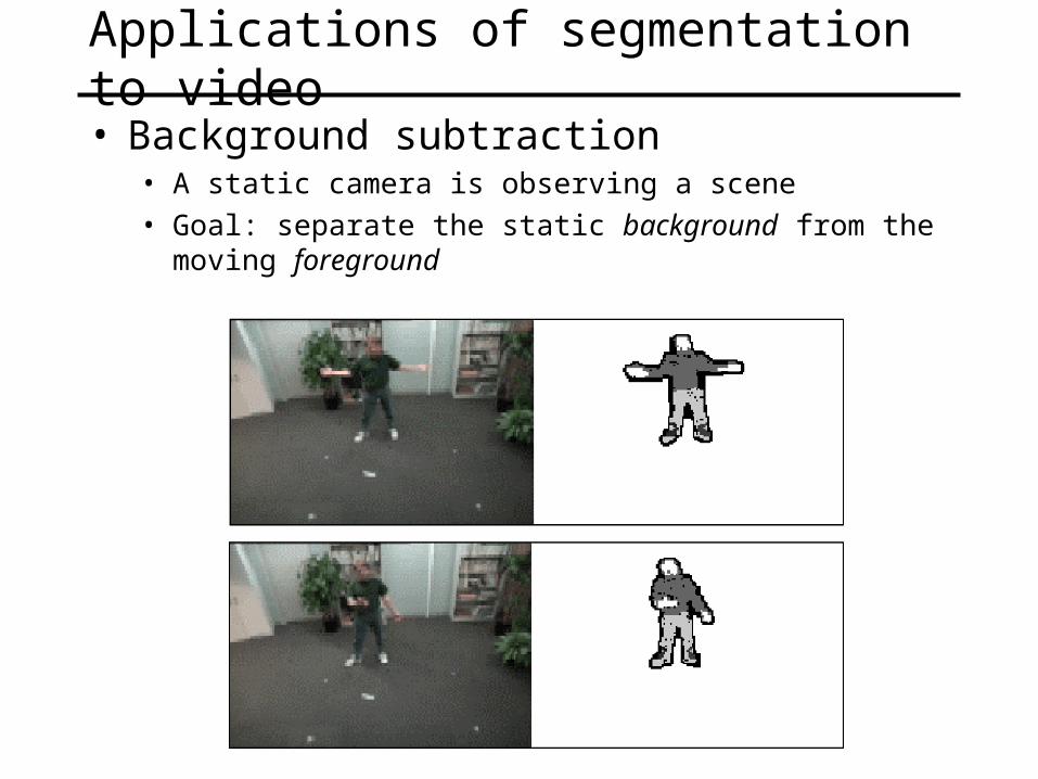
• Background subtraction• A static camera is observing a scene• Goal: separate the static background from the moving
foreground
Applications of segmentation to video
• Background subtraction• Form an initial background estimate• For each frame:
– Update estimate using a moving average
– Subtract the background estimate from the frame
– Label as foreground each pixel where the magnitude of the difference is greater than some threshold
– Use median filtering to “clean up” the results
Applications of segmentation to video
• Background subtraction• Shot boundary detection
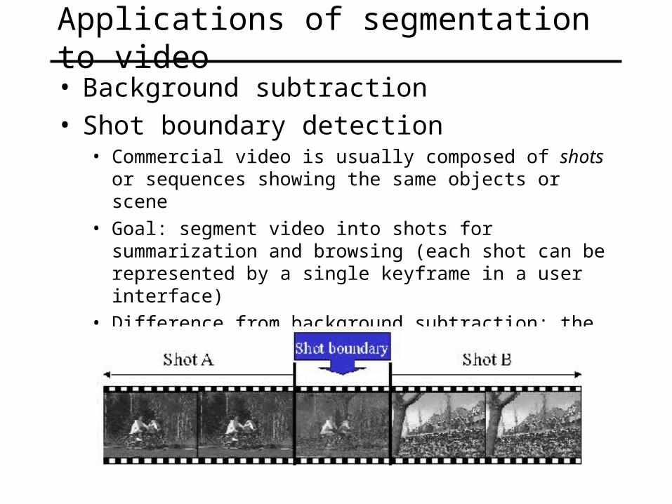
• Commercial video is usually composed of shots or sequences showing the same objects or scene
• Goal: segment video into shots for summarization and browsing (each shot can be represented by a single keyframe in a user interface)
• Difference from background subtraction: the camera is not necessarily stationary
Applications of segmentation to video
• Background subtraction• Shot boundary detection
• For each frame– Compute the distance between the current frame and the
previous one» Pixel-by-pixel differences» Differences of color histograms» Block comparison
– If the distance is greater than some threshold, classify the frame as a shot boundary
Applications of segmentation to video
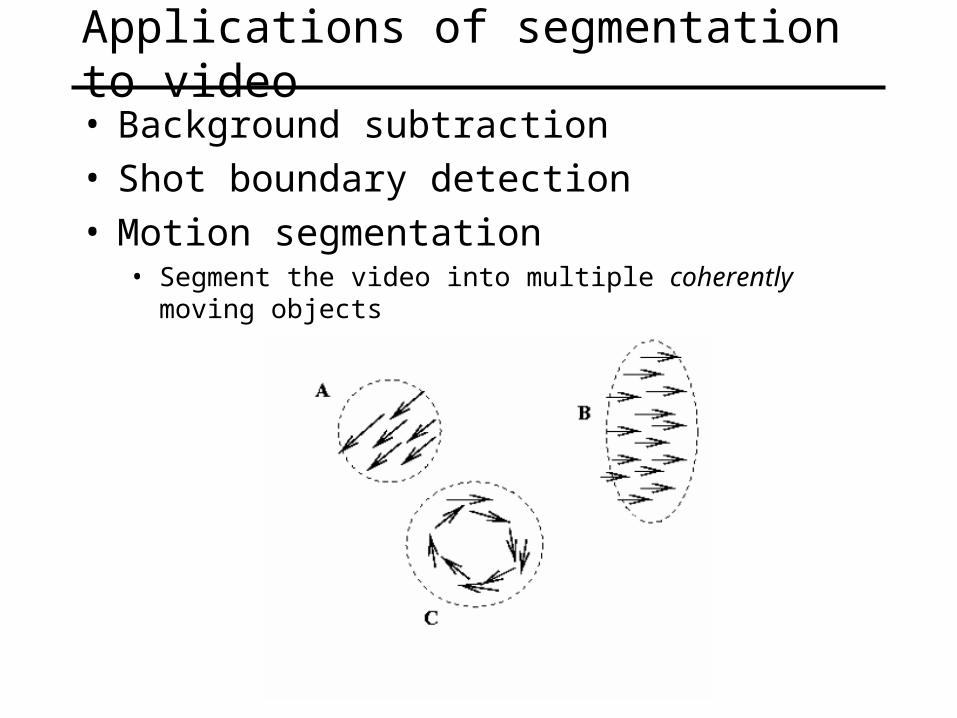
• Background subtraction• Shot boundary detection• Motion segmentation
• Segment the video into multiple coherently moving objects
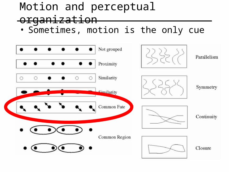
Motion and perceptual organization
• Sometimes, motion is the only cue
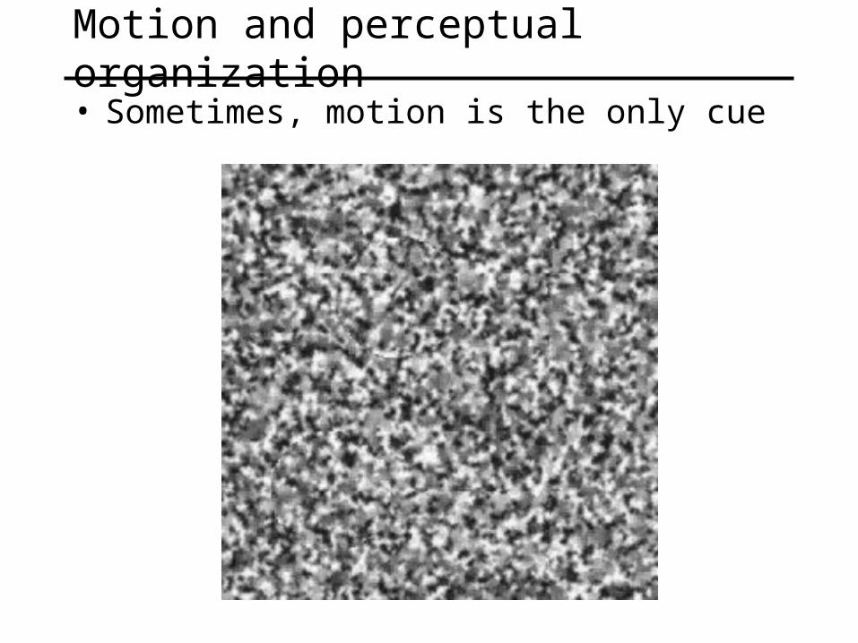
Motion and perceptual organization
• Sometimes, motion is the only cue

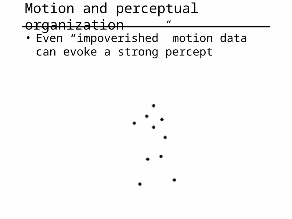
Motion and perceptual organization
• Even “impoverished” motion data can evoke a strong percept
Motion and perceptual organization
• Even “impoverished” motion data can evoke a strong percept
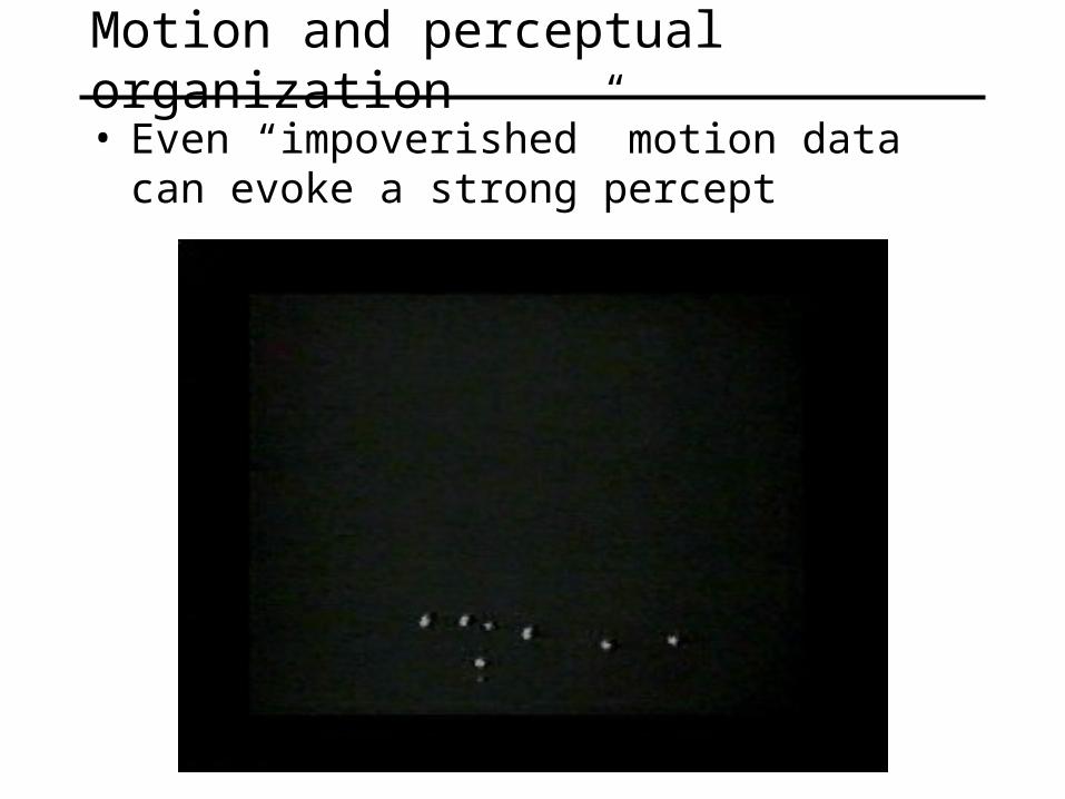
Motion and perceptual organization
• Even “impoverished” motion data can evoke a strong percept
Uses of motion
• Estimating 3D structure• Segmenting objects based on motion cues• Learning dynamical models• Recognizing events and activities• Improving video quality (motion stabilization)
Motion estimation techniques
• Direct methods• Directly recover image motion at each pixel from spatio-temporal
image brightness variations• Dense motion fields, but sensitive to appearance variations• Suitable for video and when image motion is small
• Feature-based methods• Extract visual features (corners, textured areas) and track them
over multiple frames• Sparse motion fields, but more robust tracking• Suitable when image motion is large (10s of pixels)
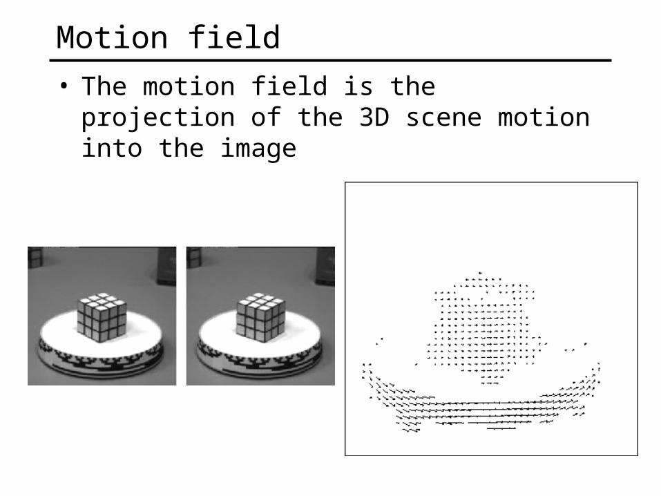
Motion field
• The motion field is the projection of the 3D scene motion into the image
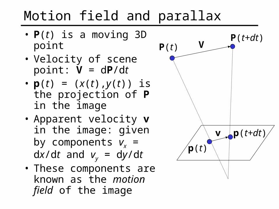
Motion field and parallax• P(t) is a moving 3D point• Velocity of scene point:
V = dP/dt• p(t) = (x(t),y(t)) is the
projection of P in the image
• Apparent velocity v in the image: given by components vx = dx/dt and vy = dy/dt
• These components are known as the motion field of the image
p(t)
p(t+dt)
P(t)P(t+dt)
V
v
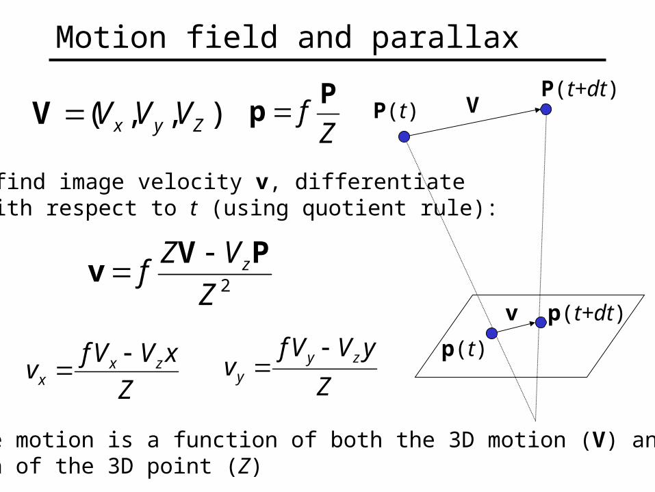
Motion field and parallax
p(t)
p(t+dt)
P(t)P(t+dt)
V
v
),,( Zyx VVVV
2Z
VZf zPV
v
Zf
Pp
To find image velocity v, differentiate p with respect to t (using quotient rule):
Z
xVVfv zxx
Z
yVVfv zyy
Image motion is a function of both the 3D motion (V) and thedepth of the 3D point (Z)
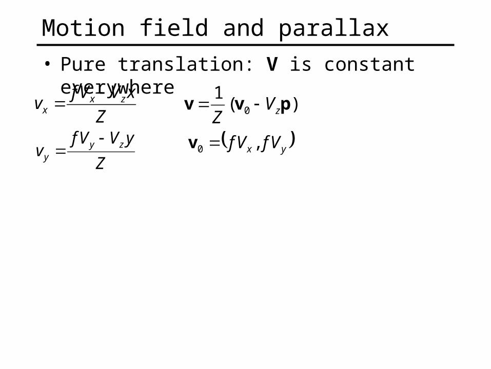
Motion field and parallax
• Pure translation: V is constant everywhere
Z
xVVfv zxx
Z
yVVfv zyy
),(1
0 pvv zVZ
yx VfVf ,0 v
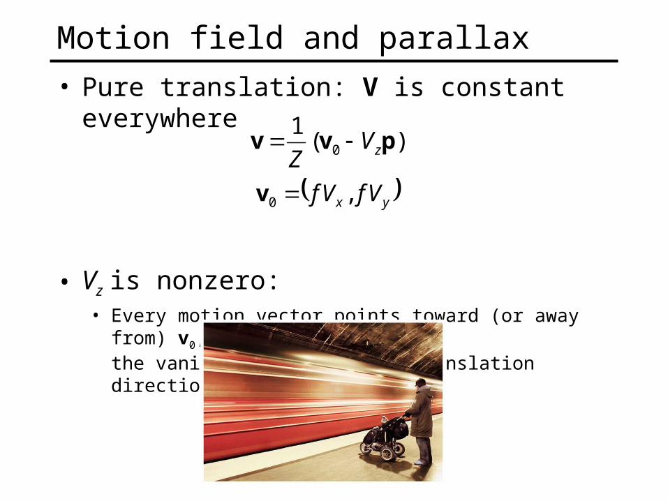
Motion field and parallax
• Pure translation: V is constant everywhere
• Vz is nonzero: • Every motion vector points toward (or away from) v0,
the vanishing point of the translation direction
),(1
0 pvv zVZ
yx VfVf ,0 v

Motion field and parallax
• Pure translation: V is constant everywhere
• Vz is nonzero: • Every motion vector points toward (or away from) v0,
the vanishing point of the translation direction
• Vz is zero: • Motion is parallel to the image plane, all the motion vectors are
parallel
• The length of the motion vectors is inversely proportional to the depth Z
),(1
0 pvv zVZ
yx VfVf ,0 v
Optical flow
• Definition: optical flow is the apparent motion of brightness patterns in the image
• Ideally, optical flow would be the same as the motion field
• Have to be careful: apparent motion can be caused by lighting changes without any actual motion• Think of a uniform rotating sphere under fixed lighting vs. a
stationary sphere under moving illumination
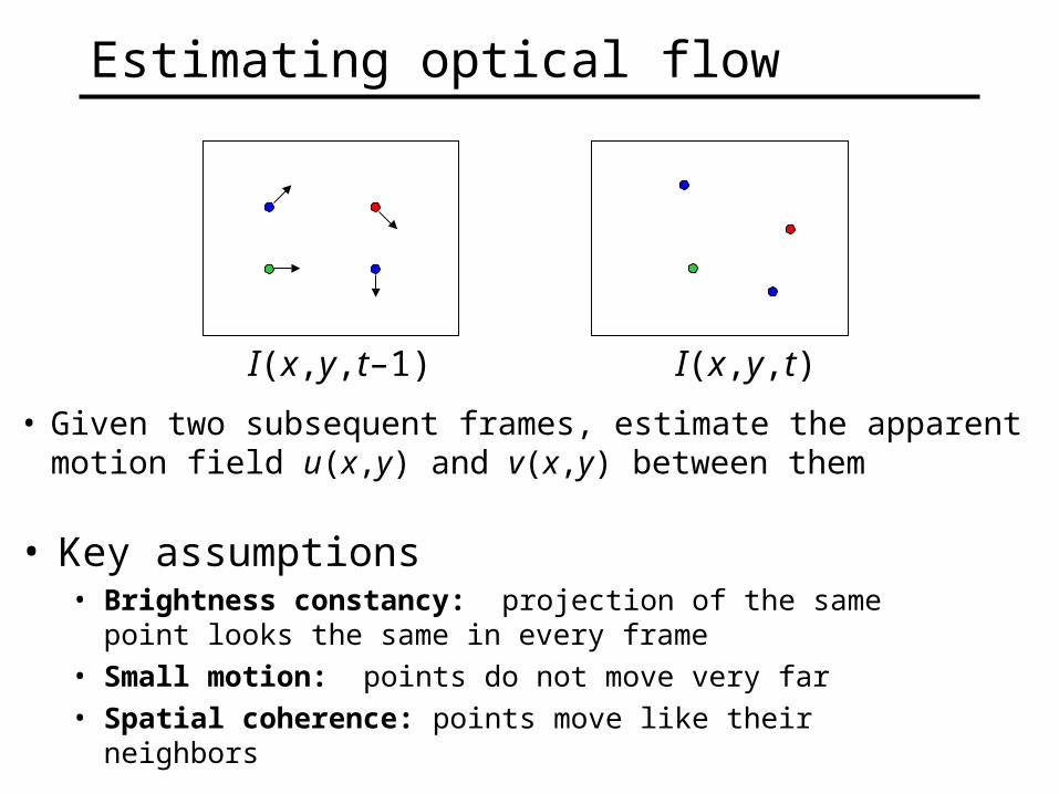
Estimating optical flow
• Given two subsequent frames, estimate the apparent motion field u(x,y) and v(x,y) between them
• Key assumptions• Brightness constancy: projection of the same point looks the
same in every frame• Small motion: points do not move very far• Spatial coherence: points move like their neighbors
I(x,y,t–1) I(x,y,t)
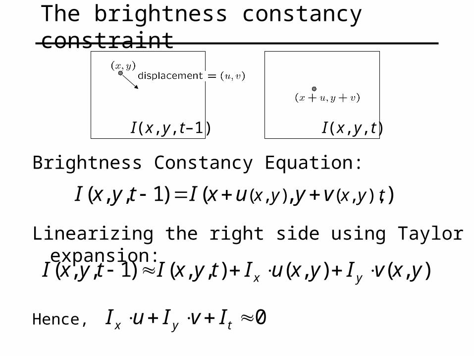
Brightness Constancy Equation:
),()1,,( ),,(),( tyxyx vyuxItyxI
),(),(),,()1,,( yxvIyxuItyxItyxI yx
Linearizing the right side using Taylor expansion:
The brightness constancy constraint
I(x,y,t–1) I(x,y,t)
0 tyx IvIuIHence,
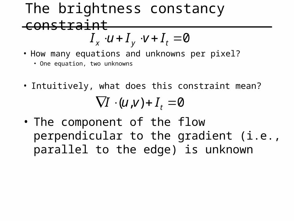
The brightness constancy constraint
• How many equations and unknowns per pixel?• One equation, two unknowns
• Intuitively, what does this constraint mean?
• The component of the flow perpendicular to the gradient (i.e., parallel to the edge) is unknown
0 tyx IvIuI
0),( tIvuI
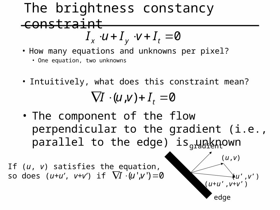
The brightness constancy constraint
• How many equations and unknowns per pixel?• One equation, two unknowns
• Intuitively, what does this constraint mean?
• The component of the flow perpendicular to the gradient (i.e., parallel to the edge) is unknown
0 tyx IvIuI
0)','( vuI
edge
(u,v)
(u’,v’)
gradient
(u+u’,v+v’)
If (u, v) satisfies the equation, so does (u+u’, v+v’) if
0),( tIvuI
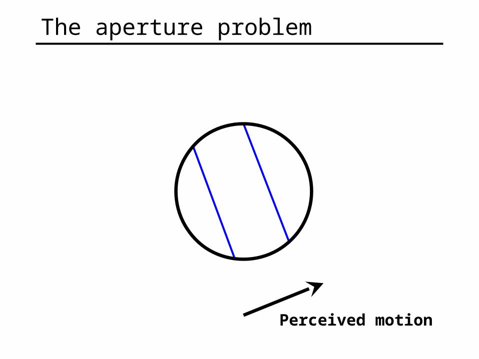
The aperture problem
Perceived motion

The aperture problem
Actual motion
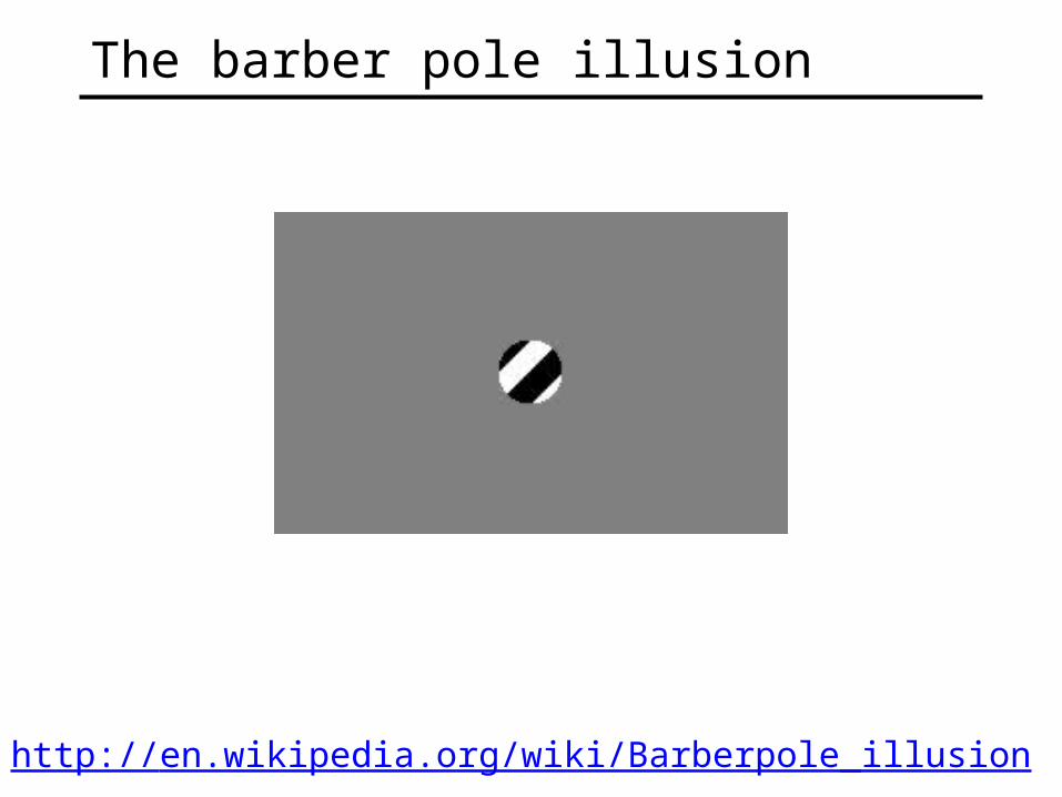
The barber pole illusion
http://en.wikipedia.org/wiki/Barberpole_illusion
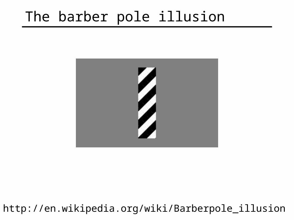
The barber pole illusion
http://en.wikipedia.org/wiki/Barberpole_illusion

The barber pole illusion
http://en.wikipedia.org/wiki/Barberpole_illusion
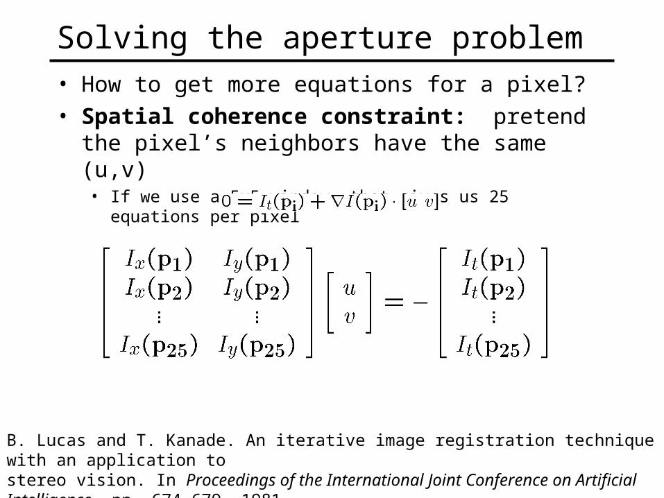
Solving the aperture problem• How to get more equations for a pixel?• Spatial coherence constraint: pretend the pixel’s
neighbors have the same (u,v)• If we use a 5x5 window, that gives us 25 equations per pixel
B. Lucas and T. Kanade. An iterative image registration technique with an application tostereo vision. In Proceedings of the International Joint Conference on Artificial Intelligence, pp. 674–679, 1981.

Solving the aperture problem• Least squares problem:
B. Lucas and T. Kanade. An iterative image registration technique with an application tostereo vision. In Proceedings of the International Joint Conference on Artificial Intelligence, pp. 674–679, 1981.
• When is this system solvable?• What if the window contains just a single straight edge?
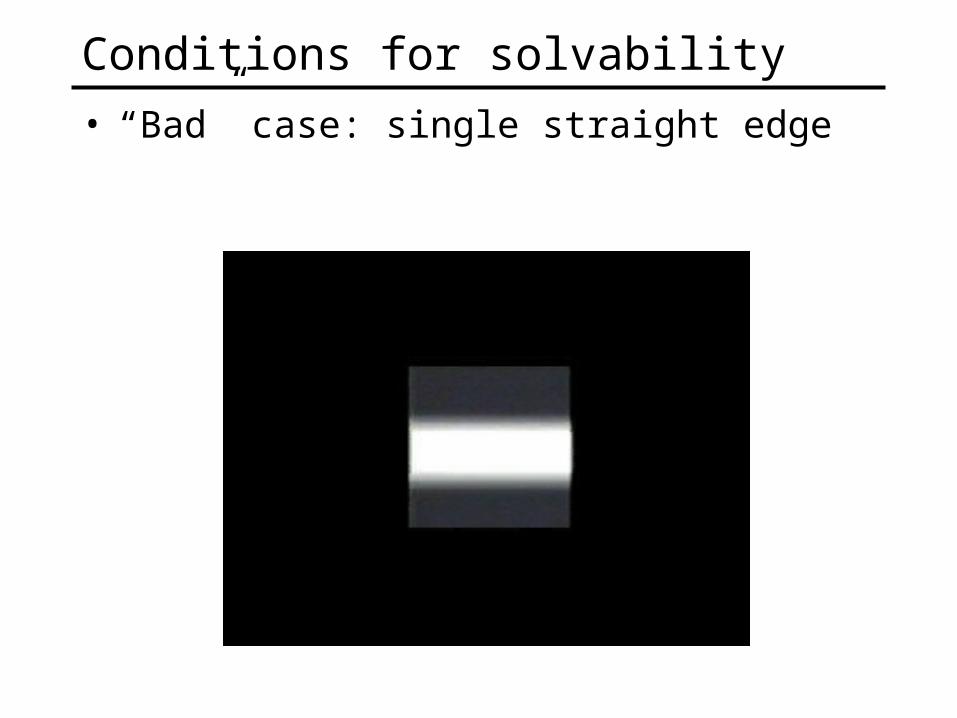
Conditions for solvability
• “Bad” case: single straight edge
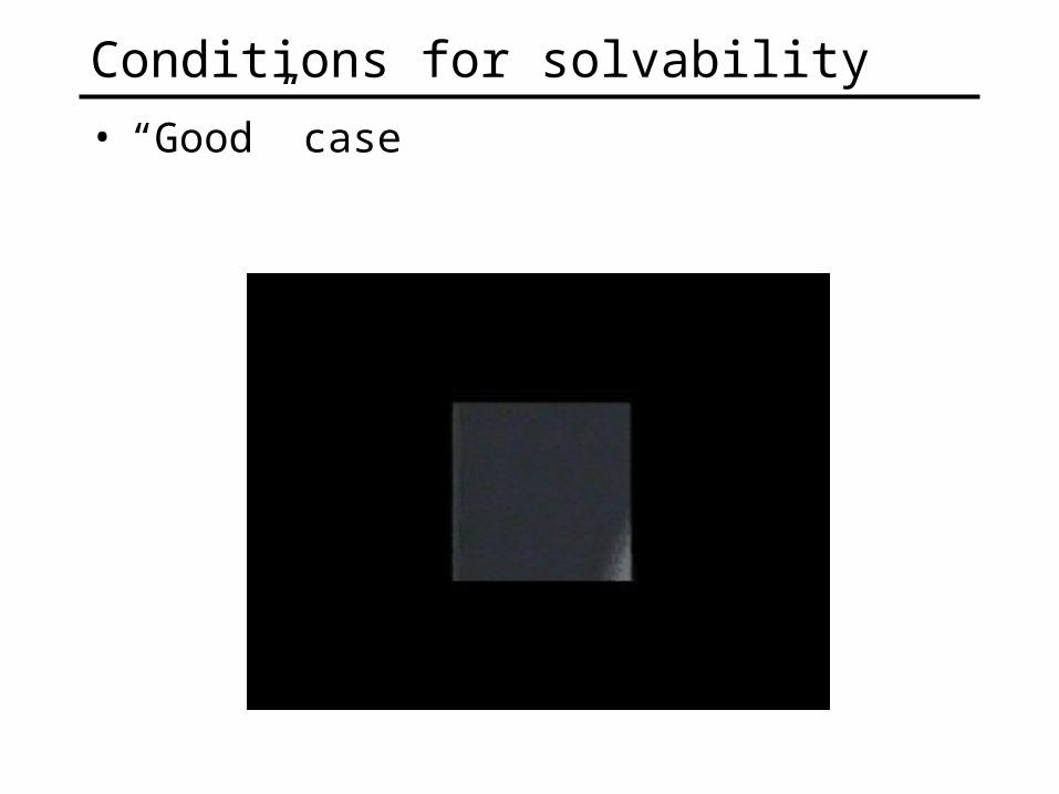
Conditions for solvability
• “Good” case
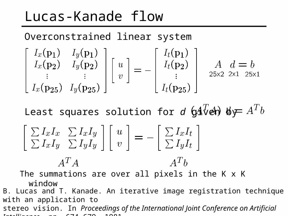
Lucas-Kanade flowOverconstrained linear system
B. Lucas and T. Kanade. An iterative image registration technique with an application tostereo vision. In Proceedings of the International Joint Conference on Artificial Intelligence, pp. 674–679, 1981.
The summations are over all pixels in the K x K window
Least squares solution for d given by
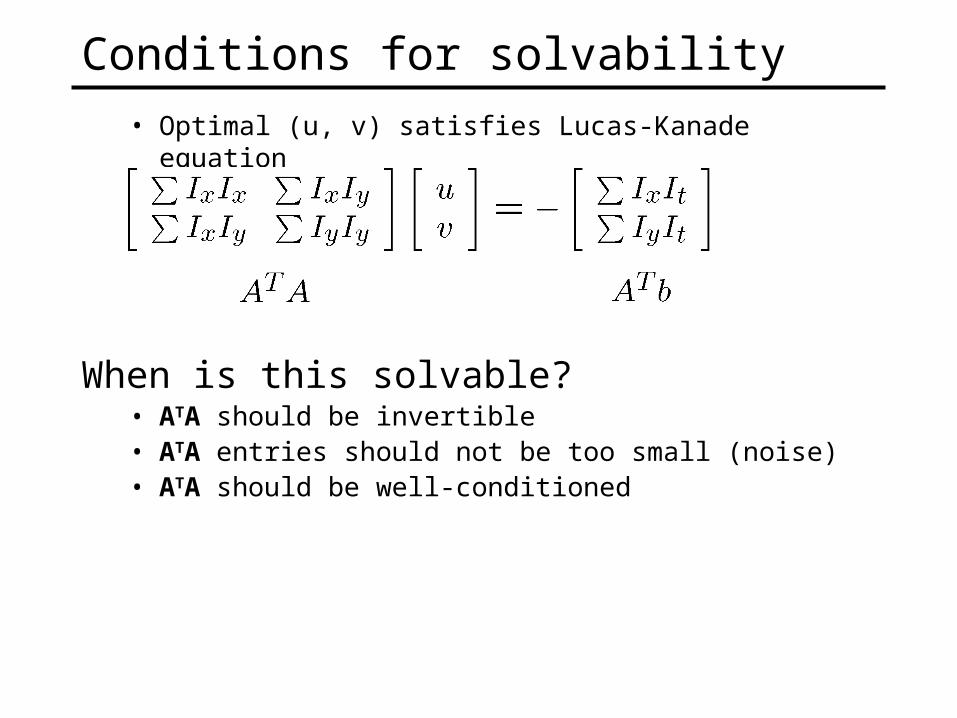
Conditions for solvability
• Optimal (u, v) satisfies Lucas-Kanade equation
When is this solvable?• ATA should be invertible • ATA entries should not be too small (noise)• ATA should be well-conditioned
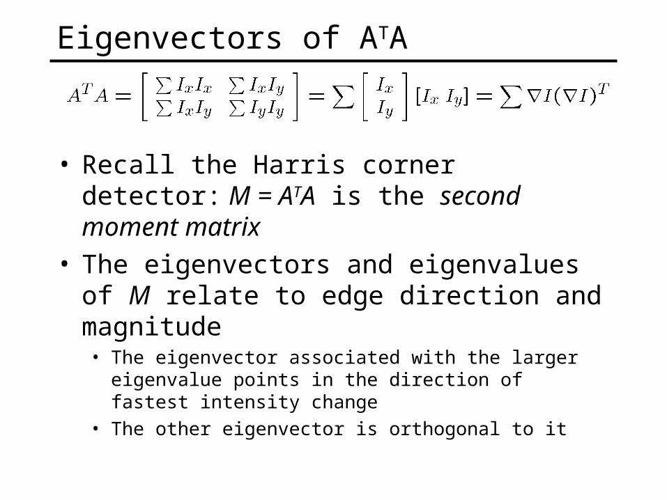
Eigenvectors of ATA
• Recall the Harris corner detector: M = ATA is the second moment matrix
• The eigenvectors and eigenvalues of M relate to edge direction and magnitude • The eigenvector associated with the larger eigenvalue points
in the direction of fastest intensity change• The other eigenvector is orthogonal to it
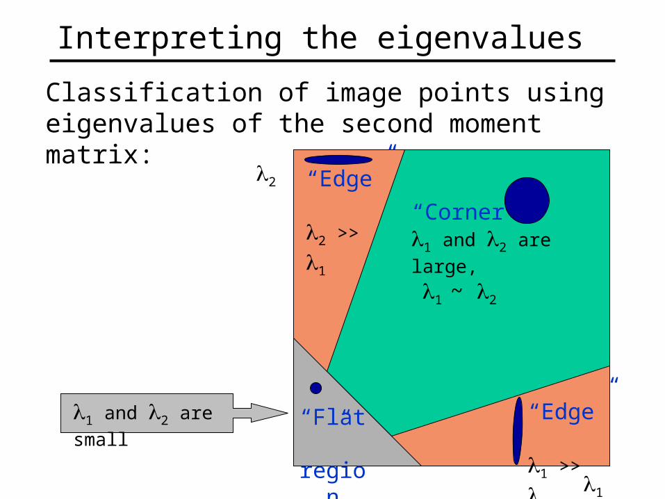
Interpreting the eigenvalues
1
2
“Corner”1 and 2 are large,
1 ~ 2
1 and 2 are small “Edge” 1 >> 2
“Edge” 2 >> 1
“Flat” region
Classification of image points using eigenvalues of the second moment matrix:

Edge
– gradients very large or very small– large1, small 2
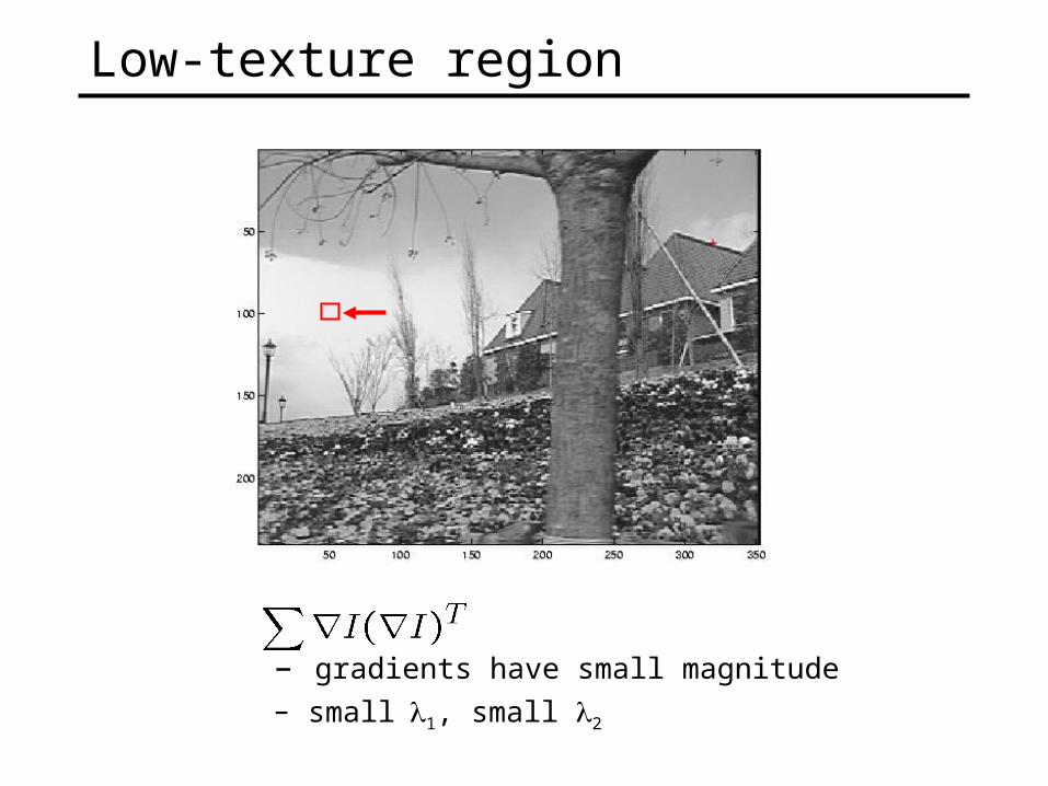
Low-texture region
– gradients have small magnitude
– small1, small 2

High-texture region
– gradients are different, large magnitudes
– large1, large 2
What are good features to track?
• Recall the Harris corner detector• Can measure “quality” of features from just a
single image
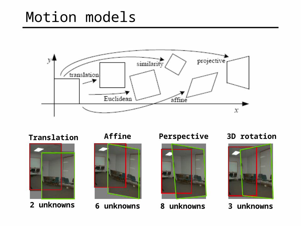
Motion models
Translation
2 unknowns
Affine
6 unknowns
Perspective
8 unknowns
3D rotation
3 unknowns
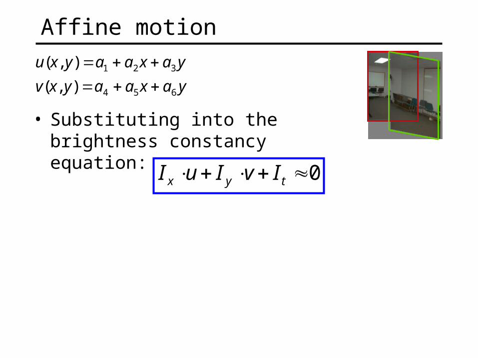
• Substituting into the brightness constancy equation:
yaxaayxv
yaxaayxu
654
321
),(
),(
0 tyx IvIuI
Affine motion
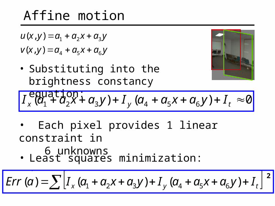
0)()( 654321 tyx IyaxaaIyaxaaI
• Substituting into the brightness constancy equation:
yaxaayxv
yaxaayxu
654
321
),(
),(
• Each pixel provides 1 linear constraint in 6 unknowns
2 tyx IyaxaaIyaxaaIaErr )()()( 654321
• Least squares minimization:
Affine motion
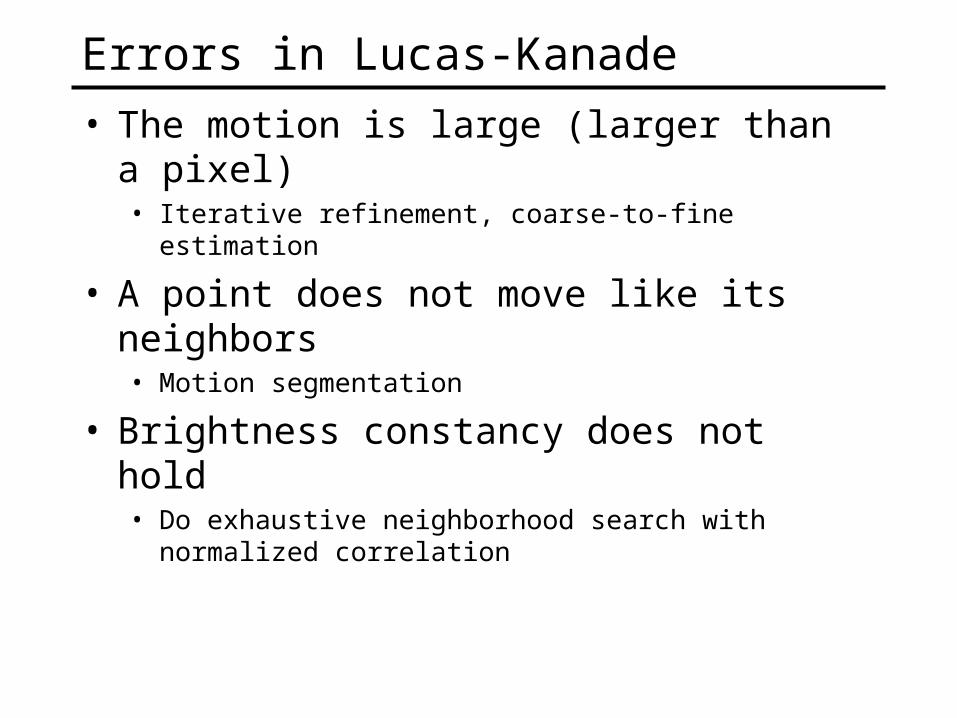
Errors in Lucas-Kanade
• The motion is large (larger than a pixel)• Iterative refinement, coarse-to-fine estimation
• A point does not move like its neighbors• Motion segmentation
• Brightness constancy does not hold• Do exhaustive neighborhood search with normalized
correlation
Iterative Refinement
• Estimate velocity at each pixel using one iteration of Lucas and Kanade estimation
• Warp one image toward the other using the estimated flow field
• Refine estimate by repeating the process
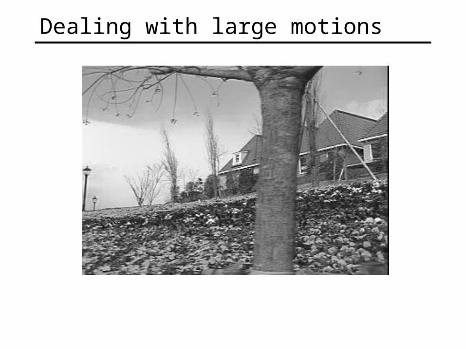
Dealing with large motions
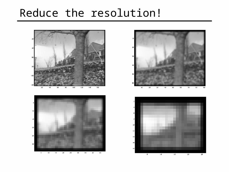
Reduce the resolution!
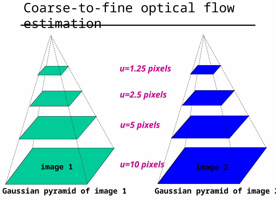
image Iimage H
Gaussian pyramid of image 1 Gaussian pyramid of image 2
image 2image 1 u=10 pixels
u=5 pixels
u=2.5 pixels
u=1.25 pixels
Coarse-to-fine optical flow estimation
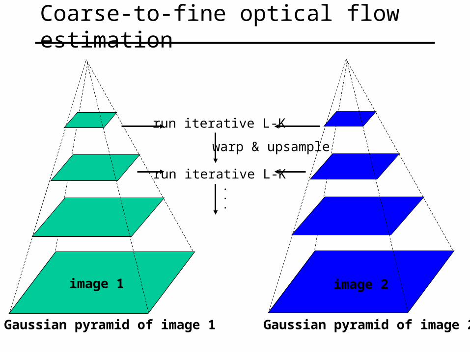
image Iimage J
Gaussian pyramid of image 1 Gaussian pyramid of image 2
image 2image 1
Coarse-to-fine optical flow estimation
run iterative L-K
run iterative L-K
warp & upsample
.
.
.
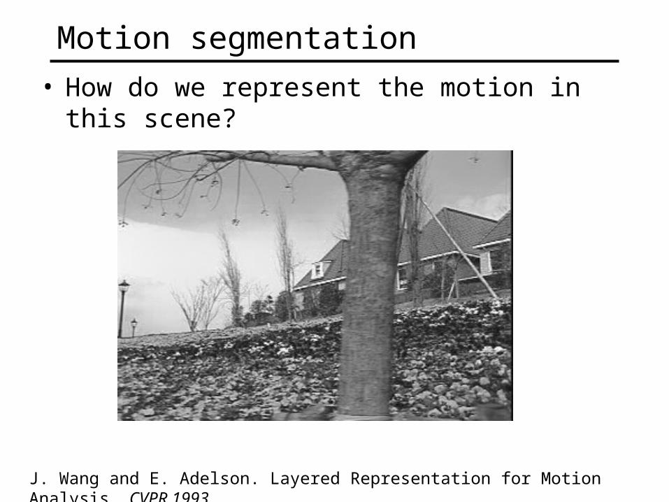
Motion segmentation
• How do we represent the motion in this scene?
J. Wang and E. Adelson. Layered Representation for Motion Analysis. CVPR 1993.
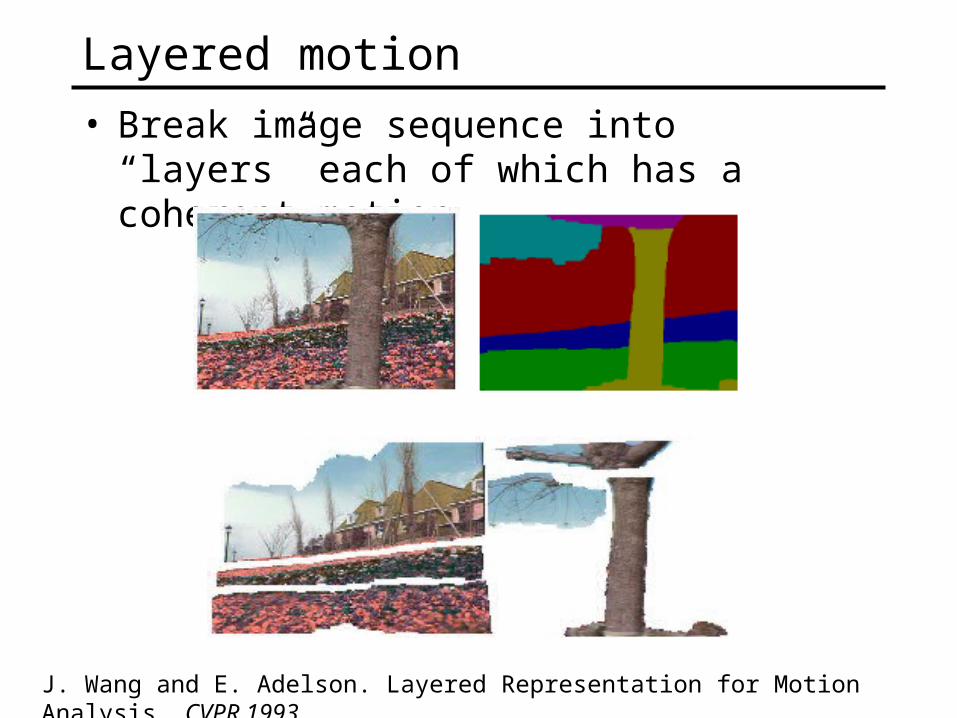
Layered motion
• Break image sequence into “layers” each of which has a coherent motion
J. Wang and E. Adelson. Layered Representation for Motion Analysis. CVPR 1993.
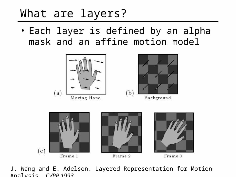
What are layers?
• Each layer is defined by an alpha mask and an affine motion model
J. Wang and E. Adelson. Layered Representation for Motion Analysis. CVPR 1993.
yaxaayxv
yaxaayxu
654
321
),(
),(
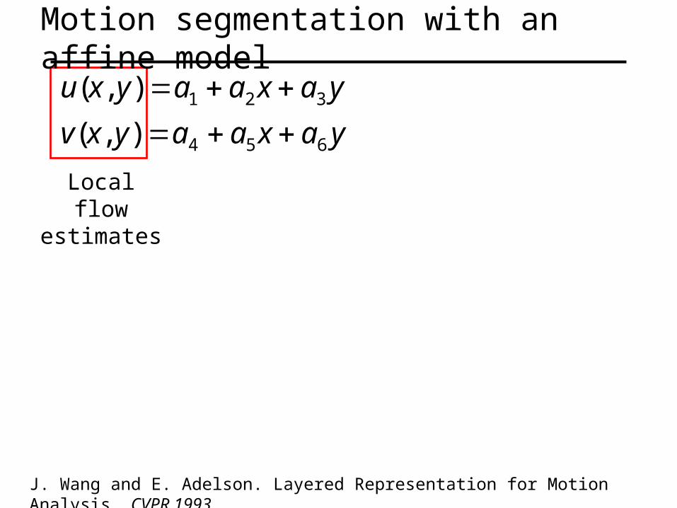
Local flow estimates
Motion segmentation with an affine model
J. Wang and E. Adelson. Layered Representation for Motion Analysis. CVPR 1993.
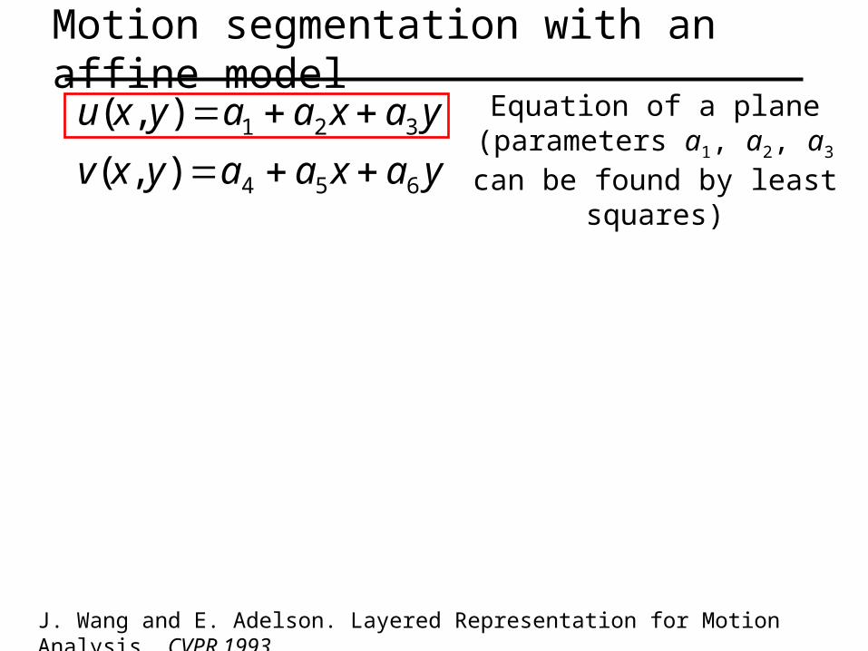
Motion segmentation with an affine model
yaxaayxv
yaxaayxu
654
321
),(
),(
Equation of a plane
(parameters a1, a2, a3 can be found by least squares)
J. Wang and E. Adelson. Layered Representation for Motion Analysis. CVPR 1993.
Motion segmentation with an affine model
yaxaayxv
yaxaayxu
654
321
),(
),(
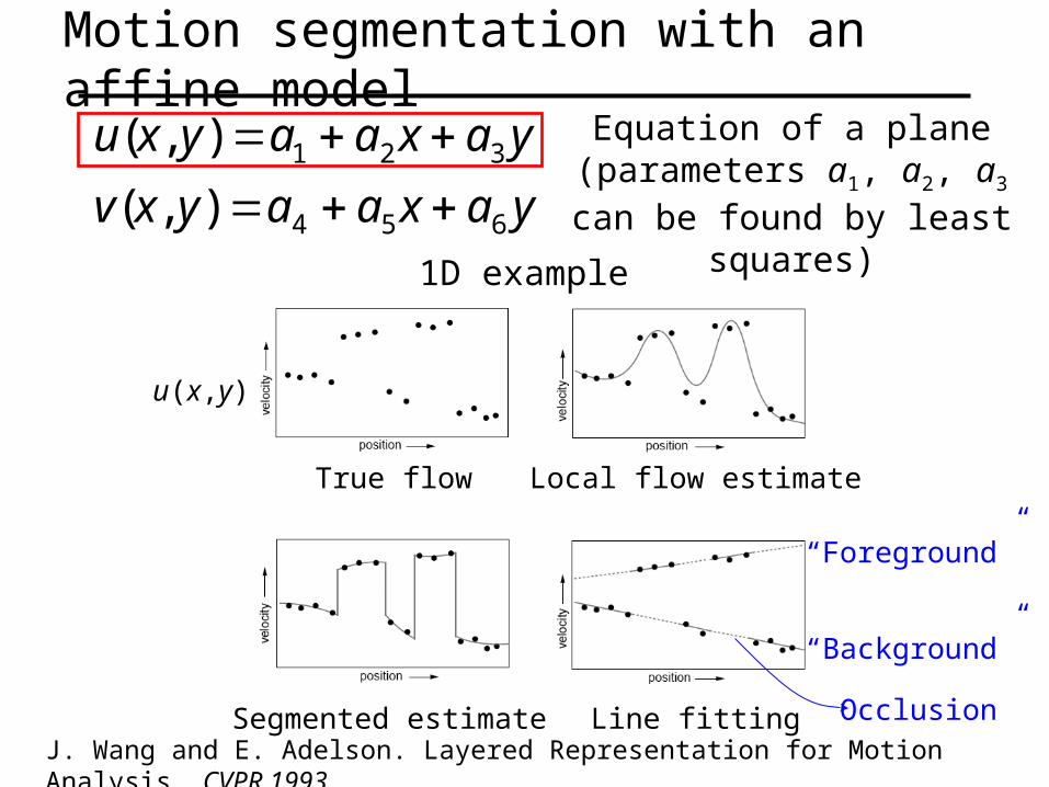
1D example
u(x,y)
Local flow estimate
Segmented estimate Line fitting
Equation of a plane(parameters a1, a2, a3 can be
found by least squares)
True flow
“Foreground”
“Background”
Occlusion
J. Wang and E. Adelson. Layered Representation for Motion Analysis. CVPR 1993.
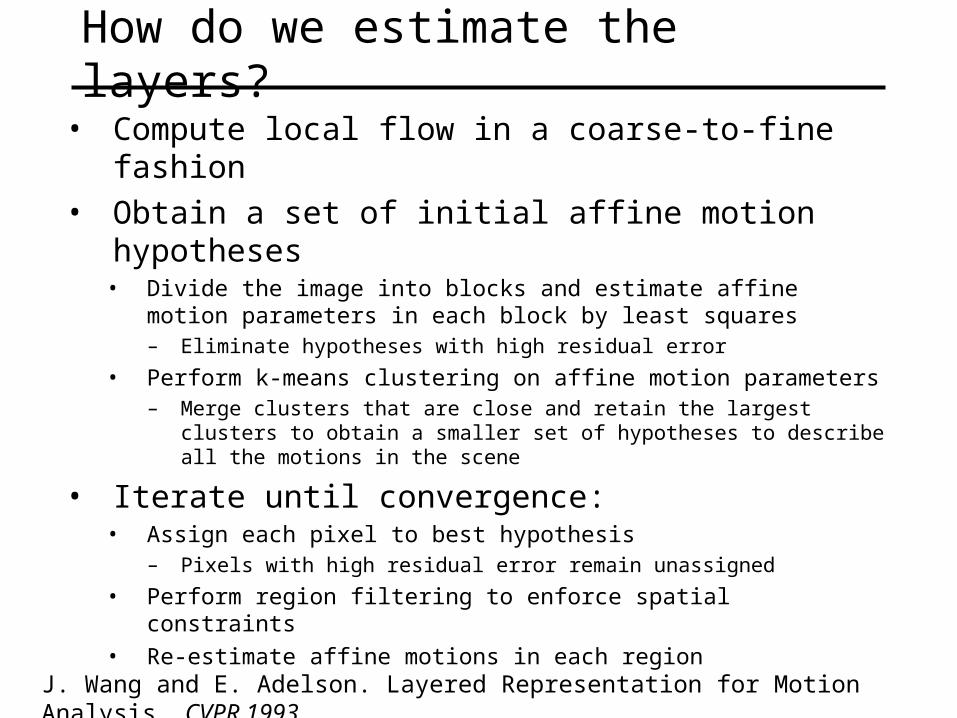
How do we estimate the layers?
• Compute local flow in a coarse-to-fine fashion• Obtain a set of initial affine motion hypotheses
• Divide the image into blocks and estimate affine motion parameters in each block by least squares– Eliminate hypotheses with high residual error
• Perform k-means clustering on affine motion parameters– Merge clusters that are close and retain the largest clusters to
obtain a smaller set of hypotheses to describe all the motions in the scene
• Iterate until convergence:• Assign each pixel to best hypothesis
– Pixels with high residual error remain unassigned
• Perform region filtering to enforce spatial constraints• Re-estimate affine motions in each region
J. Wang and E. Adelson. Layered Representation for Motion Analysis. CVPR 1993.
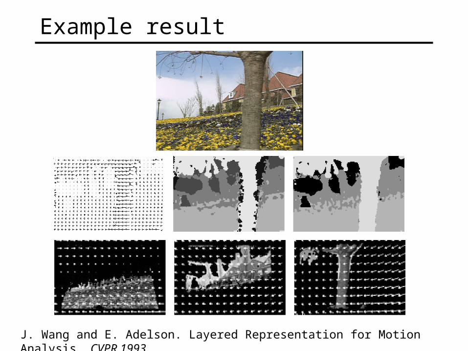
Example result
J. Wang and E. Adelson. Layered Representation for Motion Analysis. CVPR 1993.