VISUAL NEURAL SIMULATOR

Tutorial for the Receptive Fields Module

Copyright: Dr. Dario Ringach, 2015-02-24 Editors: Natalie Schottler & Dr. William Grisham

2

page 2 of 36

3

page 3 of 36

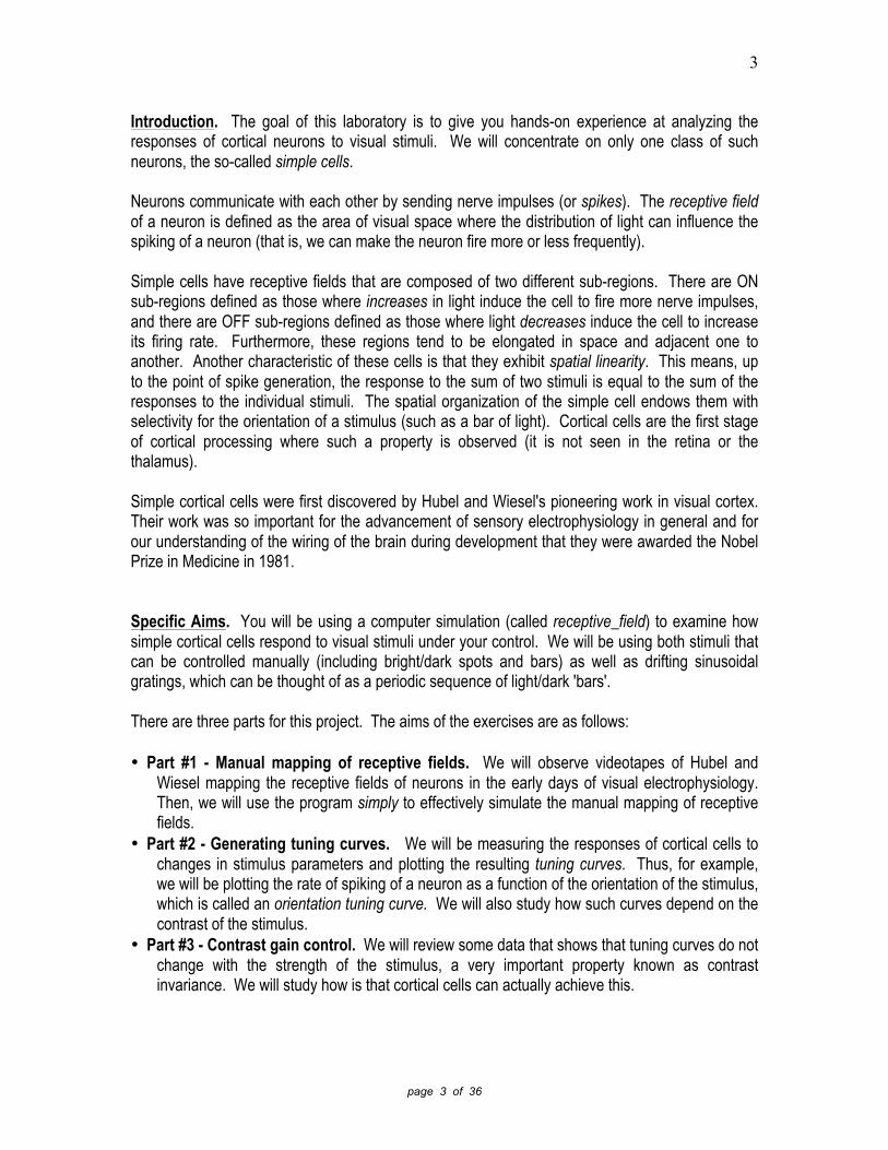
Introduction. The goal of this laboratory is to give you hands-on experience at analyzing the responses of cortical neurons to visual stimuli. We will concentrate on only one class of such neurons, the so-called simple cells. Neurons communicate with each other by sending nerve impulses (or spikes). The receptive field of a neuron is defined as the area of visual space where the distribution of light can influence the spiking of a neuron (that is, we can make the neuron fire more or less frequently). Simple cells have receptive fields that are composed of two different sub-regions. There are ON sub-regions defined as those where increases in light induce the cell to fire more nerve impulses, and there are OFF sub-regions defined as those where light decreases induce the cell to increase its firing rate. Furthermore, these regions tend to be elongated in space and adjacent one to another. Another characteristic of these cells is that they exhibit spatial linearity. This means, up to the point of spike generation, the response to the sum of two stimuli is equal to the sum of the responses to the individual stimuli. The spatial organization of the simple cell endows them with selectivity for the orientation of a stimulus (such as a bar of light). Cortical cells are the first stage of cortical processing where such a property is observed (it is not seen in the retina or the thalamus). Simple cortical cells were first discovered by Hubel and Wiesel's pioneering work in visual cortex. Their work was so important for the advancement of sensory electrophysiology in general and for our understanding of the wiring of the brain during development that they were awarded the Nobel Prize in Medicine in 1981. Specific Aims. You will be using a computer simulation (called receptive_field) to examine how simple cortical cells respond to visual stimuli under your control. We will be using both stimuli that can be controlled manually (including bright/dark spots and bars) as well as drifting sinusoidal gratings, which can be thought of as a periodic sequence of light/dark 'bars'. There are three parts for this project. The aims of the exercises are as follows: • Part #1 - Manual mapping of receptive fields. We will observe videotapes of Hubel and

Wiesel mapping the receptive fields of neurons in the early days of visual electrophysiology. Then, we will use the program simply to effectively simulate the manual mapping of receptive fields.

• Part #2 - Generating tuning curves. We will be measuring the responses of cortical cells to changes in stimulus parameters and plotting the resulting tuning curves. Thus, for example, we will be plotting the rate of spiking of a neuron as a function of the orientation of the stimulus, which is called an orientation tuning curve. We will also study how such curves depend on the contrast of the stimulus.

• Part #3 - Contrast gain control. We will review some data that shows that tuning curves do not change with the strength of the stimulus, a very important property known as contrast invariance. We will study how is that cortical cells can actually achieve this.

4

page 4 of 36

Part #1. To get stated, run Matlab by double-clicking the MATLAB R2007b shortcut on the desktop. A MATLAB 7.5.0 (R2007b) window will appear. In the Command Window section, type the following highlighted commands at the prompt (>>), hitting Return on the keyboard after each command. [Note: If you are using a digital copy of this tutorial, you may also copy the highlighted portions and paste them into the Command Window prompt.] cd receptive_field receptive_field_lab(1)

FIGURE 1 A receptive_field window will appear. You can now minimize the main MATLAB window since you will be only interacting with the receptive_field one. Click the Run button to initiate the simulation.

FIGURE 2

There are two images shown side by side in this interface. The Receptive Field image on the right shows the spatial organization of the receptive field of a simple cortical neuron. Here, areas in red hues indicate ON sub-regions while areas in blue hues indicate OFF sub-regions. Green regions are neutral (that is, they do not respond to light increases or decreases) and, therefore, are outside the receptive field of the cell. The Stimulus image on the left shows a visual stimulus region on the exact area of the visual field as the receptive field is on the right side of the window. Think of this window as a 'projection screen' where you will be projecting patterns of light, as spots or bars, which can be either lighter or darker than the gray background. These patterns of light will appear by moving the mouse within the visual stimulus region (gray box).

5

page 5 of 36

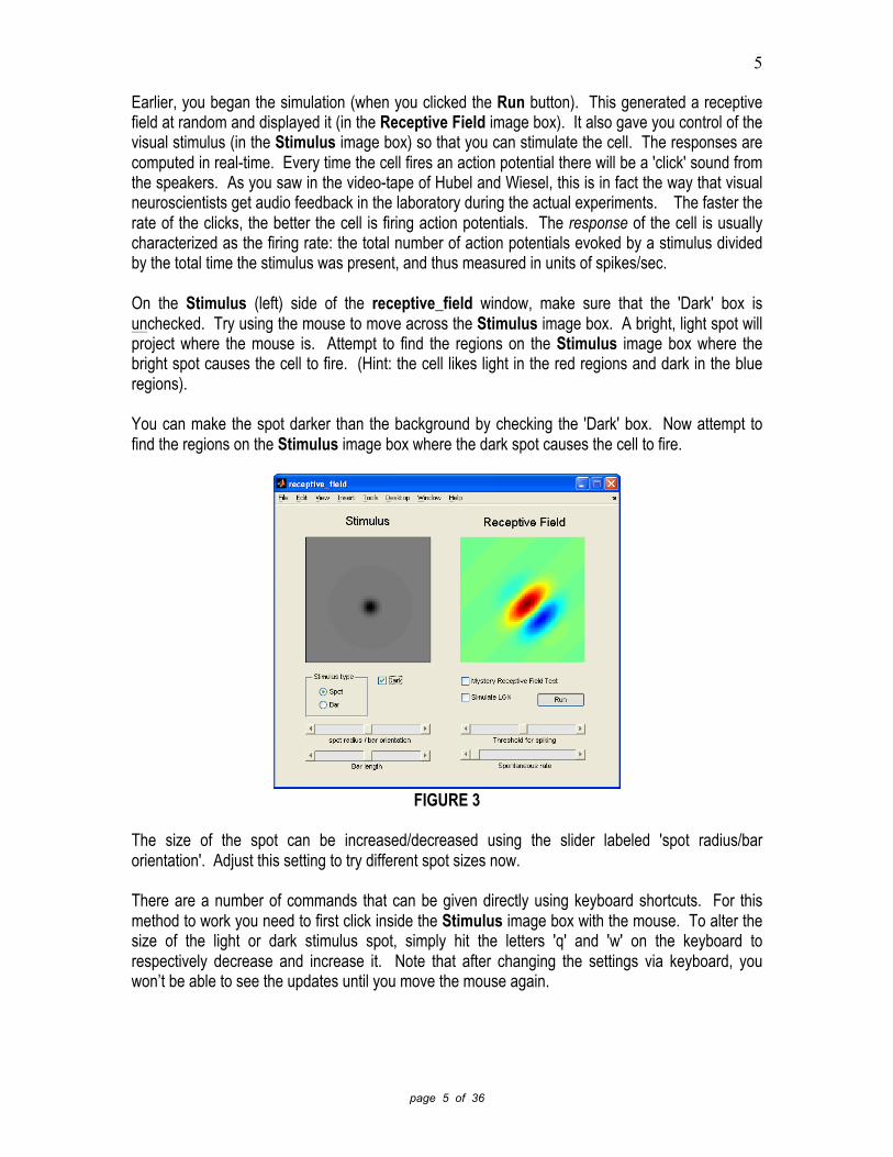
Earlier, you began the simulation (when you clicked the Run button). This generated a receptive field at random and displayed it (in the Receptive Field image box). It also gave you control of the visual stimulus (in the Stimulus image box) so that you can stimulate the cell. The responses are computed in real-time. Every time the cell fires an action potential there will be a 'click' sound from the speakers. As you saw in the video-tape of Hubel and Wiesel, this is in fact the way that visual neuroscientists get audio feedback in the laboratory during the actual experiments. The faster the rate of the clicks, the better the cell is firing action potentials. The response of the cell is usually characterized as the firing rate: the total number of action potentials evoked by a stimulus divided by the total time the stimulus was present, and thus measured in units of spikes/sec. On the Stimulus (left) side of the receptive_field window, make sure that the 'Dark' box is unchecked. Try using the mouse to move across the Stimulus image box. A bright, light spot will project where the mouse is. Attempt to find the regions on the Stimulus image box where the bright spot causes the cell to fire. (Hint: the cell likes light in the red regions and dark in the blue regions). You can make the spot darker than the background by checking the 'Dark' box. Now attempt to find the regions on the Stimulus image box where the dark spot causes the cell to fire.

FIGURE 3

The size of the spot can be increased/decreased using the slider labeled 'spot radius/bar orientation'. Adjust this setting to try different spot sizes now. There are a number of commands that can be given directly using keyboard shortcuts. For this method to work you need to first click inside the Stimulus image box with the mouse. To alter the size of the light or dark stimulus spot, simply hit the letters 'q' and 'w' on the keyboard to respectively decrease and increase it. Note that after changing the settings via keyboard, you won’t be able to see the updates until you move the mouse again.

6

page 6 of 36

Now you are ready to map receptive fields! Use a light spot (uncheck the 'Dark' box) and try to find a region where the cell fires. Having clicked inside the Stimulus image box (to allow for keyboard commands) hit 'p' (for 'plus') to place a '+' sign indicating that this location was responding to a bright spot. Move the stimulus to other locations and continue placing '+' signs in those locations as well. Now use a dark spot (check the 'Dark' box) to do the same but this time hit the 'm' (for 'minus') to place a little triangle in those regions that respond to light decreases. If you want to clear all of the symbols and start over again hit 'c' (for 'clear'). Once you are done, hit the Stop button to stop the simulation. Once you do this you will see all of your mapping symbols superimposed on top of the actual receptive field in the Receptive Field image box.

FIGURE 4

Click the Run button again to generate a new simulation, and repeat this mapping procedure. Remember to click the Stop button after mapping to stop the simulation and display your accuracy.

FIGURE 5

7

page 7 of 36

Once you have mapped the cells with bright/dark spots of light a second time, click the Run button to generate a new simulation, then switch the stimulus to an oriented bar by selecting the 'Bar' option in the 'Stimulus type' box. The bar may be dark or bright by respectively checking or unchecking the 'Dark' box. The orientation of the bar will change either by adjusting the slider labeled 'spot radius/bar orientation' or by using the keyboard commands 'q' and 'w' (remember to click inside the Stimulus image box before using the keyboard commands and to move the mouse after to see the settings update). Using both light and dark options, orient the bar so that it is parallel to the elongation of the receptive field sub-regions and drift it back and forth across the receptive field. Does the cell respond?

FIGURE 6

Flip the bar 90° so that it is perpendicular to the elongation sub-region. Does the cell respond?

FIGURE 7

8

page 8 of 36

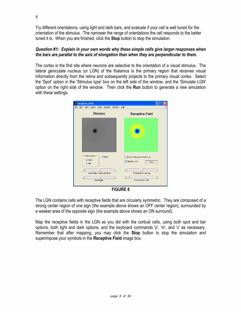
Try different orientations, using light and dark bars, and evaluate if your cell is well tuned for the orientation of the stimulus. The narrower the range of orientations the cell responds to the better tuned it is. When you are finished, click the Stop button to stop the simulation. Question #1: Explain in your own words why these simple cells give larger responses when the bars are parallel to the axis of elongation than when they are perpendicular to them. The cortex is the first site where neurons are selective to the orientation of a visual stimulus. The lateral geniculate nucleus (or LGN) of the thalamus is the primary region that receives visual information directly from the retina and subsequently projects to the primary visual cortex. Select the 'Spot' option in the 'Stimulus type' box on the left side of the window, and the 'Simulate LGN' option on the right side of the window. Then click the Run button to generate a new simulation with these settings.

FIGURE 8

The LGN contains cells with receptive fields that are circularly symmetric. They are composed of a strong center region of one sign (the example above shows an OFF center region), surrounded by a weaker area of the opposite sign (the example above shows an ON surround). Map the receptive fields in the LGN as you did with the cortical cells, using both spot and bar options, both light and dark options, and the keyboard commands 'p', 'm', and 'c' as necessary. Remember that after mapping, you may click the Stop button to stop the simulation and superimpose your symbols in the Receptive Field image box.

9

page 9 of 36

FIGURE 9

Examine how LGN receptive fields respond to light and dark bars of different orientations. Notice that its response does not change with the orientation of the bar. In other words, the response is untuned for orientation. Remember to click the Run/Stop button to start/stop the simulation. Question #2: Explain in your own words why the receptive fields of LGN cells are not selective for the orientation of a stimulus. Question #3: Diagram a possible circuit where inputs from the LGN can be summed together to yield a cortical receptive field with elongated receptive fields. Now it is time to play the Mystery Receptive Fields game! While keeping the 'Simulate LGN' box checked, also check the 'Mystery Receptive Field Test' box. Click the Run button to generate a new simulation where the receptive field is masked (so you can't actually see it).

FIGURE 10

10

page 10 of 36

Map the receptive fields here as you did with the visible cortical and LGN cells, using both spot and bar options, both light and dark options, and the keyboard commands 'p', 'm', and 'c' as necessary. BEFORE you click the Stop button to stop the simulation and reveal the solution with your symbols superimposed in the Receptive Field image box, have an instructor come by to verify that you have correctly mapped them. DO NOT continue until this is complete. AFTER your mapping has been approved, uncheck the ‘Stimulate LGN’ option on the right side of the window. Then click the Run button to generate a new simulation with these settings. Accurately map and have verified TWO mystery cortical receptive fields. Cells in the visual cortex have a spontaneous rate of firing. That is, they will fire at some constant rate even when there is a uniform gray in the Stimulus image box. Uncheck the 'Mystery Receptive Field Test' box on the right side of the window. Then increase the 'Spontaneous rate' slider to the center setting on the right side of the window to allow the cell to fire spontaneously at a baseline rate even in the absence of a visual stimulus. Click the Run button to generate a new simulation with these settings.

FIGURE 11

Now examine how the presence of spontaneous activity influences the resulting mapping of a receptive field. Without a visual stimulus present (here, where no spots or bars are visible within the Stimulus image window), you should hear the cell firing spontaneously at about 4 spikes/sec. Map the receptive fields here as you did with before, using both spot and bar options, both light and dark options, and the keyboard commands 'p', 'm', and 'c' as necessary. Do this a few times with both cortical and LGN cells, and be sure to check your mapping ability by stopping the simulation and observing the superimposed images. Remember to click the Run/Stop button to start/stop each simulation. Now play the Mystery Receptive Fields game again, but at this higher spontaneous rate. Check the ‘Stimulate LGN’ box, and also check the 'Mystery Receptive Field Test' box on the right side of the window. Click the Run button to generate a new simulation where the receptive field is masked (so you can't actually see it).

11

page 11 of 36

Map the receptive fields here as you did before, using both spot and bar options, both light and dark options, and the keyboard commands 'p', 'm', and 'c' as necessary. BEFORE you click the Stop button to stop the simulation and reveal the solution with your symbols superimposed in the Receptive Field image box, have an instructor come by to verify that you have correctly mapped them. DO NOT continue until this is complete. AFTER your mapping has been approved, uncheck the ‘Stimulate LGN’ option on the right side of the window. Then click the Run button to generate a new simulation with these settings. Accurately map and have verified FOUR mystery cortical receptive fields. Question #4: Do you feel it is easier or more difficult to map the receptive field when the cell has a spontaneous rate higher than zero? What did you notice was different? Explain your answer in your own words. Congratulations! You have successfully completed the Part #1 of the lab. In the Part #2, you will begin using more quantitative methods to analyze the tuning properties of these neurons.

12

page 12 of 36

Part #2. To get started, run Matlab by double-clicking the MATLAB R2007b shortcut on the desktop. A MATLAB 7.5.0 (R2007b) window will appear. In the Command Window section, type the following highlighted commands at the prompt (>>), hitting Return on the keyboard after each command. [Note: If you are using a digital copy of this tutorial, you may also copy the highlighted portions and paste them into the Command Window prompt.] cd receptive_field receptive_field_lab(2)

FIGURE 12 A receptive_field window will appear. Click the New receptive field button ONLY ONCE to display a cell’s receptive field.

FIGURE 13

Now click the Run button to initiate the simulation.

13

page 13 of 36

FIGURE 14

The interface is very similar to the one you interacted with in Part #1. The Receptive Field image on the right shows the spatial organization of the receptive field of a simple cortical neuron. Again, areas in red hues indicate ON sub-regions while areas in blue hues indicate OFF sub-regions, and green areas are neutral and thus outside the cell’s receptive field. The Stimulus image on the left once again shows a visual stimulus region on the exact area of the visual field as the receptive field is on the right side of the window. This time, however, you will be implementing well-controlled visual stimuli similar to that used in modern visual experiments, rather than the pattern of flashing lights used by Hubel and Wiesel. Sinusoidal drifting stimuli will be presented which you can control only across three parameters: (1) orientation (or drift direction), (2) spatial frequency, (3) contrast. Sinusoidal drifting stimuli (or sinusoidal grating) are periodic patterns of bright and dark 'bars' of light that are moving (drifting) in a particular direction. The easiest way to grasp this concept is to work with the stimuli by manipulating its parameters. The orientation parameter, which operates as units of degrees, controls the direction of the drift. At 0° the stimuli move from left to right, at 90° the stimuli move from bottom to top, at 180° the stimuli move from right to left, and at 270° the stimuli move from top to bottom. In the 'Orientation' field on the left side of the window type 45, then hit Return on the keyboard. Watch how the directional movement of the stimuli changes.

14

page 14 of 36

FIGURE 15

Now type 270 in the 'Orientation' field, then hit Return on the keyboard. Watch how the directional movement of the stimuli changes again.

FIGURE 16

The spatial frequency parameter controls the number of 'bars' (or cycles) appearing within a given frame (here, the Stimulus image box). In the 'Spatial Frequency' field on the left side of the window type 2.0, then hit Return on the keyboard. Watch how the number of bars (light and dark separately) appearing in the frame decreases from four to two.

15

page 15 of 36

FIGURE 17

In the 'Spatial Frequency' field on the left side of the window type 5.0, then hit Return on the keyboard. Watch how the number of bars (light and dark separately) appearing in the frame increases from two to five.

FIGURE 18

The contrast parameter, which operates as a percent, controls the depth of the luminance (or brightness) modulation in the pattern. One could easily consider it analogous to stimulus 'strength', in that the stronger the contrast is (by using a larger percentage), the bigger the visual contrast between the light and dark bars. At 100% the stimuli display the most contrast, as they are modulated from complete darkness (in the center of the dark bars) to the highest possible luminance achievable by the computer monitor (in the center of the light bars). At 0% the stimuli display the least contrast, and appear as a gray background. In the 'Contrast' field on the left side of the window type 20, then hit Return on the keyboard. Watch how the contrast between light and dark bars decreases.

16

page 16 of 36

FIGURE 19

In the 'Spatial Frequency' field on the left side of the window type 1.5, and in the 'Contrast' field type 100, then hit Return on the keyboard. Stop the simulation by hitting the Stop button once.

FIGURE 20

Notice that this interface provides you with two additional numeric features on the right side of the window. Displayed adjacent to the New receptive field button is the average rate of firing per second that occurred during the last run. In this case, the cell fired an averaged of 4.41 spikes/sec. Displayed adjacent to the Run button is the total run time of the last run. In this case, the cell was actively stimulated for 3735.0 sec. Soon, you will be measuring the mean firing rate of neurons as a function of different stimulus parameters.

17

page 17 of 36

Measuring the orientation tuning curve. Your first goal is to measure the orientation tuning curve of a cell. This is a curve that shows the response of the cell (in spikes/sec) as a function of the stimuli orientation (in degrees). You will be recording the responses for a sequence of angles from 0° to 180°, given in intervals of 20°. A total of ten intervals will be recorded. You will run the simulation for at least 20 sec for these different orientations and record the response rate in each case. Before you begin, click the New receptive field button several times until you have found a receptive field that does NOT look like the one pictured in this tutorial and that does NOT look like your other classmates’ receptive fields, but that DOES have at least one clear ON sub-region and one clear OFF sub-region displaying in the Receptive Field image box. [Note: Since you need to continue working with the same receptive field just generated, it is important that you DO NOT click the New receptive field button again after you’ve found one that is appropriate.] Capture a screen shot of the receptive_field window for your lab report along with an appropriate caption. To do this, press Command-Shift-4 on the keyboard, and use your mouse to select the rectangular area you wish to copy to the computer’s clipboard. A .png file of this image will appear on the Mac Desktop. Rename the file with something descriptive, insert it into a document, and add a caption to label the ON sub-regions and the OFF sub-regions of the receptive field. Go back to the receptive_field window. In the 'Orientation' field on the left side of the window type 0, and in the 'Spatial Frequency' field type 4.0. Click the Run button and allow the simulation to run for at least 20 sec before you hit the Stop button to stop it. Be sure you WRITE DOWN the average rate of firing for your records.

FIGURE 21

In the 'Orientation' field on the left side of the window type 20, then click the Run button and allow the simulation to run for at least 20 sec before you hit the Stop button to stop it. Be sure you WRITE DOWN the average rate of firing for your records.

18

page 18 of 36

Continue to modify the orientation parameter in intervals of 20° (0-done, 20-done, 40, 60, 80, 100, 120, 140, 160, 180), running each for at least 20 sec, until you complete the simulations of all ten orientations (ending at 180°). Make sure you have a written record of all of your values. Once you have compiled a set of orientation-response pairs you can plot them in Matlab. Go to the MATLAB 7.5.0 (R2007b) window. In the Command Window section, input your responses as a list (as shown below) at the prompt (>>). Make sure that your list of ten average firing rates is contained in brackets, in order of orientation from 0° to 180°, each separated by a single space. [Note: The values used in this tutorial are given as example only. Your data should be unique to you. If you are using a digital copy of this tutorial, you may copy and paste the following command into the Command Window prompt, but then you MUST be sure to swap out the sample values for your own.] Hit Return on the keyboard after this command to allow Matlab to input your list. response = [2.16 6.46 11.57 10.15 3.43 0.68 0.20 0.09 0.29 1.48]

FIGURE 22

Next you will need to plot an orientation tuning curve based on your results. In the Command Window section, type the following command at the prompt (>>), then hit Return on the keyboard. figure, plot(0:20:180,response,'b-o'); xlabel('Orientation (degrees)'); ylabel('Response (spikes/sec)')

FIGURE 23

A Figure window will appear, containing the orientation tuning curve of the cell you used. This is a graph of your acquired responses (in spikes/sec) as a function of orientation of the grating (in degrees).

FIGURE 24

19

page 19 of 36

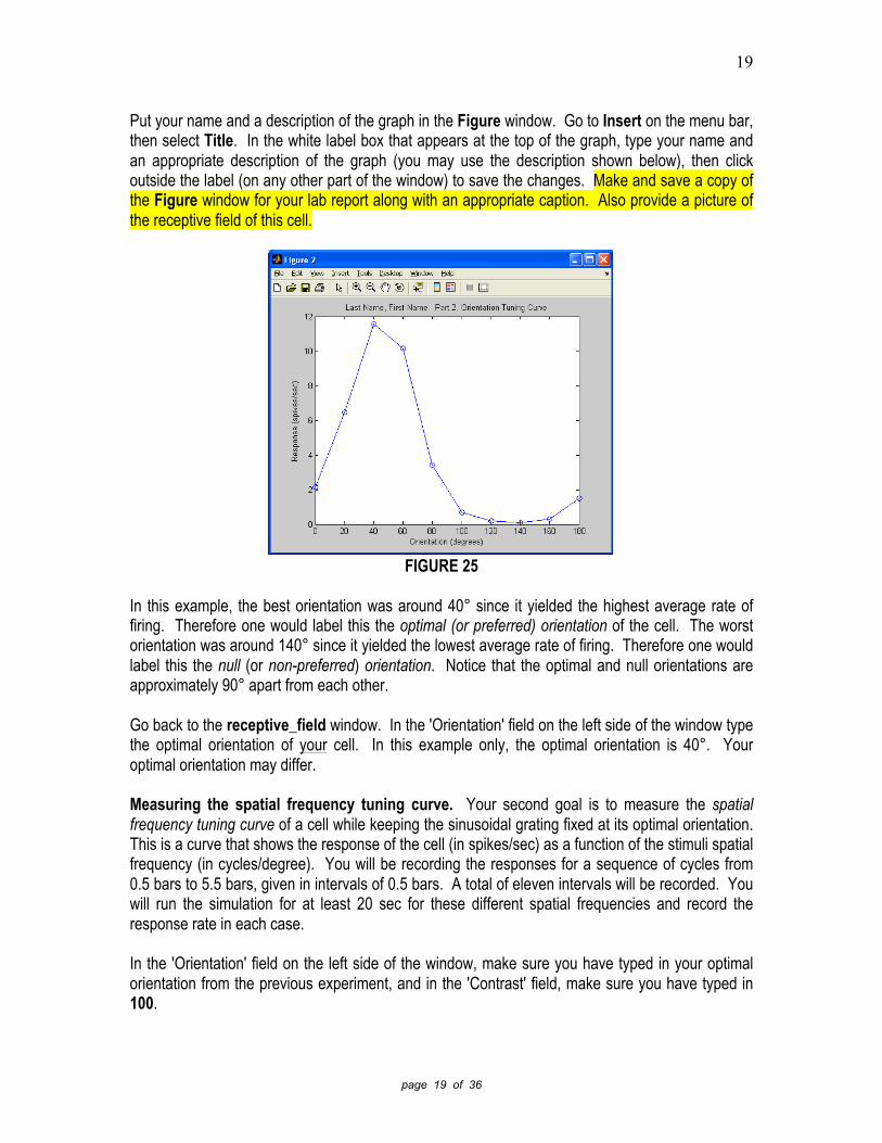
Put your name and a description of the graph in the Figure window. Go to Insert on the menu bar, then select Title. In the white label box that appears at the top of the graph, type your name and an appropriate description of the graph (you may use the description shown below), then click outside the label (on any other part of the window) to save the changes. Make and save a copy of the Figure window for your lab report along with an appropriate caption. Also provide a picture of the receptive field of this cell.

FIGURE 25

In this example, the best orientation was around 40° since it yielded the highest average rate of firing. Therefore one would label this the optimal (or preferred) orientation of the cell. The worst orientation was around 140° since it yielded the lowest average rate of firing. Therefore one would label this the null (or non-preferred) orientation. Notice that the optimal and null orientations are approximately 90° apart from each other. Go back to the receptive_field window. In the 'Orientation' field on the left side of the window type the optimal orientation of your cell. In this example only, the optimal orientation is 40°. Your optimal orientation may differ. Measuring the spatial frequency tuning curve. Your second goal is to measure the spatial frequency tuning curve of a cell while keeping the sinusoidal grating fixed at its optimal orientation. This is a curve that shows the response of the cell (in spikes/sec) as a function of the stimuli spatial frequency (in cycles/degree). You will be recording the responses for a sequence of cycles from 0.5 bars to 5.5 bars, given in intervals of 0.5 bars. A total of eleven intervals will be recorded. You will run the simulation for at least 20 sec for these different spatial frequencies and record the response rate in each case. In the 'Orientation' field on the left side of the window, make sure you have typed in your optimal orientation from the previous experiment, and in the 'Contrast' field, make sure you have typed in 100.

20

page 20 of 36

In the 'Spatial Frequency' field on the left side of the window type 0.5 then click the Run button and allow the simulation to run for at least 20 sec before you hit the Stop button to stop it. Be sure you WRITE DOWN the average rate of firing for your records.

FIGURE 26

Continue to modify the spatial frequency parameter in intervals of 0.5 bars (0.5-done, 1.0, 1.5, 2.0, 2.5, 3.0, 3.5, 4.0, 4.5, 5.0, 5.5), running each for at least 20 sec, until you complete the simulations of all eleven spatial frequencies (ending at 5.5 bars). Make sure you have a written record of all of your values. Once you have compiled a set of spatial frequency-response pairs you can plot them in Matlab. Go to the MATLAB 7.5.0 (R2007b) window. In the Command Window section, input your responses as a list (as shown below) at the prompt (>>). Make sure that your list of eleven average firing rates is contained in brackets, in order of spatial frequency from 0.5 bars to 5.5 bars, each separated by a single space. [Note: The values used in this tutorial are given as example only. Your data should be unique to you. If you are using a digital copy of this tutorial, you may copy and paste the following command into the Command Window prompt, but then you MUST be sure to swap out the sample values for your own.] Hit Return on the keyboard after this command to allow Matlab to input your list. response = [7.49 11.37 17.02 18.74 20.03 19.59 17.01 11.32 6.09 2.76 1.36]

FIGURE 27

Next you will need to plot a spatial frequency tuning curve based on your results. In the Command Window section, type the following command at the prompt (>>), then hit Return on the keyboard. figure, plot(0.5:0.5:5.5,response,'b-o'); xlabel('Spatial Frequency (cycles/degree)'); ylabel('Response spikes/sec)')

FIGURE 28

21

page 21 of 36

A Figure window will appear, containing the spatial frequency tuning curve of the cell you used. This is a graph of your acquired responses (in spikes/sec) as a function of spatial frequency of the grating (in cycles/degree).

FIGURE 29

Put your name and a description of the graph in the Figure window. Go to Insert on the menu bar, then select Title. In the white label box that appears at the top of the graph, type your name and an appropriate description of the graph (you may use the description shown below), then click outside the label (on any other part of the window) to save the changes. Make and save a copy of the Figure window for your lab report along with an appropriate caption.

FIGURE 30

22

page 22 of 36

You can see that, indeed, not all spatial frequencies are equally effective in driving the cell to fire. In this example, the optimal (or preferred) spatial frequency of the cell was around 2.5 cycles/degree. Notice that the response decreases if the spatial frequency is too small or too big. Question #5: Explain in your own words why the spatial frequency tuning curve assumes an inverted 'U' shape. In other words, why is it that the responses are low at both low and high spatial frequencies, and why is there is an intermediate spatial frequency that is optimal? Make and save a copy of your spatial tuning curve with a caption as part of your answer. Go back to the receptive_field window. In the 'Spatial Frequency' field on the left side of the window type the optimal spatial frequency of your cell. In this example only, the optimal spatial frequency is about 2.5. Your optimal spatial frequency may differ. Question #6: Run a simulation with the parameters set at the cell’s optimal orientation and optimal spatial frequency. Listen to the temporal pattern of the spikes. Explain in your own words why the cell fires in little 'bursts' with pauses in between. Measuring the contrast response function (contrast tuning curve). Your third goal is to measure the contrast response function of a cell while keeping the sinusoidal grating fixed at both its optimal orientation and its optimal spatial frequency. This is a curve that shows the response of the cell (in spikes/sec) as a function of the stimuli contrast (in percent). You will be recording the responses for a sequence of percentages from 0% to 100%, given in intervals of 10%. A total of eleven intervals will be recorded. You will run the simulation for at least 20 sec for these different contrasts and record the response in each case. In the 'Orientation' field on the left side of the window, make sure you have typed in your optimal orientation from the previous experiment, and in the 'Spatial Frequency' field, make sure you have typed in you optimal spatial frequency from the previous experiment. In the 'Contrast' field on the left side of the window type 0 then click the Run button and allow the simulation to run for at least 20 sec before you hit the Stop button to stop it. Be sure you WRITE DOWN the average rate of firing for your records.

23

page 23 of 36

FIGURE 31

Continue to modify the contrast parameter in intervals of 10% (0-done, 10, 20, 30, 40, 50, 60, 70, 80, 90, 100), running each for at least 20 sec, until you complete the simulations of all eleven contrasts (ending at 100%). Make sure you have a written record of all of your values. Once you have compiled a set of contrast-response pairs you can plot them in Matlab. Go to the MATLAB 7.5.0 (R2007b) window. In the Command Window section, input your responses as a list (as shown below) at the prompt (>>). Make sure that your list of eleven average firing rates is contained in brackets, in order of contrast from 0% to 100%, each separated by a single space. [Note: The values used in this tutorial are given as example only. Your data should be unique to you. If you are using a digital copy of this tutorial, you may copy and paste the following command into the Command Window prompt, but then you MUST be sure to swap out the sample values for your own.] Hit Return on the keyboard after this command to allow Matlab to input your list. response = [0.00 2.02 5.04 8.01 10.82 13.20 15.59 17.34 18.43 18.75 20.36]

FIGURE 32

Next you will need to plot a contrast tuning curve based on your results. In the Command Window section, type the following command at the prompt (>>), then hit Return on the keyboard. figure, plot(0:10:100,response,'b-o'); xlabel('Contrast (percent)'); ylabel('Response (spikes/sec)')

FIGURE 33

A Figure window will appear, containing the contrast response function of the cell you used, a graph of your acquired responses (in spikes/sec) as a function of contrast of the grating (in percents).

24

page 24 of 36

FIGURE 34

Put your name and a description of the graph in the Figure window. Go to Insert on the menu bar, then select Title. In the white label box that appears at the top of the graph, type your name and an appropriate description of the graph (you may use the description shown below), then click outside the label (on any other part of the window) to save the changes. Make and save a copy of the Figure window for your lab report along with an appropriate caption.

FIGURE 35

In this example, the optimal (or preferred) contrast of the cell was at 100%. Notice that the responses increase linearly as the contrasts (stimuli strengths) increase.

25

page 25 of 36

The effect of spike threshold on orientation tuning curves: Your fourth goal is to study how orientation tuning depends on the threshold of the cell. Loosely speaking, the threshold represents the level of activity inside the cell (termed the generator potential) that is necessary to fire a spike. If the threshold is too high the cell may only fire sporadically and, of course, you will not see much in the spike train that reflects the underlying tuning properties of the generator potential. The smaller the threshold is, the more the spike rate will follow the tuning of the underlying generator potential. In the 'Spatial Frequency' field on the left side of the window, make sure you have typed in your optimal spatial frequency from the previous experiment, and in the 'Contrast' field, make sure you have typed in you optimal contrast from the previous experiment. Go back to the receptive_field window. The threshold (in percent) can be increased/decreased using the slider labeled 'Threshold for spiking' on the right side of the window. Leaving the 'Threshold for spiking' slider in the center setting (just above the letter ‘d’ in the word ‘Threshold’; around 50%), measure the orientation tuning curve of the cell as you did earlier (running at least 20 sec for every 20° orientation from 0° to 180°). Make sure you record the responses for all ten intervals and label them 'low_threshold'.

FIGURE 36

Now move the 'Threshold for spiking' slider so that it sits 75% to the right (just above the letter ‘k’ in the word ‘spiking’), thereby increasing the threshold. Again, measure the orientation tuning curve of the cell as you did earlier (running at least 20 sec for every 20° orientation from 0° to 180°). Make sure you record all the responses for all ten intervals and label them 'high_threshold'.

26

page 26 of 36

FIGURE 37

Go back to the MATLAB 7.5.0 (R2007b) window. In the Command Window section, input your responses as a list (as shown below) at the prompt (>>). Notice that you will be importing two separate lists (one for 'response_low' and one for 'response_high'), hitting Return on the keyboard after each command. [Note: The values used in this tutorial are given as example only. Your data should be unique to you. If you are using a digital copy of this tutorial, you may copy and paste the following commands into the Command Window prompt, but then you MUST be sure to swap out the sample values for your own.] low_threshold = [7.94 17.86 20.28 19.61 13.82 5.72 1.86 0.34 3.34 8.99]

high_threshold = [0.00 11.35 16.27 15.69 4.69 0.00 0.00 0.00 0.00 0.00]

FIGURE 38 Next plot the corresponding orientation tuning curves based on your results. In the Command Window section, type the following command at the prompt (>>), then hit Return on the keyboard. figure, plot(0:20:180,low_threshold,'b-o'); xlabel('Orientation (degrees)'); ylabel('Response (spikes/sec)')

hold on

plot(0:20:180,high_threshold,'r--*'); xlabel('Orientation (degrees)'); ylabel('Response (spikes/sec)')

FIGURE 39

A Figure window will appear, containing the orientation tuning curves of the cell you used. These are graphs of your acquired responses (in spikes/sec) as a function of orientation of the grating (in degrees).

27

page 27 of 36

FIGURE 40

Put your name and a description of the graph in the Figure window. Go to Insert on the menu bar, then select Title. In the white label box that appears at the top of the graph, type your name and an appropriate description of the graph (you may use the description shown below), then click outside the label (on any other part of the window) to save the changes. Include a legend for the graph as well. Go to Insert on the menu bar, then select Legend. Replace the existing legend labels with something more descriptive. Make and save a copy of the Figure window for your lab report along with an appropriate caption.

FIGURE 41

In this example, the orientation tuning curve with higher response values corresponds to the measurements you made at a lower threshold, and the orientation tuning curve with lower response values corresponds to the measurements you made at a higher threshold.

28

page 28 of 36

Question #7: Which curve is better tuned, the curve measured at a lower threshold or the curve measured at a higher threshold? That is, which curve shows a response for a smaller range of orientations? How can the different thresholds have such an effect on the orientation tuning curve? Explain your answers in your own words. Good job! You are now ready for Part #3 of the lab!

29

page 29 of 36

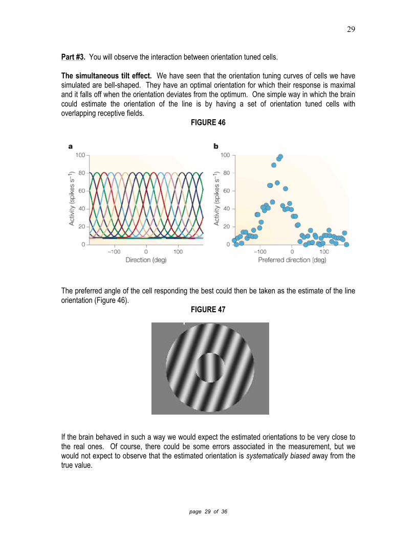
Part #3. You will observe the interaction between orientation tuned cells. The simultaneous tilt effect. We have seen that the orientation tuning curves of cells we have simulated are bell-shaped. They have an optimal orientation for which their response is maximal and it falls off when the orientation deviates from the optimum. One simple way in which the brain could estimate the orientation of the line is by having a set of orientation tuned cells with overlapping receptive fields.

FIGURE 46

The preferred angle of the cell responding the best could then be taken as the estimate of the line orientation (Figure 46).

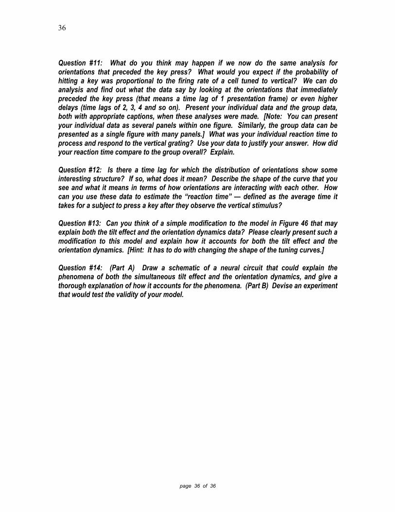
FIGURE 47

If the brain behaved in such a way we would expect the estimated orientations to be very close to the real ones. Of course, there could be some errors associated in the measurement, but we would not expect to observe that the estimated orientation is systematically biased away from the true value.

30

page 30 of 36

It turns out, however, that systematic biases are indeed observed in many situations. Such phenomena are usually called “visual illusions.” One classic example is the simultaneous tilt effect, where the orientation of a central patch is influenced by that of the surround (Figure 47). In this case, the perceived orientation of a central patch containing a vertical grating is biased away from vertical depending on the orientation of the surround. It is as if the two orientations are “repelling” each other away. The actual (vertical) orientation of the central patch is different from the perceived (illusory) orientation. As we noted above, this is not what would one expect by a simple decoding mechanisms the one shown in Figure 46. The finding suggests that orientation tuned detectors may be interacting in some interesting ways. For our first experiment we are going to measure how the perceived orientation of a central patch is influenced by one simultaneously presented in the surround. We will use the program “orientation_tilt” to do this. During the entire experiment you will keep a viewing distance to the screen that is about 50-60 cm. Start the program now. Once you start the program a uniform grating will first appear. You will adjust the orientation of the central patch so that it looks as close to vertical as possible by rotating it clockwise (‘w’ - coarse, ’s’ - fine) or counter-clockwise (‘q’ coarse, ‘a’ - fine). Try to do these adjustments by first using the coarse controls (w & q) and then making fine adjustment near the vertical using the fine controls (a & s). Once you are satisfied with the orientation of the central patch hit the ’n’ key to get a new trial with a different orientation of the surround. The adjustment period should not last more than 15-20s. Each of you will run a session for 20 min. The data you just collected was saved in a file named ‘data.txt’. Change its name to be your full name while keeping the file extension ‘txt’. You will be instructed on how to send this file to the instructors. Then the data from the group will be pooled together and distributed back to you for analysis. Each row in the data file contains two numbers. The first is the orientation of the surround. The second is the orientation of the central patch that is perceived as being vertical. To process the data we will use the Matlab function “orientation_tilt”. Start up Matlab and, when you get the command prompt ‘>>’ call the function with the name of the datafile: >> orientation_tilt(‘pooled_data.txt’)

FIGURE 48 The x-axis represents the orientation of the surround, while the y-axis represents the corresponding orientation of the center that yields a percept of a vertical orientation.

31

page 31 of 36

Now answer the following questions. Question #8: If the null hypothesis is that the surround has no influence on the perception of the central patch, what would be the expected shape of the graph? Question #9: Does the data conform to the null hypothesis? If not, how does it depart from the expected result of the null hypothesis? What does the departure mean in terms of how the orientations interact? Present your individual data and the group data, both with appropriate captions, as part of your answer. In the simultaneous tilt effect we are observing how two orientations, in different parts of the image, interact with each other. What about orientations presented sequentially on the same location? Do they interact? That is the question we will answer in the next experiment. Orientation dynamics. In this experiment you will be presented by a rapid sequence of oriented gratings. The task is very simple. Every time you see a grating that is vertical you have to press a key to indicate that you saw it. That’s all! It sounds easy, right? Well, it turns out that when the images are presented at a high rate (in this case about 10 per second) you must really pay attention and the task becomes rather demanding. While performing this task you do not have to worry about detecting every single vertical grating, but just make sure that your respond only if you see one. In other words, missing a few gratings is Ok but we do not want to see many mistakes. Start the program “randori.” This immediately will start running the orientation sequence. Whenever you see a vertical grating hit the spacebar. Each of you will run the sequence for 10 min. We know this may be tiring, so please relax, sit back, and do the best you can. At the end of the run there will be a file named “data.txt”. Each row in this file contains the orientation presented and a zero or a one depending on whether the space bar was pressed during its presentation. Change the name to your name and keep the extension “data.txt”. You will be instructed as to how to share this file with the instructors. When you are all done, a merged file containing the pooled data of all the students will be sent back to you. Of course, it takes some time between the time you see a visual target and the time you press the key.

32

page 32 of 36

Question #10: Given that there is this known sensorimotor delay, if we now pull all the orientations from the data file that have a ‘1’ next to them (the orientations present when a key press occurs), what would be their expected distribution and why? Verify your answer by executing in Matlab: >> orientation_dynamics(‘pooled_data.txt’,0)

FIGURE 49 The result is a plot showing the number of times each orientation was presented at the same time of a key press (a distribution of orientations). Question #11: What do you think may happen if we now do the same analysis for orientations that preceded the key press? What would you expect if the probability of hitting a key was proportional to the firing rate of a cell tuned to vertical? We can do analysis and find out what the data say by looking at the orientations that immediately preceded the key press (that means a time lag of 1 presentation frame) or even higher delays (time lags of 2, 3, 4 and so on). Present your individual data and the group data, both with appropriate captions, when these analyses were made. [Note: You can present your individual data as several panels within one figure. Similarly, the group data can be presented as a single figure with many panels.] What was your individual reaction time to process and respond to the vertical grating? Use your data to justify your answer. How did your reaction time compare to the group overall? Explain. To find out what the data show, call the Matlab function: >> orientation_dynamics(‘pooled_data.txt’,1) >> orientation_dynamics(‘pooled_data.txt’,2) >> orientation_dynamics(‘pooled_data.txt’,3)

FIGURE 50 And so on. Question #12: Is there a time lag for which the distribution of orientations show some interesting structure? If so, what does it mean? Describe the shape of the curve that you see and what it means in terms of how orientations are interacting with each other. How can you use these data to estimate the “reaction time” — defined as the average time it takes for a subject to press a key after they observe the vertical stimulus? Question #13: Can you think of a simple modification to the model in Figure 46 that may explain both the tilt effect and the orientation dynamics data? Please clearly present such a modification to this model and explain how it accounts for both the tilt effect and the orientation dynamics. [Hint: It has to do with changing the shape of the tuning curves.]

33

page 33 of 36

34

page 34 of 36

Question #14: (Part A) Draw a schematic of a neural circuit that could explain the phenomena of both the simultaneous tilt effect and the orientation dynamics, and give a thorough explanation of how it accounts for the phenomena. (Part B) Devise an experiment that would test the validity of your model. Hooray! You are now finished with the tutorial! That's all folks! The goal of the lab was to give you an idea of how neuroscientists are investigating how is that the brain processes sensory information. This not only will allow you to understand normal brain processing but also what goes wrong during central diseases of vision. The basic information scientists have gathered about the early stages of visual processing is now being used to developed visual prostheses to restore sight in blind patients (and Geordi La Forge will no longer be a science fiction character). To read more see: http://www.usc.edu/uscnews/stories/14864.html

35

page 35 of 36

Lab Report Questions. Please provide a clear but concise response to the following questions. Be sure to included supporting figures with proper labels and descriptions. Question #1: Explain in your own words why these simple cells give larger responses when the bars are parallel to the axis of elongation than when they are perpendicular to them. Question #2: Explain in your own words why the receptive fields of LGN cells are not selective for the orientation of a stimulus. Question #3: Diagram a possible circuit where inputs from the LGN can be summed together to yield a cortical receptive field with elongated receptive fields. Question #4: Do you feel it is easier or more difficult to map the receptive field when the cell has a spontaneous rate higher than zero? What did you notice was different? Explain your answer in your own words. Question #5: Explain in your own words why the spatial frequency tuning curve assumes an inverted 'U' shape. In other words, why is it that the responses are low at both low and high spatial frequencies, and why is there is an intermediate spatial frequency that is optimal? Make and save a copy of your spatial tuning curve with a caption as part of your answer. Question #6: Run a simulation with the parameters set at the cell’s optimal orientation and optimal spatial frequency. Listen to the temporal pattern of the spikes. Explain in your own words why the cell fires in little 'bursts' with pauses in between. Question #7: Which curve is better tuned, the curve measured at a lower threshold or the curve measured at a higher threshold? That is, which curve shows a response for a smaller range of orientations? How can the different thresholds have such an effect on the orientation tuning curve? Explain your answers in your own words. Question #8: If the null hypothesis is that the surround has no influence on the perception of the central patch, what would be the expected shape of the graph? Question #9: Does the data conform to the null hypothesis? If not, how does it depart from the expected result of the null hypothesis? What does the departure mean in terms of how the orientations interact? Present your individual data and the group data, both with appropriate captions, as part of your answer. Question #10: Given that there is this known sensorimotor delay, if we now pull all the orientations from the data file that have a ‘1’ next to them (the orientations present when a key press occurs), what would be their expected distribution and why?

36

page 36 of 36

Question #11: What do you think may happen if we now do the same analysis for orientations that preceded the key press? What would you expect if the probability of hitting a key was proportional to the firing rate of a cell tuned to vertical? We can do analysis and find out what the data say by looking at the orientations that immediately preceded the key press (that means a time lag of 1 presentation frame) or even higher delays (time lags of 2, 3, 4 and so on). Present your individual data and the group data, both with appropriate captions, when these analyses were made. [Note: You can present your individual data as several panels within one figure. Similarly, the group data can be presented as a single figure with many panels.] What was your individual reaction time to process and respond to the vertical grating? Use your data to justify your answer. How did your reaction time compare to the group overall? Explain. Question #12: Is there a time lag for which the distribution of orientations show some interesting structure? If so, what does it mean? Describe the shape of the curve that you see and what it means in terms of how orientations are interacting with each other. How can you use these data to estimate the “reaction time” — defined as the average time it takes for a subject to press a key after they observe the vertical stimulus? Question #13: Can you think of a simple modification to the model in Figure 46 that may explain both the tilt effect and the orientation dynamics data? Please clearly present such a modification to this model and explain how it accounts for both the tilt effect and the orientation dynamics. [Hint: It has to do with changing the shape of the tuning curves.] Question #14: (Part A) Draw a schematic of a neural circuit that could explain the phenomena of both the simultaneous tilt effect and the orientation dynamics, and give a thorough explanation of how it accounts for the phenomena. (Part B) Devise an experiment that would test the validity of your model.