visual tthymo - visualotthymo.comvisualotthymo.com/downloads/reference manual - vo5.pdf · 1.3 time...
TRANSCRIPT

VISUAL OTTHYMO
REFERENCE MANUAL
VERSION 5.0
Civica Infrastructure Inc. March 2017

iii
CONTENTS
1 Tips for Modelling Ungauged Rural Catchments 1
1.1 Initial Abstraction Parameter, IA 1
1.1.1 Modified Curve Number Method (CN*) 1
1.1.2 SCS Method (CN) 1
1.2 Modified Curve Number, CN* 1
1.3 Time to Peak Parameter, TP 2
1.3.1 Upland’s Method 3
1.3.2 Bransby - William’s Formula 3
1.3.3 Airport Method 3
1.3.4 William’s Equation (1977) 4
2 Tips for Modelling Ungauged Urban Catchments 5
2.1 Imperviousness 5
2.2 Loss Routine 6
2.3 Parameters for the Pervious Component 6
2.4 Parameters for the Impervious Component 7
3 SWM Pond Modelling 8
3.1 How to Build a Rating Curve Using ROUTE RESERVOIR 8
4 Computation of Rainfall Losses 10
4.1 Critical Review of SCS Curve Number Procedure 10
4.1.1 Critical Review of SCS Curve Number Procedure 10
4.2 Calibration of the Modified SCS CN Procedure 14
4.3 Infiltration Procedures in STANDHYD 19
4.3.1 Horton's Equation 19
4.3.2 Modified CN Procedure 20
4.4 Considerations in Using the Rainfall Losses 20

iv
5 Unit Hydrograph Options In Visual OTTHYMO 24
5.1 IUH Relations 25
5.2 The STANDARD IUH 26
5.3 The NASH IUH (NASHYD) 28
5.4 The SCS IUH (SCSHYD) 28
5.5 The WILLIAMS IUH 29
5.6 Use of IUH’s For I/I Simulation and Baseflow (DWF) 30
5.7 Unit Hydrograph Options for Rural Areas 30
5.7.1 Instantaneous Unit Hydrograph 30
5.7.2 Estimation of Time to Peak (𝒕𝒑) in NASHYD 32
5.7.3 William’s Unit Hydrograph 32
6 Routing Options In Visual OTTHYMO 35
6.1 Simulation Time Steps 35
6.2 Time Shift Routing 36
6.3 Variable Storage Coefficient Routing in Visual OTTHYMO 36
6.4 Muskingum-Cunge Channel Routing 36
6.4.1 Basic Flow Equations 37
6.4.2 Solution of Flow Equations 38
6.4.3 Data Requirements 39
6.4.4 Simulation Results 39
7 Design Storms For Stormwater Management Studies 41
7.1 Methodology Of Design Storms 44
7.1.1 Results for the Chicago Design Storm 44
7.2 Methodology for Comparing Design Storms and a Historical Storm Series 46
7.2.1 Rainfall Input 46
7.2.2 Watersheds Studied 48
7.2.3 Simulation Models and their Calibration 49
7.3 Results Of Peak Flows From Design Storms And Historic Storm Events 50
7.3.1 Rural Watersheds 50
7.3.2 Urban Watersheds 53
v
7.3.3 Mixed Land Use Watershed 56
7.4 Conclusions 57
8 A Review Of Design Storm Profiles 59
8.1 Intensity Duration Frequency Curves 59
8.2 Frequency Of Real Storms And Synthetic Storms 60
8.3 Uniform Design Storm 61
8.4 Composite Design Storm 62
8.5 Chicago Design Storm 62
8.5.1 Derivation of the Chicago Design Storm 62
8.5.2 Parameter Estimation 64
8.5.3 Determination of the Chicago Design Storm Hyetograph 65
8.6 SCS 24-Hour Design Storm 65
8.7 SCS 6 Hour Design Storm 66
8.8 Illinois State Water Survey Design Storm 67
8.9 Atmospheric Environment Service Design Storm 70
8.10 Flood Studies Report Design Storm 72
8.11 Pilgrim and Cordery Design Storm 73
8.12 Yen and Chow Design Storm 74
9 Water Balance Processes in Continuous Simulation 76
9.1 Climate Data 76
9.1.1 Precipitation Data 76
9.1.2 Temperature Data 76
9.1.3 Evaporation Data 77
9.2 Snow Pack Water Balance 80
9.2.1 Initial Condition 80
9.2.2 New Snow Additions 80
9.2.3 Snowmelt 81
9.2.4 Rainfall 82
9.2.5 Refreeze of snowpack liquid water 83
9.2.6 Snowpack Compaction 83

vi
9.2.7 Release of Liquid Water 84
9.3 Depression Storage Water Balance 84
9.4 Active Soil Zone Water Balance 85
9.4.1 Water Contributed from Indirectly Connected Impervious Area 85
9.4.2 Runoff 85
9.4.3 Evapotranspiration 86
9.4.4 Groundwater Infiltration 87
Reference 89

Civica Infrastructure Inc.
Visual OTTHYMO Reference Manual | Page 1
1 TIPS FOR MODELLING UNGAUGED RURAL CATCHMENTS
This section outlines different methodologies for modelling ungauged rural catchments. While it
is preferable to use a calibrated hydrologic model for water resources studies, especially for rural
catchments, this is not always possible. Satisfactory results may still be obtained for macro level
studies provided that the modeller chooses the appropriate parameters for each catchment.
The focus of this section is on the Initial Abstraction parameter, IA, and the Time to Peak param-
eter, TP, parameter. While the CN parameter plays a large role in determining the runoff charac-
teristics of a particular catchment, this parameter can be readily determined and is rarely in dis-
pute by watershed regulating authorities. Guidance is provided in this section on determining the
Modified CN parameters, called CN*.
1.1 INITIAL ABSTRACTION PARAMETER, IA
1.1.1 MODIFIED CURVE NUMBER METHOD (CN*)
When using the Modified Curve Number Method the IA parameter should be set to a value in the
range of 1.0 mm and 5.0 mm, depending on the circumstances. The IA value must then be used
to calculate CN* (see below).
1.1.2 SCS METHOD (CN)
When using the SCS Curve Number Method, IA should be set to 0.2S where S is the soil storage
(a function of CN). Bear in mind that this method may underestimate the peak flow for small
storms because the initial abstraction is higher than the total rainfall, which is not accurate. A
literature review of this method has found that for lower CN values, a lower IA should be used.
Suggests guidelines are as follows:
CN ≤ 70 IA = 0.075S
CN > 70 ≤ 80 IA = 0.10S
CN > 80 ≤ 90 IA = 0.15S
CN > 90 IA = 0.2S
Please note that the above guidelines are for the SCS Method only, where the SCS Curve Num-
ber is used to define the soil type.
1.2 MODIFIED CURVE NUMBER, CN*
The Modified Curve Number method was first proposed by Paul Wisner & Associates in 1982,
and was based on their research and monitoring of rural and urban catchments in Canada. This
method has been used successfully in Canada for the past 35 years and has correlated well with
measured flows.

Civica Infrastructure Inc.
Visual OTTHYMO Reference Manual | Page 2
Rather than having a varying IA parameter, as in the SCS method, the IA is fixed, as described
above, and the CN is altered. The modified CN, called CN* is a function of the IA, and total rainfall.
CN* is calculated as follows:
1. Select an appropriate IA (see above) for catchments being modelled.
2. Determine the SCS CN value from soils maps and/or calculations. Convert the CN (AMC
II conditions) to a CN (AMC III conditions).
3. Determine the largest precipitation volume, P, for a rainfall event that would just represent
AMC III soil moisture conditions. In most cases this is the 100 year storm event. For ex-
ample, in Markham Ontario the 100 year storm volume for the 3 hour storm is 80 mm.
4. Calculate the soil storage S, based on the SCS Method using CN (AMC III conditions).
The metric equation is S = (25400 / CN) –254 and the imperial equation is S = (1000 / CN)
– 10. This will give you the soil storage during your large storm event.
5. Calculate the IA based on the SCS Method, where IA = 0.2S. Note that this relationship
is also valid for the Modified CN Method because it is assumed that the runoff volume, Q,
for large events is the same using both methods.
6. Determine the runoff volume, Q, based on the familiar:
Q = (P – IA)2 / (P - IA + S)
7. Next calculate S* using the above equation again but this time setting IA to the value
calculated for the Modified CN method (i.e. 1.0mm to 5.0mm). This IA will be the value
used in the model simulations.
8. Once you have calculated S*, calculate CN* from the equation:
S* = (25400 / CN*) –254 metric
S* = (1000 / CN*) – 10 imperial
9. The above calculation will give you the CN* for AMC III soil conditions. You now finally
determine the CN* for AMC II soil conditions by using published tables relating CN for
AMC II and AMC III conditions.
The above method is easily adaptable to a spreadsheet so that for future uses, you can easily
and quickly calculate the CN* once you know the IA, P, and CN.
This process has been incorporated in the Convert to CN* tool in Visual OTTHYMO. For more
information, see Appendix A.1 in the User’s Manual.
1.3 TIME TO PEAK PARAMETER, TP
Unlike the urban catchments hydrographs, rural catchment unit hydrographs do not calculate the
time to peak TP as a function of the other variables. The TP parameter must therefore be deter-
mined by the modeller. It should be noted that most methods of estimate TP, start by calculating
the time of concentration, tc. Time of concentration is the time at which the centroid of the flow
reaches the bottom of a catchment. TP is usually a fixed ratio of tc, depending on the unit hydro-
graph chosen.
Over the past 40 years there have been numerous studies in both the United States and Canada
in which empirical, semi-empirical, and mathematical relationships for tc have been derived. Most
of the relationships state that tc is a function of catchment slope, catchment area, and ground

Civica Infrastructure Inc.
Visual OTTHYMO Reference Manual | Page 3
cover. While no single method can be used for every situation we have included the most common
methods in this manual so that the modeller can choose what is appropriate for their situation.
Listed below are five methods for calculating TP. We have included both the source of the method
as well as the context in which it was derived. This way the modeller should be able to choose a
method that was derived for a similar situation as their own.
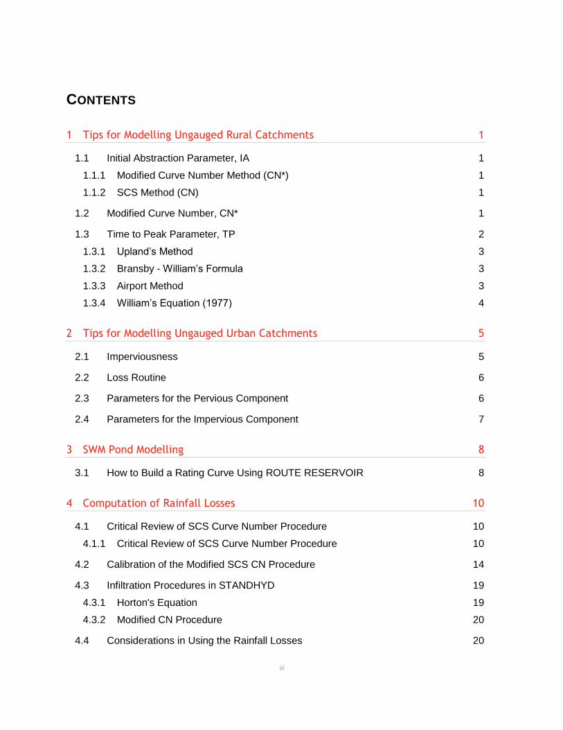
1.3.1 UPLAND’S METHOD
With Upland’s Method the average overland flow velocity is determined for a catchment based on
the catchment slope and ground type, as shown in Figure 1. Once the velocity has been deter-
mined then the time of concentration is determined by dividing the catchment length by the over-
land flow velocity.
1.3.2 BRANSBY - WILLIAM’S FORMULA
In catchments where the runoff coefficient, C, is greater than 0.40, the Bransby Williams formula
is a popular choice. The method calculates time of concentration as a function of catchment area,
length, and slope as follows:
𝑡𝑐 =0.057 ∗ 𝐿
𝑆𝑤0.2 ∗ 𝐴0.1
(1)
where:
𝑡𝑐 = time of concentration (min)
𝐿 = catchment length, (m)
𝑆𝑤 = catchment slope (%)
𝐴 = catchment area (ha)
1.3.3 AIRPORT METHOD
For catchments where the runoff coefficient, C, is less than 0.40, the Airport formula may provide
a better estimate of the time of concentration. This method was developed for airfields and calcu-
lates time of concentration as a function of runoff coefficient, length, and slope as follows:
𝑡𝑐 =3.26 ∗ (1.1 − 𝐶) ∗ 𝐿0.5
𝑆𝑤0.33 (2)
where:
𝑡𝑐 = time of concentration (min)
𝐶= runoff coefficient
𝐿 = catchment length, (m)
𝑆𝑤 = catchment slope (%)
Civica Infrastructure Inc.
Visual OTTHYMO Reference Manual | Page 4
FIGURE 1 UPLANDS METHOD OF ESTIMATING TIME OF CONCENTRATION (SCS NATIONAL EN-
GINEERING HANDBOOK, 1971)
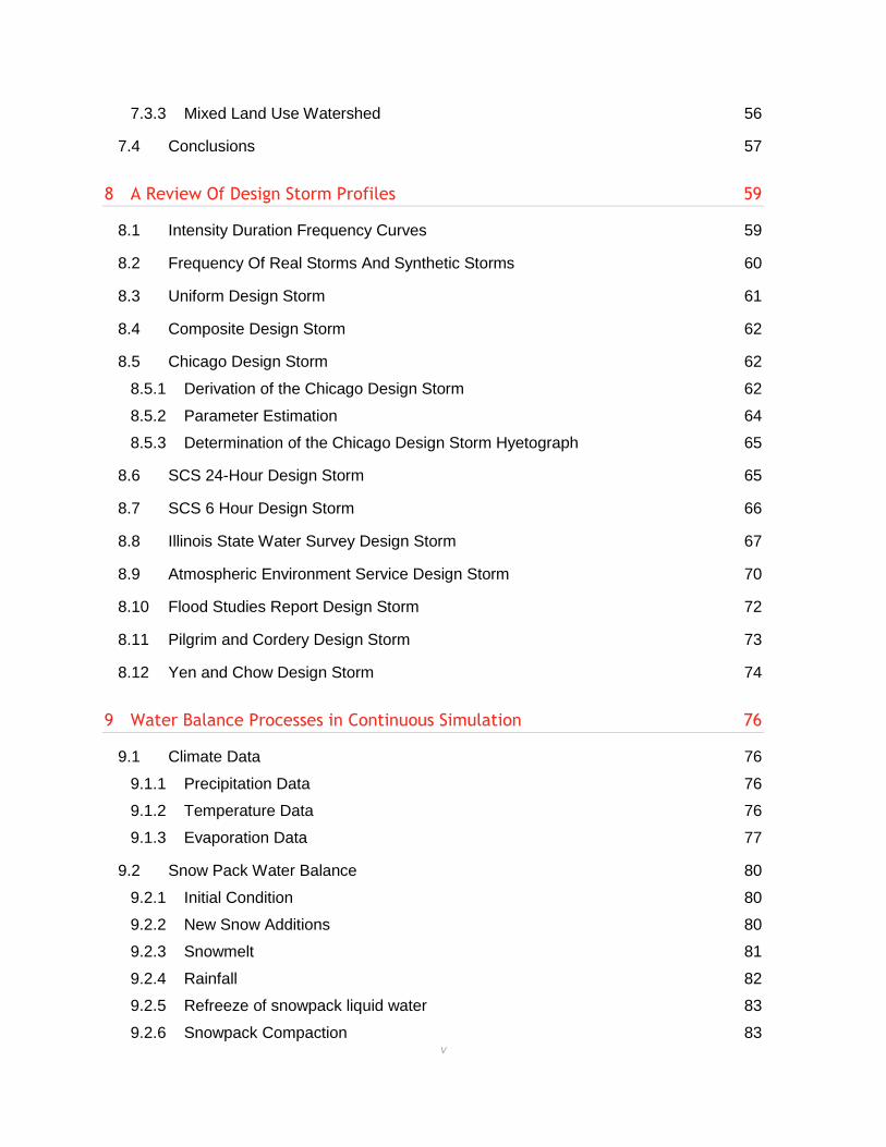
1.3.4 WILLIAM’S EQUATION (1977)
Williams, who co-developed the William’s Unit Hydrograph (WILHYD in Visual OTTHYMO) with
Hann in 1973 later derived empirical relationships for both the K and TP variables in WILHYD.
These relationships are:
𝐾 = 16.14𝐴0.24𝑆−0.84 (3)
𝑡𝑝 = 6.54𝐴0.39𝑆−0.50 (4)
The above relationships were derived for watersheds in the southern United States. Refer to the
Theory Reference section of this manual for more information on the derivation of the WILHYD
unit hydrograph.
Civica Infrastructure Inc.
Visual OTTHYMO Reference Manual | Page 5
2 TIPS FOR MODELLING UNGAUGED URBAN CATCHMENTS
This section provides direction for modellers who are modelling ungauged urban catchments. In
most cases, urban catchments are not gauged since the response to rainfall can be accurately
simulated. However, like any model the user should be aware that the inappropriate selection of
parameters can lead to erroneous output. This section will guide the modeller in selecting param-
eters that have been successfully used in the water resources industry.
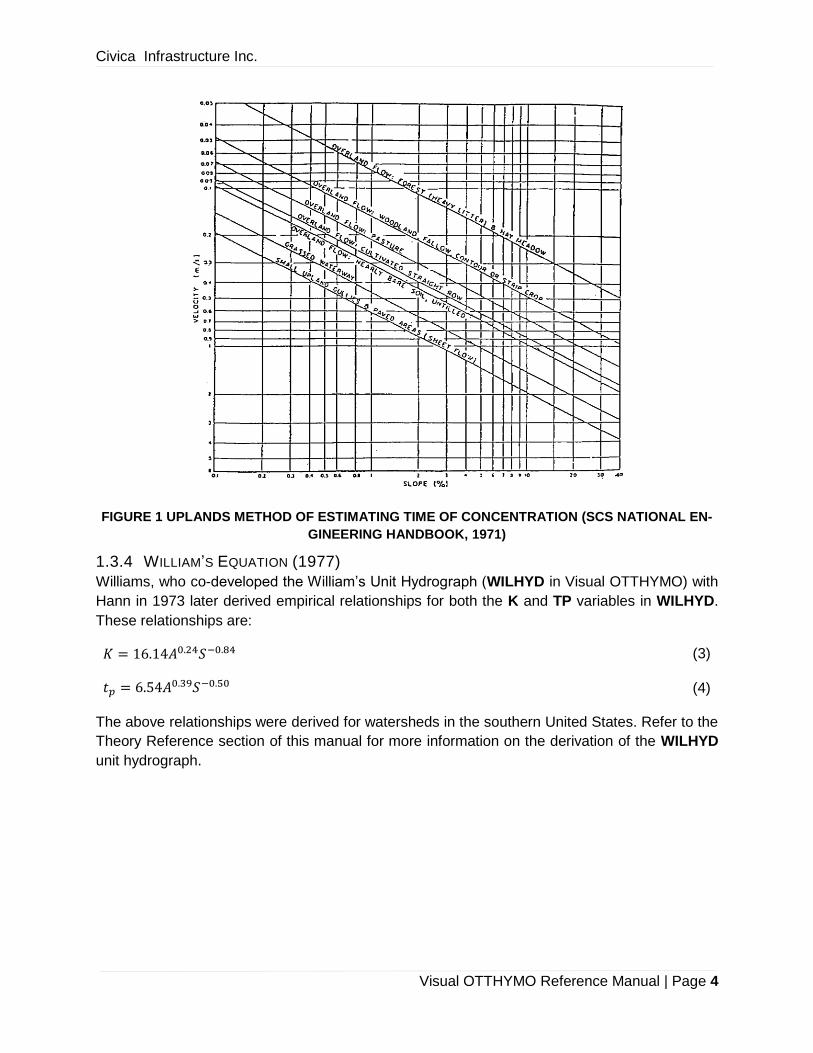
2.1 IMPERVIOUSNESS
There are two impervious ratios required, the amount of directly connected imperviousness,
XIMP, and the total imperviousness, TIMP. XIMP must be less than or equal to TIMP.
TIMP is a function of the land use of the catchment. Land use is a planning term that describes
the approved, or proposed, use for the catchment (e.g. residential, commercial, industrial). Water
resources studies are generally tied to planning applications and depending on the level of plan-
ning application, (i.e. Secondary Plan, Official Plan Amendment, Draft Plan), the modeller will
have a little or a lot of information about the land use. Therefore it is important to select a con-
servative value for the imperviousness when performing more macro level studies so that when
the subsequent more detailed studies are completed, the more refined land use calculations will
still be valid in the overall model.
The following table gives examples of suggested TIMP and XIMP values, based on land use, for
the macro-level studies. These values can be used with the information supplied by the planner
to determine area weighted values for the catchment of interest.
Land Use XIMP TIMP
Estate Residential 20 40
Low Density Residential (e.g. Single Units) 25 50
Medium Density Residential (e.g. Semi-detached Units) 35 55
High Density Residential (e.g. Townhouse Units) 50 60
School 55 55
Commercial 85 85
Park 0 0
For more detailed level studies (i.e. Site Plan), there should be more information available so that
the XIMP and TIMP can be calculated.

Civica Infrastructure Inc.
Visual OTTHYMO Reference Manual | Page 6
2.2 LOSS ROUTINE
In both the United States and Canada, either the Horton’s Method (LOSS = 1) or the CN Method
(LOSS = 2) are commonly used for urban catchments. The Proportional Loss Method (LOSS =
3) has been successfully used in France for urban catchments. While the selection of Loss Rou-
tine can be somewhat arbitrary and at the discretion of the user, there are a few things to keep in
mind when choosing a loss routine.
Horton’s Method is what is used in the SWMM model, therefore if the user is comparing results
with a SWMM based model, or working in a watershed where the overall model used was SWMM,
then this method may be the most appropriate. However, the user should bear in mind that for
longer duration storms (greater than or equal to 12 hours) the Horton’s Method may not accurately
predict the runoff from pervious areas. We have seen cases where the model simulates no runoff
from a pervious area during a 12 hour 100 year storm. This is clearly erroneous. The CN Method
does not have any limitations with respect to storm length and often yields more conservative
results as compared to Horton’s Method.
If the user selects the CN Method, then the IA parameter should be set somewhere between 1.5
mm and 5 mm. Note that this is a different value than what would be used for a rural catchment
with the same CN value. An urban catchment generally has less pervious depression storage
than the same catchment in its rural state.
2.3 PARAMETERS FOR THE PERVIOUS COMPONENT
The pervious slope, SLPP, is the average slope of the pervious areas. This is not the catchment
slope from highest point to lowest point, but an average when considering only the pervious areas.
For example, if the catchment consists of a residential subdivision, this value would represent the
average slope of the pervious lot surface. In this example the slope would not be less than 2% or
whatever the municipal minimum is.
The overland flow length, LGP, should be set to the representative value for the pervious areas.
It is not the length of the catchment from high point to low point. This value represents the average
length over which flows from pervious areas would travel before being intercepted by channels,
sewers, or roads. For example, in a residential subdivision this value might be the representative
lot length which is typically 40 m.
The Manning’s roughness coefficient for pervious surfaces, MNP, should be selected based on
sheet flow and not channel flow. This is a common mistake for modellers. Most listed values of
Manning’s values are for channel flow, whereas the pervious runoff simulated is sheet flow. There-
fore, if we assumed a grassed surface then the sheet flow Manning’s roughness coefficient would
be approximately 0.25, whereas the channel roughness coefficient for the same material might
be 0.025.
For an ungauged urban catchment, the pervious storage coefficient, SCP, should be set to 0,
which will let the program determine the storage coefficient.
Civica Infrastructure Inc.
Visual OTTHYMO Reference Manual | Page 7
2.4 PARAMETERS FOR THE IMPERVIOUS COMPONENT
The impervious depression storage, DPSI, should be set to an appropriate value for the repre-
sentative impervious surface. For roads, driveways, and roofs, this value is typically between 0.8
mm and 1.5 mm.
The impervious slope, SLPI, is the average slope of impervious areas. This is not the catchment
slope from highest point to lowest point, but an average when considering only the impervious
areas. For example, if the catchment consists of a residential subdivision, this value would repre-
sent the average slope of the impervious road surfaces. In this example the slope would not be
less than whatever the municipal minimum is. Typically, SLPI ranges between 0.5 to 2.0.
The impervious length, LGI, is one of the most important parameters for modelling urban catch-
ments. A common mistake when modelling unguaged urban catchments is to set LGI equal to
the measured catchment length. Previous studies by Paul Wisner Associates Inc. have deter-
mined that LGI is related to the catchement area based on the following equation:
𝐴 = 1.5𝐿𝐺𝐼2 (5)
where:
A = catchment area (m2)
𝐿𝐺𝐼 = impervious length (m)
This relationship will yield runoff characteristics similar to those which would be measured. The
LGI parameter should only be adjusted from this relationship if the model is being calibrated.
The Manning’s roughness coefficient for impervious surfaces, MNI, should be selected based on
channel flow, not sheet flow as in MNP. For example, if the representative impervious surface
were a road, then the MNI should be set around 0.013.
For an ungauged urban catchment the impervious storage coefficient, SCI, should be set to 0,
which will let the program determine the storage coefficient.

Civica Infrastructure Inc.
Visual OTTHYMO Reference Manual | Page 8
3 SWM POND MODELLING
Probably the single biggest use for Visual OTTHYMO is to help create water resources strategies
whereby stormwater management ponds are implemented to address issues of water quality con-
trol, erosion control, and water quantity (i.e. flooding) control. Visual OTTHYMO can be utilized to
examine many scenarios that help water resources planners and engineers determine the most
effective strategy, on a watershed or sub-watershed basis.
3.1 HOW TO BUILD A RATING CURVE USING ROUTE RESERVOIR
A rating curve for any stormwater management pond describes how the pond operates. In Visual
OTTHYMO the command ROUTE RESERVOIR is used to enter a pond rating curve and simulate
routing. The rating curve is described by the Discharge (i.e. outflow) and Storage relationship.
Note that the Stage or water depth variable is taken out of the input, since both Discharge and
Storage are a function of Stage. The Stage-Storage and Stage-Discharge rating curves are es-
sentially combined into one Discharge-Storage curve. An example of a Discharge-Storage Curve
is as follows:
Discharge (m3/s) Storage (ha-m)
0.00
0.00
0.06 0.34 0.21 0.48 0.37 0.60 0.66 0.83 0.94 1.00
Designing a Discharge-Storage curve, at the watershed or sub-watershed planning level, involves
determining each storage ordinate for every given discharge ordinate. Discharge ordinates are
usually known or can readily be determined. They may represent allowable flows or release rates
that when combined with other flows are the allowable flows at key locations. Storage ordinates
are what the modeller is trying to calculate in order to meet the discharge targets.
For single event analysis the Discharge-Storage curve is built from the smallest to largest values,
which corresponds to the smallest to largest rainfall events. For example, the above Discharge-
Storage curve was based on the following design storm events.
Discharge (m3/s) Storage (ha-m) Design Storm
0.00
0.00
0.06 0.34 25 mm 0.21 0.48 2 year 0.37 0.60 5 year 0.66 0.83 25 year 0.94 1.00 100 year

Civica Infrastructure Inc.
Visual OTTHYMO Reference Manual | Page 9
When building a curve the storms must be run from smallest to largest and the storage iterated
until the pond outflow matches that of the target value in the Discharge-Storage curve. Only then
can the modeller move onto the next largest storm. The proper pond sizing methodology is there-
fore:
1. The modeller enters the first 2 sets of points on the curve, (0,0) and the first target flows
(e.g. 0.06). The modeller guesses a storage value and then runs the model with the storm
that corresponds to the target flows.
2. The modeller checks the outflow and compares it with the target. If the outflow is too high
then the modeller must increase the storage. If the outflow is too low then the modeller
must decrease the storage. Note that if the storage curve has been exceeded then the
outflow may be erroneous. It is better to iterate from a large storage value to the correct
storage than from a small storage value.
3. The modeller iterates step 2 until the calculates outflow matches (or is slightly less) than
the target outflow. At this point the calculated storage should also match the storage in
the input table.
4. The modeller then enters the next discharge ordinate for the next largest storm, guesses
a new storage and runs the model.
5. Steps 2 and 3 are repeated until the outflow and storage are matched.
6. Step 4 is repeated with the next largest storm until the final storm is reached.
7. Once the last storm is iterated then the Discharge-Storage curve is complete. (e.g. when
the (0.94,1.00) point is determined in the above example curve).
If the modeller is designing a SWM pond based on a real storm, or is analyzing an existing pond
with design storms, then the actual discharge storage curve must be used. This can be obtained
by combining the pond’s Stage-Storage curve (i.e. geometric relationship) and the Stage-Dis-
charge curve (i.e. hydraulic relationship).
Also, a SWM pond’s actual Discharge-Storage curve must be used when creating a detail pond
design, to ensure that the outflows match the targets from the design curve that was determined
in the watershed or sub-watershed analysis.
Civica Infrastructure Inc.
Visual OTTHYMO Reference Manual | Page 10
4 COMPUTATION OF RAINFALL LOSSES
4.1 CRITICAL REVIEW OF SCS CURVE NUMBER PROCEDURE
4.1.1 CRITICAL REVIEW OF SCS CURVE NUMBER PROCEDURE
The SCS CN procedure is based on the equation
𝑄 = (𝑃 − 𝐼𝑎)2
(𝑃 − 𝐼𝑎 + 𝑆) (6)
It is assumed in the procedure that the initial abstraction Ia = 0.2 S. This results in the equation
𝑄 = (𝑃 − 0.2𝑆)2
(𝑃 + 0.8𝑆) (7)
The curve numbers CN are functionally related to S by
𝐶𝑁 =1000
𝑆 − 10 (8)
CN can be obtained from tables based on land use, soil type and soil moisture conditions. How-
ever the soil moisture is determined only for three antecedent moisture conditions (AMC), classi-
fied on the basis of precipitation in the previous 5 days. CN has no intrinsic meaning but is only a
non-linear transformation of S, which is a storage parameter. CN varies from 0 (Q=0 for all P) to
100 (Q=P for all P). In Eqn. 8, the 10 and 1000 have inch dimensions. Conversion can be made
to the metric system.
Background information on the derivation of the procedure can be found in a paper by Rallison
and Cronshey (1979). In the mid-50s when the SCS CN procedure was developed, the only data
available were daily precipitation and runoff records from agricultural watersheds and infiltration
curves from infiltration studies. Rainfall versus Runoff (P vs Q) data were plotted. A grid of plotted
CN for Ia = 0.2S was then overlaid and the median CN selected. The values in the SCS NEH-4
manual (1971) represent the averages of median site values for hydrologic soil groups, land cover
and hydrologic conditions. The SCS work involved considerable interpolation and extrapolation
for different soil types and land cover. The rainfall versus runoff plots were also used to define
enveloping CN for each site.
The SCS CN procedure is in widespread use and there has been criticism of the procedure (Haw-
kins 1978, Altman et al. 1980, Golding 1979) because it is often applied beyond the original con-
ditions and intended use.
Some of the concerns about the procedure are over:
1. why the antecedent moisture range of values is a discrete rather than a continuous rela-
tionship,
2. the lack of a clear definition of AMC II, the standard reference moisture condition,
3. use of a 5-day time interval as a basis for classifying antecedent moisture conditions,
Civica Infrastructure Inc.
Visual OTTHYMO Reference Manual | Page 11
4. why is Ia = 0.2S,
5. what probability levels are associated with the envelopes in defining AMC I and AMC III.
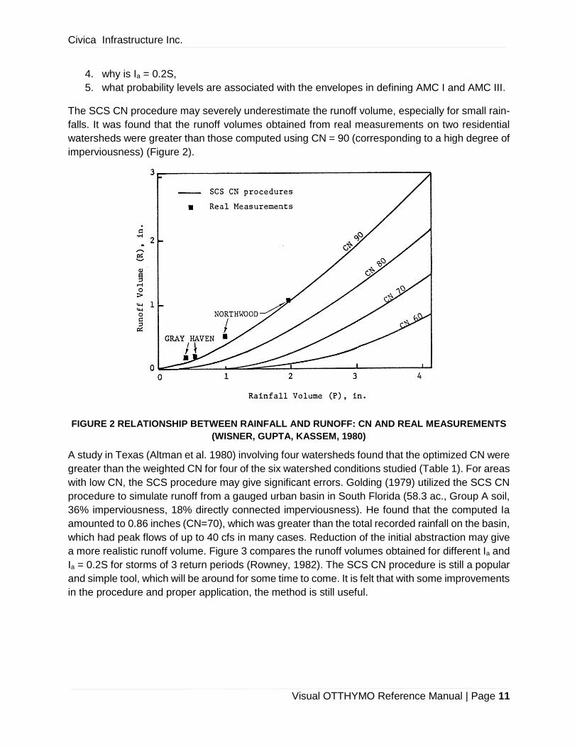
The SCS CN procedure may severely underestimate the runoff volume, especially for small rain-
falls. It was found that the runoff volumes obtained from real measurements on two residential
watersheds were greater than those computed using CN = 90 (corresponding to a high degree of
imperviousness) (Figure 2).
FIGURE 2 RELATIONSHIP BETWEEN RAINFALL AND RUNOFF: CN AND REAL MEASUREMENTS
(WISNER, GUPTA, KASSEM, 1980)
A study in Texas (Altman et al. 1980) involving four watersheds found that the optimized CN were
greater than the weighted CN for four of the six watershed conditions studied (Table 1). For areas
with low CN, the SCS procedure may give significant errors. Golding (1979) utilized the SCS CN
procedure to simulate runoff from a gauged urban basin in South Florida (58.3 ac., Group A soil,
36% imperviousness, 18% directly connected imperviousness). He found that the computed Ia
amounted to 0.86 inches (CN=70), which was greater than the total recorded rainfall on the basin,
which had peak flows of up to 40 cfs in many cases. Reduction of the initial abstraction may give
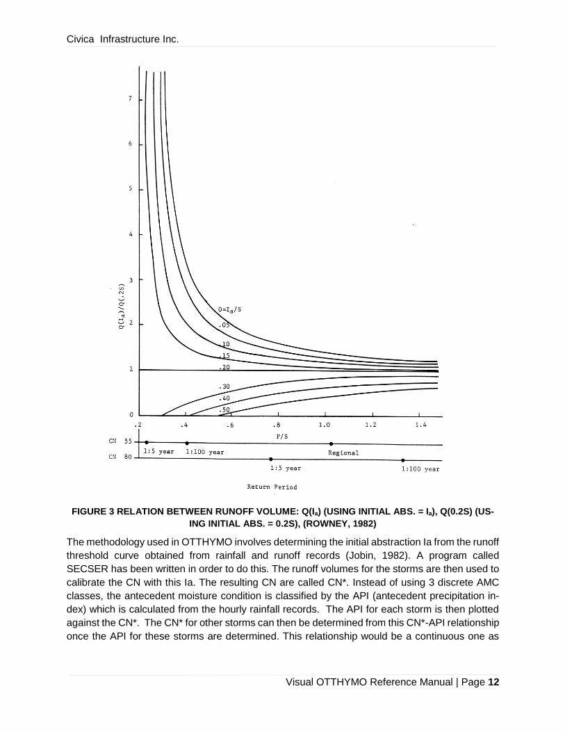
a more realistic runoff volume. Figure 3 compares the runoff volumes obtained for different Ia and
Ia = 0.2S for storms of 3 return periods (Rowney, 1982). The SCS CN procedure is still a popular
and simple tool, which will be around for some time to come. It is felt that with some improvements
in the procedure and proper application, the method is still useful.
Civica Infrastructure Inc.
Visual OTTHYMO Reference Manual | Page 12
FIGURE 3 RELATION BETWEEN RUNOFF VOLUME: Q(Ia) (USING INITIAL ABS. = Ia), Q(0.2S) (US-
ING INITIAL ABS. = 0.2S), (ROWNEY, 1982)
The methodology used in OTTHYMO involves determining the initial abstraction Ia from the runoff
threshold curve obtained from rainfall and runoff records (Jobin, 1982). A program called
SECSER has been written in order to do this. The runoff volumes for the storms are then used to
calibrate the CN with this Ia. The resulting CN are called CN*. Instead of using 3 discrete AMC
classes, the antecedent moisture condition is classified by the API (antecedent precipitation in-
dex) which is calculated from the hourly rainfall records. The API for each storm is then plotted
against the CN*. The CN* for other storms can then be determined from this CN*-API relationship
once the API for these storms are determined. This relationship would be a continuous one as
Civica Infrastructure Inc.
Visual OTTHYMO Reference Manual | Page 13
compared to the 3 discrete classes used in SCS. It also would not require the definition of a
standard reference moisture condition.
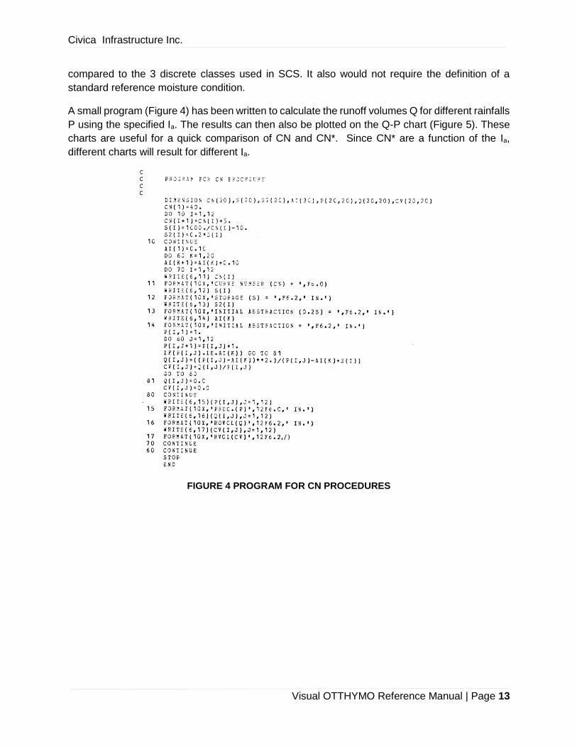
A small program (Figure 4) has been written to calculate the runoff volumes Q for different rainfalls
P using the specified Ia. The results can then also be plotted on the Q-P chart (Figure 5). These
charts are useful for a quick comparison of CN and CN*. Since CN* are a function of the Ia,
different charts will result for different Ia.
FIGURE 4 PROGRAM FOR CN PROCEDURES
Civica Infrastructure Inc.
Visual OTTHYMO Reference Manual | Page 14
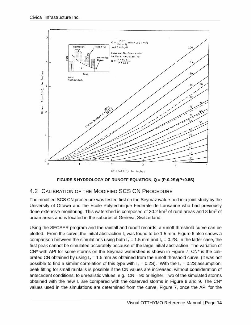
FIGURE 5 HYDROLOGY OF RUNOFF EQUATION, Q = (P-0.2S)/(P+0.8S)
4.2 CALIBRATION OF THE MODIFIED SCS CN PROCEDURE
The modified SCS CN procedure was tested first on the Seymaz watershed in a joint study by the
University of Ottawa and the Ecole Polytechnique Federale de Lausanne who had previously
done extensive monitoring. This watershed is composed of 30.2 km2 of rural areas and 8 km2 of
urban areas and is located in the suburbs of Geneva, Switzerland.
Using the SECSER program and the rainfall and runoff records, a runoff threshold curve can be
plotted. From the curve, the initial abstraction Ia was found to be 1.5 mm. Figure 6 also shows a
comparison between the simulations using both Ia = 1.5 mm and Ia = 0.2S. In the latter case, the
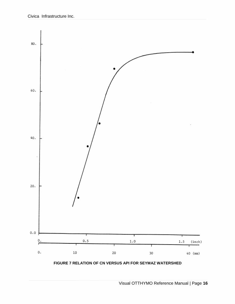
first peak cannot be simulated accurately because of the large initial abstraction. The variation of
CN* with API for some storms on the Seymaz watershed is shown in Figure 7. CN* is the cali-
brated CN obtained by using Ia = 1.5 mm as obtained from the runoff threshold curve. (It was not
possible to find a similar correlation of this type with Ia = 0.2S). With the Ia = 0.2S assumption,
peak fitting for small rainfalls is possible if the CN values are increased, without consideration of
antecedent conditions, to unrealistic values, e.g., CN = 90 or higher. Two of the simulated storms
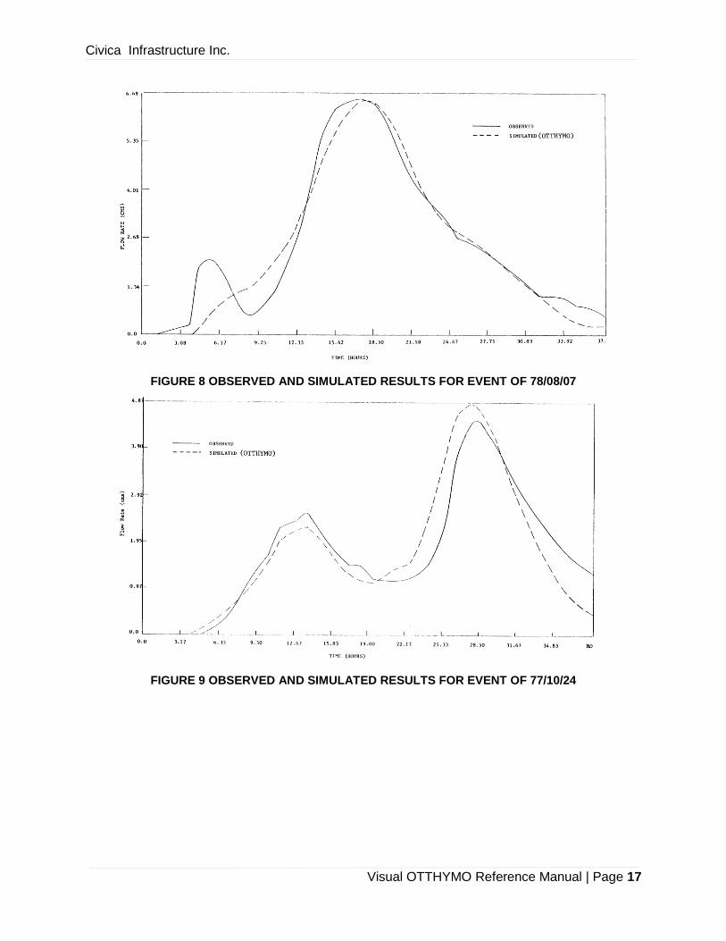
obtained with the new Ia are compared with the observed storms in Figure 8 and 9. The CN*
values used in the simulations are determined from the curve, Figure 7, once the API for the
Civica Infrastructure Inc.
Visual OTTHYMO Reference Manual | Page 15
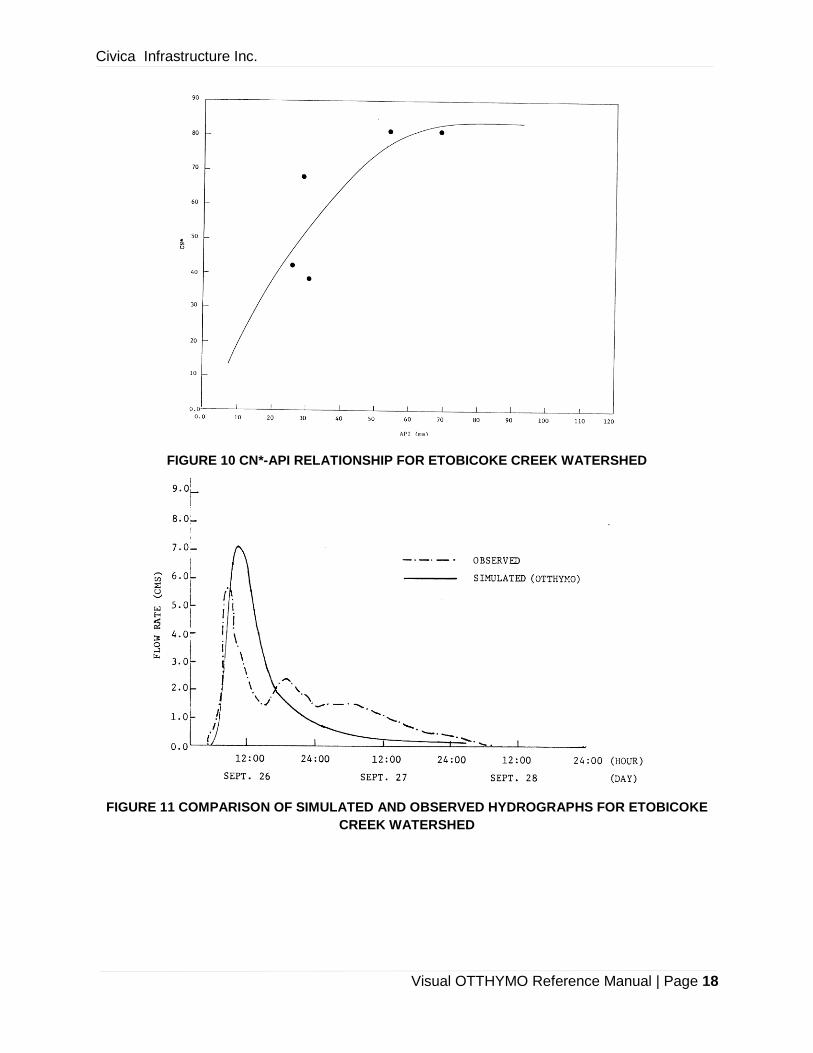
storms are obtained. A similar CN*-API relationship has been determined for the Etobicoke Creek
watershed (Figure 10) in Metro Toronto. One of the typical comparisons between simulated and
observed storms is shown in Figure 11.
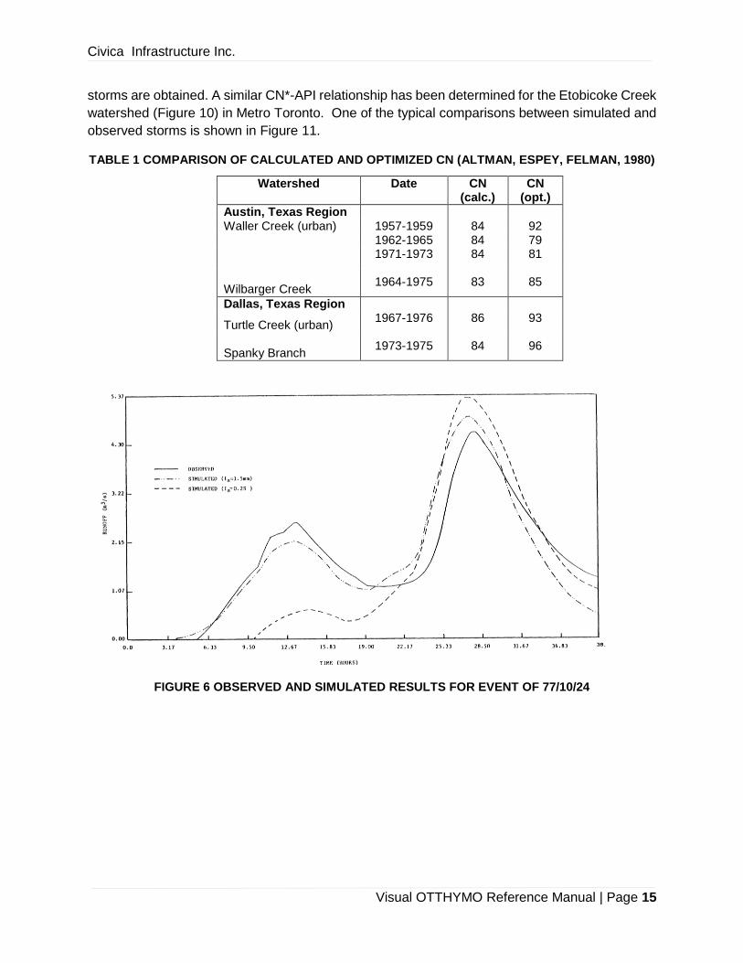
TABLE 1 COMPARISON OF CALCULATED AND OPTIMIZED CN (ALTMAN, ESPEY, FELMAN, 1980)
Watershed Date CN (calc.)
CN (opt.)
Austin, Texas Region Waller Creek (urban) 1957-1959 84 92
1962-1965 84 79
1971-1973 84 81
Wilbarger Creek 1964-1975 83 85
Dallas, Texas Region
Turtle Creek (urban) 1967-1976 86 93
Spanky Branch 1973-1975 84 96
FIGURE 6 OBSERVED AND SIMULATED RESULTS FOR EVENT OF 77/10/24
Civica Infrastructure Inc.
Visual OTTHYMO Reference Manual | Page 16
FIGURE 7 RELATION OF CN VERSUS API FOR SEYMAZ WATERSHED
Civica Infrastructure Inc.
Visual OTTHYMO Reference Manual | Page 17
FIGURE 8 OBSERVED AND SIMULATED RESULTS FOR EVENT OF 78/08/07
FIGURE 9 OBSERVED AND SIMULATED RESULTS FOR EVENT OF 77/10/24
Civica Infrastructure Inc.
Visual OTTHYMO Reference Manual | Page 18
FIGURE 10 CN*-API RELATIONSHIP FOR ETOBICOKE CREEK WATERSHED
FIGURE 11 COMPARISON OF SIMULATED AND OBSERVED HYDROGRAPHS FOR ETOBICOKE
CREEK WATERSHED

Civica Infrastructure Inc.
Visual OTTHYMO Reference Manual | Page 19
4.3 INFILTRATION PROCEDURES IN STANDHYD
4.3.1 HORTON'S EQUATION
For pervious areas, there are two options for calculating the infiltration losses. The first option is
Horton's equation where the infiltration capacity rate is an exponential function of time, which
decays to a constant rate. It is written as follows:
𝑓𝑡 = 𝑓𝑐 + (𝑓𝑜 − 𝑓𝑐)𝑒−𝛼𝑡 (9)
where:
𝑓𝑡 = the infiltration capacity rate (in/hr or mm/hr) at time t;
𝑓𝑜 = the initial infiltration capacity rate (in/hr or mm/hr);
𝑓𝑐 = the final infiltration capacity rate (in/hr or mm/hr);
𝛼 = the decay rate (1/hr).
The equation is only satisfactory for the condition that the rainfall intensity is higher than the infil-
tration capacity rate. To overcome this problem, the cumulative form of the equation can be used.
It has the advantage that the infiltration rate becomes a function of the amount of water accumu-
lated into the soil.
𝐹 = ∫ 𝑓𝑡𝑑𝑡𝑡
0
= 𝑓𝑐 +(𝑓𝑜 − 𝑓𝑐)
𝛼(1 − 𝑒−𝛼𝑡) (10)
where 𝐹 is the cumulative infiltration volume, at time 𝑡.
The average infiltration capacity rate during the next time step is
𝑓�̅� =𝐹(𝑡 + ∆𝑡) − 𝐹(𝑡)
∆𝑡 (11)
In order to determine the actual infiltration rate f, the average infiltration capacity rate is then
compared with the average rainfall intensity i during the time period ∆𝑡.
If
𝑓 =𝑓�̅� 𝑖 > 𝑓�̅�
𝑖 𝑖 < 𝑓�̅� (12)
then the calculation proceeds to the next time step with the cumulative infiltration volume at
𝐹(𝑡 + ∆𝑡). If f = i, then the actual cumulative infiltration would be
𝐹𝑎𝑐𝑡. = 𝐹(𝑡) + 𝑖∆𝑡 (13)
where
𝐹𝑎𝑐𝑡. < 𝐹(𝑡 + ∆𝑡) (14)
Civica Infrastructure Inc.
Visual OTTHYMO Reference Manual | Page 20
The new time 𝑡1, which would correspond to the cumulative infiltration 𝐹𝑎𝑐𝑡., is determined by
means of an iterative process. The calculation then continues from this point for the next time
step.
The antecedent moisture condition can be represented by the water, F, accumulated into the soil
before the start of the storm. F can be directly specified as input. The other infiltration parameters
also need to be specified.
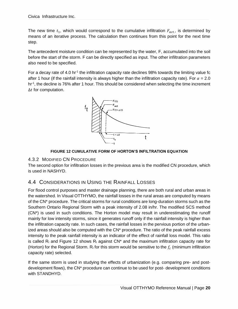
For a decay rate of 4.0 hr-1 the infiltration capacity rate declines 98% towards the limiting value fc
after 1 hour (if the rainfall intensity is always higher than the infiltration capacity rate). For 𝛼 = 2.0
hr-1, the decline is 76% after 1 hour. This should be considered when selecting the time increment
∆𝑡 for computation.
FIGURE 12 CUMULATIVE FORM OF HORTON’S INFILTRATION EQUATION
4.3.2 MODIFIED CN PROCEDURE
The second option for infiltration losses in the previous area is the modified CN procedure, which
is used in NASHYD.
4.4 CONSIDERATIONS IN USING THE RAINFALL LOSSES
For flood control purposes and master drainage planning, there are both rural and urban areas in
the watershed. In Visual OTTHYMO, the rainfall losses in the rural areas are computed by means
of the CN* procedure. The critical storms for rural conditions are long-duration storms such as the
Southern Ontario Regional Storm with a peak intensity of 2.08 in/hr. The modified SCS method
(CN*) is used in such conditions. The Horton model may result in underestimating the runoff
mainly for low intensity storms, since it generates runoff only if the rainfall intensity is higher than
the infiltration capacity rate. In such cases, the rainfall losses in the pervious portion of the urban-
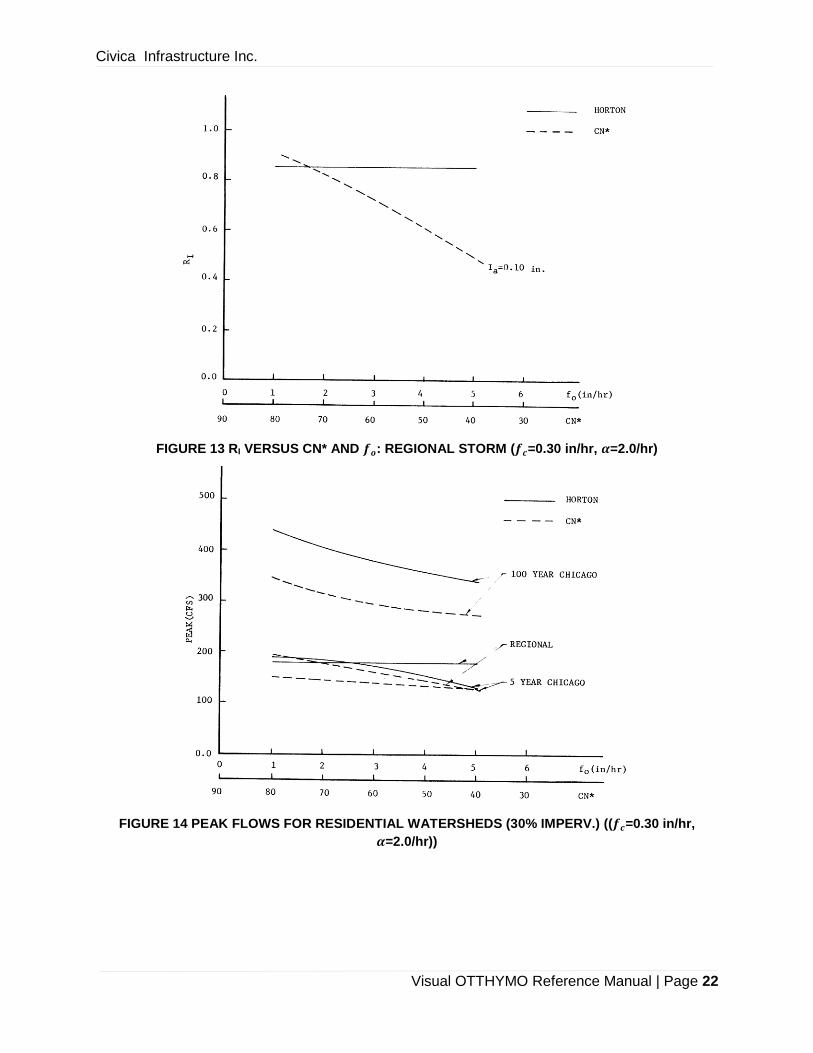
ized areas should also be computed with the CN* procedure. The ratio of the peak rainfall excess
intensity to the peak rainfall intensity is an indicator of the effect of rainfall loss model. This ratio
is called RI and Figure 12 shows RI against CN* and the maximum infiltration capacity rate for
(Horton) for the Regional Storm. RI for this storm would be sensitive to the 𝑓𝑐 (minimum infiltration
capacity rate) selected.
If the same storm is used in studying the effects of urbanization (e.g. comparing pre- and post-
development flows), the CN* procedure can continue to be used for post- development conditions
with STANDHYD.

Civica Infrastructure Inc.
Visual OTTHYMO Reference Manual | Page 21
For design purposes under urban conditions, however, the critical storms are the short- duration,
high intensity storms such as the Chicago-type storms. Here Horton's procedure is preferred be-
cause it is more sensitive to the storm intensity and in general results in higher peak flows than
the CN* procedure. This is shown in Figure 13 for a residential watershed (30% imperviousness)
for three storms, the 5-year, 100-year Chicago and the Regional storms.
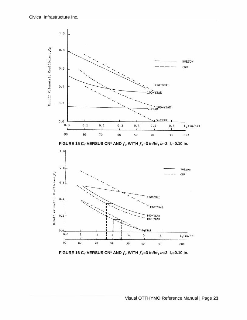
A series of numerical experiments have been done to find a range of values in which the Horton
and CN* procedures would give the same runoff volumes. The runoff volumetric coefficient Cv
was calculated for different combinations of 𝑓𝑜, 𝑓𝑐 and values (Horton) and CN* values (with Ia =
0.10 in). The range of values tested were 1.0 to 5.0 in/hr for 𝑓𝑜, 0.10 to 0.50 in/hr for 𝑓𝑐 and 2.0/hr
and 4.14/hr for 𝛼 (decay constant). The results are shown in Figure 14 and 15. The peak flows
for a 121-acre residential watershed for the values shown in Figure 15 are plotted in Figure 13. It
is observed that equivalent Cv does not mean that the corresponding peak flows are equivalent.
It is also found that total runoff for the Regional storm is more sensitive to 𝑓𝑐 while for the Chicago
storms they are more sensitive to 𝑓𝑜. There is no range of values for which the Cv are matched
for all three storms. Figure 14 shows that the Cv for the Regional storm can be matched by varying
𝑓𝑐 and Figure 15 show that the Cv for the Chicago storms can be matched by varying 𝑓𝑜.
These results show that for consistency the selection of infiltration parameters should consider
the characteristics of the soil and also those of the storm. Tables given in literature in which infil-
tration parameters like 𝑓𝑜, 𝑓𝑐 and CN are given in terms of soil groups A, B, C, D alone may not
give consistent results.
If data is available and the CN*-API relationship has already been derived during the planning
stage, the CN* procedure can also be used for design purposes. The use of the CN* procedure
with design storms is discussed in the section on design storms. This will result in compatibility
between the planning and the design stages for the watershed.
Civica Infrastructure Inc.
Visual OTTHYMO Reference Manual | Page 22
FIGURE 13 RI VERSUS CN* AND 𝒇𝒐: REGIONAL STORM (𝒇𝒄=0.30 in/hr, 𝜶=2.0/hr)
FIGURE 14 PEAK FLOWS FOR RESIDENTIAL WATERSHEDS (30% IMPERV.) ((𝒇𝒄=0.30 in/hr,
𝜶=2.0/hr))
Civica Infrastructure Inc.
Visual OTTHYMO Reference Manual | Page 23
FIGURE 15 CV VERSUS CN* AND 𝒇𝒄 WITH 𝒇𝒐=3 in/hr, 𝜶=2, Ia=0.10 in.
FIGURE 16 CV VERSUS CN* AND 𝒇𝒄 WITH 𝒇𝒐=3 in/hr, 𝜶=2, Ia=0.10 in.
Civica Infrastructure Inc.
Visual OTTHYMO Reference Manual | Page 24
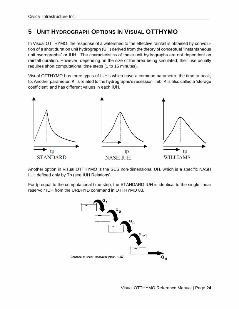
5 UNIT HYDROGRAPH OPTIONS IN VISUAL OTTHYMO
In Visual OTTHYMO, the response of a watershed to the effective rainfall is obtained by convolu-
tion of a short duration unit hydrograph (UH) derived from the theory of conceptual “instantaneous
unit hydrographs” or IUH. The characteristics of these unit hydrographs are not dependent on
rainfall duration. However, depending on the size of the area being simulated, their use usually
requires short computational time steps (1 to 15 minutes).
Visual OTTHYMO has three types of IUH's which have a common parameter, the time to peak,
tp. Another parameter, K, is related to the hydrographs’s recession limb. K is also called a ‘storage
coefficient’ and has different values in each IUH.
Another option in Visual OTTHYMO is the SCS non-dimensional UH, which is a specific NASH
IUH defined only by Tp (see IUH Relations).
For tp equal to the computational time step, the STANDARD IUH is identical to the single linear
reservoir IUH from the URBHYD command in OTTHYMO 83.

Civica Infrastructure Inc.
Visual OTTHYMO Reference Manual | Page 25
5.1 IUH RELATIONS
TYPE OF IUH RELATION REMARKS
STANDARD
𝑞
𝑞𝑝𝑒𝑎𝑘= 𝑡/𝑇𝑝 for 𝑡 < 𝑇𝑝
𝑞
𝑞𝑝𝑒𝑎𝑘= 𝑒−(𝑡−𝑇𝑝)/𝑘 for 𝑡 > 𝑇𝑝
For Tp = DT (the computa-tional time step) the STAND-ARD IUH becomes the UR-BHYD IUH from OTTHYMO 83.
NASH 𝑞
𝑞𝑝𝑒𝑎𝑘
= (𝑡/𝑇𝑝)(𝑁−1)
𝑒(1−𝑁)(
𝑡𝑇𝑝
−1)
N = Tp / k + 1 N is also the “number of reser-voirs”
WILLIAMS
for 𝑡 < 𝑡𝑜
𝑞
𝑞𝑝𝑒𝑎𝑘
= (𝑡/𝑇𝑝)(𝑁−1)
𝑒(1−𝑁)(
𝑡𝑇𝑝
−1)
and, 𝑞𝑝𝑒𝑎𝑘 = [1/(𝐾𝑛Γ(𝑁))]𝑒(1−𝑁)(𝑁 − 1)(𝑁−1)
for 𝑡𝑜 < 𝑡 < 𝑡1 (𝑤ℎ𝑒𝑟𝑒 𝑡1 = 𝑡𝑜 + 2𝑘)
𝑞
𝑞𝑜
= 𝑒(𝑡𝑜−𝑡)/𝑘
for 𝑡1 < 𝑡
𝑞
𝑞𝑜
= 𝑒(𝑡1−𝑡)/3𝑘
Calibration recommended.
Where 𝑡𝑜 is the inflection point
after the peak; 𝐾𝑛 is the storage
coefficient of each reservoir; 𝑁
is the number of reservoirs, and
Γ(𝑁) is the gamma function.
SCS Is the NASH IUH with N = 5
Civica Infrastructure Inc.
Visual OTTHYMO Reference Manual | Page 26
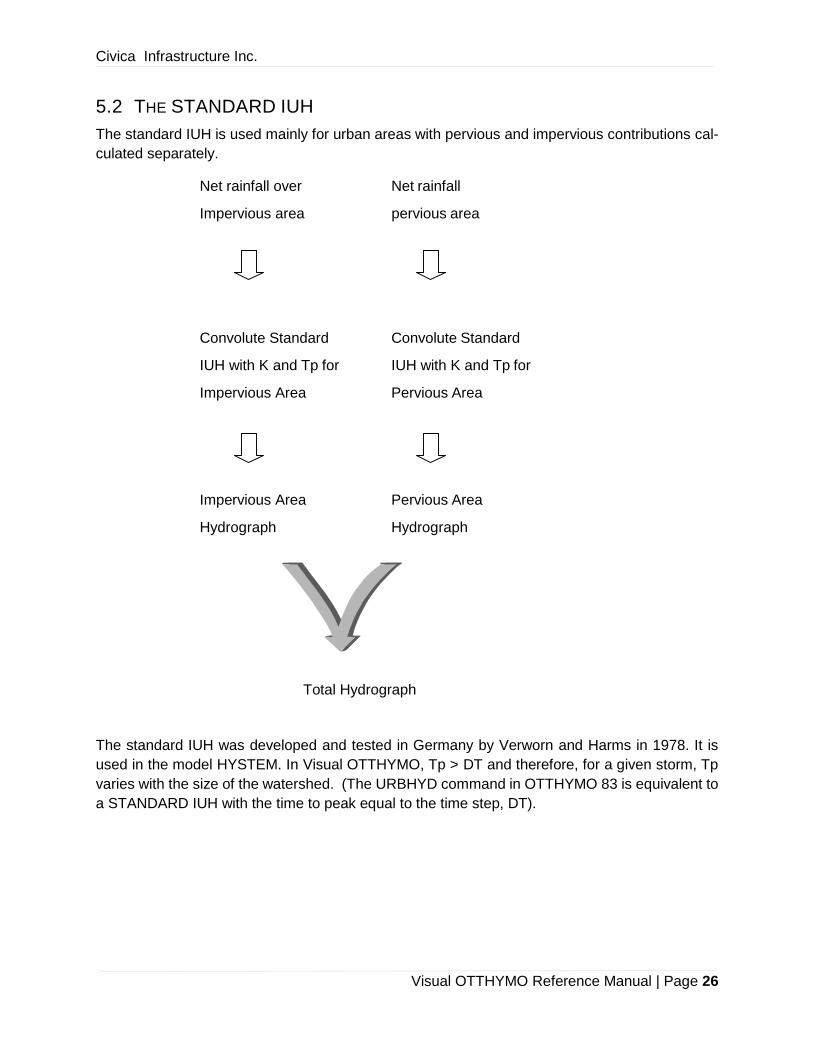
5.2 THE STANDARD IUH
The standard IUH is used mainly for urban areas with pervious and impervious contributions cal-
culated separately.
Net rainfall over Net rainfall
Impervious area pervious area
Convolute Standard Convolute Standard
IUH with K and Tp for IUH with K and Tp for
Impervious Area Pervious Area
Impervious Area Pervious Area
Hydrograph Hydrograph
Total Hydrograph
The standard IUH was developed and tested in Germany by Verworn and Harms in 1978. It is
used in the model HYSTEM. In Visual OTTHYMO, Tp > DT and therefore, for a given storm, Tp
varies with the size of the watershed. (The URBHYD command in OTTHYMO 83 is equivalent to
a STANDARD IUH with the time to peak equal to the time step, DT).
Civica Infrastructure Inc.
Visual OTTHYMO Reference Manual | Page 27
A relation derived from overland routing by the kinematic wave method (Peterson and Altera)
gives the storage coefficient, K. This relation is close to the relation by Neumann used in HYS-
TEM.
𝐾 = 𝐶𝐿0.6 ∙ 𝑛0.6
𝑖0.4 ∙ 𝑠0.3
where:
𝐿= an equivalent flow length which requires calibration. A default value for impervious areas
obtained from 𝐴 = 1.5𝐿2 where 𝐴 is the watershed area, was frequently tested with meas-
urements. For pervious areas, the default value is 𝐿 = 40 m, representing an average
travel length on inter-spaced green areas.
𝑛= the roughness coefficient. Testing shows that adequate results are obtained it 𝑛 = 0.013
for impervious areas and 𝑛 = 0.25 for pervious areas.
𝑖 = the dominant rainfall intensity (maximum average intensity during K).
𝑠 = the characteristic slope in m/m.
𝐶 =a constant (0.00775 for L in feet, i in inches/hour).
The STANDHYD command is based on analysis of comparisons with measurements and practi-
cal applications. In STANDHYD, the dominant rainfall intensity is averaged over the duration of
K. Since K varies with rainfall intensity this IUH varies from one rainfall to the other, the STAND-
ARD IUH is a quasi-linear model.
For the impervious area, the time to peak, Tp, in the STANDARD IUH of Visual OTTHYMO is
equal to the storage coefficient, K. For the pervious areas, fragmented in backyards and con-
nected to storm sewers, Tp is equal to K pervious + K impervious, at time of convolution, Tp is
rounded to the nearest multiple of the time step, DT.
In the STANDHYD command, the pervious hydrograph and the impervious hydrograph have, in
general, different Tp values. There is also a lag between the peak discharge of the total hydro-
graph and the end of the peak rainfall intensity.
For watersheds with large estate lots and semi-urban areas with relatively large pervious compo-
nents, it is recommended to simulate two component hydrographs:
a) The first, an equivalent smaller urban area can be simulated with STANDHYD.
b) The remaining area which is only (or mostly) pervious, can be simulated with NASHYD.
The equivalent urban area and the imperviousness of this area (e.g., say 30 %) satisfy the follow-
ing rule of thumb:
𝐸𝑞𝑢𝑖𝑣𝑎𝑙𝑒𝑛𝑡 𝐴𝑢𝑟𝑏𝑎𝑛 ∗ 0.30 = 𝐴𝑡𝑜𝑡𝑎𝑙 ∗ (𝑅𝑒𝑎𝑙 𝑖𝑚𝑝𝑒𝑟𝑣𝑖𝑜𝑢𝑠𝑛𝑒𝑠𝑠)
Fore very large urban areas (> 200 hectares), STANDHYD requires calibration.
Civica Infrastructure Inc.
Visual OTTHYMO Reference Manual | Page 28
5.3 THE NASH IUH (NASHYD)
This linear IUH is used mainly for rural areas. With Nash, the peak discharge increases with N
and decreases with Tp. Measurements in Ontario and in Switzerland indicate that an average of
3 number of linear reservoirs may be appropriate.
The time to peak, Tp, is obtained from the time of concentration, Tc:
Tp = (N-1)/N Tc where, N, is the number of linear reservoirs
Tp = 0.67 Tc
In general, the time of concentration, Tc, can be determined using one of three methods:
1. Empirical formulas (only recommended if they are based on regional verifications).
2. Velocity methods, Tc = 3 (Li/Vi). The overland velocities are determined with an SCS
graph, and channel velocities can be determined from Manning’s equation.
3. Kinematic wave method (which accounts for the rainfall intensity).
The NASHYD command is used for non-homogeneous areas, and in the case of SCS abstraction
methods, uses a weighted average of CN. Comparisons with measurements show a better per-
formance if the response from the pervious and impervious areas are simulated separately.
Fore very large urban areas (> 200 hectares), NASHYD requires calibration.
Furthermore, if the response time of an urban watershed is increased by significant channel stor-
age, this effect must be simulated by channel routing (unless Tp is calibrated).
5.4 THE SCS IUH (SCSHYD)
The shape of the SCS UH is obtained from the NASH relation, with N=5. This value is greater
than the one determined from studies in Ontario, Switzerland, and the United Kingdom. It is,
however, conservative if the time to peak is correct.
The SCS non-dimensional unit hydrograph is used by SCS abstraction methods for both rural and
urban areas. Comparisons with measurements show that even if Tp, Ia, and CN* are calibrated,
the proper shape of the hydrograph is not always generated.
The 1986 SCS TR-55 publication indicates the following limitations:
1. Hydrographs obtained by this method are not developed for comparisons with measure-
ments.
2. The method should only be used in cases where runoff is greater than 12.5 mm.
3. The lag formula given in previous SCS publications is no longer recommended (it may
underestimate the peak flow).
The SCS methods apply the non-dimensional UH in conjunction the SCS CN method with the
assumption that Ia = 0.2 x S. Although this may overestimate the rainfall losses, it was maintained
in the SCS command for special agency requests.
Civica Infrastructure Inc.
Visual OTTHYMO Reference Manual | Page 29
It is recommended the to determine Tc with the velocity method:
Tc = 3 (Li/Vi)
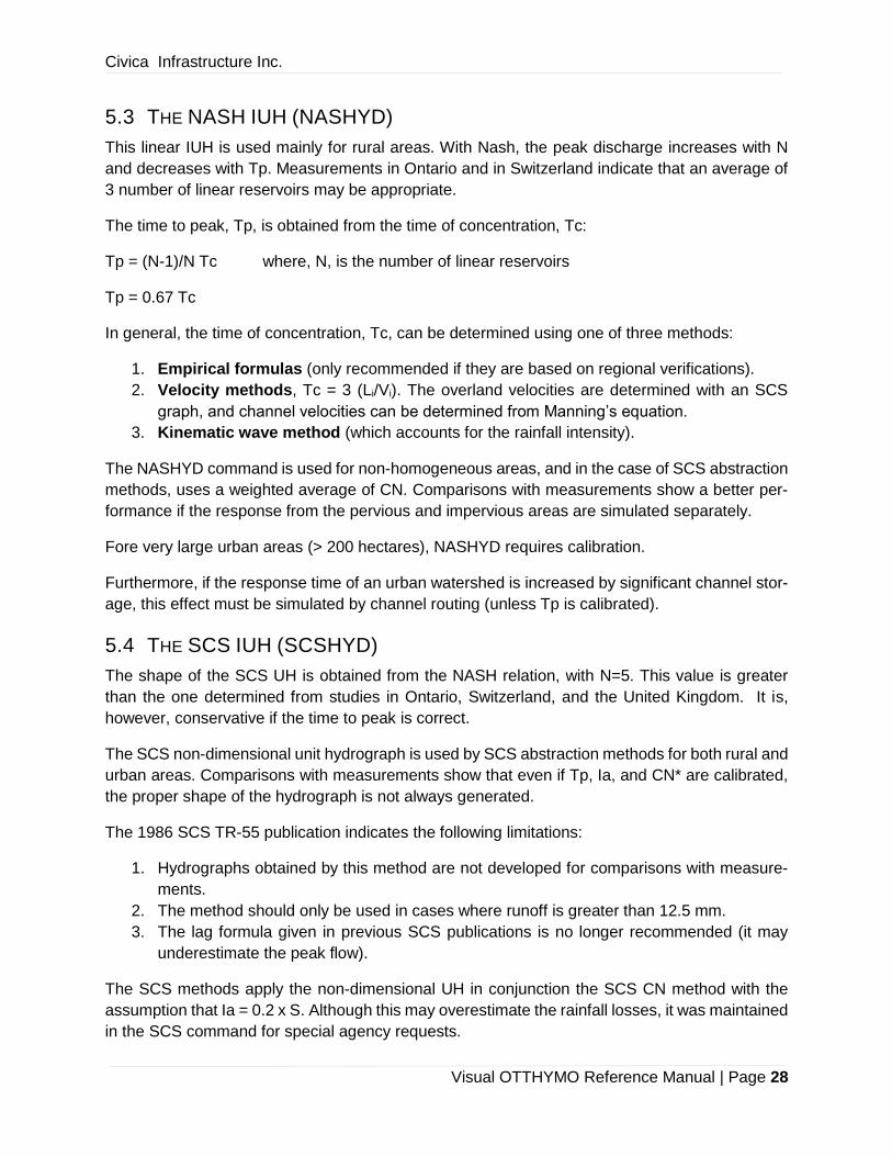
5.5 THE WILLIAMS IUH
The method is recommended for rural watersheds where observations indicate a long hydrograph
recession limbs. The Williams formula for Tp is not recommended in Ontario as it has been shown
to give significant errors.
FIGURE 17 WILLIAMS IUH
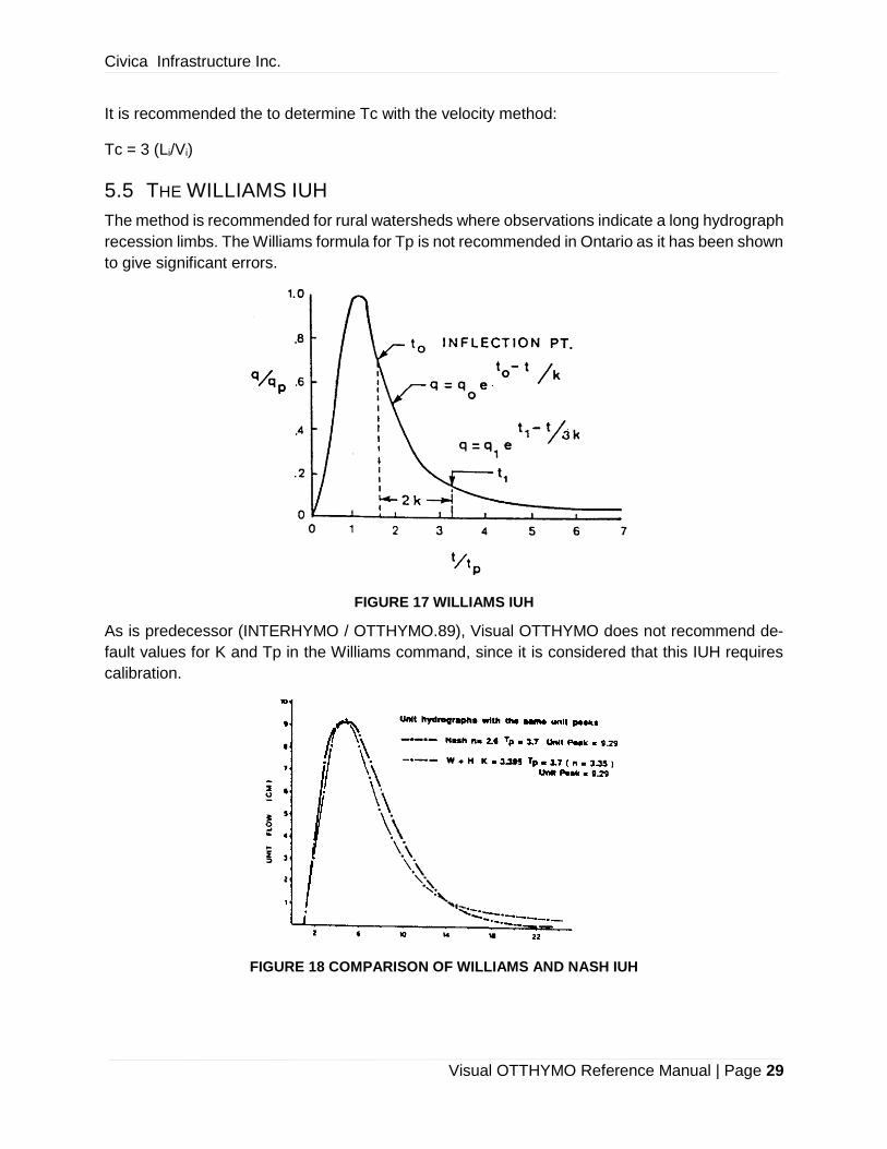
As is predecessor (INTERHYMO / OTTHYMO.89), Visual OTTHYMO does not recommend de-
fault values for K and Tp in the Williams command, since it is considered that this IUH requires
calibration.
FIGURE 18 COMPARISON OF WILLIAMS AND NASH IUH
Civica Infrastructure Inc.
Visual OTTHYMO Reference Manual | Page 30
5.6 USE OF IUH’S FOR I/I SIMULATION AND BASEFLOW (DWF)
Visual OTTHYMO can be used to simulate the Infiltration/Inflow into sanitary sewers or combined
sewers. The four types or rainfall-induced infiltration/inflow are:
1. Fast responses from directly connected impervious areas.
2. Rapid responses from grassed areas in combined sewers systems.
3. Semi-rapid responses from weeping tiles.
4. Slow responses from cracked pipes and leaking joints in the sewers.
Visual OTTHYMO can simulate these responses during a single event by adding individual re-
sponse hydrographs from each type of contributions within the same area. The first three re-
sponses can be simulated with the quasi-linear instantaneous Unit Hydrograph (STANDHYD)
while the fourth, slow response, can be simulated with the NASH unit hydrograph.
Baseflow can be super-imposed to account for the domestic sewage contributions during wet
conditions.
5.7 UNIT HYDROGRAPH OPTIONS FOR RURAL AREAS
For computation of flows from rural watersheds, the subroutines NASHYD, WILHYD or SCSHYD
(NASHYD with N=5) can be used. The rainfall excess distribution is obtained by means of a mod-
ified CN procedure, which is then convoluted with the unit hydrograph obtained by means of the
Nash model (NASHYD) or the Williams and Hann unit hydrograph (WILHYD).
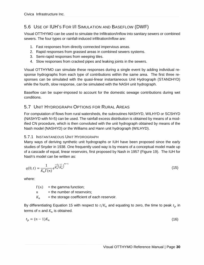
5.7.1 INSTANTANEOUS UNIT HYDROGRAPH
Many ways of deriving synthetic unit hydrographs or IUH have been proposed since the early
studies of Snyder in 1938. One frequently used way is by means of a conceptual model made up
of a cascade of equal, linear reservoirs, first proposed by Nash in 1957 (Figure 19). The IUH for
Nash's model can be written as:
𝑞(0, 𝑡) =1
𝐾𝑛Γ(𝑛)𝑒
−𝑡𝐾𝑛
(𝑡
𝐾𝑛)
𝑛−1
(15)
where:
Γ(𝑛) = the gamma function;
𝑛 = the number of reservoirs;
𝐾𝑛 = the storage coefficient of each reservoir.
By differentiating Equation 15 with respect to 𝑡/𝐾𝑛 and equating to zero, the time to peak 𝑡𝑝 in
terms of 𝑛 and 𝐾𝑛 is obtained.
𝑡𝑝 = (𝑛 − 1)𝐾𝑛 (16)
Civica Infrastructure Inc.
Visual OTTHYMO Reference Manual | Page 31
The peak flow then becomes
𝑞𝑝 = 1
𝐾𝑛𝛤(𝑛)𝑒1−𝑛(𝑛 − 1)𝑛−1 (17)
By substituting Equations 16 and 17 in Equation 15, the 2-parameter gamma equation is obtained
𝑞 = 𝑞𝑝 (𝑡
𝑡𝑝
)
(𝑛−1)
𝑒(1−𝑛)(
𝑡𝑡𝑝
−1) (18)
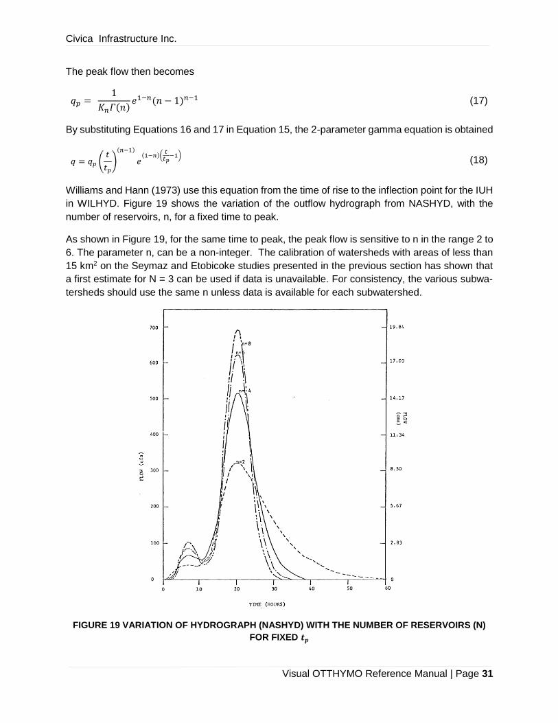
Williams and Hann (1973) use this equation from the time of rise to the inflection point for the IUH
in WILHYD. Figure 19 shows the variation of the outflow hydrograph from NASHYD, with the
number of reservoirs, n, for a fixed time to peak.
As shown in Figure 19, for the same time to peak, the peak flow is sensitive to n in the range 2 to
6. The parameter n, can be a non-integer. The calibration of watersheds with areas of less than
15 km2 on the Seymaz and Etobicoke studies presented in the previous section has shown that
a first estimate for N = 3 can be used if data is unavailable. For consistency, the various subwa-
tersheds should use the same n unless data is available for each subwatershed.
FIGURE 19 VARIATION OF HYDROGRAPH (NASHYD) WITH THE NUMBER OF RESERVOIRS (N)
FOR FIXED 𝒕𝒑
Civica Infrastructure Inc.
Visual OTTHYMO Reference Manual | Page 32
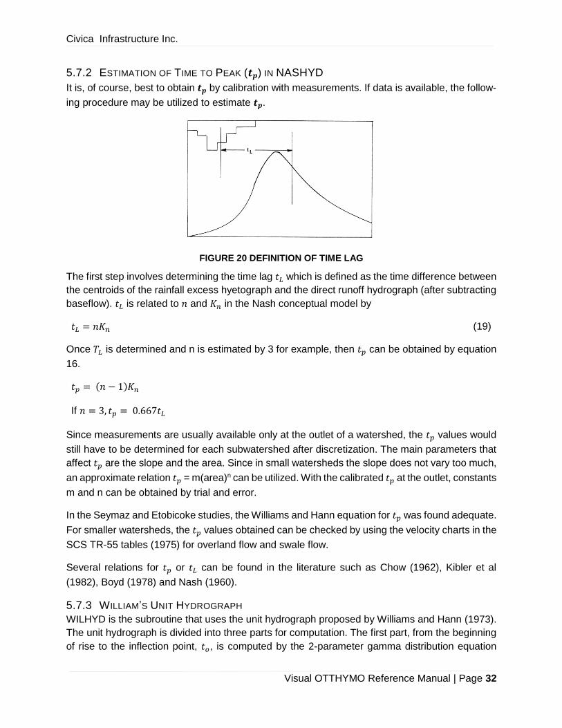
5.7.2 ESTIMATION OF TIME TO PEAK (𝒕𝒑) IN NASHYD
It is, of course, best to obtain 𝒕𝒑 by calibration with measurements. If data is available, the follow-
ing procedure may be utilized to estimate 𝒕𝒑.
FIGURE 20 DEFINITION OF TIME LAG
The first step involves determining the time lag 𝑡𝐿 which is defined as the time difference between
the centroids of the rainfall excess hyetograph and the direct runoff hydrograph (after subtracting
baseflow). 𝑡𝐿 is related to 𝑛 and 𝐾𝑛 in the Nash conceptual model by
𝑡𝐿 = 𝑛𝐾𝑛 (19)
Once 𝑇𝐿 is determined and n is estimated by 3 for example, then 𝑡𝑝 can be obtained by equation
16.
𝑡𝑝 = (𝑛 − 1)𝐾𝑛
If 𝑛 = 3, 𝑡𝑝 = 0.667𝑡𝐿
Since measurements are usually available only at the outlet of a watershed, the 𝑡𝑝 values would
still have to be determined for each subwatershed after discretization. The main parameters that
affect 𝑡𝑝 are the slope and the area. Since in small watersheds the slope does not vary too much,
an approximate relation 𝑡𝑝 = m(area)n can be utilized. With the calibrated 𝑡𝑝 at the outlet, constants
m and n can be obtained by trial and error.
In the Seymaz and Etobicoke studies, the Williams and Hann equation for 𝑡𝑝 was found adequate.
For smaller watersheds, the 𝑡𝑝 values obtained can be checked by using the velocity charts in the
SCS TR-55 tables (1975) for overland flow and swale flow.
Several relations for 𝑡𝑝 or 𝑡𝐿 can be found in the literature such as Chow (1962), Kibler et al
(1982), Boyd (1978) and Nash (1960).
5.7.3 WILLIAM’S UNIT HYDROGRAPH
WILHYD is the subroutine that uses the unit hydrograph proposed by Williams and Hann (1973).
The unit hydrograph is divided into three parts for computation. The first part, from the beginning
of rise to the inflection point, 𝑡𝑜, is computed by the 2-parameter gamma distribution equation

Civica Infrastructure Inc.
Visual OTTHYMO Reference Manual | Page 33
(Equation 18). The second part from the inflection point, 𝑡𝑜 to 𝑡1 where 𝑡1 = 𝑡𝑜 + 2𝐾, is computed
by
𝑞 = 𝑞𝑜𝑒𝑡𝑜−𝑡
𝐾 (20)
The third part from 𝑡1 onwards is computed by
𝑞 = 𝑞1𝑒𝑡1−𝑡3𝐾 (21)
n is computed as a function of 𝐾/𝑡𝑝 and 𝑞𝑝 is a function of 𝑛 and 𝑡𝑝. Therefore only 2 parameters,
𝐾 and 𝑡𝑝 are necessary to compute the entire unit hydrograph. Empirical relations have been
derived for 𝐾 and 𝑡𝑝 (Williams 1977) based on Southern U.S. watersheds. These relations may
not be applicable in other areas.
𝐾 = 16.1𝐴0.24𝑆−0.84 (22)
𝑡𝑝 = 6.54𝐴0.39𝑆−0.50 (23)
where:
𝐾 = the recession constant (hr);
𝑡𝑝 = the time to peak (hr);
𝐴 = the watershed area (sq.miles); and
𝑆 = the difference in elevation in feet, divided by flood plain distance in miles, between
watershed outlet and most distant point on the watershed.
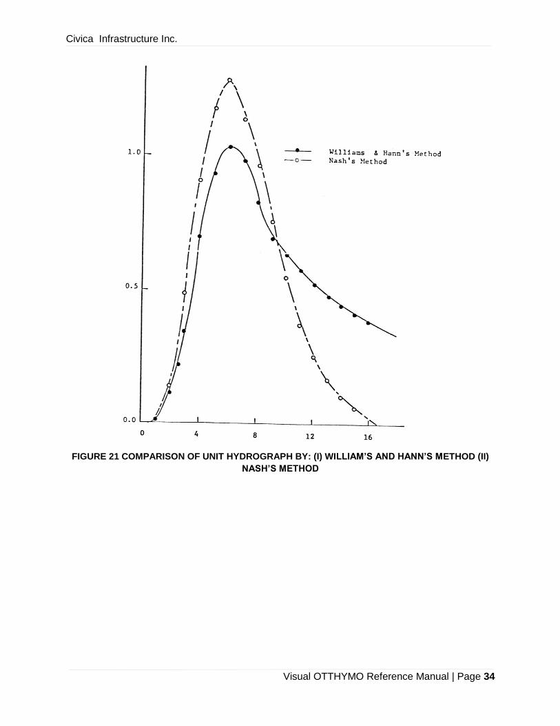
The unit hydrograph in WILHYD has a longer recession tail than that in NASHYD and a smaller
peak. It can therefore be used in those watersheds where the recession limb is longer.
A comparison of the two unit hydrographs is shown in Figure 21.
Civica Infrastructure Inc.
Visual OTTHYMO Reference Manual | Page 34
FIGURE 21 COMPARISON OF UNIT HYDROGRAPH BY: (I) WILLIAM’S AND HANN’S METHOD (II)
NASH’S METHOD
Civica Infrastructure Inc.
Visual OTTHYMO Reference Manual | Page 35
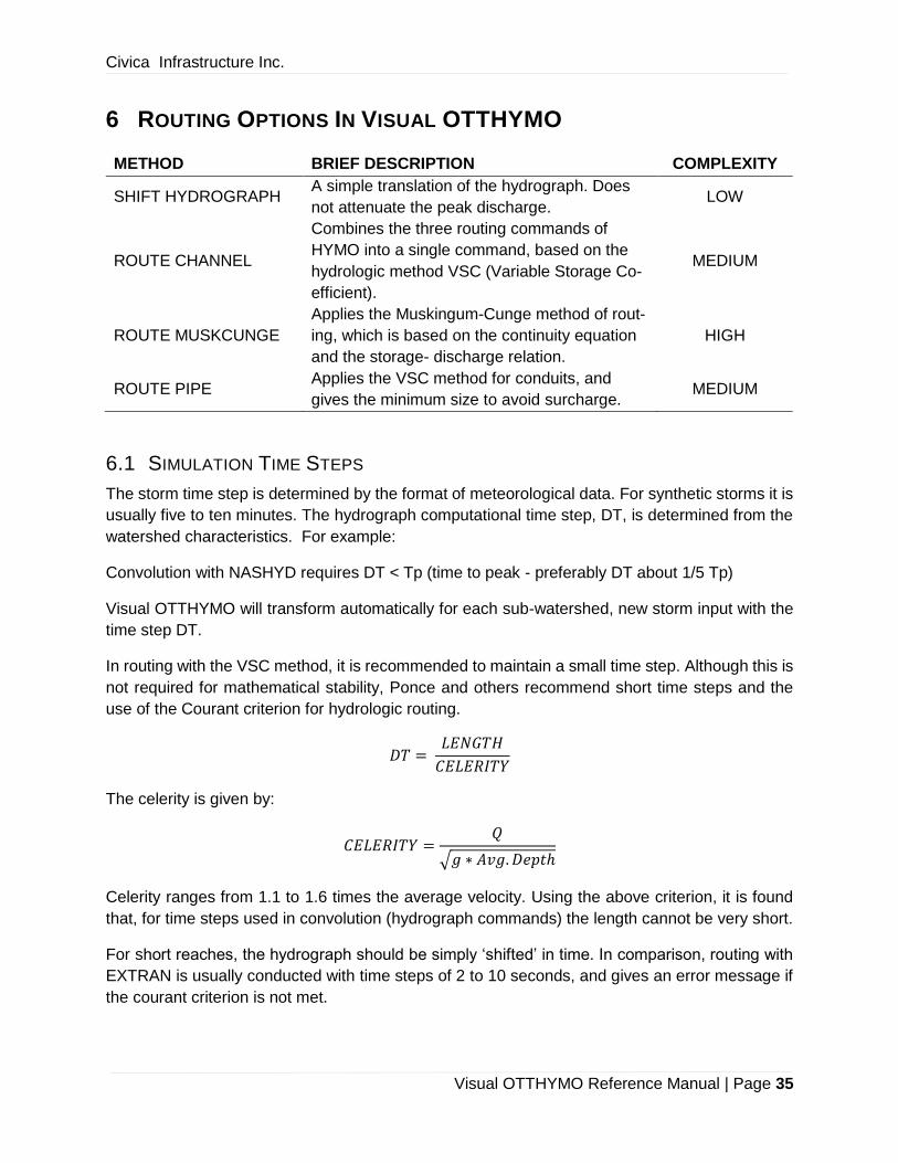
6 ROUTING OPTIONS IN VISUAL OTTHYMO
METHOD BRIEF DESCRIPTION COMPLEXITY
SHIFT HYDROGRAPH A simple translation of the hydrograph. Does
not attenuate the peak discharge. LOW
ROUTE CHANNEL
Combines the three routing commands of
HYMO into a single command, based on the
hydrologic method VSC (Variable Storage Co-
efficient).
MEDIUM
ROUTE MUSKCUNGE
Applies the Muskingum-Cunge method of rout-
ing, which is based on the continuity equation
and the storage- discharge relation.
HIGH
ROUTE PIPE Applies the VSC method for conduits, and
gives the minimum size to avoid surcharge. MEDIUM
6.1 SIMULATION TIME STEPS
The storm time step is determined by the format of meteorological data. For synthetic storms it is
usually five to ten minutes. The hydrograph computational time step, DT, is determined from the
watershed characteristics. For example:
Convolution with NASHYD requires DT < Tp (time to peak - preferably DT about 1/5 Tp)
Visual OTTHYMO will transform automatically for each sub-watershed, new storm input with the
time step DT.
In routing with the VSC method, it is recommended to maintain a small time step. Although this is
not required for mathematical stability, Ponce and others recommend short time steps and the
use of the Courant criterion for hydrologic routing.
𝐷𝑇 = 𝐿𝐸𝑁𝐺𝑇𝐻
𝐶𝐸𝐿𝐸𝑅𝐼𝑇𝑌
The celerity is given by:
𝐶𝐸𝐿𝐸𝑅𝐼𝑇𝑌 =𝑄
√𝑔 ∗ 𝐴𝑣𝑔. 𝐷𝑒𝑝𝑡ℎ
Celerity ranges from 1.1 to 1.6 times the average velocity. Using the above criterion, it is found
that, for time steps used in convolution (hydrograph commands) the length cannot be very short.
For short reaches, the hydrograph should be simply ‘shifted’ in time. In comparison, routing with
EXTRAN is usually conducted with time steps of 2 to 10 seconds, and gives an error message if
the courant criterion is not met.
Civica Infrastructure Inc.
Visual OTTHYMO Reference Manual | Page 36
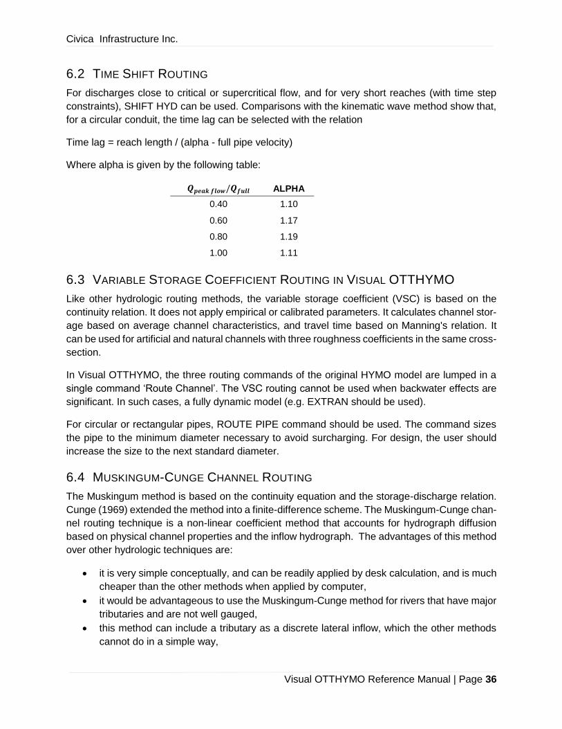
6.2 TIME SHIFT ROUTING
For discharges close to critical or supercritical flow, and for very short reaches (with time step
constraints), SHIFT HYD can be used. Comparisons with the kinematic wave method show that,
for a circular conduit, the time lag can be selected with the relation
Time lag = reach length / (alpha - full pipe velocity)
Where alpha is given by the following table:
𝑸𝒑𝒆𝒂𝒌 𝒇𝒍𝒐𝒘/𝑸𝒇𝒖𝒍𝒍 ALPHA
0.40 1.10
0.60 1.17
0.80 1.19
1.00 1.11
6.3 VARIABLE STORAGE COEFFICIENT ROUTING IN VISUAL OTTHYMO
Like other hydrologic routing methods, the variable storage coefficient (VSC) is based on the
continuity relation. It does not apply empirical or calibrated parameters. It calculates channel stor-
age based on average channel characteristics, and travel time based on Manning's relation. It
can be used for artificial and natural channels with three roughness coefficients in the same cross-
section.
In Visual OTTHYMO, the three routing commands of the original HYMO model are lumped in a
single command ‘Route Channel’. The VSC routing cannot be used when backwater effects are
significant. In such cases, a fully dynamic model (e.g. EXTRAN should be used).
For circular or rectangular pipes, ROUTE PIPE command should be used. The command sizes
the pipe to the minimum diameter necessary to avoid surcharging. For design, the user should
increase the size to the next standard diameter.
6.4 MUSKINGUM-CUNGE CHANNEL ROUTING
The Muskingum method is based on the continuity equation and the storage-discharge relation.
Cunge (1969) extended the method into a finite-difference scheme. The Muskingum-Cunge chan-
nel routing technique is a non-linear coefficient method that accounts for hydrograph diffusion
based on physical channel properties and the inflow hydrograph. The advantages of this method
over other hydrologic techniques are:
• it is very simple conceptually, and can be readily applied by desk calculation, and is much
cheaper than the other methods when applied by computer,
• it would be advantageous to use the Muskingum-Cunge method for rivers that have major
tributaries and are not well gauged,
• this method can include a tributary as a discrete lateral inflow, which the other methods
cannot do in a simple way,

Civica Infrastructure Inc.
Visual OTTHYMO Reference Manual | Page 37
• the hydrologic approach greatly improves computational efficiency and speed, and re-
duces the amount and detail of field data traditionally needed for hydraulic routing,
• the parameters of the model are physical based, the scheme is stable with properly se-
lected coefficients,
• the method has been shown to compare well against the full unsteady flow equations over
a wide range of flow situations,
• it produces consistent results in that the results are reproducible with varying grid solution,
• it is comparable to the diffusion wave routing,
• it is largely independent of the time and space intervals when these are selected within
the spatial and temporal resolution criteria,
The major limitations are:
• it cannot account for backwater effects,
• the method begins to diverge from the full unsteady flow solution when very rapidly rising
hydrographs are routed through flat channel sections,
• a disadvantage with the Muskingum-Cunge method arises when there is a disturbance
such as a tide affecting the flow in the river upstream of the downstream boundary,
• it does not accurately predict the shape of the discharge hydrograph at the downstream
boundary when there are large variations in the kinematic wave speed, such as due to the
inundation of a large flood plain.
6.4.1 BASIC FLOW EQUATIONS
The outflow hydrograph at the downstream end is calculated using the following formula.
𝑄𝑗+1𝑛+1 = 𝐶1𝑄𝑗
𝑛 + 𝐶2𝑄𝑗𝑛+1 + 𝐶3𝑄𝑗+1
𝑛 + 𝐶4 (24)
where:
𝐶1 =𝐾𝑥 +
Δ𝑡2
𝐷
(25)
𝐶2 =
Δ𝑡2 − 𝐾𝑥
𝐷
(26)
𝐶3 =𝐾(1 − 𝑥) −
Δ𝑡2
𝐷
(27)
𝐶4 =𝑞∆𝑡∆𝑥
𝐷
(28)
𝐷 = 𝐾(1 − 𝑥) +∆𝑡
2
(29)

Civica Infrastructure Inc.
Visual OTTHYMO Reference Manual | Page 38
Where:
𝑄 = discharge
𝐾 = travel time in seconds
𝑥 = weighting factor, 0 <= 𝑥 <= 0.5
∆𝑥 = subreach length
∆𝑡 = time interval q = lateral flow
c = wave celerity
The parameters of 𝐾 and 𝑥 are expressed as follows (Cunge, 1969 and Ponce, 1978):
𝐾 =∆𝑥
𝑐 (30)
𝑥 =1
2 (1 −𝑄
𝑐𝐵𝑆∆𝑥) (31)
where:
𝐵 = top width
𝑆 = the channel slope.
6.4.2 SOLUTION OF FLOW EQUATIONS
The outflow hydrograph is iterative and is calculated based on equation 24, the routing coefficients
(𝐶1, 𝐶2, 𝐶3, 𝐶4) are re-calculated for every distance step ∆𝑥 and calculation time step ∆𝑡.
Numerical Stability
∆𝑡 and ∆𝑥 are chosen internally by the model for accuracy and stability.
∆𝑡 is selected as the smallest of the following 3 rules:
1. the user defined computation interval, DT,
2. the time of rise of the hydrograph divided by 20,
3. the travel time of the channel reach.
The model checks the difference between the computational time interval (DT) and the time in-
crement of the inflow hydrograph (SDT). If DT is less than SDT, the inflow hydrograph will be
interpolated. The calculation time step must be equal or less than the inflow hydrograph SDT.
A computational space increment ∆𝑥 can be equal to the length of the entire routing reach or to a
fraction of that length. It is initially selected as the entire reach length. If the size of this space
increment does not meet the accuracy criteria for flow routing given by Ponce and Theurer (1982),
it is re-evaluated by subdividing the length of the routing reach into even subreaches that produce
∆𝑥’s that satisfy the accuracy criteria.
Civica Infrastructure Inc.
Visual OTTHYMO Reference Manual | Page 39
where,
∆𝑥 =1
2(𝑐∆𝑡 +
𝑄
𝐵𝑆𝐶) (32)
where,
𝑄 = 𝑄𝐵 + 0.5 ∗ (𝑄𝑝 − 𝑄𝐵) (33)
𝑄𝐵 = baseflow from the inflow hydrograph
𝑄𝑝 = peak flow from the inflow hydrograph
The Courant (𝐶) number can be defined as:
𝐶 =𝑐∆𝑡
∆𝑥 (34)
Main and overbank channel portions are separated and modelled as two independent channels.
Right and left overbanks are combined into a single overbank channel.
Momentum at the flow interface between the two channel portions is neglected, and the hydraulic
flow characteristics are determined separately, for each channel portion. At the upstream end of
a space increment, the total inflow discharge is divided into main channel and overbank flow
components. Each are then routed independently, using the previously described routing scheme.
The flow redistribution between the main and overbank channels is based on Manning's equation.
6.4.3 DATA REQUIREMENTS
Data required for the Muskingum-Cunge method are as followings:
• channel length
• main channel bed slope
• floodplain bed slope
• beta parameter (a function of the storage-discharge curve)
• channel cross section data
• number of cross section segments
• Manning roughness coefficient
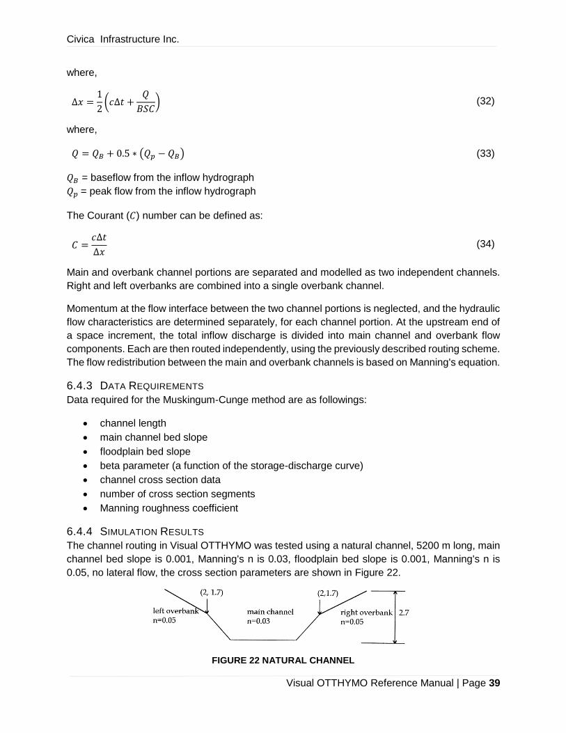
6.4.4 SIMULATION RESULTS
The channel routing in Visual OTTHYMO was tested using a natural channel, 5200 m long, main
channel bed slope is 0.001, Manning's n is 0.03, floodplain bed slope is 0.001, Manning's n is
0.05, no lateral flow, the cross section parameters are shown in Figure 22.
FIGURE 22 NATURAL CHANNEL
Civica Infrastructure Inc.
Visual OTTHYMO Reference Manual | Page 40
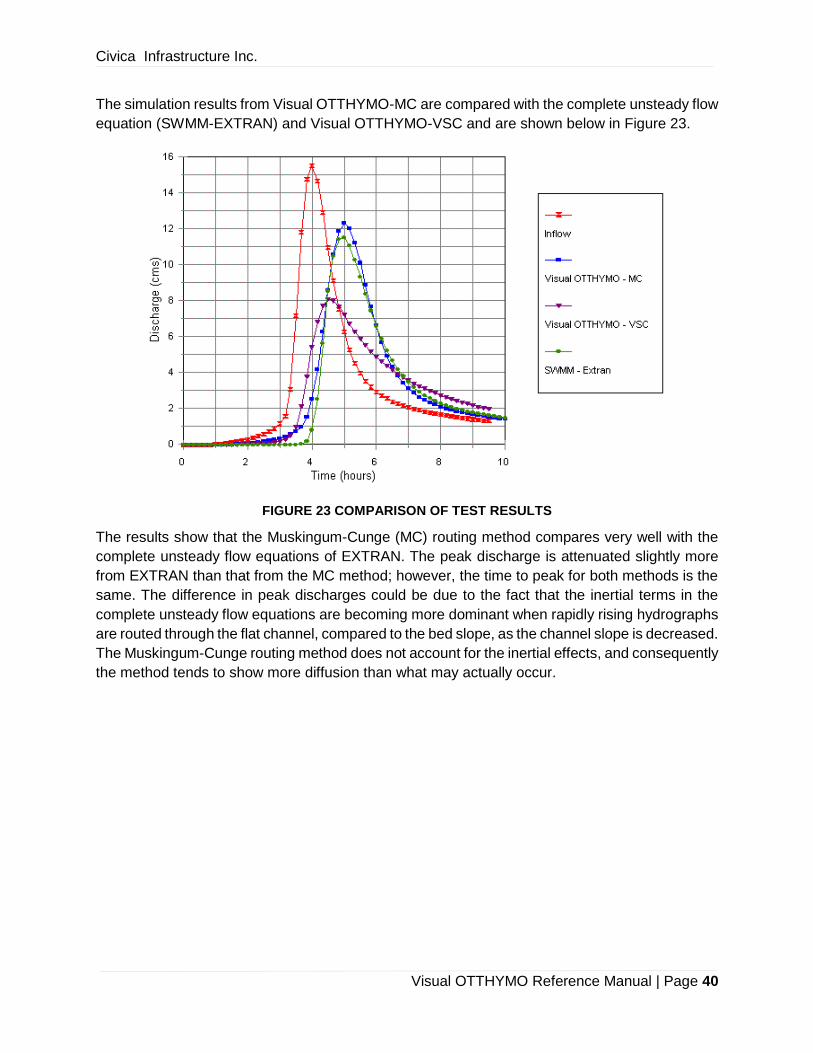
The simulation results from Visual OTTHYMO-MC are compared with the complete unsteady flow
equation (SWMM-EXTRAN) and Visual OTTHYMO-VSC and are shown below in Figure 23.
FIGURE 23 COMPARISON OF TEST RESULTS
The results show that the Muskingum-Cunge (MC) routing method compares very well with the
complete unsteady flow equations of EXTRAN. The peak discharge is attenuated slightly more
from EXTRAN than that from the MC method; however, the time to peak for both methods is the
same. The difference in peak discharges could be due to the fact that the inertial terms in the
complete unsteady flow equations are becoming more dominant when rapidly rising hydrographs
are routed through the flat channel, compared to the bed slope, as the channel slope is decreased.
The Muskingum-Cunge routing method does not account for the inertial effects, and consequently
the method tends to show more diffusion than what may actually occur.

Civica Infrastructure Inc.
Visual OTTHYMO Reference Manual | Page 41
7 DESIGN STORMS FOR STORMWATER MANAGEMENT STUDIES
Flow simulation for urban drainage studies is mostly done with one-event simulation models. The
single event models determine flows produced by a single storm event. Continuous simulation
models require rainfall data over a continuous period for the desired length of analysis. A fre-
quency analysis is then conducted on the peak flows so that a flow of a desired return period may
be found.
The flow with a single event model may be found by using a series of selected historical events
or by using a ‘design storm’. The historical storm series may be selected using a continuous
simulation program or by analyzing a rainfall record using a selection criteria. Each event in the
selected series is then run through the event simulation model. The generated peak flows are
then analyzed to determine their return period.
Design storms or model storms are single event rainfalls that are assumed to produce flows of a
desired return period. They are of two types; synthetic design storms and historic design storms.
Synthetic design storms are storms developed from intensity- duration-frequency (IDF) curves.
Historic design storms are large single storm events; usually containing the maximum precipita-
tion on record. In southern Ontario, hurricane Hazel is used as an historic design storm. In this
text only synthetic design storms are examined.
Each design storm has a unique temporal variation of intensity. Two general methods are used
to determine the hyetograph shape. The first method derives the storm pattern based on an IDF
curve. The design storms using only an IDF curve are the Uniform design storm, the Composite
design storm and the Chicago design storm. The second method obtains the temporal structure
of the design storm from an analysis of historic storm events. These are the U.S. Soil Conserva-
tion Service (SCS) 24-hour design storm, the SCS 6-hour design storm, the Illinois State Water
Survey (ISWS) design storm, the Atmospheric Environment Service (AES) design storm, the
Flood Studies Report (FSR) design storm, the Pilgrim and Cordery design storm and the Yen and
Chow design storm. Design storms that are not discussed are the Sifalda design storm, the Ham-
burg design storm and the Desordes (French) design storm. A more detailed description of each
design storm is contained in the Design Storm Profiles section of this document. Table 2 summa-
rizes the main characteristics of these design storms.
Each of the design storms has a different hyetograph shape. Storm hyetographs were constructed
and compared for some of the design storms. A five year return period was selected and the
storm volumes were obtained from the Bloor Street station (Toronto) IDF curve. The duration of
the storms are not all the same, for this reason the storm volumes are different. The storm hyet-
ographs for the Uniform, Composite, Chicago, SCS 24-hr., ISWS, AES, FSR, and Yen and Chow
design storms are shown in Figures 24 and 25.
Civica Infrastructure Inc.
Visual OTTHYMO Reference Manual | Page 42
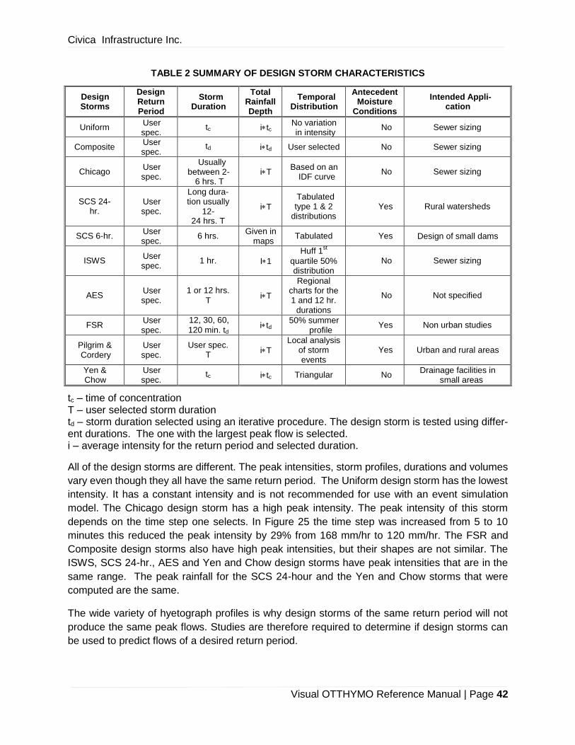
TABLE 2 SUMMARY OF DESIGN STORM CHARACTERISTICS
Design Storms
Design Return Period
Storm Duration
Total Rainfall Depth
Temporal Distribution
Antecedent Moisture
Conditions
Intended Appli-cation
Uniform User spec.
tc itc No variation in intensity
No Sewer sizing
Composite User spec.
td itd User selected No Sewer sizing
Chicago User spec.
Usually between 2-
6 hrs. T iT
Based on an IDF curve
No Sewer sizing
SCS 24- hr.
User spec.
Long dura-tion usually
12- 24 hrs. T
iT
Tabulated type 1 & 2
distributions Yes Rural watersheds
SCS 6-hr. User spec.
6 hrs. Given in
maps Tabulated Yes Design of small dams
ISWS User spec.
1 hr. I1
Huff 1st
quartile 50% distribution
No Sewer sizing
AES User spec.
1 or 12 hrs.
T iT
Regional charts for the 1 and 12 hr.
durations
No Not specified
FSR User spec.
12, 30, 60,
120 min. td itd
50% summer profile
Yes Non urban studies
Pilgrim & Cordery
User spec.
User spec. T
iT
Local analysis of storm events
Yes Urban and rural areas
Yen & Chow
User spec.
tc itc Triangular No Drainage facilities in
small areas
tc – time of concentration T – user selected storm duration td – storm duration selected using an iterative procedure. The design storm is tested using differ-ent durations. The one with the largest peak flow is selected. i – average intensity for the return period and selected duration.
All of the design storms are different. The peak intensities, storm profiles, durations and volumes
vary even though they all have the same return period. The Uniform design storm has the lowest
intensity. It has a constant intensity and is not recommended for use with an event simulation
model. The Chicago design storm has a high peak intensity. The peak intensity of this storm
depends on the time step one selects. In Figure 25 the time step was increased from 5 to 10
minutes this reduced the peak intensity by 29% from 168 mm/hr to 120 mm/hr. The FSR and
Composite design storms also have high peak intensities, but their shapes are not similar. The
ISWS, SCS 24-hr., AES and Yen and Chow design storms have peak intensities that are in the
same range. The peak rainfall for the SCS 24-hour and the Yen and Chow storms that were
computed are the same.
The wide variety of hyetograph profiles is why design storms of the same return period will not
produce the same peak flows. Studies are therefore required to determine if design storms can
be used to predict flows of a desired return period.

Civica Infrastructure Inc.
Visual OTTHYMO Reference Manual | Page 43
A review of previous studies showed that there is contradictory opinion regarding the use of de-
sign storms. Marsalek (1978) does not recommend the use of design storms while the results of
Arnell (1982) and Watson (1981) suggest that design storms should be used. Other researchers
have concluded that further studies are required.
Those who recommend the use of design storms consider that their advantages outweigh the
shortcomings. The advantages of using design storms are that:
1. They are an inexpensive procedure for obtaining flows of a desired return period.
2. If properly selected they give conservative results for peak flows and volumes.
3. They are widely used in current engineering practice.
Some of the disadvantages of design storms are that:
1. The runoff frequency is assumed to be the same as the rainfall frequency. This equiva-
lence of return period has not been shown to be true.
2. The rainfall volume is not the rainfall volume of real storm events.
3. Using IDF relationships to obtain a design storm hyetograph may be incorrect.
A study was conducted using IMPSWM procedures to test two design storms commonly used by
Canadian engineers. The uniform design storm was not tested because of its low, unrealistic
intensity. The Chicago and the SCS 24-hr design storms were selected for the study. The AES
design storm could have been used but the 30% profile with a 1-hour duration gives peak flow
results close the Chicago storm and historical storm flows (Wisner and Gupta, 1980). With a 12-
hour duration the AES 50% profile gives results similar to the SCS 24-hr. design storm. The third
chapter contains the results that compare the Chicago and the SCS 24-hr design storms. The
methodology can be used for any other design storm by a municipality.
FIGURE 24 COMPARISON OF DESIGN STORMS

Civica Infrastructure Inc.
Visual OTTHYMO Reference Manual | Page 44
FIGURE 25 COMPARISON OF DESIGN STORMS
7.1 METHODOLOGY OF DESIGN STORMS
The researchers comparing peak flows from design storms and historical storms used different
catchments and different simulation programs. A comparison of the peak flow frequency results
for the Chicago design storm is presented first in this chapter. The results for this storm are sum-
marized in Table 3.
A study conducted in the IMPSWM program is also presented here. The methodology used to
compare the Chicago and SCS 24-hr design storms with the historical storms is given in the
second section of the chapter.
7.1.1 RESULTS FOR THE CHICAGO DESIGN STORM
J.F. McLarens Ltd. (1978) has conducted studies on catchments in Edmonton and Winnipeg.
They found that the ratio of the Chicago storm peak flow to the flows from an historic storm series
ranged between 1.0 and 1.2. It was recommended that the Chicago design storm be used for
urban drainage design.
Marsalek (1979) developed a Chicago design storm for the Burlington area. He found that the
peak flows produced from the Chicago design storm are 80% larger than those produced from
historical storm events. He also found that the peak flow was attenuated as the catchment size
increased. The peak flow increased as the catchment imperviousness increased but the peak
flow overestimation remains at approximately 80%. These results were analyzed in the IMPSWM
program by Wisner and Gupta (1980). They concluded that discrepancies can be reduced if the

Civica Infrastructure Inc.
Visual OTTHYMO Reference Manual | Page 45
peak intensity of the design storms are reduced to values in agreement with measured peak in-
tensities.
Watson (1980) compared the peak flows obtained from the Chicago design storm and historical
storm events. A 2-hr. duration and a non-dimensional time to peak of 0.28 is used to develop the
Chicago storm. The rainfall data is discretized at 5 min. intervals.
TABLE 3 SUMMARY OF RESULTS FROM PERVIOUS STUDIES (AVERAGE PERCENTAGE DIFFER-
ENCE BETWEEN THE CHICAGO DESIGN STORM AND HISTORICAL STORM FLOWS)
Study Catchment Chicago Design Storm
Arnell (1980) Bergsjon Linkoping 1 Linkoping 2
-2.2% 10.3% 6.0%
Marsalek (1979) Burlington (area 26 ha, imp. 30%)
80.0%
Watson (1980) Pinetown Kew
2.0% -5.0%
Watson found that on the Pinetown catchment the peak flows from the Chicago storm agreed
closely with those from the historical storms. The agreement for the Kew catchment was not quite
as good. The peak flow is slightly underestimated. It is within 95% confidence interval bands of
the historical storms, though. The Kew catchment is less impervious than the Pinetown catch-
ment; therefore, it is more sensitive to antecedent moisture conditions.
Arnell (1982) used a Chicago design storm with a 4-hr duration. The non-dimensional time to
peak, r, is 0.43 if the return period is less than 1 year. If the return period is greater than 1 year, r
is 0.35. The Chicago storm is developed with a step size of one minute.
Arnell found that the Chicago design storm overestimated the peak flow by approximately 5%. On
the Bergsjon catchment, the peak flow is underestimated by 2.2%. On the Linkoping 1 and
Linkoping 2 catchments the flow is overestimated by 10.3% and 6% respectively. The Bergsjon
catchment was the smallest of the three catchments. The Chicago storm produces peak flows
almost identical to the historical storms on this catchment.
With the exception of Marsalek (1979), the estimation of peak flow produced by the Chicago storm
gave acceptable results compared with that produced by historical storms. Differences range from
a 2% underestimation to an 10% overestimation of peak flow.
Watson recommended that the Chicago design storm be used for peak flow design. Arnell also
found that the deviation of the Chicago Storm peak flow values from the historical storm peak flow
values are not large. He concludes that the Chicago Storm should overestimate peak flows be-
cause of the way it is developed. He does not recommend the use of the Chicago design storm
because of the large overestimation of peak flow Marsalek found.

Civica Infrastructure Inc.
Visual OTTHYMO Reference Manual | Page 46
7.2 METHODOLOGY FOR COMPARING DESIGN STORMS AND A HISTORICAL
STORM SERIES
7.2.1 RAINFALL INPUT
The rainfall inputs used with the event simulation models were a historical storm series and two
design storms. The historical storm series was selected from the Bloor Street station rainfall rec-
ord. A criteria was selected based on the storm volume and intensity so that approximately one
storm event for each year in the record was chosen. This results in some years having more than
one event and other years having no events. The selected events were then discretized to ten
minute time intervals. A summary of the storm events and their characteristics is given in Table
4.
The SCS 24-hour and Chicago design storms were compared with the historical storm series.
The design storms were developed from the Bloor Street station IDF curves for return periods of
5, 10 and 25 years. The Chicago storm was 4 hours in duration and was discretized at 10 minute
intervals. The SCS storm was 12 hours in duration and was discretized at 12 min. interval. The
peak intensity and antecendent moisture conditions should be adjusted so that the design storm
resembles real storm conditions.
The adjustment is necessary on urban catchments because the peak flows are dependent on the
peak intensities. The scattergram in Figure 26 shows that the correlation between peak flows and
peak intensity is close to 1 in urban areas.
The choice of the time step is important in obtaining a peak intensity close to the peak intensity
of real storms. An analysis was conducted to demonstrate the importance of the time step used
with a design storm. The 5 and 10 min. intensities were extracted for the highest recorded storms
in Toronto (Hogg,1980). These were plotted along with the peak intensities of the Chicago design
storm peak intensities discretized at 5 and 10 minute intervals (Figure 27a, 27b). For the 5 minute
intensities, the Chicago design storm intensities are higher than the real storm intensities, while
for the 10 minute intensities they are slightly lower. Wisner and Gupta (1979) show that there can
be a large variation in flows depending on the step size chosen for the design storm. Time steps
between 10 and 20 minutes are recommended for use with the Chicago design storm. If the de-
sign storm peak intensity is still larger than that of real storms it should be adjusted so that the
two peak intensities are similar.
The antecedent moisture conditions are usually not considered as being important when a design
storm is used with an event simulation model. Some studies, though, have been conducted to
investigate this. Wenzel and Voorhees (1979) tested design storms using both wet and dry ante-
cedent moisture conditions, but they do not recommend a procedure for determining what condi-
tions should be used with a design storm. The Flood Studies Report (NERC,1975) present a
procedure for determining the antecedent moisture conditions. Using a relationship between the
Urban Catchment Wetness Index and the Standard Average Annual Rainfall the antecedent mois-
ture conditions can be determined for the FSR design storm in any area in the U.K. In the present
study the modified curve number is used to represent the antecedent moisture conditions. With
the OTTHYMO model an average modified curve number, for a watershed, is used with the design
storms.
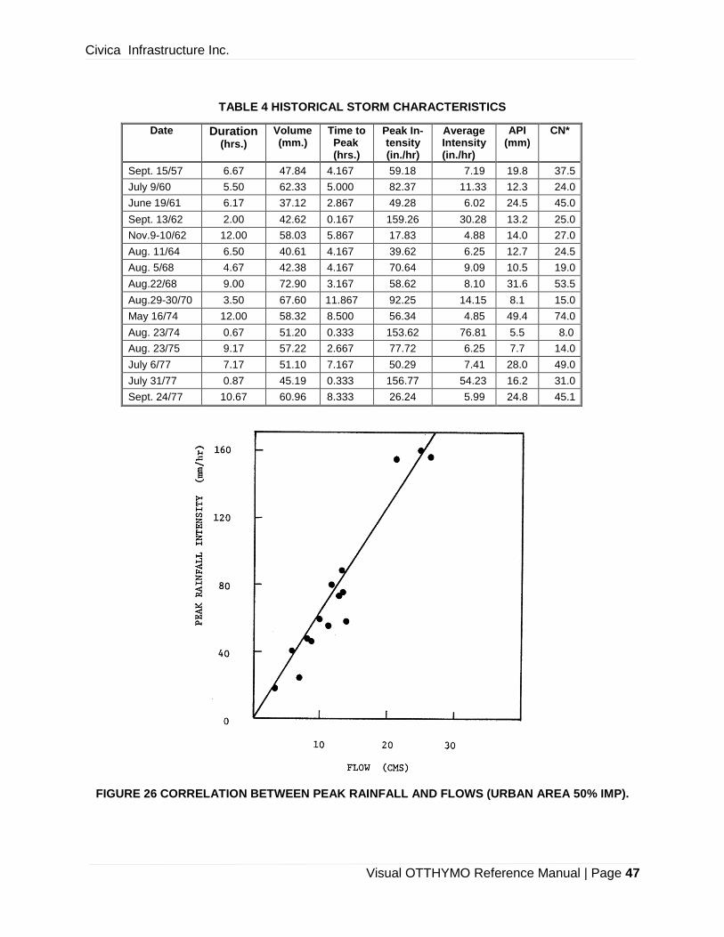
Civica Infrastructure Inc.
Visual OTTHYMO Reference Manual | Page 47
TABLE 4 HISTORICAL STORM CHARACTERISTICS
Date Duration (hrs.)
Volume (mm.)
Time to Peak (hrs.)
Peak In-tensity (in./hr)
Average Intensity (in./hr)
API (mm)
CN*
Sept. 15/57 6.67 47.84 4.167 59.18 7.19 19.8 37.5
July 9/60 5.50 62.33 5.000 82.37 11.33 12.3 24.0
June 19/61 6.17 37.12 2.867 49.28 6.02 24.5 45.0
Sept. 13/62 2.00 42.62 0.167 159.26 30.28 13.2 25.0
Nov.9-10/62 12.00 58.03 5.867 17.83 4.88 14.0 27.0
Aug. 11/64 6.50 40.61 4.167 39.62 6.25 12.7 24.5
Aug. 5/68 4.67 42.38 4.167 70.64 9.09 10.5 19.0
Aug.22/68 9.00 72.90 3.167 58.62 8.10 31.6 53.5
Aug.29-30/70 3.50 67.60 11.867 92.25 14.15 8.1 15.0
May 16/74 12.00 58.32 8.500 56.34 4.85 49.4 74.0
Aug. 23/74 0.67 51.20 0.333 153.62 76.81 5.5 8.0
Aug. 23/75 9.17 57.22 2.667 77.72 6.25 7.7 14.0
July 6/77 7.17 51.10 7.167 50.29 7.41 28.0 49.0
July 31/77 0.87 45.19 0.333 156.77 54.23 16.2 31.0
Sept. 24/77 10.67 60.96 8.333 26.24 5.99 24.8 45.1
FIGURE 26 CORRELATION BETWEEN PEAK RAINFALL AND FLOWS (URBAN AREA 50% IMP).
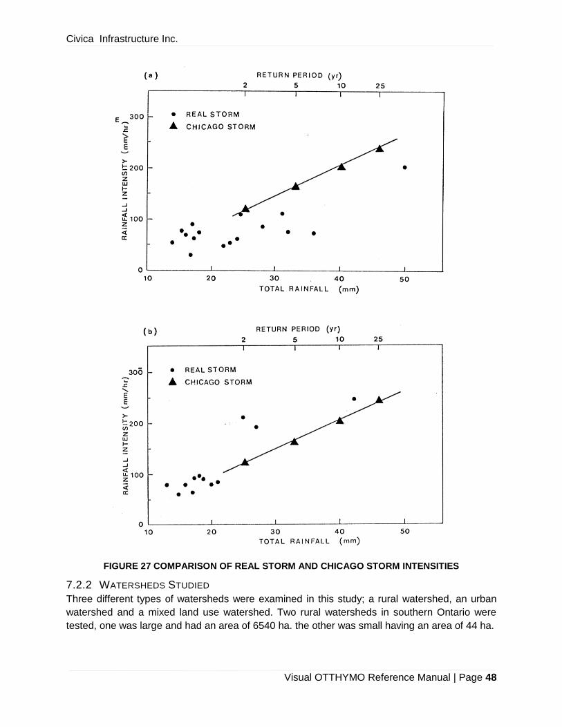
Civica Infrastructure Inc.
Visual OTTHYMO Reference Manual | Page 48
FIGURE 27 COMPARISON OF REAL STORM AND CHICAGO STORM INTENSITIES
7.2.2 WATERSHEDS STUDIED
Three different types of watersheds were examined in this study; a rural watershed, an urban
watershed and a mixed land use watershed. Two rural watersheds in southern Ontario were
tested, one was large and had an area of 6540 ha. the other was small having an area of 44 ha.

Civica Infrastructure Inc.
Visual OTTHYMO Reference Manual | Page 49
Simulation runs were also conducted on three southern Ontario urban watersheds. The catch-
ment characteristics are summarized in Table 5. On two of the catchments the urban area routine
URBHYD of OTTHYMO was used. Impervious conditions of 35% and 50% were used on urban
catchment No.1 to observe the change in difference between the design storm peak flows. On
the third urban catchment the SWMM simulation program was used. A schematic of this catch-
ment is shown in Figure 28.
TABLE 5 URBAN WATERSHED CHARACTERISTICS
Watershed Area (ha.)
Imperviousness (%)
No. 1 294.4 35 & 50
No. 2 290.3 50
No. 3 150.5 30
A mixed land use watershed in Metropolitan Toronto, having a rural area of 1597 ha. and an urban
area of 5536 ha., as also tested. The flows on this watershed were found using the OTTHYMO
model. The total area contained 21 urban subwatersheds and 12 rural subwatersheds. They
ranged in size from 53 ha. to 778 ha. The urban subwatersheds had an imperviousness of 35%.
7.2.3 SIMULATION MODELS AND THEIR CALIBRATION
The two, single event simulation models used to test the design storms were the SWMM and the
OTTHYMO models. The SWMM model was used on urban catchment No.3. The Chicago design
storm with a 10 min. time step, was compared with a series of flows generated from real storms.
The antecedent moisture conditions are accounted for using values for the Horton equation’s
initial infiltration capacity and final infiltration capacity.
The lumped OTTHYMO model was used on the rural, urban and mixed watersheds. The rural
watershed in southern Ontario is used as an example to show how the model was calibrated. The
catchment data was first obtained and used to compute the time to peak Tp and the storage
coefficient K. The initial abstraction Ia was found by examining the rainfall record and the stream
flow record and distinguishing between the rainfall events that produce runoff and those that do
not produce runoff. The relationship between the modified curve number CN* and the antecedent
precipitation index API was found using five storm events for which there were discretized rainfall
measurements as well as stream flow records. Simulations were then conducted and the gener-
ated hydrographs were compared with the measured hydrographs and found to be similar. The
model was therefore properly calibrated.
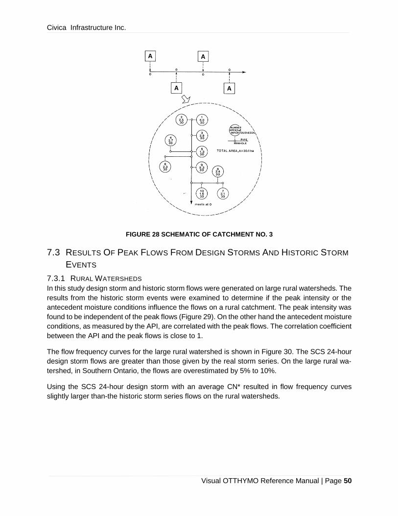
Civica Infrastructure Inc.
Visual OTTHYMO Reference Manual | Page 50
FIGURE 28 SCHEMATIC OF CATCHMENT NO. 3
7.3 RESULTS OF PEAK FLOWS FROM DESIGN STORMS AND HISTORIC STORM
EVENTS
7.3.1 RURAL WATERSHEDS
In this study design storm and historic storm flows were generated on large rural watersheds. The
results from the historic storm events were examined to determine if the peak intensity or the
antecedent moisture conditions influence the flows on a rural catchment. The peak intensity was
found to be independent of the peak flows (Figure 29). On the other hand the antecedent moisture
conditions, as measured by the API, are correlated with the peak flows. The correlation coefficient
between the API and the peak flows is close to 1.
The flow frequency curves for the large rural watershed is shown in Figure 30. The SCS 24-hour
design storm flows are greater than those given by the real storm series. On the large rural wa-
tershed, in Southern Ontario, the flows are overestimated by 5% to 10%.
Using the SCS 24-hour design storm with an average CN* resulted in flow frequency curves
slightly larger than-the historic storm series flows on the rural watersheds.
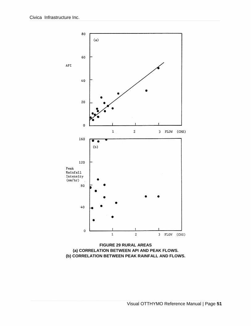
Civica Infrastructure Inc.
Visual OTTHYMO Reference Manual | Page 51
FIGURE 29 RURAL AREAS
(a) CORRELATION BETWEEN API AND PEAK FLOWS.
(b) CORRELATION BETWEEN PEAK RAINFALL AND FLOWS.
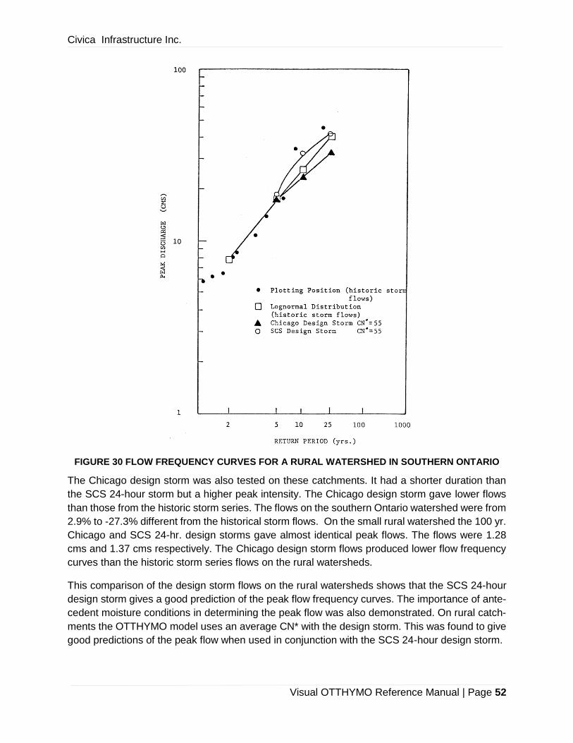
Civica Infrastructure Inc.
Visual OTTHYMO Reference Manual | Page 52
FIGURE 30 FLOW FREQUENCY CURVES FOR A RURAL WATERSHED IN SOUTHERN ONTARIO
The Chicago design storm was also tested on these catchments. It had a shorter duration than
the SCS 24-hour storm but a higher peak intensity. The Chicago design storm gave lower flows
than those from the historic storm series. The flows on the southern Ontario watershed were from
2.9% to -27.3% different from the historical storm flows. On the small rural watershed the 100 yr.
Chicago and SCS 24-hr. design storms gave almost identical peak flows. The flows were 1.28
cms and 1.37 cms respectively. The Chicago design storm flows produced lower flow frequency
curves than the historic storm series flows on the rural watersheds.
This comparison of the design storm flows on the rural watersheds shows that the SCS 24-hour
design storm gives a good prediction of the peak flow frequency curves. The importance of ante-
cedent moisture conditions in determining the peak flow was also demonstrated. On rural catch-
ments the OTTHYMO model uses an average CN* with the design storm. This was found to give
good predictions of the peak flow when used in conjunction with the SCS 24-hour design storm.

Civica Infrastructure Inc.
Visual OTTHYMO Reference Manual | Page 53
7.3.2 URBAN WATERSHEDS
The dependence of the historic storm flows to the peak intensity and antecedent moisture condi-
tions were examined on the urban catchments. The peak intensity was found to be an important
factor in determining the peak flows. The correlation between the peak intensity and peak flows
was close to 1 (Figure 29). Antecedent moisture conditions do not show any correlation with the
peak flows (Figure 31). It was found that runoff from urban catchments was independent of CN*.
The SCS 24-hour design storm flows were compared with the historic storm series flows on urban
watersheds No.1 and No.2. The comparison of the flows is shown on Figures 32 and 33. The
SCS 24-hour design storm underestimated the flow on both of the watersheds. On watershed
No.1 the flow was underestimated by 11% to 22% while on watershed No.2 from 14% to 26%.
On these urban watersheds the SCS 24-hour design storm has underestimated the peak flow.
The Chicago design storm was tested on the three urban watersheds. The flow predictions given
by this storm are slightly below the historical storm series on urban areas No.1 and No.2 (Figures
32 and 33). The flows were underestimated by approximately 6% on watershed No.1 and 4% on
watershed No.2. On urban watershed No.3 the SWMM simulation program was used. The Chi-
cago storm gave results that were similar to the real storm flows (Figure 34). From the tests con-
ducted on these three urban areas the Chicago design storm gave peak flow predictions close to
the flows from the historic storm series.
The effect of changing the catchment imperviousness was examined on urban watershed No.1.
Flows were generated on this catchment using the design storms and the historic storms for im-
pervious conditions of 35% and 50%. The flow frequency curves for the two impervious conditions
are shown in Figure 34. Increasing the catchment imperviousness resulted in the SCS storm
giving lower flows with respect to the real storm series. The relative position of the Chicago storm
flows did not change. The Chicago storm is less sensitive to changes in the catchment impervi-
ousness than the SCS 24-hour storm.
The comparison of the design storms on the urban catchments has shown that the Chicago storm
gives a good prediction of peak flow on urban catchments. Flows in the urban areas were found
to be dependent on peak intensity and independent of antecedent moisture conditions. The sen-
sitivity of peak flows to peak intensities showed the importance of having design storm peak in-
tensities similar to real storm peak intensities.
The Chicago storm that was used obtained the peak intensities by having a 10 minute step size.
Increasing the imperviousness of urban catchment No.1 demonstrated that the Chicago design
storm continued to give a good prediction of the peak flow. For these reasons the Chicago design
storm may be used with single event simulation models on urban watersheds.
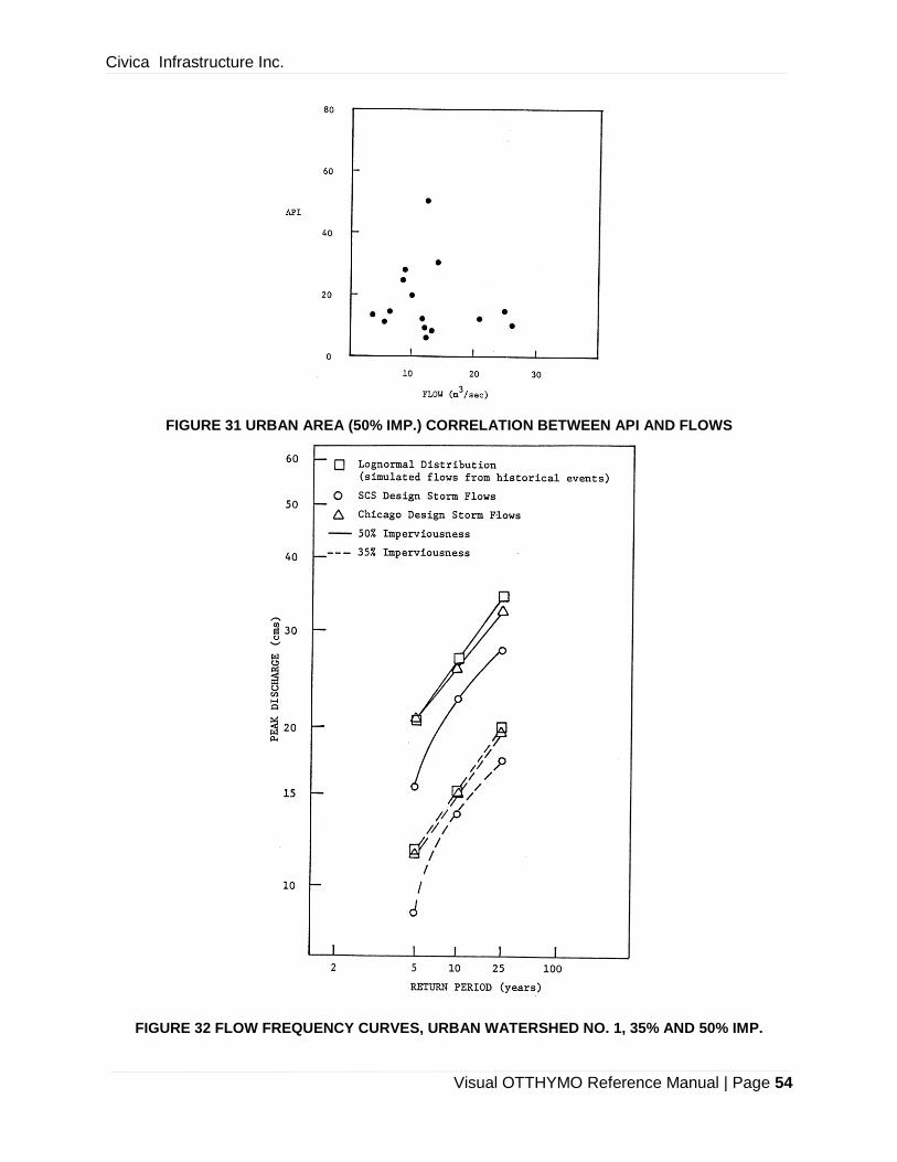
Civica Infrastructure Inc.
Visual OTTHYMO Reference Manual | Page 54
FIGURE 31 URBAN AREA (50% IMP.) CORRELATION BETWEEN API AND FLOWS
FIGURE 32 FLOW FREQUENCY CURVES, URBAN WATERSHED NO. 1, 35% AND 50% IMP.
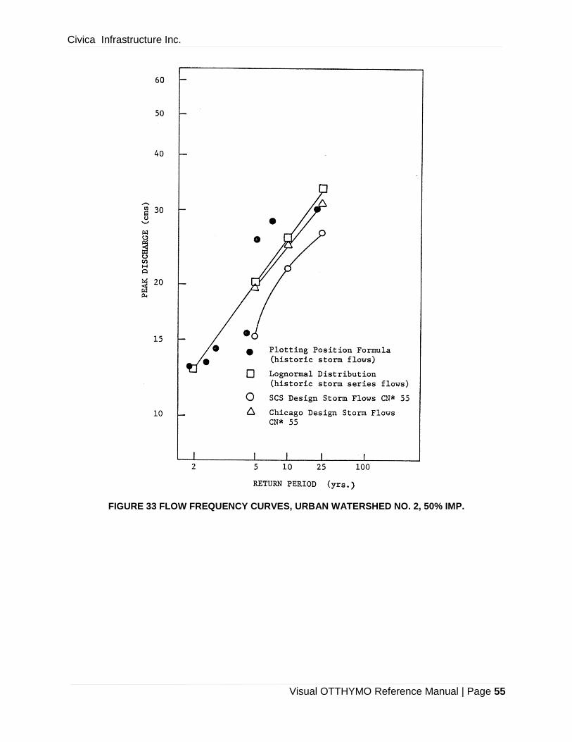
Civica Infrastructure Inc.
Visual OTTHYMO Reference Manual | Page 55
FIGURE 33 FLOW FREQUENCY CURVES, URBAN WATERSHED NO. 2, 50% IMP.
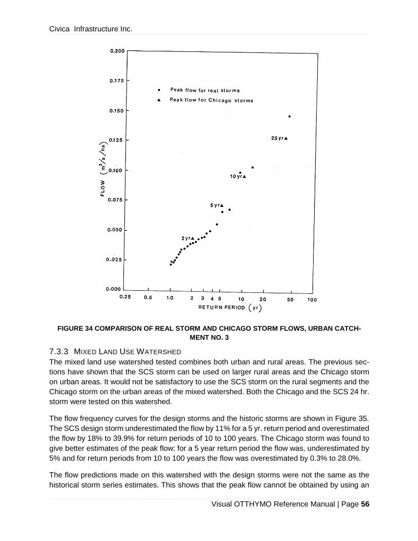
Civica Infrastructure Inc.
Visual OTTHYMO Reference Manual | Page 56
FIGURE 34 COMPARISON OF REAL STORM AND CHICAGO STORM FLOWS, URBAN CATCH-
MENT NO. 3
7.3.3 MIXED LAND USE WATERSHED
The mixed land use watershed tested combines both urban and rural areas. The previous sec-
tions have shown that the SCS storm can be used on larger rural areas and the Chicago storm
on urban areas. It would not be satisfactory to use the SCS storm on the rural segments and the
Chicago storm on the urban areas of the mixed watershed. Both the Chicago and the SCS 24 hr.
storm were tested on this watershed.
The flow frequency curves for the design storms and the historic storms are shown in Figure 35.
The SCS design storm underestimated the flow by 11% for a 5 yr. return period and overestimated
the flow by 18% to 39.9% for return periods of 10 to 100 years. The Chicago storm was found to
give better estimates of the peak flow; for a 5 year return period the flow was, underestimated by
5% and for return periods from 10 to 100 years the flow was overestimated by 0.3% to 28.0%.
The flow predictions made on this watershed with the design storms were not the same as the
historical storm series estimates. This shows that the peak flow cannot be obtained by using an
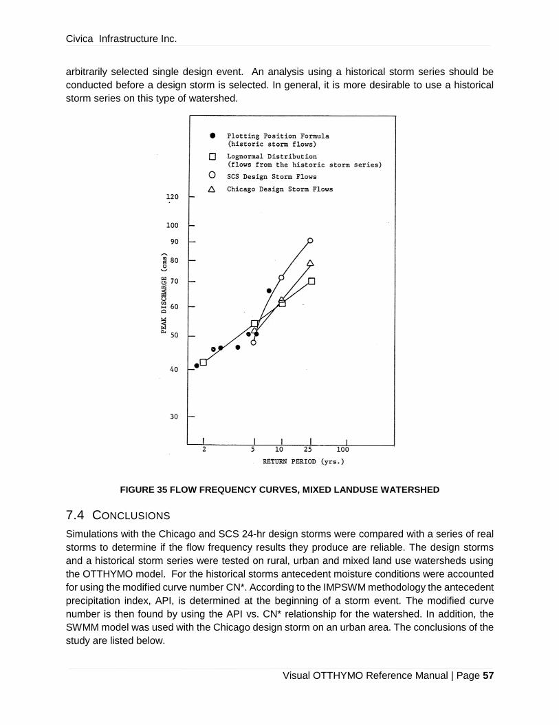
Civica Infrastructure Inc.
Visual OTTHYMO Reference Manual | Page 57
arbitrarily selected single design event. An analysis using a historical storm series should be
conducted before a design storm is selected. In general, it is more desirable to use a historical
storm series on this type of watershed.
FIGURE 35 FLOW FREQUENCY CURVES, MIXED LANDUSE WATERSHED
7.4 CONCLUSIONS
Simulations with the Chicago and SCS 24-hr design storms were compared with a series of real
storms to determine if the flow frequency results they produce are reliable. The design storms
and a historical storm series were tested on rural, urban and mixed land use watersheds using
the OTTHYMO model. For the historical storms antecedent moisture conditions were accounted
for using the modified curve number CN*. According to the IMPSWM methodology the antecedent
precipitation index, API, is determined at the beginning of a storm event. The modified curve
number is then found by using the API vs. CN* relationship for the watershed. In addition, the
SWMM model was used with the Chicago design storm on an urban area. The conclusions of the
study are listed below.

Civica Infrastructure Inc.
Visual OTTHYMO Reference Manual | Page 58
1. In rural areas antecedent moisture conditions were shown to be critical in determining
peak flows.
2. A modified curve number was calibrated which in conjunction with the SCS 24-hr. design
storm gives adequate results on rural watersheds. This "design curve number" is proposed
to be part of the design storm concept.
3. Using the "calibrated design curve number" on large rural watersheds it was found that
Chicago design storms underestimate the flow. The SCS 24-hr design storm gave good
flow predictions on both large and small rural watersheds. For a small rural watershed the
difference between the Chicago and SC-S 24-hr peak flow was found to minimal.
4. For urban areas the SCS 24-hr design storm underestimated the peak flow. The Chicago
storm gave consistent peak flow results. It was also demonstrated that the peak intensity
is an important factor in determining he peak flows in urban areas. For this reason design
storm peak intensities should be selected on the basis of a study of peak intensities of
critical real storm events.
5. On the large mixed land use watershed antecedent moisture conditions must be consid-
ered if the contribution of the rural watershed is important. For flood control purposes in
large mixed areas it is preferable to use a series of real storms. One cannot tell prior to
analysis of the watershed which design storm will produce acceptable results.
6. Results found for the homogeneous watershed indicate that for routine SWM studies de-
sign storms can be used. It is however desirable to compare the two types of design
storms and eventually a critical historic storm.

Civica Infrastructure Inc.
Visual OTTHYMO Reference Manual | Page 59
8 A REVIEW OF DESIGN STORM PROFILES
8.1 INTENSITY DURATION FREQUENCY CURVES
In Canada, the Atmospheric Environment Service (AES) of Environment Canada does the collec-
tion of rainfall records. The rainfall amounts are collected using a tipping bucket rain gauge. The
rain gauge typically records every 0.01 inches of rainfall. The AES standard procedure locates an
Type B Standard Rain Gauge (AES standard) together with the tipping bucket and adjusts the
tipping bucket data so that the daily totals of both gauges agree. In the United States the U.S.
Weather Service collects data which is then stored and analyzed at the National Climate Centre
(NOAA, Environmental Data Service Ashville N.C.). Worldwide meteorological information may
be obtained from the World Meteorological Organization.
The AES analyzes the daily records obtained from the tipping bucket rain gauge. In the case of
strip charts, these are analyzed to determine the maximum rainfall volume occurring in 5, 10, 15,
30, 60, 120, 360, 720, and 1440 minute intervals during each day of a year. The daily record of
maximum volumes is scanned at the end of each year to determine the annual maximum volumes
for each of the time periods. This analysis is conducted for every year of the rainfall record to form
an annual maximum series. Each set of volumes is divided by the appropriate fixed duration to
obtain the annual maximum series for intensities.
The return period of extreme intensities is of special interest to engineers who want to calculate
the return period of the rainfall-induced peak flows. The return period can be determined using a
plotting position formula or by using an extreme-value distribution. For example, the Atmospheric
Environment Service uses the extreme value type 1 distribution. The statistical parameters of
mean, standard deviation and skew are computed for each set of annual maximum intensities.
The intensity of a particular frequency is computed using the statistical parameters and the fre-
quency factor form of the probability distribution (Chow,1954). For each duration, the intensities
for the desired return periods are computed. The points of intensity and duration for known return
periods are plotted. Lines joining all the points having the same return period are drawn to form
an IDF curve. An example of the intensity-duration-frequency (IDF) curves developed by the AES
for the Bloor Street station in Toronto are shown in Figure 36.
Engineers have also found advantageous to fit empirical equations to the statistically developed
IDF curves. Equations 35 and 36 are the general forms of the empirical equations used most
frequently.
𝑖 =𝑎
(𝑡 + 𝑐)𝑏 (35)
𝑖 =𝑎
𝑡𝑏 + 𝑐 (36)
To describe the variation in average intensity with duration for a given frequency, the parameters
a, b and c must be determined. This is done by fitting the either of the two equations to the statis-
tically determined values for i and t. The value of b is estimated, then the following equation can
be solved for the constants c and ln(a).
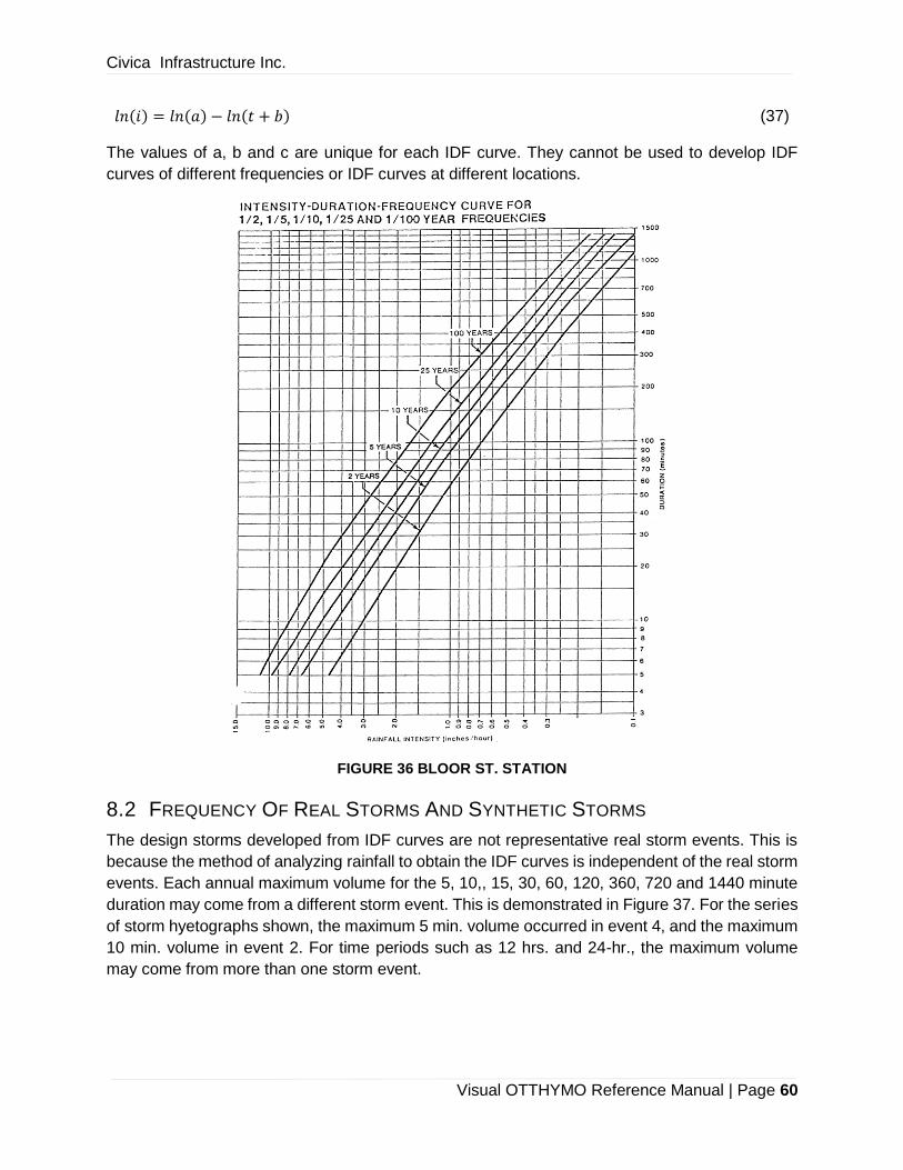
Civica Infrastructure Inc.
Visual OTTHYMO Reference Manual | Page 60
𝑙𝑛(𝑖) = 𝑙𝑛(𝑎) − 𝑙𝑛(𝑡 + 𝑏) (37)
The values of a, b and c are unique for each IDF curve. They cannot be used to develop IDF
curves of different frequencies or IDF curves at different locations.
FIGURE 36 BLOOR ST. STATION
8.2 FREQUENCY OF REAL STORMS AND SYNTHETIC STORMS
The design storms developed from IDF curves are not representative real storm events. This is
because the method of analyzing rainfall to obtain the IDF curves is independent of the real storm
events. Each annual maximum volume for the 5, 10,, 15, 30, 60, 120, 360, 720 and 1440 minute
duration may come from a different storm event. This is demonstrated in Figure 37. For the series
of storm hyetographs shown, the maximum 5 min. volume occurred in event 4, and the maximum
10 min. volume in event 2. For time periods such as 12 hrs. and 24-hr., the maximum volume
may come from more than one storm event.

Civica Infrastructure Inc.
Visual OTTHYMO Reference Manual | Page 61
FIGURE 37 REAL STORM HYETOGRAPHS
In a real storm event, the maximum average intensities for fixed duration within the event have
different frequencies. Real storm events do not have a single frequency. For example, event 4
has a return period of 2 yrs. for the 5 min. duration, a return period of 1 year for the 10 minute
duration, and a 2 year return period for the average intensity of the total event duration. The
frequency of average intensity for different duration in some storms may vary from 1 yr. to 50
years. Design storms on the other hand are developed so that the maximum average intensity for
each fixed duration in the design storm has the same frequency. Since design storm are devel-
oped from IDF curves, they contain the maximum average intensities from different storm events.
Design storms are therefore models of real storms and their validity requires testing.
8.3 UNIFORM DESIGN STORM
The uniform design storm is the oldest and simplest design storm. The storm originates from the
use of the rational method. By selecting a duration and return period, the average maximum in-
tensity is found from an intensity .duration frequency curve. The intensity remains constant for the
duration of the storm.
The uniform design storm contains only a part of the real storm volumes. The volume of the uni-
form design storm is obtained from an IDF curve it is not the volume from a real storm event. The
uniform hyetograph does not show any variation in intensity with time. Real rainfall events have
intensities that are highly variable, this variability affects the peak flow.

Civica Infrastructure Inc.
Visual OTTHYMO Reference Manual | Page 62
8.4 COMPOSITE DESIGN STORM
To develop this design storm, the storm duration is first selected. Average intensities are then
found by reading an IDF curve at selected duration shorter than the storm duration. The selected
duration should be separated by a constant time step. Next, the accumulated storm volume is
computed by multiplying each duration by the average intensity. The incremental rainfall volumes
and intensities are computed and then arbitrarily rearranged to form a storm pattern. If the incre-
mental intensities are not rearranged a front-end hyetograph, following the shape of the IDF curve,
is obtained.
8.5 CHICAGO DESIGN STORM
The Chicago design storm is a design storm distribution widely used by practising drainage engi-
neers. This representation of the temporal distribution of rainfall was proposed by Keifer and Chu
in 1957. They developed a storm pattern which would preserve the maximum volume of water
falling within a specified duration, the average amount of rainfall before the peak intensity and the
relative time of the peak intensity.
To determine the time distribution of rainfall and preserve the previously mentioned characteris-
tics, they adopted the empirical IDF curves. By using IDF curves, they stayed with a procedure
and concepts engineers were familiar with and is simple to obtain and therefore, it has become
widely accepted for use in engineering practice.
8.5.1 DERIVATION OF THE CHICAGO DESIGN STORM
The Chicago design storm is developed from empirical IDF relationships. Keifer and Chu ob-
served that if they had a continuous function representation of the instantaneous intensity and
they integrated this function over a given duration, the rainfall volume occurring in that duration is
obtained. The rainfall volume divided by the duration gives the average intensity. Therefore, mul-
tiplying the average intensity by the storm duration and differentiating with respect to the duration
they obtained expressions for the instantaneous intensity:
𝑖 =𝑎((1 − 𝑐)𝑡 + 𝑏)
(𝑡 + 𝑏)𝑐+1 (38)
𝑖 =𝑎 ((1 − 𝑏)𝑡𝑏 + 𝑐)
(𝑡𝑏 + 𝑐)2
(39)
These equations for the shape of the storm hyetograph are for a storm pattern where the peak is
at the beginning of the storm event. If the peak occurs after the beginning of the storm, the storm
duration t is divided into two time periods, the time before the peak tb and the time after the peak
ta. The ratio of the time to peak to the total storm duration is given by the equation:
𝑟 =𝑡𝑏
𝑡 (40)
The storm duration in terms of the time before the peak and the time after the peak is given by
equations:
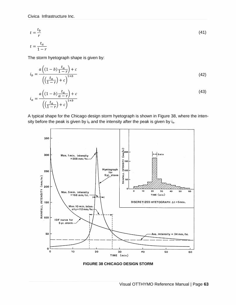
Civica Infrastructure Inc.
Visual OTTHYMO Reference Manual | Page 63
𝑡 =𝑡𝑏
𝑟 (41)
𝑡 =𝑡𝑎
1 − 𝑟
The storm hyetograph shape is given by:
𝑖𝑏 =𝑎 ((1 − 𝑏)
𝑡𝑎1 − 𝑟
) + 𝑐
((𝑡𝑎
1 − 𝑟) + 𝑐)1+𝑏
(42)
𝑖𝑎 =𝑎 ((1 − 𝑏)
𝑡𝑎𝑎 − 𝑟
) + 𝑐
((𝑡𝑎
1 − 𝑟) + 𝑐)1+𝑏
(43)
A typical shape for the Chicago design storm hyetograph is shown in Figure 38, where the inten-
sity before the peak is given by ib and the intensity after the peak is given by ia.
FIGURE 38 CHICAGO DESIGN STORM

Civica Infrastructure Inc.
Visual OTTHYMO Reference Manual | Page 64
8.5.2 PARAMETER ESTIMATION
The procedure for determining the constants for the empirical IDF curve was discussed previously
in the Intesity Duration Frequency Curves section. The only constant that is required for the Chi-
cago design storm is the ratio of the time before the peak to the storm duration, r. Two procedures
may be used to determine the value of r:
1. The ratio of time to peak intensity to the storm duration is computed for a series of events
for various duration. For a given duration, the average time to peak is determined from a
number of rainfall events of that duration. This is done for a set of duration. The mean
value of the time to peak to the storm duration ratio is computed as a weighted average.
The following equation (is an example of how r is computed.
𝑟 =𝑡𝑑1(𝑡�̅�1) + 𝑡𝑑2(𝑡�̅�2) + 𝑡𝑑3(𝑡�̅�2)
𝑡𝑑1 + 𝑡𝑑2 + 𝑡𝑑3 (44)
where, 𝑡𝑑1, 𝑡𝑑2, 𝑡𝑑3 are the durations of the different rainfall occurrences, 𝑡�̅�1, 𝑡�̅�2, 𝑡�̅�3 are
the average time to. peak for the different rainfall occurrences and r is the ratio of time to
peak to total storm duration.
2. The ratio can be computed by analyzing local storm distributions to determine the rainfall
depth before the peak intensity. The design storm duration is then chosen. The rainfall
depth prior to the peak is determined for durations less than the design storm. A weighted
average for r is determined based on the ratio of the antecedent rainfall depth to the total
rainfall depth. This is done by using:
𝑑𝑎 = 𝑟(𝑡𝑑𝐼𝑡𝑑 − 𝑡𝐼𝑡) (45)
where:
𝑑𝑎= depth of antecedent rainfall,
𝑡𝑑 = design storm duration,
𝑡 = rainfall duration,
𝐼𝑡𝑑= maximum average intensity for the total duration,
𝐼𝑡 = maximum average intensity for duration t.
Specific applications of each procedure have been documented. For example, McPherson (1958)
has criticized the second procedure while both have been demonstrated by Bandyopadhyay
(1972). The later obtained a value 0.416 for the first procedure and an r value of 0.37 for the
second. Table 6 presents a list of r values obtained by different researchers.

Civica Infrastructure Inc.
Visual OTTHYMO Reference Manual | Page 65
TABLE 6 VALUES OF R FOR THE CHICAGO DESIGN STORM
Location R Source
Baltimore 0.399 McPherson, 1958
Chicago 0.375 Keifer and Chu, 1957
Cincinnati 0.325 Preul et al., 1973
Ontario 0.488 Marsalek, 1978
Philadelphia 0.414 McPherson, 1958
8.5.3 DETERMINATION OF THE CHICAGO DESIGN STORM HYETOGRAPH
The steps to produce a Chicago design storm Hyetograph are:
1. Select a design storm duration.
2. Select a time step . The time step size should not be less than the minimum duration that
was used when determining the IDF curves. For the Canadian IDF curves, step size
should be at least 5 minutes. It is recommended that the step size should be about 10
minutes.
If the parameters a, b, c and r for the Chicago design storm are not known they should be deter-
mined.
The instantaneous rainfall intensities at the different time intervals from the peak intensity are
computed.
8.6 SCS 24-HOUR DESIGN STORM
The U.S. Soil Conservation Service (SCS) has developed the ‘Type 1 and 2’ design storm. These
have and are used both, in the U.S.A. and Canada. The SCS determined the mass curve for
percent of accumulated rainfall depth over a duration of 24-hr. To obtain the mass curve, rainfall
was analyzed across the U.S.. SCS characterized the rainfall using the 2 types of storm patterns:
The Type 1 rainfall distribution is applicable to Hawaii, Alaska, the Coastal Sierra Nevada, the
Cascade Mountains in California, Oregon and Washington. The type 2 rainfall distribution applies
to the remainder of the United States, Puerto Rico and the Virgin Islands. Figure 39 illustrates the
SCS 24-hour rainfall distribution. In Canada, the type 2 curve applies in most areas, however,
there are some regions in British Columbia where the type 1 curve is used.
To create a SCS design storm, a duration and return period is first selected. The corresponding
volume is then distributed over the steepest portion of the SCS-24 hour curve. The incremental
rainfall volumes and intensities are then obtained based on the volume distribution over the se-
lected duration.
It’s worth noting that the Composite Design Storm can be rearranged to give a storm pattern very
similar to the SCS design storm. This occurs because the SCS type 1 and type 2 curves have
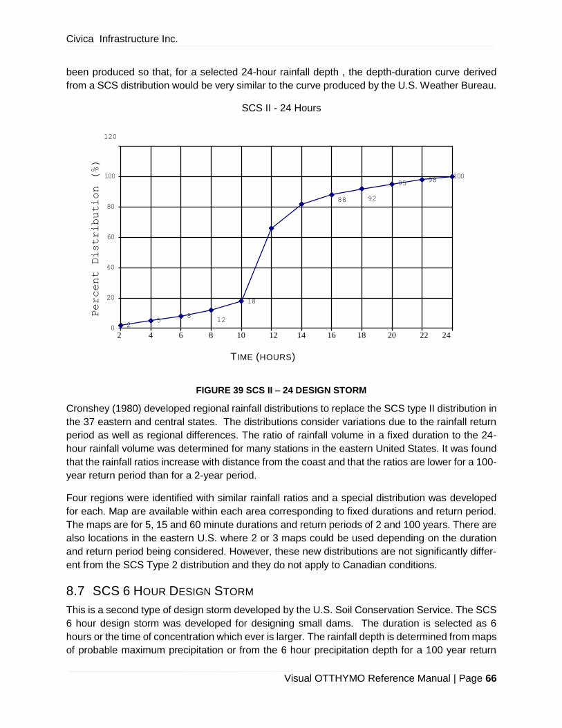
Civica Infrastructure Inc.
Visual OTTHYMO Reference Manual | Page 66
88
92
95 98
2 5
8
12
18
100 100
80
60
40
20
0
been produced so that, for a selected 24-hour rainfall depth , the depth-duration curve derived
from a SCS distribution would be very similar to the curve produced by the U.S. Weather Bureau.
SCS II - 24 Hours
120
2 4 6 8 10 12 14 16 18 20 22 24
TIME (HOURS)
FIGURE 39 SCS II – 24 DESIGN STORM
Cronshey (1980) developed regional rainfall distributions to replace the SCS type II distribution in
the 37 eastern and central states. The distributions consider variations due to the rainfall return
period as well as regional differences. The ratio of rainfall volume in a fixed duration to the 24-
hour rainfall volume was determined for many stations in the eastern United States. It was found
that the rainfall ratios increase with distance from the coast and that the ratios are lower for a 100-
year return period than for a 2-year period.
Four regions were identified with similar rainfall ratios and a special distribution was developed
for each. Map are available within each area corresponding to fixed durations and return period.
The maps are for 5, 15 and 60 minute durations and return periods of 2 and 100 years. There are
also locations in the eastern U.S. where 2 or 3 maps could be used depending on the duration
and return period being considered. However, these new distributions are not significantly differ-
ent from the SCS Type 2 distribution and they do not apply to Canadian conditions.
8.7 SCS 6 HOUR DESIGN STORM
This is a second type of design storm developed by the U.S. Soil Conservation Service. The SCS
6 hour design storm was developed for designing small dams. The duration is selected as 6
hours or the time of concentration which ever is larger. The rainfall depth is determined from maps
of probable maximum precipitation or from the 6 hour precipitation depth for a 100 year return
Percent Distribution (%)

Civica Infrastructure Inc.
Visual OTTHYMO Reference Manual | Page 67
period. The hyetograph profile is determined using a 6 hour design storm distribution, an example
is shown in Figure 40.
This storm was developed for use in conjunction-with the SCS method of runoff computation. With
the SCS method the rainfall depth and duration must be known. The watershed soil type and
antecedent moisture conditions are also important. These catchment characteristics are reflected
in the SCS curve number. The-amount of direct runoff is computed using the total precipitation
and the curve number. The hyetograph shape is not important in determining the direct runoff with
the SCS method. It is important, though, when the runoff is computed using a single event simu-
lation model.
The rainfall depth for the SCS 6 hour design storm has not been determined using Canadian
meteorological data. It therefore should not be used on Canadian catchments unless local data
is used.
The return period is much larger than is typically used in urban drainage design. The design storm
was developed for rural conditions and should therefore not be used in urban areas.
FIGURE 40 6-HOUR DESIGN STORM DISTRIBUTION
8.8 ILLINOIS STATE WATER SURVEY DESIGN STORM
The Illinois State Water Survey (ISWS) design storm is based on research conducted by Huff
(1967). Huff examined storm events in central Illinois having durations between 3 hours to 48
hours. He divided the storms into 4 groups depending on the time period in which the majority of
the rain occurred. The storms with the most of the rain occurring in the first quarter of the event
duration are termed first quartile. All of the storm events that examined were placed in one of the
four quartile groups. The rainfall mass curves in each quartile group were determined for various
probability levels (Figure 41). It was found that short duration storm events dominate the first and
second quartile. For this reason, the median distribution in the first quartile is commonly used for

Civica Infrastructure Inc.
Visual OTTHYMO Reference Manual | Page 68
design. Terstriep and Stall (1974) recommended that the first quartile storm with the 50% proba-
bility level be used as the design storm with the Illinois runoff model.
The ISWS design storm is determined by selecting a design storm duration. The maximum depth
for the duration and the given frequency are derived from local data or from an IDF curve. The
rainfall depth is then distributed according to the Huff quartile median distribution.
The ISWS design storm is derived in a similar way to the SCS design storm. When it is used in
Illinois it has the advantage of being developed from an analysis of local data. An analysis of
rainfall similar to Huff's analysis is required if the rainfall structure is to be known for a region other
than Illinois.
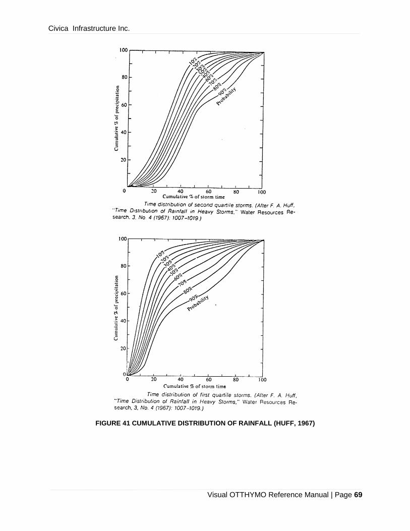
Civica Infrastructure Inc.
Visual OTTHYMO Reference Manual | Page 69
FIGURE 41 CUMULATIVE DISTRIBUTION OF RAINFALL (HUFF, 1967)

Civica Infrastructure Inc.
Visual OTTHYMO Reference Manual | Page 70
8.9 ATMOSPHERIC ENVIRONMENT SERVICE DESIGN STORM
The Canadian Atmospheric Environment Service (AES) examined the temporal variation of rain-
fall using almost 2000 extreme events in Canada. Hogg (1980) conducted the analysis of the time
distribution of rainfall in short duration events. Rainfall duration of 1 and 12 hours were selected
for the analysis and to develop Time-Probability curves. The events were chosen to have samples
from both thunderstorms and large-scale cyclonic origin. The selected events did not have to be
individual storm entities, they could also be part of a larger storm sequence. Fixed rainfall dura-
tions were selected so that the same definition would be used to identify rainfall that is used in
obtaining depth-duration- frequency curves.
In analyzing the rainfall, the one hour events were divided into twelve 5 min. increments and the
12 hour events into 1 hour increments. Rainfall for each event was expressed as a cumulative
percentage of, total event rainfall for the twelve equal increments through the storm. All the events
for a particular duration were analyzed and the cumulative rainfall distributions for different prob-
ability levels were computed (Figure 42).
The temporal distribution patterns were found to vary in the different regions of Canada. The
temporal distributions for the coastal regions were quite different from the distributions for the
continental regions. A comparison was made between Huffs 50% distribution for the second and
third quartile storms and those Hogg developed for southern Ontario. The second quartile distri-
bution was up to 25% different in the cumulative rainfall. The third quartile distribution does not
resemble any of the distributions Hogg computed.
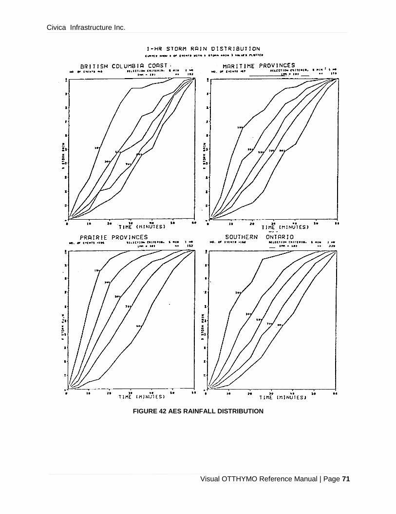
Civica Infrastructure Inc.
Visual OTTHYMO Reference Manual | Page 71
FIGURE 42 AES RAINFALL DISTRIBUTION

Civica Infrastructure Inc.
Visual OTTHYMO Reference Manual | Page 72
8.10 FLOOD STUDIES REPORT DESIGN STORM
The Flood Studies Report (FSR) design storm was developed in the United Kingdom. Rainstorm
profiles of historical events were examined, and the cumulative percentage of rainfall for different
probabilities of storm peakness was developed. The peakness of a storm was defined as the ratio
of maximum to mean intensity. A study of summer and winter storm profiles showed that summer
storms were more peaked than winter storms. The curves of storm peakedness were published
by the National Environment Research Council (NERC,vol.2,1975).
The FSR design storm duration is selected so that the largest peak flow calculated at each point
in the system is taken as the design discharge. The developers of the FSR design storm found
that the peak discharge is not very sensitive to the storm duration, a doubling of duration caused
a change of less than 10% peak discharge. Therefore, a fairly coarse series of rainfall duration
may be used; values of 15, 30, 60, and 120 minutes are recommended. The return period is
selected to be the same as that of the required discharge. This is usually established by the local
government agency.
The rainfall depth is determined using a procedure developed for all of the U.K. Using maps and
a formula, the depth for a particular return period is computed. The depth can also be computed
from a depth-duration-frequency curve.
The antecedent moisture conditions were examined and incorporated into the model developed
by the FSR. The antecedent conditions are expressed by the Urban Catchment Wetness Index
(UCWI). Runoff simulations were conducted on a catchment using a variety of UCWI's for return
periods between 1 and 10 years. An optimum UCWI was found for the catchment that resulted in
good predictions of the peak flow. Similar studies were conducted on other catchments in the U.K.
An analysis of the optimum UCWI’s and rainfall data for the catchments led to a relationship
between the UCWI and the Standard Average Annual Rainfall (SAAR). This relationship can be
used to determine the UCWI for any location in the U.K.
The FSR design storm recommended for use in the U.K. has the following properties:
1. The storm duration should be that which gives the maximum discharge.
2. The return period of rainfall should equal that of the required discharge.
3. The storm profile should be the 50% summer profile.
4. The UCWI varies as the average annual rainfall and should be determined from the Figure
shown below.
Some things to consider before applying this type of storm: A) the FSR design storm peak inten-
sity always occurs at the centre of the storm. B) A local analysis of historic events is not conducted
to determine the time-to-peak. C) The FSR design storm was developed for use in the U.K. only.
A similar analysis would have to be conducted if it was to be used outside the U.K.
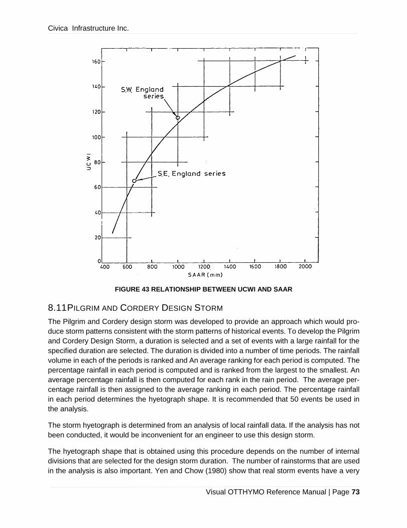
Civica Infrastructure Inc.
Visual OTTHYMO Reference Manual | Page 73
FIGURE 43 RELATIONSHIP BETWEEN UCWI AND SAAR
8.11 PILGRIM AND CORDERY DESIGN STORM
The Pilgrim and Cordery design storm was developed to provide an approach which would pro-
duce storm patterns consistent with the storm patterns of historical events. To develop the Pilgrim
and Cordery Design Storm, a duration is selected and a set of events with a large rainfall for the
specified duration are selected. The duration is divided into a number of time periods. The rainfall
volume in each of the periods is ranked and An average ranking for each period is computed. The
percentage rainfall in each period is computed and is ranked from the largest to the smallest. An
average percentage rainfall is then computed for each rank in the rain period. The average per-
centage rainfall is then assigned to the average ranking in each period. The percentage rainfall
in each period determines the hyetograph shape. It is recommended that 50 events be used in
the analysis.
The storm hyetograph is determined from an analysis of local rainfall data. If the analysis has not
been conducted, it would be inconvenient for an engineer to use this design storm.
The hyetograph shape that is obtained using this procedure depends on the number of internal
divisions that are selected for the design storm duration. The number of rainstorms that are used
in the analysis is also important. Yen and Chow (1980) show that real storm events have a very

Civica Infrastructure Inc.
Visual OTTHYMO Reference Manual | Page 74
uneven temporal distribution of rainfall. For this reason the value of the average ranking of inter-
vals tend to a single number when a large number of rainstorms are used.
8.12 YEN AND CHOW DESIGN STORM
All of the previously discussed design storms were developed from rainfall frequency- duration
relationships or from observations of rain gauge records, they did not use a statistical procedure
to analyze the historical rainfall record. Yen and Chow (1980) use the method of moments to
statistically determine the geometry of hyetograph. Using a triangular hyetograph representation,
only the first moment is required to determine the location of the hyetograph peak.
Rainstorms are analyzed to determine the average depth per time interval
𝑑𝑎𝑣𝑔 =1
𝑛∑ 𝑑𝑗
𝑛
𝑗=1
=𝐷
𝑛 (46)
and the first moment arm of the hyetograph
𝑡𝑎𝑣𝑔 =∆𝑡 ∙ (∑ (𝑗 − 0.5)𝑑𝑗
𝑛𝑗=1 )
𝐷 (47)
where:
𝑛 = number of intervals in the storm,
𝑑𝑗 = rainfall depth in interval j,
𝐷 = total storm depth,
𝑑𝑎𝑣𝑔 = average storm depth,
𝑡 = time step of each interval,
𝑡𝑎𝑣𝑔 = average storm duration.
To describe the hyetograph in more general terms, the hyetograph is non-dimensionalized using
D, the storm depth, and td, the storm duration. The non-dimensionalized form of these two equa-
tions can be expressed in the following two forms:
𝑑𝑎𝑣𝑔0 =
1
𝑛 (48)
𝑡𝑎𝑣𝑔0 =
𝑡̅
𝑡𝑑
(49)
where:
𝑑𝑎𝑣𝑔0 = non-dimensional average storm depth,
𝑡𝑎𝑣𝑔0 =non-dimensional average storm duration.

Civica Infrastructure Inc.
Visual OTTHYMO Reference Manual | Page 75
The hyetograph is described with geometric variables a, b and h. In a non- dimensionalized form,
the variables are expressed by:
𝑎0 = 3𝑡0 (50a)
𝑏0 = 2 − 3𝑡0̅ (50b)
ℎ0 = 2 (50c)
The historical rainfall record is then analyzed to determine values for a, b, h for 6 particular locality.
Yen and Chow have only done this for a rainfall record from Illinois and from Boston. Once the
design storm non-dimensionalized variables are determined, the design storm can be developed.
After selecting the duration and return period, the rainfall depth is found from an IDF curve. Using
the non-dimensionalized variables for the area the design storm is constructed.
The Yen and Chow design storm requires a rainfall data analysis before it can be used in a par-
ticular locality. The non-dimensionalized variable a, can only be found by analyzing a local rainfall
record. It should, not be transported from one locality to another.
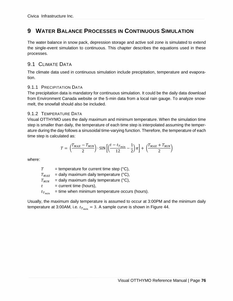
Civica Infrastructure Inc.
Visual OTTHYMO Reference Manual | Page 76
9 WATER BALANCE PROCESSES IN CONTINUOUS SIMULATION
The water balance in snow pack, depression storage and active soil zone is simulated to extend
the single-event simulation to continuous. This chapter describes the equations used in these
processes.
9.1 CLIMATE DATA
The climate data used in continuous simulation include precipitation, temperature and evapora-
tion.
9.1.1 PRECIPITATION DATA
The precipitation data is mandatory for continuous simulation. It could be the daily data download
from Environment Canada website or the 5-min data from a local rain gauge. To analyze snow-
melt, the snowfall should also be included.
9.1.2 TEMPERATURE DATA
Visual OTTHYMO uses the daily maximum and minimum temperature. When the simulation time
step is smaller than daily, the temperature of each time step is interpolated assuming the temper-
ature during the day follows a sinusoidal time-varying function. Therefore, the temperature of each
time step is calculated as:
𝑇 = (𝑇𝑀𝐴𝑋 − 𝑇𝑀𝐼𝑁
2) ∙ SIN [(
𝑡 − 𝑡𝑇𝑚𝑖𝑛
12−
1
2) 𝜋] + (
𝑇𝑀𝐴𝑋 + 𝑇𝑀𝐼𝑁
2)
where:
𝑇 = temperature for current time step (°C),
𝑇𝑀𝐴𝑋 = daily maximum daily temperature (°C),
𝑇𝑀𝐼𝑁 = daily maximum daily temperature (°C),
𝑡 = current time (hours),
𝑡𝑇𝑚𝑖𝑛 = time when minimum temperature occurs (hours).
Usually, the maximum daily temperature is assumed to occur at 3:00PM and the minimum daily
temperature at 3:00AM, i.e. 𝑡𝑇𝑚𝑖𝑛= 3. A sample curve is shown in Figure 44.
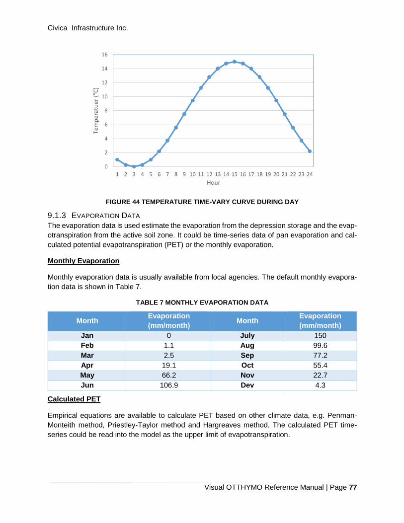
Civica Infrastructure Inc.
Visual OTTHYMO Reference Manual | Page 77
FIGURE 44 TEMPERATURE TIME-VARY CURVE DURING DAY
9.1.3 EVAPORATION DATA
The evaporation data is used estimate the evaporation from the depression storage and the evap-
otranspiration from the active soil zone. It could be time-series data of pan evaporation and cal-
culated potential evapotranspiration (PET) or the monthly evaporation.
Monthly Evaporation
Monthly evaporation data is usually available from local agencies. The default monthly evapora-
tion data is shown in Table 7.
TABLE 7 MONTHLY EVAPORATION DATA
Month Evaporation
(mm/month) Month
Evaporation
(mm/month)
Jan 0 July 150
Feb 1.1 Aug 99.6
Mar 2.5 Sep 77.2
Apr 19.1 Oct 55.4
May 66.2 Nov 22.7
Jun 106.9 Dev 4.3
Calculated PET
Empirical equations are available to calculate PET based on other climate data, e.g. Penman-
Monteith method, Priestley-Taylor method and Hargreaves method. The calculated PET time-
series could be read into the model as the upper limit of evapotranspiration.
0
2
4
6
8
10
12
14
16
1 2 3 4 5 6 7 8 9 10 11 12 13 14 15 16 17 18 19 20 21 22 23 24
Tem
per
atu
er (
°C)
Hour
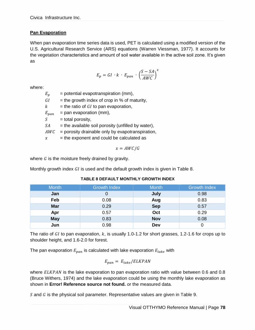
Civica Infrastructure Inc.
Visual OTTHYMO Reference Manual | Page 78
Pan Evaporation
When pan evaporation time series data is used, PET is calculated using a modified version of the
U.S. Agricultural Research Service (ARS) equations (Warren Viessman, 1977). It accounts for
the vegetation characteristics and amount of soil water available in the active soil zone. It’s given
as
𝐸𝑝 = 𝐺𝐼 ∙ 𝑘 ∙ 𝐸𝑝𝑎𝑛 ∙ (𝑆 − 𝑆𝐴
𝐴𝑊𝐶)
𝑥
where:
𝐸𝑝 = potential evapotranspiration (mm),
𝐺𝐼 = the growth index of crop in % of maturity,
𝑘 = the ratio of 𝐺𝐼 to pan evaporation,
𝐸𝑝𝑎𝑛 = pan evaporation (mm),
𝑆 = total porosity,
𝑆𝐴 = the available soil porosity (unfilled by water),
𝐴𝑊𝐶 = porosity drainable only by evapotranspiration,
𝑥 = the exponent and could be calculated as
𝑥 = 𝐴𝑊𝐶/𝐺
where 𝐺 is the moisture freely drained by gravity.
Monthly growth index 𝐺𝐼 is used and the default growth index is given in Table 8.
TABLE 8 DEFAULT MONTHLY GROWTH INDEX
Month Growth Index Month Growth Index
Jan 0 July 0.98
Feb 0.08 Aug 0.83
Mar 0.29 Sep 0.57
Apr 0.57 Oct 0.29
May 0.83 Nov 0.08
Jun 0.98 Dev 0
The ratio of 𝐺𝐼 to pan evaporation, 𝑘, is usually 1.0-1.2 for short grasses, 1.2-1.6 for crops up to
shoulder height, and 1.6-2.0 for forest.
The pan evaporation 𝐸𝑝𝑎𝑛 is calculated with lake evaporation 𝐸𝑙𝑎𝑘𝑒 with
𝐸𝑝𝑎𝑛 = 𝐸𝑙𝑎𝑘𝑒/𝐸𝐿𝐾𝑃𝐴𝑁
where 𝐸𝐿𝐾𝑃𝐴𝑁 is the lake evaporation to pan evaporation ratio with value between 0.6 and 0.8
(Bruce Withers, 1974) and the lake evaporation could be using the monthly lake evaporation as
shown in Error! Reference source not found. or the measured data.
𝑆 and 𝐺 is the physical soil parameter. Representative values are given in Table 9.
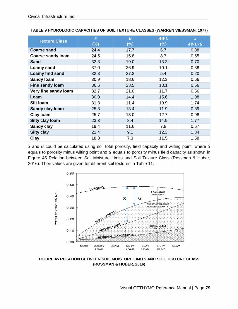
Civica Infrastructure Inc.
Visual OTTHYMO Reference Manual | Page 79
TABLE 9 HYDROLOGIC CAPACITIES OF SOIL TEXTURE CLASSES (WARREN VIESSMAN, 1977)
Texture Class 𝑺
(%)
𝑮
(%)
𝑨𝑾𝑪
(%)
𝒙
𝑨𝑾𝑪/𝑮
Coarse sand 24.4 17.7 6.7 0.38
Coarse sandy loam 24.5 15.8 8.7 0.55
Sand 32.3 19.0 13.3 0.70
Loamy sand 37.0 26.9 10.1 0.38
Loamy find sand 32.3 27.2 5.4 0.20
Sandy loam 30.9 18.6 12.3 0.66
Fine sandy loam 36.6 23.5 13.1 0.56
Very fine sandy loam 32.7 21.0 11.7 0.56
Loam 30.0 14.4 15.6 1.08
Silt loam 31.3 11.4 19.9 1.74
Sandy clay loam 25.3 13.4 11.9 0.89
Clay loam 25.7 13.0 12.7 0.98
Silty clay loam 23.3 8.4 14.9 1.77
Sandy clay 19.4 11.6 7.8 0.67
Silty clay 21.4 9.1 12.3 1.34
Clay 18.8 7.3 11.5 1.58
𝑆 and 𝐺 could be calculated using soil total porosity, field capacity and wilting point, where 𝑆
equals to porosity minus wilting point and 𝐺 equals to porosity minus field capacity as shown in
Figure 45 Relation between Soil Moisture Limits and Soil Texture Class (Rossman & Huber,
2016). Their values are given for different soil textures in Table 11.
FIGURE 45 RELATION BETWEEN SOIL MOISTURE LIMITS AND SOIL TEXTURE CLASS
(ROSSMAN & HUBER, 2016)
S G
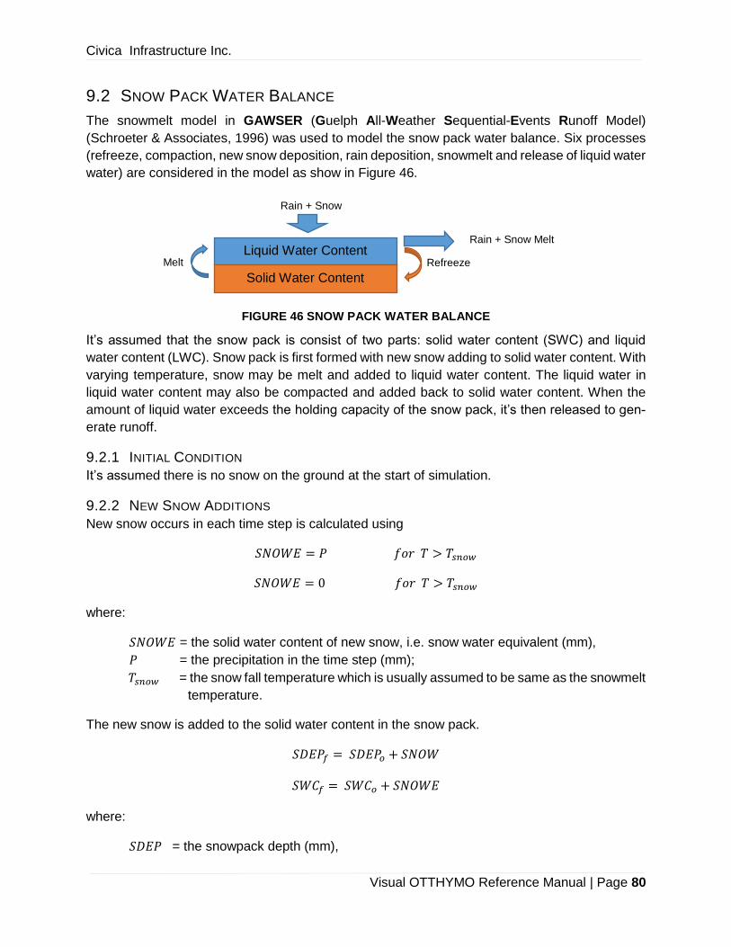
Civica Infrastructure Inc.
Visual OTTHYMO Reference Manual | Page 80
9.2 SNOW PACK WATER BALANCE
The snowmelt model in GAWSER (Guelph All-Weather Sequential-Events Runoff Model)
(Schroeter & Associates, 1996) was used to model the snow pack water balance. Six processes
(refreeze, compaction, new snow deposition, rain deposition, snowmelt and release of liquid water
water) are considered in the model as show in Figure 46.
FIGURE 46 SNOW PACK WATER BALANCE
It’s assumed that the snow pack is consist of two parts: solid water content (SWC) and liquid
water content (LWC). Snow pack is first formed with new snow adding to solid water content. With
varying temperature, snow may be melt and added to liquid water content. The liquid water in
liquid water content may also be compacted and added back to solid water content. When the
amount of liquid water exceeds the holding capacity of the snow pack, it’s then released to gen-
erate runoff.
9.2.1 INITIAL CONDITION
It’s assumed there is no snow on the ground at the start of simulation.
9.2.2 NEW SNOW ADDITIONS
New snow occurs in each time step is calculated using
𝑆𝑁𝑂𝑊𝐸 = 𝑃 𝑓𝑜𝑟 𝑇 > 𝑇𝑠𝑛𝑜𝑤
𝑆𝑁𝑂𝑊𝐸 = 0 𝑓𝑜𝑟 𝑇 > 𝑇𝑠𝑛𝑜𝑤
where:
𝑆𝑁𝑂𝑊𝐸 = the solid water content of new snow, i.e. snow water equivalent (mm),
𝑃 = the precipitation in the time step (mm);
𝑇𝑠𝑛𝑜𝑤 = the snow fall temperature which is usually assumed to be same as the snowmelt
temperature.
The new snow is added to the solid water content in the snow pack.
𝑆𝐷𝐸𝑃𝑓 = 𝑆𝐷𝐸𝑃𝑜 + 𝑆𝑁𝑂𝑊
𝑆𝑊𝐶𝑓 = 𝑆𝑊𝐶𝑜 + 𝑆𝑁𝑂𝑊𝐸
where:
𝑆𝐷𝐸𝑃 = the snowpack depth (mm),
Rain + Snow Melt
Refreeze
Rain + Snow
Melt Liquid Water Content
Solid Water Content
Civica Infrastructure Inc.
Visual OTTHYMO Reference Manual | Page 81
𝑆𝑊𝐶 = the solid (ice) water content (mm), the subscripts 𝑜 and 𝑓 denote the initial and
final values of certain quantities (e.g. 𝑆𝑊𝐶) at the time of the calculation,
𝑆𝑁𝑂𝑊 = the depth of new snowfall calculated using
𝑆𝑁𝑂𝑊 = 𝑆𝑁𝑂𝑊𝐸/𝑁𝐸𝑊𝐷𝐸𝑁
where 𝑁𝐸𝑊𝐷𝐸𝑁 is the relative density of new snow (vol/vol) with default value of 0.1 and range
from 0.02 to 0.15.
As a result of any new snowfall, the relative dry density of the pack, 𝑅𝐻𝑂 (vol/vol) is recalculated
using
𝑅𝐻𝑂 = 𝑆𝑊𝐶/𝑆𝐷𝐸𝑃
And the porosity, 𝑃𝑂𝑅 (vol/vol) is computed from
𝑃𝑂𝑅 = 1 − 𝑅𝐻𝑂/𝑅𝐻𝑂𝐼𝐶𝐸
where 𝑅𝐻𝑂𝐼𝐶𝐸 is the relative density of ice, usually taken as 0.92.
9.2.3 SNOWMELT
A temperature index method is employed to find the potential amount of snowmelt, 𝑀𝐸𝐿𝑇𝑃 (mm)
during the time step, where 𝑀𝐸𝐿𝑇𝑃 is the liquid water depth created by ice crystal melt.
𝑀𝐸𝐿𝑇𝑃 =𝐾𝑀
24∗ 𝐷𝐻 𝑓𝑜𝑟 𝑇 > 𝑇𝐵𝐴𝑆
𝑀𝐸𝐿𝑇𝑃 = 0 𝑓𝑜𝑟 𝑇 ≤ 𝑇𝐵𝐴𝑆
Where:
𝐾𝑀 = the melt factor (mm/d-°C),
𝐷𝐻 = degree hour (hr-°C),
𝑇𝐵𝐴𝑆 = snowmelt temperature (°C).
The melt factor 𝐾𝑀 varies by season and it’s described by
𝐾𝑀 = (𝐾𝑀𝑀𝐴𝑋 − 𝐾𝑀𝑀𝐼𝑁
2) ∙ SIN [(
𝑀𝑜𝑛 − 𝑀𝑜𝑛𝐾𝑀𝑚𝑖𝑛
6−
1
2) 𝜋] + (
𝐾𝑀𝑀𝐴𝑋 + 𝐾𝑀𝑀𝐼𝑁
2)
Where:
𝐾𝑀𝑀𝐴𝑋 = the maximum melt factor which usually occurs in June (mm/d-°C),
𝐾𝑀𝑀𝐼𝑁 = the minimum melt factor which usually occurs in December (mm/d-°C),
𝑀𝑜𝑛 = the month plus the ratio of current day in the month,
𝑀𝑜𝑛𝐾𝑀𝑚𝑖𝑛 = the month when the minimum melt factor occur.
With 𝐾𝑀𝑀𝐴𝑋 = 6.2, 𝐾𝑀𝑀𝐼𝑁 = 2.9 and 𝑀𝑜𝑛𝐾𝑀𝑚𝑖𝑛= 12, the variation is shown in Figure 47. The
snow melt temperature 𝑇𝐵𝐴𝑆 is also assumed to follow the similar variation.
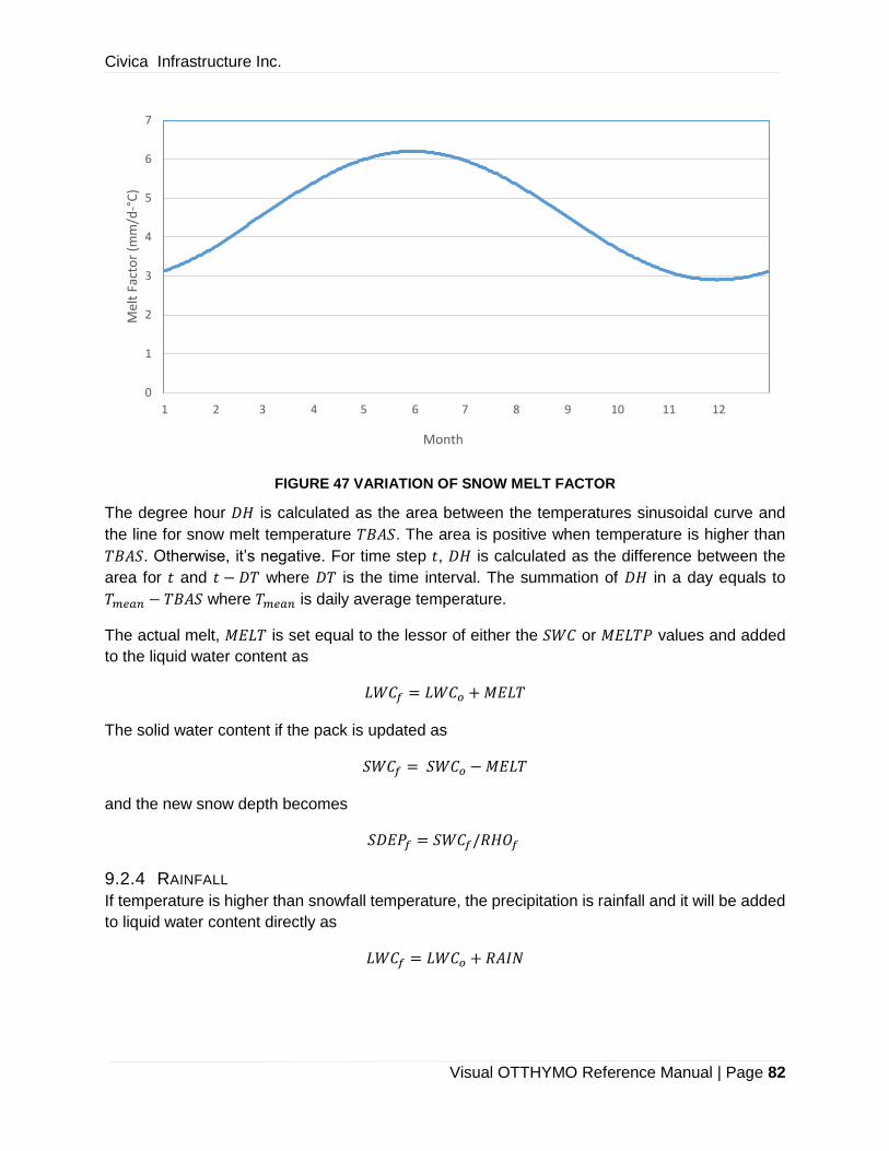
Civica Infrastructure Inc.
Visual OTTHYMO Reference Manual | Page 82
FIGURE 47 VARIATION OF SNOW MELT FACTOR
The degree hour 𝐷𝐻 is calculated as the area between the temperatures sinusoidal curve and
the line for snow melt temperature 𝑇𝐵𝐴𝑆. The area is positive when temperature is higher than
𝑇𝐵𝐴𝑆. Otherwise, it’s negative. For time step 𝑡, 𝐷𝐻 is calculated as the difference between the
area for 𝑡 and 𝑡 − 𝐷𝑇 where 𝐷𝑇 is the time interval. The summation of 𝐷𝐻 in a day equals to
𝑇𝑚𝑒𝑎𝑛 − 𝑇𝐵𝐴𝑆 where 𝑇𝑚𝑒𝑎𝑛 is daily average temperature.
The actual melt, 𝑀𝐸𝐿𝑇 is set equal to the lessor of either the 𝑆𝑊𝐶 or 𝑀𝐸𝐿𝑇𝑃 values and added
to the liquid water content as
𝐿𝑊𝐶𝑓 = 𝐿𝑊𝐶𝑜 + 𝑀𝐸𝐿𝑇
The solid water content if the pack is updated as
𝑆𝑊𝐶𝑓 = 𝑆𝑊𝐶𝑜 − 𝑀𝐸𝐿𝑇
and the new snow depth becomes
𝑆𝐷𝐸𝑃𝑓 = 𝑆𝑊𝐶𝑓/𝑅𝐻𝑂𝑓
9.2.4 RAINFALL
If temperature is higher than snowfall temperature, the precipitation is rainfall and it will be added
to liquid water content directly as
𝐿𝑊𝐶𝑓 = 𝐿𝑊𝐶𝑜 + 𝑅𝐴𝐼𝑁
0
1
2
3
4
5
6
7
1 2 3 4 5 6 7 8 9 10 11 12
Mel
t Fa
cto
r (m
m/d
-°C
)
Month
Civica Infrastructure Inc.
Visual OTTHYMO Reference Manual | Page 83
9.2.5 REFREEZE OF SNOWPACK LIQUID WATER
During periods of below freezing temperature, liquid water in the pack will refreeze thereby in-
creasing the solid water content. The potential amount of refreeze during a given time interval is
calculated using a temperature index method similar to snowmelt.
𝑅𝐸𝐹𝑅𝑍𝑃 =𝐾𝐹
24∗ 𝐷𝐻 𝑓𝑜𝑟 𝑇 ≤ 𝑇𝐵𝐴𝑆
𝑅𝐸𝐹𝑅𝑍𝑃 = 0 𝑓𝑜𝑟 𝑇 > 𝑇𝐵𝐴𝑆
where:
𝑅𝐸𝐹𝑅𝑍𝑃 = the amount of refreeze (mm);
𝐾𝐹 = the refreeze factor which is usually set equal to 𝐾𝑀.
The actual refreeze, 𝑅𝐸𝐹𝑅𝑍 (mm) is set equal to either 𝑅𝐸𝐹𝑅𝑍𝑃 or the current 𝐿𝑊𝐶, whichever is
less. Then the water balance of the pack is updated as follows.
𝐿𝑊𝐶𝑓 = 𝐿𝑊𝐶𝑜 − 𝑅𝐸𝐹𝑅𝑍
𝑆𝑊𝐶𝑓 = 𝑆𝑊𝐶𝑜 + 𝑅𝐸𝐹𝑅𝑍
The snow pack dry density 𝑅𝐻𝑂 is then updated.
9.2.6 SNOWPACK COMPACTION
As snow accumulates, it settles or compacts under its own weight, or by the action of the wind,
resulting in an increase in the dry density and a decrease in the porosity. A growth curve approach
was chosen to compute compaction effects. The new relative dry density, 𝑇𝑅𝐻𝑂 after an interval
of 𝐷𝑇 hours is determined as
𝑇𝑅𝐻𝑂 = 𝑅𝐻𝑂 ∗ 𝑀𝑅𝐻𝑂
𝑅𝐻𝑂 + (𝑀𝑅𝐻𝑂 − 𝑅𝐻𝑂) ∗ exp (−𝐷𝑇/𝐾𝐶)
𝐾𝐶 = 𝐵 ∗ exp (𝐴 ∗ 𝑇)
where:
𝑀𝑅𝐻𝑂 = the maximum specified relative dry density,
𝐾𝐶 = the compaction time constant (h),
𝐴 (1/°C) and 𝐵 (h) are coefficients.
Similar to 𝐾𝑀 and 𝑇𝐵𝐴𝑆, the seasonal variation is also applied to 𝑀𝑅𝐻𝑂.
The final dry density (due to compaction) for the interval 𝐷𝑇 is determined according to
𝑅𝐻𝑂𝑓 = 𝑅𝐻𝑂𝑜 𝑓𝑜𝑟 𝑇𝑅𝐻𝑂 ≥ 𝑀𝑅𝐻𝑂
𝑅𝐻𝑂𝑓 = 𝑇𝑅𝐻𝑂𝑜 𝑓𝑜𝑟 𝑇𝑅𝐻𝑂 < 𝑀𝑅𝐻𝑂
Civica Infrastructure Inc.
Visual OTTHYMO Reference Manual | Page 84
The snowpack depth is also updated with new dry density.
9.2.7 RELEASE OF LIQUID WATER
The maximum amount of liquid water that can be held in the pore spaces of a snowpack by
capillary forces is referred to as the liquid water holder capacity, 𝐿𝑊𝐶𝐴𝑃 and is computed using
𝐿𝑊𝐶𝐴𝑃 = 𝑃𝑂𝑅 ∗ 𝑆𝑊𝐼 ∗ 𝑆𝐷𝐸𝑃
Where 𝑆𝑊𝐼 is the irreducible water saturation and is expressed as a fraction of the total pore
volume.
Any liquid water in excess of the holding capacity will be released from the pack, therefore
𝑅𝑈𝑁𝑂𝐹𝐹_𝑆𝑁𝑂𝑊 = 𝐿𝑊𝐶𝑜 − 𝐿𝑊𝐶𝐴𝑃 𝑓𝑜𝑟 𝐿𝑊𝐶𝑜 > 𝐿𝑊𝐶𝐴𝑃
𝑅𝑈𝑁𝑂𝐹𝐹_𝑆𝑁𝑂𝑊 = 0 𝑓𝑜𝑟 𝐿𝑊𝐶𝑜 ≤ 𝐿𝑊𝐶𝐴𝑃
and 𝐿𝑊𝐶𝑓 is then set equal to 𝐿𝑊𝐶𝐴𝑃.
The values of 𝑅𝑈𝑁𝑂𝐹𝐹_𝑆𝑁𝑂𝑊 for each time step provide input to IA routine.
9.3 DEPRESSION STORAGE WATER BALANCE
The liquid water released from snow pack flows into depression storage first. It will first fill the
available storage and then flow out. The storage is then restored through evaporation and infiltra-
tion (in pervious area).
𝑅𝑈𝑁𝑂𝐹𝐹𝐼𝐴 = 𝑆𝑇𝑂𝑅𝑜 + 𝑅𝐴𝐼𝑁 + 𝑀𝐸𝐿𝑇 − 𝐸𝑇𝐼𝐴 − 𝐼𝑁𝐹𝐼𝐿 − 𝑆𝑇𝑂𝑅𝑚𝑎𝑥
𝑓𝑜𝑟 𝑆𝑇𝑂𝑅𝑜 + 𝑅𝐴𝐼𝑁 + 𝑀𝐸𝐿𝑇 − 𝐸𝑇𝐼𝐴 − 𝐼𝑁𝐹𝐼𝐿 > 𝑆𝑇𝑂𝑅𝑚𝑎𝑥
𝑅𝑈𝑁𝑂𝐹𝐹𝐼𝐴 = 0 𝑓𝑜𝑟 𝑆𝑇𝑂𝑅𝑜 + 𝑅𝐴𝐼𝑁 + 𝑀𝐸𝐿𝑇 − 𝐸𝑇𝐼𝐴 − 𝐼𝑁𝐹𝐼𝐿 ≤ 𝑆𝑇𝑂𝑅𝑚𝑎𝑥
where:
𝑅𝑈𝑁𝑂𝐹𝐹𝐼𝐴 = the amount of water flow out of depression storage (mm),
𝑆𝑇𝑂𝑅𝑜 = the initial amount of water stored in depression storage (mm),
𝐸𝑇𝐼𝐴 = the amount of water lost through evaporation (mm),
𝐼𝑁𝐹𝐼𝐿 = the amount of water infiltrates to active soil zone (mm)
𝑆𝑇𝑂𝑅𝑚𝑎𝑥 = the storage capacity (mm).
Then the water held in the storage is updated.
The evaporation 𝐸𝑇𝐼𝐴 is calculated with upper limit set to PET. The infiltration 𝐼𝑁𝐹𝐼𝐿 is only con-
sidered in pervious area and it’s calculated with given infiltration ratio as
𝐼𝑁𝐹𝐼𝐿 = 𝑆𝑇𝑂𝑅𝑜 ∗ 𝑅𝐴𝑇𝐼𝑂

Civica Infrastructure Inc.
Visual OTTHYMO Reference Manual | Page 85
9.4 ACTIVE SOIL ZONE WATER BALANCE
The water balance in active soil zone (pervious area) is simulated as
𝑆𝑆𝑇𝑂𝑅𝑓 = 𝑆𝑆𝑇𝑂𝑅𝑜 + 𝑅𝑈𝑁𝑂𝐹𝐹𝐼𝐴 + 𝐼𝐶𝑅𝑂 − 𝑅𝑈𝑁𝑂𝐹𝐹 − 𝐸𝑇 − 𝐺𝑊𝐼
where:
𝑆𝑆𝑇𝑂𝑅𝑓 = the amount of water stored in soil (mm),
𝑆𝑆𝑇𝑂𝑅𝑜 = the initial amount of water in soil (mm),
𝑅𝑈𝑁𝑂𝐹𝐹𝐼𝐴 = the runoff from depression storage (mm),
𝐼𝐶𝑅𝑂 = the effective runoff from indirectly connected impervious land surfaces
(mm),
𝑅𝑈𝑁𝑂𝐹𝐹 = surface runoff (mm),
𝐸𝑇 = the evapotranspiration (mm)
𝐺𝑊𝐼 = groundwater infiltration (mm).
9.4.1 WATER CONTRIBUTED FROM INDIRECTLY CONNECTED IMPERVIOUS AREA
𝐼𝐶𝑅𝑂 is the net contribution of water from impervious surfaces onto pervious surfaces referred to
as ‘indirectly connected impervious areas’. This net factor accounts for several physical conditions
reduce the impacts of indirectly connected impervious areas on pervious areas.
▪ Unlike precipitation and snowmelt, which are generally uniformly distributed over the per-
vious areas, runoff distribution from impervious areas are often concentrated in flow chan-
nels.
▪ Indirectly connected impervious areas are not always uniformly distributed over the entire
basin and only affect a fraction of the pervious surfaces.
The net effect is that water from indirectly connected areas is somewhat reduced and not available
over the entire pervious surfaces. This is modeled with a reduction factor in Continuous OT-
THYMO. Evaluation of typical lot layouts and grading suggest that a 0.20 multiplication factor
(80% reduction) of the indirectly connected areas is a reasonable value.
9.4.2 RUNOFF
The surface runoff 𝑅𝑈𝑁𝑂𝐹𝐹 is calculated using modified SCS equation
𝑅𝑈𝑁𝑂𝐹𝐹 = (𝑅𝑈𝑁𝑂𝐹𝐹𝐼𝐴 + 𝐼𝐶𝑅𝑂)2
𝑅𝑈𝑁𝑂𝐹𝐹𝐼𝐴 + 𝐼𝐶𝑅𝑂 + 𝑆𝑎𝑣
where 𝑆𝑎𝑣 is the available storage in active soil zone (mm) calculated as
𝑆𝑎𝑣 = 𝑆𝑚𝑎𝑥 − 𝑆𝑆𝑇𝑂𝑅 𝑤ℎ𝑒𝑛 𝑠𝑛𝑜𝑤𝑝𝑎𝑘𝑐 𝑑𝑜𝑒𝑠𝑛′𝑡 𝑒𝑥𝑖𝑠𝑡
𝑆𝑎𝑣 = (𝑆𝑚𝑎𝑥 − 𝑆𝑆𝑇𝑂𝑅) ∗ 𝑆𝑅𝐸𝐷𝑈𝐶𝑇 𝑤ℎ𝑒𝑛 𝑠𝑛𝑜𝑤𝑝𝑎𝑘𝑐 𝑒𝑥𝑖𝑠𝑡𝑠
where 𝑆𝑚𝑎𝑥 is the maximum available storage in active soil zone (mm) which is calculated with
curve number for antecedent moisture condition I (𝐶𝑁𝐼) as

Civica Infrastructure Inc.
Visual OTTHYMO Reference Manual | Page 86
𝑆𝑚𝑎𝑥 = (25400
𝐶𝑁𝐼− 254) /0.85
It’s assumed that soil is saturated (reaches to total porosity) when the amount of soil water equals
to 𝑆𝑚𝑎𝑥. 𝐶𝑁𝐼 is calculated from 𝐶𝑁𝐼𝐼 with
𝐶𝑁𝐼 =𝐶𝑁𝐼𝐼
2.3 − 0.013 ∗ 𝐶𝑁𝐼𝐼
The effective soil storage is adjusted during winter conditions in the presence of a snowpack with
a reduction factor 𝑆𝑅𝐸𝐷𝑈𝐶𝑇. This factor simulates soil frozen conditions with an apparent reduc-
tion in available soil storage.
9.4.3 EVAPOTRANSPIRATION
A PET reduction factor, 𝑃𝐸𝑇𝐹𝐴𝐶𝑇, is employed to account for lower evaporation during days with
rain. The default value is 0.1.
𝐸𝑝_𝑟𝑎𝑖𝑛 = 𝐸𝑝 ∙ 𝑃𝐸𝑇𝐹𝐴𝐶𝑇 𝑓𝑜𝑟 𝑅𝐴𝐼𝑁 > 0
The potential evapotranspiration will first be fulfilled by the evaporation from depression storage
and then the active soil zone. The available potential evapotranspiration for active soil zone,
𝐸𝑝_𝑠𝑜𝑖𝑙 is calculated as
𝐸𝑝_𝑠𝑜𝑖𝑙 = 𝐸𝑝_𝑟𝑎𝑖𝑛 − 𝐸𝑇𝐼𝐴
The ET rate from the active soil zone is calculated using the approach employed in Stanford
Watershed Model for ET from lower soil zone (Warren Viessman, 1977), which is
𝐸𝑇𝑠𝑜𝑖𝑙 = 𝐸𝑝𝑠𝑜𝑖𝑙−
𝐸𝑝𝑠𝑜𝑖𝑙
2
2𝑟 𝑓𝑜𝑟 𝐸𝑝𝑠𝑜𝑖𝑙
≤ 𝑟
𝐸𝑇𝑠𝑜𝑖𝑙 = 𝑟/2 𝑓𝑜𝑟 𝐸𝑝𝑠𝑜𝑖𝑙 > 𝑟
where 𝑟 is the evapotranspiration opportunity representing the maximal amount of water available
for evapotranspiration at a particular location. It’s calculated as
𝑟 = 𝐾3 ∙𝐿𝑍𝑆
𝐿𝑍𝑆𝑁
where:
𝐿𝑍𝑆 = the current soil moisture storage (mm),
𝐿𝑍𝑆𝑁 = a nominal storage level (mm)
𝐾3 = an input parameter that is a function of watershed cover as shown in Table 10.
In continuous OTTHYMO, 𝐿𝑍𝑆 is set equal to 𝑆𝑆𝑇𝑂𝑅 and 𝐿𝑍𝑆𝑁 is set to 𝑆𝑚𝑎𝑥/2.
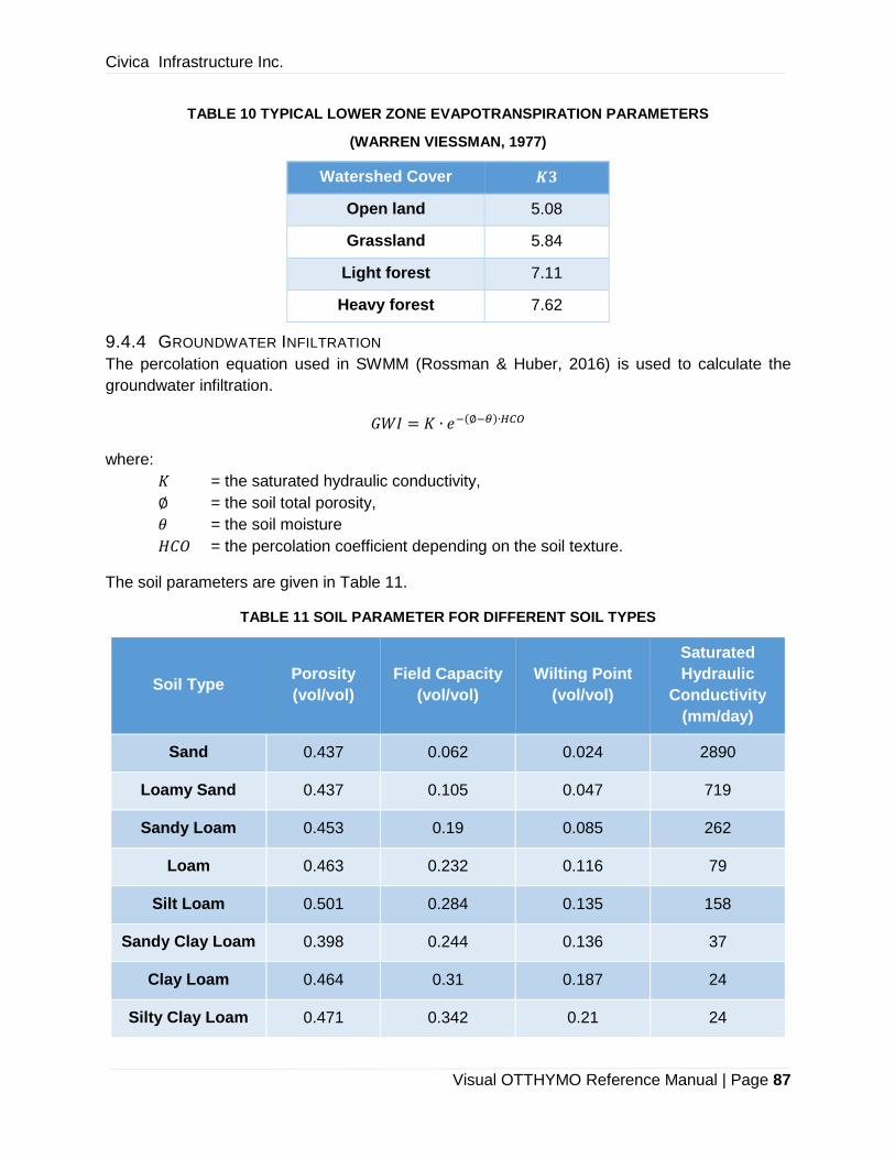
Civica Infrastructure Inc.
Visual OTTHYMO Reference Manual | Page 87
TABLE 10 TYPICAL LOWER ZONE EVAPOTRANSPIRATION PARAMETERS
(WARREN VIESSMAN, 1977)
Watershed Cover 𝑲𝟑
Open land 5.08
Grassland 5.84
Light forest 7.11
Heavy forest 7.62
9.4.4 GROUNDWATER INFILTRATION
The percolation equation used in SWMM (Rossman & Huber, 2016) is used to calculate the
groundwater infiltration.
𝐺𝑊𝐼 = 𝐾 ∙ 𝑒−(∅−𝜃)∙𝐻𝐶𝑂
where:
𝐾 = the saturated hydraulic conductivity,
∅ = the soil total porosity,
𝜃 = the soil moisture
𝐻𝐶𝑂 = the percolation coefficient depending on the soil texture.
The soil parameters are given in Table 11.
TABLE 11 SOIL PARAMETER FOR DIFFERENT SOIL TYPES
Soil Type Porosity
(vol/vol)
Field Capacity
(vol/vol)
Wilting Point
(vol/vol)
Saturated
Hydraulic
Conductivity
(mm/day)
Sand 0.437 0.062 0.024 2890
Loamy Sand 0.437 0.105 0.047 719
Sandy Loam 0.453 0.19 0.085 262
Loam 0.463 0.232 0.116 79
Silt Loam 0.501 0.284 0.135 158
Sandy Clay Loam 0.398 0.244 0.136 37
Clay Loam 0.464 0.31 0.187 24
Silty Clay Loam 0.471 0.342 0.21 24

Civica Infrastructure Inc.
Visual OTTHYMO Reference Manual | Page 88
Soil Type Porosity
(vol/vol)
Field Capacity
(vol/vol)
Wilting Point
(vol/vol)
Saturated
Hydraulic
Conductivity
(mm/day)
Sandy Clay 0.43 0.321 0.221 12
Silty Clay 0.479 0.371 0.251 12
Clay 0.475 0.378 0.265 6

Civica Infrastructure Inc.
Visual OTTHYMO Reference Manual | Page 89
REFERENCE
1. Arnell Viktor, "Rainfall Data for the design of Sewer Pipe Systems" Report Series A:8,
Department of Hydraulics, Chalmers University of Technology, 1982.
2. Arnell Viktor, "Analysis of Rainfall Data for use in Design of Storm Sewer Systems" Proc.
of the International Conference on "Urban Storm Drainage", University of Southhampton, Pentech
Press, London, April 1978
3. Bandyopadhyay M. "Synthetic Storm Pattern and Runoff for Gauhati India", Journal of the
Hydraulics Division, Proc. ASCE, vol.98, No.HY5, May 1972,pp 845-857.
4. Chow V.T. 'Handbook of Applied Hydrology', McGraw-Hill, New York, 1964.
5. Cronshey R.G. U.S. S.C.S "Synthetic Regional Rainfall Distributions", International Sym-
posium on Rainfall Runoff Modelling.
6. Department of Environment National Water Council Standing Commitee Reports No. 28
"Design and analysis of Urban Storm Drainage : The Wallingford Procedure vol. 1 "Principles,
Methods and Practice", September 1981.
7. Haan C.T. "Urban Runoff Hydrographs -Basic Principles" National Symposium On Urban
Hydrology, Hydraulics and Sediment Control.(University Of Kentucky, Lexington, Kentucky. July
26-29, 1976.)
8. Hogg W.D. "Time distribution of Short duration rainfall in Canada", Proceedings Canadian
Hydrology Symposium, Toronto, May 26-27, 1980 pp 53-63.
9. Huff F.A. "Time Distribution Of Rainfall In Heavy Storms" Water Resources Research, vol.
3, no.4, 1967, pp 1007-1019.
10. Keifer C. J. and Chu H.H. "Synthetic Storm Pattern For Drainage Design", Journal Of The
Hydraulics Division, proc. ASCE, vol. 83, no.HY4,August 1957,pp.
11. Kidd C.H.R. and Packmann J.C. "Selection Of Design Storm And Antecedent Condition
For Urban Drainage Design" Institute Of Hydrology Report No. 61, Wallingford, Avon, 1968.
12. McLarens J.F. Ltd. "A Comparison of Historical and Theoretical Design Storms for the City
of Edmonton", May 1979
13. Mcpherson M.B. "Synthetic Storm Pattern For Drainage Design" Discussion, Journal Of
The Hydraulics Division, proc. ASCE, vol 84,no. HY 1,1958,pp 49-57.
14. McPherson M.B. "Some Notes On The Rational Method Of Storm Drainage Design",
ASCE, Urban Water Resources Research Program. Tech Memo No. 6 (1969).
15. McPherson M.B. "The Design Storm Concept" Institute On Storm Water Detention Design,
University Of Wisconsin, Madison, Wisconsin, 1977.

Civica Infrastructure Inc.
Visual OTTHYMO Reference Manual | Page 90
16. Marsalek J. "Synthesized and Historical System For Urban Drainage Design" Proc. Of The
International Conference On Urban Storm Drainage, University of Southhampton, Pentech Press,
London, April 1978
17. Marsalek J. "Research on the Design Storm Concept" ASCE, Urban Water Resources
Research Program, Tech. Memo No.33, New York (1978).
18. National Environment Research Council "Flood Studies Report, vol.2 Meteorological Stud-
ies", NERC, London 1975.
19. Packmann J.C. and Kidd C.H.R. "A Logical Approach To The Design Storm Concept"
Water Resources Research, vol.16, No. 6, December 1980, pp 994- 1000.
20. Patry G. and Mcpherson M.B. "The Design Storm Concept" Proceedings of a Seminar at
Ecole Polytechnique de Montreal, May 1979, Montreal Quebec, December 1979.
21. Pilgrim D.H. and Cordery I. "Rainfall Temporal Patterns for Design Floods", Journal Of
The Hydraulics Division, proc. ASCE, vol. 101, No. HYI, 1975, pp 81- 95.
22. Terstriep M. and Stall J.B. "The Illinois Urban Drainage Area Simulator" Illinois State Water
Survey, Bulletin 58, Urbana Illinois, 1974.
23. U.S. Department of Agriculture, Soil Conservation Service, "A Method for Estimating Vol-
ume and Rate of Runoff in Small Watersheds" Technical Paper 149, Washington D.C. 1973.
24. Watson M.D. "Application of Illudas to Storm Water Drainage Design in South Africa" Re-
port No. 1/81 Urban Hydrology Series, Hydrological Research Unit, University Of Witwaterstrand,
Johannesburg, April, 1981.
25. Kibler D.F. ed. Urban Stormwater Hydrology, American Geophysical Union, Water Re-
sources Monograph 7. Washington D.C. 1982.
26. Wenzel H.G. and Voorhees M.L. "Sensitivity of Design Storm Frequency" in the Design
Storm Concept, Patry G. and Mcpherson M. B. eds., Proceedings of a Seminar at Ecole Poly-
technique Urban Water Resources Research Record Group. Ecole Polytechnique de Montreal.
GREMU-79/2, Montreal 1979.
27. Wisner P. and Gupta S. "Validity of Chicago Design Storms", Unpublished Paper, June
1980.
28. Wisner P. and Gupta S. "Preliminary Considerations on the Selection of Design Storms"
IMPSWM Progress Report No. 4, University of Ottawa, August 1979.
29. Yen B.C. and Chow V.T. "Design Hyetographs for Small Drainage Structures" Journal of
the Hydraulics Division, proc. ASCE, vol. 106, HY6, June 1980, pp 1055-1076.
30. Brunner, G. W., undated. Muskingum-Cunge Channel Routing.
Civica Infrastructure Inc.
Visual OTTHYMO Reference Manual | Page 91
31. Cunge, J.A., 1969. On the Subject of a Flood Propagation Computation Method (Musk-
ingum Method), Journal of Hydraulics Resources, Vol. 7, No.2, pp. 205-230.
32. Doan, W. P., 1994. Comparisons of Rainfall/Runoff Models for Two Watersheds in Colo-
rado, Urban Hydrology & Hydraulics Workshop, Davis, California.
33. Garbrecht, J. and Brunner, G., 1991. Hydrologic Channel Flow Routing for Compound
Sections, Journal of Hydraulic Engineering, Vol. 117, No. 5, pp. 629- 641.
34. Khan, H. 1993. Muskingum Flood Routing Model for Multiple Tributaries, Water Resources
Research, Vol. 29, No. 4, pp. 1057-1062.
35. Perumal, M., 1992. Multilinear Muskingum Flood Routing Method, Journal of Hydrology,
Vol. 133, pp. 259-272.
36. Ponce, V.M., 1978. Muskingum-Cunge Method with Variable Parameters, Journal of Hy-
draulics Division, ASCE, Vol. 104, No. HY12 Proc. Paper 14199, pp. 1663- 1667.
37. Ponce, V.M. and Theurer, F.D., 1982. Accuracy Criteria in Diffusion Routing, Journal of
Hydraulics Division, ASCE, Vol. 108, No. 6, pp. 747-757.
38. US Army Corps of Engineers, Hydrologic Engineering Center, 1994. Urban Hydrology &
Hydraulics Workshop, Davis, California.
39. Aaron, G.M., Miller, A.C., Lakatos, D.P. (1977), “Infiltration Formula Based on SCS Curve
Number,” Journal of Irrigation and Drainage Division, American Society of Civil Engineers, 103,
pp. 419-427.
40. *Alila, Y. (1988), “Selection of Routing Methods in Storm Sewers,” paper presented at the
International Symposium on Urban Hydrology and Municipal Engineering, Markham, Ontario,
June 13-15, 1988.
41. *Alila, Y., Wisner, P.E. (1989), “Verification of the New EXTRAN and the MOUSE Routing,
Advanced IMPSWM Research Program, Tech. Report No. 2, Department of Civil Engineering,
University of Ottawa, Ottawa, Canada.
42. Alley, W., Veenhuis, J.E. (1983), “Effective Impervious Area in Urban Runoff Modelling,
Journal of Hydraulic Engineering, Vol. 109, No. 2, February, 1983.
43. Altman, D.G., Espey, W.M., Feldman, A.R. (1980), “Investigation of Soil Conservation
Service Urban Hydrology Techniques,” presented at Canadian Hydrology Symposium, May 26-
27, 1980.
44. Beron P., Marchi, G. (1982), “SIRDU - An easy to use tool of analysis and design”, Urban
Drainage Systems, Pitman Advanced Program, London.
45. *Bryck, Jack M.G., Kelly, H., Bowins, D. (1986), “A Comparison of Modelled and Measured
Flows for McKenney Creek Drainage Basin,” Proceedings, Stormwater and Water Quality Man-
agement Modeling and SWMM Users Group Meeting, September 17-18, 1986, Toronto, Ontario.

Civica Infrastructure Inc.
Visual OTTHYMO Reference Manual | Page 92
46. *Calomino, F., Colosimo, C., Copertino, V.A., Veltri, P. (1983), “Modèle de crue dans un
petit bassin urbain : premiers résultats d'une recherche expérimentale” La houille blanche, No 2.
47. *Calomino, F., Veltri, P., Wisner, P. (1986), “Verifica di un semplice modello idrologico per
microcomputer sul basino urbano di Luzzi,” XX Convegno di Idraulica e Costruzioni Idrauliche,
Padova, 8-10 September 1986, pp. 497-508.
48. Calomino, F. (1988), “The Luzzi Watershed: Ten Years of Experience of Urban Runoff
Data Collection and Use,” paper presented at the International Symposium on Urban Hydrology
and Municipal Engineering, Markham, Ontario, June 13-15, 1988.
49. *Cebryk, R.S., Ouelette, J.G. (1986), “Experience with Master Drainage Planning in West-
ern Quebec,” Proceedings, Stormwater and Water Quality Management Modeling and SWMM
Users Group Meeting, September 17-18, 1986, Toronto, Ontario.
50. CH2MHILL, Inc. (1985), SAM: Wastewater Collection System Analysis Model User’s Man-
ual, Corvallis, Oregon 97339.
51. *Cheung, P. (1982), “A Standard Hydrograph Method for the Preliminary Analysis of
Stormwater Management Projects,” M.A.Sc. thesis, Department Of Civil Engineering, University
of Ottawa, Ottawa, Canada.
52. Chocat, B. (1984), “Conception, Evaluation et Dessin des Réseaux d'Egouts (CEDRE),”
Proceedings of the Third International Conference on Urban Storm Drainage, Volume 2, Gote-
borg, Sweden, June, 1984(a).
53. Chow, V.T. (1962), “Hydrologic Determination of Waterway Areas for the Design of Drain-
age Structures in Small Drainage Basins,” University of Illinois, Engineering Experiment Station
Bulletin No. 462.
54. Chow, V.T. (1964), “Runoff,” Section 14, Handbook of Applied Hydrology, McGraw-Hill.
55. Clarke, W. (1988), “Design Implications of Inlet Control,” paper presented at the Interna-
tional Symposium on Urban Hydrology and Municipal Engineering, Markham, Ontario, June 13-
15, 1988.
56. Clarke, W. (1988), “Rainfall Averaging for Lumped Catchment,” paper presented at the
International Symposium on Urban Hydrology and Municipal Engineering, Markham, Ontario,
June 13-15, 1988.
57. *Consuegra, D., Wisner, P. (1986), “Considerations on the Validation of a Model for Mas-
ter Drainage Plans,” Proceedings of the Conference on Urban Drainage Modelling and Compari-
son of Urban Drainage Models with Real Catchment Data, UDM 86, University of Belgrade, Per-
gamon Press, London.
58. *Consuegra, D. (1988), “Application of Regionalized Unit Hydrographs and Storm Water
Management Projects in Switzerland,” paper presented at the International Symposium on Urban
Hydrology and Municipal Engineering, Markham, Ontario, June 13-15, 1988.

Civica Infrastructure Inc.
Visual OTTHYMO Reference Manual | Page 93
59. *Consuegra, D., “Application du Modéle Hydrologique OTTHYMO et proposition pour son
application,” M.A.Sc. thesis, University of Ottawa, Ottawa, Canada.
60. Cunge, J.A., Holly, F.M., Verwey, A. (1981), Practical Aspects of Computational River
Hydraulics, Pitman, London.
61. *Da Silva, N.M., Wisner, P.E., Sabourin, J.F. (1988), “Numerical Experiments with Un-
steady Flow Simulations with EXTRAN model in a Large Conduit,” Report No. 86-12-9270, Na-
tional Laboratory of Civil Engineering, Lisbon, Proceedings, Celo< t< tna Konferencia so Zahrani<
nou, U< astou, Aktu< lne probl< me v Odkanalizovan< miest a priemyseln< ch z< vodov, Brati-
slava, 1989.
62. Danish Hydraulic Institute, Emolet Aps, PH-Consult Aps and I., Kruger A/S (1989),
“MOUSE User’s Guide and MOUSE Documentation,” MOUSE Service Gnter, Bregnevej 27, DK-
2820, Gentotte, Denmark.
63. Desbordes, M. (1978), “Urban Runoff and Design Storm Modelling in Urban Storm Drain-
age,” Proceedings of the International Conference, University of Southampton, ed. P.R. Helliwell,
Pentech Press, London, April, 1978.
64. Desbordes, M. (1975), “Estimation des coefficients de ruissellement urbains,” Universit<
des Sciences Techniques du Languedoc, France, Mars, 1975.
65. *Despotovic, J. (1988), “Statistical Analysis of Real Storms and Implications for the As-
sessment of a Past Flooding Event,” paper presented at the International Symposium on Urban
Hydrology and Municipal Engineering, Markham, Ontario, June 13-15, 1988.
66. Ding, J.Y. (1974), “Variable Unit Hydrograph,” Journal of Hydrology, Vol. 22, pp. 53-69.
67. Diskin, M.H. (1972), “The Role of Lag in a Quasi-Linear Analysis of the Surface Runoff
System,” Proceedings of the Second International Symposium in Hydrology, Colorado State Uni-
versity, Fort Collins, Colorado, September, 1972.
68. Diskin, M.H., Ince, S., Oben-Nyarko, K. (1978), “Parallel Cascades Model for Urban Wa-
tersheds,” Journal of the Hydraulics Division, ASCE, Vol. 104, No. Hy2, February, 1978, pp. 261-
276.
69. Dooge, J.C.I. (1973), “Linear Theory of Hydrologic System,” Technical Bulletin No. 1468,
Agricultural Research Service, U.S. Dept. of Agriculture, October 1973, p. 327.
70. Driscoll, D. (1983), “Rainfall/Runoff Relationships from the NURP Urban Runoff Data
Base,” paper presented at the Storm Water and Quality Models User’s Group Meeting, Montreal,
Quebec, 1983.
71. *El-Bahrawy, A. (1986), “OTTHYMO, User Manual,” Internal Report, Department of Civil
Engineering, University of Ottawa, Ottawa, Canada.

Civica Infrastructure Inc.
Visual OTTHYMO Reference Manual | Page 94
72. Espey, W., Jr., Altman, D.G., Graves, C.B., Jr. (1977), “Normographs for Ten- Minute Unit
Hydrographs for Small Urban Watersheds,” Appendum 3 of the ASCE Program Report Urban
Runoff Control Planning, June, 1977.
73. Foroud, N., Broughton, R.S. (1981), “Water Loss Equation and Coefficients to Estimate
Runoff from Rainfall,” Paper No. 80121 of the Water Resources Bulletin, Vol. 17, No. 3, June,
1981.
74. *Fraser, H.G. (1982), “Frequency of Storm Characteristics: Analysis and Implications for
Volume Design,” M.A.Sc. thesis, Department of Civil Engineering, University of Toronto, Toronto,
Canada.
75. *Fraser, H.G. (1988), “Modelling of Inflow/Infiltration Effects on a Large Sewerage Sys-
tem,of paper presented at the International Symposium on Urban Hydrology and Municipal Engi-
neering, Markham, Ontario, June 13-15, 1988.
76. Fuchs, L., Harms, R.W. (1986), “HYSTEM-EXTRAN Model Application in Scientific Inves-
tigations, Urban Drainage Modelling,” Proceedings of the International Symposium on Compari-
son of Urban Drainage Models with Real Catchment Data, UDM ‘86, Dubrovnik, Yugoslavia, Per-
gamon Press, New York.
77. *Gayer, J. (1988), “Application of Measurements on a Hungarian Watershed for the As-
sessment of System Schematization,” paper presented at the International Symposium on Urban
Hydrology and Municipal Engineering, Markham, Ontario, June 13-15, 1988.
78. Ghate, S.R., Whiteley, H.R. (1977), “GAWSER (Guelph Agricultural Watershed Storm-
Event Runoff) Model: User’s Manual,” University of Guelph, School of Engineering, Technical
Report 126-37.
79. *Gloor, R. (1983),”Application des mod< les OTTHYMO et HEC-2 au bassin versant de la
Seymaz,” paper presented at the Stormwater and Water Quality Models User’s Group Meeting,
Montreal, Quebec, 1983.
80. *Gloor, R., Wisner, P. (1984), “The Application of Microcomputers to the Calculation of
Design Flows and Flood Control, Microprocessors in operational Hydrology,” WMO, 1986, pp.
223-232.
81. *Gloor, R. (1988), “Flood and Runoff Control Near Geneva,” paper presented at the Inter-
national Symposium on Urban Hydrology and Municipal Engineering, Markham, Ontario, June
13-15, 1988.
82. Golding, B.C. (1979), “Runoff Curve Number with Varying Site Moisture,” Journal of Irri-
gation and Drainage Division, American Society of Civil Engineers, 105, pp. 434-441.
83. Golding, B.C. (1979), Discussion of “Runoff Curve Numbers with Varying Site Moisture,”
Journal of the Irrigation and Drainage Division, ASCE, Vol. 105, No. IR4, December, 1979.

Civica Infrastructure Inc.
Visual OTTHYMO Reference Manual | Page 95
84. Green, W.H., Ampt, G.A. (1911), “Studies on Soil Physics: I, Flow of Air and Water through
Soils,” Journal of Agr. Research, Vol. 4, pp. 1-24.
85. Harms, R.W. (1984), “Estimation of Runoff Volumes for Small Ungauged Urbanized
Catchments: in Analysis and Design of Stormwater Systems,” Proc. of the Third Intern. Confer-
ence on Urban Storm Drainage, Vol. 1, Goteborg, Sweden, June 4-8, 1984.
86. Harris, C.S. (1970), “Real Time Routing of Flood Hydrographs in Storm Sewers,”.J. of
Hyd. Div., ASCE, No. Hy6, pp. 7327.
87. Hawkins, R.H. (1978), “Runoff Curve Numbers with Varying Site Moisture,” Journal of the
Irrigation and Drainage Division, ASCE, Vol. 104, No. IR4, December, 1978, pp. 389-398.
88. Hogg, W.D. (1980), “Time Distribution of Short Duration Rainfall in Canada,” Proceedings,
Canadian Hydrology Symposium, Toronto, Ontario,May 26-27 , 1980, pp. 53-63.
89. Hogg, W.D. (1988), “Rainfall Data for the Urban Hydrologist,” paper presented at the In-
ternational Symposium on Urban Hydrology and Municipal Engineering, Markham, Ontario, June
13-15, 1988.
90. Holtan, H.N. (1961), “A Concept for Infiltration Estimates in Watershed Engineering,” ARS,
U.S. Dept. of Agriculture, Vol. 41, 1961.
91. Horton, R.E. (1933), “The Role of Infiltrataion in the Hydrologic Cycle,” Trans. Am. Ge-
ophys. Union, Vol. 14, pp. 446-460.
92. Huber, W.C., Heany, J.P., Nix, S.J., Dickinson, R.E., Polmann, D.J. (1982), “Storm Water
Management Model User’s Manual - Version III,” Municipal Environmental Research Centre, Of-
fice of Research and Development, U.S. Environmental Protection Agency, Cincinnati, Ohio, May,
1982.
93. Huber, W.C., Heany, J.P., Medina, M.A., Peltz, W.A., Sheikh, H., Smith, G.F. (1975),
“Storm Water Management User’s Manual - Version II,” Environmental Protection Technological
Series EPA-670-2-75-017, U.S. EPA, March, 1975.
94. Huber, W.C., Cunningham, B.A., Caender, K.A. (1986), “Continuous SWMM Modelling for
Selection of Design Events,” Int. Symp. on Comparison of Urban Drainage Models with Real
Catchment Data, Dubrovnik, Yugoslavia.
95. Islam, S. (1988), “Drainage and Runoff Water Problems of Dhaka, The Capital City of
Bangladesh,” paper presented at the International Symposium on Urban Hydrology and Municipal
Engineering, Markham, Ontario, June 13-15, 1988.
96. Jacobson, P., Harremoes, P. (1984), “The Significance of Head Loss Parameters in Sur-
charged Sewer Simulations,” Proceeding of the Third International Conference on Urban Storm
Drainage, Goteborg, Sweden, June 4-8, Vol. 1.

Civica Infrastructure Inc.
Visual OTTHYMO Reference Manual | Page 96
97. James F. MacLaren Ltd. (1975), “Review of Canadian Design Practice and Comparison
of Urban Hydrology Models,” Research Report No. 26, Canada- Ontario Agreement on Great
Lakes Water Ouality Project No. 74-8-31, October, 1975.
98. *Jaton, J.F. (1983), “< tude monographique succinte du bassin versant du Parimbot,” Pub-
lic, IGR No. 168, EPFL, Lausanne.
99. *Jobin, D.I. (1982), “Application du mod< le OTTHYMO sur un basin exp< rimental en
Suisse,” Th< se M.Eng., D< partement de G< nie Civil, Universit< d’Ottawa, Ottawa, Canada.
100. *Jordan, J.P., Wisner, P.E. (1983), “Description du mod< le OTTHYMO et Exemples d’Ap-
plications,” < cole Polytechnique F< d< rale de Lausanne, IGR 172.
101. *Kassem, A. (1982), “Development and Application of a Simultaneous Routing Model for
Dual Drainage Systems,” Ph.D. thesis, Department of Civil Engineering, University of Ottawa,
Ottawa, Canada.
102. *Kassem, A. (1982), “Development and Application of a Simultaneous Model for Dual
Drainage Systems,” Ph.D. dissertation, Department of Civil Engineering, University of Ottawa,
Ottawa, Canada.
103. *Kassem, A., Wisner, P.E. (1983), “The OTTSWMM Model User Manual in Procedures
for Modelling of Urban Drainage Systems,” Department of Civil Engineering, University of Ottawa,
Ottawa, Canada.
104. Keifer, C.J., Chu, H.M. (1957), “Synthetic Storm Pattern for Drainage Design,” Journal of
the Hydraulic Division, ASCE, Vol. 83, No. HY4, August, 1957.
105. Kerby, W.S. (1959), “Time of Concentration for Overland Flow,” Civil Engineering, Vol. 29,
No. 3, p. 60, March, 1959.
106. Kibler, D.F. (1982), “Urban Stormwater Hydrology,” American Geophysical Union, Water
Resources Monograph No. 7, Washington, DC.
107. Kidd, C.H.R., editor (1978), “Rainfall-Runoff Processes Over Urban Surfaces,” Proceed-
ings of an International Workshop, Institute of Hydrology, Wallingford, Oxon, U.K., April, 1978.
108. Kidd, C.H.R., Packmann, J.C. (1978), “Selection of Design Storm and Antecedent Condi-
tion for Urban Drainage Design,” Institute of Hydrology, Report No. 61, Wallingford, Oxon, U.K.
109. Kouwen, N. (1984), “An Adaptation of HYMO: Problem-Oriented Computer Language for
Hydrologic Modelling: HYMO-BASIC,” Water Resources Group, Department of Civil Engineering,
University of Waterloo, Ontario.
110. Lam, A. (1988), “Design of Small Storage Tanks for I/I Compensation,” paper presented
at the International Symposium on Urban Hydrology and Municipal Engineering, Markham, On-
tario, June 13-15, 1988.

Civica Infrastructure Inc.
Visual OTTHYMO Reference Manual | Page 97
111. Lam, A., Rampersad, C. (1986), “Interface of Lumped and Detailed Modelling,” Proceed-
ings, Stormwater and Water Quality Management Modeling and SWMM Users Group, Meeting,
September 17-18, 1986, Toronto, Ontario.
112. Lynch, J.A., Corbet, E.S. (1982), “Relationship of Antecedent Flow Rate to Storm Hydro-
graph Components,” presented at International Symposium on Hydrometeorology, Am. Water
Res. Association, June, 1982.
113. Mahmood, K., Yevjevich, V. (1975), “Unsteady Flow in Open Channels,” Vol. 1, Water
Resources Publications, Fort Collins, Colorado.
114. Marsalek, J. (1977), “Malvern Urban Test Catchment, Vol. I,” Research Report No. 57,
Canada-Ontario Agreement on Great Lakes Water Quality, Project No. 73-3- 12.
115. Marsalek, J. (1979), “Malvern Urban Test Catchment, Vol. II,” Research Report, No. 95,
Canada-Ontario Agreement on Great Lakes Water Quality, Project No. 73- 3-12.
116. Marsalek, J. (1978), “Synthesized and Historical Storms for Urban Drainage Design,” Pro-
ceedings of the International Conference on Urban Storm Drainage, University of Southampton,
Penetech Press, London, April, 1978.
117. Marsalek, J. (1980), “Sewer Inlets Study - Laboratory Investigation of Selected Inlets,”
Environmental Hydraulics Section, National Water Research Institute, Burlington, Ontario, July,
1980.
118. Marsalek, J., Watt, W.E. (1983), “Design Storms for Urban Drainage Design,” Proceed-
ings, 6th Canadian Hydrotechnical Conference, Ottawa, June, 1983.
119. Marsalek, J. (1988), “Considerations of Manhole Head Losses in Pressurized Sewer Flow
Routing,” paper presented at the International Symposium on Urban Hydrology and Municipal
Engineering, Markham, Ontario, June 13-15, 1988.
120. *Matos, M.R. (1988), “Experience with Rainfall-Runoff Measurements and Interpretation
in Portugal,” paper presented at the International Symposium on Urban Hydrology and Municipal
Engineering, Markham, Ontario, June 13-15, 1988.
121. *Matos, M.R. (1987), “Methods for Analysis and Evaluation of Peak Discharges in Urban
Drainage Systems - Study based on Data from Experimental Portuguese Catchments.” Thesis
prepared in partial fulfillment for the degree of specialist of LNEC, Lisbon.
122. *Matos, M.R., Silva, M.H. (1986), “Experiences from Stormwater Modelling in Portugal
with Real Catchment Data,” Proc. International Symposium on Comparison of Urban Drainage
Models with Real Catchment Data, Dubrovnik.
123. Maskimovic, C., Radojkovic, M. (1986), Urban Drainage Catchments, Selected Worldwide
Rainfall Data from Experimental Catchments, University of Belgrade, Yugoslavia, Pergamon
Press, Yugoslavia.

Civica Infrastructure Inc.
Visual OTTHYMO Reference Manual | Page 98
124. *Maza, J. (1988), “Inadequate Capacity of a Ditch Drainage System and Remedial
Measures in the City of Rivadavia (Argentina),” paper presented at the International Symposium
on Urban Hydrology and Municipal Engineering, Markham, Ontario, June 13-15, 1988.
125. *Mignosa, P., Paoletti, A. (1988), “Model Calibration and Application on Large Urban Ar-
eas with Non-Uniform Storm Distribution,” paper presented at the International Symposium on
Urban Hydrology and Municipal Engineering, Markham, Ontario, June 13-15, 1988.
126. *Mignosa, P., Paoletti, A., Tanda, M.G. (1984), “Application of OTTHYMO Model to the
Milano’s Sewer System, 3rd Int. Conf. on Urban Storm Drainage, Goteborg, Sweden.
127. Miller, R.A. (1979), “The Hydraulic Effective Impervious Area of an Urban Basin, Broward
County, Florida,” presented at the International Symposium on Urban Storm Water Management,
University of Kentucky, Lexington, Ky, July, 1979.
128. Minshall, N.E. (1960), “Predicting Storm Runoff on Small Experimental Watersheds,” Jour-
nal of Hydraulics Division, ASCE 86 (HY6), pp. 17- 28.
129. Mirza M. (1986), Proceedings of the First Canadian Conference on Computer Applications
in Civil Engineering/Microcomputers, editor, McMaster University, Hamilton, Ontario, Canada.
130. Musy, A. (1974), “Contribution < 1’< tude des < coulements en milieux non satur< s,” Th<
se EPFL, Lausanne.
131. Nash, J.E. (1957) “The Form of the Instantaneous Hydrograph,” International Association
of Scientific Hydrology, Publication 45, pp. 114-121.
132. Niemczynovicz, J. (1988), “Moving Storms as an Areal Input to Runoff Simulations Mod-
els,” paper presented at the International Symposium on Urban Hydrology and Municipal Engi-
neering, Markham, Ontario, June 13-15, 1988.
133. Nix, S.J., Heany, J.P., Huber, W.C. (1978), “Revised SWMM Storage Treatment Block,”
Proceedings, SWMM Users Meeting EPA-600-9-79-003, November, 1978.
134. Ontario Ministry of Natural Resources (1983), VUH Model User’s Manual, Conservation
Authorities and Water Management Branch, Toronto, Ontario, July, 1983.
135. Ontario Ministry of Transportation and Communications (1982), “Design Flood Estimates
for Small Watersheds,” MTC Drainage Manual, Chapter B.
136. Ontario Ministry of Transportation and Communications (1981), “Hydraulic Design of
Storm Sewers,” MTC Drainage Manual, Chapter E, Draft by Proctor & Redfern Ltd., April, 1981.
137. Ontario Ministry of Transportation and Communications (1982), “Design Flood Estimation
for Medium and Large Drainage Basins in Ontario,” Bridge Hydrology Series No. 2.
138. Overton, D.E., Meadows, M.E. (1976), Storm water Modelling, Academic Press, New
York.

Civica Infrastructure Inc.
Visual OTTHYMO Reference Manual | Page 99
139. *Pankratz, R. (1986), “Limitations of Single Event Modelling for Design of Detention Ponds
with Small Release Rates,” Proceedings of the Storm Water and Water Quality Modelling Users
Meeting, edited by P. Wisner, Toronto.
140. *Paoletti, A. (1984), “Gli Studi Spermentali Di Pavia e Milano, Seminario Sui delflussi Ur-
bani, Cosenza.
141. Papadakis, C.N., Preal, H.C. (1972), “Urban Runoff Characteristics,” Report No. 11024,
DQU, Environmental Protection Agency, Washington.
142. Pedersen, J.T., Peters, J.C., Helweg, O.C. (1980), “Hydrographs by Single Linear Reser-
voir Model,” Journal of the Hydraulics Division, ASCE, Vol. 106, No. H5, Proc. Paper 15430, May,
1980.
143. *Pilon, P. (1988), “Comparison of Design Flood Methodologies on a Small Rural Water-
shed in Southern Ontario,” paper presented at the International Symposium on Urban Hydrology
and Municipal Engineering, Markham, Ontario, June 13-15, 1988.
144. *P’ng, C.E. (1982), “Conceptual Hydrologic Modelling for Master Plans in Urban Drain-
age,” M.A. thesis, Department of Civil Engineering, University of Ottawa, Ottawa, Canada.
145. *Preissman, A. (1961), “Propagation of Translatory Waves in Channels and Rivers,” in
Proceedings, First Congress of the French Association for Computation, Grenoble, France, pp.
433-442.
146. *Preul, R.C. and Papadakie (1972), “Urban Runoff Characteristics,” Report No. 11204,
DQU, Environmental Protection Agency, Washington.
147. Proctor & Redfern Ltd. and James F. MacLaren Ltd. (1976), “Storm Water Management
Model Study, Volume I,” Research Report No. 47, Canada-Ontario Agreement on Great Lakes
Water Quality, _Project No. 73-5-70, September, 1976.
148. Proctor & Redfern Ltd. and James F. MacLaren Ltd. (1976), “Storm Water Management
Model Study, Volume II,” Research Report No. 48, Canada-Ontario Agreement on Great Lakes
Water Quality, Project No. 73-5-10, September, 1976.
149. *Radu, M. (1988), “Stormwater Drainage Studies for Douala City in Cameroun A Systems
Approach,” paper presented at the International Symposium on Urban Hydrology and Municipal
Engineering, Markham, Ontario, June 13-15, 1988.
150. Rallison, R.E. (1979), “Discussion of ‘Runoff Curve Numbers with Varying Site Moisture’,”
Journal of Irrigation and Drainage Division, 105, pp. 439-441.
151. *Rampersad, C., Sabourin, J.F., Cheung, P. (1986), “Comparison of the IMPRAM Model
(Improved Rational Method) with Other Models,” Proceedings, Stormwater and Water Quality
Management Modeling and SWMM Users Group Meeting, September 17-18, 1986, Toronto, On-
tario.
Civica Infrastructure Inc.
Visual OTTHYMO Reference Manual | Page 100
152. Rao, A.R., Delleur, J.W., Sarma, P.B.S. (1972), “Conceptual Hydrologic Models for Ur-
banizing Basins,” Journal of the Hydraulics Division, ASCE, Vol. 92, No. HY7, Proc. Paper 9024,
pp. 1205-1220, July, 1972.
153. Rawls, J., Brakensiek, D., Miller, N. (1983), “Green-Ampt Infiltration Parameters from Soil
Data,” Journal of Hydraulic Engineering, Vol. 109, No. 1.
154. Roesner, L.A. et al. (1981), “Storm Water Management Model User’s Manual, Version III,
Addendum I, EXTRAN,” U.S. Environmental Protection Agency, Cincinnati, Ohio.
155. *Rowney, A.C. (1985), “CONTHYMO - A Continuous Simulation Model for Regional
Stormwater Management Planning Analysis,” Ph.D. thesis, Department of Civil Engineering, Uni-
versity of Ottawa, Ottawa, Canada.
156. *Rowney, A.C., Wisner, P. (1985), “QUALHYMO - An Alternative Continuous Quality
Quantity Simulation Model,” Proceedings of the Conference on Stormwater and Water Quality
Modelling, edited by W. James, Toronto, Canada.
157. *Sabourin, J.F. (1988), “Importance of the UDM Rainfall Runoff Measurements for the
Municipal Engineer,” paper presented at the International Symposium on Urban Hydrology and
Municipal Engineering, Markham, Ontario, June 13-15, 1988.
158. *Sabourin, J.F., “Contribution to the Updating and Expansion of OTTHYMO, M.Eng. pro-
ject, University of Ottawa, Ottawa, Canada.
159. Sarma, P.B.S., Delleur, J.W., Rao, A.R. (1972), “Comparison of Rainfall-Runoff Models
for Urban Areas,” Journal of Hydrology, 18, pp. 329-347.
160. *Scholl, J. (1988), “The Need for Modelling Improvements and Examples from USA Stud-
ies,” paper presented at the International Symposium on Urban Hydrology and Municipal Engi-
neering, Markham, Ontario, June 13-15, 1988.
161. Schulze, R.E. (1984), “Hydrological Models for Application to Small Rural Catchments in
Southern Africa: Refinements and Development,” Report to the Water Research Commission by
the Department of Agricultural Engineering, University of Natal, South Africa.
162. Smith, A. (1986), “Incorporating the SWMM/Runoff Algorithm in a Design Program,” Pro-
ceedings of the Storm Water and Water Quality Modelling Users Meeting, edited by P. Wisner,
Toronto.
163. Soil Conservation Service (1971), National Engineering Handbook, Section 4, Hydrology,
U.S. Department of Agriculture, U.S. Government Printing Office, Washington, DC.
164. Soil Conservation Service (1975), “Urban Hydrology for Small Watersheds,” Technical
Release No. 55, U.S. Dept. of Agriculture, January, 1975.
165. Stall, J.B., Terstriep, M.L. (1979), “The Illinois Urban Drainage Area Simular (ILLUDAS),”
State Water Survey Division of Illinois, Urbana Bulletin 58, Urbana, U.S.A.
Civica Infrastructure Inc.
Visual OTTHYMO Reference Manual | Page 101
166. Stone, D. (1988), “Ecological Aspects for the Design of a SWM Storage,” paper presented
at the International Symposium on Urban Hydrology and Municipal Engineering, Markham, On-
tario, June 13-15, 1988.
167. Torno, M. (1985), Proceedings of the Specialty Conference on Computer Applications in
Water Resources, editor: American Society of Engineering, ASCE, Buffalo, N.Y.
168. Townsend, D.R., Wisner, P., Moss, D.J. (1980), “Inlet Control Devices for Storm Water
Catchbasins, A Laboratory Study,” presented at Canada Hydrology Symposium 80, Toronto, On-
tario, May, 1980.
169. *Umble, Art K., Salcedo, L., “Town Branch Drainage Study,” Proceedings, Stormwater and
Water Quality Management Modeling and SWMM Users Group Meeting, September 17-18, 1986,
Toronto, Ontario.
170. *Vazquez, R. (1988), “Flood Relief Studies in Barcelona,” paper presented at the Interna-
tional Symposium on Urban Hydrology and Municipal Engineering, Markham, Ontario, June 13-
15, 1988.
171. Viessman, W., Miller, C.F. (1972), “Runoff Volumes from Small Urban Watersheds,” Water
Resources Research, Vol. 8, No. 2, April, 1972.
172. Viessman, W., Jr. (1966), “The Hydrology of Small Impervious Areas,” Water Resources
Research, Vol. 2, No. 3, pp. 405-412.
173. Viessman, W., Jr. (1968), “Runoff Estimation for Very Small Drainage Areas,” Water Re-
sources Research, Vol. 4, No. 1, February, 1968.
174. Willeke, C.E. (1966), “Time in Urban Hydrology,” Journal of the Hydraulics Division, ASCE,
Vol. 92, No. HY1, Proc. Paper 4615, January, 1966, pp. 13-29.
175. Williams, J.R., Hann, R.W. (1973), “HYMO - A Problem-Oriented Computer Language for
Hydrologic Modelling,” ARS-5-9, U.S. Dept. of Agriculture.
176. Williams, J.R. (1968), “Runoff Hydrograph from Small Texas Blacklands Watersheds,”
U.S. Dept. of Agriculture, Agricultural Research Service, ARS-41- 143, October, 1968, p. 24.
177. Williams, J.R. (1972), “Concept of a Technique for an Analysis of Watershed Runoff
Events,” Proceedings of the Second International Symposium in Hydrology, Colorado State Uni-
versity, Fort Collins,.Colorado, September, 1972.
178. *Wisner, P., Gloor, R., Lam, A. (1984), “Application des microordinateurs dans le contr<
le des inondations dans les petits bassins urbains,” Proceedings, World Meteorological Sympo-
sium on Microcomputer Applications in Operational Hydrology, Geneva, September, 1984.
179. *Wisner, P.E., Gupta, S., Kassem, A. (1980), “Considerations Regarding the Application
of SCS TR-55 Procedures for Runoff Computations,” Proceedings, SWMM User Group Meeting,
USEPA 600-9-80-064, pp. 23-44.

Civica Infrastructure Inc.
Visual OTTHYMO Reference Manual | Page 102
180. *Wisner, P.E., Kassem, A.M. (1980), “Review and Comparison of Routing Methods in
Storm Water Modelling,” IMPSWM Report No. 1, Department of Civil Engineering, University of
Ottawa, Ottawa, Canada, October, 1980.
181. *Wisner, P.E., Mukherjee, D., Keliar, D. (1980), “Implementation of Stormwater Manage-
ment in a Canadian Municipality: The Markham Experience with Site- Tailored Criteria,” in Storm-
water Management Alternatives, University of Delaware Resource Center, April, 1980.
182. *Wisner, P.E. (1982), “The IMPSWM Procedures for Urban Drainage Modelling and Some
Applications,” Proceedings, Stormwater and Water Quality Modeling and SWMM Users Group
Meeting, University of Ottawa, October 18-19, 1982.
183. *Wisner, P.E., Kassem, A.M. (1983), “OTTSWMM, A Model for the Analysis and Design
of Dual Drainage Systems,” Part IV, IMPSWM Urban Drainage Modelling, Procedures, 2nd Edi-
tion, Department of Civil Engineering, University of Ottawa, Ottawa, Canada, February, 1983.
184. *Wisner, P.E., P’ng, C.E. (1983), “OTTHYMO, A Model for Master Drainage Plans,” Part
III, IMPSWM Urban Drainage Modelling Procedures, 2nd Edition, Department of Civil Engineer-
ing, University of Ottawa, Ottawa, Canada.
185. *Wisner, P.E., Fraser, H. (1983), “Design Storms for Stormwater Management Studies,”
Part V, IMPSWM Urban Drainage Modelling Procedures, 2nd Edition, Department of Civil Engi-
neering, University of Ottawa, Ottawa, Canada, February, 1983.
186. *Wisner, P.E. (1983), “A Hierarchical Approach to Urban Hydrology Modelling: The
IMPSWM Methodology,” Proceedings of the International Symposium on Urban Runoff, Univer-
sity of Kentucky, Lexington, Kentucky, July, 1983.
187. *Wisner, P.E., Lam, A. (1983), “Twin Models for Storm Water Management Mainframe
Computers and Microcomputers,” ASCE Engineering Foundation Conference on Emerging Com-
puter Techniques in Stormwater and Flood Management, Niagara-on-the-Lake, Ontario, Canada,
Oct. 30 - Nov. 4, 1983.
188. *Wisner, P.E., Lam, A., Chin, N. (1983), “DUHYD - Development of Dual Drainage Sub-
model in OTTHYMO,” International Report, Department of Civil Engineering, University of Ottawa,
Ottawa, Canada.
189. *Wisner, P.E., Fraser, H., P’ng, C. (1983), “An Investigation of the VUH and OTTHYMO
Models,” Report to the Ontario Ministry of Natural Resources.
190. *Wisner, P.E., Lam, A., Rampersad, C. (1984), “Realistic Simulation of Sewer Surcharge
and Prevention of Basement Flooding,” Proceedings of the Conference on Urban Storm Drainage,
Goteborg, Sweden.
191. *Wisner, P. (1984), “Experience with the Implementation of Storm Water Management
Models,” Proceedings of the Conference on Urban Storm Drainage, Goteborg, Sweden.
Civica Infrastructure Inc.
Visual OTTHYMO Reference Manual | Page 103
192. *Wisner, P.E., Lam, A., Sabourin, J. (1984), “Development of a Multilevel Package of
Stormwater Management Models,” Proceedings, Conference on Microcomputers in Civil Engi-
neering, University of Florida, Orlando.
193. *Wisner, P., Consuegra, D., El-Bahrawy, A. (1986), “Calibration of Urban Hydrology Mod-
els by Trial and Error and Optimization,” Proceedings of the Storm Water and Water Quality Mod-
elling Users Meeting, edited by P. Wisner, Toronto, 1986(b).
194. *Wisner, P., Consuegra, D., Sabourin, J.F. (1986), “Role of Simplified Micro- Computer
Models as Parts of Multilevel Hydrological Packages,” Hydrosoft, Hydraulic Engineering Software,
International Conference, Southampton, U.K., 1986©.
195. *Wisner, P., Consuegra, D., Sabourin, J.F., Lam, A. (1986), “Simplified Microcomputer
Models as Part of Multilevel Package for Small Rural and Urban Watersheds,” Proceedings,
Stormwater and Water Quality Management Modeling and SWMM Users Group Meeting, Sep-
tember 17-18,1986, Toronto, Ontario.
196. *Wisner, P. and Consuegra, D. (1986), “Consideration on the Deterministic Simulation for
Pollution Control Studies,” Proceedings, Stormwater and Water Quality Management Modeling
and SWMM Users Group Meeting, September 17- 18, 1986, Toronto, Ontario.
197. *Wisner, P., Lam, A., Gloor, R. (1984), “Microcomputer Applications of an Urban Hydrol-
ogy Model,” 3rd Goteborg, 1984, Vol. 2, p. 523.
198. *Wisner, P.E., Despotovic, J. (1988), “Statistical Analysis of Real Storms and Implications
for the Assessment of a Past Flooding Event,” paper presented at the International Symposium
on Urban Hydrology and Municipal Engineering, June 13-15, 1988, Markham, Ontario, Canada.
199. *Wisner, P., Kassem, A., Sabourin, J.F., Alila, Y. (1989), “Numerical Experiments for the
Comparison of Routing Methods in Storm Sewers,” Recent Aspects of Storm Drainage and Sew-
erage of Residential and Industrial Areas.
200. Wittenberg, H. (1975), “A Model to Predict the Effects of Urbanization on Watershed Re-
sponse,” National Symposium on Urban Hydrology and Sediment Control, University of Kentucky,
Lexington, Kentucky, July 28-31, 1975.
201. Wright-McLaughlin Engineers (1968), Urban Storm Drainage Criteria Manual, Regional
Council of Governments, Denver, Colorado.
202. Yen, B.C. (1987), “Urban Drainage Hydraulics and Hydrology From Art to Science,” Urban
Drainage Hydraulics and Hydrology, Proc. Int. Conf. in Urban Storm Drainage, Lausanne, Swit-
zerland, Editor B.C. Yen.
203. Yen, B.C. (1986), “Hydraulics of Sewers,” Advances of Hydroscience, Founding Editor
V.T. Chow, Academic Press, pp. 1-122.

Civica Infrastructure Inc.
Visual OTTHYMO Reference Manual | Page 104
204. Yen, B.C. (1978), “Hydraulic Instabilities of Storm Sewer Flows in Urban Storm Drainage,”
Proc. Int. Conf. lst. (P.R. Belliveil, ed.), pp. 282-293, Pentech, Press, London and Wiley-Inter-
science, New York.