Visualizing and Understanding Deep Neural Networks in CTRPrediction

Lin GuoAlibaba Group

Hui YeAlibaba Group

Wenbo SuAlibaba Group

Henhuan LiuAlibaba Group

Kai SunAlibaba Group

Hang XiangAlibaba Group

ABSTRACTAlthough deep learning techniques have been successfully appliedto many tasks, interpreting deep neural network models is still abig challenge to us. Recently, many works have been done on visu-alizing and analyzing the mechanism of deep neural networks inthe areas of image processing and natural language processing. Inthis paper, we present our approaches to visualize and understanddeep neural networks for a very important commercial task—CTR(Click-through rate) prediction.We conduct experiments on the pro-ductive data from our online advertising system with daily varyingdistribution. To understand the mechanism and the performanceof the model, we inspect the model’s inner status at neuron level.Also, a probe approach is implemented to measure the layer-wiseperformance of the model. Moreover, to measure the influence fromthe input features, we calculate saliency scores based on the back-propagated gradients. Practical applications are also discussed, forexample, in understanding, monitoring, diagnosing and refiningmodels and algorithms.

ACM Reference format:Lin Guo, Hui Ye, Wenbo Su, Henhuan Liu, Kai Sun, and Hang Xiang. 2018.Visualizing and Understanding Deep Neural Networks in CTR Prediction.In Proceedings of ACM SIGIR Workshop on eCommerce, Ann Arbor, Michigan,USA, July 2018 (SIGIR 2018 eCom), 7 pages.https://doi.org/

1 INTRODUCTIONClick-through rate (CTR) prediction plays a crucial role in com-putational advertising. In the common cost-per-click advertisingsystem, advertisements are ranked by the product of the bid priceand the predicted CTR when bidding for impression opportunities.Therefore, the revenue of the multi-billion business heavily relieson the performance of the CTR prediction model.

Deep learning techniques have been successfully applied to CTRprediction tasks [6, 7, 23]. Deep neural networks (DNNs), composedof stacked layers of neurons, have the capability to extract thenonlinear patterns from features and thus reduce the burden ofnontrivial feature engineering. However, the working mechanismsof deep learning models are still not well understood. The lack of

Permission to make digital or hard copies of part or all of this work for personal orclassroom use is granted without fee provided that copies are not made or distributedfor profit or commercial advantage and that copies bear this notice and the full citationon the first page. Copyrights for third-party components of this work must be honored.For all other uses, contact the owner/author(s).SIGIR 2018 eCom, July 2018, Ann Arbor, Michigan, USA© 2018 Copyright held by the owner/author(s).ACM ISBN .https://doi.org/

interpretability becomes an obstacle for deep learning, and raisesconcerns on the reliability of deep learning applications, especiallyfor critical industrial implementations.

Many recent progresses have been made in visualizing and in-terpolating deep learning models for image processing [15, 18, 20,21, 26, 29] and natural language processing [3, 4, 14, 16, 27]. In thispaper, we present a series of approaches to visualize and analyze asimple DNN model for CTR prediction on the productive data fromour search advertising platform. The model’s performance decay isinvestigated over datasets with daily varying distribution, and thedistributions of the output scores are also compared for differenttraining stages. We inspect the model’s inner status down to neuronlevel. We study the statistical properties of the neurons’ statuses forthe hidden layers, and investigate the high-level representationslearned by the model through t-SNE projection [17, 21]. A probemethod [2] is applied to dissect model’s performance layer by layerfor different datasets. Moreover, to measure the influence of theinput features, we calculate saliency scores for the feature groupsbased on back-propagated gradients.

Beyond the classic model evaluation metrics [11, 12], we open upthe "black box" and inspect the DNN model from the output to theinput end. Understanding the model’s mechanism can help us notonly design and diagnose models, but also monitor the algorithmicadvertising system for daily production.

2 EXPERIMENTAL SETTING2.1 DatasetsWe perform experiments on the productive CTR prediction datafrom the search advertising platform of our company. Started froma typical Wednesday, our data are collected over eight consecutivedays. The training set is sampled from day one. To investigate decayof the model’s performance, we evaluate the model on a daily basisfrom day one to day eight. The eight test sets are, in turn, denotedby test1, test2, ..., test8. Each dataset contains about 150 millioninstances which are randomly sampled from the ad impression logsof the corresponding day. Note that there are no overlap betweentest1 and the training set. The setup of datasets simulates the realworld environment for the CTR prediction task, i.e., the modelis trained with historical data and deployed to serve the futureonline traffic, where the data distribution varies and differs withthe training data by nature.

Our data contains 34 groups of sparse categorical features (around100 million binary features in total), e.g., user id, user’s city, user’sgender, user’s age level, query id, query words, shop id, ad’s cat-egory, etc.. Note that there are no combinational features in thisstudy.

SIGIR 2018 eCom, July 2018, Ann Arbor, Michigan, USA Lin Guo, Hui Ye, Wenbo Su, Henhuan Liu, Kai Sun, and Hang Xiang

2.2 Model settingThe DNN model contains four fully-connected hidden layers. Fromlayer 1 (closest to input) to layer 4 (right before output layer), thelayer’s width is set to 256, 128, 64 and 32 neurons. The formulationfor the output vector of kth hidden layer, denoted by hk , can bewritten as:

hk = ReLU (Wkhk−1 + bk ), (1)

Where Wk is the weight tensor of all the connections from theneurons of layer (k − 1), bk represents the bias term and ReLU(rectifier linear unit) function is used as the activation function.The output layer uses a sigmoid function to map the output to afloat number between 0 and 1 as the predicted probability of click:

Pctr = Siдmoid(W5h4 + b5). (2)

For the training process, Pctr is compared against the ground truthlabel and cross entropy is calculated as the loss function. For each in-put instance, the sparse feature ids are embedded into 8-dimensionalfloat vectors [6, 7, 23]. For feature groups containing multiple fea-ture ids per instance, e.g., query words, sum pooling operations areapplied to enforce each feature group to produce an 8-dimensionalembedding vector. The embedding outputs are concatenated into a272-dimensional vector, denoted by h0, as the input to layer 1. Theembedding vectors are trained jointed with the other parts of themodel.

The experiments are run on distributed TensorFlow [1] releasedby Google. The model is trained by Adagrad optimizer [8] withlearning rate = 0.005, initial accumulator value = 0.0001 and mini-batch size = 1000. Glorot and Bengio’s method [10] is used forinitialization. We visualize the model’s inner status by dynamicallydumping the processing data based on model graph.

3 RESULTS3.1 AUC and Prediction Score

0 100000 200000 300000 400000 500000 600000training step

0.61

0.62

0.63

0.64

0.65

0.66

0.67

test

AUC

test1test2test3test4test5test6test7test8

0.650

0.675

0.700

0.725

0.750

0.775

0.800

0.825

0.850

train

AUC

training

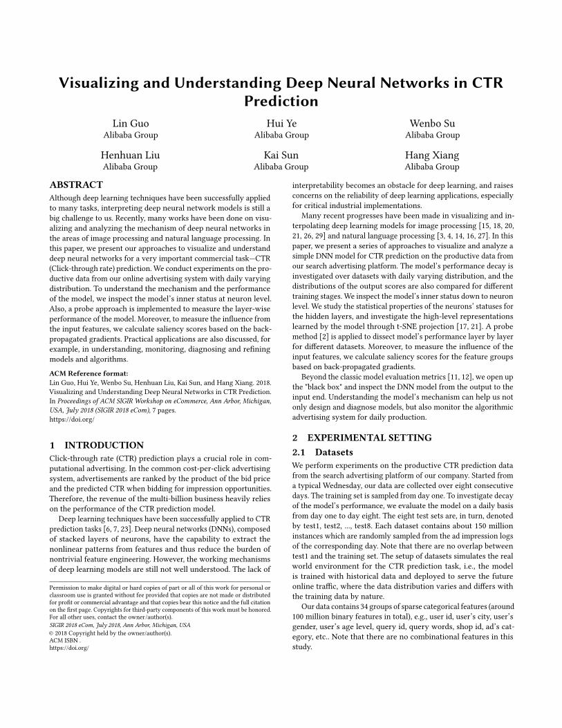
Figure 1: AUC score as a function of training step for train-ing and test sets.

To measure the performance of model, we employ AUC (areaunder curve of the receiver operating characteristic plot) as the

key metric. AUC is a widely used measure for evaluating the CTRperformance [12].

In Fig. 1, we present the evolution of the model’s AUC as afunction of the training steps for training and test sets. With thetraining going on, the train AUC keeps growing, while all the testAUCs follow a same pattern — first rises and then decreases due tooverfitting. The model generalizes best at step 210000. Comparingthe eight test AUCs for the same time step, the model’s performancedecay can be disclosed as a function of dataset. The test AUC scoredecreases monotonically from day one to day five. As expected,this is because the distribution of the test data differs with thetraining set, and the difference grows day by day. After that, AUCupswings for the last three days and surpasses day four. This is inaccordance with a characteristic of our business scene — althoughthe data varies from day to day, the users’ behaviors on our websitehave weekly periodic patterns. This non-monotonic change of AUCis evident for the regime from under-fitting to weak overfitting(before step ∼ 400000). At larger training steps, overfitting becomessevere and the model performs same bad for the last five days.

0.000

0.002

0.004

0.006

dist

ribut

ion

dens

itystep=210000

positive, trainingpositive, test1positive, test5negative, trainingnegative, test1negative, test5

0.0 0.5 1.0 1.5 2.0normalized prediction score

0.000

0.002

0.004

0.006

0.008

dist

ribut

ion

dens

ity

step=600000positive, trainingpositive, test1positive, test5negative, trainingnegative, test1negative, test5

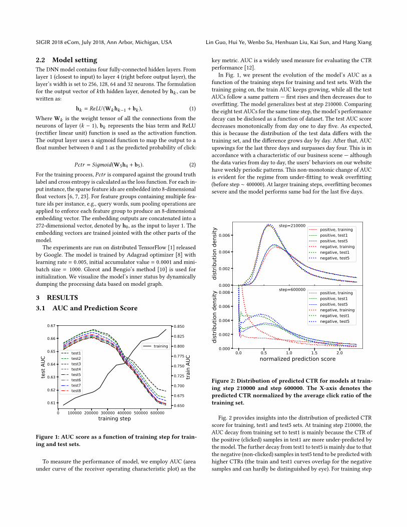
Figure 2: Distribution of predicted CTR for models at train-ing step 210000 and step 600000. The X-axis denotes thepredicted CTR normalized by the average click ratio of thetraining set.

Fig. 2 provides insights into the distribution of predicted CTRscore for training, test1 and test5 sets. At training step 210000, theAUC decay from training set to test1 is mainly because the CTR ofthe positive (clicked) samples in test1 are more under-predicted bythemodel. The further decay from test1 to test5 is mainly due to thatthe negative (non-clicked) samples in test5 tend to be predicted withhigher CTRs (the train and test1 curves overlap for the negativesamples and can hardly be distinguished by eye). For training step

Visualizing and Understanding Deep Neural Networks in CTR Prediction SIGIR 2018 eCom, July 2018, Ann Arbor, Michigan, USA

0.00

0.25step=100000 legend

trainingtest1

0.00

0.25

mea

n ou

tput step=210000

0.00

0.25 step=300000

0 2 4 6 8 10 12 14 16 18 20 22 24 26 28 30 32 34 36 38 40 42 44 46 48 50 52 54 56 58 60 62index of neuron

0.00

0.25 step=600000

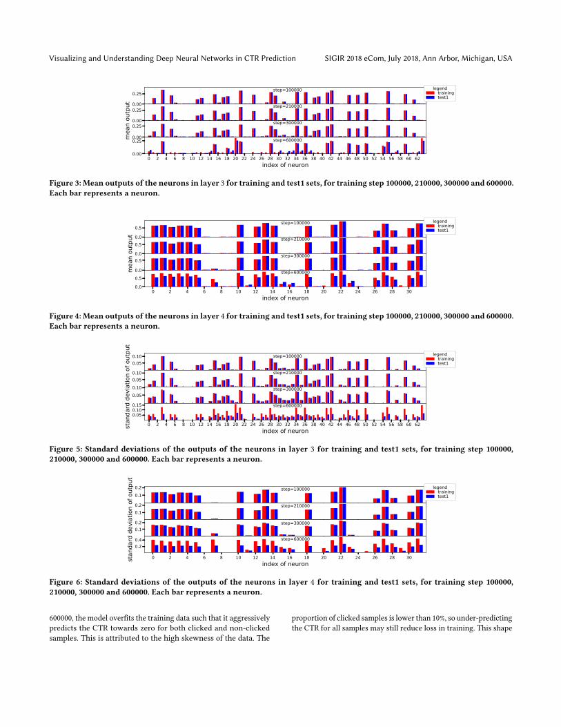
Figure 3: Mean outputs of the neurons in layer 3 for training and test1 sets, for training step 100000, 210000, 300000 and 600000.Each bar represents a neuron.

0.0

0.5step=100000 legend

trainingtest1

0.0

0.5

mea

n ou

tput step=210000

0.0

0.5step=300000

0 2 4 6 8 10 12 14 16 18 20 22 24 26 28 30index of neuron

0.00.5

step=600000

Figure 4: Mean outputs of the neurons in layer 4 for training and test1 sets, for training step 100000, 210000, 300000 and 600000.Each bar represents a neuron.

0.050.10 step=100000 legend

trainingtest1

0.050.10

stan

dard

dev

iatio

n of

out

put

step=210000

0.050.10 step=300000

0 2 4 6 8 10 12 14 16 18 20 22 24 26 28 30 32 34 36 38 40 42 44 46 48 50 52 54 56 58 60 62index of neuron

0.050.100.15 step=600000

Figure 5: Standard deviations of the outputs of the neurons in layer 3 for training and test1 sets, for training step 100000,210000, 300000 and 600000. Each bar represents a neuron.

0.10.2 step=100000 legend

trainingtest1

0.10.2

stan

dard

dev

iatio

n of

out

put

step=210000

0.10.2 step=300000

0 2 4 6 8 10 12 14 16 18 20 22 24 26 28 30index of neuron

0.20.4 step=600000

Figure 6: Standard deviations of the outputs of the neurons in layer 4 for training and test1 sets, for training step 100000,210000, 300000 and 600000. Each bar represents a neuron.

600000, the model overfits the training data such that it aggressivelypredicts the CTR towards zero for both clicked and non-clickedsamples. This is attributed to the high skewness of the data. The

proportion of clicked samples is lower than 10%, so under-predictingthe CTR for all samples may still reduce loss in training. This shape

SIGIR 2018 eCom, July 2018, Ann Arbor, Michigan, USA Lin Guo, Hui Ye, Wenbo Su, Henhuan Liu, Kai Sun, and Hang Xiang

of distribution changes significantly as the data become different,the scores move rightwards and the distribution becomes blurred.

3.2 Neuron StatusIn this subsection, we investigate the statistics of the neurons’statuses for different training stages and datasets. These statisticalproperties depict the model’s representation of the input data, andcan help us to interpret the model’s performance and workingmechanism.

0.0300

0.0305

0.0310

aver

age

stan

dard

dev

iatio

n

step=100000

0.0310

0.0315

0.0320

0.0325step=210000

train test1 test3 test5 test8data set

0.04

0.06

0.08

0.10

step=600000

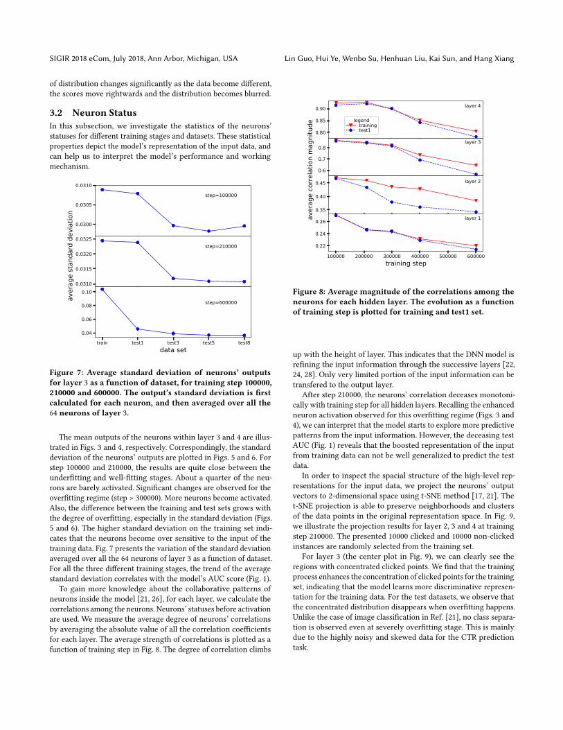
Figure 7: Average standard deviation of neurons’ outputsfor layer 3 as a function of dataset, for training step 100000,210000 and 600000. The output’s standard deviation is firstcalculated for each neuron, and then averaged over all the64 neurons of layer 3.

The mean outputs of the neurons within layer 3 and 4 are illus-trated in Figs. 3 and 4, respectively. Correspondingly, the standarddeviation of the neurons’ outputs are plotted in Figs. 5 and 6. Forstep 100000 and 210000, the results are quite close between theunderfitting and well-fitting stages. About a quarter of the neu-rons are barely activated. Significant changes are observed for theoverfitting regime (step > 300000). More neurons become activated.Also, the difference between the training and test sets grows withthe degree of overfitting, especially in the standard deviation (Figs.5 and 6). The higher standard deviation on the training set indi-cates that the neurons become over sensitive to the input of thetraining data. Fig. 7 presents the variation of the standard deviationaveraged over all the 64 neurons of layer 3 as a function of dataset.For all the three different training stages, the trend of the averagestandard deviation correlates with the model’s AUC score (Fig. 1).

To gain more knowledge about the collaborative patterns ofneurons inside the model [21, 26], for each layer, we calculate thecorrelations among the neurons. Neurons’ statuses before activationare used. We measure the average degree of neurons’ correlationsby averaging the absolute value of all the correlation coefficientsfor each layer. The average strength of correlations is plotted as afunction of training step in Fig. 8. The degree of correlation climbs

0.80

0.85

0.90

aver

age

corre

latio

n m

agni

tude

layer 4

legendtrainingtest1

0.6

0.7

0.8layer 3

0.35

0.40

0.45 layer 2

100000 200000 300000 400000 500000 600000training step

0.22

0.24

0.26 layer 1

Figure 8: Average magnitude of the correlations among theneurons for each hidden layer. The evolution as a functionof training step is plotted for training and test1 set.

up with the height of layer. This indicates that the DNN model isrefining the input information through the successive layers [22,24, 28]. Only very limited portion of the input information can betransfered to the output layer.

After step 210000, the neurons’ correlation deceases monotoni-cally with training step for all hidden layers. Recalling the enhancedneuron activation observed for this overfitting regime (Figs. 3 and4), we can interpret that the model starts to explore more predictivepatterns from the input information. However, the deceasing testAUC (Fig. 1) reveals that the boosted representation of the inputfrom training data can not be well generalized to predict the testdata.

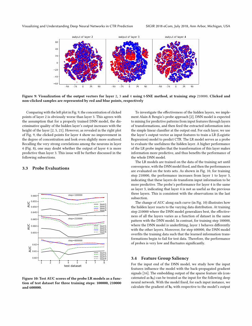
In order to inspect the spacial structure of the high-level rep-resentations for the input data, we project the neurons’ outputvectors to 2-dimensional space using t-SNE method [17, 21]. Thet-SNE projection is able to preserve neighborhoods and clustersof the data points in the original representation space. In Fig. 9,we illustrate the projection results for layer 2, 3 and 4 at trainingstep 210000. The presented 10000 clicked and 10000 non-clickedinstances are randomly selected from the training set.

For layer 3 (the center plot in Fig. 9), we can clearly see theregions with concentrated clicked points. We find that the trainingprocess enhances the concentration of clicked points for the trainingset, indicating that the model learns more discriminative represen-tation for the training data. For the test datasets, we observe thatthe concentrated distribution disappears when overfitting happens.Unlike the case of image classification in Ref. [21], no class separa-tion is observed even at severely overfitting stage. This is mainlydue to the highly noisy and skewed data for the CTR predictiontask.

Visualizing and Understanding Deep Neural Networks in CTR Prediction SIGIR 2018 eCom, July 2018, Ann Arbor, Michigan, USA

Figure 9: Visualization of the output vectors for layer 2, 3 and 4 using t-SNE method, at training step 210000. Clicked andnon-clicked samples are represented by red and blue points, respectively

Comparingwith the left plot in Fig. 9, the concentration of clickedpoints of layer 2 is obviously worse than layer 3. This agrees withthe assumption that for a properly trained DNN model, the dis-criminative quality of the hidden layer’s output increases with theheight of the layer [2, 5, 21]. However, as revealed in the right plotof Fig. 9, the clicked points for layer 4 show no improvement inthe degree of concentration and look even slightly more scattered.Recalling the very strong correlations among the neurons in layer4 (Fig. 8), one may doubt whether the output of layer 4 is morepredictive than layer 3. This issue will be further discussed in thefollowing subsections.

3.3 Probe Evaluations

0.645

0.650

0.655

0.660

AUC

step=100000

layer1layer2layer3layer4

0.655

0.660

0.665

AUC

step=210000

layer1layer2layer3layer4

1 2 3 4 5 6 7 8test dataset

0.60

0.61

0.62

AUC

step=600000

layer1layer2layer3layer4

Figure 10: Test AUC scores of the probe LRmodels as a func-tion of test dataset for three training steps: 100000, 210000and 600000.

To investigate the effectiveness of the hidden layers, we imple-ment Alain & Bengio’s probe approach [2]. DNN model is expectedto mining for predictive patterns from input features through layersof transformations, and then feed the extracted information intothe simple linear classifier at the output end. For each layer, we usethe layer’s output vector as input features to train a LR (LogisticRegression) model to predict CTR. The LR model serves as a probeto evaluate the usefulness the hidden layer. A higher performanceof the LR probe implies that the transformation of this layer makesinformation more predictive, and thus benefits the performance ofthe whole DNN model.

The LR models are trained on the data of the training set untilconvergence, with the DNNmodel fixed, and then the performancesare evaluated on the tests sets. As shown in Fig. 10, for trainingstep 210000, the performance increases from layer 1 to layer 3,indicating that these layers do transform input information to bemore predictive. The probe’s performance for layer 4 is the sameas layer 3, indicating that layer 4 is not as useful as the previousthree layers. This is consistent with the observations in the lastsubsection.

The change of AUC along each curve (in Fig. 10) illustrates howthe hidden layer reacts to the varying data distribution. At trainingstep 210000 where the DNN model generalizes best, the effective-ness of all the layers varies as a function of dataset in the samepattern with the DNN model. In contrast, for training step 100000,where the DNN model is underfitting, layer 1 behaves differentlywith the other layers. Moreover, for step 600000, the DNN modeloverfits the training data such that the learned information trans-formations begin to fail for test data. Therefore, the performanceof probes is very low and fluctuates significantly.

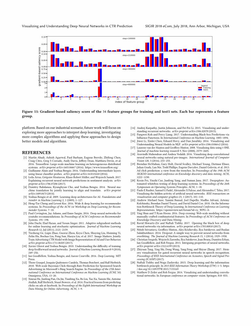
3.4 Feature Group SaliencyFor the input end of the DNN model, we study how the inputfeatures influence the model with the back-propagated gradientsignals [16]. The embedding output of the sparse feature ids (con-catenated as h0) can be treated as the input for the following deepneural network. With the model fixed, for each input instance, wecalculate the gradient of h0 with respective to the model’s output

SIGIR 2018 eCom, July 2018, Ann Arbor, Michigan, USA Lin Guo, Hui Ye, Wenbo Su, Henhuan Liu, Kai Sun, and Hang Xiang

Pctr :

g0 = ∇h0Pctr . (3)

The magnitude of each element of the gradient vector g0 quanti-fies the sensitivity of the model’s output to the change in the par-ticular embedding element. It describe how much a small changein a particular embedding value could affect the final output Pctr .Given a dataset, we calculate the saliency score for each featuregroup by averaging the mean absolute value of the corresponding 8gradient elements in g0 over the whole dataset. This saliency scoreprovides us with an average measure of the model’s sensitivity toeach feature group for the given dataset.

We illustrate the saliency scores in Fig. 11. Overall, the modelis becoming increasingly sensitive to all the feature groups duringtraining. In the overfitting regime, the score of feature group 10 risesup dramatically and becomes much higher than the other featuregroups. This feature group is composed of user ids, in which thenumber of ids is larger than any other feature group by at leasttwo orders of magnitude [9]. For this training stage, the model istrained to memorize the vast amount of information from user idsthat is not generalizable, and thus significantly deteriorates theperformance on test datasets.

4 DISCUSSION4.1 Role of Layer 4The results about layer 4 raise a question about the necessity toinclude this layer in the model. To answer this question, we modifythe neural network and investigate the impact on performance ofthe retrained models. We modify layer 4 by reducing or increas-ing its width by a factor of two, or even remove layer 4 from themodel. It turns out that these modifications do not affect the mod-els’ performance (highest test AUCs) for the different test dataset.Although not harmful, there is no benefit to include layer 4 in theDNN model.

4.2 RegularizationAnalysis in the previous section reveals that the model become oversensitive to the input when overfitting. Also, the high correlationsamong neurons for layer 3 and 4 (Fig. 8) imply that there might besevere co-adaptations [25]. One may hope to use regularizationsto control overfitting and obtain better performance on test data.We have tried L1 and L2 regularization [11], and dropout [25], for avariety of hyper-parameters. However, no improvement is obtained.In future, more work needs to be conducted on improving model’sgeneralization power.

4.3 Feature TreatmentSubsection 3.4 discloses the problem that the model is greatly sen-sitive to the feature group of user ids when overfitting. Other thanregularization, it is also possible to improve the models’ general-ization power by optimizing the input features. User id is a highlygranular feature group. Inputting it directly to the embedding-baseddeep neural network may not be the optimal choice. Following theidea of Wide&Deep [6], we remove user id from the embeddinglayer. The bias of each user id is represented by a float numberbuser and added immediately into the output layer:

Pctr = Siдmoid(W5h4 + b5 + buser ). (4)

This bias is trained jointly with the other parts of the model. Wefind this approach can improve AUC on the test datasets by about0.1%.

5 APPLICATIONSWith the visualization and analysis techniques presented above, wediscuss some of the practical applications in this section.• The distribution of the predicted CTR score is very important forreal-time bidding auctions. Understanding the score distributioncan help us to design better calibration methods [13, 19]. Also,score distribution can help to find outliers or bad-fitted samples,which can in turn be used to improve the model.

• Inspections of model’s inner status and gradient signals openup the "black box" of the DNN model, helping us to understandthe mechanism of the model and the influence of features. Theseapproaches can be used to diagnose the model, like (but notlimited to) underfitting/overfitting, gradient vanishing/explosion,ineffective model structure, etc.. A deep understanding of themodel’s mechanism can help us to design better model structure,training algorithm and features.

• For online advertisting, it is of great importance to monitor themodel’s online performance and the health of data pipeline. Feed-ing the model with problematic data can cause disaster. However,it is very difficult to describe and monitor the distribution of theextremely sparse and high-dimensional data. Moreover, monitor-ing the model’s online performance may not be sufficient. Themodel predicts CTR for hundreds of candidate ads for each biding,while only very few ads can win the bidding and get feedbackfrom impression. The classic performance metrics are mainlybased on those feedbacks, and thus can only cover a limitedportion of biased data.The DNN model, by nature, transforms the sparse input datainto dense numerical representations. Therefore, the statistics ofneurons’ output and the gradient signals can be implemented asa new kind of metrics to monitor the distribution of the inputdata. Note that no feedback labels are needed to calculate thesequantities. For example, as illustrated in Fig. 7, the average stan-dard deviation for layer 3’s output changes with the naturallyvarying distribution of input data. Problematic input data cancause more significant change in the statistics.

6 CONCLUSIONIn this work, we visualize and analyze a simple DNNmodel for CTRprediction down to neuron level. Model training and evaluationsare performed over a series of datasets. The model is inspected fromthe output to the input end. The statuses of neurons are studiedusing a variety of methods. Gradients of the feature embeddingsare used to create a salience map to describe the influence of thefeature groups. The analysis provides insightful knowledges of themodel’s mechanism, helping us to monitor, diagnose and refine themodel.

Currently, we are applying these approaches to build a model-based evaluation and monitoring system for our online advertising

Visualizing and Understanding Deep Neural Networks in CTR Prediction SIGIR 2018 eCom, July 2018, Ann Arbor, Michigan, USA

0.00

0.05

0.10 step=100000

0.00

0.05

0.10 step=210000

0.00

0.25

0.50

0.75

grad

ient

-bas

ed sa

lienc

y sc

ore

step=300000

0 2 4 6 8 10 12 14 16 18 20 22 24 26 28 30 32index of feature group

0

1

2

3 step=600000 legendtrainingtest1

Figure 11: Gradient-based saliency score of the 34 feature groups for training and test1 sets. Each bar represents a featuregroup.

platform. Based on our industrial scenario, future workwill focus onexploring more approaches to interpret deep learning, investigatingmore complex algorithms and applying these approaches to designbetter models and algorithms.

REFERENCES[1] Martín Abadi, Ashish Agarwal, Paul Barham, Eugene Brevdo, Zhifeng Chen,

Craig Citro, Greg S Corrado, Andy Davis, Jeffrey Dean, Matthieu Devin, et al.2016. Tensorflow: Large-scale machine learning on heterogeneous distributedsystems. arXiv preprint arXiv:1603.04467 (2016). https://www.tensorflow.org/

[2] Guillaume Alain and Yoshua Bengio. 2016. Understanding intermediate layersusing linear classifier probes. arXiv preprint arXiv:1610.01644 (2016).

[3] Leila Arras, Grégoire Montavon, Klaus-Robert Müller, and Wojciech Samek. 2017.Explaining recurrent neural network predictions in sentiment analysis. arXivpreprint arXiv:1706.07206 (2017).

[4] Dzmitry Bahdanau, Kyunghyun Cho, and Yoshua Bengio. 2014. Neural ma-chine translation by jointly learning to align and translate. arXiv preprintarXiv:1409.0473 (2014).

[5] Yoshua Bengio et al. 2009. Learning deep architectures for AI. Foundations andtrends® in Machine Learning 2, 1 (2009), 1–127.

[6] Heng-Tze Cheng and Levent Koc. 2016. Wide & deep learning for recommendersystems. In Proceedings of the ACM 1st Workshop on Deep Learning for Recom-mender Systems. 7–10.

[7] Paul Covington, Jay Adams, and Emre Sargin. 2016. Deep neural networks foryoutube recommendations. In Proceedings of ACM Conference on RecommenderSystems. 191–198.

[8] John Duchi, Elad Hazan, and Yoram Singer. 2011. Adaptive subgradient methodsfor online learning and stochastic optimization. Journal of Machine LearningResearch 12, Jul (2011), 2121–2159.

[9] Tiezheng Ge, Liqin Zhao, Guorui Zhou, Keyu Chen, Shuying Liu, Huiming Yi,Zelin Hu, Bochao Liu, Peng Sun, Haoyu Liu, et al. 2017. Image Matters: JointlyTrain Advertising CTRModel with Image Representation of Ad and User Behavior.arXiv preprint arXiv:1711.06505 (2017).

[10] Xavier Glorot and Yoshua Bengio. 2010. Understanding the difficulty of trainingdeep feedforward neural networks. Journal of Machine Learning Research 9 (2010),249–256.

[11] Ian Goodfellow, Yoshua Bengio, and Aaron Courville. 2016. Deep Learning. MITPress.

[12] Thore Graepel, Joaquin Quiñonero Candela, Thomas Borchert, and Ralf Herbrich.2010. Web-scale Bayesian Click-through Rate Prediction for Sponsored SearchAdvertising in Microsoft’s Bing Search Engine. In Proceedings of the 27th Inter-national Conference on International Conference on Machine Learning (ICML’10).Omnipress, USA, 13–20.

[13] Xinran He, Junfeng Pan, Ou Jin, Tianbing Xu, Bo Liu, Tao Xu, Yanxin Shi, AntoineAtallah, Ralf Herbrich, Stuart Bowers, et al. 2014. Practical lessons from predictingclicks on ads at facebook. In Proceedings of the Eighth International Workshop onData Mining for Online Advertising. ACM, 1–9.

[14] Andrej Karpathy, Justin Johnson, and Fei-Fei Li. 2015. Visualizing and under-standing recurrent networks. arXiv preprint arXiv:1506.02078 (2015).

[15] Pangwei Koh and Percy Liang. 2017. Understanding Black-box Predictions viaInfluence Functions. In International Conference on Machine Learning. 1885–1894.

[16] Jiwei Li, Xinlei Chen, Eduard Hovy, and Dan Jurafsky. 2016. Visualizing andUnderstanding Neural Models in NLP. arXiv preprint arXiv:1506.01066v2 (2016).

[17] Laurens van der Maaten and Geoffrey Hinton. 2008. Visualizing data using t-SNE.Journal of machine learning research 9, Nov (2008), 2579–2605.

[18] Aravindh Mahendran and Andrea Vedaldi. 2016. Visualizing deep convolutionalneural networks using natural pre-images. International Journal of ComputerVision 120, 3 (2016), 233–255.

[19] Brendan McMahan, Gary Holt, David Sculley, Michael Young, Dietmar Ebner,Julian Grady, Lan Nie, Todd Phillips, Eugene Davydov, Daniel Golovin, et al. 2013.Ad click prediction: a view from the trenches. In Proceedings of the 19th ACMSIGKDD international conference on Knowledge discovery and data mining. ACM,1222–1230.

[20] Kexin Pei, Yinzhi Cao, Junfeng Yang, and Suman Jana. 2017. Deepxplore: Au-tomated whitebox testing of deep learning systems. In Proceedings of the 26thSymposium on Operating Systems Principles. ACM, 1–18.

[21] Paulo E Rauber, Samuel G Fadel, Alexandre X Falcao, and Alexandru C Telea. 2017.Visualizing the hidden activity of artificial neural networks. IEEE transactions onvisualization and computer graphics 23, 1 (2017), 101–110.

[22] Andrew Michael Saxe, Yamini Bansal, Joel Dapello, Madhu Advani, ArtemyKolchinsky, Brendan Daniel Tracey, and David Daniel Cox. 2018. On the Informa-tion Bottleneck Theory of Deep Learning. In International Conference on LearningRepresentations. https://openreview.net/forum?id=ry_WPG-A-

[23] Ying Shan and T Ryan Hoens. 2016. Deep crossing: Web-scale modeling withoutmanually crafted combinatorial features. In Proceedings of ACM Conference onKnowledge Discovery and Data Mining.

[24] Ravid Shwartz-Ziv and Naftali Tishby. 2017. Opening the black box of deepneural networks via information. arXiv preprint arXiv:1703.00810 (2017).

[25] Nitish Srivastava, Geoffrey Hinton, Alex Krizhevsky, Ilya Sutskever, and RuslanSalakhutdinov. 2014. Dropout: A simple way to prevent neural networks fromoverfitting. The Journal of Machine Learning Research 15, 1 (2014), 1929–1958.

[26] Christian Szegedy,Wojciech Zaremba, Ilya Sutskever, Joan Bruna, Dumitru Erhan,Ian Goodfellow, and Rob Fergus. 2013. Intriguing properties of neural networks.arXiv preprint arXiv:1312.6199 (2013).

[27] Zhiyuan Tang, Ying Shi, Dong Wang, Yang Feng, and Shiyue Zhang. 2017. Mem-ory visualization for gated recurrent neural networks in speech recognition.Proceedings of IEEE International Conference on Acoustics, Speech and Signal Pro-cessing (ICASSP) (2017).

[28] Naftali Tishby and Noga Zaslavsky. 2015. Deep learning and the informationbottleneck principle. In 2015 IEEE Information Theory Workshop (ITW). 1–5. https://doi.org/10.1109/ITW.2015.7133169

[29] Matthew D Zeiler and Rob Fergus. 2014. Visualizing and understanding convolu-tional networks. In European conference on computer vision. Springer, 818–833.