ijssbt.comijssbt.com/downloads/ijssbt vol-2 no. 2 may 14.pdf · 3d vision 3d tv biometrics...
TRANSCRIPT


PRATIBHA: INTERNATIONAL JOURNAL OF SCIENCE,
SPIRITUALITY, BUSINESS AND TECHNOLOGY (IJSSBT)
Pratibha: International Journal of Science, Spirituality, Business and Technology
(IJSSBT) is a research journal published by Shram Sadhana Bombay Trust‘s, COLLEGE Of
ENGINEERING & TECHNOLOGY, Bambhori, Jalgaon, MAHARASHTRA STATE, INDIA. College was
founded by FORMER PRESIDENT, GOVT. OF INDIA, Honorable Excellency Sau.
PRATIBHA DEVI SINGH PATIL.
College is awarded as Best Engineering College of Maharashtra State by Engineering Education Foundation, Pune in year 2008-09.
The College has ten full-fledged departments. The Under Graduate programs in 7
courses are accredited by National Board of Accreditation, All India Council for
Technical Education, New Delhi for 5 years with effect from 19/07/2008 vide letter
number NBA/ACCR-414/2004. QMS of the College conforms to ISO 9001:2008 and is
certified by JAAZ under the certificate number: 1017-QMS-0117.The college has been
included in the list of colleges prepared under Section 2(f) of the UGC Act, 1956 vide
letter number F 8-40/2008 (CPP-I) dated May, 2008 and 12(B) vide letter number F. No.
8-40/2008(CPP-I/C) dated September 2010.UG courses permanently affiliated to North
Maharashtra University are: Civil Engineering, Chemical Engineering, Computer
Engineering, Electronics and Telecommunication Engineering, Electrical Engineering,
Mechanical Engineering, Information Technology. Two years Post Graduate courses are
Mechanical Engineering (Machine Design), Civil Engineering (Environmental
Engineering), Computer Engineering (Computer Science and Engineering), Electronics,
Telecommunication(Digital Electronics) and Electrical Engineering (Electrical power
systems). Civil Engineering Department, Mechanical, Biotechnology and Chemical
Engineering Department laboratories are registered for Ph.D. Programs. Spread over 25
Acres, the campus of the college is beautifully located on the bank of river Girna.
The International Journal of Science, Spirituality, Business and Technology
(IJSSBT) is an excellent, intellectual, peer reviewed journal that takes scholarly approach
in creating, developing, integrating, sharing and applying knowledge about all the fields
of study in Engineering, Spirituality, Management and Science for the benefit of
humanity and the profession.
The audience includes researchers, managers, engineers, curriculum designers
administrators as well as developers.

AIM AND SCOPE
Our philosophy is to map new frontiers in emerging and developing technology areas in research,
industry and governance, and to link with centers of excellence worldwide to provide
authoritative coverage and references in focused and specialised fields. The journal presents its
readers with broad coverage across all branches of Engineering, Management, Spirituality and
Science of the latest development and their applications.
All technical, research papers and research results submitted to IJSSBT should be original in
nature. Contributions should be written for one of the following categories:
1. Original research
2. Research Review / Systematic Literature Review
3. Short Articles on ongoing research
4. Preliminary Findings
5. Technical Reports / Notes
IJSSBT publishes on the following topics but NOT LIMITED TO:
SCIENCES
Computational and industrial
mathematics and statistics, and other
related areas of mathematical sciences
Approximation theory
Computation
Systems control
Differential equations and dynamical
systems
Financial math
Fluid mechanics and solid mechanics
Functional calculus and applications
Linear and nonlinear waves
Numerical algorithms
Numerical analysis
Operations research
Optimization
Probability and stochastic processes
Simulation
Statistics
Wavelets and wavelet transforms
Inverse problems
Artificial intelligence
Neural processing
Nuclear and particle physics
Geophysics
Physics in medicine and biology
Plasma physics
Semiconductor science and
technology
Wireless and optical communications
Materials science
Energy and fuels
Environmental science and
technology
Combinatorial chemistry
Natural products
Molecular therapeutics
Geochemistry
Cement and concrete research,
Metallurgy
Crystallography and
Computer-aided materials design
COMPUTER ENGINEERING AND INFORMATION TECHNOLOGY
Information Systems e-Commerce
Intelligent Systems
Information Technology
e-Government
Language and Search Engine Design
Data Mining and Web Mining
Cloud Computing
Distributed Computing
Telecommunication Systems

Artificial Intelligence
Virtual Business and Enterprise
Computer Systems
Computer Networks
Database Systems and Theory
Knowledge Management
Computational Intelligence
Simulation and Modeling
Scientific Computing and HPC
Embedded Systems
Control Systems
ELECTRONICS AND TELECOMMUNICATION ENGINEERING
3D Vision
3D TV
Biometrics
Graph-based Methods
Image and video indexing and
database retrieval
Image and video processing
Image-based modeling
Kernel methods
Model-based vision approaches
Motion Analysis
Non-photorealistic animation and
modeling
Object recognition
Performance evaluation
Segmentation and grouping
Shape representation and analysis
Structural pattern recognition
Computer Graphics Systems and
Hardware
Rendering Techniques and Global
Illumination
Real-Time Rendering
Fast Algorithms
Fast Fourier Transforms
Digital Signal Processing
Wavelet Transforms
Mobile Signal Processing
Statistical Signal Processing
Optical Signal Processing
Data Mining Techniques
Motion Detection
Content-based Image retrieval
Video Signal Processing
Watermarking
Signal Identification
Detection and Estimation of Signal
Parameters
Nonlinear Signals and Systems
Signal Reconstruction
Time-Frequency Signal Analysis
Filter Design and Structures
Spectral Analysis
Adaptive and Clustering Algorithms
Fast Fourier Transforms
Virtual, Augmented and Mixed
Reality
Geometric Computing and Solid
Modeling
Game Design and Engine
Development
3D Reconstruction
GPU Programming
Graphics and Multimedia
Image Processing
Interactive Environments
Software and Web accessibility
Graphics & Perception
Computational Photography
Pattern recognition and analysis
Medical image processing
Visualization
Image coding and compression
Face Recognition
Image segmentation
Radar Image Processing
Sonar Image Processing
Signal Identification
Super-resolution imaging
Signal Reconstruction
Filter Design
Adaptive Filters
Multi-channel Filtering
Noise Control
Control theory and practice
CIVIL ENGINEERING
Geotechnical
Structures
Transportation
Environmental Engineering
Earthquakes
Water Resources
Hydraulic and Hydraulic Structures

Construction Management, and
Material
Structural mechanics
Soil mechanics and Foundation
Engineering
Coastal engineering and River
engineering
Ocean Engineering
Fluid-solid-structure interactions,
offshore engineering and marine
structures
Constructional management and other
civil engineering relevant areas
Surveying
Transportation Engineering
CHEMICAL ENGINEERING
Organic Chemistry
Inorganic Chemistry
Physical Chemistry
Analytical Chemistry
Biological Chemistry
Industrial Chemistry
Agricultural & Soil Chemistry
Petroleum Chemistry
Polymers Chemistry
Nanotechnology
Green Chemistry
Forensic
Photochemistry
Computational
Chemical Physics
Chemical Engineering
Wastewater treatment and engineering
Biosorption
Chemisorptions
Heavy metal remediation
Phytoremediation
Novel treatment processes for
wastewaters
Land reclamation methods
Solid waste treatment
Anaerobic digestion
Gasification
Landfill issues
Leachate treatment and gasification
Water and Wastewater Minimization
Mass integration
Emission Targeting
Pollution Control
Safety and Loss Prevention
Conceptual Design
Mathematical Approach
Pinch Technology
Energy Audit
Production Technical Knowledge
Process Design
Heat Transfer
Chemical Reaction Engineering
Modeling and simulation
Process Equipment Design
ELECTRICAL ENGINEERING
Power Engineering
Electrical Machines
Instrumentation and control
Electric Power Generation
Transmission and Distribution
Power Electronics
Power Quality and Economic
Renewable Energy
Electric Traction, Electromagnetic
Compatibility and Electrical
Engineering Materials
High Voltage Insulation Technologies
High Voltage Apparatuses
Lightning Detection and Protection
Power System Analysis, SCADA and
Electrical Measurements
MECHANICAL ENGINEERING
Fluid mechanics
Heat transfer
Solid mechanics
Refrigeration and air conditioning
Renewable energy technology
Materials engineering
Composite materials
Marine engineering
Petroleum and mineral resources
engineering
Textile engineering
Leather technology

Industrial engineering
Operational research
Manufacturing processes
Machine design
Quality control
Mechanical maintenance
Tribology
MANAGEMENT
Accounting and Finance
Marketing
Operations Management
Human resource management
Management Strategy
Information technology
Business Economics
Public Sector management
Organizational behavior
Research methods
SPIRITUALITY
Relevance of Science and Spirituality
in decision and Policy making
Rigors in Scientific Research and
Insights from Spiritual wisdom
Dividends from Scientific research
and Spiritual Temper
Spiritual Wisdom in disaster
management
Techno-Spiritual aspects of
development
BIO-TECHNOLOGY
Molecular biology and the chemistry
of biological process to aquatic and
earth environmental aspects as well as
computational applications
Policy and ethical issues directly
related to Biotechnology
Molecular biology
Genetic engineering
Microbial biotechnology
Plant biotechnology
Animal biotechnology
Marine biotechnology
Environmental biotechnology
Biological processes
Industrial applications
Bioinformatics
Biochemistry of the living cell
Bioenergetics

IJSSBT prides itself in ensuring the high quality and professional standards.
All submitted papers are to be peer-reviewed for ensuring their qualities.
Frequency : Two issues per year
Page charges : There are no page charges to individuals or institutions.
ISSN : 2277-7261 (Print version) and 2278-3857 (on-line)
Subject Category : Science, Engineering, Business and Spirituality
Published by : Shram Sadhana Bombay Trust’s, College of Engineering and
Technology, Bambhori, Jalgaon, M.S., India
REQUIREMENTS FOR MANUSCRIPT PREPARATION
The following information provides guidance in preparing manuscript for IJSSBT.
Papers are accepted only in English.
Papers of original research, research review/systematic literature review, short articles on
ongoing research, preliminary findings, and technical reports/notes should not exceed 15
typeset, printed pages.
Abstracts of 150-200 words are required for all papers submitted.
Each paper should have three to six keywords. Section headings should be concise and
numbered sequentially as per the following format.
All the authors (maximum three authors) of a paper should include their full names,
affiliations, postal address, telephone and fax numbers and email address on the cover
page of the manuscript as per following format. One author should be identified as the
CorrespondingAuthor.
Biographical notes on contributors are not required for this journal.
For all manuscripts non-discriminatory language is mandatory. Sexist or racist terms
should not be used.
Authors must adhere to SIunits . Units are not italicized.
The title of the paper should be concise and definitive (with key words appropriate for
retrieval purposes).
Manuscript Format
Document : The Manuscript should be prepared in English language by using MS
Word (.doc format). An IJSSBT paper should not exceed 15 typeset,
printed pages including references, figures and abstract etc.
Paper : Use A4 type paper page (8.27″x 11.69″).
Paper format: two columns with equal width and spacing of 0.25″.
Margins : Leave margins of article 1.3" at the left and for top, bottom, and right
sides 1″.
Font Size and Style: 10 Point Times new roman, and typed in single space, Justified.
Title Page :

Title of the paper should be in bold face, Title case: font size 16, Times New Roman,
centered.
Name of the authors in normal face, Title case: font size 11 italic, Times New Roman.
Addresses and affiliations of all authors: normal face, title case font size 10, Times New
Roman.
Email address: normal face, lower case font size 10, Times New Roman.
Abstract (Font size 10, bold face) Abstract should be in brief and structured. The abstract should tell the context, basic procedure,
main findings and principle conclusions. It should emphasize new aspect of study or research.
Avoid abbreviation, diagram and references in abstract. It should be single spaced and should not
exceed more than 200 words.
Keywords:(Font size 10, bold face, italic)
I. INTRODUCTION(Font size 10, bold face)
Provide background, nature of the problem and its significance. The research objective is often
more sharply focused when stated as a question. Both the main and secondary objectives should
be clear. It should not include data or conclusions from the work being reported.
All Main Heading with Roman numbers(Font size 10, bold face)
With Subheading of (Font size 10, bold face, Title Case with A, B, C…..Numbering)
Picture / Figure : Pictures and figures should be appropriately included in the
main text, e.g. Fig No. 1 (Font size 9).
Table format : Font: Times New Roman, font size: 10
e.g. Table No. 1 (Font size 9)
References (font size 8, Times New Roman)
References should be arranged alphabetically with numbering. References must be complete and
properly formatted. Authors should prepare the references according to the following guidelines.
For a book:
References must consist of last name and initials of author(s), year of publication, title of book
(italicized), publisher‘s name, and total pages.
[1] Name and initial of the Author, ―Topic Name‖, title of the book, Publisher name, Page
numbers, Year of publication.
For a chapter in a book:
References must consist of last name and initials of author(s), year of publication, title of chapter,
title of book (italicized), publisher‘s name, and inclusive pages for the chapter.
[1] Name and initial of Author, ―Title of chapter‖, title of the book, Publisher name, total pages
of chapter, year of publication.

For a Journal article: Journals must consist of last name and initials of author(s), year of publication of journal, title of
paper, title of journal (italicized),volume of journal, page numbers (beginning of article - end of
article).
[1] Name and initial of the Author, ―topic name‖, title of journal, volume & issue of the journal;
Page numbers of article, year of publication.
Conference Proceedings: References must consist of last name and initials of author(s), year of publication, title of paper,
indication of the publication as proceedings, or extended abstracts volume; name of the
conference (italicized or underlined), city and state and Country where conference was held,
conference sponsor‘s name, and pages of the paper.
[1] Name and initial of the Author, title of the paper, Proceedings, name of the conference, City,
State, country, page numbers of the paper, Year of publication.
The title of the journal is italicized and font size 8, Times New Roman.
Final Submission:
Each final full text paper (.doc, .pdf) along with corresponding signed copyright transfer form
should be submitted by email -
[email protected], [email protected]
Website: www.ijssbt.org/com

S.S.B.T.’S COLLEGE OF ENGINEERING & TECHNOLOGY, BAMBHORI,
JALGAON
GOVERNING BODY
Dr. D. R. Shekhawat Chairman
Shri Rajendrasingh D. Shekhawat Managing Trustee & Member
Shri V. R. Phadnis Member
Shri Jayesh Rathore Member
Mrs. Jyoti Rathore Member
Dr. R. H. Gupta Member
Arch. Shashikant R. Kulkarni Member
Dr. K.S. Wani Principal & Ex-Officio Member Secretary
Shri S. P. Shekhawat Asso. Prof. & Member
Shri Shantanu Vasishtha Asstt. Prof. & Member
LOCAL MANAGEMENT COMMITTEE
Dr. D. R. Shekhawat Chairman
Shri Rajendrasingh D. Shekhawat Managing Trustee & Member
Shri V. R. Phadnis Member
Dr. R. H. Gupta Member
Arch. Shashikant R. Kulkarni Member
Dr. K.S. Wani Principal & Ex-Officio Member Secretary
Shri S. P. Shekhawat
(Representative of Teaching Staff)
Asso. Prof. & Member
Shri Shantanu Vasishtha
(Representative of Teaching Staff)
Asstt. Prof. & Member
Shri S. R. Girase
(Representative of Non-Teaching Staff)
Member

EDITOR(s)-IN-CHIEF
Prof. Dr. K. S. WANI,
M. Tech. (Chem. Tech.), D.B.M., Ph. D.
LMISTE, LMAFST, MOTAI, LMBRSI
Principal,
S.S.B.T.‘s College of Engineering and Technology,
P.B. 94, Bambhori,
Jalgaon-425001 Maharashtra, India
Mobile No. +919422787643
Phone No. (0257) 2258393,
Fax No. (0257) 2258392,
Email id: [email protected]
Prof. Dr. DHEERAJ SHESHRAO DESHMUKH
D,M.E., B.E.(Mechanical), M.Tech. (Heat power engineering)
Ph.D. (Mechanical Engineering)
LMISTE,
Professor and Head,
Department of Mechanical Engineering,
S.S.B.T.‘s, College of Engineering and Technology,
P.B. 94, Bambhori,
Jalgaon-425001, Maharashtra State, India
Mobile No. +91 9822418116
Phone No. (0257) 2258393,
Fax No. (0257) 2258392.
Email id : [email protected]
Web Address : www.ijssbt.org/com
EDITORIAL BOARD
PROF. SUBRAMANIAM GANESAN Director, Real Time & DSP Lab.,
Electrical and Computer Engineering Department,
Oakland University, Rochester, MI 48309, USA.
IEEE Distinguished Visiting Speaker (2005-2009) and Coordinator.
IEEE SEM CS chapter Chair, Region 4 and CS Society Board member
SAE, ASEE, ACM member
PROF. ALOK VERMA
Old Dominion University
Norfolk
Virginia, USA
PROF. EVANGELINE GUTIERREZ
Programme Manager, Global Science and Technology Forum Pvt. Ltd
10 Anson Road, Singapore

Dr. G.P. PATIL
Distinguish Professor of Mathematics Statistics
Director, Center for Statistical Ecology and Environmental Statistics
Editor-in-Chief, Environmental and Ecological Statistics
Department of Statistics
The Pennsylvania State University, USA
Dr. ABAD A. SHAH
Professor, Department of Computer Science & Engineering
University of Engineering and Technology
G. T. Road Lahore, Pakistan
Dr. ANSHUMAN TRIPATHI
Ph.D.
Principal Engineer VESTAF, SINGAPORE
Dr. MUHAMMAD MASROOR ALI
Professor, Department of Computer Science and Engineering
Bangladesh University of Engineering and Technology
Dhaka-1000, Bangladesh [email protected]
Dr. RAMESH CHANDRA GOEL
Former Director General
Deharadun Institute of Technology
Deharadun,Uttarakhad, India
Dr. DINESH CHANDRA
Ph. D.
Professor
Department of Electrical Engineering
Motilal Nehru National Institute of Technology
Allahabad-U.P., India
Dr. BHARTI DWIVEDI
Ph. D.
Professor
Department of Electrical Engineering
Government Institute of Engineering & Technology
Luknow, India
Dr. L. A. Patil
Ph. D.
Professor & Head
Dept of Physics
Pratap College Amalner
Jalgaon, India

Dr. M. QASIM RAFIQ
Ph. D. (Computer Engineering)
Professor
Senior Member IEEE (USA)
FIETE, FIE, LMCSI
Department of Computer Engineering
Z.H. College of Engineering & Technology
Aligarh Muslim University (A.M.U.)Aligarh, India
Dr. RAZAULLHA KHAN
Ph. D. (Civil Engineering)
Professor
Department of Civil Engineering
Z.H. College of Engineering & Technology
Aligarh Muslim University (A.M.U.)
Aligarh, India
Dr. K. HANS RAJ
Professor
Department of Mechanical Engineering
Faculty of Engineering
Dayalbagh Educational Institute, Dayalbagh
AGRA-India
Dr. DURGESH KUMAR MISHRA Professor and Head (CSE), Dean (R&D)
Acropolis Institute of Technology and Research, Indore, MP, India
Chairman, IEEE Computer Society, Bombay Chapter
Chairman IEEE MP Subsection
Chairman CSI Indore Chapter
Dr. SUDHIR CHINCHOLKAR
Ph.D. Microbiology
Professor & Head (Microbiology)
N.M.U. University, Jalgaon, India
Dr. M. A. LOKHANDE
Ph. D.
Professor and Head
Department of Commerce
Member Indian Commerce Association
Dr. Babasaheb Ambedkar Marathwada University, Aurangabad, India
Dr. K. K. SHUKLA
Ph.D.
Professor
Department of Civil Engineering
Motilal Nehru National Institute of Technology
Allahabad- U.P., India

Dr. RAHUL CAPRIHAN
Ph.D.
Professor
Department of Mechanical Engineering
Faculty of Engineering
Dayalbagh Educational Institute
Dayalbagh, Agra, India
Dr.SATISH KUMAR
Ph. D.
Professor
Department of Electrical Engineering
Faculty of Engineering
Dayalbagh Educational Institute
Dayalbagh, Agra, India
Dr. VED VYAS J. DWIVEDI Professor (Electronics and Communication Engineering)
Director
Noble Group of Institutions, Junagadh, Gujarat, India
*Editor-in-Chief*
*International Journal on Science and Technology*
Dr. RAM PAL SINGH
Ph.D.
Professor
Department of Civil Engineering
Motilal Nehru National Institute of Technology
Allahabad- India
Dr. ANURAG TRIPATHI
Ph.D.
Professor
Department of Electrical Engineering
Government Institute of Engineering & Technology
Luknow, India
Dr. (Mrs.) ARUNIMA DE
Ph.D.
Professor
Department of Electrical Engineering
Government Institute of Engineering & Technology
Luknow, India
Dr. A.P. DONGRE
Ph. D.
Department of Management Studies
North Maharashtra University, Jalgaon India

Dr. V. VENKATACHALAM
Principal, The Kavery Engineering College,
Mecheri. Salem District.
Dr. T. RAVICHANDRAN Research Supervisor,
Professor & Principal
Hindustan Institute of Technology
Coimbatore, Tamil Nadu, India
Dr. BHUSHAN TRIVEDI
Professor & Director, GLS-MCA, Ahmedabad.
Dr. NEERAJ BHARGAVA
HoD, Department of Computer Science,
MDS University, Ajmer.
Dr. CRISTINA NITA-ROTARU
Purdue University
Dr. RUPA HIREMATH
Director, IIPM, Pune
Dr. A. R. PATEL
HoD, Department of Computer Science,
H. North Gujarat University, Patan. Gujarat
Dr. PRIYANKA SHARMA
Professor, ISTAR, VV Nagar,
Gujarat.
Dr. V.P.ARUNACHALAM
Principal
SNS College of Technology
Sathy Main Road,
Coimbatore - 35.
Dr. B. S. AGRAWAL Gujarat
Dr. SATYEN PARIKH
Professor, Dept of Comp Sci.
Ganpat University, Mehsana. Gujarat.
Dr. P. V. VIRAPARIA
VVNagar, Gujarat.

Dr. ARUMUGANATHAN
Professor, Department of Mathematics and Computer Applications
PSG College of Technology, Coimbatore-641 004
Tamilnadu, INDIA.
Dr. H. B. BHADKA
Director (I/c)
C. U. Shah College of Master of Computer Application
Campus of C. U. Shah College of Engineering & Technology
Surendranagar-Ahmedabad
Dr. MOHAMMED MUSSADIQ
Ph. D.
Professor & Head, Department of Microbiology,
Shri Shivaji College of Arts, Commerce & Science, Akola.
Dr. ZIA-ULHASAN KHAN
Ph. D.
Professor & Head, Department of Biochemistry,
Shri Shivaji College of Arts, Commerce & Science, Akola.
Dr. SHAILENDRA KUMAR MITTAL
Ph.D. (Electrical Engineering)
Professor
Member IEEE, Senior Member IACSIT, LMISTE
Dr. MANISH SHESHRAO DESHMUKH
Ph.D. (Mechanical Engineering) Professor, Mechanical Engineering Department
JSPM‘s Rajarshi Shahu College of Engg, Pune.

PUBLICATION COMMITTEE
SUHAS M. SHEMBEKAR
Assistant Professor
Electrical Engineering Department
S. S. B. T.‘s College of Engineering and Technology, Bambhori, Jalgaon (M.S.)
DHANESH S. PATIL
Assistant Professor
Electrical Engineering Department
S. S. B. T.‘s College of Engineering and Technology, Bambhori, Jalgaon (M.S.)
LOCAL REVIEW COMMITTE
Dr. K. S. Wani
Principal
S.S.B.T.‘s College of Engineering &
Technology,
Bambhori, Jalgaon
Dr. M. Husain
Professor & Head
Department of Civil Engineering
Dr. I.D. Patil
Professor & Head
Department of Bio-Technology
Dr. M. N. Panigrahi
Professor & Head
Department of Applied Science
Dr. V.R. Diware
AssociateProfessor& Head
Department of Chemical Engineering
Dr. U. S. Bhadade
Professor & Head
Department of Electronics &
Telecommunication Engineering
Dr. D. S. Deshmukh
Professor & Head
Department of Mechanical Engineering
Dr. G. K. Patnaik
Professor & Head
Department of Computer Engineering
D. U. Adokar
Associate Professor & Head
Department of Electrical Engineering
S. J. Patil
Assistant Professor & Head
Department of Information Technology
V. S. Rana
Assistant Professor & Head
Department

PRATIBHA:INTERNATIONAL JOURNAL OF SCIENCE,
SPIRITUALITY, BUSINESS AND TECHNOLOGY
(IJSSBT) Table of Contents
Volume 2, No.2, May, 2014
Real Time Data Acquisition System for Smart Home using LabVIEW
……………....……………………………………………………………………….....01 Mr. Mahesh S. Patil, Mr.Sachin S. Nerkar
A Review on use of Peltier Effects …...……………………………………………....06 Ajitkumar N. Nikam, Dr. Jitendra A. Hole
Simulation & Parametric Finite Element Analysis for Sheet Metal Forming
Process …………………………………………………………………………….…..13 Dipak C. Talele, Dr. Dheeraj S. Deshmukh, Mahesh V. Kulkarni
Effect of Biofilm in Waste Water Treatment by Using Bactericidal Activity of
Nitrogen Doped Metal Oxide Nanoparticles…………………………..……….……18 I. D. Patil, Yogita Patil, Mayur Ladole
Performance Enhancement of Distillation Column by Optimizing the Geometry of
Bubble Cap Trays………………………………..……..……………….……………25 Mr. Nilesh P. Patil, Dr. V. S. Patil
Economic Study of Fermentation Kinetics for Production of Ethanol from
damaged Sorghum and Corn grains: a Critical Review………..…….……………32 Sheetal B. Gawande, Dr. I. D. Patil
HARMONIC DISTORTION ANALYSIS BY ARTIFICIAL INTELLIGENCE
TECHNIQUE …………………………………………………………….………….38 Bhagat Singh Tomar, Bharti Drivedi, Anurag Tripathi
Extracting Trustworthy Data from Multiple Conflicting Information using Semi-
Supervised Approach……………………...………………………………...…...…..43 Priti R. Sharma, Manoj E. Patil
Experimental Investigation of Backpressure Variation on a Single Cylinder C. I.
Engine System Performance……………………………………………….…...……49 Prashant P. Bornare, Dr. D. S. Deshmukh, Prof. R.Y. Patil
INTERLOCKING BRICK FOR SUSTANABLE HOUSING DEVELOPMENT
………………………………………………………………..……………….……….58 R. K. Watile,S. K. Deshmukh, H.C.Muley
INTEGRATED RELIABILITY EVALUATION OFDISTRIBUTED POWER
SYSTEM……………………………………………………………….………….…65 Apeksha Narendra Rajput, Bharti Drivedi, Anurag Tripathi

REDUCED DIFFERNTIAL TRANSFORM METHOD FOR GAS DYNAMICS
EQUATION……………………………………………………………………...……72 Narhari Patiland Avinash Khambayat
Earthquake Analysis of MDOF System Using Linear Fluid Viscous Damper
…………………………………………………………………………….…...……….78 Sayed Anwar, S. P. Shakhawat, P.A.Shirule
Synthesis and Characterization of Zinc Oxide Nanostructures………………...….88 Yogita S. Patiland Dr.I.D. Patil
Effective Employee Engagement Programme to Enhance the Performance of
Employee: A case study of Vivanta by Taj Blue Diamond, Pune……………...…..92 Dr.Vishal S.Rana,Yateen S.Nandanwar

PRATIBHA: INTERNATIONAL JOURNAL OF SCIENCE, SPIRITUALITY,
BUSINESS AND TECHNOLOGY (IJSSBT), Vol. 2, No. 2, May 2014
ISSN (Print) 2277—7261
1
Real Time Data Acquisition System for Smart Home using
LabVIEW
1Mr. Mahesh S. Patil,
2Mr.Sachin S. Nerkar
1,2Govt.College of Engineering Jalgaon.
Abstract— Data acquisition systems, as the
name implies, are products and/or processes
used to collect information to document or
analyze some phenomenon. A sample house
environment monitor and control system that is
one branch of the Smart home is addressed in
this paper. The system is based on the
LabVIEW software and can act as a security
guard of the home. The approach combines
hardware and software technologies.
Keywords -ATmega16, Data Acquisition,
LabVIEW, Smart Home, GUI.
I. INTRODUCTION
Communication-Baseddata acquisition
products, those that interface with a computer
through a communication port, can range from
data loggers to remote intelligent control systems.
The most common communication interface for
short distances is RS-232. RS-232 defines serial
communication for one device to one computer
communication port, with speeds up to 115 K baud
(bits per second). Typically 7 or 8 bits (on/off
signal) are transmitted to represent a character or
digit. At the simplest level, data acquisitioncan be
accomplished manually usingpaper and pencil,
recording readingsfrom a multimeter or any other
instrument.For some applications this formof data
acquisition may be adequate.However, data
recording applicationsthat require large number of
datareadings where very frequent recordingsare
necessary must includeinstruments or
microcontrollers toacquire and record data
precisely(Rigby and Dalby, 1995).
LaboratoryVirtual Instrument Engineering
Workbench(LabView™) is a powerful andflexible
instrumentation and analysissoftware application
tool which wasdeveloped in 1986 by the
NationalInstruments (National Instruments,2012).
LabVIEW has become a vital tool in today‘s
emerging technologies and widely adopted
throughout academia, industry, and government
laboratories as the standard for data acquisition,
instrument control and analysis software.
II. SYSTEM CONFIGURATION
Design of data acquisition system is
demonstrated for measurement of parameters like
temperature, light, humidity etc. by acquiring data
using different sensors at different locations and
communicating with the user using ATmega16
AVR microcontroller. System description is
divided into two parts, consisting of hardware and
software description. Figure 1 shows block
diagram of the system. It uses microcontroller
unit(MCU) for acquiring parameters from sensor
unit, then all the parameters like humidity,
temperature, smoke etc are given to computer via
serial port. Then we developed graphical user
interface(GUI) in LabVIEW. Control mechanisms
are carried out with the help of data acquisition
card (NI DAQ).
Fig.1 System block diagram
A. Software Implementation
LabVIEW is being used to design program codes
to read, monitor and display process parameters for
real time data acquisition system. LabVIEW
provides a perfect scope to accomplish computer
based research. The wired together icons to
perform simple-to-understand tasks which makes
operation given below possible.
Building an array
Parsing a string
Digitalizing an analog voltage
A LabVIEW program includes two windows,
called the Front Panel and the Block Diagram.
The Front Panel
Once a program is developed, the front panel acts
as the face of a laboratory instrument. Front panel
includes controls and indicators, which are the

PRATIBHA: INTERNATIONAL JOURNAL OF SCIENCE, SPIRITUALITY,
BUSINESS AND TECHNOLOGY (IJSSBT), Vol. 2, No. 2, May 2014
ISSN (Print) 2277—7261
2
interactive input and output terminals of the VI,
respectively. Controls are knobs, push buttons,
dials, and other input mechanisms. Indicators are
graphs, LEDs, and other output displays. Hence
the front panel is the program‘s user-interface,
which facilitates the interaction of: 1. Providing
inputs to the program, 2. Monitoring outputs from
the program as it runs.
The Block Diagram
The actual LabVIEW programming codeis
exposed in the block diagram. It contains Lab
View‘s well-stocked libraries of icons that we have
selected during the program development. Each
icon stands for a block of underlying executable
code that does a particular useful function. The
programming is done by wiring these icons
properly, so that data flows amongst graphical
images to achieve a desired function. LabVIEW
enables us to carry out state of the art research
including:
1. Instrument Control
2. Data Acquisition
3. Data Analysis
4. Data Presentation and Data Storage
Virtual Instruments (VI)
LabVIEW programs are called Virtual
Instruments (VI) because their appearance and
operation imitate physical instruments, such as
oscilloscopes and multi meters. Every VI uses
functions that manipulate input from the user
interface or other sources and display that
information or more it to other files or other
computers.
B. Hardware Implementation
In the design of real time data acquisition
system, we used several sensors like LDR,
temperature sensor, and humidity sensors that will
observe the different parameters.
Microcontroller
Microcontrollers are small and cost effective but
self-contained computer chips used for embedded
applications in industrial and consumer electronics
products. In this system, we are using ATmega16
microcontroller. The controllers are receiving the
data from different sensors, placed at specific
locations and sending the data to LabVIEW that
communicating with the user. Outputs of the
sensors can be provided to processer directly but in
this case, distance is the constraint, means sensors
cannot be placed at far distance from the processor.
It is very important to keep a track of the working
of almost all the automated and semi-automated
devices, be it a washing machine, an autonomous
robot or anything else. This is achieved by
displaying their status on a small display module.
LCD (Liquid Crystal Display) screen is such a
display module and a 16x2 LCD module is very
commonly used. These modules are replacing
seven segments and other multi segment LEDs for
these purposes. The reasons being: LCDs are
economical, easily programmable, have no
limitation of displaying special & even custom
characters (unlike in seven segments), and so on.
LCD can be easily interfaced with a
microcontroller to display a message or status of a
device.
Temperature Measurement
The LM35 series are precision integrated-circuit
temperature sensors, whose output voltage linearly
calibrated directly in ˚ Celsius (Centigrade) i.e.
Linear + 10.0 mV/˚C scale factor with 0.5˚C
accuracy guarantee able (at +25˚C) and rated for
full −55˚ to +150˚C range. It operates from 4 to 30
volts and draws less than 60 μA.
Light intensity measurement
A simple light intensity sensor can be constructed
using light depended resistance (LDR) to measure
the light, it will show different status of light based
on the intensity of the light. When light intensity is
very low it will show the status darkness or night,
when intensity is dim it will show dim, when
intensity is medium it will show normal status and
for the high intensity it will show day or brightness
on LCD.
Humidity sensor module-SY-HS-220
This module convert the relative humidity to the
output voltage and can be used in weather
monitoring application. The board conist of
humidity sensor along with signal conditioning
stages. It is capacitive type, comprising on-chip
signal conditioner. The PCB consist of CMOS
timers to pulse the sensor to provide output
voltage. It is also consist of oscillator, AC
amplifier, frequency to voltage converter, and
precision rectifiers.
The humidity sensor used in this system is highly
precise and reliable. It provides DC voltage
depending upon humidity of the surrounding in
RH%. This work with +5 Volt power supply and
the typical current consumption is less than 3 mA.
The operating humidity range is 30% RH to 90%
RH. The standard DC output voltage provided at
250C is 1980 mV . The accuracy is ± 5% RH at
250C. As shown in the fig 3, it provides three pins
recognized as B, W and R. The pin labeled W
provides the DC output voltage, where as the pin
labeled B is ground. The VCC of +5V is applied at
the pin R. The humidity dependent voltage is
obtained and subjected for further processing.

PRATIBHA: INTERNATIONAL JOURNAL OF SCIENCE, SPIRITUALITY,
BUSINESS AND TECHNOLOGY (IJSSBT), Vol. 2, No. 2, May 2014
ISSN (Print) 2277—7261
3
III. DATA ACQUISITION USING SERIAL PORT
The goal of this application is to demonstrate the
usefulness of multifunction data acquisition boards
for monitoring and control. This is achieved by
using the LabVIEW environment to acquire and
process signals, generating commands and
displaying the progress of the process variables to
the user.
Fig.2 Serial Communication block diagram
Serial communication needs specification of
four parameters: the baud rate of the transmission,
the number of data bits encoding a character, the
sense of the optional parity bit, and the number of
stop bits. Each transmitted character is packaged in
a character frame that consists of a single start bit
followed by the data bits, the optional parity bit,
and the stop bit or bits. Baud rate is a measure of
how fast data is moving between instruments that
use serial communication. RS-232 uses only two
voltage states, called MARK and SPACE. In such
a two state coding scheme, the baud rate is
identical to the maximum number of bits of
information, including "control" bits, which are
transmitted per second. The start bit signifies the
beginning of each character frame. It is a transition
from negative (MARK) to positive (SPACE)
voltage.
In transmission of data bits, inverted logic is
used and the order of transmission is from least
significant bit (LSB) to most significant bit (MSB).
An optional parity bit follows the data bits in
character frame. The last part of the character
frame is a stop bit. These bits are always
represented by a negative voltage.
Fig.3 LabVIEW code for Parameters monitoring
The transmission of next character frame is
followed by a start bit of positive (SPACE)
voltage.
The VISA Configure Serial Port VI initializes the
port identified by VISA resource name to the
specified settings. Timeout sets the timeout value
for the serial communication. Baud rate, data bits,
parity, and flow control specify those specific
serial port parameters. Serial port communication
for read and write operation is shown in figure.
The LabVIEW code created to communicate
microcontroller with LabVIEW and the data is
displayed on LCD display.
In front panel we have an actual code for
communication between microcontroller and
LabVIEW.
First step is the configuration of serial port after
that a string is generated for Write operation then
for Read operation as shown in Fig. 6. Within this
system implementation, we almost tried to replace
high cost DAQ (Data Acquisition) card with
microcontroller. Without DAQ card the system
cost is effectively reduced. By writing easy
LabVIEW code using VISA resource, the
communication through external hardware is very
easy. Serial communication uses a transmitter to
send data, one bit at a time, over a single
communication line to a receiver. We can use this
method when data transfer rates are low.
We can use LabVIEW to to inspect the status of
serial port. It is explained as follows.
1. Open All Functions>Instrument
I/O>Serial>VISA Configure Serial Port.VI
to the block diagram. To create a new I/O
for one of input ―COM port number‖. To
creat an indicator for output ―error code‖.
Next to decide what number should be filled
into this parameter of port number. We
should go back to find how many
communication ports we have. Right now
we use COM1 or COM2 as activated port.
2. It will be generated a number to show the
quality of COM1. If we press the execution

PRATIBHA: INTERNATIONAL JOURNAL OF SCIENCE, SPIRITUALITY,
BUSINESS AND TECHNOLOGY (IJSSBT), Vol. 2, No. 2, May 2014
ISSN (Print) 2277—7261
4
button and a number ‗0‘ is displayed which
means everything O.K., the quality of
COM1 is good. If we got the other number
which means the communication port
(COM1) does not work, it may make a
mistake while installation. Please come back
to check a system and set-up again.
IV. RESULTS AND ANALYSIS
The status of smoke detector, humidity and
temperature is shown in figures.All the parameters
are easily monitored and can be controlled using
LabVIEW and microcontroller.
Humidity sensor module is easily interfaced to the
microcontroller and it can be monitored in
LabVIEW. Fig. 10 shows the variation of humidity
with respect to the output voltage of module.
Fig. 4 Real Time Parameters Monitoring GUI for
Smoke, Light Intensity and temperature.
Due to the linear characteristics curve and easy
signal conditioning, it is very easy to interface the
module with microcontroller and PC.
Fig. 5 Real Time Parameters Monitoring GUI for
Humidity and temperature.
By using data acquisition card we can control
each parameter with real time easy programming
of LabVIEW.
Fig. 6 Humidity and its respective output voltage
V. CONCLUSION
This paper represents importance of home
parameters monitoring system for home security.
Installing home security systems are not status
symbols anymore but rather they have become a
great necessity in today‘s environment.
We address a new smart home control system
based on sensor networks to make home networks
more intelligent and automatic. We implement the
proposed system and develop related hardware and
software. We suggest new ubiquitous home
scenarios based on the proposed system. We
expect that our work contributes towards the
development of ubiquitous home networks. Energy
savings and user happiness are two major design
considerations for modern home automation
systems.
The application was designed and developed to
prove a couple of concepts about the data
acquisition in general and some notions about the
possibility of adding remote
controlling/monitoring. This has a teaching
purpose: it is being used for a series of experiments
between several laboratories, at the moment. From
one point of view one can process the experimental
data gathered from a real process, but one can also
see the result of one remote command sent to
industrial equipment in the real time.
REFERENCES
[1] Chuyuan Wei; Yongzhen Li, Design of Energy
Consumption Monitoring and Energy-saving Management System of Intelligent Building based on the Internet of
Things, published in IEEE, September 2011
[2] Cheah Peng Huat, Siow Lip Kian, Liang Hong Zhu, Vo Quoc Nguyen, Creating a Microgrid Energy
Management System Using NI LabVIEW and DAQ,
published by National instruments. [3] ―Indoor environment monitoring,‖ in ASHRAE Hand
Book. Hong Kong: ASHRAE, 2001, ch. 9, pp. 9.1–9.20.
[4] https://decibel.ni.com/content/docs/DOC-16257 [5] Li Bing and Sun JianPing, "Remote Video Monitoring
System Based on Embedded Linux and GPRS",

PRATIBHA: INTERNATIONAL JOURNAL OF SCIENCE, SPIRITUALITY,
BUSINESS AND TECHNOLOGY (IJSSBT), Vol. 2, No. 2, May 2014
ISSN (Print) 2277—7261
5
Proceedings of the 2nd International Conference on
Computer Engineering and Technology 2010 volume 3.
Nation Instruments, "LabVIEW Reference Manual", USA, 2010.
Ying-Wen Bai and Cheng-Yu Hsu, "Design and
Implementation of an Embedded Remote Electronic Measurement System",Proceedings of the IMTC 2006 –
Instrumentation and Measurement Technology
Conference Sorrento, Italy 24-27 April 2006. [6] K. Rangan and T. Vigneswaran, An Embedded System
Approach to Monitor Green House, 978-1-4244-9182-
7/10 2010 IEEE. [7] Matt Matoushek, Internet Data Acquisition,2nd IEEE
International Conference on Space Mission Challenges for
Information Technology, 2006. [8] Keil-Embedded Development Tools, ARM Germany
GmbH.
[9] Proteus Professional 7, Labcenter Electronics, England.
[10] AT Commands Set, SIM300_ATC_V1.06, SIM Com
2006.
[11] Ying-Wen Bai, Hong-Gi Wei, Chung-Yueh Lien and Hsin-Lung Tu, ―A Windows-Based Dual-Channel
Arbitrary Signal Generator,‖ Proceedings of the IEEE
Instrumentation and Measurement Technology Conference, pp. 1425-1430 May 2002.
[12] Machacek J.; Drapela J, ―CONTROL OF SERIAL PORT (RS-232) COMMUNICATION IN Lab VIEW‖, 9th
International Conference Modern Technique and
Technologies, (MTT 2008) PP36-40.
PRATIBHA: INTERNATIONAL JOURNAL OF SCIENCE, SPIRITUALITY,
BUSINESS AND TECHNOLOGY (IJSSBT), Vol. 2, No. 2, May 2014
ISSN (Print) 2277—7261
6
A Review on use of Peltier Effects
Ajitkumar N. Nikam1, Dr. Jitendra A. Hole
2
Mechanical Engineering Department, Rajrashree Shahu College of Engineering, Pune, India.
[email protected], [email protected]
Abstract: The research and development work
carried out by different researchers on
development of novel thermoelectric R&AC
system has been thoroughly reviewed in this
paper. In recent years, with the increase
awareness towards environmental degradation
due to the production, use and disposal of
ChloroFluoro Carbons (CFCs) and Hydro
Chlorofluorocarbons (HCFCs) as heat carrier
fluids in conventional refrigeration and air
conditioning systems has become a subject of
great concern and resulted in extensive research
into development of novel refrigeration and
space conditioning technologies. Thermoelectric
cooling provides a promising alternative R&AC
technology due to their distinct advantages. Use
of Thermoelectric effect to increase the COP of
existing cooling system has been also reviewed
in this paper.
Keywords- Peltier effect, COP, Air Conditioning,
Refrigeration
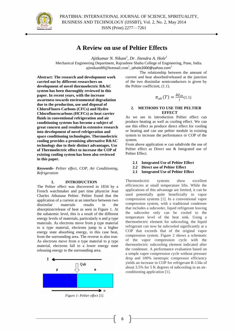
1. INTRODUCTION
The Peltier effect was discovered in 1834 by a
French watchmaker and part time physicist Jean
Charles Athanase Peltier. Peltier found that the
application of a current at an interface between two
dissimilar materials results in the
absorption/release of heat as seen in Figure 1. At
the subatomic level, this is a result of the different
energy levels of materials, particularly n and p type
materials. As electrons move from p type material
to n type material, electrons jump to a higher
energy state absorbing energy, in this case heat,
from the surrounding area. The reverse is also true.
As electrons move from n type material to p type
material, electrons fall to a lower energy state
releasing energy to the surrounding area.
Figure 1- Peltier effect [1].
The relationship between the amount of
current and heat absorbed/released at the junction
of the two dissimilar semiconductors is given by
the Peltier coefficient, (1.1).
𝜋𝑎𝑏 𝑇 =∆𝑄𝑎𝑏
𝐼(1.1)
2. METHODS TO USE THE PELTIER
EFFECT
As we see in introduction Peltier effect can
produce heating as well as cooling effect. We can
use this effect as produce direct effect for cooling
or heating and can use peltier module in existing
system to increase the performance or COP of the
system.
From above application w can subdivide the use of
Peltier effect as Direct use & Integrated use of
Peltier Effect.
2.1 Integrated Use of Peltier Effect
2.2 Direct use of Peltier Effect
2.1 Integrated Use of Peltier Effect
Thermoelectric systems show excellent
efficiencies at small temperature lifts. While the
applications of this advantage are limited, it can be
used potentially quite beneficially in vapor
compression systems [1]. In a conventional vapor
compression system, with a traditional condenser
that includes a subcooler, liquid refrigerant leaving
the subcooler only can be cooled to the
temperature level of the heat sink. Using a
thermoelectric element for subcooling, the liquid
refrigerant can now be subcooled significantly at a
COP that exceeds that of the original vapor
compression system. Figure 2 shows a schematic
of the vapor compression cycle with the
thermoelectric subcooling element indicated after
the condenser. A performance evaluation based on
a simple vapor compression cycle without pressure
drop and 100% isentropic compressor efficiency
yields an increase in COP for refrigerant R-134a of
about 3.5% for 5 K degrees of subcooling in an air-
conditioning application [1].

PRATIBHA: INTERNATIONAL JOURNAL OF SCIENCE, SPIRITUALITY,
BUSINESS AND TECHNOLOGY (IJSSBT), Vol. 2, No. 2, May 2014
ISSN (Print) 2277—7261
7
Figure 2- Schematic of vapor compression cycle with TE subcooler [1].
Figure 3- Performance enhancement with subcooling [1]
As result comes, from COP peaks according to
Figure 3a at 15 K degrees of subcooling at about
20% capacity increase according to Figure 3b, the
capacity keeps increasing to about 40% at 35 K
degrees of subcooling [1]. Peltier effect also used
in application of thermoelectric devices to enhance
the performance of air-cooled heat exchanger [2].
Thermoelectric devices are capable of converting
electrical energy into thermal heat-pumping at a
very high efficiency [2].
In this application TE device in a part of a
coil to investigate the improvement potential. A
schematic of a TE enhanced air-cooled heat
exchanger is shown in Figure 4. A half cross
section of a tube-fin heat exchanger is shown in
Figure 4 along with a TE element placed between
the fins and the tube. The power supply
connections for the TE element are not shown for
simplicity.
Figure 4- Schematic of a TE enhanced tube-fin heat
exchanger [2].
From Figure 5 it can be seen that with
relatively low power consumption the TE element
is able to provide temperature lifts of more than
10K. Comparing the heat transferred per fin with
the power consumption, it is possible to calculate a
coefficient of performance for the TE device. From
Figures 5a and 5b, an optimal value of temperature
lift can be chosen for a given application.
Figure 5- Simulation results - effect of TE device power
consumption [2].
The experiments show that when a TE device is
used as a dedicated subcooler at the condenser
outlet, a 16.2% increase in system COP and over
20% increase in cooling capacity can be achieved.
This also means when designing a system for a
given capacity and application, it is possible to
significantly reduce the heat exchanger sizes
thereby reducing the cost of the system [2].

PRATIBHA: INTERNATIONAL JOURNAL OF SCIENCE, SPIRITUALITY,
BUSINESS AND TECHNOLOGY (IJSSBT), Vol. 2, No. 2, May 2014
ISSN (Print) 2277—7261
8
Thermoelectric (TE) modules have been integrated
into a subcooler of an experimental CO2
transcritical vapor compression cycle test system
[3].The TE Subcooler was designed and fabricated
to subcool CO2 exiting the gas cooler to a
temperature below ambient. The heat from the TE
Subcooler was rejected to the ambient utilizing a
separate thermosyphon refrigerant loop with a
separate condenser. The thermoelectric modules
operate at efficiencies greater than the baseline
system, increasing capacity and the overall
coefficient of performance (COP) of the entire
system. Figure 6 shows the A small CO2
transcritical vapor compression cycle was built to
test the potential performance improvement of a
TE Subcooler utilizing a prototype compressor
with a cooling capacity of roughly 1 kW.
Figure 6 - Schematic of the experimental setup [3].
The TE Subcooler was aligned vertically, with
CO2 entering at the top from the gas cooler and
exiting at the bottom to the expansion valve. The
thermosyphon refrigerant, in this case R22, boils
within the heat rejection microchannels. The vapor
refrigerant travels upward to the thermosyphon
condenser, where it condenses and travels back to
the inlet of the heat rejection microchannels at the
bottom of the TE Subcooler. In the original system
setup the thermosyphon condenser was integrated
into the gas cooler utilizing the same set of fans.
Initial testing showed that this significantly
reduced the capacity of the gas cooler and resulted
in a negligible system performance improvement.
In subsequent testing the thermosyphon condenser
was separated from the gas cooler employing a
second fan. For above experimental setup a listed
system performance as shown in below table no. 1
System Baseline System
(Maximum COP)
TE System
(Maximum COP)
TE System
(Maximum Capacity)
System COP 2.354 2.476 (+5.2%) 2.379 (+1.1%)
System Capacity (kW) 1.44 1.569 (+9.2%) 1.657 (+15.3%)
Discharge Pressure (kPa) 9553 9042 9206
Compressor Power (kW) 0.61 0.591 0.601
Mass Flow Rate (g/s) 9.9 10.2 10.1
TE Supply Current (Amps) - 4 6
Number of Modules - 10 10
TE Capacity (kW) - 0.204 0.256
TE COP - 4.839 2.676
GC/TE Outlet Temperature (°C) 36.6 33.9 31.9
Table 1- Baseline and TE Subcooler system performance at a suction pressure of 4,198 kPa [3].
Performance improvement of a CO2 transcritical
cycle utilizing a TE Subcooler was experimentally
demonstrated. An increase in COP of 5% was
achieved with a corresponding 9% increase in
capacity. A capacity improvement of 15% was
achieved at comparable COP as the baseline
system [3].
2.2 Direct use of Peltier Effect
Refrigeration effect can be produce by direct use
of Peltier Modules [5]. To obtain such effects
thermoelectric refrigerator with an inner volume of
55 X 103 m
3 has been designed and tested, whose
cold system is composed of a Peltier pellet (50 W
of maximum power) and a fan of 2 W. An

PRATIBHA: INTERNATIONAL JOURNAL OF SCIENCE, SPIRITUALITY,
BUSINESS AND TECHNOLOGY (IJSSBT), Vol. 2, No. 2, May 2014
ISSN (Print) 2277—7261
9
experimental analysis of its performance in
different conditions has been carried out [5].A
thermal scheme of the thermoelectric refrigerator
and a photograph of the prototype are respectively
shown in Figs. 7 and 8. The Peltier pellet is
supplied with a continuous current (Vmax = 12 V)
so that heat is liberated by one side and absorbed
by the other one. The firstlaw of thermodynamics
for steady state (expressed by powers) applied to a
refrigerating machine, is the following:
𝑄 𝐻 + 𝑊 𝑒 = 𝑄 𝑐
Figure 8- Photograph of the thermoelectric refrigerator
[5]
Figure 7- Thermal sketch of the thermoelectric
refrigerator [5].
For instance: lower level of noise and vibrations, a
greater useful life, it does not use refrigerants and
provides a greater control of temperatures. A
thermoelectric refrigerator with an inner volume of
55 X 103 m
3 has been designed and built. It needs a
continuous electric current (maximum 12 V) what
makes it suitable for automobile industry
applications, since it offers the following
advantages with respect to vapour compression
[5]:
A more ecological system because it does
not use refrigerants.
More silent and robust since it minimizes
the moving parts (it does not need a
compressor).
More precise in the control of
temperatures, since it does not need to
carry out start–stop cycles, making it
possible to vary the supply voltage in a
progressive way.
The main disadvantage is linked to the electricity
consumption. The electric energy consumed by a
thermoelectric refrigerator is higher in comparison
with current compression refrigerators
(approximately the same as a vapour compression
one with an inner volume of 100 X 103 m
3). Peltier
effect also has been used directly to produce the
refrigeration Effect [6]. This can be experimentally
shown by creating the setup as shown in fig. 9. The
main body of the refrigeration chamber has a
dimension of: 0.11x0.29x0.33 m³ strongly
insulated to minimize heat loss to the ambient air.
In the cross section of this chamber, three layers
exist: two walls of aluminum separated by an
insulating material of 3 cm of thickness. Refer to
figure 9
.
Figure 9- Main body of the refrigeration
chamber [6].
High density heat sinks were specially fabricated
for this project. They are made of Aluminum and
are 350 x 75 x 39 mm³, with 21 fins along their
length and weight is 1500 Grams. Their specific
heat is 0.963 J/g.°C. The ―hot‖ surface of the
thermoelectric heat pump must be attached to a
heat sink that is a capable of carrying away both
the heat pumped by the modules and the heat
generated by the Joule effect [6]. The ―cold‖
surface is also attached to another heat sink that
will carry away the cold air, hence decreasing the
temperature differential _T, and then making the
thermoelectric more efficient. A ―spacer block‖ is
also put between the modules and the heat sinks.
Its thickness, of 18 mm, separates the ―hot‖ heat
sink from the ―cold‖ one, which yields to a
maximum heat transfer. The refrigeration chamber
was run for many values of input current. The
temperature, time and input electrical power were
measured. The obtained COP for the different
current is shown in table 2.

PRATIBHA: INTERNATIONAL JOURNAL OF SCIENCE, SPIRITUALITY,
BUSINESS AND TECHNOLOGY (IJSSBT), Vol. 2, No. 2, May 2014
ISSN (Print) 2277—7261
10
Input Current (A)
Input
Power (W)
Output
Power (W)
COP(Experi
mental)
1 12.89 24.61 1.91
2 52.62 43.06 0.818
3 119.58 55.37 0.463
4 216.56 55.38 0.255
Table 2-Cooling Performance Results [6].
Peltier Effect can be directly use in Air
conditioning Duct in supply & return way [7].
The design planning was conducted for an
office space for personal use and used the acrylic
board (height at 50cm, width at 100cm and height
at 80cm) to make the personal office activity
space, on which the single duct and double duct air
adjusting devices were installed, as shown in
Figure 10
Figure 10- Single duct air-conditioning system and double duct air-conditioning system design [7].
In the channel, the return air inlet and air outlet
were designed. The air inside the air-conditioning
is driven by the cycling fan to enter from the return
air inlet into the air adjusting devices and come out
of the air outlet after temperature adjustment into
the air-conditioned space. In the air adjusting
device, four cooling chips were installed. On the
cold side of the chip, heat exchanging fins are
installed, by which the air can be cooled. On the
hot side of the chip, water cooling component is
installed to take away the high temperature heat by
water cycling.
In this experiment , regarding the
proposed single duct and double duct personalized
air-conditioning systems, when the ambient
temperature was 29℃, the air outlet temperature
was 22℃, 24℃ respectively, and power
consumption was 133W, 134W respectively[7].
Peltier effect can also use as
thermoelectric radiant air-conditioning (TE-RAC)
system, which employs the thermoelectric modules
as radiant panels instead of conventional hydronic
panels [8].As shown in Fig.11 Thermoelectric
Modules is used directly for the space cooling
purpose
. Figure 11-Schematic of the virtual office space and its associated TE-RAC system [8]

PRATIBHA: INTERNATIONAL JOURNAL OF SCIENCE, SPIRITUALITY,
BUSINESS AND TECHNOLOGY (IJSSBT), Vol. 2, No. 2, May 2014
ISSN (Print) 2277—7261
11
In the above TE-RAC system, the thermoelectric
modules work as radiant panels by taking electrical
current. The novel system has a lot of advantages
including Freon free, convenient installation, no
complex water distribution pipes, convenient
switch between cooling and heating modes, quiet
and reliable operation due to no moving part,
etc.[8]
A thermoelectric device was used to control the
temperature of the car-seat surface: the warm
temperature in the summer and cold temperature in
the winter. The characteristics of the
thermoelectric device for the car-seat were
analyzed in relation to the input voltage and output
temperature of the device [9].
Figure 12- Appearance of developed car-seat system
[9].
We developed a car-seat system comprised of the
air conditioning system utilizing the thermoelectric
devices as shown in Fig. 12. The car-seat system is
composed of two temperature control modules,
each attached with two thermoelectric devices, as
shown in Fig. 12. The two modules were placed in
parallel, as shown in Fig. 12. In all, four
thermoelectric devices HM3930 were placed at a
sufficient distance to avoid mutual heat
conduction. Temperature sensors were placed
closest to the device since they cannot be placed on
the plate, and the sensors were bonded at the thin
copper plate to conduct the heat between the
human body and the device. An insulating material
was used to prevent heat conduction from the
warm side to the cool side and human body.
Figure 13- Performance test result of car-seat system
[9].
Fig. 13shows the result of the temperature
test on the car-seat system. Two thermoelectric
devices were connected in series to supply 6 V to
each device since the supply voltage from the car
battery is 12 V. By the serial connection of two
same devices, the supply voltage input to the
device became 6 V. Although the temperature of
the car-seat is balanced by the temperature control
module using the air conditioning system, the
temperature equilibrium can be upset, and without
a robust temperature control system, the
temperature can easily increased due to the
external conditions.
In traditional way we use natural
convection which gives the uneven cooling, leads
to generate the hot pocket & results in reduction of
the efficiency of the electrical system.
Following system shows direct use of
peltier effect to reduce the temperature which is
generated during the working of electronic devices.
We can use this peltier module externally or
internally as per requirement, shown in below
figure 14.
Figure 14 - Single thermoelectric cooler
mounted externally, internally [10].
CONCLUSION –
There are several different types of cooling devices
available to remove the heat from industrial
enclosures, but as the technology advances,
thermoelectric cooling is emerging as a truly viable
method that can be advantageous in the handling
of certain small-to-medium applications. As the
efficiency and effectiveness of thermoelectric
cooling steadily increases, the benefits that it
provides including self-contained, solid-state
construction that eliminates the need for
refrigerants or connections to chilled water
supplies, superior flexibility and reduced
maintenance costs through higher reliability will
increase as well.
REFERENCES- [1] Reinhard Radermacher, Bao Yang,Integrating
Alternativeand ConventionalCooling Technologies, ASHRAE Journal, October 2007.
[2] Jonathan Winkler, Potential Benefits of Thermoelectric Element Used With Air-Cooled Heat
Exchangers, International Refrigeration and Air Conditioning Conference, 2006.

PRATIBHA: INTERNATIONAL JOURNAL OF SCIENCE, SPIRITUALITY,
BUSINESS AND TECHNOLOGY (IJSSBT), Vol. 2, No. 2, May 2014
ISSN (Print) 2277—7261
12
[3] Jonathan Schoenfeld, Integration of a Thermoelectric Subcooler Into a Carbon Dioxide
Transcritical Vapor Compression Cycle
Refrigeration System, International Refrigeration and Air Conditioning Conference,2008.
[4] Michael Ralf Starke, Thermoelectrics for Cooling
Power Electronics, The University of Tennessee, Knoxville,2006.
[5] D. Astrain, J.G. Via´n, J. Albizua, Computational model for refrigerators based on Peltier effect
application, Applied Thermal Engineering 25
(2005) 3149–3162.
[6] Chakib Alaoui, Peltier Thermoelectric Modules
Modeling and Evaluation, International Journal of Engineering (IJE), Volume (5) : Issue (1) : 2011
[7] Tsung-Hsin Hung, Construction and Analysis of
Personalized Air-conditioning System, National Chin Yi University of Technology, Taichung City
41170, Taiwan.
[8] Limei Shen, Investigation of a novel thermoelectric radiant air-conditioning system, Energy and
Buildings 59 (2013) 123–132.
[9] Hyeung-Sik Choi, Development of a temperature-controlled car-seat system utilizing thermoelectric
device, Applied Thermal Engineering 27 (2007) 2841–2849
[10] Judith Koetzsch & Mark Madden, Thermoelectric Cooling for Industrial Enclosures,
Rittal White Paper 304.

PRATIBHA: INTERNATIONAL JOURNAL OF SCIENCE, SPIRITUALITY,
BUSINESS AND TECHNOLOGY (IJSSBT), Vol. 2, No. 2, May 2014
ISSN (Print) 2277—7261
13
Simulation & Parametric Finite Element Analysis for Sheet
Metal FormingProcess
Dipak C. Talele1, Dr. Dheeraj S. Deshmukh
2, Mahesh V. Kulkarni
3
1Assistant Professor, S.S.B.T.‘s, College of engineering & Technology, Bambhori, Jalgaon 2Professor & Head, S.S.B.T.‘s, College of engineering & Technology, Bambhori, Jalgaon
3Assistant Professor, S.S.B.T.‘s, College of engineering & Technology, Bambhori, Jalgaon
Abstract—Finite element analysis (FEA) is
successful in simulating complex industrial
sheet forming operations, the accurate and
reliable application of this technique to spring-
back has not been widely demonstrated. Several
physical parameters, as well as numerical,
influence this phenomenon and its numerical
prediction.
In this paper, the effect of blank Thickness,
blank holding force, Material, coefficient of
Friction on the spring-back of specimens are
discussed. The role that all the above
parameters play in the spring-back is assessed
through finite element simulations. Process
conditions, such as Tool geometry, working
temperature have an obvious effect on spring-
back. Simulations are conducted with varying
blank holding force, Materials, blank thickness,
and coefficient of frictions to assess its role in
spring-back of the formed part.
Keywords— blank holding force, coefficient of
Friction, finite element analysis, simulations,
spring-back,
INTRODUCTION
Spring-back is a phenomenon that occurs
in many cold working processes. When a metal is
deformed into the plastic region, the total strain is
made up of two parts, the elastic part and the
plastic part. When removing the deformation load,
a stress reduction will occur and accordingly the
total strain will decrease by the amount of the
elastic part, which results in spring-back [1].
Spring-back describes the change in shape
of a formed sheet upon removal from the tooling.
It is more severe for materials with higher
strength-to-modulus ratios (e.g., aluminium and
high strength steel (HSS)). The finite element
analysis (FEA) of spring-back is shown to be very
sensitive to many numerical parameters, including
the number of through-thickness integration points,
type of element, mesh size, angle of contact per
element on die shoulder, possible inertia effects
and contact algorithm. Moreover, spring-back is
also sensitive to many physical parameters
including material properties, hardening laws,
coefficient of friction, blank holder force (BHF)
and possible unloading procedure. All these
parameters make spring-back simulation very
cumbersome [6].
Azraq et al. [2] verified the stamping process and
the shape of the final component for studying
spring-back of AHSS. With help of examples of
analyzing spring-back using FEM, it was shown
that the analysis enables to predict the influence of
material strength. It was considered as it is possible
to decrease the spring-back in future using the
application of new FEM techniques. Tekaslan et al.
[3] determined the amount of spring-back in sheet
metals at different bending angles has been
obtained by designing a modular ‗V‘ bending die.
Also he checked the spring-back for three kinds of
materials of different thickness by using four
different bending methods on eighteen different
modular dies and a total of 720 experiments he did,
at least 10 experiments belonging to each of the
kinds. The results have shown that out of the four
different bending methods used in the field most,
two cannot be employed for spring-back. Also he
concluded that (1) holding the punch longer on the
material bent reduces spring-back (2) application
time of the punch load is important to determine
the spring-back value. (3) As bend angle increases
spring-back angle increases. Liu et al. [4] used the
optimized neural network model to predict spring-
back and they found that smaller is the material
yield strength, lower is the spring-back value. Also
conclude that spring-back value is lower as bigger
Young‘s modulus, smaller ratio of bending radius
to sheet thickness, bigger ratio of bending height to
sheet thickness, thicker sheet metal, and bigger
ratio of tool gap to sheet thickness. De Souza et al
[5] characterizes the effect of material and process
variation on the robustness of spring-back for a
semi-cylindrical channel forming operation as it
shares a similar cross-section profile of many
automotive structural components. With the help
of experiments they analyzed that variation in the
mechanical properties of the sheet material had the
maximum influence on spring-back. Kim et al. [7]
investigated the effect of temperature gradients on

PRATIBHA: INTERNATIONAL JOURNAL OF SCIENCE, SPIRITUALITY,
BUSINESS AND TECHNOLOGY (IJSSBT), Vol. 2, No. 2, May 2014
ISSN (Print) 2277—7261
14
spring-back in warm forming of lightweight
materials. Also he analyzed the dependence of
spring-back on blank holder force (BHF), friction
condition, and forming rate.
Naceur et al. [8] invested a surface response
method for the optimization of tools geometry in
sheet metal forming in order to reduce the spring-
back effects after forming. Verma et al. [9]
predicted the effect of anisotropy on spring-back
using finite element analysis for the benchmark
problem of Numisheet-2005 [2005 Numisheet
Benchmark 2, Spring-back prediction of a cross
member]. He developed an analytical model to
cross check the trends predicted from the finite
element analysis. He observed that the effective
stress has not been treated as a constant and the
radial stress is considered in the present model.
From both the models (FE and analytical),
predicted that higher anisotropy gives higher
spring-back. And Finite element analysis of the
problem shows that spring-back is minimum for an
isotropic material.
Vladimirov et al. [10] introduced the application of
a finite strain model to predict spring-back in sheet
forming. The concept combines both isotropic and
kinematic hardening and utilizes a new algorithm
based on the exponential map. A special focus is
put on the simulation of the draw-bend test of
DP600 dual phase steel sheets and the comparison
of the numerical results with experimental data.
Also, they investigated the sensitivity of the results
with respect to geometry parameters such as the
tool radius and the sheet thickness as well as the
ratio between isotropic and kinematic hardening.
He concluded that finite strain combined hardening
model is very well suited for spring-back
prediction. Panthi et al. [11] predicted the spring-
back in a typical sheet metal bending process and
to investigate the influence of parameters such
young‘s modulus, strain hardening, yield stress on
spring-back. The results of simulation are validated
with his own experimental results. He concluded
that Friction has negligible effect on spring-back.
The spring-back increases with increase in yield
stress.
PROBLEM DESCRIPTION
Let us start with a description of the problem we
will study throughout this paper, namely the U-
draw bending. It is very useful for our study since,
on the one hand, it is very sensitive to many
parameters from both the experimental and the
numerical point of view and, on the other hand,
spring-back can be quantified by three simple
geometric measurements.
The schematic drawing of the U-draw bending
is shown in Fig. 1. The Dimensions are given in
table 1. The three geometric quantities that
quantify spring-back are shown in Fig. 2. These
consist of two angles θ1 and θ2 and the radius r.
Fig.1. Schematic U-draw bending process
Dimension
s Die Punch
Binder
s Blank
Length
(mm) 300 58 55 300
Height
(mm) 80 80 10
0.9,1,1.1
(thickness
)
Width
(mm) 45 45 45 35
Corner
radius
(mm)
6 10 10 -
Table no. 1. Dimensions of the geometry
Fig.2. Description of the three quantities θ1, θ2 and r to
quantify spring-back.
The main hypotheses used throughout this
simulation are the following:
Element type: 2D linear shell element.
Time integration scheme: dynamic explicit
and static implicit.
Spring-back simulation: complete tool
removal including contact interactions.
Contact algorithm: kinematic pair method on
analytically defined rigid bodies.

PRATIBHA: INTERNATIONAL JOURNAL OF SCIENCE, SPIRITUALITY,
BUSINESS AND TECHNOLOGY (IJSSBT), Vol. 2, No. 2, May 2014
ISSN (Print) 2277—7261
15
Taking Isotropic hardening in to
consideration.
Result of simulations will be shown for the three
following materials: CRDQ Steel, DP Steel and
HSLA Steel. Materials properties are given in
Tables 2.
Table no. 2 Mechanical Properties of Material [12, 15]
True Stress Vs Plastic Strain curve for
materials are as shown in figure 3, 4 and 5.
Fig 3 Stress Vs Plastic Strain curve for DP Steel [12]
Fig 4 True Stress Vs Plastic Strain curve for CRDQ
Steel [15]
Fig 5 True Stress Vs Plastic Strain curve for HSLA
Steel [15]
SIMULATION PROCESS
In the simulations performed, special attention
is given in order to remain as close as possible to
the physical process. Using a dynamic explicit and
static implicit time integration scheme, we are able
to simulate the whole process including both the
loading and the unloading phases with the two
time integration algorithm and with a frictional
contact algorithm active all along the process. The
start to end process is described in Fig. 6. Figure 7
represent the final condition of component after
spring-back operation.
Name of Material Properties Dual Phase Steel CRDQ Steel HSLA Steel
Young‘s Modulus 205.35 GPa 210 GPa 210 GPa
Poisson‘s Ratio 0.3 0.3 0.3
Yield strength (0.2% offset) 358.7 MPa 185 MPa 586 MPa
𝑟00 Lankford coefficient 0.79 1.6 1
𝑟45 Lankford coefficient 1.03 1.6 1
𝑟90 Lankford coefficient 1.01 1.6 1

PRATIBHA: INTERNATIONAL JOURNAL OF SCIENCE, SPIRITUALITY,
BUSINESS AND TECHNOLOGY (IJSSBT), Vol. 2, No. 2, May 2014
ISSN (Print) 2277—7261
16
Fig 6 Deformed shapes before spring-back at
different time
Fig 7 deformed shape after spring-back
RESULTS AND DISCUSSION
Different 81 simulation cases were done during
analysis, taking different material, blank holding
forces, coefficient of friction, and blank
thicknesses to analyze their effect on spring-back.
Effect of material on Spring-back:
From figures 8-10, it is observed that spring-back
increases as the strength of material increases. This
is because as strength of material increases elastic
recovery increases which implies increase in
spring-back.
Fig.8 Blank Holding Force Vs θ1
Fig.9 Blank Holding Force Vs θ2
Fig.10 Blank Holding Force Vs ρ
Effect of the BHF
We will now study the influence of several
physical and numerical parameters on spring-back.
The first of those is the BHF. It is experimentally
observed that the spring-back increases with small
forces, but decreases as the force increases for
large force values. The same phenomenon is found
in the FE simulation using different types of steel
as shown in Figs. 8-10. The curves exhibit an
extremum for some values of the BHF and one can
also find a BHF value where the considered
spring-back parameter almost vanishes. This
phenomenon can be explained by the fact that with
low BHF, the punch induces mostly bending
stresses in the material, but as the blank holder
holds the blank more severely, the stresses induced
by the punching phase become mostly tensile
stresses.
Effect of the coefficient of friction
Friction is an important but not very well known
factor influencing spring-back. Its modelling is
difficult because this coefficient is probably
different on the curved and flat parts of both the
die and punch.

PRATIBHA: INTERNATIONAL JOURNAL OF SCIENCE, SPIRITUALITY,
BUSINESS AND TECHNOLOGY (IJSSBT), Vol. 2, No. 2, May 2014
ISSN (Print) 2277—7261
17
Fig. 11 Coefficient Of Friction Vs θ1
Fig. 12 Coefficient Of Friction Vs θ2
Fig. 11 Coefficient Of Friction Vs ρ
A. Moreover, it is very difficult to measure those
coefficients experimentally. So, we have
chosen to use the same coefficient on all parts
of all the tools and study the results obtained
for different values. Figs. 11–13 show that the
same behaviour as for BHF is observed: spring-
back curves also exhibit an extremum (we used
different types of thicknesses for this case).
Effect of the Material thicknesses
From figures 11-13, it is observed that spring-back
increase with decrease in blank thickness. This is
because as thickness of blank increases, plastic
deformation of blank increases.
Conclusions
In this paper, a spring-back prediction is described
using simulation and the results obtained are
compared with experimental data. A simulation
method describing the blank shape during the
whole process is introduced. The influence on
spring-back of several parameters such as BHF,
coefficient of friction, Blank thickness, and
Material used were studied in details.
References [1] Ihab Ragai, Duraid Lazim, James A. Nemes, ―Anisotropy
and springback in draw-bending of stainless steel 410 experimental and numerical study‖, Journal of Materials
Processing Technology 166 (2005) 116–127.
[2] S. Al Azraq, R. Teti, J. Costa, ―Springback prediction with FEM analysis of advanced high strength steel
stamping process‖, Dept. of Materials and Production Engineering, University of Naples Federico II, Naples,
Italy.
[3] Ozgur Tekaslan, Nedim Gerger, Ulvi Seke,
―Determination of spring-back of stainless steel sheet
metal in ‗‗V‘‘ bending dies‖, Materials and Design 29
(2008) 1043–1050.
[4] Wenjuan Liu , Qiang Liu, Feng Ruana, Zhiyong Liang,
Hongyang Qiu, ―Spring-back prediction for sheet metal forming based on GA-ANN technology‖, Journal of
Materials Processing Technology 187–188 (2007) 227–
231.
[5] T. deSouza, B.F.Rolfe, ―Characterizing material and
process variation effects on spring-back robustness for a semi-cylindrical sheet metal forming process‖,
international Journal of Mechanical Sciences 52 (2010)
1756–1766.
[6] Luc Papeleux, Jean-Philippe Ponthot, ―Finite element
simulation of springback in sheet metal forming‖, Journal of Materials Processing Technology 125–126 (2002) 785–
791.
[7] Hong Seok Kim, Muammer Koc¸ ―Numerical investigations on springback characteristics of aluminium
sheet metal alloys in warm forming conditions‖, journal of
materials processing technology 204 ( 2008 ) 370–38.
[8] H. Naceur, Y.Q. Guo , S. Ben-Elechi, ―Response surface
methodology for design of sheet forming parameters to control springback effects‖, Computers and Structures 84
(2006) 1651–1663.
[9] Rahul K. Verma , A. Haldar, ―Effect of normal anisotropy on spring-back‖, Journal of Materials Processing
Technology 190 (2007) 300–304.
[10] I.N. Vladimirov, M.P. Pietryga, S. Reese, ―Prediction of
springback in sheet forming by a new finite strain model with nonlinear kinematic and isotropic hardening‖,
Journal of Materials Processing Technology 209 (2009)
4062–4075.
[11] S.K. Panthi, N. Ramakrishnan, Meraj Ahmed, Shambhavi
S. Singh, M.D. Goel, ―Finite Element Analysis of sheet
metal bending process to predict the spring-back‖, Materials and Design 31 (2010) 657–662.
[12] peng cheng, MuammerKoc, ―Simulation of springback
variation in forming of advanced high strength steels‖,
Journal of Material Processing Technology 190 (2007)
189-198.
[13] Myoung-Gyu Lee, Daeyong Kim, Chongmin Kim,
Michael L.Wenner, Kwansoo Chung., ―Springback Evaluation of automotive sheets based on isotropic-
kinematic hardening laws and non-quadratic anisotropic
yield functions, part 3:- Applications‖, International Journal of Plasticity 21 (2005) 915-953.
[14] http://cdn.intechopen.com/pdfs/12099/InTech
[15] Radioss Theory Manual, Version 10.0, January-2009.
ABAQUS-6.11 Help Manual

PRATIBHA: INTERNATIONAL JOURNAL OF SCIENCE, SPIRITUALITY,
BUSINESS AND TECHNOLOGY (IJSSBT), Vol. 2, No. 2, May 2014
ISSN (Print) 2277—7261
18
Effect of Biofilm in Waste Water Treatment by Using
Bactericidal Activity of Nitrogen Doped Metal Oxide
Nanoparticles
I. D. Patil *1, Yogita Patil
2, Mayur Ladole
3.
1Department of Biotechnology SSBT‘s COET, Jalgaon-425001. India.
2Department of Biotechnology, Government College of Engineering, Jalgaon-425001. India.
3Department of Biotechnology, SSBT‘s COE, Jalgaon-425001. India.
Abstract
Background: Biofilm of different microorganisms
can stabilize harmful components from waste
water. It can be effectively use for the treatment of
waste water.
Objective: Development of Rotating Drum
Biological Reactor (RDBR) for the treatment of
waste water and to study the effect of biofilm
developed on RBDR for the reduction in BOD,
COD and phenol concentration in waste water.
Synthesis of TiO2 nanoparticles to study
antimicrobial property against developed biofilm.
Results: Synthetic waste water with initial
concentration of phenol as 50 mg/lit and with COD
and BOD values 2080 mg/lit and 1600 mg/lit
respectively was treated in RDBR. After 60 hrs of
operation phenol concentration drops to 0.0028
mg/lit and COD, BOD values were reduced to 178
mg/lit and 71.2 mg/lit respectively. The reduction
of phenol concentration was upto 99.7%.
Conclusion: Based on the experimental results we
can conclude that rotating drum biological reactor
(RDBR) technology is one of the promising
technology for the treatment of waste water. After
treatment of synthetic waste water in RDBR there
was drastic reduction in the initial concentrations of
COD, BOD and Phenol was observed. Results
show the reduction in phenol concentration upto
99.7%. It has been also found that nitrogen doped
TiO2 nanoparticles shows good antimicrobial
activity over the biofilm developed.
INTRODUCTION
Water is the most important constituent for all the
living things. Water contamination is now a major
problem in the global context as a consequence of
industrialization, globalization, population growth,
urbanization and warfare combined with increased
wealth and more extravagant lifestyles (UN- World
Water Development Report, 2006). Eutrophication
of lakes and the sea is caused by discharge of
nutrients originating from of human activities,
industries and agriculture, which threatens the
maintenance of biodiversity and human health.
Suspended, colloidal or dissolved degradable
organic materials, quantities and ratios depend on
the nature of the wastewater characteristics of
wastewater are measured in terms of chemical
oxygen demand (COD), Biological oxygen demand
(BOD), and volatile suspended solid (VSS).
Biological wastewater treatment is therefore of
utmost importance for the wellbeing of our water
bodies. Biological treatment is one of the most
widely used removal methods as well as for partial
or complete stabilization of biologically degradable
substances in wastewater and wastes. Most
biological waste and wastewater treatment
processes employ bacteria as primary micro-
organisms; certain other micro-organisms may play
an important role. Degradation of organic matter is
effected by its use as food by micro-organisms to
produce protoplasm for new cells during the growth
process, population dynamics of bacteria is
biological treatment depends on environmental
factors which include pH, temperature, type and
concentration of essential nutrients (e.g. Nitrogen,
Phosphorous, Sulphur etc.), essential minerals,
osmotic pressure, media toxicity, by-products and
degree of mixing.A biofilm can be defined as a
complex coherent structure of cells and cellular
products, like extra-cellular polymers (Characklis,
1990), which either form spontaneously as large,
dense granules (Lettinga et al., 1980), or grow
attached on a static solid surface (static biofilms) or
on suspended carriers (particle supported biofilms)
(Heijnen, 1984). Biological wastewater treatment is
mainly carried out by prokaryotes, even if fungi,
protozoa, algae and rotifers may also be represented
(Bitton G, 2005). Municipal wastewater is
composed of organic material, i.e. proteins,
carbohydrates, fats and oils; nutrients, mainly
nitrogen and phosphorus; as well as trace amounts
of recalcitrant organic compounds and Metals
(Bitton G, 2005).
The most frequently found prokaryotes in
biological wastewater treatment systems belong to
the classes Alpha-, Beta- and Gamma
proteobacteria, Bacteroidetes and Actinobacteria
(Wagner M and Loy A, 2002).These bacteria in
aquatic environments are predominantly not in a
free-floating planktonic stage, but have a tendency
to attach to surfaces and form multi-species
communities called biofilms (Metcalf & Eddy,

PRATIBHA: INTERNATIONAL JOURNAL OF SCIENCE, SPIRITUALITY,
BUSINESS AND TECHNOLOGY (IJSSBT), Vol. 2, No. 2, May 2014
ISSN (Print) 2277—7261
19
1991; Syron & Casy, 2007). The microbes produce
extracellular polymeric substances (EPS), which
form complexes with the surface materials
(Andersson S et al., 2009). A mature biofilm is a
complex mixture of active and dormant or drying
cells, inorganic and organic materials and tunnels
filled with water, and the biofilm contains both
aerobic and anaerobic niches (Korber et al., 1995;
O‘Toole et al., 2000).
The most commonly used process for the treatment
of municipal and industrial waste water is activated
sludge process, but increasingly biofilm
technologies are utilized. Biofilm waste water
treatment processes can be roughly divided into 1)
the fixed-medium systems, and 2) moving-medium
systems (Rodgers et al., 2003). In the fixed-medium
systems (fixed bed bioreactor; FBBR) the
biological reactions take place in the biofilm
growing on a static medium. In the moving medium
systems the biofilm media are kept in continuous
movement by mechanical, hydraulic or air forces.
Rotating bed bioreactors (RBBR) are an application
of moving bed biofilm reactors with a higher filling
rate of carrier elements.
Nanoparticles in waste water treatment:
The waste water treatment plant in which trickling
filter, RBC, packed bed reactor are used involve
formation of biofilm, which reduces the COD of
treated water (Nicholas P. Cheremisinoff,2003).
More recently, several natural and engineered
nanomaterials have also been shown to have strong
antimicrobial properties, including chitosan (Qi et
al., 2004), silver nanoparticles (nAg) (Morones et
al., 2005), photocatalytic TiO2 (Cho et al., 2005;
Wei et al., 1994), fullerol (Badireddy et al., 2007),
aqueous fullerene nanoparticles (nC60) (Lyon et
al., 2006), and carbon nanotubes (CNT) (Kang et
al., 2007).
The biofilm form during water treatment process
can be stabilised/ degraded by using the metal
oxide nanoparticles such as TiO2, the surface of
TiO2 crystal is occupied by O2 atoms with high
electron density. The bactericidal effect of TiO2 is
attributed to the decomposition of bacterial outer
membranes by reactive oxygen species [ROS],
primarily hydroxyl radicals [*OH] which leads to
phospholipids peroxidation and ultimately cell
death.
Nitrogen Doping Of Metal Oxide Nanoparticles:
TiO2 is the most commonly used semiconductor
photocatalyst.Among the different nanomaterials, it
is the most studied. Activated by UV-A irradiation,
its photocatalytic properties have been utilized in
various environmental applications to remove
contaminants from both water and air (Gelover et
al., 2006; Murray et al., 2007; Salthammer and
Fuhrmann, 2007). A wealth of information on TiO2
photocatalytic inactivation of bacteria has been
acquired over the last 20 years (Matsunaga et al.,
1985; Wei et al., 1994). TiO2 can kill both Gram-
negative and Gram-positive bacteria, although
Gram-positive bacteria are less sensitive due to
their ability to form spores (Wei et al., 1994). More
recently, nano-sized TiO2 was also reported to kill
viruses including poliovirus 1 (Watts et al., 1995),
hepatitis B virus (Zan et al., 2007), Herpes simplex
virus (Hajkova et al., 2007), and MS2
bacteriophage (Cho et al., 2005). The concentration
of TiO2 usually required to kill bacteria varies
between 100 and 1000 ppm, depending on the size
of the particles and the intensity and wavelength of
the light used (Wei et al., 1994).
An attractive feature of TiO2 photocatalytic
disinfection is its potential to be activated by visible
light, e.g. sunlight. Metal doping has long been
known to improve visible light absorbance of TiO2
(Anpo et al., 2001), and increase its photocatalytic
activity under UV irradiation (Choi et al., 1994).
Materials and Methods
Materials:
Potassium Dichromate (K2Cr2O7), Sulphuric acid
(H2SO4), Sodium thiosulfate, Starch, Phosphate
buffer solution and allylthiourea solution (0.5%)
were purchased from Merck Specialties Private
Limited (Mumbai, India). Titanium isopropoxide
(Ti (OCH (CH3)2)4) and ethanolamine were
purchased from Sigma Aldrich. All the other
chemicals used were of analytical grade with
highest purity.
Organisms and culture maintenance:
Bacillus subtilis (NCIM 2549), Pseudomonas
putida (NCIM 2847), Nocardia
hydrocarbonoxydance (NCIM 2386), Pseudomonas
aeruginosa (NCIM 2074) and Rhodococcus terrae
(NCIM 5126) were obtained from National
Collection of Industrial Microorganisms (NCIM),
Pune, India. All microorganisms are maintained on
nutrient agar slant at 40C and these are subcultured
at regular interval in departmental laboratory.
Pure Culture and Mix Culture:
Each microorganism were grown in a nutrient broth
separately and incubated for 24 hrs at 370C each in
100 ml conical flask. The inoculums were taken
from each flask and mix culture was developed in
500 ml conical flask.
Biofilm development on different materials:

PRATIBHA: INTERNATIONAL JOURNAL OF SCIENCE, SPIRITUALITY,
BUSINESS AND TECHNOLOGY (IJSSBT), Vol. 2, No. 2, May 2014
ISSN (Print) 2277—7261
20
All the flasks from the above procedure were
subjected to flask level study. In this strips of
different material such as PVC, GI, Glass, and
Nylon fiber was taken. The best optimum condition
such as pH, temperature, dilution and material will
be selected from above study and the selected
material was used for fabrication of drums which
was used in rotating drum biofilm reactor
(RDBR).
Determination of Chemical Oxygen Demand (COD):
COD is a measure of the capacity of water to
consume O2 during the decomposition of organic
matter and the oxidation of inorganic chemicals such
as ammonia and nitrite .COD was calculated
according to the method given in the book of
S.S.Dara (1999).
Phenol estimation:
The standard brominating solution is a mixture of
potassium bromide and potassium bromated
(KBr+KBrO3). The bromine (Br2) liberated from
these solution in the presence of concentrated HCL,
phenol undergoes bromination to form 2, 4, 6
tribromophenol. The excess of bromine which is not
used by phenol reacts with KI solution and liberate
iodine. The liberated iodine was titrated against
standard 0.1 N Sodium thiosulfate solution. Thus the
phenol was estimated by calculating the amount of
bromine consumed during the reaction in terms of
0.1 sodium thiosulphate solution.
Determination of Biological Oxygen Demand
(BOD):
Biological oxygen demand or BOD represents the
quantity of oxygen required by bacteria and other
micro organisms during the biochemical degradation
and transformation of organic matter present in
waste water under aerobic conditions. BOD test is of
great value in the analysis of sewage, highly polluted
waters and industrial effluents. BOD was calculated
according to the method given in the book by
S.S.Dara (1999).
Biofilm development:
For the biofilm development different materials can
be used as attachment surface but PVC
(polyvinylchloride) gives good result for attachment
of biofilm. The mix cultures of bacteria was taken
and pour in rotating drum biological reactor (RDBR)
which was made from one and half liter of PVC jar
with provision of inlet and outlet and centrally
located shaft carrying PVC drum with filter. A batch
of 500 ml mix culture was run for 7 to 8 days at 2
rpm at room temperature.
Preparation of Synthetic Waste Water:
Synthetic waste water of following constituents was
prepared. The constituent such as bacto-peptone,
MgSO4.7H2O, MnSO4.H2O, FeCl3.6H2O, CaCl2,
KH2PO4, and K2HPO4 were used to enhance the
bacterial growth (Table-1).
Table-1. Concentration of different components in
synthetic waste water
Preparation of TiO2 nanoparticles:
Nanoparticles were synthesized according to the
process shown in the Fig.1.
Chemicals- Precursor solution of 4 ml Titanium
isopropoxide (Ti (OCH (CH3)2)4) (Sigma Aldrich
97%), ethylene diamine (Strem, 99%) or
ethanolamine (Sigma Aldrich, 99%) and 200 ml of
anhydrous ethanol.
The precursor solution was refluxed for 24 hrs and
hydrolyzed by adding drop wise 20 ml distilled
water. The yellow precipitate then centrifuge and
dry under vacuum. The resulting powder then
sintered in the air at 200 0C for 1 hr.10ml of Ti
(OCH (CH3)2)4 and isopropyl alcohol (5:95 volume
ratio) was slowly added into 100ml of distilled
water at pH 2, adjusted by HNO3. The mixture was
stirred for 12 hrs: and centrifuged. The precipitates
then wash and dry under vacuum, and kept in
plastic vials. Characterizations of these particles
were done by using X-RD and particle size
distribution.
Constitute
Stock
concentr
ation
(g/l)
Quantity
used
(ml/5l)
Final
concentra
tion
(mg/l)
Bacto-
peptone
32.25 27.3 352.75
MgSO4.7H2O 10.00 25.0 50.00
MnSO4.H2O 1.60 25.0 5.00
FeCl3.6H2O 0.175 25.0 1.00
CaCl2 100 25.0 3.75
KH2PO4 52.25 33.4 349.4
K2HPO4 107.00 33.4 715.56
Phenol - - 50.00

PRATIBHA: INTERNATIONAL JOURNAL OF SCIENCE, SPIRITUALITY,
BUSINESS AND TECHNOLOGY (IJSSBT), Vol. 2, No. 2, May 2014
ISSN (Print) 2277—7261
21
Reflux 4 ml of precursor solution for 24 hrs
Hydrolyze by adding drop wise 20 ml distilled
water
Yellow precipitate
Centrifuge and dry under vacuum
Powder sinter in the air at 200 ٥C (1 hr)
Kept in a plastic vials
Fig.1.-Fabrication of TiO2 Nanoparticles.
Phospholipids peroxidation:
Bacterial cell suspension were kept at 4˚C prior to
the photocatalytic experiments.10 ml of bacterial cell
suspension was taken and 1 ml of 0.01 mg/lit
aqueous solution of nitrogen doped TiO2 particle
was added. Then this suspension was kept in Petri
dish under the light radiation for 6 hrs to facilate
photocatalytic activity of TiO2. Also simultaneously
second Petri dish was prepared without N2 doped
TiO2 solution.1 ml of suspension from each Petri
dish was taken and spread on two different agar plate
and label as Petri dish 1 and 2 respectively. Then
these agar plates were incubated for 24 hrs at 37 ˚C
and observed after 24 hrs.
Results and Discussions
Biofilm development:
After running the batch of 500 ml mix culture of
bacteria‘s for 7 to 8 days at 2 rpm at room
temperature, biofilm was observed after 8 days on
the surface of drum and appears as transparent and
sticky growth (Fig.2).
Fig.2-Developed biofilm on the surface of drum after 8
days at room temperature.
Treatment of Synthetic Waste Water:
Phenol and phenolic compounds found as
major constituent in effluents of many chemical
industries. 500 ml of synthetic waste water
containing 50 mg/lit of phenol and other
constituents such as K2HPO4, CaCl2 etc. was
treated in RDBR. Water was fed from inlet and
batch was operated for 48 hrs, samples are taken
from 12 hrs and concentration of COD, BOD and
phenol was measured (Fig.3, 4 and 5). It was found
that mix bacterial cultures were capable of
degrading phenol by 99.70 % approximately in 60
hrs.
Fig.3 Reduction in COD value of synthetic waste water after treatment in RDBR.The initial concentration of COD
which was 2080 mg/lit at 0 hrs was reduced to 178 mg/lit after 60 hrs.

PRATIBHA: INTERNATIONAL JOURNAL OF SCIENCE, SPIRITUALITY,
BUSINESS AND TECHNOLOGY (IJSSBT), Vol. 2, No. 2, May 2014
ISSN (Print) 2277—7261
22
Fig. 4. Reduction in BOD value of synthetic waste water after treatment in RDBR .The initial concentration of BOD
which was 1600 mg/lit at 0 hrs was reduced to 71.2 mg/lit after 60 hrs.
Fig. 5.Reduction in phenol concentration of synthetic waste water after treatment in RDBR .The initial concentration
of phenol which was 50 mg/lit at 0 hrs was reduced to 0.0028 mg/lit after 60 hrs

PRATIBHA: INTERNATIONAL JOURNAL OF SCIENCE, SPIRITUALITY,
BUSINESS AND TECHNOLOGY (IJSSBT), Vol. 2, No. 2, May 2014
ISSN (Print) 2277—7261
23
Phenol Degradation study at flask level:
A flask level study was done for estimation of
phenol concentration that can be treated by
biofilm. For these four different samples 300 ml of
synthetic waste water containing varying
concentration of phenol like 0.1, 0.2, 0.3 and 0.4
ml/lit was taken in 500 ml conical flask and
inoculated with mix culture of bacteria. Result
shows that bacterial growth can occur satisfactory
at about 0.4 ml phenol concentration and cannot
survive concentration above 0.6 ml per liter
phenol. (Table 2)
Synthesis of nitrogen doped TiO2 nanoparticles
TiO2 has strong antimicrobial activity and it can
act on wide range of microorganism. Doping of
TiO2 particles with nitrogen enhances the anti-
microbial activity and facilate use of TiO2 under
visible spectrum. Nitrogen doped TiO2 particles
were prepared by solgel method using titanium iso-
propoxide as TiO2 precursor and ethanolamine as
doping precursor. 24 hr reflux method in ethanol
can be used but vigorous mixing by stirrer can give
TiO2 nanoparticles within a 4 hrs.
Phospholipid peroxidation by Nitrogen doped TiO2
nanoparticles:
Results shows bacterial growth was observed on
Petri plate which was not treated with TiO2
solution (Fig.5). On other hand TiO2 treated
suspension does not give any growth on second
Petri plate (Fig.6).
Fig.5. Appearance of bacterial growth on agar plate
which was not treated with TiO2 nanoparticles.
Fig.6. Agar plates treated with TiO2 suspension
indicating the absence of bacterial growth.
Conclusion
Based on the experimental results we can conclude
that rotating drum biological reactor (RDBR)
technology is one of the promising technology for
the treatment of waste water. After treatment of
synthetic waste water in RDBR there was drastic
reduction in the initial concentrations of COD,
BOD and Phenol was observed. Results show the
reduction in phenol concentration upto 99.7%. It
has been also found that nitrogen doped TiO2
nanoparticles shows good antimicrobial activity
over the biofilm developed.
Acknowledgements
This research work was funded by National
Science and Technology Entrepreneurship
Development Board (NSTEDB), Department of
Science and Technology (DST), Government of
India, New Delhi.
References [1] Andersson S., Dalhammar G., Land C. J., Kuttuva Rajarao
G. (2009) Characterization of extracellular polymeric
substances from denitrifying organism Comamonas
denitrificans. Applied Microbiology and Biotechnology 82:3 p. 535-543.
[2] Anpo, M., Kishiguchi, S., Ichihashi, Y., Takeuchi, M., Yamashita, H., Ikeue, K., Morin, B., Davidson, A., Che,
M., 2001. The design and development of second-
generation titanium oxide photocatalysts able to operate under visible light irradiation by applying a metal ion-
implantation method. Res. Chem. Intermediates 27 (4–5),
459–467.
[3] Badireddy, A.R., Hotze, E.M., Chellam, S., Alvarez,
P.J.J., Wiesner, M.R., 2007. Inactivation of bacteriophages via photosensitization of fullerol
nanoparticles. Environ. Sci. Technol. 41, 6627–6632.
[4] Bitton G, (2005), Wastewater Microbiology. 3 ed. New Jersey: John Wiley and sons, inc.
[5] A book: Biofilms Volume-1. In: Characklis, W.G., Marshall, K.C. (Eds.), Biofilms, 2006, Wiley, 1990, New
York.
[6] Cho, M., Chung, H., Choi, W., Yoon, J., 2005. Different inactivation behavior of MS-2 phage and Escherichia coli
in TiO2 photocatalytic disinfection. Appl. Environ. Microbiol. 71 (1), 270–275.
[7] Choi, W., Termin, A., Hoffmann, M., 1994. The role of metal ion dopants in quantum size TiO2: correlation
Sr.
No.
Concentration
(ml/lit)
After
treatment
(ml/lit)
Phenol
degraded
(ml/lit)
1 0.1 0.00150 0.0985
2 0.2 0.00125 0.1980
3 0.3 0.00183 0.2981
4 0.4 0.00470 0.3950

PRATIBHA: INTERNATIONAL JOURNAL OF SCIENCE, SPIRITUALITY,
BUSINESS AND TECHNOLOGY (IJSSBT), Vol. 2, No. 2, May 2014
ISSN (Print) 2277—7261
24
between photoreactivity and charge carrier recombination
dynamics. J. Phys. Chem. 98, 13669–13679.
[8] Gelover, S., Go´mez, L.A., Reyes, K., Leal, M.T., 2006. A practical demonstration of water disinfection using
TiO2 films and sunlight. Water Res. 40, 3274–3280.
[9] Hajkova, P., Spatenka, P., Horsky, J., Horska, I., Kolouch,
A., 2007. Photocatalytic effect of TiO2 films on viruses
and bacteria. Plasma Process.Polym.4, S397–S401.
[10] Heijnen, J.J., 1984. Biological industrial wastewater
treatment minimizing biomass production and maximizing biomass concentration. Ph.D. Thesis, Delft University of
Technology, Delft.
[11] Kang, S., Pinault, M., Pfefferle, L.D., Elimelech, M., 2007. Singlewalled carbon nanotubes exhibit strong
antimicrobial activity. Langmuir 23, 8670–8673.
[12] Korber, D., Lawrence, J., Lappin-Scott, H. and Costerton,
J. (1995) Growth of microorganisms on surfaces. In: Lappin-Scott, H. and Costerton, J. (Ed.) Microbial
biofilms. Cambridge University Press, Cambridge, Great
Britain. Pp. 15–45.
[13] Lettinga, G., van Velsen, A.F.M., Homba, S.W., de
Zeeuw, W., Klapwijk, A., 1980. Use of the upflow sludge
blanket reactor concept for biological wastewater treatment especially for anaerobic treatment. Biotechnol.
Bioeng. 22, 699–734.
[14] Lyon, D.Y., Adams, L.K., Falkner, J.C., Alvarez, P.J.J., 2006. Antibacterial activity of fullerene water
suspensions: effects of preparation method and particle size. Environ. Sci. Technol. 40 (14), 4360–4366.
[15] Matsunaga, T., Tomoda, R., Nakajima, T., Wake, H., 1985. Photoelectrochemical sterilization of microbial cells
by semiconductor powders. FEMS Microbial. Lett. 29 (1–
2), 211–214.
[16] A book: Metcalf and Eddy. (1991) Wastewater
Engineering; Treatment, Disposal and Reuse. 3rd edition. McGraw-Hill Int. Ed., Singapore.
[17] A book: Morones, J.R., Elechiguerra, J.L., Camacho, A.,
Holt, K., Kouri, J. B., Ramirez, J.T., Yacaman, M.J., 2005. The bactericidal effect of silver nanoparticles.
Nanotechnology 16 (10), 2346–2353.
[18] Murray, C.A., Goslan, E.H., Parsons, S.A., 2007. TiO2/UV: single stage drinking water treatment for NOM
removal J. Environ. Eng. Sci. 6 (3), 311–317.
[19] A book :Nicholas P. Cheremisinoff, (2003) Biotechnology
of waste and waste water treatment, prentice Hall of India,
private limited, by Butterworth-Heinemann, Wobum,
MA,USA.
[20] O‘Toole, G., Kaplan, H. and Kolter, R. (2000) Biofilm formation as microbial development. Annual Rev.
Microbiol. 54, 49–79.
[21] Qi, L., Xu, Z., Jiang, X., Hu, C., Zou, X., 2004.
Preparation and antibacterial activity of chitosan
nanoparticles. Carbohydr. Res. 339 (16), 2693–2700.
[22] Rodgers M and Zhan XM, (2003), Moving-Medium
Biofilm Reactors. Rev Environ Sci Biotechnol. 2(2): p. 213-224.
[23] Salthammer, T., Fuhrmann, F., 2007. Photocatalytic surface reactions on indoor wall paint. Environ. Sci.
Technol. 41 (18), 6573–6578.
[24] A book :S.S.Dara., 1999.A Textbook on Experiments and Calculations in Engineering Chemistry, 45-50, S.Chand
Publication, New Delhi.
[25] Syron, E. and Casey, E. (2007) Membrane-aerated
biofilms for high rate biotreatment: Performance
appraisal, engineering principles, scale-up, and development Requirements. Environmental Science and
Technology 42, 1833–1844, American Chemical Society,
USA.
[26] Wagner M and Loy A, (2002), Bacterial community
composition and function in sewage treatment systems. Curr Opin Biotechnol. 13(3): p. 218-227.
[27] Water a shared responsibility, The United Nations Water Development Report 2, Jointly by United Nations
Educational, Scientific and Cultural Organization
(UNESCO), 2006, New York, NY 10038, United States of America.
[28] Watts, R.J., Kong, S., Orr, M.P., Miller, G.C., Henry, B.E., 1995. Photocatalytic inactivation of coliform
bacteria and viruses in secondary wastewater effluent.
Water Res. 29, 95–100.
[29] Wei, C., Lin, W.Y., Zainal, Z., Williams, N.E., Zhu, K.,
Kruzic, A.P., Smith, R.L., Rajeshwar, K., 1994.
Bactericidal activity of TiO2 photocatalyst in aqueous media: toward a solar-assisted water disinfection system.
Environ. Sci. Technol. 28 (5), 934–938.
[30] Zan, L., Fa, W., Peng, T.P., Gong, Z.K., 2007. Photocatalysis effect of nanometer TiO2 and TiO2-coated
ceramic plate on Hepatitis B virus. J. Photochem. Photobiol. B. Biol. 86 (2), 165–169.

PRATIBHA: INTERNATIONAL JOURNAL OF SCIENCE, SPIRITUALITY,
BUSINESS AND TECHNOLOGY (IJSSBT), Vol. 2, No. 2, May 2014
ISSN (Print) 2277—7261
25
Performance Enhancement of Distillation Column by
Optimizing the Geometry of Bubble Cap Trays
1Mr. Nilesh P. Patil,
2Dr. V. S. Patil
1.Ph.D (Engineering & Technology) (Pursuing), M.Tech (Chemical Engineering), AIE, AMIIChE,
Assistant Professor - Chemical Engineering,Division of Chemical Engineering,University Institute of
Chemical Technology, N.M.U., Jalgaon.
Email – [email protected] 2.
Ph.D (Engineering & Technology), M.Tech (Chemical Engineering), MIE, DBM Professor ,Chemical
Engineering, Division of Chemical Engineering,University Institute of Chemical Technology, N.M.U.,
Jalgaon.
Abstract:
Distillation is by far the most important
separation process in the petroleum and
chemical industries. It is the separation of key
components in a mixture by the difference in
their relative volatility, or boiling points. In
most cases, distillation is the most economical
separating method for liquid mixtures.
However, it can be energy intensive. Distillation
can consume more than 50% of a plant’s
operating energy cost. There are alternatives to
distillation process such as solvent extraction,
membrane separation or adsorption process.
On the other hand, these processes often have
higher investment costs. Therefore, distillation
remains the main choice in the industry,
especially in large-scale applications.
In designing a distillation column, the sizing of
the column is most important it includes
understanding of thermodynamics of the vapor
and liquid phases. The vapor-liquid equilibrium
(VLE) determines the minimum number of
stages required to achieve the degree of
separation needed. The selection of column
internals is very critical in distillation column
design. There is a wide variety of trays and
packing in the market. Each design has its
strengths and weaknesses. First of all the
process engineer has to decide which type of
internals has to be opted & it solely depends on
the fluids to which the column is going to be
subjected.
The paper in detail elaborates the factors
governing the performance of distillation
column. The objective of the paper is to enhance
the performance of distillation column by
optimizing the geometry of bubble cap trays.
Introduction:
As far as distillation is concerned it is the
most important separation process in the petroleum
refineries and chemical industries. It is the
separation of key components in a mixture by the
difference in their relative volatility, or boiling
points. Besides energy intensive process, in most
cases distillation is the most economical separating
method for liquid mixtures as compared to other
separation methods. Being such a vibrant process,
it is quite essential for us to look into the energy
optimization of the column. There are various
factors governing the performance of the
distillation column. Even then the column internals
/ trays adopted in the column are the most
influential factor governing the performance of
distillation column. The parameters like pressure
drop may vary because of the alteration of the type
of trays employed.
Conventional fractionating trays consist
of vapour / liquid contacting trays with segmented
liquid down flow areas. Columns can contain any
number of trays installed vertically above each
other. Each set of trays needs to be individually
designed for the specific process and mechanical
requirements anticipated within the column. There
are different types of trays such as sieve trays,
valve trays, bubble cap trays etc. each of them has
its own advantages & disadvantages. The
performance of the column can be evaluated in
terms of purity of the product obtained against
energy consumption. Bubble cap trays are found to
be the best performer amongst the available
configurations of trays. The only disadvantage of
the bubble cap trays is pressure drop. The attempt
of minimizing this drawback of the bubble cap tray
is done in the article.
Function of Trays:
Mass transfer columns in general operate
with countercurrent vapour and liquid flow with
the tray decks used to provide stagewise contact
between the vapour and liquid resulting in light
component as overhead product and heavy
component as bottom product. The basic flow
pattern on a cross-flow tray is liquid phase
continuous and vapour phase dispersed through the
liquid. This ensures maximum vapour contact with

PRATIBHA: INTERNATIONAL JOURNAL OF SCIENCE, SPIRITUALITY,
BUSINESS AND TECHNOLOGY (IJSSBT), Vol. 2, No. 2, May 2014
ISSN (Print) 2277—7261
26
the liquid but at the expense of creating a barrier to
vapour flow that can result in a substantial pressure
drop across the tray.
Figure 1. Tray Vapour & Liquid Flowpaths
The sketch shown in Fig.1 illustrates the operating
principle of conventional 1-pass and 2-pass
fractionating trays. In each case, clear liquid enters
the tray deck area from under the downcomer
apron. Simultaneously, vapour from the tray below
passes through the open area (perforations, valves
or bubble caps) where it must bubble through the
liquid forming a 2-phase froth in which mass
transfer takes place whilst the froth moves
horizontally across the tray deck. Vapour
continuously disengages from the froth and flows
to the tray above. The froth discharges over the
outlet weir into the tray downcomer which actsas a
settling zone where vapour disengagement takes
place thus allowing clear liquid to flow to the tray
below.
Proper and efficient functioning of trays
for each specific service requires a unique design
configuration based on a careful balance and
optimization of a number of interrelated and often
opposing factors which in turn requires an accurate
and reliable profile of the flowrates and properties
of the internal column traffic.
Tray Configuration:
Listed below are the key tray design parameters
which impact on column operation:Active Area /
Bubble Area - is the deck area of the tray which
may either be perforated or fitted with valves or
bubble caps and is the area available for
vapour/liquid contacting. The vapour handling
capacity of a tray is proportional to the active area
(i.e. inversely proportional to the approach to Jet
Flood).
Downcomer Area - is the area available for the
transport of liquid from one tray to the next tray
below. Also a very important function of the

PRATIBHA: INTERNATIONAL JOURNAL OF SCIENCE, SPIRITUALITY,
BUSINESS AND TECHNOLOGY (IJSSBT), Vol. 2, No. 2, May 2014
ISSN (Print) 2277—7261
27
downcomers is to allow for the disengagement of
vapour from the liquid which is a function of both
residence time of the liquid in the downcomer.
Undersized downcomers will result in downcomer
flood.
Open Area / Hole Area - is the aggregate area
available for vapour passage through the tray deck
via perforations or valve and bubble cap slots. This
is a critical factor in the tray operating range since
high vapour velocity through the open area (hole
velocity) will induce heavy liquid entrainment (as
well as high pressure drop), but low hole velocity
may allow liquid to "weep" or even "dump"
through the tray deck to the tray below. The
influence of open area on pressure drop also
impacts on the liquid back-up in the downcomer.
Tray Spacing - is the vertical distance between
adjacent tray decks. This effects both the height of
spray that may be generated on the tray deck
before liquid carryover and also the allowable head
of liquid in the downcomers.
Downcomer Clearance - is the space below the
downcomer apron allowing liquid to flow from the
downcomer to the tray deck below. This must be
sized to provide a balance between the minimum
head loss required for good liquid distribution
across the tray deck and avoiding excessive
downcomer back-up.
Outlet Weir Height - The outlet weir is used to
maintain a head of liquid on the tray deck as well
as to ensure a positive vapour seal to the bottom of
the downcomer.
Flow Path Length - is the span of tray deck
between the downcomer inlet and the outlet weir
and is the shortest path that the liquid takes in
crossing the active area from one downcomer to
the next. Particularly in small columns, it has a big
influence on tray efficiency.
Number of Flow Paths - Larger diameter trays
may be fitted with multiple downcomers to reduce
the liquid load across each active area section. This
reduces the weir load and liquid head on the tray
deck resulting in higher vapour capacity, lower
pressure drop and improved operating turndown
range.
Tray Feeds & Draws:
All columns in commercial operations will have
process streams feeding to the column as well as
product draw points. However any interference
with the normal vapour and liquid flows on well
designed trays can easily cause tray malfunction so
the location and configuration of column feeds and
draws is critical to overall column performance.
Tray feeds may be liquid, vapour or mixed. The
generally preferred arrangement for liquid feed
between trays is a perforated pipe which directs
liquid onto the vapour side of the downcomer
apron so that the feed liquid mixes with the reflux
from the tray above at the downcomer outlet. If the
feed liquid is hotter than the liquid on the tray, an
insulation baffle (or target plate) should be fitted to
the vapour side of the downcomer apron to prevent
vaporization of liquid in the downcomer. A good
rule-of-thumb (except for large size feed pipes) is
that the perforated pipe should have a 200mm
clearance above the tray deck and a 50mm
clearance from the downcomer apron.
The preferred arrangement for liquid feed to the
top tray is to feed into a "false downcomer".
Typically the false downcomer would be 300mm
high with half the normal downcomer clearance
(minimum 25mm) to ensure sufficient head in the
downcomer for good lateral distribution of liquid
across the tray deck. Alternatively, an inlet weir
may be installed in place of the "false
downcomer". In most cases an open nozzle is
adequate for vapour feeds between trays which
should be located to provide at least 400mm
disengagement space from the tray above
(therefore increase tray space by at least 50%) and
oriented perpendicular to the liquid flow on the
tray deck.
The reboiler return should be located at least
300mm above the liquid level and must also avoid
any interference with liquid flowing from the
bottom tray seal pan.Side draw liquid product is
drawn from trays by locating draw nozzles in tray
draw sumps normally placed below downcomers.
Both the draw nozzle and sump must be sized to
avoid drawing vapour. Typically the draw nozzle
would be sized to restrict liquid velocity to below
1m/s and the depth of the draw sump would exceed
2.5 x nozzle diameterwith the draw nozzle flush
with the sump floor. The depth of the draw sump
should not exceed 30% of normal tray spacing.
Large volume draws and total draws may require
chimney trays. A draw pan located below a seal
pan may be used to draw liquid from below the
bottom tray.
Tray Operating Limits:
The tray operating envelope shown in Fig. 2
illustrates the relationship between liquid and
vapour rates and the normal tray operating limits.
The absolute locations of the envelope boundaries
are a function of the tray layout and so each tray
design will result in a unique set of operating
limits. Ideal tray designs have the full range of
expected column operation located within the
envelope.

PRATIBHA: INTERNATIONAL JOURNAL OF SCIENCE, SPIRITUALITY,
BUSINESS AND TECHNOLOGY (IJSSBT), Vol. 2, No. 2, May 2014
ISSN (Print) 2277—7261
28
The normal tray operating limits are defined as
follows:-
Entrainment Limit - is reached when the velocity
of vapour through the tray open area is high
enough to project liquid droplets to the tray above.
Jet Flood - is the criteria used to predict the point
at which massive liquid carryover will occur due to
the height of spray on the tray deck exceeding the
available tray space. It is normal practice to limit
tray design to a maximum of 80% of jet flood to
allow a safety margin on tower control, possible
discrepancies of VLE data and also the limitations
of the flooding correlation used.
Weeping - occurs when the velocity of the vapour
through the tray open area is too low to prevent
liquid from leaking through the open area thus by-
passing contact area to the tray below. Most valve
and sieve trays will weep in normal operation.
Weeping is considered excessive when it is
sufficient to cause loss of efficiency - usually 10 to
20%.
Blowing Flood - occurs at low liquid rates at
which the tray operates in the spray regime
resulting in massive entrainment of liquid to the
tray above to the extent that the tray deck is
essentially blown dry.
Downcomer Flood - occurs at high liquid loads
when the downcomers are too small to allow
effective vapour disengagement (either because the
downward velocity or "inlet velocity" of the liquid
is too high or else insufficient residence time)
causing vapour entrainment to the tray below. The
resulting increased aeration of the liquid in the
downcomer may also cause premature downcomer
back-up flood.
Downcomer Back-up Flood - occurs when the
head of liquid in the downcomer backs up onto the
tray deck. The head of clear liquid in the
downcomer is a balance of the pressure drop
across the tray plus the head loss through the
downcomer clearance. However an aeration factor
must be applied to estimate the actual height of
aerated liquid in the downcomer.
Tray Pressure Drop - may also be limiting
criteria particularly in low pressure services. The
operating tray pressure drop is the sum of the dry
pressure drop caused by the resistance to vapour
flow through the tray open area and the head of
clear liquid on the tray deck. The head of clear
liquid on the tray deck is a function of weir height
and weir length (as well as liquid and vapour rates
and physical properties) and so pressure drop may
be reduced by increasing the number of flow paths
in high liquid rate services.
Process Design:
The proper design of the trays is essential to ensure
that all tray design parameters can be fully
evaluated to ensure optimum performance over the
complete range of anticipated operation. Input data
should preferably be generated from a commercial
column simulation package that should include
stage-by-stage liquid and vapour loads, densities
and transport properties.
This is essential to ensure that the tray design takes
account of the full range of loads across the each
set of trays.
The following parameters must be considered
whilst tray design:
Jet flood
Entrainment limits
Pressure drop
Downcomer back-up
Downcomer inlet velocity
Weir loadings
Downcomer residence time
Weeping
In addition, flagging of tray design parameters
such as flow path length and balanced designs in
trays with multiple flow paths ensure a tray design
which is efficient and practical.
Design Input:
Accurate prediction of column internal traffic is
essential to the evaluation of tray design layout and
prediction of tray performance. The following is
the minimum data required for tray design and
evaluation:
Vapour & liquid flowrates
Vapour & liquid densities
Liquid viscosities & surface tensions.
This information should be generated on a stage-
by-stage (or tray-by-tray) basis using a commercial
column simulation package (e.g. Process, Hysim or
Aspen).
If an evaluation of existing trays is required then
the following additional information should be
provided either in the existing tray arrangement
drawings or in tabulated form:
Tray diameter
Tray spacing
Downcomer inlet and outlet widths
Weir heights and downcomer clearances.
Number and type of valves or
perforations.

PRATIBHA: INTERNATIONAL JOURNAL OF SCIENCE, SPIRITUALITY,
BUSINESS AND TECHNOLOGY (IJSSBT), Vol. 2, No. 2, May 2014
ISSN (Print) 2277—7261
29
Figure 2. Typical Tray Operating Envelope
Tray Design – Mechanical:
The CAD/CAM system for tray design
and manufacture is necessary to ensure good fit up
of all tray parts. An added benefit from the
accuracy of this system is that it allows for tray
design with through-bolted panel joints that results
in a more rigid structure than can be achieved by
clamping tray panels together with friction
washers. Trays drawings are produced from
computer generated three-dimensional models of
trays assembled in the vessel and include tray
attachments and internal piping where relevant.
The CAD models are subsequently used to
program CNC machines for accurate fabrication of
individual components.
Tray Installation:
To minimize installation time, trays are designed
using the minimum number of individual panels
that can be installed through the vessel man way
and other access (and mass transfer) limitations.
Fractionating trays are supplied in "completely
knocked down" (CKD) form in crates for final
assembly inside the column. Therefore it only
becomes a proper functioning fractionating tray
when it has been properly assembled. No matter
how well a tray has been designed and
manufactured, sloppy installation will result in a
tray which does not conform to the design
specification and which may therefore not perform.
The following are just a few common installation
faults that would impact adversely on tray
performance:
Incorrect panel location - e.g. similar shape
panels with wrong number of valves
Poor panel fit-up / adjustment - possible large
gaps in panel joints
Incomplete or insecure bolting
Incorrect use of peripheral ledge clamps - not
properly overlapping tray ring
Missing seal plates
Trays decks not installed level
Incorrect downcomer clearances - could result
in premature downcomer flood
Incorrect weir heights
Types of Trays:
1. Sieve Trays:Sieve trays have tray deck areas
uniformly perforated with round holes. Vapour
flow through the tray deck to contact the liquid is
controlled by the number and size of the
perforations. For efficient operation, the hole
velocity must be sufficient to balance the head of
liquid on the tray deck and thus prevent liquid
from passing through the perforations to the tray
below. On the other hand high hole velocities may
cause severe liquid entrainment to the tray above.
Consequently Sieve Trays have a narrow operating
range, no more than 2:1.
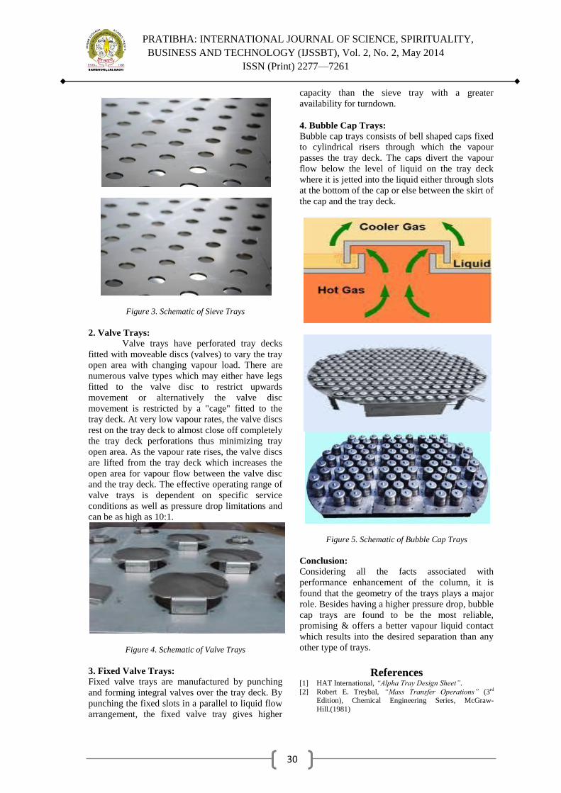
PRATIBHA: INTERNATIONAL JOURNAL OF SCIENCE, SPIRITUALITY,
BUSINESS AND TECHNOLOGY (IJSSBT), Vol. 2, No. 2, May 2014
ISSN (Print) 2277—7261
30
Figure 3. Schematic of Sieve Trays
2. Valve Trays: Valve trays have perforated tray decks
fitted with moveable discs (valves) to vary the tray
open area with changing vapour load. There are
numerous valve types which may either have legs
fitted to the valve disc to restrict upwards
movement or alternatively the valve disc
movement is restricted by a "cage" fitted to the
tray deck. At very low vapour rates, the valve discs
rest on the tray deck to almost close off completely
the tray deck perforations thus minimizing tray
open area. As the vapour rate rises, the valve discs
are lifted from the tray deck which increases the
open area for vapour flow between the valve disc
and the tray deck. The effective operating range of
valve trays is dependent on specific service
conditions as well as pressure drop limitations and
can be as high as 10:1.
Figure 4. Schematic of Valve Trays
3. Fixed Valve Trays:
Fixed valve trays are manufactured by punching
and forming integral valves over the tray deck. By
punching the fixed slots in a parallel to liquid flow
arrangement, the fixed valve tray gives higher
capacity than the sieve tray with a greater
availability for turndown.
4. Bubble Cap Trays:
Bubble cap trays consists of bell shaped caps fixed
to cylindrical risers through which the vapour
passes the tray deck. The caps divert the vapour
flow below the level of liquid on the tray deck
where it is jetted into the liquid either through slots
at the bottom of the cap or else between the skirt of
the cap and the tray deck.
Figure 5. Schematic of Bubble Cap Trays
Conclusion:
Considering all the facts associated with
performance enhancement of the column, it is
found that the geometry of the trays plays a major
role. Besides having a higher pressure drop, bubble
cap trays are found to be the most reliable,
promising & offers a better vapour liquid contact
which results into the desired separation than any
other type of trays.
References [1] HAT International, ―Alpha Tray Design Sheet‖.
[2] Robert E. Treybal, ―Mass Transfer Operations‖ (3rd Edition), Chemical Engineering Series, McGraw-
Hill.(1981)

PRATIBHA: INTERNATIONAL JOURNAL OF SCIENCE, SPIRITUALITY,
BUSINESS AND TECHNOLOGY (IJSSBT), Vol. 2, No. 2, May 2014
ISSN (Print) 2277—7261
31
[3] McCabe, Smith, Harriott et. al., ―Unit Operations of
Chemical Engineering‖ (6th Edition), Chemical
Engineering Series, McGraw-Hill.(2001) [4] Kister, Henry Z, ―Distillation Design‖ (1st Edition),
Chemical Engineering Series, McGraw-Hill.(1992)
[5] Patil N. P., Patil V. S., ―Molecular Sieve Dehydration
Technology for Ethanol Dehydration‖ Chemical Industry
Digest, Page 52-57, September 2012.

PRATIBHA: INTERNATIONAL JOURNAL OF SCIENCE, SPIRITUALITY,
BUSINESS AND TECHNOLOGY (IJSSBT), Vol. 2, No. 2, May 2014
ISSN (Print) 2277—7261
32
Economic Study of Fermentation Kinetics for Production of
Ethanol from damaged Sorghum and Corn grains: a Critical
Review
Sheetal B. Gawande
1, Dr. I. D. Patil
2
1Research Student, SSBT`s, COET, Bambhori, Jalgaon (MS), India
2Professor and Head, Department of Biotechnology, SSBT`s, COET, Bambhori, Jalgaon (MS), India
Abstract
Ethanol production from starchy raw materials
by direct bioconversion is having high potential.
Ethanol production from Corn and sorghum
starch requires the use of amylase and
amyloglucosidase for the pre-treatment starch
before fermentation. Yeast ferments different
sugars at different rates depends on the process
conditions, several factors affect the production
rate of ethanol by fermentation, and thus
through the review of literature in this paper
need to develop a suitable mathematical
description of the fermentation process is
identified. This reveals in interpreting
fermentation measurements for early detection
of poor fermentation performance. The ability
to predict future fermentation behavior,
application to design, advanced control of
fermentation and optimization for economical
ethanol production is possible. Because of rapid
depletion of fossil fuel reserves, alternative
energy sources that are renewable, sustainable,
efficient, cheaper and eco-friendly options.
Keeping this in view, improvements in the
ethanol fermentation have been focused. From
the review of literature it is observed that
kinetic models describing the behavior of
microbiological systems are very useful tool and
it would reduce testing for elimination of
possibilities.
Keywords: Kinetic parameter, mathematical
model, Ethanol, Fermentation, pre-treatment
1. Introduction In recent years, growing attention has been
devoted to the conversion of biomass into fuel
ethanol, considered the cleanest liquid fuel
alternative to fossil fuels. Significant advances
have been made towards the technology of ethanol
fermentation. [1]. Bioethanol is a form of
renewable fuel that can be produced from
agricultural feedstocks such as sugar cane [2],
sorghum [3, 4, 5], organic and food waste (maize)
[6] , banana peel waste [7,8], agro industrial
byproducts [9], starch industy waste [10]. Ethanol
production and fermentation efficiency vary
depending on sorghum variety or crop and the
amount and proportion of sugar in the sweet
sorghum [4]. Sweet sorghum straw has a potential
to be a source for the production of fermentative
sugars that can be subsequently fermented to
ethanol. The conversion of Sweet Sorghum Straw
into fermentative sugars consisted of two steps, the
acid pretreatment followed by enzymatic
saccharification [11]. Simultaneous
Saccharification and Fermentation (SSF) of corn
flour [12], and various lignocellulosic woody
(poplar and eucalyptus) and herbaceous (Sorghum
sp. bagasse, wheat straw and Brassica carinata
residue) materials [13] for ethanol production have
been carried out. An economical bioprocess to
produce the bio-ethanol from soybean molasses at
laboratory, pilot and industrial scales using a strain
of Saccharomyces cerevisiae (LPB-SC) have been
developed[14]. Effect of various carbon sources
such as glucose, fructose and sucrose on growth
kinetics and ethanol productivity of
Saccharomyces cerevisiae PTCC have been
investigated. Growth kinetic parameters with
Malthus, Monod and logistic rate equations have
been determined. The computed maximum specific
growth rates by Monod Growth kinetic model have
been the highest [15]. A non-linear kinetic model
to predict the consumption of different sugars
(glucose, fructose and sucrose) as a substrate,
during an apple wine yeast fermentation with
Saccharomyces cerevisiae strain CCTCC
M201022 have been proposed [16]. The kinetic
parameters of the ethanol fermentation have been
studied by fitting the experimental data with four
different kinetic models, namely Monod, Contois,
modified Monod and Teisser using MATLAB
[17]. Two types of airlift fermenters, conventional
(UT-ALF) and modified (CDT-ALF) have been
investigated to evaluate their performance with
respect to baker‘s yeast growth [18]. Various

PRATIBHA: INTERNATIONAL JOURNAL OF SCIENCE, SPIRITUALITY,
BUSINESS AND TECHNOLOGY (IJSSBT), Vol. 2, No. 2, May 2014
ISSN (Print) 2277—7261
33
concentrations of damaged wheat and sorghum
starch from 10% to 30%W/V were used for
simultaneous saccharification and fermentation to
produce ethanol by utilising crude amylase
preparation from B. subtilis VB2 and an amylolytic
yeast strain S. cerevisiae VSJ4 [19]. Process
optimization for production of sugar bioethanol
from sorghum, a non conventional source of starch
was carried out [20].
2. Mathematical Models There are basic biological models that can be used
to describe biochemical processes successfully.
The experimental data were subjected to different
kinetics models and the model that best fit the
experimental data was adopted. These models are
shown in Table 1.
Table1: Some biological Models Source: [8]
Sr. No. Name Model
1 Logistic Model 𝑦 =
𝑎
1 + exp(𝑏 − 𝑐𝑥)
2 Gompertz model 𝑦 = 𝑎 exp[− exp 𝑏 − 𝑐𝑥 ]
3 Modified Gompertz
model 𝑦 = 𝑎 exp − exp μm exp 1
a 𝜆 − 𝑡 + 1
4 Richards Model 𝑦 = 𝑎 1 + 𝑣. 𝑒𝑥𝑝 𝑘 𝜏 − 𝑥 −
1
𝑣
5 Stannard Model
𝑦 = 𝛼 1 + 𝑒𝑥𝑝 − 1 + 𝑘𝑥
𝑝
−𝑣
6 Schnute Model
𝑦 = 𝑦1𝑏 + 𝑦2
𝑏 − 𝑦1 𝑏
1 − exp −𝑎(𝑡 − 𝜏1)
1 − exp −𝑎(𝜏2 − 𝜏1)
1 𝑏
Logistic model describes the kinetic of glucose
biomass growth and modified Gompertz equation
can successfully describe the kinetics of ethanol
mass concentration with respect to fermentation
time at the experimented temperature [9].
3. Biomass Kinetic Growth Model
A non structured, sigmoidal shaped model,
especially logistic model is widely used to describe
microbial growth. Quite a number of
polysaccharide fermentation processes and
biomass growth have been described by logistic
equation. Under optimal growth condition and
when the inhibitory effects of substrate and
product were neglected, the rate of cell growth
follows the well-known exponential relation as
expressed in equation (1).
𝑑𝑋
𝑑𝑡= 𝑋 𝜇𝑚 ................................... (1)
Where, µm (h-1
) is maximum specific growth rate
of cells in time (t), with respect to the fermentation
conditions, X is biomass concentration (g/l) and; t
is the time.
The equation above means that X increases with
time regardless of substrate availability. In real
life, the given hyperbolic relationship governs the
growth of cell is given by equation (2) below.
𝑑𝑋
𝑑𝑡= 𝜇𝑚 X 1 −
X
Xm ................................... (2)
Where Xmis the maximum biomass concentration
in g.l-1
and, X0 is the minimum or initial biomass
concentration g.l-1
.
This equation is known as the Riccati equation [7]
, using the boundary condition at t=0 then X = X0,
gives a sigmoidal variation of X as a function of
time. Equation (2) can be easily integrated to give
the logistic equation which may represent both an
exponential and a stationary phase. The resulted
equation is shown in equation (3)
𝑋 =𝑋𝑚𝑋0 𝑒𝜇𝑚 𝑡
𝑋𝑚−𝑋0+𝑋0 𝑒𝜇𝑚 𝑡 ................................... (3)
Further simplification gives equation (4) and (5):
𝑋 =𝑋𝑚𝑋0 𝑒𝜇𝑚 𝑡
𝑋𝑚−𝑋0+𝑋0 𝑒𝜇𝑚 𝑡 ................................ (4)
𝑋 = 𝑋
0𝑒𝜇𝑚 𝑡
1−𝑋0𝑋𝑚
1−𝑒𝜇𝑚 𝑡............................... (5)
The equation (5) above is generally known as
logistic equation which can accurately describe the
kinetics biomass growth with time. It may
represent both an exponential and stationary phase,
however, the logistic equation presented above,
does not predict the death phase of microorganisms
after the stationary phase. The use of unstructured
models is completely adequate in those cases
where the substrate concentration is high compared
to the saturation constant in the major part of batch
fermentation. The unstructured model includes the
most fundamental observations concerning

PRATIBHA: INTERNATIONAL JOURNAL OF SCIENCE, SPIRITUALITY,
BUSINESS AND TECHNOLOGY (IJSSBT), Vol. 2, No. 2, May 2014
ISSN (Print) 2277—7261
34
microbial growth processes: (i) the rate of the cell
mass production is proportional to biomass
concentration and (ii) there is an upper (saturation)
limit for growth rate on each substrate [10]
The Monod model is considered the basic equation
of an unstructured model. This model introduced
the concept of growth-controlling (limiting)
substrate, relating the growth rate to the
concentration of a single growth-controlling
substrate [1 = f (S)] via two parameters, the
maximum specific growth rate (µmax), and the
substrate affinity constant (Ks). This model
exhibits the typical hyperbolic shape for growth
rate express in function of substrate concentration.
µ =µ𝑚𝑎𝑥 . 𝑠
𝐾𝑠 + 𝑆
Where, μ is the specific growth rate (h-1
), S is
substrate concentration (g/L), Ks is Monod
constant and μmaxis defined as specific growth rate.
It has been observed that Monod model has a
significant similarity with the Michaelis-Menten
kinetics [11, 12]. Culture that grows on single
substrate can be described by Monod model.
Substrate in Monod model is known as growth-
limiting substrate due to the dominant influence of
a single substrate [11]. Batch fermentation mass
balance for biomass generation rate, substrate
consumption rate and product formation rate can
be illustrated respectively as follows.
𝒅𝑿
𝒅𝒕= µ.𝑿
𝒅𝑺
𝒅𝒕= −
µ.𝑿
𝒀𝒙/𝒔
𝒅𝑷
𝒅𝒕= 𝒒𝒑 𝑿
Where, X is the biomass concentration (g/L);
Yx/sis the biomass yield (g biomass/g glucose); P is
the product concentration (g/L) and qp is the
specific product formation rate (h-1
). The kinetic
parameter such as μmaxwas calculated during the
exponential phase from the slope of the graph of ln
X vs time [12]. Ksvalue is the concentration of
substrate when μis equivalent to half of μmax[11].
The value of Ksis usually small.
Structured models describing culture kinetics
are important in the control of bioreactors, as they
provide a mathematical description of the
mechanism of the process which are required for
optimization and control. The objective of
structured modeling is to obtain expressions that
quantitatively describe the behavior of the process
under consideration. A wide variety of models
have been proposed for the kinetics of the process;
these range from very simple models to more
complex global models, which take into account
the activating and inhibiting effects of the substrate
(glucose and oxygen) and the product (ethanol and
acetic acid). However, none of these studies have
put forward a general model sufficiently well
developed to permit the design of a good simulator
which is capable of performing simulations with
batch process. A developed mathematical model
capable of predicting the cell, substrate, and
ethanol concentrations during the continuous
anaerobic fermentation is necessary. However, it
cannot be expected that any kinetic model will be
directly applicable to a real process situation.
Therefore, mathematical modeling should start
with the simplest type, but it must be reiterated,
modified, and extended until it eventually leads to
an adequate process kinetic model.
4. Ethanol Concentration Model
The modified Gompertz model successfully
described the data of the fermentative production
of ethanol from glucose biomass using a
theremotolerant strain of kluveromyces Maxianus
[9]. The double exponential Gompertz function
Model is written as:
𝑦 = 𝑎 exp[− exp 𝑏 − 𝑐𝑥 ]............. (6)
After modification, modified Gompertz model can
be written as:
𝑦 = 𝑎 exp − exp μm exp 1
a 𝜆 − 𝑡 + 1 ..... (7)
The kinetic parameters are:
y = the ethanol mass concentration (g/L),
𝑎 = the potential maximum ethanol mass
concentration (g/L),
μm = the maximum ethanol production rate
(gl-1
h-1
),
λ = the lag phase or the lag phase or the time
to exponential ethanol Production (h).
t = fermentation time.
Equation (7) can be written as:
𝐴𝐸𝑡𝑜𝐻 = 𝐴𝑚 exp −𝑒𝑥𝑝 𝑃𝑟𝑚 exp 1
𝐴𝑚
𝜆 − 𝑡
+ 1
Where:
𝐴𝐸𝑡𝑜𝐻 = the ethanol mass concentration (g/L),
𝐴𝑚= the potential maximum ethanol mass
concentration (g/L),
𝑃𝑟𝑚=the maximum ethanol production rate (gl-1
h-
1), or productivity
The kinetic parameters of the ethanol mass
concentration of the experimental data were
adopted and subjected to modified Gompertz
model and the result was plotted alongside with the
real life experimental data. Both of the results

PRATIBHA: INTERNATIONAL JOURNAL OF SCIENCE, SPIRITUALITY,
BUSINESS AND TECHNOLOGY (IJSSBT), Vol. 2, No. 2, May 2014
ISSN (Print) 2277—7261
35
show high level significance of correlation with an
R square value of 0.996. The high value of the R
square suggests that the modified Gompertz model
can be successfully used to describe the
fermentation process for the production of ethanol
from glucose biomass.
5. Improvement of the Ethanol Fermentation
Process
5.1 Two-Stage Bioreactor with Recycling for
Continuous Ethanol Production
In order to achieve higher ethanol productivity,
many researchers [12–16] used two or more
bioreactors or packed columns in series with or
without recycling the cells to maintain high
dilution rates. Nishiwaki and Dunn [12–15]
demonstrated a two-stage bioreactor with recycling
the cells by a cell separator at each stage (Fig. 1).
Chaabane et al. [17] studied a two-stage
continuous bioreactor by recycling the cells where
the first reactor was used for cell growth and the
second reactor for ethanol production. Higher
ethanol productivity (up to 41 g L–1
h–1
) was
obtained with complete conversion of glucose to
ethanol in the two-stage system. Bai et al. [18]
observed high fluctuations in fermentation
parameters in three tubular bioreactors arranged in
series (Fig. 2). These fluctuations were attenuated
when the tubular bioreactors were packed with
Intlox ceramic saddle.
Figure1. Two-stage fermenter with cell recycling at each stage [13]
The kinetic parameters were obtained for a
continuous glucose-to-ethanol fermentation with
Saccharomyces cerevisiae in recycling of cells
using the membrane fermenter by Groot [74–77].
For specific growth rate under product inhibition:
𝜇 = 𝜇𝑚 .
𝑆
𝑘𝑠 + 𝑆 1 −
𝑃
𝑃𝑚 𝑛
For specific glucose consumption rate:
𝑞𝑠 = 𝜇𝑚𝑌𝑋 𝑆
For specific ethanol production rate:
𝜐 = 𝑌𝑋 𝑆 𝑞𝑠
where 𝜇is the specific growth rate (h–1
),
𝜇𝑚 . is the maximum specific growth rate (h–1
), S is
the substrate concentration (g L–1
), KS is the
saturation constant (g L–1
), P is the product
concentration (g L–1
), Pm is the maximum product
concentration (g L–1
), qs is the specific
consumption rate of the substrate (g g–1
h), 𝜐is the
specific production rate of ethanol (g g–1
h–1
),
andYx/s is the yield of cells based on the glucose
consumed (g g–1
).

PRATIBHA: INTERNATIONAL JOURNAL OF SCIENCE, SPIRITUALITY,
BUSINESS AND TECHNOLOGY (IJSSBT), Vol. 2, No. 2, May 2014
ISSN (Print) 2277—7261
36
Figure 2 Process diagram for continuous ethanol fermentation using a combined bioreactor system 1, substrate
storage tank; 2, peristaltic pump; 3, stirred tank fermenter; 4, pH controlling unit; 5, temperature controlling unit; 6,
tubular fermenters; 7, thermostat water inlet; 8, thermostat water outlet; 9, broth storage tank; 10, exhaust gas
washing tank; 11, air flow meters; 12, air humidifiers; 13, sampling parts
6. Conclusion
Generally, economic restrictions force industrial
processes to work in a very small range of
operating conditions. Mathematical models are
effective tool for analyzing biological process and
microbial growth phenomenon. The studied model
shows more insight into the environmental
conditions that is surrounding bio-process and can
be used for further development and optimization
of bio-processes. This paper reviews the various
process options and kinetic models adopted
towards resolving the technological challenges to
develop a low-cost commercial process.
Optimization of the cost of ethanol
production is the prime objective of the current
research work. In this direction improvement of
yield and productivity are the major achievements
to reduce the cost of ethanol production per gallon.
Kinetics of biomass production with respect to
time could be illustrated by logistic models.
Kinetics of ethanol mass concentration production
at an operating temperature could be tested by
modified kinetic models. Logistics model could be
well fitted to the experimental data and could be
regarded as sufficient to describe the biomass
production. Also, the modified kinetic model fitted
into the experimental data and could also be
regarded as sufficient to illustrate the fermentation
process for the production of ethanol from glucose
biomass with a novel thermo-tolerant strains
techniques. Experimental and mathematical
modeling, results were compared by several
researchers which shows no significant difference.
Therefore, utilization of mathematical model
would contribute to a better understanding of
effects of various factors affecting the production
of ethanol. In other words, models enable us to
understand, design and control the fermentation
process better and could be also be used for further
process development.
7. Acknowledgment
Authors are thankful to the SSBT`s, College of
Engineering and Technology, Bambhori, Jalgaon
for providing library facility. The authors would
like to thank the staff and colleagues for useful
discussions.
References: [1] K. Manikandan, T. Viruthagiri, Optimization of C/N Ratio
of The Medium and Fermentation Conditions of Ethanol
Production From Tapioca Starch Using Co-Culture of Aspergillus Niger and Sacharomyces Cerevisiea: Intern
J.ChemTech Research 2002. Vol 2, No 2, pg 947.
[2] R.S. Douglas and K. T., Wallenious, The Impact and Benefit of Mathematical Model.(CRC Press, Boca Raton,
FL. 1999)
[3] K. Zajšek, A. Goršek, I. Rogelj, The use of non-structured
models for describing the ethanol production during the
milk fermentation by natural starter cultures 2011
[4] H. Song, S. Jang, J. Park, and S. Lee, Modeling of batch
fermentation kinetics for succinic acid production by

PRATIBHA: INTERNATIONAL JOURNAL OF SCIENCE, SPIRITUALITY,
BUSINESS AND TECHNOLOGY (IJSSBT), Vol. 2, No. 2, May 2014
ISSN (Print) 2277—7261
37
Mannheimia succinici producens, Biochem Eng J, 40(1):
2008, 107–115.
[5] Luong, J., Mulchandani, A. and LeDuy, A., 1988, Kinetics of biopolymer synthesis: a revisit, Enzyme
Microbial Technol., 10(6): 362–332.
[6] F. García-Ochoa, M García-Leó,.and A. Romero, 1990,
Kinetics modeling of xanthan production from sucrose,
Chem Biochem Eng. 35(4) 1990. 15–20.
[7] M.H., Zwietering,., I. Jongenburger, F. Rombouts, and K.
Van‘t Rient, , Modeling of bacteria Growth Curve: Applied and Environmenal Microbiology, Vol. 56, No 6 p
1990. 1875-1881.
[8] Dona, A. C., G. Pages, R.G. Gilbert, M. Gaborieau and P. W. Kuchel, 2009. Kinetics of In Vitro Digestion of
starches Monitored by Time-Resolved 1H Nuclear Magnetic Resonance. Biomacromolecules, 10(3): 638-
644.
[9] Olaoye O.S. and Kolawole O.S. 2013. Modeling Of the
Kinetics of Ethanol Formation from Glucose Biomass in
Batch Culture with a Non Structured Model. International Journal of Engineering Research and Applications
(IJERA) ISSN: 2248-9622 Vol. 3, Issue 4, Jul-Aug 2013,
pp.562-565
[10] M. Tobajas, and E. Garcia-Calvo, ―Comparison of
analysis methods for determination of the kinetic parameters in batch cultures‖. World Journal of
Microbiology & Biotechnology, 16, 2000, pp. 845-851
[11] Doran PM Bioprocess Engineering Principles. London:ACADEMIC PRESS LIMITED, 1997.
[12] Dunn IJ, Heinzle E, Ingham J, Prenosil JE. Biological Reaction Engineering Dynamic Modeling Fundamentals
with Simulation Examples. Second, Completely Revised
Edition. Weinheim: WILEYVCH Verlag GmbH Co. KGaA, 2003.
[13] A. Nishiwaki, I. J. Dunn, Chem. Eng. Commun. 1998, 168 (1), 207. DOI: 10.1080/00986449808912715
[14] A. Nishiwaki, I. J. Dunn, Chem. Eng. Commun. 1997, 162, 179. DOI: 10.1080/00986449708936638
[15] A. Nishiwaki, I. J. Dunn, Biochem. Eng. J. 1999, 4 (1),
37. DOI: 10.1016/S1369-703X(99)00029-7
[16] W. J. Groot et al., Bioprocess Eng. 1992, 8, 39. DOI:
10.1007/BF00369262
[17] F. B. Chaabane et al., Bioprocess Biosyst. Eng. 2006, 29,
49.DOI: 10.1007/s00449-006-0056-1
[18] F. W. Bai, L. J. Chen, W. A. Anderson, M. Moo-Young,
Biotechnol. Bioeng. 2004, 88 (5), 558. DOI:
10.1002/bit.20221

PRATIBHA: INTERNATIONAL JOURNAL OF SCIENCE, SPIRITUALITY,
BUSINESS AND TECHNOLOGY (IJSSBT), Vol. 2, No. 2, May 2014
ISSN (Print) 2277—7261
38
HARMONIC DISTORTION ANALYSIS BY
ARTIFICIAL INTELLIGENCE TECHNIQUE
Bhagat Singh Tomar
1, Bharti Drivedi
2, Anurag Tripathi
3
Research Scholar, Electrical Engg. Department,
Laxmi Devi Institute of Engg. & Technology, Alwar,(Rajasthan),India,1
Professor, Electrical Engg. Department,
Institute Of Engineering and Technology, Luck now (Uttar Pradesh), India2
Associate Professor, Electrical Engg. Department,
Institute Of Engineering and Technology, Luck now (Uttar Pradesh), India3
[email protected],[email protected]
3
Abstract—Harmonic distortion in power
systems is an old problem which continues to
grow in importance due to the proliferation of
non-linear loads and of sensitive electronic
devices. Thus, the need of standards to limit
such distortion is required. Due to the time-
varying nature of the distortion more advanced
techniques are required to properly quantify
their impact.
IndexTerms— non-linear loads, harmonic
distortion, sensitive electronic devices, losses,
sources, resonance, voltage levels, fuzzy logic.
1. INTRODUCTION
Harmonics in electrical power system is
becoming a major concern for electric utility
company and consumers. It is produced by power
electronics and other equipments which are called
non-linear loads. Examples of nonlinear loads are
computers; fluorescent lamp and television in
residential while variable speed drives, inverters
and arc furnaces are mostly common in industrial
areas. Increasing numbers of these loads in
electrical system for the purpose of, such as
improving energy efficiency, has caused an
increase in harmonics pollution. These loads draw
non-sinusoidal current from the system. The
waveform is normally periodic according to supply
frequency which is either 50Hz or 60Hz depending
on the country.
Research, in general, on harmonic distortion aims
at characterizing the distortion, the behavior of the
loads and the power system. Also the effects the
distortion has on loads, the system and the
environment are studied. The research presented in
this thesis concerns the sources of distortion
(loads) and the interaction between those and the
propagation of the distortion in the power system.
Effects on the power system are also studied, e.g.
additional losses, harmonic resonance and related
financial costs. Further, mechanisms affecting the
harmonic active power flow, in a certain point, are
shown. A new mechanism concerning harmonic
current interaction in high voltage transmission
systems, due to a difference in the fundamental
voltage phase angle between two nodes, is
addressed.
2. SOURCES OF HARMONIC DISTORTION
Non-linear equipment or components in the power
system cause distortion of the current and to a
lesser extent of the voltage. These sources of
distortion can be divided in three groups:
a) Loads
b) The power system itself (HVDC, SVC,
Transformers, etc)
c) The generation stage (Synchronous
Generators)
Subdivision can also be made regarding the
connection at different voltage levels. In general,
loads can be considered connected at lower voltage
levels, the power system exists at all voltage levels
and the generation stage at low and medium
voltage levels.
Electronic equipment, supplied from the low
voltage power system, rectifies the ac power to dc
power for internal use at different dc voltage
levels. This is done, either with or without an ac
step down transformer, and a diode rectifier.. The
power range for each device is small, from a few
W up to some kW. The total harmonic distortion,
THD, of the line current is often over 100 % and
consists of all odd multiples of the fundamental
component. In some case the THD can be nearly
150%, mainly depending on the design of the DC-
link and the crest factor of the supply voltage.

PRATIBHA: INTERNATIONAL JOURNAL OF SCIENCE, SPIRITUALITY,
BUSINESS AND TECHNOLOGY (IJSSBT), Vol. 2, No. 2, May 2014
ISSN (Print) 2277—7261
39
Harmonic producing equipments are found in
varied locations from offices to manufacturing
plants and they are becoming inevitable in daily
life. Various harmonic producing equipments are:
(a) Personal computers
(b) Electronic lighting ballasts
(c) Variable and adjustable speed drives
(d) Industrial process controls
(e) Electronic test equipment
(f) Solid state controls
(g) UPS systems
(h) Medical equipment
3. HOW NON-LINEAR LOADS CREATE VOLTAGE
DISTORTION
By far the majority of the voltage distortion found
in today's distribution systems is produced by the
loads themselves, not the supply. Much of today's
electrical load is non-linear, meaning they
consume current in a non-sinusoidal manner.
Since, by definition, a no sinusoidal waveform is
composed of harmonic currents; non -linear loads
are considered to be harmonic current sources. In
other words, by consuming current in a non-
sinusoidal manner, these non-linear loads produce
harmonic currents that circulate through the power
distribution system. Most voltage distortion is the
result of the interaction of these harmonic currents
with the impedance of the electrical distribution
system. As the harmonic currents pass through the
system's impedance, they produce voltage drops at
each harmonic frequency in relation to ohm's Law
- v h = I h x Z h . The voltage drops appear as
harmonic voltages and the accumulation of these
voltages at all the harmonic frequencies produces
the voltage distortion.
The relationship is:
v TH = (v1 ² +v2 ² + v3 ² + v4 ² +...v h ² ) 0.5
(1.1)
where , vTHD =Total harmonic distortion of
voltage.
v h=Voltage at harmonic h.
v1 =Fundamental voltage.
Distortion levels can be quite high when system
impedance is high. A fatal combination is high
densities of non-linear loads in systems with high
impedance or low fault level. This situation is
common when weak sources, such as UPS system
or diesel generators, are used to service electronic
equipment. The problem is magnified further when
the equipment is serviced by long cable runs.
4. SIMULATION
4.1 The Harmonic Distortion Fuzzy Model
The fuzzy model for the harmonic distortion
diagnostic was implemented in MATLAB using
the fuzzy logic toolbox. This toolbox allows for the
creation of input membership functions, fuzzy
control rules, and output membership functions. To
implement this system in Simulink the system will
need to have two different inputs: the harmonic
voltage and the temperature. These two inputs will
then be processed by a fuzzy logic controller that
will output a degree of caution. This degree of
caution is then decoded into one of four possible
outputs: No problem, Caution, Possible Problem,
and Imminent Problem. A simple (two-variable
example) diagnostic system was created as shown
in Figure 1.
Figure 1 Harmonic Distortion Diagnostic Simulink
Model
Figure 2 System Temperature Input

PRATIBHA: INTERNATIONAL JOURNAL OF SCIENCE, SPIRITUALITY,
BUSINESS AND TECHNOLOGY (IJSSBT), Vol. 2, No. 2, May 2014
ISSN (Print) 2277—7261
40
Figure 3 Harmonic Voltage Input
Figure 4 No Problem Output
Figure 5 Caution Output
Figure 6 Possible Problem Output
Figure 7 Imminent Problem Output
Table 1: Membership Rules
If
Harmonic
Voltage is
And the
temperature
is
Then the Output
is
very_low Below normal no _problem
very_low normal no _problem
very_low over_heating no _problem
very_low very_hot caution
low Below_normal no _problem
low normal no _problem
low over_heating caution
low very_hot Possible _problem
medium Below_normal no _problem
medium normal caution
medium over_heating Possible_problem
medium very_hot Possible_problem
high Below_normal caution
high normal Possible_problem
high over_heating Possible_problem
high very_hot Imminent_problem
very_high Below_normal Possible_problem
very_high normal Possible_problem
very_high over_heating Imminent problem
very_high very_hot Imminent_problem
The inputs for this example system have been
shown before; they are randomly generated data
within a valid range. The system can be simulated
using this data. The output signals generated are
shown in Figure 5.3 through Figure 5.6. The
Fundamental and the harmonics will have uniform
random function generators as inputs. These
function generators will generate a uniform
distribution of inputs within the variances . The
total harmonic distortion will be calculated
depending on these inputs and so it will be in the
range of 1% to 13%, these are the best and worst
case scenarios. The temperature variation will
remain the same as in the previous case. Using this
input data and the basic model developed in the
first case a Simulink model can be developed that
processes all the input data and gives an
appropriate indication for each harmonic, the
fundamental, and THD. These indications will
remain the same as in the previous case. Each
indicator will have a fuzzy logic controller that
implements one of three control topologies, one for
the fundamental, THD, and the harmonics. The
final Simulink model can be seen in Figure

PRATIBHA: INTERNATIONAL JOURNAL OF SCIENCE, SPIRITUALITY,
BUSINESS AND TECHNOLOGY (IJSSBT), Vol. 2, No. 2, May 2014
ISSN (Print) 2277—7261
41
Figure 8 Final Simulink Model
4.2 .Results
The inputs for this example system have been
shown before; they are randomly generated data
within a valid range. The system can be simulated
using this data. The output signals generated are
shown in Figure 5.3 through Figure 5.6. The
Fundamental and the harmonics will have uniform
random function generators as inputs. These
function generators will generate a uniform
distribution of inputs within the variances given in
Table 2. The total harmonic distortion will be
calculated depending on these inputs and so it will
be in the range of 1% to 13%, these are the best
and worst case scenarios. The temperature
variation will remain the same as in the previous
case. Using this input data and the basic model
developed in the first case a Simulink model can
be developed that processes all the input data and
gives an appropriate indication for each harmonic,
the fundamental, and THD. These indications will
remain the same as in the previous case. Each
indicator will have a fuzzy logic controller that
implements one of three control topologies, one for
the fundamental, THD, and the harmonics. The
final Simulink model can be seen in Figure.
Figure.9 All System Inputs (top down): Fundamental,
Third, Fifth, Seventh Harmonics and Temperature
Figure 10 Output Indicators (Top down): Fundamental,
Third, Fifth, Seventh Harmonics and THD.

PRATIBHA: INTERNATIONAL JOURNAL OF SCIENCE, SPIRITUALITY,
BUSINESS AND TECHNOLOGY (IJSSBT), Vol. 2, No. 2, May 2014
ISSN (Print) 2277—7261
42
5. CONCLUSION
The conclusions are that non-linear loads generate
current distortion up to 200 % THD. The tendency
for modern loads is a reduction of the lower order
harmonics, below 1 kHz, and an increase of higher
frequency components, up to 100 kHz. The current
distortion decreases at higher voltage levels,
around 5 % THD, mainly due to mixing with
passive loads but also due to current interaction
between single and three phase non-linear loads.
The voltage distortion is also highest at low
voltage levels, mostly below 6 % THD, and
decreases down below 2 % at higher voltage
levels. A dominating source of distortion, at all
public voltage levels, is the use of television
receivers at evening time with dominating 5:th and
7:th harmonics, up to 0.5 % of the fundamental
component at 132 kV and 400 kV levels.
In this study harmonics modeling of office
equipments is realized for harmonic analysis of
modeled systems in Simulink with the help of
measured real data, voltage-current values and
harmonic current spectrums; proposed Simulink
nonlinear resistance model and harmonics current
injection model. According to Fig.6 and Fig.7 line
current values acquired from nonlinear circuit
(time domain) and harmonic current injection
circuit (frequency domain) are very close and
better than expected tolerances (<%0.1)
THD value of neutral current observed from Fig.7
and Fig. 8 is greater than %200, thus some
harmonic mitigation options, such as oversizing
conductors (especially neutral in three-phase
circuits with shared neutrals), applying passive or
active harmonic filters, must be carried out and
detailed neutral harmonic analysis is needed for
circuits mainly consisting of office equipments.
REFERENCES
[1] J. Arrillaga, D.A. Bradley, P.S. Bodger, Power System
Harmonics, John Wiley & Sons Ltd., 1985.
[2] J. Arrillaga, B. C. Smith, N. R. Watson, A. R. Wood,
Power System Harmonics, John Wiley & Sons Ltd., 1997.
[3] G.T. Heydt, Electric Power Quality, Stars in a Circle
Publications, 1991. [4] R. C. Dugan, M. F. McGranaghan, H. W. Beaty,
Electrical Power Systems Quality, McGraw-Hill, 1996.
[5] A. Mansoor, E.R. Collins, M.H.J. Bollen, Sylvain Lahaie,―Behaviour of Adjustable-Speed Drives during
Phase Angle Jumps and Unbalanced Sags‖, PQA ´97
Europe, June 15-18, 1997. [6] [6] A. Emanuel, ―Apparent power: Components and
Physical Interpretation‖, ICHQP ‗98, Athens, Greece,
October 14-16, 1998. [7] S-L. Lu, C.E. Lin, C-L. Huang, ―Injected Harmonic
Losses Analysis and Estimation due to a 12-pulse AC-
DC Converter Load, Int. Conf. On Industrial Electronics,
New Orleans, LA, Nov 1997.
[8] A.Tugulea,―Power in Distorted Electromagnetic Fields‖, ICHQP ‗98, Athens, Greece, October 14-16, 1998.
[9] J. Lundquist, ―Field Measurements of Harmonic
Distortion and the Role of the DC-Link Inductor‖, ICHQP ‗98, Athens, Greece, October 14-16, 1998.
[10] M.H.J. Bollen, Understanding power quality
problems:voltage sags and interruptions, New York: IEEE Press, 1999.
[11] R. Gretsch, Ch. Kuschnarew, ―Interaction of Active
Compensation and Rectifier Loads‖, CIRED ‘97, 2-5 June, 1997.
[12] H. Seljeseth, et.al, ―Voltage Transformer Frequency
Response. Measuring Harmonics in Norwegian 300 kV and 132 kV Power Systems‖, ICHQP ‗98, Athens,
Greece, October 14-16, 1998.
[13] H. Stoltz, ―Kartläggning elkvaliteten påsvenska
kraftnätet‖, Examensrapport, EKC, KTH, 1995.
[14] Elforsk rapport, 97:3, ―Begränsning vertoneri elnätinom
tätort‖, Elforsk, January 1997.
[15] A. Mansoor, ―Low Order Harmonic Cancellation:
Impactof Low-Voltage Network Topology‖, IEEE PES
Winter Meeting, 1999.

PRATIBHA: INTERNATIONAL JOURNAL OF SCIENCE, SPIRITUALITY,
BUSINESS AND TECHNOLOGY (IJSSBT), Vol. 2, No. 2, May 2014
ISSN (Print) 2277—7261
43
Extracting Trustworthy Data from Multiple Conflicting
Information using Semi-Supervised Approach
Priti R. Sharma1, Manoj E. Patil
2,
1ME (CSE),SSBT‘s,COET Bambhori,Jalgaon,[email protected], India;
2Deptt of ComputerEngineering, SSBT‘s, COET Bambhori, Jalgaon, [email protected], India;
Abstract –At the end of the last century the
appearance of the World Wide Web (WWW)
led to a rapid growth in the Internet and in the
quantity of accessible information for users.
The information that has accumulated on
WWW represents huge knowledge base that
may prove useful for various applications. Now
day people depend on the Webfor
everything.But information retrieved is not
guaranteed trustworthy, not always trustable.
Truthfinder is used to find trustworthy data
using unsupervised approach. It is assumed that
a fact provided by more sources is more likely
to be correct. The proposed system based on the
semi supervised approach. This uses some
training data which will help for improving
performance. Experimental analysis shows that
the proposed algorithm is more effective than
unsupervised approach and which help to
resolve veracity problem.
Keywords:Truth discovery, semi supervised;
I INTRODUCTION
The World Wide Web has become a necessary part
of our lives and might have become the most
important information source for most people.
Every day, people retrieve all kinds of information
from the Web. For example, when shopping
online, people visit websites concerned with
required product and find product specifications.
When they want to know the answer to a certain
question, they go to Ask.com and google.com.
Now days for getting updates, reading newspeople
always take the help of websites. e.g. ifperson want
to get the knowledge of ‗C‘ language then also
website play very important role.―Is the World
Wide Web always trustable?‖ Unfortunately, the
answer is ―no.‖ There is no guarantee for the
correctness of information on the Web. As website
use is most popular then data copying on web also
popular.Conflicting information present on web is
the common thing now days. Usercannot get the
relevant accuratedata most of the time. More
problems has to face in searching data for facts
changing with time, since out-of-date information
often exists in more web sites than up-to-date
information[9].
A new problem called the Veracity
problem is recognized now a days, which is
formulated as follows: Given a large amount of
conflicting information about many objects, which
is provided by multiple websites (or other types of
information providers), how to discover the true
fact about each object[1].The trustworthiness
problem of the web. According to a survey on
credibility of web sites[1]:1.54% of Internet users
trust news web sites most of time.2.26% for web
sites that sell products.3.12% for blogs
Existing system tried to resolve this problem with
unsupervised approach. TruthFinder is used to
resolve veracity problem. Truthfinder is used to get
the true facts from conflicting information .But
better solution is to go for some kind for
supervision.i.e. result can be improved when we
use semi supervise approach instead of
unsupervised approach. Proposed system is based
on semi supervised approach. We come to
recognize that the even a small amount of training
data also greatly help for improving the
performance [9].
The remainder of the paper is organized
as follows.The next section discusses the related
work. Section III takes the overlook on existing
system. In section IV, proposed system is
discussed along with algorithm and UML
diagrams. Section V gives the experimental
analysis. Lastly conclude discussion in section VI.
II Related Work
Quality assessment is important is information
retrieval.The research on Ranking algorithm is
going on from many years. Some researchers used
link analysis I their ranking algorithms. The
popularity of link analysis and the assumptions
about its role in search engine rankings has led to
great efforts by search engines optimization
professionals[3, 6]. Many links are set only to gain
influence on the ranking of certain pages. The
objective of these approaches is to ground the
quality evaluation on a broader knowledge base.
Not only the pages often cited by web page authors
but also pages often visited should be regarded as
being of high quality. The most popular algorithm
is PageRank. The basic assumptionof PageRank
and similar approaches is that the number of in- or
back-links of a Web page can be used as a measure

PRATIBHA: INTERNATIONAL JOURNAL OF SCIENCE, SPIRITUALITY,
BUSINESS AND TECHNOLOGY (IJSSBT), Vol. 2, No. 2, May 2014
ISSN (Print) 2277—7261
44
for the popularity and accordingly for the quality
of a page[5].PageRank assigns an authority value
to each Web page which is primarily a function of
its back links. Additionally, it assumes that links
from pages with high authority should be weighed
higher and should result in a higher authority for
the receiving page. The algorithm is carried out
iteratively until the result. However, link analysis
has several serious shortcomings. The number of
in-links for Web pages follows a power law
distribution. In such a distribution, the median
value is much lower than the average. This means,
that many pages have few in-links while few pages
have an extremely high number of in-links. This
finding indicates that Web page authors choose the
Web sites they link to without a thorough
qualityevaluation. The PageRank technique,
introduced by Page et al. [8], actually tried to mend
this problem by looking at the importance of a
page in a recursive manner: ―a page with high
PageRank is a page referenced by many pages with
high PageRank‖. Drawback of pageranking: Any
website having higher visits will be having higher
pagerank irrespective of the content in data, so
there will be problem if website having higher
pagerank and giving wrong data, many user will
get confused or blindly believe conflicting or
wrong data from other website. Page ranking is use
to find pages with high authorities. The user
predicts the true information according to the
ranking of page.
Finally comment is that it is not true that
most popular website will provide the true fact.
This assumption is totally wrong because out of
date information is remain present on many
websites.Hubs and Authorities (Kleinberg, 1999)
gives each page a hub score and an authority score,
where its hub score is the sum of the authority of
linked pages and its authority is the sum of the hub
scores of pages linking to it[2].After that the HITS
algorithm is proposed by Kleinberg in 1988. HITS
algorithm identifies two different forms of Web
pages called hubs and authorities. Authorities are
pages having important contents. Hubs are pages
that act as resource lists, guiding users to
authorities. Thus, a good hub page for a subject
points to many authoritative pages on that content,
and a good authority page is pointed by many good
hub pages on the same subject. HITS algorithm is
ranking the web page by using in-links and out-
links of the web pages. The veracity problem i.e.
the conformity of truth is not resolved in above
algorithm. Research work was to find trustworthy
data. Voting is the easiest way of computing the
best fact related to an object is to choose the one
with maximum number of votes. This method,
however, does not provide good result.Yin, Han
[7] first propose Truthfinder algorithm to find true
facts. TruthFinder studies the interaction between
website and the facts they provide and infer the
trustworthiness of websites and confidence of fact
from each other.
III Existing System
3.1 Unsupervised Approach:
Existing System uses unsupervised
approach to resolve veracity problem. The first
algorithm proposed to find true fact from false fact
is TruthFinder which is unsupervised[7]. It is
assumed that a fact providedby more sources
(especially more trustworthy and more
independentsources) is more likely to be correct.
They all use iterativeapproaches, which start by
assigning the same trustworthiness toall data
sources, and iterate by computing the confidence
of eachfact and propagating back to the data
sources. The input of TruthFinder is a large
number of facts in a domain that are provided by
many websites specified in fig 1. There are five
facts related to two objects. These five facts are
from different four websites. There are usually
multiple conflicting facts from different websites
for each object, and the goal of TRUTHFINDER is
to identify the true fact among them.
Fig1: Facts, Objects and Information Providers
(Websites) [7].
3.2 Drawbacks of Truthfinder:
Truthfinder makes some assumptions.
Usually there is only one true fact for a property of
an object.This true fact appears to be the same or
similar ondifferent websites. It is assumed that an
object isassociated with only one type of fact.
The above assumption does not true every time.
Accuracy depends on these assumptions [7].
Drawback:
W1
O1
O2
f5
f4
f3
f2
f1
W4
W3
W2
Websites Facts Objects

PRATIBHA: INTERNATIONAL JOURNAL OF SCIENCE, SPIRITUALITY,
BUSINESS AND TECHNOLOGY (IJSSBT), Vol. 2, No. 2, May 2014
ISSN (Print) 2277—7261
45
It is assumed that a provider either providesgood
facts for every object or bad facts for everyobject.
It is assumed that there is onlyone true value for an
object. But often, multiple values(set) could be true
sometimes with different degrees oftruth. It is
assumed that number of providers providing the
true facts are much more than the numberof
providers providing the bad fact [11].
IVProposed System:
We can say that since TruthFinder is unsupervised
approach there is some problem in finding true
facts.Some level of supervision can help the
iterative fact finding algorithm in right
direction.Soit is better solution to go for
semisupervised approach.
The approach is based on three principles:
(i) facts provided by the same data source should
have similar confidence scores, (ii) similar (and
therefore mutually supportive) facts should have
similar confidence scores and (iii) if two facts are
conflicting, they cannot be both true [9].
4.1System overview architecture:
Fig. 2 shows the system overview architecture.
User has to enter the keyword he want to search
and then it is processed to find the trustworthy
information through semisupervised truthfinder.
Fig 2: System overview architecture
SemisupervisedTruthfinder Algorithm:
1. Start
2. Take input i.e. search table, ground truth
fact, nskeywords& additional keywords
3. If (search == normal search)
Then List of sites by nskeyword.
4. else if( search == semisupervised search)
Then list sites in descending order by
confidence score.
5. Select url from search and fact table
6. If (url_search_table == url_fact_table)
Then Update confidence scoredocheck
nscount and display url across that greater
countwhile(confidence score == 1)
7. Subsequently arrange url in descending
order according to confidence score 0 and -
1.
8. Stop.
In semisupervised TruthFinder, a confidence score
is assigned to each fact, so that true facts have
higher scores than false facts [9] Ground data are
used to retrieve query result from Data Source.We
maintain the ground truth data which contain set of
websites.In normal search all related websites are
listed without any priority.
In semi supervised search, we have to
provide additional key words with the normal
search keyword. The ranked websites are listed
after comparing with the ground truth fact data
set. Ground truth data contain a small set of highly
confident fact and use them to infer the
trustworthiness of data sources and confidence of
facts.
For semisupervised search, the confidence
score will be calculated by the site visited by the
user. Comparing with the ground truth sites, if the
visited site is same as the ground truth fact site it'll
be consider as true fact site and its value is 1. if it
is not same then it'll be considered as false facts
site and its value is -1. If the user doesnot visit the
site it'll be taken as unknown site and its value is 0.
4.2 UML Diagrams of System:
Use case diagram:
It shows the interaction between use cases &
actors. Fig 3 shows use case diagram of system.
Two actors normal_search &
semisupervised_search initiates the number of use
cases e.g read keyword, load database, listing from
search table are perfomed by normal_search.
Whereas read url from search table, check
confidence score of url, check nscount of url,
display url in descending order, update confidence
score and nscount are perfomed by
semisupervised search.
Query
formation
Search
type
Conflict data and
untrustworthy
data
Normal
search
Semisupervised
Search
SemisupervisedTruthFin
der and trustworthy
data finding
Input
Keyword
Search result (Untrustworthy data)
Search result
(Trustworthy
data)

PRATIBHA: INTERNATIONAL JOURNAL OF SCIENCE, SPIRITUALITY,
BUSINESS AND TECHNOLOGY (IJSSBT), Vol. 2, No. 2, May 2014
ISSN (Print) 2277—7261
46
Fig 3:Use case diagram
Class Diagram:
It shows the interaction between classes in the
system. Search class has attributes - search type
and nsurl. Operations – geturl(), displayurl() are
also used in child class normal_search and
semisupervised_search. Fig 4 shows class
diagramof system.
Fig 4: Class diagram
State diagram:
It provides way to model the various states in
which an object can exist. Fig 5 shows state
diagram of system. State diagram is drawn for
semisupervised search. Fig shows more dynamic
behavior of system.
Fig 5: State diagram
Sequence diagram:It is used to show the flow of
functionality.Fig 6 shows sequence diagram of
system. It shows the flow of sequence of
semisupervised search. How search query is
processed.
Fig 6: sequence diagram
List url from search tablenormal_search
Read keyword
Load database
Read url from search table
match keyword from fact table
Check confidence score of url
Check nscount of url
Display url in descending order
Update confidencescore& nscount
semisupervised_
search
select search type
semisupervised search
read url from search table
normal search
match keyword from fact table
check confidence score of url
check nscount of url
display url in dscending order
update confidencescore & nscount
o:semisupervis
ed search : semisupervised
_search
search query search database
& fact database
outputhome
enter keyword
valid keyword
search url
result page
return

PRATIBHA: INTERNATIONAL JOURNAL OF SCIENCE, SPIRITUALITY,
BUSINESS AND TECHNOLOGY (IJSSBT), Vol. 2, No. 2, May 2014
ISSN (Print) 2277—7261
47
Collaboration diagram:
It shows exactly the same information as the
sequence diagram. However the collaboration
diagram shows this information in a different way.
. Fig 6 shows sequence diagram of system
Fig 7: Collaboration diagram
V Experimental analysis:
In previous work [9], real world data set containing
authors of computer science books is considered.
Same data set is used in [1], [7]. We take the very
small data set of different types. Our data set
contains 500 websites. We include the different
keywords in our experiment such as book author,
weather, directors of films etc.
nsid
nsurl
nscount
confidencescore
32 http://www.accuweather.com/en/in/india-weather
1 -1
33 http://in.weather.yahoo.com/
0 0
34 http://www.weather-forecast.com/countries/India
0 0
35 http://www.timeanddate.com/weather/india
1 -1
36 http://www.bbc.co.uk/weather/1269750
0 0
37 http://www.mapsofindia.com/weather/
0 0
38 http://in.weather.com/national
3 1
39 http://www.imd.gov.in/
2 -1
Table1: search table for query ‗weather india‘
Fact id url keyword1 keyword2
4 http://www.imd.gov.in/ weather india weather report india
5 http://in.weather.com/national weather report india weather india
Table2: fact table for keyword ‗weather india‘
First ground truth training database is used. The
confidence score of the ground truth facts is
manually set to 1 indicating that these websites are
trustworthy [9]. The confidence score of website of
false fact is set to -1.Additional keywords are used
for semisupervised search. Semisupervised
: semisupervised
_search
search
queryo:semisupervi
sed search
search database
& fact database
output
home
2: valid keyword
3: search url
4: result page
5: return
1: enter keyword

PRATIBHA: INTERNATIONAL JOURNAL OF SCIENCE, SPIRITUALITY,
BUSINESS AND TECHNOLOGY (IJSSBT), Vol. 2, No. 2, May 2014
ISSN (Print) 2277—7261
48
Truthfinder list the url on the basis of confidence
score and nscount. The result of semisupervised
search for keyword ‗weather india‘ is computed on
the basis of confidence score and nscount.
Conclusion:
In this system, semisupervised approach is used.
After analysis, it is observed that there is a big
difference in normal search and semisupervised
approach of TruthFinder.Since ground truth data is
present, it helps to improve the performance of
finding true facts from websites.
References [1] Xiaoxin Yin, Jiawei Han, Philip S. Yu,‖ Truth Discovery
with Multiple Conflicting Information Providers on the Web‖ San Jose, California, USA KDD‘07, August 12–
15, 2007
[2] Jeff Pasternack Dan Roth, ―Knowing What to Believe (when you already know something).‖ Proceedings of the
23rd International Conference on Computational
Linguistics (Coling 2010), pages 877–885, Beijing,
August 2010
[3] Jiawei Han, ―Mining Heterogeneous Information Networks by Exploring the Power of Links.‖Springer-
Verlag Berlin Heidelberg 2009
[4] Jiawei Han and MichelineKamber, ―Data Mining: Concepts and Techniques.‖
[5] LiseGetoor ,―Link Mining: A New Data Mining
Challenge‖, SIGKDD Explorations. Volume 4, Issue 2 - page 1
[6] T.Mandl, Implementation and Evaluation of a Quality-
Based Search Engine, proc. 17th ACM conference hypertext and hypermedia, 2006.
[7] Xiaoxin Yin, Jiawei Han, Philip S. Yu, ―Truth Discovery
with Multiple ConflictingInformation Providers on the Web‖, IEEE transactions on knowledge and data
engineering, vol. 20, no. 6, June 2008
[8] Ricardo Baeza-
Yates,PaoloBoldi,CarlosCastillo,―Generalizing PageRank:
Damping Functions for Link-Based Ranking Algorithms‖,
SIGIR‘06, August 6–11, 2006, Seattle, Washington, USA. [9] Xiaoxin Yin, Wenzhao Tan‖ Semi-Supervised Truth
Discovery‖ WWW 2011, March 28–April 1, 2011,
Hyderabad, India.ACM 978-1-4503-0632-4/11/03. [10] R.Guha, Ravi Kumar, Andrew Tomkins, ―Propagation of
Trust and Distrust‖, ACM 158113844X/04/0005.

PRATIBHA: INTERNATIONAL JOURNAL OF SCIENCE, SPIRITUALITY,
BUSINESS AND TECHNOLOGY (IJSSBT), Vol. 2, No. 2, May 2014
ISSN (Print) 2277—7261
49
Experimental Investigation of Backpressure Variation on a
Single Cylinder C. I. Engine System Performance
Prashant P. Bornare1,
1M.E. student, SGDCOE, Jalgaon, MS, India
Dr. D. S. Deshmukh2
2Professor & Head, Department of Mechanical Engineering, S.S.B.T.‘s, C.O.E.T., Bambhori, Jalgaon
Prof. R.Y. Patil3,
3H.O.D. Mechanical, SGDCOE, Jalgaon, MS, India Jalgaon, (M. S.), India
Abstract— Research paper concentrates on
backpressure phenomenon in case of
compression ignition engines. Effective after
treatment techniques utilization specifically for
C.I. engines, requires critical analysis of the
complete exhaust system employed. Search on
After Treatment Devices as a modern
technology is very active because particulate
matter is designated as a major cancer material.
Regeneration phenomenon in After Treatment
Device is a subject of special interest for design
and development of Particulate Matter emission
control activities. The Backpressure acting on
engine is most important factor which basically
deteriorates the engine and emission control
performance. In the present work, critical study
of backpressure rise which is undesired for
system performance view point and
experimental study of the effect of back
pressure generated on the C.I. engine, with and
without the use of a specially designed After
Treatment Device is done. To minimize the
problem of back pressure rise because of after
treatment techniques applications, some
remedial actions are also suggested.
Keywords— After Treatment Device,
Backpressure, Exhaust Emissions, After Treatment
Device, Compression Ignition engine.
1) INTRODUCTION
The exhaust system routes exhaust gas
from the engine and exhaust it into the
environment, while providing noise attenuation
and after treatment of the exhaust gas to reduce
emissions. One of the most important sources of
vehicle noise, the noise associated with exhausting
combustion gases from the engine, is controlled
using mufflers. A number of sound reduction
techniques are employed in mufflers, including
reactive silencing, resistive silencing, absorptive
silencing, and shell damping. Exhaust gas
properties which are important for the exhaust
system design include its physical properties;
exhaust gas temperature which depends on the
vehicle duty and the exhaust gas flow rate. The
most important of these engine technologies are
advanced fuel injection systems, air intake
improvements, combustion chamber modifications,
and electronic engine control. Additionally,
exhaust gas recirculation (EGR) was introduced on
both light- and heavy-duty diesel engines to
control NOx emissions. Exhaust emission from
automobiles can be controlled in three different
ways. One is to promote more complete
combustion, so that there is less byproduct. The
second is to reintroduce excessive hydrocarbons
back into the engine for combustion, and the third
one is to provide an additional area for oxidation or
combustion to occur. Thus the after treatment
techniques seem to be more feasible as compared
to other alternative techniques for reducing exhaust
emissions instead of going for engine and fuel
modifications. Engine After treatment requirement
changes in response to changing Pollution control
norms or legislation, which usually requires new
technologies to be introduced. Low emission
engine design-combined with increased exhaust
gas after treatment will continue to play important
role in future diesel engines.
2) DIESEL EXHAUST EMISSIONS
Overview of the regulated and unregulated diesel
exhaust emissions is discussed here.
It includes the regulated gaseous diesel emissions
nitrogen oxides, hydrocarbons and carbon
monoxide and some of the non-regulated
emissions including sulfur dioxide and nitrous
oxide. Diesel particulate matter is the most
complex of diesel emissions. Diesel particulates, as
defined by most emission standards, are sampled
from diluted and cooled exhaust gases. This
definition includes both solids, as well as liquid

PRATIBHA: INTERNATIONAL JOURNAL OF SCIENCE, SPIRITUALITY,
BUSINESS AND TECHNOLOGY (IJSSBT), Vol. 2, No. 2, May 2014
ISSN (Print) 2277—7261
50
material which condense during the dilution
process.
3) EXHAUST AFTER TREATMENT
SYSTEM DESIGN CRITERIA:-
Engine After treatment requirement changes in
response to changing Pollution control norms or
legislation, which usually requires new
technologies to be introduced. New technologies
place particular challenges on after treatment
systems. A brief overview is given here, the main
trends in after treatment system development have
been, 1) A requirement for reduced backpressure
in all types of C.I. engines in old, present & future
engines using diesel or any alternate renewable
fuel. Backpressure rise causes increase in fuel
consumption. 2) A requirement for efficient
exhaust energy recovery system and new improved
Noble & Non-noble metal based economical
catalyst technologies, to obtain maximum possible
conversion efficiency for pollution control with
durability issues.
4) BACKPRESSURE MINIMIZATION
The prime objective for design engineers is to
obtainminimumbackpressure with durability. Each
alternation in after treatment system or exhaust
system causes variations in backpressure on C.I.
engine. But after successful design also
backpressure on a particular engine increases
during its use because of following reasons –
A. Engine Design, Fuel and Lubrication Oil
Modifications: In most of the C.I. engine
applications lack of space availability needs
compactness of after treatment devices, it creates
restriction in exhaust flow. Exhaust flow area from
engine exhaust valve or port near exhaust manifold
should be critically analyzed and designed.
Precautions should be taken during the design of
complete exhaust system such that the
backpressure just at the exhaust port or valve
region must not increase. This requires extra
volumes near exhaust valve or port for stabilization
of exhaust flow. During exhaust process, engine
cylinder works as convergent part, port or valve
flow area as throat and manifold as divergent part,
for nozzle like operation. This section must be
designed for maximum mass flow rate and energy
equation should be used for obtaining the
minimum pressure at throat section so as to utilize
maximum exhaust energy with specific objective
of minimum possible back pressure on engine
cylinder.
To ensure that lubricants provide all of the
lubricating oil functions required in modern
engines, a number of oil specifications have been
developed in the USA, EU and Japan. One of the
main drivers in the development of oil
formulations for diesel engines with exhaust after
treatment is the reduction of sulfated ash,
phosphorous and sulfur. Highest performance from
engine system requires unique engine design &
after treatment system for optimal fuel energy
conversion.
B. After Treatment System Modifications: Diesel after treatment strategies may include
muffler, After Treatment Device or Catalytic
Converter, Thermal reactor, Turbocharger, EGR
system, etc., in the exhaust system for heat
recovery & emission control activities. ATDs are
designed to trap diesel particulate matter (PM) to
achieve a net decrease in PM emissions. The
device captures ash, but the accumulation of ash in
the device is sufficient to cause a rise in back
pressure. In practice, these devices will also need
to regenerate quickly and relatively cheaply when
they become blocked. The device can be fitted to
both new and old engines. The failure of catalyst
may be due to System component meltdown,
Carbon deposit, Catalyst fracture, Deactivation of
diesel catalyst etc. Improper regeneration or after
treatment device component failure may cause
Backpressure rise, mostly it happens because
Particulate matter consists of noncombustible
compounds, so 100% regeneration is not possible.
To address this concern, Considering
automobile power plant as a complete system, it is
a complex system made up of several other equally
complex sub-systems, each is distinct from the
others but they all share some common features
and goals that allow them to work together.
Backpressure reduction procedure requires that
ATDs be installed with backpressure monitors that
will alert the operator when the backpressure
exceeds some pre-set level. With some insight into
the state of the ATD, the operator can avoid
potentially costly failures. Even when regenerating
properly, adding a ATD to the exhaust system of a
vehicle will increase the backpressure by some
amount. If more work is required from the engine
to push combusted gases out through the exhaust
system, a fuel economy penalty results. Even
though the backpressure caused by ATD is within
the engine manufacturer‘s specified limits, it is
noted in the test data that even a little bit of rise in
backpressure show fuel economy penalty. Some
active systems may collect and store diesel PM
over the course of a full day or shift and can be
regenerated at the end of the day or shift with the
vehicle or equipment shut off. A number of the
filters used in stationary like applications operator
or driver can be trained to remove and regenerate

PRATIBHA: INTERNATIONAL JOURNAL OF SCIENCE, SPIRITUALITY,
BUSINESS AND TECHNOLOGY (IJSSBT), Vol. 2, No. 2, May 2014
ISSN (Print) 2277—7261
51
externally at a ―regeneration station‖ for achieving
complete regeneration with ease. Because they can
have control over their regeneration and may not
be much dependent on the heat carried in the
exhaust.
5) EXPERIMENTAL SETUP
The engine used for experimentation has following
specifications
1. Make: Kirlosker, single cylinder, four stroke
compression ignition engine.
2. Rated power output: 5 H.P
3. Speed: 1500 R.P.M.
4. Stroke length: 110 mm
5. Bore diameter: 80mm
6. Loading type: Water resistance type load,
with copper element and load changing
arrangement
7. Moment arm: 0.2 meter
8. Orifice diameter (for air box): 25mm
9. Co-efficient of discharge of orifice: 0.64
Figure: 1 Schematic view of experimental set up.
6) After Treatment Device (ATD):
1) Space velocity: 50,000 hr-1
2) Catalyst used: copper based catalyst system
3) Circular perforated copper plates with 256 no.
of holes per square cm and copper rings made
up of 5 mm diameter rod.
4) Flange arrangement for dismantling and
varying no. of perforated plates and no. of
rings, more details are given in figures.
Figure: 2 View of After Treatment Device with copper plates
7) EXPERIMENTATION WORK
Development of practically feasible after
treatment device can be considered as one of the
most challenging tasks related to the after
treatment technologies. But owing to the
drawbacks in after treatment technique that even a
small rise in back pressure adversely affects the
5 15 15 30
15 FLOW
DIRECTION
FLANGE TYPE ARRANGEMENT
ALL DIMENTIONS ARE IN CM

PRATIBHA: INTERNATIONAL JOURNAL OF SCIENCE, SPIRITUALITY,
BUSINESS AND TECHNOLOGY (IJSSBT), Vol. 2, No. 2, May 2014
ISSN (Print) 2277—7261
52
system objectives and high cost involved with it,
these are uneconomical. Hence in present work an
attempt is made to use perforated circular copper
plate arrangement in After Treatment Device.
Throughout the complete trials conducted, the
speed of the engine is kept constant, at 1500 rpm
and also engine jacket cooling water is kept
constant at 0.1666 liters/sec, so as to provide ease
in comparison of different parameters, in some
cases by varying the load on the engine also.
Further during the trials on ATD, each times the
perforated plates and rings were cleaned by water
and then by carbon tetra-chloride solution. While
changing the number of plates and rings i.e. every
times the fresh copper plates and rings were used.
To reduce the backpressure on the engine,
maximum no. of plates (i.e. 20 plates) provided
with extra 8 no. of holes, of 5 mm diameter were
used for determining the effect i.e. back pressure
reduction mainly. The different parameters are
compared with the values of same parameters
without using ATD, for the same engine output
conditions.
8) RESULTS AND DISCUSSIONS
1) Backpressure is observed to be directly
proportional to the number of plates used
obviously because of increase in resistance to
exhaust gas flow, at the same engine operating
conditions. After Treatment Device is designed to
achieve nozzle like operation to reduce exhaust
back pressure, which shows potential remedial
technique.
2) Fuel consumption is also observed to be directly
proportional to the back pressure on the engine, at
the same operating conditions. The desire for
countries and automotive manufacturers to reduce
emissions includes CO2 emissions that arise from
burning fuel in engines. There is a direct
correlation between a vehicle‘s fuel consumption
and the CO2 emitted from that vehicle.
3) Effect of increased backpressure on engine
performance: - Exhaust system components are a
source of engine exhaust back pressure. An
increased back pressure level causes increase in the
pumping work requirement and hence it increases
the specific fuel consumption thereby increased
emissions and negatively affects engine
performance.
4) Effect of increased backpressure on conversion
efficiency of ATD: - Though it appears to be the
same conversion efficiency of the ATD, the
emissions actually at the exit are very high because
of the increase in backpressure fuel consumption
increases which ultimately increases the amount of
pollutants at the feed stream of the ATD.
Variations in exhaust emissions are compared at no
load condition, using different no. of plates the
conversions obtained are (NOx -18.05 %, HC -56
%, C0 -8.33% and smoke density -11.11%)
maximum using 8 no. of plates arrangement.
Performance Characteristics (at constant 1500 rpm)
Graph-1 Variation in Fuel consumption and no. of plates Vs back pressure,
using ATD with different no. of plates arrangement
0
5
10
15
20
25
30
35
Back pressure in cm of H2O
Fu
el
rate
in
kg
/hr
No. of plates used Back pressure in cm of H2O mf in kg/hr
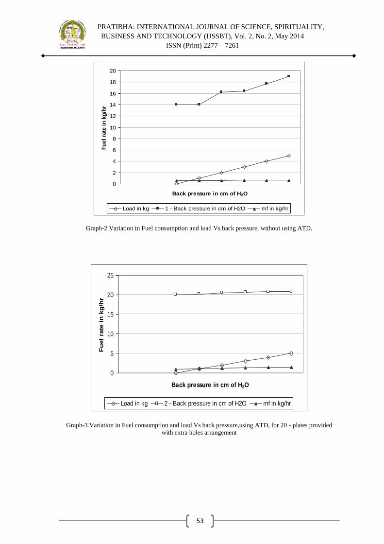
PRATIBHA: INTERNATIONAL JOURNAL OF SCIENCE, SPIRITUALITY,
BUSINESS AND TECHNOLOGY (IJSSBT), Vol. 2, No. 2, May 2014
ISSN (Print) 2277—7261
53
Graph-2 Variation in Fuel consumption and load Vs back pressure, without using ATD.
Graph-3 Variation in Fuel consumption and load Vs back pressure,using ATD, for 20 - plates provided
with extra holes arrangement
0
2
4
6
8
10
12
14
16
18
20
Back pressure in cm of H2O
Fu
el
rate
in
kg
/hr
Load in kg 1 - Back pressure in cm of H2O mf in kg/hr
0
5
10
15
20
25
Back pressure in cm of H2O
Fu
el
rate
in
kg
/hr
Load in kg 2 - Back pressure in cm of H2O mf in kg/hr

PRATIBHA: INTERNATIONAL JOURNAL OF SCIENCE, SPIRITUALITY,
BUSINESS AND TECHNOLOGY (IJSSBT), Vol. 2, No. 2, May 2014
ISSN (Print) 2277—7261
54
Graph-4 Variation in brake thermal efficiencies Vs back pressure, 1- without using ATD & 2- With ATD,
20 plates provided with extra holes arrangement at various load conditions.
Graph-5 Variation in filtration efficiencies Vs back pressure, using ATD with different no. of plate‘s
arrangement.
1 - Without using DPF.
2- using DPF, 20 plates provided
with extra holes arrangement
0
5
10
15
20
25
1 - Brake Thermal Efficiency in % 1 - Back pressure in cm of H2O
2 - Brake Thermal Efficiency in % 2 - Back pressure in cm of H2O
-20
-10
0
10
20
30
40
50
60
70
80
Back pressure in cm of H2O
Fil
tera
tio
n e
ffic
ien
cy i
n %
Back pressure in cm of H2O Filteration efficiency in %

PRATIBHA: INTERNATIONAL JOURNAL OF SCIENCE, SPIRITUALITY,
BUSINESS AND TECHNOLOGY (IJSSBT), Vol. 2, No. 2, May 2014
ISSN (Print) 2277—7261
55
Graph-6 Comparison of NOx emissions conversion efficiency at different exhaust conditions
Graph-7Comparison of HC emissions conversion efficiency at different exhaust conditions
0
5
10
15
20
NOx in %
Without DPF
With DPF (8 plates arrangement)
With DPF ( 15 plates arrangement)
With DPF ( 20 plates arrangement)
With DPF ( 20 plates with extra 5mm dia. Hole arrangement)
0
10
20
30
40
50
60
HC in %
Without DPF
With DPF (8 plates arrangement)
With DPF ( 15 plates arrangement)
With DPF ( 20 plates arrangement)
With DPF ( 20 plates with extra 5mm dia. Hole arrangement)

PRATIBHA: INTERNATIONAL JOURNAL OF SCIENCE, SPIRITUALITY,
BUSINESS AND TECHNOLOGY (IJSSBT), Vol. 2, No. 2, May 2014
ISSN (Print) 2277—7261
56
Graph-8Comparison of CO emissions conversion efficiency at different exhaust conditions
9) CONCLUSIONS
To minimize the pumping work, the
backpressure must be as low as possible for
obtaining the maximum output from the engine.
The backpressure is directly proportional to the
pressure drop across the After Treatment Device or
design of complete exhaust system components
causes the back pressure. The reported
regeneration technique infers good, quick and
economical activity. Improvement of filter and
engine exhaust flow area design is likely to make
these low cost materials practically feasible.
It is necessary not just too adequately
implement after treatment techniques in new
technology, but also the older technology engines
which are still on the road. Basic causes of
increase in backpressure & remedial actions are
suggested in this work. Regeneration phenomenon
particularly in C.I. engine after treatment devices
specifically requires attention because of
noncombustible Particulate Matter constituent‘s
accumulations.
ACKNOWLEDGEMENTS
Two authors Mr. Prashant P. Bornare and Dr. D.S.
Deshmukh are thankful to the SSBT‘s Collage of
Engineering & Technology, Bambhori Jalgaon for
providing financial assistance and research
laboratory facility for experimentation work.
REFERENCES [1] Nitin K. Labhsetwar, A. Watanabe and T. Mitsuhashi,
―Possibilities of the application of catalyst technologies for the control of particulate emission for diesel vehicles‖,
SAE Transaction 2001, paper no. 2001-28-0044.
[2] J.B. Heywood; ―Internal Combustion Engine Fundamentals‖; McGraw –Hill, ISBN 0-07-100499-8,
1988. [3] Hilbert Schenck Jr., Theories of engineering
experimentation, McGraw-hill book publishing company.
[4] D.S. Deshmukh, J.P. Modak and K.M. Nayak, "Experimental Analysis of Backpressure Phenomenon
Consideration for C.I. Engine Performance Improvement"
SAE Paper No. 2010-01-1575, International Powertrains,
Fuels & Lubricants Meeting, Rio De Janeiro, Brazil, on
dated- 5 May 2010.
[5] D.S. Deshmukh, M.S. Deshmukh and J.P. Modak, ―Experimental Investigation of Effects of Operating
Variables on a C. I. Engine Performance,‖ International
Journal of Industrial Engineering and Technology (IJIET). ISSN 0974-3146 Volume 2, Number 1 (2010), pp. 197--
206
[6] D.S. Deshmukh, M.S. Deshmukh and J.P. Modak, ―Design Considerations for Diesel Particulate Filter for
Enhancement of Engine Performance and Emission
Control" International Journal of Engineering Research and Technology. ISSN 0974-3154 Volume 3, Number 3
(2010), pp. 761--774
[7] D.S. Deshmukh, M.S. Deshmukh and J.P. Modak, "Experimental Investigation of the Effect of Backpressure
on an I.C. Engine Operating Performance" international
journal of emerging technologies and applications in engineering, technology and sciences (IJ-ETA-ETS)
(ISSN: 0974-3588 I APRIL 2010) Page no. 23-28.
[8] D.S. Deshmukh, M.S. Deshmukh and J.P. Modak, "Experimental Investigation of the Effect of Backpressure
on an I.C. Engine Operating Performance", International
Conference ICSES – 10, organized by S.E.S. College of Engineering, Navalnagar on dated 1 - 2 April - 2010.
[9] D.S. Deshmukh and P.V. Mahajan, "Formulation of
Mathematical Model for the study of effect of Backpressure on a C.I. Engine Performance", at ICSES –
10, International Conference organized by S.E.S. College
of Engineering, Navalnagar on dated 1 - 2 April - 2010. [10] M.S. Deshmukh, D.S. Deshmukh and J.P. Modak.
"Experimental Investigation of Diesel Particulate Filter
System on Single cylinder Stationary C. I. Engine‖ at ICEEE – 2009, International Conference organized by
Mulshi Institute of Technology and Research, Sambhave,
Mulshi, Pune.on dated 16- 18 February - 2009.
0
2
4
6
8
10
CO in %
Without DPF
With DPF (8 plates arrangement)
With DPF ( 15 plates arrangement)
With DPF ( 20 plates arrangement)
With DPF ( 20 plates with extra 5mm dia. Hole arrangement)

PRATIBHA: INTERNATIONAL JOURNAL OF SCIENCE, SPIRITUALITY,
BUSINESS AND TECHNOLOGY (IJSSBT), Vol. 2, No. 2, May 2014
ISSN (Print) 2277—7261
57
[11] D.S. Deshmukh, M.S. Deshmukh and J.P. Modak.
"Possible Causes And Remedies For Backpressure Rise
Problem In C. I. Engine System‖ at ICEEE – 2009, International Conference organized by Mulshi Institute of
Technology and Research, Sambhave, Mulshi, Pune.on
dated 16- 18 February - 2009. [12] D.S. Deshmukh, M.S. Deshmukh and A.A. Patil "Design
Considerations For Energy Efficient C. I. Engine Exhaust
System‖ at ICEEE – 2009, International Conference organized by Mulshi Institute of Technology and
Research, Sambhave, Mulshi, Pune.on dated 16- 18
February - 2009. [13] D.S. Deshmukh and M.S. Deshmukh, ―Effect of back
pressure on exhaust after treatment system development
for C.I. engine‖ at Team Tech – 2008, International Conference organized by I.I.Sc. Bangalore on dated- 22
Sep.2008 -24 Sep. 2008.
[14] D.S. Deshmukh and J.R. Choudhari, ―E.G.R. systems for
Diesel engines : A Critical review‖ at IME-07, National
Conference organized by department of mechanical
engineering, J.T.Mahajan College of engineering, Faizpur, from March 29 – 30, 2007.
[15] D.S. Deshmukh and M.S. Deshmukh,―Reduction of
emission using Catalytic Converter‖ National level technical Symposium held at L.I.T. Nagpur, VERVE2K3.
[16] A.A. Patil, D.S. Deshmukh, L.G. Navale and V.S. Patil, ―Experimental Investigation of a C.I. Engine Operating
Parameters for Energy Efficient Exhaust System
Development" International Journal of Innovations in Mechanical & Automobile Engineering (IJIMAE), ISSN
2249-2968 (Print), Sept.2011, Issue – I, Vol. -II, pp. 60-64
[17] Dheeraj S. Deshmukh, M.S. Deshmukh, P D. Patil and S.U. Patel, ―Development of Experimental Data Based
Model for Backpressure Generation Phenomenon on a
Stationary C.I. Engine" International Journal of Innovations in Mechanical & Automobile Engineering
(IJIMAE), ISSN 2249-2968 (Print), Nov.-.2012, Issue –
III, pp. 27-48. [18] Dheeraj S. Deshmukh, M.S. Deshmukh, P D. Patil and
S.U. Patel, ―Experimental Investigation on an Internal
Combustion Engine for Operating Performance Enhancement" International Journal of Innovations in
Mechanical & Automobile Engineering (IJIMAE), ISSN
2249-2968 (Print), Nov.-.2012, Issue – III, pp. 136-156. [19] Dheeraj S. Deshmukh, M.S. Deshmukh, and A. A. Patil,
―Investigation of Factors Affecting the After Treatment
Device Design for a Compression Ignition Engine" International Journal of Innovations in Mechanical &
Automobile Engineering (IJIMAE), ISSN 2249-2968
(Print), Nov.-.2012, Issue – III, pp. 102- 118. [20] Dr. Dheeraj S. Deshmukh, Dipak C. Talele and M.V.
Kulkarni ―Development of Mathematical Model for
Stationary Compression Ignition Engine Performance Analysis‖ in Pratibha: International Journal of Science,
Spirituality, Business and Technology (IJSSBT), ISSN
(Print) 2277-7261 and ISSN (on-line):2278-3857, Page
No. 8-17, Volume 2, No.1, November, 2013.

PRATIBHA: INTERNATIONAL JOURNAL OF SCIENCE, SPIRITUALITY,
BUSINESS AND TECHNOLOGY (IJSSBT), Vol. 2, No. 2, May 2014
ISSN (Print) 2277—7261
58
INTERLOCKING BRICK FOR SUSTANABLE HOUSING
DEVELOPMENT
R. K. Watile(1)
,S. K. Deshmukh1, H.C.Muley
1
1Department of Civil Engineering, C.O.E. &T., Akola (MS), India.444104
E-mail: [email protected]
Abstract:
The use of interlocking bricks masonry has
gained rapid popularity in many foreign
countries as an alternative to conventional
bricks for sustainable housing. It is being
always challenge for researchers to make
interlocking brick light weight, low cost and
improve the performance against aggressive
environment. An experimental effort made in
this concern. This paper gives the results of an
experimental investigation in which the
compressive strength, water absorption and
density were investigated by using varying
percentage of fly ash, stone dust, and sand with
different mix proportion. A manmade fibre,
glass fibre reinforce polymer (GFRP) utilize as
reinforcing material to produce the interlocking
blocks which gives appreciable results discuss in
detail. The experimental results compared with
that ordinary brunt clay brick and interlocking
brick found durable in aggressive environments
and have sufficient strength for their use in
sustainable building construction.
Key Words: Fly Ash, GFRP, Compressive
Strength, Water Absorption, Density
1. INTRODUCTION
A very high amount of waste is being produced all
around the world. The most common method of
managing waste is through its disposal in landfills
creating in that way huge deposits of waste. In this
situation, waste recycling is gaining increasing
importance [1]. At present in India, about 206
coals based thermal power plants are producing
about 160 million tons of fly ash every year; the
estimates prepared by Ministry of Power as well as
Planning Commissions up to the year 2031-32
indicate that generation of fly ash during the year
2031-32 would be around 900 million tons per
year [2-3]. Whereas the current annual production
of fly ash worldwide is estimated around 600
million tones [4].The Government of India took
policies initiative for utilization and disposal of fly
ash [5]. In a tropical country like India the burnt
clay brick is the most basic building material for
construction of houses. It is reported that the
requirement of bricks for construction activity
amounts to be more than 140 billion numbers
annually [6]. For fulfill such demand fly ash
interlocking brick may be one of alternative for
sustainable construction industry.
Much experimental research carried out for
producing good quality brick with reduction of
cost using industrial waste [7]. And also for
reducing price and increasing the strength many
natural and manmade reinforcing material used in
the production of bricks. There are a wide range of
natural fibres, namely sisal, bamboo, coir (coconut
fibre), jute, and many others [8]. In this research
work the manmade fibre GFRP introduce as a
reinforcing material. The effect of GFRP with
maximum percentage of fly ash in interlocking
brick is studied. This advocate the use of fly ash as
the supplementary material to soil by reducing the
consumption of soil in brick manufacturing
towards efforts of maintaining ecological balance
through sustainable development of natural
resources. The dry stacked stabilized interlocking block masonry replaces the conventional burnt clay brick and mortar construction masonry. The use of interlocking bricks masonry has gained rapid popularity in many foreign countries as an alternative to conventional bricks for sustainable housing [9].Interlocking block masonry
The dry stacked stabilized interlocking block
masonry replaces the conventional burnt clay brick
and mortar construction masonry. The use of
interlocking bricks masonry has gained rapid
popularity in many foreign countries as an
alternative to conventional bricks for sustainable
housing [9].Interlocking block masonryby
Hydraform (or by others) is one such building
system which almost full fills all such
requirements of being a sustainable masonry [10-
11].As per IS code bricks are designated based on
their average compressive strength [12-13]. Indian
masonry design standard does not deal with dry
interlocking block masonry, hence does not
prescribe the design values for this masonry like
basic compressive, tensile and shear
stressHowever the same code recognizes some
other types of masonry and recommends that a
prism test of different masonry may be done and
these values may be accepted for designing the
masonry [14]. Interlocking bricks in central India
made with locally available raw materials have the
density around 25-30 kN/m3& avg. comp. strength
is 2-4 MPa [15]. Due to this high weight & low
compressive strength it is not possible to use this
bricks in multistoried building. Density can be
reducing with increase in compressive strength

PRATIBHA: INTERNATIONAL JOURNAL OF SCIENCE, SPIRITUALITY,
BUSINESS AND TECHNOLOGY (IJSSBT), Vol. 2, No. 2, May 2014
ISSN (Print) 2277—7261
59
through experiment which may provide the best
solution for such type of bricks.
2. EXPERIMENTAL PROGRAMME
2.1 Material
For casting of interlocking bricks locally available
raw materials like fly ash, stone dust, marble slurry
and sand were used. Additional material GFRP
was used to investigate the effect on properties of
interlocking brick.
2.1.1 Cement
Ordinary Portland cement were used satisfying all
the IS requirements was used in making the bricks
[16]. The physical properties of cement listed in
Table no.1
2.1.2 Fly Ash
The fly ash (see fig 1.a) was collected in dry state
from the Paras Thermal power station and the
chemical characteristics of the fly ash are given in
Table 2.
Table 1
Material Physical
Properties
Value
Cement
Specific gravity 3.18
Specific surface 2250 cm2/gm
Soundness 1 mm
Initial setting time 35 min
Final setting time 380 min.
Compressive
Strength
(1:3 cement sand
mortar)
19.2 MPa(3
days)
28.5 MPa(7
days)
Table 2
Material Chemical
Constituents
Percentage
Fly ash
Silica ( as SiO2) 64.23 %
Alumina (as
Al2O3)
25.82 %
Iron (as Fe2O3) 4.06 %
Sodium (as Na2O) 0.40 %
Sulphur Trioxide
(as SO3)
0.27 %
Magnesium Oxide
(as MgO)
0.78 %
Loss of ignition
(as I.OI)
0.39 %
2.1.3 Fine Aggregate
Sand i.e., fine aggregate obtained locally from
nearest river passing through 4.75 IS sieve having
fineness modulus (F.M)-2.61 and confirming to
zone-III as per IS: 383-1970 [17] and its physical
properties are enlisted in Table 3.
2.1.4 Stone dust
Powder form stone dust (see fig. 1.b) available
locally used in moderate quantity for preparing the
bricks. Its fine size make possible to retain proper
shape of the bricks particularly maintaining the
edges and corners.
2.1.5 GFRP
GFRP used as reinforcing material (see fig. 1.c);
the physical properties are listed in Table 3.
Fig. No. 1.a Fly ash
1.b Stone Dust
1.C GFRP
Table 3

PRATIBHA: INTERNATIONAL JOURNAL OF SCIENCE, SPIRITUALITY,
BUSINESS AND TECHNOLOGY (IJSSBT), Vol. 2, No. 2, May 2014
ISSN (Print) 2277—7261
60
2.1.6 Water
Ordinary tap water was used for both mixing the
constituents of the bricks as well as for the curing
of bricks.
2.2 Process operation
2.2.1 Casting of interlocking bricks
For casting the Cement and other constituents were
used randomly in varying proportions of 1:10, 1:11
and 1:12. In order to establish the feasibility of
producing a binder that can impart adequate
strength, three specimen bricks were casted for
each mix proportions given in Table 4. A pan
mixer and hydraulic machine used for casting the
bricks (see fig. 2.a). Before casting the bricks,
mixer was properly cleaned. Cement and stone
dust were added in dry state, mixed thoroughly and
then clean potable water was added to get a mix of
desired workability. The mix so prepared for the
bricks was then poured in hydraulic machine and
bricks were then taken out of it and kept over level
surface under the shed for drying purpose. The
blocks have geometric size of
230mmx100mmx75mm (see.fig 2.b & c). This
machine produces solid blocks of laterite
composition mainly and stabilized with cement
material.
Fig. No.2.a Hydraulic Machine 2.b Interlocking
Brick (Ridge) 2.c Interlocking Brick (Bed)
2.2.2 Curing
The green bricks were allowed for surface dry for
one day and cured normally for 28 days by
spraying water four to five times in one day (see
fig.3.a). After gaining sufficient strength they were
submerged in water and sulphate solution at
normal room temperature of 27 + 2oC for different
ages. Sulphate solution having sulphate (SO4)
concentration equal to 10000 ppm was prepared in
laboratory by mixing 14.79 gm NaSO4 in one liter
of water.
2.2.3 Testing
The casted bricks were taken out from water one
day prior to the testing and were tested for
compressive strength after 14, 28 and 90 days and
water absorption test as per IS 1077-1957 Code.
2.2.3.1 Compressive Strength Test Procedure
Compressive strength test should be done in
compression testing machine. Blocks should be
placed between the jaws and load should be
applied gradually. Precaution should be taken such
that load should be applied to the flanged portion
of the blocks. For this cement mortar of proportion
Material Properties Value obtained
Sand
Specific
Gravity
2.48
Water
Absorption
1.05
Bulking of
Sand
26.84%
Free Moisture 1.00%
Bulk Density 1500 kg/m3
Stone dust
Specific
Gravity
2.68
Water
Absorption
0.32%
Fineness
Modulus
2.89
Silt Content 2.1%
GFRP
Nominal dia. 0.09 mm
Tensile
strength
25 N/mm
Type of wave Plane

PRATIBHA: INTERNATIONAL JOURNAL OF SCIENCE, SPIRITUALITY,
BUSINESS AND TECHNOLOGY (IJSSBT), Vol. 2, No. 2, May 2014
ISSN (Print) 2277—7261
61
1:3 are placed on top flange as well as at bed and
gradual load is applied over the complete area till
the failure occurs and not the maximum load at
failure (see fig 3.b). The load at failure shall be the
maximum load at which the specimen fails to
produces any further increase is the indicator
reading on compression testing machine (see fig
3.c).
The test report shall be given below:
Compressive strength = Maximum load at failure
Avg. area at bed face
The compressive strength of any individual block
shall not fall below the minimum average
compressive strength by more than 20% as per IS
1725-1982 [18].
Fig. No. 3.a Curing 3.b Interlocking Brick 3.c CTM Testing
2.2.3.2 Water Absorption Test
Bricks have pores in them. Due to porosity, the dry
bricks when come into contact with water absorb
water through these pores. Smaller the porosity;
lesser is the absorption. Formula to calculate water
absorbed by the bricks, using following formula:
[(w2- w1) / w1] x100
2.2.3.3 Density
230 mm
75 mm
Mortar
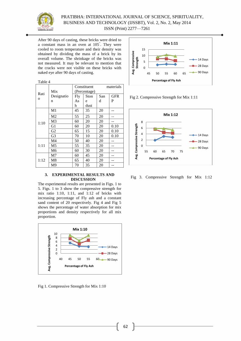
PRATIBHA: INTERNATIONAL JOURNAL OF SCIENCE, SPIRITUALITY,
BUSINESS AND TECHNOLOGY (IJSSBT), Vol. 2, No. 2, May 2014
ISSN (Print) 2277—7261
62
After 90 days of casting, these bricks were dried to
a constant mass in an oven at 105°. They were
cooled to room temperature and their density was
obtained by dividing the mass of a brick by its
overall volume. The shrinkage of the bricks was
not measured. It may be relevant to mention that
the cracks were not visible on these bricks with
naked eye after 90 days of casting.
Table 4
Rati
o
Mix
Designatio
n
Constituent materials
(Percentage)
Fly
As
h
Ston
e
dust
San
d
GFR
P
1:10
M1 45 35 20 --
M2 55 25 20 --
M3 60 20 20 --
G1 60 20 20 0.10
G2 65 15 20 0.10
G3 70 10 20 0.10
1:11
M4 50 40 20 --
M5 55 35 20 --
M6 60 30 20 --
1:12
M7 60 45 20 --
M8 65 40 20 --
M9 70 35 20 --
3. EXPERIMENTAL RESULTS AND
DISCUSSION
The experimental results are presented in Figs. 1 to
5. Figs. 1 to 3 show the compressive strength for
mix ratio 1:10, 1:11, and 1:12 of bricks with
increasing percentage of Fly ash and a constant
sand content of 20 respectively. Fig 4 and Fig 5
shows the percentage of water absorption for mix
proportions and density respectively for all mix
proportion.
Fig 1. Compressive Strength for Mix 1:10
Fig 2. Compressive Strength for Mix 1:11
Fig 3. Compressive Strength for Mix 1:12
02468
10
40 45 50 55 60
Avg
. Co
mp
ress
ive
Str
en
gth
Percentage of Fly Ash
Mix 1:10
14 Days
28 Days
90 Days
0
5
10
15
45 50 55 60 65Avg
. Co
mp
ress
ive
St
ren
gth
Percentage of Fly Ash
Mix 1:11
14 Days
28 Days
90 Days
0
2
4
6
8
55 60 65 70 75
Avg
. Co
mp
ress
ive
Str
en
gth
Percentage of Fly Ash
Mix 1:12
14 Days
28 Days
90 Days

PRATIBHA: INTERNATIONAL JOURNAL OF SCIENCE, SPIRITUALITY,
BUSINESS AND TECHNOLOGY (IJSSBT), Vol. 2, No. 2, May 2014
ISSN (Print) 2277—7261
63
Fig 4.%Water absorption of interlocking bricks
Fig 4.%Water absorption of interlocking bricks
Fig 5. Density of interlocking brick
Fig 6. Compressive Strength for Mix 1:10 GFRP
Fig 7. % Water absorption of Mix 1:10 GFRP
Fig 8. Density of Mix 1:10 GFRP
Figs. 1, 2 shows that the compressive strength of
interlocking brick initially increases with the
increase in fly ash content but fig.3 after attaining
a maximum value it start decreasing with the
further addition of fly ash. Fig 4 shows the water
absorption of interlocking bricks. It is observed
that in general, the water absorption of bricks
increases with the increase in fly ash content
replacing stone dust. On comparing interlocking
bricks with ordinary burnt clay bricks it is
observed that water absorption of interlocking
bricks in the present investigation was obtained in
between 6.42 to 12.4 percent whereas the water
absorption of ordinary bricks shall not be more
than 20 percent by weight. Density of interlocking
bricks is shown in Fig. 5. It is observed that the
water absorption and density are closely related to
each other. The density of interlocking bricks was
found to be 7.5 to 25 percent higher than that of
the ordinary burnt clay bricks.
GFRP a reinforcing material plays vital role with
increase in percentage of fly ash. Its influence
make increase in compressive strength, lesser
water absorption and density reduce up to 20
0
2
4
6
8
10
12
14
40 45 50 55 60 65 70 75
% W
ate
r A
bso
rpti
on
% Fly Ash
Mix 1:10
Mix 1:11
Mix 1:12
21.5
22
22.5
23
23.5
24
24.5
25
25.5
40 45 50 55 60 65 70 75
De
nsi
ty k
N p
er
Cu
b.M
.
% Fly Ash
Mix 1:10
Mix 1:11
Mix 1:12
0
5
10
15
60 65 70
Avg
. Co
mp
ress
ive
Str
en
gth
N/m
m2
Mix 1:10 GFRP
14 Days
28 Days
90 Days
Percentage of Fly ash
8
9
10
11
60 65 70% W
ate
r A
bso
rpti
on
Mix 1:10 GFRP
Water Absorption %
Fly ash Percentage
20
20.5
21
21.5
60 65 70
De
nsi
tykN
/Cu
.M.
Mix 1:10 GFRP
Density kN/Cu.…
Fly ash Percentage

PRATIBHA: INTERNATIONAL JOURNAL OF SCIENCE, SPIRITUALITY,
BUSINESS AND TECHNOLOGY (IJSSBT), Vol. 2, No. 2, May 2014
ISSN (Print) 2277—7261
64
percent comparing with initial density of
interlocking brick.
CONCLUSIONS
Based on the experimental investigation reported
in this paper, following conclusions are drawn:
1. Strength of interlocking bricks with
increasing fly ash increases with the age.
2. All mix proportions gives satisfactory
higher values of compressive strength.
3. At some without GFRP mix ratio 1:11 gives
the higher compressive strength greater than
10 N/mm2.
4. Interlocking bricks with economically
available fly ash in large proportion have
sufficient strength for their use in low cost
housing, non-load bearing construction and
in regions where good quality burnt clay
bricks are not available.
5. Water absorption of interlocking bricks
without GFRP is found to be in the range of
6.42 to 12.4 percent, whereas the water
absorption for ordinary burnt clay bricks
should not be more than 20 percent. The
water absorption of interlocking bricks
increases with the increased fly ash content.
6. The density of interlocking bricks was
found to be 7.5 to 25 percent higher than
that of the ordinary burnt clay bricks.
7. Interlocking brick with reinforcing agent
GFRP increases the compressive strength at
maximum utilization of fly ash with the age.
8. The water absorption and density increase
with increase in fly ash in GFRP
interlocking brick.
9. As density concern the difference between
ordinary clay brick and interlocking brick
should be minimize with reinforcing agent.
Interlocking bricks require no skilled labour and
can be moulded in any shape and size depending
on the requirements. These bricks have better
tolerances and no efflorescence as compared to
conventional bricks. A number of other benefits
also be ascribed for the prospect of interlocking
bricks which includes no consumption of mortars,
better efficiency in laying and low cost of
finishing. It is further needed to develop the
awareness among users, professionals and
financial supporters for using these waste materials
for solving the housing problems in addition to
balance economy and achieve energy conservation.
For reducing the density of bricks more
experimentation requires with different wasted
material with natural reinforcing fibre for
considering economy and use for multistoried
building.
REFERENCES
[1] Correia S L, Souza F L, Dienstmann G, Segadaes A M, ―
Assessment of the recycling potential of fresh concrete waste using a factorial design of experiments‖, Waste
Manage 2009; 29:2886-91. [2] Jain A K, ―Fly Ash Utilization in Indian Cement Industry:
Current Status and Future Prospects‖, Indian Concrete
Institute, an Electronic Bulletin, Vol. 2, Issue 2, Feb.2011. [3] R and D Proposals, Department of Science and
Technology, Ministry of Science & Technology,
Government of India, December, 2012. [4] Uygunog˘lu T , Topcu I B, Gencel O, Brostow W, ―The
effect of fly ash content and types of aggregates on the
properties of pre-fabricated concrete interlocking blocks (PCIBs)‖, Construction and Building Materials 30 (2012)
180-187.
[5] Dhadse S, Kumari P, Bhagia L J, ―Fly Ash
Characterization, Utilization and Government Initiatives
in India- A Review‖, Journal of Scientific and Industrial
Research, Vol. 67, January 2008, 11-18. [6] Model Project Report,Punjab State Council for Science
and Technology, June 2010.
[7] Kadir A, Mohajerani A, ―Brick: An Excellent Building Material for Recycling Wastes- A Review‖, International
Conference on Environmental Management and
Engineering (EME 2011), July2011, Canada. [8] Ali M, Gultom R J, Chouw N, ―Capacity of Innovative
Interlocking Blocks under Monotonic Loading‖,
Construction and Building Materials 37 (2012) 812-821. [9] Kintingu S H, ―Design Of Interlocking Bricks for
Enhanced Wall Construction Flexibility, Alignment
Accuracy And Load Bearing‖, Ph.D. Thesis, The University of Warwick, School of Engineering, May
2009.
[10] Bansal D, ―Interlocking Dry Stacked Masonry‖, 8th International Masonry Conference 2010 in Dresden.
[11] Adedeji Y M D and Fa G, ―Sustainable Housing
Provision: Preference for the Use of Interlocking Masonry in Housing Delivery in Nigeria‖, Journal of
Environmental Research and Management Vol. 3(1). pp.
009-016, January, 2012. [12] BIS, Common Burnt Clay Building Bricks-
Specification:Fifth Revision IS 1077:1992.
[13] BIS, Burnt Clay Fly Ash Building Bricks Specification, I.S. Code 13757:1993.
[14] BIS, Code of Practice for Structural Use of Unreinforced
Masonry, Third Revision IS 1905:1987. [15] Watile R K, Deshmukh S K, Gawatre D W, ―Performance
of Fly-Ash Interlocking Brick‖, International Journal for
Civil Engineering and Technology,Volume 4, Issue 6, November – December (2013), 82-88.
[16] BIS, Specification for 53 Grade Ordinary Portland cement
IS: 12269 -1987. [17] BIS, Specification For Coarse And Fine Aggregates From
Natural Sources For Concrete:Second Revision IS:
383:1970. [18] BIS, Specification For Soil Based Blocks Used In General
Construction: Fifth Revision IS 1725-1982.

PRATIBHA: INTERNATIONAL JOURNAL OF SCIENCE, SPIRITUALITY,
BUSINESS AND TECHNOLOGY (IJSSBT), Vol. 2, No. 2, May 2014
ISSN (Print) 2277—7261
65
INTEGRATED RELIABILITY EVALUATION OF
DISTRIBUTED POWER SYSTEM
Apeksha Narendra Rajput1, Bharti Drivedi
2, Anurag Tripathi
3
1Research Scholar, Indraprastha Engineering College
Electrical Engg.Deptt.Ghaziabad, (U.P), India, 2Professor, Electrical Engg. Department,
Institute Of Engineering and Technology, Luck now (Uttar Pradesh), India 3Associate Professor, Electrical Engg. Department,
Institute Of Engineering and Technology, Luck now (Uttar Pradesh), India [email protected] [email protected]
Abstract—This various distribution system
designs, including Distributed Energy
Resources (DER), affect distribution reliability
indices, System Average Interruption Duration
Index (SAIDI) and System Average
Interruption Frequency Index (SAIFI)
Furthermore, This presents an example for
optimization of distribution maintenance
scheduling of a recloser. It applies a risk
reduction technique associated with
maintenance of the equipment.Given a large
and complex plant to operate, a real-time
understanding of the networks and their
situational reliability is important to
operational decision support.
IndexTerms—reliability, distribution system,
equipment, power quality, active power, reactive
power.
1. INTRODUCTION
Reliability of a power system is generally
designated as a measure of the ability of the system
to provide customers with adequate supply. It is
one of the primary performance criteria of power
systems. Major outages can have a significant
economic impact on utility providers as well as the
end users who lose electric service. The power
system has been significantly affected by a wide
range of outage events caused by incorrect
planning, operational error, equipment failures,
environmental conditions, adverse weather effects,
and load conditions. Large-scale blackouts
emphasize the importance of reliability issues.
The reliability evaluation of transmission or
composite systems analyzes the system failure
events and estimates the chances of loss of load at
major load points . The reliability of distribution
systems is based on individual customer service
interruptions. Since the reliability studies described
in this dissertation are customer service oriented,
one of the analysis zones of the study includes the
whole distribution system with extension to the
sub-transmission lines and substations.
For some of the networks analyzed here, the
dominant causes of customer power interruptions
are problems in secondary networks and faults in
sub-transmission systems. Therefore, just
considering the distribution system itself is not
enough to accurately estimate customer outages.
2. CHALLENGES IN SYSTEM MODELING
AND RELIABILITY ANALYSIS
The modeling and analysis studies associated with
reliability evaluation are challenging, not only
because of some of the system characteristics of
the above proposed analysis zones, but also for
persistent problems that have lingered in the
energy industry for decades.
(i) Size. The reliability evaluation of large utility
systems can be daunting due to the sheer size of
the model. Modeling the underlying distribution
system, including each customer‘s service point,
can result in a model containing millions of
objects. Relatively scant attention has been given
to distribution systems as compared to generation
and transmission systems. However, as the
distribution system could be 80% larger than the
transmission system, and occupies as much as 40%
of the overall capital outlay of the total grid , it
should receive adequate attention.
(ii) Data. The modeling and reliability analysis of
distribution and/or transmission systems involves a
large volume of various types of data and multiple
system analysis algorithms. Examples of data

PRATIBHA: INTERNATIONAL JOURNAL OF SCIENCE, SPIRITUALITY,
BUSINESS AND TECHNOLOGY (IJSSBT), Vol. 2, No. 2, May 2014
ISSN (Print) 2277—7261
66
include load, operation, planning, system design,
system description, and reliability data. Examples
of computer program algorithms include load flow,
load forecast, network topology tracking and
updating, and reliability analysis. Integrating the
data into knowledge that is efficiently used by
algorithms, and ensuring cooperation among
algorithms are challenging tasks .
(iii) Load. The electrical load varies from hour to
hour, day to day, and season to season. Each type
of customer usually has different usage patterns.
Residential, commercial, and industrial customers
have different power demands and different peak
demand times. This non-linear, time-varying
characteristic has to be considered in order to
obtain sound system evaluation results.
(iv) Uncertainty. The power system is vulnerable
to many stochastic events. Random failures of
control and protection devices, environmental
disturbances such as high speed wind, lightning
and severe storms, irregular load surges due to
interruptions, and human errors all have impacts
on customer outages.
3. INTEGRATED RELIABILITY EVALUATION OF
POWER SYSTEMS
The reliability evaluation of hierarchical level I
includes the generation system only. The
generating capacity needs to be determined in
order to satisfy the expected demand. The
reliability evaluation of hierarchical level II
includes generation and transmission systems,
which is often referred to as the composite system
or bulk power system. The transmission system
has to be designed to ensure satisfactory energy
transfer from generation plants to bulk load points.
The reliability evaluation of hierarchical level III
includes all the three systems, and is rarely done
due to the enormity of the problem.
Figure1 Hierarchical levels of Power System for
Reliability Analysis
During integrated system modeling, if
transmission/sub-transmission systems are
included, the boundaries of transmission systems
are treated such that the generation capacity is not
constrained. The reliability studies are then used to
examine the energy delivery capability to bulk load
points for a transmission system only study or, to
end-customers if the study zones include
distribution systems.
4. RELIABILITY ASSESSMENT METHODS
OF POWER SYSTEMS
The methods used in reliability assessments of
power systems determine the accuracy of the
results. Analytical and simulation approaches are
the two types of techniques used in power system
reliability analysis. Each approach has its merits
and limitations. In this section, the concepts,
assumptions, and typical applications of the
commonly used methods in both techniques are
reviewed. The limitations of analytical approaches
are summarized as the reason to select the Monte
Carlo simulation to perform the reliability analysis
in this study.
1. Analytical Approach
The analytical analysis methods use mathematical
models to provide solutions to a reliability
problem. Specific calculation results are obtained
for a given set of system topology and input
values. Some widely used methods are block
diagram, event tree, cut sets, fault tree, state
enumeration, and Markov modeling. Using
reliability sets in calculation is also proposed in
recent years. Their common problem is the
frequent need to make simplifying assumptions
and approximations.
2. Simulation Approaches
Compared with analytical approaches, the
simulation or Monte Carlo approach is more
universal. It provides a solution for complex
problems that is not feasible for analytical
methods. The Monte Carlo method is widely used
to simulate the stochastic behavior of systems and
actual processes. The random number generator of
the Monte Carlo simulation creates random
variants that follow the distribution functions, even
non constant hazard rates. The simulation
convergence is a fluctuating process, with the
estimated outcome closer to the true value as
sample size increases. The convergence criterion
usually uses the coefficient of variation of the
output.
3. Performance indices

PRATIBHA: INTERNATIONAL JOURNAL OF SCIENCE, SPIRITUALITY,
BUSINESS AND TECHNOLOGY (IJSSBT), Vol. 2, No. 2, May 2014
ISSN (Print) 2277—7261
67
The study zones of this study include detailed
modeling of end-customer information, and the
system evaluation goal is also customer service
oriented. SAIFI and SAIDI are the two most
popular system level reliability indices used for
customer service oriented studies [36]. SAIDI is an
abbreviation of System Average Interruption
Duration Index. It represents the average
interruption duration per customer served per year.
SAIFI denotes the System Average Interruption
Frequency Index. It is the expected number of
interruptions per customer per year. The
calculation of SAIDI and SAIFI are shown in (1.1)
and (1.2) respectively.
SAIDISYS = Sum of customer interruption durations
Total numbers of customers
(1.1)
SAIFISYS = Total number of customer interruptions
Total numbers of customers
(1.2)
The subscript sys in the above equations denotes
that individual reliability indices can be calculated
for each aggregated network, and only considers
the customers served by the network. There are a
total of 18 aggregate networks defined in the
secondary distribution system containers. The
whole secondary distribution system can be
viewed as the largest aggregate network, with the
120V and 480V networks as individual aggregated
networks.
Instead of selecting SAIFI and SAIDI, CAIDI and
CAIFI are chosen as the reliability indicators for
this study, because they give details of the
interruption statistics of each customer. CAIDI is
abbreviation of Customer Average Interruption
Duration Index. It represents the average
interruption duration for those customers served by
the same load bus per year. CAIFI denotes for
Customer Average Interruption Frequency Index.
It is the expected number of interruptions of
customers served by a load bus per year.
The calculation of CAIDI and CAIFI is shown in
(1.3) and (1.4) respectively.
CAIDI =Sum of Customer Interruption Durations
Total Numbers of Customers Interruptions
(1.3)
SAIDI = Total number of customer interruption
Total numbers of customers Affected
(1.4)
5. CALCULATION AND RESULTS
5.1 Calculation of Reliability Indexes
SUB A
OH1
NO.OF CUSTOMER=1500
Figure 2 Distribution model
The procedure and calculations to find SAIFI for a
distributed model, as shown in Figure 2 , are
provided in detail below. All required data to
calculate SAIFI are given in Table 1.
In this example, it is assumed that the coordination
failure rate of all over current devices (fuses and
over current relays or OCRs) is 0.0. That is, in all
fault situations, each fuse or OCR operates as
required to clear the fault for all systems up line
from the fuse or OCR.
TABLE 1 RELIABILITY DATA TABLE
In this example, 1500 consumers are
connected to a Substation (SUB A) through an
overhead line (OH 1). In the Figure 2, there are no
switches or over current devices (fuses and OCRs)
in this circuit. Any fault at SUB A or OH 1 will
interrupt all 50 customers. Since only elements
with non-zero customers contribute to the total
customer interruptions, the mean failure rate can
be calculated for line element only
Calculation of System Average Interruption
Frequency Index (SAIFI):
MFR for OH 1 =FR of SUBA+FR of OH 1
= 0.1 + 0.2
= 0.3
Substation Data Overhead Line
Data Other
Failure Rate
(PR) = 0.1
Failure Rate (PR)
= 0.2
Open Time =
0
Repair time
(RT) = 5.0 hrs
Repair Time (RT)
= 2 hrs
Time to Find
Problem = 0
Close time (CT)
= 0.5 hrs
Travel time
= 0

PRATIBHA: INTERNATIONAL JOURNAL OF SCIENCE, SPIRITUALITY,
BUSINESS AND TECHNOLOGY (IJSSBT), Vol. 2, No. 2, May 2014
ISSN (Print) 2277—7261
68
TABLE 2 SAIFI CALCULATION TABLE
Total Customer Interruptions = 1440
Total Number of Customer served = 1500
Therefore
SAIFI = TotalCustomerInterruption
Total no. of Customers Served
= 1440/1500
= 0.90
Calculation of System Average Interruption
Duration Index (SAIDI):
TABLE 3 SAIDI CALCULATION TABLE
ID (SUBA) =5+0.5
Therefore
SAIDI = Customer Hour/Year
Total Customer Served
= 3150/1500
=2.107
Verification of SAIDI, and SAIFI Using
Reliability Evaluation Software
This section presents verification of the calculation
of SAIDI and SAIFI for using commercial
reliability evaluation software.
1. Select the Reliability Analysismodule from
the Analysis Modes option.
2. Select the required equipment from the tool
bar, and draw the distribution model.
3. Click the Graphical Analysis tool bar button
or select Analysis/Graphical Analysis from the
menu bar, which shows the following options.
Reliability Analysis, b. Travel Time
Calculation, c. Element Reliability Data
4. Use the Reliability Analysis tab for the
Reliability analysis settings.
5. Use the Travel Time Calculation tab for the
time setting,
6. Element Reliability Data tab provides a
Reliability Data Quick Editor option, which
allows setting reliability element data by
element category.
7. After completing the model, click the
Recalculate Analysis tab to run the reliability
analysis.
8. After running the Reliability Analysis, click
the DisplayCurrent Report tab for a summar
report.
Figure 3 Result of analysis of SAIFI and SAIDI
From the above report, we can see that SAIFI is
0.957 and SAIDI is 2.01, which verifies that the
prediction of SAIDI and SAIFI for is done
properly.
Elemen
t
F
R MFR
No. of
customer
Customer
Customer
interruption
Interruptions
SUB A 0.
1 - 0 0
OH 1 0.
2 0.3 1500 720
Total 1550 720
Outage
on
Device
Number of
Customers
Customer
Interruptio
n
Interrupti
on
Duration
(hour)
Failure
Rate
(per
year)
Custom
er
Hours
Per
Year
SUB A
7
5
0
5
.
5
0
.
1
1550
OH 1 7
5
0
2
.
5
0
.
2
1600
Total 3150
Total Customer Served: 1500

PRATIBHA: INTERNATIONAL JOURNAL OF SCIENCE, SPIRITUALITY,
BUSINESS AND TECHNOLOGY (IJSSBT), Vol. 2, No. 2, May 2014
ISSN (Print) 2277—7261
69
VARIOUS DISTRIBUTION MODELS USED
IN ANALYSIS
SUB A OH1 DER
DER
NO OF CUSTOMER= 20
Model (a)
SUB A OH1
NO OF CUSTOMER= 20 NO OF
CUSTOMER= 50
Model (b)
SUB A
OH1 OH2
NO OF CUSTOMER= 50
Model (c)
SUB A
OH 1
NO OF CUSTOMER= 20
Model (d)
SUB A OH1 OH2
NO OF CUSTOMER= 20 NO OF
CUSTOMER= 50
Model (e)
SUB A FUSE OH 1
NO OF CUSTOMER=
50
Model (f)
SUB A
OH 1
NO OF CUSTOMER= 20 NO OF
CUSTOMER= 50
Model (g)
SUB A
OH 1 OH 2
NO OF CUSTOMER= 50
Model (h)

PRATIBHA: INTERNATIONAL JOURNAL OF SCIENCE, SPIRITUALITY,
BUSINESS AND TECHNOLOGY (IJSSBT), Vol. 2, No. 2, May 2014
ISSN (Print) 2277—7261
70
TABLE 4 SUMMARIES OF DISTRIBUTION
MODELS USED IN
ANALYSIS
CONCLUSION
Although much research has been performed on
the reliability evaluation of power systems, how
large-scale realistic systems should be analyzed is
still under investigation. Various values of
reliability models and analysis are described in
Table 4.
This research makes efforts to move forward the
past works towards the direction of addressing
reliability needs directly from the consumer point
of view. Previously, electric utilities use
contingency and margin criteria for indirect
reliability measures during planning and design.
Generally, consumer oriented reliability evaluation
indices such as SAIDI and SAIFI are not directly
used in the design stage. However, given the
complexity of the realistic system with constant
facility additions and operating changes, directly
use reliability values as numeric criterion on
selecting a solution among potential alternative
designs is expected to be a trend. In this research,
the expected reliability behaviors of realistic
systems are computed by utilizing detailed analysis
of their configurations and equipment information.
REFERENCES [1] "WEST SYSTEMS COORDINATING COUNCIL
FINALREPORT,AUGUST10TH 1996 EVENT," OCTOBER 1996.
[2] WSCC, "Western Systems Coordinating Council
(WSCC)Disturbance Report for the Power System Outage that Occurred on the Western
Interconnection,August 10, 1996," approved by the
WSCC Operation Committe on October 18, 1996. [3] U.S.-Canada Power System Outage Task Force,
"FinalReport on the August 14th Blackout in the United
States and Canada," Department of Energy anNational Resources Canada2004.
[4] L. L. Grigsby, Electric Power Generation,
transmission,and distribution, 2nd ed., 2007. [5] R. N. Allan and R. Billinton, "Power system
reliabilityandits assessment. Part 2. Composite generation
and transmission systems," Power Engineering
Journal[see also Power Engineer], vol. 6, pp. 291-297,
1992.
[6] J. Endrenyi, M. P. Bhavaraju, K. A. Clements, K. J. Dhir, M. F. McCoy, K. Medicherla, N. D. Reppen, L. A.
Saluaderi, S. M. Shahidehpour, C. Singh, and J. A.
Stratton, "Bulk power system reliability concepts and applications," PowerSystems, IEEE Transactions on, vol.
3, pp. 109-117, 1988.
[7] J. Endrenyi, P. F. Albrecht, R. Billinton, G. E. Marks, N. D. Reppen, and L. Salvaderi, "Bulk Power System
Reliability Assessment-Why And How? Part I: Why?,"
IEEE Transactions on Pow Apparatus and Systems, vol. PAS-101, pp. 3439-3445, 1982.
[8] J. Endrenyi, P. F. Albrecht, R. Billinton, G. E. Marks, N.
D. Reppen, and L. Salvaderi, "Bulk Power System Reliability Assessment-Why and How? Part II: How?,"
Mod
el
No.
System
Description SAI
FI
SA
IDI Result Reason
(a) Customers
supplied
with a
source
SUB A.
Has a DER
as a backup
or
alternative
source.
Model in
Figure 5.1
has no
DER.
0.3 1.0
5
Same
value
indices
as in
Figure
1
No protecting
device between
SUB A and OH
1. DER cannot
connect if line is
still connected to
failed substation.
(b) S i m i l
i a r to
model in
Model 5.1
but with 20
additional
customers.
0.3 1.05 Same
value of
indices
as in
Model
(a)
Customers of
SUB A added to
OH 1 since no
protection device
to separate SUB
A and OH 1. 11
OH1 fails, the
substation must
be disconnected
from the entire
system.
(c) No
DER
.
Cust
omer
supplied
through
two radial
overhead
lines by a
substation.
0.5 1.55 Poorer
reliabilit
y indices
than in
Model
(b)
Addition of OH
2 adds another
component that
can fail.
(d) Same as
previous
model with
DER.
0.5 1.55 Same
value of
indices
as in
Model
(c)
No protecting
devices between
SUB A and DER
to OH 1 and OH
2.
(e) No DER.
Customers
are in each
OH line of
a radial
system.
0.5 1.55 Same
value of
indices
as in
Model
(c)
Acts like 70
customers at OH
2 since no
protective
devices between
OH 1 and OH 2.
(f) Customers
supplied
through an
OH line
that has an
over current
protecting
device.
0.3 0.95 Improve
- ment
in both
reliabilit
y indices
Protecting device
fuse used
between SUB A
and OH 1. Now,
OH 1 can be
connected to
DER.
(g) s i m i l
a r to
previous
model (f)
but 20 more
customer
added d a
the source.
0.242
8571
0.83
571
43
More
improve
d
Reliabilit
y over
Model
(f)
Better reliability.
In Model (0,
50/50 customers
are
interrup
ted but in
model
(g),50/7
0 customer are
interrupted.

PRATIBHA: INTERNATIONAL JOURNAL OF SCIENCE, SPIRITUALITY,
BUSINESS AND TECHNOLOGY (IJSSBT), Vol. 2, No. 2, May 2014
ISSN (Print) 2277—7261
71
IEEE Transactions on Power Apparatus and Systems, vol.
PAS-101, pp. 3446-3456, 1982.
[9] R. E. Brown, Electric Power Distribution Reliability: CRC, 2002.
[10] R. E. Brown, S. Gupta, R. D. Christie, S. S. Venkata, and
R. Fletcher, "Distribution system reliability assessment:
momentary interruptions and storms," Power Delivery, IEEE Transactions on, vol. 12, pp. 1569-1575, 1997.

PRATIBHA: INTERNATIONAL JOURNAL OF SCIENCE, SPIRITUALITY,
BUSINESS AND TECHNOLOGY (IJSSBT), Vol. 2, No. 2, May 2014
ISSN (Print) 2277—7261
72
REDUCED DIFFERNTIAL TRANSFORM METHOD FOR
GAS DYNAMICS EQUATION
Narhari Patil1and Avinash Khambayat
2
1Professor & Head
Department of Mathematics
Shri Sant Gajanan Maharaj College of Engineering,
Shegaon, Maharashtra, INDIA. 2 Department of Mathematics
Shram Sadhana Bombay Trusts College of Engineering &Technology,
Bambhori-Jalgaon, Maharashtra, INDIA
Abstract: The purpose of this paper is to
study the use of Reduced Differential
Transform Method (RDTM) for gas
dynamics equation and to obtain the series
solution which is more appropriate. Here we
have taken non linear gas dynamics equation
to analyze and to illustrate the effectiveness of
RDTM.
Keywords: - Reduced Differential Transform
Method, gas dynamics equation, and variational
iteration method.
1. Introduction
Reduced Differential Transform
Method [3, 5, 6, 7] belongs to basic of
Mathematical analysis. Theory of differential
equations, approximation theory, integral
transform theory, and many other area of pure
and applied mathematics. Differential Transform
Method theory is applicable to obtain solutions
of problems in partial differential equations and
ordinary differential equations, in
multidimensional, with the concept of linear and
non linear equations [10].
Many physical problems can be
described by mathematical models that involve
partial differential equations. The investigative
of the exact or approximation solution helps us
to understand the means of this mathematical
models.Sevral numerical method [1],[2],[8],[9]
were developed for solving partial differential
equations with variable coefficient such as
Homotopy perturbation method[4]. He‘s
polynomials, modified variational iteration
method.
The main goal of this paper is to apply
the reduced differential transform method to
obtain the exact solution. In many cases an
analytical approximation, in rapidly convergent
sequence for the Klein-Gordon equations. In
One dimension, the in vicid equation of gas
dynamics can be written as,
)2...()()0,(
)1...(),(),(),(2
1),(),( 22
xfxu
txgtxutxutxutxu xt
2. Reduced Differential Transform Method:
The basic definitions of RDTM are given below-
If the function u(x, t) is analytic and differential
continuously with respect to time t and space x
in the domain of interest, then let,
0
),(!
1)(
t
k
k
k txutk
xU … (3)
Where the t – dimensional spectrum function
)(xU k is the transformed function. u(x, t)
represent transformed function. The differential
inverse transform of )(xU k is defined as
follows
k
k
k txUtxu )(),(0
… (4)
Then combining equations (3) and (4) we write
0 0
),(!
1),(
k
k
t
k
k
ttxutk
txu …(5)
From the above definition, it can be found that
the concept of RDTM is derived from the power

PRATIBHA: INTERNATIONAL JOURNAL OF SCIENCE, SPIRITUALITY,
BUSINESS AND TECHNOLOGY (IJSSBT), Vol. 2, No. 2, May 2014
ISSN (Print) 2277—7261
73
series expansion. The fundamental operation
performed by RDTM can be readily obtained
and are listed in table1
Functional form Transformed form
),( txu
0
),(!
1)(
t
k
k
k txutk
xU
),(
),(),(
txv
txutxw
)()()( xVxUxW kkk
),(),( txutxw
tconsis
xUxW kk
tan
),()(
,
mmtxtxw ),(
0,0
0,1)(),()(
k
kknkxxW m
k
),().,(),( txvtxutxw )()(
0
xVUxW rkr
k
r
k
),(),( txut
txwr
r
)(.
))......(1()(
xU
rkkxW
rk
k
),(),( txux
txw
)()( xU
xxW kk
),(),(2
2
txux
txw
)()(
2
2
xUx
xW kk
We write gas dynamic equation in the standard operator form
),()),(()),(()),(( txgtxuNtxuRtxuL … (6)
With initial condition )()0,( xfxu ... (7)
Where ),()),(( txutxuL t is a linear operator which has partial derivatives.
),(),(2
1)),((
),,()),((
22txutxutxuN
txutxuR
x
and g(x, t) is in homogenous term .Using RDTM table, we construct the following iteration formula
))(())(()()()1( 1 xURxUNxGxUk kkkk … (8)
Where )()),(()),(( xGxUNxUR kkk are transformations of the functions
),()),(()),,(( txgandtxuNtxuR respectively.

PRATIBHA: INTERNATIONAL JOURNAL OF SCIENCE, SPIRITUALITY,
BUSINESS AND TECHNOLOGY (IJSSBT), Vol. 2, No. 2, May 2014
ISSN (Print) 2277—7261
74
)()().(22
)()(2
)().(22
)()(2
)(2
)(
2
120
2
120
2
10
10
1
2
0
2
0
0
xUxUxUUxUxU
xN
xUxUxUxU
xN
xUxU
xN
From initial condition (2), we write )()(0 xfxU … (9)
Substituting (9) in to (8) we get, following )(xU k values. The inverse transformation of the set of values
n
kk xU0
)(
gives approximation solution as,
n
k
k
kn txUtxu0
)(),( … (10)
Where n is order of approximation solution. Therefore the exact solution of problem is given by
),(),( lim txutxu nn
… (11)
3. Applications:-
In this section, we use RDTM for solving gas dynamic equations.
Example 1
We consider the inhomogeneous non linear gas dynamic equations.
2222 ),()1(),(2
1),( xtxuttxutxu xt … (12)
With the initial condition u(x, 0) = x …(13)
By applying differential transform (12) and the initial condition (13) respectively, we get,
)()()()1( 1 xNxFxUk kkk …(14 )
Where )(),( xNxF kk are transformed form of 2222 ),()1(),(
2
1xandtxuttxux
The transformed initial condition xxU )(0 , the equation ( 14) can be written as
)()(1
1)(1 xNxF
kxU kkk
Put k = 0, )()(10
1)( 001 xNxFxU
=
)(
2
)( 2
0
2
02 xUxU
xx
=
2
22
2x
x
xx
= x
xxU )(1

PRATIBHA: INTERNATIONAL JOURNAL OF SCIENCE, SPIRITUALITY,
BUSINESS AND TECHNOLOGY (IJSSBT), Vol. 2, No. 2, May 2014
ISSN (Print) 2277—7261
75
1=kPut , )()(11
1)( 112 xNxFxU
=2
1
)()(2
2
)(22 10
102 xUxUxUU
xx
=2
1
)(2
2
)(22 2 xx
xx
xx
= x
xxU )(2
2=kPut , )()(12
1)( 223 xNxFxU
=3
1
)(
)()(22
)()()(23
2
1
20
2
1202
xU
xUxUxUxUxU
xx
x
xxU )(3
Similarly we can obtain xxU )(4 , xxU )(5 , xxU )(6 , . . .
Then the inverse transformation of the set values n
kk xU0
)(
gives n terms approximation solution as,
n
k
k
kn txUtxu0
)(),(
nn xtxtxtxt )1(........1 32
t
x
1
which is exact solution.
Example 2:- Consider non linear homogeneous gas dynamic equation,
0),(),(2
1),(),( 22 txutxutxutxu xt
With initial condition xexu )0,( where ),( txUu is a function of the variable x and t.
The exact solution isxtetxu ),( , using the basic properties of RDTM we get transformed form of the
equation (14) as,
0)()()()1( 1 xNxUxUk kkk
)()(1
1)(1 xNxU
kxU kkk
... (15)
Where )(xNk is the transformed form of ),(),(2
1 22 txutxux
Then the transformed initial condition isxexU )(0 , … (16 )
Put k=0,
)()(10
1)( 001 xNxUxU

PRATIBHA: INTERNATIONAL JOURNAL OF SCIENCE, SPIRITUALITY,
BUSINESS AND TECHNOLOGY (IJSSBT), Vol. 2, No. 2, May 2014
ISSN (Print) 2277—7261
76
=
)(
2
)( 2
0
2
0 xUxU
xe x
= xe
!1)(1
xx e
exU
1=kPut ,
)()(11
1)( 112 xNxUxU
=2
1
)()(2
2
)()(210
10 xUxUxUxU
xe x
= 2
xe
!2)(2
xexU
2=kPut ,
)()(12
1)( 223 xNxUxU
=3
1
)()()(22
)()()(2
2
2
120
2
120 xUxUxUxUxUxU
x
e x
= 6
xe
!3)(3
xexU
Similarly we can obtain!4
)(4
xexU
, !5
)(5
xexU
, !6
)(6
xexU
, . . .
Then the inverse transformation of the set values n
kk xU0
)(
gives n terms approximation solution as,
n
k
k
kn txUtxu0
)(),(
n
n txU
txUtxUtxUtxUtxU
)(.....
....)()()()()( 4
4
3
3
2
21
0
0
=
0 !k
kx
k
te
Therefore we obtain, xtetxu ),( , Which is exact solution.
Conclusions
In this research, reduced differential transform
method has been applied for solving the gas
dynamics equation. The method is applied in a
directly without using linearization,
transformation or restrictive assumptions. The
result shows RDTM needs small size of
computation divergent to other numerical
methods. Finally it is found that RDTM is
powerful and efficient technique for finding the
exact solution.
References
[1] D.J.Evans, HBulut,Anew approach the gas dynamics
equation an application to decomposition international
Journal of Computer mathematics , 79(7)2002,817-822
[2] H.Jafri,M.Zabini,MSaidy, Application of homotopy- Perturbation method for solving gas dynamic equation,

PRATIBHA: INTERNATIONAL JOURNAL OF SCIENCE, SPIRITUALITY,
BUSINESS AND TECHNOLOGY (IJSSBT), Vol. 2, No. 2, May 2014
ISSN (Print) 2277—7261
77
applied mathematical science,2(45-48)2008,2393-
2396.
[3] Bushra A.Taha, the Use of Reduced Differential Transform Method for Solving Partial Differential
Equations with Variable Coefficients, Journal of
Basrah Researches (Sciences)) Volume 37. Number 4. C ((2011))
[4] Ylar .Keskin,Ibrahim Cagand , Ayse Betul Koc,
Numerical Solutions of sine Gorden equation equation by reduced differential transform method ,Applied
Mathematical sciences, vol, 4 no.25 pp.1221-
1231,2010. [5] Y.Keskin and G.Oturanc,‖Reduced differential
transform method for partial differential equation,‖
International Journal of Nonlinear Sciences and Numerical Simulation, vol.10, no.6 pp.741-749, 2009.
[6] Y.Keskin and G.Oturanc,‖Reduced differential
transform method for generalized KDV equations,‖
Mathematical and computational applications,
vol.15,no. 3,pp 382-393,2010.
[7] Y.Keskin and G.Oturanc, Numerical Solutions of regularized long wave equation by reduced differential
transform method ,Applied Mathematical sciences, vol,
4 no.25 pp.1221-1231,2010. [8] C.-L. Chen and Y.-C. Liu, Differential transformation
technique for steady nonlinear heat conduction problems, Appl. Math. Comput. 95 (1998) 155.
[9] Chen. CK and Ho. SH. Solving partial
differentialequation by differential.transformation.Appl.Math.C
omput.,106(1999):171-179.
[10] X. Yang, Y. Liu and S. Bai. A numerical solution of second-order linear partial differential equations by
differential transform.Appl. Math. Comput.,
173(2006):792-802.

PRATIBHA: INTERNATIONAL JOURNAL OF SCIENCE, SPIRITUALITY,
BUSINESS AND TECHNOLOGY (IJSSBT), Vol. 2, No. 2, May 2014
ISSN (Print) 2277—7261
78
Earthquake Analysis of MDOF System Using Linear Fluid
Viscous Damper
Sayed Anwar 1, S. P. Shakhawat
2, P.A.Shirule
3
1Assistant professor, Civil Engineering Department, SSBTs COET Bambhori, Jalgaon
2Associate professor, Mechanical Engineering Department, SSBTs COET Bambhori, Jalgaon
3Associate professor, Civil Engineering Department, SSBTs COET Bambhori, Jalgaon
Abstract —
With advances in technology, it appears that
the approach to the design of earthquake
resisting structures takes a new direction, which
allows engineers to design structures for a
desired level of seismic protection. Designing
structures to behave elastically or near the
elastic range during strong ground motions is
not economical, and in many cases is not
feasible. Therefore enabling the structure to
dissipate energy by means of mechanical
devices appears very attractive. A rich variety
of energy dissipation devices for passive control
may be found in viscous dampers seem more
appropriate in the case of rehabilitation. The
main advantage of viscous dampers is that the
forces they produce are out of phase with the
column’s forces due to displacements, and
therefore, will not usually require column and
foundation strengthening.
OVERVIEW ON DAMPING
Consider a building roof that has been pulled
over horizontally a small amount and then released
from rest .The roof will vibrate back and forth with
amplitude that diminishes with time. Historically,
structural engineers assumed that the reduction in
motion was associated with the presence of viscous
damping. The scientific quantification of the value
of viscous damping in building has been the
subject of research for over 50 years. This type of
damping is called natural damping. This natural
damping represents the energy dissipated by
structural materials (e.g. concrete, steel and
masonry) and non-structural elements (e.g.
partitions, cladding) as the building moves with
time.
The level of damping (natural damping) in a
conventional elastic structure is very low, and
hence the amount of energy dissipated during
transient disturbances is also very low. During
strong motions, such as earthquakes, conventional
structures usually deform well beyond their elastic
limits, and eventually fail or collapse. Therefore,
most of the energy dissipated is absorbed by the
structure itself through localized damage as it fails.
The concept of supplemental dampers added to a
structure assumes that much of the energy input to
the structure from a transient will be absorbed, not
by the structure itself, but rather by supplemental
damping elements (manufactured damping). An
idealized damper would be of a form such that the
force being produced by the damper is of such a
magnitude and function that the damper forces do
not increase overall stress in the structure. Properly
implemented, an ideal damper should be able to
simultaneously reduce both stress and deflection in
the structure. In the late 1960s, the structural
engineers in Los Angeles and California installed
instruments called accelerometers in building to
measure building response during an earthquake.
Usually these accelerometers are attached slab or a
building floor. The recorded motion of the building
can then be used to estimate the magnitude of the
natural damping in the building. Building
responses to earthquake and strong winds have
been used to obtain these estimated of natural
damping.
FLUID VISCOUS DAMPERS
In the 1990s, there was a virtual explosion in the
use of new high-technology structural element that
dissipates energy using a viscous damper. This
type of damping is called manufactured viscous
damping or simply manufactured damping because
the damper is manufactured in plant under exacting
quality control standards. These manufactured
viscous dampers (or manufactured dampers) are
then to sent the building site to be installed.
Manufactured dampers are high-technology
structural elements that have been used by the
military and by the automobile and ship industries.

PRATIBHA: INTERNATIONAL JOURNAL OF SCIENCE, SPIRITUALITY,
BUSINESS AND TECHNOLOGY (IJSSBT), Vol. 2, No. 2, May 2014
ISSN (Print) 2277—7261
79
Fig.1.Fluid viscous damper (Taylor‘s device)
Fig.1 shows the schematic of a typical viscous
damper. The scientific/engineering design varies
among manufactures of viscous damper, but the
basic performance from a structural engineering
perspective is the same for all viscous dampers.
The viscous damper is attached to the building
structure either as a part of diagonal brace between
the floors of the building or at the top of such a
brace between the bracing unit and the floor. As
the floor move, their relative velocity imparts a
differential velocity to the ends of the viscous
damper and therefore the damper exerts a viscous
force to the floor.
LINEAR FLUID VISCOUS DAMPERS
The two ends of viscous damper experience
different displacement, velocity and acceleration
because of one end is attached to one building
floor and other end to different floor. This
difference in the motion results in the viscous
damper producing a force and a source of energy
dissipation. The force induced to the structure by
the viscous damper at each of the attachment point
of the viscous damper can be expressed as
Fmd = cmd ( u )η
Where Fmd is the damping force from the
manufactured viscous damper, cmd is the
manufactured viscous damper damping coefficient,
u is the relative velocity between the ends of the
viscous damper and η is a power law coefficient.
We are interested here only for linear systems. The
first generation of manufactured viscous damper
used a power law coefficient equal to
one(1).structural engineers selected this value for η
for design because for η=1 the manufactured
damping force, is linear function of velocity.
Fig9. Shows the damping force is a linear function
of velocity if the power low coefficient η=1. It
means that the velocity of system or structure
linearly varies with the damping force Fd ,here Fd is
the total force of damping. Therefore, for a single
degree of freedom system the total damping force
is;
Fd= Fnd+ Fmd
Where Fd is the total damping force, Fnd is the force
due to natural damping force, and Fmd is the
manufactured damping force. Where both the
natural and manufactured damping forces are a
linear function of velocity, it follows that,
Fmd = cmd u (t)
Fnd = cnd u (t).
EQUATION OF MOTION AND PROBLEM
STATEMENT
PROBLEM STATE MENT
One of the most important application of the
theory of structural dynamics is in analyzing the
response of structure to ground shaking caused by
an earthquake. We are interested in the response of
linear systems.
Analytical solution of the equation of motion for a
system subjected to any applied force P(t), or
ground acceleration Ug(t) is not possible, because
here the force or ground motion is the function of
t, which is arbitrarily varies with time. The
analytical solution if this type of problem is very
rigorous. Such a problem can be tackled by a
numerical time stepping methods. Some methods
are listed below
1) Newark‘s method 2) Wilson θ-method
For this paper we accept the Newark‘s method for
integrate the equation of motion. This method is

PRATIBHA: INTERNATIONAL JOURNAL OF SCIENCE, SPIRITUALITY,
BUSINESS AND TECHNOLOGY (IJSSBT), Vol. 2, No. 2, May 2014
ISSN (Print) 2277—7261
80
developed by N.M.Newmark in 1959.
Parenthetically, the Newark‘s method is the time
stepping method where we can define the discrete
time instants Δ(t), and introduce the initial
displacement(u), velocity( u ), and acceleration( u )
is equal to zero. After that we can find out the
response increasing by
Δ(t) and (ui+1), ( u i+1), ( u i+1) at Δ(t i+1).
EQUATION OF MOTION
The dynamic equation of motion for an SDOF
system subjected to an earthquake ground motion
is
m u (t)+cnd u (t)+cmd u (t) +ku(t)= -m u (t).
After dividing both sides of above equation my the
mass (m), it becomes
u (t)+2ζndωn u (t)+2ζmdωn u (t)+ωn2u(t)= u g (t).
where ωn=√k/m, ζnd is the critical damping ratio
from natural damping, and ζmd is the critical
damping ratio from manufactured damping. These
damping ratios are defined using equation
2 ζndωn=cnd/m
2 ζmdωn=cmd/m
The above equation can be written as
u (t)+ 2ζωn u (t)+ ωn2u(t)= u g (t).
Where ζ represents the total critical damping ratio
of the structure and it is
ζ=ζnd+ζmd
The modified equation is same as the above
original equation of SDOF, with the critical
damping ratio now being the summation of the
natural and manufactured critical damping ratios.
Therefore for the case where η=1, the structural
system is the same as per the above system. It
should be noted that, the introduction of
manufactured damping to the structure does not
introduce any new solution complexity.The
earthquake acceleration in the above equation is
very irregular and cannot be described by a closed
form mathematical function; therefore a numerical
solution is necessary. The numerical methods
mentioned in above e.g. Newark‘s method or
Wilson θ-method can be used to solve the equation
of motion.
SYSTEM PARAMETERS
As indicated by above equation, the response of
SDOF system with linear fluid viscous dampers is
controlled by four parameters.
1. Damper linearity parameter η which controls the
shape damper force in fig.2.
2. Supplement damping ratio ζmd, which represents
the represents the energy dissipation capacity of
the fluid viscous dampers.
3. Natural vibration period of the system Tn=2π/ωn
and ,
4. Damping ratio ζ which represents the inherent
energy dissipation capacity of the system.
The inherent damping of the SDOF system was
fixed at ζ=5% and its natural vibration period Tn
was varied from 0.05 to 5sec
INCREASE IN LINEAR MODAL DAMPING
We mentioned above there is no hard and fast rule
for introducing a manufactured damping in the
model. We can easily understand by an
example…..
→ e.g. consider an SDOF system with only natural
damping. If the value of natural damping is 5% of
critical, then
ζnd=0.05%
let the mass of the structure be m=1kg and the
period of vibration be Tn =1 sec, then
ωn=2π/ Tn =2π rad/sec
cnd=2ζndωnm =0.251 N-s/m
Assume that the structural engineer wants to
increase the damping of the structure to 15% of
critical, that is
ζ=0.15
then it follows that the manufactured damping
should be
ζmd= ζ- ζnd =0.15-0.05=0.10
and therefore the manufactured viscous damping
coefficient must be equal to
cmd=2ζmdωnm= 1.2566N-s/m
The selection of the damping coefficient cmd is a
function of the desired damping ratio (0.10) and
also the natural frequency of vibration and the
mass of the structure.
When manufactured dampers are ordered, one
critical design variable that must be specified is the
maximum damping force. Usually the structural
engineer will know from structural engineering
calculations the maximum relative velocity that the
design earthquake will induce on the two ends of
viscous damper. Therefore, if the maximum
velocity is u max then the maximum force required
for the manufactured damper is
Fmd=cmd u max
EARTHQUAKE RESPONSE
Here we considered the one ground motion which
is recorded at site in El Centro, California, during
the imperial valley, California earthquake of May
18,1940.it should be noted that the ground
acceleration with respective to time is highly
irregular. How much irregular, it is not a problem.

PRATIBHA: INTERNATIONAL JOURNAL OF SCIENCE, SPIRITUALITY,
BUSINESS AND TECHNOLOGY (IJSSBT), Vol. 2, No. 2, May 2014
ISSN (Print) 2277—7261
81
0 5 10 15 20 25 30 35
-0.4
-0.3
-0.2
-0.1
0.0
0.1
0.2
0.3
ground
accel
eration
u"g (t)
time(sec)
Fig.2.El-Centro ground motion (18 May 1940) California
The above figure shows the ground motion
recorded at site El-Centro ground motion, the
ground acceleration u g(t) defined at every 0.02
sec.
RESPONSE QUANTITIES
The response quantities of interest are:
1. Peak deformation (umax) to which the peak
lateral force F=Kumax and internal forces in the
structure are related.
2. Peak damper force Fd.
3. Peak acceleration ( u ) of the mass.
4. Peak value of relative velocity u which is
necessary to compute the exact forces in a linear
fluid viscous damper and to verify the accuracy of
its approximate value.
NUMERICAL EXAMPELS
→ Consider the SDOF system subjected to NS
component of El Centro earthquake
1940(California), with natural period
Tn =0.5sec, and natural damping coefficient ζ=5%
, m=1kg.
→ Here we already know the variation of El-
Centro ground acceleration is very irregular in the
above fig.4. the graph representing the variation of
ground acceleration ( u g(t)) with respective time.
Hence the analytical solution of equation of motion
is not possible or which required much more effort.
So, we have to use the any numerical method
mention in above literature to find out the response
of structure, once the basic response
displacement(u),velocity( u ), acceleration( u ) is
find out we are able to calculate the internal forces
of structure easily by simple mathematical
formulations.
RESPONSE ONLY WITH NATURAL DAMPING
0 5 10 15 20 25 30
-0.06
-0.04
-0.02
0.00
0.02
0.04
0.060.0569
deform
ation(m
)
t(sec)
Fig.3.Deformation response of system subjected to El-Centro ground motion (Tn=0.5sec,ζ=5%)

PRATIBHA: INTERNATIONAL JOURNAL OF SCIENCE, SPIRITUALITY,
BUSINESS AND TECHNOLOGY (IJSSBT), Vol. 2, No. 2, May 2014
ISSN (Print) 2277—7261
82
0 5 10 15 20 25 30
-0.8
-0.6
-0.4
-0.2
0.0
0.2
0.4
0.6
0.8 0.736
veloci
ty(m/se
c)
t(sec)
Fig.4.Velocity response of system subjected to El-Centro ground motion (Tn=0.5sec,ζ=5%)
0 5 10 15 20 25 30
-10
-5
0
5
10
8.52
accele
ration(
g)
t(sec)
Fig.5.Acceleration response of system subjected to El-Centro ground motion (Tn=0.5sec,ζ=5%)
The above three figures shows the response of structure with natural damping only, means (ζnd=5%)
RESPONSE WITH NATURAL AND MANUFACTURED DAMPING
The introduction of manufactured damping to the structure does not introduce any new solution
complexity. When manufactured damping is introduce the structural response will be decrease, here we
will increase the manufactured damping with ζmd=10%, then after the response of structure will be as
shown in figures.6,7,8.
0 5 10 15 20 25 30
-0.04
-0.03
-0.02
-0.01
0.00
0.01
0.02
0.03
0.04 0.0314
deform
ation(m
)
t(sec)
Fig.6.Deformation response of system subjected to El-Centro ground motion (Tn=0.5sec,ζnd=5% & ζmd=10%)

PRATIBHA: INTERNATIONAL JOURNAL OF SCIENCE, SPIRITUALITY,
BUSINESS AND TECHNOLOGY (IJSSBT), Vol. 2, No. 2, May 2014
ISSN (Print) 2277—7261
83
0 5 10 15 20 25 30
-0.6
-0.4
-0.2
0.0
0.2
0.40.4765
veloci
ty(m/se
c)
t(sec)
Fig.7. Velocity response of system subjected to El-Centro ground motion(Tn=0.5sec,ζnd=5% & ζmd=10%)
0 5 10 15 20 25 30
-6
-4
-2
0
2
4
6
8 5.2310
acceler
ation(g
)
t(sec)
Fig.8.Acceleration response of system subjected to El-Centro ground motion(Tn=0.5sec,ζnd=5% & ζmd=10%)
The power law coefficient is η=1, because of this the system is linear we can also find the graph between
velocity and damping force is linear. The damping force is..
Fd=c( u ) η
-0.6 -0.4 -0.2 0.0 0.2 0.4
-0.6
-0.4
-0.2
0.0
0.2
0.4
0.6
dampin
g force
(N)
velocity(m/sec)
Fig.9.Damping force versus velocity
-0.04 -0.03 -0.02 -0.01 0.00 0.01 0.02 0.03 0.04
-0.6
-0.4
-0.2
0.0
0.2
0.4
0.6
dampin
g force
(N)
displacement(m)
Fig.10.Damping force versus deformation

PRATIBHA: INTERNATIONAL JOURNAL OF SCIENCE, SPIRITUALITY,
BUSINESS AND TECHNOLOGY (IJSSBT), Vol. 2, No. 2, May 2014
ISSN (Print) 2277—7261
84
We will summarize the response in parenthetically in the table.
20%(manufactured) 30%(manufactured)
u u. u
.. u u
. u
..
0.0225 0.3536 4.102 0.01705 0.2777 3.587
Observe in the above table when the manufactured damping is increase in the system the response of
system goes on decreasing. Here we calculate the response of structure whose natural time period Tn=0.5
sec, but the natural time of variation of structure will be changed for the different types of structures. The
natural vibration period of structure generally defined in 0.05sec to 5 seconds. This wide range of natural
time period will be defined in the one graph for design of new structures or retrofitted to existing
structures.
RESPONSE SPECTRUM
The central concept in earthquake engineering, the response spectrum provides a convenient means to
summarize the peak responses of all possible linear SDOF system to a particular component of ground
motion. It also provides a practical approach to apply the knowledge of structural dynamics to the design
of structures and development of lateral force requirement in building codes. A plot of the peak value of
the system, or a related parameters such as circular frequencies ωn or cyclic frequency fn, is called the
response spectrum for that quantity. Each such plot is for SDOF system having a fixed damping ratio ζ are
included to cover the range of damping values encountered in actual structures. Weather the peak
responses are plotted against fn or Tn is a matter of personal preference. We have chosen the latter because
engineers prefer to use natural period rather than natural frequency because the period of vibration is a
more familiar concept and one that is intuitively appealing. The deformation response is a plot of umax
against Tn for fixed ζ. A similar plot for u max is the maximum velocity response spectrum, and for u is
the acceleration response spectrum.
MDOF SYSTEM
The response of multi- degree of freedom system is obtained using the same method discussed above.
Typically the system damping matrix is not proportional. Therefore the system response must be obtained
using a numerical solution of the second order differential equation with the numerical methods mentioned
above
0 1 2 3 4 5
0.00
0.05
0.10
0.15
0.20
0.25
0.30
0.35
45%
35%
25%
15%
5%
DEFO
RMAT
ION
(m)
Tn(sec)
Fig.11.Displacement response spectra (values represents the critical damping ratio=ζ)

PRATIBHA: INTERNATIONAL JOURNAL OF SCIENCE, SPIRITUALITY,
BUSINESS AND TECHNOLOGY (IJSSBT), Vol. 2, No. 2, May 2014
ISSN (Print) 2277—7261
85
0 1 2 3 4 5
-0.05
0.00
0.05
0.10
0.15
0.20
0.25
0.30
0.35
0.40
0.45
0.50
0.55
0.60
0.65
0.70
0.75
0.80
0.85
0.90
45%
35%
25%
15%
5%PE
AK V
ELO
CIT
Y (m
/sec
)
Tn(SEC)
Fig.12.Velocity response spectra (values represents the critical damping ratio=ζ)
0 1 2 3 4 5
-1
0
1
2
3
4
5
6
7
8
9
10
11
45%
35%
25%
15%
5%
PEAK
AC
CEL
ERAT
ION
(g)
Tn(SEC)
Fig.13.Acceleration response spectra (values represents the critical damping ratio=ζ)

PRATIBHA: INTERNATIONAL JOURNAL OF SCIENCE, SPIRITUALITY,
BUSINESS AND TECHNOLOGY (IJSSBT), Vol. 2, No. 2, May 2014
ISSN (Print) 2277—7261
86
0 1 2 3 4 5
0.0
0.5
1.0
1.5
2.0
2.5
45%
35%
25%
15%
5%
PEAK
DAM
PING
FOR
CE (M
ANUF
ACTU
RED)
Tn(sec)
Fig.14.Damping force (manufactured) versus natural time period Fig.15.Damping force (natural) versus natural time
period
CONCLUSION
This investigation for earthquake response of
single-degree of freedom (SDOF) system with
linear fluid viscous damper has leaded the
following conclusions.
1. Supplemental damping reduces structural
responses, with greater reduction achieved by
increasing the damping.
2. Supplemental damping is more effective in
reducing the structural deformation, and hence
internal forces, compared to relative velocity and
or total acceleration, the latter two responses are
reduced to a similar degree.
3. The design values of structural deformation and
forces for a system (period Tn and inherent
damping ζ) with linear fluid viscous damper s can
be estimated directly from the design spectrum for
the period Tn and total damping.
4. The peak value of earthquake induced force in a
linear fluid viscous damper can be estimated with
reasonable accuracy from the peak damper force in
the corresponding linear systems, its peak
deformation and relative velocity.
ACKNOWLEDGEMENTS
The authors would like to acknowledge University
Grant Commission, New Delhi for the financial
support provided to purchase SAP 2000, and
SSBT‘s college of Engineering & Technology,
Bambhori, Jalgaon facilitating various resources.
The authors would also like to acknowledge Dr M
Husain, Prof & Head Civil Engineering
Department, SSBT‘s college of Engineering
&Technology, Bambhori, Jalgaon for his valuable
guidance.
REFERENCES
[1] Anil.K.Chopra (2008), ―Dynamics of structures‖ (3rd
edition), Prentice-Hall of India private limited New
Delhi.
[2] Charney, F. A., and McNamara, R. J. (2008), ―A comparison of methods for computing equivalent viscous
damping ratios of structures with added viscous damping‖
Journal of structural engineering, 134(1), 32–44. [3] Douglas Taylor1, Philippe Duflot2,―fluid viscous
dampers used for seismic energy dissipation in
structures‖.
[4] E. L. Wilson, A. Der Kiureghian and E. R. Bayo
(1981), ―A Replacement for the SRSS Method in Seismic Analysis‖, Earthquake Engineering and Structural
Dynamics, Vol. 9, pp. l87-l92.
[5] Enrique E.Matheu, Don E.Yule, and Raju
V.Kala(December 2005), ―Determination of Standard
Response Spectra and Effective Peak Ground
Accelerations for Seismic Design and Evaluation”ERDC/CHL CHETN-VI-41.
[6] F.Hejazi, J.Noorzaei, M.S.Jaafar and A.A.Abang
Abdullah (2009), ―Earthquake analysis of reinforce concrete framed structures with added viscous dampers”
International Journal of Applied Science, Engineering
and Technology 5:4.2009.
[7] Filiatrault, A., Tremblay, R., and Wankitkorkul, A.
(2001), ―Performance of passive damping systems for the
seismic retrofit of steel moment resisting frames subjected to near field ground motions.‖ Earthquake Spectra, 17(3),
427–456.
[8] Hanson, R. D., and Soong, T. T. (2001), ―Seismic design with supplemental energy dissipation devices‖
Monograph No. 8, EERI Oakland, Calif.
[9] Horatiu Alin Mociran1, Eugen Panţel1 (2009), ―A configuration of seismic energy dissipation system for
stiff structures‖Article No.4, Intersections/Intersecţii,
Vol.6, 2009, No.1 [10] Kelvin.C.Hart, ―Structural dynamics for structural
engineers‖ (chapt.no.9), p 483- 530.

PRATIBHA: INTERNATIONAL JOURNAL OF SCIENCE, SPIRITUALITY,
BUSINESS AND TECHNOLOGY (IJSSBT), Vol. 2, No. 2, May 2014
ISSN (Print) 2277—7261
87
[11] Lee, D., and Taylor, D. P. (2001), ―Viscous damper
development and future trends.‖ Struct.Des. Tall Build,
10(5), 311–320. [12] Makris, N. (1998), ―Viscous heating of fluid dampers. I:
Small-amplitude motions‖J. Eng.Mech., 124(11), 1210–
1216. [13] M. C. Constantinou and M. D. Symans (1993),
―Seismic response of structures with supplemental
damping‖ The structural design of tall buildings, Vol 2,77-92(1993).
[14] Miyamoto, H. K., and Singh, J. P. (2002),―Performance
of structures with passive energy dissipators.‖Earthquake Spectra, 18(1), 105-119.
[15] Oesterle, M. (2003), ―Use of incremental dynamic
analysis to assess the performance of steel moment-resisting frames with fluid viscous dampers.‖MS thesis,
Virginia Tech, Blacksburg, Va
[16]

PRATIBHA: INTERNATIONAL JOURNAL OF SCIENCE, SPIRITUALITY,
BUSINESS AND TECHNOLOGY (IJSSBT), Vol. 2, No. 2, May 2014
ISSN (Print) 2277—7261
88
SYNTHESIS AND CHARACTREIZATION OF ZINC
OXIDE NANOSTRUCTURES
Yogita S. Patil1and Dr.I.D. Patil
2
1: Assistant Professor in Physics, Govt. College of Engineering, Jalgaon
2:Professor & Head, Department of Biotechnology,
SSBT‘s College of Engineering & Technology, Bambhori, Jalgaon
Abstract:
A wet chemical method has been employed to
synthesize zinc oxide nanostructures. The
synthesized nanostructure was structurally
characterized using X-ray diffraction (XRD).
The XRD pattern shows Zinc oxide Wurtize
structure. The morphology of the
nanostructure was studied using Field Emission
Scanning Electron Microscopy (FESEM). The
FESEM result shows flower like bundles of zinc
oxide nanorods. The optical property of Zinc
oxide nanostructure was studied using UV-
visible spectroscopy. Thick films of nanopowder
were prepared using screen printing method
and I-V characteristics were studied.
Key words: Zinc oxide nanorods, screen print.
1. Introduction:
Zinc oxide (ZnO) is very well known II-IV
semiconductor. ZnO is versatile material with a
wide range of applications in sensors,
optoelectronic and nanoelectronic devices. Due to
wide band gap of 3.37 eV and large excitation
binding energy of 60 meV[1], it exhibits stable UV
emission. Researches reported that visible
emission from the ZnO nanostructures originates
because of the existence of various defects (Zn
interstitial, Zn vacancy and oxygen vacancy) in
ZnO nanocrystal. These emissions make ZnO, a
very interesting material for optoelectronic
applications. ZnO is now being used as UV
absorbing material in sunscreens[2], transparent
conductors in solar cells[3] and nanolasers[4].
Semiconductor metal oxide ZnO gas sensors have
attracted great attention over several decades due
to their unique advantages such as high sensitivity,
low cost, fabrication ease and good compatibility
to silicon microfabrication[5-7].
In the last few years, there has been
growing research on the investigation of
nanostructures. Progress has been achieved in the
synthesis, structural characterization and physical
properties investigation of nanostructures. These
materials due to their peculiar characteristics and
size effects often show novel physical properties
compared to those of bulk. These potentialities can
be exploited both for fundamental study and for
potential nanodevice applications. The potential of
these innovative structures is being exploited for
gas sensing applications.
In this paper we report the fabrication of
flower like bundles of zinc oxide nanorods by a
simple wet chemical method. The fabrication is
followed by few characterization results.
2. Experimental
All the chemicals used in this work are of
AR grade. In preparation of ZnO nanorods, 0.45 M
aqueous solution of zinc nitrate (Zn(NO3)2.6H2O)
and 0.9 M aqueous solution of sodium hydroxide
(NaOH) were prepared in distilled water. Then, the
beaker containing NaOH solution was heated at the
temperature of about 550C. The zinc nitrate
solution was added drop wise to the above heated
solution under high speed stirring. The
precipitation was started to obtain when about 7
mL of zinc nitrate solution was added to the heated
NaOH solution. The complete zinc nitrate solution
was added to NAOH solution in about 45 minutes.
Then the beaker was sealed at this condition for 2
hours. After 2 hours reaction, the white precipitate
deposited in the bottom of the flask was collected
and was washed several times with absolute
ethanol and deionised water. The ZnO samples
were obtained by dehydration of the precipitate.
Reaction mechanism:
The zinc nitrate may convert into
Zn(OH)2 colloids firstly alkali solution, as shown
in reaction 1. During the process, part of the
Zn(OH)2 colloids dissolves into Zn2+
and OH-
according to reaction 2. When the concentration of
Zn2+
and OH- reaches the super saturated degree of
ZnO, ZnO nuclei will form according to reaction 3.
The reactions are as follows:
Zn(NO3)2.6H2O+2NaOH=Zn(OH)2 (gel) +
2NaNO3+6H2O (1)
Zn(OH)2 (gel) + 2H2O = Zn2+
+2OH-+2H2O=
Zn(OH)42-
+2H+
(2)

PRATIBHA: INTERNATIONAL JOURNAL OF SCIENCE, SPIRITUALITY,
BUSINESS AND TECHNOLOGY (IJSSBT), Vol. 2, No. 2, May 2014
ISSN (Print) 2277—7261
89
Zn(OH)42-
= ZnO+ H2O + 2OH-
(3)
For thick film preparation, a known amount of
ethyl cellulose was taken (3%) and dissolved in
known amount of turpinol (71%) by keeping
overnight and mixing thoroughly to get
agglomerate free high viscous solution. A known
amount of the extracted ZnO was added (26%) and
thoroughly mixed. This paste was screen printed
onto glass substrate using screen printing setup. It
was then dried under IR radiation.
3. Material characterization
The X-ray diffraction (XRD) patterns of the
obtained samples were recorded by D8Advance,
Brucker, Germany. FESEM with EDAX images
were taken on Hitachi Hitechnologies corporation,
Japan (Model No. S4800). Also optical absorption
measurements of samples were recorded using a
UV- VIS spectrophotometer for calculating optical
band gap. The I-V characteristic was recorded
using gas sensing system.
4 Results and discussion
4.1 X-ray diffraction(XRD):
Fig.1 XRD pattern of ZnO nanorods
The fig. 1 shows XRD pattern of ZnO nanorods. The sharp intense peaks were obtained for ZnO
corresponding to the planes (100), (002), (101), (102), (110), (103), (201) which are associated with the
hexagonal wurtzite structure of ZnO. It seems that ZnO nanorods possess high crystallinity, since the
peaks are very sharp. The crystallite size is found to 3.3nm.

PRATIBHA: INTERNATIONAL JOURNAL OF SCIENCE, SPIRITUALITY,
BUSINESS AND TECHNOLOGY (IJSSBT), Vol. 2, No. 2, May 2014
ISSN (Print) 2277—7261
90
4.2 FESEM of ZnO nanorods:
(a) (b)
Fig. 2. FESEM of ZnO nanorods
Fig.2 shows FESEM image of ZnO structure. The image (a) shows a bulk quantity of flower like bunches
for 30K resolution. Each bunch is formed due to gathering of closely packed nanorods while for 60K
resolution, the crystal structure is rod like. The nanorods are randomly distributed in the powdered sample.
The diameter of the rod ranges from 30nm to 60nm and maximum length of the rod is found to be 961nm.
The FESEM images are matched with XRD results.
4.3 UV-Visible absorption spectrum:
Fig.3 UV Visible absorption spectrum of ZnO nanorods
Fig. 3 shows UV-Visible absorption spectrum of ZnO nanorods. The absorption peak is observed at 368nm
which is an indication of inherent property of ZnO. From UV—visible spectrum the band gap of ZnO
nanorods is found to be 3.37 eV.
4.4 I-V Characteristic:
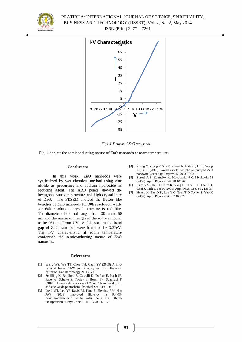
PRATIBHA: INTERNATIONAL JOURNAL OF SCIENCE, SPIRITUALITY,
BUSINESS AND TECHNOLOGY (IJSSBT), Vol. 2, No. 2, May 2014
ISSN (Print) 2277—7261
91
Fig4 .I-V curve of ZnO nanorods
Fig. 4 depicts the semiconducting nature of ZnO nanorods at room temperature.
Conclusion:
In this work, ZnO nanorods were
synthesized by wet chemical method using zinc
nitride as precursors and sodium hydroxide as
reducing agent. The XRD peaks showed the
hexagonal wurtzite structure and high crystallinity
of ZnO. The FESEM showed the flower like
bunches of ZnO nanorods for 30k resolution while
for 60k resolution, crystal structure is rod like.
The diameter of the rod ranges from 30 nm to 60
nm and the maximum length of the rod was found
to be 961nm. From UV- visible spectra the band
gap of ZnO nanorods were found to be 3.37eV.
The I-V characteristic at room temperature
conformed the semiconducting nature of ZnO
nanorods.
References
[1] Wang WS, Wu TT, Chou TH, Chen YY (2009) A ZnO
nanorod based SAW oscillator system for ultraviolet
detection, Nanotechnology 20:135503 [2] Schilling K, Bradford B, Casrelli D, Dufour E, Nash JF,
Pape W, Schulte S, Tooley L, Bosch JV, Schellauf F
(2010) Human safety review of ―nano‖ titanium dioxide and zinc oxide photochem Photobiol Sci 9:495-509
[3] Loyd MT, Lee YJ, Davis RJ, Fang E, Fleming RM, Hsu
JWP (2009) Improved fficiency in Poly(3-hexylthiophene)zinc oxide solar cells via lithium
incorporation. J Phys Chem C 113:17608-17612
[4] Zhang C, Zhang F, Xia T, Kumar N, Hahm J, Liu J, Wang
ZL, Xu J (2009) Low-threshold two photon pumped ZnO nanowire lasers. Opt Express 17:7893-7900
[5] Zuruzi A S, Kolmalov A, Macdonald N C, Moskovits M
(2006) Appl. Physics Lett. 88 102904 [6] Kilm Y.S., Ha S C, Kim K, Yang H, Park J. T., Lee C H,
Choi J, Paek J. Lee K (2005) Appl. Phys. Lett. 86 213105
[7] Huang H, Tan O K, Lee Y C, Tran T D Tse M S, Yao X (2005) Appl. Physics lett. 87 163123
-35
-25
-15
-5
5
15
25
35
45
55
65
75
-30-26-22-18-14-10-6 -2 2 6 10 14 18 22 26 30
I-V Characteristics
I
V
I
V

PRATIBHA: INTERNATIONAL JOURNAL OF SCIENCE, SPIRITUALITY,
BUSINESS AND TECHNOLOGY (IJSSBT), Vol. 2, No. 2, May 2014
ISSN (Print) 2277—7261
92
Effective Employee Engagement Programme to Enhance the
Performance of Employee: A case study of Vivanta by Taj
Blue Diamond, Pune
Dr.Vishal S.Rana 1,Yateen S.Nandanwar
2
1 Asst Prof & Head, M.B.A Dept, S.S.B.T‘s College of Engineering & Technology, Bambhori, Jalgaon,
MS (Corresponding Author) 2 Student (MBA-II), Department of Business Administration, SSBT‘s College of Engineering &
Technology, Bambhori, Jalgaon, MS, India.
Email: [email protected]
Abstract— EmployeeEngagement is about
creating opportunities for employees to connect
with their colleagues, managers and wider
organization. It is also about creating an
environment where employees are motivated to
want to connect with their work and really care
about doing a good job. It is a concept that
places flexibility, change and continuous
improvement at the heart of what it means to
be? Engagement is more than simply
satisfaction or even commitment. Satisfied
employees may be happy but make little
contribution to the organization; yet committed
employees may be focusing on the wrong
objectives. Producing a satisfied and committed
workforce is a worthwhile aim but on its own it
is not enough. This discussion paper is aimed at
senior HR professionals and others who are
considering an employee engagement
framework as part of their effective people
management policies.
Keywords-Employee Engagement Programme,
Training, Employee Motivation, Education
Communication,
I. INTRODUCTION
What motivates people to do a good job? How can
organizations get the best out of their people?
These questions are not new, but today many
employers are answering them with a fresh
conviction and sense of purpose. These employers
are confident they have a practical framework that
helps them build and maintain positive relations
with their workforce. That framework is called
‗Employee Engagement‘.
Engagement is about creating opportunities for
employees to connect with their colleagues,
managers and wider organization. It is also about
creating an environment where employees are
motivated to want to connect with their work and
really care about doing a good job. It is a concept
that places flexibility, change and continuous
improvement at the heart of what it means to be?
Engagement ismore than simply satisfaction
oreven commitment. Satisfied employees may be
happy but make little contribution to the
organization; yet committed employees may be
focusing on the wrong objectives. Producing a
satisfied and committed workforce is a worthwhile
aim but on its own it is not enough. This discussion
paper is aimed at senior HR professionals and
others who are considering an employee
engagement framework as part of their effective
people management policies.
The paper focuses on:
Outlines key elements of the business case
that can help persuade top management of the
contribution engaged employees make to
organizational performance.
Identifies the key factors driving employee
engagement, as well as the possible barriers.
Highlights responsibilities in workplaces for
promoting employee engagement and suggests
what employers and government should do to
create an engaged workforce.
II. OBJECTIVES OF THE PAPER
To focus on various Employee Engagement
practice adopted by Vivanta by Taj Blue
Diamond.
To study training and development
programmed used in Vivanta by Taj Blue
Diamond.
To know how the performance of the
employees is being appraised.
To study employee welfare policies.
To identify the problem areas and submit
reports/suggestions wherever necessary.
III. RESEARCH METHODOLOGY

PRATIBHA: INTERNATIONAL JOURNAL OF SCIENCE, SPIRITUALITY,
BUSINESS AND TECHNOLOGY (IJSSBT), Vol. 2, No. 2, May 2014
ISSN (Print) 2277—7261
93
This paper is mostly prepared with the help of
primary data collection. For the study the primary
data was collected through:-
Interaction with managers and departmental
heads.
Conversation with employees at all levels.
The Questionnaire of employee engagement
program consisted of 16 questions which were
collected from 50 employees. In present study, the
researcher has collected primary data by filling
structured questions from employee through
deliberate sampling method. The primary data was
collected from the respondent (employee) within
organization.
IV. IMPORTANCE OF THE STUDY
Many studies have shown that investments in
people (i.e., HR-related practices) have a reliable
impact on the performance of organizations. The
Bureau of Labor conducted a comprehensive
review of more than 100 studies and found that
people practices have significant relationships to
improvements in productivity, satisfaction, and
financial performance. Research has shown that
when engagement scores are high, employees are
more satisfied, less likely to leave the organization,
and more productive.
Each organization is different and there
are many factors that affect bottom-line outcomes;
however, engagement scores can serve as
meaningful predictors of long-term success. Some
organizations use engagement scores as lead
measures in their HR scorecards. When an
organization can show the relationship between
engagement scores and bottom-line outcomes,
everyone pays attention to the engagement index.
Establishing this critical link between people and
performance helps HR professionals prove that
people-related interventions are a worthwhile
investment.
V. KEY PARAMETERS
Engage Employees early and often: - Ensure
employees have a voice in the program. Ask
employees what question could be asked for a
survey, have them participate in looking at the
results, and give them an opportunity to
generate strategies and interventions. We
won‘t get everyone on the same page unless
we give everyone a hand in authoring that
page.
Focus on Employee Engagement for all: - The
employees should benefit from their
engagement, the organization should see
results, and customers should also experience
the benefits of engaged employees. As you
plan any program ensure you have declarative
clarity on how everyone will benefit.
Get connected: - Join the Employee
Engagement Network. There are over 150
members interested in employee engagement.
Join us to ask questions, find information,
offer support, and stay current on the latest
information in employee engagement. The
glue of engagement is contribution and we
welcome your contribution.
Rewards as to motivate: - The employee
should get the benefits of become Wall of
Fame in terms of money which hotel is not
providing to them.
VI. ANALYSIS OF STUDY
Q.1 Opportunity at Work place through Employee
engagement programme
Chart 1.1
Interpretation:In every month, Hotel organizes
training for their employee for further development
of their knowledge and skill which is indirectly
helpful for organization for achieving the goal. The
above pie chart depicts that in view of 72 %
employee there are opportunities at work place at
Vivanta-Taj Blue Diamond, Pune through
employee engagement programme.
72%
16%12%
Always
Sometime
No
Opportunity at Work

PRATIBHA: INTERNATIONAL JOURNAL OF SCIENCE, SPIRITUALITY,
BUSINESS AND TECHNOLOGY (IJSSBT), Vol. 2, No. 2, May 2014
ISSN (Print) 2277—7261
94
Q.2 Does Employee Engagement Programme
increase the morale of employees
Table 1.1
Interpretation: - From the above table it is found
that 96 % respondents are completely agree that
employee engagement programme enhances the
morale of employee.
Q.3 Employee Recognition/Praise at work place
for doing good work by Taj Blue Diamond
Chart 1.2
Interpretation: From the above pie chart it is
observed that in view of 36 % employees, their
work has always been appraised by Taj Blue
Diamond at work place whereas 24 % employee
felt that their work has sometimes appraised by Taj
Blue Diamond at work place for doing good job.
Q.4 Most suitable employee engagement practice
for increasing the motivation of employee.
Sr.
No
Particulars No.of
Employee
%
1 Cultural Events 10 20 %
2 Sports Week 8 16 %
3 Recreational Tour 12 24 %
4 Annual Gathering 7 14 %
5 Movie Break 6 12 %
6 Festiwal Celebration 4 8 %
7 Wall of Fame 3 6 %
8 Total 50 100
Table 1.2
Interpretation: From the above table it is found that
in view of 24 % employee, recreational tour is the
most suitable employee engagement practice to
motivate the employee whereas 16 % employee
feel that organizing sports week for employee may
motivate them.
Q.5 Rating the effectiveness of employee
engagement practices adopted by Vivanta by Taj
Blue Diamond on 1-5 scale.
Sr.
No
Particulars No.of
Employee
%
1 Poor 3 6 %
2 Average 7 14 %
3 Good 10 20 %
4 Very Good 25 50 %
5 Excellent 5 10 %
6 Total 50 100
Table 1.3
Interpretation: From the above table it is revealed
that the maximum i.e 50 % employee appreciated
the employee engagement practices adopted by
Vivanta by Taj Blue Diamond, Pune whereas in
opinion of 10 % employees the employee
engagement practices of Vivanta by Taj is
excellent.
VII. FINDINGS
It was concluded that most of employee feels
that their supervisor take care of their and also
taking feedback about their work and taking
suggestions from them to increase the
efficiency of employee. But few of the
employee opinions are opposite to this they
think so that their supervisor does not take
care of their.
The question was asked to employee that is
their opinions which they have given to their
supervisor are counted or not. The majority of
the employee says that sometimes their
opinions are counted by supervisors.
It was revealed that, within organization
employees are having best friend. The reason
behind this is the activity which the hotel
using to engage the employee and making
them free with their colleague, peers and with
supervisors. Very few employees were newly
joined the hotel and having few friends at
work place.
Most of the employee got an opportunity to do
their best every day in the organization.
Because of freely atmosphere and culture in
the hotel the employee feels that their opinions
and suggestions are counted by the supervisors
and with this they feels opportunity to grow.
But few are not satisfied with this statement as
we can see in the bar chart some respondents
Sr.
No
Particulars No. of
Respondents
Percentage
1 Yes 48 96%
2 No 2 4%
3 Total 50 100%

PRATIBHA: INTERNATIONAL JOURNAL OF SCIENCE, SPIRITUALITY,
BUSINESS AND TECHNOLOGY (IJSSBT), Vol. 2, No. 2, May 2014
ISSN (Print) 2277—7261
95
feel little bit opportunity. Rest equal number
of employee feel little bit and some does not.
Disclosure of the study shows that, the
respondents are very confused while choosing
the option. Few employees want to select the
entire options which have been provided to
them. But from the analysis of the data,
researcher found that most of the employees
like the recreational tour a lot because they got
different experience outside the hotel premises
and follow with the cultural event which
includes celebration of each festivals, sports
week and annual gathering. The very less have
selected wall of fame because they feel this is
the Non-financial motivational schemewhich
hotel are using for motivation of employee
and for this lots of efforts they need to give
along with work.
Finally the researcher asked the overall rating
about engagement practices which the hotel is
carried out are well acceptable by the
employee and make them happy while doing
their job. Most of the employee marks V.
Good because of good experience which they
have got while participating in such events.
Few of the employee stated as excellent which
are completely satisfied and few has stated
poor because of not participating in activities.
CONCLUSION
After taking the feedback from the employees,
it is observed that they are hardworking and
dedicated towards their work. But a number of
employees are not interested in schemes such
as Wall of Fame and programs organized by
the management of the organization. For Wall
of Fame which is less likely by employee can
be seen after analyzing the feedback which
they have filled. The major reason behind this
activity is Non Financial type of motivation
which organization is providing and also a lot
of efforts they need to give to achieve it.
During the research, researcher has noticed
that some of the employees are illiterate and
they want to participate but they cannot
because of less confident and less motivated.
Employees want more facilities from
managements such as gifts, incentives, bonus
etc. when they participate in various programs
and company also work on these ways to
encourage their employees.
REFERENCES
[1]. Human Resource Management by K.Ashwathappa – Tata
McGrawHill
[2]. Human Resource Management by S.S.Khanka; S. Chand
& Co.ltd. New Delhi. [3]. Taj Group Magazines Oct 2009.
[4]. Essential of HRM and Industrial Relations by P.Subha
Rao – Himalaya Publications. [5]. Human Resource Management By Dr. C.B. Gupta –
Sultan Chand & Sons
[6]. HR Magazines [7]. www.google.com
[8]. http://www.vivantabytaj.com/Blue-Diamond-
Pune/Promotions.aspx\
