volume 2 issue 3 september 2018
TRANSCRIPT
VOLUME 2 ISSUE 3 SEPTEMBER 2018
ISSN 2587-1366
EDITOR IN CHIEF
Prof. Dr. Murat YAKAR
Mersin University Engineering Faculty
Turkey
CO-EDITORS
Prof. Dr. Erol YAŞAR
Mersin University Faculty of Art and Science
Turkey
Assoc. Prof. Dr. Cahit BİLİM
Mersin University Engineering Faculty
Turkey
Assist. Prof. Dr. Hüdaverdi ARSLAN
Mersin University Engineering Faculty
Turkey
ADVISORY BOARD
Prof. Dr. Orhan ALTAN
Honorary Member of ISPRS, ICSU EB Member
Turkey
Prof. Dr. Armin GRUEN
ETH Zurih University
Switzerland
Prof. Dr. Hacı Murat YILMAZ
Aksaray University Engineering Faculty
Turkey
Prof. Dr. Artu ELLMANN
Tallinn University of Technology Faculty of Civil Engineering
Estonia
Assoc. Prof. Dr. E. Cağlan KUMBUR
Drexel University
USA
TECHNICAL EDITORS
Prof. Dr. Ali AKDAĞLI
Dean of Engineering Faculty
Turkey
Prof. Dr. Roman KOCH
Erlangen-Nurnberg Institute Palaontologie
Germany
Prof. Dr. Hamdalla WANAS
Menoufyia University, Science Faculty
Egypt
Prof. Dr. Turgay CELIK
Witwatersrand University
South Africa
Prof. Dr. Muhsin EREN
Mersin University Engineering Faculty
Turkey
Prof. Dr. Johannes Van LEEUWEN
Iowa State University
USA
Prof. Dr. Elias STATHATOS
TEI of Western Greece
Greece
Prof. Dr. Vedamanickam SAMPATH
Institute of Technology Madras
India
Prof. Dr. Khandaker M. Anwar HOSSAIN
Ryerson University
Canada
Prof. Dr. Hamza EROL
Mersin University Engineering Faculty
Turkey
Prof. Dr. Ali Cemal BENIM
Duesseldorf University of Aplied Sciences
Germany
Prof. Dr. Mohammad Mehdi RASHIDI
University of Birmingham
England
Prof. Dr. Muthana SHANSAL
Baghdad University
Iraq
Prof. Dr. Ibrahim S. YAHIA
Ain Shams University
Egypt
Assoc. Prof. Dr. Kurt A. ROSENTRATER
Iowa State University
USA
Assoc. Prof. Dr. Christo ANANTH
Francis Xavier Engineering College
India
Assoc. Prof. Dr. Bahadır K. KÖRBAHTİ
Mersin University Engineering Faculty
Turkey
Assist. Prof. Dr. Akın TATOGLU
Hartford University College of Engineering
USA
Assist. Prof. Dr. Şevket DEMİRCİ
Mersin University Engineering Faculty
Turkey
Assist. Prof. Dr. Yelda TURKAN
Oregon State University
USA
Assist. Prof. Dr. Gökhan ARSLAN
Mersin University Engineering Faculty
Turkey
Assist. Prof. Dr. Seval Hale GÜLER
Mersin University Engineering Faculty
Turkey
Assist. Prof. Dr. Mehmet ACI
Mersin University Engineering Faculty
Turkey
Dr. Ghazi DROUBI
Robert Gordon University Engineering Faculty
Scotland, UK
JOURNAL SECRETARY
Nida DEMİRTAŞ
TURKISH JOURNAL OF ENGINEERING (TUJE)
Turkish Journal of Engineering (TUJE) is a multi-disciplinary journal. The Turkish Journal of Engineering (TUJE) publishes
the articles in English and is being published 3 times (January, May, September) a year. The Journal is a multidisciplinary
journal and covers all fields of basic science and engineering. It is the main purpose of the Journal that to convey the latest
development on the science and technology towards the related scientists and to the readers. The Journal is also involved in
both experimental and theoretical studies on the subject area of basic science and engineering. Submission of an article implies
that the work described has not been published previously and it is not under consideration for publication elsewhere. The
copyright release form must be signed by the corresponding author on behalf of all authors. All the responsibilities for the
article belongs to the authors. The publications of papers are selected through double peer reviewed to ensure originality,
relevance and readability.
AIM AND SCOPE
The Journal publishes both experimental and theoretical studies which are reviewed by at least two scientists and researchers
for the subject area of basic science and engineering in the fields listed below:
Aerospace Engineering
Environmental Engineering
Civil Engineering
Geomatic Engineering
Mechanical Engineering
Geology Science and Engineering
Mining Engineering
Chemical Engineering
Metallurgical and Materials Engineering
Electrical and Electronics Engineering
Mathematical Applications in Engineering
Computer Engineering
Food Engineering
PEER REVIEW PROCESS
All submissions will be scanned by iThenticate® to prevent plagiarism. Author(s) of the present study and the article about the
ethical responsibilities that fit PUBLICATION ETHICS agree. Each author is responsible for the content of the article. Articles
submitted for publication are priorly controlled via iThenticate ® (Professional Plagiarism Prevention) program. If articles that
are controlled by iThenticate® program identified as plagiarism or self-plagiarism with more than 25% manuscript will return
to the author for appropriate citation and correction. All submitted manuscripts are read by the editorial staff. To save time for
authors and peer-reviewers, only those papers that seem most likely to meet our editorial criteria are sent for formal review.
Reviewer selection is critical to the publication process, and we base our choice on many factors, including expertise,
reputation, specific recommendations and our own previous experience of a reviewer's characteristics. For instance, we avoid
using people who are slow, careless or do not provide reasoning for their views, whether harsh or lenient. All submissions will
be double blind peer reviewed. All papers are expected to have original content. They should not have been previously
published and it should not be under review. Prior to the sending out to referees, editors check that the paper aim and scope of
the journal. The journal seeks minimum three independent referees. All submissions are subject to a double blind peer review;
if two of referees gives a negative feedback on a paper, the paper is being rejected. If two of referees gives a positive feedback
on a paper and one referee negative, the editor can decide whether accept or reject. All submitted papers and referee reports are
archived by journal Submissions whether they are published or not are not returned. Authors who want to give up publishing
their paper in TUJE after the submission have to apply to the editorial board in written. Authors are responsible from the writing
quality of their papers. TUJE journal will not pay any copyright fee to authors. A signed Copyright Assignment Form has to
be submitted together with the paper.

PUBLICATION ETHICS
Our publication ethics and publication malpractice statement is mainly based on the Code of Conduct and Best-Practice
Guidelines for Journal Editors. Committee on Publication Ethics (COPE). (2011, March 7). Code of Conduct and Best-Practice
Guidelines for Journal Editors. Retrieved from http://publicationethics.org/files/Code%20of%20Conduct_2.pdf
PUBLICATION FREQUENCY
The TUJE accepts the articles in English and is being published 3 times. January, May, September a year.
CORRESPONDENCE ADDRESS
Journal Contact: [email protected]
CONTENTS Volume 2 – Issue 3
ARTICLES
RHEOLOGICAL PARAMETER ESTIMATION OF CMC-WATER SOLUTIONS USING MAGNETIC
RESONANCE IMAGING (MRI)
G. Bengusu Tezel ....................................................................................................................................................................... 94
INVESTIGATION OF Ni-Mn BASED SHAPE MEMORY ALLOY VARIATIONS TRANSFORMATION
TEMPERATURES
Ece Kalay, Anıl Erdağ Nomer and Mehmet Ali Kurgun ............................................................................................................ 98
INVESTIGATION OF DISSOLUTION KINETICS OF Zn AND Mn FROM SPENT ZINC-CARBON BATTERIES
IN SULPHURIC ACID SOLUTION
Tevfik Agacayak and Ali Aras ................................................................................................................................................. 107
COMPARATIVE STUDY OF REGIONAL CRASH DATA IN TURKEY
Murat Özen.............................................................................................................................................................................. 113
PERFORMANCE COMPARISON OF ANFIS, ANN, SVR, CART AND MLR TECHNIQUES FOR GEOMETRY
OPTIMIZATION OF CARBON NANOTUBES USING CASTEP
Mehmet Acı, Çiğdem İnan Acı and Mutlu Avcı ....................................................................................................................... 119
INVESTIGATION OF ULEXITE USAGE IN AUTOMOTIVE BRAKE FRICTION MATERIALS
Banu Sugözü ............................................................................................................................................................................ 125
CRITICALITY CALCULATION OF A HOMOGENOUS CYLINDRICAL NUCLEAR REACTOR CORE USING
FOUR-GROUP DIFFUSION EQUATIONS
Babatunde Michael Ojo, Musibau Keulere Fasasi, Ayodeji Olalekan Salau, Stephen Friday Olukotun and Ademola Mathew
Jayeola .................................................................................................................................................................................... 130

Turkish Journal of Engineering
94
Turkish Journal of Engineering (TUJE)
Vol. 2, Issue 3, pp. 94-97, September 2018
ISSN 2587-1366, Turkey
DOI: 10.31127/tuje.363596
Research Article
RHEOLOGICAL PARAMETER ESTIMATION OF CMC-WATER SOLUTIONS
USING MAGNETIC RESONANCE IMAGING (MRI)
G. Bengusu Tezel *1
1 Abant Izzet Baysal University, Faculty of Engineering and Architecture, Department of Chemical Engineering,
Bolu, Turkey
ORCID ID 0000-0002-0671-208X
* Corresponding Author
Received: 07/12/2017 Accepted: 20/01/2018
ABSTRACT
In this study, the application of Magnetic Resonance Imaging (MRI) rheometry on the measurement of complex fluid
Carboxylmethyl cellulose (CMC)-water solutions (0.5%, 1.0%, 1.5%, 2.0% w/w) flow was described. Depending on
CMC concentration, Power law or Herschel-Bulkley models gave the best fit according to MRI and conventional
rheometer (CVO) results. Power Law model was valid for 0.5% and 1.0% CMC (R2=0.9993-R2=0.9987 and R2=0.9983-
R2=0.9985 respectively by MRI and CVO). On the other hand, 1.5% and 2.0% CMC solutions flow were well described
by Herschel–Bulkley model (R2=0.9994-R2=0.9996 and R2=0.9986-R2=0.9981 respectively by MRI and CVO). The MRI
measurements agreed well with the CVO measurements.
Keywords: Magnetic Resonance Imaging, Conventional Rheometer, CMC, Rheology

Turkish Journal of Engineering (TUJE)
Vol. 2, Issue 3, pp. 94-97, September 2018
95
1. INTRODUCTION
Offline methods for rheological measurements such
as cylindirical coquette, cone and plate geometries
(conventional rheometries) generally used for the study
of fluid motion in shear. However, obtained results
from these types of geometries need to be verified with
suitable online or inline methods. Especially, many
industrial processes, such as extrusion, transfer
processes involve established or developing flows in
pipes or tubes. Therefore, online techniques based on the
measurement of the velocity profile in a pipe flow using
Magnetic Resonance Imaging (MRI), which is a non-
invasive method, and simultaneously determining the
pressure drop, are promising for use a product quality or
rheology control tool during the fluid flow. Magnetic
resonance imaging (MRI) can be used as a viscometer,
based on analysis of a measured velocity profile of fluid
flowing in a tube coupled with a simultaneous
measurement of the pressure drop driving the flow
(Arola et al., 1997 and Arola et al., 1999).
This type of measurement is well suited for rheological
characterization of non-Newtonian fluids (Choi et al.,
2002 and Tozzi et al., 2012).
To evaluate shear viscosity in tube (or capillary)
flow, an incompressible fluid must undergo steady
pressure-driven flow in the laminar regime. The
conservation of linear momentum, which equates
pressure forces to viscous forces, provides the
relationship between the shear stress, σ, and radial
position, r:
𝜎(𝑟) =−𝛥𝑃
2𝐿𝑟
where ΔP is the pressure drop over the tube length L.
The shear rate is obtained at the same radial position
using the velocity profile obtained from a flow image.
The expression for the shear rate in tube flow is:
𝛾(𝑟) =𝑑𝑉(𝑟)
𝑑𝑟
Where V is the axial velocity. Using Equations 2
and 3, the apparent viscosity η is determined by the ratio
of shear stress to shear rate:
𝜂(𝑟) =𝜎(𝑟)
𝛾(𝑟)
Graphical User Interface (GUI) programs are used to
analyze data and display rheological results (Choi et al.,
2005 and Tozzi et al., 2012). Main step in the data
processing procedure include calculating the shear stress
as a function of radial position in the pipe, processing
the velocity profile image to obtain a velocity profile,
calculating the shear rate as a function of radial position
from the velocity profile, and generating the rheogram
by plotting the shear stress against the shear rate (Arola
et al., 1997, Callaghan 1999 and Tozzi et al., 2012).
Calculating the shear stress is straightforward as in
Equation 1.
In this study, Carboxymethyl cellulose (CMC) was
used as test fluid. CMC is widely used as thickener
especially in food and pharmaceutical industries
(Benchabane and Bekkour, 2008). This is also known as
complex fluid due to no linear relationship between
stress and shear rate in simple shear during the flow.
2. MATERIALS AND METHODS
2.1. Materials
The CMC, with nominal molecular weight of
250,000 g/mol was supplied from Sigma. Aqueous
solutions of CMC were prepared by dissolving the
appropriate amount of CMC powder in distilled water.
The high CMC concentration solutions (0.5%, 1.0%,
1.5%, 2% w/w.) were prepared by using water heated at
50 oC by gentle stirring with the sufficient time < 24 h.
Online and offline measurements were performed
with an MRI (Magnetic Resonance Imaging) at Food
and Science Technology Department at University of
California, Davis, USA using flow loop depicted in Fig.
1. At 25 oC, MRI Flow Imaging Tests were done for 0.5,
1, 1.5, 2% (w/w) CMC solutions to determine
rheological constitutive equations parameters. Inlet
diamater of PVC tube was 38.1 mm. The test fluid was
recirculated using Moyno pump (Integrated Motor Drive
System, Franklin Electric) Pressure drop was obtained at
the ends of pipe with a constant length of 1.68 m using
pressure transducer (Siemens Company).
Fig. 1. Flow loop setup for CMC testing A) Positive
displacement pump B) MRI magnet
2.2. Methods
In Fig. 2, flow image for an example of 0.5% CMC
flow, can be seen with data processing window. The
velocity profile is used to obtain shear rate distribution,
while the pressure drop is used to calculate the shear
stress distribution. By taking the ratio of these quantities
at a radial position, local viscosity can be obtained
within the shear rate range in the flow, zero at the center,
and maximum at the wall, within minutes. There is not
observed slip effect on the wall as in Fig. 2.
Fig. 2. MRI Image for 0.5% CMC
(1)
(2)
(3)
(1)
Turkish Journal of Engineering (TUJE)
Vol. 2, Issue 3, pp. 94-97, September 2018
96
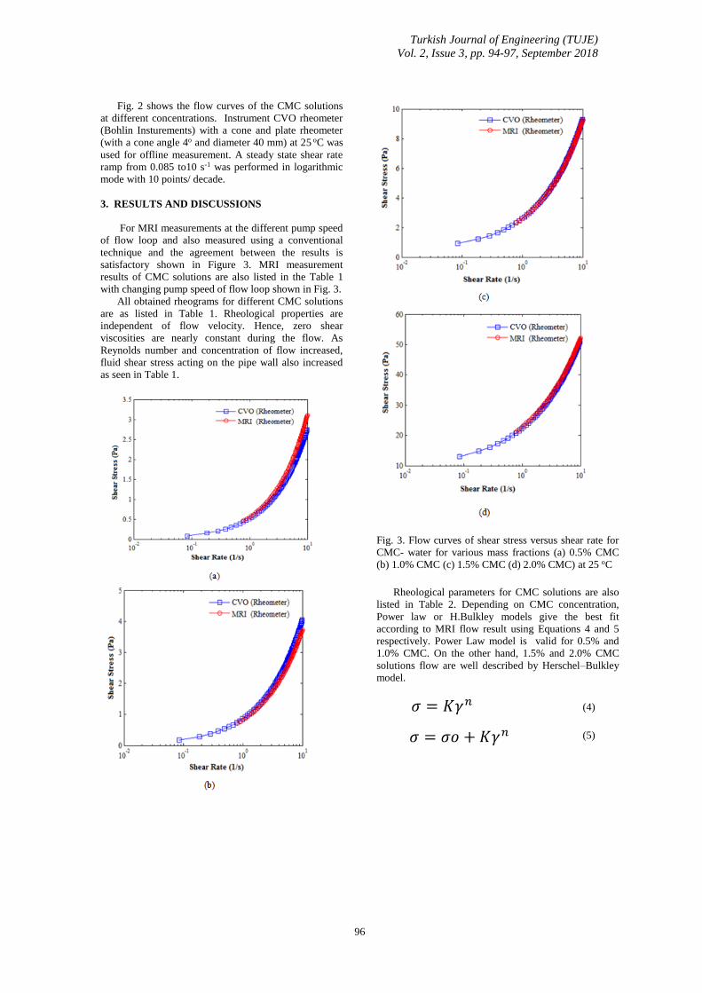
Fig. 2 shows the flow curves of the CMC solutions
at different concentrations. Instrument CVO rheometer
(Bohlin Insturements) with a cone and plate rheometer
(with a cone angle 4o and diameter 40 mm) at 25 oC was
used for offline measurement. A steady state shear rate
ramp from 0.085 to10 s-1 was performed in logarithmic
mode with 10 points/ decade.
3. RESULTS AND DISCUSSIONS
For MRI measurements at the different pump speed
of flow loop and also measured using a conventional
technique and the agreement between the results is
satisfactory shown in Figure 3. MRI measurement
results of CMC solutions are also listed in the Table 1
with changing pump speed of flow loop shown in Fig. 3.
All obtained rheograms for different CMC solutions
are as listed in Table 1. Rheological properties are
independent of flow velocity. Hence, zero shear
viscosities are nearly constant during the flow. As
Reynolds number and concentration of flow increased,
fluid shear stress acting on the pipe wall also increased
as seen in Table 1.
Fig. 3. Flow curves of shear stress versus shear rate for
CMC- water for various mass fractions (a) 0.5% CMC
(b) 1.0% CMC (c) 1.5% CMC (d) 2.0% CMC) at 25 oC
Rheological parameters for CMC solutions are also
listed in Table 2. Depending on CMC concentration,
Power law or H.Bulkley models give the best fit
according to MRI flow result using Equations 4 and 5
respectively. Power Law model is valid for 0.5% and
1.0% CMC. On the other hand, 1.5% and 2.0% CMC
solutions flow are well described by Herschel–Bulkley
model.
𝜎 = 𝐾𝛾𝑛
𝜎 = 𝜎𝑜 + 𝐾𝛾𝑛
(4)
(5)
Turkish Journal of Engineering (TUJE)
Vol. 2, Issue 3, pp. 94-97, September 2018
97
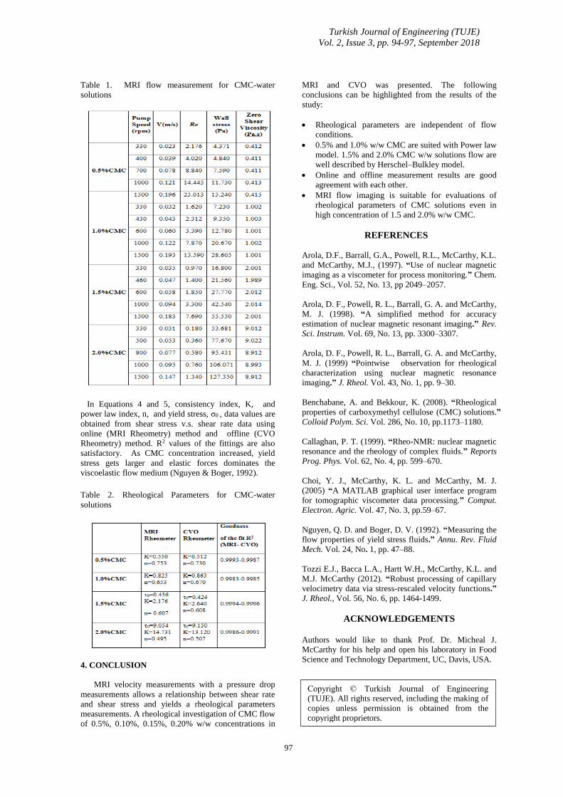
Table 1. MRI flow measurement for CMC-water
solutions
In Equations 4 and 5, consistency index, K, and
power law index, n, and yield stress, σ0 , data values are
obtained from shear stress v.s. shear rate data using
online (MRI Rheometry) method and offline (CVO
Rheometry) method. R2 values of the fittings are also
satisfactory. As CMC concentration increased, yield
stress gets larger and elastic forces dominates the
viscoelastic flow medium (Nguyen & Boger, 1992).
Table 2. Rheological Parameters for CMC-water
solutions
4. CONCLUSION
MRI velocity measurements with a pressure drop
measurements allows a relationship between shear rate
and shear stress and yields a rheological parameters
measurements. A rheological investigation of CMC flow
of 0.5%, 0.10%, 0.15%, 0.20% w/w concentrations in
MRI and CVO was presented. The following
conclusions can be highlighted from the results of the
study:
Rheological parameters are independent of flow
conditions.
0.5% and 1.0% w/w CMC are suited with Power law
model. 1.5% and 2.0% CMC w/w solutions flow are
well described by Herschel–Bulkley model.
Online and offline measurement results are good
agreement with each other.
MRI flow imaging is suitable for evaluations of
rheological parameters of CMC solutions even in
high concentration of 1.5 and 2.0% w/w CMC.
REFERENCES
Arola, D.F., Barrall, G.A., Powell, R.L., McCarthy, K.L.
and McCarthy, M.J., (1997). “Use of nuclear magnetic
imaging as a viscometer for process monitoring.” Chem.
Eng. Sci., Vol. 52, No. 13, pp 2049–2057.
Arola, D. F., Powell, R. L., Barrall, G. A. and McCarthy,
M. J. (1998). “A simplified method for accuracy
estimation of nuclear magnetic resonant imaging.” Rev.
Sci. Instrum. Vol. 69, No. 13, pp. 3300–3307.
Arola, D. F., Powell, R. L., Barrall, G. A. and McCarthy,
M. J. (1999) “Pointwise observation for rheological
characterization using nuclear magnetic resonance
imaging.” J. Rheol. Vol. 43, No. 1, pp. 9–30.
Benchabane, A. and Bekkour, K. (2008). “Rheological
properties of carboxymethyl cellulose (CMC) solutions.”
Colloid Polym. Sci. Vol. 286, No. 10, pp.1173–1180.
Callaghan, P. T. (1999). “Rheo-NMR: nuclear magnetic
resonance and the rheology of complex fluids.” Reports
Prog. Phys. Vol. 62, No. 4, pp. 599–670.
Choi, Y. J., McCarthy, K. L. and McCarthy, M. J.
(2005) “A MATLAB graphical user interface program
for tomographic viscometer data processing.” Comput.
Electron. Agric. Vol. 47, No. 3, pp.59–67.
Nguyen, Q. D. and Boger, D. V. (1992). “Measuring the
flow properties of yield stress fluids.” Annu. Rev. Fluid
Mech. Vol. 24, No. 1, pp. 47–88.
Tozzi E.J., Bacca L.A., Hartt W.H., McCarthy, K.L. and
M.J. McCarthy (2012). “Robust processing of capillary
velocimetry data via stress-rescaled velocity functions.”
J. Rheol., Vol. 56, No. 6, pp. 1464-1499.
ACKNOWLEDGEMENTS
Authors would like to thank Prof. Dr. Micheal J.
McCarthy for his help and open his laboratory in Food
Science and Technology Department, UC, Davis, USA.
Copyright © Turkish Journal of Engineering
(TUJE). All rights reserved, including the making of
copies unless permission is obtained from the
copyright proprietors.

Turkish Journal of Engineering
98
Turkish Journal of Engineering (TUJE)
Vol. 2, Issue 3, pp. 98-106, September 2018
ISSN 2587-1366, Turkey
DOI: 10.31127/tuje.374215
Research Article
INVESTIGATION OF Ni-Mn BASED SHAPE MEMORY ALLOY VARIATIONS
TRANSFORMATION TEMPERATURES
Ece Kalay *1, Anıl Erdağ Nomer 2 and Mehmet Ali Kurgun 3
1 Mersin University, Engineering Faculty, Department of Mechanical Engineering, Mersin, Turkey
ORCID ID 0000-0003-2470-7791
2 Mersin University, Engineering Faculty, Department of Mechanical Engineering, Mersin, Turkey
ORCID ID 0000 – 0002 – 8997 – 6936
3 Mersin University, Engineering Faculty, Department of Mechanical Engineering, Mersin, Turkey
ORCID ID 0000 – 0001 – 5565 – 1351
* Corresponding Author
Received: 03/01/2018 Accepted: 25/02/2018
ABSTRACT
Shape memory alloys’ usage frequency and areas are increased day to day. It is seen the different type and different
characteristics in many industrial areas. Therefore, shape memory alloys, which are intelligent materials, are very fast to
develop. The NiTi alloys, from these alloy types, are most commonly used due to their low hysteresis range and
biocompatibility. But production costs and difficulties have led, investigators to investigate different alloy types. Shape
memory alloys which produced with possibly cheaper elements, examined in researchers with looking at their
transformation temperatures.
Keywords: Dsc, NiTi, Shape Memory Alloys

Turkish Journal of Engineering (TUJE)
Vol. 2, Issue 3, pp. 98-106, September 2018
99
1. INTRODUCTION
Shape memory alloys (SMA) are materials known as
intelligent metals from the past to present day. In the past,
SMA’s found in various composition ratios of
constrained elements are alloyed with many elemental
ingredients now (Canbay, 2017). SMA’s shed light on
future systems and applications at a high level. The
technologies that will be developed with unique features
will provide great advantages and their usage will be
necessary. High strength, biocompatibility, high wear
resistance, high corrosion resistance, working in high
temperature and pressure, elasticity ductility etc.
intelligent metal alloys are made depending on the needs
of the sectors. Healthcare field, defense, and military
fields, mechanical systems, automotive sectors etc.
(Canbay et al., 2014; Canbay, 2017; Canbay et al., 2017;
Canbay et al., 2018). SMA’s are required to be developed
and used in the fields. Producing SMA’s according to the
needs of the areas to be used will be the best course of
approachment. In order to meet the requirements of the
application areas of SMA materials, the alloys must be
full-featured and very diverse. Once the SMA’s are
approached, technology and sectors will be advantageous
and the work on these intelligent materials will become
more important. The SMA’s are a very valuable issue for
the Research & Development area. Considering the
advantages and convenience of intelligent materials, it is
a bright field of materials that many industries in the
manufacturing and the business world will not spare their
investments and supports (Eskil et al., 2015). SMA's have
a certain high temperature phase and low temperature
phase according to their element proportion that they
contain. The high temperature phase is called the
austenite phase, the low temperature phase is called the
martensite phase. According to the phase temperature
limits, it is determined at which temperature degree the
shape memory conversion. This phase change is due to
solid-state phase change. In general, the memory-trained
shape will talk about memory formation; The SMA
material is subjected to shape training. This is another
issue that needs to be addressed in more detail (Ozkul et
al., 2017). However, in the rough description of the work,
the shape desired to be taken into memory is usually
placed in a mold and heated to a high temperature
austenite phase under tension. The alloyed material is
converted to the low temperature martensite phase by
shock cooling after heating to the austenite phase (Aldas
et al., 2014). This cycle is repeated according to the type
of material and the methods have differed one-way or
two-way. After this process, the SMA will save it in the
memory, which is determined in advance of the applied
processes. After this step, heat, stress, or both subjected
to the plastic deformation that has been exposed and the
shape changes back to the SMA as it was recorded in the
memory when heated from high to the high temperature
austenite phase. It takes its place in the group of
intelligent materials (Canbay et al., 2014). It has been
stated that the SHA’s have various advantageous
properties according to the proportion of the elements
they contain. Today, many test and screening systems are
used in determining these properties. The most common
of these is the differential scanning calorimetry (DSC).
The DSC test is an important test for determining the
temperature points and boundaries of the austenite and
martensite phases, which are very important in the
memory acquisition of SMA’s. The results of DSC
scanning of various alloys of elements such as nickel,
manganese, gallium, iron, aluminum, and tin have been
examined in the literature review. The start and finish
temperatures of the austenite and martensite phases were
determined. The effect of element contents on phase
transformation temperatures was investigated (Aldas et
al., 2016).
The austenite-initiation temperature (As) is the
temperature at which this transformation begins, and the
austenite-final temperature (Af) is the temperature at
which this transformation is complete. When the SMA
heats up, the contract starts and returns to its original
state. This conversion is possible even at high applied
loads and, therefore, results in a high energy density of
the trigger. During the cooling process, the
transformation starts at the martensite starting
temperature (Ms) and completes when the martensite
reaches the finishing temperature (Mf) (Buehler et al.,
1963). Martensite is called the highest temperature Md
that can be caused by residual stress, and when it is above
this temperature, SMA permanently deforms like
ordinary metallic materials (Duerig et al., 1994). These
deforming effects, known as SMA and pseudo elasticity
(or super elasticity), can be categorized according to
three-dimensional memory properties:
One-way shape memory effect (OWSME): The
unidirectional SMA (SMA) maintains a deformed
condition after removing an external force and then
returns to its original state upon heating.
Two-way shape memory effect (TWSME) or
reversible SME: In addition to the one-sided effect,
bi-directional SMA (TWSMA) can remember both
high and low temperature shape. Often the recovery
provided by OWSMA for the same material
(Schroeder et al., 1977; Huang et al., 2000) yields
about half of the water, and this stress tends to
deteriorate quickly, especially at high temperatures
(Ma et al., 2010). For this reason, OWSMA offers a
more reliable and economical solution (Stöckel
1995).
Pseudo elasticity (PE) or Super elasticity (SE): The
SMA returns to its original shape after applying the
mechanical load without the need for any thermal
activation at temperatures between Af and Md.
In addition to the TWSME material above, the
prejudicial OWSMA actuator can also function as a
'mechanical TWSME' at a macroscopic (structural) level;
more robust, reliable, and widely applied in many
engineering applications (Sun et al., 2012). This feature
is important and should be considered carefully when
selecting SMA materials for targeted applications. For
example, a small hysteresis is needed for applications
where rapid movement is necessary (robotic applications)
(Liu, 2010). The physical and mechanical properties of
some SMAs also vary between these two phases, such as
Young's modulus, electrical resistance, thermal
conductivity, and thermal expansion coefficient
(Mihálcz, 2001; Mertmann et al., 2008; Sreekumar et al.,
2009). The austenite structure is rigid and has a high
Young's modulus. The martensite structure is softer. It
can easily deform with the external load (Hodgson et al.,
1990; Mihálcz, 2001).
There are three varieties of SMA. These alloys are
listed in the literature as NiTi, copper based and iron
Turkish Journal of Engineering (TUJE)
Vol. 2, Issue 3, pp. 98-106, September 2018
100
based. The most capable of these alloy types is NiTi
alloys. Because these alloy types have biocompatibility,
they are used in many fields, especially in the field of
medicine. Copper-based SMA is the closest to this type
of alloy. But there is no popular. Iron-based SHA is the
weakest type in this group because they have high
hysteresis. In our study, the data of alloy types which may
be alternative to NiTi-based SMA will be examined. The
temperature transformation points of the austenite and
martensite phases of the samples were determined and
analyzed on the table and the thermal properties of the
shape memory alloys were obtained. All text should be
left and right justified. Footnotes and underlines are not
allowed.
2. LITERATURE REVIEW
The starting and ending temperatures of the austenite
high temperature phase and the martensite low
temperature phase are determined and tabulated in the
literature review. The bibliographic numbers of the
literature search of the thermal values of SMA’s are listed
at the beginning of the table as (Kainuma et al., 1996;
Jiang et al., 2002; Jiang et al., 2003; Wu et al., 2003;
Koho et al., 2004; Lanska et al., 2004; Glavatskyy et al.,
2006; Koyama et al., 2006; Babita et al., 2007; Santos et
al., 2008; Aksoy et al., 2009; Wu et al., 2011; Zheng et
al., 2011; Turabi et al., 2016; Caputo et al., 2017;
Mostafaei et al., 2017). The transformation temperatures
obtained by different element contributions of Ni and Mn-
based SMA materials are shown in Table 1.
2.1. Evaluation of Literature Review
In the direction of information from the source if we
evaluate the change of austenite and martensite starting
end temperature points by changing atomic ratios of
nickel, manganese and aluminum elements, In the first
sample, nickel and manganese were alloyed at 50 percent
and specific temperature points were obtained. It has been
observed that the austenite and martensite phase change
temperatures are lowered when aluminum is added to this
alloy and the manganese proportion is reduced (with the
nickel ratio being kept constant). It is observed that when
the aluminum ratio is kept constant and the nickel ratio is
increased and the manganese ratio is decreased, the phase
change temperatures are increased (Kainuma et al., 1996).
Increasing the tin ratio in nickel, manganese and tin
alloys has clearly reduced the phase conversion
temperature (Koyama et al., 2006; Santos et al., 2008;
Zheng et al., 2011; Turabi et al., 2016).
Nickel, manganese and antimony triple alloys have
been investigated, and when the antimony ratio in the
alloy is reduced, the transformation temperatures of the
austenite and martensite phases have increased at a high
rate. As a result of this observation, antimony addition
reduces the high conversion temperatures (Aksoy et al.,
2009).
Nickel, manganese, and gallium ternary alloys were
added to the dysprosium element and the effects on the
temperature values were observed. When the dysprosium
element increased, the phase transformation temperatures
increased (Babita et al., 2007).
Nickel, manganese, gallium triple alloy system is
added to the silicium element. As the silicium ratio
increased, the phase transformation temperatures
decreased. When cobalt element is added instead of
silicium, cobaltite phase transformation temperatures are
lowered in the same way and the austenite and martensite
start-finish transformation temperatures are increased by
increasing the nickel ratio (Glavatskyy et al., 2006).
Turkish Journal of Engineering (TUJE)
Vol. 2, Issue 3, pp. 98-106, September 2018
101
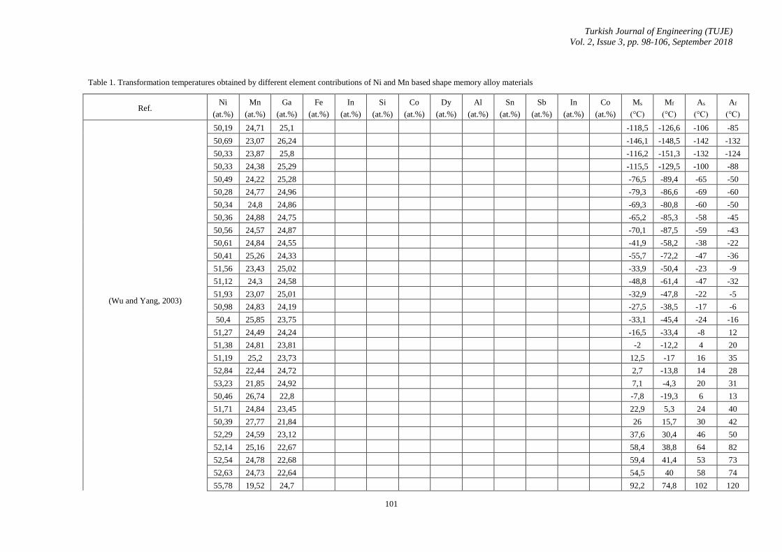
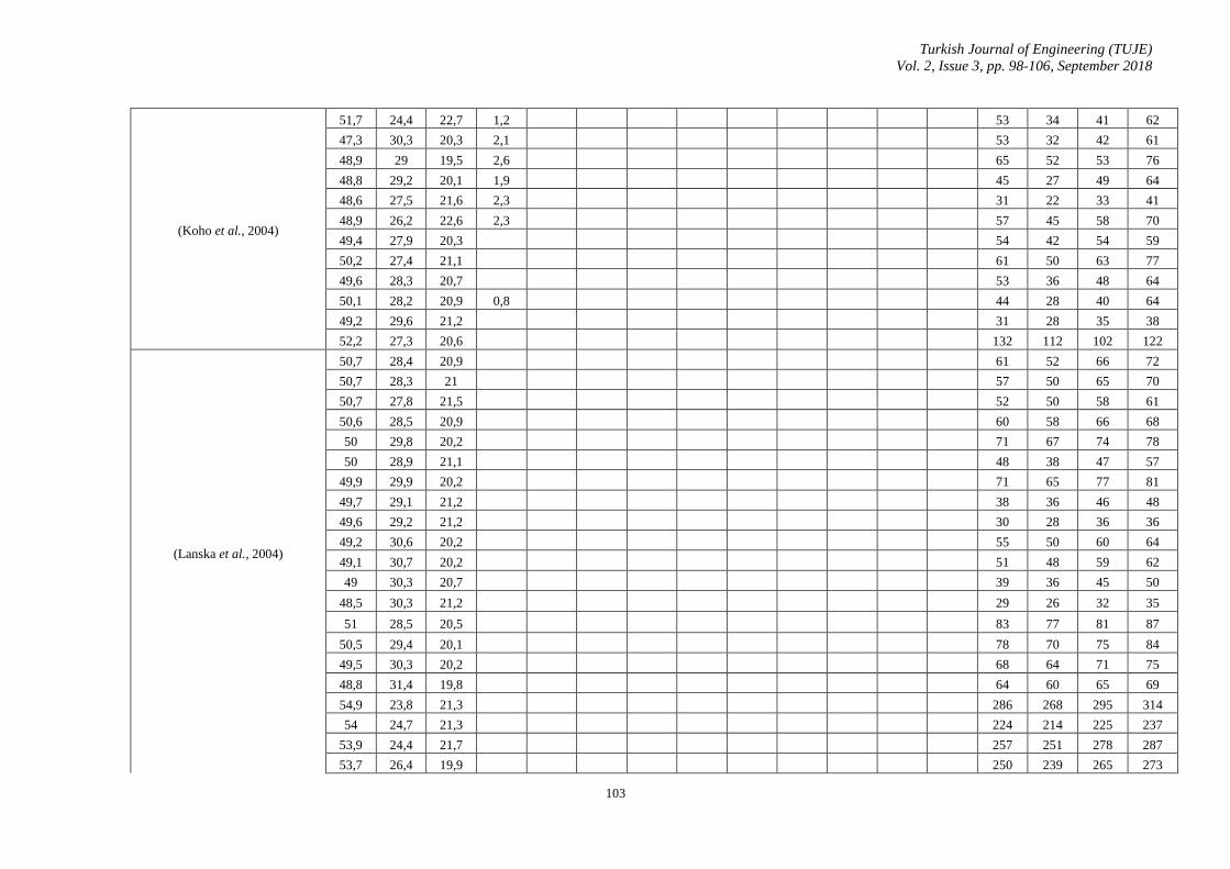
Table 1. Transformation temperatures obtained by different element contributions of Ni and Mn based shape memory alloy materials
Ref. Ni
(at.%)
Mn
(at.%)
Ga
(at.%)
Fe
(at.%)
In
(at.%)
Si
(at.%)
Co
(at.%)
Dy
(at.%)
Al
(at.%)
Sn
(at.%)
Sb
(at.%)
In
(at.%)
Co
(at.%)
Ms
(°C)
Mf
(°C)
As
(°C)
Af
(°C)
(Wu and Yang, 2003)
50,19 24,71 25,1 -118,5 -126,6 -106 -85
50,69 23,07 26,24 -146,1 -148,5 -142 -132
50,33 23,87 25,8 -116,2 -151,3 -132 -124
50,33 24,38 25,29 -115,5 -129,5 -100 -88
50,49 24,22 25,28 -76,5 -89,4 -65 -50
50,28 24,77 24,96 -79,3 -86,6 -69 -60
50,34 24,8 24,86 -69,3 -80,8 -60 -50
50,36 24,88 24,75 -65,2 -85,3 -58 -45
50,56 24,57 24,87 -70,1 -87,5 -59 -43
50,61 24,84 24,55 -41,9 -58,2 -38 -22
50,41 25,26 24,33 -55,7 -72,2 -47 -36
51,56 23,43 25,02 -33,9 -50,4 -23 -9
51,12 24,3 24,58 -48,8 -61,4 -47 -32
51,93 23,07 25,01 -32,9 -47,8 -22 -5
50,98 24,83 24,19 -27,5 -38,5 -17 -6
50,4 25,85 23,75 -33,1 -45,4 -24 -16
51,27 24,49 24,24 -16,5 -33,4 -8 12
51,38 24,81 23,81 -2 -12,2 4 20
51,19 25,2 23,73 12,5 -17 16 35
52,84 22,44 24,72 2,7 -13,8 14 28
53,23 21,85 24,92 7,1 -4,3 20 31
50,46 26,74 22,8 -7,8 -19,3 6 13
51,71 24,84 23,45 22,9 5,3 24 40
50,39 27,77 21,84 26 15,7 30 42
52,29 24,59 23,12 37,6 30,4 46 50
52,14 25,16 22,67 58,4 38,8 64 82
52,54 24,78 22,68 59,4 41,4 53 73
52,63 24,73 22,64 54,5 40 58 74
55,78 19,52 24,7 92,2 74,8 102 120
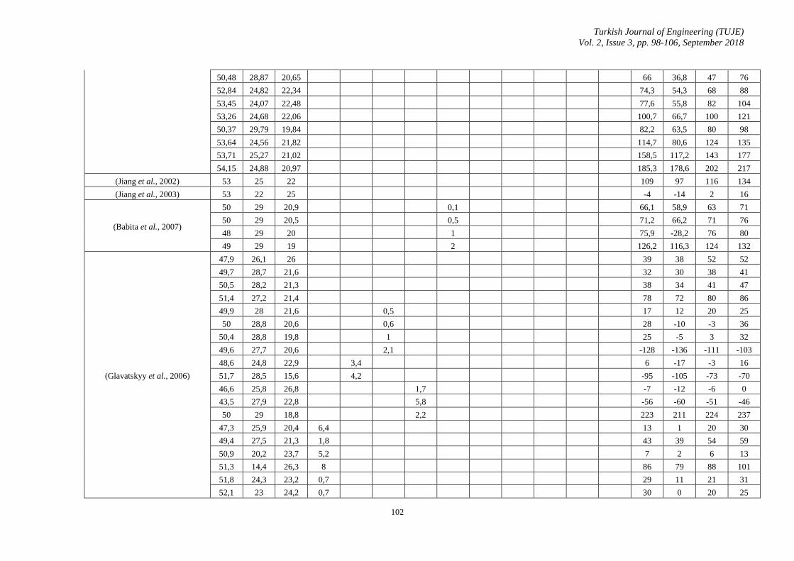
Turkish Journal of Engineering (TUJE)
Vol. 2, Issue 3, pp. 98-106, September 2018
102
50,48 28,87 20,65 66 36,8 47 76
52,84 24,82 22,34 74,3 54,3 68 88
53,45 24,07 22,48 77,6 55,8 82 104
53,26 24,68 22,06 100,7 66,7 100 121
50,37 29,79 19,84 82,2 63,5 80 98
53,64 24,56 21,82 114,7 80,6 124 135
53,71 25,27 21,02 158,5 117,2 143 177
54,15 24,88 20,97 185,3 178,6 202 217
(Jiang et al., 2002) 53 25 22 109 97 116 134
(Jiang et al., 2003) 53 22 25 -4 -14 2 16
(Babita et al., 2007)
50 29 20,9 0,1 66,1 58,9 63 71
50 29 20,5 0,5 71,2 66,2 71 76
48 29 20 1 75,9 -28,2 76 80
49 29 19 2 126,2 116,3 124 132
(Glavatskyy et al., 2006)
47,9 26,1 26 39 38 52 52
49,7 28,7 21,6 32 30 38 41
50,5 28,2 21,3 38 34 41 47
51,4 27,2 21,4 78 72 80 86
49,9 28 21,6 0,5 17 12 20 25
50 28,8 20,6 0,6 28 -10 -3 36
50,4 28,8 19,8 1 25 -5 3 32
49,6 27,7 20,6 2,1 -128 -136 -111 -103
48,6 24,8 22,9 3,4 6 -17 -3 16
51,7 28,5 15,6 4,2 -95 -105 -73 -70
46,6 25,8 26,8 1,7 -7 -12 -6 0
43,5 27,9 22,8 5,8 -56 -60 -51 -46
50 29 18,8 2,2 223 211 224 237
47,3 25,9 20,4 6,4 13 1 20 30
49,4 27,5 21,3 1,8 43 39 54 59
50,9 20,2 23,7 5,2 7 2 6 13
51,3 14,4 26,3 8 86 79 88 101
51,8 24,3 23,2 0,7 29 11 21 31
52,1 23 24,2 0,7 30 0 20 25
Turkish Journal of Engineering (TUJE)
Vol. 2, Issue 3, pp. 98-106, September 2018
103
(Koho et al., 2004)
51,7 24,4 22,7 1,2 53 34 41 62
47,3 30,3 20,3 2,1 53 32 42 61
48,9 29 19,5 2,6 65 52 53 76
48,8 29,2 20,1 1,9 45 27 49 64
48,6 27,5 21,6 2,3 31 22 33 41
48,9 26,2 22,6 2,3 57 45 58 70
49,4 27,9 20,3 54 42 54 59
50,2 27,4 21,1 61 50 63 77
49,6 28,3 20,7 53 36 48 64
50,1 28,2 20,9 0,8 44 28 40 64
49,2 29,6 21,2 31 28 35 38
52,2 27,3 20,6 132 112 102 122
(Lanska et al., 2004)
50,7 28,4 20,9 61 52 66 72
50,7 28,3 21 57 50 65 70
50,7 27,8 21,5 52 50 58 61
50,6 28,5 20,9 60 58 66 68
50 29,8 20,2 71 67 74 78
50 28,9 21,1 48 38 47 57
49,9 29,9 20,2 71 65 77 81
49,7 29,1 21,2 38 36 46 48
49,6 29,2 21,2 30 28 36 36
49,2 30,6 20,2 55 50 60 64
49,1 30,7 20,2 51 48 59 62
49 30,3 20,7 39 36 45 50
48,5 30,3 21,2 29 26 32 35
51 28,5 20,5 83 77 81 87
50,5 29,4 20,1 78 70 75 84
49,5 30,3 20,2 68 64 71 75
48,8 31,4 19,8 64 60 65 69
54,9 23,8 21,3 286 268 295 314
54 24,7 21,3 224 214 225 237
53,9 24,4 21,7 257 251 278 287
53,7 26,4 19,9 250 239 265 273

Turkish Journal of Engineering (TUJE)
Vol. 2, Issue 3, pp. 98-106, September 2018
104
53,3 24,6 22,1 192 186 195 203
52,9 25 22,1 75 71 81 90
52,8 25,7 21,5 117 94 104 131
52,7 26 21,3 161 143 151 173
52,4 25,6 22 150 141 151 161
52,3 27,4 20,3 125 118 130 135
51,7 27,7 20,6 110 96 108 121
51,5 26,8 21,7 120 101 107 127
51,2 27,4 21,4 98 93 98 102
51 28,7 20,3 106 93 103 112
50,5 30,4 19,1 118 103 110 124
47 33,1 19,9 53 50 56 58
(Santos et al., 2008) 50,55 36,33 13,12 -55 -66 -49 -41
(Wu et al., 2011) 37 50 10 3 -87 -120 -94 -61
(Turabi et al., 2016) 42,1 48,7 9,2 -6 -16 -6 4
(Kainuma et al., 1996)
50 50 674 660 707 719
50 46 4 589 567 593 608
50 42 8 473 459 485 503
50 38 12 341 285 304 368
50 34 16 191 128 134 192
50 30 20 -22 -34 -12 -4
44 46 10 268 259 348 362
45 40 15 116 81 94 119
55 30 15 386 378 433 449
(Zheng et al., 2011) 49 39 12 -13 -34 1 22
(Koyama et al., 2006) 50 36 14 -53 -63 -33 -23
(Aksoy et al., 2009)
50,3 35,9 13,8 3 -8 2 17
50,2 36,6 13,2 4 -3 7 18
51,5 36 12,5 73 65 76 85
50,3 39,6 10,1 171 95 107 184
51,9 42,7 5,4 436 348 359 468
(Caputo and Solomon 2017) 49,5 27,8 22,7 36,9 17,1 33,9 57,6
(Mostafaei et al., 2017) 49,6 30,8 19,6 36 31,5 42 46,5

Turkish Journal of Engineering (TUJE)
Vol. 2, Issue 3, pp. 98-106, September 2018
105
3. CONCLUSION
Shape memory alloys are defined undeniably
positioned in the technology. However, in terms of
production costs, it is necessary to search for alloy types
that will become an alternative to high-grade alloys such
as NiTi and to present the service of humanity. From this
point of view, successful studies with elements such as
manganese, which can be provided as cheaper than the
titanium element in nickel-based SHA, have been
investigated. It has been found that in the determined
thermal phase temperature transformations, the alloys'
high nickel, manganese and gallium ratios are largely
determinative. As a result of these studies, a wide range
of transformation temperatures have been identified and
found to be open to Research & Development. These
types of alloys that provide the wide range of conversion
can respond to many needs.
REFERENCES
Aksoy, S., M. Acet, E. F. Wassermann, T. Krenke, X.
Moya, L. Manosa, A. Planes and P. P. Deen (2009).
"Structural properties and magnetic interactions in
martensitic Ni-Mn-Sb alloys." Philosophical Magazine,
Vol. 89, No. 22-24, pp. 2093-2109.
Aldas, K., M. Eskil and İ. Özkul (2014). "Prediction of A
f temperature for copper based shape memory alloys."
Indian Journal of Engineering & Materials Science Vol.
21. pp. 429-437.
Aldas, K. and I. Ozkul (2016). "Determination of the
transformation temperatures of aged and low manganese
rated Cu-Al-Mn shape memory alloys." Journal of the
balkan tribological association, Vol. 22, No. 1, pp. 56-
65.
Babita, I., M. M. Raja, R. Gopalan, V. Chandrasekaran
and S. Ram (2007). "Phase transformation and magnetic
properties in Ni–Mn–Ga Heusler alloys." Journal of
alloys and compounds, Vol. 432, No. 1, pp. 23-29.
Buehler, W. J., J. Gilfrich and R. Wiley (1963). "Effect of
low‐temperature phase changes on the mechanical
properties of alloys near composition TiNi." Journal of
applied physics, Vol. 34, No. 5, pp. 1475-1477.
Canbay, C. A. (2017). "Kinetic parameters and structural
variations in Cu-Al-Mn and Cu-Al-Mn-Mg shape
memory alloys." AIP Conference Proceedings,
pp.120001.
Canbay, C. A., S. Ozgen and Z. K. Genc (2014). "Thermal
and microstructural investigation of Cu–Al–Mn–Mg
shape memory alloys." Applied Physics A, Vol. 117, No.
2, pp. 767-771.
Canbay, C. A. and İ. Özkul (2018). "Aging effects on
transformation temperatures and enthalpies for TiNi
alloy." Turkish Journal of Engineering (TUJE), Vol. 2,
No. 1, pp. 7-11.
Canbay, C. A., A. Tekataş and İ. Özkul (2017).
"Fabrication Of Cu-Al-Ni shape memory thin film by
thermal evopration." Turkish Journal of Engineering
(TUJE), Vol. 1, No. 2, pp. 27-32.
Caputo, M. and C. Solomon (2017). "A facile method for
producing porous parts with complex geometries from
ferromagnetic Ni-Mn-Ga shape memory alloys."
Materials Letters, Vol. 200, No., pp. 87-89.
Duerig, T. and A. Pelton (1994). "Ti-Ni shape memory
alloys." Materials properties handbook: titanium alloys,
Vol., No., pp. 1035-1048.
Eskil, M., K. Aldaş and İ. Özkul (2015). "Prediction of
thermodynamic equilibrium temperature of Cu-based
shape-memory smart materials." Metallurgical and
Materials Transactions A, Vol. 46, No. 1, pp. 134-142.
Glavatskyy, I., N. Glavatska, O. Söderberg, S.-P.
Hannula and J.-U. Hoffmann (2006). "Transformation
temperatures and magnetoplasticity of Ni–Mn–Ga
alloyed with Si, In, Co or Fe." Scripta materialia, Vol. 54,
No. 11, pp. 1891-1895.
Hodgson, D. E., W. Ming and R. J. Biermann (1990).
"Shape memory alloys." ASM International, Metals
Handbook, Tenth Edition., Vol. 2, No., pp. 897-902.
Huang, W. and W. Toh (2000). "Training two-way shape
memory alloy by reheat treatment." Journal of materials
science letters, Vol. 19, No. 17, pp. 1549-1550.
Jiang, C., G. Feng, S. Gong and H. Xu (2003). "Effect of
Ni excess on phase transformation temperatures of
NiMnGa alloys." Materials Science and Engineering: A,
Vol. 342, No. 1, pp. 231-235.
Jiang, C., G. Feng and H. Xu (2002). "Co-occurrence of
magnetic and structural transitions in the Heusler alloy Ni
53 Mn 25 Ga 22." Applied physics letters, Vol. 80, No. 9,
pp. 1619-1621.
Kainuma, R., K. Ishida and H. Nakano (1996).
"Martensitic transformations in NiMnAl β phase alloys."
Metallurgical and Materials Transactions A, Vol. 27, No.
12, pp. 4153-4162.
Koho, K., O. Söderberg, N. Lanska, Y. Ge, X. Liu, L.
Straka, J. Vimpari, O. Heczko and V. Lindroos (2004).
"Effect of the chemical composition to martensitic
transformation in Ni–Mn–Ga–Fe alloys." Materials
Science and Engineering: A, Vol. 378, No. 1, pp. 384-
388.
Koyama, K., K. Watanabe, T. Kanomata, R. Kainuma, K.
Oikawa and K. Ishida (2006). "Observation of field-
induced reverse transformation in ferromagnetic shape
memory alloy Ni 50 Mn 36 Sn 14." Applied physics
letters, Vol. 88, No. 13, pp. 132505.
Lanska, N., O. Söderberg, A. Sozinov, Y. Ge, K. Ullakko
and V. Lindroos (2004). "Composition and temperature
dependence of the crystal structure of Ni–Mn–Ga alloys."
Journal of Applied Physics, Vol. 95, No. 12, pp. 8074-
8078.

Turkish Journal of Engineering (TUJE)
Vol. 2, Issue 3, pp. 98-106, September 2018
106
Liu, Y. (2010). "Some factors affecting the
transformation hysteresis in shape memory alloys." Chen
HR, editor, Vol., No., pp. 361-369.
Ma, J., I. Karaman and R. D. Noebe (2010). "High
temperature shape memory alloys." International
Materials Reviews, Vol. 55, No. 5, pp. 257-315.
Mertmann, M. and G. Vergani (2008). "Design and
application of shape memory actuators." The European
Physical Journal Special Topics, Vol. 158, No. 1, pp.
221-230.
Mihálcz, I. (2001). "Fundamental characteristics and
design method for nickel-titanium shape memory alloy."
Periodica Polytechnica. Engineering. Mechanical
Engineering, Vol. 45, No. 1, pp. 75.
Mostafaei, A., K. A. Kimes, E. L. Stevens, J. Toman, Y.
L. Krimer, K. Ullakko and M. Chmielus (2017).
"Microstructural evolution and magnetic properties of
binder jet additive manufactured Ni-Mn-Ga magnetic
shape memory alloy foam." Acta Materialia, Vol. 131,
No., pp. 482-490.
Ozkul, I., C. A. Canbay, F. Aladağ and K. Aldaş (2017).
"The effect of the aging period on the martensitic
transformation and kinetic characteristic of at% Cu68.
09Al26. 1Ni1. 54Мn4. 27 shape memory alloy." Russian
Journal of Non-Ferrous Metals, Vol. 58, No. 2, pp. 130-
135.
Santos, J. D., T. Sanchez, P. Alvarez, M. Sanchez, J. L.
Sánchez Llamazares, B. Hernando, L. Escoda, J. J. Suñol
and R. Varga (2008). "Microstructure and magnetic
properties of Ni 50 Mn 37 Sn 13 Heusler alloy ribbons."
Journal of Applied Physics, Vol. 103, No. 7, pp. 07B326.
Schroeder, T. and C. Wayman (1977). "The two-way
shape memory effect and other “training” phenomena in
Cu Zn single crystals." Scripta metallurgica, Vol. 11, No.
3, pp. 225-230.
Sreekumar, M., T. Nagarajan and M. Singaperumal
(2009). "Application of trained NiTi SMA actuators in a
spatial compliant mechanism: Experimental
investigations." Materials & Design, Vol. 30, No. 8, pp.
3020-3029.
Stöckel, D. (1995). "The shape memory effect-
phenomenon, alloys and applications." California, Vol.
94539, No., pp. 1-13.
Sun, L., W. M. Huang, Z. Ding, Y. Zhao, C. C. Wang, H.
Purnawali and C. Tang (2012). "Stimulus-responsive
shape memory materials: a review." Materials & Design,
Vol. 33, No., pp. 577-640.
Turabi, A., P. Lázpita, M. Sasmaz, H. Karaca and V.
Chernenko (2016). "Magnetic and conventional shape
memory behavior of Mn–Ni–Sn and Mn–Ni–Sn (Fe)
alloys." Journal of Physics D: Applied Physics, Vol. 49,
No. 20, pp. 205002.
Wu, S. and S. Yang (2003). "Effect of composition on
transformation temperatures of Ni–Mn–Ga shape
memory alloys." Materials Letters, Vol. 57, No. 26, pp.
4291-4296.
Wu, Z., Z. Liu, H. Yang, Y. Liu and G. Wu (2011).
"Metamagnetic phase transformation in Mn 50 Ni 37 In
10 Co 3 polycrystalline alloy." Applied Physics Letters,
Vol. 98, No. 6, pp. 061904.
Zheng, H., D. Wu, S. Xue, J. Frenzel, G. Eggeler and Q.
Zhai (2011). "Martensitic transformation in rapidly
solidified Heusler Ni 49 Mn 39 Sn 12 ribbons." Acta
Materialia, Vol. 59, No. 14, pp. 5692-5699.
Copyright © Turkish Journal of Engineering (TUJE).
All rights reserved, including the making of copies
unless permission is obtained from the copyright
proprietors.

Turkish Journal of Engineering
107
Turkish Journal of Engineering (TUJE)
Vol. 2, Issue 3, pp. 107-112, September 2018
ISSN 2587-1366, Turkey
DOI: 10.31127/tuje.395259
Research Article
INVESTIGATION OF DISSOLUTION KINETICS OF Zn AND Mn FROM SPENT
ZINC-CARBON BATTERIES IN SULPHURIC ACID SOLUTION
Tevfik Agacayak *1 and Ali Aras 2
1 Selçuk University, Engineering Faculty, Department of Mining Engineering, Konya, Turkey
ORCID ID 0000–0001–8120–8804
2 Selçuk University, Engineering Faculty, Department of Mining Engineering, Konya, Turkey
ORCID ID 0000–0001–8111–6176
* Corresponding Author
Received: 15/02/2018 Accepted: 01/03/2018
ABSTRACT
The aim of this study is to examine the dissolution kinetics of zinc and manganese from spent zinc-carbon battery in
sulphuric acid solution. The leaching experiments were carried under the following conditions: leaching temperatures of
30°C, 40°C and 50°C; sulphuric acid concentration of 0.5 M; stirring speed of 400 rpm; solid/liquid ratio of 5/500 g/mL
and particle size of -53 µm. In these conditions, while all of the zinc was dissolved, about 69 % of manganese was dissolved.
To determine the kinetics of dissolution of the zinc and manganese in sulphuric acid medium, different shrinking core
models were applied to the dissolution recoveries obtained at variable temperatures. Kinetics analysis showed that the zinc
and manganese dissolution from spent zinc-carbon battery could be described by diffusion from product layer. The
activation energies (Ea) and Arrhenius constants for the dissolution reactions were calculated. Activation energies (Ea) were
determined for Zn and Mn as 94.53 kJ/mol and 1.41 kJ/mol, respectively.
Keywords: Leaching, Dissolution kinetics, Zn–C battery, Zn, Mn, Activation energy, Sulphuric acid
Turkish Journal of Engineering (TUJE)
Vol. 2, Issue 3, pp. 107-112, September 2018
108
1. INTRODUCTION
Zinc-carbon type dry cell batteries are being
commonly used during last 150 years in the world. There
are two types of zinc carbon batteries mainly as leclanche
battery and zinc chloride battery. A battery is an apparatus
which converts the chemical energy into electric energy
by an oxidation–reduction (redox) reaction. They are
widely used in small household apparatus like flash light,
toys, radios, watches, etc. In these batteries, anode
material is zinc and the cathode is a mixture of manganese
dioxide and carbon. Because of the spent zinc–carbon
batteries contain zinc, manganese dioxide and also zinc
oxide and manganese (III) oxide produced from
discharging reaction (Bernardes, et al., 2004; Park, et al.,
2006; Shin, et al., 2009), they are important secondary
source of Mn and Zn. During discharging, a chemical
change occurs in the battery which can be expressed by
the following reaction:
Zn+2MnO2 → ZnO + Mn2O3 (1)
A lot of studies were found related with
hydrometallurgical processes for recovery of manganese
and zinc from spent zinc–carbon batteries in the literature
(Shin, et al., 2009; Ferella, et al., 2008; Baba, et al., 2009;
sayilgan, et al., 2010; Gęga and Walkowiak, 2011;
Kursunoglu and Kaya, 2014; Buzatu, et al., 2014; Taner,
et al., 2016; Abedin, et al., 2017; Chen, et al., 2017).
Generally, these studies were carried out using only basic
solution, acidic solution (hydrochloric acid, sulphuric
acid) or reductive agents with these acid solutions.
However, dissolution kinetics of manganese and zinc
from spent zinc–carbon batteries were studied (Baba et
al., 2009; Gęga and Walkowiak, 2011; Taner, et al.,
2016).
Because, it is harmful to the environment discard of
spent batteries is prohibited by stringent environmental
regulations in most countries. In the event of the disposal
or incineration of waste batteries, heavy metals may
contaminate the environment. Therefore, it must be given
to importance to collecting and recycling of spent
batteries. Prevention of environmental pollution and
research for the recycling of precious metals have become
an important issue. For this reason, the application of
hydrometallurgical processes has been carried out
considering the economic and environmental suitability.
In this work, it is aimed to dissolution of manganese
and zinc in sulphuric acid solution from spent zinc carbon
batteries. In addition, the dissolution kinetics were
studied and the activation energies required for
dissolution were calculated.
2. MATERIAL AND METHOD
In this study, spent zinc–carbon batteries were used which
collected from Selçuk University spent battery boxes.
The plastic, paper and metal parts were removed from the
zinc-carbon batteries that were passed through processes
such as separation, dismantling. The separated pieces of
the spent zinc-carbon battery were weighed and the
weight percentages were determined as 56.42% black
paste, 13.84% steel can, 11.58% zinc can, 7.65% carbon
rod, 4.65% paper, 3.33% plastic and 2.53% metal cover
and bottom. The obtained black paste was dried at 105°C
for 24 hours. Moisture of black paste was calculated as
12.51%. The battery powder was ground using a ball mill
and sieved to obtain particle size less than 106 μm. The
original powder was washed to remove electrolyte with
distilled water in a glass vessel at 60°C and dried to
remove external impurities at 105°C for 24 hours. Then
the powder was burned for one hour at 600°C in the
furnace, to remove paper, plastic and carbon residues.
Sieving was carried out and -106+75, -75+53, -53 μm
particle size fractions were obtained. Approximately, 2
grams of sample was weighed and dissolved in the king
water (HNO3 + 3HCl) in a Teflon vessel. The solutions
were diluted with distilled water to 100 ml in a volumetric
flask. The amount of Mn and Zn was measured using a
GBC brand SensAA model flame atomic absorption
spectrometer (AAS). The manganese-zinc contents of
waste battery powder of the original (-106 μm), washed
(-106 μm) and -53 μm particle size were given in Table 1.
Table 1. Zn–Mn content of spent zinc–carbon battery
Particle size, μm Zn,% Mn,%
Original (-106) 21.52 34.34
Washed (-106) 22.87 35.87
-53 20.11 36.46
The washed powders were analyzed by X-ray diffraction
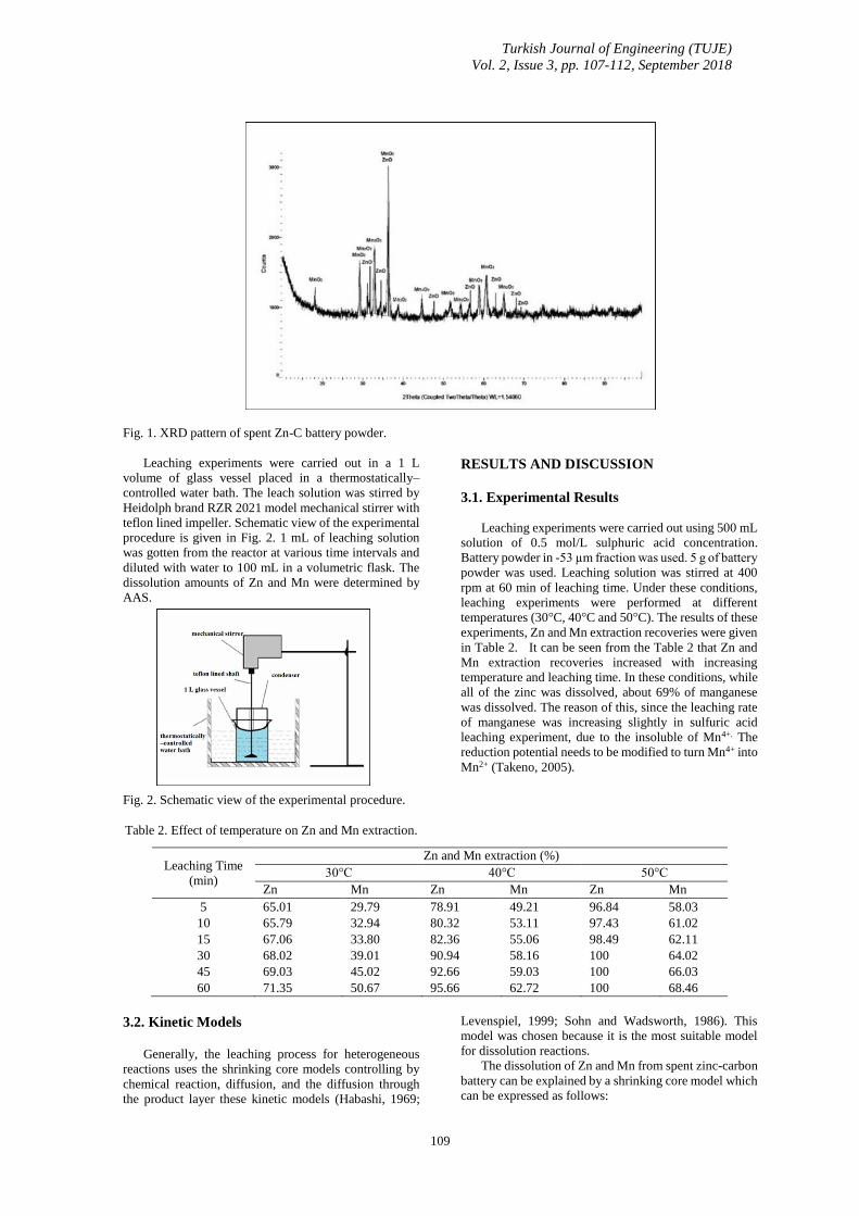
(XRD) to determine the mineralogical composition of
powders and shown in Fig. 1. XRD analyses showed the
presence of ZnO, MnO2 and Mn2O3.
Turkish Journal of Engineering (TUJE)
Vol. 2, Issue 3, pp. 107-112, September 2018
109
Fig. 1. XRD pattern of spent Zn-C battery powder.
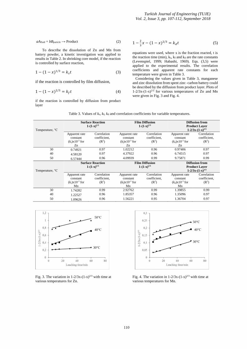
Leaching experiments were carried out in a 1 L
volume of glass vessel placed in a thermostatically–
controlled water bath. The leach solution was stirred by
Heidolph brand RZR 2021 model mechanical stirrer with
teflon lined impeller. Schematic view of the experimental
procedure is given in Fig. 2. 1 mL of leaching solution
was gotten from the reactor at various time intervals and
diluted with water to 100 mL in a volumetric flask. The
dissolution amounts of Zn and Mn were determined by
AAS.
Fig. 2. Schematic view of the experimental procedure.
RESULTS AND DISCUSSION
3.1. Experimental Results
Leaching experiments were carried out using 500 mL
solution of 0.5 mol/L sulphuric acid concentration.
Battery powder in -53 µm fraction was used. 5 g of battery
powder was used. Leaching solution was stirred at 400
rpm at 60 min of leaching time. Under these conditions,
leaching experiments were performed at different
temperatures (30°C, 40°C and 50°C). The results of these
experiments, Zn and Mn extraction recoveries were given
in Table 2. It can be seen from the Table 2 that Zn and
Mn extraction recoveries increased with increasing
temperature and leaching time. In these conditions, while
all of the zinc was dissolved, about 69% of manganese
was dissolved. The reason of this, since the leaching rate
of manganese was increasing slightly in sulfuric acid
leaching experiment, due to the insoluble of Mn4+. The
reduction potential needs to be modified to turn Mn4+ into
Mn2+ (Takeno, 2005).
Table 2. Effect of temperature on Zn and Mn extraction.
3.2. Kinetic Models
Generally, the leaching process for heterogeneous
reactions uses the shrinking core models controlling by
chemical reaction, diffusion, and the diffusion through
the product layer these kinetic models (Habashi, 1969;
Levenspiel, 1999; Sohn and Wadsworth, 1986). This
model was chosen because it is the most suitable model
for dissolution reactions.
The dissolution of Zn and Mn from spent zinc-carbon
battery can be explained by a shrinking core model which
can be expressed as follows:
Leaching Time
(min)
Zn and Mn extraction (%)
30°C 40°C 50°C
Zn Mn Zn Mn Zn Mn
5 65.01 29.79 78.91 49.21 96.84 58.03
10 65.79 32.94 80.32 53.11 97.43 61.02
15 67.06 33.80 82.36 55.06 98.49 62.11
30 68.02 39.01 90.94 58.16 100 64.02
45 69.03 45.02 92.66 59.03 100 66.03
60 71.35 50.67 95.66 62.72 100 68.46
Turkish Journal of Engineering (TUJE)
Vol. 2, Issue 3, pp. 107-112, September 2018
110
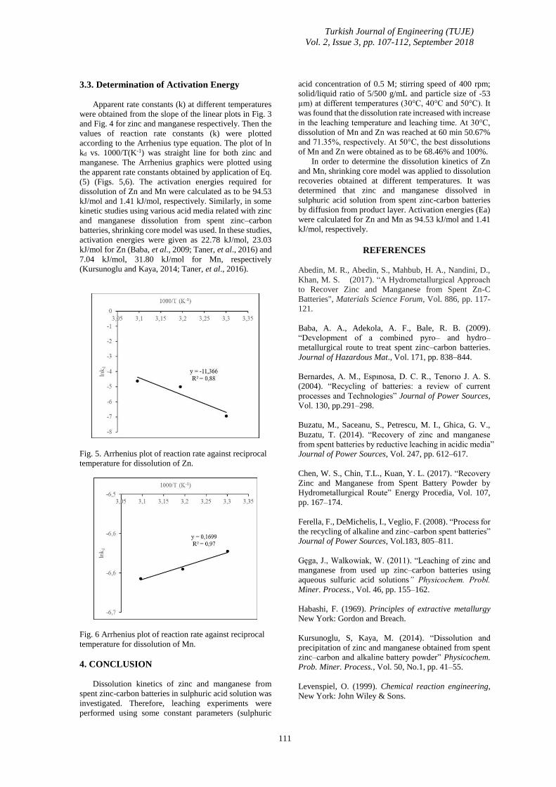
aAfluid + bBparticle → Product (2)
To describe the dissolution of Zn and Mn from
battery powder, a kinetic investigation was applied to
results in Table 2. In shrinking core model, if the reaction
is controlled by surface reaction,
1 − (1 − 𝑥)1/3 = 𝑘𝑠𝑡 (3)
if the reaction is controlled by film diffusion,
1 − (1 − 𝑥)2/3 = 𝑘𝑓𝑡 (4)
if the reaction is controlled by diffusion from product
layer
1 −2
3𝑥 − (1 − 𝑥)2/3 = 𝑘𝑑𝑡 (5)
equations were used, where x is the fraction reacted, t is
the reaction time (min), ks, kf and kd are the rate constants
(Levenspiel, 1999; Habashi, 1969). Eqs. (3,5) were
applied to the experimental results. The correlation
coefficients and apparent rate constants for each
temperature were given in Table 3.
Considering the values given in Table 3, manganese
and zinc dissolution from spent zinc–carbon battery could
be described by the diffusion from product layer. Plots of
1-2/3x-(1-x)2/3 for various temperatures of Zn and Mn
were given in Fig. 3 and Fig. 4.
Table 3. Values of ks, kf, kd and correlation coefficients for variable temperatures.
Temperature, °C
Surface Reaction
1-(1-x)1/3
Film Diffusion
1-(1-x)2/3
Diffusion from
Product Layer
1-2/3x-(1-x)2/3
Apparent rate constant
(ks)x10-3 for
Zn
Correlation coefficient,
(R2)
Apparent rate constant
(kf)x10-3 for
Zn
Correlation coefficient,
(R2)
Apparent rate constant
(kd)x10-3 for
Zn
Correlation coefficient,
(R2)
30 0.74921 0.97 1.02212 0.96 0.97406 0.97
40 4.58120 0.97 4.37922 0.96 6.74515 0.97
50 6.57444 0.96 4.09939 0.99 9.75871 0.99
Temperature, °C
Surface Reaction
1-(1-x)1/3
Film Diffusion
1-(1-x)2/3
Diffusion from
Product Layer
1-2/3x-(1-x)2/3
Apparent rate
constant
(ks)x10-3 for Mn
Correlation
coefficient,
(R2)
Apparent rate
constant
(kf)x10-3 for Mn
Correlation
coefficient,
(R2)
Apparent rate
constant
(kd)x10-3 for Mn
Correlation
coefficient,
(R2)
30 1.74282 0.99 2.92762 0.99 1.39855 0.99
40 1.22527 0.96 1.85357 0.96 1.35096 0.97
50 1.09626 0.96 1.56221 0.95 1.36704 0.97
Fig. 3. The variation in 1-2/3x-(1-x)2/3 with time at
various temperatures for Zn.
Fig. 4. The variation in 1-2/3x-(1-x)2/3 with time at
various temperatures for Mn.
30°C
40°C
50°C
40°C
50°C
30°C
Turkish Journal of Engineering (TUJE)
Vol. 2, Issue 3, pp. 107-112, September 2018
111
3.3. Determination of Activation Energy
Apparent rate constants (k) at different temperatures
were obtained from the slope of the linear plots in Fig. 3
and Fig. 4 for zinc and manganese respectively. Then the
values of reaction rate constants (k) were plotted
according to the Arrhenius type equation. The plot of ln
kd vs. 1000/T(K-1) was straight line for both zinc and
manganese. The Arrhenius graphics were plotted using
the apparent rate constants obtained by application of Eq.
(5) (Figs. 5,6). The activation energies required for
dissolution of Zn and Mn were calculated as to be 94.53
kJ/mol and 1.41 kJ/mol, respectively. Similarly, in some
kinetic studies using various acid media related with zinc
and manganese dissolution from spent zinc–carbon
batteries, shrinking core model was used. In these studies,
activation energies were given as 22.78 kJ/mol, 23.03
kJ/mol for Zn (Baba, et al., 2009; Taner, et al., 2016) and
7.04 kJ/mol, 31.80 kJ/mol for Mn, respectively
(Kursunoglu and Kaya, 2014; Taner, et al., 2016).
Fig. 5. Arrhenius plot of reaction rate against reciprocal
temperature for dissolution of Zn.
Fig. 6 Arrhenius plot of reaction rate against reciprocal
temperature for dissolution of Mn.
4. CONCLUSION
Dissolution kinetics of zinc and manganese from
spent zinc-carbon batteries in sulphuric acid solution was
investigated. Therefore, leaching experiments were
performed using some constant parameters (sulphuric
acid concentration of 0.5 M; stirring speed of 400 rpm;
solid/liquid ratio of 5/500 g/mL and particle size of -53
µm) at different temperatures (30°C, 40°C and 50°C). It
was found that the dissolution rate increased with increase
in the leaching temperature and leaching time. At 30°C,
dissolution of Mn and Zn was reached at 60 min 50.67%
and 71.35%, respectively. At 50°C, the best dissolutions
of Mn and Zn were obtained as to be 68.46% and 100%.
In order to determine the dissolution kinetics of Zn
and Mn, shrinking core model was applied to dissolution
recoveries obtained at different temperatures. It was
determined that zinc and manganese dissolved in
sulphuric acid solution from spent zinc-carbon batteries
by diffusion from product layer. Activation energies (Ea)
were calculated for Zn and Mn as 94.53 kJ/mol and 1.41
kJ/mol, respectively.
REFERENCES
Abedin, M. R., Abedin, S., Mahbub, H. A., Nandini, D.,
Khan, M. S. (2017). “A Hydrometallurgical Approach
to Recover Zinc and Manganese from Spent Zn-C
Batteries", Materials Science Forum, Vol. 886, pp. 117-
121.
Baba, A. A., Adekola, A. F., Bale, R. B. (2009).
“Development of a combined pyro– and hydro–
metallurgical route to treat spent zinc–carbon batteries.
Journal of Hazardous Mat., Vol. 171, pp. 838–844.
Bernardes, A. M., Espınosa, D. C. R., Tenorıo J. A. S.
(2004). “Recycling of batteries: a review of current
processes and Technologies” Journal of Power Sources,
Vol. 130, pp.291–298.
Buzatu, M., Saceanu, S., Petrescu, M. I., Ghica, G. V.,
Buzatu, T. (2014). “Recovery of zinc and manganese
from spent batteries by reductive leaching in acidic media”
Journal of Power Sources, Vol. 247, pp. 612–617.
Chen, W. S., Chin, T.L., Kuan, Y. L. (2017). “Recovery
Zinc and Manganese from Spent Battery Powder by
Hydrometallurgical Route” Energy Procedia, Vol. 107,
pp. 167–174.
Ferella, F., DeMichelis, I., Veglio, F. (2008). “Process for
the recycling of alkaline and zinc–carbon spent batteries”
Journal of Power Sources, Vol.183, 805–811.
Gęga, J., Walkowiak, W. (2011). “Leaching of zinc and
manganese from used up zinc–carbon batteries using
aqueous sulfuric acid solutions” Physicochem. Probl.
Miner. Process., Vol. 46, pp. 155–162.
Habashi, F. (1969). Principles of extractive metallurgy
New York: Gordon and Breach.
Kursunoglu, S, Kaya, M. (2014). “Dissolution and
precipitation of zinc and manganese obtained from spent
zinc–carbon and alkaline battery powder” Physicochem.
Prob. Miner. Process., Vol. 50, No.1, pp. 41–55.
Levenspiel, O. (1999). Chemical reaction engineering,
New York: John Wiley & Sons.

Turkish Journal of Engineering (TUJE)
Vol. 2, Issue 3, pp. 107-112, September 2018
112
Park, J., Kang, J., Sohn, J., Yang, D., Shin, S. (2006).
“Physical treatment for recycling commercialization of
spent household batteries” J. Korean Inst. Resour.
Recycl., Vol:15 No:6, pp. 48–55.
Sayilgan, E., Kukrer, T., Yigit, N. O., Civelekoglu, G.,
Kitis, M. (2010). “Acidic leaching and precipitation of
zinc and manganese from spent battery powders using
various reductants” J. Hazard. Mater., Vol. 173, pp.137–
143.
Shin, S., Senanayake, G., Sohn J., Park, J., Kang, J., Yang
D., Kim T. (2009). “Separation of zinc from spent zinc–
carbon batteries by selective leaching with sodium
hydroxide”, Hydrometallurgy, Vol. 96, pp. 349–353.
Sohn, H. Y., Wadsworth, M. E. (1986). Cr'nética de los
procesos de la Metalurgia Extractiva (translated from
English Version). Ed. Trillas, Mexico. Takeno, N., (2005)
“Atlas of Eh-pH diagrams Intercomparison of
thermodynamic databases”, National Institute of
Advanced Industrial Science and Technology, Japan.
Taner, H. A., Aras, A., Agacayak, T. (2016).
“Determination of dissolution kinetics of manganese and
zinc from spent zinc–carbon batteries in acidic media” 1.
International Academic Research Congress, Ines 2016,
Anyalya/Side/ Turkey, pp. 379-383.
Copyright © Turkish Journal of Engineering (TUJE).
All rights reserved, including the making of copies
unless permission is obtained from the copyright
proprietors.

Turkish Journal of Engineering
113
Turkish Journal of Engineering (TUJE)
Vol. 2, Issue 3, pp. 113-118, September 2018
ISSN 2587-1366, Turkey
DOI: 10.31127/tuje.385008
Research Article
COMPARATIVE STUDY OF REGIONAL CRASH DATA IN TURKEY
Murat Ozen *1
Mersin University, Engineering Faculty, Department of Civil Engineering, Mersin, Turkey
ORCID ID 0000-0002-1745-7483
* Corresponding Author
Received: 28/01/2018 Accepted: 10/04/2018
ABSTRACT
This study provides a comparative analysis of traffic safety in Turkey across the seven geographic regions over a 11 year
time frame (2006 to 2016). The comparisons are performed in relative terms and absolute terms. Fatal and/or injury (FI)
crashes per million population and per million registered vehicles were used to quantify safety. For the ordinal analysis,
rates for the regions were ranked individually for each year as well as for the 11 years aggregated. An examination of the
results indicated that the relative ranks of the regions were stable over the study period. Depending on the safety measure
used, the relative rankings of regions varied. It means that a region ranked at the top (high crash rate) for one safety measure
does not need to be ranked again at the top for other safety measure. For the cardinal analysis, the computed rates were
used. These results were consistent with those from the ordinal analysis, but showed greater variability in the rates over
time, which means that FI crash rates significantly increased over the time. A Geographic Information Systems based
thematic maps were used to support these efforts.
Keywords: Comparative Safety Analysis, Crash Rates, Data Visualization, Traffic Safety
Turkish Journal of Engineering (TUJE)
Vol. 2, Issue 3, pp. 113-118, September 2018
114
1. INTRODUCTION
Even though there has been significant public policy
attention and improvements in traffic safety policies and
practices in Turkey, 61 people died per billion vehicle-km
in traffic crashes in 2016 (TGDH, 2017; TurkStat,
2018a). In spite of significant improvements in national
highway network, there has been an increase in fatal
and/or injury (FI) crashes over the last decade (TurkStat,
2018a). The distribution of crashes across the nation is
also of importance to transportation system owners.
National and local safety programs aim to reduce crashes
and the severity of their outcomes within their
jurisdictions. Development of geographically appropriate
safety strategies requires estimating pertinent crash and
exposure data at the relevant spatial scale. While data
required to identify safety risks are collected at the local
level, published databases are typically available only at
larger scales. Thus, there is a need to deduce data at the
local level (i.e., lower levels of spatial aggregation) from
partially complete or surrogate datasets that are available
at a higher level of aggregation.
FI crashes are reported by the traffic police and
gendarmerie units according to their areas of
responsibility in Turkey. Disaggregate statistics of these
crashes are published annually by Turkish Statistical
Institute (TurkStat). This aggregate database provides
temporal and provincial distribution of the crashes as well
as type of vehicles involved, classification of the crash
locations as well as gender and age distribution of the
crash victims. Due to the lack of disaggregate crash level
data at the national level, province and regional variations
of traffic safety have not been examined in detail.
Recently, Atalay and Tortum (2015) compared the
number of fatalities per traffic crashes and per kilometer
of road network across the 81 provinces of Turkey. The
results showed that number of fatalities per crash are
higher in less developed provinces, whereas number of
fatalities per length of road network are higher in
developed provinces. In other study, Erdogan (2009)
studied the provincial level differences in number of FI
crashes and number of fatalities. Population and number
of registered vehicles were used to quantify safety and
results indicated that provinces with higher FI crashes and
fatalities were located in the provinces that contain the
roads connecting the İstanbul, Ankara, and Antalya
provinces. However, there is no study focusing on traffic
safety at the regional level in Turkey.
This study provides a comparative analysis of the FI
crashes across the seven geographic regions in Turkey
from 2006 to 2016 (additional information is provided in
Appendix A). The comparisons are performed in relative
terms and absolute terms. Since vehicle-km data are not
available either province or regional level, number of FI
crashes per million population and per million registered
vehicles are used to quantify safety. The principal sources
of data used in this study is TurkStat.
2. METHODOLOGY
Number of FI crashes per million population and per
million registered vehicles were determined for each
geographic region annually for the study period. A
Geographic Information Systems based thematic maps
were used to support these efforts.
Traditional statistical tests based on the normality
assumption of the data. Since FI crash rates do not follow
normal distribution either across the regions or over the
years, nonparametric methods need to be used to study FI
crash rates. An appropriate test to use for this purpose is
the Kruskal-Wallis nonparametric test. In this study,
hypotheses of the Kruskall-Wallis H test was that:
HO: FI crash rates are the same for each region from 2006
to 2016
H1: FI crash rates are not the same for each region from
2006 to 2016.
Based on the Kruskall-Wallis test, the null hypothesis,
Ho, is to be rejected at the (100-α) percent level of
confidence if the test statistic, H, falls in the critical region
H > χα2 with v = (k-1) degrees of freedom. To control the
familywise type I error in Kruskall-Wallis H test; the
probability of rejecting at least one pair hypothesis given
all pairwise hypotheses are true, adjusted p-values are
calculated and used to make the decision for each pair.
The following equations was used to calculate adjusted p-
values for each of pairwise hypothesis. If the adjusted p-
value is bigger than 1, it is set to 1.
𝑝𝑎𝑑𝑗 = 𝑝𝐾(𝐾 − 1)/2 (1)
where; K = number of pairwise hypothesis, and p =
significance level of pairwise hypothesis.
3. RESULTS
FI crash rates were calculated annually for each
geographic region based on per million population and
per million registered vehicles. The results are presented
thematically in Tables B1 to B2 (see Appendix). It is
noted that the numbers of the regions are given randomly.
In these tables, a graded color pattern is used to indicate
FI crash rates. The color gradation ranges from red to
yellow or green. Dark red is used to indicate the higher FI
crash rates and worse safety records, and dark green is
used to indicate lower FI crash rates and best safety
records. Lighter red, yellow and lighter green colors are
used to achieve gradation.
Table B1 presents FI crash rates of each region per
million population for each year during the study period.
Table B2 presents FI crash rates of each region per
million registered vehicles for each year during the study
period. In addition, the average FI crash rates for each
measure for the entire 11 year period as a whole are given
in these tables. It is seen that FI crash rates for regions
significantly increased for each measure from 2006 to
2016. Furthermore, Table B1 and B2 clearly indicate the
stability of the relative FI crash rates of regions across the
years. They show that regions that tended to have lower
FI crash rates, had lower crash rates across the years; and,
regions that tended to have higher FI crash rates, had
higher crash rates across the years.
Kruskall-Wallis pairwise comparisons implied that FI
crash rates per million population are not the same across
the regions from 2006 to 2016 (i.e. H = 31.50 >
χ0.05,92 =12.59). Fig. 1 and 2 present box plot and 95%
confidence interval of FI crash rates of regions per million
population. It is seen that FI crash rates in Central
Anatolia Region (Region 5), Mediterranean Region
(Region 4) and Aegean Region (Region 2) seems
Turkish Journal of Engineering (TUJE)
Vol. 2, Issue 3, pp. 113-118, September 2018
115
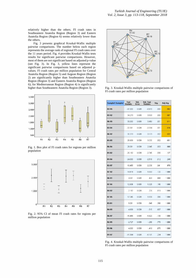
relatively higher than the others. FI crash rates in
Southeastern Anatolia Region (Region 3) and Eastern
Anatolia Region (Region 6) seems relatively lower than
the others.
Fig. 3 presents graphical Kruskal-Wallis multiple
pairwise comparisons. The number below each region
represents the average rank of regional FI crash rates over
the 11 years period. Fig. 4 provides Kruskal-Wallis tests
results for significant pairwise comparisons. However,
most of them are not significant based on adjusted p-value
(see Fig. 3). In Fig. 3, yellow lines represent the
significant pairwise comparisons based on adjusted p-
values. FI crash rates per million population for Central
Anatolia Region (Region 5) and Aegean Region (Region
2) are significantly higher than Southeastern Anatolia
Region (Region 3) and Eastern Anatolia Region (Region
6); for Mediterranean Region (Region 4) is significantly
higher than Southeastern Anatolia Region (Region 3).
Fig. 1. Box plot of FI crash rates for regions per million
population
Fig. 2. 95% CI of mean FI crash rates for regions per
million population
Fig. 3. Kruskal-Wallis multiple pairwise comparisons of
FI crash rates per million population
Fig. 4. Kruskal-Wallis multiple pairwise comparisons of
FI crash rates per million population
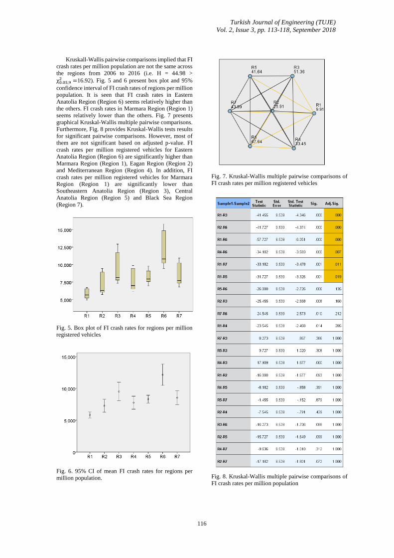
Turkish Journal of Engineering (TUJE)
Vol. 2, Issue 3, pp. 113-118, September 2018
116
Kruskall-Wallis pairwise comparisons implied that FI
crash rates per million population are not the same across
the regions from 2006 to 2016 (i.e. H = 44.98 >
χ0.05,92 =16.92). Fig. 5 and 6 present box plot and 95%
confidence interval of FI crash rates of regions per million
population. It is seen that FI crash rates in Eastern
Anatolia Region (Region 6) seems relatively higher than
the others. FI crash rates in Marmara Region (Region 1)
seems relatively lower than the others. Fig. 7 presents
graphical Kruskal-Wallis multiple pairwise comparisons.
Furthermore, Fig. 8 provides Kruskal-Wallis tests results
for significant pairwise comparisons. However, most of
them are not significant based on adjusted p-value. FI
crash rates per million registered vehicles for Eastern
Anatolia Region (Region 6) are significantly higher than
Marmara Region (Region 1), Eagan Region (Region 2)
and Mediterranean Region (Region 4). In addition, FI
crash rates per million registered vehicles for Marmara
Region (Region 1) are significantly lower than
Southeastern Anatolia Region (Region 3), Central
Anatolia Region (Region 5) and Black Sea Region
(Region 7).
Fig. 5. Box plot of FI crash rates for regions per million
registered vehicles
Fig. 6. 95% CI of mean FI crash rates for regions per
million population.
Fig. 7. Kruskal-Wallis multiple pairwise comparisons of
FI crash rates per million registered vehicles
Fig. 8. Kruskal-Wallis multiple pairwise comparisons of
FI crash rates per million population

Turkish Journal of Engineering (TUJE)
Vol. 2, Issue 3, pp. 113-118, September 2018
117
Fig. 9 and 10 provide thematic maps based on the
average ranks of the provinces for each of the safety
measures used in this study. In these maps, the red colored
provinces have the highest rates while the green colored
provinces have the lowest rates. An examination for Fig.
1 to 2 reveal some interesting patterns in the spatial
distribution of the relative safety ranks of the regions.
Overall, it can be seen that Marmara Region (Region 1)
tend to have best safety records. Relative safety records
of Aegean Region (Region 2), Eastern Anatolia Region
(Region 6) and Southeastern Anatolia Region (Region 3)
are significantly different for million population and
million registered vehicles measures. For instance,
Eastern Anatolia Region (Region 6) has the best safety
records for FI crash rates per million population, however,
it has the worst safety records for FI crash rates per
million registered vehicles.
Fig 9. Average FI crash rates per million population for
regions from 2006 to 2016
Fig. 10. Average FI crash rates per million registered
vehicle for regions from 2006 to 2016
4. CONCLUSION
This paper summarized efforts of and findings from a
study to examine regional level FI crash trends and
perform comparative analyses of safety records 2006 to
2016. The comparisons were performed in relative terms
(ordinal scale or based on rates) and absolute terms
(cardinal or rank ordered scale). Two safety measures
were used to evaluate safety: million population and
million registered vehicles. Data were obtained from
publications maintained by TurkStat.
An examination of the results indicated that the
relative ranks of the regions were stable over the study
period for each safety measure. Non-parametric statistical
tests and thematic maps used to support comparative
analyses. Specifically, the Kruskal-Wallis nonparametric
test was used in this study. The results showed that the FI
crash rates are not the same across the regions.
Furthermore, the analyses also revealed that depending on
the safety measure used, the relative rankings of regions
varied (i.e., a region ranked at the top (high crash rate) for
one safety measure does not need to be ranked again at
the top for other safety measure). This figure is resulted
from significantly different vehicle ownership rate across
the regions in Turkey. For the cardinal analysis the
computed rates were used. These results were consistent
with those from the ordinal analysis, but it was showed
that FI crash rates significantly increased over the time.
For broad macro level analyses a more representative
vehicle-km measure is required to study relative safety
records of regions. However, it is available only for
national level in Turkey. Furthermore, if specific analyses
are required, then safety measures should be defined
based on the desired evaluations. For example, if the goal
were to address rural safety, the measures should be
computed using rural fatal and/or injury crashes, rural
vehicle-km, and the extent of rural kilometers of road
network. This paper explored methods to analyze regional
differences in road traffic safety. The results document
the validity and promise of the methods. These methods
could be expanded for policy and operational analyses.
REFERENCES
Erdogan, S. (2009). “Explorative spatial analysis of
traffic accident statistics and road mortality among the
provinces of Turkey”. Journal of safety research, Vol. 40,
No. 5, 341-351.
OECD/ITF. (2016). Organisation for Economic Co-
operation and Development/International Transport
Forum. Road Safety Annual Report 2016, Paris. OECD
Publishing, 2016.
TGDH, Turkish General Directorate of Highways.
(2017). Karayolları Üzerindeki Seyir ve Taşımalar.
Turkey.
http://www.kgm.gov.tr/SiteCollectionDocuments/KGM
documents/Istatistikler/SeyirveTasimalar/SeyirVeTasim
alar.pdf [Accessed 10 Dec 2017].
Tortum, A. and Atalay, A. (2015). “Spatial analysis of
road mortality rates in Turkey.” In Proceedings of the
Institution of Civil Engineers-Transport, Vol. 168, No. 6,
pp. 532-542.
TurkStat, Turkish Statistical Institute. (2018a). Road
Traffic Accident Statistics, 2015.
http://www.turkstat.gov.tr/PreHaberBultenleri.do?id=21
611 [Accessed 10 Dec 2017].
TurkStat, Turkish Statistical Institute. (2018b). Road
Traffic Accident Statistics, 2016.
http://www.turkstat.gov.tr/PreHaberBultenleri.do?id=24
606 [Accessed 10 Dec 2017].
Copyright © Turkish Journal of Engineering (TUJE).
All rights reserved, including the making of copies
unless permission is obtained from the copyright
proprietors.
Turkish Journal of Engineering (TUJE)
Vol. 2, Issue 3, pp. 113-118, September 2018
118
Appendix A: Geographic Regions in Turkey It is noted that the numbers of the regions are given randomly.
Marmara Region (Region 1): Balıkesir, Bilecik, Bursa, Çanakkale, Edirne, İstanbul, Kırklareli, Kocaeli, Sakarya,
Tekirdağ, Yalova.
Aegean Region (Region 2): Afyon, Aydın, Denizli, İzmir, Kütahya, Manisa, Muğla, Uşak.
Southeastern Anatolia Region (Region 3): Adıyaman, Batman, Diyarbakır, Gaziantep, Kilis, Mardin, Siirt, Urfa, Şırnak.
Mediterranean Region (Region 4): Adana, Antalya, Burdur, Hatay, Isparta, Kahramanmaraş, Mersin, Osmaniye.
Central Anatolia Region (Region 5): Aksaray, Ankara, Çankırı, Eskişehir, Karaman, Kayseri, Kırıkkale, Kırşehir, Konya,
Nevşehir, Niğde, Sivas, Yozgat.
Eastern Anatolia Region (Region 6): Ağrı, Ardahan, Bingöl, Bitlis, Elazığ, Erzincan, Erzurum, Hakkari, Iğdır, Kars,
Malatya, Muş, Tunceli, Van.
Black Sea Region (Region 7): Amasya, Artvin, Bartın, Bayburt, Bolu, Çorum, Düzce, Giresun, Gümüşhane, Karabük,
Kastamonu, Ordu, Rize, Samsun, Sinop, Tokat, Trabzon, Zonguldak
Fig. A1. Geographical regions in Turkey
Appendix B: FI Crash Rates Table B1. FI crash rates for regions per million population
Region 2006 2007 2008 2009 2010 2011 2012 2013 2014 2015 2016 Average
2006-2016
Marmara (R1) 930 1061 1051 1087 1091 1233 1376 1557 1621 1707 1718 1312
Aegean (R2) 1479 1564 1489 1544 1597 1826 2197 2766 2961 3183 3150 2160
Southeastern
Anatolia (R3) 707 717 706 794 834 936 1153 1538 1564 1718 1524 1108
Mediterranean (R4) 1388 1481 1432 1522 1608 1848 2164 2749 2796 3061 3020 2097
Central
Anatolia (R5) 1565 1678 1558 1720 1803 2000 2371 2675 2621 2745 2786 2138
Eastern
Anatolia (R6) 699 749 726 808 942 1017 1159 1558 1688 1815 1797 1178
Black
Sea (R7) 1065 1181 1093 1207 1304 1433 1608 2192 2304 2529 2702 1692
Table B2. FI crash rates for regions per million registered vehicle
Region 2006 2007 2008 2009 2010 2011 2012 2013 2014 2015 2016 Average
2006-2016
Marmara (R1) 4927 5378 5141 5265 5191 5669 6098 6666 6715 6731 6456 5840
Aegean (R2) 6276 6278 5725 5846 5852 6305 7263 8859 9175 9428 8979 7271
Southeastern
Anatolia (R3) 8163 7839 7329 7771 7616 8077 9414 12098 12058 12916 11335 9511
Mediterranean (R4) 6626 6673 6130 6346 6469 6997 7802 9571 9403 9867 9459 7758
Central
Anatolia (R5) 7636 7826 6986 7502 7551 7943 8989 9754 9214 9202 8963 8324
Eastern
Anatolia (R6) 10189 10294 9449 9871 10621 10811 11614 14783 15399 15784 14859 12152
Black Sea (R7)
7384 7710 6788 7189 7313 7483 7935 10243 10255 10651 10920 8534

Turkish Journal of Engineering
119
Turkish Journal of Engineering (TUJE)
Vol. 2, Issue 3, pp. 119-124, September 2018
ISSN 2587-1366, Turkey
DOI: 10.31127/tuje.408976
Research Article
PERFORMANCE COMPARISON OF ANFIS, ANN, SVR, CART AND MLR
TECHNIQUES FOR GEOMETRY OPTIMIZATION OF CARBON NANOTUBES
USING CASTEP
Mehmet Acı 1, Çiğdem İnan Acı *2 and Mutlu Avcı 3
1 Mersin University, Faculty of Engineering, Department of Computer Engineering, Mersin, Turkey
ORCID ID 0000-0002-7245-8673
2 Mersin University, Faculty of Engineering, Department of Computer Engineering, Mersin, Turkey
ORCID ID 0000-0002-0028-9890
3 Çukurova University, Faculty of Engineering, Department of Biomedical Engineering, Adana, Turkey
ORCID ID 0000-0002-4412-4764
* Corresponding Author
Received: 22/03/2018 Accepted: 10/04/2018
ABSTRACT
Density Functional Theory (DFT) calculations used in the Carbon Nanotubes (CNT) design take a very long time even in
the simulation environment as it is well known in literature. In this study, calculation time of DFT for geometry optimization
of CNT is reduced from days to minutes using seven artificial intelligence-based and one statistical-based methods and the
results are compared. The best results are achieved from ANFIS and ANN based models and these models can be used
instead of CNT simulation software with high accuracy.
Keywords: Geometry Optimization, Cnt, Dft, Artificial Intelligence
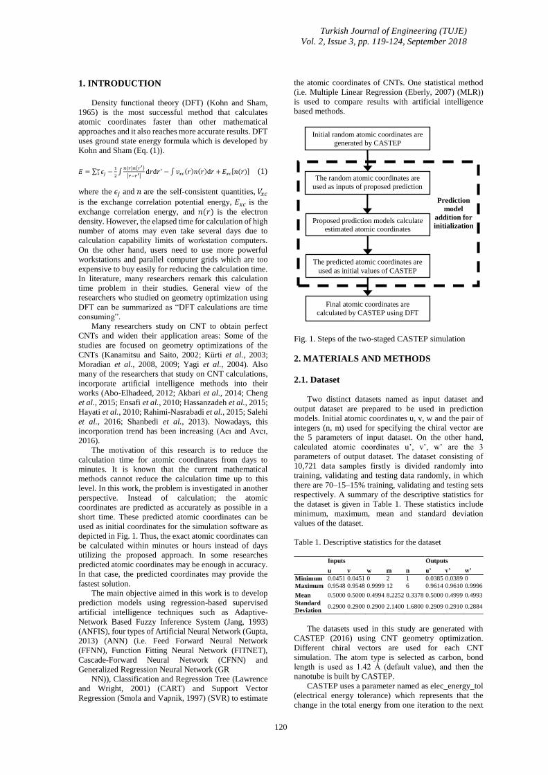
Turkish Journal of Engineering (TUJE)
Vol. 2, Issue 3, pp. 119-124, September 2018
120
1. INTRODUCTION
Density functional theory (DFT) (Kohn and Sham,
1965) is the most successful method that calculates
atomic coordinates faster than other mathematical
approaches and it also reaches more accurate results. DFT
uses ground state energy formula which is developed by
Kohn and Sham (Eq. (1)).
𝐸 = ∑ 𝜖𝑗𝑣1 −
1
2∫
𝑛(𝑟)𝑛(𝑟′)
|𝑟−𝑟′|d𝑟d𝑟′ − ∫ 𝑣𝑥𝑐(𝑟)𝑛(𝑟)d𝑟 + 𝐸𝑥𝑐[𝑛(𝑟)] (1)
where the 𝜖𝑗 and 𝑛 are the self-consistent quantities, 𝑉𝑥𝑐
is the exchange correlation potential energy, 𝐸𝑥𝑐 is the
exchange correlation energy, and 𝑛(𝑟) is the electron
density. However, the elapsed time for calculation of high
number of atoms may even take several days due to
calculation capability limits of workstation computers.
On the other hand, users need to use more powerful
workstations and parallel computer grids which are too
expensive to buy easily for reducing the calculation time.
In literature, many researchers remark this calculation
time problem in their studies. General view of the
researchers who studied on geometry optimization using
DFT can be summarized as “DFT calculations are time
consuming”.
Many researchers study on CNT to obtain perfect
CNTs and widen their application areas: Some of the
studies are focused on geometry optimizations of the
CNTs (Kanamitsu and Saito, 2002; Kürti et al., 2003;
Moradian et al., 2008, 2009; Yagi et al., 2004). Also
many of the researchers that study on CNT calculations,
incorporate artificial intelligence methods into their
works (Abo-Elhadeed, 2012; Akbari et al., 2014; Cheng
et al., 2015; Ensafi et al., 2010; Hassanzadeh et al., 2015;
Hayati et al., 2010; Rahimi-Nasrabadi et al., 2015; Salehi
et al., 2016; Shanbedi et al., 2013). Nowadays, this
incorporation trend has been increasing (Acı and Avcı,
2016).
The motivation of this research is to reduce the
calculation time for atomic coordinates from days to
minutes. It is known that the current mathematical
methods cannot reduce the calculation time up to this
level. In this work, the problem is investigated in another
perspective. Instead of calculation; the atomic
coordinates are predicted as accurately as possible in a
short time. These predicted atomic coordinates can be
used as initial coordinates for the simulation software as
depicted in Fig. 1. Thus, the exact atomic coordinates can
be calculated within minutes or hours instead of days
utilizing the proposed approach. In some researches
predicted atomic coordinates may be enough in accuracy.
In that case, the predicted coordinates may provide the
fastest solution.
The main objective aimed in this work is to develop
prediction models using regression-based supervised
artificial intelligence techniques such as Adaptive-
Network Based Fuzzy Inference System (Jang, 1993)
(ANFIS), four types of Artificial Neural Network (Gupta,
2013) (ANN) (i.e. Feed Forward Neural Network
(FFNN), Function Fitting Neural Network (FITNET),
Cascade-Forward Neural Network (CFNN) and
Generalized Regression Neural Network (GR
NN)), Classification and Regression Tree (Lawrence
and Wright, 2001) (CART) and Support Vector
Regression (Smola and Vapnik, 1997) (SVR) to estimate
the atomic coordinates of CNTs. One statistical method
(i.e. Multiple Linear Regression (Eberly, 2007) (MLR))
is used to compare results with artificial intelligence
based methods.
Fig. 1. Steps of the two-staged CASTEP simulation
2. MATERIALS AND METHODS
2.1. Dataset
Two distinct datasets named as input dataset and
output dataset are prepared to be used in prediction
models. Initial atomic coordinates u, v, w and the pair of
integers (n, m) used for specifying the chiral vector are
the 5 parameters of input dataset. On the other hand,
calculated atomic coordinates u’, v’, w’ are the 3
parameters of output dataset. The dataset consisting of
10,721 data samples firstly is divided randomly into
training, validating and testing data randomly, in which
there are 70–15–15% training, validating and testing sets
respectively. A summary of the descriptive statistics for
the dataset is given in Table 1. These statistics include
minimum, maximum, mean and standard deviation
values of the dataset.
Table 1. Descriptive statistics for the dataset
Inputs Outputs
u v w m n u’ v’ w’
Minimum 0.0451 0.0451 0 2 1 0.0385 0.0389 0
Maximum 0.9548 0.9548 0.9999 12 6 0.9614 0.9610 0.9996
Mean 0.5000 0.5000 0.4994 8.2252 0.3378 0.5000 0.4999 0.4993
Standard
Deviation 0.2900 0.2900 0.2900 2.1400 1.6800 0.2909 0.2910 0.2884
The datasets used in this study are generated with
CASTEP (2016) using CNT geometry optimization.
Different chiral vectors are used for each CNT
simulation. The atom type is selected as carbon, bond
length is used as 1.42 Å (default value), and then the
nanotube is built by CASTEP.
CASTEP uses a parameter named as elec_energy_tol
(electrical energy tolerance) which represents that the
change in the total energy from one iteration to the next
Initial random atomic coordinates are
generated by CASTEP
The random atomic coordinates are
used as inputs of proposed prediction models
Proposed prediction models calculate
estimated atomic coordinates
Final atomic coordinates are
calculated by CASTEP using DFT
The predicted atomic coordinates are
used as initial values of CASTEP
Prediction
model
addition for
initialization
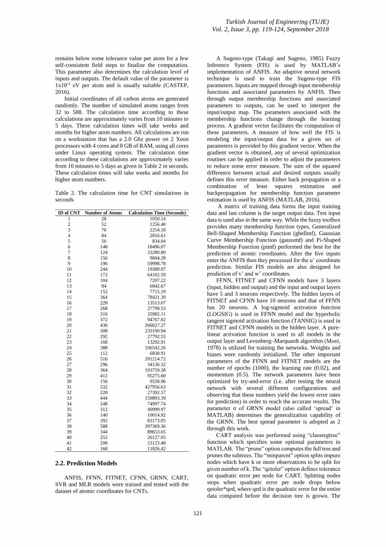
Turkish Journal of Engineering (TUJE)
Vol. 2, Issue 3, pp. 119-124, September 2018
121
remains below some tolerance value per atom for a few
self-consistent field steps to finalize the computation.
This parameter also determines the calculation level of
inputs and outputs. The default value of the parameter is
1x10⁻⁵ eV per atom and is usually suitable (CASTEP,
2016).
Initial coordinates of all carbon atoms are generated
randomly. The number of simulated atoms ranges from
32 to 588. The calculation time according to these
calculations are approximately varies from 10 minutes to
5 days. These calculation times will take weeks and
months for higher atom numbers. All calculations are run
on a workstation that has a 2.0 Ghz power on 2 Xeon
processors with 4 cores and 8 GB of RAM, using all cores
under Linux operating system. The calculation time
according to these calculations are approximately varies
from 10 minutes to 5 days as given in Table 2 in seconds.
These calculation times will take weeks and months for
higher atom numbers.
Table 2. The calculation time for CNT simulations in
seconds
ID of CNT Number of Atoms Calculation Time (Seconds)
1 28 1050.14 2 52 1256.40
3 76 2254.18
4 84 2816.61
5 56 834.04
6 148 18496.07
7 124 33280.80
8 156 9604.28 9 196 59998.78
10 244 19389.07
11 172 64102.59
12 104 7207.22
13 84 6842.67
14 152 7715.19
15 364 78421.39
16 228 13513.07 17 268 27799.53
18 316 35982.11
19 372 94767.02
20 436 266027.27
21 508 233190.94
22 292 27792.55
23 168 13292.91
24 388 106542.26 25 112 6838.91
26 516 201214.72
27 296 34136.32
28 364 103759.38
29 412 95275.60
30 156 9558.96
31 532 427956.63 32 228 27392.57
33 444 159893.39
34 248 74997.74
35 312 40999.97
36 140 10014.92
37 392 83173.05
38 588 397369.36
39 344 89653.65 40 252 26127.05
41 208 23123.48
42 168 11826.42
2.2. Prediction Models
ANFIS, FFNN, FITNET, CFNN, GRNN, CART,
SVR and MLR models were trained and tested with the
dataset of atomic coordinates for CNTs.
A Sugeno-type (Takagi and Sugeno, 1985) Fuzzy
Inference System (FIS) is used by MATLAB’s
implementation of ANFIS. An adaptive neural network
technique is used to train the Sugeno-type FIS
parameters. Inputs are mapped through input membership
functions and associated parameters by ANFIS. Then
through output membership functions and associated
parameters to outputs, can be used to interpret the
input/output map. The parameters associated with the
membership functions change through the learning
process. A gradient vector facilitates the computation of
these parameters. A measure of how well the FIS is
modeling the input/output data for a given set of
parameters is provided by this gradient vector. When the
gradient vector is obtained, any of several optimization
routines can be applied in order to adjust the parameters
to reduce some error measure. The sum of the squared
difference between actual and desired outputs usually
defines this error measure. Either back propagation or a
combination of least squares estimation and
backpropagation for membership function parameter
estimation is used by ANFIS (MATLAB, 2016).
A matrix of training data forms the input training
data and last column is the target output data. Test input
data is used also in the same way. While the fuzzy toolbox
provides many membership function types, Generalized
Bell-Shaped Membership Function (gbellmf), Gaussian
Curve Membership Function (gaussmf) and Pi-Shaped
Membership Function (pimf) performed the best for the
prediction of atomic coordinates. After the five inputs
enter the ANFIS then they processed for the u’ coordinate
prediction. Similar FIS models are also designed for
prediction of v’ and w’ coordinates.
FFNN, FITNET and CFNN models have 3 layers
(input, hidden and output) and the input and output layers
have 5 and 3 neurons respectively. The hidden layers of
FITNET and CFNN have 10 neurons and that of FFNN
has 20 neurons. A log-sigmoid activation function
(LOGSIG) is used in FFNN model and the hyperbolic
tangent sigmoid activation function (TANSIG) is used in
FITNET and CFNN models in the hidden layer. A pure-
linear activation function is used in all models in the
output layer and Levenberg–Marquardt algorithm (Moré,
1978) is utilized for training the networks. Weights and
biases were randomly initialized. The other important
parameters of the FFNN and FITNET models are the
number of epochs (1000), the learning rate (0.02), and
momentum (0.5). The network parameters have been
optimized by try-and-error (i.e. after testing the neural
network with several different configurations and
observing that these numbers yield the lowest error rates
for prediction) in order to reach the accurate results. The
parameter σ of GRNN model (also called ‘spread’ in
MATLAB) determines the generalization capability of
the GRNN. The best spread parameter is adopted as 2
through this work.
CART analysis was performed using “classregtree”
function which specifies some optional parameters in
MATLAB. The “prune” option computes the full tree and
prunes the subtrees. The “minparent” option splits impure
nodes which have k or more observations to be split for
given number of k. The “qetoler” option defines tolerance
on quadratic error per node for CART. Splitting nodes
stops when quadratic error per node drops below
qetoler*qed, where qed is the quadratic error for the entire
data computed before the decision tree is grown. The

Turkish Journal of Engineering (TUJE)
Vol. 2, Issue 3, pp. 119-124, September 2018
122
“mergeleaves” option merges leaves that originate from
the same parent node and give the sum of risk values
greater or equal to the risk associated with the parent
node. The values of the parameters were chosen as
prune=on, minparent=50 (default is 10), qetoler=1E-7
(default is 1E-6), mergeleaves=on. All of the parameter
values were decided by trial-and-error.
SVR model was designed by running “fitrsvm”
function in MATLAB. Several combinations have been
tried and Radial Basis Function was chosen as the kernel
for performance comparison.
MLR prediction model is designed with the purpose
of comparing Machine Learning methods with a
statistical regression method. The model is coded in
Statistics and Machine Learning Toolbox of MATLAB
using “fitlm” function. Model specification is specified as
“linear” and model specification equations are set for
each coordinate for the predictions of coordinates such as
‘u’ ~ u+v+w+m+n’ is set for u’; ‘v’ ~ u+v+w+m+n’ is set
for v’; and ‘w’ ~ u+v+w+m+n’ is set for w’.
3. RESULTS AND DISCUSSION
Mean Squared Error (MSE), Mean Absolute Error
(MAE), Standard Error of Estimation (SEE) and Multiple
Correlation Coefficient (R) are calculated to evaluate the
performance of prediction models. Summaries of
mathematic equations of these performance measures are
given in Eq. (2), Eq. (3), Eq. (4) and Eq. (5) respectively
(Witten and Frank, 2005).
𝑀𝑆𝐸 =1
𝑛[∑ (𝑂𝑖 − 𝑃𝑖)2𝑛
𝑖=1 ] (2)
𝑀𝐴𝐸 =1
𝑛∑ |𝑂𝑖 − 𝑃𝑖|𝑛
𝑖=1 (3)
𝑆𝐸𝐸 = √1 −∑ (𝑂𝑖−𝑃𝑖)2𝑛
𝑖=1
𝑛 (4)
𝑅 = √1 −∑ (𝑂𝑖−𝑃𝑖)2𝑛
𝑖=1
∑ (𝑂𝑖−𝑂𝑚)2𝑛𝑖=1
(5)
where 𝑛 is the number of data points used for testing, 𝑃𝑖
is the predicted value, 𝑂𝑖 is the observed value and 𝑂𝑚 is
the average of the observed values. MATLAB (R2015b
64 bit) (MATLAB, 2016) was utilized for designing
proposed models and obtaining performance measures.
Table 3, Table 4 and Table 5 summarize the
performance results of u’, v’ and w’ coordinates
prediction using ANFIS, FFNN, FITNET, CFNN,
GRNN, SVR, CART and MLR models respectively.
Table 3. Performance results of u’ coordinate prediction
(the best results are outlined in bold).
Models
Performance metrics
MSE MAE SEE R
ANFIS 1.077E-05 2.224E-03 3.282E-03 9.999E-01
FFNN 9.879E-06 2.084E-03 1.000E+00 9.999E-01
FITNET 1.130E-05 2.143E-03 1.000E+00 9.999E-01
CFNN 9.403E-06 2.025E-03 1.000E+00 9.999E-01
GRNN 7.911E-03 2.532E-01 1.000E+00 9.371E-01
SVR 5.102E-04 1.957E-02 9.998E-01 9.970E-01
CART 2.471E-05 3.868E-03 1.000E+00 9.999E-01
MLR 1.525E-01 2.482E+00 3.000E+00 5.999E-01
Table 4. Performance results of v’ coordinate prediction
(the best results are outlined in bold).
Models
Performance Metrics
MSE MAE SEE R
ANFIS 1.101E-05 2.294E-03 3.318E-03 9.999E-01
FFNN 7.307E-06 1.870E-03 1.000E+00 9.999E-01
FITNET 8.708E-06 1.997E-03 1.000E+00 9.999E-01
CFNN 8.537E-06 1.965E-03 1.000E+00 9.999E-01
GRNN 7.995E-03 2.554E-01 1.000E+00 9.298E-01 SVR 4.985E-04 1.940E-02 9.998E-01 9.971E-01
CART 2.484E-05 3.835E-03 1.000E+00 9.998E-01
MLR 1.298E-01 2.300E+00 3.000E+00 6.000E-01
Table 5. Performance results of w’ coordinate prediction
(the best results are outlined in bold).
Models
Performance Metrics
MSE MAE SEE R
ANFIS 4.962E-08 1.534E-04 2.228E-04 1.000E+00
FFNN 5.501E-08 1.531E-04 1.000E+00 1.000E+00
FITNET 5.554E-08 1.523E-04 1.000E+00 1.000E+00
CFNN 5.418E-08 1.498E-04 1.000E+00 1.000E+00
GRNN 8.088E-03 2.466E-01 9.587E-01 9.313E-01 SVR 4.321E-04 1.832E-02 9.997E-01 9.983E-01
CART 2.140E-05 3.021E-03 1.000E+00 9.999E-01
MLR 4.865E-02 1.476E-01 3.000E+00 6.000E-01
All models performed good levels of successes when
we look at all results with a general view. However, the
results of ANFIS, FFNN, FITNET and CFNN models
have a superiority over other models. This implies that
ANN based models can closely estimate atomic
coordinates of CNTs. CART and SVR models produced
average performance results comparing to other models.
The results can be analyzed in detail as follows:
CFNN model has the best performance values for u’
and w’ coordinates prediction by means of MSE and
MAE. However, MSE and R results of ANFIS, FFNN
and FITNET models are very close to CFNN model.
The best SEE results are achieved by ANFIS model for
all coordinates.
R value prediction results varies in a very small range
(from 9.298E-01 to 1.000E+00) for all models except
MLR based model.
MLR based model yielded the worst performance
results for all coordinates.
The estimation results with the highest accuracy are
yielded for w' coordinate (MSE results of the first four
models are almost zero).
The results obtained from this study can be used in
two ways: i) The predicted atomic coordinates can be
used in physical calculations without using a simulation
software, ii) The estimated results can be used as an initial
value of simulation software for reducing duration of the
atomic coordinate calculation seriously.
4. CONCLUSION
As a result of this work, the effectiveness of artificial
intelligence based solutions, which estimate atomic
coordinates that can be integrated into software, has been
observed and the results that have significantly shortened
the simulation processes in the field of nanotechnology
have been presented to be integrated into scientific or
commercial software.
Turkish Journal of Engineering (TUJE)
Vol. 2, Issue 3, pp. 119-124, September 2018
123
ACKNOWLEDGMENTS
We would like to thank Çukurova University
Scientific Research Projects Center for supporting this
work (Project code: FDK-2015-3170).
REFERENCES
Abo-Elhadeed, A. F. (2012). "Modeling carbon nanotube
transistors using neural networks approach." Proc.,
International Conference on Synthesis, Modeling,
Analysis and Simulation Methods and Applications to
Circuit Design (SMACD), pp. 125-128.
Acı, M. and Avcı, M. (2016). "Artificial neural network
approach for atomic coordinate prediction of carbon
nanotubes." Applied Physics A, vol. 7 No. 122, pp. 1-14.
Akbari, E., Buntat, Z., Enzevaee, A., Ebrahimi, M.,
Yazdavar, A. H. and Yusof, R. (2014). "Analytical
modeling and simulation of I–V characteristics in carbon
nanotube based gas sensors using ANN and SVR
methods." Chemometrics and Intelligent Laboratory
Systems, Vol. 137, No. 1, pp. 173-180.
CASTEP Biovia Materials. http://accelrys.com/products/
collaborative-science/biovia-materials-studio/quantom-
catalysis-software.html [Accessed 10 May 2017].
Cheng, W., Cai, C., Luo, Y., Li, Y. and Zhao, C. (2015).
"Mechanical properties prediction for carbon
nanotubes/epoxy composites by using support vector
regression." Modern Physics Letters B, Vol. 29, No. 05,
pp. 1550016.
Eberly, L. E. (2007). Multiple linear regression. In:
Topics in biostatistics, Humana Press, Totowa, NJ, USA.
Ensafi, A. A., Taei, M., Khayamian, T. and Hasanpour,
F. (2010). "Simultaneous voltammetric determination of
enrofloxacin and ciprofloxacin in urine and plasma using
multiwall carbon nanotubes modified glassy carbon
electrode by least-squares support vector machines."
Analytical Sciences, Vol. 26, No. 7, pp. 803-808.
Gupta, N. (2013). "Artificial neural network." Network
and Complex Systems, Vol. 3, No. 1, pp. 24-28.
Hassanzadeh, Z., Kompany-Zareh, M., Ghavami, R.,
Gholami, S. and Malek-Khatabi, A. (2015). "Combining
radial basis function neural network with genetic
algorithm to QSPR modeling of adsorption on multi-
walled carbon nanotubes surface." Journal of Molecular
Structure, Vol. 1098, No. 1, pp. 191-198.
Hayati, M., Rezaei, A. and Seifi, M. (2010). "CNT-
MOSFET modeling based on artificial neural network:
Application to simulation of nanoscale circuits." Solid-
State Electronics, Vol. 54, No. 1, pp. 52-57.
Jang, J.-S. (1993). "ANFIS: adaptive-network-based
fuzzy inference system." IEEE Transactions on Systems,
Man, and Cybernetics, Vol. 23, No. 3, pp. 665-685.
Kanamitsu, K. and Saito, S. (2002). "Geometries,
electronic properties, and energetics of isolated single
walled carbon nanotubes." Journal of the Physical
Society of Japan, Vol. 71, No. 2, pp. 483-486.
Kohn, W. and Sham, L. J. (1965). "Self-consistent
equations including exchange and correlation effects."
Physical review, Vol. 140, No. 4A, pp. A1133–A1138.
Kürti, J., Zólyomi, V., Kertesz, M. and Sun, G. (2003).
"The geometry and the radial breathing mode of carbon
nanotubes: beyond the ideal behaviour." New Journal of
Physics, Vol. 5, No. 1, pp. 125.
Lawrence, R. L. and Wright, A. (2001). "Rule-based
classification systems using classification and regression
tree (CART) analysis." Photogrammetric Engineering
and Remote sensing, Vol. 67, No. 10, pp. 1137-1142.
MATLAB. https://www.mathworks.com/ [Accessed 12
May 2017].
Moradian, R., Behzad, S. and Chegel, R. (2008). "Ab
initio density functional theory investigation of structural
and electronic properties of silicon carbide nanotube
bundles." Physica B: Condensed Matter, Vol. 403, No.
19, pp. 3623-3626.
Moradian, R., Behzad, S. and Chegel, R. (2009). "Ab
initio density functional theory investigation of Li-
intercalated silicon carbide nanotube bundles." Physics
Letters A, Vol. 373, No. 26, pp. 2260-2266.
Moré J.J. (1978). The levenberg-marquardt algorithm:
implementation and theory. In: Numerical analysis,
Springer, Berlin, Germany.
Rahimi-Nasrabadi, M., Akhoondi, R., Pourmortazavi, S.
M. and Ahmadi, F. (2015). "Predicting adsorption of
aromatic compounds by carbon nanotubes based on
quantitative structure property relationship principles."
Journal of Molecular Structure, Vol. 1099, No. 1, pp.
510-515.
Salehi, E., Abdi, J. and Aliei, M. H. (2016). "Assessment
of Cu (II) adsorption from water on modified membrane
adsorbents using LS-SVM intelligent approach." Journal
of Saudi Chemical Society, Vol. 20, No. 2, pp. 213-219.
Shanbedi, M., Jafari, D., Amiri, A., Heris, S. Z. and
Baniadam, M. (2013). "Prediction of temperature
performance of a two-phase closed thermosyphon using
artificial neural network." Heat and Mass Transfer, Vol.
49, No. 1, pp. 65-73.
Smola, A. and Vapnik, V. (1997). "Support vector
regression machines." Advances in Neural Information
Processing Systems, Vol. 9, No. 1, pp. 155-161.
Takagi, T. and Sugeno, M. (1985). "Fuzzy identification
of systems and its applications to modeling and control."
IEEE Transactions on Systems, Man, and Cybernetics,
Vol. SMC-15, No. 1, pp. 116-132.

Turkish Journal of Engineering (TUJE)
Vol. 2, Issue 3, pp. 119-124, September 2018
124
Witten, I. H. and Frank, E. (2005). Data mining: practical
machine learning tools and techniques, Morgan
Kaufmann, San Francisco, USA.
Yagi, Y., Briere, T. M., Sluiter, M. H., Kumar, V.,
Farajian, A. A. and Kawazoe, Y. (2004). "Stable
geometries and magnetic properties of single-walled
carbon nanotubes doped with 3 d transition metals: A
first-principles study." Physical Review B, Vol. 69, No. 7, pp. 075414.
Copyright © Turkish Journal of Engineering (TUJE).
All rights reserved, including the making of copies
unless permission is obtained from the copyright
proprietors.
Turkish Journal of Engineering
125
Turkish Journal of Engineering (TUJE)
Vol. 2, Issue 3, pp. 125-129, September 2018
ISSN 2587-1366, Turkey
DOI: 10.31127/tuje.403215
Research Article
INVESTIGATION OF ULEXITE USAGE IN AUTOMOTIVE BRAKE FRICTION
MATERIALS
Banu Sugözü *1
Mersin University, Faculty of Engineering, Department of Mechanical Engineering, Mersin, Turkey
ORCID ID 0000-0002-7798-2677
* Corresponding Author
Received: 08/03/2018 Accepted: 04/05/2018
ABSTRACT
The automotive brake pads are multi-component composites made up of many materials. There are many studies in the
literature exploring the use of many different materials in brake pads. In this study, the use of ulexite which is a
commercially valuable derivatives of boron that 65% of the total world reservations exists in Turkey were researched for
brake pad material. For this purpose, three brake pad specimens containing ulexite differing in amount (3, 6 and 9 wt.%)
were produced by a conventional procedure for a dry formulation following dry-mixing, pre-forming and hot pressing. The
density of the specimens was determined based on Archimedes principle in water. The surface hardness of all brake pad
specimens was measured using Rockwell hardness tester. The friction performance of the brake pad specimens was
determined using a real brake disc-type tester with grey cast iron. The weights of each specimen were taken before and
after the friction test, and the specific wear rate was determined in accordance to the TSE 555 (1992) standard. The results
showed that all specimens are applicable to the industry, consistent with the literature and suitable to the TS 555 standard.
Also, the results indicated that ulexite is an ideal material for brake pads.
Keywords: Ulexite, Brake Lining, Wear, Friction
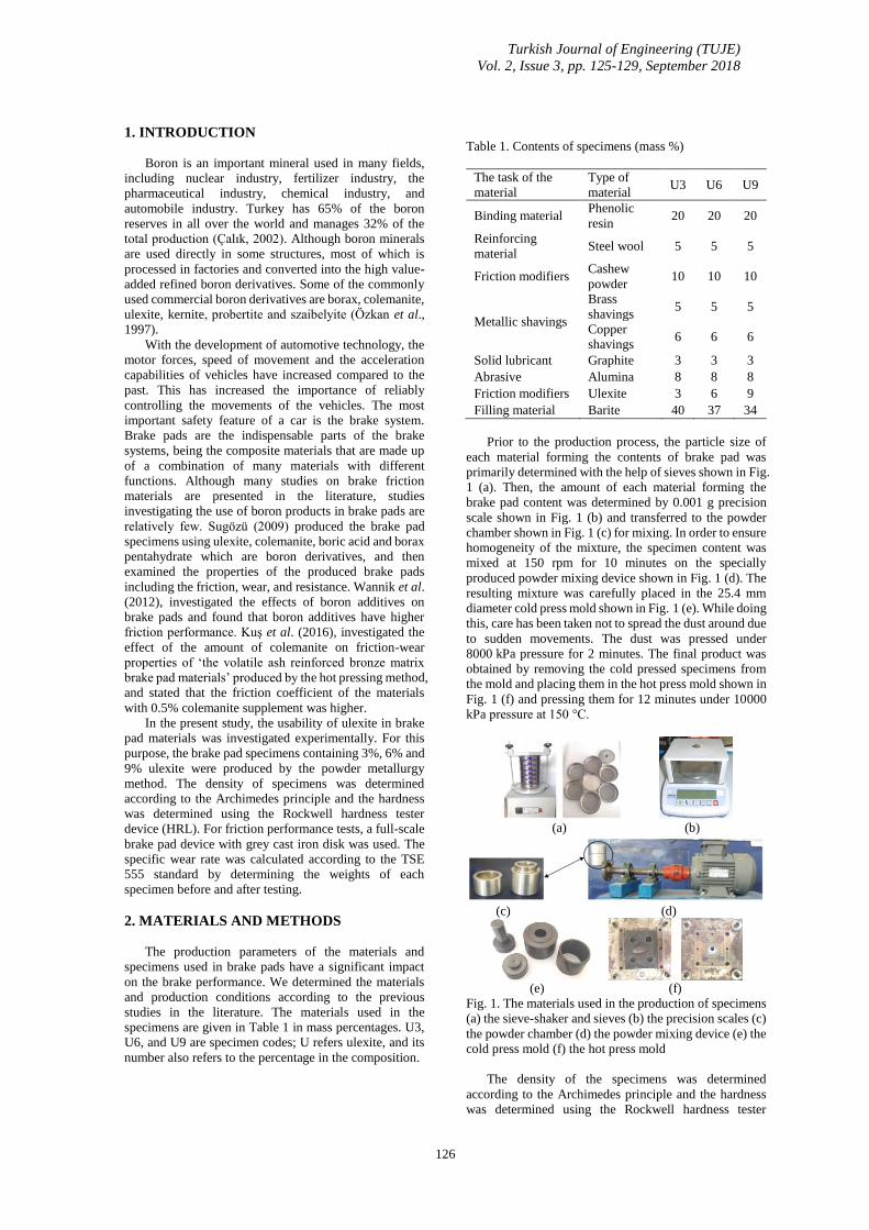
Turkish Journal of Engineering (TUJE)
Vol. 2, Issue 3, pp. 125-129, September 2018
126
1. INTRODUCTION
Boron is an important mineral used in many fields,
including nuclear industry, fertilizer industry, the
pharmaceutical industry, chemical industry, and
automobile industry. Turkey has 65% of the boron
reserves in all over the world and manages 32% of the
total production (Çalık, 2002). Although boron minerals
are used directly in some structures, most of which is
processed in factories and converted into the high value-
added refined boron derivatives. Some of the commonly
used commercial boron derivatives are borax, colemanite,
ulexite, kernite, probertite and szaibelyite (Özkan et al.,
1997).
With the development of automotive technology, the
motor forces, speed of movement and the acceleration
capabilities of vehicles have increased compared to the
past. This has increased the importance of reliably
controlling the movements of the vehicles. The most
important safety feature of a car is the brake system.
Brake pads are the indispensable parts of the brake
systems, being the composite materials that are made up
of a combination of many materials with different
functions. Although many studies on brake friction
materials are presented in the literature, studies
investigating the use of boron products in brake pads are
relatively few. Sugözü (2009) produced the brake pad
specimens using ulexite, colemanite, boric acid and borax
pentahydrate which are boron derivatives, and then
examined the properties of the produced brake pads
including the friction, wear, and resistance. Wannik et al.
(2012), investigated the effects of boron additives on
brake pads and found that boron additives have higher
friction performance. Kuş et al. (2016), investigated the
effect of the amount of colemanite on friction-wear
properties of ‘the volatile ash reinforced bronze matrix
brake pad materials’ produced by the hot pressing method,
and stated that the friction coefficient of the materials
with 0.5% colemanite supplement was higher.
In the present study, the usability of ulexite in brake
pad materials was investigated experimentally. For this
purpose, the brake pad specimens containing 3%, 6% and
9% ulexite were produced by the powder metallurgy
method. The density of specimens was determined
according to the Archimedes principle and the hardness
was determined using the Rockwell hardness tester
device (HRL). For friction performance tests, a full-scale
brake pad device with grey cast iron disk was used. The
specific wear rate was calculated according to the TSE
555 standard by determining the weights of each
specimen before and after testing.
2. MATERIALS AND METHODS
The production parameters of the materials and
specimens used in brake pads have a significant impact
on the brake performance. We determined the materials
and production conditions according to the previous
studies in the literature. The materials used in the
specimens are given in Table 1 in mass percentages. U3,
U6, and U9 are specimen codes; U refers ulexite, and its
number also refers to the percentage in the composition.
Table 1. Contents of specimens (mass %)
The task of the
material
Type of
material U3 U6 U9
Binding material Phenolic
resin 20 20 20
Reinforcing
material Steel wool 5 5 5
Friction modifiers Cashew
powder 10 10 10
Metallic shavings
Brass
shavings 5 5 5
Copper
shavings 6 6 6
Solid lubricant Graphite 3 3 3
Abrasive Alumina 8 8 8
Friction modifiers Ulexite 3 6 9
Filling material Barite 40 37 34
Prior to the production process, the particle size of
each material forming the contents of brake pad was
primarily determined with the help of sieves shown in Fig.
1 (a). Then, the amount of each material forming the
brake pad content was determined by 0.001 g precision
scale shown in Fig. 1 (b) and transferred to the powder
chamber shown in Fig. 1 (c) for mixing. In order to ensure
homogeneity of the mixture, the specimen content was
mixed at 150 rpm for 10 minutes on the specially
produced powder mixing device shown in Fig. 1 (d). The
resulting mixture was carefully placed in the 25.4 mm
diameter cold press mold shown in Fig. 1 (e). While doing
this, care has been taken not to spread the dust around due
to sudden movements. The dust was pressed under
8000 kPa pressure for 2 minutes. The final product was
obtained by removing the cold pressed specimens from
the mold and placing them in the hot press mold shown in
Fig. 1 (f) and pressing them for 12 minutes under 10000
kPa pressure at 150 °C.
(a) (b)
(c) (d)
(e) (f)
Fig. 1. The materials used in the production of specimens
(a) the sieve-shaker and sieves (b) the precision scales (c)
the powder chamber (d) the powder mixing device (e) the
cold press mold (f) the hot press mold
The density of the specimens was determined
according to the Archimedes principle and the hardness
was determined using the Rockwell hardness tester

Turkish Journal of Engineering (TUJE)
Vol. 2, Issue 3, pp. 125-129, September 2018
127
device (HRL). During the hardness measurement process,
a preload of 10 kgf and a full load of 60 kgf was applied
with a steel ball in diameter 6.35 mm at the submersible
end (Başar et al., 2017). Hardness measurements were
taken from the frictional surface of the specimens. A full-
scale brake pad test device with grey cast iron disc having
a diameter of 280 mm and hardness of 116 HB, whose
schematic drawing is shown in Fig. 2, was used to
determine the abrasion and friction properties of the
specimens. The device can be fully controlled by a
computer and includes data collection software. The
specific wear rate was calculated according to the TSE
555 standard by determining the weights of each
specimen before and after testing.
During the experiments, the temperature increases
due to friction between the disk and the brake pad. In
order to investigate the effect of temperature increase on
the performance of the brake pad, the non-contact
thermometer measured the surface temperature of the
brake pad at a distance of about 2 cm from the friction
surface to the disc. A digital thermometer was used to
measure temperature. The surface temperature of the disc
is automatically transferred to the computer environment
in seconds during the experiment (Sugözü, 2016).
Fig. 2. Brake pad test device (Sugözü, 2015)
The coefficient of friction and wear of specimens was
obtained by conducting experiments as specified in the
TS 555 (1992) and TS 9076 standard (1991). In
experimental conditions, first of all, 310 rpm, 700 kPa
pressure, and a temperature not exceeding 100 °C were
provided; and then the grinding process was applied, until
the surface contact of the specimen to the disc is at least
95%. Thus, the surface got ready for the experiment. Then
the tests were completed with the pressure of 1050 kPa
and speed of 6 m/s for 30 minutes.
3. RESULTS
The coefficient of friction for automotive brake pads
is the most important parameter affecting the brake
performance. The coefficient of friction-temperature-
time graphs of specimens are given in Fig. 3 for U3 coded
specimens, and in Fig. 4 for U6 coded specimens, and
also in Fig. 5 for U9 coded specimens. In figures, the
coefficient of friction was low at the initial of the test
because the applied pressure does not influence suddenly
but gradually. Sudden pressure application will cause
damage to the brake pads, so the pressure was gradually
increased. In addition, at the initial of the test, the disc and
the brake pad are in the running-in period (grinding) and
the friction layers in which the friction force is effective
are not yet formed (Sugözü, 2016). Therefore, there is a
continuous change in the coefficient of friction. In the
literature, this situation has been reported to occur with
the transition of heat to the inner part of the contact areas
on the surface of the disc during friction (Anderson, 1992).
Another explication is that the adhesion on the surface
roughness of the friction couples results in the repetition
of the adhesion-release, causing fluctuations in the
coefficient of friction (Stachowiak and Batchelor, 2001).
Fig. 3. The coefficient of friction and temperature graph
of the specimen containing 3% ulexite, according to the
friction time
Fig. 4. The coefficient of friction and temperature graph
of the specimen containing 6% ulexite, according to the
friction time
Fig. 5. The coefficient of friction and temperature graph
of the specimen containing 9% ulexite, according to the
friction time
Fig. 3 shows the coefficient of friction and
temperature graph of the specimen containing 3% ulexite,
according to the friction time. The highest coefficient of
friction obtained during the tests was 0.47, and the highest
temperature was 206.8 °C. Fig. 4 shows the coefficient of
friction and temperature graph of the specimens
containing 6% ulexite, according to the friction time.
During the tests, the highest temperature occurred
between the disk and brake pad is 193.3 °C. The highest
coefficient of friction of the brake pad specimen is 0.44.
However, the friction stability was found to be 71%. Fig.

Turkish Journal of Engineering (TUJE)
Vol. 2, Issue 3, pp. 125-129, September 2018
128
5 represents the coefficient of friction and temperature
graph of the specimen containing 9% ulexite. The highest
coefficient of friction obtained in the tests is 0.48 °C, and
the highest temperature between the disc and brake pad is
202 ° C. The friction stability was calculated as 70%.
According to the literature, the friction stability (%)
should be as high as possible and close to 100, the slope
and fluctuations of the obtained curve should be low level
(Bijwe et al., 2012). It is desirable that the coefficient of
friction of the automotive brake pads is high, the wear is
low and the friction stability is stable. Physical and
tribological properties of specimens are shown in Table 2
and Table 3.
Table 2. Tribological properties of specimens
Specimen
Code
Specific wear
rate (cm3/Nm)
The average
coefficient of friction
U3 2.054 × 10⁻⁶ 0.331
U6 2.109 × 10⁻⁶ 0.313
U9 1.893 × 10⁻⁶ 0.337
Table 3. Physical properties of specimens
Specimen
Code
Rockwell
hardness (HRL)
Density
(g/cm3)
U3 81 1.9
U6 88 2.16
U9 90 2.22
Table 3 shows that the hardness and density of the
specimens are increased by increasing the amount of
ulexite in the composite. Considering the average
coefficient of friction and the specific wear rate, it was
found that the specimen containing 9% ulexite was better.
The coefficient of friction of the specimens is obtained by
dividing the coefficient of friction by the highest
coefficient of friction obtained during the test and
expressed as a percentage.
(a) (b)
Fig. 6. (a) The coefficient of friction (b) friction stability
graphs of specimens
4. CONCLUSION
In this study, the usability of ulexite, which is a boron
mineral, in automotive brake pads was investigated by
experimental studies. Three different specimens
containing 3%, 6% and 9% ulexite were prepared for this
purpose. A full-scale brake pad device was used for the
wear and friction tests of the specimens. The results
obtained from the tests are summarized below;
• The highest average coefficient of friction value for
all specimens undergo friction test is 0.337, belonging to
the U9-coded specimen containing 9% ulexite, the lowest
average friction coefficient is 0.313, belonging to the U6-
coded specimen containing 6% ulexite.
• It was reported that as the amount of ulexite
increased, the hardness and density increased. The direct
proportion between the hardness and density was
determined to be consistent with the literature.
• The friction stability of specimens was observed to
be almost the same for each specimen, and it was
concluded that the friction stability does not depend on
the amount of ulexite content.
• According to the results obtained from the friction
and abrasion tests, all specimens can be utilized in the
industry in accordance with the literature and conform to
the TS 555 standard. Accordingly, ulexite which is a
boron derivative could be used as an alternative material
in automotive brake pads.
REFERENCES
Anderson, A. E. (1992). ASM handbook, Friction,
lubrication, and wear technology 18, pp. 569-577.
Başar, G., Buldum, B.B., Sugözü, İ. (2017). “Effects of
Colemanite and Ulexite on the Tribological
Characteristics of Brake Friction Materials.” Proc.,
International Advanced Researches & Engineering
Congress, Osmaniye, Turkey, pp. 87-94.
Bijwe, J., Aranganathan, N., Sharma, S., Dureja, N. and
Kumar, R. (2012). “Nano-abrasives in friction materials-
influence on tribological properties.” Wear, Vol. 296,
No. 1, pp. 693-701.
Çalık, A. (2002). “Turkey boron minerals and features.”
Engineer and Machinery, Vol. 508, pp. 1-9.
Kuş, H., Altıparmak, D. and Başar G. (2016). “The Effect
of Colemanite Content on Friction-Wear Properties of the
Bronze Based Brake Lining Material Reinforced with Fly
Ash Fabricated by the Hot Pressing Method.” Journal of
Polytechnic, Vol. 19, No. 4, pp. 537-546.
Özkan, Ş. G., Çebi, H., Delice, S., and Doğan, M. (1997).
“Boron minerals properties and mining.” Proc., 2nd
Industrial Minerals Symposium, İzmir, Turkey, pp. 224-
228.
Stachowiak, G.W. and Batchelor, A.W. (2001).
Engineering Tribology, Heineman, Boston, MA, pp. 36-
44.
Sugözü, İ. (2009). Production of non-asbestos automotive
brake lining additional boron and investigation of its
braking characteristic, PhD Thesis, Fırat University,
Elazığ, Turkey.
Sugözü, I. (2015). “Investigation of using rice husk dust
and ulexite in automotive brake pads.” Materials Testing,
Vol. 57, No. 10, pp. 877-882.
Sugözü, B. (2016). The effect of additive of nano silica,
nano alumina and nano zircon abrasive particles on brake
lining properties, PhD Thesis, Selçuk University, Konya,
Turkey.
Turkish Journal of Engineering (TUJE)
Vol. 2, Issue 3, pp. 125-129, September 2018
129
TS 555 (1992). Highway Vehicles-Brake System-Brake
Pads for Friction Brake, Turkish Standard Institute,
Ankara, Turkey.
TS 9076 (1991). Road Vehicles-Brake Linings-
Evaluation of Friction Material Characteristics- Small
Sample Bench Test Procedure, Turkish Standard Institute,
Ankara, Turkey.
Wannik, W. B., Ayob, A. F., Syahrullail, S., Masjuki, H.
H. and Ahmad M. F. (2012). “The effect of boron friction
modifier on the performance of brake pads.”
International Journal of Mechanical and Materials
Engineering, Vol. 7, No. 1, pp. 31-35.
Copyright © Turkish Journal of Engineering (TUJE).
All rights reserved, including the making of copies
unless permission is obtained from the copyright
proprietors.
Turkish Journal of Engineering
130
Turkish Journal of Engineering (TUJE)
Vol. 2, Issue 3, pp. 130-138, September 2018
ISSN 2587-1366, Turkey
DOI: 10.31127/tuje.411549
Research Article
CRITICALITY CALCULATION OF A HOMOGENOUS CYLINDRICAL
NUCLEAR REACTOR CORE USING FOUR-GROUP DIFFUSION EQUATIONS
Babatunde Michael Ojo *1, Musibau Keulere Fasasi 2, Ayodeji Olalekan Salau 3, Stephen Friday Olukotun 4 and Mathew
Ademola Jayeola 5
1 Obafemi Awolowo University, Science Faculty, Physics and Engineering Physics Department, Ile-Ife, Nigeria
ORCID ID 0000-0002-2217-7654 [email protected]
2 Obafemi Awolowo University, Science Faculty, Center for Energy and Research Development, Ile-Ife, Nigeria
ORCID ID 0000-0002-4056-173X [email protected]
3 Obafemi Awolowo University, Technology Faculty, Electronic and Electrical Engineering Department, Ile-Ife, Nigeria
ORCID ID 0000-0002-6264-9783 [email protected]
4 Obafemi Awolowo University, Science Faculty, Physics and Engineering Physics Department, Ile-Ife, Nigeria
ORCID ID 0000-0002-7409-5466 [email protected]
5 Obafemi Awolowo University, Science Faculty, Physics and Engineering Physics Department, Ile-Ife, Nigeria
ORCID ID 0000-0002-3131-3187 [email protected]
* Corresponding Author
Received: 01/04/2018 Accepted: 04/05/2018
ABSTRACT
In this study, we present a general equation for Finite Difference Method Multi-group Diffusion (FDMMD) equations of
a cylindrical nuclear reactor core. In addition, we developed an algorithm which we called TUNTOB for solving the
FDMMD equations, determined the fluxes at each of the mesh points and calculated the criticality of the four energy
group. This was with a view to using the four-group diffusion equations to estimate the criticality of a cylindrical reactor
core that will be accurate and locally accessible for nuclear reactor design in developing countries. The multi-group
diffusion equations were solved numerically by discretization using the Finite Difference Method (FDM) to obtain a
general equation for a cylindrical reactor core. The fluxes at each mesh point and the criticality of the four energy group
were then determined. From the results obtained, we observed that an increment in iteration led to an increase in the
effective multiplication factor (𝒌𝒆𝒇𝒇) with a corresponding increase in the computation time. A maximum effective
multiplication factor was reached when the number of iteration was 1000 and above. Having established the optimal
number of iterations, the effects of the mesh sizes on the computation examined revealed that the values of 𝒌𝒆𝒇𝒇
increases as the mesh sizes becomes smaller until an optimal mesh size of 1 x 1 cm2 was reached and further decrease in
mesh sizes gave no further improvement in the value of 𝒌𝒆𝒇𝒇. The Study concluded that the accuracy in the values of
𝒌𝒆𝒇𝒇 and the smoothness of the neutron distribution curves in 3-D representations depend on the number of mesh points.
Keywords: Four-group diffusion equation, Effective multiplication factor, Mesh size, Reactor, Criticality calculation
Turkish Journal of Engineering (TUJE)
Vol. 2, Issue 3, pp. 130-138, September 2018
131
1. INTRODUCTION
The criticality of a system containing fissionable
materials is described by its effective multiplication
factor (𝒌𝒆𝒇𝒇). The effective multiplication factor is the
ratio of the number of neutrons in one generation to the
number of neutrons in the previous generation as shown
in Eq. (𝟏). A generation is essentially the lifetime of a
neutron, in a finite system, the effective multiplication
factor is denoted as 𝒌𝒆𝒇𝒇𝒆𝒄𝒕𝒊𝒗𝒆 or 𝒌𝒆𝒇𝒇, which is used to
determine the stability of a nuclear reactor core. When a
system is critical, it maintains a steady–state chain
reaction of nuclear fissioning, and 𝒌𝒆𝒇𝒇 = 1. The average
neutron population in a critical system stays constant in
time. A sub-critical system has 𝒌𝒆𝒇𝒇 < 1 and the neutron
population dies off in time. The neutron population in a
super-critical system, where 𝒌𝒆𝒇𝒇 > 1, grows without
bound in time (Urbatsch, 1995).
𝒌𝒆𝒇𝒇 = 𝑁𝑢𝑚𝑏𝑒𝑟 𝑜𝑓 𝑛𝑒𝑢𝑡𝑟𝑜𝑛𝑠 𝑖𝑛 𝑜𝑛𝑒 𝑔𝑒𝑛𝑒𝑟𝑎𝑡𝑖𝑜𝑛
𝑁𝑢𝑚𝑏𝑒𝑟 𝑜𝑓 𝑛𝑒𝑢𝑡𝑟𝑜𝑛𝑠 𝑖𝑛 𝑡ℎ𝑒 𝑝𝑟𝑒𝑐𝑒𝑑𝑖𝑛𝑔 𝑔𝑒𝑛𝑒𝑟𝑎𝑡𝑖𝑜𝑛
(1)
The knowledge of 𝒌𝒆𝒇𝒇 is necessary when designing
nuclear reactors. However, numerical methods are used
almost exclusively for criticality calculations (Urbatsch,
1995). Different numerical methods have been proposed
to solve the two group neutron diffusion equations with
little attention to the other groups. Although, the two
group neutron diffusion equations do not give a detailed
explanation of neutron flux distribution in a practical
nuclear reactor core, the four-group neutron diffusion
equations are known to give a far better description of
neutron distribution in a practical nuclear reactor core.
Hence the study of the criticality of the cylindrical
reactor core and its calculation using four-group
diffusion equations by applying the finite difference
method (FDM).
The remainder of this paper is organized as follows.
In Section 2, a review of related works is provided,
while a detailed explanation of the discretization of the
four group diffusion equations using finite difference
method is given in Section 3. In Section 4, the results are
presented and discussed and Section 5 concludes this
paper.
2. NUCLEAR REACTOR CORE
A nuclear reactor core is a part of a nuclear reactor
which contains the nuclear fuel components where all
the nuclear reactions takes place and consequently heat
is generated from the reaction. In addition, a nuclear
reactor produces and controls the release of energy in
form of heat from the splitting of the atoms of uranium.
2.1. Neutron-Nucleus Reactions
It is important to recognize that since neutrons are
electrically neutral, they are unaffected by the electrons
in the atom or by the positive charge of the nucleus. As a
consequence, neutrons pass through the atomic electron
cloud and interact directly with the nucleus. Neutrons
collide with nuclei, not with atoms (Larmash and
Baratta, 2001).
The operation of a reactor basically depends on how
neutrons interact with nuclei in the reactor. There are
various types of known neutron interactions which could
be considered as shown in Fig. 1 (Arzhanov, 2010). All
neutron reactions can be categorized as either elastic or
inelastic collisions, on the condition that either the
kinetic energy is conserved in the collision or not.
(Burnham, 1967).
2.1.1. Neutron Flux
Neutron flux is defined as the product of the neutron
density and the velocity,
𝜙 = 𝑛𝑣 (2)
so that it is expressed in units of neutrons per 𝑐𝑚2 per
second. It is equal to the total distance (sum of all the
path lengths) travelled in one second by all the neutrons
present in one 𝑐𝑚3.
In a reactor, the values of neutron density and
neutron flux are a function of location in the core.
Because the neutron flux is an essential ingredient in the
computation of reactor rates, the determination of the
spatial distribution of the neutron flux in the core is an
important part of reactor physics. The value of the
neutron flux at a given point in the core will depend on
the distribution of nuclear properties like the cross
sections throughout the core, and on the position in
relation to the central part of the core and to the external
surface of the reactor. The neutron flux continually
drops to zero at, or just beyond, the radial and axial
boundaries of the core. The behavior of the flux in the
core and its rate of decline towards the boundaries must
be calculated by means of computer codes (AECBC,
1993; Jayeola et al., 2018).
2.1.2. The Neutron Diffusion Equation
The neutron diffusion equations provide an essential
exact description of the neutron distribution within a
reactor. Its solution would contain essentially all the
information we require concerning the nuclear behavior
of the reactor (Duderstadt and Hamilton, 1976).
The multi-group diffusion equation comprises of the
groups of neutrons of different energies diffusing within
a nuclear reactor. The basic diffusion equation for each
group of neutrons is the same, but with absorption
generalized to all processes that remove the neutron
from the group that is absorption plus scattering to
another group and with the source of neutrons for each
group specialized to include the in-scattering of neutrons
from the other groups, which is also diffusing within the
reactor (Stacey, 2007).
2.1.3. Numerical Methods used in neutron
diffusion equation
It is assumed that a uniform reactor has the shape of
a cylinder of physical radius (R) and height (H). This
finite cylindrical reactor has cylindrical geometry which
have coordinates at its origin. In order to solve the
diffusion equations, the Laplacian is replaced by its
Turkish Journal of Engineering (TUJE)
Vol. 2, Issue 3, pp. 130-138, September 2018
132
cylindrical form: cylindrical coordinates - 3D, 2D. This
is not dependent on angle Θ, therefore, the 3D Laplacian
is replaced by its two-dimensional form (2D). This
makes it practicable to solve the problem using radial
and axial directions. This is because the flux is a
function of radius – r and height – z only (Φ(r, z)).
Furthermore, numerical solutions of neutron
diffusion equations have been solved using a number of
numerical methods such as the finite difference, finite
element, nodal and boundary element methods. These
methods are all mesh-based in which the nodes that
discretize the problem domain are related in a predefined
manner (Tanbay and Bilge, 2013). However, numerical
methods are used most exclusively for criticality
calculations. Criticality calculations 𝒌𝒆𝒇𝒇 are based on
power iteration procedures, where different multi-group
diffusion equations with a number of iterations are used
to estimate the effective multiplication factor ( 𝒌𝒆𝒇𝒇 ).
This iteration process is repeated until the fission
distribution has converged.
3. METHODOLOY
3.1. Calculation of the Four-Group Diffusion
Equations
To calculate the four-group diffusion equation, we
use the finite difference discretization of steady state
four-group neutron diffusion equation in a cylindrical
coordinate. First, the finite difference discretization of
one group differential equation was established and later
extended to four-group differential equation. The
boundary conditions introduced in this research are: the
neutron flux vanishes at the extrapolated boundary of the
core (r = R and z = 0, H). Where R = Extrapolated
Radius and H = Extrapolated Height. The multi-group
diffusion system in a cylindrical coordinate can be
written as:
1
𝑟
𝜕
𝜕𝑟[𝐷(𝑟, 𝑧)𝑟
𝜕𝜑(𝑟, 𝑧)
𝜕𝑟] +
𝜕
𝜕𝑧[𝐷(𝑟, 𝑧)
𝜕𝜑(𝑟, 𝑧)
𝜕𝑧]
− ∑ (𝑟, 𝑧)𝜑(𝑟, 𝑧) 𝑡
= −𝑆(𝑟, 𝑧) (3)
The dependent variable in Eq. (3) is the neutron flux,
D is the diffusion coefficient and S is the neutron fission
source used to initiate the fission reaction. The third
term in Eq. (3), (sigma subscript 't') is the total
macroscopic cross section of the reactor core.
Multiplying Eq. (3) through by r, we obtain:
𝜕
𝜕𝑟[𝐷(𝑟, 𝑧)𝑟
𝜕𝜑(𝑟,𝑧)
𝜕𝑟] +
𝜕
𝜕𝑧[𝑟𝐷(𝑟, 𝑧)
𝜕𝜑(𝑟,𝑧)
𝜕𝑧] −
𝑟 ∑ (𝑟, 𝑧)𝜑(𝑟, 𝑧) 𝒕 = −𝑟𝑆(𝑟, 𝑧) (4)
The Eq. (4) was discretized using a finite difference
method to obtain the four-group diffusion equations by
considering the neutron flux varying along the radial and
axial coordinate, hence the Fick’s law for the radial and
axial coordinate can be written as Eqs. (5) and (6) respectively:
J = 𝐷(𝑟, 𝑧)𝑟𝜕𝜑(𝑟,𝑧)
𝜕𝑟 (5)
and
Y = 𝐷(𝑟, 𝑧)𝜕𝜑(𝑟, 𝑧)
𝜕𝑧 (6)
where J and Y are the neutron current density for the
radial and axial coordinates respectively.
Substituting Eq. (5) and Eq. (6) into Eq. (4), we obtain
Eq. (7).
𝜕𝐽
𝜕𝑟+ 𝑟
𝜕𝑌
𝜕𝑧− 𝑟 𝛴𝑡(𝑟, 𝑧)𝜑(𝑟, 𝑧) = −𝑟𝑆(𝑟, 𝑧) (7)
The reactor is assumed to cover a special mesh of r and z
dimensions as shown in the Fig. 2. Hence Eq. (7) is
solved by integrating over the mesh intervals, to obtain:
∫ ∫𝜕𝐽
𝜕𝑟
𝑧𝑗+1 2⁄
𝑧𝑗−1 2⁄
𝑟𝑖+1 2⁄
𝑟𝑖−1 2⁄𝑑𝑟𝑑𝑧 + 𝑟 ∫ ∫
𝜕𝑌
𝜕𝑟
𝑧𝑗+1 2⁄
𝑧𝑗−1 2⁄
𝑟𝑖+1 2⁄
𝑟𝑖−1 2⁄𝑑𝑟𝑑𝑧 − 𝑟 ∫ ∫ 𝛴𝑡𝜑(𝑟, 𝑧)𝑑𝑟𝑑𝑧
𝑧𝑗+1 2⁄
𝑧𝑗−1 2⁄
𝑟𝑖+1 2⁄
𝑟𝑖−1 2⁄= ∫ ∫ 𝑟𝑆𝑔𝑑𝑟𝑑𝑧
𝑧𝑗+1 2⁄
𝑧𝑗−1 2⁄.
𝑟𝑖+1 2⁄
𝑟𝑖−1 2⁄ (8)
Carrying out the integration in Eq. (8), we have:
∫ (𝐽𝑖+1 2⁄ −𝐽𝑖−1 2⁄ )𝑧𝑗+1 2⁄
𝑧𝑗−1 2⁄𝑑𝑧 + ∫ (𝑌𝑗+1 2⁄ −𝑌𝑗−1 2⁄ )𝑑𝑟
𝑟𝑖+1 2⁄
𝑟𝑖−1 2⁄ = ∫ ∫ (𝛴𝑡𝜑 − 𝑆)𝑑𝑟𝑑𝑧 .
𝑧𝑗+1 2⁄
𝑧𝑗−1 2⁄
𝑟𝑖+1 2⁄
𝑟𝑖−1 2⁄ (9)
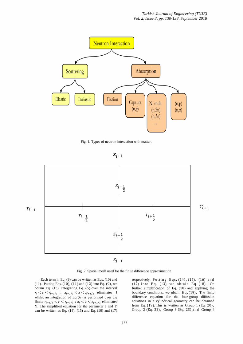
Turkish Journal of Engineering (TUJE)
Vol. 2, Issue 3, pp. 130-138, September 2018
133
Fig. 1. Types of neutron interaction with matter.
Fig. 2. Spatial mesh used for the finite difference approximation.
Each term in Eq. (9) can be written as Eqs. (10) and
(11). Putting Eqs. (10), (11) and (12) into Eq. (9), we
obtain Eq. (13). Integrating Eq. (5) over the interval
𝑟𝑖 < 𝑟 < 𝑟𝑖+1/2 ; 𝑧𝑗−1/2 < 𝑧 < 𝑧𝑗+1/2 eliminates J
whilst an integration of Eq.(6) is performed over the
limits 𝑟𝑖−1/2 < 𝑟 < 𝑟𝑖+1/2 ; 𝑧𝑗 < 𝑧 < 𝑧𝑗+1/2 eliminates
Y. The simplified equation for the parameter J and Y
can be written as Eq. (14), (15) and Eq. (16) and (17)
respectively. P u t t i n g E q s . (14) , (15), (16) a n d
(17) i n to E q . (13), we o b t a i n E q . (18) . On
further simplification of Eq. (18) and applying the
boundary conditions, we obtain E q . (19) . The finite
difference equation for the four-group diffusion
equations in a cylindrical geometry can be obtained
from Eq. (19). This is written as Group 1 (Eq. 20),
Group 2 (Eq. 22) , Group 3 (Eq. 23) a n d Group 4
𝒛𝒋+𝟏
𝑧𝑗−1
𝑟𝑖+1
𝑟𝑖−12
𝑟𝑖−1 𝑟𝑖+1
2
𝑧𝑗−12
𝑧𝑗+12
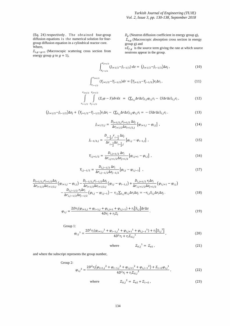
Turkish Journal of Engineering (TUJE)
Vol. 2, Issue 3, pp. 130-138, September 2018
134
(Eq. 24) respectively . Th e o b t a in e d four-group
diffusion equations i s t h e numerical solution for four-
group diffusion equation in a cylindrical reactor core.
Where,
𝛴𝑠,𝑔→𝑔+1 (Macroscopic scattering cross section from
energy group 𝑔 to 𝑔 + 1),
𝐷𝑔 (Neutron diffusion coefficient in energy group g),
𝛴𝑎,𝑔 (Macroscopic absorption cross section in energy
group g) and
𝜐𝛴𝑓,𝑔 is the source term giving the rate at which source
neutrons appear in the group.
∫ (𝐽𝑖+1 2⁄ −𝐽𝑖−1 2⁄ )𝑧𝑗+1 2⁄
𝑧𝑗−1 2⁄
𝑑𝑧 = (𝐽𝑖+1 2⁄ −𝐽𝑖−1 2⁄ )∆𝑧𝑗 , (10)
∫ (𝑌𝑗+1 2⁄ −𝑌𝑗−1 2⁄ )𝑑𝑟𝑟𝑖+1 2⁄
𝑟𝑖−1 2⁄
= (𝑌𝑗+1 2⁄ −𝑌𝑗−1 2⁄ )𝑟𝑖∆𝑟𝑖 , (11)
∫ ∫ (𝛴𝑡𝜑 − 𝑆)𝑑𝑟𝑑𝑧
𝑧𝑗+1 2⁄
𝑧𝑗−1 2⁄
= (∑𝑡𝑖,𝑗∆𝑟∆𝑧)𝑖,𝑗𝜑𝑖,𝑗𝑟𝑖 − (𝑆∆𝑟∆𝑧)𝑖,𝑗𝑟𝑖 ,
𝑟𝑖+1 2⁄
𝑟𝑖−1 2⁄
(12)
(𝐽𝑖+1 2⁄ −𝐽𝑖−1 2⁄ )∆𝑧𝑗 + (𝑌𝑗+1 2⁄ −𝑌𝑗−1 2⁄ )𝑟𝑖∆𝑟𝑖 − (∑𝑡𝑖,𝑗∆𝑟∆𝑧)𝑖,𝑗𝜑𝑖,𝑗𝑟𝑖 = − (𝑆∆𝑟∆𝑧)𝑖,𝑗𝑟𝑖 . (13)
𝐽𝑖+1 2⁄ ,𝑗 = 𝐷𝑖+1/2,𝑗𝑟𝑖+1/2 ∆𝑧𝑗
∆𝑟𝑖+1/2∆𝑧𝑖+1/2,𝑗[𝜑𝑖+1,𝑗 − 𝜑𝑖,𝑗] , (14)
𝐽𝑖−1 2⁄ ,𝑗 =
𝐷𝑖−
12
,𝑗𝑟
𝑖−12
∆𝑧𝑗
∆𝑟𝑖−
12
∆𝑧𝑖−
12
,𝑗
[𝜑𝑖,𝑗 − 𝜑𝑖−1,𝑗] , (15)
𝑌𝑖,𝑗+1 2⁄ = 𝐷𝑖,𝑗+1 2⁄ ∆𝑟𝑖
∆𝑟𝑖,𝑗+1 2⁄ ∆𝑧𝑗+1/2[𝜑𝑖,𝑗+1 − 𝜑𝑖,𝑗] , (16)
𝑌𝑖,𝑗−1 2⁄ = 𝐷𝑖,𝑗−1 2⁄ ∆𝑟𝑖
∆𝑟𝑖,𝑗−1 2⁄ ∆𝑧𝑗−1/2[𝜑𝑖,𝑗 − 𝜑𝑖,𝑗−1] , (17)
𝐷𝑖+1/2,𝑗𝑟𝑖+1/2∆𝑧𝑗
∆𝑟𝑖+1/2∆𝑧𝑖+1/2,𝑗(𝜑𝑖+1,𝑗 − 𝜑𝑖,𝑗) −
𝐷𝑖−1/2,𝑗𝑟𝑖−1/2∆𝑧𝑗
∆𝑟𝑖+1/2∆𝑧𝑖+1/2,𝑗(𝜑𝑖,𝑗 − 𝜑𝑖−1,𝑗) +
𝐷𝑖,𝑗+1 2⁄ 𝑟𝑖∆𝑟𝑖
∆𝑟𝑖,𝑗+1 2⁄ ∆𝑧𝑗+1/2(𝜑𝑖,𝑗+1 − 𝜑𝑖,𝑗)
−𝐷𝑖,𝑗−1 2⁄ 𝑟𝑖∆𝑟𝑖
∆𝑟𝑖,𝑗−1 2⁄ ∆𝑧𝑗−1/2(𝜑𝑖,𝑗 − 𝜑𝑖,𝑗−1) − 𝑟𝑖,𝑗∑𝑡𝑖,𝑗
𝜑𝑖,𝑗∆𝑟𝑖∆𝑧𝑗 = −𝑟𝑖,𝑗𝑆𝑖,𝑗∆𝑟𝑖∆𝑧𝑗 . (18)
𝜑𝑖,𝑗 =2𝐷𝑟𝑖(𝜑𝑖+1,𝑗 + 𝜑𝑖−1,𝑗 + 𝜑𝑖,𝑗+1 + 𝜑𝑖,𝑗−1) + 𝑟𝑖[𝑆𝑖,𝑗]∆𝑟∆𝑧
4𝐷𝑟𝑖 + 𝑟𝑖𝛴𝑡 . (19)
Group 1:
𝜑𝑖,𝑗1 =
2𝐷1𝑟𝑖(𝜑𝑖+1,𝑗1 + 𝜑𝑖−1,𝑗
1 + 𝜑𝑖,𝑗+11 + 𝜑𝑖,𝑗−1
1) + 𝑟𝑖[𝑆𝑖,𝑗1]
4𝐷1𝑟𝑖 + 𝑟𝑖𝛴𝑡𝑖,𝑗1 , (20)
where 𝛴𝑡𝑖,𝑗1 = 𝛴𝑎1 , (21)
and where the subscript represents the group number,
Group 2:
𝜑𝑖,𝑗2 =
2𝐷2𝑟𝑖(𝜑𝑖+1,𝑗2 + 𝜑𝑖−1,𝑗
2 + 𝜑𝑖,𝑗+12 + 𝜑𝑖,𝑗−1
2) + 𝛴1→2𝜑𝑖,𝑗1
4𝐷2𝑟𝑖 + 𝑟𝑖𝛴𝑡𝑖,𝑗2 , (22)
where 𝛴𝑡𝑖,𝑗2 = 𝛴𝑎2 + 𝛴1→2 , (23)

Turkish Journal of Engineering (TUJE)
Vol. 2, Issue 3, pp. 130-138, September 2018
135
Group 3:
𝜑𝑖,𝑗3 =
2𝐷3𝑟𝑖(𝜑𝑖+1,𝑗3 + 𝜑𝑖−1,𝑗
3 + 𝜑𝑖,𝑗+13 + 𝜑𝑖,𝑗−1
3) + 𝛴2→3𝜑𝑖,𝑗2
4𝐷3𝑟𝑖 + 𝑟𝑖𝛴𝑡𝑖,𝑗3 (24)
where 𝛴𝑡𝑖,𝑗3 = 𝛴𝑎3 + 𝛴1→3 + 𝛴2→3 , (25)
Group 4:
𝜑𝑖,𝑗4 =
2𝐷3𝑟𝑖(𝜑𝑖+1,𝑗4 + 𝜑𝑖−1,𝑗
4 + 𝜑𝑖,𝑗+14 + 𝜑𝑖,𝑗−1
4) + 𝛴3→4𝜑𝑖,𝑗3
4𝐷4𝑟𝑖 + 𝑟𝑖𝛴𝑡𝑖,𝑗4 , (26)
where 𝛴𝑡𝑖,𝑗4 = 𝛴𝑎4 + 𝛴1→4 + 𝛴2→4 + 𝛴3→4 . (27)
Next, TUNTOB proceeds from the first group to
the second, third and fourth group, iterating within each
group until the criteria convergence is met. It evaluates
the tolerance between the old and the new 𝒌𝒆𝒇𝒇 values.
To calculate the new 𝒌𝒆𝒇𝒇, the program integrates the
old and new source terms over space and essentially
averages them. With the updated source and 𝒌𝒆𝒇𝒇, the
iterations are performed again. The process continues
until convergence is met. Next the program checks if
the reactor is critical. If 𝒌𝒆𝒇𝒇 is very close to or equal to
one (1), the system is critical. If the reactor is not
critical, the program will again recommend an adjusted
value for the core geometry, guessed multiplication
factor (k) and flux.
3.2. Design of the Algorithm (TUNTOB)
The algorithm was designed using Matlab. Matlab
was used because its algorithms can be developed in
much shorter time than equivalent FORTRAN or
C programs (Kiusalaas, 2005). The TUNTOB
algorithm was developed for the criticality calculations
of a homogenous cylindrical reactor core using four-
group diffusion equations. The flow chart of the
proposed algorithm is shown in Fig. 3.
4. RESULTS AND DISCUSSION
4.1. Iteration and Mesh Sizes Optimization
4.1.1. Iteration optimization
The calculations of the iteration optimization are
shown in Table 1. A maximum of 1000 and a minimum
of 600 iterations were performed. The 1000th iteration
was performed for a 12 cm x 24 cm mesh size of the
reactor core. The Table 1 shows the values of the
effective multiplication factor of the same mesh size
with the number of iterations (600-1000). It was
observed that an increment in iteration leads to an
increase in the effective multiplication factor obtained
from 0.9983 to 0.9990 with a corresponding increase in
the computation time. The maximum effective
multiplication factor of (𝒌𝒆𝒇𝒇 = 0.9990) was reached
when the number of iterations were 1000 and above.
Therefore, it was concluded that the optimal number of
iterations required for this calculation is 1000.
Fig. 3. Flow chart of the proposed algorithm
(TUNTOB).
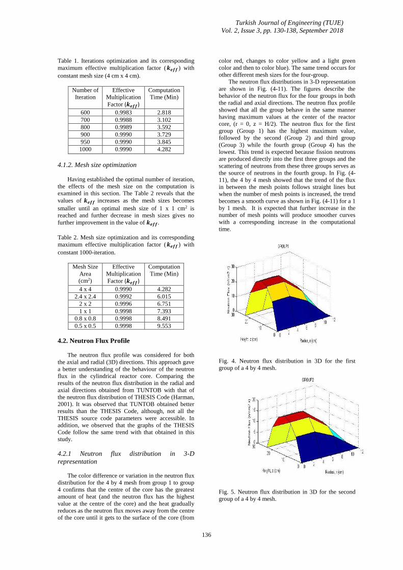
Turkish Journal of Engineering (TUJE)
Vol. 2, Issue 3, pp. 130-138, September 2018
136
Table 1. Iterations optimization and its corresponding
maximum effective multiplication factor (𝒌𝒆𝒇𝒇 ) with
constant mesh size (4 cm x 4 cm).
Number of
Iteration
Effective
Multiplication
Factor (𝒌𝒆𝒇𝒇)
Computation
Time (Min)
600 0.9983 2.818
700 0.9988 3.102
800 0.9989 3.592
900 0.9990 3.729
950 0.9990 3.845
1000 0.9990 4.282
4.1.2. Mesh size optimization
Having established the optimal number of iteration,
the effects of the mesh size on the computation is
examined in this section. The Table 2 reveals that the
values of 𝒌𝒆𝒇𝒇 increases as the mesh sizes becomes
smaller until an optimal mesh size of 1 x 1 cm2 is
reached and further decrease in mesh sizes gives no
further improvement in the value of 𝒌𝒆𝒇𝒇.
Table 2. Mesh size optimization and its corresponding
maximum effective multiplication factor (𝒌𝒆𝒇𝒇 ) with
constant 1000-iteration.
Mesh Size
Area
(cm2)
Effective
Multiplication
Factor (𝒌𝒆𝒇𝒇)
Computation
Time (Min)
4 x 4 0.9990 4.282
2.4 x 2.4 0.9992 6.015
2 x 2 0.9996 6.751
1 x 1 0.9998 7.393
0.8 x 0.8 0.9998 8.491
0.5 x 0.5 0.9998 9.553
4.2. Neutron Flux Profile
The neutron flux profile was considered for both
the axial and radial (3D) directions. This approach gave
a better understanding of the behaviour of the neutron
flux in the cylindrical reactor core. Comparing the
results of the neutron flux distribution in the radial and
axial directions obtained from TUNTOB with that of
the neutron flux distribution of THESIS Code (Harman,
2001). It was observed that TUNTOB obtained better
results than the THESIS Code, although, not all the
THESIS source code parameters were accessible. In
addition, we observed that the graphs of the THESIS
Code follow the same trend with that obtained in this
study.
4.2.1 Neutron flux distribution in 3-D
representation
The color difference or variation in the neutron flux
distribution for the 4 by 4 mesh from group 1 to group
4 confirms that the centre of the core has the greatest
amount of heat (and the neutron flux has the highest
value at the centre of the core) and the heat gradually
reduces as the neutron flux moves away from the centre
of the core until it gets to the surface of the core (from
color red, changes to color yellow and a light green
color and then to color blue). The same trend occurs for
other different mesh sizes for the four-group.
The neutron flux distributions in 3-D representation
are shown in Fig. (4-11). The figures describe the
behavior of the neutron flux for the four groups in both
the radial and axial directions. The neutron flux profile
showed that all the group behave in the same manner
having maximum values at the center of the reactor
core, (r = 0, z = H/2). The neutron flux for the first
group (Group 1) has the highest maximum value,
followed by the second (Group 2) and third group
(Group 3) while the fourth group (Group 4) has the
lowest. This trend is expected because fission neutrons
are produced directly into the first three groups and the
scattering of neutrons from these three groups serves as
the source of neutrons in the fourth group. In Fig. (4-
11), the 4 by 4 mesh showed that the trend of the flux
in between the mesh points follows straight lines but
when the number of mesh points is increased, the trend
becomes a smooth curve as shown in Fig. (4-11) for a 1
by 1 mesh. It is expected that further increase in the
number of mesh points will produce smoother curves
with a corresponding increase in the computational
time.
Fig. 4. Neutron flux distribution in 3D for the first
group of a 4 by 4 mesh.
Fig. 5. Neutron flux distribution in 3D for the second
group of a 4 by 4 mesh.
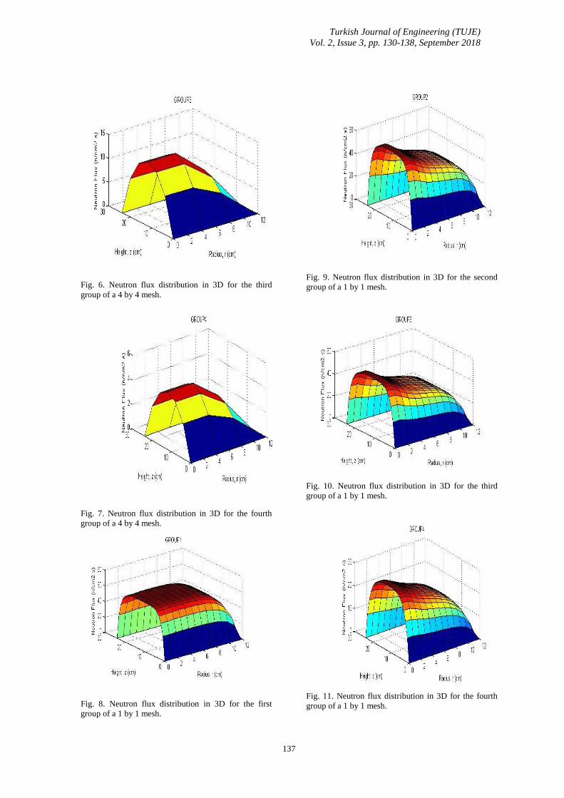
Turkish Journal of Engineering (TUJE)
Vol. 2, Issue 3, pp. 130-138, September 2018
137
Fig. 6. Neutron flux distribution in 3D for the third
group of a 4 by 4 mesh.
Fig. 7. Neutron flux distribution in 3D for the fourth
group of a 4 by 4 mesh.
Fig. 8. Neutron flux distribution in 3D for the first
group of a 1 by 1 mesh.
Fig. 9. Neutron flux distribution in 3D for the second
group of a 1 by 1 mesh.
Fig. 10. Neutron flux distribution in 3D for the third
group of a 1 by 1 mesh.
Fig. 11. Neutron flux distribution in 3D for the fourth
group of a 1 by 1 mesh.

Turkish Journal of Engineering (TUJE)
Vol. 2, Issue 3, pp. 130-138, September 2018
138
In this work, we have derived four group diffusion
equations for a cylindrical reactor core which gives a
detailed description of neutron distribution in the core.
We derived the discretized four group diffusion
equations for a cylindrical reactor core because it gives
an exact description of what takes place in a low water
reactor (LWR). The results obtained for the criticality
calculations were compared with criticality benchmarks
and found to be very close. For instance, the 𝒌𝒆𝒇𝒇
calculated by the code is found to be 1.246728 while
the benchmark value is 1.246368 (Ganapol, 2014).
CONCLUSION
This study provides the criticality calculation and
neutron flux distribution in a homogenous cylindrical
reactor core in two dimensions (r, z) using four energy
groups. From the results these studies further confirm
that the centre of the core of the reactor has the greatest
heat which is synonymous to the different colour
variations relating to decrease in the amount of heat as
it moves away from the centre of the core. The
calculations were carried out for a reactor in a steady
state. The developed algorithm (TUNTOB), calculates
values of 𝒌𝒆𝒇𝒇 and the neutron distribution as a
function of the mesh sizes. It was found that the
accuracy in the value of 𝒌𝒆𝒇𝒇 and the smoothness of the
neutron distribution curves in 3-D representations,
depends on the number of mesh points. It allows the
user to modify the reactor dimensions and see the
impacts on the neutron distribution and criticality
within the reactor core.
ACKNOWLEDGEMENT
Authors wish to acknowledge the support provided
by the Department of Physics and Engineering Physics,
the Center for Energy Research and Development, and
the Department of Electronic and Electrical
Engineering, Obafemi Awolowo University, Ile-Ife,
Nigeria.
REFERENCE
Atomic Energy Control Board of Canada,
Fundamental of Power Reactors. Canada: Atomic
Energy Control Board of Canada (AECBC), pp.
1-3, 1993. Available [online]:
http://www.thecanadianencyclopedia.ca/en/article
/atomic-energy-control-board/
A. Arzhanov, Analytical Models of Critical
Reactor in Simple Geometries, Royal Institute of
Technology, Department of Physics. Stockholm,
Sweden: KTH Engineering Sciences, pp. 1-33,
2010.
B. Ganapol, Verification of the CENTRM Module
for Adaptation of the SCALE Code to NGNP
Prismatic and PBR Core Designs, Univeristy of
Arizona. Arizona: Reactor Concepts RD and D,
2014.
D. B. Ganapol, The Analytical Solution to the
Multigroup Diffusion Equation in One -
Dimensional Plane, Cylindrical and Spherical
Geometries, Joint International Tropical on
Mathematics and Computation and
Supercomputing in Nuclear Application, 2007.
J. D. Burnham, Reactor Theory - The Steady
State, Nuclear Training Course, 1967.
J. J. Duderstadt and J. L. Hamilton, Nuclear
Reactor Analysis. Michigan: John Wiley and
Sons, Inc, 672p, 1976.
J. T. Urbatsch, Iterative Acceleration Methods for
Monte Carlo and Deterministic Criticality.
California: Los Alamos National Laboratory, pp.
1-174, 1995. Available [online]:
https://www.osti.gov/scitech/servlets/purl/212566
J. Kiusalaas, Numerical Methods in Engineering
with Matlab, New York: Cambridge University
Press, pp. 1-435, 2005.
M. A. Jayeola, M. K. Fasasi, A. A. Amosun, A. O.
Salau, B. M. Ojo (2018), Numerical Computation
of Fission-Product Poisoning Build-up and Burn-
up Rate in a Finite Cylindrical Nuclear Reactor
Core, Bilge International Journal of Science and
Technology Research, Vol. 2(1), pp. 17-30.
M. S. Stacey, Nuclear Reactor Physics. Atlanta:
Wiley-Vch Verlag Gmbh and Co. KGaA,
Weinheim, 735p, 2007.
R. J. Larmash and J. A. Baratta, Introduction to
Nuclear Engineering (3rd edition), New Jersey,
420p, 2001.
T. Tanbay and O. Bilge, Numerical Solution of
the Multigroup Neutron Diffusion Equation by
the Meshless RBF Collocation Method,
Mathematical and Computational Applications,
Vol. 18, pp. 399-407, 2013.
W. H. Harman, Modelling Pressurized Water
Reactor Kinetics, Ohio, Wright-Patterson Air
Force Base, 2001.
Copyright © Turkish Journal of Engineering
(TUJE). All rights reserved, including the making
of copies unless permission is obtained from the
copyright proprietors.

VOLUME 2 ISSUE 3 SEPTEMBER 2018
ISSN 2587-1366
CONTENTS
RHEOLOGICAL PARAMETER ESTIMATION OF CMC-WATER
SOLUTIONS USING MAGNETIC RESONANCE IMAGING (MRI)
G. Bengusu Tezel ................................................................................................... 94
INVESTIGATION OF Ni-Mn BASED SHAPE MEMORY ALLOY
VARIATIONS TRANSFORMATION TEMPERATURES
Ece Kalay, Anıl Erdağ Nomer and Mehmet Ali Kurgun ................................... 98
INVESTIGATION OF DISSOLUTION KINETICS OF Zn AND Mn FROM
SPENT ZINC-CARBON BATTERIES IN SULPHURIC ACID SOLUTION
Tevfik Agacayak and Ali Aras ........................................................................... 107
COMPARATIVE STUDY OF REGIONAL CRASH DATA IN TURKEY
Murat Özen.......................................................................................................... 113
PERFORMANCE COMPARISON OF ANFIS, ANN, SVR, CART AND MLR
TECHNIQUES FOR GEOMETRY OPTIMIZATION OF CARBON
NANOTUBES USING CASTEP
Mehmet Acı, Çiğdem İnan Acı and Mutlu Avcı ................................................ 119
INVESTIGATION OF ULEXITE USAGE IN AUTOMOTIVE BRAKE
FRICTION MATERIALS
Banu Sugözü ........................................................................................................ 125
CRITICALITY CALCULATION OF A HOMOGENOUS CYLINDRICAL
NUCLEAR REACTOR CORE USING FOUR-GROUP DIFFUSION
EQUATIONS
Babatunde Michael Ojo, Musibau Keulere Fasasi, Ayodeji Olalekan Salau,
Stephen Friday Olukotun and Ademola Mathew Jayeola................................ 130