volume 7, issue 2 2017sdiwc.net/ijdiwc/files/ijdiwc-print-72.pdf · conference is an easy task....
TRANSCRIPT

ISSN 2225-658X (ONLINE)
ISSN 2412-6551 (PRINT)
Volume 7, Issue 2
2017

International Journal of
DIGITAL INFORMATION AND WIRELESS COMMUNICATIONS
Editor-in-Chief
Dr. Rohaya Latip, University Putra Malaysia, Malaysia
Editorial Board
Abbas M. Al-Ghaili, Universiti Putra Malaysia, Malaysia Ali Sher, American University of Ras Al Khaimah, UAE Altaf Mukati, Bahria University, Pakistan Andre Leon S. Gradvohl, State University of Campinas, Brazil Azizah Abd Manaf, Universiti Teknologi Malaysia, Malaysia Bestoun Ahmed, University Sains Malaysia, Malaysia Carl Latino, Oklahoma State University, USA Dariusz Jacek Jakóbczak, Technical University of Koszalin, Poland Duc T. Pham, University of Bermingham, UK E.George Dharma Prakash Raj, Bharathidasan University, India Elboukhari Mohamed, University Mohamed First, Morocco Eric Atwell, University of Leeds, United Kingdom Eyas El-Qawasmeh, King Saud University, Saudi Arabia
Ezendu Ariwa, London Metropolitan University, United Kingdom Fouzi Harrag, UFAS University, Algeria Genge Bela, University of Targu Mures, Romania Guo Bin, Institute Telecom & Management SudParis, France Hadj Hamma Tadjine, Technical university of Clausthal, Germany Hassan Moradi, Qualcomm Inc., USA Isamu Shioya, Hosei University, Japan Jacek Stando, Lodz University of Technology, Poland Jan Platos, VSB-Technical University of Ostrava, Czech Republic Jose Filho, University of Grenoble, France Juan Martinez, Gran Mariscal de Ayacucho University, Venezuela Kaikai Xu, University of Electronic Science and Technology of China, China Khaled A. Mahdi, Kuwait University, Kuwait Ladislav Burita, University of Defence, Czech Republic Maitham Safar, Kuwait University, Kuwait Majid Haghparast, Islamic Azad University, Shahre-Rey Branch, Iran Martin J. Dudziak, Stratford University, USA Mirel Cosulschi, University of Craiova, Romania Mohamed Amine Ferrag, Guelma University, Algeria Monica Vladoiu, PG University of Ploiesti, Romania Nan Zhang, George Washington University, USA Noraziah Ahmad, Universiti Malaysia Pahang, Malaysia Pasquale De Meo, University of Applied Sciences of Porto, Italy Paulino Leite da Silva, ISCAP-IPP University, Portugal Piet Kommers, University of Twente, The Netherlands Radhamani Govindaraju, Damodaran College of Science, India Ramadan Elaiess, University of Benghazi, Libya Rasheed Al-Zharni, King Saud University, Saudi Arabia Su Wu-Chen, Kaohsiung Chang Gung Memorial Hospital, Taiwan Talib Mohammad, University of Botswana, Botswana Tutut Herawan, University Malaysia Pahang, Malaysia Velayutham Pavanasam, Adhiparasakthi Engineering College, India Viacheslav Wolfengagen, JurInfoR-MSU Institute, Russia Wen-Tsai Sung, National Chin-Yi University of Technology, Taiwan Wojciech Zabierowski, Technical University of Lodz, Poland Yasin Kabalci, Nigde University, Turkey Yoshiro Imai, Kagawa University, Japan Zanifa Omary, Dublin Institute of Technology, Ireland Zuqing Zhu, University of Science and Technology of China, China
Overview The SDIWC International Journal of Digital Information and Wireless Communications is a refereed online journal designed to address the networking community from both academia and industry, to discuss recent advances in the broad and quickly-evolving fields of computer and communication networks, technology futures, national policies and standards and to highlight key issues, identify trends, and develop visions for the digital information domain.
In the field of Wireless communications; the topics include: Antenna systems and design, Channel Modeling and Propagation, Coding for Wireless Systems, Multiuser and Multiple Access Schemes, Optical Wireless Communications, Resource Allocation over Wireless Networks, Security, Authentication and Cryptography for Wireless Networks, Signal Processing Techniques and Tools, Software and Cognitive Radio, Wireless Traffic and Routing Ad-hoc networks, and Wireless system architectures and applications. As one of the most important aims of this journal is to increase the usage and impact of knowledge as well as increasing the visibility and ease of use of scientific materials, IJDIWC does NOT CHARGE authors for any publication fee for online publishing of their materials in the journal and does NOT CHARGE readers or their institutions for accessing to the published materials.
Publisher
The Society of Digital Information and Wireless Communications 20/F, Tower 5, China Hong Kong City, 33 Canton Road, Tsim Sha Tsui, Kowloon, Hong Kong
Further Information Website: http://sdiwc.net/ijdiwc, Email: [email protected], Tel.: (202)-657-4603 - Inside USA; 001(202)-657-4603 - Outside USA.
Permissions International Journal of Digital Information and Wireless Communications (IJDIWC) is an open access journal which means that all content is freely available without charge to the user or his/her institution. Users are allowed to read, download, copy, distribute, print, search, or link to the full texts of the articles in this journal without asking prior permission from the publisher or the author. This is in accordance with the BOAI definition of open access.
Disclaimer Statements of fact and opinion in the articles in the International Journal of Digital Information and Wireless Communications (IJDIWC) are those of the respective authors and contributors and not of the International Journal of Digital Information and Wireless Communications (IJDIWC) or The Society of Digital Information and Wireless Communications (SDIWC). Neither The Society of Digital Information and Wireless Communications nor International Journal of Digital Information and Wireless Communications (IJDIWC) make any representation, express or implied, in respect of the accuracy of the material in this journal and cannot accept any legal responsibility or liability as to the errors or omissions that may be made. The reader should make his/her own evaluation as to the appropriateness or otherwise of any experimental technique described.
Copyright © 2017 sdiwc.net, All Rights Reserved
The issue date is June 2017.

IJDIWC
ISSN 2225-658X (Online) ISSN 2412-6551 (Print)
Volume 7, Issue No. 2 2017
TABLE OF CONTENTS
PAPER TITLE AUTHORS PAGES
A PROTOTYPE OF ADVANCED MANAGEMENT INFORMATION SYSTEM FOR CONFERENCES
Kota Morigaki, Keizo Saisho 60
DYNAMIC OPTIMIZATION OF IEEE 802.11 DCF BASED ON ACTIVE STATIONS AND COLLISION PROBABILITY
Nithya Balasubramanian, Shreenivas Bharadwaj Venkataramanan and Aravind Aathma
66
Modeling Improved Low Latency Queueing Scheduling Scheme for Mobile Ad Hoc Networks
Kakuba Samuel, Kyanda S. Kaawaase, Michael Okopa
75
Mining Top-T Web Traversal Subsequences Santosh Kumar, Neha Tyagi 93
Development of Electronic Document Archive Management System (EDAMS): A Case Study of a University Registrar in the Philippines
Las Johansen B. Caluza 106
Data Mining and Analysis for off Grid Solar PV Power System
Mohamed D. Almadhoun 118
Vulnerability Assessment and Penetration Testing: A proactive approach towards Network and Information Security
Muhammad Zeeshan, Shams Un Nisa, Tazeen Majeed, Nayab Nasir, Saadia Anayat
124

A Prototype of Advanced Management Information System for Conferences
George Kastanian and Eyas El-Qawasmeh
University of Nizwa, Oman
[email protected] and [email protected]
ABSTRACT
This paper aims to describe the experience
accumulated in building a sophisticated management
information system for conferences. The accumulated
experience is built over 6 years and it is implemented
in real life where six editions of the same conference
were conducted over six countries. After that, the
authors suggested a framework for a successful
management system that keeps track of all data and
processing emails in an efficient and accurate way.
The implementation of such framework results in
reducing the work time and gives more accurate
information to the researchers.
Keywords Conferences, reviewing, publications
1 INTRODUCTION
As we know, conferences represent an important
atmosphere to bring people all over the world
together in one place where they can discover
and share the same passion and interests. In
addition, it gives opportunities to the researchers
to exchange ideas, research and establish further
communications [2] [3].
Many people think that conducting a scientific
conference is an easy task. However, running a
conference is incredibly hard, much more than
you can possibly imagine. Statistics showed that
on average for every 1000 visitors for any
conference website, only one of them is
interested. Thus, attracting the attention of
people is a hard task and the most effective
factor of the success of any conference[4] [5].
The statistics are confirmed from the cookies
that some conferences added to get statistics. See
Figure 1.
Figure 1. No. of visitors using statcounter code added to a
conference website
Running a conference requires to work smarter
(and not harder) several months before it for
preparations through conference management
system which is an online application that will
help to take care of the details such as: sending
invitations to attract scientific research papers,
reviewing, notifications, finalize the procedure
like submitting final camera ready and
copyrights, collecting registration, preparing the
proceedings which will contain the final papers
that will be published, and finally evaluating the
success of the conference.
To run a successful conference, many factors
must exist. These factors must be plugged into
the conference management system. In addition,
some factors must be avoided. A detailed
description of such factors is listed later with
more details.
The organization of this paper as follows:
Section 2 describes the environment of
conferences. Section 3 describes the tools for
any conference management system. Section 4
describes the integration of a conference

management system with different components.
The section 5 is the performance results and
section 6 discussion and section 7 is a
conclusion.
2 THE ENVIRONMENT OF
CONFERENCES
With the spread of the internet and the spread of
the social media, several challenges appear for
conducting any scientific conference. The
challenges include:
1. Funding and Budget
2. High competition. This is resented by the
publicity process which should reach
right persons and the fact of the existence
of hundreds of conferences yearly in the
same scope.
To overcome these challenges, the following
factors must exist in order to cope with the
rapidly changing environment. This includes:
1. Be organized and allocate tasks to the
committee and the managers of the
conference.
2. Response time must be fast to deal with
the problems from the possible attendees
with registration or transportation or visa
issues as soon as possible.
3. Quality of the research. For example,
checking for Plagiarism.
4. Good tracking system for reviewing.
5. Good indexing after publications.
6. Selecting high quality journals for the
best selected papers of the conference.
7. Approach transportation and
accommodation facilities for possible
special conference rates.
In addition, the conference management system
must avoid factors that degrade its performance
[6] [7] [8]. These include: 1) Phishing by
sending some fake papers, and 2) Not serious
reviewers.
3 TOOLS FOR ANY INFORMATION
SYSTEMS
In this section, we are going to describe the tools
for any successful conference management
system. These include:
1. Smart sheet: This enables managers to
automate the collaborative work of the
conference managers within a platform
trusted by the world‟s most productive
companies. The platform provides with
an area to assign tasks to all the managers
who handle all the tasks of the
conference.
Figure 2. Smart sheet template
2. Automation of paper submission by using
the conference management system.
Therefore, authors will be able to submit
their research papers online without the
help of the workers who work on the
conference [1]. Figure 3 gives an
example of this.
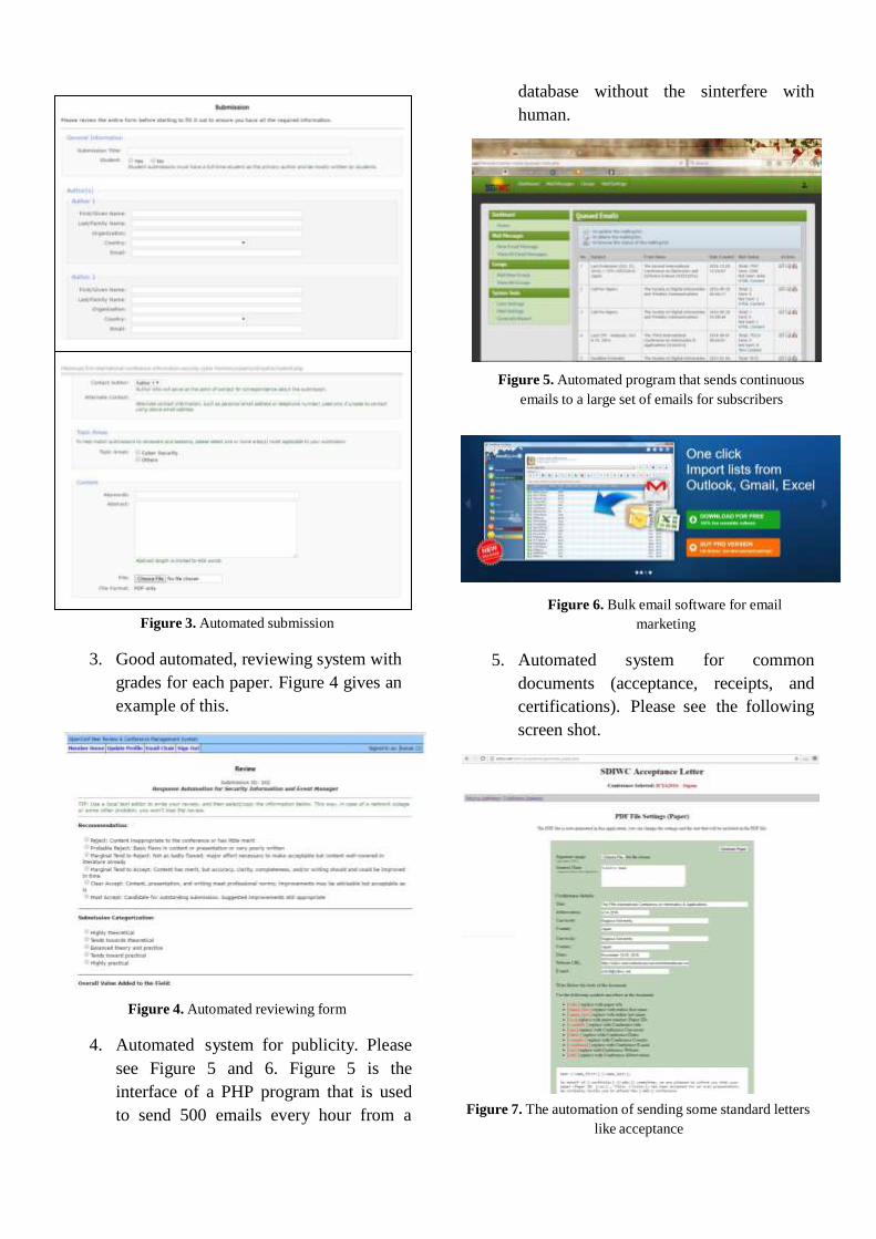
database without the sinterfere with
human.
Figure 5. Automated program that sends continuous
emails to a large set of emails for subscribers
Figure 3. Automated submission
3. Good automated, reviewing system with
grades for each paper. Figure 4 gives an
example of this.
Figure 4. Automated reviewing form
4. Automated system for publicity. Please
see Figure 5 and 6. Figure 5 is the
interface of a PHP program that is used
to send 500 emails every hour from a
Figure 6. Bulk email software for email
marketing
5. Automated system for common
documents (acceptance, receipts, and
certifications). Please see the following
screen shot.
Figure 7. The automation of sending some standard letters
like acceptance

6. Online registration, which saves the time
and ensures a secure, reliable registration
process for the attendee/participant.
Figure 8. Online Registration
7. Automated conference schedule. Figure 9
shows the example.
Figure 9. Automated conference program
4 INTEGRATION OF INFORMATION
SYSTEM COMPONENTS
The Figure 10 shows the overall framework for
the system that integrated with the database and
the staff.
Figure 10. Overall system intergrade with the database
and the staff.
5 PERFORMANCE RESULTS
The existing prototype listed in Figure 10 saves
time. The reason is that it sends personalized
email, but it goes as bulky and one shot.
Following is one figure.
Figure 11. Bulky emails go personalized where you can
send any number of emails in one shot.

This save in time also comes from other sources
such as sending acceptance automatically.
The second contribution is the accuracy of
recording the grades for the reviewing of each
paper. The reviewing is recorded accurately as
you can see in the following figure.
(b)
Figure 12. Sample Grade and Reviewing [1]
6 DISCUSSION
Any conference suffers from problems that
cannot be solved easily. The reason is that the
control of these problems is outside the
management of any conference [5]. Among these
problems and their suggested solution in this
paper are:
- Delay in doing the tasks. It is observed
that most researchers submit their papers
in the last week of the submission date.
This creates unbalanced load on the
reviewing process and on the work. The
solution is that the management must be
ready for last minute submission by
processing tasks upon their arrival.
(a)
- Reviewers who are not serious. Those
reviewers are late in submitting their
reviewing or they did not read the paper
carefully (in particular third world
reviewers). Examples of these are in the
Figure 13. The solution is to discard
these reviewing.

7 CONCLUSION
Figure 13. Unserious reviews
The presented framework was implemented
successfully in DICTAP conference, which has
been conducted until today in 6 countries. The
framework proved its efficiency and
effectiveness due to the high number of
registered papers in this conference. The
accumulated experience with the suggested
framework can be further implemented in just
one big system.
REFERENCES
1. Open conference website.
2. The Keynote Guide to Planning a Successful
Conference by Cathy Key.
3. Wolfgang Reinhardt, Martin EbnerΓ, Günter Beham,
Cristina Costa “How People are using Twitter during
Conferences”, Creativity and Innovation
Competencies on the Web, Hornung-Prähauser, V.,
Luckmann, M. (Ed.) Proceeding of 5. Edu Media
conference, p. 145-156, Salzburg.
4 Charlotte N. Gunawardena, “Social Presence
Theory and Implications for Interaction and
Collaborative Learning in Computer
Conferences”, International Jl. of Educational
Telecommunications (1995) 1(2/3), 147-166.
5 Manos Papagelis, Dimitris Plexousakis,
Panagiotis N. Nikolaou. “CONFIOUS: Managing
the Electronic Submission and Reviewing Process
of Scientific Conferences (2005), p. 1
6 Ralph Grishman, Beth Sundheim, Message
Understanding Conference - 6: A Brief History”
p. 466-471.
7 A Framework for Conference Control Functions,
by Nadia Kausar. A Ph.D thesis.
8 Bharat Gupta, O.P.Gupta, B.K. Sawhney, "A
Framework for Conference Management
System"(2014).

Dynamic Optimization of IEEE 802.11 DCF based on Active Stations and Collision
Probability
Nithya Balasubramanian, Shreenivas Bharadwaj Venkataramanan and Aravind Aathma
Department of Computer Science and Engineering
National Institute of Technology,
Tiruchirapalli-620015, Tamil Nadu, India
{bnithyanitt, vshreenivasbharadwaj, aravind.cps}@gmail.com
ABSTRACT
In IEEE 802.11 wireless networks, the back-off
algorithm has an exponential Contention Window
(CW) increment and resetting CW strategy. Under
heavy network load conditions the traditional Binary
Exponential Back-off (BEB) algorithm has very low
throughput and high collision probability. In this
paper, an algorithm called Dynamically Optimized
Contention Window (DOCW) is introduced to
estimate the optimal Contention Window CWopt
according to the number of active competing stations
and the current collision probability. The proposed
algorithm dynamically adapts CW with respect to the
current network states. Simulation of the proposed
DOCW algorithm has been conducted to measure
various parameters like throughput, collision
probability, control overhead and packet loss. The
simulation results for varying number of station
reveal that the proposed algorithm outperforms the
existing Novel Contention Window Back-off
(NCWB) and the traditional BEB in randomly
formed topologies.
KEYWORDS
DCF, Contention Window, Collision Probability,
Wireless Networks, Heuristic, Regression.
1 INTRODUCTION
IEEE 802.11 wireless networks utilize the
Distributed Coordination Function (DCF) to
capture the shared medium with minimum of
collisions. DCF follows the Carrier Sense
Multiple Access with Collision Avoidance
(CSMA/CA) protocol with Binary Exponential
Back-off algorithm (BEB). In this mechanism,
when a station is ready to transmit a packet, it
senses the channel for an idle period equal to one
Distributed Inter Frame Space (DIFS) [1]. If the
channel remains unoccupied, the station
transmits packet, otherwise, the transmission is
paused until the current transmitting event is
terminated. The stations continue to sense the
channel until the medium is idle for DIFS
interval, then a random back-off interval is
generated. Random back-off intervals are
discrete and hence slotted that is the packets are
transmitted only at the beginning of each time
slot. The random back-off value is chosen from
the range [0, CWcurrent − 1] with all values having
equal probability of selection.
Whenever there is a collision between two or
more stations as they transmit their packets, CW
size is doubled. The back-off counter is
suspended when detecting busy medium, and
resumed after sensing an idle medium for the
duration of DIFS interval. The back-off counter
starts decrementing and continues to decrease as
long as the idle medium is sensed. When the
back-off timer reaches zero, the station transmits
a packet at the beginning of the next time slot.
On receiving the packet successfully, the
receiver waits for duration of Short Inter Frame
Space (SIFS) and transmits an Acknowledgment
(ACK) packet. On the other hand, if the
transmission is unsuccessful which is interpreted
by a timeout event in transmitter, a
retransmission of the packet is scheduled and the
CWcurrent is doubled with each unsuccessful
transmission until it reaches its maximum value,
i.e., CWmax = 2m x CWmin, where m indicates
maximum number of retransmissions. After
reaching the maximum limit, the pending packet
may be dropped or handled appropriately based
on different implementations.
The major dependence on BEB drastically limits
the performance of IEEE 802.11 wireless
networks [2]. Large available bandwidth is not
efficiently utilized in a high traffic and a
congested network which results in the
extremely poor performance of BEB [3]. Several

backoff algorithms have been proposed to amend
the efficiency of BEB such as the Exponential
Increase Exponential Decrease (EIED)[4],
Multiplicative Increase Linear Decrease
(MILD)[5], Linear Increase Linear Decrease
(LILD)][5], Smart Exponential Threshold Linear
(SETL)[6], etc. which modified CW size either
linearly or exponentially by various methods
described later in Section 2. The problem with
all these algorithms is that they cannot handle
drastic variations of the network states and
decrease the CW in a similar fashion on
successful transmission. Apart from the heavy
network load, collisions can also occur when two
stations sharing the same channel have equal
back-off counter value [7]. It clearly states the
need for a back-off algorithm which is
Section 2 discusses the related backoff
algorithms with their CW adjusting strategies
and highlights their limitations. In Section 3, the
proposed algorithm is presented along with a fast
efficient implementation for calculating CW opt.
Section 4 presents the simulation results
acquired from NS2 simulation and analyzes the
performance of the proposed DOCW algorithm
with other algorithms. Finally, the section 5
gives the concluding statements.
2 RELATED WORKS
2.1 EIED
This algorithm is based on exponential
increment and decrements of CW.
dynamically optimized based on the network
state. Algorithms like NCWB which overcomes cwi
min(r1.cwi 1 , cwmax ) , on collision
cwi1
the above limitations have a drawback that it does not consider the factor of collision
cwi
max rD
, cwmin ,
on success
probability in computing CW [8].
In this paper, a new Contention Window back-
off algorithm called Dynamically Optimized
Contention Window Back-off (DOCW) is
proposed. This algorithm utilizes two decision
parameters such as the number of active
contending stations [9][10] and the current
collision probability derived from Bianchi‟s
Markov model. The current collision probability
factor gives extra acute information about the
traffic of the network [11], thus improving the
efficiency and if not included in the calculation,
contention window may frequently deviate by a significant amount from the ideal contention
where r1 and rD are respectively the tweaking
factors of the algorithm which can be optimized
differently based on varying network conditions.
The drawback of this algorithm is that it does not
utilize the entire network bandwidth on high
network loads. The CW becomes larger than
desired and smaller than required, causing
unnecessary delays.
2.2 MILD
Multiplicative increment and linear decrements
of CW is proposed and which is given as
follows:
window. The collision probability factor cwi min (1.5.cw i1 , cw max ), on collision
provides an inconceivable boundary to the cwi max( cwi1 1, cwmin ), on success
contention window keeping it from getting out of bounds. The collision probability can also
enhance quality of service (QOS) considerably
[12].The CW opt is increased when number of
active stations in the network increase and
similarly reduce the CW opt when number of
active competing stations decrease. The DOCW
performs significantly better under heavy
network load conditions.
In this paper an efficient method to implement
Though the algorithm slightly performs better
than EIED, similar drawbacks such as the
inefficient use of the total network bandwidth
and usage of non-optimal CW is still prevalent.
2.3 LILD
This algorithm for the modification of CW is
based on linear increment and linear decrement
as shown below,
the algorithm and the environment of simulation
is also presented. The simulation results for the
cwi
cwi
min(cwi1 cwmin , cwmax ) ,
max( cwi1 cwmax , cwmin ) ,
on collision
on success traditional BEB, NCWB and the proposed algorithm DOCW are presented. The rest of the
sections in the paper is structured as follows:
The linear increment and decrement does not
accurately imitate the network load pattern and

3 3
3
thus cannot be used for an efficient utilization of
the network bandwidth.
by the (m, k) form and the method defined as
follows:
2.4 SETL cw
new 2
V D . cwcurrent , no. of transmissions k
This algorithm is a novel combination of EIED and LILD. It defines a threshold value of
cwnew . cwcurrent , no. of transmissions k
CWthreshold and when the CWcurrent exceeds the
threshold then it is tuned down in a clever
manner. Though this algorithm is better than its
predecessors it still does not adapt itself
accordingly to the network state and thus can
still be improved.
2.5 NCWB
This novel algorithm considers the number of
This algorithm does not adapt itself to the
current network state and does not consider the
influence of collision probability on the CW.
2.8 Priority based
The priority based method [13] seeks to solve
the congestion problem by assigning priority
weights to each node based on the traffic pattern.
competing stations to compute the CW as shown
below,
0 to
cwmax
3
1 ,
if priority 1 n.cwmin cwopt min , cwmax ,
2
on collision cw cw max to 2cwmax 1,
if priority 2
i n.cw cw max min , cw , on success 2.cwmax
opt
2 min
to cwmax 1,
if priority 3
where n is the number of active contending stations. The major drawback in this algorithm is
that it does not consider collision probability in
CW calculation.
2.6 LMILD
The algorithm Linear/Multiplicative Increase
Linear Decrease provides a way to handle the
excess traffic in the network. The factor mc, lc
and ls provide a tweaking and optimizing
opportunity. It can adapt the network to different
conditions.
Priority based method is a manual approach to
tackle the congestion problem and can become
very tedious. It does not consider the current
traffic pattern and collision probability in the
computation of CW.
All the above algorithms suffer from the
disadvantage that they either modify CW
linearly or exponentially or cannot handle drastic
variations of the network states. They decrease
CW in a similar fashion on successful
transmission and also not considering collision
probability factor in the CW. Apart from that, in cw min (m
c .cw , cw
max ) ,
cw min(cw l
c , cw
max ) ,
cw min(cw ls , cw
min ) ,
on collision
overheard collision
on success
heavy network load, collisions can also occur
when two stations sharing the same channel may
have equal back-off counter. The collision
The drawback is that though it provides an
opportunity to adapt the algorithm it has to be
done manually by tweaking the parameters.
Manual optimization can be tedious and time
consuming. It does not consider the collision
probability in the CW computation thus losing
vital information of the network.
2.7 MKBS
(m, k) back-off scheme uses the (m, k) form to
determine the value of CW. VDβ is determined
probability keeps the CW in check by providing a numerical restraint preventing it from going
out of bounds. It also supplies the algorithm with
vital information about traffic of the network
improving efficiency of the algorithm and
stabilizing it by not allowing it to fluctuate
much.
The objective and motivation of the proposed
DOCW algorithm is to handle all these
drawbacks, include collision probability factor
and the network state in CW computation and
come up with a better algorithm.

3 PROPOSED DOCW ALGORITHM
The proposed DOCW algorithm makes use of
the number of active stations computed from the
Markov chain model, the current collision
probability. It updates CW size appropriately
thus resulting in an algorithm which efficiently
adapts itself accordingly to the current network
state and load.
Figure 1. State Transitions for the Proposed Algorithm
The number of active stations and the current
collision probability is calculated in the state
module in the lower part of the diagram and both
the parameters (pc, n) are sent to all other
modules for further computations. The collision
state is invoked whenever there is a collision and
success state is invoked on a success. There is
also an initial state with CW value of 32 from
which the success and collision states can be
reached depending on whether success or failure.
There are self-loops in collision and success
states indicating the possibility of multiple
successes or collisions. Similarly the success and
collision states can directly interchange between
themselves depending on whether success or
failure. The collision and success modules are
defined later in the paper.
3.1 Markov Chain model
The number of active stations and collision
probability are computed from the model
proposed by Bianchi [14]. Saturation condition is
assumed in this model that is all stations always
have ready packets for transmission. Each packet
waits for a random back-off time prior to its
transmission. For a given station, let c(t) be the
stochastic process constituting it‟s back-off time
counter. Note that t is discrete and slotted. The
back-off time counter of each station decrements
at the beginning of each slot time which is
unrelated to real time. The back-off timer
decrements are halted when detecting busy
medium. The time interval between beginnings
of two consecutive slots may be longer than the
slot time of constant size T, as it may also
include a packet transmission. Value of the back-
off counter c(t) of each station depends on its
transmission history and thereby violating the
Markov property.
Figure 2. Markov Chain model
We define cw = CWmin and m be the maximum
back-off stage, such that CWmax = 2m.cw, and let
cwi = 2i.cw, where i ϵ (0, m). Let CW(t) be the
stochastic process which is used to represent the
back-off stage (0 → m) of the station at time t.
The key approximation based on the Markov
chain model is that, at each transmission attempt,
all packets collide with constant and independent
probability pc irrespective of the number of
retransmissions incurred. The Markov chain
process is represented by {c(t), CW(t)} as shown
in Figure 2 [14]. In this Markov chain model, the
non-null one-step transition probabilities are:
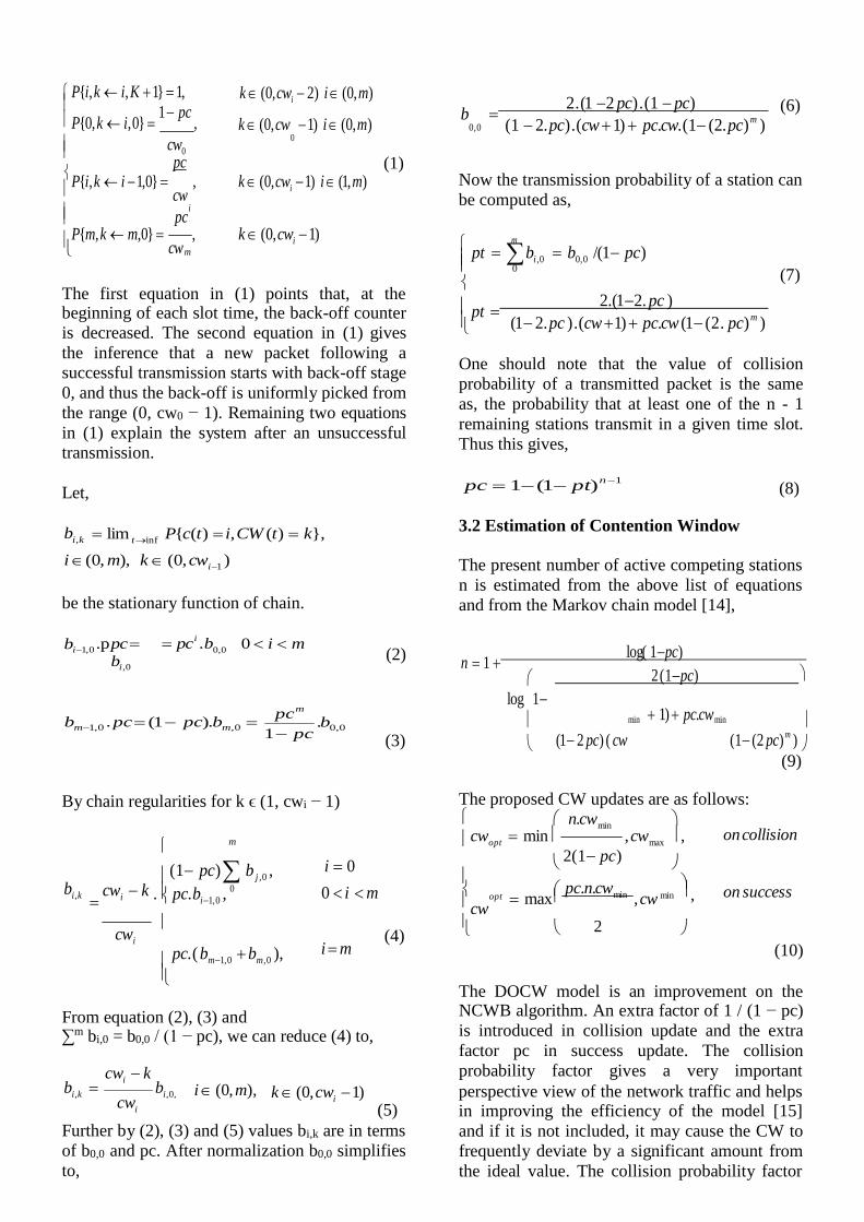
0,0
,
P{i,k i, K 1} 1,
k (0,cwi 2) i (0,m)
b 2. (1 2 pc) . (1 pc)
(6) P{0,k i,0}
1pc ,
k (0,cw
1) i (0,m)
0,0
(1 2.pc).(cw 1) pc.cw.(1(2.pc)m
) cw0
pc
0
(1)
P{i,k i 1,0}
cw , k (0,cwi 1) i (1,m) Now the transmission probability of a station can
i
pc be computed as,
P{m,k m,0} cw
, k (0,cwi 1) m
m pt bi ,0 b0,0 /(1pc) 0
(7) The first equation in (1) points that, at the beginning of each slot time, the back-off counter
is decreased. The second equation in (1) gives
the inference that a new packet following a
successful transmission starts with back-off stage
0, and thus the back-off is uniformly picked from
the range (0, cw0 − 1). Remaining two equations
in (1) explain the system after an unsuccessful
transmission.
pt 2.(12. pc )
(12. pc ).(cw 1) pc.cw (1(2. pc)m
)
One should note that the value of collision
probability of a transmitted packet is the same
as, the probability that at least one of the n - 1
remaining stations transmit in a given time slot.
Thus this gives,
Let,
b
i,k
lim t inf
P{c(t) i, CW (t) k},
pc 1(1pt)n 1
3.2 Estimation of Contention Window
(8)
i (0, m), k (0, cwi1
)
The present number of active competing stations
n is estimated from the above list of equations be the stationary function of chain. and from the Markov chain model [14],
bi1,0 .p pc
bi,0
pci .b 0 i m
(2) n 1
log( 1pc)
log 1
2 (1pc)
bm1,0 . pc (1 pc).bm,0 pc
m
1 pc .b0,0
(3)
(12 pc) ( cw
min 1) pc.cw min (1(2 pc)
m )
(9)
By chain regularities for k ϵ (1, cwi − 1) The proposed CW updates are as follows: n.cw
min
m cwopt
min , cwmax
,
2(1pc)
on collision
bi,k
cwi k
(1pc) b j ,0 ,
0 . pc.bi1,0 ,
i 0
0 i m cw
opt
maxpc.n.cw
min , cw
min
on success
cwi
pc.( bm1,0 bm,0 ),
i m (4) 2
(10)
From equation (2), (3) and ∑m bi,0 = b0,0 / (1 − pc), we can reduce (4) to,
cw
i k
The DOCW model is an improvement on the NCWB algorithm. An extra factor of 1 / (1 − pc)
is introduced in collision update and the extra
factor pc in success update. The collision
probability factor gives a very important b
i,k
cwi
bi,0, i (0, m), k (0, cw
i 1)
(5) perspective view of the network traffic and helps in improving the efficiency of the model [15]
Further by (2), (3) and (5) values bi,k are in terms
of b0,0 and pc. After normalization b0,0 simplifies to,
and if it is not included, it may cause the CW to
frequently deviate by a significant amount from
the ideal value. The collision probability factor

provides a restraining effect on the CW and thus
avoids the larger deviations of the CW from the
ideal value.
The collision probability pc is directly
proportional to the optimal Contention Window;
hence CWopt is directly proportional to pc during
both collision and success. Intuitively one can
say that on collision CWopt has to be increased
From equation (7),
g( pc) pt 2.(12. pc) (12.pc ).( cw 1)
pc.cw (1(2.pc)m
)
(11)
By rearranging equation (8),
1
and also at the same time should be directly
proportional to pc so a factor 1 / (1 − pc) is
pt (1pc) n 1 1 0, pt g( pc ) (12)
added. Similarly on success CWopt has to be
decreased and at the same time should be directly proportional to pc so a factor pc is
added. Both these factors satisfy the incremental and decrement proportionality constraints of the
By solving the above equation (12), the value of pc can be computed. f(pc) is defined from (12)
as,
1n 1
CW. f ( pc) pt (1pc) 1, pt g( pc )
cwopt pc,
pc ( 0,1),
decrememtal Objective is to find a value of pc such that f(pc)
= 0. This can be accomplished by Newtonian 1 regression as specified below,
cwopt 1pc
, pc ( 0,1), incremental
d ( pt)
2 n
1pc n 1
Collision probability being a crucial factor in
determining the value of CW has been efficiently
f ( pc) d ( pc)
n 1 , pt g( pc) (13)
incorporated in the algorithm. Various
simulations showed that this particular method
gives the optimum results.
3.3 Implementation
For every contention, the collision probability is
first numerically estimated using equations (7)
and (8) by Newtonian regression and using this
value of converged pc the number of active
stations n is computed from (9). Newtonian
regression is an efficient method by which the
roots of an equation can be found by iterative
convergence. Then, a station determines CWopt
using the proposed algorithm in (10) based on
whether the event is collision or success and then
begins to perform the back-off procedure which
is the same as DCF.
Note that only 5-6 iterations are required for the
Newtonian regression to converge on equations
(7) and (8) while finding pc because of the
convex nature of the equations hence making the
implementation very fast. In Newtonian
regression, to determine the roots of f(x) = 0,
f(x)‟ is required. Repeating the update x = x −
f(x) / f(x)‟ till convergence, typically 5-6
iterations will yield the value of roots of the
equation.
pc is initialized to a random value to begin the
regression process.
pc = pc − f(pc) / f(pc)‟ (14)
Equation (14) is repeated till convergence. The
resulting value of pc is used to compute n in (9)
and further used to determine the optimized
Contention Window using the proposed
algorithm (10).
4 SIMULATIONS AND PERFORMANCE
ANALYSIS
This section analyses the performance of the
proposed DOCW, NCWB and BEB algorithm in
terms of throughput, collision probability,
control overhead and packet loss.
4.1 Simulation Setup
Simulation is done based on a network scenario
with n saturated stations. In saturated network
condition, a station is always ready to transmit
data packets. The simulation model is built using
Network Simulator 2 (NS2). The simulation was
carried out in a dynamic fashion and no manual

intervention was required. Table 1 shows the
values of parameters utilized in the simulation of
proposed DOCW, NCWB and the traditional
BEB algorithms.
Table 1. Simulation parameters
Description Value
Payload size (bits) 8184
MAC header size (bits) 272
ACK size (bits) 128
Data rate (bits / s) 112
Propagation delay (s) 1000000
Slot time length (s) 0.000001
SIFS length (s) 0.000050
DIFS length (s) 0.000128
Ack timeout length (s) 0.000300
4.2 Throughput analysis
The consistent throughput performance DOCW
> NCW B > BEB is observed. As the network‟s
dynamic state is considered by including number
of active stations there is a drastic improvement
in throughput over the traditional BEB as shown
in Figure 3. The proposed DOCW algorithm also
performs significantly better than NCWB as
collision probability (pc) is effectively utilized.
The drawback of not including the collision
probability factor (pc) in NCWB is clearly
visible.
Figure 3. Throughput analysis
Even though DOCW and NCWB start from
approximately the same point as the number of
contender stations (n) increase the throughput of
DOCW is distinctly higher than that of NCWB.
This is due to the fact that in NCWB contention
window fluctuates and deviates from the ideal
value as the number of competing stations
increases. Introducing collision probability limits
the fluctuation and brings the CW more closely
to the ideal value.
4.3 Collision probability analysis
The collision probability follows the trend
DOCW < NCW B < BEB. The dependence of
the algorithm on network‟s dynamic state and
the number of active stations (n) shows a drastic
improvement in collision probability over the
traditional BEB as shown in Figure 4. The
Proposed algorithm also performs slightly better
than NCWB as collision probability (pc) is
efficiently used. The DOCW and NCWB start
approximately from the same point but again as
number of contender stations (n) increase
DOCW clearly has a better and lower collision
probability (pc) than the NCWB.
Figure 4. Collsion Probability analysis
4.4 Control Overhead analysis
As shown in Figure 5 the graph for control
overhead follows DOCW < NCW B < BEB. The
control overhead packets RTS/CTS even though
they are small if there are lots of collisions and
packet losses the overhead will be considerably
high. The proposed algorithm clearly has lower
control overhead than NCWB and BEB. This is
again due to the dynamic nature and effective
use of collision probability factor.
Both NCWB and DOCW start with little
difference but as the number of contending
stations (n) increases that is the traffic increases

NCWB losses are higher than that of DOCW
considerably. Introducing the collision
probability factor (pc) has stabilized the DOCW
and causes little deviation from the ideal value
resulting in a higher performance than the
NCWB.
Figure 5. Control overhead analysis
4.5 Packet Loss analysis
Packet losses are also found to follow a different
pattern. Both NCWB and the proposed algorithm
perform better than BEB. But as network load
and the number of active stations (n) increases
the proposed algorithm clearly overtakes the
NCWB and outperforms it. DOCW < NCW B <
BEB can be approximated and inferred from
Figure 6.
Figure 6. Packet loss analysis
Due to a better collision probability in DOCW
the packet losses are also minimized. As the
number of contender stations (n) increases
DOCW is steadily better than NCWB and the
difference is significant towards the end.
Introducing Collision probability factor (pc) has
decreased the deviation of CW from the ideal
value and has increased the efficiency manifold.
6 CONCLUSION
This paper proposed a Dynamically Optimized
Contention Window (DOCW) algorithm for the
IEEE 802.11 wireless network. The optimal
Contention Window CWopt is estimated
according to active competing stations and
current collision probability in order to achieve
higher throughput by minimizing collision
probability. The advantage of introducing
collision probability is that the algorithm adapts
Contention Window more closely to the network
traffic and load pattern. The simulation graphs
prove our hypothesis and outperform other
algorithms. Future work can be to introduce load
traffic pattern learning and faster convergence
algorithms.
REFERENCES
[1] IEEE Computer Society LAN MAN Standards
Committee, 1997. Wireless LAN medium access control
(MAC) and physical layer (PHY) specifications.
[2] Ziouva, E. and Antonakopoulos, T., 2002. CSMA/CA
performance under high traffic conditions: throughput and
delay analysis. Computer communications, 25(3), pp.313-
321.
[3] Chen, Y., Zeng, Q.A. and Agrawal, D.P., 2003,
February. Performance analysis and enhancement for
IEEE 802.11 MAC protocol. In Telecommunications,
2003. ICT 2003. 10th International Conference on (Vol. 1,
pp. 860-867). IEEE.
[4] Song, N.O., Kwak, B.J., Song, J. and Miller, M.E.,
2003, April. Enhancement of IEEE 802.11 distributed
coordination function with exponential increase
exponential decrease backoff algorithm. In Vehicular
Technology Conference, 2003. VTC 2003-Spring. The
57th IEEE Semiannual (Vol. 4, pp. 2775-2778). IEEE.
[5] Bharghavan, V., Demers, A., Shenker, S. and Zhang,
L., 1994. MACAW: a media access protocol for wireless
LAN's. ACM SIGCOMM Computer Communication
Review, 24(4), pp.212-225.
[6] Ke, C.H., Wei, C.C., Lin, K.W. and Ding, J.W., 2011.
A smart exponential‐threshold‐linear backoff mechanism for IEEE 802.11 WLANs. International Journal of Communication Systems, 24(8), pp.1033-1048.

[7] Syed, I., Kim, B., Roh, B.H. and Oh, I.H., 2015, June.
A novel contention window backoff algorithm for IEEE
802.11 wireless networks. In Computer and Information
Science (ICIS), 2015 IEEE/ACIS 14th International
Conference on (pp. 71-75). IEEE.
[8] Bianchi, G. and Tinnirello, I., 2003, March. Kalman
filter estimation of the number of competing terminals in
an IEEE 802.11 network. In INFOCOM 2003. Twenty-
Second Annual Joint Conference of the IEEE Computer
and Communications. IEEE Societies (Vol. 2, pp. 844-
852). IEEE.
[9] Yu, M., Foo, S.Y. and Su, W., 2006, March. Run-time
estimation of the number of active stations in IEEE 802.11
WLANs. In Sarnoff Symposium, 2006 IEEE (pp. 1-4).
IEEE.
[10] Bianchi, G., 2000. Performance analysis of the IEEE
802.11 distributed coordination function. IEEE Journal on
selected areas in communications, 18(3), pp.535-547.
[11] Mohamed, D.T., Kotb, A.M. and Ahmed, S.H., 2014.
A Medium Access Protocol for Cognitive Radio Networks
based on Packets Collision and Channels
usage. International Journal of Digital Information and
Wireless Communications (IJDIWC), 4(3), pp.314-332.
[12] Maamar, S., Ramdane, M., Azeddine, B. and
Mohamed, B., 2011. Contention Window Optimization: an
enhancement to IEEE 802.11 DCF to improve Quality of
Service. International Journal of Digital Information and
Wireless Communications (IJDIWC), 1(1), pp.273-283.
[13] Deng, J., Varshney, P.K. and Haas, Z.J., 2004. A new
backoff algorithm for the IEEE 802.11 distributed
coordination function.
[14] Jun, B. and Nam, J., 2014. Effective Backoff Scheme
to ease the Network Congestion on IEEE 802.11
DCF. International Journal of Control and
Automation, 7(5), pp.87-92.
[15] Jun, B. and Nam, J., 2013. Modified Backoff
Algorithm considering Priority in IEEE 802.11. Advanced
Science and Technology Letters, 44, pp.32-35.

International Journal of Digital Information and Wireless Communications (IJDIWC) 7(2): 75-92
The Society of Digital Information and Wireless Communications, 2017 ISSN: 2225-658X (Online); ISSN 2412-6551 (Print)
Modeling Improved Low Latency Queueing Scheduling Scheme for Mobile
Ad Hoc Networks
Kakuba Samuel1, Kyanda S. Kaawaase2, Michael Okopa3
Makerere University1,2, Cavendish University Uganda3
[email protected], [email protected], [email protected]
ABSTRACT
An Enhanced Low Latency Queue scheduling al-
gorithm that categorizes and prioritizes the real-
time traffic was developed. In this algorithm the
high priority queues are introduced for schedul-
ing the video applications separately along with
the voice applications, with voice applications hav-
ing a higher priority over video applications. The
low priority queues are serviced using Class Based
Weighted Fair Queueing. However, at high arrival
rate of voice packets, the video packets may suf-
fer resource starvation. To overcome this drawback,
we propose an improved LLQ algorithm which de-
lays voice packets that arrive while the video pack-
ets are already in the queue and services video
packets found in the queue before servicing voice
packets as long as the voice packets are not delayed
beyond the maximum tolerable delay limit. MAT-
LAB software is used to plot the graphs. This study
discovers the possible ways of reducing the delay
experienced by voice packets without over penal-
izing the video packets. This study will help re-
searchers to uncover possible ways of providing the
quality of service to various classes of traffic. Nu-
merical results obtained from the derived models
show that delaying voice packets leads to reduc-
tion in the average waiting time of video packets.
Furthermore, voice packets can be delayed to serve
video packets as long as the load and arrival rates
of voice packets does not exceed 81% and 14 pack-
ets/second respectively and less dependent on the
load and arrival rates of video packets.
KEYWORDS
Average waiting time, Low Latency Queue, maxi-
mum tolerable delay limit; real-time traffic.
1 INTRODUCTION
A Mobile Ad hoc Network (MANET) com-
bines wireless mobile nodes that creates dy-
namically the network in the absence of fixed
physical infrastructure. They offer quick and
easy network deployment in situations where
it is not possible otherwise [1]. MANET
is a technology which enables users to com-
municate without any physical infrastructure
regardless of their geographical location and
that‟s why it is sometimes referred to as an
infrastructure less network [2]. The increase
of cheaper, small and more powerful devices
make MANET a fastest growing network.
Despite their widespread usage, there are
various challenges that are associated with
MANETs that affect their usefulness [3]:
Firstly, the communication channel between
the nodes in the network is highly unreli-
able. Secondly, the topology of a MANET
can change due to the mobility of the nodes
in the network. Thirdly, there is need to pro-
vide quality of service (QoS) requirements due
to demanding applications as a result of com-
mercial usage of multimedia transmission and
the rapidly growing number of users, in addi-
tion to the type of traffic. This convergence of
multimedia traffic with traditional data traffic
creates yet another challenge because the for-
mer requires strict delay whereas the latter is
delay-tolerant. Fourthly, Security due to poten-
tially hostile environments, plus limited band-
width and energy resources can be counted
among other challenges. Due to the above
mentioned challenges, guaranteeing Quality of
Service (QoS) requirements to different users
in MANETs becomes extremely hard.
One of the most popular scheduling algo-
rithms used in MANETs is Low Latency
Queue (LLQ) [4]. LLQ was developed by
Cisco to bring strict priority queuing (PQ) to
class-based weighted fair queuing (CBWFQ).
The LLQ algorithm allows delay-sensitive data 75
(such as voice) to be given preferential treat-

International Journal of Digital Information and Wireless Communications (IJDIWC) 7(2): 75-92
The Society of Digital Information and Wireless Communications, 2017 ISSN: 2225-658X (Online); ISSN 2412-6551 (Print)
ment over other traffic by letting the data to be
dequeued and sent first. The LLQ is a combi-
nation of Priority Queuing (PQ) and WFQ [5].
The LLQ scheme uses a strict priority queue
that is given priority over other queues, which
makes it ideal for delay and jitter sensitive ap-
plications. At the time of congestion, LLQ
cannot transmit more data than its bandwidth
permits, hence if more traffic arrives than the
strict priority queue can transmit, it is dropped.
In this paper, we develop an improved Low
Latency Queueing scheme for Mobile Ad Hoc
Networks. The rest of the paper is organized as
follows; in the next section, we present the re-
lated work. In section 3, we present the system
model, in section 4 we present the performance
evaluation and finally conclude in section 5.
2 RELATED WORK
The traditional packet scheduling algorithm
used in most systems is First-In-First-Out
(FIFO), which places all packets into a single
queue and processes them in the same order
in which they are received. FIFO is easy to
implement, however FIFO cannot differentiate
among the different types of traffic.
To overcome the above limitations and to pro-
vide fair sharing of resources, many other
types of scheduling methods, such as Pri-
ority Queuing (PQ), Weighted Round Robin
(WRR), Weighted Fair Queuing (WFQ), Cus-
tom Queuing (CQ) and Class-Based Weighted
Fair Queuing (CB-WFQ) have been proposed
[6]. The real time applications are treated pref-
erentially in the priority queuing algorithm.
However, when the amount of higher-priority
traffic is excessive, the PQ suffers a starvation
problem.
To overcome the challenges above, Cisco
Systems introduced a Low Latency Queuing
(LLQ) algorithm which combines a single
strict priority queue with CBWFQ. LLQ allows
delay-sensitive data (such as voice) to be given
preferential treatment over other traffic. How-
ever, if sensitive audio and video packets are
processed in the single priority queue due to re-
source sharing between many applications, the
expected QoS level cannot be guaranteed.
A new approach combined WFQ with LLQ
scheduling disciplines to ensure QoS for high
priority bursty video conferencing, voice and
data services at the same time [7]. The main
drawback of the WFQ with LLQ is that we get
reduced delay of high priority class (video con-
ferencing) but at the same time we get highest
delay time of voice traffic.
In another study, Brunonas et al. [7] proposed
a new approach by combining WFQ with LLQ
scheduling disciplines to ensure QoS for high
priority bursty video conferencing, voice and
data services at the same time. The main weak-
ness of the WFQ with LLQ is that although
there is reduced delay of high priority class
(video conferencing), there is highest delay
time of voice traffic.
In a recent study Rukmani et al. [8] developed
an Enhanced LLQ (ELLQ) scheduling algo-
rithm that categorizes and prioritizes the real-
time traffic. In this algorithm an additional pri-
ority queue is introduced for scheduling the
video applications separately along with the
dedicated strict-priority queue for voice appli-
cations. The lower priority queues are ser-
viced using CBWFQ. Although this approach
offers preferential treatment to real-time traffic,
at high arrival rates of voice traffic, the video
traffic may suffer starvation and complete re-
source malnourishment.
To overcome the above challenge, we pro-
pose to modify the Enhanced LLQ algorithm
by delaying voice packets and servicing video
packets as long as the voice packets are not
delayed beyond the maximum tolerable delay
limit. The voice packets are given priority
over video packets to avoid jitter that requires a
non-variable delay, which is most important for
voice applications. The lower priority packets
are serviced using the CBWFQ algorithm.
3 SYSTEM MODELS
In this paper, we employ queueing theory.
Queuing models are suitable in a variety of
environments ranging from common daily life
scenarios to complex service and business pro-
cesses, operations research problems, or com-
76
puter and communication systems. Queuing

International Journal of Digital Information and Wireless Communications (IJDIWC) 7(2): 75-92
The Society of Digital Information and Wireless Communications, 2017 ISSN: 2225-658X (Online); ISSN 2412-6551 (Print)
theory has been extensively applied to evalu-
ate and improve system behavior [9]. An ad-
vantage of the queuing model is that one can
use various results available in queuing the-
ory to get appropriate approximations. Kendall
introduced a standard notation for classify-
ing queuing systems into different types [10].
Kendall‟s notation can be expressed in the form
A/B/X/Y/Z where A and B stand for the distri-
butions of the inter arrival times and service de-
mands respectively, X stands for the number of
servers in the system, Y stands for restrictions
on system capacity, and Z denotes the schedul-
ing policy that governs the queue.
Video and voice traffic are modeled using the
MMPP/G/1 queue system. Markov Modulated
Poisson Process (MMP P ) is one of the most
used models to capture the typical characteris-
tics of the incoming traffic such as self-similar
behavior (correlated traffic), burstiness behav-
ior, and long range dependency, and is simply
a Poisson process whose mean value changes
according to the evolution of a Markov Chain
[11, 12]. Since real time traffic like voice and
video signals can be bursty [8], Markov Mod-
ulated Poisson Process is best fitted to model
its arrival rate. MMPP is normally used for
modeling bursty traffic owing to its ability to
model the time-varying arrival rate and cap-
ture the important correlation between inter-
arrival times while still maintaining analyti-
cal tractability. G stands for general service
time distribution, meaning the service time can
take on any distribution, e.g exponential or
Bounded Pareto, and one server.
In the improved LLQ algorithm, all incoming
traffic will arrive at the classifier, from out-
side the system according to either an MMPP
or a Poisson process with specified rate. At
the classifier, the traffic will be identified and
forwarded to the class of their priority. The
required service priority are provided through
MAC service class parameters [8]. Real time
voice and video packets are forwarded to the
strict priority queue, while the other types of
data are forwarded to the CBWFQ queue. Dur-
ing service, voice packets are prioritized over
video. LLQ provides priority for voice pack-
ets to ensure that voice packets are not stuck
behind the large video packets. At high arrival
rate of voice packets, voice packets are delayed
to serve video packets as long as the voice
packets are not delayed beyond the tolerable
delay limits. In this case the video packets are
serviced immediately after the voice packets
found in the queue without necessarily wait-
ing to service voice packets that arrive while
the video packets are already in the queue. The
voice packets are given priority over video to
avoid jitter that requires a non-variable delay,
which is most important for voice applications.
On the other hand the CBWFQ queue will con-
sist of FTP, HTTP and e-mail packets.
Figure 1 represents the proposed model.
Figure 1. Improved Low Latency Queuing
scheduling algorithm
Next, expressions for average waiting time
for an MMP P/G/1 queue system are de-
rived. MMP P/G/1 is a queue system where
the arrivals follow Markov Modulated Pois-
son Process, the service times follow the gen-
eral service distribution, and one server is al-
lowed to provide service. The behavior of
an MMP P/G/1 queue is approximated an-
alytically. The method employed consists in
approximating the MMP P/G/1 queue sys-
tem using a weighted superposition of different
M/G/1 queues.
3.1 Expressions for the Performance Met-
rics
Consider an MMP P/G/1 queue, and let the
MMP P that models the incoming data traf- 77
fic be composed by H states (S1, S2). An

International Journal of Digital Information and Wireless Communications (IJDIWC) 7(2): 75-92
The Society of Digital Information and Wireless Communications, 2017 ISSN: 2225-658X (Online); ISSN 2412-6551 (Print)
i
i ),2
MMP P with two transition states are used in
this study. Let the notation Mi/G/1 to refer to
an M/G/1 queue whose average arrival rate is
λi observed in state Si, i = 1, 2 and the service
rate is µ and is constant among all the Si states.
The analytical approximations is based on the
observation that if the MMPP stays in state Si
long enough without transiting to another state,
the average waiting time at time t reach the
same steady state observed for the correspond-
ing Mi/G/1 queue. The values are pinned on
the same steady state value of Mi/G/1 as long
as the MMP P does not change its state from
Si. Similar approximations have been used to
approximate mean queue length and average
response time for an MMP P/M/1 queue sys-
tem [13].
The average packet waiting time is an aver-
age evaluated over the number of incoming re-
quests which are not distributed equally over
time (during the state S1 the arrival rate of re-
quests is λ1, while during the state S2 the ar-
rival rate of requests is λ2 . Therefore, the aver-
age packet waiting time of the MMP P/G/1 is
a weighted sum of the average packet queueing
delays of the M i/G/1 queues, expressed as
2
WQ = '
WQ xi (1)
i=1
where WQ is the packet queueing delay, and
(xi) is the weight of the delay in each state.
The weights (xi) are scaled to keep into ac-
• mean residual time of the packets found in
service,
• the mean waiting time of the voice packets
found in the queue.
The average total waiting time of the tagged
voice packet can be derived as follows:
We approximate the MMP P/M/1 queue sys-
tem using a weighted superposition of different
M/M/1 queues. Let λ and µ be the rate of ar-
rival for the Poisson process and µ the rate of
service for the exponential distribution.
Consider the state transition diagram for a sim-
ple M/M/1 queue shown in figure 2.
Figure 2. The state transition diagram for an
M/M/1 queue. Adopted [9]
Considering the global balance equations for
this system we can derive the general expres-
sion for the probability of a packet being in any
state: λ
P1 = µ
.P0 (3)
λ
count the different arrival rate per each state.
Hence
P2 = ( µ
)2.P0 (4)
x = piλi
j=1 pj λj
(2)
λ P3 = (
µ
)3.P0 (5)
pi is the probability of being in state i, and λi
is the arrival rate of packets in state i.
3.2 Expression for average waiting time of
voice packets under MMPP/M/1 queue
system before delay
where Pi, i = 0, 1, 2, 3 is the probability of be-
ing in states 0, 1, 2, 3, etc.
In general, the probability of a packet being in
any state can be deduced as:
λ
In this study, models for the average waiting
time in the queue for voice packets are derived.
Pi = ( µ
)i.P0, i = 1, 2, ..., ∞ (6)
Assuming a tagged voice packet arriving to the Using the fact that ),∞ λ i
0 78
i=1( µ ) .P = 1, we ob-
voice queue. This packet will be delayed by: tain Pn = (1 − ρ)ρn , n = 0, 1, 2, ..., ∞

International Journal of Digital Information and Wireless Communications (IJDIWC) 7(2): 75-92
The Society of Digital Information and Wireless Communications, 2017 ISSN: 2225-658X (Online); ISSN 2412-6551 (Print)
V
µ
W =
),2
Q =
Average number of packets in the queue is
given by
∞
• mean residual time of the packets found in
service,
the mean waiting time of the high priority
NQ =
=
' n.Pn
n=1 ∞ '
n(1 − ρ)ρn
n=1
• voice packets found in the queue,
• the mean waiting time of video packets
found in the queue,
∞
= (1 − ρ).ρ '
nρn−1
n=1 ∞
• the mean waiting time of subsequent ar-
rivals of voice packets while the tagged video packet is waiting in the queue for
= (1 − ρ).ρ '
n=1
d
d (ρn )
dρ
1
service.
The expression for the average waiting time for
= (1 − ρ).ρ dρ
(1 − ρ)−
= ρ (1 − ρ)
Using Little‟s law [9], NQ = µWQ , where WQ
is the average waiting time in the queue.
video packets can be derived as shown below:
W V = R + 1
N V o + 1
N V + 1
λV oW V
µ µ µ 1 1 1
= R + λV oW V o + λV W V + λV oW V
µ µ µ R (7) = R + ρV oW V o + ρV W V + ρV oW V
WQ = (1 − ρ)
= W V
(1 − ρV o − ρ )
Since ρ
time R.
is equivalent to the residual service = R + ρV oW V o
R + ρV oW V o
The expression for the average packet waiting
time for the two states of MMPP/M/1 can be
obtained by combining equations 1 and 7 to ob- tain:
But V o R
(1−ρV o)
= (1 − ρV o − ρV )
2 R R + ρV o R
R WQ = '
xi. (8) W V = (1−ρV o) =
i=1 (1 − ρ) (1 − ρV o − ρV ) (1 − ρV o)(1 − ρV o − ρV )
(10) where xi = Piλi
j=1 Pj λj
Hence, the expression for the average packet
waiting time experienced by the tagged voice
packet is given as:
Therefore, the expression for the average wait-
ing time for packets in the video queue is given
by
W V o
2 '
i=1
R
xi. (1 − ρV o)
(9)
2
W V = '
xi
i=1
R
(1 − ρV o)(1 − ρV o − ρV )
(11)
3.3 Expression for average waiting time
of video packets under MMPP/M/1
queue system before delay
In this study, derive models for the average
waiting time in the queue for video packets
before delay are derived. Assuming a tagged
video packet arriving to the video queue. This
packet will be delayed by:
3.4 Expression for average waiting time
of voice packets in an MMP P/M/1
queue after being delayed once
In this study, models for the average waiting
time in the queue for voice packets after being
delayed once are derived. Assuming a tagged
voice packet arriving to the voice queue. This 79
packet will be delayed by:

International Journal of Digital Information and Wireless Communications (IJDIWC) 7(2): 75-92
The Society of Digital Information and Wireless Communications, 2017 ISSN: 2225-658X (Online); ISSN 2412-6551 (Print)
+
• mean residual time of the packets found in
service,
• the mean waiting time of the voice packets
found in the queue,
• the mean waiting time of video packets
found in the queue,
The expression for the average waiting time
for the tagged voice packet can be derived as
shown below:
W V o = R + 1
N V o + 1
N V
• mean residual time of the packets found in
service,
• the mean waiting time of the voice packets
found in the queue,
• the mean waiting time of video packets
found in the queue,
The expression for the average waiting time
for the tagged voice packet can be derived as
shown below:
W V = R + 1
N V o + 1
N V
µ µ µ µ
W V o = R + 1
λV oW V o + 1
λV W V W V = R + 1
λV oW V o + 1
λV W V
µ µ µ µ
W V o = R + ρV oW V o + ρV W V
After simplification, we get
V
W V = R + ρV o W V o + ρV W V
After simplification, we get
W V = R
(1 − ρV )(1 − ρV o)
W V o = R ρ R
Hence,
(1 − ρV o) (1 − ρV o)2(1 − ρV o − ρV ) Hence,
W V = R
(1 − ρV )(1 − ρV o)
(13)
W V o = ( R
(1 − ρV o)
ρV R \
+
(1 − ρV o)2(1 − ρV o − ρV )
Therefore, the expression for the average wait-
ing time for packets in the video queue after
Therefore, the expression for the average wait-
ing time for packets in the voice queue after
delaying voice packets once is given by
being delayed once is given by 2
W V = '
xi
i=1
R
(1 − ρV )(1 − ρV o)
(14)
2
W V o = '
xi
i=1
( R
(1 − ρV o)
ρV R \
+
(1 − ρV o)2(1 − ρV o − ρV )
(12)
3.5 Expression for average waiting time
for video packets in an MMPP/M/1
queue after delaying voice packets
once
In this study, models for the average waiting
time in the queue for video packets after de-
laying voice packets once are derived. Assum-
ing a tagged video packet arriving to the video
queue. This packet will be delayed by:
3.6 Expression for average waiting time
of voice packets under MMPP/BP/1
queue system before delay
In this study, models for the average wait-
ing time in the queue for voice packets under
MMPP/BP/1 queue system are derived. The
expression for average packet waiting time in
the queue for MMP P/BP/1 can be derived
from the general expression for MMP P/G/1.
80
However, the average waiting time of a packet

International Journal of Digital Information and Wireless Communications (IJDIWC) 7(2): 75-92
The Society of Digital Information and Wireless Communications, 2017 ISSN: 2225-658X (Online); ISSN 2412-6551 (Print)
E[W M/G/1] = CoV
+
1
),2
2 i
2
for MMP P/G/1 queue system can be got by
approximating the MMP P/G/1 queue sys-
tem using a weighted superposition of different
M/G/1 queues.
There are various approximations for the aver-
age waiting time experienced by requests un-
der the M/G/1 queue system [14]. A naturally
refined heavy-traffic approximation exploiting
the exact M/M/1 results is given in [15] as:
2
3.7 Expression for average waiting time
of video packets under MMPP/BP/1
queue system before delaying the voice
packet
In this study models for the average wait-
ing time in the queue for video packets under
MMPP/BP/1 queue system are derived. Using
a similar approach, the average waiting time
of video packets can be estimated using the
M/M/1 results given in [15] as:
E[W M/G/1] = CoV
2
+ 1 E[W
M/M/1] (15)
2
E[W M/M/1] (18)
where CoV is the coefficient of variation of
the service time distribution. The coefficient
of variation defined as the ratio of the stan-
dard deviation to the mean of a distribution is
a common metric to measure the variability of
2
The expression for the average waiting time of
video packets before delaying the voice pack-
ets under MMP P/G/1 can be deduced from
equation 10 as follows:
2
a distribution, and the higher the CoV value
of a distribution, the higher the variability of the distribution. E[W M/G/1] is the average
W V = (CoV
2
+ 1) R
(1 − ρV o)(1 − ρV o − ρV ) (19)
waiting time under M/G/1 queue system, and
E[W M/M/1] is the average waiting time under
M/M/1 queue system.
The expression for the average waiting time of
Therefore, the expression for the average wait-
ing time for a tagged video packet before de-
laying the voice packets for two states for
MMP P/G/1 is given as:
packets under MMP P/G/1 can be deduced
as follows:
2
W V = '
xi. (
(CoV 2 + 1) R \
V o V o V
From equation 7, the average waiting time of a
voice packet under M/G/m can be deduced as:
2 i=1
where xi = piλi . j=1 pj λj
(1 − ρ )(1 − ρ
(20
)
− ρ )
W V o = (CoV + 1) R (16)
In the next section, the expression for aver- age waiting time of voice packet under the
2 (1 − ρ)
The expression for the average waiting time
for a tagged voice packet before delay for two
states for MMP P/G/1 is given as:
MMP P/G/1 queue system after delaying the
voice packets is derived.
3.8 Expression for average waiting time
of voice packets in an MMP P/BP/1
queue after being delayed once
2
W V o = '
xi. i=1
((CoV 2 + 1)
2
R
(1 − ρV o)
\
(17)
In this study models for the average waiting
time in the queue for voice packets after being
delayed once under MMPP/BP/1 queue sys-
tem are derived. Using a similar approach as where x = piλi . ),
j=1 pj λj
In the next section, we derive the expression
for average waiting time of video packet under
the MMP P/G/1 queue system before delay-
used in section 3.6, the average waiting time
of voice packets can be estimated using the
M/M/1 results given in ( Allen, 1990) as:
2 81
ing the voice packet. E[W M/G/1] =
CoV 2
+ 1 E[W M/M/1] (21)

International Journal of Digital Information and Wireless Communications (IJDIWC) 7(2): 75-92
The Society of Digital Information and Wireless Communications, 2017 ISSN: 2225-658X (Online); ISSN 2412-6551 (Print)
),2
),2
2
2
2
The expression for the average waiting time
of voice packets after delaying the voice pack-
ets once under MMP P/G/1 can be deduced
from equation 3.4 as follows:
Therefore, the expression for the average
waiting time of video packets after delay-
ing the voice packets once for two states for
MMP P/G/1 is given as:
W V o = (CoV
2
+ 1) .
2
W V o = '
xi.
(CoV 2 + 1) ( R
\
( R
(1 − ρV o)
ρV R \
+
(1 − ρV o )2(1 − ρV o − ρV )
2 i=1
where xi = piλi .
(1 − ρV )(1 − ρV o)
(26)
(22)
Therefore, the expression for the average
waiting time of voice packets after delay-
ing the voice packets once for two states for
MMP P/G/1 is given as:
j=1 pj λj
4 PERFORMANCE EVALUATION
In this study the performance of the derived
models are tested. The performance of voice 2
W V o = '
xi. i=1
( R
+
(CoV 2 + 1) .
2
ρV R \
and video packets under the MMPP/M/1 and
MMPP/BP/1 queue systems before and af-
ter delaying voice packets once using MAT-
LAB and present numerical results are pre- sented. Furthermore, the comparison of the
(1 − ρV o) (1 − ρV o )2(1 − ρV o − ρV ) (23)
performance of voice and video packets un-
where xi = piλi . j=1 pj λj
In the next section, the expression for aver-
age waiting time of video packets under the
MMP P/G/1 queue system after delaying the
voice packets is derived.
3.9 Expression for average waiting time
of video packets in an MMP P/BP/1
queue after delaying voice packets
once
In this study models for the average waiting
time in the queue for video packets after de-
laying voice packets once under MMPP/BP/1
queue system are derived. Using a similar ap-
proach as used in section 3.6, the average wait-
ing time of voice packets can be estimated us-
ing the M/M/1 results given in (Allen, 1990)
as:
E[W M/G/1] = CoV + 1
E[W M/M/1] (24) 2
The expression for the average waiting time of
video packets after delaying the voice pack-
ets once under MMP P/G/1 can be deduced
from equation 13 as follows:
W V = (CoV +1) R
(25)
der MMPP/M/1 and MMPP/BP/1 queue sys-
tems are made. Specifically MMPP/M/1 and
MMPP/BP/1 are used which are special cases
of MMPP/G/1 in terms of average waiting
time. The results nicely illustrate the impact
of delayed voice packets on the performance
of both voice and video packets. Furthermore,
the impact of correlated arrivals as compared
to Poisson arrivals are investigated.
Consider the MMP P parameters that are set
on the basis of the results reported in which
has shown, via real traces analysis, the fea-
sibility to model incoming traffic to a GRID
server [16]. According to the data reported
in [16], the incoming data traffic of the ana-
lyzed GRID server can be modeled by a 2-state
MMPP model, whose parameters are presented
in table 1. The transition probability p1 from
state S1 to state S2, is 0.17, while the transition
probability p2, from state S2 to state S1, is 0.08.
For voice packets, the recommended maxi-
mum delay of 150ms as per the ITU-T rec-
ommendation G.114 is used [17]. Usually
the loss of some amount of voice packets
is compensated using redundant data to re-
cover lost content and silence intervals. For
video packets, we consider interactive video 82 and video on demand applications which also
2 (1 − ρV )(1 − ρV o)

International Journal of Digital Information and Wireless Communications (IJDIWC) 7(2): 75-92
The Society of Digital Information and Wireless Communications, 2017 ISSN: 2225-658X (Online); ISSN 2412-6551 (Print)
Avera
ge
waitin
g t
ime
(seco
nd
s)
10
10
have maximum tolerable delay limit of 150ms 0
[17]. Arrival rates of packets in the system −1
is set from 0 packets/second to 22.1 pack- 10
ets/second, arrival rates of packets within sim- −2
10
ilar ranges have been used to analyze perfor-
mance of MANETS in [18, 19]. In addi- −3
tion arrival rate of 0 to 24 packets per second −4
Maximum Tolerable Delay limit
Voice packet before delay
Voice packet after delay
was used to simulate an on-demand Quality
of Service (QoS) and stability based multicast
routing (OQSMR) scheme in MANETS [20].
The Maximum delay limit for voice packets is
taken as 150ms [17], and the maximum delay
limit for video packets is 150ms [17].
Table 1 shows the hypothetical parameters
used in the analysis which is consistent with
parameters used in literature [15, 16].
Parameter Value
Service time, µ 10ms
Load, ρ 0 to 0.9
Transition states two
Arrival rate 0 to 25 packets/sec
p1 0.17
p2 0.08
λ1 22.10 requests/sec
λ2 7.16 requests/sec
CoV 2 for BP distribution 0.53 [15]
Table 1. implementation parameters
Next, the performance of voice packets before
and after delay is investigated. In doing this,
the changes in average waiting time with in-
crease in load and arrival rate are determined.
4.1 Average waiting time for voice pack-
ets as a function of load under
MMPP/M/1 system
The study compares the performance of
voice packets before and after delay under
MMPP/M/1 queue system in terms of average
waiting time as a function of load due to voice
and video packets. The results nicely illustrate
the impact of delaying voice packets to serve
video packets in terms of average waiting time
as the performance metric.
Figure 3 shows a graph of average waiting time
of voice packets as a function of load due to
voice packets. Equations 9 and 12 are used to
10 0 0.1 0.2 0.3 0.4 0.5 0.6 0.7 0.8 0.9
Load due to voice packets, ρVo
Figure 3. Average waiting time of voice pack-
ets under MMPP/M/1 as a function of load due
to voice packets
plot the graph. It can be observed from fig-
ure 3 that average waiting time increases with
increase in load due to voice packets regard-
less of whether the voice packets are delayed
or not. The increase in average waiting time as
the load due to voice packets increase can be
explained by the fact that as the load increases,
the number of voice packets to be processed
in the system also increases. It is further ob-
serve that for low load values, the average wait-
ing time for voice packets under MMPP/M/1
queue system before and after delay are much
closer, however as the load due to voice packets
increase the average waiting time after delay is
much higher than before delay. The difference
in average waiting time before delay and after
delay is more pronounced for higher load val-
ues. It can also be observed that voice packets
can be delayed to serve video packets as long
as the load due to voice packets in the system
does not exceed 81% as shown by the maxi-
mum tolerable delay limit.
Average waiting time for voice packets as a
function of arrival rate under MMPP/M/1
system
The performance of voice packets before and
after delay under MMPP/M/1 queue system in
terms of average waiting time as a function of
arrival rate of voice and video packets are com-
pared.
Figure 4 shows a graph of average waiting time
of voice packets as a function of arrival rate of
voice packets. Equations 9 and 12 are used to
83
plot the graph. It can be observed from figure
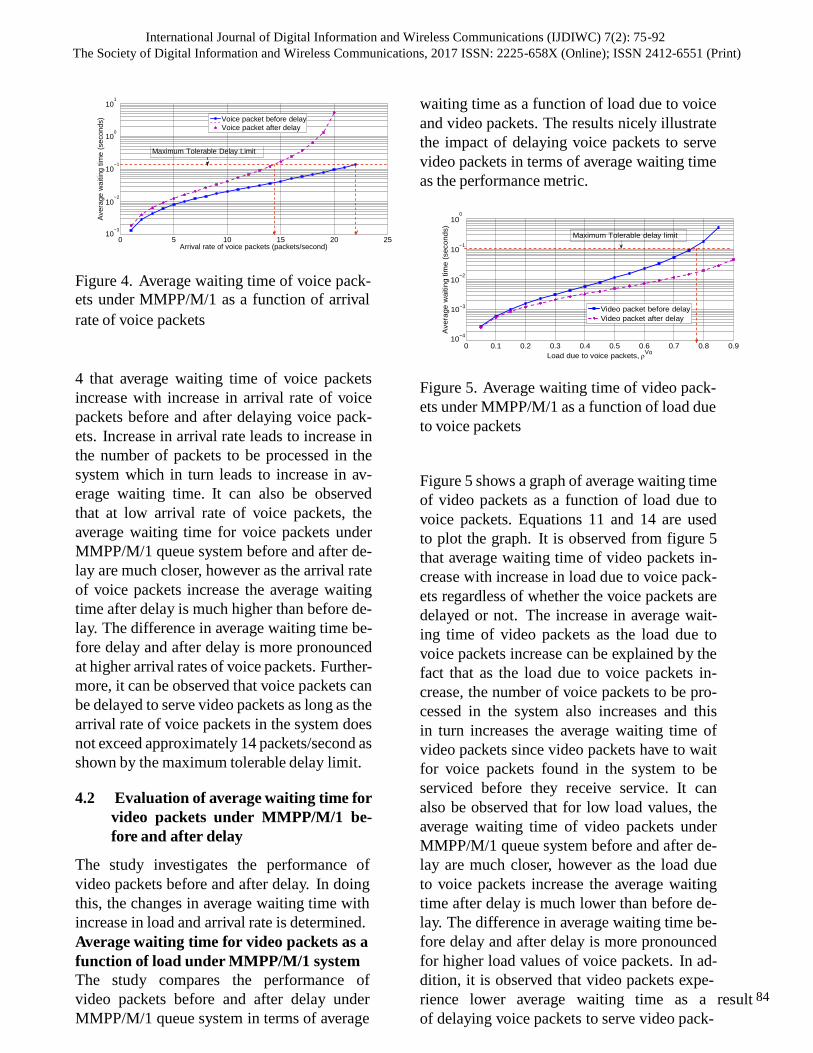
International Journal of Digital Information and Wireless Communications (IJDIWC) 7(2): 75-92
The Society of Digital Information and Wireless Communications, 2017 ISSN: 2225-658X (Online); ISSN 2412-6551 (Print)
Avera
ge w
aitin
g t
ime (
se
co
nds)
Avera
ge
waitin
g t
ime
(seco
nd
s)
10
10
−3
1
10
Voice packet before delay
Voice packet after delay 0
10
Maximum Tolerable Delay Limit
−1
10
waiting time as a function of load due to voice
and video packets. The results nicely illustrate
the impact of delaying voice packets to serve
video packets in terms of average waiting time
as the performance metric. −2
10
0
10
−3 10
0 5 10 15 20 25 Arrival rate of voice packets (packets/second) −1
Maximum Tolerable delay limit
Figure 4. Average waiting time of voice pack- −2
ets under MMPP/M/1 as a function of arrival 10
rate of voice packets
Video packet before delay
Video packet after delay
−4 10
4 that average waiting time of voice packets
increase with increase in arrival rate of voice
packets before and after delaying voice pack-
ets. Increase in arrival rate leads to increase in
the number of packets to be processed in the
system which in turn leads to increase in av-
erage waiting time. It can also be observed
that at low arrival rate of voice packets, the
average waiting time for voice packets under
MMPP/M/1 queue system before and after de-
lay are much closer, however as the arrival rate
of voice packets increase the average waiting
time after delay is much higher than before de-
lay. The difference in average waiting time be-
fore delay and after delay is more pronounced
at higher arrival rates of voice packets. Further-
more, it can be observed that voice packets can
be delayed to serve video packets as long as the
arrival rate of voice packets in the system does
not exceed approximately 14 packets/second as
shown by the maximum tolerable delay limit.
4.2 Evaluation of average waiting time for
video packets under MMPP/M/1 be-
fore and after delay
The study investigates the performance of
video packets before and after delay. In doing
this, the changes in average waiting time with
increase in load and arrival rate is determined.
Average waiting time for video packets as a
function of load under MMPP/M/1 system
The study compares the performance of
video packets before and after delay under
MMPP/M/1 queue system in terms of average
0 0.1 0.2 0.3 0.4 0.5 0.6 0.7 0.8 0.9
Load due to voice packets, ρVo
Figure 5. Average waiting time of video pack-
ets under MMPP/M/1 as a function of load due
to voice packets
Figure 5 shows a graph of average waiting time
of video packets as a function of load due to
voice packets. Equations 11 and 14 are used
to plot the graph. It is observed from figure 5
that average waiting time of video packets in-
crease with increase in load due to voice pack-
ets regardless of whether the voice packets are
delayed or not. The increase in average wait-
ing time of video packets as the load due to
voice packets increase can be explained by the
fact that as the load due to voice packets in-
crease, the number of voice packets to be pro-
cessed in the system also increases and this
in turn increases the average waiting time of
video packets since video packets have to wait
for voice packets found in the system to be
serviced before they receive service. It can
also be observed that for low load values, the
average waiting time of video packets under
MMPP/M/1 queue system before and after de-
lay are much closer, however as the load due
to voice packets increase the average waiting
time after delay is much lower than before de-
lay. The difference in average waiting time be-
fore delay and after delay is more pronounced
for higher load values of voice packets. In ad-
dition, it is observed that video packets expe-
rience lower average waiting time as a result 84
of delaying voice packets to serve video pack-
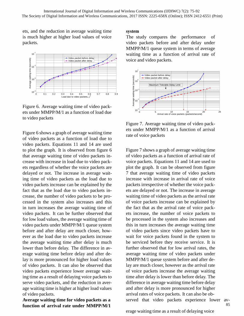
International Journal of Digital Information and Wireless Communications (IJDIWC) 7(2): 75-92
The Society of Digital Information and Wireless Communications, 2017 ISSN: 2225-658X (Online); ISSN 2412-6551 (Print)
Avera
ge w
aitin
g t
ime (
se
co
nds)
Avera
ge w
aitin
g t
ime (
se
co
nds)
ets, and the reduction in average waiting time
is much higher at higher load values of voice
packets.
−1
10
Video packet before delay
Video packet after delay
system
The study compares the performance of
video packets before and after delay under
MMPP/M/1 queue system in terms of average
waiting time as a function of arrival rate of
voice and video packets.
−2
10
1
10
−3
10 0
10
Video packet before delay
Video packet after delay
Maximum Tolerable Delay Limit
−1
−4 10 10
0 0.1 0.2 0.3 0.4 0.5 0.6 0.7 0.8 0.9
Load due to video packets, ρV
Figure 6. Average waiting time of video pack-
ets under MMPP/M/1 as a function of load due
to video packets
−2
10
−3
10 0 5
Arrival rate
10
of voice
15 20 25
packets (packets/second)
Figure 6 shows a graph of average waiting time
of video packets as a function of load due to
video packets. Equations 11 and 14 are used
to plot the graph. It is observed from figure 6
that average waiting time of video packets in-
crease with increase in load due to video pack-
ets regardless of whether the voice packets are
delayed or not. The increase in average wait-
ing time of video packets as the load due to
video packets increase can be explained by the
fact that as the load due to video packets in-
crease, the number of video packets to be pro-
cessed in the system also increases and this
in turn increases the average waiting time of
video packets. It can be further observed that
for low load values, the average waiting time of
video packets under MMPP/M/1 queue system
before and after delay are much closer, how-
ever as the load due to video packets increase
the average waiting time after delay is much
lower than before delay. The difference in av-
erage waiting time before delay and after de-
lay is more pronounced for higher load values
of video packets. It can also be observed that
video packets experience lower average wait-
ing time as a result of delaying voice packets to
serve video packets, and the reduction in aver-
age waiting time is higher at higher load values
of video packets.
Average waiting time for video packets as a
function of arrival rate under MMPP/M/1
Figure 7. Average waiting time of video pack-
ets under MMPP/M/1 as a function of arrival
rate of voice packets
Figure 7 shows a graph of average waiting time
of video packets as a function of arrival rate of
voice packets. Equations 11 and 14 are used to
plot the graph. It can be observed from figure
7 that average waiting time of video packets
increase with increase in arrival rate of voice
packets irrespective of whether the voice pack-
ets are delayed or not. The increase in average
waiting time of video packets as the arrival rate
of voice packets increase can be explained by
the fact that as the arrival rate of voice pack-
ets increase, the number of voice packets to
be processed in the system also increases and
this in turn increases the average waiting time
of video packets since video packets have to
wait for voice packets found in the system to
be serviced before they receive service. It is
further observed that for low arrival rates, the
average waiting time of video packets under
MMPP/M/1 queue system before and after de-
lay are much closer, however as the arrival rate
of voice packets increase the average waiting
time after delay is lower than before delay. The
difference in average waiting time before delay
and after delay is more pronounced for higher
arrival rates of voice packets. It can also be ob-
served that video packets experience lower av-
85
erage waiting time as a result of delaying voice

International Journal of Digital Information and Wireless Communications (IJDIWC) 7(2): 75-92
The Society of Digital Information and Wireless Communications, 2017 ISSN: 2225-658X (Online); ISSN 2412-6551 (Print)
−4
Avera
ge w
aitin
g t
ime (
se
co
nds)
Avera
ge w
aitin
g t
ime (
se
co
nds)
packets to serve video packets, and the reduc-
tion in average waiting time is much higher at
higher arrival rates of voice packets. Further-
more, it can be observed that video packets can
be delayed to serve video packets as long as the
arrival rate of voice packets in the system does
not exceed approximately 14 packets/second.
1
10
Video packet before delay Video packet after delay
0
10
Maximum Tolerable Delay Limit
−1
10
−2
10
−3
10 0 5 10 15 20 25
Arrival rate of video packets (packets/second)
Figure 8. Average waiting time of video pack-
ets under MMPP/M/1 as a function of arrival
rate of video packets
Figure 8 shows a graph of average waiting time
of video packets as a function of arrival rate of
video packets. Equations 11 and 14 are used to
plot the graph. It can be observed from figure
8 that average waiting time of video packets
increase with increase in arrival rate of video
packets regardless of whether the voice pack-
not exceed approximately 21 packets/second.
4.3 Evaluation of average waiting time for
voice packets under MMPP/BP/1 be-
fore and after delay
In this study, the performance of voice pack-
ets before and after delay under MMPP/BP/1
queue system in terms of average waiting time
as a function of load and arrival rate are com-
pared. The results nicely illustrate the impact
of delaying voice packets to serve video pack-
ets in terms of average waiting time as the per-
formance metric.
4.4 Average waiting time for voice pack-
ets as a function of load under
MMPP/BP/1 system
The study compares the performance of
voice packets before and after delay under
MMPP/BP/1 queue system in terms of average
waiting time as a function of load due to voice
and video packets.
10
0
Maximum Tolerable Delay Limit
10
−1
10
−2
ets are delayed or not. The increase in aver-
age waiting time of video packets as the arrival
10
−3
Voice packet before delay
Voice packet after delay
rate of video packets increase can be explained
by the fact that as the arrival rate of video
packets increase, the number of video pack-
ets to be processed in the system also increases
which results into increase in the average wait-
ing time of video packets. It can also be ob-
served that for low arrival rates of video pack-
ets, the average waiting time of video packets
under MMPP/M/1 queue system before and af-
ter delay are closer, however as the arrival rate
of video packets increase the average waiting
time after delay is lower than before delay. The
difference in average waiting time before delay
and after delay is more pronounced for higher
arrival rates of video packets. In addition, it
can be observed that video packets can be de-
layed to serve video packets as long as the ar-
rival rate of video packets in the system does
10 0 0.1 0.2 0.3 0.4 0.5 0.6 0.7 0.8 0.9
Load due to voice packets, ρVo
Figure 9. Average waiting time of voice pack-
ets under MMPP/BP/1 as a function of load
due to voice packets
Figure 9 shows a graph of average waiting time
of voice packets as a function of load due to
voice packets under MMPP/BP/1 queue sys-
tem. Equations 17 and 23 are used to plot the
graph. It can be observed from figure 9 that
average waiting time of voice packets increase
with increase in load due to voice packets re-
gardless of whether the voice packets are de-
layed or not. The increase in average waiting
time of voice packets as the load due to voice
86
packets increase can be explained by the fact

International Journal of Digital Information and Wireless Communications (IJDIWC) 7(2): 75-92
The Society of Digital Information and Wireless Communications, 2017 ISSN: 2225-658X (Online); ISSN 2412-6551 (Print)
Avera
ge w
aitin
g t
ime (
se
co
nds)
that as the load due to voice packets increase,
the number of voice packets to be processed
in the system also increases and this in turn in-
creases the average waiting time of voice pack-
ets. Furthermore, it can be observed that for
low load values, the average waiting time of
voice packets under MMPP/BP/1 queue sys-
tem before and after delay are much closer,
however as the load due to voice packets in-
crease the average waiting time after delay is
much higher than before delay. The difference
in average waiting time before delay and af-
ter delay is more pronounced for higher load
values of voice packets. It can also be ob-
served that voice packets can be delayed to
serve video packets as long as the load due to
voice packets does not exceed 81% as shown
by the maximum tolerable delay limit.
Average waiting time for voice packets as a
function of arrival rate under MMPP/BP/1
system
Comparison of the performance of voice pack-
ets before and after delay under MMPP/BP/1
queue system in terms of average waiting time
as a function of arrival rate of voice and video
packets.
1
10
Voice packet before delay
Voice packet after delay 0
10
Maximum Tolerable Delay Limit
−1
10
−2
10
−3
10 0 5 10 15 20 25
Arrival rate of voice packets, (packets/second)
Figure 10. Average waiting time of voice pack-
ets under MMPP/BP/1 as a function of arrival
rate of voice packets
Figure 10 shows a graph of average waiting
time of voice packets as a function of arrival
rate of voice packets under MMPP/BP/1 queue
system. Equations 17 and 23 are used to plot
the graph. It can be observed from figure 10
that average waiting time of voice packets in-
crease with increase in arrival rate of voice
packets regardless of whether the voice pack-
ets are delayed or not. The increase in average
waiting time of voice packets as the arrival rate
of voice packets increase can be explained by
the fact that as the arrival rate of voice pack-
ets increase, the number of voice packets to be
processed in the system also increases and this
leads to increase in the average waiting time
of voice packets. It can further be observed
that for low arrival rate values of voice pack-
ets, the average waiting time of voice packets
under MMPP/BP/1 queue system before and
after delay are closer, however as the arrival
rate of voice packets increase the average wait-
ing time after delay is higher than before de-
lay. The difference in average waiting time
before delay and after delay is much higher
at higher arrival rate of voice packets. It can
also be observed that voice packets can be de-
layed to serve video packets as long as the ar-
rival rate of voice packets does not exceed 14
packets/second.
4.5 Evaluation of average waiting time for
video packets under MMPP/BP/1 be-
fore and after delaying voice packets
This study compares the performance of video
packets before and after delaying voice packets
under MMPP/BP/1 queue system in terms of
average waiting time.
Average waiting time for video packets as a
function of load under MMPP/BP/1 system
The study compares the performance of
video packets before and after delaying under
MMPP/BP/1 queue system in terms of average
waiting time as a function of load due to voice
and video packets.
Figure 11 shows a graph of average waiting
time of video packets as a function of load due
to voice packets under MMPP/BP/1 queue sys-
tem. Equations 20 and 26 are used to plot the
graph. It can be observed from figure 11 that
average waiting time of voice packets increase
with increase in load due to voice packets ir-
respective of whether the voice packets are de-
layed or not.
It can further be observed that for low load val-
ues of video packets, the average waiting time
87
of voice packets under MMPP/BP/1 queue sys-

International Journal of Digital Information and Wireless Communications (IJDIWC) 7(2): 75-92
The Society of Digital Information and Wireless Communications, 2017 ISSN: 2225-658X (Online); ISSN 2412-6551 (Print)
Avera
ge w
aitin
g t
ime (
se
co
nds)
Avera
ge w
aitin
g t
ime (
se
co
nds)
Avera
ge w
aitin
g t
ime (
se
co
nds)
10
1
10
0
10
Maximum Tolerable Delay Limit
−1
10
−2
10
−3 Video packet before delay
Video packet after delay
−4
10 0 0.1 0.2 0.3 0.4 0.5 0.6 0.7 0.8 0.9
Load due to voice packets, ρVo
Figure 11. Average waiting time of video pack-
ets under MMPP/BP/1 as a function of load
due to voice packets
tem before and after delay are closer, however
as the load due to voice packets increase the
average waiting time after delay is lower than
before delay. The difference in average waiting
time before delay and after delay is higher at
higher arrival rates of voice packets. It can also
be observed that voice packets can be delayed
to serve video packets even when the load due
to voice packets is approximately 90%.
−1
10
packets increase can be explained by the fact
that as the load due to video packets increase,
the number of video packets to be processed
in the system also increases and this in turn in-
creases the average waiting time of video pack-
ets. It can further be observed that for low
load values of video packets, the average wait-
ing time of video packets under MMPP/BP/1
queue system before and after delay are much
closer, however as the load due to video pack-
ets increase the average waiting time after de-
lay is lower than before delay. The difference
in average waiting time before delay and after
delay increases as the load due to video pack-
ets increase. It can also be observed that voice
packets can be delayed to serve video packets
without restrictions on the load due to video
packets.
Average waiting time for video packets as a
function of arrival rate under MMPP/BP/1
system
The study compares the performance of
video packets before and after delaying under
MMPP/BP/1 queue system in terms of aver-
age waiting time as a function of arrival rate of voice and video packets.
Video packet before delay
Video packet after delay
−2
10 10
0
10 −3
10
Video packet before delay
Video packet after delay
Maximum Tolerable Delay Limit
−1
10
−4 10
0 0.1 0.2 0.3 0.4 0.5 0.6 0.7 0.8 0.9
Load due to video packets, ρV −2
Figure 12. Average waiting time of video pack-
ets under MMPP/BP/1 as a function of load
due to video packets
Figure 12 shows a graph of average waiting
time of video packets as a function of load due
to video packets under MMPP/BP/1 queue sys-
tem. Equations 20 and 26 are used to plot the
graph. It can be observed from figure 12 that
average waiting time of video packets increase
with increase in load due to video packets re-
gardless of whether the voice packets are de-
layed or not. The increase in average waiting
time of video packets as the load due to video
−3
10 0 5 10 15 20 25
Arrival rate of voice packets (packets/second)
Figure 13. Average waiting time of video pack-
ets under MMPP/BP/1 as a function of arrival
rate of voice packets
Figure 13 shows a graph of average waiting
time of video packets as a function of arrival
rate of voice packets under MMPP/BP/1 queue
system. Equations 17 and 23 are used to plot
the graph. It can be observed from figure 13
that average waiting time of video packets in-
crease with increase in arrival rate of voice
88
packets regardless of whether the voice pack-

International Journal of Digital Information and Wireless Communications (IJDIWC) 7(2): 75-92
The Society of Digital Information and Wireless Communications, 2017 ISSN: 2225-658X (Online); ISSN 2412-6551 (Print)
Avera
ge w
aitin
g t
ime (
se
co
nds)
Avera
ge w
aitin
g t
ime (
se
co
nds)
Avera
ge w
aitin
g t
ime (
se
co
nds)
ets are delayed or not. The increase in average
waiting time of video packets as the arrival rate
of voice packets increase can be explained by
the fact that as the arrival rate of voice pack-
ets increase, the number of voice packets to be
processed in the system also increases and this
leads to increase in the average waiting time
of video packets since video packets have to
wait for voice packets found in the system to be
serviced before video packets can get serviced.
It can further be observed that for low arrival
rate values of voice packets, the average wait-
ing time of video packets under MMPP/BP/1
queue system before and after delay are closer,
however as the arrival rate of voice packets in-
crease the average waiting time after delay is
lower than before delay. The difference in av-
erage waiting time before delay and after delay
is much higher at higher arrival rate of voice
packets. It can also be observed that voice
packets can be delayed to serve video packets
for arrival rates of voice packets of upto ap-
proximately 22 packets/second.
1
10
Video packet before delay
Video packet after delay 0
10
Maximum Tolerable Delay Limit
−1
10
−2
10
−3
10 0 5 10 15 20 25
Arrival rate of video packets (packets/second)
Figure 14. Average waiting time of video pack-
the fact that as the arrival rate of video pack-
ets increase, the number of video packets to be
processed in the system also increases and this
leads to increase in the average waiting time
of video packets. It can further be observed
that for low arrival rate values of video pack-
ets, the average waiting time of video packets
under MMPP/BP/1 queue system before and
after delay are closer, however as the arrival
rate of video packets increase the average wait-
ing time after delay is lower than before de-
lay. The difference in average waiting time
before delay and after delay is much higher
at higher arrival rate of video packets. It can
also be observed that voice packets can be de-
layed to serve video packets for arrival rates of
video packets of upto approximately 22 pack-
ets/second.
Next, the tradeoff in improvement in perfor-
mance of video packets against degradation in
service of voice packets under MMPP/M/1 is
evaluated.
4.6 Tradeoff in improvement in perfor-
mance of video packets and degrada-
tion in service of voice packets under
MMPP/M/1
The study investigates the tradeoff in improve-
ment in performance of video packets against
the degradation in performance of voice pack-
ets in terms of average waiting time as a func-
tion of load and arrival rate under MMPP/M/1
queue system.
ets under MMPP/BP/1 as a function of arrival
rate of video packets
0
10 Voice packet before delay
Voice packet after delay
0
10 Video packet before delay
Video packet after delay
−1 −1
10 10
Figure 14 shows a graph of average waiting
time of video packets as a function of arrival
rate of video packets under MMPP/BP/1 queue
system. Equations 17 and 23 are used to plot
the graph. We observe from figure 14 that av-
−2
10
−3
10
−4
10 0 0.2 0.4 0.6 0.8
Load due to voice packets, ρVo
−2
10
−3
10
−4
10 0 0.2 0.4 0.6 0.8
Load due to voice packets, ρVo
erage waiting time of video packets increase
with increase in arrival rate of video packets
irrespective of whether the voice packets are
delayed or not. The increase in average wait-
ing time of video packets as the arrival rate
of video packets increase can be explained by
Figure 15. Average waiting time of voice and
video packets under MMPP/M/1 as a function
of load due to voice packets
89
Figure 15 shows a graph of average waiting

International Journal of Digital Information and Wireless Communications (IJDIWC) 7(2): 75-92
The Society of Digital Information and Wireless Communications, 2017 ISSN: 2225-658X (Online); ISSN 2412-6551 (Print)
(packets/second)
Avera
ge
waitin
g t
ime
(seco
nd
s)
Avera
ge
waitin
g t
ime
(seco
nd
s)
Avera
ge w
aitin
g t
ime (
se
co
nds)
Avera
ge w
aitin
g t
ime (
se
co
nds)
time of voice and video packets as a function
of load due to voice packets under MMPP/M/1
queue system. Equations 9 and 12, 11 and
14 are used to plot the graph. It can be ob-
served from figure 15 that average waiting time
of both voice and video packets increase with
increase in load due to voice packets irrespec-
tive of whether the voice packets are delayed or
not. It can further be observed that video pack-
ets experience a higher improvement in perfor-
mance as a result of reduced average waiting
time, for example, at the load of 0.4 the aver-
age waiting time is reduced by 0.0028 seconds
while the increase in average waiting time of
voice packets at the same load is increased by
0.001 seconds. A similar trend is observed at
a load of o.6 where the reduction in average
waiting time of video packets is 0.014 while
the increase in average waiting time of voice
packets is 0.005 seconds. It can also be ob-
served that voice packets can be delayed to
serve video packets as long as the load due to
voice packets does not exceed 81%.
ets experience a higher improvement in perfor-
mance as a result of reduced average waiting
time, for example, at the arrival rate of 5 pack-
ets/second the average waiting time is reduced
by 0.005 seconds while the increase in aver-
age waiting time of voice packets at the same
arrival rate is increased by 0.004 seconds. A
similar trend is observed at a arrival rate of 10
packets/second where the reduction in average
waiting time of video packets is 0.03 while the
increase in average waiting time of voice pack-
ets is 0.02 seconds. It can also be observed that
voice packets can be delayed to serve video
packets as long as the arrival rate of voice pack-
ets does not exceed 14 packets/second.
4.7 Tradeoff in improvement in perfor-
mance of video packets and degrada-
tion in service of voice packets under
MMPP/BP/1
The study investigates the tradeoff in improve-
ment in performance of video packets against
the degradation in performance of voice pack-
ets in terms of average waiting time as a 1
10
Voice packet before delay
Voice packet after delay
0
10
1 10
Video packet before delay
Video packet after delay
0
10
function of load and arrival rate under the
MMPP/BP/1 queue system.
−1 −1
10 10
−2 −2
10 10
0
10
Voice packet before delay
Voice packet after delay −1
10
0
10
Video packet before delay
Video packet after delay −1
10
−3
10 0 5 10 15 20 25
−2 −2
−3 10 10
10 0 5 10 15 20 25
Arrival rate of voice packets (packets/second) Arrival rate of voice packets
Figure 16. Average waiting time of voice and
video packets under MMPP/M/1 as a function
of arrival rate of voice packets
−3
10
−4
10 0 0.2 0.4 0.6 0.8
Load due to voice packets, ρVo
−3
10
−4
10 0 0.2 0.4 0.6 0.8
Load due to voice packets, ρVo
Figure 16 shows a graph of average waiting
time of voice and video packets as a function of
arrival rate of voice packets under MMPP/M/1
queue system. Equations 9 and 12, 11 and
14 are used to plot the graph. It can be ob-
served from figure 16 that average waiting time
of both voice and video packets increase with
increase in arrival rate of voice packets regard-
less of whether the voice packets are delayed or
not. It can further be observed that video pack-
Figure 17. Average waiting time of voice and
video packets under MMPP/BP/1 as a function
of load due to voice packets
Figure 17 shows a graph of average waiting
time of voice and video packets as a function of
load due to voice packets under MMPP/BP/1
queue system. Equations 17 and 17, 20 and
20 are used to plot the graph. It can be ob-
served from figure 17 that average waiting time
90
of both voice and video packets increase with

International Journal of Digital Information and Wireless Communications (IJDIWC) 7(2): 75-92
The Society of Digital Information and Wireless Communications, 2017 ISSN: 2225-658X (Online); ISSN 2412-6551 (Print)
Avera
ge w
aitin
g t
ime (
se
co
nds)
Avera
ge w
aitin
g t
ime (
se
co
nds)
increase in load due to voice packets regard-
less of whether the voice packets are delayed or
not. It can further be observed that video pack-
ets experience a higher improvement in per-
formance as a result of reduced average wait-
ing time, for example, at the load 0.4 the av-
erage waiting time is reduced by 0.0025 sec-
onds while the increase in average waiting time
of voice packets at the same arrival rate is in-
creased by 0.0008 seconds. A similar trend is
observed at a load of 0.6 where the reduction in
average waiting time of video packets is 0.014
while the increase in average waiting time of
voice packets is 0.004 seconds. It can also be
observed that voice packets can be delayed to
serve video packets as long as the load does not
exceed 81%.
is observed at arrival rate of 10 packets/second
where the reduction in average waiting time of
video packets is 0.02 while the increase in av-
erage waiting time of voice packets is 0.017
seconds. Note also that voice packets can be
delayed to serve video packets as long as the
arrival rate does not exceed 15 packets/second.
5 CONCLUSION
This study proposes an improved LLQ algo-
rithm which delays voice packets that arrive
while the video packets are already in the
queue and services video packets as long as
the voice packets are not delayed beyond the
maximum tolerable delay limits. The algo-
rithm is modeled using the MMPP/G/1 queue
system. Two special cases of MMPP/G/1 are 1
10
Voice packet before delay
1
10
Video packet before delay used, that is, MMPP/M/1 and MMPP/BP/1
Voice packet after delay Video packet after delay which exhibit correlated arrivals and exponen- 0
10
−1
10
−2
10
−3
10 0 5 10 15 20 25
0
10
−1
10
−2
10
−3
10 0 5 10 15 20 25
tial and Bounded Pareto service times respec-
tively. We developed analytical models which
enables us to investigate the trade-offs existing
between the increase in delay experienced by
voice packets as a result of delay and the de- lay reduction experienced by video packets as
Arrival rate of voice packets, (packets/second) Arrival rate of voice packets (packets/second)
Figure 18. Average waiting time of voice and
video packets under MMPP/BP/1 as a function
of arrival rate of voice packets
Figure 18 shows a graph of average waiting
time of voice and video packets as a function of
arrival rate of voice packets under MMPP/BP/1
queue system. Equations 17 and 17, 20 and
20 are used to plot the graph. It can be ob-
served from figure 18 that average waiting time
of both voice and video packets increase with
increase in arrival rate of voice packets regard-
less of whether the voice packets are delayed or
not. It can further be observed that video pack-
ets experience a higher improvement in per-
formance as a result of reduced average wait-
ing time, for example, at arrival rate of 5pack-
ets/second the average waiting time is reduced
by 0.003 seconds while the increase in aver-
age waiting time of voice packets at the same
arrival rate is 0.004 seconds. A similar trend
a result of delaying voice packets. The numer-
ical results obtained from the derived models
show that delaying voice packets leads to re-
duction in the average waiting time of video
packets and an increase in the average waiting
time of voice packets, however the reduction in
average waiting time of video packets is higher
than the increase in the average waiting time
of voice packets. Furthermore, the voice pack-
ets can be delayed to serve video packets as
long as the load and arrival rates of voice pack-
ets does not exceed 81% and 14 packets/second
respectively.
REFERENCES
[1] P. Jumnani, M. Zaveri, ”A Novel Cross-Layer Ar-
chitecture for Video Streaming Over MANET,” in
Proc. Ninth International Conference on Wireless
Communication and Sensor Networks, 2014.
[2] M. Veeralakshmi, R. Pugazendi, ”Depiction of
Routing Protocols in Mobile Adhoc Networks: Be- 91
haviour Analysis,” in International Journal of Com-

International Journal of Digital Information and Wireless Communications (IJDIWC) 7(2): 75-92
The Society of Digital Information and Wireless Communications, 2017 ISSN: 2225-658X (Online); ISSN 2412-6551 (Print)
puter Science and Mobile Computing. Volume 2(8),
August 2013, pp.96-101.
[3] K. Bora, ”Efficient Use of Resources in Mobile Ad
Hoc Networks”, ( Ph.D. dissertation, University of
Rochester, New York), 2013.
[4] K. Wallance, ”Authorized Self-Study Guide-Cisco
Voice over IP (CVOICE)”, Cisco Press, 2010.
[5] K. Semeria, ”Supporting Differentiated Service
Classes: Queue Scheduling Disciplines”, Juniper
Networks, Inc, 2001.
[6] H. Tetsuji, ”Analysis of Multiclass Feedback
Queues and its Application to a Packet Scheduling
Problem,” Journal of Industrial and Management
Optimization, Volume 6(3), 2010, pp.541-568.
[7] B. Dekeris, T. Adomkus, and A. Budnikas, ”Analy-
sis of QoS Assurance Using Weighted Fair Queue-
ing (WFQ) Scheduling Discipline with Low La-
tency Queue (LLQ), in Proc. International Confer-
ence on Information Technology, Jun. 2006.
[8] P. Rukmani, R. Ganesen, ”Enhanced Low Latency
Queueing Algorithm for real Time Applications in
Wireless Networks,” International Journal of Tech-
nology, Volume 7(4), 2016. pp. 663-672.
[9] L. Kleinrock .Queueing Systems, Volume I & II.
Computer Applications. John Wiley & Sons, 1976..
[10] E. Glenbe, G. Pujolle, J.C. Nelson, ”Introduction
to Queuing Networks,” John Wiley and Sons, 1987.
[11] B. K. Asingwire, M. Okopa, T. Bulega, ”Model-
ing Performance of VoIP Traffic over 802.11 Wire-
less Mesh Network Under Correlated Inter-arrival
Times,” In the International Journal of Digital Infor-
mation and Wireless Communications (IJDIWC),
Volume 6(2)May 2016. pp. 122-138.
[12] W. Fischer, K. Meier-Hellstern, ”The Markov-
modulated Poisson process (MMPP) cookbook”.
Proceedings of the Performance Evaluation, volume
18(2), Sep. 1993, pp. 149-171.
[13] B. Ciciani, A. Santoro, P. Romano, ”Approximate
Analytical Models for Networked Servers Subject
to MMPP Arrival Processes,” Proceedings of The
6th IEEE International Symposium on Network
Computing and Applications, 2007.
[14] N. Gans, G. Koole, A. Mandelbaum, ”Tele-
phone Call Centers: Tutorial, Review, and Re-
search Prospects,” Proceedings of the Manufactur-
ing & Service Operations Management, volume
2(5), 2003.
[15] A. O. Allen, ”Probability, Statistics and Queuing
Theory, with computer Science Applications,” Aca-
demic Press, Boston., 2nd edition, 1990.
[16] H. Li, M. Muskulus, L. Wolters, ”Modeling Job
Arrivals in adata-intensive Grid,” Proceeding of the
12th Workshop on Job Scheduling Strategies for
Parallel Processing, 2006.
[17] ITU-T Recommendation G.114, ”International
telephone connections and circuits-General Recom-
mendations on the transmission quality for an en-
tire international telephone connection,” ITU-T G-
SERIES RECOMMENDATIONS, 2003.
[18] P. Rohal1, R. Dahiya, P. Dahiya, ”Study and Anal-
ysis of Throughput, Delay and Packet Delivery Ra-
tio in MANET for Topology Based Routing Proto-
cols (AODV, DSR and DSDV. In the International
Journal for Advance Research in Engineering and
Technology. Volume 1(II). 2013, pp. 54-58.
[19] R. Kumar, M. Misra, A. K. Sarje, ”A Simplified
Analytical Model for End-To-End Delay Analysis
in MANET,” In nternational Journal of Computer
Applications-IJCA, 2010, pp. 195-199.
[20] P. I. Basarkod, S. S. Manvi, ”On-demand QoS
and Stability Based Multicast Routing in Mobile Ad
Hoc Networks,” In International Journal of Elec-
tronics and Telecommunications, Volume 60(1).
2014, PP. 27-39.
92

International Journal of Digital Information and Wireless Communications (IJDIWC) 7(2): 93-105
The Society of Digital Information and Wireless Communications, 2017 ISSN: 2225-658X (Online); ISSN 2412-6551 (Print)
93
Mining Top-T Web Traversal Subsequences Santosh Kumar* and Neha Tyagi
Department of Computer Science and Engineering
Krishna Institute of Engineering and Technology, Ghaziabad, India
ABSTRACT
There is rapid growth in the information over the
internet from extensive range of sources thereby
leading to information overload problem. Web
mining is being used as solution to this problem. As
website contains a large number of pages related to
the same information. User has to traverse a sequence
of web pages in search of relevant and required
information. The traversal sequences of user show
the user interest and habit. These traversal sequences
could be used to reorganization website structure,
thereby presenting the needed and important
information to the user in a few clicks. In this paper,
genetic algorithm is applied to find the Top-T
traversal subsequences useful for reorganizing the
website structure. It has been experimentally shown
as the proposed algorithm is able to select better Top-
T traversal subsequences than the existing
Incremental Pattern Mining Algorithm.
KEYWORDS
Web Mining, Web Data, Web Content, Web Usage,
Web Structure, Information Extraction, User
Traversal Sequence.
1. INTRODUCTION
World Wide Web (WWW) is a huge source of
information that is being uploaded/updated
dynamically from various sources over the
internet. Web mining techniques have been
proven to be efficient for information extraction.
The data mining techniques are applied on web
data, is known as Web Mining [1]. Web mining
broadly classified into three: Web Content
Mining, Web structure Mining, and Web Usage
Mining [2], [3]. Web Content Mining used web
data such as text, multimedia etc. to extract
information that is useful to the user [4]. Web
Structure mining focused to the structure of the
web page or website and used this information
about the structure of the web to extract useful
information [5]. Web Usage Mining used log
data that contain the information about the user
and its access behavior, which helps to extract
useful information based on user query [6].
Understanding of user access pattern helps the
business manager to reorganize the website
structure, thereby improving their business. A
website with „n‟ web pages can be described by
a graph „G‟ called as web graph, where nodes
represent the web pages and edges represent the
hyperlinks or links between the web pages. A
traversal sequence „S‟ (or user navigational
pattern or web navigational pattern) is a set of
web pages visited by the user in a single visit (or
session), <s1,s2,s3……> where s1, s2, s3,….. are
the web pages. Mining the traversal pattern of
user‟s navigational behavior is called as traversal
pattern mining. Web logs contain all the
essential information about user and this
information is used to discover user‟s access
patterns for web traversal pattern mining [7], [8],
[9]. It helps web site designer to improve the
design and performance of the web site leading
to better decision making [10]. As many
websites have hundreds of web pages and it
cannot be possible to traverse all the web pages
in searching of required information. Website
reorganization is a better solution to this problem
as it improves web navigation efficiency. The
information in the website is presented in the
form needed by the user. Although a designers
develop website for a particular goal but it is
used for the different purposes by different users,
and to make this use efficient the website should
serve the user as per their requirements. The
ultimate goal of website reorganization is to help
the user so that in fewer clicks they can access
desired information. To do so there is the
necessity to place highly accessed web pages
closer to the home page as well as less accessed
web pages a little far away from the home page
in website structure. While searching for desired
information, sometimes user has to traverse a
long path which is time consuming traversal.
The traversal time could be minimized if website
is well organized. In well organized websites the
highly accessed web pages remain on top in the
hierarchical structure of website structure. Home
page is the top of hierarchy. An enormous

International Journal of Digital Information and Wireless Communications (IJDIWC) 7(2): 93-105
The Society of Digital Information and Wireless Communications, 2017 ISSN: 2225-658X (Online); ISSN 2412-6551 (Print)
94
amount of web users, browse website to find
required information and the navigation should
be easy so that the user can find the information
quickly [11]. The significant information about
the user‟s interest, habits, hobbies etc., can be
obtained by analyzing the access pattern of the
user, and this information is very useful for the
up-gradation of the website. The performance of
any website depends on the up-gradation of
website. Mining results could be use to improve
the structure of the website and also its access
efficiency. Traversal pattern mining is the
process of mining user navigational patterns to
help the user so that user can easily access the
desired information. In traversal pattern mining,
user traversal patterns are the input for finding
frequently traversed web pages. Traversal
pattern mining is categorized into Path Traversal
Pattern Mining and Web Traversal Pattern
Mining on the basis of simple and non-simple
traversal patterns respectively [10]. Simple
traversal patterns are restricted with the
appearance of pages that only once, a page can
appear in the traversal pattern, and consider the
forward references only. On the other hand, non-
simple traversal patterns do not bother the
number of appearance of any page in the
traversal pattern so that a page may appears
more than once, backward references are also
consider along with forward references that
make non-simple traversal patterns sufficient for
web environment unlike simple traversal
patterns. Sequential pattern mining is quiet
similar to web traversal pattern mining,
introduced in [12], and it is very important for
determining the time related behavior and also to
obtain the information which is used in
prediction of user access patterns, marketing, e-
commerce etc. Sequence pattern mining could
find hidden information and also helps in
decision making [10]. Web traversal pattern
mining problem is all about to find the maximal
sequences that maintain the minimum support
count, from the given dataset. The input for web
traversal pattern mining is user traversal
sequences and minimum support count that
specified by user in terms of percentage for e.g.
50%, 60%, 80% etc. On the basis of these
traversal sequences the website can be
reorganized as highly visited web pages placed
near to the home page and less visited web pages
placed a little far away from the home page
thereby improving the performance and
efficiency of the website.
2. RELATED WORK
Website designer use Path Traversal Pattern
Mining Techniques [13], [14], [15], [16] to
discover user‟s navigational behavior. These
extracted navigational patterns are used to
improve the design and performance of websites.
Existing algorithms are classified into: Simple
path traversal pattern mining algorithms and
Non- simple path traversal pattern mining
algorithms. Simple path traversal pattern mining
algorithms (Full Scan, FS [14], Selective Scan,
SS [14], Maintenance of Frequent Traversal
Patterns, MAFTP [16] and so on) are limited to
discover simple path traversal patterns where in
the traversal pattern a page can appear only once
with the consideration of forward references
only. On the other hand non-simple path
traversal pattern mining algorithms (Mining
Frequent Traversal Patterns, MFTP algorithm
[7], and Integrating Path traversal patterns and
Association rules, IPA algorithm [8], [9])
consider both forward and backward references
with the traversal pattern where a page can
appear more than once. When the database is
updated mining frequent sequence patterns are to
be calculated again. FS-Miner efficiently finds
the access sequence and constructs a FS-Tree for
sequence patterns. As FS-Miner has the
capability of accommodate to the modification
of user behavior it avoids the unnecessary re-
computation for new input sequences [17].
Incremental Sequence Lattice algorithm (ISL),
proposed in [18], is based on Sequential Pattern
Discovery using Equivalence classes that could
modify the grid structure of incremental
sequence lattice with the modification of
database. All the sequence patterns are stored in
the lattice and only the count of new generated
sequence patterns are to be calculated. IncWTP
(Incremental Web Traversal Pattern [10]) and
IntWTP (Interactive Web Traversal Pattern [10])
algorithms are used to maintain the web traversal
patterns when the database is updated and to find
the web traversal patterns when minimum
support is adjusted. Frequent traversal pattern
mining is very important as it helps to find out
the relationship among the different users access
behavior. Maximal Frequent Traversal Pattern
Mining (MFTPM) algorithm proposed in [19] is

International Journal of Digital Information and Wireless Communications (IJDIWC) 7(2): 93-105
The Society of Digital Information and Wireless Communications, 2017 ISSN: 2225-658X (Online); ISSN 2412-6551 (Print)
95
,
used to mine the set of maximal frequent
traversal pattern and also a tree structure to store
the frequent traversal patterns. MFTPM
algorithm restrain every page in the traversal
pattern by using the dwell time technique where
dwell time of any web page is the actual time
spend by the user on the content page, and
reduce the execution time and I/O cost.
3. WEB GRAPH AND WEB TRAVERSAL
PATTERNS
A web graph contains a large number of nodes
with few increments in web pages in future. A
survey stated that an average node has approx
seven hyperlinks to different web pages thus a
web graph contains several billion hyperlinks in
it [20]. As web graph is exponentially increases
thus it is very difficult to get the whole graph or
if it is possible then its storage and rapidly
changing behavior led to the challenges. Thus a
part of web graph is used for the study. Here in
this paper a sample web graph of website is used
and is shown in Figure 1. A website can be
easily shown in a graphical manner, where the
graph „G‟ is known as web graph in which the
nodes are the web pages and edges are the links
or hyperlinks within the web page or between the web pages.
subsequence of sequence S if it is a subset of S.
Let P and Q are two traversal sequences <0->3-
>2->4->1> and <3->2->4> respectively, here Q
is the subset of sequence P thus Q is a
subsequence. The Support Count of a
subsequence is defined as the occurrences of that
particular subsequence in the web traversal
sequence database. For example, let the
traversal sequences database is shown in Figure
2., and a subsequence (3->2->4) for which the
support count has to calculate.
S.No. Traversal Sequence (Database)
1 0-> 3->2->4 2 0-> 3->2->4 ->1 3 4->1->2 4 3->2->4 ->1->0 5 2->3->4->1->0 6 1->2->3->4
Figure 2. Web Traversal Sequences
In Figure 2, it is shown that the support count of
subsequence (3->2->4) is 3 as its occurrence is
found 3 times in the web traversal sequence
database. Mathematically, the support count can
be defined as Equation 1.
p
SupportCount = ∑Substring(SS,TSi )
i=1
0
(1)
where Substring(x,y) = 1 2
1 if y contains x
0 otherwise
and p is the no. of traversal sequences in the database.
3 4 The subsequence is said to be qualified
Figure 1. Web Graph of a Website
In Figure 1, a web graph „G‟ having nodes (0,
1,…., 4 ) and edges between them is shown. The
web traversal pattern or user traversal sequence
is the sequence of web pages traversed or visited
by the user in a particular session, stored in the
web logs and analyzes to understand the user‟s
interest and habit etc. Let S=<p1,p2,p3,….> a
web traversal pattern where p1, p2, p3,…. are
the web pages and the number of web pages in
the traversal pattern is called as the length of that
traversal sequence and the traversal sequence is
called as l-traversal sequence [15] where l is
length of traversal sequence. For e.g. , let a
traversal sequence <4->1->2> is a 3-traversal
sequence. A traversal sequence S′ is said to be a
subsequence if its support count is greater than
or equal to the minimum support count. A
qualified subsequence is the candidate
subsequence for the next level. Two candidate
subsequences „A‟ and „B‟ can be merged to
make new subsequence after satisfying the
condition of merging, e.g. let A=<a1,a2,….,an>
and B=<b1,b2,….,bm> be the two subsequences.
These two subsequences can be merged if
<a2,a3,….,an> is equal to <b1,b2,.…,bm-1> or
vice versa. Assuming two 2-sequence candidate
subsequences P and Q as <p1->p2> i.e. <3-
>2>and <q1->q2> i.e. <2->4> respectively, here
p2 is equal to q1 so the subsequences P and Q
can be merge together to form a new 3-sequence
subsequence <3->2->4>. In Figure 3, a lattice
structure is used to show the relationship

International Journal of Digital Information and Wireless Communications (IJDIWC) 7(2): 93-105
The Society of Digital Information and Wireless Communications, 2017 ISSN: 2225-658X (Online); ISSN 2412-6551 (Print)
96
between the traversal patterns and the structure
helps to find the relationship between two
patterns very quickly. If a user wants to explore
the traversal patterns containing web page „0‟,
then simply follow the structure from node „0‟.
from <0,1:12> here 0,1 is the subsequence and
12 is support count of it.
Website reorganization is a very important and
complex task, as it directly affects to the
importance of any website. The importance of
Figure 3. Simple Lattice Structure
A subsequence is said to be maximal if it is not
contained further by any other sequence. For e.g.
in Figure 3 there are several maximal
subsequences as <0,2>,<2,0>,<3,0>,….,<0,1,0>,
<0,1,2>,……<4,1,0,3> etc. Furthermore, a
lattice structure with support count of each
sequence is shown in Figure 4.
In Figure 4, each subsequence has its support
count associated with it, for e.g. let‟s take a node
well organized and up to date website is more
than the outdated website. The importance of
any website is depends on the content of the
website and the services provided by the website
to the user. Several parameters affect the
importance of website like number of visitors,
time spend by the user, query keyword
frequency etc. Higher the number of visitors
means there is likelihood of page containing the
Figure 4. Lattice Structure with Support Count

International Journal of Digital Information and Wireless Communications (IJDIWC) 7(2): 93-105
The Society of Digital Information and Wireless Communications, 2017 ISSN: 2225-658X (Online); ISSN 2412-6551 (Print)
97
relevant information to the users. If user stays for
a long time on particular page then there is
likelihood of page containing the important
information. A website should also adapt the
user searching behavior and changes itself
accordingly otherwise the importance of that
website will suffer and decrease. A website
contains large number of web pages and it is not
practically possible to put all the information on
a single web page. The different users have
different perception and requirement search of a
query, and it cannot feasible to serve billions of
queries by a single web page. So website has a
home page and a number of hyperlinks to other
web pages of the website. These hyperlinks
divert the user toward the different web pages of
that website. The frequent subsequences of any
website are those, which are traversed by the
user very frequently and indicate the traversal
behavior of the user. These frequent
subsequences also deduce that the web pages
included in the subsequences have the important
information. So there is need to find these
maximal frequent subsequences (Top-T
subsequences). The maximal common
subsequence is a problem of finding the longest
common subsequence in all the sequences of the
sequence database. Finding the longest common
subsequence is not similar to finding the
common substrings. Subsequences are not
necessarily to occupy the consecutive positions
within the sequences in the database. For
arbitrary number of input sequences this problem
is np-hard [21]. GA is capable to find solution to
np-hard problems. This paper addresses to find
Top-t traversal subsequences based on frequent
subsequences using GA. These Top-t traversal
subsequence can be used to reorganize the
website structure. The GA is briefly discussed
the next.
crossover, and mutation like basic genetic
operators reproduction, natural selection, and
variance of species. Algorithm starts with the
search of random set of solutions by applying
natural genetic operators in each generation. A
fitness value is assigned to each solution which
is further used to find the optimal solution of the
particular problem. GA is the mostly used
optimization method due to its global
perspective, simplicity, and parallel computing
etc. In GA a population of random solutions
called chromosomes is used on which three
natural genetic operators are applied until it
doesn‟t meet the termination condition. All these
three operators are discussed later in brief. A
simple genetic algorithm is shown in Figure 5,
described in [22].
Generate a population of random solutions
Population evaluated according to fitness function
Repeat until (termination condition)
Begin
Selection of parents to reproduce new offsprings
Perform crossover and mutation operators
Population evaluated according to fitness function
end
Figure 5. Simple Genetic Algorithm
4.1 Representation of Chromosome
Representation of chromosome is shown in
Figure 6. Here, each gene (like 2->4->0)
represents a 3-length subsequence of web
traversal pattern, and the numerical values
represent the node or web page and “→”
represents the linkage between two web pages. A
subsequence (2->4->0) shows the traversal of
user in which user firstly visit web page that is
uniquely identified by „2‟ then to „4‟ after that to
„0‟.
2->4->0 3->4->3 3->1->2 3->0->2 2->3->4 4->1->0 1->4->0 1->0->3 3->0->3 3->0->4
Figure 6. Representation of Chromosome
4. Genetic Algorithm
Genetic algorithm (GA) is a process that
employs evolutionary principles in living beings,
is a part of evolutionary algorithms (EA) class.
GA uses three principles of evolution: selection,
4.2 Fitness Function
In GA, fitness function is used to measure the
goodness of each solution represented by
chromosome. Using this fitness function a fitness
value is calculated for each candidate solution.
In proposed algorithm fitness value is calculated
using support count of each chromosome.

International Journal of Digital Information and Wireless Communications (IJDIWC) 7(2): 93-105
The Society of Digital Information and Wireless Communications, 2017 ISSN: 2225-658X (Online); ISSN 2412-6551 (Print)
98
2->4->0 3->4->3 4->0->1 0->2->0 1->0->1
2->3->2 4->2->1 3->1->2 3->0->2 2->3->4
Top-10 traversal subsequence Fitness
Value Subsequence 2->4->0 3->4->3 3->1->2 3->0->2 2->3->4 4->1->0 1->4->0 1->0->3 3->0->3 3->0->4 (6+3+
13+15) =37
Support Count 0 0 6 0 3 13 0 15 0 0
Figure 7. Fitness Value of Subsequence
Support count depends to the occurrence of
subsequence in the user traversal sequences
database. To calculate the support count of any
subsequence, the sequence database of web
traversal sequences is traversed for finding the
number of occurrences of that subsequence in
search of that particular subsequence so that the
occurrence of that subsequence can be counted.
Equation (1) is used to calculate the support
count of subsequence. The support count of
chromosome is a sum of support count of all the
genes of the chromosome. The fitness value of a
particular subsequence is shown in Figure 7.
4.3 Selection
It is a process of selecting individuals from the
population of randomly generated solutions to
perform crossover. Binary tournament selection
method [23] is used in the proposed algorithm.
Figure 8, shows binary tournament selection.
Take parameter k (let k=0.75)
Two individuals chosen randomly from the population
Choose a random number α between 0 and 1
If α<k Fitter individual is selected among them
Else
Less fitter individual is selected among them
Figure 8. Binary Tournament Selection Method [23]
In this two individuals are randomly chosen from
the population. A random value (say α) between
0 and 1, if the value of α is less than the value of
pre-defined value k (say k=0.75) then the
individual with higher fitness is selected
otherwise the individual with less fitness is
selected for crossover.
4.4 Crossover
Crossover is used for the reproduction of new off-
springs from the selected individuals for the
crossover. Crossover exchanges the genetic
substance of the parents. In literature, there exist
several crossover operators, of which single
point crossover operator is used here, in which a
randomly selected point is consider as crossover
point to perform crossover. The crossover
operation is shown in Figure 9 starts with the
calculation of crossover point CP as
CP=floor(T/2), where T is the number of genes
in a chromosome. After calculating the value of
CP new offsprings will generate in result of the
combination of two individuals in such a way
that the genes contained by offsprings will be
from one individual before CP and after CP from
the second individual.
4.5 Mutation
Mutation is used to modify one or more gene in
a chromosome. Mutation adds more genetic
diversity and also hinders the process of search
from slumping at any local optima. Figure 10,
shows random mutation. With the modification
of gene in the chromosome, it might be possible
that the result become better than previous one.
Before mutation:
2->3->2 4->2->1 4->0->1 0->2->0 1->0->1
After mutation:
2->3->2 4->2->1 3->1->2 0->2->0 1->0->1
Figure 10. Random Mutation
Before Crossover CP
2->3->2 4->2->1 4->0->1 0->2->0 1->0->1
After crossover
2->4->0 3->4->3 3->1->2 3->0->2 2->3->4
Figure 9. Crossover (Single Point)

International Journal of Digital Information and Wireless Communications (IJDIWC) 7(2): 93-105
The Society of Digital Information and Wireless Communications, 2017 ISSN: 2225-658X (Online); ISSN 2412-6551 (Print)
99
Random mutation with the mutation rate “MR”
is used in this approach.
5. PROPOSED APPROACH
In the proposed approach GA is applied to the
traversal subsequences to obtain Top-T traversal
subsequences. Initially a sample web graph is
taken in the form of adjacency matrix. Traversal
Sequence (TS) database is generated by
traversing the graph structure. After this the
traversal subsequences of L-subsequences are
generated and the support count of these
traversal subsequences is calculated using
equation (1), initially L=1. Traversal
subsequences of L-traversal subsequences are
the candidates for generating (L+1)-traversal
subsequences if the support count of L-traversal
subsequence is greater than or equal to the
minimum support count (user specified fixed
value 50%, 60%, 70%, 80% etc). It is very
difficult to determine an appropriate value of
minimum support count, there is no specific
mathematical rule to determine minimum
support count value rather than constantly adjust
the minimum support value until a satisfactory
result [10]. In Figure 3, simple lattice structure
shows all the frequent traversal subsequences in
web graph „WSTG‟. On the other hand Figure 4
is an extended lattice structure where support
count of each frequent traversal subsequence is
also included. Furthermore, the population of
random traversal subsequences is generated
where each chromosome has L-length traversal
subsequences as a gene. The fitness value of any
traversal subsequence can be calculated with the
support count of traversal subsequences using
equation (1). The sum of support count of each
gene is the fitness value of that particular Top-T
Input: Traversal Sequence database, TS Website structure graph, WSTG[n][n] Probability of crossover, CR Probability of mutation, MR Number of generations, G Number of nodes in website structure graph, n Length of traversal subsequence, L Predefined length of subsequence, predefined_length Output: Top-T traversal subsequences, Top-TTS
Method: 1. NumberOfTraversals=0; //Number of traversal sequences in the database 2. length=0 3. Initialize Adjacency Matrix of web structure graph, WSTG[i][j] //all main diagonals=0 and others may be 0 or 1 4. Generate traversal sequence database, TS 5. //Generate traversal subsequences of length, L where 1<= L<=n having //SupprtCount > minSupportCount
L=1 While (L < predefined_length) Do
L=L+1
While (No More Qualified Sequences) Do If ts1=A1A2A3…AiAi+1…..An and ts2= A2A3…AiAi+1…..AnAn+1
sub_seq= A1A2A3…AiAi+1….. AnAn+1
If supportCount(sub_seq) > minSupportCount then Qualified subsequence, Subsequence[L]= sub_seq End if End while
End while 6. // generate the initial population of L-length traversal subsequences with length of chromosome T randomly
For Pop=1 To Init_Pop_Size TSS[Pop]=L-length subsequence //Traversal Sub-Sequences End For
And Evaluate each chromosome using equation (1) 7. WHILE (generation ≤ G )
DO (i) Select Top-T traversal subsequences from initial population using tournament selection (ii) Perform crossover on the selected set of Top-T traversal subsequences with crossover rate, CR (iii) Perform mutation with the mutation rate, MR
(iv) Place the new population into Top-TTS
(v) Generation = Generation + 1 End While
8. Return Top-TTS
Figure 11. Proposed Algorithm TPGA
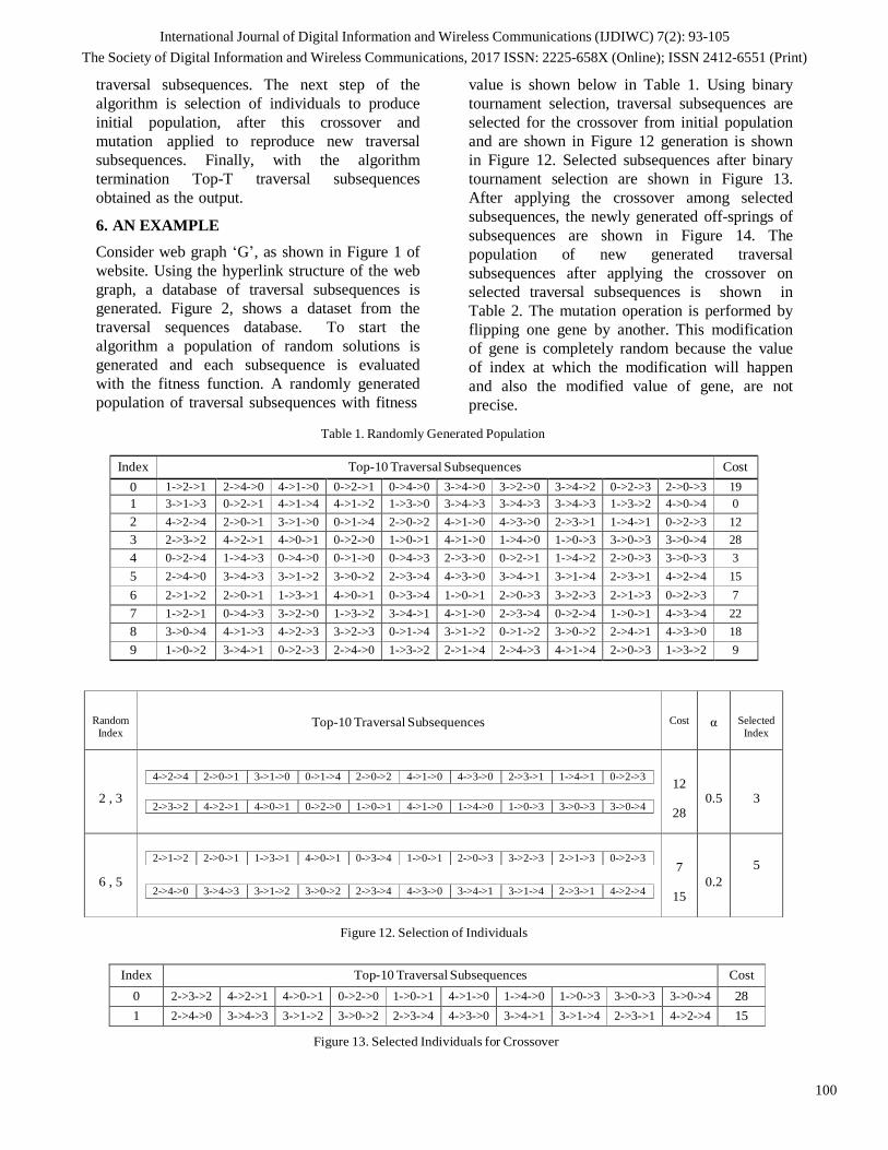
International Journal of Digital Information and Wireless Communications (IJDIWC) 7(2): 93-105
The Society of Digital Information and Wireless Communications, 2017 ISSN: 2225-658X (Online); ISSN 2412-6551 (Print)
100
4->2->4 2->0->1 3->1->0 0->1->4 2->0->2 4->1->0 4->3->0 2->3->1 1->4->1 0->2->3
2->3->2 4->2->1 4->0->1 0->2->0 1->0->1 4->1->0 1->4->0 1->0->3 3->0->3 3->0->4
2->1->2 2->0->1 1->3->1 4->0->1 0->3->4 1->0->1 2->0->3 3->2->3 2->1->3 0->2->3
2->4->0 3->4->3 3->1->2 3->0->2 2->3->4 4->3->0 3->4->1 3->1->4 2->3->1 4->2->4
traversal subsequences. The next step of the
algorithm is selection of individuals to produce
initial population, after this crossover and
mutation applied to reproduce new traversal
subsequences. Finally, with the algorithm
termination Top-T traversal subsequences
obtained as the output.
6. AN EXAMPLE
Consider web graph „G‟, as shown in Figure 1 of
website. Using the hyperlink structure of the web
graph, a database of traversal subsequences is
generated. Figure 2, shows a dataset from the
traversal sequences database. To start the
algorithm a population of random solutions is
generated and each subsequence is evaluated
with the fitness function. A randomly generated
population of traversal subsequences with fitness
value is shown below in Table 1. Using binary
tournament selection, traversal subsequences are
selected for the crossover from initial population
and are shown in Figure 12 generation is shown
in Figure 12. Selected subsequences after binary
tournament selection are shown in Figure 13.
After applying the crossover among selected
subsequences, the newly generated off-springs of
subsequences are shown in Figure 14. The
population of new generated traversal
subsequences after applying the crossover on
selected traversal subsequences is shown in
Table 2. The mutation operation is performed by
flipping one gene by another. This modification
of gene is completely random because the value
of index at which the modification will happen
and also the modified value of gene, are not
precise.
Table 1. Randomly Generated Population
Index Top-10 Traversal Subsequences Cost
0 1->2->1 2->4->0 4->1->0 0->2->1 0->4->0 3->4->0 3->2->0 3->4->2 0->2->3 2->0->3 19 1 3->1->3 0->2->1 4->1->4 4->1->2 1->3->0 3->4->3 3->4->3 3->4->3 1->3->2 4->0->4 0 2 4->2->4 2->0->1 3->1->0 0->1->4 2->0->2 4->1->0 4->3->0 2->3->1 1->4->1 0->2->3 12 3 2->3->2 4->2->1 4->0->1 0->2->0 1->0->1 4->1->0 1->4->0 1->0->3 3->0->3 3->0->4 28 4 0->2->4 1->4->3 0->4->0 0->1->0 0->4->3 2->3->0 0->2->1 1->4->2 2->0->3 3->0->3 3 5 2->4->0 3->4->3 3->1->2 3->0->2 2->3->4 4->3->0 3->4->1 3->1->4 2->3->1 4->2->4 15 6 2->1->2 2->0->1 1->3->1 4->0->1 0->3->4 1->0->1 2->0->3 3->2->3 2->1->3 0->2->3 7 7 1->2->1 0->4->3 3->2->0 1->3->2 3->4->1 4->1->0 2->3->4 0->2->4 1->0->1 4->3->4 22 8 3->0->4 4->1->3 4->2->3 3->2->3 0->1->4 3->1->2 0->1->2 3->0->2 2->4->1 4->3->0 18 9 1->0->2 3->4->1 0->2->3 2->4->0 1->3->2 2->1->4 2->4->3 4->1->4 2->0->3 1->3->2 9
Random
Index
Top-10 Traversal Subsequences
Cost
α
Selected
Index
2 , 3
12
28
0.5
3
6 , 5
7
15
0.2
5
Figure 12. Selection of Individuals
Index Top-10 Traversal Subsequences Cost
0 2->3->2 4->2->1 4->0->1 0->2->0 1->0->1 4->1->0 1->4->0 1->0->3 3->0->3 3->0->4 28 1 2->4->0 3->4->3 3->1->2 3->0->2 2->3->4 4->3->0 3->4->1 3->1->4 2->3->1 4->2->4 15
Figure 13. Selected Individuals for Crossover

International Journal of Digital Information and Wireless Communications (IJDIWC) 7(2): 93-105
The Society of Digital Information and Wireless Communications, 2017 ISSN: 2225-658X (Online); ISSN 2412-6551 (Print)
101
Parent_Ttraversal_Subsequence 1
crossover point
2->3->2 4->2->1 4->0->1 0->2->0 1->0->1 4->1->0 1->4->0 1->0->3 3->0->3 3->0->4
2->4->0 3->4->3 3->1->2 3->0->2 2->3->4 4->3->0 3->4->1 3->1->4 2->3->1 4->2->4
Parent_Ttraversal_Subsequence 2
Crossover
New_Traversal_Subsequence 1
2->4->0 3->4->3 3->1->2 3->0->2 2->3->4 4->1->0 1->4->0 1->0->3 3->0->3 3->0->4
New_Traversal_Subsequence 2
2->3->2 4->2->1 4->0->1 0->2->0 1->0->1 4->3->0 3->4->1 3->1->4 2->3->1 4->2->4
Figure 14. Crossover between Two Individuals
Table 2. Top-10 Traversal Subsequence after Crossover
Index Top-10 Traversal Subsequences Cost
0 2->3->2 4->2->1 4->0->1 0->2->0 1->0->1 4->3->0 3->4->1 3->1->4 2->3->1 4->2->4 6 1 2->4->0 3->4->3 3->1->2 3->0->2 2->3->4 4->1->0 1->4->0 1->0->3 3->0->3 3->0->4 37 2 2->3->2 4->2->1 4->0->1 0->2->0 1->0->1 4->3->0 3->4->1 3->1->4 2->3->1 4->2->4 6 3 2->4->0 3->4->3 3->1->2 3->0->2 2->3->4 4->1->0 1->4->0 1->0->3 3->0->3 3->0->4 37 4 2->3->2 4->2->1 4->0->1 0->2->0 1->0->1 4->3->0 3->4->1 3->1->4 2->3->1 4->2->4 6 5 2->4->0 3->4->3 3->1->2 3->0->2 2->3->4 4->1->0 1->4->0 1->0->3 3->0->3 3->0->4 37 6 2->3->2 4->2->1 4->0->1 0->2->0 1->0->1 4->1->0 1->4->0 1->0->3 3->0->3 3->0->4 28 7 3->0->4 4->1->3 4->2->3 3->2->3 0->1->4 3->1->2 0->1->2 3->0->2 2->4->1 4->3->0 18 8 2->1->2 2->0->1 1->3->1 4->0->1 0->3->4 1->0->1 2->0->3 3->2->3 2->1->3 0->2->3 7 9 2->4->0 3->4->3 3->1->2 3->0->2 2->3->4 4->3->0 3->4->1 3->1->4 2->3->1 4->2->4 15
Here in Figure 15, the value of gene at index 3 is changed from (0->2->0) to (0->1->2) where the
2->3->2 4->2->1 4->0->1 0->2->0 1->0->1 4->3->0 3->4->1 3->1->4 2->3->1 4->2->4 Mutation Index
2->3->2 4->2->1 4->0->1 0->1->2 1->0->1 4->3->0 3->4->1 3->1->4 2->3->1 4->2->4
Figure 15. Mutation Operation
Table 3. Top-10 Traversal Subsequence after Mutation
Index Top-10 Traversal Subsequences Cost
0 2->3->2 4->2->1 4->0->1 0->2->0 1->0->1 4->3->0 3->4->1 3->1->4 2->3->1 4->2->4 6 1 2->4->0 3->4->3 3->1->2 3->0->2 2->3->4 4->1->0 1->4->0 1->0->3 3->0->3 3->0->4 37 2 2->3->2 4->2->1 4->0->1 0->1->0 1->0->1 4->3->0 3->4->1 3->1->4 2->3->1 4->2->4 6 3 2->4->0 3->4->3 3->1->2 3->0->2 2->3->4 4->1->0 1->4->0 1->0->3 3->0->3 3->0->4 37 4 2->3->2 4->2->1 4->0->1 0->2->0 1->0->1 4->3->0 3->4->1 3->1->4 2->3->1 4->2->4 6 5 2->4->0 3->4->3 3->1->2 3->0->2 2->3->4 4->1->0 1->4->0 1->0->3 3->0->3 3->0->4 37 6 2->3->2 4->2->1 4->0->1 0->2->0 1->0->1 4->1->0 1->4->0 1->0->3 3->0->3 3->0->4 28 7 3->0->4 4->1->3 4->2->3 3->2->3 0->1->4 3->1->2 0->1->2 3->0->2 2->4->1 4->3->0 18 8 2->1->2 2->0->1 1->3->1 4->0->1 0->3->4 1->0->1 2->0->3 3->2->3 2->1->3 0->2->3 7 9 2->4->0 3->4->3 3->1->2 3->0->2 2->3->4 4->3->0 3->4->1 3->1->4 2->3->1 4->2->4 15

International Journal of Digital Information and Wireless Communications (IJDIWC) 7(2): 93-105
The Society of Digital Information and Wireless Communications, 2017 ISSN: 2225-658X (Online); ISSN 2412-6551 (Print)
102
Table 4. Top-10 Traversal Subsequence after Generation 2
Index Top-10 Traversal Subsequences Cost
0 2->3->2 4->2->1 4->0->1 0->2->0 1->0->1 4->1->0 1->4->0 1->0->3 3->0->3 3->0->4 28 1 2->3->2 4->2->1 4->0->1 0->2->0 1->0->1 4->3->0 3->4->1 3->1->4 2->3->1 4->2->4 6 2 2->4->0 3->4->3 3->1->2 3->0->2 2->3->4 4->1->0 1->4->0 1->0->3 3->0->3 3->0->4 37 3 2->4->0 3->4->3 3->1->2 3->0->2 2->3->4 4->1->0 1->4->0 1->0->3 3->0->3 3->0->4 37 4 2->3->2 4->2->1 4->0->1 0->2->0 1->0->1 2->3->1 3->4->1 3->1->4 2->3->1 4->2->4 6 5 2->3->2 4->2->1 4->0->1 0->2->0 1->0->1 4->1->0 1->4->0 1->0->3 3->0->3 3->0->4 28 6 2->4->0 3->4->3 3->1->2 3->0->2 2->3->4 4->1->0 1->4->0 1->0->3 3->0->3 3->0->4 37 7 2->3->2 4->2->1 4->0->1 0->2->0 1->0->1 4->3->0 3->4->1 3->1->4 2->3->1 4->2->4 6 8 2->1->2 2->0->1 1->3->1 4->0->1 0->3->4 1->0->1 2->0->3 3->2->3 2->1->3 0->2->3 7 9 2->3->2 4->2->1 4->0->1 0->2->0 1->0->1 4->3->0 3->4->1 3->1->4 2->3->1 4->2->4 6
index value and gene value is randomly chosen. The population of Top-10 traversal subsequences
after generation 1 is shown in Table 3. This becomes the new population for next generation.
After generation 2, Top-10 traversal
subsequences are shown in Table 4.
5, i.e. Top-10 web traversal subsequences after
execution of algorithm: Each subsequence (gene)
in Top-10 traversal subsequences can be used to
reorganize the website structure. The length of
subsequence and number of Top traversal
subsequences can be chosen based on the need
Table 5. Top-10 Traversal Subsequence after Generation 20
Index Top-10 Traversal Subsequences Cost
0 2->4->0 3->4->3 3->1->2 3->0->2 2->3->4 4->1->0 1->4->0 1->0->3 3->0->3 3->0->4 37 1 2->4->0 3->4->3 3->1->2 3->0->2 2->3->4 4->1->0 1->4->0 1->0->3 3->0->3 3->0->4 37 2 2->4->0 3->4->3 3->1->2 3->0->2 2->3->4 4->1->0 1->4->0 1->0->3 3->0->3 3->0->4 37 3 2->4->0 3->4->3 3->1->2 3->0->2 2->3->4 4->1->0 1->4->0 1->0->3 3->0->3 3->0->4 37 4 2->4->0 3->4->3 3->1->2 3->0->2 2->3->4 4->1->0 1->4->0 1->0->3 3->0->3 3->0->4 37 5 2->4->0 3->4->3 3->1->2 3->0->2 2->3->4 4->1->0 1->4->0 1->0->3 3->0->3 3->0->4 37 6 2->4->0 3->4->3 3->1->2 3->0->2 2->3->4 4->1->0 1->4->0 1->0->3 3->0->3 3->0->4 37 7 2->4->0 3->4->3 3->1->2 3->0->2 2->3->4 4->1->0 1->4->0 1->0->3 3->0->3 3->0->4 37 8 2->4->0 3->4->3 3->1->2 3->0->2 2->3->4 4->1->0 1->4->0 1->0->3 3->0->3 3->0->4 37 9 2->4->0 3->4->3 3->1->2 3->0->2 2->3->4 4->1->0 1->4->0 1->0->3 3->0->3 3->0->4 37
The procedure is repeated until the algorithm
converges, and final set of Top-10 traversal
subsequences is shown in Table 5.
Because of the size of web graph taken as the
example is small, the algorithm converged
within 20 generations. After convergence of the
algorithm Top-10 traversal subsequences could
be anyone of the traversal subsequences of Table
of the business manager. Figure 16 shows the top-
10 traversal subsequences after the algorithm
convergence.
7. EXPERIMENTATION
The proposed GA based Traversal Pattern
Mining Algorithm (TPGA) and Incremental
Pattern Mining Algorithm (IPMA) were
implemented with JDK 1.6 in a Window 8
Top-10 Traversal Subsequences Cost
2->4->0 3->4->3 3->1->2 3->0->2 2->3->4 4->1->0 1->4->0 1->0->3 3->0->3 3->0->4 37
Figure 16. Top-10 Traversal Subsequences after Algorithm Convergence

International Journal of Digital Information and Wireless Communications (IJDIWC) 7(2): 93-105
The Society of Digital Information and Wireless Communications, 2017 ISSN: 2225-658X (Online); ISSN 2412-6551 (Print)
103
Support
Count TPGA
CR=50% CR=60% CR=70% CR=80% 5 310 192 281 323
10 408 248 463 351 15 522 538 533 379 20 410 376 246 249 25 389 239 242 223
Support
Count TPGA
CR=50% CR=60% CR=70% CR=80% 5 320 245 330 340
10 529 246 390 347 15 493 498 448 494 20 492 223 426 406 25 479 196 351 348
Spport Count vs Cost (CR=80% , MR=0.05% )
400 350 300
Cos
t TPGA
IPM 100
50 0
5 10 15 20 25
Support Count
Cost
Cos
t
Cost
environment. The comparison was carried out on
the TOP-10 traversal subsequences.
Table 6: Cost of TPGA for MR=0.05
Figure 18. Here also It can be observed from the
graphs that the proposed algorithm TPGA selects
better traversal subsequences at crossover rate of
60% and minimum support count of 15 for the
given graph structure. It can also be noted from
the Table 7 that the algorithm TPGA performs
better at Support Count=15 and Crossover
Table 7: Cost of TPGA for MR=0.10
First the proposed algorithm was run for
different crossover rate and support count
keeping mutation rate fixed at 0.05%. It can be
observed from the graphs shown in Figure 17.
that the proposed algorithm TPGA selects better
traversal subsequences at crossover rate of 60%
S up p or t C o un t vs C o st (C R= 5 0 % , MR= 0 .0 5% ) Support Count vs Cost (CR=60% , MR=0.05% )
6 00
5 00
4 00
3 00
2 00
1 00
0
5 10 1 5 20 25
S u pp or t C o un t
T P G A
IP MA
600
500
400
300
200
100
0
5 10 15 20 25
Support Count
TP GA
IP MA
Support Count vs Cost (CR=70%, MR=0.05%)
600
500
400
300
200
TPGA
IPMA
250
200
150
100
0
5 10 15 20 25
Support Count
Figure 17. Suppurt Count vs Cost at MR=0.05%
and minimum support count of 15 for the given
graph structure. It can also be noted from the
Table 6 that the algorithm TPGA performs better
at Support Count=15 and Crossover rate=60%
when Mutation rate=0.05%.
Similar experiments were performed for
mutation rate of 0.10% and results are shown in
rate=60% when Mutation rate=0.10%.
From the Table 6 and Table 7 it can be noted that
the proposed algorithm TPGA performs better
for mutation rate of 0.05%. So, Both the
algorithms have been compared for Minimum
Support Count=15, Crossover Rate=60% and
Mutation rate=0.05%.

International Journal of Digital Information and Wireless Communications (IJDIWC) 7(2): 93-105
The Society of Digital Information and Wireless Communications, 2017 ISSN: 2225-658X (Online); ISSN 2412-6551 (Print)
104
500
400
S upp ort C ount vs C ost ( C R= 7 0% , MR= 0.1 0)
Cost T P G A
IP MA
100
0
5
10 15 20
S upp ort C ount
25
Cost
Cost
Cost
Cost
S pp o rt C ou n t vs C o st (C R= 5 0% , MR= 0 .1 0) S u p p o r t C o u n t vs C o st ( C R= 6 0 % , M R= 0 . 1 0 )
60 0 6 0 0
50 0
40 0
30 0
20 0
10 0
T P G A
IP MA
5 0 0
4 0 0
3 0 0
2 0 0
1 0 0
T P G A
IP MA
0
5 1 0 15 2 0 25
S u p po rt C o un t
0
5 1 0 1 5 2 0 2 5
S u p p o r t C o u n t
S upport C ount vs C ost (C R= 80, MR= 0.10)
600
500
300
200
400
300
200
100
0
5 10 15 20 25
S uppor t C oun t
T P G A
IP MA
Figure 18. Suppurt Count vs Cost at MR=0.10%
500
400
300
200
100
0
Top-T traversal vs
Cost(Gen=100,CR=50%,MR=0.05)
5 6 7 8 9 10
Top-T traversal subsequences
TPGA
IPMA
structure, thereby presenting the needed and
important information to the user in a few clicks
The comparison of proposed GA based
Algorithm TPGA with IPMA algorithm, shows
that TPGA algorithm performs better as it
produces Top-T traversal subsequences with the
better cost than the cost of Top-T traversal
subsequences produced by IPMA algorithm.
REFERENCES
1. Etzioni, O.: The world wide web: Quagmire or
goldmine. Communications of the ACM, 39(11),
pp.65–68 (1996)
2. Madria, S. K., Bhowmick, S. S., Ng, W. K., Lim, E.-
P.: Research issues in web data mining. In Proceedings of Data Warehousing and Knowledge
Figure 19. Top-T traversal subsequences vs Cost
From the Figure 19, It can be observed that the
proposed TPGA algorithm performs better than
the algorithm IPMA for selecting Top-T
traversal subsequences.
8. CONCLUSION
The proposed GA based algorithm TPGA is used
to find Top-T traversal subsequences from the
traversal patterns. These traversal sequences
could be used to reorganization website
Discovery, First International Conference, DaWaK
‟99, pp 303–312 (1999)
3. Liu, B., Chang, K.: Editorial: Special issue on Web
Content Mining. SIGKDD Explorations,Volume 6,
Issue 2, pp.1-4 (2004)
4. Kosla, R., Blockeel, H.: Web Mining Research: A
Survey. SIGKDD Explorations Vol. 2,pp. 1-15 (2000)
5. Eirinaki, M., Vazirgiannis, M.: Web Mining for web
personalization. ACM Transactions on Internet
Technology (TOIT), 3 (1), pp.1–27 (2003)
6. El-Sayed, M., Ruiz, C., Rundensteiner, E.A.: FS-
Miner: efficient and incremental mining of frequent
sequence patterns in web logs, Proceedings of the 6th
annual ACM international workshop on Web

International Journal of Digital Information and Wireless Communications (IJDIWC) 7(2): 93-105
The Society of Digital Information and Wireless Communications, 2017 ISSN: 2225-658X (Online); ISSN 2412-6551 (Print)
105
information and data management, Washington DC,
USA, November 12-13(2004)
7. Yen, S.J.: An efficient approach for analyzing user
behaviors in a web-based training environment, Int. J.
Dist. Edu. Technol. 1 (4) 55–71(2003)
8. Lee, Y.S., Yen, S.J., Tu, G.H., Hsieh, M.C.: Web
usage mining: Integrating path traversal patterns and
association rules, in: Proceedings of International
Conference on Informatics, Cybernetics, and Systems,
pp. 1464–1469(2003)
9. Lee, Y.S., Yen, S.J., Tu, G.H., Hsieh, M.C.: Mining
traveling and purchasing behaviors of customers in
electronic commerce environment, in: Proceedings of
IEEE International Conference on e-Technology, e-
Commerce and e-Service, pp. 227–230(2004)
10. Lee, Y.S., Yen, S.J.: Incremental and Interactive
Mining of Web Traversal Patterns. Information
Sciences, vol. 178, pp. 287-306 (2008)
11. Agrawal, R., Srikant, R.: Mining Sequential Patterns.
Proceedings of the Eleventh International Conference
on Data Engineering, p.3-14, March 06-10 (1995)
12. Chen, M.S., Huang, X.M., Lin, I.Y.,: Capturing user
access patterns in the web for data mining. in:
Proceedings of IEEE International Conference on
Tools with Artificial Intelligence, pp. 345–348(1999)
13. Chen, M.S., Park, J.S., Yu, P.S.: Efficient data mining
for path traversal patterns in a web environment. IEEE
Trans. Knowl. Data Eng. 10 (2) 209–221(1998)
14. Pei, J., Han, J., Mortazavi-Asl, B., Zhu, H., Mining
access patterns efficiently from web logs. in:
Proceedings of Pacific-Asia Conference on
Knowledge Discovery and Data Mining, pp. 396–
407(2000)
15. Yen, S.J., Lee, Y.S., Cho, C.W.: Efficient approach
for the maintenance of path traversal patterns. in:
Proceedings of IEEE International Conference on e-
Technology, e-Commerce and e-Service, 207–214
(2004)
16. Parthasarathy, S., Zaki, M.J., Ogihara, M.,
Dwarkadas, S.: Incremental and interactive sequence
mining. Proceedings of the eighth international
conference on Information and knowledge
management, Kansas City, Missouri, USA p.251-258,
November 02-06 (1999)
17. Jiadong, R., Zhang, X., Peng, H.: MFTPM: Maximum
frequent traversal pattern mining with bidirectional
constraints, J. Comput. Sci 2(9), pp. 704-709 (2006)
18. Fu, Y., Creado, M., Ju, C.: Reorganizing web sites
based on user access patterns, in: Proceedings of the
Tenth International Conference on Information and
Knowledge Management, ACM Press, pp. 583–585
(2001)
19. Borges, J., Levene, M.: Data mining of user
navigation patterns. In Proceedings of the
WEBKDD‟99 Workshop on Web Usage Analysis and
User Profiling, pp. 31–36 (1999)
20. Kumar, R., Raghavan, P., Rajagopalan, S., Sivakumar,
D., Tompkins, A., Upfal, E.: The Web as a graph. In
Proceedings of the nineteenth ACM SIGMOD-
SIGACT-SIGART symposium on Principles of
database systems, ACM, pp. 1-10(2000)
21. Miller, B.L., Goldberg, D.E.,: Genetic algorithms,
tournament selection, and the effects of noise.
Complex Systems, 9(3), pp.193-212(1995)
22. Maier, D.,: The Complexity of Some Problems on
Subsequences and Super Sequences, J. ACM,ACM
Press, 25(2), pp.322-336(1978)
23. Goldberg, D.E,: Genetic Algorithms in Search,
Optimization, and Machine Learning. Addison-
Wesley(1989)

106
International Journal of Digital Information and Wireless Communications (IJDIWC) 7(2): 106-117
The Society of Digital Information and Wireless Communications, 2017 ISSN: 2225-658X (Online); ISSN 2412-6551 (Print)
Development of Electronic Document Archive Management System (EDAMS): A Case
Study of a University Registrar in the Philippines
Las Johansen B. Caluza
Leyte Normal University
ABSTRACT
The traditional method of data storage has
shown its impact in managing documents
from security, retrieval, and monitoring.
Many kinds of literature suggest that this
approach would result in low job satisfaction
rating from its clients. Leyte Normal
University‟s Office of the Registrar is no
escape in this dilemma. In November 2013,
the university experienced the strongest
typhoon ever recorded known as Haiyan
locally known as Yolanda. The
archive/storage area of the Registrar was
heavily affected were most of the documents
scattered and deteriorated. With this
experience, it is empirical to study to
provide a practical solution. The researcher
utilized embedded single case study using
thematic analysis in identifying the issues
and coping strategies of the seven
participants through in-depth interviews,
focus group discussion, and observation.
Moreover, the utilization of Systems
Development Life Cycle‟s Sashimi model in
developing the software was carried out.
The result revealed various issues and
coping strategies mentioned by the
participants, from a limited storage area to
difficulty in document retrieval and
monitoring, and from the utilization of
logbook to misclassification of records.
Finally, the results became the basis for
developing the electronic document archive
and management system (EDAMS).
KEYWORDS: software development,
qualitative-case study, systems development
life cycle, Philippines.
1. INTRODUCTION
Information systems have shown its
significant impact and importance in the
digital age. A study reveals the benefits of
having a digitmiesal process were fast and
increased productivity, better monitoring,
high level of accuracy, and high level of
consistency of information [1]. Many
organizations are developing information
systems designed specifically to facilitate
the sharing and integration of knowledge
[2]. Despite the application of technologies,
there are still using the manual process of
data storage and retrieval which hinders the
productivity, efficiency, and accuracy of
information and the quality service itself [3]
identified four (4) problems in traditional
methods of data storage such as it takes too
long to acquire, it costs too much regarding
maintenance, it is not scalable enough, and it
requires too much commitment. The use of
the manual process of data storage and
traditional methods of data storage still exist
in the university. As observed, many
students transact the University Registrar
every day, which the Staff needs to attend
this diverse client and request. The tendency
of data filing, retrieval, and releasing of
documents will be affected due to the
current set-up and processes they are
dealing. These gaps identified by the

107
International Journal of Digital Information and Wireless Communications (IJDIWC) 7(2): 106-117
The Society of Digital Information and Wireless Communications, 2017 ISSN: 2225-658X (Online); ISSN 2412-6551 (Print)
literature and through observation are the
primary concern of this study.
2. FRAMEWORK
Build automation theory is the act
of scripting or automating a wide variety of
tasks. Build automation includes managing
the pre and post compile and link activities.
There are many advantages in building
automation systems. Among those were
improved product quality, accelerate the
compile and link processing, eliminate
redundant tasks, minimize "bad builds,"
eliminate dependence on the main
personnel. Also, have a history of builds and
releases to investigate issues, Save time and
money - because of the reasons listed above.
In Agile software development, having a
computerized system or using
working software allows us to measure how
fast we produce results. Which in this case,
the theory would like to imply regarding
acceleration of the process, eliminating
redundant task, and save time and money in
general.
A systematic process through process
transformation from manual to computerize
is now the trends and keeps on moving
forward. The use of Systems Development
Life Cycle (SDLC) in developing systems
plays a vital role in information processing.
This theory was once compared the then and
now by Computer World and the article says
“Software development consisted of a
programmer writing code to solve a problem
or automate a procedure. Nowadays,
systems are so big and complex that teams
of architects, analysts, programmers, testers
and users must work together to create the
millions of lines of custom-written code that
drive our enterprises [4]” In developing
Information Systems (IS) using SDLC are
the most appropriate methodology and the
most commonly used for systems
development analysis and design effort [5].
In support of the SDLC theory in developing
systems Samanga Amarasinghe [6] stated
that “Software development is the process
whereby one creates a set of instructions that
directs a computer to perform a given task(s)
in a particular order, using specified
hardware devices, memory allocation, and
others.” SDLC has different types of models
which software developers can choose from
based on its usefulness and appropriateness
of the kind and purpose of the system to be
developed. Some of these were the Iterative
model, Waterfall model, Sashimi model,
Spiral model, Fish Bone or Ishikawa
Diagram, and Prototyping. In Software
Engineering, it is a part of an approach
called Software Requirement Analysis
(SRA). This SRA presents the requirement
gathering process that intensifies and
focused specifically on software. In this
method, to further understand the nature of
the software or program(s) to be developed,
the researcher or software engineer must
understand the information domain for the
software, as well as required function,
behavior, performance, and interface [7].
The theory mentioned serves as a vital
benchmark towards the development of the
system.
3. THE STUDY
This study utilized embedded single-case
study design using thematic analysis
approach. Wherein the main instrument was
an interview conducted by the researcher,
including narratives of the participants about
the current situation in the workplace. As a
faculty of Information Technology and

108
International Journal of Digital Information and Wireless Communications (IJDIWC) 7(2): 106-117
The Society of Digital Information and Wireless Communications, 2017 ISSN: 2225-658X (Online); ISSN 2412-6551 (Print)
Computer Education unit of the Leyte
Normal University and the interest in
systems development and web engineering
area, the researcher observed in the daily
transactions in the registrar office, the
researcher became interested in creating a
system that the Registrar will benefit from
and the university itself regarding quality
service.
This study would like to investigate
the process of document retrieval and record
keeping of the paper archives of the Leyte
Normal University Registrar. Moreover, the
researcher would like to develop a digital
document archive of all pertinent student
documents that were not found or included
in the current Integrated School Information
System (ISIS).
Specifically, this study would like to
seek the following questions:
1. What are the issues faced by the
office of the university registrar
in dealing with documents
received from the students,
monitoring, and retrieval?
2. How do they cope up with these
issues?
3. Based on the results of this study,
what System can be developed to
solve their problem in data
management, monitoring, and
retrieval?
En route to resolve the current
dilemma found in the university registrar
office, the researcher was requested by the
university registrar to create a system that
will handle and listen to the workload of its
personnel. This study utilized embedded
single-case study using thematic analysis. In
the development of the system, the
researcher used the fusion of Iterative and
Waterfall Method in Systems Development
Life Cycle (SDLC). A Lifecycle covers all
the stages of software from its inception
with requirements definition through to
fielding and maintenance [8]. The use of
process model in SDLC is a practice by
which systems developers use and follows
before, during and after the development of
a system which will become a product called
software. With this project development, the
researcher uses the Sashimi model originated
by Peter DeGrace and an additional
feedback mechanism of Waterfall model.
Determine
Design and
Testing
Implementat
Maintenance
Figure 1: Sashimi and Waterfall Model
Waterfall model in software development
methodologies is one of the most widely
known and recognized methodologies. It
suits for projects where the requirements are
clear. Using the Waterfall software
development life cycle, the implementation
of the system preceded by requirements
definition, analysis, design and development
[9]. The researcher uses this method because
the system will continuously improve for
further enhancement of other transactions
into the system. In effect, a system for the
university registrar will be developed and
utilized.
3.1 Determine Requirements and Analysis

109
International Journal of Digital Information and Wireless Communications (IJDIWC) 7(2): 106-117
The Society of Digital Information and Wireless Communications, 2017 ISSN: 2225-658X (Online); ISSN 2412-6551 (Print)
This study was conducted at the Leyte
Normal University specifically the retrieval
of student request of pertinent records that
were not included in the ISIS like document
retrieval such as Transcript of Records
(TOR), Diploma, Form 137, Form 138,
Honorable Dismissal, Good Moral, Birth
Certificate (NSO), Marriage Certificate
(NSO), Certificate of Transfer Credentials,
Informative Copy of Transcript, Original
Copy of TOR. Currently the university
registrar process around an average of three
hundred (300) request per day, whether the
information found in the ISIS or the Student
Archives. This enormous number of
transactions per day will affect the service of
the university registrar. In effect, a request
of a particular clientele would take time due
to this reason.
Quantitative design using the descriptive
method and qualitative design was utilized
by the researcher to determine the detailed
responses of the respondents towards the
processes and transactions in the University
Registrar‟s Office, and a narrative response
from the respondents was also conducted to
gather more information. A survey
questionnaire was used as its primary
instrument and supported by interview and
observation to fill in other ambiguous
processes, transactions, and questions.
3.2 Design and Coding
In this phase of the spiral model, the
researcher starts the development of the
software using software engineering best
practices such as planning, requirements,
and analysis, change control, quality control,
progress and maintenance, and support after
delivery of the product [10]. To facilitate the
requirements of the system, the researcher
uses programming languages such as
hypertext pre-processor (PHP) programming
as the main computer programming
languages for web development system.
PHP programming was created by Rasmus
Lendorf and was commonly known before
as Personal Home Page and continuously
improved by rewriting its parser by Zeev
Suraski and Andi Gutmans and later
introduce to Zend scripting to deliver higher
performance and supported by running
under the web servers like Apache as a
native server module [1e]. Other scripting
languages where JavaScript to facilitate the
data manipulation before its processing in
the server-side scripting of the system. The
use of HTML5, which is the latest version of
the Hyper Text Markup Language (HTML)
for web development document creation and
the use of Cascading Style Sheet version 3
(CSS3) as the latest version in web
designing. To enhance more the design and
system prototype the researcher uses Twitter
Bootstrap created Mark Otto and Jacob to
facilitate the look-and-feel of a system in
web engineering. A bootstrap is an open-
source JavaScript Framework set up by the
team at Twitter. It is a combination of
JavaScript, HTML5, and CSS3 to give an
easy creation of web design and
functionalities of a website [12]. Through
the use of these latest software development
programming languages and scripting
languages, the development of systems will
be easy, manageable, and fast.
3.3 Testing
Since the researcher uses the sashimi model
and obvious improvements to the waterfall
and other models in SDLC is during the

110
International Journal of Digital Information and Wireless Communications (IJDIWC) 7(2): 106-117
The Society of Digital Information and Wireless Communications, 2017 ISSN: 2225-658X (Online); ISSN 2412-6551 (Print)
testing phase of the project. Testing occurs
as part of the development proves and then
again in the context of the deployment
process. There are several different types of
testing; the researcher uses the following:
System testing, Functional testing,
Performance testing, Loading testing, and
Compatibility testing [9].
3.3.1 Function Testing
Modules, subprograms, and other
related system functionalities were
tested by the researcher/developer to
understand the risk part of the
program further and be able to
respond necessary action or solution
to the problem identified by the
researcher and the registrar‟s
personnel.
3.3.2 Performance Testing
In this phase, the researcher does
some trial and observation of the
actual system performance during
Loading and Compatibility Testing.
In which, observation in real time
processing in this phase was
performed.
3.3.3 Load Testing
This testing phase includes actual
document sample scanning and
feeding information to the system.
The researcher observed how the
system behaves during and after
information attachment and data
storage or saving to the system.
3.3.4 Compatibility Testing
Compatibility issues were
undertaken by the researcher by
checking the hardware components
such as scanners that will be used for
document scanning to produce
electronic copy, server computer to
serve as the controller of the system
to avoid possible computer hacking
and virus attack. However, it is
limited to network username and
password regarding system‟s
protection. The client side computer
is also tested to understand the
behavior further and its compatibility
regarding data processing.
3.3.5 System Testing
The actual system testing and
determining the quality of clean data,
time processing, and overall
performance of the developed system
was performed in this phase. To be
able to accomplish this phase the
researcher together with a
representative of the office of the
University Registrar conducted and
followed software engineering
techniques and approaches in testing
and quality assurance by passing
several testing phases mentioned
above such as Function,
Performance, Loading, and
Compatibility Testing.
3.4 Implementation
After the software quality testing, transfer of
technology will follow, wherein technology
transfer agreement is carried out between the
researcher/developer of the software and
research and the implementing agency (the
university). R.A. 10055 also known as the

111
International Journal of Digital Information and Wireless Communications (IJDIWC) 7(2): 106-117
The Society of Digital Information and Wireless Communications, 2017 ISSN: 2225-658X (Online); ISSN 2412-6551 (Print)
“Philippine Technology Transfer Act of
2009” [13] says:
An act providing the framework and
support system for the ownership,
management, use, and
commercialization of intellectual
property generated from research
and development funded by
government and for other purposes.
It is this premise that the technology
developed by the research had to transfer to
the university as a result of its
investigations, being one (1) of the core
functions of a government employee in the
education sector. Moreover, a proposal to
conduct and transfer of technology by the
researcher and the implementing agency or
its sub-office (the Registrar) of the
university. The University, upon accepting
the said developed software, a memorandum
of agreement (MOA) will be arranged and
be signed by both parties. Technology
Transfer Arrangement refers to conventions
or agreements. Technology transfer includes
renewals thereof, including the transfer of
systematic knowledge for the manufacture
of a product. It is also the transfer of the
application process, or rendering of a
service, including management contracts;
and the transfer, assignment or licensing of
all forms of intellectual property rights,
including licensing of computer software
except computer software developed for the
mass market [14]. Training will also be done
and will be included in the proposal and will
consider the availability of the researcher
and the end user (registrar personnel). After
which, the installation process will follow.
3.5 Maintenance
Several stages performed in maintaining the
system where some of which were
prerequisites and required knowledge
involved, like PHP programming skills,
networking skills, database management
systems skills, and designing skills.
Troubleshooting of the developed system is
easy provided that the above criteria be
satisfied.
4. RESULTS AND DISCUSSIONS
Theme 1: Issues Faced by the University
Registrar
The issues faced by the University Registrar
showed in figure 2 illustrate through a
qualitative schematic network. One
identified issue was a limited storage area
which due to limited space in the university
and the effect of natural disasters like
typhoon, earthquake, and fire. Recently, the
university experienced the strongest typhoon
ever recorded with international name
“Super Typhoon Haiyan” that destroyed
almost 90% of infrastructures like buildings
in the university resulting to heavy damages
of storage area and the office of the
university registrar.

112
International Journal of Digital Information and Wireless Communications (IJDIWC) 7(2): 106-117
The Society of Digital Information and Wireless Communications, 2017 ISSN: 2225-658X (Online); ISSN 2412-6551 (Print)
Limited space in the
University
Document
Misclassification
Misplacement of
Documents
Difficulty in
document
monitoring
Limited storage
area
Document Security
Natural disaster like
Typhoons,
Earthquake, and
Fire
Termite and Pest
Attack
Document
Degradation
Difficulty in
Document
Retrieval
Figure 2: Schematic Network of Issues
Faced by the University Registrar
According to the Staff of the University
Registrar during the interview, “Most of the
documents in the storage area were wet and
disarranged due to strong winds and heavy
rain. Some of the documents were blown
away that causes to misclassification and
degradation of records.” Having a limited
storage area causes document
misclassification, misplacement of
documents, document security is at stake,
termite and pest attack, and document
degradation. The following causes
mentioned above would result in difficulty in
the document monitoring, difficulty in
document retrieval, and contrariwise. These
issues give dilemmas to the Office
considering that the records they are keeping
are student‟s records and other pertinent
information about the students that in the
future these documents will be requested by
the stakeholder.
Theme 2: Coping Strategies of the
University Registrar
Coping strategies identified and mentioned
during the interview and observation with
the participants was established. Among
those coping strategies were asking support
from the administration through the budget
allocation of requests through Annual
Procurement Plan (APP) of the University.
Through APP, the office was able to apply
for maintenance technologies and
infrastructure. As mentioned by the
participant, she said: “The University always
has strong support to the office through
APP, where all requests were given like air
con, shelves, glass separator and protector,
individual enveloped filing and a lot more.”
However, the release of these requests also
takes time. That hinders the efficiency of the
office, with this situation that office resorted
to using Log book of all documents received
and released to the stakeholder. Using the
log book as attested by the participants
would result in improper filing and would
take time of releasing documents.

113
International Journal of Digital Information and Wireless Communications (IJDIWC) 7(2): 106-117
The Society of Digital Information and Wireless Communications, 2017 ISSN: 2225-658X (Online); ISSN 2412-6551 (Print)
Figure 4: Login Form
Admin support
through Budget
Take time in
releasing
Maintenance
Technologies and
Infrastructure
Log Book
Improper filing
Periodic
maintenance (clean-
up, checking)
Underman Take time in
releasing documents
Figure 3: Schematic Network of Coping
Strategies of the University Registrar
Further, despite this budget support, the
office is still lacking Staff to help them
manage stakeholder‟s request, especially
that the University is getting bigger in
student population both in the
Undergraduate and Graduate Students.
According to the participant “We are
under man, we lack Staffs in the office to
help us in managing the Office, that is
why we have periodic maintenance in the
storage area and rotational assignment
as to who will be assigned in cleaning
and checking the documents in the
storage area.” Being under-staffing
would result in inefficiency and
unsatisfactory performance of the office
and would affect the service quality
render to the stakeholders like graduates,
parents, the students itself, and others
transacting the office.
Developed Software
Figure 4 shows the Login form of the
system. This form is the primary security
mechanism of the system against
intrusion or unauthorized user.
Figure 5: Adding New Record

114
International Journal of Digital Information and Wireless Communications (IJDIWC) 7(2): 106-117
The Society of Digital Information and Wireless Communications, 2017 ISSN: 2225-658X (Online); ISSN 2412-6551 (Print)
Figure 5 shows adding new record to the
system. This is where the user of the
system input basic information about the
owner of the document received from the
client like NSO Birth Certificate, Form
137, Honorable dismissal, TOR, and
others.
Figure 6 shows searching student‟s records
through Student ID or Family Name also
the result of the search key. This
mechanism is for fast searching and
retrieval of documents of a specific
student or graduate.
Figure 6: Search Result
Figure 7: Searching List Form
Figure 8: Searching List Result Form
Figure 7 shows the searching list form
indicating a specific list of student‟s records
specified by the user by student number
and by year (from – to). This form is
another way of generating reports by a
list of students with submitted pertinent
and required documents of the University
through the Office of the Registrar.
Figure 8 revealed the result from figure 7
showing the search list result from
displaying the result by Graduate or
Undergraduate by Program, Sex, Document
Status, Enrolled as, and a list of the available
year(s) per program.
Figure 9 shows a sample list report
generated from figure 8 by program
showing the Student Number, the name
of the Student, Sex, Document Status
(complete or incomplete), Enrolled as
(regular or irregular), and Enrollment
Status (Active or Inactive). The result
showed in alphabetical order of Family
Name and arranged using pagination.

115
International Journal of Digital Information and Wireless Communications (IJDIWC) 7(2): 106-117
The Society of Digital Information and Wireless Communications, 2017 ISSN: 2225-658X (Online); ISSN 2412-6551 (Print)
Figure 10 is another report generated
from the system showing the sample
Monitoring Form. This form shows
the Student Number, Student‟s Name,
mandatory document status, Optional
documents and status, Monitoring
Remarks, and Status of the Student.
This form helps a lot to the Office
because this is where they will see and
monitor the required documents,
especially when the student is about to
graduate. Through this report, the
Office can easily provide and quick
feedback to the student as to what
documents are still lacking.
Figure 9: Sample List Report Result
Figure 11 shows form in managing the
system also known as the Maintenance
Form where adding new programs,
document type, a list of programs, and
a list of documents currently saved in
the system. Also, this form performs
editing and deleting programs and
documents.
Figure 10: Sample Monitoring Form Generator
Figure 11: Maintenance Form
5.0 CONCLUSION
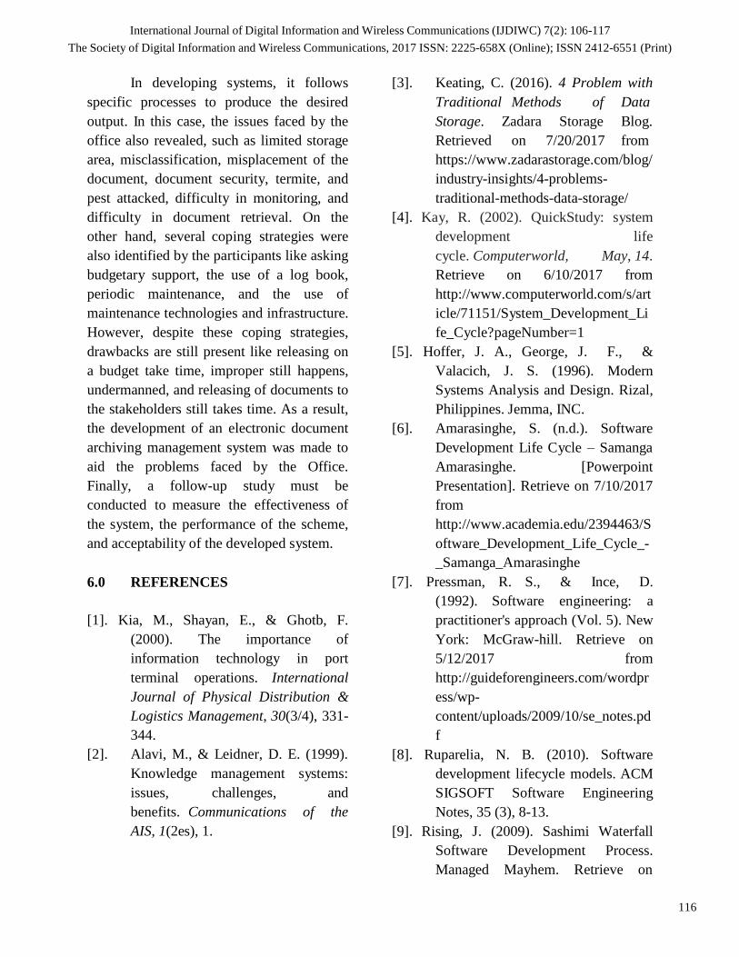
116
International Journal of Digital Information and Wireless Communications (IJDIWC) 7(2): 106-117
The Society of Digital Information and Wireless Communications, 2017 ISSN: 2225-658X (Online); ISSN 2412-6551 (Print)
In developing systems, it follows
specific processes to produce the desired
output. In this case, the issues faced by the
office also revealed, such as limited storage
area, misclassification, misplacement of the
document, document security, termite, and
pest attacked, difficulty in monitoring, and
difficulty in document retrieval. On the
other hand, several coping strategies were
also identified by the participants like asking
budgetary support, the use of a log book,
periodic maintenance, and the use of
maintenance technologies and infrastructure.
However, despite these coping strategies,
drawbacks are still present like releasing on
a budget take time, improper still happens,
undermanned, and releasing of documents to
the stakeholders still takes time. As a result,
the development of an electronic document
archiving management system was made to
aid the problems faced by the Office.
Finally, a follow-up study must be
conducted to measure the effectiveness of
the system, the performance of the scheme,
and acceptability of the developed system.
6.0 REFERENCES
[1]. Kia, M., Shayan, E., & Ghotb, F.
(2000). The importance of
information technology in port
terminal operations. International
Journal of Physical Distribution &
Logistics Management, 30(3/4), 331-
344.
[2]. Alavi, M., & Leidner, D. E. (1999).
Knowledge management systems:
issues, challenges, and
benefits. Communications of the
AIS, 1(2es), 1.
[3]. Keating, C. (2016). 4 Problem with
Traditional Methods of Data
Storage. Zadara Storage Blog.
Retrieved on 7/20/2017 from
https://www.zadarastorage.com/blog/
industry-insights/4-problems-
traditional-methods-data-storage/
[4]. Kay, R. (2002). QuickStudy: system
development life
cycle. Computerworld, May, 14.
Retrieve on 6/10/2017 from
http://www.computerworld.com/s/art
icle/71151/System_Development_Li
fe_Cycle?pageNumber=1
[5]. Hoffer, J. A., George, J. F., &
Valacich, J. S. (1996). Modern
Systems Analysis and Design. Rizal,
Philippines. Jemma, INC.
[6]. Amarasinghe, S. (n.d.). Software
Development Life Cycle – Samanga
Amarasinghe. [Powerpoint
Presentation]. Retrieve on 7/10/2017
from
http://www.academia.edu/2394463/S
oftware_Development_Life_Cycle_-
_Samanga_Amarasinghe
[7]. Pressman, R. S., & Ince, D.
(1992). Software engineering: a
practitioner's approach (Vol. 5). New
York: McGraw-hill. Retrieve on
5/12/2017 from
http://guideforengineers.com/wordpr
ess/wp-
content/uploads/2009/10/se_notes.pd
f
[8]. Ruparelia, N. B. (2010). Software
development lifecycle models. ACM
SIGSOFT Software Engineering
Notes, 35 (3), 8-13.
[9]. Rising, J. (2009). Sashimi Waterfall
Software Development Process.
Managed Mayhem. Retrieve on

117
International Journal of Digital Information and Wireless Communications (IJDIWC) 7(2): 106-117
The Society of Digital Information and Wireless Communications, 2017 ISSN: 2225-658X (Online); ISSN 2412-6551 (Print)
5/10/2017 from
http://www.managedmayhem.com/2 009/05/06/sashimi-
waterfall- software-development-process/
[10]. Jones, C. (2010). Software
Engineering Best Practices: Lessons
from Successful Projects in the Top
Companies. New York. The
McGraw-Hill Companies.
[11]. PHP Manual. (n.d.). A Brief History
of PHP. Retrieve on 9/8/2013 from
http://scholar.lib.vt.edu/manuals/php
3.0.6/intro-history.html
[12]. Markle, B. (2013). What is
Bootstrap?. Support Center. Retrieve
on 6/9/2017 from
http://www.inmotionhosting.com/su
pport/edu/joomla-3/using-
bootstrap/what-is-bootstrap
[13]. Republic Act. 10055 of 2009.
Retrieved on 5/15/2017 from
public_acts/ra%2010055.pdf
[14]. IPOPHIL. (nd). About Technology
Transfer Agreement. Retrieved on
6/16/2017 from
http://www.ipophil.gov.ph/index.php
/services/ip-business2/technology-
transfer-arrangement

118
International Journal of Digital Information and Wireless Communications (IJDIWC) 7(2): 118-123
The Society of Digital Information and Wireless Communications, 2017 ISSN: 2225-658X (Online); ISSN 2412-6551 (Print) of 6.
Data Mining and Analysis for off Grid Solar PV Power System
Mohamed D. Almadhoun
Department of IT, University College of Applied Sciences
Gaza, Palestine
ABSTRACT
Solar power generation systems production changes with
respect to geographical location. By this paper we
studied how solar systems behave in Gaza which is
located in the Middle East. Log readings of off grid solar
PV power supply system included PV module, array
combiner, off grid inverter, battery and load. Data
entered many techniques of data mining to discover the
hidden and meaningful patterns, and to analyze results.
Classification was applied to discover rules which can
help in supporting solar power system functionality of
alerting about expected power generation and needed
costs. Association rules were applied to find
relationships between variables and plot events of power
changing. Clustering were used to categorize power
production values and study properties of each.
The scope of study extended to discover effects of solar
and moon months, input voltage and charging current,
daytime hours, daytime temperatures, and effects of week days on power generation.
Resulting knowledge were novel, actionable,
understandable, and valid. This was stated by tracking
the confidence rates and applying evaluation by cross
validation.
KEYWORDS
Renewable energy, Solar systems, PV power generation,
data mining, Knowledge Discovery in Database.
1 INTRODUCTION
Data mining is an approach to extract patterns from
large data sets and deduce knowledge insights from
patterns [1]. Data mining can find unsuspected
relationships and summarize the data in novel ways
that are both understandable and useful to the data
owner [2].
Photovoltaic (PV) is a method of generating
electrical power by converting solar radiation into
direct current electricity using semiconductors that
exhibit the photovoltaic effect. PV power
generation employs solar panels composed of a
number of solar cells containing a photovoltaic
material. Manufacturing of solar cells and
photovoltaic arrays has advanced considerably in
recent years because of growing demand for
renewable energy sources [3].
Operating costs for the electricity system may
increase because of the unpredictability of the sun
and unexpected variations of a PV output which
leads to potential threats to the reliability of
electricity supply. Predicting changes is a main
concern to schedule the reserve capacity and to
administer the grid operations [4]. PV power is
affected by the weather and other natural factors
dramatically. To reduce the energy dissipation and
maintain the security of power grid we should give
priority to predicting PV energy accurately [3].
In the last years data mining and related
applications were used in predicting solar radiation
and solar energy system design to give an overview
of such predictive data mining techniques [5]. Due
to the strong increase of solar power generation, the
predictions of incoming solar energy are too
important and necessary to predict the amount of
energy which will be produced, up to 72 h before,
and deviations of energy production are strongly
penalized [5][6].
In this study data mining is used to find
relationships and rules, and the development trends
of PV solar power generation management systems
[7][5].
This paper follows the process of knowledge
discovery with all steps starting from data
gathering, followed by data cleaning, and
aggregation to make data ready to be utilized for
data visualization and data mining, reaching to the
evaluation and knowledge representation. Data
mining phase will be shown in details and
knowledge represented from each data mining
model.
Three data mining models used: first was
classification by decision tree, second was

119
International Journal of Digital Information and Wireless Communications (IJDIWC) 7(2): 118-123
The Society of Digital Information and Wireless Communications, 2017 ISSN: 2225-658X (Online); ISSN 2412-6551 (Print) of 6.
association rules by FP-Growth approach, and
finally clustering by k-Means approach.
2 RELATED WORKS
Qazi et. al. [5] proposed an overview of predictive
data mining techniques and highlighted the
importance of solar energy systems in terms of
clean environment. Their paper concluded that
ANN-based prediction offers greater accuracy, and
hence it‟s much more dependable and demanding in
the domain of renewable energy resource
predication. Their study demonstrated that ANN
models predict solar radiation more accurately than
statistical, conventional, linear, nonlinear and fuzzy
logic models. As a future work they aim to carry out
in depth research on acceptance of solar systems in
Malaysia.
Hossain et. al. [4] presented an architectural
framework for the construction of hybrid intelligent
predictor for solar power. Their research
investigated the applicability of heterogeneous
regression algorithms for 6 hour ahead solar power
availability forecasting using historical data from
Rockhampton, Australia. Real life solar radiation
data was collected across six years with hourly
resolution from 2005 to 2010. They observed that
the hybrid prediction method is suitable for a
reliable smart grid energy management. Prediction
reliability of the proposed hybrid prediction method
was carried out in terms of prediction error
performance based on statistical and graphical
methods. The experimental results show that the
proposed hybrid method achieved acceptable
prediction accuracy.
Wang et. al. [3] proposed a big data system (Solar
Photovoltaic Power Forecasting System, called
SPPFS) to calculate and predict the power under
real-time conditions. In their system, they utilized
the distributed mixed database to speed up the rate
of collecting, storing and analysis the
meteorological data. In order to improve the
accuracy of power prediction, the given neural
network algorithm has been imported into SPPFS.
By adopting abundant experiments, they show that
the framework can provide higher forecast
accuracy-error rate less than 15% and obtain low
latency of computing by deploying the mixed
distributed database architecture for solar-generated
electricity.
3 DATA MINING FOR UCAS SOLAR
ENERGY SYSTM
A. Data resource
Dataset was created by EAST solar inverter of
model GF6000. This system is equipped in the
University College of Applied Science (UCAS)
which is located in Gaza via Palestine; Dataset is
for device readings for 18 months, with 276,657
instances.
Dataset elements are numerous, general like Date
time, AC input voltage, AC output voltage, AC
output frequency, load level, temperature, PV input
voltage, PV charging current, battery voltage,
battery capacity level, PV power, daily generated
energy, and total generated energy. Some of these
elements were not used in data mining techniques
because they are not related to input/output
operations. In addition, four new attributes where
calculated and extracted from date/time field, first
of them was the period of solar month (such as Jan,
Feb, or Dec), second was period of moon month
(lunar month such, includes months such as
Muḥarram, Safar, or Ramadan), third was week
day, and fourth was time hour period.
B. Data mining process and tasks
Figure 1 lists data mining process steps. First phase
of data mining process was business understanding
of how PV solar system works and what benefits of
this system to UCAS. This information was gotten
from specialists in the computer center department
in UCAS.
Second phase data understanding achieved by
collecting information about each data element,
understanding what these values mean and what are
effects of it.
By the aid of MS excel and rapidminer software
third phase data preparation started. MS Excel
operations helped in generating new attributes from
date/time field. Solar month period was the first
which includes one of three values: 1, 2, or 3, value
of 1 means that this record was added in a date
between 1 and 10 in solar month. Second was Moon
month period which includes values of 1,2, or 3,
and this was calculated on basis of Hijri calendar.
Thirdly, week day was calculated. and finally time
period number which implements day time hours,
that means if value of time period num attribute was

120
International Journal of Digital Information and Wireless Communications (IJDIWC) 7(2): 118-123
The Society of Digital Information and Wireless Communications, 2017 ISSN: 2225-658X (Online); ISSN 2412-6551 (Print) of 6.
10 then this reading sample was added to database
between 10 AM to 11 AM.
After then on rapid miner processes, interesting
elements were selected (Temperature, PV input
voltage, PV charging current, PV power, solar
month, moon month, time period number, and week
day). Instances with PV power value of zero value
were filtered out, so number of instances became
125,765. Because of lots of values and to make
value meaningful, discretize by binning was applied
to each of PVInputVoltage, PVPower, and
Temprature with number of bins equals five.
Fourth phase modeling was applied through three
different tasks, each of which informs about
different knowledge. They were applied using
rapidminer software.
First task was classification using decision tree
technique which is a tree-structured plan of a set of
attributes having several possible alternative
branches of values in order to predict the class label.
Classification can be useful in the field of PV power
generation systems in expecting how much power
can be generated in case we have some information
about atmosphere and calendar. It also can give us
an indication on quantities of fuel needed to power
generation station in case of cities that use hybrid
power sources. Figure 2 shows a branch of resulting
decision tree.
Decision tree model was rich of knowledge, pruning
was used to get rid of useless branches to avoid
overfitting. Its criterion was information gain, and
maximal depth of 4. In case of selecting attributes:
moon month period, solar month period,
temperature, PVpower (class label), and
PVChargingCurrent, some knowledge inferred from
decision tree was such as: most range values of
PVPower matched the same range value of
PVChargingCurrent attribute which means positive
relationship, solar month period appeared in the tree
but moon month period did not and that means solar
month period has more effect on
PVChargingCurrent than moon, also we find in two
cases that third part of solar month causes a
degradation in generated power despite of high
charging current. Decision tree model algorithm
seeks to build tree with least levels and this depends
on calculating information gain that increases with
the average purity of subsets that an element
produces [8], so PVChargingcurrent attribute was
selected as root element in the tree, and that
confirms that the most affecting input of generated
PV power is PVChargingcurrent.
1- Business Understanding
Understand objectives and requirements from PV power generation perspective
2- Data Understanding
Data collection for device readings, Identify quality problems, Detect interesting subsets
3- Data Preparation
Data cleaning to get rid of incomplete, noisy, or inconsistent data, data selection for relevant data to the analysis task, data transformation into proper formats for
applying data mining model
4- Modeling
Classification, Association rules, and Clustering
5- Evaluation Ensure that model acheives business
objectives
6- Deployment (Knowledge Representation) Organize and present knowledge
Figure 1 Data mining process steps and tasks

121
International Journal of Digital Information and Wireless Communications (IJDIWC) 7(2): 118-123
The Society of Digital Information and Wireless Communications, 2017 ISSN: 2225-658X (Online); ISSN 2412-6551 (Print) of 6.
Figure 2 PVChargingCurrent Decision Tree
In case of selected attributes: moon month period,
solar month period, temperature, PVpower (class
label), and PVInputVoltage, we will get Figure 3
tree in which the PVInputVoltage is the root. 79.3%
of range3 PVInputVoltage samples produced a
PVpower value in range1 which means that voltage
of solar cells current does not ensure high power
like PVChargingCurrent. Moon month has more
effect on PVInputVoltage where it appeared in tree.
Figure 3 PVInputVoltage Decision Tree
Second task of data mining modeling phase was
creating association rules by FP-Growth operator.
This model is used to discover interesting
relationships between disjoint items of dataset.
Items can be defined as different values of
elements. Relationship can be presented in a pattern
of the form x -> y where x and y are item sets [8].
Association rules can be useful in the field of PV
power generation systems by informing about those
relations between elements and give useful
knowledge about changeability relations between
elements as a guidance of how to get more
generated power. Figure 4 shows some resulting
rules by association rules model with their
evaluation factors support, confidence, and lift.
Selected attributes for this model were Moon Month
Period, PVInputVoltage, PVPower, Solar Month
Period, Temperature, Time Period Num, and Week
day.
Association rules were numerous, knowledge were
extracted carefully according to background in that
field and good consideration for data mining factors
which are support, confidence, and lift. So
association rules added that most likely high
produced PVInputVoltage values can be in the time
period between 12:00 and 13:00 in Gaza, despite of
high PVInputVoltage the PVpower values will be
low in case of temperature between 32 and 38, it‟s
more likely to get lower PVpower values when it‟s
a day between 11 and 20 of solar month (solar
month period 2), Wednesday is strongly related to
low PVpower values, and probability of low
PVpower values can increase when a day fall in
solar month period 2 and in moon month period 3 or
a day falls in solar month period 3 and in moon
month period 1.
Figure 4 Some Resulting Rules from Association Rules Model
Figure 5 Resulting Clusters

122
International Journal of Digital Information and Wireless Communications (IJDIWC) 7(2): 118-123
The Society of Digital Information and Wireless Communications, 2017 ISSN: 2225-658X (Online); ISSN 2412-6551 (Print) of 6.
Third task was clustering by k-Means operator. This
model is used to group data instances with similar
characteristics or features together into a separate
cluster [8]. Clustering helps to categorize affecting
situations on generating PV power so this gives an
indication on how to deal with that situation. Figure
5 shows how points are distributed between
clusters.
Clusters were distributed up to their counts as
shown in Figure 6, It‟s obvious that cluster_1 is the
majority (94308 items=75% of samples), and by
studying centroid table of clustering model it was
noticed that the cluster_0 has moderate and high
values of PVpower and PVChargingCurrent, but
cluster_1 has low values of PVpower and
PVChargingCurrent.
Figure 6 Clusters Counts
C. Evaluation
In order to estimate the statistical performance of a
learning operator such as decision tree model, we
use cross validation as an evaluation technique with
ten validations. Cross validation defines a training
set and testing set and runs classification model
many times with changing testing set each time to
reach to an unbiased success rate.
Accuracy of constructed decision tree model was
81.74%, Figure 7 shows performance vector.
Figure 7. Performance Vector of Decision Tree Classification Model
4 CONCLUSION
PV solar power generation management systems
can be exploited well if a good data mining process
was applied on it with the guidance of specialists.
This paper followed all data mining process steps to
produce trusted results.
Main goal of data mining is to announce novel,
actionable, understandable, and valid patterns. By
applying association rules process and decision tree
model a set of novel, actionable, and understandable
knowledge was gotten.
Most important knowledge informed about that
solar month periods affects PV charging current, but
moon month periods affects PV input voltage. In
addition, input voltage coming from solar cells does
not ensure high power but PV charging current
does. Also, highest produced PV input voltage
values can be in the time period between 12:00 and
13:00 in Gaza. Furthermore, high temperatures
produces low PV power values. Mostly PV power
values decreases in the day of Wednesday, but can
increase when day fall in solar month period 2 and
in moon month period 3.
Future work can be considered if another datasets
were available to re-apply models and get more
accurate and actionable patterns, and to consider
months as new attribute given a dataset of many
years. Recommendation to PV management
software developers is to add the functionalities of
alerting about expected PV power generation to
make decision makers take actions in the right way.
REFERENCES 1. M. Kraft, K. Desouza, and I. Androwich, “Data Mining in
Healthcare Information Systems: Case Study of a
Veterans‟ Administration Spinal Cord Injury Population,”
Proceedings of the 36th Hawaii International Conference
on System Sciences, 2002.
2. A. Gosain, and A. Kumar, “Analysis of Health Care Data
Using Different Data Mining Techniques,” Proceedings
of International Conference on Intelligent Agent & Multi-
Agent Systems. IAMA 2009.
3. J. Wang, Y. Chen, R. Hua, P. Wang, and J. Fu, “A
distributed big data storage and data mining framework
for solar-generated electricity quantity forecasting,”
Proceedings of the SPIE, Volume 8333, article id.
83330S, pp. 7, 2011.
4. M. Hossain, A. Oo, and A. Ali, “Hybrid Prediction
Method for Solar Power Using Different Computational
Intelligence Algorithms,” Smart Grid and Renewable
Energy, vol. 4, pp. 76-87, 2013.
5. A. Qazi, H. Fayaz, and R. Raj, “Discourse on Data
Mining Applications to Design Renewable Energy

123
International Journal of Digital Information and Wireless Communications (IJDIWC) 7(2): 118-123
The Society of Digital Information and Wireless Communications, 2017 ISSN: 2225-658X (Online); ISSN 2412-6551 (Print) of 6.
Systems,” Proceedings of International Conference on
Advances in Engineering and Technology (ICAET'2014),
Singapore, March 2014.
6. L. Martín, L. Zarzalejo, J. Polo, A. Navarro, R.
Marchante, and M. Cony, “Prediction of global solar
irradiance based on time series analysis: Application to
solar thermal power plants energy production planning,”
Solar Energy, Volume 84, Issue 10, October 2010, Pages
1772-1781, ISSN 0038-092X.
7. M. Almadhoun and A. El-Halees, “Different Mining
Techniques for Health Care Data Case Study of Urine
Analysis Test,” Proceedings of Fifth International
Conference on Intelligent Computing and Information
Systems (ICICIS), Egypt, 2011.
8. J. Han, and M. Kamber, “Data Mining: Concepts and
Techniques,” the Morgan Kaufmann, 2001.
9. M. Lloyd-Williams, “Case Studies in the Data Mining
Approach to Health Information Analysis,” IEE
Colloquium on Knowledge Discovery and Data Mining
(1998/434), 1998.
International Journal of Digital Information and Wireless Communications (IJDIWC) 7(2): 124-142
The Society of Digital Information and Wireless Communications, 2017 ISSN: 2225-658X (Online); ISSN 2412-6551 (Print)
124
Vulnerability Assessment and Penetration Testing: A proactive approach towards
Network and Information Security Muhammad Zeeshan
1, Shams Un Nisa
2, Tazeen Majeed
3, Nayab Nasir
4, Saadia Anayat
5.
Department of Computer Science and Information Technology
Virtual University of Pakistan, Lahore Pakistan.
Peshawar Campus1, Islamabad Campus
2, Faisalabad Campus
3, 4, Talagang Campus
5.
ms1504005581, ms140400309
2, ms160400234
3, ms150400522
4, ms150401012
ABSTRACT
With increasing dependency on IT
infrastructure, the main objective of a
system administrator is to maintain a
stable and secure network, to identify
common network threats and define
countermeasures to prevent these
threats. The information which is stored
in computer‟s repository may be less
compromised than the information
travelling over the network. Network is
an untrusted environment as compared
to computer‟s repository, so information
needed to kept secret and must not be
stolen. In this paper, we perform an
empirical study on how to do
vulnerability assessment with the aim of
search for any potential loopholes or
vulnerability contain in a system. And
also briefly described the existing tools
of the Pen- testing, no one of the tools
have capabilities to find out all the
vulnerabilities. We will perform
different phases of the penetration
testing for proactively to protect from
any possible treats towards our network.
Hence penetration testers are hoped to
be ethical which conducting tests.
.
KEYWORDS
Vulnerability, DDoS, DNS, Spoofing,
Asset, Capabilities, Privilege
Escalation.
1.INTRODUCTION
Vulnerability assessment is the process
of digging out these black holes and
then reporting along with necessary
measures to overcome these black holes
to avoid any mishap. In this paper we
will through light on basic IT security
concepts along with common network
attacks and vulnerabilities form where
attacks exploit. [1] This repot also
covers penetration testing. What
procedures penetration testing undergo.
Scope of Pen-Test, Pen-Test
Approaches, Models, Techniques etc.
Pen-Test formal and standard report
formats, case study and
countermeasures to cover vulnerabilities
in Pen-Test report are parts of this
report.
This paper is divided into various
sections. In section ii, iii and IV the
author will describes what is
vulnerabilities and why vulnerabilities
Assessment, in section V and VI the
network vulnerabilities and threat to
network vulnerabilities is described.
The section IX to XVII details the
different texts of vulnerabilities like
PEN-Testing, Black Box Testing, White
Box Testing and Gray Box Testing,
XIX is last section where author
conclude this paper with the complete
details of the work of vulnerabilities
Assessment and Penetration Testing.
2. VULNERABILITY
Vulnerability in network security term
that refers to flaw or weakness in the
network or system from where any
attacker can get into our network or
system to exploit. The network or
system having these vulnerabilities is
called vulnerable network or vulnerable
system. More the network system is
vulnerable; more is the threat to exploit.
Millions of systems exploit every year
due to vulnerabilities. Vulnerable
network or system may be
compromised by different attacks like,
DDoS, DNS Spoofing, DHCP
Snooping, ARP Poisoning, Man-in-the-
Middle, Smurf attacks, Buffer overflow,
SQL injection attack and other many
cyber-attacks along with a number of
malicious attacks including Viruses,

International Journal of Digital Information and Wireless Communications (IJDIWC) 7(2): 124-142
The Society of Digital Information and Wireless Communications, 2017 ISSN: 2225-658X (Online); ISSN 2412-6551 (Print)
125
Trojan Horse, Worms, Malwares and
root kits etc. These vulnerabilities
usually result from week passwords,
software bugs, non-patching of
software‟s and operating systems. Script
code injection spaces etc.
3. VULNERABILITY
ASSESSMENT
Vulnerability Assessment (VA) or
Vulnerability Analysis (VA) or
Vulnerabilities Scanning is the process
of defining, identifying and classifying
vulnerabilities in a network or
communication system. This also
includes series of systematic measures
used to review and prioritize security
vulnerabilities in a network or
communication system/ or any
application service. Vulnerability
Assessment assists businesses in the
determination of security posture of the
environment and the level of exposure
to threats.
Figure1: Vulnerability Assessment [2]
Vulnerability Assessment has a superior
role in every type of computer
applications, system and infrastructure.
Any system providing any kind of
computing service may have
vulnerabilities so VA test is very much
important for every kind of computer
application. In computer networks and
communications, our information use to
travel out of computers so presence of
vulnerabilities may compromise our
whole networks to exploited.
Vulnerability Assessment can be more
effective and valuable if performed in
following order. [2]
Classification of Assets,
Capabilities, and Resources.
Assigning values and significance
of these resources.
Identifying vulnerabilities and
potential threats to each resource.
Mitigating and eliminating most
somber vulnerabilities for the most
important assets, resources and
capabilities. Repeating steps from 1 to 4 in the
same order after prescribed time
frame.
The process of vulnerability assess
should be repeated after fixed
prescribed time intervals (in general
quartile basis). This will help the team
to cover any vulnerability timely that
may occur in a network system. VA can
be as single or the combination on both
automated and manual scan of IT/
network infrastructure and without VA
there is a risk that the network is not
secured which may result serious
exploits.
4. WHY VULNERABILITY
ASSESSMENT?
The main purpose of any organization
to make profits towards its vision and
goals. So organizations have
opportunity to deploy Information
Technology Infrastructures. So securing

International Journal of Digital Information and Wireless Communications (IJDIWC) 7(2): 124-142
The Society of Digital Information and Wireless Communications, 2017 ISSN: 2225-658X (Online); ISSN 2412-6551 (Print)
126
the network and communication system
is the core objective after deployment to
prevent an attacker to get into network
that can be set a very large potential risk
for the system.
Therefore vulnerability assessment
performs to check out black holes in a
system. Objective of Vulnerability
Assessment may include System
Accreditation, Risk Assessment,
Network Auditing, Compliance
Checking and Continuous Monitoring.
These vulnerabilities may occur from
weak passwords, flaws in systems,
faulty and inappropriate configuration
and human errors like, inappropriate
permissions assigned to users,
inappropriate network design and
devices and like this etc. Some business
standards institutions like PCI-DSS
require organizations to perform
vulnerability assessment on their
network or systems.
5. COMMON NETWORK
VULNERABILITIES
Networks and communication
infrastructures are deployed for
information sharing between devices.
So our data or information has to travel
out of devices like computers, tabs and
mobile phones etc. Data and
information have more threat of get
compromised when out of our
computers [3] . Data may travel on
wired or wireless medium.
Vulnerabilities in our networks
welcome attackers to get in
communication systems to exploit. Here
major network vulnerabilities are being
listed from typical reviews.
5.1 Missing patches
Security patches are the software that
system developers provide time to time
after their continuous research on
operating systems or software they
provide to end users. These patches
must be installed on operating systems.
These patches cover any vulnerability in
the system. Not needed all patches but
recommended patches must be installed
on core operating systems like servers
cover related vulnerabilities. For
example installation of security updates
provided by Microsoft may cover
possible vulnerability present in web
server.
5.2 Weak or default
passwords
Many systems like Domain Systems,
Database Systems, Routers, Switches,
Firewalls, IDS/IPS, Web Applications
along with web servers and other
systems like these are configured with
week or default password. These
passwords can easily be guessed and
probed. This scheme must be changed
to keep default password intact. For
example if we purchase a D-Link
Wireless Access Point for our home
usage. It has configured with default
username “admin” and default password
“admin”. Any attacker has easy access
to our wireless network by these
password schemes. So passwords must
be changed to customize and must be
kept complex to guess by any attacker.

International Journal of Digital Information and Wireless Communications (IJDIWC) 7(2): 124-142
The Society of Digital Information and Wireless Communications, 2017 ISSN: 2225-658X (Online); ISSN 2412-6551 (Print)
127
5.3 Miss-configured
firewall rules
Use of firewall in to prevent
unauthorized access is pretty good
practice but most of the times miss-
configuration of rules on firewalls is a
vulnerability. These rules may contain
serious weaknesses that allow
unauthorized access in network
systems. So firewalls should be ruled
according to standards. OWASP has
defined wonderful policies for firewall
configuration as well.
5.4 Mobile devices
Uses of wireless mobile devices like
laptops, tablets, smart phones pose a
greatest risk in our network system to
get hacked. Almost all mobile devices
can store cookies, web passwords,
cache passwords; emails containing
sensitive data in have a big vulnerability
when connecting these devices with
corporate networks.
5.5 USB flash drives
Use of USB devices are a pattern. These
devices may contain passwords and
other sensitive information; if stolen or
misplaced can be a cookbook for an
evildoer. These portable devices may
contain malware and viruses which can
harm our system inside the firewall.
Other vulnerabilities include
authentication bypassing, plaintext
passwords, wireless key enumeration,
privilege escalation, gaining access,
buffer overflow, remote command
execution, cryptographic vulnerabilities
like weak encryption algorithms and
keys etc. These loopholes must be
covered to ensure security.
6. THREATS TO VULNERABLE
NETWORKS
Presence of vulnerabilities may
welcome a vast number of network
threats. These threats include Malware,
Viruses, Worms, Payloads, Trojan
Horses, Spywares, Root kits, Port
Scanning, Social Engineering, MAC
Address Spoofing, DoS and DDoS
attacks, ARP Poisoning Attacks [4].
These threats can also be categorizes as
Untrusted Threats, Structured Threats,
External Threats and Internal Threats
and a vast number of cyber-attacks
other than these. Every attack has its
own potential towards networks. These
attacks can takes place due to presence
of vulnerabilities in network of
telecommunication systems.
7. VULNERABILITY
MANAGEMENT LIFE CYCLE
Vulnerability management is a
continuous rotating process to Discover,
Prioritize Assets, Assessment,
Reporting, Remediating, and to
verification that vulnerabilities have
been eliminated.

International Journal of Digital Information and Wireless Communications (IJDIWC) 7(2): 124-142
The Society of Digital Information and Wireless Communications, 2017 ISSN: 2225-658X (Online); ISSN 2412-6551 (Print)
128
Figure 2: Vulnerabilities Management Life Cycle [4]
These steps have been further elaborated given as under.
7.1 Discover
To record all assets of the network,
operating systems and other devices, list
all vulnerabilities on a regular schedule.
7.2 Prioritize
Categorize assets and assign values to
those assets groups based on their
importance in business operation.
Assess: - To determine a baseline risk
profile based on assets priority, risk and
vulnerabilities.
7.3 Report
Measure the assets according to security policy of business organization.
Document assessment based on security
risks, threats and known vulnerabilities.
7.4 Remediate
Fix vulnerabilities according to business
risks. Enable access controls and cover
loop holes in network systems.
7.5 Verify
Verify that vulnerabilities that were
discovered have eliminated. These may
be carried out by security audits.

International Journal of Digital Information and Wireless Communications (IJDIWC) 7(2): 124-142
The Society of Digital Information and Wireless Communications, 2017 ISSN: 2225-658X (Online); ISSN 2412-6551 (Print)
129
8. PENETRATION TESTING
(PEN-TESTING)
Penetration Testing or simply Pen-
Testing or Security Testing is the
technique refers to the attempt to
discover vulnerabilities in network
system before an attacker exploits. This
is the act of gaining access to networks
or systems resources without the
knowledge of user credentials like
usernames and passwords. Penetration
testing report visualize the evidence that
vulnerabilities are present in your
network or system from there
penetration is possible in. moreover a
penetration test report is capable to
visualize the proactive and remedial
measures to protect your network and
enhance comprehensive defensive
strategy. The penetration test report also
depicts the satisfactory security
approaches adopted by our security
responsible professionals. These test
report are also often required by
security agencies, law-and-order
agencies, information systems auditors
and other stockholders.
It is significant to discuss that it is
unlike that a pen-tester will uncover all
vulnerabilities in one pen-test report.
For example if a pen-tester has
generated a report today it is obvious
that it may no longer be valid after one
month. It is because after the approval
of pen-test report by owner, system may
have get patched with new updates
which may last a vulnerability in some
web server which may considered
secure in last pen-test report. So
maintain a secure infrastructure,
constant vigilance is considered
necessary.
9. PEN-TESTING vs VA
People often consider as Penetration
Testing and Vulnerabilities Assessment
are two names of same term but in
actual these two terminologies have
difference upto some extent.
Vulnerabilities Assessment mainly
covers the scoping of different areas
that are vulnerable to network attacks
whereas Penetration testing mainly
refers to gaining most possible access
inside the vulnerable networks and sets
standards to cover these vulnerabilities
in the network. Vulnerabilities
assessment process stops just before the
system is compromised whereas break
in as far as the scope of the agreement.
Penetration tests are important for a
number of reasons like:-
Determining the possibility of
particular attacks to take place.
Discover high risk vulnerabilities
resulting from low risk
vulnerabilities.
Identifying vulnerabilities that may be
difficult or impossible to detect with
general scanning software.
Identifying magnitude of a successful
attack to a vulnerable network.
Testing capabilities of network
defenders to detect and response to
network attacks.
Provide evidence to increase allocations in security budgets.
Testing a new system before its online
launching is a good practice. By this
practice lots of vulnerabilities are
identified before the system launching

International Journal of Digital Information and Wireless Communications (IJDIWC) 7(2): 124-142
The Society of Digital Information and Wireless Communications, 2017 ISSN: 2225-658X (Online); ISSN 2412-6551 (Print)
130
to avoid serious exploits. The Payment
Card Industry (PCI) Data Security
Standard (DSS) define Penetration
Testing Standards. At least these
standards are required to get meet for
satisfactory pen-testing approach.
Let us consider comparison from
another aspect as in tabular description
Vulnerability Assessment Penetration Testing
Attributes List-oriented Goal-oriented Type of Reports Prioritized list of vulnerabi-lities
categorized by critica-lly for
remediation
Specific information of what data was
compromised and
vulnerabilities exploited Purpose Identify security vulnerab- ilities
in system that may be exploited Determine whether an
application can withstand
an intrus- ion attempt
Table 1: Comparison of Vulnerability Assessment and Penetration Testing [5]
10. WHY PENETRATION
TESTING?
Penetration testing is an essential
practice to ensure that organization‟s
network is secure and upto date in
meeting security standards. So by
escaping to perform penetration test in
systems is attempting to leverage the
vulnerabilities discovered hence there is
no way of knowing the risks that are
presented to network system based on
those vulnerabilities. We may divide
why to perform penetration testing from
different perspectives i.e. Business
Perspective and Operational
Perspective.
10.1 Business Perspective
of Penetration Testing
Penetration testing safeguards IT
systems against failure by preventing
financial losses. Organizations do spend
millions of dollars from information
security breaches on notification costs,
remedial measures after system
compromises for security which further
lead to deceased productivity and lost
revenue. So penetration testing helps in
identification and nominates the risks
before a security breach can occur
which to prevent financial losses due to
security is valuable in breaches to
overcome a huge cost for recovery.
Authenticated industry standards have
mandated as regulatory requirements for
computing security systems, in case
noncompliance heavy fines or other
penalties may be imposed on those
organizations during IT security audit
processes.
Single incident of security breach may
lead organization to loss of customers‟
confidence, challenges in marketing
strategies, dishonor of other
stockholders and even failure of entire
business. The study of CSI has

International Journal of Digital Information and Wireless Communications (IJDIWC) 7(2): 124-142
The Society of Digital Information and Wireless Communications, 2017 ISSN: 2225-658X (Online); ISSN 2412-6551 (Print)
131
estimated that the recovery may costs
approximates upto $167700.00 per
incident which is very huge amount.
Penetration Testing assesses value of
existing security products and provides
the supporting opinion of future
investment in information technology
security mechanisms. PT can provide an
evidence of issue and solid proposal of
investment in IT security.
10.2 Operation
Perspective of
Penetration Testing
Penetration testing helps shape up
security procedures through appropriate
vulnerabilities identification and
assessment procedures. This help out
proactive elimination of threats and
risks, corrective and preventive
measures, quickly real potential
vulnerabilities. Penetration testing can
help to fine tune or patch to proactively
eradicate the risks that have been
identified during the process of
vulnerabilities assessment.
11. WHO TO PERFORM
PENETRATION TEST?
PCI DSS does not entail that QSA or
ASV to execute a penetration test. PCI
DSS requires performing this test by
either expert internal resource or expert
third party. If internal resources are to
perform this test then these
professionals must be well equipped
and well qualified. Usually these
professional are separate from the
system for which penetration testing is
being performed. For example a
network administrator should not be
engaged to perform penetration test of
his own domain. Same case for other
network domains like firewall, domain
services or web services. Beside of
these, at least following capabilities
make comparatively good penetration
testing professional.
Mysterious understanding
with Operating systems.
Expert in
networking technologies including
OSI, TCP/IP,
DHCP, DNS, Routing, Switching,
Snooping, ARP/RARP, STP/RSTP,
all network security threats and
attacks and all other areas which are
not discussable here.
Deep understanding
with scripting, BAT or VB Scripting.
Low lever
programming techniques
including assembly languages,
system programming and
network level programming.
Deep understanding with cores
or network firewalls and proxy
servers. Access control using these
resources. After mastering these
basics, one can move to PIX or ASA
firewalls.
Vast working with IPS and IDS.
How to use these devices to prevent
our networks and what are
dimensions of these devices. Knowledge of computer forensic domain.
Must be database expert and
at home in handling all complex
level
problems in Database Management Systems and System Analysis.
12. PENETRATION TESTING
TYPES

International Journal of Digital Information and Wireless Communications (IJDIWC) 7(2): 124-142
The Society of Digital Information and Wireless Communications, 2017 ISSN: 2225-658X (Online); ISSN 2412-6551 (Print)
132
Two main types of Pen-Testing are
Physical Penetration Testing and
Virtual Penetration testing. Physical
includes tangible assets like Data
Centers, Servers, Routers, Switches,
CCTV Systems, Security Barriers and
Security Guards etc. in this type
penetration testers use to assess security
loop holes that may exists in accessing
IT gadgets physically. No unauthorized
personals have access to these gadgets
like Data Centers, Equipment and
infrastructure. So a comprehensive
policy is needed to be defined regarding
physical assets. Other natural disaster
proofing falls also in physical
penetration testing. It is needed to
outcome that our building where core
network infrastructure exists must be
proofed in case flood, earthquake,
heavy rain, storm, fire and even Cooling
of Data Centers Equipment, Humidity
etc.
Virtual penetration testing refers to
testing virtual assets or intangible assets
include Operating Systems, Software‟s,
Web Servers, IOS, Firewalls, Databases
and other intangible assets in a business
organization. Most of network attacks
take place due to vulnerabilities in
virtual infrastructures. These attacks are
often software lever attacks which
include, DoS/DDoS, Spoofing, DHCP
Snooping, ARP Poisoning, Database
Injection, phishing, overflows, exploit,
password and hijack attacks etc.
penetration testing and vulnerabilities
assessment in virtual assets is more
challenging that for physical assets.
More than 80% energies are expended
in protecting these virtual assets as
compared protecting physical assets.
Besides these penetration testing types
it is pertinent to closely classify
penetration testing in another manner.
Penetration testing i.e. Physical PT,
Network PT and Social Engineering PT.
Network Penetration testing is an
ethical way of the identification of
security flaws of networks. Test is
applied on network devices like
modems, switches, routers, remote
access devices, IPS/IDS, Firewalls and
other devices in network to scan the
network.
On the other hand, application
penetration testing scans an
application‟s security controls by
highlighting risks posed from potential
vulnerabilities in applications. Many
organizations use firewalls and other
traffic monitoring systems to protect
information whereas security threats
still exist due to a number of hidden
vulnerabilities which is needed to be
explored and system should be
protected.
Social Engineering is another very
important field that imposes security
threats to organizations. Social
Engineering involves human interaction
to compromise information about
computer system of an organization. So
Social Engineering Penetration Testing
process determines the level of security
awareness among workers that directly
and indirectly own IT systems of the
organization. Social Engineering
penetration test also observes that upto
what extent an organization‟s workers
can exploit organization‟s secrets that
are harmful for existing system.

International Journal of Digital Information and Wireless Communications (IJDIWC) 7(2): 124-142
The Society of Digital Information and Wireless Communications, 2017 ISSN: 2225-658X (Online); ISSN 2412-6551 (Print)
133
13. PEN-TESTING
METHODOLOGIES
There are three known strategies of
penetration testing that profession
testers use to adopt. These
methodologies include Black Box,
White Box and Gray Box Penetration
Testing.
13.1 Black Box Testing In Black Box Testing, the testers do not have any knowledge about target. They
have to dig out vulnerabilities and
loopholes on the basis of their own
scuff. This strategy is similar to blind
test and like procedures adopted by real
attacker who has no idea and
information regarding the
organization‟s network.
13.2 White Box Testing
In white box penetration testing
approach, testers are equipped with all
necessary information about the target.
Generally test team and organization‟s
team work together to perform this kind
of test where all information provided to
the team prior of running test. This
information may include paths,
credentials, procedures, addresses and
protocols etc. that are being used in
organization‟s network.
13.3 Gray Box Testing
Gray box testing falls between black
and white box testing in which partial
disclosure of information about test
targets are provided to test teams.
Usually testers does not provided all
information for the target however they
need to gather further information
required by their own before conducting
the test.
Where, there penetration testing
strategies are being discussed, it is
necessary not to ignore two important
penetration testing strategies that are
Internal and External Penetration
Testing.
13.4 External
penetration testing
Techniques involve tests on the target
using procedures performed from
outside of the organization. External
Penetration testing is performed to dig
out possibilities of external hacker can
get in and how far he can be able to gain
access to organization‟s internal
structure.
13.5 Internal penetration testing
Is performed from inside the
organization‟s network that own test
target. This strategy is useful to check
out upto what extent a disgruntled
employee can cause the damage to the
organization. Internal penetration
testing checks out the potential of
harmfulness if organization‟s network successfully penetrated by an authorized
inside user with assigned privileges.
14 AREAS OF
PENETRATION TESTING
Penetration Testing can be performed in
almost areas of information technology.
As the whole IT revolves around data
and information of the business. So data

International Journal of Digital Information and Wireless Communications (IJDIWC) 7(2): 124-142
The Society of Digital Information and Wireless Communications, 2017 ISSN: 2225-658X (Online); ISSN 2412-6551 (Print)
134
at every stage in every area is not
perfectly safe. However major
Penetration Test areas have discussed as
under.
Physical Penetration Testing
Software Penetration Testing
Database Penetration
Testing Network Penetration
Testing Web Penetration
Testing
Wireless Network Penetration
Testing
Social Engineering Penetration
Testing
Cloud Penetration Testing
Operating Systems Penetration
Testing
Mobile Devices Penetration
Testing
This research has scoped to Network
Penetration Testing. Network
Penetration Testing is a critical task and
is very common among all areas of
Information Technology.
15 PHASES OF
PENETRATION
TESTING
There is no hard and fast rule of
conducting penetration testing with
respect to phases of conducting
penetration test however common
phases that every tester must have to go
through are 1. Reconnaissance, 2.
Execution, 3. Discovery. These three steps are baseline of each penetration
test however these phases are further
divided into sub phases for convenience
of penetration testers. I recommend
seven phases of a professional
penetration testing on a target network.

International Journal of Digital Information and Wireless Communications (IJDIWC) 7(2): 124-142
The Society of Digital Information and Wireless Communications, 2017 ISSN: 2225-658X (Online); ISSN 2412-6551 (Print)
135
15.1 Planning
Figure 3: Phases of Penetration Testing [6]
target network deals with this phase.
Information as much as possible are
Planning phase encircles to scope of the test. What are the business objectives
that will be achieved after testing, What
to test, how to test, what conditions will
be applied, the time frame for test
execution and usually cost of the test
are considered in planning phase of
penetration test.
15.2 Reconnaissance
Once the scope of the test has been
defined, the next step is reconnaissance
phase. Information gathering about
gathered in this phase. This is a
comprehensive phase that may include
indentifying target network status,
operating systems, IP addresses range,
open ports, domain name, DNS, DHCP,
Wifi Key, Mail Server Records etc.
Host Finger Printing, Port Scanning, Network Mapping, Network
Enumeration are usually considered in
reconnaissance phase.
15.3 Exploration

International Journal of Digital Information and Wireless Communications (IJDIWC) 7(2): 124-142
The Society of Digital Information and Wireless Communications, 2017 ISSN: 2225-658X (Online); ISSN 2412-6551 (Print)
136
This phase deals with exploring the
entire network based on necessary
information gathered in reconnaissance
phase. More specific to the network
services. Like checked opened ports in
last step. Using opened ports, the tester
enters the network and explore the
network more deeply. Testers scans the
network for discovering network
devices, firewall rules, users accounts
and access control etc. Exploration
include host exploration, services
identification and platform
identification etc.
15.4 Vulnerability Assessment
Finding the existing vulnerabilities by
using both manual and automated
techniques, vulnerability management,
vulnerabilities discovery, threat
classification and values of active and
passive threats to a vulnerable system
are discovered in this phase [7].
Penetration testers may use automated
tools for known vulnerabilities. These
tools are helpful by having updated
databases for latest vulnerabilities and
their details.
15.5 Exploitation
This is more challenging phase in
penetration testing which deals with
attacks to the target network. The
penetration tester tries to exploits for
different vulnerabilities discovered in
last phase. Privilege Escalation in
considered sub part of exploitation
phase in which usually attacker takes
advantage of programming bugs or
design loopholes to crawl to the
privileged access that are usually
protected general users and
applications. The system having more
privileged accounts can be exploits up
to more extent.
15.6 Reporting and
Recommendation
This almost last phase in which testing
team document all of its observations.
This is final document on which all the
phases based. The true and final
purpose of a penetration test is to point
out all vulnerabilities in a network or a
system that have covered in last phases.
Final report should cover all phases‟
activities including a cover sheet,
executive summary of vulnerabilities
found in the network, threats imposed
from these vulnerabilities, list of tools
used and most important final
recommendation after overall
examination of test report. Upon final
recommendation covered in the report,
values of threats and mitigation of
threats are discussed. Final
recommendation phase must be
performed with highly qualified
professionals in which preventive
proposals are provided against founded
vulnerabilities.
16 PENETRATION TESTING
STANDARDS
Following is the list of professional
standards and certifications regarding
penetration testing. These organizations
are well known and are accredited
throughout the Information Security
World.

International Journal of Digital Information and Wireless Communications (IJDIWC) 7(2): 124-142
The Society of Digital Information and Wireless Communications, 2017 ISSN: 2225-658X (Online); ISSN 2412-6551 (Print)
137
EC-Council LPT (Licensed
Penetration Tester)
OSTTMM(Open Source Security
Testing Methodology Manual)
PTF (Penetration Testing
Framework) OWASP(Open Web Application Security Project)
ISSAF (Information Systems
Security Assessment Framework) WASC-TC(Web Application
Security Consortium Threat
Classification)
OISSG (Information Systems Security Assessment Framework)
PCI DSS v3.1 (Payment Card
Industry Data Security Standard)
ISO/IEC27001:2005(Information
Security Management Systems)
ISO/IEC 27005:2008 (Information
Security Risk Management)
17 PENETRATION
TESTING TOOLS
Although there are a vast number of
tools that are used in penetration testing,
however a few most widely using tools
are being discussed in brief. Different
tools are popular to perform different
kind of tasks in different domains. No
single tool is capable to do all tasks in
penetration testing. A combination
among these tools leads to a successful
penetration testing report. Different
flavors of Linux have designed
specifically for Network / Information
Security Assessment however Back
Track 5.0 and Kali Linux have
specifically designed and developed for
this purpose. These are bootable
operating systems that include lots of
tools. Some tools are given as under.
17.1 Nmap
Nmap (Network Mapper) is known as
the World's best port scanner. It is free
tool available in both Back Track and
Kali Linux. It enables testers to perform
network discovery, port scanning, host
discovery, version detection, OS
detection etc. Nmap is usually deployed
in security audit of a device or a
firewall, identification of open ports in
target system, network mapping,
network inventory, asset management
and maintenance, gathering traffic in the
network, finding and exploiting
vulnerabilities in the network. Nmap
uses raw IP packets to find out what
hosts are available, what kind of
services are being offered by those
hosts, what operating systems and their
versions are running on hosts, what kind
of firewalls are installed as well as a
number of other parameters. It is
capable to run on all major operating
systems in both GUI and Command
Line utility. Nmap has a number of
variations like Zenmap, Ncat, Ndiff and
Nping for different tasks associated to
each.
17.2 Nessus
Nessus is top rated network
vulnerability scanner. It was initially
free and open source software designed
to run only on Linux OS however, later
on from 2008, it available with cost and
can run on MAC OS, Windows OS,
Free-BSD platforms. It is so powerful
scanner as its developers conducted a
survey in 2006 of used by almost 75000
organizations. It is web tool that can

International Journal of Digital Information and Wireless Communications (IJDIWC) 7(2): 124-142
The Society of Digital Information and Wireless Communications, 2017 ISSN: 2225-658X (Online); ISSN 2412-6551 (Print)
138
scan vulnerabilities like, vulnerabilities
that allow remote hacker to access
sensitive data, miss configured system
like missing patches, default
passwords, common password
configured, missed passwords etc.
Nessus also powerful in determining
DoS attacks and conducting of PC-DSS
audits etc.
17.3 Metasploit Framework
Metasploit Framework is a power
exploitation tool which enables
penetration tester to develop and
execute exploit code against target
network. It can also be employed to test
vulnerabilities in network system. It is
open source and available free of cost
for almost all versions of UNIX and
Windows. Metasploit Framework
provides attack payloads, attack
libraries that can be put jointly for
modular approach. Main purpose of
Metasploit Framework is to get access
to command prompt of computer in
targeted network. Once command
prompt is accessed it is very easy for
even hacker to have all controls over
that target. Once; from hacker‟s point of
view; the system is accessed, he can
execute code for easier access to target
next time.
17.4 Wireshark
Wireshark is another excellent and
unique tool based on its specific use and
nature. This is another multi platform,
open source network platform analyzer
which scans live data travelling in
network. Wireshark has a number of
dominant features including viewing of
TCP streams in the network. Wireshark
supports a vast variety of protocols and
media types.
17.5 Aircrack
Aircrack is a tool for wireless cracking.
It intelligently can crack 802.11 a/n/g
wireless networks. It uses best wireless
cracking algorithms to recover WiFi
Keys by examining even encrypted
packets. Aircrack has a number of tools
like Airodump, Aireplay, Aircrack-ng
and Airdecap for different assignments.
17.6 Cain & Abel
It is well know UNIX based free
network sniffing tool. This is known
windows only password recovery tool.
It recovers password by network
sniffing, cracking encrypted password
by dictionary attacks, bruit-f0rce
attacks, sniffing VOIP communications,
decoding scrambled passwords,
uncovering cached passwords alongwith
analysis of routing protocols being used
in the network in well documented
manner.
I thing pertinent to at least name other
very important network penetration
testing tools like Snort, NetCat,
TCPDump, John the Ripper, Kismet,
OpenSSH/PuTTY, Brup Suit, Nikto,
Hping, Ettercap, Sysinternals, W3af,
OpenVAS, Scapy, THC Hydra, Paros
Proxy, NetStumbler, WinDump,
Network Security Toolkit, OWASP
Mantra etc. Each tool among these has
specific usage in specific scenario and is
being widely used in penetration testing
and hacking procedures.

International Journal of Digital Information and Wireless Communications (IJDIWC) 7(2): 124-142
The Society of Digital Information and Wireless Communications, 2017 ISSN: 2225-658X (Online); ISSN 2412-6551 (Print)
139
18 ETHICAL
AND LEGAL
ISSUES
However Penetration Testing is the
process of exploring vulnerabilities in a
network in order to find out all
possibilities and loopholes from where
attackers get into the network system
and exploits. In actual Penetration
Testing totally resembles the process of
hacking into networks but only the
difference is that hacking is a crime that
is done illegally whereas penetration
testing is conducted in a legal way.
Different countries have settled codes of
laws for hackers. The owner the
network employee pen-testers to dig out
all the possible holes in order to
mitigate hacking attacks. It is very
pertinent for both parties to sign mutual
agreement before observing a
penetration test. The agreement may
have following clauses [8].
18.1 Written Permission
Pen-Testers must have sign legal
written document duly signed by both
parties prior of conducting s penetration
test. Testers should have to document all of the processes of penetration test.
This will protect testers from any legal
issue in future.
18.2 Damage Control
In some live environments the pen-test
may set a potential harm to the network.
So the testers must have to notify
customer about potential harm or
incidental damage that may occur
during the test. Testers do not take
liability in case incidental harm of
record or deletion of data etc.
18.3 Scope of Work
Pen-Testers must have to define scope
of work defining external and/or
internal vulnerabilities assessment.
Scope also includes which networks,
what systems, what devices will be
performed test on.
18.4 Professional Approach
The pen-testers must have to define that
they will follow well know professional
standard to perform the test even any
vulnerability could not be found. [9]
Also priory defines what kind of service
is needed by the owner like just port
scanning or exploitation etc. It is not
good to make promises of digging hills.
18.5 Premises and Jurisdiction
Jurisdiction of the test should be
defined which clearly depicts the venue
where test is going to be performed.
Different countries may have different
Cyber Laws so performing test in
America may be a legal issue that in
Germany.
18.6 Privacy Issue
A successful pen-test can be performed
by getting into one's computer or
network system. So sensitive data or
databases may be accessed during test
process. So clause of data privacy must
be included in the agreement.
Besides all above cited clauses are in
favor of penetration testers, pen-testers
International Journal of Digital Information and Wireless Communications (IJDIWC) 7(2): 124-142
The Society of Digital Information and Wireless Communications, 2017 ISSN: 2225-658X (Online); ISSN 2412-6551 (Print)
140
are also expected to be ethical during
and after a successful pen-test. Usually,
computer users are not technical and
they rely on the technical professionals
so penetration testers are also needed to
act as doctor not a thief. Because of this,
information and network security is
being monitored and governed by
authorized organizations that have
provided licenses and certifications that
guarantee technical competency along-
with ethical considerations of licensees.
19 CONCLUSION
Penetration testing and vulnerabilities
assessment is a very growing field in IT
security. We perform penetration testing
for proactively protect from any
possible treats towards our network.
Missing patched, weak or default
passwords, opened unnecessary ports,
miss configured firewalls and other
networking devices, mobile and USB
devices are common vulnerabilities, so
penetration testing first points out these
vulnerabilities then provides solutions
to cover these vulnerabilities.
Penetration testing can be performed
externally and internally among three
types as Black Box, White Box and
Gray Box in a number of defined phases
includes Planning, Reconnaissance,
Exploration, Vulnerabilities
Assessment, Exploitation, Reporting
and Recommendation. There are
several tools to conduct a penetration
test like Nessus, Nmap, Metasploit and
Cain & Abel etc. Each tool has
expertise in specific area like Nmap is
best in port scanning and Metasploit is
best in exploitation etc. Penetration
testing is similar in sense of hacking
process hence penetration testing is
legal while hacking is illegal.
Penetration testing is observed upon the
demand of owner whereas hacking is
getting in networks illegally and is a
crime. Hence penetration testers are
hoped to be ethical which conducting
tests.
References
[1 P. Engebretson, The Basics of Hacking and
] Penetration Testing, 225 Wyman Street,
Waltham, MA 02451, USA: Elsevier Inc, 2011.
[2 W. Link,
] "http://en.wikipedia.org/wiki/Vulnerability_a
ssessment".
[3 W. Link, "https://www.offensive-
] security.com/".
[4 J. Benetti, Step By Step Kali Linux and
] Wireless Hacking Basics, 2015 Edition, 2015.
[5 N. F. A. A. M. S. Zainudin, "A Survey on
] Conducting Vulnerability Assessment in Web-
Based Application," in International
Conference on Advanced Machine Learning
Technologies and Applications, Switzerland,
2014.
[6 W. Link,
] "http://www.rhinosecuritylabs.com".
[7 K. K. K. Ankita Gupta, "Vulnerability
] Assessment and Penetration Testing,"
International Journal of Engineering Trends
and Technology, vol. 4, no. 3, pp. 328-333,
2013.

International Journal of Digital Information and Wireless Communications (IJDIWC) 7(2): 124-142
The Society of Digital Information and Wireless Communications, 2017 ISSN: 2225-658X (Online); ISSN 2412-6551 (Print)
141
[8 H. T. Tavani, "Ethics And Technology: Ethical
] Issues In An Age Of Information And
Communication Technology," ACM SIGCAS
Computers and Society, vol. 33, no. 3,
September 2003.
[9 C. N. Sushilkumar Yadav, "Survey: Secured
] Techniques for Vulnerability Assessment and
Penetration Testing," International Journal of
Computer Science and Information
Technologies, vol. 5, no. 4, pp. 5132-5135 ,
2014.
[1 T. G. Proffitt, [2] Creating a Comprehensive
0] Vulnerability Assessment Program for a Large
Company Using Qualys Guard, SANS Institute
Info Sec Reading Room , 2008.
[1 G. Weidman, Penetration Testing: A Hands-
1] On Introduction to Hacking, USA: William
Pollock, 2014.
[1 P. Kim, The Hacker Playbook: Practical Guide
2] To Penetration Testing, North Charleston,
South Carolina: Secure Planet LLC, 2014.
[1 I. John Wiley & Sons, Certified Ethical
3] Hacking Version 8, Indianapolis, Indiana:
Sybax Publishers, 2014.
[1 S. Harris, CISSP All-in-One Exam Guide,
4] Seventh Edition, McGraw-Hill Education,
2016.
[1 White Paper What is a vulnerability
5] assessment?, Miami, Florida, USA: DEMYO
INC, 2011.
[1 E. D. a. C. Easttom, CompTIA Security+ Study
6] Guide: SY0-401, 6th Edition, Sybax
Publishers, 2014.
[1 W. Link,
7] "http://swtestingmatters.blogspot.com/2012
/08/penetration-testing-breaking-in-
before.html".
[1 w. Link,
8] "http://nizarbekai.com/services/penetration-
testing/".
[1 W. Link,
9] "http://www.vulnerabilityassessment.co.uk".
[2 W. Link, "[18]
0] http://www.accuvant.com/blog/strategy-
and-tactics-penetration-testing-in-the-
security-program".
[2 w. Link,
1] "http://www.ibm.com/systems/data/flash/b
e/resources/Attachement_2_-_IBM-ISS-
PenTest-WP060608-073108.pdf".
[2 C. J. N. G. Umesh Kumar Singh,
2] "Measurement of Security Dangers in
University Network," vol. 155, no. 1, 2016.
[2 C. J. N. G. Umesh Kumar Singh, "Information
3] Security Assessment by Quantifying Risk
Level of Network Vulnerabilities," vol. 156,
no. 2, 2016.
[2 V. B. S. a. M. C. Nandi, "Robust and accurate
4] feature selection for humanoid push
recovery and classification: deep learning
approach," 2015.
[2 V. B. S. a. S. K. S. C. Behera, "An optimized
5] feature selection technique based on
incremental feature analysis for bio-metric
gait data classification," 2016.

International Journal of Digital Information and Wireless Communications (IJDIWC) 7(2): 124-142
The Society of Digital Information and Wireless Communications, 2017 ISSN: 2225-658X (Online); ISSN 2412-6551 (Print)
142
Muhammad Zeeshan
received the Master
degree in Computer
Science from Virtual University of Pakistan in
2015. He is currently
working toward the
MSCS degree in
Computer Science at
VUP. His research
interests are Network
Security in cloud
Computing and Attribute Based Access Control. He is currently an employ of FCSC Peshawar,
under Ministry of Defence Islamabad,Pakistan.
Shams Un Nisa is
currently an Lecturer in
the Department of
Computer Science, FG
Degree College Karachi,
SHe received the MCS
and MSCS degree in
Computer Science From
VUP. Her research
interests are cloud and
network security.
Tazeen Majeed is with
Department of Computer
Science & Information Technology as a student
of MSCS at VU, Lahore,
Pakistan. She is
currently working as a
Computer Science
Teacher in Blessing
Home High School, Faisalabad.
Nayab Nasir is with
Department of Computer
Science & Information
Technology as a student
of MSCS at VU, Lahore,
Pakistan. Her research
interests are data mining.
Saadia Anayat is with
Department of Computer
Science & Information
Technology as a student
of MSCS at VU, Lahore,
Pakistan. Her research
interests are data mining,
data warehousing and
cloud computing data
storage.