von trapp rethinking year 15 thesis final
TRANSCRIPT

Rethinking Year 15: What Determines the Terminal Valuation of LIHTC Financed Transactions?
by
Jakob B. von Trapp
B.S., Finance, 2005
Boston College Carroll School of Management
Submitted to the Program in Real Estate Development in Conjunction with the Center for Real Estate
in Partial Fulfillment of the Requirements for the Degree of Master of Science in Real Estate Development
at the
Massachusetts Institute of Technology
September 2013
©2013 Jakob B. von Trapp
All rights reserved
The author hereby grants to MIT permission to reproduce and to distribute publicly paper and electronic copies of this thesis document in whole or in part in any medium now known or hereafter created.
Signature of Author: _____________________________________________________________________________________
Center for Real Estate July 30, 2013
Certified by: _____________________________________________________________________________________
William C. Wheaton Professor of Economics,
Department of Urban Studies and Planning Thesis Supervisor
Accepted by: _____________________________________________________________________________________
David Geltner Chairman, Interdepartmental Degree Program in
Real Estate Development

2
Rethinking Year 15: What Determines the Terminal Valuation of LIHTC Financed Transactions?
by
Jakob B. von Trapp
Submitted to the Program in Real Estate Development in Conjunction with the Center for Real Estate on July 30, 2013 in Partial Fulfillment of the Requirements for the Degree of Master of Science in Real
Estate Development
ABSTRACT The Low Income Housing Tax Credit (LIHTC) program is one of the most successful government subsidy programs for the creation of affordable housing in the history of the United States. Over its 27 year existence, more than two million affordable apartments have been developed or rehabilitated using private equity financing through the sale of federal tax credits. Over the past 12 years the industry has digested the first wave of transactions getting to the end of the 15 year Initial Compliance Period. This is the point at which the Investor Limited Partner (ILP) is able to exit the transaction without tax credit recapture risk with the IRS. There is often a recapitalization event that accompanies the exit, but many times there is not. Since the secondary market for both LP and GP interests both during and after the compliance period is relatively illiquid, it is difficult to discern the fair market value of such an asset. This is further complicated by the unique and multi-‐layered financing structures common in these transactions and the additional 15-‐year Extended Use Period requiring the property to remain as affordable housing, in many cases beyond its useful life. This study will use limited partner transaction disposition data provided by a national tax credit syndicator to create a hedonic pricing model to determine the factors that drive valuation at disposition. Using the sample of 223 observations, the characteristics of which closely resemble the population of dispositions industry wide, the resultant hedonic model suggests that a partnership’s original total development cost, net operating income (NOI) at disposition, cash or reserve balances on hand at disposition, the strength of the rental market and whether affordability requirements are expiring are the driving forces behind valuation of ILP interests at Year 15. As expected, some common factors that drive valuation in conventionally financed multi-‐family real estate transactions, including transaction size and regional location, have little predictive impact on valuation as determined by the model. The results of the analysis are contained within, along with the policy implications and some suggested programmatic reforms that could help to enhance the value of LIHTC properties at Year 15 and thus increase the likelihood of long-‐term financial health and ultimate preservation as Affordable Housing. Thesis Supervisor: William C. Wheaton Title: Professor of Economics

3
ACKNOWLEDGEMENTS My sincere appreciation goes to the syndicator who trusted me with their proprietary data to make this study possible. It is my hope that the conclusions drawn within may be of use to you as you continue your thoughtful stewardship of such an important and impactful housing program. It is firms like yours that bring credibility to the industry and you should be acknowledged for your leadership in allowing students such as me to access your data so that the affordable housing industry can continue to innovate and remain productive. I am equally thankful to CBRE Advisors and specifically Senior Managing Economist Gleb Nechayev for supporting this research by providing available rental growth rates at the submarket level for my sample set. Without this high quality submarket rental data I would not have been able to reach conclusions about the impact of the rental market on valuation with nearly as much conviction. I must also acknowledge those that have researched this understudied topic in the past. The complexity of the program can make this a daunting research topic, but without the data and empirically backed research to understand this relatively young program, it will become inefficient in the public’s eyes and cease to exist. To my thesis advisor, Bill Wheaton, who helped me to formulate a credible research method and served as a lighthouse through the regression storm, thank you. Your guidance and brilliance throughout the course of the year have forever changed the way I see and understand real estate markets. To Peter Roth, who agreed to read my thesis from the perspective of an industry expert, thank you. Your unique perspective and insight throughout the program year helped me grow immensely as a developer. I must also thank my devoted wife, Betsy, who elegantly carried our first child for almost the entirety of the MSRED program year. While she was growing a baby, I humbly grew this thesis, with our baby’s due date of July 15, 2013 serving as constant motivation. Your care and understanding in supporting my academic pursuits will never be forgotten. I promise that you can expect much more from me as a father than you have as a husband over the last 11 months.

4
TABLE OF CONTENTS
List of Figures……………………………………………………………………………………………………………………………..6
Low Income Housing Tax Credit Glossary…………………………………………………………………………………..7
Chapter 1: Introduction
1.1 Purpose Statement………………………………………………………………………………………………….13
1.2 Research Motivation & Hypothesis………………………………………………………………………….14
1.3 Research Methodology……………………………………………………………………………………………15
1.4 Results & Interpretation………………………………………………………………………………………....17
Chapter 2: Overview of the LIHTC program
2.1 LIHTC Production…………………………………………………………………………………………………….20
2.1.1 The Making of an Industry……………………………………………………………………….22
2.1.2 The Modern Era……………………………………………………………………………………….23
2.1.3 The Preservation Era………………………………………………………………………………..24
2.2 Basic Transaction Structure and Process………………………………………………………………….25
2.3 Year 15 Exit Options…………………………………………………………………………………………........33
2.4 Observable Factors Affecting Valuation……………………………………………………………….....37
Chapter 3: Literature Review – The Low Income Housing Tax Credit Program
3.1 Effectiveness of Program Structure…………………………………………………………………………43
3.2 Underperformance in LIHTC deals…………………………………………………………………………..48
3.3 What Happens After Year 15?.....................................................................................50
3.4 Political Landscape…………………………………………………………………………………………….......52
Chapter 4: Methodology & Data Collection
4.1 Hedonic Regression Analysis……………………………………………………………………………………54
4.1.1 Description of Sample Set………………………………………………………………………..54
4.1.2 Regression Methodology…………………………………………………………………………57
4.1.3 Regression Output…………………………………………………………………………………..64
4.1.4 Hedonic Pricing Model…………………………………………………………………………….76
4.2 Strengths & Weaknesses of Methodology……………………………………………………………….77
Chapter 5: Data Analysis & Interpretation
5.1 Predicted Outcomes of Data Set……………………………………………………………………………..79
5.2 Interpretation of the Model…………………………………………………………………………………….79

5
5.3 Policy Implications………………………………………………………………………………………………….83
5.4 Reform Options for Consideration………………………………………………………………………….84
Chapter 6: Conclusions
6.1 Conclusion……………………………………………………………………………………………………………..89
6.2 Topics for Further Study………………………………………………………………………………………...89
Bibliography……………………………………………………………………………………………………………………………..91
6
TABLE OF CONTENTS
List of Figures
Figure 1 – LIHTC Timeline………………………………………………………………………………………………………...21 Figure 2 – Tax Credit Pricing and Investor IRR Time Series………………………………………………………..23 Figure 3 – LIHTC Industry Organization Chart…………………………………………………………………………...26 Figure 4 – LIHTC Transaction Organization Chart……………………………………………………………………...30 Figure 5 – Year 15 Developer Decision Tree………………………………………………………………………………37 Figure 6 – Regional Distribution of Sample Set………………………………………………………………………….55 Figure 7 – Observation Data Points for Sample Set……………………………………………………………………56 Figure 8 – Observation Data Points for Regression…………………………………………………………………...57 Figure 9 – Sample Subset Characteristics………………………………………………………………………………....58 Figure 10 – Sample Subset Regression Equations Table…………………………………………………………….59 Figure 11 – Linear Relationship – TDC per Unit vs. Sales Price per Unit……………………………………..61 Figure 12 – Gross Sales Price as a Function of LTV at Disposition……………………………………………...62 Figure 13 – Sample Characteristics by Subset……………………………………………………………………...63-‐64 Figure 14 – Regression Output: Regional Bias……………………………………………………………………………65 Figure 15 – Regression Output: Construction Type Bias…………………………………………………………….66 Figure 16 – Regression Output: Tenancy Type Bias……………………………………………………………………67 Figure 17 – Regression Output: Disposition Type Bias……………………………………………………………….68 Figure 18 – Regression Output: Affordability Expiration Bias…………………………………………………….69 Figure 19 – Correlation Scatter Plot: Project Size (number of units)………………………………………….70 Figure 20 – Correlation Scatter Plot: Year of Sale………………………………………………………………………71 Figure 21 – Regression Output: Rent Growth Subset…………………………………………………………………72 Figure 22 – Regression Output: Rent Growth Subset with Truncated Observations Removed…..73 Figure 23 – Regression Output: Job Growth Subset…………………………………………………………………..74 Figure 24 – Correlation Scatter Plot: Rental Growth Rates vs. Job Growth Rates……………………...75 Figure 25 – Regression Output: Job Growth Subset with Truncated Observations Removed…….76

7
LOW INCOME HOUSING TAX CREDIT GLOSSARY
Affordable Housing: Housing financed through the sale of LIHTC’s that is set-‐aside for those that earn no
more than 60 percent of Area Median Income (AMI). A project can qualify for credits under the
program guidelines if it has at least 40 percent of its units set aside at 60 percent of AMI or below or 20
percent of its units set aside at 50 percent of AMI or below. Often the fraction of Affordable Housing
units in qualifying projects is much higher as developers and investors seek to maximize the LIHTCs
generated by an individual project.
Applicable Federal Rate (AFR): Rates published monthly by the Internal Revenue Service (IRS) for
federal income tax purposes. In the context of the LIHTC program, these rates are used to determine
the amount of the annual tax credit allocation awarded to a project based upon the Qualified Basis. To
arrive at the annual tax credit amount that a project is eligible for, one must take the lesser of the
maximum annual allocation as dictated by the award letter issued by the Housing Finance Agency (HFA)
or the product of AFR and the Qualified Basis of the project.
Area Median Income (AMI): The median income of a particular market area based on survey data or
market research. In the context of the LIHTC program, the AMI is considered for a particular
Metropolitan Statistical Area (MSA) to arrive at the maximum income an individual can earn and still
qualify to live in an Affordable Housing unit. The AMI of an MSA is also used to determine the maximum
rents that an Affordable Housing provider can charge.
Capital Account: Governed by Section 704(b) of the IRS tax code, this is kept and maintained by the
accountants that audit a LIHTC transaction. The initial Capital Account balance for the ILP is equal to the
initial equity investment made in the partnership. Deductions from the Capital Account are made when
the investor receives taxable losses, federal low income or historic tax credits or cash distributions
during the 15-‐year Initial Compliance Period. The Capital Account is considered to have a negative
balance, which can trigger Exit Taxes, when the total amount of tax and cash benefits received by the
investor exceeds the amount of their initial invested capital.
Credit Period: This is the period in which tax credits flow from a qualified Affordable Housing project,

8
assuming it remains in compliance with the program. The duration of the period is 10 years, but will
sometimes extend to 11 years, if the project is still in the lease-‐up period in the first year of the Credit
Period. In this case, the tax credits that do not flow in the first year, as a result of the project not being
fully leased up, will flow to the partners in year 11.
Direct Investor: In the context of the LIHTC program, this refers to an investor that is a partner in the
Lower Tier of a LIHTC partnership, but is also the end user of the credits that flow from such a
partnership. This structure is in contrast to a syndicated LIHTC transaction, which involves a two-‐tiered
partnership structure with a syndicator serving as an intermediary to the end user of the tax credits.
Direct Investors typically yield greater pricing on a per credit basis to the developer because they avoid
syndication fees charged by the intermediary syndication company.
Eligible Basis: The cost of acquiring and rehabilitating a project if it is an existing building, or the cost of
constructing a project, if it is new construction. The Eligible Basis, in conjunction with the percentage of
qualified Affordable Housing units and AFR, is used to determine the amount of tax credits for which a
LIHTC transaction is qualified. Land cost and other development costs not associated directly with the
construction period, such as marketing and permanent financing costs, are excluded from this number.
Exit Taxes: The taxes due and payable to the IRS upon the ILP exit from a LIHTC transaction. The balance
subject to taxes at the investor’s applicable corporate tax rate is equal to the negative Capital Account
balance plus any cash that accrues to the investor in excess of outstanding debt following a sale of their
ILP interest or a fee simple sale of the property.
Extended Use Period: All LIHTC transactions placed in service after 1990 are subject to this period by
federal statute. This requires owners of projects that accept LIHTCs to finance Affordable Housing, to
maintain their projects as Affordable Housing at the exact same level as originally committed to for an
additional 15 years following the Initial Compliance Period, which lasts for 15 years.
Fair Market Rent (FMR): This is published annually by HUD by MSA to determine the maximum rent that
they will pay to housing providers that accept Section 8 vouchers held by low-‐income tenants. HUD
defines this metric as the 40th percentile of gross rents for typical, non-‐substandard rental units
9
occupied by recent movers in the local housing market.1
General Partner (GP): A single-‐purpose entity set up by the developer or sponsor of a LIHTC transaction
to undertake a single project. This entity is typically responsible for the day-‐to-‐day administration of the
limited partnership’s activities including management of the development, construction and lease-‐up
periods. They also are responsible typically for ongoing compliance monitoring.
Initial Compliance Period: The initial 15-‐year period in which a LIHTC transaction must remain
affordable at the same level as committed to in the original LIHTC application. This is also the period in
which the Investor Limited Partner (ILP) remains exposed to the risk of recapture of credit should the
project fall out of compliance with the LIHTC program. Once this period is over and often before, the ILP
will seek to extract himself from the transaction having received all of the investment benefits originally
underwritten.
Investor Limited Partner (ILP): A single purpose entity set up by the Direct Investor or Syndicator of a
LIHTC transaction to undertake a single project. This entity typically receives 99.99 percent of all
transaction benefits, including tax credits and income (or losses). This entity provides asset
management oversight over the GP or developer to mitigate foreclosure and tax credit recapture risk.
Land Use Restriction Agreement (LURA): The agreement entered into between the LIHTC partnership
and the HFA that outlines the affordability, among other commitments made within the original tax
credit application. This agreement is tied to the land through a recordation process and will not lapse
until the term of agreement has expired, which is matched to the longest affordability required among
the respective public financing sources committed to a particular LIHTC transaction. The minimum
length is 30 years as required by the LIHTC program.
Limited Partnership Agreement (LPA): The agreement that outlines the roles and responsibilities of the
partners in a limited partnership. In the context of the LIHTC industry, this document will contain all of
the pertinent information regarding how the partnership is supposed to function and the relationship
between the GP and the ILP.
1 See 24 CFR 888 for regulations governing FMR.

10
Loan to Value (LTV): Metric used by lenders to measure the ratio of debt to the value of a real estate
asset. This is not unique to the LIHTC industry and is commonly used by lenders across all types of real
estate to measure the risk of expected loss from a loan. Since the underlying real estate serves to
collateralize the loan, the ratio will measure the amount of built-‐in asset price reduction cushion
inherent in a particular transaction should a borrower default and the lender be forced to foreclose
and/or liquidate the property to pay off the debt obligation.
Lower Tier: Refers to the partnership set up at the transactional level of a LIHTC deal. This is the
partnership that owns the underlying real estate directly. The partnership agreement at this level will
outline how the property will be managed and the relationship between the operator of the property
and the Syndicator or Direct Investor.
Metropolitan Statistical Area (MSA): A geographical region within the United States that contains a high
population density area at its core with strong economic ties across the entire region. MSA’s are
defined by the U.S. Office of Management and Budget and are used extensively by the U.S. Census as a
means of delineating data among markets with economic commonalities.
Operating Deficit Guarantee: A guarantee to fund the operating deficits created by an underperforming
LIHTC property typically provided by a GP, individual or a development company as required by the ILP.
This is typically required by the ILP as a condition to making a LIHTC equity investment and is often sized
to a duration of underwritten monthly operating costs. This is designed to mitigate the operating risk of
the property, but is typically heavily negotiated, given it offloads significant risk to the GP or developer.
Operating Deficit Reserve: A reserve that is typically required in conjunction with the Operating Deficit
Guarantee. This is a reserve that is capitalized and funded through the development budget and further
mitigates operational risk for both the developer and investor. This is typically controlled by the lender
or investor and drawn upon by the developer to offset operating deficits as governed by the partnership
agreement.
Placed in Service (PIS): The date in which a LIHTC property is ready and available for its intended use.
This is typically benchmarked by the receipt of a Certificate of Occupancy from the permit granting

11
authority in the jurisdiction in which the project is being constructed. This also marks the start of the
depreciation period. Please note that the Credit Period does not begin until Qualified Occupancy is
achieved.
Qualified Allocation Plan (QAP): The plan that is created by State Housing Finance Agencies through an
annual public process. The contents include the goals and objectives for their allocating authority for
the given program year as well as the objective scoring criteria by which all applications for credits will
be scored. The plan construct allows individual states to use the federal LIHTC program to address the
affordable housing needs and priorities specific to their state. This plan is amended annually to address
changes in priorities or deficiencies in programmatic objectives, but must remain compliant with the
LIHTC program guidelines as dictated by Section 42 of the IRS code.
Qualified Basis: The basis used to derive the LIHTC allocation amount for which a particular transaction
is eligible. It is arrived at by taking the Eligible Basis and multiplying it by the percentage of the project’s
net square footage that is allocated to qualified Affordable Housing. To arrive at the annual allocation
for which a project is eligible you take the lesser of the amount of the allocation awarded by the HFA or
the product of the Qualified Basis and the AFR.
Qualified Contract Process: Refers to the process by which a developer can seek to have affordability
restrictions removed on a LIHTC transaction after the Initial Compliance Period. Though rarely used in
practice for several reasons, developers can begin the process by allowing the HFA in their respective
jurisdiction to locate a buyer of their LIHTC project for the Qualified Contract price, which is equal to the
fair market value of the non-‐LIHTC portion of the project plus the pro rata portion of the total amount of
the outstanding project debt and invested equity in the project based on the Affordable Housing
restricted net square footage. If the HFA is unable to find a buyer for the Qualified Contract price, then
land use affordability restrictions are removed and the developer can transition the project to market
rate housing over a three year period through attrition and non-‐renewal of affordable leases.
Qualified Occupancy: Marks the start of the credit period and is achieved by occupying, at least once,
every LIHTC unit in an Affordable Housing project by an income qualified tenant. Once this is achieved,
a developer can send in forms 8609 to the IRS to register its ability to claim tax credits on behalf of its

12
investor for a period of 10 years.
Syndicator: In the context of the LIHTC industry, this is the intermediary that raises equity for the
development of Affordable Housing through the creation of investment funds or one-‐off investment
opportunities. Typical investors in syndication funds are banks, insurance companies and other large
corporations with significant and predictable federal tax exposure, but who lack the industry knowledge,
relationships or desire to invest directly in the Lower Tier partnership. Syndicators typically provide
critical origination, underwriting, asset management, reporting and in some cases guarantee functions
for their investors that would need to be provided in-‐house by a Direct Investor. It is through providing
these services that Syndicators serve a critical function in the industry and justify the syndication fees
charged to end investors.
State Housing Finance Agency (HFA): The state controlled organization that is responsible for
administering the federal LIHTC program for the state on behalf of the U.S. government. HFAs are
generally responsible for allocating LIHTCs annually in a manner consistent with their QAP while also
ensuring ongoing compliance of previously funded LIHTC projects among other duties.
Total Development Cost (TDC): The total cost of a project including land, hard construction costs, soft
costs, financing costs and development fees.
Upper Tier: Refers to the partnership set up at the fund level of a LIHTC deal. This is the partnership
that owns a piece of the LIHTC investment fund, which is comprised of a portfolio of Lower Tier
partnerships that each owns a different LIHTC project. The partnership agreement at this level will
govern the relationship between the Syndicator and the investment fund investor who is the end user of
the LIHTCs.
13
CHAPTER 1
Introduction
1.1 Purpose Statement
The overarching purpose of this study is to focus on the future of the Low Income Housing Tax Credit
(LIHTC) program as it enters an era of unprecedented numbers of transactions reaching the end of the
Initial Compliance Period and ultimately the first transactions reaching the end of the Extended Use
Period and associated expiring affordability requirements. There have been some recent studies that
have focused specifically on what happens to multi-‐family transactions financed through the sale of
LIHTCs at the end of the Initial Compliance Period (“Year 15”), most notably Abt Associates’ August 2012
study commissioned by the U.S. Department of Housing and Urban Development (HUD) titled, “What
Happens to Low-‐Income Housing Tax Credit Properties at Year 15 and Beyond?.” This study uses a
survey-‐based research method to interview syndicators, direct investors, brokers, owners and LIHTC
industry experts to arrive at several conclusions regarding observable transaction outcomes following
Year 15 in an effort to shed light on whether projects remain affordable after the Initial Compliance
Period.
The purpose of this study is to get an understanding of what drives the valuation of Limited Partner
Interests and fee simple property dispositions at Year 15 through an analysis of 270 disposition
observations using Hedonic Regression Analysis. The intent is to provide the industry with an
econometrics-‐based picture of what impacts value at Year 15 and to see whether this confirms or
refutes conclusions drawn using interview-‐based methods. Since valuation is the most important factor
that drives the ability to recapitalize a project, this is particularly useful in predicting the financial
viability of projects exiting the Initial Compliance Period. The findings will provide the industry and
policy makers with an empirical study that can help to shape reform, which ultimately increases the
likelihood of financially viable transactions post Year 15. Since financial viability is the greatest threat to
the preservation of Affordable Housing, this study will hopefully serve as a tool to affect private sector
underwriting and policy change to prevent aging LIHTC transactions from exiting the program.

14
1.2 Research Motivation & Hypothesis
Quality affordable housing is a profoundly impactful foundational force for the upward mobility of low-‐
income American families. Without this most basic need fulfilled, families can find themselves stuck in a
cycle of poverty for generations. The LIHTC program was created to provide options for families and has
been the largest producer of quality Affordable Housing in United States history. It has consistently
received bipartisan support from the Federal government, which has been instrumental to its long and
successful tenure as a project-‐based equity capital investment tool for the creation of new Affordable
Housing. But we are now in an age of budget cuts and sequestration, with a hyper focus on tax reform.
All supply-‐side tax incentives are on the table for discussion, including the LIHTC program. It is for this
reason that Affordable Housing Finance magazine featured a cover story in its March 2013 issue titled
“Rallying Cry.” In this article, David Gasson, Executive Director of the Housing Advisory Group, an
industry advocacy group, prophesized that, "if the Congress follows through with its stated intention of
a comprehensive evaluation of the tax code, the LIHTC will be a target of intense scrutiny. What will
decide the fate of specific tax expenditures is the ability of their constituencies to convince Congress
that their tax preference is vital to the public good, an efficient use of government resources, and the
most practical way to meet the policy goal of the expenditure (Affordable Housing Finance, 2013: 4).”
To ensure the longevity of the program, it has never been more important than now to look at where
the program is weak or inefficient so this can be understood and addressed. The LIHTC program’s
history has been one of foreclosure rates of less than 2 percent, but as the industry portfolio ages, this
could increase dramatically. “Historically, a great deal of attention has been given to the relatively small
number of housing tax credit properties foreclosed upon by their lenders. It appears that this particular
data point may have been understated, in part due to some of the larger syndicators using their own
capital to support troubled properties in order to avoid foreclosure (Reznick Group, 2011).” Without
viable options for recapitalization at Year 15, capital needs will go unmet and aging properties will cease
to be competitive, leading to a drop in occupancy and ultimately an inability to service debt and remain
viable. This study will provide an understanding of what impacts value at Year 15 in the hope that policy
and industry underwriting can adapt to ensure that properties remain viable into the future. It is
expected that the driving force behind Year 15 valuation is the amount of outstanding debt and that
market fundamentals have very little impact on valuation given the lack of liquidity in the marketplace
for Year 15 ILP interests and continued affordability requirements through the end of the Extended Use
Period.

15
1.3 Research Methodology
The core of the new research in this study involves the analysis of 270 observations of actual
dispositions made by a national tax credit syndicator overlaid with multi-‐family market rental growth
data provided for major MSAs by submarket. In addition, an exhaustive review of all recent academic
journals and public and private sector studies was conducted on the subject of the LIHTC program with a
specific focus on the outcome of LIHTC transactions as they exit the Initial Compliance Period.
The data set is comprised of dispositions made by the Syndicator subsequent to an exit from the
transaction by the end buyer/investor at the Upper Tier. The observations are therefore sales or
transfers of 99.99 percent ILP interests in the partnership that owns the underlying real estate assets or
the fee simple ownership interest in the underlying asset itself, if sold to a third party. For the purposes
of this study, this disposition value is considered to constitute an accurate fair market value of the asset
at the time of sale regardless of whether the ILP interest or fee simple interest is sold or transferred. It
is, however, acknowledged that depending on the structure of the partnership, as dictated by the LPA,
the ILP interest is likely to be valued differently than the fee simple interest. The method of disposition
was looked at during the study using Hedonic Regression Analysis and it was determined that whether
the interest was sold or transferred did not impact the Gross Sales Price with any statistical significance
and thus both are considered to be fair market pricing observations.
In addition to sales data, both qualitative (i.e. Location, Construction Type, Tenancy Type, Disposition
Type, Subject to Extended Use Period, etc.), and quantitative (i.e. TDC, LTV at Disposition, NOI at
Disposition, Cash Balance at Disposition, Rental Growth Rate in Submarket at Disposition, etc.)
transaction data was analyzed. In particular, only qualitative and quantitative variables that might
logically have an impact on sales price were isolated. In addition, observations that were missing
qualitative or quantitative data points were eliminated from the data set along with perceived outliers.
Outliers included all observations that had been disposed of through a foreclosure and those
observations that included disparate relationships between the Total Development Cost (TDC) and Gross
Sales Price. After eliminating outliers and missing data points, the sample set was reduced to 223
observations. Using this data subset, the primary method for analysis used in this study is Hedonic
Regression Analysis, where the Gross Sales Price serves as the dependent or response variable and the
qualitative and quantitative attributes serve as the independent or explanatory variables. Using this
16
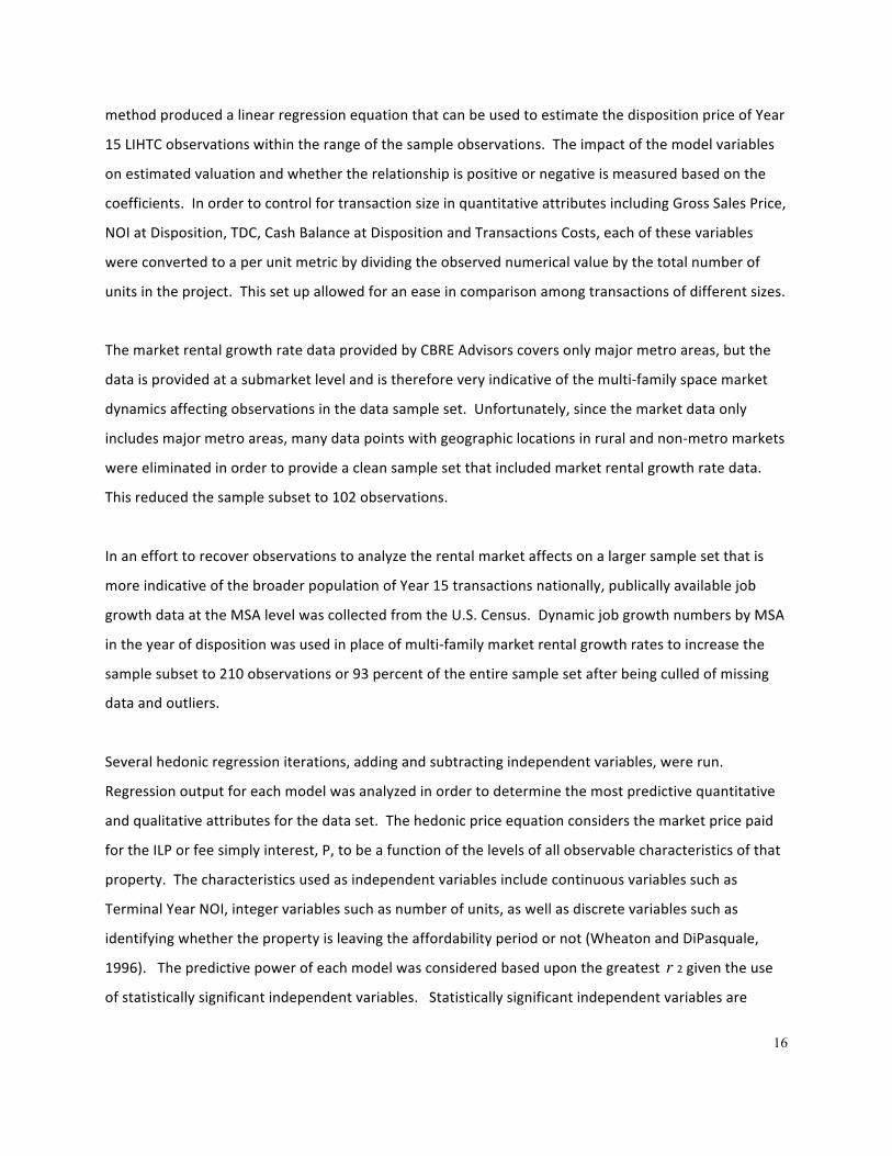
method produced a linear regression equation that can be used to estimate the disposition price of Year
15 LIHTC observations within the range of the sample observations. The impact of the model variables
on estimated valuation and whether the relationship is positive or negative is measured based on the
coefficients. In order to control for transaction size in quantitative attributes including Gross Sales Price,
NOI at Disposition, TDC, Cash Balance at Disposition and Transactions Costs, each of these variables
were converted to a per unit metric by dividing the observed numerical value by the total number of
units in the project. This set up allowed for an ease in comparison among transactions of different sizes.
The market rental growth rate data provided by CBRE Advisors covers only major metro areas, but the
data is provided at a submarket level and is therefore very indicative of the multi-‐family space market
dynamics affecting observations in the data sample set. Unfortunately, since the market data only
includes major metro areas, many data points with geographic locations in rural and non-‐metro markets
were eliminated in order to provide a clean sample set that included market rental growth rate data.
This reduced the sample subset to 102 observations.
In an effort to recover observations to analyze the rental market affects on a larger sample set that is
more indicative of the broader population of Year 15 transactions nationally, publically available job
growth data at the MSA level was collected from the U.S. Census. Dynamic job growth numbers by MSA
in the year of disposition was used in place of multi-‐family market rental growth rates to increase the
sample subset to 210 observations or 93 percent of the entire sample set after being culled of missing
data and outliers.
Several hedonic regression iterations, adding and subtracting independent variables, were run.
Regression output for each model was analyzed in order to determine the most predictive quantitative
and qualitative attributes for the data set. The hedonic price equation considers the market price paid
for the ILP or fee simply interest, P, to be a function of the levels of all observable characteristics of that
property. The characteristics used as independent variables include continuous variables such as
Terminal Year NOI, integer variables such as number of units, as well as discrete variables such as
identifying whether the property is leaving the affordability period or not (Wheaton and DiPasquale,
1996). The predictive power of each model was considered based upon the greatest r 2 given the use
of statistically significant independent variables. Statistically significant independent variables are

17
defined as those that have p-‐values below .05, which indicates the probability of obtaining a test
statistic at least as extreme as the observed test statistic. Independent variables included in the final
model are therefore deemed significant at a five percent confidence interval or in 95 percent of
observations.
Prior to running final regressions, the data was bifurcated into Rental Growth and Job Growth subsets as
described above. The inclusion of the LTV at Disposition independent variable was observed as a joint
causal and partially truncated predictive variable. Although the amount of the outstanding debt is
extremely predictive of value, since many dispositions have appraised values that are less than the
outstanding debt, the observed Gross Sales Price defaults to the amount of the outstanding debt.
As a result, the data subsets were further bifurcated into two additional subsets by eliminating
observations that had observed LTV at disposition of 0.97 or above. Hedonic Regression Analysis was
performed on the final four separate data subsets below and outputs was compared and analyzed.
1) Rent Growth with Truncated Dependent Variable Removed (“Model 1”)
2) Rent Growth with Truncated Observations Removed, but Including LTV at Dispo2 (“Model 2”)
3) Job Growth with Truncated Dependent Variable Removed (“Model 3”)
4) Job Growth with Truncated Observations Removed, but Including LTV at Dispo3 (“Model 4”)
1.4 Results & Interpretation
Across the four different regression methodologies the resulting y-‐intercepts and variable coefficients
reveal some interesting patterns. The y-‐intercept for Models 1 (3468.8284) and 3 (2634.4875) remain
relatively consistent, but drastically different from Models 2 (16959.2418 and 4 (14988.0169), which are
relatively consistent. This is intuitive because the subsets that include the LTV at Disposition variable in
the model experience a discounted y-‐intercept value related to the negative coefficient associated with
this variable.
2 “Truncated Observation” refers to those data points where an LTV at disposition was greater than or equal to 0.97. These were removed because it was observed that if a transaction is “under water,” the gross sales price reverts to the outstanding debt amount and is therefore all that is needed to predict gross sales price. This creates interaction affects in the model that distorts the predictive affects of other independent variables when analyzing observations of financially stable observations. 3 Ibid.

18
The coefficients for each independent variable remain fairly consistent across the four models as
opposed to the y-‐intercept. The TDC per unit variable is statistically significant across all models and the
associated coefficient ranges from .3873 in data subset 3 to .4972 in Model 2, suggesting consistent
depreciation of valuation through the Initial Compliance Period. The Terminal Year NOI per unit
variable is statistically significant across Models 1, 3 and 4 and ranges from 1.5471 to 3.7373. This is a
fairly significant range, but if you drop the coefficient from Model 2, which was statistically insignificant,
the range tightens to 3.3691 to 3.77373. Intuitively, Terminal Year NOI should be highly predictive of
valuation and thus the fact that this variable is not statistically significant in Model 2 calls into question
the validity of this model. The coefficient range for Models 1, 3 and 4 suggest a 3.37x to 3.77x valuation
multiplier on NOI, or a cap rate between 26.53 and 29.67 percent on sales of LIHTC ILP interests at Year
15. This suggests that Year 15 LIHTC transactions trade at a significant discount to their market rate
counterparts. The Cash Balance per unit variable is statistically significant across all four models and the
associated coefficient ranges from 3.3701 to 3.9142. This is a fairly tight range, but this coefficient is
deceivingly impactful as compared to the Terminal Year NOI coefficients because very few observations
in the sample have significant cash balances. The Affordability Expiration variable is statistically
significant across all four models and the coefficients range from 8238.5429 to 11434.6524, suggesting
that this dummy variable is consistently highly impactful on terminal valuation across all methodologies.
In comparing the Rent Growth models to the Job Growth models it is clear that the associated
respective coefficients for Rent Growth in Models 1 and 2 are in excess of the Job Growth coefficients in
Models 3 and 4. This suggests that Rental Growth Rates have a larger impact on valuation than Job
Growth Rates. The Job Growth models are further discounted by the fact that the Job Growth Rate
variable is statistically insignificant in both model iterations. As a result, the Job Growth Rate variable is
not considered useful in estimating terminal valuation. Thus, Models 3 and 4 are not useful in providing
affirmative insight on the subject topic.
The most statistically significant and predictive model is found using Model 1 above. The most
predictive variables for determining the sale price at disposition on or around Year 15 as dictated by this
model are the original TDC of the project, the terminal year NOI, the terminal year cash balance
including reserves, whether the project is subject to the extended use affordability period and the
submarket rental growth rate. These variables are able to account for 62 percent of the variation in the
19
overall sale price as determined by the r 2 in the model of .6236.
The Rental Growth Rate variable is only significant at a 96.4 percent confidence interval, while all other
variables are significant at a 99.99 percent confidence level. At a basic level, the estimated coefficients
on disposition observation characteristics (independent variables) may be interpreted as an implicit
price that buyers are willing to pay for more of each attribute (Wheaton and DiPasquale, 1996).
According to Model 1, the greatest determinant of valuation at Year 15 is the original TDC of the
property. This variable accounts for 48.56 percent of the total valuation. The second largest factor
based on the model is whether or not the project is leaving the Affordability Period. The model
indicates that LIHTC properties with expiring affordability requirements are worth $10,517.16 more per
unit. This component makes up 20.88 percent of the overall model estimated valuation, and represents
a valuation premium to properties subject to the Extended Use Period of 26.40 percent. The next
greatest factor in Year 15 valuation is the Terminal Year NOI. Since the income approach is the method
in which most income producing multi-‐family properties are valued, this certainly makes sense. This
variable contributes an additional $8,912.40 to the valuation making up 17.70 percent of the total value.
The submarket Rental Growth Rate variable contributes about the same as the Cash on Hand at Year 15
variable, with each contributing $1,563.03 and $1,440.58 respectively. Thus, the submarket Rental
Growth Rate contributes 3.10 percent to the valuation while the Cash on Hand variable contributes 2.86
percent to the valuation.4
4 The methodology used to arrive at values is explained in Section 5.2.
20
Chapter 2
Overview of the LIHTC program
2.1 LIHTC Production
The LIHTC program has been a significant source of multi-‐family housing production since its creation as
a part of the Tax Reform Act of 1986, which was enacted to replace substantial tax benefits for
affordable multi-‐family housing that were abolished under the same legislation (Abt Associates, 2012).
From 1987 through 2009, private developers and their investment partners leveraged the program to
create more than 2.2 million units of rental housing in more than 35,000 individual properties across the
United States and its territories. This accounts for about one-‐third of all multi-‐family housing
constructed during the same time period (Abt Associates, 2012). If you take into account the average
annual units Placed in Service in recent history (100,000 units annually), the program has generated
approximately 2.6 million units in its history. This is more than double the current public housing units
in service and makes the LIHTC the “largest program in U.S. history providing property-‐based subsidies
to rental housing, and since the early 1990s, has been the only such program developing substantial
numbers of additional units (Abt Associates, 2012: 2).” Its importance for the creation and preservation
of ethnically and socioeconomically diverse communities cannot be understated and for this reason the
program has enjoyed a long history of bipartisan support.

21
Figu
re 1: LIHTC
Tim
eline

22
2.1.1 The Making of an Industry
In the early years of the program developers paired the credit with Section 515 loans administered
through the Farmers Home Administration (FmHA) and ultimately its successor agency, the Rural
Housing Service (RHS), which is apart of Rural Development (“RD”) in the U.S. Department of Agriculture
(USDA). This program is a direct housing mortgage program provided to owner’s for the development of
housing for very-‐low-‐, low-‐ and moderate-‐income families, elderly persons and persons with disabilities.
These loans were particularly attractive because of their 30-‐year term, 50-‐year amortization rate and
below market interest rate, typically one percent. These transaction types made up 31 percent of the
projects over the first eight years of the program, which also saw rehabilitation projects make up more
than one-‐half of all projects (Abt Associates, 2012). This strategy largely fell out of favor after 1994. It is
important to note for this study that since Section 515 financed properties tended to be smaller in size
and were located in rural areas, these transactions were excluded from the subject sample set, as these
are not representative of the current or future properties that are reaching Year 15.
Another characteristic of the early formation of the program was the fund syndication practice of raising
equity investment capital from high net worth individuals as opposed to large institutional corporations.
This practice died as corporate investment demand for the credit greatly outstripped individual
investment demand driving up credit prices and driving down investment yields to a level that became
unattractive for most individual investors. The growth in corporate demand for credits was largely the
result of the passing of the Gramm-‐Leach-‐Bliley Act in 1999, which repealed part of the Glass-‐Steagal Act
of 1933, removing barriers to corporate consolidation in the banking and financial industries and a
subsequent widespread focus on meeting the requirements of the Community Reinvestment Act of
1977 (CRA). The CRA originally was passed to prevent lending institutions from discriminating against
low-‐income persons by requiring them to extend a certain percentage of their loans to low-‐income
persons in the communities in which they did business. Corporate interest in LIHTC investment
exploded after 1999 when CRA examination scores became a common hindrance to regulatory approval
of financial institution mergers and acquisitions. As an investment with one of the highest risk-‐adjusted
returns qualifying under the CRA, it is clear why demand for the credit exploded after 1999. As the
program entered the 21st century, institutional demand for the credit outstripped supply for the first
time creating an increasingly efficient and effective tool for the creation of Affordable Housing. Figure 2
below depicts the evolution of tax credit pricing and investor returns through the maturity of the

23
industry.
Figure 2: Tax Credit Pricing and Investor IRR Time Series
2.1.2 The Modern Era
Although LIHTC industry underwriting standards and financial structures common in the business were
in wide use throughout the mid-‐ to late 1990s, there was still a gap in understanding of what the overall
LIHTC portfolio looked like and thus the effectiveness of such standards and structures. In 1996, HUD
led the push for data aggregation in the industry when they commissioned Abt Associates to take an
inventory of all LIHTC properties built between 1992 and 1994 and many from before 1992. In 1999,
building on this catalogue, Cummings and DiPasquale conducted a study that was published in Housing
Policy Debate titled “The Low-‐Income Housing Tax Credit, An Analysis of the First Ten Years,” which
provided a detailed statistical analysis of what had become a multi-‐billion dollar industry. In 1999, the
preservation discussion had just begun. With the first transactions reaching the end of the Initial
Compliance Period in 2002, project outcomes post compliance were very uncertain. In addition, since
transactions placed in service in 1990 and before were not subject to an additional Extended Use Period,
preservation became a particular concern for properties reaching Year 15 between 2002 and 2005.
Source: Ernst & Young (2003)

24
2.1.3 The Preservation Era
A 2007 Massachusetts Institute of Technology Master of Science in Real Estate Development thesis by
Lillian Lew-‐Hailer explored the outcomes of this era of Year 15 transactions in Massachusetts by relating
the market and programmatic dynamics to other HUD housing legacy programs, which had reached
similar preservation transitions in the face of expiring affordability requirements. She compared the
preservation conundrum of this era with the expiration of affordability requirements in the HUD
221(d)(3) and 236 programs. The 221(d)(3) program offered direct loans to developers at below market
interest rates while the 236 program was an indirect loan structure administered through private
lenders facilitated by offering HUD mortgage insurance and interest reduction payments (IRO) to lenders
in exchange for charging a below market interest rate. In the case of both programs, owners committed
to setting aside units for low-‐income tenants at rents below market rates. These loan programs had a
similar sunrise to the first iteration of the LIHTC program as the loans could be pre-‐paid without penalty
after 20 years. In the early 1980s, when the first group of 221(d)(3) and 236 loans reached the end of
the prepayment lockout, several developers opted to prepay their loans and exit the program to reap
the benefits of higher market rents. Housing advocacy groups succeeded in suspending this option with
the passing of the Low-‐Income Housing Preservation Act of 1987 (ELIHPA) and the Low-‐Income Housing
Preservation and Resident Act of 1990 (LIHPRHA), but they were ultimately unable to win the legislative
battle with angry developers who felt that the terms of the program had been changed materially to
their detriment. As of 2002, the National Housing Trust estimated that 60,000 units have been lost
since the elimination of federal preservation programs aimed at protecting affordable housing assets
created by these two programs (Achtenberg, 2002: 3).
It is estimated that five percent of projects that reached Year 15 of the LIHTC program between 2002
and 2006, most of which would not have been subject to the Extended Use Period, were converted to
market rate housing equating to at least 50,000 affordable units lost (Ernst and Young, 2010: 27).
Considering there was no legal framework in place to ensure the preservation of these units, the
amount of units lost would not be a cause for alarm if the United States were not in the midst of an
affordable housing crisis. In a 2012 study conducted by the National Low Income Housing Coalition
(NLIHC) titled “Out of Reach 2012: America’s Forgotten Housing Crisis,” it is estimated that as of 2010,
9.8 million American renter households (one in four) were unable to find affordable housing as defined
by HUD (annual rent less than 30 percent of gross median income) based upon the prevailing Fair

25
Market Rent and AMI in respective markets. This equates to an additional 6.8 million units needed
nationwide, which is an incredibly large shortfall given our most successful and prolific program for the
creation of new Affordable Housing, the LIHTC program, is only producing roughly 100,000 new units
per year. Based on need and the extensive pipeline of aging LIHTC transactions, it is clear that the LIHTC
industry has entered an era where preservation is paramount.
2.2 Basic Transaction Structure and Process
The LIHTC program’s success can largely be attributed to its elegance in blending the most useful tools
for housing production from the public and private sectors into one efficient program. The federal
government, through the Tax Reform Act of 1986, created a tax credit for the creation of low-‐income
housing that can be used by developers or investors of qualified affordable housing to offset ordinary or
business income. At a most basic level, a tax credit is awarded for each dollar invested to create
qualified Affordable Housing. In practice, the process is far more complex and warrants further written
explanation and graphical illustration, which follows.
26
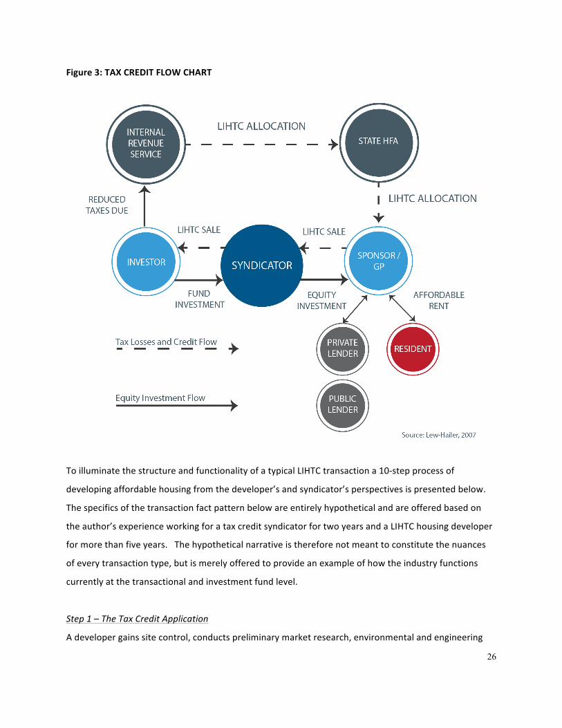
Figure 3: TAX CREDIT FLOW CHART
To illuminate the structure and functionality of a typical LIHTC transaction a 10-‐step process of
developing affordable housing from the developer’s and syndicator’s perspectives is presented below.
The specifics of the transaction fact pattern below are entirely hypothetical and are offered based on
the author’s experience working for a tax credit syndicator for two years and a LIHTC housing developer
for more than five years. The hypothetical narrative is therefore not meant to constitute the nuances
of every transaction type, but is merely offered to provide an example of how the industry functions
currently at the transactional and investment fund level.
Step 1 – The Tax Credit Application
A developer gains site control, conducts preliminary market research, environmental and engineering

27
investigation and financial modeling and underwriting, among other predevelopment functions. If the
deal is deemed to be viable, this predevelopment work product will be collated into a competitive tax
credit application submission. In this example, it is assumed that the developer is pursuing a nine
percent credit allocation, which is indicative of the Applicable Federal Rate that will be applied to the
Eligible Basis to arrive at the annual allocation of tax credits awarded to the project. This will account
for roughly 70 percent of the project cost on a present value basis, but will be monetized at a rate closer
to 60 percent of the project cost. This distinction is made because there are also non-‐competitive four
percent tax credits that are allocated through a different process and are often very different in their
financial structure.
Step 2 – HFA Application Review and Scoring
The Housing Finance Agency (HFA) in the respective state in which the project is located will receive this
application and review it in conjunction with all other applications submitted within an allocation year.
The HFA is a function of the state government that is given annual allocating authority by the Internal
Revenue Service on a per capita basis. In 2013, states were given allocating authority equal to the
greater of $2.25 per capita or $2,590,000 (Housing Advisory Group, 2013). The HFA will review
applications and score them objectively based upon scoring criteria contained within their Qualified
Allocation Plan (QAP), which states have the authority to develop as they see fit to help ensure
submitted projects meet the unique programmatic goals of each respective state. The QAP must of
course work within the regulatory framework of the LIHTC program, which is governed by Section 42 of
the Internal Revenue Code, but QAPs can differ drastically from state to state, which is reflective of the
unique affordable housing challenges faced by different parts of the country. At this point, the HFA is
also paying particular attention to the financial viability and regulatory compliance of each proposed
deal including compliance with per unit cost limits and a thorough subsidy layering review to ensure that
they do not award more subsidy to a project than it needs. Any application that does not meet these
threshold requirements will not be considered for the scoring portion of the review.
Step 3 – Tax Credit Awards
Once the HFA has objectively scored applications, allocations will be awarded to for-‐profit and not-‐for-‐
profit developers in the lesser of a predetermined per project or per sponsor maximum allocation
amount as dictated by the QAP or the amount of credit their project qualifies for based upon the

28
number of affordable units constructed as determined by the corresponding Eligible Basis. Since
projects are scored, there is a ranking based on the application score and the HFA will award credits
starting at the top of the ranking until their allocating authority in a given year is exhausted.
Step 4 – Predevelopment and Financing Procurement
With an allocation in hand, the developer now has a real deal. Since developers typically underwrite
applications assuming they are successful in receiving credits, few projects that fail to receive credits will
be financially viable and therefore most will die. Those that receive credits will move forward
immediately with complete architectural drawings and the permitting process with the intent to begin
construction of the project within six months. They will also market their credits to Syndicators and
Direct Investors as well as construction and permanent lenders. They may also have subordinate
financing commitments from state or local authorities that need to be secured or finalized. It is not
uncommon for a LIHTC transaction to have four or more layers of financing, which creates significant
complexity in the deal structuring and closing process. With regard to the credits, the LIHTC program is
structured so that credits flow to owners over a ten-‐year period and allocations are usually several
million dollars so there are few developers that have enough federal tax liability to make use of the
credits. As a result, they seek to sell the credits to raise equity investment capital.
Stage 5 – Due Diligence Process and Closing
Once a Direct Investor or Syndicator is selected by the developer, the investor will typically require a
long list of due diligence items in an effort to mitigate risk and ensure the quality of the investment
opportunity. Most Syndicators and Direct Investors, either through staffing or third parties, conduct
their own construction and architectural plan review, market study, appraisal, financial analysis,
accounting and legal work. This private sector discipline has been sighted by many as one of the keys to
the success of the program.
Syndicators or Direct Investors must be active investors in the partnership that undertakes the project
and must remain in the transaction for the 15-‐year Initial Compliance Period to avoid tax credit
recapture liability with the IRS. This long hold period also reduces the pool of interested investors. If
the developer partners with a syndication company, they will likely sell the credits into a nationally
diversified tax credit fund or a proprietary tax credit fund. This process involves two separate

29
partnerships, which often are referred to as the “Lower Tier” and “Upper Tier” partnership. The Lower
Tier refers to the partnership between the Developer/GP and the Syndicator (typically 0.01 percent
owned by the GP and 99.99 percent owned by the syndicator) and the Upper Tier refers to the
partnership between the Syndicator and the investor or end user of the tax credits (typically 0.01
percent owned by the Syndicator and 99.98 percent owned by the investor). It is through this process
that the tax credit benefits can be passed through to the banks or insurance companies with the
predictable tax exposure to benefit from them, while the developer receives the equity capital needed
to undertake his projects. This closing process can occur as a simultaneous closing of both the Lower
and Upper Tier partnerships, but more often the Lower Tier partnership is closed, which is then made a
part of a fund that closes at a later date once the fund is fully specified with other Lower Tier
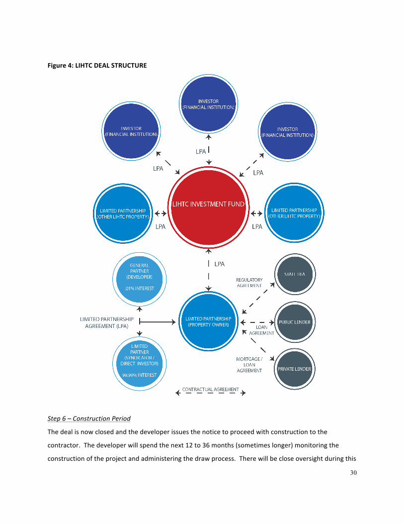
partnerships that own other Affordable Housing properties. Figure 4 below graphically illustrates the
typical deal structure.
30
Figure 4: LIHTC DEAL STRUCTURE
Step 6 – Construction Period
The deal is now closed and the developer issues the notice to proceed with construction to the
contractor. The developer will spend the next 12 to 36 months (sometimes longer) monitoring the
construction of the project and administering the draw process. There will be close oversight during this

31
period from the construction lender and Syndicator to ensure the quality of the construction
workmanship and consistency with plans and specifications.
Step 7 – Lease-‐up Period
Once the project has been fully constructed and the municipality issues certificates of occupancy, the
project is considered to be “Placed in Service” and can now be occupied by qualified tenants. Many
developers have their own property management companies that have a compliance function, but this
service can also be outsourced to a third party. Whatever the case, the compliance team will review W-‐
2s, tax returns, child support, disability payments and any other form of income that each resident has
to ensure their eligibility to live in the new community, based upon the affordability levels stipulated
and agreed to by the developer in the original tax credit application submission.
Step 8 – Stabilization and Permanent Loan Closing
Once the community is fully occupied, it is said to have reached “Qualified Occupancy” and tax credits
can begin to flow through to the investor. At this point the construction and lease-‐up risk is behind all
parties to the transaction, and the developer can move to close its permanent financing and pay off the
construction loan. The transaction has entered the asset management stage and begun the 15-‐year
Initial Compliance Period.
Step 9 – Asset Management and Compliance Monitoring
During this period, the developer operates the property and faces significant guarantee exposure to the
ILP for any issues that arise during the compliance period that cause the property’s operations to fall
below break-‐even. This is commonly referred to as an Operating Deficit Guarantee and is typically in
place for a significant portion of the 10-‐year Credit Period. It requires the developer and its affiliates to
fund any operating deficits that arise for whatever reason. The vast majority of transactions have a
funded Operating Deficit Reserve among other reserves (replacement reserves, subsidy reserves, etc.)
that are controlled by the Syndicator and to backstop additionally the developer’s personal guarantee.
In addition to an Operating Deficit Guarantee, the developer also provides a tax credit guarantee and
completion guarantee. The former puts the burden of tax credit recapture by the IRS as the result of
falling out of compliance with the LIHTC program on the developer. The latter, which has typically
“burned-‐off” at this juncture, puts the liability to complete construction of the project in the case of cost

32
overruns on the developer as well. Needless to say, the developer has significant incentive to maintain
the successful operation of the property as a compliant Affordable Housing project as committed to in
the original tax credit application. The asset management function of the Syndicator will monitor the
operation and physical condition of the property as well and take action to protect their investment if
they feel that the developer is not capable of performing this function. In fact, all LIHTC partnership
agreements will contain developer removal and replacement rights for the Syndicator. In addition, the
HFA for the state in which the project is located will perform an annual compliance audit of the
property, which includes an inspection of the physical condition and a review of tenant files to ensure
compliance with rental and income restrictions. The developer’s motivation during this period is one of
risk mitigation versus cash flow or rent growth, as the downside risk is far greater than any upside one
can gain via operating the property more efficiently.
Step 10 -‐ Year 15 and the Limited Partner Exit
After the first 10 years of operation, tax credits cease to flow and the vast majority of the Direct Investor
or Syndicator’s projected financial benefits have been received. Many investors will exercise a put
option after the credit period, which allows them to exit the transaction during the Initial Compliance
Period while retaining indemnity from recapture from the developer, who basically commits to remain
in compliance despite lack of investor asset management oversight. After credits cease to flow, the
investor only reaps tax benefits typical of conventional real estate through the value of the real estate
depreciation deduction, but, more often, the property becomes a non-‐performing asset on the
investor’s balance sheet. Since the investor pursues LIHTC investments for the tax benefits, surplus cash
flow is often seen as a negative because this dilutes tax loss benefits. This is countered by the need to
maintain a financially healthy property through the duration of the 15-‐year compliance period to avoid
tax credit recapture from the IRS. This results in financial structures that lead to razor thin profit
margins that can be highly susceptible to market fluctuations. This is discussed further in Chapter 3, but
this, in particular, impacts the options for developers and investors at Year 15. Syndicators typically
build tax credit investment funds with properties in a tight vintage range so that they are able to dispose
of limited partnership interests and wind down the fund within a two-‐year period. For those investors
that choose to remain in the transaction through the compliance period, profitable exit options are
often limited. The end buyer will be anxious to get the transaction off of his balance sheet after Year 15,
and he was never expecting any significant portion of his return to come from the disposition, so, often

33
times, the speed of disposition becomes a priority versus maximizing value. The typical Year 15 exit
strategies prevalent in the industry are discussed in Section 2.3.
The effectiveness of the program is routed in its public-‐private partnership structure. Cummings and
DiPasquale put it best when they described the elegance of the program structure in their seminal
paper, “The Low Income Housing Tax Credit: An Analysis of the First Ten Years”. "By bringing these
various actors together, the LIHTC program is designed to bring the efficiency and discipline of the
private market to the building of affordable rental housing. Investor participation is expected to add
further oversight to the program, since return to the investors is dependent on the project’s staying in
compliance. By allocating the tax credits through the states, the program provides the flexibility to build
housing that meets local market needs (Cummings and DiPasquale, 1999: 252)." The program’s success
is largely unquestioned in literature, but the flood of transactions that are now reaching the end of the
compliance period and the impending expiration of affordability land use restrictions beginning in 2018
have put a microscope on preservation. Although Abt Associates’ recent analysis suggests that most
properties exiting the program are maintained as Affordable Housing, there is reason to believe that this
could change as rental markets across the country continue to gain strength and developers face limited
viable preservation options.
2.3 Year 15 Exit Options
Year 15 is a common time to have a recapitalization event because ownership is likely to change as the
ILP seeks to dispose of an asset they have received all expected benefits from and original owners can
sell their interest without being liable for a subsequent failure to maintain affordability by the buyer
(Schwartz and Meléndez, 2008). This trend is almost certain to continue into the future and beginning in
2020, several thousand units will be hitting year 30 and exiting the Extended Use Period while 100,000
units per year will reach Year 15 annually, creating a massive pipeline of recapitalizations with limited
viable options. As the national LIHTC portfolio matures, one dispositions director for a national tax
credit syndicator predicted that the public policy pressure to layer-‐in deep affordability units that began
10 years ago, will result in the vast majority of year 15 transactions being valued at an amount that is
less than the outstanding debt and accrued interest. They indicated that additional soft subordinate
debt that was layered-‐in to deal capital stacks in order to allow for smaller amounts of must-‐pay hard
debt (given less cash flow to cover the associated debt service as a result of deep affordability
34
requirements) leads to negatively amortizing debt structures (Anonymous Interview, 2013). This may
require us to re-‐think the current disposition strategies used industry-‐wide. Those currently in practice,
many of which are actually written into limited partnership agreements to assist in adding certainty for
the partners about the nature of the exit, are outlined below.
Bargain Sale and Charitable Contribution
This strategy is commonly written into limited partnership agreements on transactions with non-‐profit
partners whereby the exiting ILP agrees to accept a sale price that is equal to the amount of the
outstanding debt obligations. This can only be executed if the appraised value of the property exceeds
the amount of the outstanding debt. To complete the exit, the non-‐profit either agrees to have the debt
assigned to them or secures refinancing dollars to pay off the existing debt. The difference between the
appraised value and the outstanding debt is then considered to be a charitable contribution by the for-‐
profit exiting ILP to the acquiring non-‐profit GP (Lew-‐Hailer, 2007). This strategy can be beneficial for
both parties if the GP is interested in continuing to own and maintain the property as Affordable
Housing and the ILP can make use of the tax benefits associated with the charitable contribution while
purging their balance sheet of an underperforming asset. This could, however, lead to a taxable event
for the LIHTC partnership if the sales price exceeds the book value of the asset, which would result in a
gain on sale on the portion of the property sold (Novogradac, 2011). This would typically become the
responsibility of the non-‐profit GP as dictated by the LPA, which could prove problematic depending on
the size of the tax bill. In addition, if the appraised value of the property is less than the outstanding
debt on the property, then this strategy is rendered useless and the acquisition of the ILP interest
through a transfer or other charitable methods becomes far less attractive for the GP or even a third-‐
party since an assumption of debt in excess of value is in most cases a liability as opposed to an asset.
The exception is if a third party believed they could reposition the asset or improve operations to add
value, but the ability to execute such a strategy is greatly diminished by the Extended Use Period, which
will extend affordability requirements and thus depress rents for an additional 15 years.
Debt Plus Taxes
This strategy is also implemented primarily when non-‐profit entities are a part of the ownership
structure. This was included in many post-‐1990 LPAs when the IRS changed the regulations that govern
the length of the compliance period (Lew-‐Hailer, 2007). They simultaneously added the Extended Use

35
requirement while allowing for some tax relief for ILPs who agree to dispose of their interest at a below
market price. This was meant to act as a preservation tool to encourage an ILP to exit via a sale to a
non-‐profit who is likely to continue to maintain the property as Affordable Housing. The exit price
becomes the amount of the outstanding debt plus any Exit Taxes associated with the disposition. Exit
Taxes are incurred by the ILP when their Capital Account is negative at the time of disposition or if the
sale price exceeds the outstanding debt encumbering the asset (LISC, 2006). This outcome is likely if the
property is operating reasonably well and is subject to the Extended Use Period. This strategy also
becomes complicated and unattractive from the GP’s perspective if the property is worth less than
outstanding debt because an underperforming asset is considered more of a liability and the GP is
therefore unwilling to pay the investor’s Exit Taxes. In this scenario, the Limited Partner Interest
Transfer described below is more likely.
Limited Partnership Interest Transfer or Sale
This strategy and, in particular, a transfer of the ILP interest is most often employed by an investor when
the property is an underperforming asset. If the property is operating at or near break-‐even and is
overleveraged, the property’s outstanding debt will exceed its market value. In this case, the investor
will want to purge the books in the least expensive manner possible and if the Syndicator is a non-‐profit,
a transfer of the ILP to the GP is the most efficient way. Also, a transfer can often be less complicated
because the partnership can avoid triggering debt repayment clauses in respective loan agreements that
would come in a sale. The reserve account balances also remain in the ownership of the partnership as
opposed to being disbursed in full in conjunction with a sale (Lew-‐Hailer, 2007). This might seem like a
decent outcome for the GP if the property is in good physical condition and occupancy is stable enough
to continue to maintain the property with little or no capital improvements. Even in this case, a
recapitalization would be triggered by the expiration of the first priority loan term, which could follow in
one to three years if the debt source is private in nature. This exit also puts the future viability of the
property in question in the out years of the Extended Use Period.
Third Party Fee Simple Property Sale
If the GP is in agreement to sell their interest, the ILP exit can occur in conjunction with a sale of the
property. In this case the partnership would convey the property to the new owner and the partnership
would be dissolved. The Land Use Restriction Agreement (LURA), which binds the new owner to the

36
Extended Use Period, trails with the land and therefore remains in effect. This exit will only occur with
financially viable properties that are in stable real estate markets. This could also occur if a property is
underperforming relative to its potential as a result of mismanagement and a third-‐party believes they
can add value through improved management or repositioning, while still remaining subject to the
affordability provisions. It is likely that the fee simple sales of LIHTC properties will accelerate in the
years leading up to the expiration of the Extended Use Period, often subsequent to an alternative Year
15 exit. The first wave of year 30 transactions will come at the latter part of this decade and will
continue annually at an increasing rate. Abt Associates’ 2012 interview-‐based study reported that,
"brokers and industry observers speculate that later year LIHTC properties will prove more difficult than
early year properties to refinance and move into the conventional real estate world—either with
affordable rents or with repositioned, higher rents. The upshot may be that a larger percentage of later
year LIHTC properties end up being recapitalized with additional allocations of nine percent tax credits
(Abt Associates, 2012: 77)." The opportunity to recapitalize Year 15 projects with nine percent tax
credits is exceedingly competitive with a very limited amount of resources. Furthermore, rehab
properties remain less attractive to investors and will therefore receive less equity per dollar of credit as
the investor requires a higher investment return to compensate for the risk associated with the out
years of a rehabbed property. A viable option in many markets is the use of non-‐competitive 4 percent
credits, which allow for the acquisition book value to be included in the tax credit basis along with any
rehab scope of work. This option can still be difficult to execute on given the smaller amount of equity
that is raised with 4 percent credits and the aforementioned lack of investor interest in lightly improved
rehabilitation properties. Clearly more options are needed at Year 15 for the modern wave of LIHTC
properties exiting the Initial Compliance and Extended Use Periods. Figure 5 below shows the current
likely outcomes based on different fact patterns.
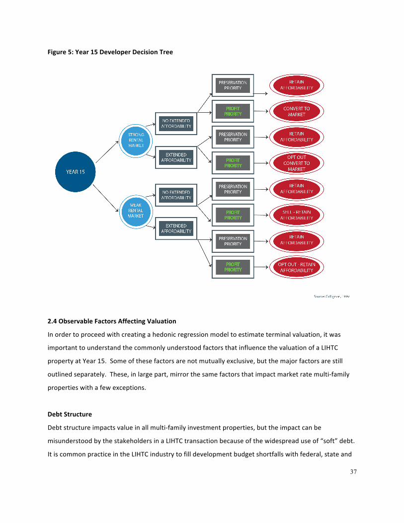
37
Figure 5: Year 15 Developer Decision Tree
2.4 Observable Factors Affecting Valuation
In order to proceed with creating a hedonic regression model to estimate terminal valuation, it was
important to understand the commonly understood factors that influence the valuation of a LIHTC
property at Year 15. Some of these factors are not mutually exclusive, but the major factors are still
outlined separately. These, in large part, mirror the same factors that impact market rate multi-‐family
properties with a few exceptions.
Debt Structure
Debt structure impacts value in all multi-‐family investment properties, but the impact can be
misunderstood by the stakeholders in a LIHTC transaction because of the widespread use of “soft” debt.
It is common practice in the LIHTC industry to fill development budget shortfalls with federal, state and

38
local sources of soft debt that are available to support the construction or preservation of Affordable
Housing. Some sources include federally appropriated HOME and Community Development Block Grant
(CDBG) funds via HUD. These are appropriated to HUD by the federal government annually and then
allocated to states and city government agencies to be committed to projects that meet programmatic
requirements. These soft debt sources are real debt that must be repaid by the end of the loan term,
but commonly come with below market interest rates, can be subordinated to other notes as it relates
to the priority for repayment and also often are serviced subject to availability of cash flow. The layering
of debt in a complicated mixed-‐finance transaction becomes necessary in high cost markets or when the
market demand for tax credits is soft, which drops the credit pricing and thus equity portion of the
capital structure. It is also necessary when QAPs issued by HFAs contain criteria requiring developers to
commit to deep affordability requirements to have a competitive application. To set aside units for
those that earn up to 30 percent of AMI as opposed to the programmatic requirement of 60 percent of
AMI essentially cuts in half the maximum rent in which a developer can charge, while holding operating
expenses constant. This, of course, contributes to an inability to support large amounts of conventional
debt at market level interest rates.
Although common prior to the financial crisis, the use of several layers of debt became requisite in the
majority of transactions after 2008. Tax credit pricing dropped from the mid $0.90s to the mid $0.70s,
with investor demand all but non-‐existent as losses from other financial activity more than offset many
corporations’ federal tax exposure. The result in the vast majority of these transactions is insufficient
cash flow to support soft subordinate notes. Even if interest rates are below market, if unpaid, the
interest typically accrues and becomes part of the outstanding balance of the loan resulting in the
negative amortization of the note. Given payments are only required if cash flow is sufficient to pay
them, negative amortization is not impactful during the Initial Compliance Period of a LIHTC property.
This practice does, however, contribute significantly to a large percentage of transactions having a
terminal value that is less than the amount of outstanding debt. Based on the 223 observations in the
data sample, 29 percent experienced negative amortization or were unable to service debt sufficiently
to reduce the outstanding debt balance during the Initial Compliance Period. This makes refinancing all
but impossible at Year 15 and greatly diminishes the value of the property and options for preservation.
It was not possible to measure the impact on valuation of this variable in this study due to its mutual
causality with observed price, which is discussed further in Chapter 4.
39
Affordability Requirements
The affordability requirements in a LIHTC transaction can by bifurcated into two categories: that which
affects the term of affordability and that which affects the level of affordability. That being said, it is
important to note that whatever level of affordability one commits to ultimately, it will be in place for
the programmatic term. The term of affordability is largely standardized through Section 42 of the
Internal Revenue Code, requiring that transactions accepting LIHTC’s remain affordable for a period of
30 years (the Initial Compliance and Extended Use Periods). This requirement is programmatic in nature
and greatly impacts value intuitively and as evidenced by the regression results. It should be noted,
however, that in markets where the maximum LIHTC rents approximate the prevailing market rent for
unrestricted multi-‐family properties, the affordability requirement will have much less impact since the
market is the primary driver of achievable rent levels versus the programmatic rent cap (Abt Associates,
2012). This condition exists primarily in rural and other low cost markets with low barriers to entry.
The level of affordability is also programmatic in nature with developers having the choice of setting
aside 20 percent of units for those that earn up to 50 percent of AMI or 40 percent of units for those
that earn up to 60 percent of AMI. In practice, almost all LIHTC financed transactions exceed these
baseline requirements by a large margin in order to maximize their tax credit allocation and to minimize
the market risk of the transaction. Investors and Syndicators become nervous about a mixed-‐income
project that includes greater than 35 percent of the units as market rate, given the concern related to
attracting renters with more choice (given greater income) to a LIHTC community and the significantly
large portion of the NOI that will depend on the ability to attract these renters. Where affordability
requirements start to significantly affect value is when deep affordability income bands are included in
the unit set-‐aside mix. It is important to note that these elections are made voluntarily by the developer
to either ensure a competitive LIHTC application or in order to qualify for some additional soft
subordinate debt award. Often the drag on NOI caused by deeper affordability set-‐asides is more than
offset by the size of the subordinate debt award. In other cases, the competition for nine percent
credits in some states is so fierce that developers will commit to set aside deeper affordability units
without receiving any additional subsidy, which can endanger the long-‐term operational viability of the
project. In either case, the commitment to lower the income earning potential of the property even
more than the programmatic requirements is a recipe for devaluation that often leads to an upside

40
down capital structure at Year 15. The impact of the affordability term is tested in the model via the
affordability expiration dummy variable. Since the affordability level ultimately impacts the NOI per
unit, its impact is measured via the NOI at disposition variable.
Subject Market Conditions
The rental market conditions impact LIHTC properties in the same manner that they impact market rate
properties. Mixed-‐income LIHTC transactions with a higher percentage of market rate units are thought
to be particularly vulnerable to increased vacancy caused by an oversupply of units or exogenous
economic factors. On the contrary, 100 percent affordable LIHTC properties are thought to be
somewhat insulated from rental market risk dynamics because the rents charged typically are below the
prevailing market rents as it is. This is less common in weaker rental markets where market and
affordable rents are similar. For Year 15 transactions subject to the Extended Use Period with majority
or 100 percent affordable units, a positive rent growth outlook in the subject submarket should have
little affect on the valuation of the property at exit if max LIHTC rents are already being achieved
because of statutory limitations to rent increases. In markets where the market rent advantage enjoyed
by LIHTC properties is non-‐existent, Abt and Associates noted that “Owners of properties…whether they
are original sponsors or new purchasers, often describe these properties’ post-‐Year 15 LIHTC status as
irrelevant (Abt Associates, 2012: 50)." The local rental market condition will likely become more
important and impactful on valuation as the first wave of transactions reaches year 30 in 2020. The
rental market impact on valuation is measured in the model using submarket rental growth rates in
the year of disposition as an independent variable.
Poor Property Management
As with any asset, poor management can significantly impact value. There is nothing observable that
predisposes LIHTC transactions to have poor managers, but the compliance requirements can make
LIHTC asset management more challenging than conventional market rate multi-‐family management. In
fact, it is proven empirically that LIHTC multi-‐family properties tend to run higher expense levels than
their conventional counterparts, which may be the result of the added expenses associated with
compliance and tenant screening (Ernst and Young, 2010). In general, understanding whether
underperformance is the result of poor management can be hard to isolate and measure empirically.
It is assumed that the Terminal Year NOI variable has the affects of poor management included in it.
41
Tenancy Type
It can be observed empirically that elderly communities tend to have lower delinquency rates, higher
stabilized occupancy, higher debt coverage ratios and cash flow per unit relative to other tenancy types
(Ernst and Young, 2010). This should technically lead to a more valuable property versus a family,
special needs or mixed tenancy property. This impact is measured through the use of dummy variables
for each tenancy type: elderly, family and mixed. It is reasonable to assume that these operating
factors would also be reflected in the Terminal Year NOI variable.
Construction Type
This attribute refers to whether the project is a rehab or a new construction project. In theory, if the
rehabilitation construction scope is significant enough, there should be zero incremental observable
impact on terminal value. In several recent studies of the national LIHTC portfolio, rehab properties are
observed to underperform in the latter part of the Initial Compliance Period (Ernst and Young, 2010).
This would stand to reason if a light rehab was conducted and capital needs pile up. This could also
manifest itself through the changing tastes of housing consumers who have come to expect larger sized
units, which older rehabbed properties may not have, due to the fact that unit dimensions were
originally set in stone in the 1970s or earlier. The impact of the construction type on value is measured
by using dummy variables for each construction type in the sample: historic rehab, rehab, new. It is
also reasonable to assume in this case, that the affects of physically uncompetitive properties would
be reflected in the Terminal Year NOI variable as occupancy falls given a lack of market demand for an
inferior product.
Regional Location
Of course, location is typically one of the most important aspects of real estate value. To consider this
attribute, the data sample was regionalized by observation to create five dummy variables: Northeast,
Southeast, Southwest, Midwest and West. Since real estate markets are very local and one
submarket within a particular city can vary drastically from another, this metric attempts to
understand whether the cost of living, operating expenses and construction cost differences among
regions in the U.S. have an impact on the terminal value of a LIHTC transaction.

42
Project Size
This attribute’s impact on valuation is derived from the economies of scale achieved through spreading
fixed operating costs across a larger number of units in a single project. This also attempts to capture
whether there is a valuation premium that may be derived from institutional investment interest and
thus liquidity in the disposition market for larger communities. Abt and Associates note in their 2012
study "that most of the properties that end up sold to third parties appear to be among the largest in
the LIHTC portfolio [and that] one broker reports 100 units as the average size of Year 15 deals that they
sell (Abt Associates, 2012: 34).” Year 15 fee simple property interest sales to third parties will almost
always drive valuation higher than other exit alternatives discussed, so it is logical to consider
whether this variable impacts valuation empirically. To explore this, the quantitative number of units
in the project was used as an independent variable.

43
Chapter 3
Literature Review – The Low Income Housing Tax Credit Program
There has been relatively little analytical research performed on the LIHTC program when you consider
it is approaching its 30th year of existence. In addition, much of the literature to date has focused on
interview and survey-‐based methods of research to draw conclusions about how the industry functions.
The empirically backed literature has largely focused on the efficiency and effectiveness of the program
given the significant commitment of public tax dollars ($7.04 Billion annually5) committed to the
program through forgone tax revenues. In the context of the industry, efficiency has typically been
measured by studying what percentage of each forgone tax dollar actually gets invested into the
construction of Affordable Housing. Efficiency has increased significantly as the industry has matured
with tax credit pricing increasing from 50 cents per dollar of tax credits in 1987 to more than 90 cents
per dollar for properties placed in service in 2006 (Ernest & Young, 2010). The research in this study
focuses specifically on the effectiveness of the program as it relates to the disposition of LIHTC assets as
they reach the end of the Initial Compliance Period. Abt Associates 2012 HUD commissioned study is
the most relevant and current research on this specific topic. The core research question in that study is
whether pre-‐1990 LIHTC transactions are preserved as Affordable Housing despite the affordability
requirement sunrise. This study also looked at the spectrum of outcomes for LIHTC transactions
reaching the end of the Initial Compliance Period. The apparent intent of the Abt Associates study is to
understand where program or industry underwriting deficiencies may lie, which will undermine the
ability for LIHTC units to remain affordable. To date, there has been little research focused on the
consistent lack of residual value in LIHTC transactions and the corresponding impact on their long-‐term
viability, which is the main focus of this research.
3.1 Effectiveness of Program Structure
As discussed previously, the LIHTC program as a whole is widely considered by academics, politicians
and housing experts to be the most successful mechanism for the creation of new Affordable Housing
units in the history of the United States. Certainly relative to other HUD legacy programs, the success
and efficiency is unmatched, but the program is not without its issues, which several recent studies have

44
highlighted. The literature review below focuses on research related to the program structure’s impact
on Year 15 valuation and exit options.
Erosion of Market Advantage Over Time
When LIHTC units are first placed in service, they are usually indistinguishable from market rate multi-‐
family properties in the same submarket. As a result, in the early years of operation, LIHTC rents are far
less than implied market rents given their high quality relative to the price point. Burge conducted a
recent study of this phenomenon and determined that this market advantage eroded as the properties
aged and declined in quality during the Initial Compliance Period (Burge, 2011). Given the extended
hold period for a LIHTC investment as governed by the IRS compliance rules, it is exceedingly difficult for
LIHTC owners to keep their properties competitive in the marketplace. Abt Associates noted that since
“LIHTC properties are expected to operate for 15 years without raising capital for repairs by refinancing
[and] LIHTC reserves—constrained by the property’s projected cash flow—generally are not funded at a
high enough level to cover capital needs that arise over that period,” the physical condition of LIHTC
properties can be quite poor at Year 15 (Abt Associates, 2012: 12). This compares to conventional
properties, which typically change hands every three to seven years and have basic repairs and capital
improvements conducted in conjunction with each transfer of ownership. Abt and Associates pointed
out that “by the time the typical LIHTC property changes ownership, a typical conventional property will
have turned over three times—and undergone refinancing and moderate renovation at each turn (Abt
Associates, 2012: 59).” It seems clear that some programmatic provision for significant interim capital
repairs could vastly improve the marketability and physical condition of LIHTC properties as they
approach Year 15 and thus increase recapitalization options.
Investors Lack Incentive to Maximize Terminal Value
The nature of the LIHTC program as an investment opportunity for large financial institutions, which
provides tax benefits with no anticipated return of capital, leaves no incentive for the private sector
investor to ensure that their LIHTC investments reach Year 15 in strong physical and financial condition.
Melendez and Schwartz pointed out that “the primary and in some cases only financial benefit investors
in these limited partnerships receive is the tax credit. Limited partners receive credits for 10 years. After
that, they receive little if any financial benefit, and in some cases, as several syndicators emphasized, the
5 Calculated based on the product of the 2013 per capita credit allocation rate of $2.25 and the 2012 U.S. population

45
property becomes a nonperforming asset that is a liability to their balance sheet. As a result, investors
have little incentive to hold onto properties for more than 15 years (Meléndez and Schwartz, 2008:
277).” At Year 15 or increasingly immediately following the Credit Period, the investor exits the
transaction. Unlike a market rate transaction, cash flow from operations and residual value are of little
interest to the investor beyond mitigating the downside risk associated with tax credit recapture by the
IRS that would occur in the case of foreclosure. This programmatic fact can lead to the creation of
irresponsible financial structures that include layers of soft debt which have no chance of being repaid
and leave the developer with unsustainable properties following the investor exit. Melendez and
Schwartz concluded based on the interviews of Syndicators for their 2008 study that most do not expect
to realize capital gains from ILP dispositions, but many feel they have a fiduciary responsibility to
maximize value for the end buyer of the credits (Meléndez and Schwartz, 2008). Since financial
structures typically leave LIHTC properties upside down at Year 15, the greatest outcome for the
investor is often one in which Exit Taxes can be mitigated or further tax losses can be generated, both of
which fail to preserve value necessary to refinance effectively the transaction in conjunction with the ILP
interest sale or after. The illiquidity of the LIHTC secondary market during the compliance period makes
Year 15 the first time when potential value can be unlocked, but since that value is typically not included
in original underwriting and the investors main goal is to simply extract themselves from the
transaction, they have no incentive to preserve long-‐term value to increase the chance of sustainability
as affordable housing (Lew-‐Hailer, 2007). Clearly the incentive alignment at Year 15 should be examined
to encourage more LIHTC properties to reach Year 15 in a financially stable position.
Marginalization of the Qualified Contract Process
The Qualified Contract Process was specifically included in original legislation to provide options for GPs
should their properties become financially distressed after Year 15. This is clearly a more favorable
option than foreclosure, which also results in the removal of affordability restrictions. This aspect of the
program was very forward thinking because lawmakers acknowledged through this inclusion that there
might not always be a buyer to facilitate an exit at Year 15. It was recognized that the LIHTC hold period
was such that not all properties would remain competitive and therefore viable as they aged beyond
Year 15. Despite its inclusion, HFAs consistently have seen this as a bad precedent for an exit strategy
and have therefore made it exceedingly difficult and costly within their QAPs to actually execute upon.
of 312.8 million people multiplied by the 10-year Credit Period.

46
Many have required competitive tax credit applicants to waive their statutory right to proceed with the
Qualified Contract Process basically eliminating this as an option for GPs (Abt Associates, 2012). It is
rare for a buyer to emerge through the Qualified Contract Process since the reason a GP submits to this
is because they have no other options and the next buyer is held to the affordability restrictions. A
minority of HFAs are using the process to help properties in weak housing markets remain financially
viable. When the HFA fails to find a buyer, affordability restrictions are relaxed and the owner of the
property is able to reach an expanded pool of potential residents, often at slightly higher rents (Abt
Associates, 2012: 62). The Qualified Contract Process is generally looked down upon by HFAs, but
should be considered more widely as a useful tool to help struggling properties remain viable and avoid
foreclosure.
Complex Financing Structures Make Refinancing Difficult
The practice of layering multiple subsidy programs on top of each other in order to create financially
viable transactions during the Initial Compliance Period is often driven by HFA QAPs that give points in
LIHTC application scoring for leveraging additional capital sources. In the context of the short-‐term, this
makes perfect sense because additional capital dollars will create more and higher quality units for the
same amount of HFA resources. In practice, this incentivizes developers to commit to multiple complex
federal housing programs which often have overlapping, but sometimes conflicting requirements. In
Abt Associates 2012 study, they observed that complex financing and rent structures make it more
difficult for aging LIHTC properties to use conventional refinancing tools after Year 15. Furthermore,
with unprecedented pressure on reducing the federal deficit, federal financial resources for housing are
shrinking, leaving fewer options for GPs that are unable to secure conventional refinancing. A bigger
problem than the complexity of the financing is the amount of it. Multi-‐layered debt structures often
include large amounts of cash flow contingent deferred debt that is non-‐amortizing and due as a balloon
payment. If NOI is not high enough to refinance these loans, syndicators surveyed in Meléndez and
Schwartz 2008 study indicated that these properties would require some new form of subsidy or face
foreclosure.
Balancing Efficient Use of Public Funds with Long-‐Term Financial Viability
In their 1999 study, Cummings and DiPasquale first noted that tension between public policy figures
pushing for deep affordability and the private sector that is most concerned with financial viability was a

47
major driving force behind the razor thin operating margins of LIHTC properties. Following their study,
the inclusion of units at 30 percent, 40 percent and 50 percent of AMI became commonplace across the
country and has contributed to underperformance and the overleveraging of properties across the
national LIHTC portfolio. Again, this has not impacted foreclosure rates during the first 15 years of
operation as the national foreclosure rate among LIHTC properties remains at less than one percent, but
this does impact refinancing options at Year 15.
Another place this balance creates operational concerns is the public sector’s hyper-‐focus on minimizing
the allocation of resources. HFAs are required by Section 42 to ensure that properties are not “over-‐
subsidized.” This is a practice in federal funding of affordable housing that goes back to the New Deal
era pubic housing experiment where the goal was to build the most amount of units for the least
amount of money. While the concept is logical, the outcomes of minimal investment failed for public
housing and can sometimes be destructive in the LIHTC program as well. Although HFAs recognize the
need for replacement reserves funded through cash flow, they often have caps on the amount of
reserves that can be set aside for capital needs. The experts interviewed by Abt and Associates for their
2012 study agreed that reserves for capital replacement are “usually insufficient after 15 years to cover
current needs for renovation and upgrading. One large investor believes that most LIHTC properties—
with a few large-‐scale properties perhaps exceptions—run out of reserves by Years 5 to 8 and, after
that, spend reserves nearly as soon as they are funded." – (Abt Associates, 2012: 48) This restriction on
replacement reserves is simply one example of how HFAs can over-‐scrutinize developer’s numbers to
the detriment of asset viability. While trying to ensure they meet their programmatic responsibility,
they leave "LIHTC projects [that] often are tightly run, with operating revenues just covering operating
expenses (Cummings and DiPasquale, 1999: 278). Again, this is not problematic through the Initial
Compliance Period because many soft loans are structured so that repayment is cash flow contingent,
but this debt ultimately will still need to be paid off or rolled into a subsequent LIHTC recapitalization.
One possible solution would be for subordinate loans to become forgivable at Year 15, but the LIHTC
program specifically forbids this and would treat such an instrument as a grant, which would reduce the
amount of LIHTCs a project is eligible for, creating a gap in financing.
Inadequate Credit Allocation Amounts to Construct Operationally Efficient Properties
Economy of scale is a commonly known and understood economic concept. It establishes that larger

48
processes typically achieve some added efficiency on a per unit basis, given the sheer size of the
operation or process. In the context of multi-‐family property management operations, it is directly
applied when the fixed costs of operations, usually found in the labor expense line item, can be spread
over a larger number of units and thus achieves lower operating expenses on a per unit basis. At a most
basic level, whether the property is 10 units or 200 units, one still needs a single property manager.
Unfortunately, this concept is not a focus when respective HFAs decide what their state’s per project tax
credit allocation cap will be. Allocation sizes vary across the country, but tend to be larger in higher cost
markets. These markets also tend to have larger populations and thus receive larger allocation
authorities, which make large per project allocations possible. Most allocations range in size from
$800,000 -‐ $1,200,000 in annual allocation on a per project basis. For example, in the state of Georgia,
the per project limit over the last couple years has been $950,000 annually. This equates to $9.5 million
in total credit, which might be monetized at $0.90 per credit in today’s market, which would yield
$8,550,000 in total equity. If one assumes 50 percent leverage as is typical in a nine percent LIHTC deal,
then the TDC of this hypothetical transaction is $17.1MM. Assuming per unit TDC of $154,0036, this
allocation amount would yield 111 units. This per project number of units is more or less consistent
with the subject data sample set where the average project size is 100 units. These both compare to
conventional market rate counterparts that are typically at least 200 units to achieve appropriate levels
of scale. Abt Associates’ interviewees indicated that “operating economies achievable by larger
properties make it easier to generate funds for maintenance and repairs. [This is supported by] Ernst &
Young’s analysis of the financial performance of LIHTC properties [which showed] cash flow per unit is
twice as high for large properties as it is for small properties (Abt Associates, 2012: 47).” It is clear, that
a focus on allocating credit amounts at levels that achieve operating efficiencies could have a strong
impact on the viability of individual transactions.
3.2 Underperformance in LIHTC deals
The national LIHTC portfolio operating performance has been studied consistently since the start of the
program and all studies have concluded that foreclosure occurs in less than two percent of LIHTC
properties, which is far better than conventional market rate multi-‐family housing (Abt Associates,
2012). This may come as a surprise given the allocating agency’s requirement only to award enough
subsidies to make projects feasible. This illustrates that the program generally functions as lawmakers
6 This number is consistent with the 2013 Georgia Department of Community Affairs cost limit for a two-bedroom
49
envisioned it to, but nevertheless, past literature has outlined the impact of underperformance when it
does happen. How underperformance specifically affects Year 15 and the long-‐term viability of LIHTC
properties is outlined below.
Underperformance can be caused by any number of things, including poor initial underwriting, the
erosion of the rental market, poor management or the inability to remain competitive in the
marketplace for the full Initial Compliance Period. Researchers have found consistently that the physical
plant bares the burden of underperformance. In fact, a University of North Carolina Masters student
wrote an entire thesis on what she termed to be the “downward spiral” of LIHTC property operations.
She describes a negative feedback loop where "properties experiencing financial difficulties often cut
back on funding intended for repairs and maintenance, [which] leads to falling occupancy and rents, and
corresponding lower revenues. The lower revenues exacerbate cash flow problems, creating a
downward spiral of financial and physical conditions in the property (Korman-‐Houston, 2009: 12).
Industry expert, David Smith, echoed this concern in a 2002 white paper in which he attributed the
degradation of the physical condition of LIHTC properties to the length of the hold period (Initial
Compliance Period). " After 15 years, virtually any building will need replacement and upgrading of
major systems: Properties older than 10 years will generally have cycled through their appliances’ useful
lives. By age 15, the property may need new siding or a new roof. Structural and mechanical systems
start to require significant upgrade and replacement by years 20 or 25. (Smith 2002: 22)" In the case of a
rehabilitation property, the property condition could be even more problematic if the original
rehabilitation construction scope was minimal. In a typical market rate development, a property in a
similar circumstance would likely trade at a discount to a value-‐added developer who would be able to
finance the necessary improvements through the promise of rent increases following the completion of
value-‐added improvements. Most experts conclude that the greatest preservation risk is the inability to
maintain the physical condition of LIHTC properties that underperform or operate close to break-‐even.
In their 2008 paper, Alex Schwartz and Edwin Meléndez interviewed several LIHTC syndicators and other
industry experts on the subject of the viability of the program and concluded that “the biggest threat to
the long-‐term viability of tax credit housing as a resource for low-‐income households stems less from
the expiration of income and/or rent restrictions and more from the need for major capital
improvements (Schwartz and Meléndez, 2008: 263). It is clear from the literature that the LIHTC
unit.

50
industry and perhaps the legislation that governs the program should consider reforming so as to
increase the terminal value of LIHTC transactions to allow for more substantial recapitalizations.
3.3 What Happens After Year 15?
For ILPs, such as the Syndicator that provided the data for this study, the goal of Year 15 is clear.
Evaluate the value of each transaction exiting the Initial Compliance Period and efficiently dispose of
their interest in a manner that yields the greatest return for their investors. For GPs who are
responsible for operating the asset and are often on the hook for maturing debt obligations, the options
and outcomes are less clear. Although many transactions reaching Year 15 have little or no value, which
allows GPs to cheaply acquire the ILP interest from their syndicator partner, the acquisition in this case
is one of a non-‐performing asset that is really more of a liability than an asset. Abt Associates noted
that "many original GPs, both nonprofits and for-‐profits, are in fact able to buy out ILP interests for little
or no consideration beyond assumption or repayment of outstanding debt. Syndicators indicate that
most LIHTC properties have little value beyond debt at the end of Year 15: one syndicator claims that 80
percent of their properties are in this category (Abt Associates, 2012: 31).” The preservation of value at
Year 15 is not important to investors given the program structure, but it should be important to the
LIHTC industry because it helps to facilitate affordable housing preservation. The outcomes following
Year 15, which are discussed below, have been split into three categories by Abt Associates in the most
recent and thorough study of Year 15 outcomes.
Maintained as Affordable Housing Without Major Recapitalization
Based on Abt Associates extensive interviews and sample set provided by HUD’s LIHTC database of
operating properties through 2009, they concluded that the vast majority of LIHTC properties reaching
the end of the Initial Compliance Period remain as Affordable Housing with minor, if any,
recapitalization. This stands to reason given the extensive discussion of the limited value of these
transactions at Year 15. Despite likely capital needs, the lack of value to support proceeds for
renovation through refinancing makes any significant investment beyond the bare minimum exceedingly
difficult for GPs. In addition, without the ability to raise rents following an investment in unit or other
project upgrades, there is little incentive for owners to do more. Although not discussed extensively in
the Abt Associates study, it is logical to assume that Year 15 properties that are unable to refinance to
create sufficient proceeds for capital repairs are at greater risk of foreclosure at some point during the
51
Extended Use Period. Abt Associates agrees that at year 30, "a large number of properties, probably the
majority, will have large unmet capital needs. All properties will be at least 30 years old. Some will be
older and will not have had all systems replaced before they were placed in service under LIHTC.
Properties that have aged for 30 years and have not had major capital improvements will need to
replace major systems such as wiring, plumbing, heating, and roofs; most will also need to upgrade
finishes, cabinets and appliances. Regardless of their financial condition or market location, few—if
any—properties will be able to cover their capital needs from reserves (Abt Associates, 2012: 68)." With
less oversight from HFAs during this period and no private sector investor ensuring viability, it is clear
that the lack of two major hallmarks of the success of the program could lead to issues before the
completion of the Extended Use Period. Distressed sales of Year 30 projects to opportunistic market
rate developers could be a likely long-‐term outcome for those projects that fall into this category at Year
15.
Repositioned as Market Rate Housing
Abt Associates study finds the conversion of Affordable Housing to market rate housing to be very rare
at Year 15. This is intuitive given units Placed in Service after 1990 are required statutorily to remain as
Affordable Housing for another fifteen years. The study also concludes that most of the early year
properties that were not subject to an Extended Use Period, still remain as Affordable Housing. The
greatest risk of conversion to market rate housing is in strong housing markets where there is significant
financial incentive for a developer to take advantage of higher rents (Abt Associates, 2012). As
previously discussed, in many markets the LIHTC maximum rents approximate the prevailing market
rents and thus many properties remain as Affordable Housing given the private rental market dynamics.
Maintained as Affordable Housing through Major Recapitalization with Public Subsidy
Abt Associates found that a moderate amount of Year 15 properties are maintained as Affordable
Housing through a major recapitalization via public subsidy. This public subsidy typically comes in the
form of a new allocation of tax credits, which, if accepted by the developer, begins the Initial
Compliance Period over again. A new credit allocation could come in the form of nine percent credits,
which are competitively allocated and yield a larger amount of equity per acquisition and rehabilitation
dollar spent. The allocation could also come in the form of non-‐competitive four percent credits, which
will yield far less in additional equity, but could still yield a viable rehabilitation property if rehabilitation

52
scope is minimal. Tax credits are monetized and become the equity investment in what is typically a
major rehabilitation or, in the case of some LIHTC properties where rehab costs exceed new
construction costs, a completely new project. In fact, many HFAs have carved out special allocation set-‐
asides within their QAPs for the preservation of Year 15 properties. Abt Associates pointed out that "for
some properties, the economics of resyndication may also support a higher transfer price from the old
to the new owners, enabling them to realize greater profits on sale. Thus, resyndication of older LIHTC
properties can be a way to achieve strong financial returns for both old and new owners (Abt Associates,
2012: 55).” This is a seemingly great preservation solution, but for every LIHTC property preserved with
a new allocation of nine percent credits, the opportunity to add new units to the national LIHTC
portfolio is lost. In addition, with intense scrutiny surrounding the IRS code and the use of supply side
subsidies, the LIHTC might become a shrinking resource. Sequestration has already led to $3.7 billion in
annual cuts to the HUD administered HOME and CDBG loan programs, which support Affordable
Housing and more are likely in the coming years (National Low Income Housing Coalition, 2012). All the
while, the numbers of transactions reaching Year 15 that will be in need of major recapitalization
through an additional LIHTC allocation are increasing. It is clear that other options are needed for GPs if
the preservation of a majority of post Year 15 LIHTC deals is expected.
3.4 Political Landscape
For many years, the LIHTC program has enjoyed strong bipartisan support in the U.S. Congress. Its
effectiveness and proven results as the best tool to address one of our nations most pressing needs
makes this a win for politicians across the country regardless of their political affiliations. Despite this
history, the industry is acutely aware of its vulnerability and potential to land in the crosshairs of across
the board fiscal cuts. Industry participants are encouraged to write letters to their representatives in
the house and senate informing them of new project ground breakings and grand openings. In fact,
over the last three years, a mix of public and private industry groups, including the National Low Income
Housing Coalition, Affordable Housing Finance magazine, Reznick Group and the Housing Advisory
Group have published white papers, articles and research studies highlighting the success and efficiency
of the program. The advocacy campaign continues into 2013 and most recently with the Affordable
Housing Finance cover article titled “Rallying Cry,” in which industry leaders appeal to colleagues in the
industry to do their part to create awareness about the importance of the program. Of course, the fear
among industry leaders is that the LIHTC gets swept in with far less efficient and budget bloating

53
programs. The concern is of course warranted, but it seems clear that whatever happens, there is likely
to be legislative change that affects the program in some way. These changes could make preservation
through recapitalization using new credits even more difficult if cuts make the availability of credits
scarcer. After the hysteria subsides from what many in the industry consider an existential threat, the
conversation should move back to how we can modify the program to make it more efficient and
continue to be the most effective tool for the creation of Affordable Housing. Preserving value at Year
15 should become a focus, given its impact on long-‐term preservation. What is largely glossed over in
the literature is likely to become a growing issue and one to which those in Washington will pay
attention.

54
Chapter 4
Methodology & Data Collection
4.1 Hedonic Regression Analysis
Hedonic Regression Analysis, which is governed by hedonic demand theory7, is used traditionally to
estimate demand or value whereby the observable data sample set that includes price serves as the
dependent variable and the corresponding qualitative aspects of each data point are used as the
independent variables. Its affect is to create a model that decomposes and estimates the contributory
effects of each independent variable on the dependent variable (Wheaton and DiPasquale, 1996). This
method of statistical analysis is commonly used in real estate economics to assist in understanding the
impacts of property attributes on price. Given the intent of this study, Hedonic Regression Analysis was
selected for its simplicity and ability to produce contributory estimates of both quantitative and
qualitative characteristics of each data point from which reasonable conclusions about what drives Year
15 valuation of LIHTC properties can be drawn.
4.1.1 Description of Sample Set
The subject sample set is proprietary in nature and so the source of the data will remain anonymous. It
is provided by a national tax credit syndicator and is comprised of 270 unique observations of actual
dispositions of ILP interests of LIHTC partnerships from every region of the country as seen in Figure 6
below.
7 The theory at the most basic level is based on the fact that the pricing of real estate in a market depends on the unique attributes of each property because real estate is a non-homogenous asset for which price can vary drastically depending on several quantitative and qualitative factors (Wheaton and DiPasquale, 1996)

55
Figure 6: Regional Distribution of Sample Set
As previously discussed, the ILP portion of a Lower Tier LIHTC partnership typically owns 99.99 percent
of the underlying real estate property, including the associated cash flow (or losses) and tax credits. For
the purpose of this study, the gross sale price of each ILP interest is considered the fair market value of
the property at the time of disposition. In addition to sales data, both qualitative (i.e. Location,
Construction Type, Tenancy Type, Disposition Type, Subject to Extended Use Period, etc.), and
quantitative (i.e. TDC, LTV at Disposition, Terminal Year NOI, Cash Balance at Disposition, Rental Growth
Rate in Submarket at Disposition, etc.) transaction data were analyzed. A table of the observation
attributes contained within the data set can be found below in Figure 7.

56
Figure 7: Observation Data Points for Sample Set
Dependent Variable Independent Variables Quantitative Quantitative Qualitative
Gross Sales Price Mortgage Balance at Time of
Sale Date of Sale
Net Sales Proceeds Placed in Service Date
Operating Cash/Reserve Balance Sale Type
Brokerage Fees Number of Total Units
Transaction Costs Number of LIHTC Units
Original Net Equity City, State, Zip Code
Original Debt Principal AFR Credit Percentage
Terminal Year NOI Tenancy Type
GP Return Construction Type
Rent Growth by Submarket at Time of Sale
Job Growth by Submarket at Time of Sale
In particular, only qualitative and quantitative data that might logically have an impact on sales price
were isolated. The TDC of each transaction is inferred by adding together the total equity committed to
the Low Tier transaction at the original closing to the total of all sources of debt at closing. In addition,
in order to control for transaction size in quantitative attributes including Gross Sales Price, Terminal
Year NOI, TDC, Cash Balance at Disposition and Transactions Costs, each of these variables were
converted to a per unit metric by dividing the observed numerical value by the total number of units in
the project. This set up allowed for an ease in comparison among transactions of different sizes. It is
important to note that Cummings and DiPasquale also used both the TDC calculation and transaction
size control methodology in their 1999 study of the national LIHTC portfolio. A table of the modified
sample set data attributes assembled into functional variables for hedonic regression testing purposes
can be found below in Figure 8.

57
Figure 8: Observation Data Points for Regression
REGRESSION VARIABLES Dependent Variable Independent Variables
Quantitative Quantitative Qualitative
Gross Sales Price / Unit TDC / Unit Affordability Expiration
Terminal Year NOI / Unit Date of Sale
Operating Cash/Reserve
Balance / Unit
Sale Type
Rent Growth by Submarket at
Time of Sale
AFR Credit Percentage
Job Growth by Submarket at
Time of Sale Tenancy Type
LTV Ratio at Time of Sale Construction Type
Number of Total Units Regional Location
Percent of Units Market Rate
Transaction Cost / Unit
As with Abt Associates recent study of Year 15, the sample set does not include any properties that were
originally financed through HUD’s Section 515 program given the unique characteristics of these
transactions and the corresponding dissimilarity to all current and future transactions that will reach the
end of the Initial Compliance Period.
4.1.2 Regression Methodology
As discussed, to perform Hedonic Regression Analysis on the sample set, the qualitative and quantitative
attributes of each observation were regressed against the observed disposition price. The general
methodology used consisted of testing a series of different regression equations in an effort to find the
most predictive model for valuation based on the sample set. Before embarking upon this initial
exploration, the raw data sample was reviewed in search for any data points in which there was missing
information needed to perform the regression analysis. Any observations missing information were
eliminated from the data set. In addition, the sample set included 31 (11.48 percent) foreclosed
properties with observed disposition prices of $0.00, given that the first priority lender took title to the
property following a foreclosure, pursuant to a deed to secure debt. These could not be considered
accurate observations of the disposition value given their distressed nature and were therefore
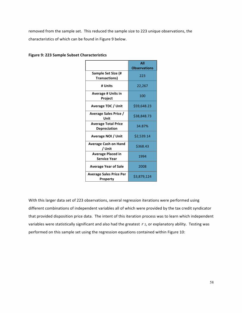
58
removed from the sample set. This reduced the sample size to 223 unique observations, the
characteristics of which can be found in Figure 9 below.
Figure 9: 223 Sample Subset Characteristics
All Observations
Sample Set Size (# Transactions) 223
# Units 22,267
Average # Units in Project
100
Average TDC / Unit $59,648.23
Average Sales Price / Unit $38,848.73
Average Total Price Depreciation 34.87%
Average NOI / Unit $2,539.14
Average Cash on Hand / Unit $368.43
Average Placed in Service Year 1994
Average Year of Sale 2008
Average Sales Price Per Property
$3,879,124
With this larger data set of 223 observations, several regression iterations were performed using
different combinations of independent variables all of which were provided by the tax credit syndicator
that provided disposition price data. The intent of this iteration process was to learn which independent
variables were statistically significant and also had the greatest r 2, or explanatory ability. Testing was
performed on this sample set using the regression equations contained within Figure 10:
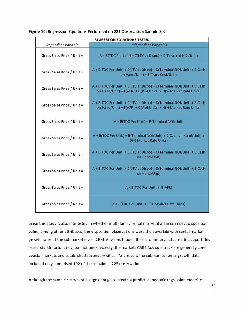
59
Figure 10: Regression Equations Performed on 223 Observation Sample Set
REGRESSION EQUATIONS TESTED Dependent Variable Independent Variables
Gross Sales Price / Unit = A + B(TDC Per Unit) + C(LTV at Dispo) + D(Terminal NOI/Unit)
Gross Sales Price / Unit = A + B(TDC Per Unit) + C(LTV at Dispo) + D(Terminal NOI/Unit) + E(Cash
on Hand/Unit) + F(Tran. Cost/Unit)
Gross Sales Price / Unit = A + B(TDC Per Unit) + C(LTV at Dispo) + D(Terminal NOI/Unit) + E(Cash on Hand/Unit) + F(AFR) + G(# of Units) + H(% Market Rate Units)
Gross Sales Price / Unit = A + B(TDC Per Unit) + C(LTV at Dispo) + D(Terminal NOI/Unit) + E(Cash
on Hand/Unit) + F(AFR) + G(# of Units) + H(% Market Rate Units)
Gross Sales Price / Unit = A + B(TDC Per Unit) + B(Terminal NOI/Unit)
Gross Sales Price / Unit = A + B(TDC Per Unit) + B(Terminal NOI/Unit) + C(Cash on Hand/Unit) +
D(% Market Rate Units)
Gross Sales Price / Unit = A + B(TDC Per Unit) + C(LTV at Dispo) + D(Terminal NOI/Unit) + E(Cash on Hand/Unit)
Gross Sales Price / Unit = A + B(TDC Per Unit) + C(LTV at Dispo) + D(Terminal NOI/Unit) + E(Cash on Hand/Unit)
Gross Sales Price / Unit = A + B(TDC Per Unit) + B(AFR)
Gross Sales Price / Unit = A + B(TDC Per Unit) + C(% Market Rate Units)
Since this study is also interested in whether multi-‐family rental market dynamics impact disposition
value, among other attributes, the disposition observations were then overlaid with rental market
growth rates at the submarket level. CBRE Advisors tapped their proprietary database to support this
research. Unfortunately, but not unexpectedly, the markets CBRE Advisors track are generally core
coastal markets and established secondary cities. As a result, the submarket rental growth data
included only comprised 102 of the remaining 223 observations.
Although the sample set was still large enough to create a predictive hedonic regression model, of

60
course additional observations would contribute to a more comprehensive and defensible model. An
alternative observable variable that was indicative intuitively of the strength of the rental market was
sought to add back observations for analysis. Publicly available U.S. Census data on job growth rates at
the MSA level in the year of disposition was gathered to meet this need and provide an alternative
sample subset for analysis. Although the sample included some rural observations not included in the
MSA level job growth data, job growth rates in the year of disposition were available for 211 of the 223-‐
observation sample set. This sample subset was used as a larger alternative to the rental growth subset
and was tested for predictability using hedonic regression.
A series of regressions were run on both sample subsets. None of the regression results presented an
r 2 that exceeded .50, which is the threshold used in this study for considering a model adequately
predictive to provide conclusions from the data within the range of the sample set. Raw data was
scrubbed to consider whether there were any outliers in the sample set. The methodology for mining
outliers was to compare the TDC per unit data points to the corresponding Gross Sales Price per unit
data points. Any observations that were inconsistent with the broader sample were considered
outliers. The general correlation line between these data points depicts an upward sloping linear
correlation with a higher TDC corresponding to a higher Gross Sales Price. Predictably, in almost all
cases, the physical depreciation over the 15-‐year Initial Compliance Period leads to a significantly lower
disposition price than the original TDC. The relationship can be seen graphically in Figure 11 below.

61
Figure 11: Linear Correlation – TDC / Unit to Sales Price / Unit
Through this analysis, two outliers were identified and removed from both the Rent Growth and Job
Growth data sets. This vastly improved the r 2 calculation of both regression models, but upon further
review, the inclusion of the LTV at Disposition independent variable as a joint causal and partially
truncated predictive variable was observed. Although the amount of the outstanding debt is extremely
predictive of sales price, since many dispositions have appraised values that are less than the
outstanding debt, the observed Gross Sales Price defaults to the amount of the outstanding debt. The
limits to the LTV at Disposition as a useful predictive variable can be seen graphically below in Figure 12,
where the corresponding disposition value truncates at LTVs that approach 1.0.
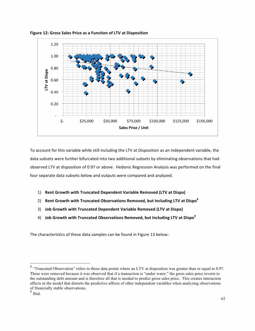
62
Figure 12: Gross Sales Price as a Function of LTV at Disposition
To account for this variable while still including the LTV at Disposition as an independent variable, the
data subsets were further bifurcated into two additional subsets by eliminating observations that had
observed LTV at disposition of 0.97 or above. Hedonic Regression Analysis was performed on the final
four separate data subsets below and outputs were compared and analyzed.
1) Rent Growth with Truncated Dependent Variable Removed (LTV at Dispo)
2) Rent Growth with Truncated Observations Removed, but Including LTV at Dispo8
3) Job Growth with Truncated Dependent Variable Removed (LTV at Dispo)
4) Job Growth with Truncated Observations Removed, but Including LTV at Dispo9
The characteristics of these data samples can be found in Figure 13 below:
8 “Truncated Observation” refers to those data points where an LTV at disposition was greater than or equal to 0.97. These were removed because it was observed that if a transaction is “under water,” the gross sales price reverts to the outstanding debt amount and is therefore all that is needed to predict gross sales price. This creates interaction affects in the model that distorts the predictive affects of other independent variables when analyzing observations of financially stable observations. 9 Ibid.
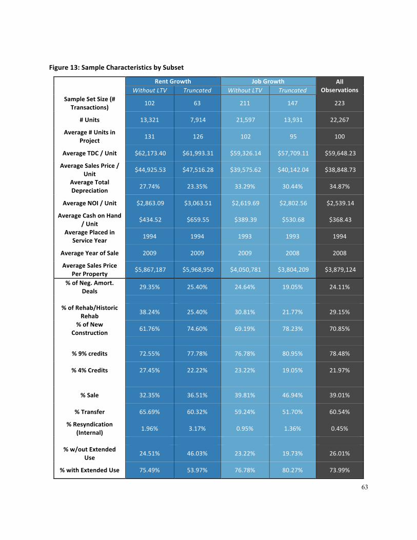
63
Figure 13: Sample Characteristics by Subset
Rent Growth Job Growth All Observations Without LTV Truncated Without LTV Truncated
Sample Set Size (# Transactions)
102 63 211 147 223
# Units 13,321 7,914 21,597 13,931 22,267
Average # Units in Project 131 126 102 95 100
Average TDC / Unit $62,173.40 $61,993.31 $59,326.14 $57,709.11 $59,648.23
Average Sales Price / Unit
$44,925.53 $47,516.28 $39,575.62 $40,142.04 $38,848.73
Average Total Depreciation 27.74% 23.35% 33.29% 30.44% 34.87%
Average NOI / Unit $2,863.09 $3,063.51 $2,619.69 $2,802.56 $2,539.14
Average Cash on Hand / Unit
$434.52 $659.55 $389.39 $530.68 $368.43
Average Placed in Service Year 1994 1994 1993 1993 1994
Average Year of Sale 2009 2009 2009 2008 2008
Average Sales Price Per Property
$5,867,187 $5,968,950 $4,050,781 $3,804,209 $3,879,124
% of Neg. Amort. Deals
29.35% 25.40% 24.64% 19.05% 24.11%
% of Rehab/Historic
Rehab 38.24% 25.40% 30.81% 21.77% 29.15%
% of New Construction 61.76% 74.60% 69.19% 78.23% 70.85%
% 9% credits 72.55% 77.78% 76.78% 80.95% 78.48%
% 4% Credits 27.45% 22.22% 23.22% 19.05% 21.97%
% Sale 32.35% 36.51% 39.81% 46.94% 39.01%
% Transfer 65.69% 60.32% 59.24% 51.70% 60.54%
% Resyndication (Internal) 1.96% 3.17% 0.95% 1.36% 0.45%
% w/out Extended
Use 24.51% 46.03% 23.22% 19.73% 26.01%
% with Extended Use 75.49% 53.97% 76.78% 80.27% 73.99%
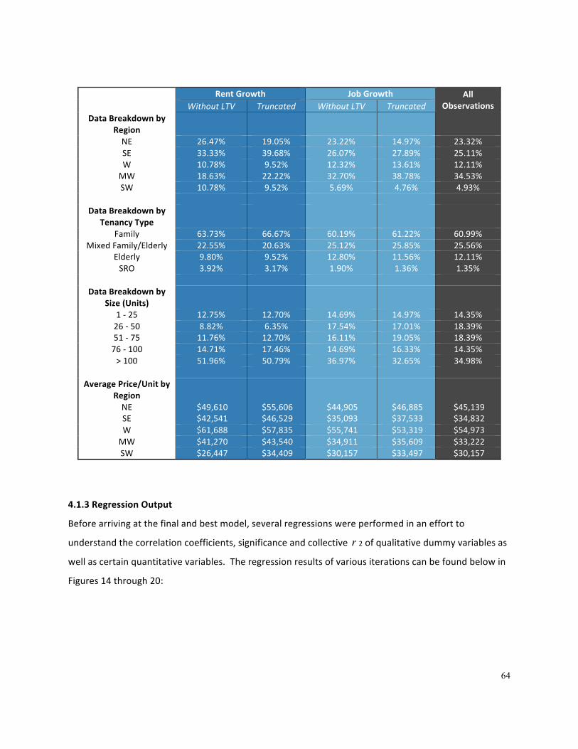
64
Rent Growth Job Growth All Observations Without LTV Truncated Without LTV Truncated
Data Breakdown by Region
NE 26.47% 19.05% 23.22% 14.97% 23.32% SE 33.33% 39.68% 26.07% 27.89% 25.11% W 10.78% 9.52% 12.32% 13.61% 12.11% MW 18.63% 22.22% 32.70% 38.78% 34.53% SW 10.78% 9.52% 5.69% 4.76% 4.93%
Data Breakdown by Tenancy Type
Family 63.73% 66.67% 60.19% 61.22% 60.99% Mixed Family/Elderly 22.55% 20.63% 25.12% 25.85% 25.56%
Elderly 9.80% 9.52% 12.80% 11.56% 12.11% SRO 3.92% 3.17% 1.90% 1.36% 1.35%
Data Breakdown by Size (Units)
1 -‐ 25 12.75% 12.70% 14.69% 14.97% 14.35% 26 -‐ 50 8.82% 6.35% 17.54% 17.01% 18.39% 51 -‐ 75 11.76% 12.70% 16.11% 19.05% 18.39% 76 -‐ 100 14.71% 17.46% 14.69% 16.33% 14.35% > 100 51.96% 50.79% 36.97% 32.65% 34.98%
Average Price/Unit by
Region
NE $49,610 $55,606 $44,905 $46,885 $45,139 SE $42,541 $46,529 $35,093 $37,533 $34,832 W $61,688 $57,835 $55,741 $53,319 $54,973 MW $41,270 $43,540 $34,911 $35,609 $33,222 SW $26,447 $34,409 $30,157 $33,497 $30,157
4.1.3 Regression Output
Before arriving at the final and best model, several regressions were performed in an effort to
understand the correlation coefficients, significance and collective r 2 of qualitative dummy variables as
well as certain quantitative variables. The regression results of various iterations can be found below in
Figures 14 through 20:
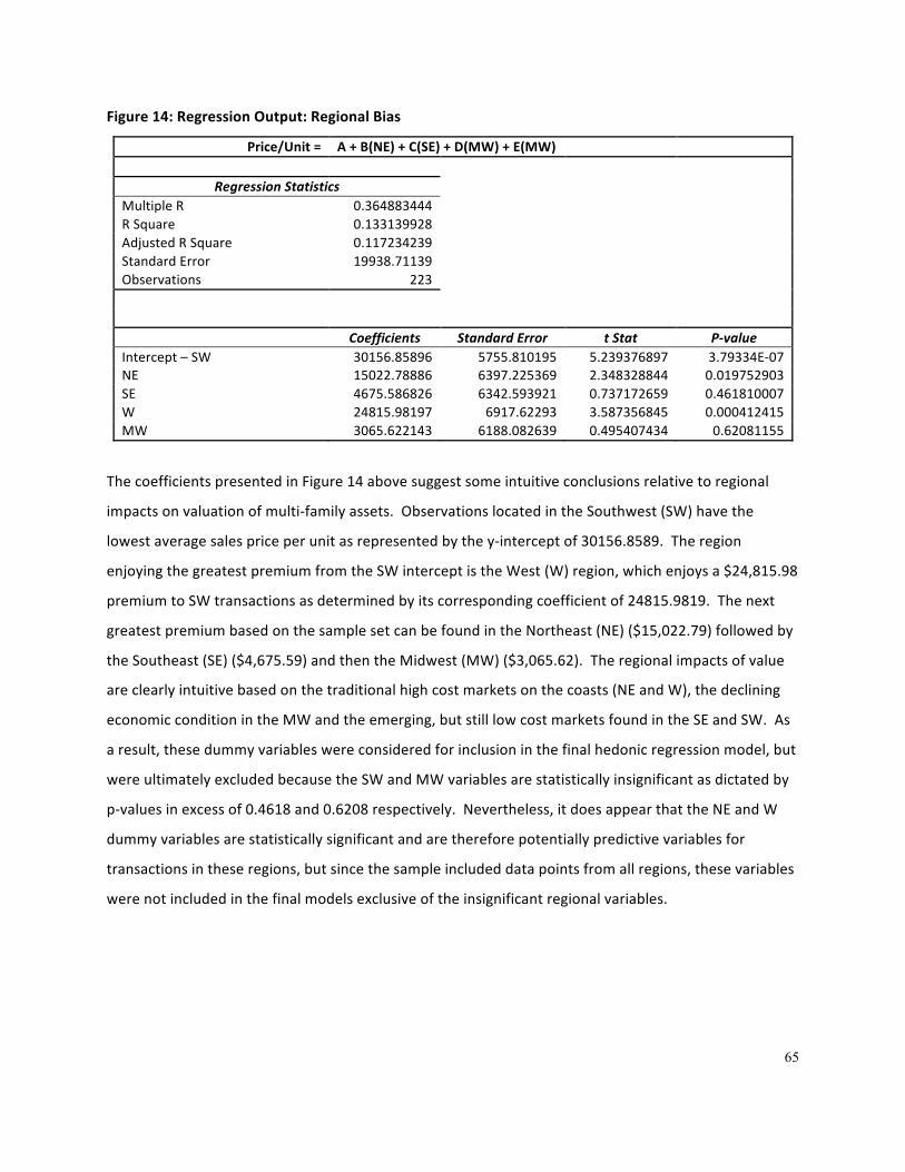
65
Figure 14: Regression Output: Regional Bias
Price/Unit = A + B(NE) + C(SE) + D(MW) + E(MW)
Regression Statistics Multiple R 0.364883444 R Square 0.133139928 Adjusted R Square 0.117234239 Standard Error 19938.71139 Observations 223
Coefficients Standard Error t Stat P-‐value Intercept – SW 30156.85896 5755.810195 5.239376897 3.79334E-‐07 NE 15022.78886 6397.225369 2.348328844 0.019752903 SE 4675.586826 6342.593921 0.737172659 0.461810007 W 24815.98197 6917.62293 3.587356845 0.000412415 MW 3065.622143 6188.082639 0.495407434 0.62081155
The coefficients presented in Figure 14 above suggest some intuitive conclusions relative to regional
impacts on valuation of multi-‐family assets. Observations located in the Southwest (SW) have the
lowest average sales price per unit as represented by the y-‐intercept of 30156.8589. The region
enjoying the greatest premium from the SW intercept is the West (W) region, which enjoys a $24,815.98
premium to SW transactions as determined by its corresponding coefficient of 24815.9819. The next
greatest premium based on the sample set can be found in the Northeast (NE) ($15,022.79) followed by
the Southeast (SE) ($4,675.59) and then the Midwest (MW) ($3,065.62). The regional impacts of value
are clearly intuitive based on the traditional high cost markets on the coasts (NE and W), the declining
economic condition in the MW and the emerging, but still low cost markets found in the SE and SW. As
a result, these dummy variables were considered for inclusion in the final hedonic regression model, but
were ultimately excluded because the SW and MW variables are statistically insignificant as dictated by
p-‐values in excess of 0.4618 and 0.6208 respectively. Nevertheless, it does appear that the NE and W
dummy variables are statistically significant and are therefore potentially predictive variables for
transactions in these regions, but since the sample included data points from all regions, these variables
were not included in the final models exclusive of the insignificant regional variables.

66
Figure 15: Regression Output: Construction Type Bias
Price/Unit = A + B(New) + C(Rehab)
Regression Statistics Multiple R 0.125242113 R Square 0.015685587 Adjusted R Square 0.006737274 Standard Error 21149.80736 Observations 223
Coefficients Standard Error t Stat P-‐value Intercept -‐ Historic Rehab 47115.08098 4729.240696 9.962504344 1.55443E-‐19 New -‐9395.886201 5021.439391 -‐1.87115396 0.062651192 Rehab -‐8096.73618 5664.798548 -‐1.429306993 0.154334429
The intuition on testing this variable related to the literature, which suggests that many early era LIHTC
transactions were done via “light” rehabilitations meaning that minimal rehabilitation scope was
performed. A negative bias toward rehabs was expected as a result, with these transactions trading at a
discount due to poor physical condition or deferred capital improvement needs. A discount was also
expected due to the years from the original construction, which would contribute to smaller unit
configurations and outdated unit and property amenities. As dictated by the coefficients in Figure 15
above, the Historic Rehab properties enjoy the highest disposition price per unit in the sample. This is
surprising, but could perhaps be explained by the fact that Historic Rehabs receive additional Federal
Historic Tax Credits in conjunction with LIHTCs as a part of their original capital structure to compensate
for the high cost of historic restoration. This typically results in the original TDC per unit being higher
than comparable rehab and new construction projects, which clearly has a huge impact on what the
property sells for at the end of the Initial Compliance Period. Surprisingly, the New Construction
projects in the sample show a greater discount per unit (-‐ $9,395.88) to the Historic Rehabs than
conventional Rehabs (-‐ $8,096.74). There is no logical explanation for this other than randomness. In
addition, neither the New Construction variable nor the Rehab variable are statistically significant based
on their respective p-‐values. As a result these dummy variables were left out of the final models.
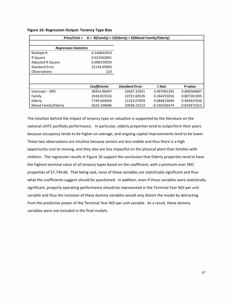
67
Figure 16: Regression Output: Tenancy Type Bias
Price/Unit = A + B(Family) + C(Elderly) + D(Mixed Family/Elderly)
Regression Statistics Multiple R 0.146842914 R Square 0.021562841 Adjusted R Square 0.008159593 Standard Error 21134.65903 Observations 223
Coefficients Standard Error t Stat P-‐value Intercept – SRO 36953.96497 10567.32951 3.497001293 0.000569607 Family 2618.815516 10721.60526 0.244255916 0.807261305 Elderly 7749.664004 11323.07059 0.684413644 0.494437636 Mixed Family/Elderly -‐2626.338686 10938.22523 -‐0.240106474 0.810472313
The intuition behind the impact of tenancy type on valuation is supported by the literature on the
national LIHTC portfolio performance. In particular, elderly properties tend to outperform their peers
because occupancy tends to be higher on average, and ongoing capital improvements tend to be lower.
These two observations are intuitive because seniors are less mobile and thus there is a high
opportunity cost to moving, and they also are less impactful on the physical plant than families with
children. The regression results in Figure 16 support the conclusion that Elderly properties tend to have
the highest terminal value of all tenancy types based on the coefficient, with a premium over SRO
properties of $7,749.66. That being said, none of these variables are statistically significant and thus
what the coefficients suggest should be questioned. In addition, even if these variables were statistically
significant, property operating performance should be represented in the Terminal Year NOI per unit
variable and thus the inclusion of these dummy variables would only distort the model by detracting
from the predictive power of the Terminal Year NOI per unit variable. As a result, these dummy
variables were not included in the final models.

68
Figure 17: Regression Output: Disposition Type Bias
Price/Unit = A + B(Sale) + C(Transfer)
Regression Statistics Multiple R 0.104408678 R Square 0.010901172 Adjusted R Square 0.001909364 Standard Error 21201.14603 Observations 223
Coefficients Standard Error t Stat P-‐value Intercept -‐ Resyndication 55025.92949 14991.47413 3.67048157 0.000303854 Sale -‐14347.3384 15164.79172 -‐0.946095315 0.345137933 Transfer -‐17613.71935 15102.11381 -‐1.166308212 0.244752621
The intuition in testing this qualitative attribute was that sales would command a higher price than
transfers as transfers are typically done when the value of the property is less than the outstanding
debt. As discussed previously, Syndicators view these properties as liabilities and typically try to harvest
tax benefits through a transfer of the asset to the GP. Resyndication is referring to the recapitalization
of the Year 15 transaction with a new LIHTC allocation, which was purchased or “resyndicated” by the
syndicator who provided the sample set. Abt Associates study and logic support that a resyndication
typically results in greater sales proceeds of the Year 15 property because the new financing can support
significant acquisition cost. It is important to note that less than one percent of the observations in the
sample set were resyndications, but nevertheless, based on the regression results, this practice yields a
significantly higher disposition value. Transfers show the deepest discount to resyndications coming in
at -‐$17,613.72, with Sales only slightly better at -‐$14,347.34. Despite the intuitive nature of the
coefficients, these variables also lack statistical significance and were therefore excluded from the final
models. There is also a joint causal issue with these variables as the sale type is likely triggered by the
terminal value relative to outstanding debt at disposition versus the type of sale impacting the gross
sales proceeds.
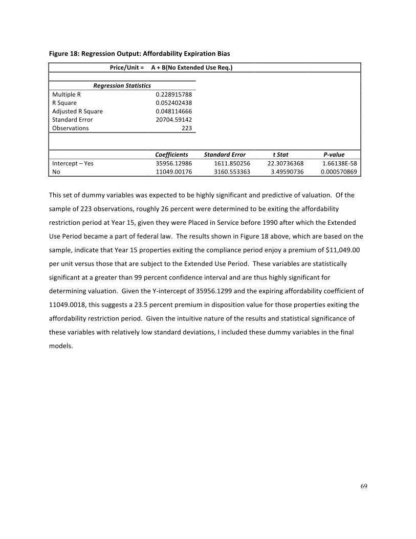
69
Figure 18: Regression Output: Affordability Expiration Bias
Price/Unit = A + B(No Extended Use Req.)
Regression Statistics Multiple R 0.228915788 R Square 0.052402438 Adjusted R Square 0.048114666 Standard Error 20704.59142 Observations 223
Coefficients Standard Error t Stat P-‐value Intercept – Yes 35956.12986 1611.850256 22.30736368 1.66138E-‐58 No 11049.00176 3160.553363 3.49590736 0.000570869
This set of dummy variables was expected to be highly significant and predictive of valuation. Of the
sample of 223 observations, roughly 26 percent were determined to be exiting the affordability
restriction period at Year 15, given they were Placed in Service before 1990 after which the Extended
Use Period became a part of federal law. The results shown in Figure 18 above, which are based on the
sample, indicate that Year 15 properties exiting the compliance period enjoy a premium of $11,049.00
per unit versus those that are subject to the Extended Use Period. These variables are statistically
significant at a greater than 99 percent confidence interval and are thus highly significant for
determining valuation. Given the Y-‐intercept of 35956.1299 and the expiring affordability coefficient of
11049.0018, this suggests a 23.5 percent premium in disposition value for those properties exiting the
affordability restriction period. Given the intuitive nature of the results and statistical significance of
these variables with relatively low standard deviations, I included these dummy variables in the final
models.

70
In addition dummy variable testing for qualitative variables that were expected to impact value, several
quantitative variables were analyzed using correlation scatter plots to determine suitability for inclusion
in the final models.
Figure 19: Correlation Scatter Plot: Project Size (# units)
Although the fitted regression line in Figure 19 above suggests a negative relationship between Project
Size by number of units and gross sales price, there is a great deal of dispersion in the data points, so the
line should not be considered indicative of a strong linear relationship between the variables. As the
graph indicates, the line suggests that as projects get smaller on a per unit basis, the disposition price
per unit goes up. This relationship is certainly contrary to the intuition that a premium would be paid on
a per unit basis for larger properties given their institutional size and thus greater attractiveness to a
wider array of buyers. The scatter plot shows that a linear relationship is lacking between these
variables and regression models tested including this independent variable also support its lack of
statistical significance. As a result, this data point was excluded as a variable in the final models.

71
Figure 20: Correlation Scatter Plot: Year of Sale
The Year of Sale variable was correlated against Gross Sales Price to see whether there was a linear
relationship with disposition proceeds. This was done to account for any potential macroeconomic price
bias given the real estate cycle(s) from 2004 – 2012. Although date of sale is a continuous variable, by
simplifying this variable to the Year of Sale, it becomes a discrete variable. As you can see from the
graph in Figure 20, this creates a graph that resembles a histogram, which shows variation in sale price
on the x-‐axis based on the discrete Year of Sale on the y-‐axis. The regression line should be completely
ignored in this scatter plot as it merely represents the average year of disposition for the sample set. It
is clear from the scatter plot and regression results that wide dispersion exists in sales proceeds by year
of disposition with no discernable pattern. As a result, this variable was excluded from the final models.
With results from various linear regression and scatter plots in hand, it was clear that the only
qualitative variable that was statistically significant and had clear explanatory qualities for disposition
price was the affordability expiration dummy variable. This was included along with intuitively impactful
quantitative variables such as the original TDC of the project, the Terminal Year NOI, the Terminal Year
Cash Balance including reserves and the submarket Rental Growth Rate. Regressions were run on the
Rent Growth and Job Growth sample subsets as described above and results were as follows:

72
Figure 21: Regression Output: Rent Growth Subset
The results for the best and most predictive model appear in Figure 21 above. The results are included
here along with other hedonic model regression results as a means of comparison to help to illustrate
why this is the most predictive model based on the analysis of the data and regression methodology.
This model achieves the highest r 2 , as compared to the three other models below, which indicates that
it has the most explanatory power of all of the models. In addition, the sign and magnitude of
coefficients for respective variables are logical and consistent with previously generated regression and
correlation tests. All variables are significant at a confidence interval of greater than 99 percent with the
exception of the Rental Growth Rate in the year of disposition variable, which is statistically significant at
greater than a 95 percent confidence interval. At a most basic level, this model indicates that the
terminal value of a Year 15 LIHTC property can be reasonably estimated and is a function of its original
TDC, the NOI at Year 15, the property Cash on Hand, the terminal year submarket Rental Growth Rate in
which it is located and whether or not requirements to maintain the property as Affordable Housing are
expiring. A granular analysis of the most predictive model results along with policy implications can be
found in Chapter 5.
Price/Unit = A + B(TDC Per Unit) + C(Terminal NOI/Unit) + D(Cash on Hand/Unit) + E(Rent Gr. Yr. of Dispo)
+ F(Affordability Expiration)
Regression Statistics Multiple R 0.789718959 R Square 0.623656034 Adjusted R Square 0.604054785 Standard Error 14989.8176 Observations 102
Coefficients Standard Error t Stat P-‐value Intercept 3468.828352 3900.805047 0.889259604 0.376086493 Total Development Cost / Unit 0.411157803 0.059308838 6.93248788 4.77122E-‐10 Terminal Year NOI / Unit 3.510918155 0.845971756 4.150160015 7.18836E-‐05 Reserves/Cash Balance / Unit 3.914169696 1.340052966 2.920906708 0.004350302 Rent Growth Yr. of Dispo (%) 813.5412327 402.4950062 2.021245531 0.046038601 Affordability Expiration 10517.16037 3603.540545 2.918563074 0.004380412

73
Figure 22: Regression Output: Rent Growth Subset with Truncated Observations Removed
Price/Unit = A + B(TDC Per Unit) + C(Terminal NOI/Unit) + D(Cash on Hand/Unit) + E(Rent Gr. Yr. of Dispo) + F(Affordability Expiration) + G(LTV at Dispo)
Regression Statistics Multiple R 0.811741475 R Square 0.658924222 Adjusted R Square 0.622380388 Standard Error 15147.16403 Observations 63
Coefficients Standard Error t Stat P-‐value Intercept 16959.24184 12263.31407 1.382924856 0.172177531 Total Development Cost / Unit 0.497194484 0.103728305 4.793238306 1.24987E-‐05 Terminal Year NOI / Unit 1.547066375 1.405302713 1.100877669 0.27565947 Reserves/Cash Balance / Unit 3.770175224 1.588522254 2.37338521 0.021082021 Rent Growth Yr. of Dispo (%) 1502.917334 609.7314264 2.464884159 0.016798595 Affordability Expiration 9912.032857 5002.651958 1.981355677 0.052469252 LTV at Time of Dispo -‐15856.57032 15873.05299 -‐0.998961594 0.322110399
The model depicted in Figure 22 above was created in an attempt to include the LTV at Disposition
variable within the model by removing all observations that had an LTV at disposition of 0.97 or above.
Since the LTV at Disposition variable is truncated as described in Section 1.3, the theory is that those
observations with LTV ratios close to “1.0” were likely valued at an amount that was far less than the
outstanding principal balance of debt, but the transfer or sale price reverted to the amount of
outstanding debt since a LIHTC property cannot trade for an amount that is less than the debt balance.
By removing those observations that were overleveraged, the expectation was that a more predictive
model would be created and the LTV ratio could then be included as a predictive variable for disposition
value. As you can see from the regression results, adding the LTV at Disposition independent variable on
this sample subset made the Terminal Year NOI per unit variable statistically insignificant while the LTV
at Disposition variable remained statistically insignificant as discovered in previous regression iterations.
The increase in the explanatory power of this model versus the previous model as exhibited by a higher
r 2 should therefore be discounted along with the usefulness of this model.

74
Figure 23: Regression Output: Job Growth Subset
Price/Unit = A + B(TDC Per Unit) + C(Terminal NOI/Unit) + D(Cash on Hand/Unit) + E(Job Gr. Yr. of Dispo) + F(Affordability Expiration)
Regression Statistics Multiple R 0.736559712 R Square 0.542520209 Adjusted R Square 0.531362166 Standard Error 14523.51759 Observations 211
Coefficients Standard Error t Stat P-‐value Intercept 2634.487549 2707.828398 0.972915252 0.331742007 Total Development Cost / Unit 0.387286759 0.041256007 9.387402991 1.21302E-‐17 Terminal Year NOI / Unit 3.737263903 0.563463146 6.632667861 2.87324E-‐10 Reserves/Cash Balance / Unit 3.836814843 0.880241895 4.358818713 2.06778E-‐05 Job Growth Yr. of Sale (%) 140.6570888 390.0412824 0.36062103 0.718754079 Affordability Expiration 11434.6524 2402.773821 4.758938316 3.67033E-‐06
Job Growth Rate in the year of disposition was substituted for Rent Growth Rate in this model. This
added more than double the sample set from the Rent Growth subset (from 103 to 211 observations)
allowing for a much larger and less biased sample set. Aside from this modification, the model remains
unchanged from the model illustrated in Figure 21. The regression results, which appear in Figure 23
above, indicate that the Job Growth Rate in the year of disposition in the MSA in which the property is
located is statistically insignificant. In addition, the r 2 dropped significantly in this model suggesting that
using this variable and taking into account the larger sample set reveals a model that is only useful for
predicting a little more than 54 percent of the total variation of outcomes explained by the model.
Clearly the Job Growth Rate and the Rental Growth Rate in a particular MSA are not necessarily directly
correlated. The presence of a lag between the data points is also likely since job growth is sometimes a
leading indicator for rent growth in many submarkets. Another possible explanation for the rent growth
rate’s usefulness as a predictive variable lies in the urban bias of the Rent Growth subset versus the Job
Growth subset. As previously discussed, Abt Associates’ recent study notes that the impact on Year 15
valuation by the strength of the rental submarket is more pronounced in urban and high cost
submarkets where prevailing market rents are significantly higher than the maximum LIHTC rents
allowed under the program guidelines. In rural and smaller MSA submarkets where LIHTC rents
approximate fair market rents, the ability to raise rents provides zero benefit to the owner because the

75
market will not support higher rents. In order to test whether the urban bias in the Rent Growth subset
was revealing the Rental Growth Rate at disposition as statistically significant when it would in fact not
be if the same data was available for rural and smaller MSAs, a correlation scatter plot was created
comparing the Rental Growth Rate data points for the Rent Growth sample subset against the Job
Growth Rate numbers for the same sample subset. The scatter plot appears below in Figure 24:
Figure 24: Correlation Scatter Plot: Rental Growth Rates vs. Job Growth Rates for Rent Growth Subset
Figure 24 indicates a strong positive correlation between Rental Growth Rate and Job Growth Rate for
the Rent Growth sample subset indicating that there may be truth to the notion that the urban and
larger MSA bias of the Rent Growth subset is influencing the statistical significance of the strength of the
Rental Growth Rate as a predictor of terminal valuation. If the model were applied to a larger subset
that included more rural and smaller MSA observations, the strength of the rental market may not be as
useful for predicting terminal valuation.

76
Figure 25: Regression Output: Job Growth Subset Truncated Observations Removed
Price/Unit = A + B(TDC Per Unit) + C(Terminal NOI/Unit) + D(Cash on Hand/Unit) + E(Job Gr. Yr. of Dispo) + F(Affordability Expiration)+ G(LTV at Dispo)
Regression Statistics Multiple R 0.742570293 R Square 0.551410641 Adjusted R Square 0.532185382 Standard Error 15003.47019 Observations 147
Coefficients Standard Error t Stat P-‐value Intercept 14988.0169 6394.929354 2.343734554 0.020498681 Total Development Cost / Unit 0.429411878 0.056530354 7.59612927 3.95089E-‐12 Terminal Year NOI / Unit 3.369078022 0.771634375 4.366158547 2.44177E-‐05 Reserves/Cash Balance / Unit 3.370137772 0.967995593 3.481563134 0.000665274 Job Growth Yr. of Sale (%) 211.4502494 457.9851054 0.461696782 0.645015373 Affordability Expiration 8238.542902 3203.773828 2.571512018 0.011168494 LTV at Dispo -‐17433.26433 6934.763152 -‐2.5138947 0.013072829
The regression results found in Figure 25 above were produced using the same model as results found in
Figure 22, but applied to the Job Growth sample subset and substituting the Job Growth Rate at
disposition variable for the Rental Growth Rate at disposition variable. As compared to the similar Rent
Growth model, the LTV at Disposition variable now appears statistically significant and the coefficient
for this variable indicates a great negative influence on valuation. The Job Growth Rate at disposition
remains statistically insignificant in this model and the r 2 remains below that of the Rent Growth
sample subset.
4.1.4 Hedonic Pricing Model
It is clear from the regression output that the best hedonic regression equation for predicting the
terminal year valuation based on the provided sample is as follows:
Price/Unit = 3468.83 + 0.41(TDC Per Unit) + 3.51(Terminal NOI/Unit) + 3.91(Cash on Hand/Unit) + 813.54(Rent Gr. Yr. of Dispo) + 10517.16(Affordability Expiration)
This equation can be used to estimate terminal year valuation with a high degree of confidence and the
variables included provide a coefficient of determination ( r 2) for the overall model of 0.6237. The

77
coefficient of determination is found by dividing the regression sum of squares (the amount of variation
or squared deviations in the observed value of the response variable or Gross Sales Price per unit) by the
total sum of squares (the total variation in the observed values of the response variable) (Weiss, Neil,
2008). The r 2 measures the usefulness of the regression equation in making accurate predictions of
price and is always between 0 and 1. An r 2 of 0.6237 suggests the model is useful in making predictions
as it explains 62 percent of the variation in price, but also indicates a strong element of randomness
associated with the pricing of Year 15 LIHTC transactions.
4.2 Strengths & Weaknesses of Methodology
The strength of the chosen methodology is in the quality of the provided data sources as well as the use
of hedonic regression analysis, which is a widely respected and highly effective statistical analysis tool
for drawing empirical conclusions from pricing observations. Since data was provided by two very
reliable proprietary sources, the data analyzed to create the regression model should be extremely
accurate. In addition, the broad array of provided transaction level data allowed for an analysis of an
array of variables to discern impact on observed disposition prices. The quality of the data makes it
very likely that the model provides an accurate picture of the factors which impact Year 15 valuation in
LIHTC transactions. The methodology, however, is not without limitations.
The main weakness in the methodology is the lack of availability of more observations and the lack of
diversity in the source of such observations. Given the relative youth of the LIHTC program, Year 15
observations could only be tracked beginning in 2001. Although this provides more than a decade of
observations industry-‐wide, as previously mentioned, many of these transactions included HUD section
515 loans, which are no longer paired with the LIHTC and are therefore not applicable for understanding
what will impact valuation of Year 15 transactions in the future. This practice was largely abandoned by
1990, so the observations that would be useful to this analysis, which are available industry-‐wide, begin
with 2005-‐era dispositions. More than seven years of observations industry-‐wide is significant, but since
only one syndicator supported this study, only a fraction of available observations were included in this
analysis. This was exacerbated by the large quantity of rural transactions for which submarket level rent
growth data was unavailable. The study conclusions would be far stronger if the same study was
conducted using a larger sample set as opposed to what is estimated to be less than five percent of the
78
disposition data available industry-‐wide.10 With the existing sample set, the model and corresponding
conclusions lack depth, due to the small size.
The single source of data also makes the data subject to a Syndicator specific bias. This bias could stem
from the form of limited partnership agreement governing the disposition process among other
transaction level functions, which usually remains more or less consistent in form across a Syndicator’s
portfolio of Lower Tier transactions. Legal rights and obligations contained in LPAs should be relatively
standardized across the industry, but it is likely that significant differences do exist among syndicator
preferences for the handling of the Year 15 disposition process given specific investor’s differing
motivations. Thus the presence of a corresponding bias in this study’s conclusions is possible. It is
important to note that despite the sole source of the data, the regional location, construction type and
tenancy type, among other attributes are highly diverse and therefore representative of the broader
national LIHTC portfolio.
Another weakness in the methodology is the lack of rental growth rate detail available for transactions
outside of larger MSAs. In an effort to understand the impact of the multi-‐family rental market on
valuation, the sample set was paired down to those observations for which submarket rental growth
data was available. As a result, the study conclusions have both an urban and larger MSA bias that may
eliminate nuances in the data. For example, it is likely and hypothesized in literature that the strength
of the underlying rental market has less impact on Year 15 valuation in more rural areas because of a
lack of long-‐term growth prospects and less interest from ILP interest buyers and thus a lack of liquidity
in the market for Year 15 ILP interests (Abt Associates, 2012). The lack of a discernable difference
between prevailing fair market rents and the maximum LIHTC rents that is more common in rural and
smaller MSAs also results in less impact on valuation for those properties exiting the affordability period
as discussed in section 4.1.3 above. The impact of the rental market on Year 15 transactions industry-‐
wide should therefore be questioned without repeating this study on a larger sample set that includes
observations in rural and smaller MSA submarkets.
10 Estimate based on Abt Associates’ estimate of properties reaching Year 15 through 2009.

79
Chapter 5
Data Analysis & Interpretation
5.1 Predicted Outcomes of Data Set
The overarching intuition regarding Year 15 prior to undertaking this research and analysis was that
valuation was largely unaffected by characteristics and attributes that typically affect conventionally
financed market rate multi-‐family transactions. This was hypothesized given the Extended Use Period
that most Year 15 transactions would be subject to, but also because of complex financial structures
that create a lack of a secondary market for ILP interests and thus a lack of liquidity. An inefficient
market that was not taking into account the true value of ILP interests based on market fundamentals
was expected. In addition, linear relationships between several transaction level quantitative and
qualitative attributes were expected. Among the quantitative attributes, it was expected that the layers
of soft debt common in LIHTC transactions would be highly predictive of valuation as dictated by the
terminal year LTV and that the project size in units, the original TDC, terminal year NOI and cash on hand
would also be significant drivers of value. On the qualitative side, region, construction type, tenancy and
affordability period expiration were all expected to impact valuation with some statistical significance,
though to a lesser degree than the qualitative transactional attributes. The regression results from the
subject sample set mostly support conclusions about Year 15 dynamics found in previous literature, but
the creation of a predictive model that can be used to help the industry understand what impacts the
value of Year 15 transactions is a new addition to the industry’s understanding of Year 15.
5.2 Interpretation of the Model
Price/Unit = 3468.83 + 0.41(TDC Per Unit) + 3.51(Terminal NOI/Unit) + 3.91(Cash on Hand/Unit) + 813.54(Rent Gr. Yr. of Dispo) + 10517.16(Affordability Expiration)
The most predictive variables for determining the Gross Sale Price at disposition on or around Year 15 as
dictated by this model are the original TDC of the project, the Terminal Year NOI, the Terminal Year Cash
Balance including reserves, whether the project is subject to the extended use Affordability Period and
the submarket Rental Growth Rate. These variables are able to account for 62 percent of the overall
sale price as determined by the r 2 in the model of .6236.

80
The Rental Growth Rate variable is only significant at a 96.4 percent confidence interval, while all other
variables are significant at a 99.99 percent confidence level. At a basic level, the estimated coefficients
on disposition observation characteristics (independent variables) may be interpreted as an implicit
price that buyers are willing to pay for more of each attribute (Wheaton and DiPasquale, 1996).
The greatest incremental impact on sale price as determined by the correlation coefficient can be found
with the Affordability Expiration dummy variable. The coefficient of 10517.1604 indicates that projects
exiting the compliance period that are not subject to the Extended Use Period enjoy a sale price
premium of approximately $10,517 per unit. As compared to the average observed sale price of the
sample set of $44,925 per unit, this represents a significant premium on a percentage basis of the total
price. The price premium suggests that the buyer intends to reposition or raise rents following purchase
and is therefore willing to pay a premium on acquisition for the expected future rent growth potential
realized by expiring affordability restrictions. When compared to the average terminal year NOI for the
subset of $2,863.09 per unit, properties with expiring affordability receive a premium equivalent to a 4x
multiple of NOI valuation, which would put the expected increase in NOI at 40% assuming a prevailing
market cap rate on market rate multi-‐family projects of 10%. This is no small premium and can only
indicate that the majority of transactions exiting the affordability period in this subset were converted
to market rate properties.
The TDC coefficient of 0.4111 suggests that for every $1.00 per unit spent to construct the project, this
will contribute $0.41 per unit toward the disposition price. This empirically supports the depreciation of
the asset that one would expect over the 15-‐year hold period without a significant recapitalization.
What is interesting about this coefficient is the degree to which the asset value depreciates over the 15-‐
year hold period as dictated by the model. A reduction of value from the TDC to the observed Year 15
value of 59 percent equates to an approximately 3.93 percent reduction in value from replacement cost
annually. This compares to an annual burn of credits of 10 percent, which comprise the majority of the
investment value of the asset. This suggests that the underlying properties that stream credits through
the limited partnership structure depreciate at 40 percent of the rate of the reduction in investment
value through the Credit Period.

81
The Terminal Value NOI coefficient of 3.5109 suggests that for each $1 per unit of NOI at disposition, the
price will be multiplied by more than $3.51 per unit. This stands to reason as income producing assets
are often priced based on their ability to produce income and empirically supports that the operating
performance of the asset at disposition is considered when arriving at an agreeable sales price. NOI,
however, only impacts price at a “3.5x“ multiple implying that the price impact from NOI is the
equivalent of purchasing a conventional multi-‐family asset at a 28.57 percent cap rate. Since this cap
rate is well above prevailing multi-‐family market cap rates during the late 2000s (averaged from 6 – 7
percent nationally), when most of the sample set dispositions took place (average disposition year in the
sample set is 2009), this suggests that purchases of ILP interests are made at a significant discount to
their market rate equivalents even when taking into account reduced NOI per unit as a result of
affordability restrictions (Freddie Mac, 2012).
The Terminal Year Cash Balance coefficient of 3.9142 suggests that for each $1 per unit of cash on-‐hand,
the price will be multiplied by more than $3.91 per unit. It is not surprising that cash on-‐hand impacts
the disposition price, but it is surprising that the model indicates that the buyer will pay $3.91 per unit
for every $1 per unit that the property or partnership has in the bank. This coefficient appears to have a
larger affect on terminal value than NOI per unit, but this is deceiving because many of the observations
in the sample had very small, if any, cash balances. Thus, the coefficient is larger because the average
for this variable in the sample set is much smaller than the NOI per unit observation mean.
The Rent Growth Rate in the subject submarket in the year of disposition coefficient of 813.5412
suggests that for every 100 basis points of multi-‐family rental growth rate in the subject submarket,
disposition value will increase by $814.54 per unit. Although it would stand to reason that this variable
would have a significant impact on disposition price, especially for those observations exiting the
affordability period, the coefficient results support my hypothesis that the subject space market
fundamentals do not heavily impact valuation. In fact, it appears that this coefficient is in part skewed
by the existence of properties exiting the affordability period in the subject sample set. For example, if a
rental growth rate of one percent were applied to the average NOI for the sample of $2,863.09, holding
expenses constant, this would result in an increase of $28.63 per unit in NOI. If a cap rate of 28.57
percent (as derived from the Terminal Year NOI coefficient analysis) were then applied, the incremental
valuation impact would only be $100.21, less than one eighth of the observed coefficient. This suggests

82
that the impact of the multi-‐family space market disproportionately affects properties exiting the
affordability period, of which makes up 24.51 percent of the sample.
In order to further illustrate the meaning of the model, the average TDC per unit, Terminal Year NOI per
unit and Cash on Hand per unit for the total observation sample set are all used to create a hypothetical
transaction illustrated below. Using the average observable TDC per unit ($59,648.23) and using the
model coefficient for TDC per unit of 0.41, one can conclude that the greatest determinant of valuation
at Year 15 is the original TDC of the property. In this hypothetical example, this accounts for $24,455.77
or 48.56 percent of the total valuation. This is certainly intuitive as the original replacement value of the
property multiplied by a real depreciation factor to account for physical deterioration and change in
consumer tastes and market standards should establish the basis for valuation at Year 15. This impact is
far in excess of the y-‐intercept of 3468.83.
The second largest factor based on the model is whether or not the project is leaving the Affordability
Period. The model indicates that LIHTC properties with expiring affordability requirements are worth
$10,517.16 more per unit. This component makes up 20.88 percent of the overall model estimated
valuation, and represents a valuation premium to properties subject to the Extended Use Period of
26.40 percent. This is particularly important from a policy perspective because it suggests that Year 15
ILP interest buyers put a premium value on these projects, given the ability to charge prevailing market
rents. This is likely to play out in the competition for properties reaching the end of the Extended Use
Period in Year 30 and also illustrates the potential power of the relaxing of affordability restrictions as a
means to restore project viability through a refinancing at Year 15. This is discussed further in section
5.3 below.
The next greatest factor in Year 15 valuation is the Terminal Year NOI. Since the income approach is the
method in which most income producing multi-‐family properties are valued, this certainly makes sense.
Using the average Terminal Year NOI per unit of the broader 223-‐observation sample set ($2,539.14) in
the model, this contributes an additional $8,912.40 to the valuation of my hypothetical Year 15 property
making up 17.70 percent of the total value.
The submarket Rental Growth Rate contributes about the same as the Cash on Hand at Year 15, with

83
each contributing $1,563.03 and $1,440.58 respectively. This is arrived at by using the model and the
average rental growth rate available for the rental growth subset and the average cash on hand per unit
for the 223-‐observation sample set. The submarket rental growth rate contributed 3.10 percent to the
valuation while the cash on hand variable contributed 2.86 percent to the valuation.
5.3 Policy Implications
The core finding of this study is the significant premium paid for Year 15 LIHTC ILP interests for
properties exiting the Initial Compliance Period that are not subject to the Extended Use Period. As
dictated by the hedonic regression model, the premium is estimated to be in excess of 25 percent. The
fact that there is a premium paid is not a surprise, but the size of the premium strongly suggests that the
buyers of properties exiting the affordability period intend to raise rents to market levels and are thus
willing to pay more for these properties. This is contrary to the findings in Abt Associates recent survey-‐
based study, where they found that the minority of Year 15 properties exiting the affordability period
actually cease to be affordable, as measured by the rents charged to tenants. The empirically backed
findings in this study may serve as a premonition for the likely outcome of LIHTC transactions reaching
the end of the Extended Use Period beginning in 2018. As these transactions flood the market, the vast
majority of non-‐mission driven owners will either be looking to refinance or sell their properties in the
open market. When looking to refinance, owners will need to increase rents to substantiate a higher
value with which to borrow against, all in an effort to address the likelihood of significant long-‐term
capital improvement needs. In the case of a sale, owners will likely be prepared to sell to the highest
bidder. Dispositions may be more likely, considering the vast majority of owners that retained control
after Year 15 will now be at least 30 years into their career and thus interested in liquidating property to
free up cash for retirement. The buyer will have to be profit motivated to prevail as the highest bidder
and if they are profit motivated, they will rehabilitate or redevelop the property for the highest and best
use, which will not be Affordable Housing. The model lends support to the idea that unrestricted LIHTC
properties will cease to be Affordable Housing when they enter the private property market. Enhancing
value at Year 15 would greatly enhance the developer’s ability to continue to viably operate his
properties as Affordable Housing. Without programmatic reforms to address the destruction of value
through the Initial Compliance Period, it is possible that as the national LIHTC portfolio ages, a larger
proportion of transactions in years approaching year 30 will exit the Affordable Housing stock.
84
5.4 Reform Options for Consideration
The programmatic reforms highlighted below are ideas that the author has generated through the
research and analysis associated with this study. These ideas are not exclusively derived from
conclusions from the sample data set analysis, but are influenced by the methodology and discoveries
made during the analysis, including review of relevant literature. Since the focus of this study is on the
preservation of value at Year 15 as an important tool for long-‐term preservation, the reform options
include a spectrum of ideas that may not be feasible or present significant regulatory hurdles. The
entire spectrum of options is included regardless of feasibility in an effort to provide a foundation for
additional ideating on the topic.
Shorten the Length of the Initial Compliance Period
As dictated by the model coefficient, and by observing the average TDC per unit versus the average
Gross Sales Price per unit for the sample set, it is clear that significant depreciation of value occurs over
the term of the Initial Compliance Period. It is also well documented in the literature that slim operating
margins and the length of the hold period, without any significant recapitalization, leads to the
degradation of the physical condition of LIHTC properties. Though not touched upon in this study, it is
also known in the industry that most investors would prefer a shorter hold period and in fact, the
investor pool for LIHTCs is significantly smaller than the investor pool for federal historic tax credits due
to the disparity in the length of the compliance periods (five years versus 15 years). Although the
investor’s desire to minimize the hold period of a LIHTC investment has been addressed in part by
recent legislation making it easier for investors to exit after the Credit Period, loan terms are often
matched to the compliance period, making recapitalization more likely to occur in Year 15 or beyond. If
the IRS code were amended to allow for a reduction in the Initial Compliance Period to 10 years, this
would allow for a planned recapitalization that more closely mirrors that of the market rate multi-‐family
industry. This, coupled with effective compliance monitoring through the HFA, would limit extensive
deferred maintenance and appliance replacement issues prior to a major refinancing, which would
greatly enhance the preservation of value at Year 15. The Extended Use Period could remain for a total
of 30 years, but this would set the property up for shorter durations between each refinancing. This
would also keep the property competitive in the marketplace, while limiting the number of properties
falling into distress as a result of poor physical condition.

85
Fund Larger Reserves for Replacement through Original Capital Budget
An alternative to the above suggestion simply would be to require HFAs to permit the funding of a
capitalized replacement reserve through the development budget in addition to ongoing annual
deposits. In theory, the private market nature of the program would have already dictated this, but
since this is not an industry underwriting standard and the requirement to fund significant operating
deficit and other reserves already exists, perhaps an additional capital reserve would be rejected by
developers and thus would make the requirement to fund it a competitive disadvantage for investors
when bidding on credits. One alternative in practice has been the increasing of the annual deposit
amount, but since operating margins are typically so thin, there is a limit to how much free cash flow can
be diverted to fund replacement reserves and still meet other obligations. If the capital replacement
reserve were made basis eligible, unlike other funded reserves, it would ultimately go toward the
physical basis of the building. This would serve as an acceleration of the associated basis for LIHTC
allocation purposes, while the reserves would be imputed into depreciable basis when expenses are
incurred. This would allow for the funding of this reserve, in part through the capital proceeds raised via
the LIHTC. This strategy would allow for the Initial Compliance Period to remain unchanged while
ensuring that the physical condition of older LIHTC properties is properly maintained and enhanced as
market demand dictates.
Reestablish the Qualified Contract Process as a Legitimate Exit Strategy
As discussed previously and as confirmed in the literature review, the Qualified Contract Process has
largely been marginalized by HFAs through strategic structuring of their QAPs or by overcomplicating the
process. In reality, the intent of this measure was to allow for properties that are unable to find a buyer
or a recapitalization option after Year 15, some ability to modify affordability restrictions to refinance or
otherwise reposition the asset in order to avoid foreclosure. Most owners would not pursue this
process unless they did not see any other options for the continued viability of the property. In practice,
many HFAs usually work with owners who are in distress in an effort to avoid foreclosure, but making
use of this established process would make these types of “workout” deals more efficient. Perhaps
redefining the process and qualification, including the methodology for arriving at the Qualified Contract
Price, could contribute toward HFA’s comfort level with reestablishing the Qualified Contract Process as
a tool for unlocking value at Year 15. One option may be to modify the implications of not finding a
buyer to a relaxing of affordability requirements as opposed to an elimination of them.

86
Relax Income Set Aside Restrictions in High Cost Markets
It is well documented in the literature, based on properties that exited the Initial Compliance Period and
were not subject to extended affordability, that LIHTC properties in high cost markets are most likely to
be converted to market rate housing. The model strongly supports the likelihood of the same
conclusion. The profit opportunity for most owners is too great to maintain the property as Affordable
Housing. This finding led Abt Associates to conclude that the greatest risk to the preservation of LIHTC
properties at year 30 was in high cost markets where affordable units are needed most. They suggested
targeting LIHTC preservation set-‐asides at these properties in order to entice owners to reenter the
program, but the volume of these at risk properties is larger than available and shrinking preservation
resources.
An alternative solution that seeks to solve several urban housing policy issues may to allow for a
transition into a “workforce” housing program. It is well documented that often the most underserved
people in high cost markets are those that earn between 60 to 120 percent of AMI because they earn
too much money to qualify for an Affordable Housing unit, but remain severely rent overburdened as
defined by HUD.11 Those people that typically fall into this category are what the ULI Terwilliger Center
for Housing calls the “workforce,” which typically comprise police officers, firefighters, teachers,
healthcare professionals and service industry workers (Terwilliger, 2011). In fact, in high cost markets,
gross income net of housing expenses can be greater for a LIHTC housing resident that earns the
maximum eligible income than for a workforce resident living in market rate housing in the same
submarket. This creates a disincentive for upward mobility for the LIHTC resident. Rather than
maintain these well located and sorely needed LIHTC properties for 30 years, with their exit from the
program inevitable, why not create a programmatic reform that allows owners to relax income eligibility
and rents for those earning up to 120 percent of AMI? This could be an attractive alternative for many
owners and would serve the dual purpose of creating a pipeline of “workforce” housing communities
from year 15 LIHTC properties. In exchange for relaxing income restrictions and increasing rental
income potential, HFAs could require the owner to execute an additional 30-‐year workforce housing
land use restriction agreement. This reform could meet several policy goals and be attractive to the
private sector, while preventing a complete exodus from affordability at Year 30.
11 Defined as those families that spend more than 30% of their gross income on housing.

87
Restrict the Percentage of Units Set Aside as Deep Affordability Units
All of the major studies of the national LIHTC portfolio performance have noted that those properties
that agreed to maintain a certain percentage of units as deeply affordable have tended to underperform
those that are conventional Affordable Housing (60 percent AMI). Of course, many owners have elected
to set aside units for those that earn 50 percent of AMI or less in exchange for additional subsidy that in
theory should offset the rental income reduction resulting from the deeper affordability, but this
practice then leads to an overleveraging of the property and debt that negatively amortizes. By setting a
limit on the percentage of units that can be set aside for the lowest income bands, you ensure that
financially viable structures will be created at the outset of the deal in order to give the property a
chance to be financially viable through the 30 year Initial Compliance and Extended Use Periods.
Restrict the Use of Cash Flow Contingent Debt or Underwrite all Debt to be Serviced
As an alternative to limiting the percentage of units that can be set aside as deeply affordable, the
amount of total leverage for a project could be limited so as to ensure the servicing of all debt, whether
hard or soft. This could be done through a guidance letter from the IRS to HFAs requiring them to
underwrite feasibility to a maximum LTV ratio or a minimum debt service coverage ratio on all debt, so
as to limit the amount of properties that are overleveraged at Year 15. This could perhaps be more
effective than limiting the percentage of deeply affordable units because it could take into account the
unique economic situation of each transaction, rather than limiting the amount of deeply affordable
units without considering the true financial viability of the proposed transaction. For example, a project
could have a large percentage of units set aside at 30 percent of AMI, but if they have an equal number
of market rate units in a mixed-‐income community, then perhaps the NOI loss from the 30 percent AMI
units is counterbalanced by the market rents from market rate units resulting in a property level cross
subsidization. Again, this is something that the private sector in theory would adopt as an underwriting
standard if overleveraging was a problem, but since the investor cares little about terminal value and
the first priority private lender typically maintains an LTV on its debt that is palatable given its small
proportion of the capital stack, transactions are often closed with a capital structure that is destined to
be overleveraged at Year 15.

88
Reform Allocation Methodology to Better Align with Affordable Housing Shortages
The model supports the notion that the strength of the rental market does in fact have some impact on
Year 15 valuation at least in larger MSAs. Since the strength of rental markets is often driven by the
supply of units in addition to the corresponding demand, the government should consider an allocation
methodology that drives from a market review that specifically looks at the supply of Affordable Housing
units versus the need. For example, in rural markets where the maximum LIHTC rent is identical to the
prevailing market rent, one could argue that there is simply not a need for subsidized housing in this
location and that in fact, the LIHTC subsidized housing is driving up the cost to construct housing that
would have otherwise been provided through the private market. Conversely, in major U.S. coastal
cities, where the disparity between the prevailing market rent and the maximum affordable rent creates
an extreme housing cost imbalance, the addition of more subsidy to construct additional affordable
units would help to create a greater supply of units located near transit, services and jobs. McClure
found in his 2010 study entitled, “Are Low-‐Income Housing Tax Credit Developments Locating Where
There is a Shortage of Units?,” that in fact the LIHTC program functions very poorly in this regard. The
impact is ultimately to the detriment of the existing LIHTC portfolio because additional LIHTC units
where none are needed will ultimately soften the market and leave both existing owners and new
developers with struggling properties. Many, including McClure, have talked about this as an issue at
the HFA level through poorly drafted QAP target allocation markets in respective states. Alternatively,
the allocation authority methodology could be modified all together so that the metric is no longer
governed by a factor of the population of each state, but is rather a factor of the Affordable Housing
shortage for each state. This would obviously disproportionately benefit states with high cost cities, but
this also happens to be where jobs are and is thus a better allocation methodology for the country as a
whole.

89
Chapter 6
Conclusions
6.1 Conclusion
The creation of a hedonic regression model using actual syndicator ILP disposition data provides the
LIHTC industry with an empirically supported idea of what drives disposition value at Year 15. The
findings are far from surprising, but suggest that several expected market-‐based factors are in play,
including the original TDC, terminal year NOI and cash balance, the strength of the rental submarket and
whether the property is exiting the affordability period. With depressed valuations at this critical
recapitalization tipping point, owners are left with few viable options to maintain their properties as
quality Affordable Housing through the Extended Use Period. The model suggests that investing more
money in up-‐front construction costs, structuring deals with well capitalized reserves and strong NOI for
a full 15 years, selecting sites in strong rental markets and relaxing affordability are all tangible ways to
increase the eventual value in a particular deal at Year 15. In reality, in an environment where resources
are tight, increasing TDC per unit, capitalized reserves and NOI, is easier said than done. When gap
funding needs are commonplace, few LIHTC owners and investors have the luxury to structure deals in
such a way. Furthermore, relaxing affordability requirements at Year 15 will be a difficult sell from a
public policy perspective and thus perhaps unrealistic. It remains to be seen whether LIHTC property
valuation at year 30 will ultimately lead to a loss of Affordable Housing stock, but the model and
literature suggest cause for concern. Let this serve as a continuation of the discussion surrounding the
preservation of Affordable Housing and the ensuing wave of transactions that will be exiting the
affordability period in increasing numbers beginning in 2018.
6.2 Topics for Further Study
This study could have benefited immensely from a larger and more diverse data set. Several private
companies and academics that have studied the industry in the past have had success drawing on the
portfolios of several syndicators and so there is certainly precedence for a higher percentage of
participation. Given the short window of time to complete this thesis, a more extensive data gathering
effort was infeasible. In addition, a study that looks at LIHTC transactions reaching Year 15, but focuses
on transaction outcomes following the ILP disposition by the Syndicator, would provide a greater
understanding of fee simple property valuation. This would also illuminate how owners handle asset

90
management and property operation during the Extended Use period. Abt Associates 2012 study
included a survey of owners of post Year 15 properties, but their sample set lacked depth, and
responses were largely anecdotal instead of providing hard data on recapitalization and long-‐term
operational plans. Data gathering for this type of study would be incredibly time consuming, but could
assist in our understanding of the likely year 30 outcomes for LIHTC properties, which could help to
shape preservation policy in a profound way.

91
Bibliography
Journals 1. Achtenberg, Emily. "Stemming the Tide, a Handbook on Preserving Multifamily Subsidized Housing." Ed. Vincent O'Donnell Neil Carson: Knowledge Sharing Initiative of Local Initiatives Support Corporation, 2002 2. Baum-‐Snow, Nathaniel, and Justin Marion. “The Effects of Low Income Housing Tax Credit Developments on Neighborhoods.” Journal of Public Economics 93, no. 5–6 (2009): 654 – 666. doi:10.1016/j.jpubeco.2009.01.001. 3. Burge, Gregory S. “Do Tenants Capture the Benefits from the Low-‐Income Housing Tax Credit Program?” Real Estate Economics 39, no. 1 (2011): 71–96. doi:10.1111/j.1540-‐6229.2010.00287.x. 4. Chen, Jing. “Exit Strategies for Low-‐Income Housing Tax Credit Projects” Journal of Tax Credits I, no. III (2011): 1 – 4. 5. Cummings, Jean L., and Denise DiPasquale. “The Low-‐Income Housing Tax Credit An Analysis of the First Ten Years.” Housing Policy Debate 10, no. 2 (1999): 251–307. doi:10.1080/10511482.1999.9521332. 6. Leonard, Sean B. “Limited Partner Exits Prior to Year 15.” Journal of Tax Credits IV, no. IV (2013): 1 – 3. 7. McClure, Kirk. “Are Low-‐income Housing Tax Credit Developments Locating Where There Is a Shortage of Affordable Units?” Housing Policy Debate 20, no. 2 (2010): 153–171. doi:10.1080/10511481003738260. 8. ———. “The Low-‐income Housing Tax Credit Program Goes Mainstream and Moves to the Suburbs.” Housing Policy Debate 17, no. 3 (2006): 419–446. doi:10.1080/10511482.2006.9521576. 9. Schwartz, Alex, and Edwin Meléndez. “After Year 15: Challenges to the Preservation of Housing Financed with Low-‐income Housing Tax Credits.” Housing Policy Debate 19, no. 2 (2008): 261–294. doi:10.1080/10511482.2008.9521636. 10. Sirmans, G. Stacy, David A. Macpherson, and Emily N. Zietz. “The Composition of Hedonic Pricing Models.” Journal of Real Estate Literature 13, no. 1 (January 2005): 3–43. 11. Stegman, Michael A. “Comment on Jean L. Cummings and Denise DiPasquale’s ‘The Low Income Housing Tax Credit: An Analysis of the First Ten Years’: Lifting the Veil of Ignorance.” Housing Policy Debate 10, no. 2 (1999): 321–332. doi:10.1080/10511482.1999.9521334. 12. Xue, Miao, and Thesman, Robert. “Year 15 Issues for a Low Income Housing Partnership.” Journal of Tax Credits II, no. IX (2011): 1 – 4.
92
Articles 13. Dougherty, Conor, “The Latest Urban Development Trend: Less Elbow Room,” The Wall Street Journal, June 2013, accessed June 3, 2013, http://online.wsj.com/article/SB10001424127887324059704578470881055711540.html# 14. Kimura, Donna, “Industry Round Table: Where Does the LIHTC Go?,” Affordable Housing Finance, January 2008, accessed June 12, 2013, http://www.housingfinance.com/affordable-‐housing/industry-‐roundtable-‐-‐where-‐does-‐the-‐lihtc-‐industry-‐go-‐.aspx 15. Serlin, Christine, “Rallying Cry,” Affordable Housing Finance, March 2013, accessed April 16, 2013, http://mydigimag.rrd.com/display_article.php?id=1325241# Books 16. Urban Land Institute. Housing America’s Workforce: Case Studies and Lessons from the Experts.
Washington, D.C: Urban Land Institute, 2012. 17. Weiss, Neil. Introductory Statistics. Boston, MA: Pearson Education, Inc., 2008. 18. Wheaton, William C.; DiPasquale, Denise. Urban Economics and Real Estate Markets. Englewood
Cliffs, NJ: Prentice-‐Hall, Inc., 1996. Interviews 19. Anonymous dispositions director at a national tax credit syndicator, interview by Jake von Trapp, Boston, MA, May 22, 2013. Theses 20. Korman-‐Houston, Shaina. “The Downward Spiral: Negative Cash Flow in Low Income Housing Tax Credit Properties” (Masters of Regional Planning thesis, University of North Carolina at Chapel Hill, 2009) http://dc.lib.unc.edu/cdm/singleitem/collection/s_papers/id/1351/rec/1. 21. Lew-‐Hailer, Lillian. “Low Income Housing Tax Credit Properties: Non-‐Profit Disposition Strategies in the Commonwealth” (MCP / MSRED thesis, Massachusetts Institute of Technology, 2007). 22. Nguyen, Scott. “The Central City: Why the Comeback?” (MSRED thesis, Massachusetts Institute of Technology, 2006).

93
Research Studies 23. Ernst & Young. Understanding the Dynamics V: Housing Tax Credit Investment Performance. Cleveland, OH: Ernst & Young LLP, 2010. 24. Reznick Group. The Low Income Housing Tax Credit Program at Year 25: A Current Look at Its Performance. Boston, MA.: Reznick Group, 2011 25. United States Department of Housing and Urban Development. What Happens to Low-‐Income Housing Tax Credit Properties at Year 15 and Beyond? Washington, D.C: U.S. HUD, 2012. White Papers / Surveys 26. Collignon, Kate. Expiring Affordability of Low-‐Income Housing Tax Credit Properties: The Next Era of Preservation. Cambridge: The Joint Center for Housing Studies of Harvard University, 1999. 27. Freddie Mac. Multifamily Research Perspectives: Multifamily Property Valuations. McLean, VA: Freddie Mac, 2012. http://www.freddiemac.com/multifamily/pdf/mf_property_valuations.pdf 28. Local Initiatives Support Corporation (LISC), New York City. Refinanced & Reborn: Planning for the Year 15 Transition of Your Tax Credit Projects. New York: ODI, 2006. http://www.lisc.org/files/5426_file_year15manual.pdf 29. McGladrey LLP. The Second Quarter 2012 McGladrey Tax Credit Housing Disposition Survey: Increasing Confidence, an Improving Market, Evolving Challenges. New York: McGladrey LLP, 2012. 30. McIlwain, John K. Housing in America: the Next Decade. Washington, D.C.: Urban Land Institute, 2010. 31. National Low Income Housing Coalition. Out of Reach 2012: America’s Forgotten Housing Crisis. Washington, D.C.: National Low Income Housing Coalition, 2012. 32. Smith, David A. The Low-‐Income Housing Tax Credit Effectiveness and Efficiency: A Presentation of the Issues. Boston: Recapitalization Advisors, Inc., 2002. 33. Terwilliger, Ronald J. America’s Housing Policy – the Missing Piece: Affordable Workforce Rentals. Washington, D.C.: Urban Land Institute, 2011. Presentations 34. Shimberg Center for Housing Studies at the University of Florida, “Leaving the Assisted Housing Inventory: Property, Neighborhood, and Regional Determinants” (presentation available online at http://www.shimberg.ufl.edu/publications/8d1_LPI_ex-‐ante_ACSP_Oct_13_2011.pptx)

94
35. Shimberg Center for Housing Studies at the University of Florida, “Current Research” (presentation, Ohio Housing Conference, Greater Columbus Convention Center, Columbus, OH, November 11, 2011). World Wide Web 36. Housing Advisory Group. Housing Advisory Update 9-‐25-‐12 (url: http://www.housingadvisorygroup.org/news.html). 37. Housing Advisory Group. Housing Advisory Update 2-‐22-‐13 (url: http://www.housingadvisorygroup.org/news.html). 38. Housing Advisory Group. Affordable Rental Housing A.C.T.I.O.N Spring 2013 (url: http://www.housingadvisorygroup.org/pdf/LIHTC_ACTION_FINAL.pdf). 39. W.P. Carey School of Business at Arizona State University http://wpcarey.asu.edu/bluechip/jobgrowth/secure_msa_under.cfm 40. University of Missouri: MABLE/Geocorr2k: Geographic Correspondence Engine with Census 2000 Geography http://www.mcdc2.missouri.edu/websas/geocorr2k.html