voxel cone tracing - github
TRANSCRIPT
Fachbereich 4: Informatik
Voxel Cone Tracing
Bachelorarbeitzur Erlangung des Grades eines Bachelor of Science (B.Sc.)
im Studiengang Computervisualistik
vorgelegt von
Robin [email protected]
Erstgutachter: Prof. Dr. Stefan MüllerInstitut für Computervisualistik
Zweitgutachter: Gerrit Lochmann, M. Sc.Institut für Computervisualistik, Arbeitsgruppe Müller
Koblenz, im Februar 2015

Erklärung
Ich versichere, dass ich die vorliegende Arbeit selbständig verfasst und keine anderen alsdie angegebenen Quellen und Hilfsmittel benutzt habe.
Ja Nein
Mit der Einstellung der Arbeit in die Bibliothek bin ich einverstanden.
Der Veröffentlichung dieser Arbeit im Internet stimme ich zu.
. . . . . . . . . . . . . . . . . . . . . . . . . . . . . . . . . . . . . . . . . . . . . . . . . . . . . . . . . . . . . . . . . . . . . . . . . . . . . . . . . . . . . . . . . . . . . . . . .(Ort, Datum) (Unterschrift)
Zusammenfassung
Die vorliegende Arbeit befasst sich mit dem Echtzeit-Rendering indirekterBeleuchtung und anderer globaler Beleuchtungseffekte mit Hilfe des Voxel-Cone-Tracing-Verfahrens, das von Crassin et al. entwickelt wurde [Cra+11].Voxel-Cone-Tracing ist eines der ersten Verfahren, die eine annäherungsweiseBerechnung von dynamischen, indirekten Beleuchtungseffekten in Echtzeit er-möglichen und dabei nicht auf Offline-Berechnungen im Vorhinein beruhen. ImGegensatz zu lokalen Beleuchtungsmodellen, wie dem Phong-Modell, ist es beiindirekter Beleuchtung notwendig, die Interreflektionen zwischen allen Ober-flächen in der Szene zu berücksichtigen, was die Berechnungszeit maßgeblicherhöht. Beim Voxel-Cone-Tracing wird die Szene zunächst in eine hierarchi-sche Voxel-Repräsentation übergeführt, die es erlaubt indirekte Beleuchtungs-effekte durch das Cone-Tracing mit hohen Bildraten zu rendern. Ziel dieserArbeit ist es, einen Renderer zu implementieren der von dem Verfahren Ge-brauch macht. Abschließend werden Verbesserungsmöglichkeiten sowie Vor-und Nachteile des Verfahrens diskutiert.
Abstract
The present work deals with real-time rendering of indirect illumination andother global illumination effects using voxel cone tracing, a rendering tech-nique that was presented by Crassin et al. [Cra+11]. Voxel cone tracing is oneof the first techniques that allow for approximated calculation of fully dynamicindirect illumination effects in real-time without relying on pre-computed so-lutions. In contrast to local illumination models, such as the Phong model, forindirect lighting it is necessary to calculate interreflections between the sur-faces in the scene which vastly increases the computational complexity. Usingvoxel cone tracing, the scene is converted into a hierarchical voxel representa-tion which allows for cone tracing of secondary lighting effects at interactiveframe rates. The goal of this thesis is to implement a simple GPU-basedrenderer using voxel cone tracing.
i
Contents
1 Introduction 11.1 Thesis Outline . . . . . . . . . . . . . . . . . . . . . . . . . . . 3
2 Theoretical Background 32.1 The Rendering Equation . . . . . . . . . . . . . . . . . . . . . . 42.2 Rendering Techniques . . . . . . . . . . . . . . . . . . . . . . . 52.3 Voxel Cone Tracing . . . . . . . . . . . . . . . . . . . . . . . . . 7
3 Implementation 93.1 Voxelization . . . . . . . . . . . . . . . . . . . . . . . . . . . . . 113.2 Pre-Integration . . . . . . . . . . . . . . . . . . . . . . . . . . . 133.3 Voxel Cone Tracing . . . . . . . . . . . . . . . . . . . . . . . . . 143.4 Compositing . . . . . . . . . . . . . . . . . . . . . . . . . . . . . 18
4 Results 22
5 Conclusion and Future Work 27
References 29
ii
1 Introduction
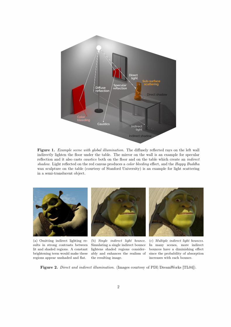
As illustrated in Figure 1, we can distinguish several ways in which light isreflected in a scene. A fundamental distinction is whether the light is reflectedonly once (direct light) or multiple times (indirect light) before it reaches theeye. Early lighting models in real-time graphics were limited to direct light,because it is fast to compute. Once it is determined whether a surface point isvisible from the light source, its lighting calculations are independent of otherobjects in the scene and can be fully described by local information such asmaterial, normal and light direction information. The main disadvantage ofthis approach is, however, that it produces a flat and unrealistic appearanceof the virtual scene (see Figure 2.a).
Lighting algorithms that additionally describe the light at a certain sur-face point as a function of other geometries in the scene are hence called globalillumination algorithms. Since light is naturally scattered many times beforereaching the eye, global illumination algorithms are necessary for synthesiz-ing naturally looking images of a virtual scene. Moreover, global lightingeffects are known to provide visual cues that help the viewer to understandthe volumetric structure and the spatial relationships of objects in the scene[Sto+04; AMHH08]. For these reasons, there is a high interest in developingreal-time global illumination techniques, most notably in the entertainment,architecture and design industry.
In this theses we will review the voxel cone tracing technique by develop-ing a renderer that demonstrates voxel cone tracing-based global illuminationeffects in real-time.
1
Direct shadow
Indirect shadow
Sub-surface scatteringSpecular
reflection
Colorbleeding
Caustics
Diffusereflection
Directlight
Indirectlight
Figure 1. Example scene with global illumination. The diffusely reflected rays on the left wallindirectly lighten the floor under the table. The mirror on the wall is an example for specularreflection and it also casts caustics both on the floor and on the table which create an indirectshadow. Light reflected on the red canvas produces a color bleeding effect, and the Happy Buddhawax sculpture on the table (courtesy of Stanford University) is an example for light scatteringin a semi-translucent object.
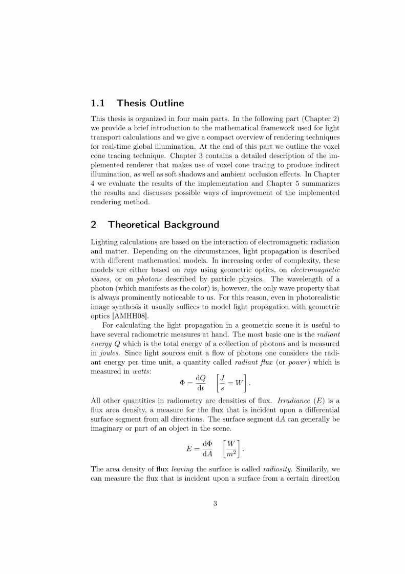
(a) Omitting indirect lighting re-sults in strong contrasts betweenlit and shaded regions. A constantbrightening term would make theseregions appear unshaded and flat.
(b) Single indirect light bounce.Simulating a single indirect bouncelightens shaded regions consider-ably and enhances the realism ofthe resulting image.
(c) Multiple indirect light bounces.In many scenes, more indirectbounces have a diminishing effectsince the probability of absorptionincreases with each bounce.
Figure 2. Direct and indirect illumination. (Images courtesy of PDI/DreamWorks [TL04]).
2
1.1 Thesis OutlineThis thesis is organized in four main parts. In the following part (Chapter 2)we provide a brief introduction to the mathematical framework used for lighttransport calculations and we give a compact overview of rendering techniquesfor real-time global illumination. At the end of this part we outline the voxelcone tracing technique. Chapter 3 contains a detailed description of the im-plemented renderer that makes use of voxel cone tracing to produce indirectillumination, as well as soft shadows and ambient occlusion effects. In Chapter4 we evaluate the results of the implementation and Chapter 5 summarizesthe results and discusses possible ways of improvement of the implementedrendering method.
2 Theoretical Background
Lighting calculations are based on the interaction of electromagnetic radiationand matter. Depending on the circumstances, light propagation is describedwith different mathematical models. In increasing order of complexity, thesemodels are either based on rays using geometric optics, on electromagneticwaves, or on photons described by particle physics. The wavelength of aphoton (which manifests as the color) is, however, the only wave property thatis always prominently noticeable to us. For this reason, even in photorealisticimage synthesis it usually suffices to model light propagation with geometricoptics [AMHH08].
For calculating the light propagation in a geometric scene it is useful tohave several radiometric measures at hand. The most basic one is the radiantenergy Q which is the total energy of a collection of photons and is measuredin joules. Since light sources emit a flow of photons one considers the radi-ant energy per time unit, a quantity called radiant flux (or power) which ismeasured in watts:
Φ =dQdt
[J
s= W
].
All other quantities in radiometry are densities of flux. Irradiance (E) is aflux area density, a measure for the flux that is incident upon a differentialsurface segment from all directions. The surface segment dA can generally beimaginary or part of an object in the scene.
E =dΦ
dA
[W
m2
].
The area density of flux leaving the surface is called radiosity. Similarily, wecan measure the flux that is incident upon a surface from a certain direction
3
dω. The direction is expressed as a solid angle and measured in steradians.The flux solid angle density is called radiant intensity :
I =dΦ
dω
[W
sr
].
Finally, we define radiance (L) as a measure for the flux at a differential surfacesegment dA coming from or leaving towards a certain direction dω. We definethis quantity as the radiant intensity per unit projected area normal to thebeam direction A⊥:
L =dIdA⊥
=d2Φ
dω dA⊥=
d2Φ
dω dA cos θ
[W
m2 sr
].
2.1 The Rendering EquationThe interactions of light under geometric optics approximation can be ex-pressed by the Rendering Equation [Kaj86] which defines the outgoing radi-ance Lo at a surface point x in direction ωo as the sum of emitted radianceLe and the reflected radiance Lr:
Lo(x,ωo) = Le(x,ωo) + Lr(x,ωo)
= Le(x,ωo) +
∫ωi∈Ω+
Li(x,ωi) fr(x,ωi → ωo) 〈N(x),ωi〉+ dωi . (2.1)
The reflected radiance is the weighted incident radiance Li coming from alldirections on the upper unit hemisphere Ω+ centered at the surface point xand oriented around the surface normal N(x). The vector ωi is the negativedirection of the incoming light, 〈· · ·〉+ is a dot product that is clamped to zero,and fr is the bidirectional reflectance distribution function or BRDF. The dotproduct is a weakening factor that accounts for the increasing incident arearelative to the projected area perpendicular to the ray as the incident angleincreases.
The BRDF describes the reflectance properties at a surface point x whenviewed from direction ωo. It is defined as the ratio of the radiance that isreflected toward ωo and the incoming radiance from direction ωi:
fr(x,ωi → ωo) =dLo(x,ωo)
dLi(x,ωi) cos θi dωi=
dLo(x,ωo)
dEi(x,ωi).
[1
sr
](2.2)
Physically based BRDFs must be both symmetric fr(ωi → ωo) = fr(ωo →ωi) and energy-conserving, i. e. that ∀ωo
∫Ω+ f(ωi → ωo)dωi ≤ 1. Two
4
dAφo
φi
θi
dωi
θo
dωo
n
x
(a)
T. Ritschel, C. Dachsbacher, T. Grosch, J. Kautz / The State of the Art in Interactive Global Illumination
To determine the incident radiance, Li, the ray casting oper-
),(o ωxL),( ii ωxL
),(e ωxL
x:
)(r xf
Figure 2: The rendering equation
ator is used to determine from which other surface locationthis radiance is emitted and reflected. It can be seen that therendering equation is a Fredholm integral equation of thesecond kind. The goal of global illumination algorithms isto compute Lo(x,w) for a given scene, materials and lightingLe.
Alternatively, the reflection integral can also be formulatedover the scenes’ surfaces S instead of directions. This impli-cates two modifications: first, a geometry term is introducedwhich accounts for the solid angle of a differential surface;second, the visibility function (sometimes considered part ofthe geometry term) determines the mutual visibility of twosurface points:
Lr(x,w) :=Z
SLi(s,wi) fr(x,wi ! w)hN(x),wii+ G(x,s)ds,
(3)
where S is the surface of the entire scene, w0 := s x thedifference vector from x to s, wi := w0/||w0|| the normalizeddifference vector and
G(x,s) :=hN(s),(wi)i+V (x,s)
||sx||2 ,
a distance term where V (x,s) is the visibility function that iszero if a ray between x and s is blocked and one otherwise.
Due to the repetitive application of the reflection integral,indirect lighting is distributed spatially and angularly and ulti-mately gets smoother with an increasing number of bounces.
Light In addition to geometry and material definition, theinitial lighting in a scene Le, obviously is an essential input tothe lighting simulation. In computer graphics several modelsof light sources, such as point, spot, directional, and arealights, exist.
Point lights are the simplest type of light sources, where theemission is specified as the position of the light source andthe directional distribution of spectral intensity. The incidentradiance due to a point light at a surface is then computedfrom these parameters.
Real-world light sources have a finite area that emits light,where the spatial, directional and spectral distribution can,in principle, be arbitrary. In computer graphics, often a di-rectional Lambertian emission is assumed, while a spatiallyvarying emission is often referred to as “textured area-light”.
Other commonly used models in computer graphics are: (1)spot lights, which can be considered as point lights with adirectionally focused emission; (2) directional lights, assum-ing parallel light rays; and (3) environment maps which storeincident radiance for every direction, however, assuming thatLi(x,wi) is independent of x, i. e., Li(x,wi) = Lenv(wi).
Reflectance The Bi-directional Reflectance DistributionFunction (BRDF) is a 4D function that defines how lightis reflected at a surface. The function returns the ratio of re-flected radiance exiting along wo to the irradiance incidenton the surface from direction wi. Physically plausible BRDFshave to be both symmetric fr(wi ! wo) = fr(wo ! wi) andenergy conserving
RW+ fr(wi ! wo)hN,wii+ dwi < 1. A spe-
cial case is the Lambertian BRDF which is independent ofthe outgoing direction, and the perfect mirror BRDF whichis a Dirac delta function in the direction of wi mirrored atthe surface normal at x. BRDFs inbetween these two extremaare often vaguely classified as directional-diffuse, glossy, andspecular. BRDFs can be spatially invariant, or vary acrossthe surface. In the latter case, BRDFs are called spatiallyvarying BRDFs or Bi-directional Texture Functions (BTFs).Many analytical BRDFs models, ranging from purely phe-nomenological to physically-based models, exist, which canbe either used as is, of fitted to measured BRDF or BTF data.If the material is not purely opaque, i. e., if light can enter orleave an object, then Bi-directional Scattering DistributionFunctions (BSDFs) are used which extend the domain fromthe hemisphere to the entire sphere.
Visibility Both versions of the rendering equation implysome form of visibility computation: Eq. 1 uses the ray cast-ing operator to determine the closest surface (for a givendirection) and Eq. 3 explicitly uses a binary visibility func-tion to test mutual visibility. Non-visible surfaces are usuallyreferred to as being occluded.
If the visibility is computed between a point and a surface,then the surface is said to be in shadow or be unshadowed.The visibility between a surface point and an area light sourceis non-binary resulting in soft shadows. A full survey of exist-ing (soft) shadow methods is beyond the scope of this reportand we refer to the survey of Hasenfratz et al. [HLHS03]and a recent book [ESAW11]. Note that many methods ded-icated to real-time rendering of soft-shadows often makesimplifying assumptions like planar rectangular light sources,isotropic emittance, Lambertian receivers, and so forth, thatallow for drastic speed-up compared to accurate computation(as in most GI methods), but also a loss of realism. Indirectlight bouncing off a surface is comparable to lighting froman area light source.
2.2. Volume rendering equation
Light transport in the presence of participating media is de-scribed by the volume rendering equation (Fig. 3). It com-
c 2011 The Author(s)Journal compilation c 2011 The Eurographics Association and Blackwell Publishing Ltd.
(b)
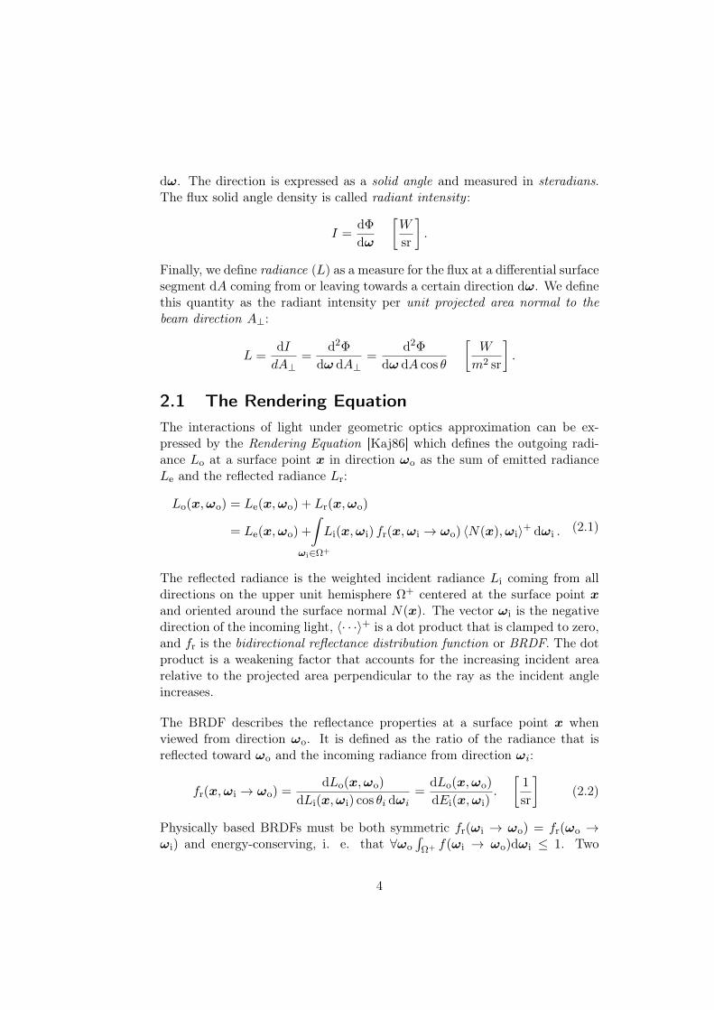
Figure 3. Visualization of the BRDF and the Rendering Equation. The BRDF(a) relates the incoming radiance from direction ωi with the outgoing radiance indirection ωo at a surface point x and thereby describes the scattering properties of asurface. θ and φ are the corresponding spherical coordinates of the solid angles. Theillustration of the Rendering Equation (b) is courtesy of [Rit+12].
extreme cases of the BRDF are the Lambertian BRDF which is constant forany pair (ωi, ωo), and the perfectly specular BRDF which is a Dirac deltafunction in the reflected viewing direction. Many surfaces can be modelled asa combination of these two extremes [Rit+12].
All of the functions defined above can additionally be parameterized bythe wavelength λ which allows modelling of colored materials and lights.
2.2 Rendering TechniquesThe Rendering Equation is very difficult to compute for several reasons. Onereason is that the hemisphere Ω+ describes a continuous space of solid angleswhich means that infinitely many directions and intersections with the scenegeometry must be regarded. Moreover, the integral in Equation 2.1 is definedin terms of itself (notice the Li on the right-hand side) which makes it a typeof integral equation to which no general algebraic solution is known [McG13].For these reasons, computations of the Rendering Equation generally involveapproximations.
There are several different approaches to approximating the RenderingEquation. In photo-realistic rendering the most important techniques includephoton mapping [Jen96], finite element methods such as the radiosity method[Gor+84] and Monte Carlo-based methods such as bidirectional path tracing[LW93]. These methods produce near-ideal results but are not directly suit-able for interactive applications. Instead, we make use of algorithms that arespecifically tailored for highly parallel computing on GPUs. A selection ofnotable real-time techniques are briefly summarized in the following list.
5
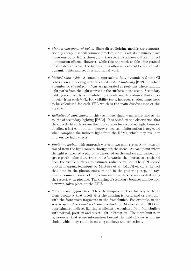
• Manual placement of lights. Since direct lighting models are computa-tionally cheap, it is still common practice that 3D artists manually placenumerous point lights throughout the scene to achieve diffuse indirectillumination effects. However, while this approach enables fine-grainedartistic decisions over the lighting, it is often impractical for scenes withdynamic lights and requires additional work.
• Virtual point lights. A common approach to fully dynamic real-time GIis based on a rendering method called Instant Radiosity [Kel97] in whicha number of virtual point light are generated at positions where randomlight paths from the light source hit the surfaces in the scene. Secondarylighting is efficiently accumulated by calculating the radiance that comesdirectly from each VPL. For visibility tests, however, shadow maps needto be calculated for each VPL which is the main disadvantage of thisapproach.
• Reflective shadow maps. In this technique, shadow maps are used as thesource of secondary lighting [DS05]. It is based on the observation thatthe directly lit surfaces are the only sources for secondary light bounces.To allow a fast computation, however, occlusion information is neglectedwhen sampling the indirect light from the RSMs, which may result inimplausible light effects.
• Photon mapping. This approach works in two main steps: First, rays aretraced from the light sources throughout the scene. At each point wherethe light is reflected a photon is deposited on the surface and cached in aspace-partitioning data structure. Afterwards, the photons are gatheredfrom the visible surfaces to estimate radiance values. The GPU-basedphoton mapping technique by McGuire et al. [ML09] exploits the factthat both in the photon emission and in the gathering step, all rayshave a common center of projection and can thus be accelerated usingthe rasterization pipeline. The tracing of secondary bounces and beyond,however, takes place on the CPU.
• Screen space approaches. These techniques work exclusively with thescene geometry that is left after the clipping is performed or even onlywith the front-most fragments in the framebuffer. For example, in thescreen space directional occlusion method by Ritschel et al. [RGS09],approximated indirect lighting is efficiently calculated from framebufferswith normal, position and direct light information. The main limitationis, however, that scene information beyond the field of view is not in-cluded which may result in missing shadows and reflections.
6
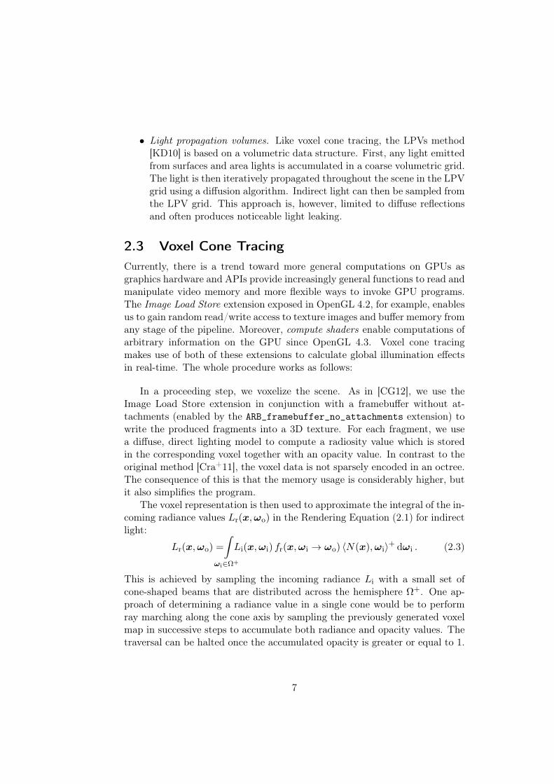
• Light propagation volumes. Like voxel cone tracing, the LPVs method[KD10] is based on a volumetric data structure. First, any light emittedfrom surfaces and area lights is accumulated in a coarse volumetric grid.The light is then iteratively propagated throughout the scene in the LPVgrid using a diffusion algorithm. Indirect light can then be sampled fromthe LPV grid. This approach is, however, limited to diffuse reflectionsand often produces noticeable light leaking.
2.3 Voxel Cone TracingCurrently, there is a trend toward more general computations on GPUs asgraphics hardware and APIs provide increasingly general functions to read andmanipulate video memory and more flexible ways to invoke GPU programs.The Image Load Store extension exposed in OpenGL 4.2, for example, enablesus to gain random read/write access to texture images and buffer memory fromany stage of the pipeline. Moreover, compute shaders enable computations ofarbitrary information on the GPU since OpenGL 4.3. Voxel cone tracingmakes use of both of these extensions to calculate global illumination effectsin real-time. The whole procedure works as follows:
In a proceeding step, we voxelize the scene. As in [CG12], we use theImage Load Store extension in conjunction with a framebuffer without at-tachments (enabled by the ARB_framebuffer_no_attachments extension) towrite the produced fragments into a 3D texture. For each fragment, we usea diffuse, direct lighting model to compute a radiosity value which is storedin the corresponding voxel together with an opacity value. In contrast to theoriginal method [Cra+11], the voxel data is not sparsely encoded in an octree.The consequence of this is that the memory usage is considerably higher, butit also simplifies the program.
The voxel representation is then used to approximate the integral of the in-coming radiance values Lr(x,ωo) in the Rendering Equation (2.1) for indirectlight:
Lr(x,ωo) =
∫ωi∈Ω+
Li(x,ωi) fr(x,ωi → ωo) 〈N(x),ωi〉+ dωi . (2.3)
This is achieved by sampling the incoming radiance Li with a small set ofcone-shaped beams that are distributed across the hemisphere Ω+. One ap-proach of determining a radiance value in a single cone would be to performray marching along the cone axis by sampling the previously generated voxelmap in successive steps to accumulate both radiance and opacity values. Thetraversal can be halted once the accumulated opacity is greater or equal to 1.
7
This approach, however, would introduce aliasing, and the quantity of sub-samples required to eliminate the aliasing would be impractical for real-timepurposes.
At this point, one can draw an analogy to 2D texture minification, since inboth cases it is necessary to integrate large regions of a texture while keepingaliasing effects at a minimum. A commonly used technique for this problem isto precompute a multi-resolution pyramid of the original texture, a so calledmipmap [Wil83], by repeatedly downsampling the texture by a factor of two.This can be done, for example, by averaging 2×2 pixel blocks at a time in eachmip image and storing the result in the corresponding mip level above. Wecan then sample the pre-filtered texture at an appropriate mip level insteadof relying on a multitude of samples.
The same principle can be applied to 3D textures by regarding 2 × 2 ×2 blocks during the downsampling. The radiance value of a cone is thendetermined by stepping along the axis of the cone and sampling the pre-filteredvoxel data at a mip level with a voxel size that corresponds to the current conediameter. The radiance and opacity values are interpolated between adjacenttexels in the 3D texture and between two mip levels, which results in smoothtransitions.
Voxel cone tracing enables us to approximate arbitrary BRDFs fr (Equa-tion 2.3) by arranging multiple cones with different apertures and weights onthe hemisphere Ω+. A specular BRDF, for example, can be represented bya single narrow cone in the direction of the viewing vector reflected aboutthe normal, and a diffuse BRDF can be achieved with a set of uniformly dis-tributed wide cones (∼5–12 suffice). Especially when using wide cones, thisapproach allows very fast, approximated evaluation of the lighting integralbecause the sampling rate can be quickly decreased when stepping throughcoarser mip levels of the voxel representation. Regarding the solid angle weintegrate over, the runtime behavior is thus converse to that of ray tracing.Moreover, relying on a data structure with a fixed resolution also decouplesthe cone tracing from the geometric complexity of the scene.
In summary, voxel cone tracing allows us to calculate LDS|DE light pathsin real-time and LDDE with particularly high efficiency. Furthermore, byaccumulating only the opacity values of the voxels, the same technique can beemployed for soft shadows and ambient occlusion effects which is explained indetail in the next chapter.
8
3 Implementation
The voxel cone tracing renderer which was implemented in the course of thisthesis, is written in the C++11 programming language and uses the OpenGL4.4 graphics API as well as the OpenGL Shading Language (GLSL) in version420 (shader model 5.0). For the scene and material management we make useof the graphics framework CVK (provided by Arbeitsgruppe Müller) whichis based on the Open Asset Import Library (Assimp 3.1.1). We extend partsof the CVK framework to satisfy requirements, e.g. for special framebufferconfigurations and for recompilation of shader programs for debugging pur-poses. Furthermore, we make use of the AntTweakBar library (in version1.16) to provide a simple user interface with options for adjusting several pa-rameters at runtime. The GLFW library (version 3.0.4) is used for creatingthe OpenGL context and handling user input, and we leverage the OpenGLMathematics Library (GLM 0.9.5.4) for GLSL-compliant arithmetics and lin-ear algebra functions and classes.
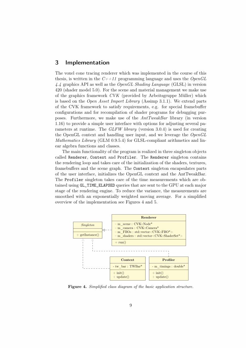
The main functionality of the program is realized in three singleton objectscalled Renderer, Context and Profiler. The Renderer singleton containsthe rendering loop and takes care of the initialization of the shaders, textures,framebuffers and the scene graph. The Context singleton encapsulates partsof the user interface, initializes the OpenGL context and the AntTweakBar.The Profiler singleton takes care of the time measurements which are ob-tained using GL_TIME_ELAPSED queries that are sent to the GPU at each majorstage of the rendering engine. To reduce the variance, the measurements aresmoothed with an exponentially weighted moving average. For a simplifiedoverview of the implementation see Figures 4 and 5.
Singleton
+ getInstance()
Renderer
– m_scene : CVK::Node*– m_camera : CVK::Camera*– m_FBOs : std::vector<CVK::FBO*>– m_shaders : std::vector<CVK::ShaderSet*>
+ run()
Context
- tw_bar : TWBar*
+ init()+ update()
Profiler
- m_timings : double*
+ init()+ update()
Figure 4. Simplified class diagram of the basic application structure.
9
Geometry buffer pass
Uncleared 3D textures Vertex data and texturesPosition map,Normal map
Clear and voxelization pass Shadow map pass Tangent map
Voxelized scenein lowest mip levels
Shadow map Depth map
Pre-integration pass Global illumination pass Direct illumination pass
3D textureswith complete mipmaps
Global illumination map,Ambient occlusion map
Direct illumination map
Compositing pass Diffuse color mapFinal image
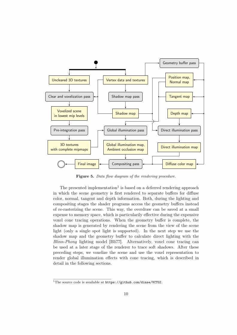
Figure 5. Data flow diagram of the rendering procedure.
The presented implementation1 is based on a deferred rendering approachin which the scene geometry is first rendered to separate buffers for diffusecolor, normal, tangent and depth information. Both, during the lighting andcompositing stages the shader programs access the geometry buffers insteadof re-rasterizing the scene. This way, the overdraw can be saved at a smallexpense to memory space, which is particularily effective during the expensivevoxel cone tracing operations. When the geometry buffer is complete, theshadow map is generated by rendering the scene from the view of the scenelight (only a single spot light is supported). In the next step we use theshadow map and the geometry buffer to calculate direct lighting with theBlinn-Phong lighting model [Bli77]. Alternatively, voxel cone tracing canbe used at a later stage of the renderer to trace soft shadows. After thesepreceding steps, we voxelize the scene and use the voxel representation torender global illumination effects with cone tracing, which is described indetail in the following sections.
1The source code is available at https://github.com/dinse/VCTGI.
10
(a) Conservative (b) 6-separating (c) Solid
Figure 2: Different kinds of voxelizations covered.
ing of multiple (identically-sized) voxels. A new triangle/box testthat fulfills these requirements is detailed in the following.
Given a triangleT with vertices v0, v1, v2 and an axis-aligned boxB(e.g. a voxel) with minimum corner p and maximum corner p+∆p,we observe that T overlaps B iff
a) T ’s plane overlaps B and
b) for each of the three coordinate planes (xy, xz, yz), the 2D pro-jections of T and B into this plane overlap.
To test for the plane overlap, similar to Haines and Wallace [1991],we determine T ’s normal n and the critical point
c =
(∆px, nx > 00, nx ≤ 0
,
∆py, ny > 00, ny ≤ 0
,
∆pz, nz > 00, nz ≤ 0
)T
and check whether p + c and the opposite box corner p + (∆p − c)are on different sides of the plane or one of them is on the plane,that is whether
(⟨n,p⟩ + d1
) (⟨n,p⟩ + d2
) ≤ 0, (1)
where d1 = ⟨n, c − v0⟩ and d2 = ⟨n, (∆p − c) − v0⟩.For the 2D projection overlap tests, we utilize edge functions[Pineda 1988], each evaluated at that corner of B’s projection, a 2Daxis-aligned box, that yields the largest value and hence is “most in-terior” with respect to the edge (cf. Fig. 3 a). More precisely, usingthe xy coordinate plane as example, we compute
nxyei= (−ei,y, ei,x)T ·
1, nz ≥ 0−1, nz < 0
dxyei= −⟨nxy
ei, vi,xy⟩ +max
0,∆pxn
xyei ,x
+max
0,∆pyn
xyei ,y
(2)
for all three edges ei = vi+1 mod 3 − vi and test whether
∧2
i=0
(⟨nxy
ei,pxy⟩ + d
xyei≥ 0)
(3)
holds true, indicating overlap. Because the evaluation points for theedge functions differ, it is additionally necessary to verify that T ’saxis-aligned bounding box actually overlaps B.
Consequently, for a given triangleT and box extent ∆p, T ’s bound-ing box, n, d1, d2, and n
xyei
, dxyei
, nxzei
, dxzei
, nyzei
, dyzei
(i = 0, 1, 2) can bedetermined in a setup stage. The actual overlap test for a box withminimum corner p then requires merely testing for bounding boxoverlap and checking the criteria in Eqs. 1 and 3.
v0
v1v2
ne0
ne1
ne2
+ +
+ v0
v1v2
ne0
ne1
ne2+ −
+
(a) Conservative (b) 6-separating
Figure 3: Critical points for evaluating the edge functions in the 2Dprojection overlap tests, annotated with the function result’s sign.
Comparison The current standard triangle/box overlap test byAkenine-Moller [2001] is based on the separating axis theorem(SAT). The tests for the coordinate axes (x, y, z) and the normal nare equivalent to our bounding box and plane overlap tests, respec-tively. Interestingly, the remaining 9 axes tested essentially corre-spond to our 2D edge normals n
xyei
, nxzei
, nyzei
(i = 0, 1, 2). However,while the SAT approach requires testing the projections of T and Bonto an axis for overlap, our method merely necessitates evaluatingan edge function and checking the result’s sign. As illustrated inFig. 4, the SAT test for one of these axes actually performs unnec-essary work. Of the two configurations where an axis is separating(a, c), i.e. the projections onto it don’t overlap, only the one wherethe box is in the exterior half-space of the corresponding edge (a)needs to be captured; the other one is already handled by the axisfor the more adjacent edge (c). Overall, the SAT-based triangle/boxoverlap test requires more instructions than our approach, and asetup-based formulation additionally involves more set-up quanti-ties in the per-box test part, hence consuming more registers whenimplemented on the GPU.
ne−
axis a
+ +−
(a) (b) (c)
Figure 4: Different configurations for SAT-based overlap test.
3.2 Triangle-parallel conservative voxelization
To obtain a conservative voxelization, all voxels overlapped byan input mesh’s triangles must be determined. One natural data-parallel approach to this computation is processing all trianglesin parallel, launching one thread per triangle. For each triangle,first the bounding box is determined and then all voxels inside thebounding box are tested for overlap utilizing our triangle/box over-lap test. If an overlap test passes, the corresponding voxel is set.
Note that we also consider voxels that are merely touched by thebounding box, which is important to make the voxelization inde-pendent of the tessellation of planar surfaces (cf. Fig. 5 a). More-over, since only voxels overlapped by the bounding box are pro-cessed in the first place, the bounding box overlap test can be omit-ted when running the triangle/box overlap test.
Voxel updates Each voxel’s state is encoded by a single bit in alinear array. With multiple triangles being processed concurrently,some of them may try to update the same 32-bit value at the sametime. We hence employ the atomic or function to avoid conflictingwrites and ultimately missing any update. Moreover, when loopingover the voxels within the bounding box, we make the inner-mostloop proceed in x direction, where adjacent voxels are stored inconsecutive bits. Instead of writing each set voxel instantaneously,we buffer the 32-bit value a voxel’s bit belongs to in a register andonly write it to memory once all relevant voxels within this 32-bitvalue have been processed, potentially saving many atomic updates.
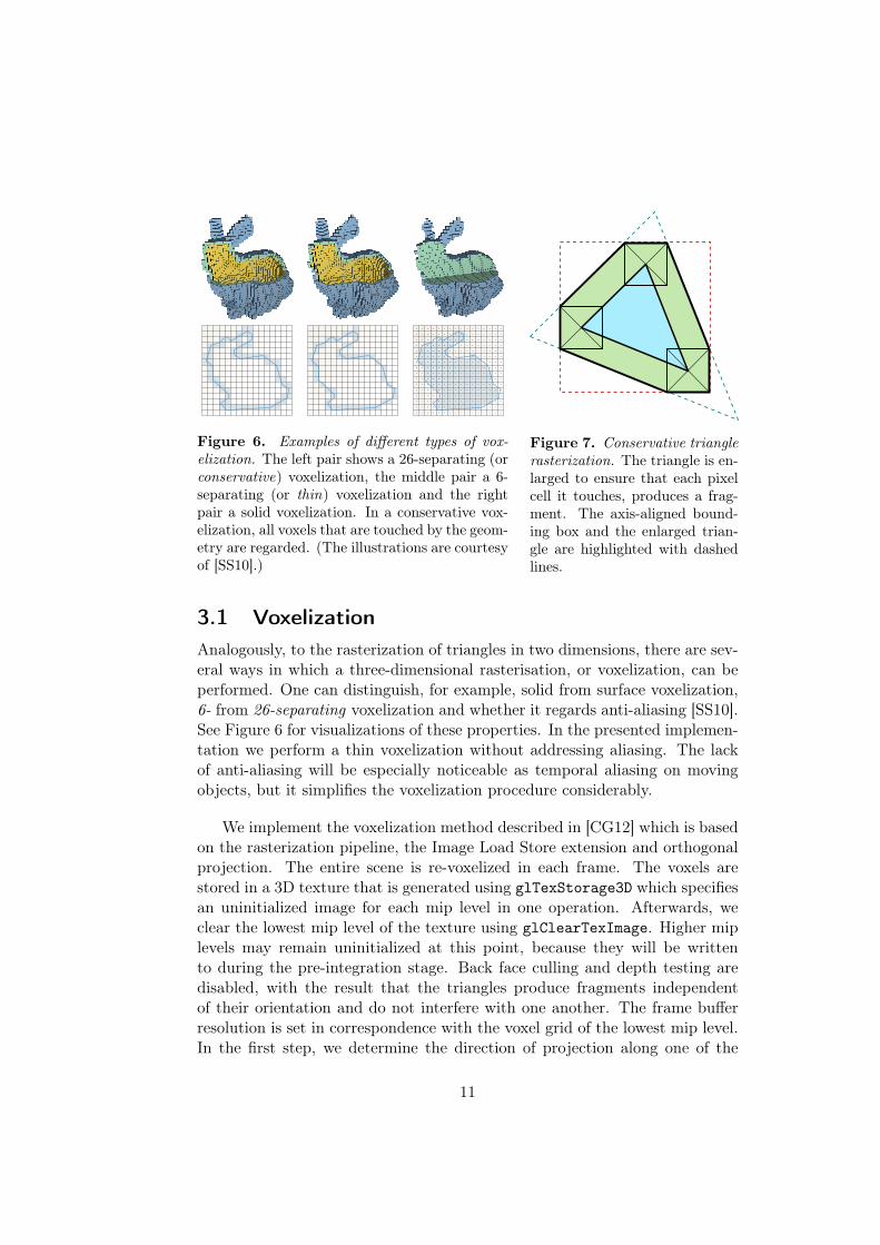
Figure 6. Examples of different types of vox-elization. The left pair shows a 26-separating (orconservative) voxelization, the middle pair a 6-separating (or thin) voxelization and the rightpair a solid voxelization. In a conservative vox-elization, all voxels that are touched by the geom-etry are regarded. (The illustrations are courtesyof [SS10].)
Figure 7. Conservative trianglerasterization. The triangle is en-larged to ensure that each pixelcell it touches, produces a frag-ment. The axis-aligned bound-ing box and the enlarged trian-gle are highlighted with dashedlines.
3.1 VoxelizationAnalogously, to the rasterization of triangles in two dimensions, there are sev-eral ways in which a three-dimensional rasterisation, or voxelization, can beperformed. One can distinguish, for example, solid from surface voxelization,6- from 26-separating voxelization and whether it regards anti-aliasing [SS10].See Figure 6 for visualizations of these properties. In the presented implemen-tation we perform a thin voxelization without addressing aliasing. The lackof anti-aliasing will be especially noticeable as temporal aliasing on movingobjects, but it simplifies the voxelization procedure considerably.
We implement the voxelization method described in [CG12] which is basedon the rasterization pipeline, the Image Load Store extension and orthogonalprojection. The entire scene is re-voxelized in each frame. The voxels arestored in a 3D texture that is generated using glTexStorage3D which specifiesan uninitialized image for each mip level in one operation. Afterwards, weclear the lowest mip level of the texture using glClearTexImage. Higher miplevels may remain uninitialized at this point, because they will be writtento during the pre-integration stage. Back face culling and depth testing aredisabled, with the result that the triangles produce fragments independentof their orientation and do not interfere with one another. The frame bufferresolution is set in correspondence with the voxel grid of the lowest mip level.In the first step, we determine the direction of projection along one of the
11
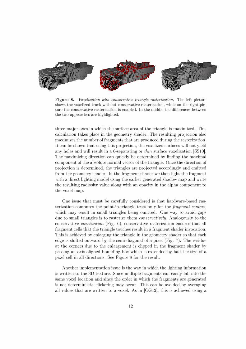
Figure 8. Voxelization with conservative triangle rasterization. The left pictureshows the voxelized truck without conservative rasterization, while on the right pic-ture the conservative rasterization is enabled. In the middle the differences betweenthe two approaches are highlighted.
three major axes in which the surface area of the triangle is maximized. Thiscalculation takes place in the geometry shader. The resulting projection alsomaximizes the number of fragments that are produced during the rasterization.It can be shown that using this projection, the voxelized surfaces will not yieldany holes and will result in a 6-separating or thin surface voxelization [SS10].The maximizing direction can quickly be determined by finding the maximalcomponent of the absolute normal vector of the triangle. Once the direction ofprojection is determined, the triangles are projected accordingly and emittedfrom the geometry shader. In the fragment shader we then light the fragmentwith a direct lighting model using the earlier generated shadow map and writethe resulting radiosity value along with an opacity in the alpha component tothe voxel map.
One issue that must be carefully considered is that hardware-based ras-terization computes the point-in-triangle tests only for the fragment centers,which may result in small triangles being omitted. One way to avoid gapsdue to small triangles is to rasterize them conservatively. Analogously to theconservative voxelization (Fig. 6), conservative rasterization ensures that allfragment cells that the triangle touches result in a fragment shader invocation.This is achieved by enlarging the triangle in the geometry shader so that eachedge is shifted outward by the semi-diagonal of a pixel (Fig. 7). The residueat the corners due to the enlargement is clipped in the fragment shader bypassing an axis-aligned bounding box which is extended by half the size of apixel cell in all directions. See Figure 8 for the result.
Another implementation issue is the way in which the lighting informationis written to the 3D texture. Since multiple fragments can easily fall into thesame voxel location and since the order in which the fragments are generatedis not deterministic, flickering may occur. This can be avoided by averagingall values that are written to a voxel. As in [CG12], this is achieved using a
12

simple moving average which is calculated as
An+1 =nAn +xi+1
n+ 1.
The fastest way to write to texture images from a shader is to use theimageStore operation. This is, however, not suitable for the averaging becausethe changes made with imageStore are not guaranteed to become visible forother threads during the rendering pass. Hence, we need to make use ofatomic image store operations which are also provided by the Image LoadStore extension. One limitation of this approach is that in OpenGL 4.4 atomicimage operations only support 32-bit integer values. For this reason, it isnecessary to bind the images in the R32UI format, in which the color and alphacomponents are represented by four concatenated unsigned 8-bit integers. Toavoid storing the number of samples n in a separate texture, we rely on a 4-bitinteger value which is encoded in the least significant bits of the voxel values.Minor disadvantages of this approach are that it reduces the color depth ofthe voxels by a factor of two and that at most 16 samples can be takeninto account, which may lead to flickering when voxelizing highly detailedgeometry.
Since the cone tracing pass depends on linear interpolation of the voxelvalues, it would be advantageous to leverage hardware-based interpolation forthis task. To circumvent color leaking from voxels with zero opacity duringlinear interpolation, it is necessary to store the color components of the voxelvalues pre-multiplied with the alpha component in the form (ra, ga, ba, a)T
[PD84].
3.2 Pre-IntegrationThe multi-resolution representation of the scene is generated using a computeshader. Compute shaders are an addition to the GLSL language since OpenGL4.3 and they allow us to use the GPU for computing arbitrary information.Compute shaders are invocated within a work group of many compute shaderinvocations which in turn is situated in a 3-dimensional space, called computespace. Each shader invocation can be identified with a 3D vector within thecompute space called gl_GlobalInvocationID. We use this ID to address thevoxel space.
Using a single texture for the mipmapping would result in a loss of lightdirection information. To reduce implausible lighting results, the mipmappedradiosity values are thus stored in six textures, one for each of the six directionsalong the coordinate axes. For illustrations of the light leaking problem seeFigures 11(b) and 12. The pre-integration is achieved by composing four voxels
13
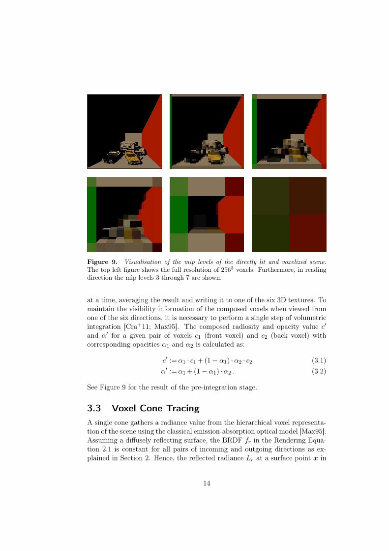
Figure 9. Visualisation of the mip levels of the directly lit and voxelized scene.The top left figure shows the full resolution of 2563 voxels. Furthermore, in readingdirection the mip levels 3 through 7 are shown.
at a time, averaging the result and writing it to one of the six 3D textures. Tomaintain the visibility information of the composed voxels when viewed fromone of the six directions, it is necessary to perform a single step of volumetricintegration [Cra+11; Max95]. The composed radiosity and opacity value c′
and α′ for a given pair of voxels c1 (front voxel) and c2 (back voxel) withcorresponding opacities α1 and α2 is calculated as:
c′ :=α1 · c1 + (1− α1) ·α2 · c2 (3.1)α′ :=α1 + (1− α1) ·α2 . (3.2)
See Figure 9 for the result of the pre-integration stage.
3.3 Voxel Cone TracingA single cone gathers a radiance value from the hierarchical voxel representa-tion of the scene using the classical emission-absorption optical model [Max95].Assuming a diffusely reflecting surface, the BRDF fr in the Rendering Equa-tion 2.1 is constant for all pairs of incoming and outgoing directions as ex-plained in Section 2. Hence, the reflected radiance Lr at a surface point x in
14
the Rendering Equation can be rewritten as
Lr(x,ωo) =
∫ωi∈Ω+
Li(x,ωi) fr(x,ωi → ωo) 〈N(x),ωi〉+ dωi
=ρ
π
∫ωi∈Ω+
Li(x,ωi) 〈N(x),ωi〉+ dωi,
where ρ is called albedo and describes the reflectivity of the surface. Next,we partition the integral into n cones and it is assumed that in each cone theincoming radiance is constant, which allows us to factor out Li:
Lr(x,ωo) =ρ
π
n∑k=1
∫ωi∈Ω+
k
Li(x,ωi) 〈N(x),ωi〉+ dωiLi const. for k⇔
Lr(x,ωo) =ρ
π
n∑k=1
Lk(x,ωk)
∫ωi∈Ω+
k
〈N(x),ωi〉+ dωi
=ρ
π
n∑k=1
Lk(x,ωk)Wk.
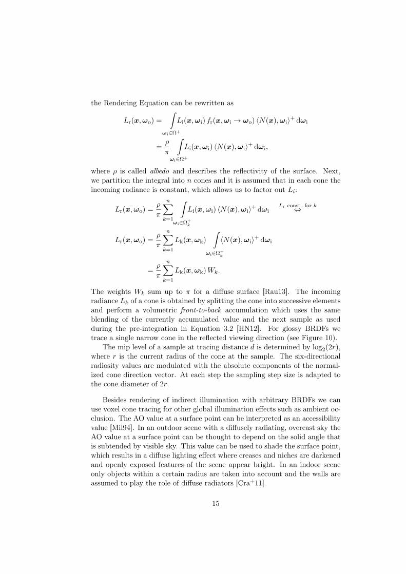
The weights Wk sum up to π for a diffuse surface [Rau13]. The incomingradiance Lk of a cone is obtained by splitting the cone into successive elementsand perform a volumetric front-to-back accumulation which uses the sameblending of the currently accumulated value and the next sample as usedduring the pre-integration in Equation 3.2 [HN12]. For glossy BRDFs wetrace a single narrow cone in the reflected viewing direction (see Figure 10).
The mip level of a sample at tracing distance d is determined by log2(2r),where r is the current radius of the cone at the sample. The six-directionalradiosity values are modulated with the absolute components of the normal-ized cone direction vector. At each step the sampling step size is adapted tothe cone diameter of 2r.
Besides rendering of indirect illumination with arbitrary BRDFs we canuse voxel cone tracing for other global illumination effects such as ambient oc-clusion. The AO value at a surface point can be interpreted as an accessibilityvalue [Mil94]. In an outdoor scene with a diffusely radiating, overcast sky theAO value at a surface point can be thought to depend on the solid angle thatis subtended by visible sky. This value can be used to shade the surface point,which results in a diffuse lighting effect where creases and niches are darkenedand openly exposed features of the scene appear bright. In an indoor sceneonly objects within a certain radius are taken into account and the walls areassumed to play the role of diffuse radiators [Cra+11].
15
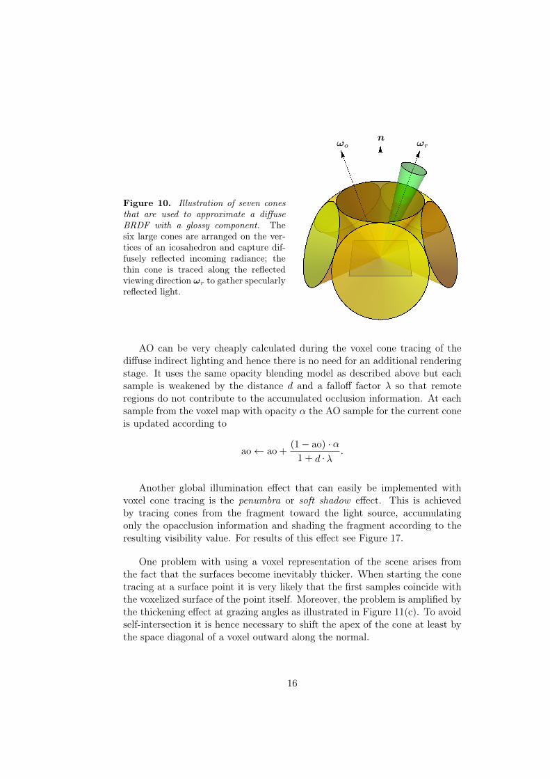
Figure 10. Illustration of seven conesthat are used to approximate a diffuseBRDF with a glossy component. Thesix large cones are arranged on the ver-tices of an icosahedron and capture dif-fusely reflected incoming radiance; thethin cone is traced along the reflectedviewing direction ωr to gather specularlyreflected light.
ωon
ωr
AO can be very cheaply calculated during the voxel cone tracing of thediffuse indirect lighting and hence there is no need for an additional renderingstage. It uses the same opacity blending model as described above but eachsample is weakened by the distance d and a falloff factor λ so that remoteregions do not contribute to the accumulated occlusion information. At eachsample from the voxel map with opacity α the AO sample for the current coneis updated according to
ao← ao +(1− ao) · α
1 + d ·λ.
Another global illumination effect that can easily be implemented withvoxel cone tracing is the penumbra or soft shadow effect. This is achievedby tracing cones from the fragment toward the light source, accumulatingonly the opacclusion information and shading the fragment according to theresulting visibility value. For results of this effect see Figure 17.
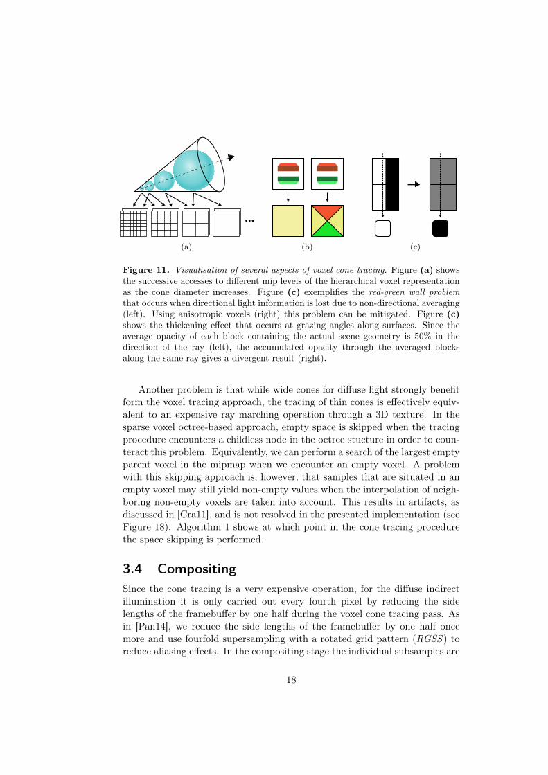
One problem with using a voxel representation of the scene arises fromthe fact that the surfaces become inevitably thicker. When starting the conetracing at a surface point it is very likely that the first samples coincide withthe voxelized surface of the point itself. Moreover, the problem is amplified bythe thickening effect at grazing angles as illustrated in Figure 11(c). To avoidself-intersection it is hence necessary to shift the apex of the cone at least bythe space diagonal of a voxel outward along the normal.
16
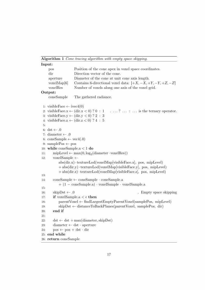
Algorithm 1 Cone tracing algorithm with empty space skipping.Input:
pos Position of the cone apex in voxel space coordinates.dir Direction vector of the cone.aperture Diameter of the cone at unit cone axis length.voxelMap[6] Contains 6-directional voxel data: [+X,−X,+Y,−Y,+Z,−Z]voxelRes Number of voxels along one axis of the voxel grid.
Output:coneSample The gathered radiance.
1: visibleFace← ivec4(0)2: visibleFace.x← (dir.x < 0) ? 0 : 1 . . . . ? . . . : . . . is the ternary operator.3: visibleFace.y← (dir.y < 0) ? 2 : 34: visibleFace.z ← (dir.z < 0) ? 4 : 55:6: dst← .07: diameter← .08: coneSample← vec4(.0)9: samplePos ← pos
10: while coneSample.a < 1 do11: mipLevel← max(0, log2(diameter · voxelRes))12: voxelSample ←
abs(dir.x) · textureLod(voxelMap[visibleFace.x], pos, mipLevel)+ abs(dir.y) · textureLod(voxelMap[visibleFace.y], pos, mipLevel)+ abs(dir.z) · textureLod(voxelMap[visibleFace.z], pos, mipLevel)
13:14: coneSample ← coneSample · coneSample.a
+ (1 − coneSample.a) · voxelSample · voxelSample.a15:16: skipDst ← .0 . Empty space skipping17: if voxelSample.a < ε then18: parentVoxel ← findLargestEmptyParentVoxel(samplePos, mipLevel)19: skipDst ← distanceToBackPlanes(parentVoxel, samplePos, dir)20: end if21:22: dst ← dst + max(diameter, skipDst)23: diameter ← dst · aperture24: pos ← pos + dst · dir25: end while26: return coneSample
17
…
(a) (b) (c)
Figure 11. Visualisation of several aspects of voxel cone tracing. Figure (a) showsthe successive accesses to different mip levels of the hierarchical voxel representationas the cone diameter increases. Figure (c) exemplifies the red-green wall problemthat occurs when directional light information is lost due to non-directional averaging(left). Using anisotropic voxels (right) this problem can be mitigated. Figure (c)shows the thickening effect that occurs at grazing angles along surfaces. Since theaverage opacity of each block containing the actual scene geometry is 50% in thedirection of the ray (left), the accumulated opacity through the averaged blocksalong the same ray gives a divergent result (right).
Another problem is that while wide cones for diffuse light strongly benefitform the voxel tracing approach, the tracing of thin cones is effectively equiv-alent to an expensive ray marching operation through a 3D texture. In thesparse voxel octree-based approach, empty space is skipped when the tracingprocedure encounters a childless node in the octree stucture in order to coun-teract this problem. Equivalently, we can perform a search of the largest emptyparent voxel in the mipmap when we encounter an empty voxel. A problemwith this skipping approach is, however, that samples that are situated in anempty voxel may still yield non-empty values when the interpolation of neigh-boring non-empty voxels are taken into account. This results in artifacts, asdiscussed in [Cra11], and is not resolved in the presented implementation (seeFigure 18). Algorithm 1 shows at which point in the cone tracing procedurethe space skipping is performed.
3.4 CompositingSince the cone tracing is a very expensive operation, for the diffuse indirectillumination it is only carried out every fourth pixel by reducing the sidelengths of the framebuffer by one half during the voxel cone tracing pass. Asin [Pan14], we reduce the side lengths of the framebuffer by one half oncemore and use fourfold supersampling with a rotated grid pattern (RGSS ) toreduce aliasing effects. In the compositing stage the individual subsamples are
18
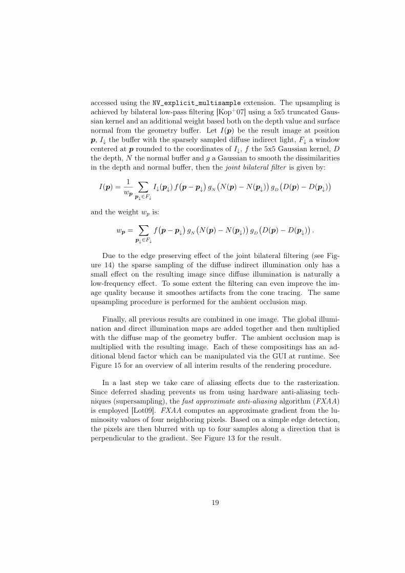
accessed using the NV_explicit_multisample extension. The upsampling isachieved by bilateral low-pass filtering [Kop+07] using a 5x5 truncated Gaus-sian kernel and an additional weight based both on the depth value and surfacenormal from the geometry buffer. Let I(p) be the result image at positionp, I↓ the buffer with the sparsely sampled diffuse indirect light, F↓ a windowcentered at p rounded to the coordinates of I↓, f the 5x5 Gaussian kernel, Dthe depth, N the normal buffer and g a Gaussian to smooth the dissimilaritiesin the depth and normal buffer, then the joint bilateral filter is given by:
I(p) =1
wp
∑p↓∈F↓
I↓(p↓) f(p− p↓
)gN(N(p)−N(p↓)
)gD(D(p)−D(p↓)
)and the weight wp is:
wp =∑
p↓∈F↓
f(p− p↓
)gN(N(p)−N(p↓)
)gD(D(p)−D(p↓)
).
Due to the edge preserving effect of the joint bilateral filtering (see Fig-ure 14) the sparse sampling of the diffuse indirect illumination only has asmall effect on the resulting image since diffuse illumination is naturally alow-frequency effect. To some extent the filtering can even improve the im-age quality because it smoothes artifacts from the cone tracing. The sameupsampling procedure is performed for the ambient occlusion map.
Finally, all previous results are combined in one image. The global illumi-nation and direct illumination maps are added together and then multipliedwith the diffuse map of the geometry buffer. The ambient occlusion map ismultiplied with the resulting image. Each of these compositings has an ad-ditional blend factor which can be manipulated via the GUI at runtime. SeeFigure 15 for an overview of all interim results of the rendering procedure.
In a last step we take care of aliasing effects due to the rasterization.Since deferred shading prevents us from using hardware anti-aliasing tech-niques (supersampling), the fast approximate anti-aliasing algorithm (FXAA)is employed [Lot09]. FXAA computes an approximate gradient from the lu-minosity values of four neighboring pixels. Based on a simple edge detection,the pixels are then blurred with up to four samples along a direction that isperpendicular to the gradient. See Figure 13 for the result.
19
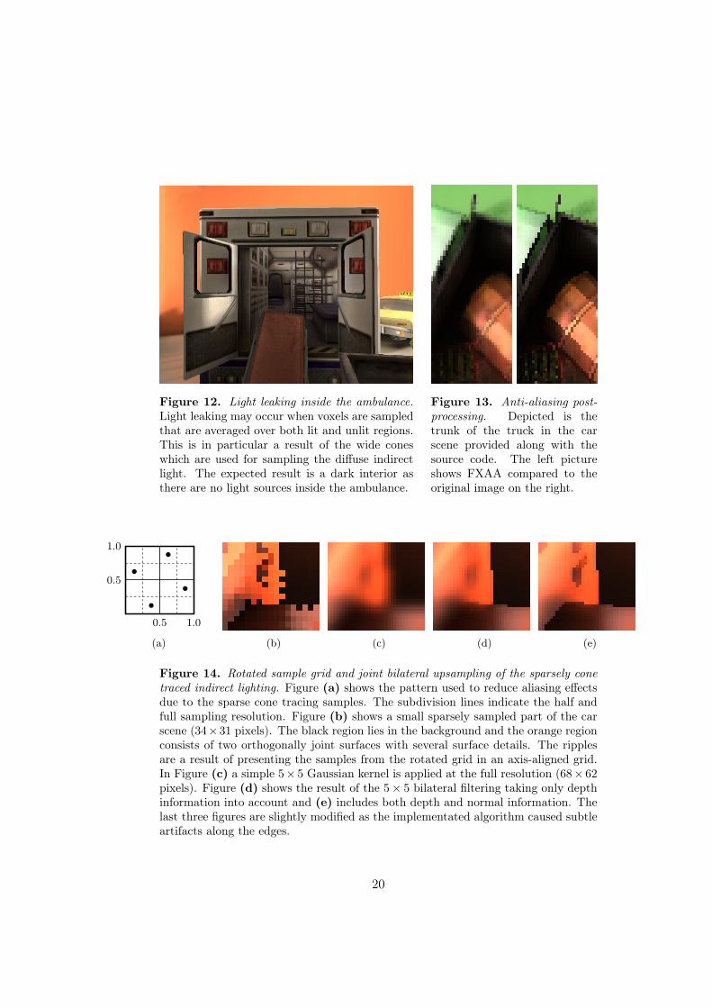
Figure 12. Light leaking inside the ambulance.Light leaking may occur when voxels are sampledthat are averaged over both lit and unlit regions.This is in particular a result of the wide coneswhich are used for sampling the diffuse indirectlight. The expected result is a dark interior asthere are no light sources inside the ambulance.
Figure 13. Anti-aliasing post-processing. Depicted is thetrunk of the truck in the carscene provided along with thesource code. The left pictureshows FXAA compared to theoriginal image on the right.
0.5
0.5
1.0
1.0
(a) (b) (c) (d) (e)
Figure 14. Rotated sample grid and joint bilateral upsampling of the sparsely conetraced indirect lighting. Figure (a) shows the pattern used to reduce aliasing effectsdue to the sparse cone tracing samples. The subdivision lines indicate the half andfull sampling resolution. Figure (b) shows a small sparsely sampled part of the carscene (34×31 pixels). The black region lies in the background and the orange regionconsists of two orthogonally joint surfaces with several surface details. The ripplesare a result of presenting the samples from the rotated grid in an axis-aligned grid.In Figure (c) a simple 5× 5 Gaussian kernel is applied at the full resolution (68× 62pixels). Figure (d) shows the result of the 5× 5 bilateral filtering taking only depthinformation into account and (e) includes both depth and normal information. Thelast three figures are slightly modified as the implementated algorithm caused subtleartifacts along the edges.
20

Figure 15. Overview of all rendering stages. The top row depicts the geometrybuffer, including the position, normal and diffuse color maps. In the second row twomip levels of the voxel representation, as well as the direct light map are shown. Inthe bottom row the indirect map (both diffuse and specular indirect lighting), theambient occlusion map and the final image are shown.
21
4 Results
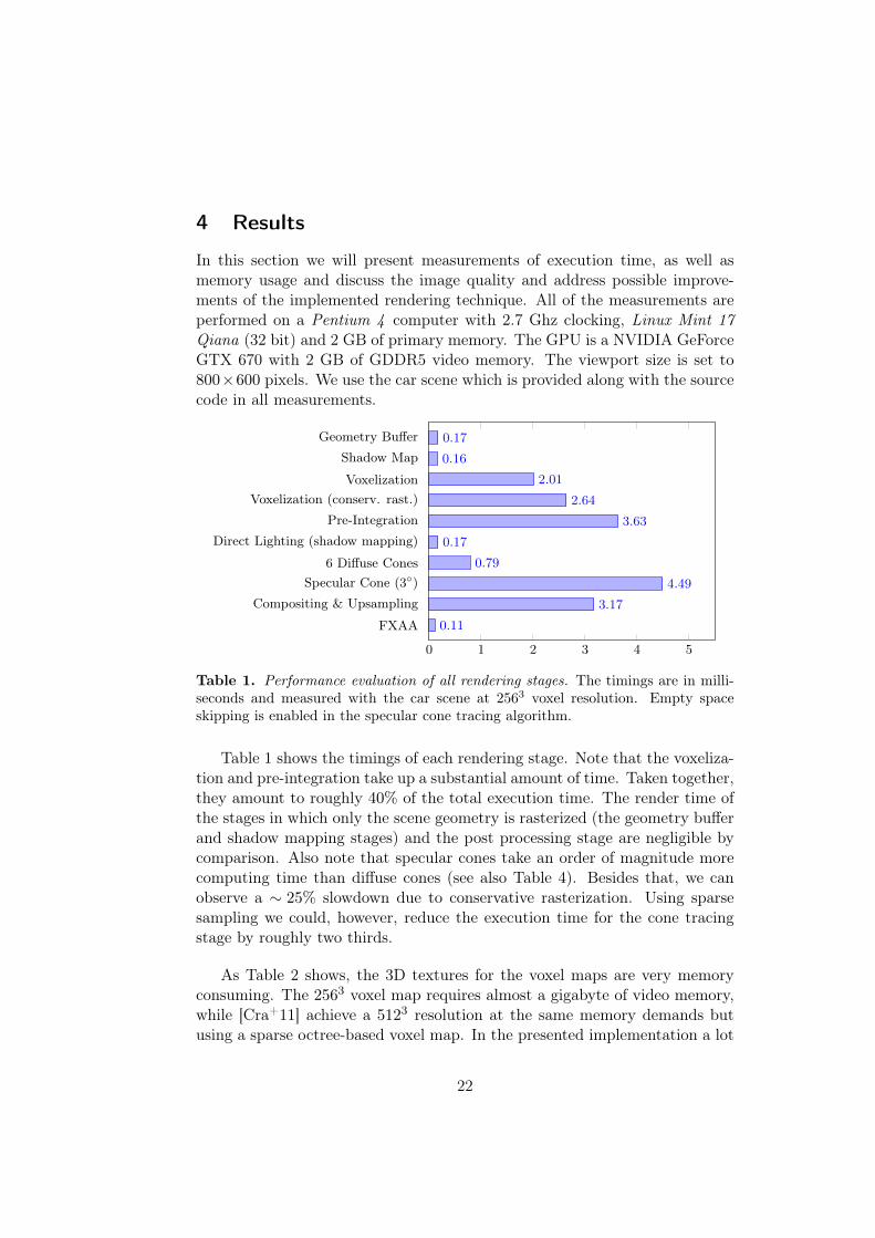
In this section we will present measurements of execution time, as well asmemory usage and discuss the image quality and address possible improve-ments of the implemented rendering technique. All of the measurements areperformed on a Pentium 4 computer with 2.7 Ghz clocking, Linux Mint 17Qiana (32 bit) and 2 GB of primary memory. The GPU is a NVIDIA GeForceGTX 670 with 2 GB of GDDR5 video memory. The viewport size is set to800×600 pixels. We use the car scene which is provided along with the sourcecode in all measurements.
0 1 2 3 4 5
Geometry Buffer
Shadow Map
VoxelizationVoxelization (conserv. rast.)
Pre-Integration
Direct Lighting (shadow mapping)
6 Diffuse ConesSpecular Cone (3)
Compositing & Upsampling
FXAA
0.17
0.16
2.01
2.64
3.63
0.17
0.79
4.49
3.17
0.11
Table 1. Performance evaluation of all rendering stages. The timings are in milli-seconds and measured with the car scene at 2563 voxel resolution. Empty spaceskipping is enabled in the specular cone tracing algorithm.
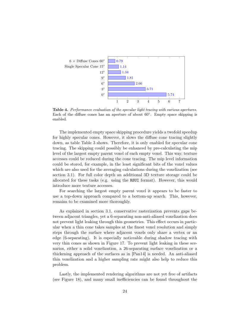
Table 1 shows the timings of each rendering stage. Note that the voxeliza-tion and pre-integration take up a substantial amount of time. Taken together,they amount to roughly 40% of the total execution time. The render time ofthe stages in which only the scene geometry is rasterized (the geometry bufferand shadow mapping stages) and the post processing stage are negligible bycomparison. Also note that specular cones take an order of magnitude morecomputing time than diffuse cones (see also Table 4). Besides that, we canobserve a ∼ 25% slowdown due to conservative rasterization. Using sparsesampling we could, however, reduce the execution time for the cone tracingstage by roughly two thirds.
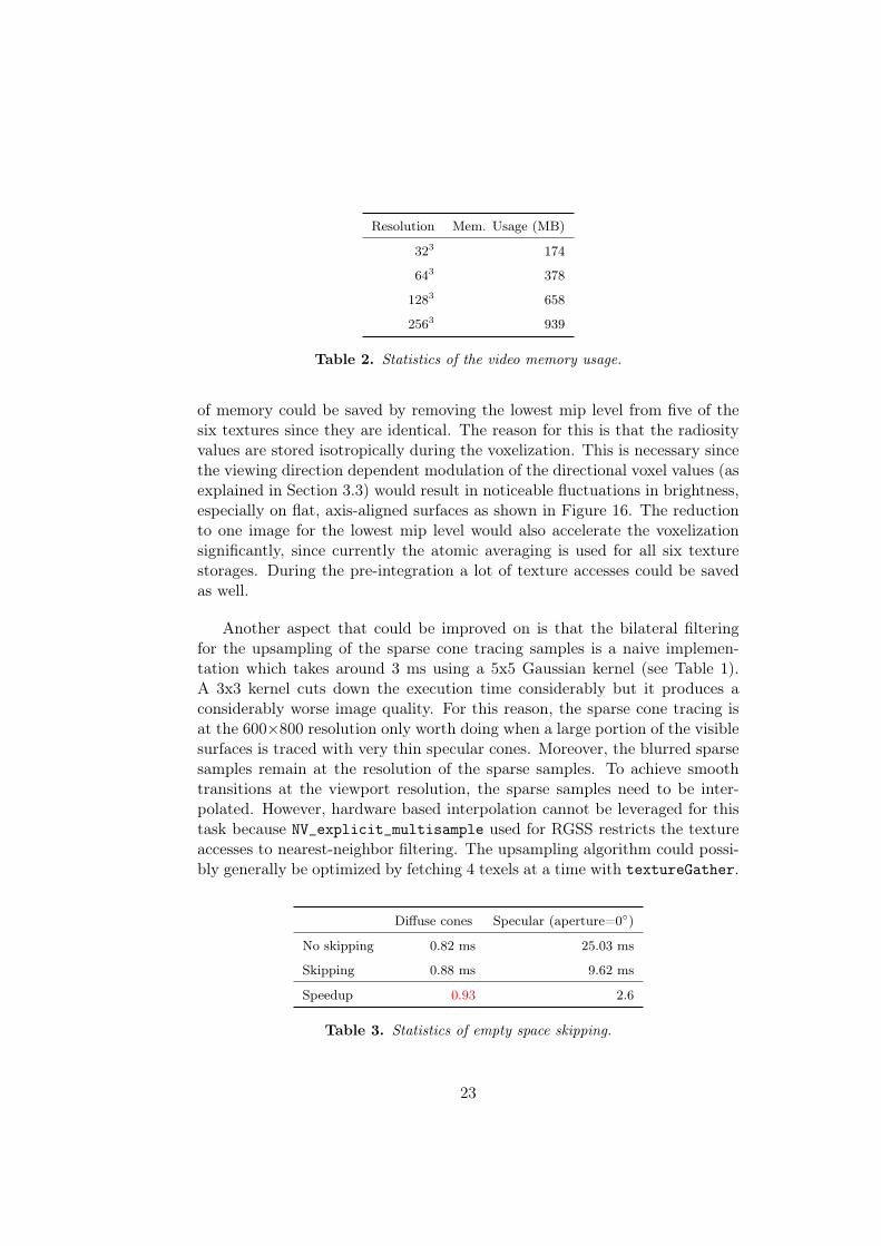
As Table 2 shows, the 3D textures for the voxel maps are very memoryconsuming. The 2563 voxel map requires almost a gigabyte of video memory,while [Cra+11] achieve a 5123 resolution at the same memory demands butusing a sparse octree-based voxel map. In the presented implementation a lot
22
Resolution Mem. Usage (MB)
323 174
643 378
1283 658
2563 939
Table 2. Statistics of the video memory usage.
of memory could be saved by removing the lowest mip level from five of thesix textures since they are identical. The reason for this is that the radiosityvalues are stored isotropically during the voxelization. This is necessary sincethe viewing direction dependent modulation of the directional voxel values (asexplained in Section 3.3) would result in noticeable fluctuations in brightness,especially on flat, axis-aligned surfaces as shown in Figure 16. The reductionto one image for the lowest mip level would also accelerate the voxelizationsignificantly, since currently the atomic averaging is used for all six texturestorages. During the pre-integration a lot of texture accesses could be savedas well.
Another aspect that could be improved on is that the bilateral filteringfor the upsampling of the sparse cone tracing samples is a naive implemen-tation which takes around 3 ms using a 5x5 Gaussian kernel (see Table 1).A 3x3 kernel cuts down the execution time considerably but it produces aconsiderably worse image quality. For this reason, the sparse cone tracing isat the 600×800 resolution only worth doing when a large portion of the visiblesurfaces is traced with very thin specular cones. Moreover, the blurred sparsesamples remain at the resolution of the sparse samples. To achieve smoothtransitions at the viewport resolution, the sparse samples need to be inter-polated. However, hardware based interpolation cannot be leveraged for thistask because NV_explicit_multisample used for RGSS restricts the textureaccesses to nearest-neighbor filtering. The upsampling algorithm could possi-bly generally be optimized by fetching 4 texels at a time with textureGather.
Diffuse cones Specular (aperture=0)
No skipping 0.82 ms 25.03 ms
Skipping 0.88 ms 9.62 ms
Speedup 0.93 2.6
Table 3. Statistics of empty space skipping.
23
1 2 3 4 5 6 7
6 × Diffuse Cones 60
Single Specular Cone 15
12
9
6
3
0
0.79
1.14
1.34
1.81
2.66
3.71
5.74
Table 4. Performance evaluation of the specular light tracing with various apertures.Each of the diffuse cones has an aperture of about 60. Empty space skipping isenabled.
The implemented empty space skipping procedure yields a twofold speedupfor highly specular cones. However, it slows the diffuse cone tracing slightlydown, as table Table 3 shows. Therefore, it is only enabled for specular conetracing. The skipping could possibly be enhanced by pre-calculating the miplevel of the largest empty parent voxel of each empty voxel. This way, textureaccesses could be reduced during the cone tracing. The mip level informationcould be stored, for example, in the least significant bits of the voxel valueswhich are also used for the averaging calculations during the voxelization (seesection 3.1). For full color depth an additional 3D texture storage could beallocated for these tasks (e.g. using the R8UI format). However, this wouldintroduce more texture accesses.
For searching the largest empty parent voxel it appears to be faster touse a top-down approach compared to a bottom-up search. This, however,remains to be examined more thoroughly.
As explained in section 3.1, conservative rasterization prevents gaps be-tween adjacent triangles, yet a 6-separating non-anti-aliased voxelization doesnot prevent light leaking through thin geometries. This effect occurs in partic-ular when a thin cone takes samples at the finest voxel resolution and simplysteps through the surface where adjacent voxels only share a vertex or anedge (6-separating). It is especially noticeable during shadow tracing withvery thin cones as shown in Figure 17. To prevent light leaking in these sce-narios, either a solid voxelization, a 26-separating surface voxelization or athickening approach of the surfaces as in [Pan14] is needed. An anti-aliasedthin voxelization and a higher sampling rate might also help to reduce thisproblem.
Lastly, the implemented rendering algorithms are not yet free of artifacts(see Figure 18), and many small inefficiencies can be found throughout the
24
5 10 15
Direct Lighting (shadow mapping)
Cone traced soft shadows 12
9
6
3
0
0.17
1.92
2.37
3.34
5.28
15.51
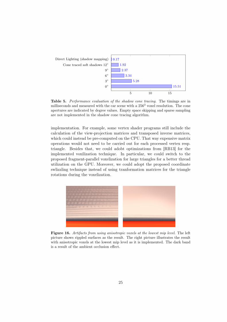
Table 5. Performance evaluation of the shadow cone tracing. The timings are inmilliseconds and measured with the car scene with a 2563 voxel resolution. The coneapertures are indicated by degree values. Empty space skipping and sparse samplingare not implemented in the shadow cone tracing algorithm.
implementation. For example, some vertex shader programs still include thecalculation of the view-projection matrices and transposed inverse matrices,which could instead be pre-computed on the CPU. That way expensive matrixoperations would not need to be carried out for each processed vertex resp.triangle. Besides that, we could adobt optimizations from [RB13] for theimplemented voxilization technique. In particular, we could switch to theproposed fragment-parallel voxelization for large triangles for a better threadutilization on the GPU. Moreover, we could adopt the proposed coordinateswlizzling technique instead of using tranformation matrices for the trianglerotations during the voxelization.
Figure 16. Artifacts from using anisotropic voxels at the lowest mip level. The leftpicture shows rippled surfaces as the result. The right picture illustrates the resultwith anisotropic voxels at the lowest mip level as it is implemented. The dark bandis a result of the ambient occlusion effect.
25
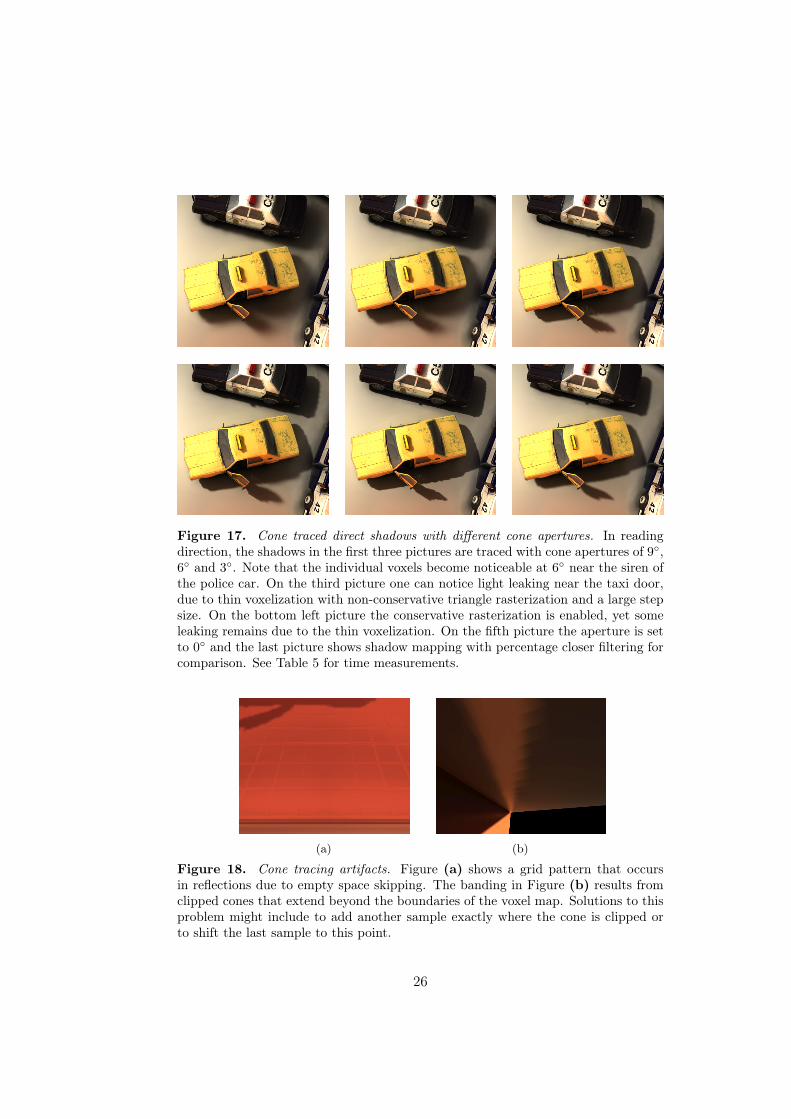
Figure 17. Cone traced direct shadows with different cone apertures. In readingdirection, the shadows in the first three pictures are traced with cone apertures of 9,6 and 3. Note that the individual voxels become noticeable at 6 near the siren ofthe police car. On the third picture one can notice light leaking near the taxi door,due to thin voxelization with non-conservative triangle rasterization and a large stepsize. On the bottom left picture the conservative rasterization is enabled, yet someleaking remains due to the thin voxelization. On the fifth picture the aperture is setto 0 and the last picture shows shadow mapping with percentage closer filtering forcomparison. See Table 5 for time measurements.
(a) (b)
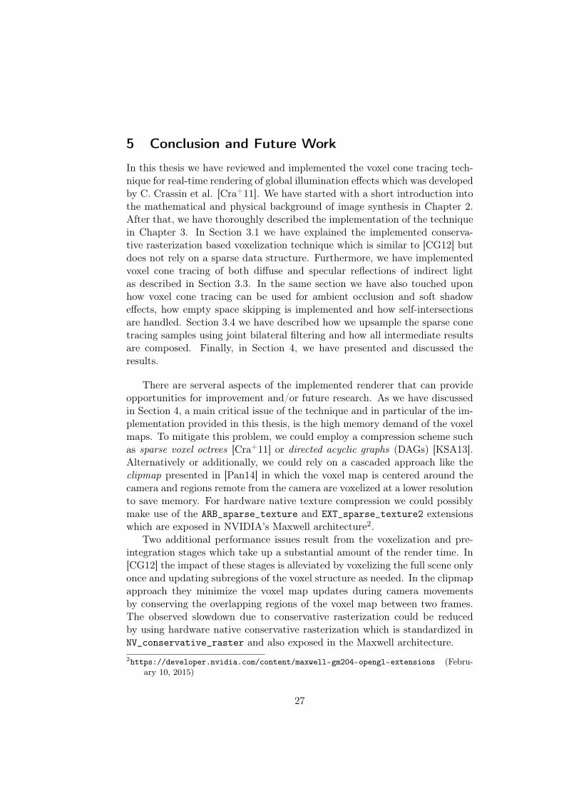
Figure 18. Cone tracing artifacts. Figure (a) shows a grid pattern that occursin reflections due to empty space skipping. The banding in Figure (b) results fromclipped cones that extend beyond the boundaries of the voxel map. Solutions to thisproblem might include to add another sample exactly where the cone is clipped orto shift the last sample to this point.
26
5 Conclusion and Future Work
In this thesis we have reviewed and implemented the voxel cone tracing tech-nique for real-time rendering of global illumination effects which was developedby C. Crassin et al. [Cra+11]. We have started with a short introduction intothe mathematical and physical background of image synthesis in Chapter 2.After that, we have thoroughly described the implementation of the techniquein Chapter 3. In Section 3.1 we have explained the implemented conserva-tive rasterization based voxelization technique which is similar to [CG12] butdoes not rely on a sparse data structure. Furthermore, we have implementedvoxel cone tracing of both diffuse and specular reflections of indirect lightas described in Section 3.3. In the same section we have also touched uponhow voxel cone tracing can be used for ambient occlusion and soft shadoweffects, how empty space skipping is implemented and how self-intersectionsare handled. Section 3.4 we have described how we upsample the sparse conetracing samples using joint bilateral filtering and how all intermediate resultsare composed. Finally, in Section 4, we have presented and discussed theresults.
There are serveral aspects of the implemented renderer that can provideopportunities for improvement and/or future research. As we have discussedin Section 4, a main critical issue of the technique and in particular of the im-plementation provided in this thesis, is the high memory demand of the voxelmaps. To mitigate this problem, we could employ a compression scheme suchas sparse voxel octrees [Cra+11] or directed acyclic graphs (DAGs) [KSA13].Alternatively or additionally, we could rely on a cascaded approach like theclipmap presented in [Pan14] in which the voxel map is centered around thecamera and regions remote from the camera are voxelized at a lower resolutionto save memory. For hardware native texture compression we could possiblymake use of the ARB_sparse_texture and EXT_sparse_texture2 extensionswhich are exposed in NVIDIA’s Maxwell architecture2.
Two additional performance issues result from the voxelization and pre-integration stages which take up a substantial amount of the render time. In[CG12] the impact of these stages is alleviated by voxelizing the full scene onlyonce and updating subregions of the voxel structure as needed. In the clipmapapproach they minimize the voxel map updates during camera movementsby conserving the overlapping regions of the voxel map between two frames.The observed slowdown due to conservative rasterization could be reducedby using hardware native conservative rasterization which is standardized inNV_conservative_raster and also exposed in the Maxwell architecture.2https://developer.nvidia.com/content/maxwell-gm204-opengl-extensions (Febru-
ary 10, 2015)
27
A fourth major issue is light leaking as a result of sampling large voxelswith coarsely approximated directional light information. A possible solutionmight be to use orthogonal basis functions (such as spherical harmonics) at thecoarse mip levels as proposed in [Rau13]. This could enable a more detaileddescription of the underlying scene geometry compared to the six-directionalapproach, while still allowing a fast evaluation of the regions of space thevoxels represent.
In conclusion, we have reviewed a state-of-the-art rendering technique thatconstitues an efficient alternative to other global illumination approaches. Itwill be interesting to see whether the high memory demands and the lightleaking can be further improved in future research.
28
References
[AMHH08] Tomas Akenine-Möller, Eric Haines, and Naty Hoffman. Real-Time Rendering, Third Edition. Taylor & Francis, 2008. isbn:9781439865293. url: http://www.realtimerendering.com/.
[Bli77] James F Blinn. “Models of light reflection for computer syn-thesized pictures”. In: ACM SIGGRAPH Computer Graphics.Vol. 11. 2. ACM. 1977, pp. 192–198.
[CG12] Cyril Crassin and Simon Green. “Octree-based sparse voxeliza-tion using the GPU hardware rasterizer”. In: OpenGL Insights(2012), pp. 303–318.
[Cra11] Cyril Crassin. “GigaVoxels: a voxel-based rendering pipeline forefficient exploration of large and detailed scenes”. PhD thesis.PhD thesis, Université de Grenoble, 2011.
[Cra+11] Cyril Crassin et al. “Interactive indirect illumination using voxelcone tracing”. In: Computer Graphics Forum. Vol. 30. 7. WileyOnline Library. 2011, pp. 1921–1930.
[DS05] Carsten Dachsbacher and Marc Stamminger. “Reflective shadowmaps”. In: Proceedings of the 2005 symposium on Interactive 3Dgraphics and games. ACM. 2005, pp. 203–231.
[Gor+84] Cindy M Goral et al. “Modeling the interaction of light be-tween diffuse surfaces”. In: ACM SIGGRAPH Computer Graph-ics. Vol. 18. 3. ACM. 1984, pp. 213–222.
[HN12] Eric Heitz and Fabrice Neyret. “Representing appearance andpre-filtering subpixel data in sparse voxel octrees”. In: Proceed-ings of the Fourth ACM SIGGRAPH/Eurographics conferenceon High-Performance Graphics. Eurographics Association. 2012,pp. 125–134.
[Jen96] Henrik W Jensen. “Global illumination using photon maps”. In:Rendering Techniques’ 96. Springer, 1996, pp. 21–30.
[Kaj86] James T Kajiya. “The rendering equation”. In: ACM SiggraphComputer Graphics. Vol. 20. 4. ACM. 1986, pp. 143–150.
[KD10] Anton Kaplanyan and Carsten Dachsbacher. “Cascaded light prop-agation volumes for real-time indirect illumination”. In: Proceed-ings of the 2010 ACM SIGGRAPH symposium on Interactive 3DGraphics and Games. ACM. 2010, pp. 99–107.
29
[Kel97] Alexander Keller. “Instant radiosity”. In: Proceedings of the 24thannual conference on Computer graphics and interactive tech-niques. ACM Press/Addison-Wesley Publishing Co. 1997, pp. 49–56.
[Kop+07] Johannes Kopf et al. “Joint Bilateral Upsampling”. In: ACMTransactions on Graphics (Proceedings of SIGGRAPH 2007).Vol. 26. 3. Association for Computing Machinery, Inc., 2007. url:http://research.microsoft.com/apps/pubs/default.aspx?id=78272.
[KSA13] Viktor Kämpe, Erik Sintorn, and Ulf Assarsson. “High Reso-lution Sparse Voxel DAGs”. In: ACM Transactions on Graph-ics 32.4 (July 7, 2013). url: highResolutionSparseVoxelDAGs.pdf.
[Lot09] T Lottes. FXAA (Whitepaper). Tech. rep. NVIDIA, 2009. url:http://developer.download.nvidia.com/assets/gamedev/files/sdk/11/FXAA_WhitePaper.pdf.
[LW93] Eric P Lafortune and Yves D Willems. “Bi-directional path trac-ing”. In: Proceedings of CompuGraphics. Vol. 93. 1993, pp. 145–153.
[Max95] Nelson Max. “Optical models for direct volume rendering”. In:Visualization and Computer Graphics, IEEE Transactions on 1.2(1995), pp. 99–108.
[McG13] Morgan McGuire. The Graphics Codex. v. 2.8. Apple Inc., 2013.
[Mil94] Gavin Miller. “Efficient algorithms for local and global acces-sibility shading”. In: Proceedings of the 21st annual conferenceon Computer graphics and interactive techniques. ACM. 1994,pp. 319–326.
[ML09] Morgan McGuire and David Luebke. “Hardware-accelerated globalillumination by image space photon mapping”. In: Proceedings ofthe Conference on High Performance Graphics 2009. ACM. 2009,pp. 77–89.
[Pan14] Alexey Panteleev. “Practical Real-Time Voxel-Based Global Illu-mination for Current GPUs”. Talk at the GPU Technology Con-ference 2014. 2014. url: http://on-demand-gtc.gputechconf.com/gtcnew/on-demand-gtc.php?searchByKeyword=SG4114.
[PD84] Thomas Porter and Tom Duff. “Compositing digital images”.In: ACM Siggraph Computer Graphics. Vol. 18. 3. ACM. 1984,pp. 253–259.
30
[Rau13] Randall Rauwendaal. “Voxel Based Indirect Illumination usingSpherical Harmonics”. PhD thesis. Oregon State University, Aug.2013. url: http://hdl.handle.net/1957/42266.
[RB13] Randall Rauwendaal and Mike Bailey. “Hybrid ComputationalVoxelization Using the Graphics Pipeline”. In: Journal of Com-puter Graphics Techniques (JCGT) 2.1 (2013), pp. 15–37. issn:2331-7418. url: http://jcgt.org/published/0002/01/02/.
[RGS09] Tobias Ritschel, Thorsten Grosch, and Hans-Peter Seidel. “Ap-proximating dynamic global illumination in image space”. In:Proceedings of the 2009 symposium on Interactive 3D graphicsand games. ACM. 2009, pp. 75–82.
[Rit+12] Tobias Ritschel et al. “The state of the art in interactive globalillumination”. In: Computer Graphics Forum. Vol. 31. 1. WileyOnline Library. 2012, pp. 160–188.
[SS10] Michael Schwarz and Hans-Peter Seidel. “Fast Parallel Surfaceand Solid Voxelization on GPUs”. In: ACM Transactions on Graph-ics 29.6 (Proceedings of SIGGRAPH Asia 2010) (Dec. 2010),179:1–179:9.
[Sto+04] William A Stokes et al. “Perceptual illumination components: anew approach to efficient, high quality global illumination ren-dering”. In: ACM Transactions on Graphics (TOG). Vol. 23. 3.ACM. 2004, pp. 742–749.
[TL04] Eric Tabellion and Arnauld Lamorlette. “An approximate globalillumination system for computer generated films”. In: ACM Trans-actions on Graphics (TOG). Vol. 23. 3. ACM. 2004, pp. 469–476.
[Wil83] LanceWilliams. “Pyramidal parametrics”. In: ACM Siggraph Com-puter Graphics. Vol. 17. 3. ACM. 1983, pp. 1–11.
Internet resources were last accessed on February 10, 2015.
31