vulnerability models - unitrentoeprints-phd.biblio.unitn.it/1282/1/nguyen-thesis.pdf ·...
TRANSCRIPT

PhD Dissertation
International Doctorate School in Information andCommunication Technologies
DISI ∼ University of Trento
EMPIRICAL METHODS FOR EVALUATING
VULNERABILITY MODELS
Viet Hung Nguyen
Advisor Committee
Professor Fabio Massacci Professor Massimiliano Di Penta
Università degli Studi di Trento Università degli Studi del Sannio
Professor Alexander Pretschner
Technische Universität München
Professor Laurie Williams
North Carolina State University
March 2014


ABSTRACT
THIS dissertation focuses on the following research question: “how to independently
and systematically validate empirical vulnerability models?”. Based on the survey on
past studies about the vulnerability discovery process, the dissertation has pointed
out several critical issues in the traditional methodology for evaluating the performance of
vulnerability discovery models (VDMs). Such issues did impact the conclusions of several
studies in the literature. To address such pitfalls, a novel empirical methodology and a data
collection infrastructure are proposed to conduct experiments that evaluate the empirical
performance of VDMs. The methodology consists of two quantitative analyses, namely qual-
ity and predictability analyses, which enable analysts to study the performance of VDMs, and
to compare them effectively.
The proposed methodology and the data collection infrastructure have been used to as-
sess several existing VDMs on many major versions of the major browsers (i.e., Chrome, Fire-
fox, Internet Explorer, and Safari). The extensive experimental analysis reveals an interesting
finding about the VDM performance in terms of quality and predictability: the simplest lin-
ear model is the most appropriate one for predicting vulnerability discovery trend within the
first twelve months since the release date of browser versions; later than that, logistic models
are more appropriate.
The analyzed vulnerability data exhibits the phenomenon of after-life vulnerabilities,
which have been discovered for the current version but also attributed to browser versions
out of support – dead versions. These vulnerabilities however may not actually exist, and
may have an impact on past scientific studies, or on compliance assessment. Therefore, this
dissertation has proposed a method to identify code evidence for vulnerabilities. The results
of the experiments show that a significant amount of vulnerabilities has been systematically
over-reported for old versions of browsers. Consequently, old versions of software seem to
have less vulnerabilities than reported.


ACKNOWLEDGEMENTS
I would like to express my deep appreciation to many people, without whom, I could not
finish the dissertation for my PhD graduation.
At first, I would like to thank Professor Fabio Massacci, who supervised my PhD work at
University of Trento. It is my luck to be his student and colleague. I would like to thank a lot
for his helpful advices, his endless patience, and his guidance during the last five years and
beyond. I have received invaluable supports from him for my travels to summer schools,
conferences, and project meetings. This helped to broaden not only my research horizonal,
but also my social knowledge.
I would like to thank Dr. Riccardo Scandariato who was the mentor for my internship at
University of Leuven. I have learnt many things from him. His working style has indeed in-
fluenced me a lot. I also want to thank all other colleagues at Ditri Net (University of Leuven)
for their kindness and helpfulness.
I am grateful to Professor Laurie William (North Carolina State University, United States),
Professor Alexander Pretschner (University of Munich, Germany), and Professor Massimil-
iano Di Penta (University of Sannio, Italy) for being committee members in my defence. They
have taken their time for reading my dissertation carefully, giving me many helpful and con-
structive feedback, and for challenging me with interesting questions that helped to improve
the quality of this dissertation.
I am thankful to Dr. Stephan Neuhaus for his collaboration in the very first year of my
PhD study. I also would like to thank to my colleagues and my friends at University of Trento.
However I decided not to list their names here because it is more likely that I would forget
some of them at the time of writing. They have contributed a lot of useful advices, discus-
sions, and also nice and welcome distraction.
I would like to thank to anonymous reviewers whom I will never know. Their comments
have frustrated me at the first sight, but they really were fruitful criticism that dramatically
helped me to improve my writing works, resulting in publications which the dissertation is
built upon.
Finally I would like to dedicate this dissertation to my sweetheart, Le Minh Sang Tran, for
her true love and deep understanding. Without her encouragements and supports I would
not be able to achieve that success. And to my family, who are always in my side uncondi-

tionally, even if they do not really understand what I am doing.
The dissertation has received financial support from University of Trento (Italy), and Eu-
ropean Union via FP7 R&D projects: SecureChange, NESSoS, and Seconomic.

CONTENTS
Abstract
Acknowledgements
Contents i
List of Tables v
List of Figures vii
Acronyms ix
1 Introduction 1
1.1 Contributions . . . . . . . . . . . . . . . . . . . . . . . . . . . . . . . . . . . . . . 2
1.2 Terminology . . . . . . . . . . . . . . . . . . . . . . . . . . . . . . . . . . . . . . . 3
1.3 Structure of the Dissertation . . . . . . . . . . . . . . . . . . . . . . . . . . . . . . 4
1.4 Publications . . . . . . . . . . . . . . . . . . . . . . . . . . . . . . . . . . . . . . . 7
2 Research Roadmap 9
2.1 Research Objective . . . . . . . . . . . . . . . . . . . . . . . . . . . . . . . . . . . 9
2.2 Research Method and Research Questions . . . . . . . . . . . . . . . . . . . . . . 10
2.2.1 Survey State-of-the-Art . . . . . . . . . . . . . . . . . . . . . . . . . . . . 12
2.2.2 Acquire Experimental Data . . . . . . . . . . . . . . . . . . . . . . . . . . 13
2.2.3 Perform Observation on Experimental Data . . . . . . . . . . . . . . . . 13
2.2.4 Invent Method(s) . . . . . . . . . . . . . . . . . . . . . . . . . . . . . . . . 14
2.2.5 Evaluate Method(s) . . . . . . . . . . . . . . . . . . . . . . . . . . . . . . . 15
2.3 Chapter Summary . . . . . . . . . . . . . . . . . . . . . . . . . . . . . . . . . . . . 16
3 A Survey of Empirical Vulnerability Studies 17
3.1 The Method to Conduct the Survey . . . . . . . . . . . . . . . . . . . . . . . . . . 18
3.2 A Qualitative Overview to Primary Studies . . . . . . . . . . . . . . . . . . . . . . 21
3.2.1 Fact Finding Studies . . . . . . . . . . . . . . . . . . . . . . . . . . . . . . 21
i

ii CONTENTS
3.2.2 Modeling Studies . . . . . . . . . . . . . . . . . . . . . . . . . . . . . . . . 24
3.2.3 Prediction Studies . . . . . . . . . . . . . . . . . . . . . . . . . . . . . . . 26
3.3 A Qualitative Analysis of Vulnerability Data Sources . . . . . . . . . . . . . . . . 28
3.3.1 Classification of Data Sources . . . . . . . . . . . . . . . . . . . . . . . . 28
3.3.2 Features in Data Sources . . . . . . . . . . . . . . . . . . . . . . . . . . . . 33
3.4 Chapter Summary . . . . . . . . . . . . . . . . . . . . . . . . . . . . . . . . . . . . 37
4 Data Infrastructure for Empirical Experiments 39
4.1 Software Infrastructure for Data Acquisition . . . . . . . . . . . . . . . . . . . . . 40
4.1.1 Acquiring Vulnerability Data for Firefox . . . . . . . . . . . . . . . . . . . 41
4.1.2 Acquiring Vulnerability Data for Chrome, IE, and Safari . . . . . . . . . 44
4.2 Potential Biases in Collected Data Sets . . . . . . . . . . . . . . . . . . . . . . . . 45
4.3 Market Share Data . . . . . . . . . . . . . . . . . . . . . . . . . . . . . . . . . . . . 47
4.4 Chapter Summary . . . . . . . . . . . . . . . . . . . . . . . . . . . . . . . . . . . . 49
5 After-Life Vulnerabilities 51
5.1 The Ecosystem of Software Evolution . . . . . . . . . . . . . . . . . . . . . . . . . 52
5.2 After-life Vulnerabilities and the Security Ecosystem . . . . . . . . . . . . . . . . 55
5.3 Threats to Validity . . . . . . . . . . . . . . . . . . . . . . . . . . . . . . . . . . . . 59
5.4 Chapter Summary . . . . . . . . . . . . . . . . . . . . . . . . . . . . . . . . . . . . 60
6 A Methodology to Evaluate VDMs 63
6.1 An Observation on the Traditional Validation Methodology . . . . . . . . . . . . 65
6.1.1 The Traditional Methodology . . . . . . . . . . . . . . . . . . . . . . . . . 66
6.1.2 The Validation Results of VDMs in Past Studies . . . . . . . . . . . . . . 67
6.2 Research Questions . . . . . . . . . . . . . . . . . . . . . . . . . . . . . . . . . . . 69
6.3 Methodology Overview . . . . . . . . . . . . . . . . . . . . . . . . . . . . . . . . . 72
6.4 Methodology Details . . . . . . . . . . . . . . . . . . . . . . . . . . . . . . . . . . 76
6.4.1 Step 1: Acquire the Vulnerability Data . . . . . . . . . . . . . . . . . . . . 76
6.4.2 Step 2: Fit a Vulnerability Discovery Model (VDM) to Observed Samples 78
6.4.3 Step 3: Perform Goodness-of-Fit Quality Analysis . . . . . . . . . . . . . 80
6.4.4 Step 4: Perform Predictability Analysis . . . . . . . . . . . . . . . . . . . 83
6.4.5 Step 5: Compare VDMs . . . . . . . . . . . . . . . . . . . . . . . . . . . . 85
6.5 Chapter Summary . . . . . . . . . . . . . . . . . . . . . . . . . . . . . . . . . . . . 86
7 The Evaluation of Existing VDMs 89

CONTENTS iii
7.1 Research Questions . . . . . . . . . . . . . . . . . . . . . . . . . . . . . . . . . . . 90
7.2 Experimental Setup . . . . . . . . . . . . . . . . . . . . . . . . . . . . . . . . . . . 90
7.2.1 The Software Infrastructure . . . . . . . . . . . . . . . . . . . . . . . . . . 91
7.2.2 Collected Vulnerability Data Sets . . . . . . . . . . . . . . . . . . . . . . . 92
7.3 An Assessment on Existing VDMs . . . . . . . . . . . . . . . . . . . . . . . . . . . 93
7.3.1 Goodness-of-Fit Analysis for VDMs . . . . . . . . . . . . . . . . . . . . . 94
7.3.2 Predictability Analysis for VDMs . . . . . . . . . . . . . . . . . . . . . . . 97
7.3.3 Comparison of VDMs . . . . . . . . . . . . . . . . . . . . . . . . . . . . . 99
7.4 Discussion . . . . . . . . . . . . . . . . . . . . . . . . . . . . . . . . . . . . . . . . 100
7.5 Threats to Validity . . . . . . . . . . . . . . . . . . . . . . . . . . . . . . . . . . . . 102
7.6 Chapter Summary . . . . . . . . . . . . . . . . . . . . . . . . . . . . . . . . . . . . 103
8 A Method to Assess Vulnerabilities Retro Persistence 105
8.1 Research Questions . . . . . . . . . . . . . . . . . . . . . . . . . . . . . . . . . . . 107
8.2 The Method to Identify Code Evidence for Vulnerability Claims . . . . . . . . . 108
8.2.1 Step 1: Acquire Vulnerability Data . . . . . . . . . . . . . . . . . . . . . . 110
8.2.2 Step 2: Locate Bug-Fix Commits . . . . . . . . . . . . . . . . . . . . . . . 111
8.2.3 Step 3: Identify Vulnerable Code Footprints . . . . . . . . . . . . . . . . 113
8.2.4 Step 4: Determine Vulnerability Evidences . . . . . . . . . . . . . . . . . 115
8.3 Related Work . . . . . . . . . . . . . . . . . . . . . . . . . . . . . . . . . . . . . . . 116
8.4 Chapter Summary . . . . . . . . . . . . . . . . . . . . . . . . . . . . . . . . . . . . 117
9 The Assessment of the NVD Vulnerability Claims 119
9.1 Research Questions . . . . . . . . . . . . . . . . . . . . . . . . . . . . . . . . . . . 120
9.2 The Assessing Experiment of Vulnerability Claims . . . . . . . . . . . . . . . . . 121
9.2.1 The Software Infrastructure . . . . . . . . . . . . . . . . . . . . . . . . . . 121
9.2.2 Descriptive Statistics . . . . . . . . . . . . . . . . . . . . . . . . . . . . . . 123
9.2.3 The Analysis on the Spurious Vulnerability Claims . . . . . . . . . . . . 127
9.3 The Impact of Spurious Vulnerability Claims . . . . . . . . . . . . . . . . . . . . 129
9.3.1 The Majority of Foundational Vulnerabilities . . . . . . . . . . . . . . . . 129
9.3.2 The Trend of Foundational Vulnerability Discovery . . . . . . . . . . . . 133
9.4 Threats to Validity . . . . . . . . . . . . . . . . . . . . . . . . . . . . . . . . . . . . 138
9.5 Chapter Summary . . . . . . . . . . . . . . . . . . . . . . . . . . . . . . . . . . . . 139
10 Conclusion 141
10.1 Summary of Contributions . . . . . . . . . . . . . . . . . . . . . . . . . . . . . . . 141

iv CONTENTS
10.2 Limitation and Future Directions . . . . . . . . . . . . . . . . . . . . . . . . . . . 145
10.2.1 The Need of Experiment Replication . . . . . . . . . . . . . . . . . . . . 145
10.2.2 The Need of a Maturity Model for Vulnerability Data . . . . . . . . . . . 145
Bibliography 147
A Appendix 159
A.1 Details of Laplace Test for Quarterly Trends of Foundational Vulnerabilities . . 159

LIST OF TABLES
2.1 Summary of research questions. . . . . . . . . . . . . . . . . . . . . . . . . . . . . . . 11
3.1 Details of primary studies. . . . . . . . . . . . . . . . . . . . . . . . . . . . . . . . . . 20
3.2 Classification of vulnerability data sources. . . . . . . . . . . . . . . . . . . . . . . . 30
3.3 Vulnerability data sources in past studies. . . . . . . . . . . . . . . . . . . . . . . . . 31
3.4 Potential features in a vulnerability data source. . . . . . . . . . . . . . . . . . . . . 34
3.5 Features of vulnerabilities data sources. . . . . . . . . . . . . . . . . . . . . . . . . . 35
4.1 Vulnerability data sources of browsers. . . . . . . . . . . . . . . . . . . . . . . . . . . 40
4.2 Descriptive statistics of browsers market share. . . . . . . . . . . . . . . . . . . . . . 49
5.1 Vulnerabilities in Firefox . . . . . . . . . . . . . . . . . . . . . . . . . . . . . . . . . . 58
5.2 Vulnerabilities in individual versions of Firefox . . . . . . . . . . . . . . . . . . . . . 58
6.1 Summary of VDM validation studies. . . . . . . . . . . . . . . . . . . . . . . . . . . . 67
6.2 Summary of VDM validation results (p-values) in the literature. . . . . . . . . . . . 68
6.3 Methodology overview. . . . . . . . . . . . . . . . . . . . . . . . . . . . . . . . . . . . 73
6.4 Formal definition of data sets. . . . . . . . . . . . . . . . . . . . . . . . . . . . . . . . 77
7.1 Descriptive statistics of observed data samples . . . . . . . . . . . . . . . . . . . . . 92
7.2 The VDMs in evaluation and their equation. . . . . . . . . . . . . . . . . . . . . . . . 93
7.3 The number of evaluated samples. . . . . . . . . . . . . . . . . . . . . . . . . . . . . 94
7.4 Suggested models for different usage scenarios. . . . . . . . . . . . . . . . . . . . . . 100
7.5 A potentially misleading results of overfitting VDMs in the largest horizon of browser
releases, using NVD data sets . . . . . . . . . . . . . . . . . . . . . . . . . . . . . . . . 101
7.6 Performance summary of VDMs. . . . . . . . . . . . . . . . . . . . . . . . . . . . . . 104
8.1 Overview of the proposed validation method. . . . . . . . . . . . . . . . . . . . . . . 109
8.2 The execution of the method on few Chrome vulnerabilities. . . . . . . . . . . . . . 115
9.1 Descriptive statistics for vulnerabilities of Chrome and Firefox . . . . . . . . . . . . 123
9.2 Descriptive statistics of vulnerability claims of Chrome. . . . . . . . . . . . . . . . . 124
9.3 Descriptive statistics of vulnerability claims of Firefox. . . . . . . . . . . . . . . . . . 125
v

vi List of Tables
9.4 The Wilcoxon signed-rank test results for the majority of foundational and inher-
ited vulnerabilities. . . . . . . . . . . . . . . . . . . . . . . . . . . . . . . . . . . . . . . 133
9.5 Number of events (i.e., significant quarterly trends) . . . . . . . . . . . . . . . . . . 135
A.1 Inconsistent events in Laplace test for quarterly trends in Chrome. . . . . . . . . . 171
A.2 Inconsistent events in Laplace test for quarterly trends in Firefox. . . . . . . . . . . 172

LIST OF FIGURES
2.1 Essential steps of the research methodology. . . . . . . . . . . . . . . . . . . . . . . 10
2.2 An overview to the research activities and produced artifacts. . . . . . . . . . . . . 12
3.1 Classification of primary studies yearly. . . . . . . . . . . . . . . . . . . . . . . . . . 19
3.2 The usage of data sources in all research topics (left) and its breakdown (right). . . 29
3.3 The usage of third-party data sources. . . . . . . . . . . . . . . . . . . . . . . . . . . 33
3.4 Usage of features by primary studies in each research topic. . . . . . . . . . . . . . 36
4.1 The infrastructure to collect vulnerability data for Firefox . . . . . . . . . . . . . . . 41
4.2 Different patterns of BUG and CVE references in MFSA. . . . . . . . . . . . . . . . . 43
4.3 The infrastructure to collect vulnerability data for Chrome, IE, and Safari. . . . . . 45
4.4 Histogram of number of MBugs per NVD entry, reported by MFSA. . . . . . . . . . 46
4.5 The market share of browsers since Jan 2008. . . . . . . . . . . . . . . . . . . . . . . 48
5.1 Release and retirement dates for Firefox. . . . . . . . . . . . . . . . . . . . . . . . . . 53
5.2 Size and lineage of Firefox source code . . . . . . . . . . . . . . . . . . . . . . . . . . 54
5.3 Firefox Users vs. LOC Users . . . . . . . . . . . . . . . . . . . . . . . . . . . . . . . . . 55
5.4 Vulnerabilities discovered in Firefox versions . . . . . . . . . . . . . . . . . . . . . . 56
6.1 Taxonomy of Vulnerability Discovery Models. . . . . . . . . . . . . . . . . . . . . . . 64
6.2 The two folds of the vulnerability counting issue. . . . . . . . . . . . . . . . . . . . . 71
6.3 Fitting the AML model to the NVD data sets for Firefox v3.0, v2.0, and v1.0. . . . . 79
6.4 Moving average of the temporal quality of sample AML and AT models. . . . . . . 83
6.5 The prediction qualities of AML and AT at fixed horizons τ = 12 and 24 to some
variable prediction time spans. . . . . . . . . . . . . . . . . . . . . . . . . . . . . . . 85
7.1 The software infrastructure of the experiment. . . . . . . . . . . . . . . . . . . . . . 91
7.2 The trend of temporal quality Qω=0.5(τ) of the VDMs in first 72 months. . . . . . . 95
7.3 The temporal quality distribution of each VDM in different periods of software
lifetime. . . . . . . . . . . . . . . . . . . . . . . . . . . . . . . . . . . . . . . . . . . . . 96
7.4 The predictability of VDMs in different prediction time spans (∆). . . . . . . . . . . 98
7.5 The comparison results among VDMs in some usage scenarios. . . . . . . . . . . . 99
vii

viii List of Figures
8.1 The vulnerable software and versions feature of the CVE-2008-7294. . . . . . . . . 106
8.2 Selected features from a CVE (a), and from an MFSA report (b). . . . . . . . . . . . 111
8.3 Bug-fix commits of Chrome (a) and Firefox (b). . . . . . . . . . . . . . . . . . . . . . 112
8.4 Excerpts of the output of diff (a), and of the output of annotate (b). . . . . . . . . 114
9.1 The software infrastructure for assessing the vulnerabilities retro persistence. . . . 122
9.2 The number of bugs per bug-fix commit in Chrome (a) and in Firefox (b). . . . . . 125
9.3 The complexity of bug-fix commits by number of source components (a) and by
number of vulnerable code footprints (b). . . . . . . . . . . . . . . . . . . . . . . . . 126
9.4 The average error rates (with error bars) of Chrome (a) and Firefox (b) along the
lifetime of individual versions. . . . . . . . . . . . . . . . . . . . . . . . . . . . . . . . 128
9.5 Foundational vulnerabilities by NVD: all vulnerability claims (left) and spurious
vulnerability claims excluded (right). . . . . . . . . . . . . . . . . . . . . . . . . . . . 131
9.6 The ratios of inherited vulnerabilities in Chrome and Firefox. . . . . . . . . . . . . 132
9.7 The actual discovery trends of foundational vulnerabilities. . . . . . . . . . . . . . . 135
9.8 The Laplace test for quarterly trends in Chrome v5 foundation vulnerabilities. . . 136
9.9 The Laplace test for quarterly trends in Firefox v3.0 foundation vulnerabilities. . . 136
9.10 The distribution of inconsistent events in National Vulnerability Database (NVD)
and Verified NVD. . . . . . . . . . . . . . . . . . . . . . . . . . . . . . . . . . . . . . . 137
A.1 Laplace test for trend in quarterly foundational vulnerability discovery for Chrome 160
A.2 Laplace test for trend in quarterly foundational vulnerability discovery for Firefox 166

ACRONYMS
AE Average Error
AB Average Bias
AIC Akaike Information Criteria
AKB Apple Knowledge Base
BSIMM Building Security In Maturity Model
CDG Component Dependency Graph
CERT Computer Emergency Response Team/Coordination Center
CIT Chrome Issue Tracker
CSV Comma Separated Values
CVE Common Vulnerabilities and Exposures
CVS Concurrent Version System
CVSS Common Vulnerabilities Scoring System
LoC Line of Code
MBug Mozilla Bugzilla
MDG Member Dependency Graph
MFSA Mozilla Foundation Security Advisories
MSB Microsoft Security Bulletin
NIST National Institute of Standards & Technology
NVD National Vulnerability Database
OSVDB Open Source Vulnerability Database
ix

x List of Figures
PCI DSS Payment Card Industry Data Security Standard
SCAP Security Content Automation Protocol
SDL Security Development Lifecycle
SQL Structured Query Language
SVM Support Vector Machine
VDM Vulnerability Discovery Model
CH
AP
TE
R
1INTRODUCTION
This chapter presents the motivation of this dissertation. It describes the overall
research questions and research method that drive the subsequent chapters. It also
summarizes the major contributions of this work, as well as published/in submission
publications on which the dissertation is built upon.
RECENT years have seen major efforts addressing the insecurity of software from guide-
lines for secure software development [McG09; HL03; HL06] to studies attempting to
understand the nature of vulnerabilities. Our survey of 59 recent studies in the field
from 2005 to 2012 whose contributions were (partially) relied on (or validated by) empirical
experiments shows fact finding papers (i.e., reporting the findings with/without some statis-
tics [Ozm05; OS06; Fre06; Res05; Li12; Sha12]), modeling papers (i.e., proposing mathemat-
ical models, or metrics, or methodologies concerning vulnerabilities [Alh07; And02; Res05;
You11; Joh08], or economic models [Shi12; AM13]), and prediction papers (i.e., predicting
the vulnerabilities in code base, [Shi11; CZ11; Geg09b; Neu07; Boz10]).
Vulnerability data sources now are employed not only in scientific studies, but also in
the compliance assessment for deployed software. The US National Institute of Standards
& Technology (NIST) Security Content Automation Protocol (SCAP) [Qui10], and Payment
Card Industry Data Security Standard (PCI DSS)[WC12] have been applied to evaluate the
compliance of software-related products. They both employ NVD. Any mistakes in NVD
might result in unfair fines raking hundreds of thousand of euros in companies. For instance,
if a product embeds an older version of browser (e.g., Chrome v4), it might lose compliance
1

2 CHAPTER 1. INTRODUCTION
with PCI DSS due to a large number of unfixed vulnerabilities. Then the product vendor
might either update to new version, or pay a fine, or be kicked out of the market.
This dissertation does not aim to provide a novel model of the vulnerability discovery
process, nor an outperform approach to early detect vulnerabilities. Instead, motivating by
the fact that several models on vulnerabilities are based on empirical experiments, the dis-
sertation lays its focus on the research question: “how to independently and systematically
validate empirical vulnerability models?".
The rest of this chapter is organized as follows. Section 1.1 briefly summarizes the main
contributions of the dissertation. Section 1.3 describes the chapters in the dissertation, as
well as a short summary for each chapter. Section 1.4 shows the ordinal publications that I
have (co)authored during the course of the PhD study.
1.1 Contributions
This section briefs the major contributions of the dissertation as follows.
i) An empirical methodology to evaluate the performance of time-based vulnerability dis-
covery models (VDMs). Several VDMs have been proposed e.g., [Alh05; Joh08; You11],
and have been claimed to be workable by their proponents. However, there were some
criticisms that these models might not work due to the violation of their implicit as-
sumptions [Ozm05]. We have pointed out some issues that might affect the valida-
tion experiments on the performance of VDMs. We have proposed a novel empiri-
cal methodology to validate the performance of VDMs. The methodology consists of
two quantitative analyses, namely quality and predictability, which enable analysts
to study the performance of VDMs, and to compare them effectively. Moreover, the
methodology addresses all identified issues that might be problematic while validat-
ing VDMs.
ii) A systematic assessment on the performance of existing VDMs based on our proposed
methodology. The conducted experiment assesses 8 out of 10 existing VDMs on 30
major versions of dominant web browsers (i.e., Chrome, Firefox, IE, and Safari). The
experiment results have revealed an interesting finding about the VDM performance
in terms of quality and predictability: the simplest linear model (Ω(t ) = Ax +B) is the
champion within first 12 months since the release date of browsers in predicting the
future trend of vulnerabilities; later then, logistic models are more appropriate.

1.2. TERMINOLOGY 3
iii) An empirical technique to quickly identify evidences for the existence of vulnerabilities
in retro versions of software. Apart from the findings about the majority of foundational
vulnerabilities [OS06] which are introduced in the very first version and continue to
survive in later versions, Chapter 5 shows that many of vulnerabilities have been re-
ported for “dead" software, which we called after-life vulnerabilities. Such vulnerabil-
ities are byproducts when researchers (or attackers) study and report security flaws in
the latest release of the software. These vulnerabilities however may not actually exist,
and may have an impact on past studies (e.g., Ozment and Schechter [OS06]), or on
compliance assessment (e.g., [Qui10; WC12]). Therefore, we have proposed a method
to quickly identify code evidence for vulnerabilities. The method has been empirically
tested in an experiment showing that a significant amount of vulnerabilities has been
systematically misreported for old versions of browsers. Consequently, old versions of
software (e.g., Chrome v4) seem to have less vulnerabilities than reported.
1.2 Terminology
Vulnerability is “an instance of a [human] mistake in the specification, development, or
configuration of software such that its execution can [implicitly or explicitly] violate
the security policy"[Krs98; Ozm07a].
Vulnerability entry is an entry, which reports security problem(s), in a vulnerability data
source, for instance NVD entries (a.k.a Common Vulnerabilities and Exposuress (CVEs))
of the NVD data source.
Vulnerability claim is a statement by a data source that a particular software version is vul-
nerable to a particular vulnerability entry. Figure 8.1 shows an example of the claims
of CVE-2008-7294.
Spurious vulnerability claim is a vulnerability claim which is not correct.
Data set is a collection of vulnerability data extracted from one or more data sources.
Release refers to a particular version of an application e.g., Firefox v1.0.
Horizon is a specific time interval sample. It is measured by the number of months since
the released date, e.g., 12 months since the release date.

4 CHAPTER 1. INTRODUCTION
Observed vulnerability sample (or observed sample, for short) is a time series of monthly
cumulative vulnerabilities of a major release since the first month after release to a
particular horizon.
Evaluated sample is a tuple of an observed sample, a VDM model, and the goodness-of-fit
of this model to this sample.
Commit is a unit of changes in source code, managed by the code base repository.
Bug-fix commit is a commit that contains changes to fix a (security) bug.
Vulnerable code footprint is a piece of code which is changed (or removed) in order to fix
a security bug. The intuition to identify such vulnerable code footprints is to compare
the revision where a security bug is fixed (i.e., bug-fix commit) to its immediate parent
revision. Pieces of code that appear in the parent revision, but not in the bug-fixed
revision are considered vulnerable code footprints, see Section 8.2.3 for more details.
1.3 Structure of the Dissertation
Chapter 1: Introduction. This chapter presents the motivation and the contributions of the
dissertation. It also describes the organization of the dissertation.
Chapter 2: Research Roadmap. This chapter presents the research objective of the disser-
tation, as well as research questions refined from the objective. It also describes how
other chapters could help to attain the research objective.
Chapter 3: A Survey of Empirical Vulnerability Studies. This chapter presents a survey on
empirical vulnerability studies. It focuses on the usage of data sources, and the major
focuses of those studies.
Related publication(s): This chapter has been partially published in:
• Fabio Massacci and Viet Hung Nguyen. “Which is the Right Source for Vulnera-
bilities Studies? An Empirical Analysis on Mozilla Firefox”. In: Proceedings of the
International ACM Workshop on Security Measurement and Metrics (MetriSec’10).
2010
Chapter 4: Data Infrastructure for Empirical Experiments. This chapter presents the data
infrastructure that will be used in the experiments conducted within the dissertation.
1.3. STRUCTURE OF THE DISSERTATION 5
This chapter includes the software infrastructure, and some heuristic rules to collect
the data from public sources.
Related publication(s): This chapter has been partially published in/ or being submit-
ted to:
• Fabio Massacci and Viet Hung Nguyen. “Which is the Right Source for Vulnera-
bilities Studies? An Empirical Analysis on Mozilla Firefox”. In: Proceedings of the
International ACM Workshop on Security Measurement and Metrics (MetriSec’10).
2010
• Fabio Massacci, Stephan Neuhaus, and Viet Hung Nguyen. “After-Life Vulnera-
bilities: A Study on Firefox Evolution, its Vulnerabilities and Fixes”. In: Proceed-
ings of the 2011 Engineering Secure Software and Systems Conference (ESSoS’11).
2011
• Viet Hung Nguyen and Fabio Massacci. An Empirical Methodology to Validated
Vulnerability Discovery Models. Tech. rep. (under submission to IEEE Transac-
tions on Software Engineering). University of Trento, 2013
Chapter 5: After-Life Vulnerabilities. This chapter presents our findings based on the col-
lected vulnerability data. We find that there are a lot of vulnerabilities discovered after
the browsers are out-of-support. We also revisit the claim about the majority of foun-
dation vulnerabilities made in [OS06].
Related publication(s): This chapter has been published in:
• Fabio Massacci, Stephan Neuhaus, and Viet Hung Nguyen. “After-Life Vulnera-
bilities: A Study on Firefox Evolution, its Vulnerabilities and Fixes”. In: Proceed-
ings of the 2011 Engineering Secure Software and Systems Conference (ESSoS’11).
2011
Chapter 6: A Methodology to Evaluate VDMs. This chapter describes a methodology to em-
pirically evaluate the performance of vulnerability discovery models (VDMs). The
chapter reviews the traditional validation methodology in past studies, as well as criti-
cal issues that potentially bias the experiments in past studies. The proposed method
addresses all these issues in its data collection and analysis steps. All notions and
concepts in the methodology are exemplified by real data from the experiment on
browsers.

6 CHAPTER 1. INTRODUCTION
Related publication(s): This chapters has been partially published in/or being submit-
ted to:
• Viet Hung Nguyen and Fabio Massacci. “An Independent Validation of Vulnera-
bility Discovery Models”. In: Proceeding of the 7th ACM Symposium on Informa-
tion, Computer and Communications Security (ASIACCS’12). 2012
• Viet Hung Nguyen and Fabio Massacci. An Empirical Methodology to Validated
Vulnerability Discovery Models. Tech. rep. (under submission to IEEE Transac-
tions on Software Engineering). University of Trento, 2013
Chapter 7: The Evaluation of Existing VDMs. This chapter applies the methodology pro-
posed in the previous chapter to conduct a validation experiment to review the perfor-
mance of existing VDMs. The experiment assesses the performance of eight VDMs in
different usage scenarios based on the vulnerability data of 30 major releases of domi-
nant browsers (i.e., Chrome, Firefox, IE, and Safari).
Related publication(s): This chapters has been partially published in/or being submit-
ted to:
• Viet Hung Nguyen and Fabio Massacci. “An Idea of an Independent Validation of
Vulnerability Discovery Models”. In: Proceedings of the 2012 Engineering Secure
Software and Systems Conference (ESSoS’12). 2012
• Viet Hung Nguyen and Fabio Massacci. “An Independent Validation of Vulnera-
bility Discovery Models”. In: Proceeding of the 7th ACM Symposium on Informa-
tion, Computer and Communications Security (ASIACCS’12). 2012
• Viet Hung Nguyen and Fabio Massacci. An Empirical Methodology to Validated
Vulnerability Discovery Models. Tech. rep. (under submission to IEEE Transac-
tions on Software Engineering). University of Trento, 2013
Chapter 8: A Method to Assess Vulnerabilities Retro Persistence. This chapter describes an
empirical method that automatically assess the retro persistence of vulnerabilities.
The proposed method extends the work by Sliwerski et al. [Sli05] to identify evidences
for the existence of vulnerabilities in retro versions of software.
Related publication(s): This chapter has been partially published in/or being submit-
ted to:

1.4. PUBLICATIONS 7
• Viet Hung Nguyen and Fabio Massacci. “The (Un) Reliability of NVD Vulnerable
Versions Data: an Empirical Experiment on Google Chrome Vulnerabilities”. In:
Proceeding of the 8th ACM Symposium on Information, Computer and Communi-
cations Security (ASIACCS’13). 2013
• Viet Hung Nguyen and Fabio Massacci. An Empirical Assessment of Vulnerabili-
ties Retro Persistence. Tech. rep. (to be submitted to Empirical Software Engineer-
ing, journal, Springer). University of Trento, 2013
Chapter 9: The Assessment of the NVD Vulnerability Claims. This chapter applies the pro-
posed assessment method for vulnerabilities retro persistence to conduct an experi-
ment on 33 major versions of Chrome and Firefox. The purpose is to test the proposed
method, and to validate the rule “version X and all its previous versions are vulnerable"
adopted by NVD security team. The experiment results have shown that, on average,
more than 30% of vulnerability claims to each of these versions are erroneous. The
errors do not negligibly happen by chance, but are significant and systematic phe-
nomenon along the browser age, and individual version age. Furthermore, we have
shown that these errors could negatively impact the conclusions withdrawn from some
vulnerability analyses.
Related publication(s): This chapter has been partially published in/or being submit-
ted to:
• Viet Hung Nguyen and Fabio Massacci. “The (Un) Reliability of NVD Vulnerable
Versions Data: an Empirical Experiment on Google Chrome Vulnerabilities”. In:
Proceeding of the 8th ACM Symposium on Information, Computer and Communi-
cations Security (ASIACCS’13). 2013
• Viet Hung Nguyen and Fabio Massacci. An Empirical Assessment of Vulnerabili-
ties Retro Persistence. Tech. rep. (to be submitted to Empirical Software Engineer-
ing, journal, Springer). University of Trento, 2013
Chapter 10: Conclusion. This chapter summarizes the major contributions of the disserta-
tion and describes possible future directions based on the results.
1.4 Publications
During my work as a PhD candidate I have (co)authored the following publications:

8 CHAPTER 1. INTRODUCTION
• Fabio Massacci and Viet Hung Nguyen. “Which is the Right Source for Vulnerabilities
Studies? An Empirical Analysis on Mozilla Firefox”. In: Proceedings of the International
ACM Workshop on Security Measurement and Metrics (MetriSec’10). 2010
• Viet Hung Nguyen and Le Minh Sang Tran. “Predicting Vulnerable Software Compo-
nents using Dependency Graphs”. In: Proceedings of the International ACM Workshop
on Security Measurement and Metrics (MetriSec’10). 2010
• Fabio Massacci, Stephan Neuhaus, and Viet Hung Nguyen. “After-Life Vulnerabilities:
A Study on Firefox Evolution, its Vulnerabilities and Fixes”. In: Proceedings of the 2011
Engineering Secure Software and Systems Conference (ESSoS’11). 2011
• Viet Hung Nguyen and Fabio Massacci. “An idea of an independent validation of vul-
nerability discovery models”. In: Proceedings of the 2012 Engineering Secure Software
and Systems Conference (ESSoS’12). 2012, pp. 89–96
• Viet Hung Nguyen and Fabio Massacci. “An Independent Validation of Vulnerability
Discovery Models”. In: Proceeding of the 7th ACM Symposium on Information, Com-
puter and Communications Security (ASIACCS’12). 2012
• Viet Hung Nguyen and Fabio Massacci. “The (Un) Reliability of NVD Vulnerable Ver-
sions Data: an Empirical Experiment on Google Chrome Vulnerabilities”. In: Proceed-
ing of the 8th ACM Symposium on Information, Computer and Communications Secu-
rity (ASIACCS’13). 2013
• Viet Hung Nguyen and Fabio Massacci. An Empirical Methodology to Validated Vulner-
ability Discovery Models. Tech. rep. (under submission to IEEE Transactions on Soft-
ware Engineering). University of Trento, 2013
• Viet Hung Nguyen and Fabio Massacci. An Empirical Assessment of Vulnerabilities
Retro Persistence. Tech. rep. (to be submitted to Empirical Software Engineering, jour-
nal, Springer). University of Trento, 2013
• Riccardo Scandariato, Viet Hung Nguyen, Fabio Massacci, and Wouter Joosen. Eval-
uating Text Features as Predictors of Security Vulnerabilities. Tech. rep. Univeristy of
Trento, University of Leuven, 2013

CH
AP
TE
R
2RESEARCH ROADMAP
This chapter presents the global research objective of the dissertation, as well as sev-
eral research questions refined from this objective. The chapter discusses the research
method to attain the research objective, and also discusses how various artifact pre-
sented in other chapters could fit together to obtain the global objective.
THIS chapter presents the general research objective of the dissertation, and the method-
ology to achieve the objective. The chapter describes various research questions re-
fined from the general objective, and gives an overview how and where these ques-
tions are answered in the dissertation. The chapter is organized as follows. Section 2.1
presents the global research objective. Section 2.2 discusses the research methodology and
various research questions refined from the objective. Section 2.3 summarizes the chapter.
2.1 Research Objective
Recent years have seen a growing interest of studies in quantitative security assessment and
the use of empirical methods on software vulnerabilities. Most of studies address the knowl-
edge problems such as what are the interesting phenomena in vulnerabilities?" or focus on
the ability to capture characteristics of vulnerabilities: e.g., what is the mathematical model
for the discovery of vulnerabilities? or could we predict vulnerabilities? Obviously, attaining
such insights would help to improve the security of software.
9

10 CHAPTER 2. RESEARCH ROADMAP
This dissertation is inspired by two key observations on past studies. First, only few stud-
ies [Res05; OS06] provided some claims about the quality of the data sources they used in
their experiments. Second, many proposed empirical models about vulnerabilities were
evaluated by researchers who are the authors of the models, except few independent dis-
cussion [OZMEN-07-QOP]. This motivates for the research objective that drives the rest of
this dissertation:
“How to perform an independent empirical evaluation of vulnerability models?”
2.2 Research Method and Research Questions
Figure 2.1 illustrates the steps of the research method used in this dissertation:
• Experimental setup. We gather background knowledge, facts, and requisites that need
to carry out the research.
• Observation. We observe on collected information in the previous step for interesting
phenomena.
• Induction. Based on observed phenomena plus background knowledge, we propose
a technique, a method, or an artifact that explains in more general terms the obser-
vations. Since our research goal focuses on an independent empirical evaluation of
vulnerability models, we have not invented our own version of a method or model
that predicted the observed data. Rather during the induction phase we have invented
methods to evaluate other work.
Experiment Setup
Observation
Induction
Evaluation
Figure 2.1: Essential steps of the research methodology.

2.2. RESEARCH METHOD AND RESEARCH QUESTIONS 11
Table 2.1: Summary of research questions.
Research Question Answered In
Activity: Survey State-of-the-Art
RQ1 Which are the popular data sources for vulnerability studies? Chapter 3
RQ2 Which data sources and features are used for which studies? Chapter 3
Activity: Invent Method(s)
RQ3 How to evaluate the performance of a VDM? Chapter 6
RQ4 How to compare between two or more VDMs? Chapter 6
RQ5 How to estimate the validity of a vulnerability claim to a retro version
of software?
Chapter 8
Activity: Evaluate Invented Method(s)
RQ6 Is the proposed VDM evaluation methodology effective in evaluating
VDMs?
Chapter 7
RQ7 Among existing VDMs, which one is the best? Chapter 7
RQ8 Is the proposed assessment method effective in assessing the retro
persistence of vulnerabilities?
Chapter 9
RQ9 To what extend are vulnerability claims by NVD trustworthy? Chapter 9
RQ10 To what extend does the bias in vulnerability claims by NVD (if any)
impact conclusions of a vulnerability analysis?
Chapter 9
• Evaluation. We conduct empirical experiments to evaluate the methods invented in
the previous step.
Figure 2.2 shows how we apply the research method in this dissertation, and how various
artifacts in subsequent chapters could fit to the research method. In this figure, rectangles
are activities and parallelograms represent artifacts produced in each activity. In general
the dissertation consists of following activities: Survey State-of-the-Art (Chapter 3), Acquire
Experimental Data (Chapter 4), Perform Observation on Experimental Data (Chapter 5, and
Chapter 6), Invent Method(s) (Chapter 6, Chapter 8), and Evaluate Invented Method(s) (Chap-
ter 7, Chapter 9).
As parts of these activities, we have conducted several empirical experiments. In these
experiments, we have refined the research objective into several technical research ques-
tions. Thus to achieve the final research objective, we are going to satisfy all these research

12 CHAPTER 2. RESEARCH ROADMAP
Survey State-of-the-Art
Acquire Experimental
Data
Perform Observation on
Experimental Data
Invent Method(s)
Evaluate Invented
Method(s)
Ex
pe
rim
en
t S
etu
pO
bs
erv
ati
on
Ind
uc
tio
nE
valu
ati
on
A Survey of Empirical
Vulnerability Studies
Infrastructure Data
Collection and Experiments
Observation on the Retro
Persistence of Vulnerability Claims
(After-Life and Foundational
Vulnerabilities)
Observation on
Vulnerability Discovery Models
Empirical Method to Evaluate
Vulnerability Discovery Models
Empirical Method to Evaluate the
Retro Persistence of Vulnerabilities
Assessment on Existing
Vulnerability Discovery Models
Assessment on Chrome and
Firefox vulnerabilities
Activity
Artifact
Legend
Figure 2.2: An overview to the research activities and produced artifacts.
questions, which will be described in the rest of this section, and are summarized in Ta-
ble 2.1.
The details of these activities and research questions are discussed in the sequel.
2.2.1 Survey State-of-the-Art
This activity is a part of the experiment setup where we gather background knowledge for
the research. Since the major focus of this dissertation lays on the area of empirical studies,
we conduct a survey about empirical studies on software vulnerabilities. The survey aims
to understand the following characteristics in past research studies: the research questions
which past studies have addressed, and the vulnerability data sources, particularly data fea-
tures, which past studies have used for their research topics. Formally, the survey addresses

2.2. RESEARCH METHOD AND RESEARCH QUESTIONS 13
the following research questions:
RQ1 Which are the popular data sources for vulnerability studies?
RQ2 Which data sources and features are used for which studies?
The outcome of this activity is a Survey of Empirical Vulnerability Studies. The details of the
survey is described in Chapter 3.
2.2.2 Acquire Experimental Data
Data is a common requisite for an empirical study about vulnerabilities since data plays a
crucial role in an empirical experiment. As a part of the experiment setup, this activity leads
to an Infrastructure Data Collection and Experiments to acquire vulnerability data. The in-
frastructure describes the software infrastructure and rules for compiling vulnerability data
from various data sources discussed in the survey of the previous activity. The details of the
data infrastructure are discussed in Chapter 4.
2.2.3 Perform Observation on Experimental Data
Based on the collected data, we can start the observation for interesting phenomena. We also
challenge the claims in past studies on the same data sources as we have an independent
validation of these claims. In particular, we have made the following observations:
• Observation on the Retro Persistence of Vulnerabilities (After-Life Vulnerabilities and
Foundational Vulnerabilities). We observe Firefox vulnerabilities in order to look for
an empirical evidence whether software-evolution-as-a-security-solution is actually a
solution. This observation reveals that a non-negligible amount of after-life vulnera-
bilities is a counter-evidence the solution. We also use the vulnerability data to check
the claim whether foundational vulnerabilities are the majority [OS06]. More detailed
discussion on this observation is described in Chapter 5.
On the other side, we observe an implicit rule in reporting vulnerability claims by the
NVD security team: they will claim all versions of a software vulnerable to a particu-
lar vulnerability without any additional validation if its description has something like
“version X and its previous versions are vulnerable”. This rule might be overdosed, and
could be a threat to validity of not only empirical vulnerability studies, but also assess-
ment of security compliance (e.g., SCAP, PCI DSS). This observation is presented in
Chapter 8.

14 CHAPTER 2. RESEARCH ROADMAP
• Observation on Vulnerability Discovery Models. We observe many issues that exist in
the traditional validation method to evaluate VDMs. They bias the outcome of VDM
validation experiments that follow this traditional method. Additionally, existing vali-
dation experiments in the past were conducted by the own authors of the model. This
observation motivated the invention of an empirical method that could independently
and systematically evaluate the performance of VDM. This observation is described in
Chapter 6.
2.2.4 Invent Method(s)
From the observations done in the previous step, we propose two empirical methods:
• Empirical Method to Evaluate Vulnerability Discovery Models. During the observation
activity, we have observed several issues in the traditional validation method for VDMs.
This potentially biases the outcome of VDM validation experiments that follow this
method. This motivates the following research questions:
RQ3 How to evaluate the performance of a VDM?
RQ4 How to compare between two or more VDMs?
We answer the above research questions by proposing an empirical method to eval-
uate the empirical performance of VDMs. The method consists of two key analyses:
goodness-of-fit quality analysis and goodness-of-fit predictability analysis. These anal-
yses allow researchers (or practitioners) to evaluate the performance of VDM, as well
as to compare VDMs. With these analyses, the proposed method delivers a better in-
sight than the traditional method. Moreover, the proposed method addresses all issues
of the traditional method. The outcome of a VDM validation experiment following the
proposed method is thus more reliable than the traditional analysis. We describe the
methodology in Chapter 6.
• Empirical Method to Evaluate the Retro Persistence of Vulnerabilities. The observation
on the retro persistence of vulnerability claims motivates following research question:
RQ5 How to estimate the validity of a vulnerability claim to a retro version of software?
We propose an empirical method that could quickly identify whether a vulnerability
claims made to a retro version of software is valid or not. The method quickly looks for
vulnerable code footprints, whose occurrences relate to the validity of vulnerabilities,

2.2. RESEARCH METHOD AND RESEARCH QUESTIONS 15
in the repository of the software. Then the method scans through the code base of
a software version, searching vulnerable code footprints. If none of them exists, it is
more likely that the vulnerability claim is not valid. The details of this method are
presented in Chapter 8.
2.2.5 Evaluate Method(s)
We conduct two experiments on browser vulnerabilities to test the two proposed empirical
methods. These experiments are:
• Assessment on Existing Vulnerability Discovery Models. We validate the methodology
to evaluate VDMs described in Chapter 6 by conducting an evaluation experiment on
several existing VDMs. The experiment addresses the following research questions:
RQ6 Is the proposed VDM evaluation methodology effective in evaluating VDMs?
RQ7 Among existing VDMs, which one is the best?
By the word “effective”, we mean the proposed methodology is able to evaluate VDMs
at least as good as the traditional methodology to conduct the experiment. We com-
pare the outcomes of each methodology. The comparison shows that the proposed
methodology provides more informative and interesting answers than the traditional
one. The experiment also studies the quality and predictability of VDMs in different
period of software lifetime. The details of this experiment are reported in Chapter 7.
• Assessment on Vulnerabilities of Chrome and Firefox. We test the method to assess the
validity of (retrospective) vulnerability claims in an experiment with many major ver-
sions of Chrome and Firefox. The experiment address the following research ques-
tions:
RQ8 Is the proposed assessment method effective in assessing the retro persistence of
vulnerabilities?
RQ9 To what extend are vulnerability claims by NVD trustworthy?
RQ10 To what extend does the bias in vulnerability claims by NVD (if any) impact con-
clusions of a vulnerability analysis?
Similarly, by the word "effective" we mean the proposed method is able to assess most
of vulnerability claims for the target applications (i.e., Chrome and Firefox). The out-
comes of the experiment present an empirical evidence that vulnerability claims by

16 CHAPTER 2. RESEARCH ROADMAP
NVD contains significant biases, which may significantly impact the conclusion of a
vulnerability analysis. The details of this experiment are presented in Chapter 9.
2.3 Chapter Summary
This chapter presented the research objective, as well as the research method to attain the
objective in this dissertation. The major focus of this work is to propose empirical method(s)
to evaluate empirical vulnerabilities. We followed the inductive inference research method-
ology to carry out the research. During the course of the dissertation, we have refined the
objective into several technical research questions. The answers to these research questions
will help to meet the research objective.
In the next section, we are going to describe the survey of empirical vulnerability studies.

CH
AP
TE
R
3A SURVEY OF EMPIRICAL VULNERABILITY
STUDIES
This chapter describes a survey about empirical vulnerability studies. The survey
focuses on the data usage of past studies, in which we study which data sources have
been used, and which data features are available in these data sources. We present
some descriptive statistics about the usage of data sources in these studies. Finally,
the survey briefly reviews past studies.
AN important stepping stone for conducting research is to have a sufficient knowl-
edge about the literature. A traditional way, which is also very good, to achieve such
knowledge is to conduct a survey. Since we are interested in evaluation of empirical
studies, the objective of the survey on empirical vulnerability studies focuses on the follow-
ing research questions:
RQ1 Which are the popular data sources for vulnerability studies?
RQ2 Which data sources and features are used for which studies?
To find the answers for these questions, we conduct a survey on the vulnerability studies
that based their contributions on top of vulnerability data sources. For the first question,
RQ1, we look at past studies to learn their research questions and which data sources are
used in order to fulfill the research purposes. For the second one, RQ2, we examine the data
sources for provided features and see which features are for which research questions.
17
18 CHAPTER 3. A SURVEY OF EMPIRICAL VULNERABILITY STUDIES
The rest of this chapter is organized as follows. Section 3.1 describes the method that
we follow to conduct the survey. Section 3.2 reviews past studies. Section 3.3 presents a
qualitative analysis on data sources used in past studies. Section 3.4 summarizes the chapter.
3.1 The Method to Conduct the Survey
We partially adopt the guidelines of Kitchenham [Kit04] and Webster and Watson [WW02] to
conduct the survey. We select candidate papers in leading journals, conferences, and work-
shops. We search the Scopus (www.scopus.com) for computer science publications with fol-
lowing keywords: “empirical stud(ies)/analysis, software vulnerabilit(ies), software security".
We also apply the similar search on Google Scholar. Finally we manually evaluate the rele-
vance of the papers based on their title and abstract. For selected papers, we look at their
bibliography for other candidates. Next, we describe the inclusion criteria for selected pub-
lications.
Included papers are published between 2005 and 2012. Moreover, selected papers should
have their major contributions based on (or validated by) some vulnerability data sources.
Some works in the same series by same authors and with very similar content such as a
conference/workshop paper and its extended journal version are intentionally classified and
evaluated as separate studies for a more rigorous analysis.
Indeed, research studies in the field of software vulnerabilities are diversity and cover
different research topics which might or might not employ a vulnerability data set. Hence,
this chapter mostly scopes out research works that explicitly relied on vulnerability data sets.
Concretely, we focus on past papers in the following research horizons:
• Fact Finding. Works in this horizon describe the state of practice in the field, e.g.,
[Ozm05; OS06; Res05]. These studies provide data and aggregate statistics but do
not provide models for prediction. Some research questions picked from prior studies
are “What is the median lifetime of a vulnerability?"[OS06], “Are reporting rates declin-
ing?"[OS06; Res05].
• Modeling. Studies in this area aim to find models that captures certain aspects of vul-
nerabilities. For example, in [Alh07; AM05b; AM08; And02; Res05], researchers invent
mathematical models for the evolution of vulnerability, and collect vulnerability data
to validate their models.

3.1. THE METHOD TO CONDUCT THE SURVEY 19
• Prediction. Such works in this horizon focus on predicting particular attributes of vul-
nerabilities based on historical data. Mostly they predict the existence of vulnerabil-
ities in code base, e.g., [CZ11; Geg09b; Jia08; Men07; Neu07; Ozm05; SW08b; SW08a;
ZN09; Zim07]. The main concern of these papers is to find a metric or a set of metrics
that correlates with vulnerabilities in order to predict vulnerable source files.
If we look at the issue of the lifetime of vulnerabilities, Fact Finding papers will provide
statistics on various software and the related vulnerability lifetime. Meanwhile, Modeling
papers will try to identify a mathematical law that describes the lifetime of vulnerabilities
e.g., a thermodynamic model [And02], or a logistics model [AM05b]. The good papers in
the group will provide experimental evidences that support the models, e.g., [Alh07; AM05b;
AM08]. Studies on this topic aim to increase the goodness-of-fit of their models i.e., try to
answer the question “How well does our model fit the facts?". Prediction studies identified
software characteristics (or metrics) that correlate with the existence of vulnerabilities, and
then used these metrics to predict whether a software component will exhibit a vulnerability
during its lifetime. These papers usually use statistics and machine learning methods and
back up their claim with some empirical evidence. These studies focus on the attribute and
the quality of prediction, and they aim to answer the question “How good are we at predict-
ing?"
We collected 59 papers that were in the scope of this study. These 59 papers are referred
2005 2006 2007 2008 2009 2010 2011 2012
02
46
810
1214
WorkshopConferenceJournal
(a) by publication type
2005 2006 2007 2008 2009 2010 2011 2012
02
46
810
1214
Facts.FindingsModelingPrediction
(b) by research topics
Note: a paper could be classified into one or more research topics depended on its contributions.
Figure 3.1: Classification of primary studies yearly.

20 CHAPTER 3. A SURVEY OF EMPIRICAL VULNERABILITY STUDIES
Table 3.1: Details of primary studies.
Studies are formatted according to their contributions: FF – fact findings, M – modeling, P – prediction.
Year Type Primary Studies FF M P All
2005 W [Ozm05] 1 1 0 1
J [Res05] 1 1 0 1
C [AM05b], [AM05a], [Alh05] 0 3 0 3
2 5 0 5
2006 W [Abe06], [Fre06], [Man06], [Ozm06] 2 2 0 4
J [Aro06] 1 0 0 1
C [AM06b], [AM06a], [OS06], [Woo06b], [Woo06a] 1 4 0 5
4 6 0 10
2007 J [Alh07] 0 1 0 1
C [Kim07], [Neu07] 0 1 1 2
0 2 1 3
2008 W [Geg08b], [SW08a] 1 0 1 2
J [AM08] 0 1 0 1
C [Joh08], [SW08b] 0 1 1 2
1 2 2 5
2009 C [Geg09a], [Geg09b], [JM09], [MW09b], [SM09], [Sch09b], [Sch09a], [Vac09], [Wan09] 5 2 3 9
2010 W [Fre10], [MN10], [NT10], [Ran10] 3 0 1 4
J [Aro10], [LZ10] 1 1 0 2
C [Boz10], [CZ10], [Cla10], [Zim10] 1 0 3 4
5 1 4 10
2011 J [CZ11], [MW11], [Sch11], [Shi11], [Woo11] 1 2 2 5
C [Gal11], [Mas11], [You11], [Zha11] 1 2 1 4
2 4 3 9
2012 W [AM12] 1 0 0 1
J [WD12] 0 0 1 1
C [BD12], [EC12], [NM12c], [NM12a], [Sha12], [Shi12] 3 3 0 6
4 3 1 8
Total 23 25 14 59

3.2. A QUALITATIVE OVERVIEW TO PRIMARY STUDIES 21
to as primary studies [Kit04]. Of these, 12 were published in workshops, 35 in conferences,
and 12 in journals. Figure 3.1 classifies primary studies yearly by publication types (a), and
research topics (b). It reveals a stable trend of publications in years.
Table 3.1 lists all primary studies with respect to their publication years, and types of
the venue (i.e., W–workshop, C–conference, and J–journal). We format the primary studies
according to their research horizons: italic–fact finding studies, bold–modeling studies, and
underline–prediction studies. Notice that some primary studies are classified into several
research horizons. Their format will be the combination, such as bold italic for fact findings
and modeling studies. Therefore, the sum of all studies might be different from the sums of
all individual horizons.
Among the collected primary studies, I also included my own empirical studies during
the PhD course. However, the reviews for these studies are not presented in this chapters as
they will be presented in the rest of the dissertation.
3.2 A Qualitative Overview to Primary Studies
3.2.1 Fact Finding Studies
The work by Frei et al. [Fre06; Fre10] can be easily described as the representative of the
security and economics fields. It offers a detailed landscape of which security vulnerabilities
affect which systems but does not provide a concrete answer to any research questions.
Ozment [Ozm05] pointed out many problems that NVD database suffered, which are
chronological inconsistency, incomplete selection, and lack of effort normalization. The chrono-
logical inconsistency referred to the inaccuracy in the versions affected by a vulnerability.
The second problem was that NVD does not cover every vulnerability detected in a software
system. In fact, only vulnerabilities that are discovered after 1999 and assigned CVE identi-
fiers are included. The third problem referred to the fact that data is not normalized for the
number of testers. The paper also discussed techniques to address the two first problems:
the bugs’ birth dates were approximated by adopting the repository log mining technique
[Sli05], the incomplete selection was compensated by making use of additional data sources.
The authors collected a vulnerability data set for OpenBSD, and used this data set to validate
many software reliability models in another study [Ozm06].
Arora et al. [Aro06] conducted an analysis to understand how software vulnerability in-
formation should be made public. The study correlated the software attacks in the wild
to vulnerabilities reported by NVD. The attack data was obtained from honeypots (www.

22 CHAPTER 3. A SURVEY OF EMPIRICAL VULNERABILITY STUDIES
honeynet.org). The empirical result exhibited that vulnerabilities which were published
and patched appealed more attacks than others. Additionally, the attacks on non-disclosed
vulnerabilities increased slowly overtime until these vulnerabilities were published.
In another empirical analysis, Arora et al. [Aro10] analyzed the correlation between se-
curity patches and the disclosure of vulnerabilities. The authors collected vulnerability data
from Computer Emergency Response Team/Coordination Center (CERT), Bugtraq to con-
duct their study. The outcome of the study was validated again vulnerability data reported
by NVD. Their study revealed that vulnerabilities which were disclosed, or had high sever-
ity were quickly patched. Also, open source vendors tended to deliver patched faster than
closed source vendors.
Ozment and Schechter [OS06] extended the data set discussed in their previous work
[Ozm05] to study whether software security improves with age. The most important findings
in that work was that foundation vulnerabilities were the majority in OpenBSD. However,
their data set did not include data for the first version of OpenBSD, but started from version
v2.3. This would be a validity threat to their findings.
Shin and Williams [SW08a] checked for whether code complexity could account for vul-
nerabilities. They collected known vulnerabilities reported by Mozilla Foundation Security
Advisories (MFSA), and corresponding bugs reported by Mozilla Bugzilla (MBug). Their
study reported a weak correlation between complexity metrics and the occurrences of vul-
nerabilities in Java Script Engine of Firefox v2.0 and retrospective versions.
Vache [Vac09] studied the vulnerability life cycle and the exploit appearance. They have
studied 52000 vulnerabilities reported by Open Source Vulnerability Database (OSVDB) since
December 1998. The study were mostly relied on the time features of the data entries. They
found that they could use Beta distribution to characterize the distribution of the disclosure
date, patch date, and exploit date.
Scarfone and Mell [SM09] performed an analysis on the Common Vulnerabilities Scor-
ing System (CVSS) version 2, which is adopted by NVD to score the severity of its published
vulnerabilities. They analyzed severity scores of NVD entries to understand the effectiveness
of CVSS v2 with respect to CVSS v1. The analysis showed that most changes CVSS v2 have
met the desire goals (i.e., they are actually better than CVSS v1), but some changes com-
plicated the calculation of severity score while providing negligible effect. Gallon [Gal11]
developed another analysis on the distribution of CVSS scores in NVD vulnerabilities. The
study pointed out some deficiencies which might impact the vulnerability discrimination of
CVSS v2.
Schryen [Sch09a; Sch09b; Sch11] employed NVD data to conduct an empirical study

3.2. A QUALITATIVE OVERVIEW TO PRIMARY STUDIES 23
about the security difference between two kinds of software: open source and closed source.
The study compared 17 applications in several aspects: disclosed vulnerabilities, mean time
between disclosure, vulnerability severity, and patches. The empirical results did not show
any significant evidence about the difference between open source and close source.
Ransbotham [Ran10] studied the exploits on vulnerabilities of open source software to
understand whether disclosing source code would improve the security of software. To con-
duct his analysis, the author employed data from three sources: intrusion detection system
alert logs, vulnerabilities reported by NVD, and manual justification whether software was
open source or closed source. The author employed Cox proportional hazard model to ana-
lyze the risk of first exploitation attempt, and two-stage Heckman model to study the number
of alerts per each vulnerability. His study revealed that, compared with closed source soft-
ware, vulnerabilities in open source software have higher risk of exploitation, the attacks dif-
fused sooner and with higher total penetration, and higher volume of exploitation attempts.
Clark et al. [Cla10] worked on the honeymoon effect of 38 software systems (both close
and open source) in various categories: operation systems, server applications, and com-
mon user applications. The honeymoon effect was defined as the period of time counting
when a software product was released until its first vulnerability was publicly reported. They
collected security advisories from seven sources: Securina, US-CERT, SecurityFocus, IBM
ISS X-Force, SecurityTracker, iDefense’s (VDC) and TippingPoint (ZDI). They calculated the
honeymoon ratio p0/p0+1, in which p0 was the honeymoon period, and p0+1 was time pe-
riod between the discovery of the first and second vulnerabilities. All time measurements
were done on the initial disclosure date, which was the earliest published date of an advisory
in several sources. They find that most of software have a positive honeymoon (p0/p0+1 > 1),
and open-source software seem to have a longer honeymoon than close-source, contradict
to the fact that attackers cannot study the source code of the close-source software. How-
ever, they did not show any analysis on code bases of software systems. It is obviously the
limit in their study.
Allodi and Massacci [AM12] performed an analysis for the relation between vulnerabili-
ties’ severity score and their real attacks in the wild. That analysis focused on the question
that whether severity scores by NVD (i.e., CVSS), and Exploit-DB – a de facto standard data
base showing proofs of concept to exploit vulnerabilities, are actually representative for at-
tacks found in the wild. To identify real attacks, they relied on Symantec’s Threat Explorer,
and their own constructed data set called EKITS which contained vulnerabilities used by
exploit kits in the black market. Their findings showed that NVD and Exploit-DB are no a
reliable source of information for real attacks.

24 CHAPTER 3. A SURVEY OF EMPIRICAL VULNERABILITY STUDIES
Shahzad et al. [Sha12] described a large scale analysis on the life cycle of software vulner-
abilities. The analysis were based on data collected from NVD, OSVDB, and a data set from
other study [Fre06]. The authors highlighted that the patching of vulnerabilities in close-
source software is faster compared to open-source software. It is however contradict with
findings by [Aro10]. Such contradiction in these two studies might because they were based
on different data sources, and in different time frames.
Bilge and Dumitras [BD12] conducted an analysis on the data of real attacks in the wild.
The data set was built on Worldwide Intelligence Network Environment (WINE) [Win], de-
veloped by Symantec Research Labs, and public vulnerability data sources such as OSVDB,
Microsoft Security Bulletin (MSB), Apple Knowledge Base (AKB). The authors described a
method to identify zero-day attacks by mining the conducted data sets. They have identi-
fied 18 zero-day vulnerabilities, and analyzed the evolution of their attacks in time. Their
most important findings included: most zero-day attacks could not be detected in a timely
manner using current policies and technologies, and most of them were targeted attacks;
the public disclosure of vulnerabilities will significantly increase the volume of attacks (up to
five orders of magnitude).
Edwards and Chen [EC12] studied the correlated between several metrics generated by
Static Code Analyzers (SCAs), as well as SCA-identified issues, and the actual vulnerability
rates (in terms of number of CVE entries). The study outcome showed that SCAs could be
sued to make some assessment of risk due to the significant relation between the number of
SCA-identified issues and the actual vulnerability rates in next releases of software. However,
metrics generated by SCAs could not be used for the same purpose due to an insignificant
correlations between metrics values and vulnerability rates.
3.2.2 Modeling Studies
Anderson [And02] discussed the trade-off in security in open source and close source sys-
tems. On one side ‘to many eyes, all bugs are shallow’, but in the other side, ‘potential hackers
have also had the opportunity to study the software closely to determine its vulnerabilities’.
He proposed a VDM, namely Anderson’s Thermodynamic – AT, based on reliability growth
models. In the AT model, the probability of a security failure at time t , when n bugs have
been removed, was in inverse ratio to t for alpha testers. This probability was even lower for
beta testers, λ times more than alpha testers. However, he did not conduct any experiment
to validate the proposed model
Rescorla [Res05] focused on the discovery of vulnerability. Although he discussed out

3.2. A QUALITATIVE OVERVIEW TO PRIMARY STUDIES 25
many shortcomings of NVD, his study heavily relied on it. By studying vulnerability reports
of several applications in NVD, Rescorla introduced two mathematical models to capture the
discovery trends of vulnerabilities. These models were Rescorla’s Linear model and Rescorla’s
Exponential model, to identify trends in vulnerability discovery.
Alhazmi et al. [AM05a; AM05b; Alh07] observed vulnerabilities of Windows and Linux
systems from different sources. For Windows systems, the data sources were mostly NVD,
other papers, and private sources. For Linux systems, data was from NVD and Bugzilla for
Linux. The authors tried to model the cumulative vulnerabilities of these system into two
models: the logistic model and the linear model. Based on the goodness of fit on each model,
the authors gave a forecast about the number of undiscovered vulnerabilities, and empha-
sized the applicability of the new metric called vulnerability density which was obtained
by dividing the total of vulnerabilities by the size of the software systems. Also based on
these vulnerability data, Alhazmi and Malaiya [AM08] compare their proposed models with
Rescorla’s [Res05] and Anderson’s [And02]. The result showed that their logistic model had a
better goodness of fit than others.
Woo et al. [Woo06a] carried out an experiment with AML on three browsers IE, Firefox
and Mozilla. However, it was unclear which versions of these browsers were analyzed. Most
likely, they did not distinguish between versions. In their experiment, IE has not been fitted,
Firefox was fairly fitted, and Mozilla was good fitted. From this result, we could not con-
clude anything about the performance of AML. In another experiment, Woo et al. [Woo06b]
validated AML against two web servers: Apache and IIS. Also, they did not distinguish be-
tween versions of Apache and IIS. In this experiment, AML has demonstrated a very good
performance on vulnerability data.
Kim et al. [Kim07] introduced AML for Multiple-Version (MVDM) which was the gener-
alization of AML. MVDM divides vulnerabilities of a version into several fragments. The first
fragment included vulnerabilities affecting a version and its past versions, and other frag-
ments included shared vulnerabilities of a version and its future versions. The authors com-
pared MVDM to AML on Apache and MySQL. Both models were well fitted the data. MVDM
was slightly better, but not significant.
Joh et al. [Joh08] proposed JW model, and compared it to AML on WinXP, Win2K3 and
Linux (RedHat and RedHat Enterprise). The goodness-of-fit of JW was slightly worse than
AML. In other work, Younis et al. [You11] proposed YF model and compared it to AML on
Win7, OSX 5.0, Apache 2.0, and IE8. The results showed that YF was sometime better than
AML.
Abedin et al. [Abe06] proposed four security metrics to evaluate the state of security of

26 CHAPTER 3. A SURVEY OF EMPIRICAL VULNERABILITY STUDIES
software based on existing vulnerabilities and historical vulnerabilities in a software service.
The metrics were derived from the severity of vulnerabilities. The authors conducted an
experiment using NVD data to evaluate their metrics. However the result of the experiment
was not clearly reported.
Manadhata et al. [MW09a; Man06; MW11] worked on a system-level metric called at-
tackability, which estimated the opportunities to attack. This metric was first introduced in
[How05]. Manadhata et al. categorized the attackability of a software system into different
abstract dimensions. These dimensions together defined the attack surface of the system,
which was how much the software was exposed to attacks. The attackability is therefore
measured by the total area of the attack surface. The authors have conducted some experi-
ments to validate the proposed metrics.
Liu and Zhang [LZ10] analyzed the severity scores of a large set of vulnerabilities in sev-
eral data sources, including IBM ISS X-Force, Vupen, and NVD. Their analysis exhibited the
significant difference between the severity scores of vulnerabilities by different data sources.
Based on the outcome of the analysis, the author proposed a new system for rating and scor-
ing vulnerabilities.
3.2.3 Prediction Studies
Hereafter, we briefly review studies on this area after 2005. For older studies, interested read-
ers can find more details in the review of Catal and Diri [CD09].
Neuhaus et al. [Neu07] constructed a tool called Vulture to predict vulnerable compo-
nents for Mozilla products with a hit rate of 50%. Vulture used a vulnerability database for
Mozilla products for training its predictor. This database was compiled upon three main
different sources: MFSA, MBug and Concurrent Version System (CVS) archive. Vulture col-
lected the import patterns and function-call patterns in many known vulnerable modules
and then applied the Support Vector Machine (SVM) technique classify new modules.
Meneely and Williams [MW09b] performed an empirical case study examining the cor-
relation between the known vulnerabilities and developers’ activities in Red Hat Enterprise
Linux 4. They found that files developed by independent developers were move likely to
have vulnerability. Files with changes from nine or more developers were more likely to have
vulnerability than others.
Shin et al. [SW08a; SW08b] argued that software (in)security and software complexity are
related. In order to validate these hypotheses, the authors conduct an experiment on the
JavaScript Engine (JSE) module of the Mozilla Firefox browser. They mined the code base

3.2. A QUALITATIVE OVERVIEW TO PRIMARY STUDIES 27
of four JSE’s versions for complexity metric values. Meanwhile, faults and vulnerabilities for
these versions are collected from MFSA and MBug. Their prediction model is based on the
nesting level metric and logistic regression methods. Although the overall accuracy is quite
high, their experiment still misses a large portion of vulnerabilities.
In another work, Shin et al. [Shi11] evaluated the prediction power of complexity met-
rics and code churn in combination with developers’ activity metrics. They used 34 minor
versions of Firefox between versions 1.0 and 2.0, which got combined into 11 releases. Their
setup consist of a next-release experiment where each release is tested with a model built
over the previous three releases. The authors used logistic regression and under-sampling of
the training set, variable selection based on information gain and logarithmic transforma-
tion of the independent variables. In their results, recall is between 68% and 88% and the file
inspection ratio is between 17% and 26% (precision is 3%).
Gegick et al. [Geg09a; Geg09b] employed Automatic Source Analysis tools (ASA) warn-
ings, code churn and total line of code to implement their prediction model. However, their
experiments were based on private defected data sources and they thus were difficult to re-
produce.
Chowdhury et al.[CZ11; CZ10] claimed the combination of non-security realm such as
combine complexity, coupling and cohesion (CCC) metrics were useful for vulnerability pre-
diction. They conducted an experiments on fifty-two releases (including both major and
minor releases) from v1.0 to v3.0.6. They collected a vulnerability data set for Firefox, which
was assembled from MFSA and MBug, and calculate CCC metrics using a commercial tool
(Understand C++). These values were then fed to a trained classifier to determine whether
the source code is vulnerable. They obtained an average accuracy rate of 70% and recall rate
of 58%.
Bozorgi et al. [Boz10] attempted to predict the exploitability of vulnerabilities using data
mining and machine learning approach. In their experiment, a balanced set of 4,000 vulner-
abilities of OSVDB and NVD is used to produce very high dimension vectors (95,378 features)
for each vulnerability. These vectors were then fed into an SVM-based classifier to predict
the exploitability of vulnerabilities. The exploitability was considered in two folds: whether
a vulnerability likely was exploitable, and how long that a vulnerability was to be exploited.
The experiment has showed a high accuracy of nearly 90% for the first fold, and 75%-80% for
the second.
Zimmermann et al. [Zim10] conducted a large-scale empirical study on Windows Vista.
In that study, they empirically evaluate the efficacy of classical metrics like complexity, code
churn, coverage, dependency measures, and organizational structure of the company to pre-

28 CHAPTER 3. A SURVEY OF EMPIRICAL VULNERABILITY STUDIES
dict vulnerabilities. Their study showed that classical metrics could predict vulnerabilities
with a high precision but low recall rates. Meanwhile, the actual dependencies could predict
vulnerabilities with lower precision but substantially higher recall.
Zhang et al. [Zha11] conducted an empirical study to predict the time-to-next-vulnerabilities
of several software applications. The prediction models were based on time and severity
score of NVD vulnerability data. The authors concluded that NVD in generally have poor
prediction capability. Then they discussed several reasons that might decrease the predic-
tion power of their models.
Walden and Doyle [WD12] proposed Static-Analysis Vulnerability Indicator (SAVI) to com-
bine several types of static-analysis data to rank application vulnerability. Organizations
could use SAVI to select a less vulnerable software applications based on the outcome ranks
of vulnerability. The authors have conducted an experiment to evaluate the proposed met-
rics on several web applications. The outcome has shown a strong relation between the
predicted ranks and the actual ranks, which were based on number of NVD entries.
3.3 A Qualitative Analysis of Vulnerability Data Sources
In this section, we study the data sources and their features that are used in primary studies.
3.3.1 Classification of Data Sources
Based on the owner of data sources, we have two types: software vendor (shortly, vendor),
and third-party organization (shortly, third-party). The former indicates the data sources
owned by the vendor who develop and/or distribute software targeted by the data sources.
The latter, as name suggested, indicates data sources run by third-party organization who
are not vendor of software targeted by the data sources.
Based on the level of abstraction, we also have two types: advisory and bug tracker. An
advisory data source consists of high level reports which mostly target end-users. An advi-
sory report usually provide textual description of the security issues, and solution for these
issues, usually software patches to fix the problems. On contrary, a bug tracker data source
mainly targets developers. A bug tracker report describes how to reproduce the problem and
other technical information for developers to fix the corresponding bug.
Table 3.2 summarizes different categories of data sources. Each category has an abbre-
viation name (i.e., code name), a full name, and a description. Among four categories, we
have not found any data source being classified as Third-party Bug Tracker. The missing of

3.3. A QUALITATIVE ANALYSIS OF VULNERABILITY DATA SOURCES 29
ADV(21%)
BUG(13%)
OTH(10%)
TADV(56%) Fact Finding Modeling Prediction
0.0
0.1
0.2
0.3
0.4
0.5
0.6
0.7
19%
6%
13%
61%
19%
12%
4%
65%
28% 28%
17%
28%
ADVBUGOTHTADV
Figure 3.2: The usage of data sources in all research topics (left) and its breakdown (right).
data source in this category might come from the purpose of bug trackers which are mostly
interested by software vendors in fixing bugs. Meanwhile, end-users and third-party orga-
nizations are not interested in this kind of data. However, we still keep the definition of this
category for the completeness. We define an extra categories called Other (OTH). Other data
sources determines ones that could not be classified in one of above categories, they could
be a personal effort in synthesizing data from different sources, e.g., Ozment’s data source.
We additional classify data sources with respect to their availability to public. From this di-
mensions, we have Public (PUB), Private (PRV), and Mix (MIX) data sources. The public data
sources are publicly available to all. On the other hand, private data sources are limited to
the data source providers or their clients. Mix data sources are something in the middle:
some features are public, but some features are private.
Table 3.3 summarizes data sources used in primary studies. Each data source is reported
with a short name and a full name. The full name is provided by the data source provider,
but the short name is not necessary. Some short names are also well known such as Bugtraq,
NVD, OSVDB, while many others are local in this chapter(denoted by a star in this table).
To investigate the usage of data sources in primary studies, we count how many times a
kind of data sources was used. For example, a primary study use NVD, OSVDB, and MBug.
Because both NVD and OSVDB are TDAV data source, and MBug is a BUG data source. We
increase the usage of TADV by 1, and BUG also by 1 similarly.
Figure 3.2 exhibits the usage of data sources reported in Table 3.3 in primary studies. It
reports the usage for all data source categories (left), and the usage breakdown in individual
research topics (right). From the pie chart on the left, it is very easy to observe the domi-

30 CHAPTER 3. A SURVEY OF EMPIRICAL VULNERABILITY STUDIES
Table 3.2: Classification of vulnerability data sources.
Category Description
ADV Vendor
Advisory
A database of security advisories for one or more software. An se-
curity advisory is a security report that mostly targets end-users,
which provides textual summary about the security issues as well
as their solutions (or work-around) doable by end-user to prevent
or mitigate the problems. The data source is maintained by the
software vendor.
TADV Third-party
Advisory
A database of security advisories for one or more software. The
data source is maintained by third-party organization who are not
vendor of the software mentioned in the data source.
BUG Vendor Bug
Tracker
A database of bug reports for one or more software. A bug report
contains technical information for developers to fix the bug. The
data source is maintained by the software vendor.
TBUG Third-party
Bug Tracker
A database of bug reports for one or more software. The data
source is maintained by third-party organization. Thus far, there
is no data source in this category.
OTH Other Source A data sources that does not belong to above categories.
PRV Private Source The access to data source is limited to the data source provider
and/or their clients.
PUB Public Source The access to data source is available to public. However, some
entries might be restricted due to the policy of the data source
provider.
MIX Mix Source The access to data source is available to public. However, some
features in all entries are restricted to the data source provider
and/or their clients.

3.3. A QUALITATIVE ANALYSIS OF VULNERABILITY DATA SOURCES 31
Table 3.3: Vulnerability data sources in past studies.
Short Name Name Category Provider
AKB Apple Knowledge Base PUB ADV Apple
Bugtraq Security Focus PUB TADV Security Focus
Bugzilla Mozila Bugzilla PUB BUG Mozilla Foundation
Cisco Cisco PRV OTH Cisco
CIT Chrome Issue Tracker PUB BUG Google
iDef(∗) iDefense PUB TADV Verisign
MFSA Mozila Foundation Security
Advisories
PUB ADV Mozilla Foundation
MSB Microsoft Security Bulletins PUB ADV Microsoft
NVD National Vulnerability Database PUB TADV NIST
OpenBSD OpenBSD Errata PUB ADV OpenBSD
OSVDB Open Source Vulnerability
Database
PUB TADV Open Security Foundation
Ozmen Ozmen’s Data Source PUB OTH
RHBugzilla RedHat Bugizlla PUB BUG RedHat
RHSA RedHat Security Advisories PUB ADV RedHat
SAP SAP PRV ADV SAP
Secunia Secunia MIX TADV Secunia
ST(∗) Security Tracker PUB TADV Security Tracker
STE(∗) Symantec’s Threat Explorer PUB OTH Symantec
US-CERT US-CERT PUB TADV US-CERT
Vupen Vupen PRV TADV VUPEN Security
WINE Worldwide Intelligence Network
Environment
PRV OTH Symantec
Xforce(∗) ISS/Xforce PUB TADV IBM
ZDI Zero Day Initiative PUB TADV TippingPoint
(∗): short names are given by me.
nance of the third-party databases (TADV) which occupies 56% of the data sources usage
in primary studies. The other (OTH) data sources take a modest fraction, approximate 10%.
BUG and ADV equivalently share the rest, more or less, which are orderly 13%, and 21%.

32 CHAPTER 3. A SURVEY OF EMPIRICAL VULNERABILITY STUDIES
The clustered bar plot on the right of Figure 3.2 details the usage of data sources in in-
dividual research topics. The TADV data sources are preferred the most in Fact Finding and
Modeling studies: 61% and 65% of the used data sources are TADV in these studies. The pre-
diction studies more prefer both ADV and BUG data sources than others, 28% (for ADV) and
28% (for BUG). However, the share of TADV is still high, 28%, which confirms the preference
for this kind of data sources in the community.
The rationale for the high usage ratios of both BUG and ADV data sources in Prediction
studies is the relationship from vulnerabilities to their corresponding source files. This re-
lationship is essential to set up (and/or validate) a prediction model. Researchers could es-
tablish this relationship thank to BUG and ADV data sources (and some repository mining
technique [Sli05]). However, these kinds of data source usually do not provide version infor-
mation, i.e., which versions are vulnerable to which vulnerabilities. The missing data could
be found in TADV ones. This reasons the relatively high usage ratio of TDAV data sources in
the Prediction area, though they are not dominant.
Some Prediction studies [Geg08a; Geg08b; GW08] employed PRV data sources to conduct
their prediction models. This raises the usage ratio of PRV data sources in this area. However,
this ratio is still lower than others (except OTH data sources which are not used) because
these data sources usually could not be replicable due to the disclosure policy of the data
source owners.
The repeatability is responsible for the low usage ratios of OTH data sources in all other
research topics. Some OTH data sources are not public, or are out date, or require huge ad-
hoc effort to reconstruct. Thus studies based on these sources are hard to reproduce.
In contrary, TADV data sources are publicly available to all researchers. These data sources
also provide vulnerabilities data for a variety of software. Therefore, researchers can easily
repeat studies based on TADV data sources. Moreover, experiments relied on TADV could
be also applied to numerous applications, which increases the generality of the withdrawn
conclusions. As the result, TADV are more frequently used than others in the community.
Figure 3.3 details the usage of individual TADV data sources. The bar plot indicates the
number of primary studies that employs a particular data source. The numbers on top rep-
resent the percentage of primary studies that employ the corresponding data source to the
primary studies that employ third-party data sources (non-parenthesized), and to the to-
tal primary studies (parenthesized). The bar plot shows that: 95% of TADV-based primary
studies employ NVD. This confirms the top most popularity of NVD.
Though there are several similar TADV data sources (e.g., OSVDB, Bugtraq), NVD be-
comes the top most popular one because of two reasons, probably. First, CVE-ID, the identi-

3.3. A QUALITATIVE ANALYSIS OF VULNERABILITY DATA SOURCES 33
010
2030
40
7(18%)
2(5%)
36(95%)
9(24%)
3(8%)
2(5%)
4(11%) 2
(5%)
6(16%) 2
(5%)
Bugtra
qiD
efNVD
OSVDB
Secun
ia ST
US−CERT
Vupen
Xforce ZDI
Num
ber
of p
rimar
y st
udie
s
The numbers on top are the numbers of primary studies that use the corresponding data source, and its per-
centage to all studies that use third-party data sources.
Figure 3.3: The usage of third-party data sources.
fier of NVD, is used as a de-factor standard to identify vulnerabilities, and to link across data
sources. Second, NVD supports most of features that provided by other data sources (this
will be shown later).
3.3.2 Features in Data Sources
The data source features are summarized in Table 3.4. Each feature has a unique ID, a name,
and a short description about the meaning of the feature. Features are grouped into follow-
ing categories.
• Reference includes features describing the source of an entry e.g., who creates an entry
(RREP), or cross references among different data sources, e.g., unique id of an NVD entry
(RCVE), or hyperlinks to relevant entries in other data sources (RREF).
• Impact includes features describing the impact of the problem reported by an entry
in various perspectives: whether the problem is security related or not (IC, IV), textual
description (ID, IT), severity of the consequence (IS), and solution for the problem (IP).
• Target includes features describing the target applications related an entry, such the
version where the problem gets fixed (VF), then version at discovery (VD), and affected
versions (VA).
• Life cycle includes features about different milestone in the lifetime of the problem
reported by an entry. Typically, a security problem (i.e., vulnerability) has following

34 CHAPTER 3. A SURVEY OF EMPIRICAL VULNERABILITY STUDIES
milestones in its lifetime: when the problem is committed to the code base (TI), when
the problem is discovered by either attacker or researcher (TD), when the vendor ac-
knowledges the problem (TN), when the problem gets fixed (TF), when the problem is
publicly announce to public (TA), when the problem is firstly exploited (TE).
Table 3.5 presents the availability of the features listed in Table 3.4 in data sources used in
past studies (see Table 3.3). The bullet at the cross between a feature in a column and a data
source in a row indicates the feature is available in the data source. The availability of a fea-
ture is affirmed if we find an entry which has a field for a feature no matter this field is empty
or not. Notice that for some private data source (e.g., Cisco) or commercial data source (e.g.,
Vupen) we do not have access to the data. Thus we could not make any assessment on these
data sources.
Figure 3.4 reports the usage of data features in primary studies. Each feature is counted
at most once in each study, no matter the feature could be belong to different data sources.
For example, if a study used TA of two data sources NVD and OSVDB, we still count the
Table 3.4: Potential features in a vulnerability data source.
Cat. ID Name Description
Ref
eren
ce
RID Unique ID The unique ID of this problem within a data source
RCVE CVE ID Reference to CVE/NVD entry
RREP Reporter Person who reports or files this problem
RREF Reference Links Reference to other confirmation sources
RREFC Reference to Source Code Reference to locations in codebase which are responsible for this problem
Imp
act
IC Category Type of entry, e.g., Bug, Security, Enhance, Feature
ID Description Text about the problem
IT Title Short description of this problem
IV Vulnerability Discernibility Determine whether this problem is a security vulnerability
IP Patch/Solution Solution for the vulnerability, e.g., patches or work around.
IS Impact Score A qualitative (e.g., low, high, medium) or quantitative (e.g., CVSSv2 score)
assessment of the problem’s impact
Targ
et VF Fixed Version The version containing fix for this problem
VD Version at Discovery The version that this problem is discovered
VA Affected Versions Versions impacted by this problem
Life
cycl
e
TI Injection Date The date when this problem is first introduced in the codebase
TD Discovery Date The date when this problem is discovered
TN Acknowledge Date The date when the software vendor get acknowledge about this problem
TF Fixed Date The date when this problem is fixed
TA Announced Date The date when this problem is publicly announced
TE Exploit Publish Date The date when this problem is known to be exploited
TU Update Date The date when this entry is updated

3.3. A QUALITATIVE ANALYSIS OF VULNERABILITY DATA SOURCES 35
usage of TA once in that study. The figure shows that almost features have been used in
primary studies. Due to the variety of research topics, none of features is used in more than
75% of primary studies. However, we can observe that VA and TA are the most frequently
used features (in more than 50% primary studies). It means that the life cycle (TA) and the
targets (VA) of vulnerabilities were the major concern in primary studies. The features that
are used more frequently than the rest are the reference features (RID, RREF), and severity of
vulnerabilities. The former features were mostly for correlating vulnerability data sources to
obtain missing features. The latter feature was used primarily in fact findings studies.
According to Figure 3.4, the majority of primary studies employed VA and TA to conduct
their research. The former VA is used to indicate which software products (or versions of
software product) are affected by an entry reported in a data source. However, we observe the
process to attain data for this feature is not clear (or at least not public). The conversations
Table 3.5: Features of vulnerabilities data sources.
Reference Impact Target Life Cycle
Data Source RID RCVE RREP RREF RREFC IC ID IT IV IP IS VF VD VA TI TD TN TF TA TE TU
MFSA • • • • • • • • • • •AKB • • • • • • • • • • • •MSB • • • • • • • • • • • • •OpenBSD • • • • • • • •RHSA • • • • • • • • • • • •SAP • • • • • • • • • • • • • •Bugzilla • • • • • • • • • •RHBugzilla • • • • • • • • • •Ozmen • • • • • • • • • • • • • • • • •Cisco
CIT • • • • • • • • • •Bugtraq • • • • • • • • • • •iDef • • • • • • • • • • • •Xforce • • • • • • • • • • •NVD • • • • • • • • • • • • • •OSVDB • • • • • • • • • • • • • • • • •Secunia • • • • • • • • • • •ST • • • • • • • • • •US-CERT • • • • • • • • • • • • •Vupen
ZDI • • • • • • • • • • •
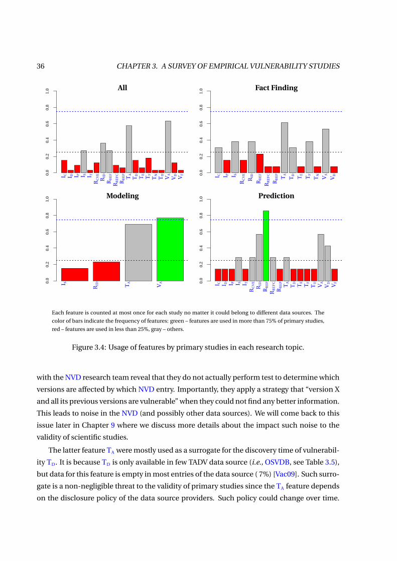
36 CHAPTER 3. A SURVEY OF EMPIRICAL VULNERABILITY STUDIES
All
0.0
0.2
0.4
0.6
0.8
1.0
I C I D I P I S I TR
CV
E
RID
RR
EF
RR
EF
C
RR
EP
TA
TD TE
TF
TN
TU VA
VD VF
Fact Finding
0.0
0.2
0.4
0.6
0.8
1.0
I C I P I SR
CV
E
RID
RR
EF
RR
EF
C
RR
EP
TA
TD TE
TF
TN VA
VD
Modeling
0.0
0.2
0.4
0.6
0.8
1.0
I S
RID T
A
VA
Prediction0.
00.
20.
40.
60.
81.
0
I C I D I P I S I TR
CV
E
RID
RR
EF
RR
EF
C
RR
EP
TA
TD TE
TF
TU VA
VD VF
Each feature is counted at most once for each study no matter it could belong to different data sources. The
color of bars indicate the frequency of features: green – features are used in more than 75% of primary studies,
red – features are used in less than 25%, gray – others.
Figure 3.4: Usage of features by primary studies in each research topic.
with the NVD research team reveal that they do not actually perform test to determine which
versions are affected by which NVD entry. Importantly, they apply a strategy that “version X
and all its previous versions are vulnerable” when they could not find any better information.
This leads to noise in the NVD (and possibly other data sources). We will come back to this
issue later in Chapter 9 where we discuss more details about the impact such noise to the
validity of scientific studies.
The latter feature TA were mostly used as a surrogate for the discovery time of vulnerabil-
ity TD. It is because TD is only available in few TADV data source (i.e., OSVDB, see Table 3.5),
but data for this feature is empty in most entries of the data source ( 7%) [Vac09]. Such surro-
gate is a non-negligible threat to the validity of primary studies since the TA feature depends
on the disclosure policy of the data source providers. Such policy could change over time.

3.4. CHAPTER SUMMARY 37
Thus it is very hard to approximate the discovery date by public announced date.
3.4 Chapter Summary
This chapter presented a survey about empirical vulnerability studies. The survey includes
59 primary studies in international workshops, conferences/symposium, and journals from
2005 to 2012. The survey studied the data sources and data features used in primary studies.
It also summarized most common features in the used data sources. The analysis on data us-
age has revealed that third-party data sources were preferred more than other data sources
to conduct empirical experiments. Among several data source, NVD was the most popular
one, which was used in about 62% of primary studies across different research topics. Ad-
ditionally, Affected Versions (VA) and Announced Date (TA) were the mostly used features in
primary studies.
In the next chapter, we will present the data infrastructure for compiling experimental
data which will be used in the rest of this dissertation.


CH
AP
TE
R
4DATA INFRASTRUCTURE FOR EMPIRICAL
EXPERIMENTS
This chapter focuses on the compilation of vulnerability data for further experiments
in the dissertation. It discusses the vulnerability data infrastructure including the
data sources and software infrastructure for data collection. It discusses potential bi-
ases in data sets that were collected based on the software infrastructure. The chapter
also describes other data sources such as market share information and code base
information of the target applications.
RECENTLY we have seen a substantial shift of vulnerability discovery from operating
systems to web browsers and their plugins [You13]. Additionally, a study by Google
[Raj11] shows that more than two-third of attacks to internet users have exploited
vulnerabilities of browsing software or its plugins. Therefore in this dissertation, we mostly
target our experiments on browsers, and select the most popular ones according to the main
providers of market share information.
Table 4.1 presents the vulnerability data sources for compiling the data infrastructure of
the dissertation. The category of the data source is based on the classification in the previ-
ous survey (see Table 3.2). The Apply for indicates the browsers of which the correspond-
ing data source provides vulnerability data. Among different third-party data sources (see
Table 3.3), we choose to use NVD because: first, it provides almost features which are sup-
ported by other third-party data sources; second, almost third-party data sources maintain
39

40 CHAPTER 4. DATA INFRASTRUCTURE FOR EMPIRICAL EXPERIMENTS
references to NVD; third, it is the most popular data source in the literature (see Section 3.3),
thus choosing NVD will enable us to compare the outcome of our experiments to the others.
The rest of this chapter is organized as follows. Section 4.1 presents the data sources as
well as the software infrastructure to collect vulnerability data. Section 4.2 discusses poten-
tial biases in the data set collected by the infrastructure, and how to mitigate them. Sec-
tion 4.3 describes how to obtain the market share data for browsers. Section 4.4 summarizes
the chapter.
4.1 Software Infrastructure for Data Acquisition
Vulnerability data is not static, but keeps evolving as more and more vulnerabilities are dis-
covered when time passes by. During the course of this dissertation we have to collect vul-
nerability data for several times, especially when we start new experiments so that we base
the experiments on the up-to-date data. Therefore, in this chapter we will not present any
snapshot of vulnerability data. Instead, we describe the software infrastructure to acquire
the data. This infrastructure is consistently used throughout all experiments within this dis-
sertation.
Moreover, from the perspective of researchers who are not inside the data source providers,
we are in favor of an automated process to collect vulnerability data. This makes the col-
lected data objective rather than subjective. Some sanitization activities could be applied
to the collected data to improve the quality. However these activities should be clearly de-
fined, and should not be subject to personal judgments, which could be different from per-
son to person. Therefore the experiments based on the data could be easily and widely re-
producible by other researchers.
Table 4.1: Vulnerability data sources of browsers.
Data Source Category Apply for
National Vulnerability Database (NVD) TADV All browsers
Mozilla Foundation Security Advisories (MFSA) ADV Firefox
Mozilla Bugzilla (MBug) BUG Firefox
Microsoft Security Bulletin (MSB) ADV IE
Apple Knowledge Base (AKB) ADV Safari
Chrome Issue Tracker (CIT) BUG Chrome

4.1. SOFTWARE INFRASTRUCTURE FOR DATA ACQUISITION 41
In the subsequent section we describe the software infrastructure to automate the data
acquisition task.
4.1.1 Acquiring Vulnerability Data for Firefox
Figure 4.1 exhibits the software infrastructure for collecting Firefox vulnerability data. The
infrastructure consists of a couple of scripts: Sphinx scripts (white rectangles) and R scripts
(filled rectangles). The former scripts are written in the Sphinx script language, which is
developed by myself and is optimized for extracting data in text files (e.g., HTML pages).
The latter scripts are written in R, a very popular language for data processing and statistics.
Apart from the output data set (stack of cans), the figure also shows some intermediate data
sources (filled cans), which are the outcome of the scripts.
The data collection process for Firefox starts by processing the MFSA dashboard (www.
mozilla.org/security/known-vulnerabilities/) which lists all MFSA entries. The MFSA
Feature Extractor invokes Web Crawler to download all HTML pages of all available MFSA
entries for Firefox, and parses the content of these pages to produce three intermediate data
sets: MFSA Data, MFSA Refs, and Bug-CVE Links. The first data set contains meta infor-
mation of each MFSA entry; the second maintains cross-reference links between an MFSA
entry to a CVE or an MBug entry; the third holds the associations between CVEs and MBugs
mentioned in each MFSA report.
For each MBug detected in an MFSA, MFSA Feature Extractor passes it to MBug Feature
MFSA
Firefox VDB
NVD
Feature Extractor
for Firefox
NVD Archives
Firefox
NVD
Data
Firefox
NVD
Refs
MBug
Sphinx
scripts
R
scripts
Intermediate
Data
Output Dataset
NVD
Archives
MFSA
Feature Extractor
Web CrawlerMBug
Feature Extractor
MFSA
Data
MFSA
Refs
MBug
Data
Firefox
Data Synthesizer
Control Flow
DataFlow
Bug-CVE
Links
Figure 4.1: The infrastructure to collect vulnerability data for Firefox

42 CHAPTER 4. DATA INFRASTRUCTURE FOR EMPIRICAL EXPERIMENTS
Extractor which in turn asks Web Crawler to download its corresponding XML page, and
parses the downloaded page to produce the data set MBug Data, which contains meta infor-
mation of MBug.
On the other side, NVD Feature Extractor for Firefox mines the NVD Archives data set,
which is provided by NVD (nvd.nist.gov/download.cfm), to produce two data sets: Fire-
fox NVD Data and Firefox NVD Refs. The former contains CVEs that mention Firefox as the
affected application. The latter maintains the all reference links of a CVE to either an MBug
or an MFSA entry. Finally all the intermediate data sets are fed into the Firefox Data Synthe-
sizer to produce the final output data set, Firefox VDB.
The schemas of all these data sets are described as follows:
MFSA Data = (mfsaID, mfsaDate, title)
MFSA Refs = (mfsaID, refType, refID)
Bug-CVE Links = (bugID, mfsaID, cveID, patternType)
MBug Data = (bugID, mfsaID, bugDate)
Firefox NVD Data = (cveID, cveDate, aectedVersion)
Firefox NVD Refs = (cveID, refType, refID)
Firefox VDB = (bugID, bugDate, mfsaID, mfsaDate,
cveID, cveDate, minAectedVersion, maxAectedVersion)
Some features are self-explained by their name, we only describe the meaning for the rest.
Particularly, refType is one of strings 'CVE', or 'Bugzilla', or 'MFSA', which indicates the
meaning of the refID feature. The feature patternType determines the heuristic rule used to
associate CVE and MBug.
The heuristic rules to associate CVE and MBug are based on the relative positions of the
hyperlinks to MBug and hyperlinks to NVD in an MFSA report. To clarify, we use the term
BUG and CVE to denote hyperlinks to MBugs, and CVEs, respectively. If more than one similar
term appears in a sequence, we use the star symbol (*). There are following cases for these
relative positions.
• BUG*: one or more MBug hyperlinks, see Figure 4.2(a). We thus have no clue to link
these MBug entries to any NVDs entries. However, this case only applies for Firefox
v1.0. Thus we can safely assume that these MBug entries only affect Firefox v1.0 be-
cause they are fixed in Firefox v1.0.x. In other words, we still obtain the missing values
for the IV feature.

4.1. SOFTWARE INFRASTRUCTURE FOR DATA ACQUISITION 43
(a) BUG* (b) BUG CVE
(c) CVE BUG* (d) BUG* CVE
Figure 4.2: Different patterns of BUG and CVE references in MFSA.

44 CHAPTER 4. DATA INFRASTRUCTURE FOR EMPIRICAL EXPERIMENTS
• BUG CVE: one MBug hyperlink followed by an NVD hyperlink, see Figure 4.2(b). We
assume that the mentioned MBug entry correlates to the mentioned NVD entry. We
then correlate these entries together. This case occurs in most MFSA entries.
• (CVE BUG*)*: one NVD entry is followed by one or more MBug entries, and then an-
other NVD entry and MBug entries, see Figure 4.2(c). We assume that the NVD entry
correlates to the immediately followed MBug entries.
• (BUG* CVE)*: this case is the opposite of the previous one, see Figure 4.2(d). There
is one or more MBug entries followed by an NVD entry, then other MBug entries and
another NVD entry. Similarly, we assume that MBug entries correlate to their followed
NVD entry.
By correlating NVD and MBug, we assume that all affected versions of the NVD entry are
also applied for the MBug entry.
4.1.2 Acquiring Vulnerability Data for Chrome, IE, and Safari
The software infrastructure to download vulnerability data for Chrome, IE and Safari is illus-
trated in Figure 4.3.
For Chrome, first we download the CIT Data data set which contains a list of security bugs
of Chrome. The GUI of CIT allows users to query the data. The queried results then could
be exported to Comma Separated Values (CSV) file. Since we are only interested in security
bugs, we set the query parameter to acquire only this type of bugs, i.e., type:Security-Bug.
Second, the NVD Feature Extractor for Chrome, as similar as NVD Feature Extractor for Fire-
fox, also mines the NVD Archives to produce two intermediate data sets Chrome NVD Data
and Chrome NVD Refs. The meaning of these two data sets are similar to Firefox NVD Data
and Firefox NVD Refs, which have been discussed above. Finally, all intermediate data sets
are fed into the Chrome Data Synthesizer to produce the final vulnerability data set for Chrome,
i.e., Chrome VDB.
The acquisition of vulnerability for IE and Safari are mostly the same as Chrome. In this
dissertation we have no interest in any features of MSB as well as AKB, except their IDs.
Therefore, we will not present the infrastructure to collect features form these data sources,
but only for collecting vulnerabilities for IE and Safari from the NVD Archives data set.
The schemas of the data sets in Figure 4.3 are described as follows.

4.2. POTENTIAL BIASES IN COLLECTED DATA SETS 45
Sphinx
scripts
R
scripts
Intermediate
Data
Output Dataset
Control Flow
DataFlow
CIT
Chrome VDB
CIT
Data
NVD
Feature Extractor
for Chrome
Chrome
NVD
Data
Chrome
NVD
Refs
Chrome
Data Synthesizer
Safari VDB
NVD
Feature Extractor
for Safari
NVD Archives
Safari
NVD
Data
Safari
NVD
Refs
Safari
Data Synthesizer
IE
Data Synthesizer
IE VDB
NVD
Archives
NVD
Feature Extractor
for IE
IE
NVD
Data
IE
NVD
Refs
Figure 4.3: The infrastructure to collect vulnerability data for Chrome, IE, and Safari.
CIT Data = (bugID, bugDate, cveID)
Chrome NVD Data = (cveID, cveDate, aectedVersion)
Chrome NVD Refs = (cveID, bugID)
IE NVD Data = (cveID, cveDate, aectedVersion)
IE NVD Refs = (cveID, msbID)
Safari NVD Data = (cveID, cveDate, aectedVersion)
Safari NVD Refs = (cveID, akbID)
Chrome VDB = (bugID, bugDate, cveID, cveDate,
minAectedVersion, maxAectedVersion)
IE VDB = (cveID, cveDate, msbID, minAectedVersion, maxAectedVersion)
Safari VDB = (cveID, cveDate, akbID, minAectedVersion, maxAectedVersion)
4.2 Potential Biases in Collected Data Sets
We have identified some validity threats to the collection of vulnerability data. These threats
are classified to the Construction validity to any experiments relying on this infrastructure to
attaining data. These threats are described as follows.

46 CHAPTER 4. DATA INFRASTRUCTURE FOR EMPIRICAL EXPERIMENTS
Bugs in the implementation scripts. The software infrastructure in Figure 4.1 and Fig-
ure 4.3 consists of some implemented scripts. These scripts might be buggy, leading to mis-
takes in the collected data. We have tried to remove programming bugs as much as possible.
We first ran all the scripts in some samples, and then manually check the outputs of these
scripts to see if there was any mistakes. If yes, we fixed the scripts and ran the test again.
When all identified bugs have been eliminated. We ran the scripts to collect all data sets.
Then we randomly sampled the data sets for mistakes. If there was any, we fixed the bugs
and started over the data collection.
Bias in correlating MBug to NVD entries. Some MBug entries explicitly indicate the cor-
responding NVD in their titles, but the most of them do not. We employ the heuristic rules
described in the previous section to link. The rules might not hold for all cases, leading to
mistakes in the collected data. We tried to mitigate the mistakes by manually checking the
description of MBug and NVD entries in some samples.
Figure 4.4 reports the distribution of number of MBugs per NVD entry reported by MFSA
entries (up to January 2014). In most of cases (86%), each NVD is associated with a sin-
gle MBug. This means that the associations between MBug and NVD established via MFSA
apparently contain less bias. However, we have still manually verified many correlations be-
tween NVD and MBug entries. Fortunately all of them are found consistent.
Example 4.1 This example illustrates the corresponding between NVD and MBug entries.
Number of MBugs per NVD entry
Den
sity
0.0
0.2
0.4
0.6
0.8
1.0
0.86
0.050.020.020.010.000.010.010.000.010.01
1 2 3 4 5 6 7 8 9 10 11+
Figure 4.4: Histogram of number of MBugs per NVD entry, reported by MFSA.

4.3. MARKET SHARE DATA 47
Figure 4.2(d) shows the screenshot of MFSA-2009-15. The description of this MFSA entry
said:
“Bjoern Hoehrmann and security researcher Moxie Marlinspike independently re-
ported that Unicode box drawing characters were allowed in Internationalized
Domain Names (IDN) where they could be visually confused with punctuation
used in valid web addresses. This could be combined with a phishing-type scam
to trick a victim into thinking they were on a different website than they actually
were.”
Also, this MFSA has two reference hyperlinks to two MBugs, and one reference hyperlink
to an NVD entry. The former are 479336 and 354592. The latter is CVE-2009-0652. The
description of the CVE-2009-0652 said:
“The Internationalized Domain Names (IDN) blacklist in Mozilla Firefox 3.0.6
and other versions before 3.0.9; Thunderbird before 2.0.0.21; and SeaMonkey be-
fore 1.1.15 does not include box-drawing characters, which allows remote attack-
ers to spoof URLs and conduct phishing attacks, as demonstrated by homoglyphs
of the / (slash) and ? (question mark) characters in a subdomain of a .cn domain
name, a different vulnerability than CVE-2005-0233. NOTE: some third parties
claim that 3.0.6 is not affected, but much older versions perhaps are affected.”
The titles of the MBug entries said:
MBug 479336: “ (CVE-2009-0652) IDN blacklist needs to include box-drawing
characters.”
MBug 354592: “Handling of U+2571 and U+FF1A in IDNs allows URL spoofing.”
By looking at the description of CVE-2009-0652 and the title of the two MBug 479336,
354592, it is clearly that they were talking about the same problem but at different levels of
abstraction.
4.3 Market Share Data
The information about market share of browsers are provided from several providers, e.g.,
Net Application (www.netmarketshare.com), StatCounter Global (gs.statcounter.com),
and W3Schools Online (www.w3schools.com/browsers/). Due to the lack of a standard way

48 CHAPTER 4. DATA INFRASTRUCTURE FOR EMPIRICAL EXPERIMENTS
Figure 4.5: The market share of browsers since Jan 2008.
to calculate software market share, these data providers use their own methods to achieve
the information. These methods could be classified into two classes: counting the number
of unique visitors (e.g., Net Application), or counting the number of page views (e.g., Stat-
Counter Global).
The latter method, counting the number of page views, might only be an approxima-
tion for the traffic share of browsers. This stats might be a good indicator for understanding
bandwidth-dominating browsers, but might be not appropriate for estimating the choice of
individual users which represents the market share. Since we are more interested in study-
ing the browser choice of individual people, we prefer to use the number of unique visitors
in this work.
Hereafter, we use the term market share to refer to the percentage of unique users of a
particular browser to the total unique users. Notably, users who interchangeably use more
than one browsers are counted multiple times.
We acquire market share of browsers from Net Application. The data is provided in
monthly percentage starting from January 2008 to September 2013. The market share of
each browser is the sum of all unique visitors (in percentage) of all versions of a browser. We
mostly focus on the share of top 4 dominant browsers. The market shares of these browsers
are exhibited in Figure 4.5.
Table 4.2 reports the yearly descriptive statistics of market shares of these browsers. All
the values are in percentage. The market share of Chrome in 2008 was below 1% because this
browser joint the market in December 2008.

4.4. CHAPTER SUMMARY 49
Table 4.2: Descriptive statistics of browsers market share.
Market share values are in percentage.
Year IE Firefox Chrome Safari
µ σ min max µ σ min max µ σ min max µ σ min max
2008 75.54 [2.38] 70.92 78.42 18.80 [1.67] 16.56 21.83 0.39 [0.58] 0.00 1.41 2.65 [0.19] 2.47 3.14
2009 67.55 [2.08] 63.69 70.17 23.54 [0.95] 22.27 25.05 2.68 [1.03] 1.53 4.71 3.52 [0.25] 3.19 3.88
2010 61.54 [1.07] 59.26 63.22 24.21 [0.67] 23.52 25.13 7.57 [1.49] 5.32 10.36 3.89 [0.08] 3.73 4.02
2011 55.87 [2.51] 51.87 59.22 22.67 [0.46] 21.83 23.72 14.60 [2.71] 11.15 19.11 4.63 [0.40] 4.13 5.43
2012 53.88 [0.59] 52.84 54.77 20.24 [0.38] 19.71 20.92 18.72 [0.59] 17.24 19.58 5.04 [0.23] 4.62 5.33
2013 56.30 [0.88] 55.14 57.80 19.57 [0.85] 18.29 20.63 16.58 [0.72] 15.74 17.76 5.46 [0.16] 5.24 5.77
4.4 Chapter Summary
This chapter presented the data infrastructure for the empirical experiments that will be dis-
cussed in the rest of the dissertation. We focused the data compilation for four browsers:
Chrome, Firefox, IE, and Safari. These browsers are top dominant in the market of browsing
software. The chapter described the software infrastructure for acquiring vulnerability data.
The chapter also presented the market share information for each browsers
In the next chapters, we are going to describe the observations based on the data col-
lected by the presented software infrastructure.


CH
AP
TE
R
5AFTER-LIFE VULNERABILITIES
This chapter reports our first observational study and studies the interplay in the
evolution of source code and known vulnerabilities in Firefox over six major versions
(v1.0–v3.6) spanning almost ten years of development. We observe a large fraction of
vulnerabilities apply to code that is no longer maintained in older versions. We call
these after-life vulnerabilities. Through an analysis of that code’s market share, we
also conclude that vulnerable code is still very much in use both in terms of instances
and as global code base: CVS evidence suggests that Firefox evolves relatively slowly.
PUBLIC vulnerability databases such as National Vulnerability Database (NVD, web.
nvd.nist.gov), Open Source Vulnerability Database (OSVDB, www.osvdb.org), Bug-
traq (www.securityfocus.com) have been used by both academics and industry to
study and assess the security of a software. Among these, NVD emerges as one of the most
popular source of vulnerabilities for a vast range of software types. Each entry in NVD (a.k.a
CVE) is assigned with a unique CVE-ID which has been used as a de-factor vulnerability
identifier among other vulnerability data sources. Each CVE is ‘assessed1’ against individual
versions (both older and recent ones) to understand which ones are vulnerable.
Besides the academic interests, the presence of “vulnerable" software, according to the
NVD, in a company’s deployment has a major impact on its compliance with regulation.
Some security protocol, such as US Government NIST SCAP [Qui10], evaluates the compli-
ance of software products based on the existence of vulnerabilities as well as their severity
1In fact, we do not known the assessment process.
51

52 CHAPTER 5. AFTER-LIFE VULNERABILITIES
score (e.g., CVSS). However, an analysis by Allodi and Fabio [AF12; All13b] on the exploits of
vulnerabilities in the wild has shown that basing on CVSS is not an effective strategy since
vulnerabilities with high CVSS score only represent a negligible amount of actual attacks.
Moreover, if you are a credit card merchant, you may need to obtain the compliance with
the PCI DSS[WC12] even if it is now not a regulation or a law2. If you use, e.g., Chrome v4
embedded in your products, then you might have a software that is vulnerable and may lose
the PCI DSS compliance since one of PCI DSS specific regulatory requirement is that: “fix all
medium- and high-severity vulnerabilities" [WC12, Chap. 9]. This may lead to fines raking
hundreds of thousands of euros.
Meanwhile the current strategy among software vendors is to counter the risk of exploits
by software evolution: security patches are automatically pushed to end customers, sup-
port for old versions is terminated, and customers are pressured to move to new versions.
The idea is that, as new software instances replace the old vulnerable instances, the eco-
system as a whole progresses to a more secure state. Additionally, this strategy also has some
economic advantages for software vendors: software market is a market of lemons [And01;
Ozm07b] the first comers have to change to gain market share, and the simultaneous main-
tenance of many old versions is simple too costly to continue. However such strategy leaves
many old, out-of-support versions, which we refer to as end-of-life versions – or simply dead
versions, with many unpatched vulnerabilities. This might be troubles for organizations who
still rely on end-of-life versions as discussed above.
The major concern that we try to address in this chapter is whether there is some empir-
ical evidence that software-evolution-as-a-security-solution is actually a solution, i.e., leads
to less vulnerable software over time.
The remainder of this chapter is structured as follows. Section 5.1 presents the findings
in the ecosystem of software evolution. Section 5.2 reports the findings in the ecosystem
of vulnerabilities. Section 5.3 analyzes the threats to validity. Section 5.4 summarizes the
chapter.
5.1 The Ecosystem of Software Evolution
We looked at six Firefox versions, namely v1.0, v1.5, v2.0, v3.0, v3.5 and v3.6. Their lifetimes
[Wik12a] can be seen from Figure 5.1. At the time of writing, the versions of Firefox that were
actively maintained were v3.5 and v3.6. Therefore, the rectangles representing version v3.5
2Some states in US (i.e., Nevada and Minnesota) have adopted PCI DSS as a actual law for some business
operating in these states [WC12, Chap.3 ]

5.1. THE ECOSYSTEM OF SOFTWARE EVOLUTION 53
and v3.6 actually extend to the right. There is very little overlap between two versions that
are one release apart, i.e., between v1.0 and v2.0, v1.5 and v3.0, v2.0 and v3.5, or v3.0 and
v3.6. This is consistent with the conscious effort by the Mozilla developers to maintain only
up to two versions simultaneously.
Figure 5.2 illustrates the evolution of Firefox code base from version v1.0 to v3.6. From
this figure, the large fraction of code re-use reconciliate the seemingly contradictory infor-
mation that vulnerability discovery is an hard process with the existence of zero-day at-
tacks: when a new release gets out, the 40% of old code have been already analyzed by over
6 months. Therefore the zero-day attack of version X could well be in reality a six month
mounting attack on version X-1.
There is a long held belief in the community that security exploits are a social phenomenon:
the wider a user base the more economic appeal it has as a target, the more vulnerabilities
are likely to be found. In order to evaluate the impact of social economic aspect of vulnera-
bilities we consider the market share of the various versions in order to calculate the attack
surface of code that is around. The intuition is to calculate the Line of Code (LoC) on each
version that are currently available to attackers, either by directly attacking that version or by
attacking the fraction of that version that was inherited in later versions.
Let users(v, t ) be the number of users of Firefox version v at time t , and let loc(p,c) be the
number of lines of code that the current version c has inherited from the previous version p.
Then the total number of lines of code in version c is∑
1≤p≤c loc(p,c). In order to get an idea
how much inherited code is used, we define a measure LOC-users as:
Lifetimes of Firefox Versions
2005 2006 2007 2008 2009 2010 2011
v1.0
v1.5
v2.0
v3.0
v3.5
v3.6
time
of o
bser
vatio
n
Figure 5.1: Release and retirement dates for Firefox.

54 CHAPTER 5. AFTER-LIFE VULNERABILITIES
V1.0 V1.5 V2.0 V3.0 V3.5 V3.6
Size and Lineage of Firefox Source Code
Version
Line
s of
Cod
e [m
illio
ns]
01
23
4
V1.0V1.5V2.0V3.0V3.5V3.6
V1.0 V1.5 V2.0 V3.0 V3.5 V3.6
Fraction of Inherited Code
Version
Fra
ctio
n of
Cod
e
0.0
0.2
0.4
0.6
0.8
1.0
V1.0V1.5V2.0V3.0V3.5V3.6
Evolution of Firefox codebase in absolute terms (left) and fraction of codebase (right). The left diagram shows
the size of the Firefox releases, and the right diagram normalizes all columns to a common height.
Figure 5.2: Size and lineage of Firefox source code
LOC-users(v, t ) = ∑1≤p≤v
users(p, t ) · loc(p, v). (5.1)
This is an approximation because the amount of code inherited into version v varies with
time, therefore, loc(p, v) is time-dependent. In this way, we eliminate transient phenomena
for this high-level analysis.
Figure 5.3 shows the development of the number of users and of LOC-users over time. It
is striking to see the number of Firefox v1.0 go down to a small fraction, while the LOC-users
for v1.0 stays almost constant.
An important observation is that even the “small” fraction of users of older versions ac-
counts to millions of users. You can imagine wandering in Belgium and each and every per-
son that you meet in the city still uses old Firefox v1.0.
This might have major implications in terms of the possibility of achieving herd immu-
nity as the number of vulnerable hosts would be always sufficient to allow propagation of
infections, see [Het00] for discussion on threshold for epidemics.

5.2. AFTER-LIFE VULNERABILITIES AND THE SECURITY ECOSYSTEM 55
2008 2009 2010 2011
Firefox Users
Year
Use
rs [m
illio
ns]
010
020
030
040
050
0
v1.0v1.5v2.0v3.0v3.5v3.6
2008 2009 2010 2011
Firefox LOC−Users
YearLO
C−
Use
rs [m
illio
ns]
050
010
0015
0020
00
V1.0V1.5V2.0V3.0V3.5V3.6
Number of Firefox users (left) and LOC-users (right). While the number of users of Firefox v1.0 is very small,
the amount of Firefox v1.0 code used by individual users is still substantial.
Figure 5.3: Firefox Users vs. LOC Users
5.2 After-life Vulnerabilities and the Security Ecosystem
We looked at security advisories of Firefox and found 335 MFSAs, from MFSA-2005-008 to
MFSA-2010-48. In order to find out in which version a vulnerability applies to, we look at the
NVD entry for a particular vulnerability and take the earliest version for which the vulner-
ability is relevant. For example, MFSA 2008-60 describes a crash with memory corruption.
This MFSA links to CVE 2008-5502, for which NVD asserts that versions v3.0 and v2.0 are
vulnerable. The intuitive expectation (confirmed by the tests) is that the vulnerability was
present already in v2.0 and that v3.0 inherited it from there.
Figure 5.4 exhibits the cumulative numbers of vulnerabilities in individual versions of
Firefox. In the figure, we additionally mark the end-of-life for each version by a vertical line.
As is apparent, the number continues to grow up even if the life time of a version is termi-
nated. We call vulnerabilities discovered after the life time of a version as after-life vulnera-
bilities.
By the time of this observation, Firefox v3.5 and v3.6 are alive. Obviously we have no
after-life vulnerabilities for them. However, for other versions, Figure 5.4 shows a significant
amount of after-life vulnerabilities in the security landscape of individual versions of Firefox.
This phenomenon could be explained by the ecosystem of code evolution, as previously

56 CHAPTER 5. AFTER-LIFE VULNERABILITIES
Number of Vulnerabilities in Firefox VersionsC
umul
ativ
e N
umbe
r of
Vul
nera
bilit
ies
010
020
030
040
050
0
2004 2006 2008 2010 2011
v1.0v1.5v2.0v3.0v3.5v3.6
Cumulative number of vulnerabilities for the various Firefox versions. End-of-life for a version is marked with
vertical lines. As is apparent, the number continues to rise even past a version’s end-of-life.
Figure 5.4: Vulnerabilities discovered in Firefox versions
presented in Figure 5.3. Even when a version is dead, their code base still survives for a very
long time since the code base is usually inherited across versions, see Figure 5.2. Thus when
a vulnerability is discovered in an alive version, i.e., a version which is still being supported,
it has some chances that this vulnerability falls into the code base of an older version, see
also Figure 5.2 (right). As the result, the number of after-life vulnerabilities arises.
After-life vulnerabilities are usually discovered in alive versions, then found to affect also
retro versions. In alive versions, these vulnerabilities are fixed and shipped to users through
security patches. However, they are not fixed in dead versions. Consequently, any products
relied on dead versions of Firefox would expose themselves to a major threat: they contain a
lot public-but-non-fixed after-life vulnerabilities.
We further study the breakdown of cumulative vulnerabilities in each version to see the
origin of vulnerabilities, i.e., where vulnerabilities were firstly introduced and survived. De-
pend on versions that a vulnerability affects, it can be classified into following sets:
• Inherited vulnerabilities are ones spanning consecutive versions.

5.2. AFTER-LIFE VULNERABILITIES AND THE SECURITY ECOSYSTEM 57
• Foundational vulnerabilities are inherited ones, but apply also for the very first version
e.g., v1.0.
• Local vulnerabilities are ones introduced in some versions, but fixed before the next
version comes out.
• Survive vulnerabilities are one discovered in some versions, and still survive in the next
versions.
• Regressive vulnerabilities are present in some versions, then they disappear to reappear
again in later versions.
This classification is obviously not exclusive. In the set of vulnerabilities of version x, the
inherited set I (x) subsumes foundational set F (x), and survive set of the immediate prede-
cessor S(x −1). Hence, if we categorize vulnerabilities of Firefox in general (do not consider
versions), we have three complete disjoint sets: foundational, non-foundational inherited,
and local vulnerabilities. Similarly, if we categorize vulnerabilities of each version individu-
ally, we have four disjoint sets: foundation, non-foundational inherited, survive, and local
vulnerabilities. In the collected vulnerability data, we observed a single instance of regres-
sive vulnerability, but it turned to be an input mistake which has been corrected later on by
the data provider.
The definition of foundational vulnerability is weaker (and thus more general) than the
one used by Ozment and Schechter [OS06]. We do not claim that there exists some code in
version v1.0 that is also present in, say, v1.5 and v2.0 when a vulnerability is foundational. For
us it is enough that the vulnerability applies to v1.0, v1.5 and v2.0. This is necessary because
many vulnerabilities (in the order of 20-30%) are not fixed. For those vulnerabilities it is
impossible, by looking at the CVS and Mercurial sources without extensive and bias-prone
manual analysis, to identify the code fragment from which they originated.
Table 5.1 reports the number of vulnerabilities in Firefox depended on the versions they
are discovered (columns), and the version they were first introduced (rows). For example,
there were 99 vulnerabilities that were discovered during the lifetime of Firefox v3.0, which
were introduced in Firefox v1.0. Since we have no regressions (see above), these 99 vulnera-
bilities also apply to all intermediate versions v1.5 and v2.0.
We can now easily categorize the vulnerabilities in the table according to the categories
that interest us: inherited vulnerabilities are the numbers above the diagonal (they are car-
ries over from some previous version); foundational vulnerabilities are those in the first row,

58 CHAPTER 5. AFTER-LIFE VULNERABILITIES
Table 5.1: Vulnerabilities in Firefox
Version at
Introduction
Version at Discovery
v1.0 v1.5 v2.0 v3.0 v3.5 v3.6
v1.0 79 72 33 99 34 61
v1.5 — 109 88 0 0 0
v2.0 — — 163 24 0 1
v3.0 — — — 64 30 5
v3.5 — — — — 34 49
v3.6 — — — — — 21
Table 5.2: Vulnerabilities in individual versions of Firefox
(a) All vulnerabilities
Inherited
from
Version
v1.0 v1.5 v2.0 v3.0 v3.5 v3.6
v1.0 378 299 227 194 95 61
v1.5 - 197 88 0 0 0
v2.0 - - 188 25 1 1
v3.0 - - - 99 35 5
v3.5 - - - - 83 49
v3.6 - - - - - 21
Total 378 496 503 318 214 137
(b) After-life vulnerabilities
Inherited
from
Version
v1.0 v1.5 v2.0 v3.0
v1.0 228 203 126 50
v1.5 - 1 0 0
v2.0 - - 1 0
v3.0 - - - -
v3.5 - - - -
v3.6 - - - -
Total 228 204 127 50
excluding the first element (they are carries over from version v1.0); local vulnerabilities are
those on the diagonal (they are fixed before the next major release and are not carried over).
Another interesting perspective is to look at vulnerabilities in individual versions. Ta-
ble 5.2(a) reports the cumulative numbers of individual versions of Firefox, and their break-
down. These number could be derived from Table 5.1. For example, the cumulative num-
ber of vulnerabilities for a particular version, e.g., v2.0, is the sum of cells (r ow,col ) where
r ow ≤ v2.0 and col ≥ v2.0, which is 503. For each version in the columns, numbers in the first
row (except version v1.0) are foundational vulnerabilities, numbers in the diagonal are sum
of local vulnerabilities and survive vulnerabilities, and others are non-foundational inherited
ones. Table 5.2(b) is similar to Table 5.2(a), but only after-life vulnerabilities are counted.
According to Table 5.2, among the total vulnerabilities in individual versions, on average,

5.3. THREATS TO VALIDITY 59
51% are inherited from the very first version – foundational vulnerabilities, 17% are inher-
ited from other versions. Intuitively, inherited vulnerabilities (both foundational and non-
foundational) are responsibility of the legacy code in each version. Hence, the contribution
of legacy code to the (in)security of software (Firefox) is still a large portion. It is coherent to
the large amount of legacy LoC in each version.
Substantially, about 40% of vulnerabilities have been discovered after the versions were
out of support. These after-life vulnerabilities are mostly foundational, see Table 5.2(b).
Considering the market share of Firefox, see Figure 5.3, there are a significant amount of
exploitable vulnerabilities in the ecosystem of Firefox.
In short, the observation based on the collected data has reveal the following finding
about the security landscape of Firefox.
“For each version of Firefox, foundational vulnerabilities take a significant amount
among the total vulnerabilities. More than one-third of vulnerabilities are after-
life i.e., discovered after a version were out of support, and most of them are foun-
dational."
5.3 Threats to Validity
Construct validity includes threats affecting the way we collect vulnerability data.
Bias in data collection. We apply the software infrastructure described in Chapter 4. As
discussed, it might have some construction validity to the observation in this chapter. We
inherit the mitigation described in Section 4.2 to reduce the bias in the collected data.
Bias in NVD. We determine the Firefox versions from which a vulnerability originated by
looking at the earliest Firefox version to which the vulnerability applies, and we take that
information from the “vulnerable versions” list in the NVD entry. If these entries are not re-
liable, we may have bias in the analysis. We have manually confirmed accuracy for few NVD
entries, and an automatic large-scale calibration will be a part of future work (considering
the time this observation were made). Indeed, we have done such calibration in Chapter 9
where we report the bias in NVD and revisit the findings in this observation.
Internal validity concerns the causal relationship between the collected data and the con-
clusion in the study.
Ignoring the severity. We deliberately ignore the severity of vulnerabilities in our study.
Because current severity scoring system, CVSS, adopted by NVD and other ones (e.g., quali-

60 CHAPTER 5. AFTER-LIFE VULNERABILITIES
tative assessment such as critical, moderate used in Microsoft Security Bulletin) have shown
their limitation. In accordance to Bozorgi et al. [Boz10], these systems are “inherently ad-hoc
in nature and lacking of documentation for some magic numbers in use". Moreover, in that
work, Bozorgi et al. showed that there is no correlation between severity and exploitability
of vulnerabilities.
External validity is the extent to which our conclusion could be generalized to other scenar-
ios. The combination of multi-vendor databases (e.g., NVD, Bugtraq) and software vendor’s
databases (e.g., MFSA, Bugzilla) only works for products for which the vendor maintains a
vulnerability database and is willing to publish it. Also, the source control log mining ap-
proach only works if the vendor grant community access to the source control, and devel-
opers commit changes that fix vulnerabilities in a consistent, meaningful fashion i.e., inde-
pendent vulnerabilities are fixed in different commits, each associated with a message that
refers to a vulnerability identifier. These constraints eventually limit the application of the
proposed approach.
Another facet of generality, which is also the limitation of this observation, is that whether
the findings are valid to other browsers, or other categories of software such as operating sys-
tem? We plan to overcome this limitation by extending the observation to different software
in future.
5.4 Chapter Summary
First, for the individual, we have the obvious consequence that running after-life software
exposes the user to significant risk, which should therefore be avoided. Also, we seem to
discover vulnerabilities late, and this, together with low software evolution speeds, means
that we will have to live with vulnerable software and exploits and will have to solve the
problem on another level.
Second, for the software ecosystem, the finding that there are still significant numbers of
people using after-life versions of Firefox means that old attacks will continue to work. This
means that the penetrate-and-patch model of software security (i.e., software-evolution-as-
a-security-solution) might not be enough, and that systemic measures, such as multi-layer
defenses, need to be considered to mitigate the problem.
These phenomena reveal that the problem of inherent vulnerabilities is merely a small
part of the problem, and that the lack of maintenance of older versions leave software (Fire-

5.4. CHAPTER SUMMARY 61
fox) widely open to attacks. Security patch is not made available because it is not being
deployed and because many users are slow at moving to newer version of software.
In terms of understanding the interplay of the evolution of vulnerabilities with the evo-
lution of software we think that the jury is still out, we cannot in any way affirm that most
vulnerabilities are due to foundational or anyhow past errors. We need to refine these find-
ings by a careful analysis of the fraction of the code base for each version.
These results have been possible by looking at vulnerabilities in a different way. Other
studies have studied a vulnerability’s past, i.e., once a vulnerability is known, we look at
where it was introduced, who introduced it etc. In this observation, we look at a vulnera-
bility’s future, i.e., we look at what happens to a vulnerability after it is introduced, and find
that it survives in after-life versions even when it is fixed in the current release.
The observation made in this chapter relies on the vulnerability claims by NVD. This
chapter assumes the data is all correctly provided. In Chapter 8, we present an automatic
method to estimate the retro persistence of vulnerability claims by NVD. Chapter 9 discusses
an experiment assessing the validity of vulnerability claims for Firefox and Chrome. The
experiment results exposes that many vulnerability claims for older versions of Chrome and
Firefox are not correct. Thus it might impact the observation of this chapter.
In the next chapter, we are going to present the observation on the traditional validation
methodology for vulnerability discovery models. The observation has revealed some critical
biases in the traditional methodology. Based on that, we have proposed a novel evaluation
methodology which can substitute the traditional one.


CH
AP
TE
R
6A METHODOLOGY TO EVALUATE
VULNERABILITY DISCOVERY MODELS
Vulnerability Discovery Models (VDMs) operate on known vulnerability data to es-
timate the total number of vulnerabilities that will be reported after software is re-
leased. This chapter presents an observation on the traditional validation method-
ology for VDMs. It discusses several issues which might bias the outcomes of valida-
tion experiments that follow the traditional methodology. Based on that, this chapter
proposes an empirical methodology that systematically evaluates the performance of
VDMs along two dimensions: quality and predictability. The proposed methodology
tackles all identified issues of the traditional methodology.
TIME-based vulnerability discovery models (VDMs) are parametric functions counting
the number of cumulative vulnerabilities of a software at an arbitrary time t . For
example, if Ω(t ) is the cumulative number of vulnerabilities at time t , the function
of the linear model (LN) is Ω(t ) = At +B where A,B are two parameters of LN, which are
calculated from the historical vulnerability data. Accurate models can be useful instruments
for both software vendors and users to understand security trends, plan patching schedules,
decide updates, and forecast security investments.
Figure 6.1 sketches a taxonomy of major VDMs. It includes Anderson’s Thermodynamic
(AT) model [And02], Rescorla’s Quadratic (RQ) and Rescorla’s Exponential (RE) models [Res05],
Alhazmi & Malaiya’s Logistic (AML) model [AM05b], AML for Multi-version (MVDM) model
63

64 CHAPTER 6. A METHODOLOGY TO EVALUATE VDMS
Vulnerability Discovery Models
Time-basedModels
Effort-basedModels
Quasi-LinearModels
SRGM-basedModels
S-shapeModels
Lin
ea
r (L
N)
Re
sco
rla's
Q
ua
rdra
tic (R
Q)
Re
scorla
's
Exp
on
en
tial
(RE
)
Lo
ga
rith
mic
Po
isso
n (
LP
)
An
de
rso
n's
Th
erm
od
yna
mic
(A
T)
Joh
's
We
ibu
ll (J
W)
Alh
azz
mi-
La
laiy
aL
og
istic
(A
ML
)
AM
L fo
r M
ulti
V
ers
ion
(M
VD
M)
Yo
un
is's
F
old
ed
(Y
F)
Effo
rt-b
ase
d
AM
LSRGM: Software Reliability Growth Model
Figure 6.1: Taxonomy of Vulnerability Discovery Models.
[Kim07], Weibull model (JW) [Joh08], and Folded model (YF) [You11]. Hereafter, we shortly
refer to time-based VDM as VDM.
The goodness-of-fit (GoF) of these models, i.e., how well a model could fit the numbers
of discovered vulnerabilities, is normally evaluated in each paper on a specific vulnerability
data set, except AML which has been validated for different types of applications (i.e., oper-
ating systems [Alh05; AM08], browsers [Woo06a], web servers [AM06b; Woo11]). Yet, all of
the validations so far have been done by the model authors, and there is no independent val-
idation by researchers who are different than these very authors. Furthermore, the validation
results of these studies might be biased by the following issues:
1. Past studies do not clearly define the notion of vulnerability. Indeed different defini-
tions of vulnerability (e.g., different databases such as NVD, versus MFSA) might lead
to different counted numbers of vulnerabilities, and consequently, different conclu-
sions.
2. All versions of a software are considered as a single entity. Though they belong to a

6.1. AN OBSERVATION ON THE TRADITIONAL VALIDATION METHODOLOGY 65
same product line, they are still different entities because they are different by a non-
negligible amount of code. Considering them as a single entity might make the valida-
tion results imprecise.
3. A model has been usually considered as a good fit to a data set if its goodness-of-fit test
returns p-value ≥ 0.05. This threshold is sound to reject a bad model, but it is overly
optimistic to conclude whether a model is good.
4. The goodness-of-fit of the models is often evaluated at a single time point (of writing
the paper). This could seriously impact the conclusion about the quality of a VDM be-
cause a VDM could obtain a good fit at a certain time point (i.e., horizon), but could
turn to be bad at another time point. For example, while fitting AML to Win2K vulnera-
bilities, the experiment in [Alh05] reported the significance level p-value = 0.44, which
could be positive; whereas p-value = 0.05 in [Alh07], which is bad. Moreover, no study
uses VDMs as a predictor, for example, to forecast data for the next quarter.
To deal with these issues, it is necessary to have a methodology that analyzes the perfor-
mance of VDMs independently and systematically. In this chapter we propose a methodol-
ogy that addresses these issues, and answers two questions concerning VDMs: “Are VDMs
adequate to capture the discovery process of vulnerabilities?", and “which VDM is the best?".
The rest of this chapter is organized as follows. Section ?? presents terminology in this
chapter. Section 6.1 discusses an observation on the traditional methodology for conduct-
ing validation experiments for VDMs in the literature. Section 6.3 summarizes the proposed
methodology in a nut shell. Section 6.4 details the proposed methodology. Section 6.5 sum-
marizes the chapter.
6.1 An Observation on the Traditional Validation
Methodology
This section describes an observation on the traditional validation methodology for VDMs
and past valuation experiments following that method. We separate the observation into two
parts. First, we summarize the previous studies on VDMs and the methodology that is em-
ployed to perform the validation. Second, we summarize the actual results of the validation
performed in past studies and discuss some critical issues.

66 CHAPTER 6. A METHODOLOGY TO EVALUATE VDMS
6.1.1 The Traditional Methodology
Table 6.1 summarizes VDM validation studies. Each study is reported with its target VDMs
and the classes of software applications used to conduct the experiment. The table also re-
ports the validation methodology of the studies. VDMs have been validated in several soft-
ware classes spanning from server applications, browsers, to operating systems. These stud-
ies shared a common validation methodology which fitted VDMs to a single time horizon of
collected vulnerability data. They used χ2 test to determine whether a VDM fits actual data.
If the test returned p-value ≥ 0.05, they claimed the VDM to be a good fit to the data.
Thus, we employ the χ2 test in our methodology because it yields comparable results
between traditional single horizon analysis and ours (when the horizon is restricted to be
unique). Furthermore, χ2 test seems to be the most appropriate one among other goodness-
of-fit tests, such as Kolmogorov-Smirnov (K-S) test, and the Anderson-Darling (A-D) test.
The K-S test is an exact test; it, however, only applies to continuous distributions. An im-
portant assumption is that the parameters of the distribution cannot be estimated from the
data. Hence, we cannot apply it to perform the goodness-of-fit test for a VDM. The A-D test
is a modification of the K-S test that works for some distributions [NIS12a, Chap. 1] (i.e., nor-
mal, log-normal, exponential, Weibull, extreme value type I, and logistic distribution), but
some VDMs violate this assumption.
Moreover, many VDM classifications of past studies claimed that a VDM is a good fit to a
data set when the χ2 test returns p-value ≥ 0.05 because 0.05 is the significance level to rule
out models that surely do not fit. However it does not mean the models are good. We avoid
this pitfall by using the acceptance threshold of 0.80, and rejection threshold of 0.05. Other-
wise, a VDM is inconclusive. We further discuss about these thresholds in Section 6.4.2. Ad-
ditionally, we propose inconclusiveness contribution factor ω as a means to study the quality
of inconclusive VDM in the quality analysis.
Some studies [AM05b; AM08] employed Akaike Information Criteria (AIC) [Aka85], which
measures the relative quality of a statistical model for a given data set, to compare VDMs.
However, AIC gives no information about the absolute quality. It thus cannot be used to
determine the goodness-of-fit of VDM. Moreover, AIC varies with the number of free param-
eters of a VDM. Consequently, it might not be a good indicator to compare VDMs, because a
model with more free parameters naturally grants an advantage in AIC. Therefore we do not
use AIC, but rely on statistic tests to determine the goodness-of-fit and compare VDMs.
The predictability of VDMs were also discussed in some studies [AM06b; Woo11; You11]
by exploiting two measures, namely Average Error (AE) and Average Bias (AB) [Mal92]. How-

6.1. AN OBSERVATION ON THE TRADITIONAL VALIDATION METHODOLOGY 67
Table 6.1: Summary of VDM validation studies.
Akaike Information Criteria (AIC) measures the relative quality of a statistical model for a given data set. Average Error (AE)
and Average Bias (AB) measure the average ratios between the actual data and the generated model.
Acronym: OS = operating system
Validation Method
Study Validated VDM Software Class Fit Model GoF test Predictability
Alhazmi et al.[Alh05] AML OS 1 horizon χ2 test –
Alhazmi et al.[AM05b] AML, AT, LP, RE, RQ OS 1 horizon χ2 test, AIC –
Alhazmi et al.[Alh07] AML, LN OS 1 horizon χ2 test –
Alhazmi et al.[AM06b] AML, LN Web Server 1 horizon χ2 test AE,AB
Alhazmi et al.[AM08] AML, AT, LN, LP, RE, RQ OS 1 horizon χ2 test, AIC –
Woo et al.[Woo06b] AML OS, Web Server 1 horizon χ2 test –
Woo et al.[Woo06a] AML Browser 1 horizon χ2 test –
Woo et al.[Woo11] AML OS, Web Server 1 horizon χ2 test AE,AB
Joh et al.[Joh08] AML, JW OS 1 horizon χ2 test –
Kim et al.[Kim07] AML, MVDM DBMS, Web Server 1 horizon χ2 test –
Younis et al.[You11] AML, YF Browser, OS, Web Server 1 horizon χ2 test AE,AB
Rescorla [Res05] RE, RQ OS 1 horizon unknown –
ever the application of AE and AB in these studies was inappropriate, because these mea-
sures were calculated for time points before the largest time horizon of the data set used
for fitting the VDMs. The authors used a VDM fitted to the data observed at time t0, and
measured its predictability at time ti < t0. In other words, this was not ‘prediction’ in the
common sense.
We avoid the above pitfall by analyzing the predictability of VDMs in a natural way. Con-
cretely, we fit a VDM to the data observed at time t0, and use the fitted model to evaluate
against data observed at time t j > t0.
6.1.2 The Validation Results of VDMs in Past Studies
Table 6.2 summarizes the validation results for VDMs. This table reports the p-values re-
turned by the goodness-of-fit test between generated curves and actual data. In Table 6.2,
p-values greater than or equal 0.80 (i.e., good fit) are bold, p-values between 0.05 and 0.80
(i.e., inconclusive-fit) are italic, otherwise it is a not-fit.
The AML model, inspired by the s-shape logistic model, is proposed by Alhazmi and
Malaiya [AM05b]. The idea behind is to divide the discovery process into three phases: learn-

68 CHAPTER 6. A METHODOLOGY TO EVALUATE VDMS
Table 6.2: Summary of VDM validation results (p-values) in the literature.
This table reports the returned p-values for the goodness-of-fit tests. The values are formatted to indicate the goodness-of-
fit of the VDM, particularly: blue,bold-good fit; italic-inconclusive; red-not fit.
Mo
del
Stu
dy
Year
Fir
efox
IE IE8
Moz
illa
MyS
QL
Free
BSD
4.0
OSX
5
RH
Fed
ora
RH
Lin
ux
6.0
RH
Lin
ux
6.2
RH
Lin
ux
7.0
RH
Lin
ux
7.1
RH
EL
2.1
RH
EL
3.0
Win
2K3
Win
2K
Win
7W
in95
Win
98
Win
NT
4.0
Win
XP
Ap
ach
eA
pac
he
1A
pac
he
2II
SII
S4
IIS
5
AML [Alh05] 2005 0.44 1 0.74 0.92 0.96
[AM05b] 2005 1 1 0.92
[Alh07] 2006 1 0.99 0.05 1 0.21 0.92 0.32
[AM06b] 2006 1 1 1 1
[Woo06b] 2006 1 1 1 1
[Woo06a] 2006 0.41 0 1
[Kim07] 2007 0.99 1
[AM08] 2008 0.43 1 1 0.15
[Joh08] 2008 0.81 0.85 0.83 0.66 0.96 0.94
[Woo11] 2011 1 0.65 1 1
[You11] 2011 0.73 0.98 0.70 1
AT [AM05b]∗ 2005 0 0 0
[AM08]∗ 2008 0 0 0 0
JW [Joh08] 2008 0.80 0.85 0.81 0.64 0.97 0.94
LN [Alh07]∗ 2006 0.93 0 1 0 0.95 0 0.08
[AM06b]∗ 2006 0 1 0 0.23
[AM08]∗ 2008 0 0 0 0
LP [AM05b]∗ 2005 1 0 0.97
[AM08]∗ 2008 0 0 0 0
RE [AM05b]∗ 2005 0.93 0 0.96
[Res05] 2005 0.29 0.33
[AM08]∗ 2008 0 0 0 0
RQ [AM05b]∗ 2005 0.92 0 1
[Res05] 2005 0.17 0.17 0.59
[AM08]∗ 2008 0 0.26 0 0.97
YF [You11] 2011 0.98 0.94 0.97 1
∗: the validation experiment is conducted by people who are not (co-)authors of the corresponding model.
ing phase, linear phase, and saturation phase. First, people need time to study the software,
so they discover less vulnerabilities. Second, when they understand the software, they can
discover more vulnerabilities. Finally, people lose interest in finding vulnerabilities when
the software is out of date. So cumulative vulnerabilities tend to be stable. However, the ob-
servation in Chapter 5 showed that this idea might not hold as vulnerabilities found for the
current version usually affect also earlier ones thus generating an increase of so-called “after-

6.2. RESEARCH QUESTIONS 69
life" vulnerabilities1. Nonetheless, we still adopt their idea in the proposed methodology by
dividing software life time into three periods: young, middle-age, and old.
The AML model has been validated in several applications spanning in various software
classes, see Table 6.2, such as operating systems [Alh05; AM05b; Alh07; AM08], server ap-
plications [AM06b; Woo06b; Woo11], and browsers [Woo06a]. In most cases, AML was ei-
ther inconclusive-fit or good-fit. Notably, the goodness-of-fit of AML was different for the
same application across different studies. For instance, AML well fitted Win98 in [Woo06b;
Woo11] (p-value = 1), but inconclusively fitted Win98 in [Alh05] (p-value = 0.74) and [Alh07]
(p-value = 0.21). The difference between p-values in these experiments is non-negligible.
Such difference can be explained by the validation methodology based on a single horizon.
This is a clear evidence that goodness-of-fit of a model is changing overtime. Thus, fitting a
model to a single time horizon is potentially misleading. We cope with this issue by analyzing
the VDM goodness-of-fit during the entire life time of software.
Anderson [And02] proposed the AT model based on reliability growth models, but he did
not evaluate it. Other studies [AM05b; AM08] showed that AT is not appropriate.
Rescorla [Res05] proposed RQ and RE models. He validated them on WinNT 4.0, Solaris
2.5.1, FreeBSD 4.0 and RedHat 7.0. In all cases, the goodness-of-fit of these models were in-
conclusive since their p-value ranged from 0.17 to 0.59. Rescorla also discussed many short-
comings of NVD, but his study heavily relied on it nonetheless. We partially address these
shortcomings by taking into account other data sources.
6.2 Research Questions
In this chapter, we address the two following questions:
RQ3 How to evaluate the performance of a VDM?
RQ4 How to compare between two or more VDMs?
In order to satisfactorily answer the questions above, we must address the following is-
sues that potentially affected the validity of previous studies.
Vulnerability counting issue. This issue affected the vulnerability data collection process in
past studies. The issue has two folds: what counted as one vulnerability, and what considered
as one vulnerable software.1After-life vulnerabilities of a version are ones discovered after the date when this version is out of support,
see also Chapter 5.

70 CHAPTER 6. A METHODOLOGY TO EVALUATE VDMS
• In the first fold, a vulnerability could be either an advisory report by software vendors
(e.g., MFSA), or a security bug causing software to be exploited (e.g., Mozilla Bugzilla),
or an entry in third-party data sources (e.g., an NVD entry, or CVE, alternatively). Some
entries may be classified differently by different entities: a third-party database might
report vulnerabilities, but the vendor security bulletin may not classify them as such.
Consequently, the number of vulnerabilities could be widely different depending on
the way of counting vulnerabilities, for instance, choosing different data sources. A
VDM could perfectly fit counts in a data source, but poorly fit counts in another one.
• In the second fold, some studies (e.g., [Woo06a; Woo11]) considered all versions of soft-
ware as a single entity, and counted vulnerabilities for it. Our previous study [Mas11]
showed that each Firefox version has its own code base, which may differ by 30% or
more from the immediately preceding one. The same applies to Chrome2. Another
example, Joh et al. [Joh08], in their experiment, showed that AML and JW curves fitted
for the ‘single’ Linux (i.e., all versions of Linux as a single entity), and those fitted for in-
dividual Linux versions (i.e., v6.0, v6.2) were utterly statistically different. Therefore, as
time goes by, we can no longer claim that we are counting vulnerabilities of the same
application.
Example 6.1 Figure 6.2(a) exemplifies the first fold of this issue, where a conceptual security
flaw could be counted differently if different data sources were used. This flaw concerns the
buffer overflow in Firefox v13.0. It is reported by: 1 entry in MFSA (MFSA-2012-40), 3 entries
in Bugzilla (744541, 747688, and 750066), and 3 CVEs in NVD (CVE-2012-1947, CVE-2012-
1940, and CVE-2012-1941). The cross references between these entries are illustrated as
directional connections. How many vulnerabilities should we count in this case?
Figure 6.2(b) visualizes the second fold of this issue in a plot of the cumulative vulnerabil-
ities of Firefox v1.0, Firefox v1.5, and Firefox v1.0-1.5 as a single entity. Clearly, the function
of the “global" version should be different from the functions of the individual versions.
Table 7.3 later in the next chapter shows how the choice of the counting method has
a massive impact on the results: by using the NVD alone, LN scores 45% of not-fit samples
(third-worst), while the YF model makes a 55% of good fits (best of all). However, by counting
the number of bugs correlated with number of NVD entries, i.e., NVD.NBug, the roles are
2By looking at the source code of Chrome (http://dev.chromium.org/Home), we found that after one
year the number of new components (i.e., body and header C++ files) increases more than 100%.

6.2. RESEARCH QUESTIONS 71
MFSA
Bugzilla
NVD
MFSA-2012-40
CVE-2012-1940
CVE-2012-1941
744541
747688
750066
CVE-2012-1947
The arrow-headed lines indicates the cross-
references between entries.
(a) A conceptual security flaw in three data sources
0 10 20 30 40
050
100
150
200
250
Months since released date
Cum
ulat
ive
num
ber
of v
ulne
rabi
litie
s
FF 1.0FF 1.5FF 1.0−1.5
This shows the cumulative vulnerabilities of Fire-
fox v1.0, v1.5, and v1.0-v1.5 as a single entity. The
“global" entity exhibits a trend that is not present
in the “individual" versions.
(b) Trends between individual versions and their combination
Figure 6.2: The two folds of the vulnerability counting issue.
reversed: LN exhibits a 41% of good fits (second bests), while YF shows a disastrous 50% of
not-fit samples (fourth worst).
Acceptance threshold issue. This issue affected the decision of past studies whether a model
was a good fit, or a bad fit to a data set based on the result of the χ2 test. Most of past studies
concluded a model was a good fit if the χ2 test returned p-value ≥ 0.05. However, 0.05 is the
threshold to reject a surely bad model. Yet, there is a long stretch from concluding that a
model is not surely a bad one to concluding that it is surely a good one.
Temporal goodness-of-fit issue. This issue impacted the ability of VDMs to explain history.
Previous studies took a snapshot of vulnerability data, and fitted VDMs to this entire snap-
shot. This made a brittle claim of fitness. Moreover, it could explain historical data but told
us nothing about future behavior. Yet, we are interested in the ability of VDMs to be a good

72 CHAPTER 6. A METHODOLOGY TO EVALUATE VDMS
“law of nature" that is valid across releases and time and to some predict extent the future.
Example 6.2 In Table 6.2, the p-values that AML fitted Win2K vulnerabilities in [Alh05;
Alh07] were 0.44 and 0.05, respectively. While the former is inconclusive, the latter is at the
border of rejection i.e., not fit. This is explained because AML was fitted to data sets at two
different time horizons in these experiments.
Comparison issue. This issue impacted the way past studies used to compare VDMs, where
comparison was relied directly on the absolute p-values yielded by the goodness-of-fit test.
The rule was: the higher p-value, the better model. However, the literature has shown that
such p-values have been changing over time, see Table 6.2. As a result, we might obtain
opposite conclusion if we compare VDMs at different time points.
6.3 Methodology Overview
We propose a methodology (see Table 6.3) to answer these questions. The methodology con-
sists of data collection and analysis steps to empirically assess different aspects of VDMs. It
addresses all above issues as follows:
• We address the vulnerability counting issue by considering different counting methods
on different vulnerability data sources. Hence, the performances of VDMs are evalu-
ated on average.
Moreover, we evaluate VDMs on vulnerability data of individual releases of evolving
applications, instead of considering all releases of an application as a single entity. The
rationale for this choice is discussed later in Section 6.4.1.
• We address the acceptance threshold issue by employing the Type-II error threshold
(i.e., 0.80) which is an considered desirable threshold [McK05, Chap.8] for the power
of the χ2 test to decide whether an estimated model is a good fit. We also use the
Type-I error threshold (i.e., 0.05) to reject models since it is widely used in not only the
literature, but also other disciplines.
• We mitigate the temporal goodness-of-fit issue by essentially analyzing the goodness-
of-fit of VDMs monthly until the date of data collection, instead of taking an arbitrary
time point in the lifetime of software. We also examine the ability of VDMs in predict-
ing the future trend.

6.3. METHODOLOGY OVERVIEW 73
• We address the comparison issue by using statistical tests to compare VDMs based on
their quality of fitting historical data and their predictability of future trends.
Table 6.3: Methodology overview.
Step 1 Acquire the vulnerability data
DESC. Identify the vulnerability data sources, and the way to count vulnerabilities.
If possible, different vulnerability sources should be used to select the most
robust one. Observed samples then can be extracted from collected vulnera-
bility data.
INPUT Vulnerability data sources.
OUTPUT Set of observed samples.
CRITERIA CR1 Collection of observed samples
• Vulnerabilities should be counted for individual releases (possibly by
different sources).
• Each observable sample should have at least 5 data points.
Step 2 Fit the VDM to observed samples
DESC. Estimate the parameters of the VDM formula to fit observed samples as much
as possible. The χ2 goodness-of-fit test is employed to assess the goodness-
of-fit of the fitted model based on criteria CR2.
INPUT Set of observed samples.
OUTPUT Set of evaluated samples.
to be continued...

74 CHAPTER 6. A METHODOLOGY TO EVALUATE VDMS
Table 6.3: Methodology overview (continued).
CRITERIA CR2 The classification of the evaluated samples based on the p-value of a χ2
test.
• Good Fit: p-value ∈ [0.80,1.0], a good evidence to accept the model. We
have more than 80% chances of generating the observed sample.
• Not Fit: p-value ∈ [0,0.05), a strong evidence to reject the model. It
means less than 5% chances that the fitted model would generate the
observed sample.
• Inconclusive Fit: p-value ∈ [0.05,0.80), there is not enough evidence to
neither reject nor accept the fitted model.
Step 3 Perform goodness-of-fit quality analysis
DESC. Analyze the goodness-of-fit quality of the fitted model by using the temporal
quality metric which is the weighted ratio between fitted evaluated samples
(both Good Fit and Inconclusive Fit) and total evaluated samples.
INPUT Set of evaluated samples.
OUTPUT Temporal quality metric.
CRITERIA CR3 The rejection of a VDM.
A VDM is rejected if it has a temporal quality lower than 0.5 even by counting
Inconclusive Fits samples as positive (with weight 0.5). Different periods of
software lifetime could be considered:
• 12 months (young software)
• 36 months (middle-age software)
• 72 months (old software)
Step 4 Perform predictability analysis
to be continued...

6.3. METHODOLOGY OVERVIEW 75
Table 6.3: Methodology overview (continued).
DESC. Analyze the predictability of the fitted model by using the predictability met-
ric. Depending on different usage scenarios, we have different observation
periods and time spans that the fitted model supposes to be able to predict.
This is described in CR4.
INPUT Set of evaluated samples.
OUTPUT Predictability metric.
CRITERIA CR4 The observation period and prediction time spans based on some possible
usage scenarios.Observation Prediction
Scenario Period (months) Time Span (months)
Short-term planning 6–24 3
Medium-term planning 6–24 6
Long-term planning 6–24 12
Step 5 Compare VDM
DESC. Compare the quality of the VDM with other VDMs by comparing their tem-
poral quality and predictability metrics.
INPUT Temporal quality and predictability measurements of models in comparison.
OUTPUT Ranks of models.
CRITERIA CR5 The comparison between two VDM
A VDM vdm1 is better than a VDM vdm2 if:
• either the predictability of vdm1 is significantly greater than that of
vdm2,
• or there is no significant difference between the predictability of vdm1
and vdm2, but the temporal quality of vdm1 is significantly greater than
that of vdm2.
The temporal quality and predictability should have their horizons and pre-
diction time spans in accordance to criteria CR3 and CR4. Furthermore, a
controlling procedure for multiple comparisons should be considered.

76 CHAPTER 6. A METHODOLOGY TO EVALUATE VDMS
6.4 Methodology Details
This section discusses the details of our methodology to evaluate the performance of a VDM.
6.4.1 Step 1: Acquire the Vulnerability Data
The acquisition of vulnerability data consists of two sub steps: Data set collection, and Data
sample extraction.
During Data set collection, we identify data sources for the study. The classification of
data sources is presented in Table 3.2. For our purposes, the following features of a vulnera-
bility are interesting and must be provided:
• Unique ID (RID): is the identifier of a vulnerability.
• Discovery Date (TD): refers to the date when a vulnerability is reported to the database3.
• Affected Versions (VA): is a list of releases affected by a vulnerability.
• Reference Links (RREF): is a list of links to other sources.
Not every feature is available from all data sources. To obtain missing features, we can use
RID and RREF to integrate data sources and extract the expected features from secondary data
sources.
Example 6.3 Vulnerabilities of Firefox are reported in three data sources: NVD4, MFSA, and
Mozilla Bugzilla. Neither MFSA nor Bugzilla provides the Affected Versions feature, but NVD
does. Each MFSA entry has links to NVD and Bugzilla. Therefore, we could to combine these
data sources to obtain the missing data.
We address the vulnerability counting issue issue by taking into account different defi-
nitions of vulnerability. We collected different vulnerability data sets with respect to these
definitions. We collected vulnerability data for individual releases. Table 6.4 shows different
data sets in this work. They are combinations of data sources : third-party (i.e., NVD), ven-
dor advisory, and vendor bug tracker. The descriptions of these data sets for a release r are
as follows:
3The actual discovery date might be significantly earlier.4Other third party data sources (e.g., OSVDB, Bugtraq, IBM XForce) also report Firefox’s vulnerabilities, but
most of them refer to NVD by the CVE-ID. Therefore, we consider NVD as a representative of third-party data
sources.

6.4. METHODOLOGY DETAILS 77
Table 6.4: Formal definition of data sets.
Data set Definition
NVD(r ) nvd ∈NVD|r ∈ nvd.VA
NVD.Bug(r ) nvd ∈NVD|∃b ∈BUG : r ∈ nvd.VA ∧b.RID ∈ nvd.RREF
NVD.Advice(r ) nvd ∈NVD|∃a ∈ADV : r ∈ nvd.VA ∧a.RID ∈ nvd.RREF
NVD.NBug(r ) b ∈BUG|∃nvd ∈NVD : r ∈ nvd.VA ∧b.RID ∈ nvd.RREF
Advice.NBug(r ) b ∈BUG|∃a ∈ADV,∃nvd ∈NVD : r ∈ nvd.VA ∧b.RID ∈ a.RREF ∧nvd.RID ∈ a.RREF∧clustera(b.RID,nvd.RID)
Note: nvd.VA ,nvd.RREF denote the vulnerable releases and references of an entry nvd, respectively. a.RID ,b.RID ,nvd.RID
denote the identifier of a, b, and nvd. clustera(b.RID ,nvd.RID) is a predicate checking whether b.RID and nvd.RID are located
next together in the advisory a.
• NVD(r): a set of CVEs claiming r is vulnerable.
• NVD.Bug(r): a set of CVEs confirmed by at least a vendor bug report, and claiming r is
vulnerable.
• NVD.Advice(r): a set of CVEs confirmed by at least a vendor advisory, and claiming r is
vulnerable. Notice that the advisory report might not mention r , but later releases.
• NVD.Nbug(r): a set of vendor bug reports confirmed by a CVE claiming r is vulnerable.
• Advice.NBug(r): a set of bug reports mentioned in a vendor advisory report, which also
refers to at least a CVE that claims r is vulnerable.
We do not use the NVD alone in our studies. We will later show in Chapter 9 that it may
contain significant errors to the point of tilting statistical conclusions.
For Data sample extraction, we extract observed samples from collected data sets. An
observed sample is a time series of (monthly) cumulative vulnerabilities of a release. It starts
from the first month since release to the end month, called horizon. A month is an appro-
priate granularity for sampling because week and day are too short intervals and are subject
to random fluctuation, see also [Sch09a] for a discussion. Additionally, this granularity was
used in the literature (e.g., studies listed in Table 6.1).
Let R be the set of analyzed releases and DS be the set of data sets, an observed sample
(denoted as os) is a time series (ts) defined as follows:
os= TS(r,d s,τ) (6.1)
where:

78 CHAPTER 6. A METHODOLOGY TO EVALUATE VDMS
• r ∈ R is a release in the evaluation;
• d s ∈ DS is the data set where samples are extracted;
• τ ∈ Tr =[τr
mi n ,τrmax
]is the horizon of the observed sample, in which Tr is the horizon
range of release r .
In the horizon range of release r , the minimum value of horizon τrmi n of r depends on the
starting time of the first observed sample of r . Here we choose τrmi n = 6 for all releases so
that all observed samples have enough data points for fitting all VDMs. The maximum value
of horizon τrmax depends on how long the data collection period is for each release.
Example 6.4 IE v4.0 was released in September, 1997 [Wik12b]. The first month was Octo-
ber, 1997. The first observed sample of IE v4.0 is a time series of 6 numbers of cumulative
vulnerabilities for the 1st ,2nd , . . . ,6th months. Starting data collection on 01st July 2012, IE
v4.0 would have been released for 182 months, yielding 177 observed samples. The maxi-
mum value of horizon (τIEv4.0max ) is 182.
6.4.2 Step 2: Fit a VDM to Observed Samples
We estimate the parameters of the VDM formula by a regression method so that the VDM
curve fits an observed sample as much as possible. We denote the fitted curve (or fitted
model) as:
vdmTS(r,d s,τ) (6.2)
where vdm is the VDM being fitted; os = TS(r,d s,τ) is an observed sample from which the
vdm’s parameters are estimated. (6.2) could be shortly written as vdmos.
Example 6.5 Fitting the AML model to the NVD data set of Firefox v3.0 at the 30th month,
i.e., the observed sample os = TS(FF3.0,NVD,30), generates the curve:
AMLTS(FF3.0,NVD,30) =183
183 ·0.078 ·e−0.001·183·t +1
Figure 6.3 illustrates the plots of three curves AMLTS(r,NVD,30), where r is FF3.0,FF2.0, and
FF1.0. The X-axis shows months since release, and the Y-axis is the cumulative number of
vulnerabilities. Circles represent observed vulnerabilities. Solid lines indicate fitted curves.

6.4. METHODOLOGY DETAILS 79
0 5 10 15 20 25 30
50
100
150
200
Firefox 3.0/nvd
ObservedAML [Fit]
0 5 10 15 20 25 30
50
100
150
Firefox 2.0/nvd
ObservedAML [Inconclusive]
0 5 10 15 20 25 30
020
40
60
80
100
120
Firefox 1.0/nvd
ObservedAML [Not Fit]
A = 0.001
B = 183
C = 0.078
A = 4.7e-4
B = 235.4
C = 0.037
A = 0.002
B = 117.1
C = 0.107
Month Since Release
Cu
mul
ativ
e V
uln
erab
iliti
es
p-value = 0.0001p-value = 0.417p-value = 0.993
A,B,C are three parameters in the formula of the AML model: Ω(t ) = BBCe−AB t+1
(see also Table 7.2)
Figure 6.3: Fitting the AML model to the NVD data sets for Firefox v3.0, v2.0, and v1.0.
In Figure 6.3, the distances of the circles to the curve are used to estimate the goodness-
of-fit of the model. To measure the goodness-of-fit, we employ Pearson’s Chi-Square (χ2) test
as aforementioned in Section 6.1. In this test, we calculate the χ2 statistic value of the curve
by using the following formula:
χ2 =τ∑
t=1
(Ot −Et )2
Et(6.3)
where Ot is the observed cumulative number of vulnerabilities at time t (i.e., t th value of the
observed sample); Et denotes the expected cumulative number of vulnerabilities which is
the value of the curve at time t . The χ2 value is proportional to the differences between the
observed values and the expected values. Hence, the larger χ2, the smaller goodness-of-fit.
If the χ2 value is large enough, we can safely reject the model. In other words, the model
statistically does not fit the observed data set. The χ2 test requires all expected values be at
least 5 to ensure the validity of the test [NIS12a, Chap. 1]. If there is any expected value less
than 5, we need to increase the starting value of t in (6.3) until Et ≥ 5.
The conclusion whether a VDM curve statistically fits an observed sample relies on the p-
value of the test, which is derived from χ2 value and the degrees of freedom (i.e., the number
of months minus one). Semantically, the p-value is the probability that we falsely reject the
null hypothesis when it is true (i.e., error Type I: false positive). The null hypothesis used
in past research paper is that “the model fits the data." [Alh07, page 225]. Therefore, if the
p-value is less than the significance level α of 0.05, we can reject a VDM because there is less
than 5% chances that this fitted model would generate the observed sample. This provides

80 CHAPTER 6. A METHODOLOGY TO EVALUATE VDMS
us a robust test to discard a model.
To accept a VDM, we exploit the power of the χ2 test which is the probability of rejecting
the null hypothesis when it is false. Normally, ‘an 80% power is considered desirable’ [McK05,
Chap. 8]. Hence we accept a VDM if the p-value is greater than or equal to 0.80. We have more
than 80% chances of generating the observed sample from the fitted curve. In other cases,
we should neither accept nor reject the model (inconclusive fit).
The criteria CR2 in Table 6.3 summarizes the assessment the goodness-of-fit based on
the p-value of the χ2 test.
In the sequel, we use the term evaluated sample to denote the triplet composed by an
observed sample, a fitted model, and the p-value of the χ2 test.
Example 6.6 In Figure 6.3, the first plot shows the AML model with a Good Fit (p-value =0.993 > 0.80), the second plot exhibits the AML model with an Inconclusive Fit (0.05 < p-value =0.417 < 0.80), and the last one denotes the AML model with a Not Fit (p-value = 0.0001 <0.05). To calculate the χ2 test we refit the model each and every time. So we have 1,526 dif-
ferent parameters A, B and C for each good fit curve (see Figure 6.3). Notice how each set
of parameters is widely different. If we used the same parameters for different versions, we
would rarely obtain a good fit.
6.4.3 Step 3: Perform Goodness-of-Fit Quality Analysis
We introduce the goodness-of-fit quality (or quality, shortly) by measuring the overall num-
ber of Good Fits and Inconclusive Fits among different samples. Previous studies considered
only one observed sample in their experiment, the one with the largest horizon.
Let OS = TS(r,d s,τ)|r ∈ R ∧d s ∈ DS ∧τ ∈ Tr be the set of observed samples, the overall
quality of a model vdm is defined as the weighted ratio of the number of Good Fit and In-
conclusive Fit evaluated samples over the total ones, as shown:
Qω = |GES|+ω · |IES||ES| (6.4)
where:
• ES = ⟨os,vdmos, p
⟩ |os ∈ OS
is the set of evaluated samples generated by fitting vdm
to observed samples;
• GES = ⟨os,vdmos, p
⟩ ∈ ES|p ≥ 0.80
is the set of Good Fit evaluated samples;
• IES = ⟨os,vdmos, p
⟩ ∈ ES|0.05 ≤ p < 0.80
is the set of Inconclusive Fit evaluated sam-
ples;

6.4. METHODOLOGY DETAILS 81
• ω ∈ [0..1] is the inconclusiveness contribution factor denoting that an Inconclusive Fit
is ω times less important than a Good Fit.
The overall quality metric ranges between 0 and 1. The quality of 0 indicates a completely
inappropriate model, whereas the quality of 1 indicates a perfect one. This metric is a very
optimistic measure as we are essentially “refitting" the model as more data become available.
Hence, it is an upper bound value.
The factorω denotes the contribution of an inconclusive fit to the overall quality. A skep-
tical analyst would expectω= 0, which means only Good Fits are meaningful. Meanwhile an
optimistic analyst would set ω= 1, which mean an Inconclusive Fit is as good as a Good Fit.
The optimistic choice ω = 1 has been adopted by the model proponents in their proposal
while assessing the VDM quality (see Section 6.1).
The value of ω could be set based on either specific experiments, or an analysis on the
average p-value (p) of inconclusive cases. The idea of such analysis is that:
• If p ≈ 0.05, the VDM most likely does not fit the actual data, ω= 0;
• if p ≈ 0.80, more likely the case that the VDM well fits the data, ω= 1.
Therefore, we could approximate ω based on the average p-value as follows:
ω≈ p −0.05
0.80−0.05(6.5)
where p is the average p-value of inconclusive evaluated samples. We have analyzed about
6,100 inconclusive evaluated samples, the average p-value: p = 0.422. According to (6.5),
ω ≈ 0.5. It is consistent with the intuition that an Inconclusive Fit is as half-good as a Good
Fit. The choice of ω= 0.5 thus could be a good compromise.
Example 6.7 Among 3,895 evaluated samples of AML to IE, Firefox, Chrome, and Safari,
AML has 1,526 Good Fits, 1,463 Inconclusive Fits. The overall quality of AML with differentω
thus is:
Qω=0 = 1,526
3,895= 0.39
Qω=1 = 1,526+1,463
3,895= 0.77
Qω=0.5 = 1,526+0.5 ·1,463
3,895= 0.58

82 CHAPTER 6. A METHODOLOGY TO EVALUATE VDMS
The overall quality metric does not capture peak performance in time. A VDM could
produce a lot of Good Fits evaluated samples for the first 6 months, but almost Not Fits at
other horizons. Unfortunately, the metric did not address this phenomenon.
To avoid this unwanted effect, we introduce the temporal quality metric which represents
the evolution of the overall quality over time. The temporal quality Qω(τ) is the weighted
ratio of the Good Fit and Inconclusive Fit evaluated samples over total ones at the particular
horizon τ. The temporal quality is formulated as follows:
Qω(τ) = |GES(τ)|+ω · |IES(τ)||ES(τ)| (6.6)
where:
• τ ∈ T is the horizon that we observe samples, in which T ⊆ ⋃r∈R Tr is the subset of the
union of the horizon ranges of all releases r in evaluation;
• ES(τ) = ⟨os,vdmos, p
⟩ |os ∈ OS(τ)
is the set of evaluated samples at the horizon τ;
where OS(τ) is the set of observed samples at the horizon τ of all releases;
• GES(τ) ⊆ ES(τ) is the set of Good Fit evaluated samples at the horizon τ;
• IES(τ) ⊆ ES(τ) is the set of Inconclusive Fit evaluated samples at the horizon τ;
• ω is the same as for the overall quality Qω.
To study the trend of the temporal quality Qω(τ), we use the moving average which is
commonly used in time series analysis to smooth out short-term fluctuations and highlight
longer-term trends. Intuitively each point in the moving average is the average of some ad-
jacent points in the original series. The moving average is defined as follows:
MAQω
k (τ) = 1
k
k∑i=1
Qω(τ− i +1) (6.7)
where k is the window size. The choice of k changes the spike-smoothening effect: the higher
k, the smoother the spikes. Additionally, k should be an odd number so that variations in the
mean are aligned with variations in the data rather than being shifted in time.
Example 6.8 Figure 6.4 depicts the moving average for the temporal quality of AML and AT
models. In this example, we choose a window size k = 5 because the minimum horizon is six
(τrmi n = 6), so k should be less than this horizon (k < τr
mi n); and k = 3 is too small to smooth
out the spikes.

6.4. METHODOLOGY DETAILS 83
10 20 30 40 50 60 70
0.0
0.2
0.4
0.6
0.8
1.0
Horizon (τ)
Tem
pora
l qua
lity
Qω
=0.5(τ
)
AML
Qω=0.5(τ)MAk=5
Qω (τ)
10 20 30 40 50 60 70
0.0
0.2
0.4
0.6
0.8
1.0
Horizon (τ) Te
mpo
ral q
ualit
y Q
ω=0
.5(τ
)
AT
Qω=0.5(τ)MAk=5
Qω (τ)
Dotted lines are the temporal quality with ω = 0.5, solid lines are the moving average of the temporal quality with the
window size k = 5.
Figure 6.4: Moving average of the temporal quality of sample AML and AT models.
6.4.4 Step 4: Perform Predictability Analysis
The predictability of a VDM measures the capability of predicting future trends of vulner-
abilities. This essentially makes a VDM applicable in practice. The calculation of the pre-
dictability of a VDM has two phases, learning phase and prediction phase. In the learning
phase, we fit a VDM to an observed sample at a certain horizon. In the prediction phase, we
evaluate the qualities of the fitted model on observed samples in future horizons.
We extend (6.6) to calculate the prediction quality. Let vdmTS(r,d s,τ) be a fitted model at
horizon τ. The prediction quality of this model in the next δmonths (after τ) is calculated as
follows:
Q∗ω(τ,δ) = |GES∗(τ,δ)|+ω · |IES∗(τ,δ)|
|ES∗(τ,δ)| (6.8)
where:
• ES∗(τ,δ) = ⟨TS(r,d s,τ+δ), vdmTS(r,d s,τ), p
⟩is the set of evaluated samples at the hori-
zon τ+δ in which we evaluate the quality of the model fitted at horizon τ (vdmTS(r,d s,τ))
on observed samples at the future horizon τ+δ. We refer to ES∗(τ,δ) as set of evaluated
samples of prediction;

84 CHAPTER 6. A METHODOLOGY TO EVALUATE VDMS
• GES∗(τ,δ) ⊆ ES∗(τ,δ) is the set of Good Fit evaluated samples of prediction at the hori-
zon τ+δ;
• IES∗(τ,δ) ⊆ ES∗(τ,δ) is the set of Inconclusive Fit evaluated samples of prediction at
the horizon τ+δ.
• ω is the same as for the overall quality Qω.
Example 6.9 Figure 6.5 illustrates the prediction qualities of two models AML and AT start-
ing from the horizon of 12th month (τ= 12, left) and 24th month (τ= 24, right), and predict-
ing the value for next 12 months (δ = 0. . .12). White circles are prediction qualities of AML,
and red (gray) circles are those of AT.
In planning, the idea of 3-6-12-24 month rolling plan which has been widely adopted
in many fields such as banking, clinical trials, and economic planning. The basic idea is to
anticipate things in next 3, 6, 12. We report the predictability of VDMs in next 3, 6, and 12
months, but not in next 24 months because all VDMs do not perform well. For example, con-
sidering that a new version is shipped at least every quarter, we could envisage the following
sample scenarios:
• Short-term planning (3 months): we are looking for the ability to predict the trend
in next quarter, i.e., 3 months, to plan the short-term activities such as allocating re-
sources for fixing vulnerabilities.
• Medium-term planning (6 months): we are looking on what is going in next 6 months
for mid-term decisions such as whether to keep the current system or to go over the
hassle of updating it.
• Long-term planning (12 months): we would like to predict a realistic expectation for
vulnerability reports in the next one year to plan the long-term activities.
We should assess the predictability of a VDM not only along the prediction time span, but
also along the horizon to ensure that the VDM is able to consistently predict the vulnerability
trend in an expected period. To facilitate such assessment we introduce the predictability
metric which is the average of prediction qualities at a certain horizon.
The predictability of the curve vdmos at the horizon τ in a time span of ∆ months is de-
fined as the average of the prediction quality of vdmos at the horizon τ and its ∆ consecutive

6.4. METHODOLOGY DETAILS 85
0 2 4 6 8 10 12
0.0
0.2
0.4
0.6
0.8
τ = 12
Prediction time span (δ)
Pre
dict
ion
qual
ity Q
ω=0
.5*
(12,
δ)
AMLAT
0 2 4 6 8 10 12
0.0
0.2
0.4
0.6
0.8
τ = 24
Prediction time span (δ) P
redi
ctio
n qu
ality
Qω
=0.5
*(2
4,δ)
AMLAT
Picture describes how good each model is in predicting the future after having fed data of the first τ months.
Figure 6.5: The prediction qualities of AML and AT at fixed horizons τ = 12 and 24 to some
variable prediction time spans.
horizons τ+1,τ+2, ...,τ+∆, as follows:
Predictω(τ,∆) = ∆+1
√√√√ ∆∏δ=0
Q∗ω(τ,δ) (6.9)
where ∆ is the prediction time span.
In (6.9), we use the geometric mean instead of the arithmetic mean because the temporal
quality is a normalized measure. The arithmetic mean of ratios might produce a meaningless
result, whereas the geometric mean behaves correctly [FW86].
6.4.5 Step 5: Compare VDMs
This section addresses the research question RQ4 concerning the comparison between VDMs
based on quality and predictability.
VDMs only make sense if they could predict the future trend of vulnerabilities. Hence
a VDM which perfectly fits the history data, but badly estimates the future trend even in a
short period, is utterly useless: a better model is the one that better forecasts the future.

86 CHAPTER 6. A METHODOLOGY TO EVALUATE VDMS
The comparison between two models vdm1 and vdm2 is done as follows. Let ρ1,ρ2 be
the predictability of vdm1 and vdm2, respectively.
ρ1 = Predictω=0.5(τ,∆)|τ= 6..τmax ,vdm1
ρ2 = Predictω=0.5(τ,∆)|τ= 6..τmax ,vdm2(6.10)
where the prediction time span∆ could follow the criteria CR4; τmax = min(72,maxr∈R τrmax).
We employ the one-sided Wilcoxon rank-sum test to compare ρ1,ρ2. If the returned p-value
is less than the significance level α= 0.05, the predictability of vdm1 is stochastically greater
than that of vdm2. It also means that vdm1 is better than vdm2. If p-value ≥ 1−α, we con-
clude the opposite i.e., vdm2 is better than vdm1. Otherwise we have not enough evidence
either way.
If the previous comparison is inconclusive, we repeat the comparison using the value of
temporal quality of the VDMs instead of predictability. We just replace Qω=0.5(τ) for Predictω=0.5(τ,
∆) in the equation (6.10), and repeat the above activities.
When we compare models i.e., we run several hypothesis tests, we should pay attention
on the familywise error rate which is the probability of making one or more type I errors. To
avoid such problem, we apply an appropriate controlling procedure such as the Bonferroni
correction: the significance level by which we conclude a model is better than another one
is divided by the number of tests performed.
Example 6.10 When we compare one model against other seven models, the Bonferroni-
corrected significance level is: α=0.05 /7 ≈ 0.007.
The above comparison activities are summarized in the criteria CR5 (see Table 6.3).
6.5 Chapter Summary
This chapter has discussed an observation on the traditional validation methodology for
VDMs in the literature. The observations has revealed several issues in that methodology.
These issues might bias the outcomes of any validation experiments which follow the tra-
ditional methodology. Based on that observation, this chapter has proposed an empirical
methodology for conducting validation experiments for VDMs. The methodology consisted
of five steps which include two quantitative analyses: quality analysis and predictability
analysis. In each step, we proposed criteria as base lines to help analysts during the eval-

6.5. CHAPTER SUMMARY 87
uation of VDMs. Some of criteria however are not fixed, but could be change to match the
custom need of different usage scenarios of VDMs.
In the next chapter, we will describe an experiment to evaluate the performance of sev-
eral existing VDMs. The experiment follows the methodology described in this chapter. By
the experiment in the next chapter, we aim to test the validation methodology in this chapter.


CH
AP
TE
R
7AN EVALUATION OF EXISTING
VULNERABILITY DISCOVERY MODELS
The previous chapter has proposed an empirical methodology to evaluate the per-
formance of VDMs. This chapter applies this method to conduct a validation experi-
ment to evaluate the performance of several existing VDMs. The experiment assesses
these VDMs in different usage scenarios in order to 1) study whether existing VDMs
are applicable in real (or close-to-real) world settings, and 2) understand which is the
superior VDM in which usage scenario. The results show that some models should be
rejected outright, while some others might be adequate to capture the discovery pro-
cess of vulnerabilities. Furthermore, among considered usage scenarios, the simplest
linear model is the most appropriate choice in terms of both quality and predictability
when a browser version is young. Otherwise, logistics-based models are better choices.
THIS chapter applies the methodology proposed in the previous chapter to evaluate
analyze to which extent existing VDMs could be employed in different usage sce-
narios that have been previously discussed in Chapter 6. The following VDMs are
evaluated in the experiment described in this chapter: AML, AT, JW, LN, LP, RE, RQ, and YF.
As apparent from Table 6.2, researchers often chose operating systems as target applica-
tions to validated VDMs, but paid little attention to other software classes, especially web
browsers. Moreover the discussion in Chapter 4 shows that web browsers are one of the
most important class of internet applications. Web browsers are one of the top-ten products
89

90 CHAPTER 7. THE EVALUATION OF EXISTING VDMS
which have much vulnerabilities recently. Additionally, operating systems, another top-ten
products, have been validated several times in the past (Table 6.1). Thus, in this validation
experiment, we validate VDMs on web browsers.
The rest of this chapter is organized as follows. Section 7.1 presents the research ques-
tions of this chapter. Section 7.2 describes the experiment setup. Section 7.3 reports and
discusses the outcomes of the experiment. Finally, Section 7.4 discusses the difference of re-
sults obtained by the traditional validation methodology and the one described in Chapter 6.
Section 7.5 discusses the threats to validity. Section 7.6 summarizes the chapter.
7.1 Research Questions
This chapter focuses on the following research questions:
RQ6 Is the proposed VDM evaluation methodology effective in evaluating VDMs?
RQ7 Among existing VDMs, which one is the best?
We answer the above questions by conducting a quality analysis and a predictability
analysis (see also Section 6.4.3 and Section 6.4.4) that follow the guidelines in the previous
chapter to evaluate the performance of VDMs, and to compare VDMs. While performing
these analyses, we set the inconclusiveness factor ω to 0.5 which could be considered as
a good compromise for inconclusive cases of goodness-of-fit (see the discussion why we
choose this value in Section 6.4.3). We use this setting to justify the applicability of a VDM
in this experiment, as well as to compare VDMs. Furthermore, the quality and predictability
metrics might be uniformly distributed from 0 to 1, where 0 indicates an completely inap-
propriate model while 1 means a perfectly fitted one. Hence we choose the mid point value
of 0.5 as a base line for the assessment of the applicability and the predictability. In other
words, we expect an appropriate (or adequate) VDM should have its quality and predictabil-
ity significantly greater than 0.5 i.e., above the average.
7.2 Experimental Setup
This section describes the software infrastructure and the descriptive statistics of observ-
able samples. The data sources of vulnerabilities are described in Table 4.1. We employ the
software infrastructure discussed in Section 4.1 to acquire vulnerability data for browsers.

7.2. EXPERIMENTAL SETUP 91
7.2.1 The Software Infrastructure
Figure 7.1 illustrates the software infrastructure for the experiment. In this figure, rectangles
denote the scripts. Arrows illustrate the direction of data flows. The infrastructure consists
of three scripts as follows:
• Data Resample script. This script takes the browsers’ vulnerability data (see Section 4.1)
for sampling observed data samples. The outcome of this script is a collection of ob-
served data samples representing for six data sets as described in Table 6.4. The ob-
served data samples are then piped to the VDM Model Fitting script.
• VDM Model Fitting script. This script takes observed data samples and performs model
fitting for all data samples to all VDMs. The output is a collection of evaluated samples
which are routed to the latter processor. The output of the script is a collection of
evaluated data samples.
• VDM Quality/Predictability Analysis script. This script takes the generated evaluated
samples and executes the quality, predictability analysis (see Step 3, Step 4). It also
executes the VDMs comparison (Step 5).
The schemas of the observed data samples and evaluated samples are described as fol-
lows:
Safari VDB
IE VDB
Firefox VDB
Chrome VDB
Data
Resample
Evaluated Data Samples
VDM Model Fitting
VDM Quality/
Predictability
Analysis
R
scripts
Input/Output Dataset
DataFlow
Observed
Data Samples
Intermediate
Data
Figure 7.1: The software infrastructure of the experiment.

92 CHAPTER 7. THE EVALUATION OF EXISTING VDMS
Observed Data Samples = (dataset, browser, version, horizon, dataPoints)
Evaluated Data Samples = (vdmModel, dataset, browser, version, horizon, p-value)
The feature dataset determines the way data were sampled; horizon, measured by months
since the release date of the corresponding version, is the time point when data is sampled;
dataPoints is a time series of monthly cumulative vulnerabilities since the first month to the
observed horizon; vdmModel is the estimated model of a particular VDM to an observed data
sample represented by browser, version, and horizon; p−value is the returned p-value by the
χ2 test for the goodness-of-fit of the estimated model to the observed data sample.
7.2.2 Collected Vulnerability Data Sets
Table 7.1 reports the descriptive statistics of observed samples in five collected data sets (see
Table 6.4). In the table, we use dashes (–) to denote the unavailability of some data sets for
some browsers due to the lack of data sources (see Table 4.1). The latest time horizon for
these data set is 30th June 2012. It means vulnerabilities reported after the date are not in
consideration. In total, we have collected 4,507 observed samples for 30 major releases of
browsers, i.e., Chrome v1.0–v12.0, Firefox v1.0–v5.0, IE v4.0–v9.0, and Safari v1.0–v5.0.
Notably, the above collected data sets are not independent each others, for instance
NVD.Bug andNVD.Advice are sub sets ofNVD. They represent for different ways of counting
vulnerabilities from the NVD data source. In our experiment we treat these data sets equally
and fit them all to VDMs to avoid the vulnerability definition bias (Section 6.2). This might
have the accumulative effect on the quality and predictability analysis.
However, this accumulative effect might be negligible because the later Table 7.3 report-
ing the statistics of evaluated samples shows an evidence that the responses of VDMs to these
Table 7.1: Descriptive statistics of observed data samples
Column names: med. - median, µ - mean, σ - standard deviation. Dash (–) means data set is not available due to missing
data sources.
Browser Releases NVD NVD.Bug NVD.Advice NVD.NBug Advice.NBug All Data Sets
Total med. µ σ Total med. µ σ Total med. µ σ Total med. µ σ Total med. µ σ Total med. µ σ
Firefox 8 378 42 47 30 378 42 47 30 378 42 47 30 378 42 47 30 378 42 47 30 1,890 210 236 148
Chrome 12 281 20 23 10 281 20 23 10 – – – – 281 20 23 10 – – – – 843 62 70 29
IE 5 573 130 115 59 – – – – 573 130 115 59 – – – – – – – – 1,146 260 229 118
Safari 5 314 60 63 35 – – – – 314 60 63 35 – – – – – – – – 628 120 126 69
Total 30 1,546 36 52 44 659 27 33 23 1,265 64 70 48 659 27 33 23 378 42 47 30 4,507 104 150 118

7.3. AN ASSESSMENT ON EXISTING VDMS 93
Table 7.2: The VDMs in evaluation and their equation.
VDMs are listed in the alphabetical order. The meaning of the VDMs’ parameters are referred to their original work.
Model E quati on
Alhazmi-Malaiya Logistic (AML) [Alh05] Ω(t ) = B
BCe−AB t +1
Anderson Thermodynamic (AT) [And02] Ω(t ) = k
γln(t )+C
Joh Weibull (JW) [Joh08] Ω(t ) = γ(1−e−
(tβ
)α)
Linear (LN) Ω(t ) = At +B
Logarithmic Poisson (LP) [MO84] Ω(t ) =β0 ln(1+β1t )
Rescorla Exponential (RE) [Res05] Ω(t ) = N (1−e−λt )
Rescorla Quadratic (RQ) [Res05] Ω(t ) = At 2
2+B t
Younis Folded (YF) [You11] Ω(t ) = γ
2
[erf
(t −τp
2σ
)+erf
(t +τp
2σ
)]
Note: erf() is the error function, erf(x) = 2pπ
∫ x
0e−t 2
d t
data sets are very different.
7.3 An Assessment on Existing VDMs
We apply the methodology to assess the performance of existing VDMs (see also Table 7.2).
The experiment evaluates these VDMs on 30 releases of the four popular web browsers: IE,
Firefox, Chrome, and Safari. Here, only the formulae of these models are provided. More
detail discussion about these models as well as the meaning of their parameters are referred
to their corresponding original work.
In this assessment, we consider 8 out of 10 VDMs listed in the taxonomy (see Figure 6.1).
Two models MVDM and Effort-based AML (AML-E) are excluded because: 1) MVDM re-
quires additional data concerning source code analysis, i.e., the ratio of share code between
versions, which is only available for Chrome and Firefox; 2) AML-E uses a different approach
that attempts to use test-effort as the main factor instead of calendar time, which are not
comparable to other models.

94 CHAPTER 7. THE EVALUATION OF EXISTING VDMS
Table 7.3: The number of evaluated samples.
Column names: G.F - Good Fit, I.F - Inconclusive Fit, N.F - Not Fit.
Model NVD NVD.Bug NVD.Advice NVD.NBug Advice.NBug All Data Sets
Total G.F I.F N.F Total G.F I.F N.F Total G.F I.F N.F Total G.F I.F N.F Total G.F I.F N.F Total G.F I.F N.F
AML 1,375 43% 32% 24% 559 30% 48% 22% 1,064 49% 24% 27% 559 77% 12% 10% 338 62% 13% 25% 3,895 49% 28% 23%
AT 1,378 8% 18% 74% 559 10% 15% 75% 1,157 9% 17% 74% 559 8% 15% 77% 338 5% 38% 57% 3,991 8% 19% 73%
JW 1,344 39% 18% 44% 547 28% 30% 42% 1,019 64% 10% 26% 551 40% 14% 46% 336 60% 21% 19% 3,797 46% 17% 37%
LN 1,378 36% 19% 45% 559 20% 31% 49% 1,157 41% 16% 43% 559 41% 23% 36% 338 40% 15% 45% 3,991 36% 20% 44%
LP 1,377 42% 14% 43% 559 19% 34% 46% 1,069 46% 13% 41% 559 28% 20% 52% 338 33% 46% 20% 3,902 37% 20% 42%
RE 1,378 41% 14% 44% 559 20% 34% 46% 1,069 46% 13% 41% 559 13% 27% 60% 338 17% 30% 52% 3,903 33% 20% 47%
RQ 1,378 29% 20% 51% 559 24% 34% 43% 1,157 50% 10% 39% 559 14% 13% 74% 338 4% 2% 94% 3,991 30% 16% 53%
YF 1,358 55% 20% 25% 551 54% 29% 17% 966 71% 11% 19% 558 28% 22% 50% 338 14% 7% 78% 3,771 51% 18% 31%
Total 10,966 37% 19% 44% 4,452 26% 32% 43% 8,658 46% 14% 40% 4,463 31% 18% 51% 2,702 30% 22% 49% 31,241 36% 20% 44%
We follow Step 2 to fit the above VDMs to collected observed samples. The model fitting
relies on the function nls() of R [R D11]. The model fitting took approximately 82 minutes
on a dual-core 2.73GHz Windows machine with 6GB of RAM yielding 31,241 curves in total.
Notably, during the model fitting, nls() is unable to fit some models in some observed sam-
ples. Hence the number of generated curves are less than the number of observed samples
multiplied by the number of VDMs.
Table 7.3 reports the number of evaluated samples for each VDM in each data set. We
also report the percentage of Good Fit, Inconclusive Fit, and Not Fit in each data set. Appar-
ently, AML and YF obtain more Good Fits than other models, in relative percentage of the
number of evaluated samples in each data set. Additionally, VDMs obtain more Good Fits in
NVD.Advice than other data sets.
Subsequently, we perform the analysis on the quality and the predictability of VDMs ac-
cording to Step 3 and Step 4. We also execute Step 5 to compare VDMs.
7.3.1 Goodness-of-Fit Analysis for VDMs
The analysis is conducted on all evaluated samples based on all collected data sets. The
inconclusiveness contribution factor ω is set to 0.5 as described in CR3. As discussed, we
reuse the three-phase idea from the AML model to divide the life time of a browser into three
periods: young – when a browser is released for 12 months or less; middle-age – released for
13 – 36 months; and old – released more than 36 months.
Figure 7.2 exhibits the moving average (windows size k = 5) of the temporal quality Qω(τ).
We cut Qω(τ) at horizon 72 though we have more data for some systems (e.g., IE v4, FF v1.0):

7.3. AN ASSESSMENT ON EXISTING VDMS 950
.00
.20
.40
.60
.81
.0
AML
Horizon
12 24 36 48 60 72
0.0
0.2
0.4
0.6
0.8
1.0
AT
Horizon
MA
5(q
)
12 24 36 48 60 72
0.0
0.2
0.4
0.6
0.8
1.0
JW
HorizonM
A5
(q)
12 24 36 48 60 72
0.0
0.2
0.4
0.6
0.8
1.0
LN
Horizon
MA
5(q
)
12 24 36 48 60 72
0.0
0.2
0.4
0.6
0.8
1.0
LP
12 24 36 48 60 72
0.0
0.2
0.4
0.6
0.8
1.0
RE
MA
5(q
)
12 24 36 48 60 72
0.0
0.2
0.4
0.6
0.8
1.0
RQM
A5
(q)
12 24 36 48 60 720
.00
.20
.40
.60
.81
.0
YF
MA
5(q
)
12 24 36 48 60 72
The X-axis is the number of months since release (i.e., horizon τ). The Y-axis is the value of temporal quality. The solid lines
are the moving average of Qω=0.5(τ) with window size k = 5. The dotted horizontal line at 0.5 is the base line to assess VDM.
Vertical lines are the marks of the horizons of 12th and 36th month.
Figure 7.2: The trend of temporal quality Qω=0.5(τ) of the VDMs in first 72 months.
the vulnerability data reported for versions released after 6 years might be not reliable, and
might overfit the VDMs. The dotted vertical lines marks horizons 12 and 36 corresponding
to browser age periods. The dotted horizon line at 0.5 is used as a base line to assess VDMs.
Figure 7.2 shows a clear evidence that both AT and RQ should be rejected since their
temporal qualities always sink below the base line. Other models may be adequate when
browsers are young. AML and LN look better than other models in this respect.
In the middle-age period, the AML model is still relatively good. JW and YF improve when
approaching month 36th though JW get worse after month 12th. The quality of both LN and
LP worsen after month 12th, and sink below the base line when approaching month 36th.
RE is almost below the base line after month 15th. Hence, in the middle-age period, AML,
JW, and YF models may turn to be adequate; LN and LP are deteriorating but might be still
considered adequate; whereas RE should clearly be rejected.

96 CHAPTER 7. THE EVALUATION OF EXISTING VDMS
Tem
pora
l Qua
lity
0.0
0.2
0.4
0.6
0.8
AML AT JW LN LP RE RQ YF
Young (12 months)
AML AT JW LN LP RE RQ YF
Middle Age (36 months)
AML AT JW LN LP RE RQ YF
Old (72 months)
A horizonal line at value of 0.5 is used as the base line to justify temporal quality. Box plots are coloured with respect to the
comparison between the corresponding distribution and the base line: white - significantly above the base line, gray - no
statistical difference, dark gray - significantly below the base line (i.e., rejected).
Figure 7.3: The temporal quality distribution of each VDM in different periods of software
lifetime.
When browsers are old (36+ months), AML, JW, and YF deteriorate and dip below the
base line since month 48th (approx.), while others collapse since month 36th.
Figure 7.3 summarizes the distribution of VDM temporal quality in three periods: young
(before month 12th), middle-age (month 13th-36th), and old (month 37th-72nd). The red
horizonal line at 0.5 is the base line. We color these box plots according to the comparison
between the corresponding distribution and the base line as follows:
• white: significantly greater than the base line;
• dark gray: significantly less than the base line (we should reject the models);
• gray: not statistically different from the base line.
The box plots clearly confirm our observation in Figure 7.2. Both AT and RE models are all
significantly below the base line. AML, JW, and YF modes are significantly above the base
line when browsers are young and middle age, and not statistically different from the base
line when browsers are old. LN and LP models are also significantly good when browsers are
young, but are deteriorating in the middle-age period, and dip below the base line for old
browsers.
In summary, our quality analysis shows that:
• AT and RQ models should be rejected.

7.3. AN ASSESSMENT ON EXISTING VDMS 97
• All other models may be adequate when browser is young. Only s-shape models (i.e.,
AML, YW, YF) might be adequate when browsers are middle-age.
• No model is good enough when the browsers are too old.
7.3.2 Predictability Analysis for VDMs
From the previous quality analysis, AT and RQ models are low quality. Hence, we exclude
these models from the predictability analysis. Furthermore, since no model is good when
browsers are too old, we analyze the predictability of these models only for the first 36 months
since the release of a browser. This period is still a large time if we consider that most recent
releases live less than a year [Chr12; Wik12a; Wik12b; Wik12c].
Predictability is a bi-dimensional function as it takes the horizon of data collection for
fitting and the prediction time. Figure 6.5 shows a graph where the horizon is fixed at 12 and
24 while the prediction time varies and the ability to predict invariably decreases as we move
further into the future.
In Figure 7.4 we keep the prediction time fixed and let the fitting horizon vary: our pur-
pose is to understand which is the best model for a given time horizon. As we can see from
the picture, the predictability lines go down (model is good at the beginning bug deteriorates
with software ages) as well as up (model is more appropriate for older software).
Figure 7.4 reports the moving average (windows size equals 5) for the trends of VDMs’
predictability along horizons in different prediction time spans. The horizonal line at 0.5 is
the base line to assess the predictability of VDMs (as same as the temporal quality of VDMs).
When the prediction time span is short (∆= 3 months, top-left corner), the predictability
of LN, AML, JW, and LP models is above the base line for young software (12 months). When
software is approaching month 24th, though decreasing the predictability of LN is still above
the base line, but goes below the base line after month 24th. The LP model is no different
with the base line before month 24th, but then also goes below the base line. In contrast,
the predictability of AML, YF and JW are improving with age. They are all above the base line
until the end of the study period (month 36th. Therefore, only s-shape models (AML, YF, and
JW) may be adequate for middle-age software.
For the medium prediction time span of 6 months, only the LN model may be adequate
(above the base line) when software is young, but becomes inadequate (below the base line)
after month 24th. S-shape models are inadequate for young software, but are improving
quickly as software ages. They become adequate after month 18th and keep this perfor-
mance until the end of the study period.

98 CHAPTER 7. THE EVALUATION OF EXISTING VDMS
0.0
0.2
0.4
0.6
0.8
1.0
12 18 24 30 36
∆=3 months
Horizon(τ)
Pre
dict
0.5(
τ,∆)
AMLJW
LNLP
REYF
0.0
0.2
0.4
0.6
0.8
1.0
12 18 24 30 36
∆=6 months
Horizon(τ)P
redi
ct0.
5(τ,
∆)
AMLJW
LNLP
REYF
0.0
0.2
0.4
0.6
0.8
1.0
12 18 24 30 36
∆=12 months
Horizon(τ)
Pre
dict
0.5(
τ,∆)
AMLJW
LNLP
REYF
0.0
0.2
0.4
0.6
0.8
1.0
12 18 24 30 36
∆=24 months
Horizon(τ)
Pre
dict
0.5(
τ,∆)
AMLJW
LNLP
REYF
A horizonal line at value of 0.5 is the base line to assess the predictability.
Figure 7.4: The predictability of VDMs in different prediction time spans (∆).
When the prediction time span is long (i.e., 12 months), LN is approximately around the
base line, while all other models sink below it for young browsers. In other words, no model
could be adequate for young browsers in this prediction time span. After month 18th, the
AML model goes above the base line, and after month 24th, all s-shape models are above the
base line.
When the prediction time span is very long (i.e., 24 months) no model is good enough as
all models sink below the base line.

7.3. AN ASSESSMENT ON EXISTING VDMS 99
AML LP RE
YFJW
LN
(a) Young releases, short-term prediction (τ =6..12,∆= 3)
AML YF LN
JW
RE
LP
(b) Middle-age releases, short-term prediction (τ=12..24,∆= 03)
AML
RE
YF
JW
LN
LP
(c) Young releases, medium-term prediction (τ =6..12,∆= 6)
AML
LN
YF
JW
LP
RE
(d) Middle-age releases, medium-term prediction
(τ= 12..24,∆= 6)
AML YF
JW
LN LP
RE
(e) Young releases, long-term prediction (τ =6..12,∆= 12)
AML
LN
YF
JW
LP
RE
(f) Middle-age releases, long-term prediction
(τ= 12..24,∆= 12)
A directed connection from two nodes determines that the source model is better than the target one with respect to their
predictability (dashed line), or their quality (dotted line), or both (solid line). A double cirlce marks the best model. RQ and
AT are not shown as they are the worst models.
Figure 7.5: The comparison results among VDMs in some usage scenarios.
7.3.3 Comparison of VDMs
The comparison between VDMs follows Step 5. Instead of reporting tables of p-values, we
visualize the comparison results in terms of directed graphs where nodes represent models,
and connections represent the order relationship between models.
Figure 7.5 summarizes the comparison results between models in different settings of
horizons (τ) and prediction time spans (∆). A directed connection from two models deter-
mines that the source model is better than the target model in terms of either predictability,
or quality, or both. The connection line-style is as follows:
• Solid line: the predictability and quality of the source is significantly better than the

100 CHAPTER 7. THE EVALUATION OF EXISTING VDMS
Table 7.4: Suggested models for different usage scenarios.
Observation Prediction Best 2nd Best
Period (month) Time Span (month) Model Model(s)
6 – 12 3 (short-term) LN AML, JW
6 – 12 6 (medium-term) LN JW, LP
6 – 12 12 (long-term) LN LP
13 – 24 3 (short-term) AML YF
13 – 24 6 (medium-term) AML YF, LN
13 – 24 12 (long-term) AML YF, LN
target’s.
• Dashed line: the predictability of the source is significantly better than the target.
• Dotted line: the quality of the source is significantly better than the target.
By the word significantly, we means the p-value of the corresponding one-sided Wilcoxon
rank-sum test is less than the significance level. We apply the Bonferroni correction to con-
trol the multi comparison problem, hence the significance level is: α= 0.05/5 = 0.01.
Based on Figure 7.5, Table 7.4 suggests model(s) for different usage scenarios described
in CR4 (see Table 6.3).
In short, when browsers are young, the LN model is the most appropriate choice. This is
because the vulnerability discovery process is linear. When browsers are approaching middle-
age, the AML model becomes superior.
7.4 Discussion
This section compares our methodology to the traditional validation method described in
Section 6.1. For the traditional methodology: VDMs are fitted to the NVD data set at the
largest horizon. In other words, we use following observed samples to evaluate VDMs:
OSNVD = TS(r,NVD,τr
max)|r ∈ R
where R is the set of all releases mentioned in Section 7.2.2.
The fitting results are reported in Table 7.5. To improve readability, we report the cate-
gorized goodness-of-fit based on the p-value (see CR2) instead of the raw p-values. In this

7.4. DISCUSSION 101
Table 7.5: A potentially misleading results of overfitting VDMs in the largest horizon of
browser releases, using NVD data sets
The goodness of fit of a VDM is based on p-value in the χ2 test. p-value < 0.05: not fit (×), p-value ≥ 0.80: good fit (X), and
inconclusive fit (blank) otherwise. It is calculated over the entire lifetime.
Firefox Chrome IE Safari
1 1.5 2 3 3.5 3.6 4 5 1 2 3 4 5 6 7 8 9 10 11 12 4 5 6 7 8 1 2 3 4 5
AML × × × X X × × X × X × X × X
AT × × × × × × × × × × × × × × × × × × × × × × × × × ×JW × × X X X X X × × × × X X × X × X × × × × ×LN × × × X × × × × × × × × X × × × ×LP × × X X X X X × × × × × × × X × × X × × × ×RE × × X X X X X × × × × × × × X × × X × × × ×RQ × × × × × X × × × × × × × × × × × × X × × × × ×YF × × X X X X X X X X X X X X × X X X × X × × × ×
table, we use a check mark (X), a blank, and a cross (×) to respectively indicate a Good Fit,
an Inconclusive Fit, and a Not Fit. Cells are shaded accordingly to improve the visualization
effect. Notably, as in the literature, an Inconclusive Fit is equivalent to a Good Fit, i.e., incon-
clusiveness contribution factor ω= 1.
The table shows that two models AT and RQ have a large number of Not Fits entries (90%
and 70% respectively); whereas other models have less than 50% Not Fits entries. Yet only the
YF model has more than 50% Good Fits entries. We observe that this is a very large time in-
terval and some systems have long gone into retirement. For example, FF v2.0 vulnerabilities
are no longer sought by researchers. They are a byproduct of research on later versions.
From Table 7.5, we might conclude: (1) AML and YF are the “best” model (YF is slightly
better than AML); (2) AT and RQ are the “worst”; and (3) other models are approximately
equal.
With reference to Table 7.6, the conclusions obtained by the traditional methodology are
clearly less informative than those by the proposed methodology. They both agree that AT
and RQ are the worst. However, our methodology provides statistical evidences about the
superior performance of LN and AML in different periods of browser life time, whereas the
traditional one does not. Our methodology therefore supports for selection of VDMs better

102 CHAPTER 7. THE EVALUATION OF EXISTING VDMS
than the traditional one.
An interesting issue is whether we need the full complexity of the methodology and could
attain the same insight by a reduced number of steps. As an example, we could have stopped
the analysis at Step 2, after the production of Table 7.3. However, this table could not also
distinguish between AML and YF. Moreover, it obfuscates the advantages of LN. Hence, in or-
der to obtain a sound evidence we really need to consider the subsequent steps that analyze
temporal quality and predictability.
In conclusion, our proposed methodology is better than the traditional one by providing
more sound evidences about the performance of VDMs in different usage scenarios along the
software life time.
7.5 Threats to Validity
Construct validity includes threats affecting the way we collect vulnerability data and the
way we generate VDM curves with respect to the collected data. Following threats in this
category are identified:
Bias in data collection. Similar to the observation in Chapter 5, we also apply the soft-
ware infrastructure described in Chapter 4. As discussed, it might have some construction
validity to the observation in this chapter. We inherit the mitigation described in Section 4.2
to reduce the bias in the collected data.
Bias in bug-affects-version identification. We do not completely known which bugs affect
which versions. We assume that a bug affects all versions mentioned in its linked NVD entry.
This might overestimate the number of bugs in each version. To mitigate this, we estimate
the latest release that a bug might impact, and filter all vulnerable releases after this latest.
Such estimation is done by the technique discussed in [Sli05; NM13c]. The potential errors
in NVD discussed in [NM13c] only affect the retrospective fitness of models over the long
term so only valuations after 36 months might be affected.
Bias in NVD. We determine the browser versions affected by a vulnerability by looking
at the “vulnerable versions” list in the NVD entry. If these entries are not reliable, we may
have bias in the analysis. We have manually confirmed accuracy for few NVD entries. As also
discussed in Section 5.3, an automatic large-scale calibration should be done. Indeed, we
have done such calibration in Chapter 9 where we report the bias in NVD, but we have not
yet revisited the findings in this experiment. This would be a part of future work.
Error in curve fitting. We fitted VDMs on data by using the Nonlinear Least-Square tech-
nique implemented in R [R D11] (nls() function). This might not produce the most optimal

7.6. CHAPTER SUMMARY 103
solution and may impact the goodness-of-fit of VDMs. To mitigate this issue, we addition-
ally employed a commercial tool i.e., CurveExpert Pro1 to cross check the goodness-of-fit in
many cases. The results have shown that there is no difference between R and CurveExpert.
Internal validity concerns the causal relationship between the collected data and the con-
clusion in the study. Our conclusions are based on statistical tests. These tests have their
own assumptions. Choosing tests whose assumptions are violated might end up with wrong
conclusions. To reduce the risk we carefully analyzed the assumptions of the tests to make
sure no unwarranted assumption was present. We did not apply any tests with normality
assumptions since the distribution of vulnerabilities is not normal.
External validity is the extent to which our conclusion could be generalized to other sce-
narios. Our experiment is based on the vulnerability data of some major releases of the four
most popular browsers covering almost all market shares. Therefore we can be quite con-
fident about our conclusion for browsers in general. However, it does not mean that our
conclusion is valid for other types of application such as operating systems. Such validity
requires extra experiments.
7.6 Chapter Summary
This chapter has presented an experiment to validate the empirical performance of VDMs.
The experiment followed the methodology described in Chapter 6 to assess eight VDM (i.e.,
AML, AT, LN, JW, LP, RE, RQ, and YF) on 30 major releases of four web browsers: IE, Firefox,
Chrome, and Safari. The outcomes of experiment, which are summarized in Table 7.6, have
revealed that:
• AT and RQ models should be rejected since their quality is not good enough.
• For young software, the quality of all other models may be adequate. Only the pre-
dictability of LN is good enough for short (i.e., 3 months and medium (i.e., 6 months)
prediction time spans, other models however is not good enough for latter time span.
• For middle-age software, only s-shape models (i.e., AML, JW, and YF) may be adequate
in terms of both quality and predictability.
1http://www.curveexpert.net/, site visited on 16 Sep, 2011

104 CHAPTER 7. THE EVALUATION OF EXISTING VDMS
Table 7.6: Performance summary of VDMs.
Model Performance
AT, RQ should be rejected due to low quality.
LN is the best model for first 12 months(∗).
AML is the best model for 13th to 36th month (∗).
RE, LP may be adequate for first 12 months (∗∗).
JW, YF may be adequate for 13th to 36th month(∗).
(∗): in terms of quality and predictability for next 3/6/12 months.(∗∗): in terms of quality and predictability for next 3 months.
• For old software, no model is good enough.
• No model is good enough for predicting vulnerabilities for a very long period (i.e., 24
months).
In conclusion, for young releases of browsers (6 – 12 months old) it is better to use a linear
model to estimate the vulnerabilities in the next 3 – 6 months. For middle age browsers (12 –
24 months) it is better to use an s-shape logistic model.
In the next chapter, we are going to address potential bias in NVD’s vulnerable versions
data feature by proposing a method that can identify code evidence for a vulnerability claim
– a claim that a version is vulnerable to a vulnerability. Also we test the proposed method
and assess the bias of vulnerability claims by NVD for Chrome and Firefox in the subsequent
chapter.

CH
AP
TE
R
8AN EMPIRICAL METHOD TO ASSESS THE
VULNERABILITIES RETRO PERSISTENCE
This chapter describes an automated method that could identify evidences for the
existence of vulnerabilities in retro software versions. The method takes a list of vul-
nerabilities plus their corresponding security bugs, and looks for the evidences in the
code base of retro versions that are claimed to be vulnerable to these vulnerabilities.
Based on that, we could determine whether a vulnerability claim is spurious or not.
The method could be useful while evaluating the bias to the count-of-vulnerability-
based assessment of software compliance, or while evaluating the bias to scientific
studies that are built upon the information that which versions are affected by which
vulnerabilities.
FOUNDATIONAL vulnerability analysis is usually based on a data feature called ‘vulner-
able software and versions’ (or vulnerable versions, shortly) of each CVE. This feature
specifies versions of particular applications that are vulnerable to the vulnerability
described in the entry. Figure 8.1 illustrates this feature of CVE-2008-7294 which lists all
Chrome versions before v3.0.195.24. It means this CVE affects Chrome v3.0 and all retro-
spective versions.
According to our analysis on foundational vulnerabilities, Chrome v2–v12 are rife with
foundational vulnerabilities, approximately 99.5%; whereas this number in Firefox v1.5–v12.0
is around 75%. A foundational vulnerability [OS06] is one that was introduced in the very
105

106 CHAPTER 8. A METHOD TO ASSESS VULNERABILITIES RETRO PERSISTENCE
Figure 8.1: The vulnerable software and versions feature of the CVE-2008-7294.
first version of a software (i.e., v1.0), but survived and is discovered later in newer versions.
In theory, foundational vulnerabilities have higher chance to be exploited than others be-
cause they are exposed to attack longer than others. By finding these vulnerabilities in v1.0,
attackers could use them to exploit recent versions (say, v18) at the release date. As the result,
foundational vulnerabilities are a source for zero-day exploits. A PCI DSS assessor would
then be right in claiming that Chrome v4 should lead to the security problem.
We however have noted an abnormality in the Chrome vulnerability data reported by
NVD. It seems that Chrome developers introduced lots of vulnerabilities in the initial ver-
sion, but almost no vulnerability was introduced in subsequent versions. This could be
true if the subsequent versions contained only bug fixes and few functional improvements
(i.e., few code changes). In contrast, the study on the evolution of Chrome code base (src.
chromium.org) has revealed that the number of source components1 of Chrome v12 is ap-
proximately as double as those of Chrome v4, i.e., about 100% new components has been
introduced in Chrome v12 since v4. This was such a huge change. Therefore, a possible
explanation for the abnormality is that: either yet more vulnerabilities in these Chrome ver-
sions have not been detected, or there is a problem in the vulnerability data of Chrome, or
1A component is a C++ source file plus its (optional) header file.

8.1. RESEARCH QUESTIONS 107
both.
According to an archive document2, the information reported in this feature is “obtained
from various public and private sources. Much of this information is obtained (with permis-
sion) from CERT, Security Focus and ISS/X-Force". However, our private communications
with NIST, host of NVD, and software vendors, have revealed a “paradox": NIST claimed
vulnerable versions were taken from software vendors [NIS12b]; whereas, software vendors
claimed they did not know about this information [Moz11].
This ambiguity might result the over-counting of (foundational) vulnerabilities in older
versions of Chrome, Firefox and other software. This severely impacts not only academic
community e.g., [Res05; OS06; You11; Mas11; NM12c], but also industrial companies. For
instance, your products which embeds an old version of browser might lose compliance with
PCI DSS due to a large number of unfixed vulnerabilities. Then you might either update to
new version, or pay a fine, or be kicked out of the market. Unfortunately, these options are
all expensive.
This motivates our work that empirically validates the reliability of the NVD assessment
on the status of being vulnerable of retro software versions.
The rest of this chapter is organized as follows. Section 8.1 describes our research ques-
tions. Section 8.2 details our proposed validation method. Section 8.3 briefly discusses re-
lated studies in the field. Section 8.4 summarizes the chapter.
8.1 Research Questions
In this chapter, we address the following research question:
RQ5 How to estimate the validity of a vulnerability claim to a retro version of software?
A vulnerability claim is a statement by a data source that a particular software version is
vulnerable to a particular CVE. Figure 8.1 shows an example of the claims listed in an NVD
entry. A vulnerability claim to a software version is technically equivalent to a vulnerability of
this version. Thereby in this chapter, we shortly refer to vulnerability claim as vulnerability.
Also, we denote a vulnerability claim which is not correct as spurious vulnerability claims.
To understand whether a vulnerability claim is spurious i.e., answering RQ5, a straight-
forward way is to reproduce the malicious or undesirable behavior in the corresponding
2This page is removed, but can be accessed by URL http://web.archive.org/web/20021201184650/
http://icat.nist.gov/icat_documentation.htm

108 CHAPTER 8. A METHOD TO ASSESS VULNERABILITIES RETRO PERSISTENCE
software version. This is only possible for a few vulnerabilities for which a proof of concept
exploit exists, e.g., in metasploit (www.metasploit.com), and it can be used for automated
verification. This setup has been used for exploit kit verification [All13a] which only included
few hundred vulnerabilities. For large scale verification of NVD claims such strategies is not
feasible. At first NVD does not reveal enough detail information to carry out the exploits; sec-
ond, a manual verification of thousands of vulnerabilities is simply unfeasible. We therefore
need an automated approach to claim verification.
We propose a method that automatically identifies the code evidence of a vulnerability
in the code base of a particular version. From this evidence, we could estimate the correct-
ness of a vulnerability claim. The detail of the proposed method is elaborated further in
Section 8.2.
8.2 The Method to Identify Code Evidence for Vulnerability
Claims
The proposed method builds upon the work by Sliwerski et al. [Sli05], who attempted to de-
tect source lines of code that are responsible for general programming bugs. Though vulner-
abilities are also programming bugs, they have specific features. The major difference is that
vulnerabilities are mostly discovered after a software has been shipped to customers. Thus,
vulnerabilities affect not only software vendors themselves, but e.g., in case of browsers, mil-
lions of users worldwide. Successful exploits of vulnerabilities therefore might cause million-
dollar loss. This results in major differences between the proposed method and [Sli05] as
follows:
1. The proposed method could accept false positives (i.e., a version is claimed to be vul-
nerable, while it is not), but try to avoid false negatives (i.e., a version is claimed to be
clean, while it is vulnerable) as much as possible. In contrast, the approach by [Sli05]
tried to minimize false positives.
2. The proposed method focuses on the question: “which versions are truly affected by
which vulnerability claims?", which was not the concern of the approach by [Sli05].
Therefore, they could not answer this question.
Table 8.1 summarizes the proposed method. The method takes available vulnerability
data sources as a starting point. The output of each step is piped to its consecutive step. The
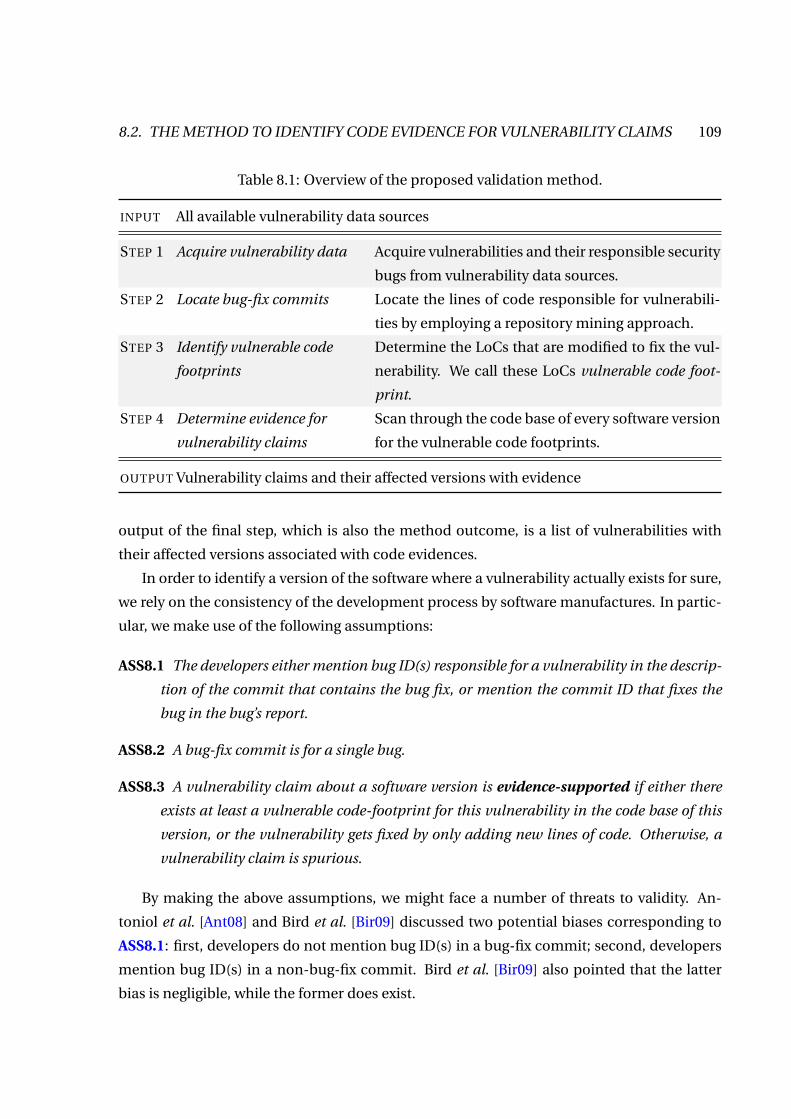
8.2. THE METHOD TO IDENTIFY CODE EVIDENCE FOR VULNERABILITY CLAIMS 109
Table 8.1: Overview of the proposed validation method.
INPUT All available vulnerability data sources
STEP 1 Acquire vulnerability data Acquire vulnerabilities and their responsible security
bugs from vulnerability data sources.
STEP 2 Locate bug-fix commits Locate the lines of code responsible for vulnerabili-
ties by employing a repository mining approach.
STEP 3 Identify vulnerable code
footprints
Determine the LoCs that are modified to fix the vul-
nerability. We call these LoCs vulnerable code foot-
print.
STEP 4 Determine evidence for
vulnerability claims
Scan through the code base of every software version
for the vulnerable code footprints.
OUTPUT Vulnerability claims and their affected versions with evidence
output of the final step, which is also the method outcome, is a list of vulnerabilities with
their affected versions associated with code evidences.
In order to identify a version of the software where a vulnerability actually exists for sure,
we rely on the consistency of the development process by software manufactures. In partic-
ular, we make use of the following assumptions:
ASS8.1 The developers either mention bug ID(s) responsible for a vulnerability in the descrip-
tion of the commit that contains the bug fix, or mention the commit ID that fixes the
bug in the bug’s report.
ASS8.2 A bug-fix commit is for a single bug.
ASS8.3 A vulnerability claim about a software version is evidence-supported if either there
exists at least a vulnerable code-footprint for this vulnerability in the code base of this
version, or the vulnerability gets fixed by only adding new lines of code. Otherwise, a
vulnerability claim is spurious.
By making the above assumptions, we might face a number of threats to validity. An-
toniol et al. [Ant08] and Bird et al. [Bir09] discussed two potential biases corresponding to
ASS8.1: first, developers do not mention bug ID(s) in a bug-fix commit; second, developers
mention bug ID(s) in a non-bug-fix commit. Bird et al. [Bir09] also pointed that the latter
bias is negligible, while the former does exist.
110 CHAPTER 8. A METHOD TO ASSESS VULNERABILITIES RETRO PERSISTENCE
The second assumption ASS8.2 is important because if a bug-fix commit contains changes
for fixing multiple bugs (i.e., multiple-bug-fix commit), we cannot distinguish the lines of
code (LoCs) that were touched to fix which bugs. Consequently we might end up with a re-
sult that vulnerability claims corresponding to these bugs are valid in the same versions of
software, which is not necessary true. Therefore if the number of multiple-bug-fix commit is
too high, this will rise threat biasing the outcome of the proposed method.
Concern ASS8.3, it is not necessarily true that the changed LoCs are the vulnerable ones,
albeit they might have helped to remove the vulnerability. For example, a vulnerability that
could lead to SQL injection attack could be fixed by inserting a sanitizer around a user’s input
in another module. We will then consider all versions where this sanitiser is missing as vul-
nerable. This is not necessary true; for example previous versions might have used another
model for input and the latter model had proper input sanitizer. This is acceptable in this
context because we are trying to minimize false negatives, while accepting false positives.
Occasionally we could not find evidence neither in favor nor against a vulnerability claim.
This could happen because either the corresponding CVE does not have any responsible se-
curity bug due to the incompleteness of the data source, or the bug-fix commit of the re-
sponsible bug cannot be located due to the incompleteness of the method.
Hereafter, we elaborate the steps of the proposed method.
8.2.1 Step 1: Acquire Vulnerability Data
For validation purposes, we need to obtain security bugs responsible for CVEs, from which
we can establish traces from CVEs to the code base. A CVE entry provides a general descrip-
tion of a vulnerability. Such description usually contains less technical information, and
emphasize more about the impact of a vulnerability so that it could be understandable by
most users. A security bug, in the other side, provides a more technical data for software
developer to fix the bug.
There are two official ways to obtain corresponding security bugs of a CVE. First, each
CVE might have references to its corresponding security bugs. These references are reported
in the references feature of a CVE. Second, the official security advisories by software manu-
facture might report CVE and its corresponding security bugs.
Example 8.1 Figure 8.2(a) shows an example where the corresponding security bug of CVE-
2008-5015 is reported as in its references feature. In this example, it is a URL to a security bug
report 447579 of Firefox. For Firefox, bug report hyperlinks usually have two forms: https:

8.2. THE METHOD TO IDENTIFY CODE EVIDENCE FOR VULNERABILITY CLAIMS 111
(a) Report detail for CVE-2008-5015 (b) Report detail for MFSA-2008-51
Figure 8.2: Selected features from a CVE (a), and from an MFSA report (b).
//bugzilla.mozilla.org/show_bug.cgi?id=n (for single bug), or https://bugzilla.
mozilla.org/bug_list.cgi?=n,n (for bug list). For Chrome, the hyperlink to a bug report
is usually http://code.google.com/p/chromium/issues/detail?id=n. In these hyper-
links, n is an integer number indicating the bug ID.
Example 8.2 Figure 8.2(b) illustrates an example where CVE and its corresponding secu-
rity bug are reported by vendor advisory reports, e.g., MFSA for Firefox. The figure shows a
snapshot of an MFSA entry: MFSA-2008-51. The References section of this entry reports two
hyperlinks: one for a security bug (https://bugzilla.mozilla.org/show_bug.cgi?id=
447579), and another one for a CVE entry (CVE-2008-5015). So we heuristically assume that
this security bug is responsible for that CVE.
8.2.2 Step 2: Locate Bug-Fix Commits
This step takes the list of vulnerabilities and their corresponding security bug identifier de-
termined in the previous step to locate their corresponding bug-fix commits in the code
base. A bug-fix commit is a commit entry in the code base repository that contains changes
to fix a (security) bug. There are two popular techniques to locate bug-fix commits: reposi-
tory mining and bug-report mining.

112 CHAPTER 8. A METHOD TO ASSESS VULNERABILITIES RETRO PERSISTENCE
Figure 8.3: Bug-fix commits
of Chrome (a) and Firefox
(b).
In each commit, the commit ID (i.e.,
revision ID), changed files, and fixed
bug ID are highlighted.
r41106 | [email protected] | 2010-03-10 02:03:43 +0100
(Wed, 10 Mar 2010) | 10 lines
Changed paths:
M /branches/249/src/chrome/browser/views/login_view.cc
Merge 40708 - This patch fixes [… text truncated for saving space]
BUG=36772
TEST=Try a hostname url longer than 42 chars to see that
it wraps correctly and wraps to the next line.
(a) A Chrome bug-fix commit
changeset: 127761:88cee54b26e0
author: Justin Lebar <[email protected]>
date: 2013-01-07 09:44 +0100
files: +|-|*dom/ipc/ProcessPriorityManager.cpp
desc: Bug 827217 - Fix null-pointer crash with webgl.can-
lose-context-in-foreground=false.
(b) A Firefox bug-fix commit
• The repository mining technique was introduced by Sliwerski et al. [Sli05] and adopted
by many other studies in the literature e.g., [Neu07; Shi11]. This technique parses com-
mit logs of the code base repository for the security bug IDs according to predefined
patterns. In our case, the commit logs mentioning security bug ID(s) are bug-fix com-
mits.
• The bug-report mining technique, adopted by Chowdhury and Zulkernine [CZ11], parses
a security bug report for bug-fix information. Such information includes changed lo-
cations in code base, which could be referred to as either links to bug-fix commits, or
links to particular revision of changed source files. In the latter case, we assume the
revision of changed source files is bug-fix commit.
Example 8.3 In Chrome, a bug-fix commit refers to bug IDs by the patterns BUG=n(,n)
or BUG=http://crbug.com/n, where n is the bug ID. In Firefox, bug IDs usually follow key-
words such as bug. Figure 8.3 exemplifies two bug-fix commits: one for Chrome, and another
one for Firefox. In each bug-fix commit, we highlight interesting information including the
revision ID of the bug-fix commit, the list of changed source files, and the bug ID fixed by the
commit.
These two techniques are complement each other since the advantage of a technique is
the disadvantage of the other. The repository mining technique requires access to commit
8.2. THE METHOD TO IDENTIFY CODE EVIDENCE FOR VULNERABILITY CLAIMS 113
logs which might not be publicly available. It could locate bug-fixes for undisclosed bug
reports – the advantage. However it might skip bug-fixes which do not mention explicitly
the security bug IDs (e.g., when merging from external repositories) – the disadvantage. On
the other hand, the bug-report mining technique could parse the bug report the bug-fixes
even if the bug IDs were not mentioned in these bug-fixes – the advantage. But it could not
locate bug-fixes for undisclosed bug reports, though these bug-fixes explicitly mention the
bug IDs – the disadvantage.
Example 8.4 For instance, bug-fixes for the WebKit module3 in Chrome usually do not con-
tain the bug IDs because they are merged from another repository.
With reference to ASS8.2, after identifying bug-fixes we should investigate the distri-
bution of number of bugs fixed per bug-fix commit to understand the potential impact of
multiple-bug-fix commits.
8.2.3 Step 3: Identify Vulnerable Code Footprints
This step takes bug-fix commits and annotates source files in the commits to determine vul-
nerable code footprints. A vulnerable code footprint is a piece of code which is changed (or
removed) in order to fix a security bug. The intuition to identify such vulnerable code foot-
prints is to compare the revision where a security bug is fixed (i.e., bug-fix commit) to its
immediate parent revision. Pieces of code that appear in the parent revision but not in the
bug-fixed revision are considered vulnerable code footprints.
Let r f i x be the revision ID of a bug-fix commit. We compare every file f changed in
this revision to its immediate parent revision4. We employ the diff command supported
by the repository to do the comparison. By parsing the comparison output, we can identify
the vulnerable code footprints. We ignore formatting changes such as empty lines, or lines
which contain only punctuation marks. Such changes occur frequently in all source files,
and therefore they do not characterize the changes to fix security bugs.
Example 8.5 Figure 8.4(a) illustrates an excerpt of the comparison between revision r 95730
and r 95731 of file url_fixer_upper.cc by using diff command. The command produces
3The module used by Chrome to render HTML pages4In an SVN repository, the immediate parent of the revision r f i x is r f i x −1. In some other repository such
as Mercurial, the immediate parent is determined by performing the command parent

114 CHAPTER 8. A METHOD TO ASSESS VULNERABILITIES RETRO PERSISTENCE
Figure 8.4: Excerpts of the
output of diff (a), and of
the output of annotate (b).
$ svn diff -r 95730 -r 95731 url_fixer_upper.cc
@@ -540,3 +540,6 @@
bool is_file = true;
+ GURL gurl(trimmed);
+ if (gurl.is_valid() && ...)
+ is_file = false;
FilePath full_path;
- if (!ValidPathForFile(...)
+ if (is_file && !ValidPathForFile(...)
start line index and number of lines of the left, and the right revisions
added line is preceded by a ‘+’
deleted line is preceded by a ‘-’
left revision right revision
(a) An excerpt of diff
$ svn annotate -r 95730 url_fixer_upper.cc
...
537: 15 initial.commit PrepareStringForFile...
538: 15 initial.commit
539: 15 initial.commit bool is_file = true;
541: 8536 [email protected] FilePath full_path;
542: 15 initial.commit if (!ValidPathForFile(...))
543: 15 initial.commit // Not a path as entered,
...
committed revision committer line contentline index
(b) An excerpt of annotate
an output in Unify Diff format where changes are organized in hunks. A hunk begins with
a header which is surrounded by double-at signs (@@), contains the start line index and
number of lines. Added lines, deleted lines, and unchanged lines are respectively preceded
by a plus sign, a minus sign, and a space character. The vulnerable code footprint is deleted
lines e.g., in this excerpt, which is line #542.
Next, we identify the origin of vulnerable code footprints i.e., the revision where the po-
tential bad code is introduced. Such origins are achieved by annotating the source file f at
immediate parent revision of the bug-fix commit. In an annotation of a source file, every in-
dividual line is annotated with meta-information such as the origin revision, the committed
time, and the author. The annotation is done by the annotate command of the repository
Example 8.6 Figure 8.4(b) presents an excerpt of the annotation of file url_fixer_upper.
cc at the immediate parent revision of the bug-fix commit, i.e., revision 95730. According to
this excerpt, the origin revision of vulnerable code footprint #542 in Example 8.5 is 15.

8.2. THE METHOD TO IDENTIFY CODE EVIDENCE FOR VULNERABILITY CLAIMS 115
Table 8.2: The execution of the method on few Chrome vulnerabilities.
CVE Reported
Versions
Bug ID Bug-fix Commits Footprint Versions w/
Evidence
2011-2822 v1–v13 72492 url_fixer_upper.cc1
(r 95731)
⟨r 15,542⟩ v1–v13
2011-4080 v1–v8 68115 media_bench.cc2
(r 70413)
⟨r 26072,352⟩,⟨r 53193,353⟩
v3–v8
2012-1521 v1–v18 117110 – – –
1: chrome/browser/net/url_fixer_upper.cc 2: media/tools/media_bench/media_bench.cc
8.2.4 Step 4: Determine Vulnerability Evidences
This step scans through the code base of all version claimed to be vulnerable for the existence
of vulnerable code footprints. Such existence is the supported evidence for the claimed that
a version is actually vulnerable to a vulnerability. A special case is present when a CVE was
fixed by only adding new code. In this case, no vulnerable code footprint is detected. In this
scenario, we assume conservatively that all original LoCs of the file where a vulnerability is
fixed are all vulnerable code footprints. If a version contains the file, then it is vulnerable.
This solution does not introduce false negatives, but may let false positives survive. Indeed
notice that the version has been already claimed to be vulnerable. For a compliance per-
spective, this is acceptable albeit maybe costly.
Example 8.7 Table 8.2 shows a few validation examples of Chrome vulnerability claims.
CVE-2011-2822 is reported to affect Chrome v1 up to v13. Its responsible bug is 72492. In
Step 2, by scanning the log, the bug-fix commit is revision r 95731 of file url_fixer_upper.
cc. In Step 3, we diff revision r 95730 and r 95731 of this file (see Figure 8.4(a)). The vulnerable
code footprint is determined as #542. Then we annotate r 95730 of the file to get the revision
of the code footprint, which is r 15 (see Figure 8.4(b)). In Step 4, we scan for this line in the
code base of all versions, and found it in v1 to v13. Finally, we identify the vulnerable versions
for this vulnerability, which are v1–v13.
Example 8.8 This example illustrates a case where the rule “version X and its previous ver-
sions are vulnerable” was applied. The description CVE-2012-4185 said:
“Buffer overflow in the nsCharTraits::length function in Mozilla Firefox before
16.0, Firefox ESR 10.x before 10.0.8, Thunderbird before 16.0, Thunderbird ESR

116 CHAPTER 8. A METHOD TO ASSESS VULNERABILITIES RETRO PERSISTENCE
10.x before 10.0.8, and SeaMonkey before 2.13 allows remote attackers to execute
arbitrary code or cause a denial of service (heap memory corruption) via unspeci-
fied vectors.”
By applying the above strategy, all versions from v1.0 – v15.0 are claimed as vulnerable to
this vulnerabilities. The corresponding bug for this CVE is 785753. This bug indicated that
it was a global-buffer-overflow in the nsCharTraits::length function. This bug was fixed
by changing the file netwerk/base/src/nsUnicharStreamLoader.cpp as follows.
if (NS_FAILED(rv))
- NS_ASSERTION(0 < capacity - haveRead,
- "Decoder returned an error but filled the output buffer! "
- "Should not happen.");
+ if (haveRead >= capacity)
+ // Make room for writing the 0xFFFD below (bug 785753).
+ if (!self->mBuffer.SetCapacity(haveRead + 1, fallible_t()))
+ return NS_ERROR_OUT_OF_MEMORY;
+
+
self->mBuffer.BeginWriting()[haveRead++] = 0xFFFD;
++consumed;
The plus (+) determines newly added lines, and the minus (-) indicates deleted lines. In this
case, the vulnerability’s cause might be the lack of a conditional check for a circumstance
that the Firefox developers did not think it would happen. It was fixed by adding the missing
check. We traced the original revision of the deleted line and found that it was introduced
since the revision 70061, and stayed there until revision 108991. We scanned through the
code based of Firefox v15 and downward for deleted lines. We could only found these deleted
lines in Firefox v6 to v15. Clearly, we could not say this vulnerability affects also Firefox v1.0
to v5.0 as claimed by this NVD entry.
8.3 Related Work
Sliwerski et al. [Sli05] proposed a technique that automatically locates fix-inducing changes.
This technique first locates changes for bug fixes in the commit log, then determines ear-
lier changes at these locations. These earlier changes are considered as the cause of the
later fixes, and are called fix-inducing. This technique has been employed in several studies

8.4. CHAPTER SUMMARY 117
[Sli05; Zim07] to construct bug-fix data sets. However, none of these studies mention how
to address bug fixes which earlier changes could not be determined. These bug fixes were
ignored and became a source of bias in their work.
Bird et al. [Bir09] conducted a study the level bias of techniques to locate bug fixes in code
base. The authors have gathered a data set linking bugs and fixes in code base for five open
source projects, and manual checked for the biases in their data set. They have found strong
evidence of systematic bias in bug-fixes in their data set. Such bias might be also existed
in other bug-fix data set, and could be a critical problem to any study relied on such biased
data.
Antoniol et al. [Ant08] showed another kind of bias that the bug-fixes data set might suffer
from. Many issues reported in many tracking system are not actual bug reports, but feature
or improvement requests. Therefore, this might lead to inaccurate bug counts. However,
such bias rarely happens for security bug reports. Furthermore, Nguyen et al. [Ngu10], in
an empirical study about bug-fix data sets, showed that the bias in linking bugs and fixes
is the symptom of the software development process, not the issue of the used technique.
Additionally, the linking bias has a stronger effect than the bug-report-is-not-a-bug bias.
Meneely et al. [Men13] studied the properties of so-called vulnerability-contributing com-
mits (VCC) which are similar to the commits containing vulnerability code footprints in this
chapter. Meneely et al. applied the similar method to identify security bug-fix commits, but
then they follow an ad-hoc approach to identify VCC. Thus, the identification of VCC for 68
vulnerabilities of Apache HTTP server took them hundreds of man-hours over six months.
Here, we have to deal with thousands of vulnerabilities.
8.4 Chapter Summary
This chapter presented a method to identify code evidence for vulnerability claims. The
method was inspired by the work of Sliwerski et al. [Sli05]. Sliwerski et al. [Sli05] aimed to
identify to code inducing fixes for bugs in general, meanwhile the proposed method focused
on the evidence of the present of vulnerabilities. Such objectives resulted in the significant
difference between the two methods: the method by Sliwerski et al. [Sli05] tried to reduce
false positives, while the proposed method aimed to reduce false negatives, and could accept
false positives.
The method took a list of vulnerabilities and their corresponding security bugs as input.
Then it traced the commits in the source code repository for the commits that fixed security
bugs. From these commits, it determined the so-called vulnerable code footprints which are

118 CHAPTER 8. A METHOD TO ASSESS VULNERABILITIES RETRO PERSISTENCE
changed LoCs to fix security bugs. Then it traced for the origin revision where vulnerable
code footprints were introduced. Finally it scanned the code base of individual versions to
determine the vulnerable status of these versions.
In the next chapter, we are going to check the effectiveness of the proposed method in the
sense that whether it can assess the vulnerabilities claims by NVD for Chrome and Firefox.
We also conduct experiments to see whether there is any bias in NVD vulnerability claims,
and how the potential bias might impact the conclusion of scientific studies relying on them.

CH
AP
TE
R
9AN EMPIRICAL ASSESSMENT FOR THE
RETRO PERSISTENCE OF VULNERABILITY
CLAIMS BY NVDThis chapter applies the assessment method for the retro persistence of vulnerabili-
ties described in Chapter 8 to empirically assess the vulnerability claims by NVD for 33
major versions of Chrome and Firefox. We used the proposed method to validate the
folk knowledge that when inserting data in NVD, analysts apply overly a conserva-
tive rule “version X and its previous versions are vulnerable”. The experiment results
have shown that more than 30% of vulnerability claims to each of these versions are
spurious. As a result, many scientific studies claiming that vulnerabilities tend to be
foundational were not in reality due to the NVD marking scheme.
WE in this chapter present an experiment to study whether the proposed assess-
ment method for the retro persistence of vulnerabilities actually works or not.
The experiment analyzes vulnerability claims by NVD for 33 major versions of
Chrome and Firefox. We aim to validate the folk knowledge that when making vulnerability
claims for each NVD entry, the NVD analysts apply overly a conservative rule “version X and
its previous versions are vulnerable.".
The rest of this chapter is organized as follows. Section 9.1 describes the chapter’s re-
search questions. Section 9.2 shows the analysis on the collected data for Chrome and Fire-
119

120 CHAPTER 9. THE ASSESSMENT OF THE NVD VULNERABILITY CLAIMS
fox. Section 9.3 reviews the impact of spurious vulnerability claims to two vulnerability stud-
ies. Section 9.4 presents potential threats to validity and how they are addressed. Section 9.5
summarizes this chapter.
9.1 Research Questions
In this chapter, we consider the following research questions:
RQ8 Is the proposed assessment method effective in assessing the retro persistence of vulnera-
bilities?
RQ9 To what extend are vulnerability claims by NVD trustworthy?
RQ10 To what extend does the bias in vulnerability claims by NVD (if any) impact conclusions
of a vulnerability analysis?
To study the effectiveness of the proposed assessment method i.e., answering RQ8, we
apply the proposed method to conduct an experiment assessing the number of spurious
vulnerability claims for 18 major versions of Chrome (i.e., v1.0–v18), and 15 major versions
of Firefox ( i.e., v1.0–v12.0). We measure the ability to assess the majority of vulnerability
claims of Chrome and Firefox. If the method could be able to assess at least two third of
vulnerability claims, it will be an evidence for the effectiveness of the proposed method.
We answer RQ9 by measuring the ratio of spurious vulnerability claims, which is here-
after referred to as error rate. In many analyses, a small error rate could be acceptable, but
other analyses might be biased. Suppose that we have two vulnerability samples X and Y
(for example, foundational vulnerabilities in Chrome and Firefox), we want to test whether
the outputs of a function f (e.g., mean, rank, standard error, or so) on X and Y are signif-
icantly different. The statistical test is basically a diff function measuring the chance that
f (X ) is different from f (Y ). Traditionally the significance level is 0.05 which means that if
diff ( f (X ), f (Y )) is greater than 0.95, we could conclude a significant difference. However, if
X contains more than 5% of errors, we are measuring diff ( f (X −0.05), f (Y )). If the errors are
not uniformly distributed, the errors might impact the output of f . Consequently, the eval-
uation of true diff might have passed from lower than 5% to greater than 5%. As the result,
the conclusion might not be statistically significant. From an industry perspective a greater
error rate that might introduces a notion of reasonable doubt to a compliance assessment.
We further examine the systematic characteristic of the spurious vulnerability claims
along the life time of each version – version age (i.e., the number of months since the release

9.2. THE ASSESSING EXPERIMENT OF VULNERABILITY CLAIMS 121
of particular versions). Industry-wise the presence of a systematic bias might lead to system-
atic deployment of over restrictive security measures or to the unwarranted preference of a
software over another.
We conduct another experiment to address RQ10. The experiment explores the effect of
spurious vulnerability claims to the validity of the studies on foundational vulnerabilities in
order to revisit the finding that the majority of vulnerabilities are foundational[OS06]. We
analyze the difference in the conclusions made in two different settings. The first setting
uses all vulnerabilities claimed by NVD. The second setting also uses vulnerabilities claimed
by NVD, but excludes all spurious ones.
9.2 The Assessing Experiment of Vulnerability Claims
We apply the proposed method to validate the trustworthiness of vulnerability claims by
NVD on Chrome and Firefox (answer for RQ9). For Firefox we obtain bug-fix commits by
using the repository mining technique because it discovered bug-fix commits for almost se-
curity bugs. For Chrome, we also use the repository mining technique for undisclosed secu-
rity bugs reports, and the bug-report mining technique for security bugs fixed in imported
projects (e.g., WebKit). These security bugs, as discussed, cannot be located by mining the
repository because their bug IDs were not mentioned in the bug-fix commits.
The implementation scripts of the method take approximately 14 days (i.e., 336 hours) on
a 2 x quad-core 2.83GHz Linux machine with 4GB of RAM to assess approximately 9,800 vul-
nerability claims for Chrome and Firefox. However it is still dramatically more efficient than
an ad-hoc approach adopted by Meneely et al. [Men13], which took six months to evaluate
68 vulnerabilities.
Hereafter, we present the software infrastructure for the experiment, and some statistics
of the experiment, as well as our analysis on the spurious vulnerability claims for these two
browsers.
9.2.1 The Software Infrastructure
Figure 9.1 presents the software infrastructure for the experiment that assesses the retro per-
sistence of Chrome and Firefox vulnerabilities. The body of this infrastructure consists of the
following scripts:
• Commit Log Parser. This script takes the commit logs of the source code repositories of
browsers, and vulnerability data of Chrome and Firefox (i.e., Chrome VDB and Firefox

122 CHAPTER 9. THE ASSESSMENT OF THE NVD VULNERABILITY CLAIMS
Firefox CVS
Repository
Firefox HG
Repository
Chrome SVN
Repository
Firefox CVS
Commit Logs
Firefox HG
Commit Logs
Chrome SVN
Commit Logs
Commit Log
Parser
CVS Log Parser
HG Log Parser
HG Log Parser
Code Tracer
BugFixes
CVS Wraper
HG Wraper
HG Wrapper
Repository Utility
Code
Footprints
Code Scanner
Firefox VDB
Chrome VDB
Bug
Verification
Data
Data Synthesizer
Firefox Verified VDB
Chrome Verified VDB
Retro Persistence
Analysis
Foundational Vulnerability
Analysis
Quarterly Trend Analysis
for Foundational
Vulnerability
Sphinx
scripts
R
scripts
Intermediate
Data
Output Dataset
Control Flow
DataFlow
Figure 9.1: The software infrastructure for assessing the vulnerabilities retro persistence.
VDB, see Section 4.1) as inputs to produce the BugFixes data set. Because the reposi-
tory of Firefox was migrated from CVS to HG since version v3.5, we have three different
kinds of commit logs: Firefox CVS Commit Logs, Firefox HG Commit Logs, Chrome SVN
Commit Logs. These commit logs are text files. Thus, this script relies on particular
parsing script for each type of commit logs (i.e., CVS Log Parser, HG Log Parser, and
SVN Log Parser). The BugFixes data set maintains the links between security bugs to
particular source components that were touch to fix it.
• Code Tracer. This script consumes the BugFixes data set to produce the Code Footprint
data set, which maintains the links between a security bug to particular LoCs that po-
tentially contribute to the existence of this bug. For this purpose, this script looks for
the original version of modified LoCs of source components in BugFixes. This is done
thank to the repository servers via the Repository Utility scripts.
• Code Scanner. This script scans LoCs in Code Footprint in the code bases of all versions
of Chrome and Firefox to determine the earliest version affected by a security bug. This
is also done with the aid of repository servers via the Repository Utility scripts. The
outcome of this script is the Bug Verification Data data set.

9.2. THE ASSESSING EXPERIMENT OF VULNERABILITY CLAIMS 123
• Data Synthesizer. This script aggregates data from Chrome and Firefox vulnerabilities
plus the Bug Verification Data data set to produce Firefox Verified VDB, and Chrome
Verified VDB data sets. These data sets are basically the same as Firefox VDB, and
Chrome VDB plus extra information about the earliest version affected by each vul-
nerability. The aggregated data sets are then consumed by analysis scripts to produce
desired outputs for answering research questions.
The schemas of the data sets mentioned in Figure 9.1 are as follows:
BugFixes = (bugID, browser, repository, xedCommit, component)
Code Footprint = (bugID, browser, repository, originalCommit, component, LoC)
Bug Verification Data = (bugID, browser, component, version, LoC)
Firefox Verified VDB = (bugID, bugDate, mfsaID, mfsaDate,
cveID, cveDate, minAectedVersion,
maxAectedVersion, estimatedMinVersion)
Chrome Verified VDB = (bugID, bugDate, cveID, cveDate,
minAectedVersion, maxAectedVersion, estimatedMinVersion)
9.2.2 Descriptive Statistics
Table 9.1 presents the numbers of CVEs affecting Chrome and Firefox by April 2013. Particu-
larly, there are 768 CVEs affecting Chrome, and 876 CVEs affecting Firefox. Out of those, 728
Chrome CVEs (94.8%), and 730 Firefox CVEs (83.3%) have at least one responsible security
bug. These CVEs make a total of 9,800 vulnerability claims to 18 major versions of Chrome
(v1–v18), and 15 major versions of Firefox (v1.0–v12.0).
The detailed outcomes of the experiment for vulnerability claims in individual versions
of Chrome and Firefox are reported in Table 9.2, Table 9.3, respectively. On average, each
version of Chrome has about 309 vulnerability claims. Of these, approximately 28.6% are
unverifiable, and 35.9% are found spurious by our method. The average number of vulnera-
Table 9.1: Descriptive statistics for vulnerabilities of Chrome and Firefox
Number of CVEs Total
verifiable w/o resp. bugs w/o bug-fix
Chrome 554 (72.1%) 40(5.2%) 174(22.7%) 768
Firefox 681 (77.7%) 146(16.7%) 49(5.6%) 876

124 CHAPTER 9. THE ASSESSMENT OF THE NVD VULNERABILITY CLAIMS
Table 9.2: Descriptive statistics of vulnerability claims of Chrome.
Unverifiable Verifiable
Release Total w/o resp. bug w/o bug-fix w/ evidence spurious
Chrome v1 526 5.9% 22.1% 34.8% 37.3%
Chrome v2 512 3.9% 22.7% 36.1% 37.3%
Chrome v3 504 3.6% 22.8% 38.7% 34.9%
Chrome v4 498 3.4% 22.5% 43.0% 31.1%
Chrome v5 455 1.1% 22.2% 38.9% 37.8%
Chrome v6 405 1.2% 24.0% 43.0% 31.9%
Chrome v7 391 1.3% 24.6% 42.2% 32.0%
Chrome v8 371 1.3% 24.5% 43.7% 30.5%
Chrome v9 337 1.5% 26.4% 42.7% 29.4%
Chrome v10 304 1.3% 28.0% 40.1% 30.6%
Chrome v11 273 1.8% 26.0% 38.1% 34.1%
Chrome v12 239 2.1% 25.5% 38.1% 34.3%
Chrome v13 217 1.8% 25.3% 36.9% 35.9%
Chrome v14 177 2.3% 22.6% 32.2% 42.9%
Chrome v15 121 4.1% 24.8% 38.0% 33.1%
Chrome v16 112 3.6% 25.0% 26.8% 44.6%
Chrome v17 88 4.5% 27.3% 20.5% 47.7%
Chrome v18 35 5.7% 48.6% 5.7% 40.0%
Mean(std.dev) 309 (155) 2.8% (1.5%) 25.8% (5.8%) 35.5% (9.3%) 35.9%(5.1%)
bility claims per each version of Firefox is slightly less than Chrome, about 283. Comparing
to Chrome, vulnerability claims per each Firefox version are less unverifiable (10.3%), and
slightly less spurious (31.5%).
As suggested in Step 2 (see Section 8.2.4), we investigate the distribution of fixed bugs
per bug-fix commit to understand the unwanted effect of multiple-bug-fix commits that po-
tentially biases the experiment outcomes. Figure 9.2 shows these distributions for Chrome
(left) and Firefox (right). In almost all cases for Chrome and in over 90% for Firefox, a bug-fix
commit only contain fixes for one bug. Clearly developers of both Chrome and Firefox are
really focused on fixing security bugs; they fix each security bug individually, and commit the
bug-fix to the repository when a bug is fixed. This consistent behavior makes the unwanted

9.2. THE ASSESSING EXPERIMENT OF VULNERABILITY CLAIMS 125
Table 9.3: Descriptive statistics of vulnerability claims of Firefox.
Unverifiable Verifiable
Release Total w/o resp. bug w/o bug-fix w/ evidence spurious
Firefox v1.0 454 12.3% 6.2% 32.6% 48.9%
Firefox v1.5 461 12.6% 6.3% 38.8% 42.3%
Firefox v2.0 469 7.0% 5.5% 45.6% 41.8%
Firefox v3.0 388 4.6% 6.4% 45.1% 43.8%
Firefox v3.5 336 3.0% 6.5% 53.0% 37.5%
Firefox v3.6 310 2.9% 7.4% 52.3% 37.4%
Firefox v4.0 253 0.8% 8.3% 62.8% 28.1%
Firefox v5.0 230 0.0% 8.3% 67.4% 24.3%
Firefox v6.0 220 0.0% 7.7% 68.2% 24.1%
Firefox v7.0 210 0.0% 7.6% 68.1% 24.3%
Firefox v8.0 203 0.5% 7.9% 66.5% 25.1%
Firefox v9.0 196 0.0% 7.7% 66.8% 25.5%
Firefox v10.0 176 0.0% 8.0% 67.0% 25.0%
Firefox v11.0 175 0.0% 8.0% 70.3% 21.7%
Firefox v12.0 165 0.0% 8.5% 69.7% 21.8%
Mean(std.dev) 283 (108) 2.9% (4.3%) 7.4% (0.9%) 58.3% (12.2%) 31.4% (9.0%)
#Bugs per bug−fix commit
Den
sity
0.0
0.2
0.4
0.6
0.8
1.0 0.99
0.01 0.00 0.00
1 2 3 >3
(a) Chrome
#Bugs per bug−fix commit
Den
sity
0.0
0.2
0.4
0.6
0.8
1.0
0.91
0.050.02 0.02
1 2 3 >3
(b) Firefox
Figure 9.2: The number of bugs per bug-fix commit in Chrome (a) and in Firefox (b).
effect of multiple-bug-fix commit negligible in our experiment.
We further investigate the complexity of a security bug-fix commit in two aspects: the

126 CHAPTER 9. THE ASSESSMENT OF THE NVD VULNERABILITY CLAIMS
Components per bug−fix (Chrome)
Den
sity
0.0
0.1
0.2
0.3
0.4
0.5
0.6
0.7
0.38
0.20
0.120.07
0.04 0.03 0.02 0.01 0.02
0.11
1 2 3 4 5 6 7 8 9 10+
Components per bug−fix (Firefox)
Den
sity
0.0
0.1
0.2
0.3
0.4
0.5
0.6
0.7
0.63
0.130.08
0.04 0.02 0.02 0.01 0.01 0.010.04
1 2 3 4 5 6 7 8 9 10+
(a) Number of components per bug-fix commit
Vulnerable code footprints per bug (Chrome)
Den
sity
0.0
0.2
0.4
0.6
0.8
1.0
0.53
0.130.08
0.04 0.02 0.02 0.02 0.01 0.03
0.13
10 20 30 40 50 60 70 80 90 100+
Vulnerable code footprints per bug (Firefox)
Den
sity
0.0
0.2
0.4
0.6
0.8
1.0
0.38
0.150.10
0.06 0.03 0.04 0.03 0.03 0.02
0.18
10 20 30 40 50 60 70 80 90 100+
(b) Number of vulnerable code footprints per bug-fix commit
Figure 9.3: The complexity of bug-fix commits by number of source components (a) and by
number of vulnerable code footprints (b).
number of source components touched to fix a bug, and the number of vulnerable code foot
prints. The intuition behind this investigation is that a less complex bug-fix commit will
generate less bias in the experiment outcome.
Figure 9.3(a) reports the distributions of source components touched per bug-fix commit
for Chrome (left) and Firefox (right). In Chrome, 77% of the cases a security bug gets fixed
by touching at most four components, and 38% are fixed by touching only one component.
Meanwhile, in Firefox, 76% are fixed by touching at most two components, and up to 63% of
the cases are fixed by touching one component. Moreover, in terms of touched components,
the number of complicated security bugs which require touching over ten components is

9.2. THE ASSESSING EXPERIMENT OF VULNERABILITY CLAIMS 127
about 11% in Chrome, and only 4% in Firefox. In short, bug-fix commits touching one com-
ponent take the largest portion in both Chrome and Firefox. They are majority in Firefox, but
are not in Chrome nonetheless.
Figure 9.3(b) exhibits the histograms of vulnerable code footprints per bug-fix commit
for Chrome (left) and Firefox (right). In Chrome, 78% security bugs have up to 40 vulnerable
code footprints, of those 53% have up to 10 footprints. In Firefox, 76% security bugs have
up to 60 footprints, 10-footprint (or less) security bugs are only 38%. Here we can see an
opposite observation between Chrome and Firefox, 10-footprint security bugs are majority
in Chrome, but are not in Firefox, although they also take the largest portions in the distri-
butions of both Chrome and Firefox.
On average, for two-third of Chrome security bugs, each has 15.26 vulnerable code foot-
prints, and gets fixed by touching 1.84 components. Those numbers for Firefox are 21.18
and 1.17. Apparently, security bugs are local phenomena, which might help to reduce the
potential bias in the proposed method.
9.2.3 The Analysis on the Spurious Vulnerability Claims
Table 9.2 and Table 9.3 show a non-negligible amount of unverifiable vulnerability claims
for both Chrome and Firefox, approximately 28.6% and 10.3% respectively. The error rate
measured by the ratio of the spurious vulnerability claims to the total ones in each analyzed
version could be significantly worse. At best all, these unverifiable vulnerability claims are
not spurious. The measured error rate is therefore the lower bound of the actual value. In the
sequel, we define two error rates: optimistic error rate (OER) and pessimistic error rate (PER).
OER(v) = |spurious(v)||vulnerabilities(v)| (9.1)
PER(v) = |spurious(v)|+ |unverifiable(v)||vulnerabilities(v)| (9.2)
where v is a version; |spurious(v)|, |unverifiable(v)|, and |vulnerabilities(v)| are the number
of spurious, unverifiable, and total vulnerabilities of v .
From (9.2) and (9.1), it is clearly that the PER is always greater than the OER. Thus the
OER is the lower bound of the actual error rate. If the OER is bad, the actual error rate and
the PER are even worse.
We study the systematicness of the error rates. The study period covers first 36 months
of each version because the version life cycle (i.e., interval between two consecutive major
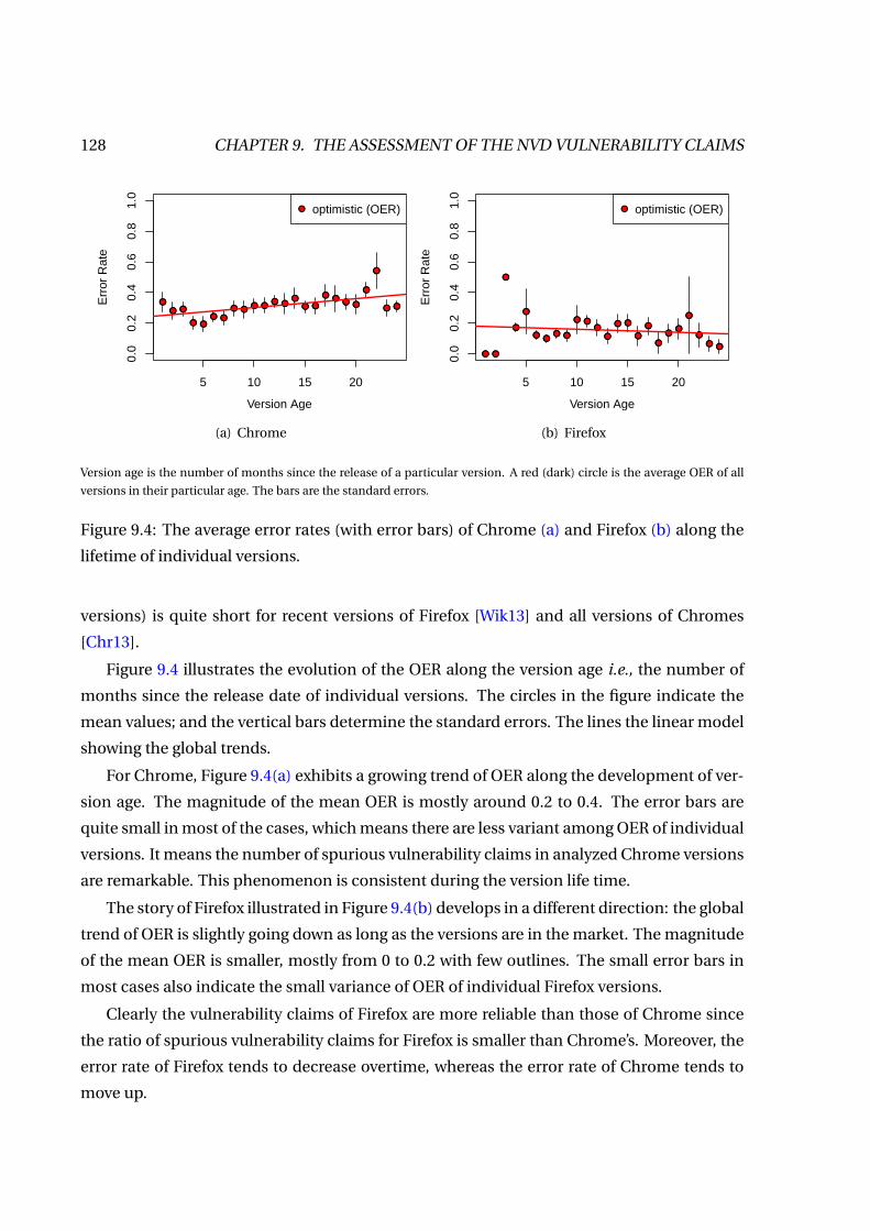
128 CHAPTER 9. THE ASSESSMENT OF THE NVD VULNERABILITY CLAIMS
5 10 15 20
0.0
0.2
0.4
0.6
0.8
1.0
Err
or R
ate
Version Age
optimistic (OER)
(a) Chrome
5 10 15 20
0.0
0.2
0.4
0.6
0.8
1.0
Err
or R
ate
Version Age
optimistic (OER)
(b) Firefox
Version age is the number of months since the release of a particular version. A red (dark) circle is the average OER of all
versions in their particular age. The bars are the standard errors.
Figure 9.4: The average error rates (with error bars) of Chrome (a) and Firefox (b) along the
lifetime of individual versions.
versions) is quite short for recent versions of Firefox [Wik13] and all versions of Chromes
[Chr13].
Figure 9.4 illustrates the evolution of the OER along the version age i.e., the number of
months since the release date of individual versions. The circles in the figure indicate the
mean values; and the vertical bars determine the standard errors. The lines the linear model
showing the global trends.
For Chrome, Figure 9.4(a) exhibits a growing trend of OER along the development of ver-
sion age. The magnitude of the mean OER is mostly around 0.2 to 0.4. The error bars are
quite small in most of the cases, which means there are less variant among OER of individual
versions. It means the number of spurious vulnerability claims in analyzed Chrome versions
are remarkable. This phenomenon is consistent during the version life time.
The story of Firefox illustrated in Figure 9.4(b) develops in a different direction: the global
trend of OER is slightly going down as long as the versions are in the market. The magnitude
of the mean OER is smaller, mostly from 0 to 0.2 with few outlines. The small error bars in
most cases also indicate the small variance of OER of individual Firefox versions.
Clearly the vulnerability claims of Firefox are more reliable than those of Chrome since
the ratio of spurious vulnerability claims for Firefox is smaller than Chrome’s. Moreover, the
error rate of Firefox tends to decrease overtime, whereas the error rate of Chrome tends to
move up.

9.3. THE IMPACT OF SPURIOUS VULNERABILITY CLAIMS 129
These inconsistent behaviors between two competing browsers could be potentially ex-
plained by the process that vulnerability claims are done. According to the private commu-
nication with NVD, the NVD analysis team do not perform any tests to determine which ver-
sions are affected by which CVEs. The vulnerability claims are derived from the CVE descrip-
tion by MITRE (www.mitre.org), release notes by software vendors, and additional data by
third-party security researchers. Therefore, to ensure completeness, all versions before a ver-
sion X are claimed vulnerable to a CVE if its description says something like: “version X and
before” or “X and ‘previous’ versions”. Apparently, in this case the NVD analysis team received
more detailed information for Firefox than for Chrome.
In summary, the experiment has provided evidences for the non-negligible error in the
vulnerability claims made by NVD to retrospective versions of Chrome and Firefox. This is
potentially the result of an unreliable process of making vulnerability claims. This evidence
therefore recommends a careful revision of scientific studies and, especially, any compliance
assessments that are relied upon such vulnerability claims.
9.3 The Impact of Spurious Vulnerability Claims
The previous analysis in Section 9.2.3 has shown a significant amount of spurious vulnera-
bility claims do exist. This section investigates the potential impact of spurious vulnerability
claims (RQ10) to scientific analyses based on such data. For this purpose, we examine two
studies about the majority of foundational vulnerabilities and the trend of foundational vul-
nerabilities.
9.3.1 The Majority of Foundational Vulnerabilities
A foundational vulnerability is a vulnerability which is introduced in the very first version
(i.e., v1.0), but continues to survive in next versions. In this section we revisit the claim on
the majority of foundational vulnerabilities: “Foundational vulnerabilities are the majority in
each version of both Chrome and Firefox". The claim could be formulated into the following
hypothesis.
H9.1A+ More than 50% of vulnerabilities of a version are foundational.
The subscript A+ indicates H9.1A+ is an alternative hypothesis. It means that if the re-
turned p-value of a statistic test is less than the significant level 0.05, we could reject the null
hypothesis and accept the alternative one.

130 CHAPTER 9. THE ASSESSMENT OF THE NVD VULNERABILITY CLAIMS
After a long evolution progress, modern versions of software might be completely dif-
ferent from the initial one. Obviously, foundational vulnerabilities should not be found in
these modern versions. Thus, the claim about the majority of foundational vulnerabilities
is eventually false. Therefore we relax the concept of foundation vulnerability to inherited
vulnerability, see also Section 5.2. An inherited vulnerability of a version X is a vulnerability
affecting X and its preceding versions. The claim about the majority of foundational vul-
nerabilities is relaxed to the claim about the majority of inherited vulnerabilities, which is
“Inherited vulnerabilities are the majority”. Similarly, we test the following hypothesis:
H9.2A+ More than 50% of vulnerabilities in a version X also exist in version X-1.
H9.3A+ More than 50% of vulnerabilities in a version X also exist in version Y which is older
than X at least 6 month.
The hypothesis H9.2A+ follows exactly the definition of inherited vulnerabilities. Mean-
while, the hypothesis H9.3A+ considers the short-cycle release policy where software ven-
dors try to ship a new version in a relative short period (e.g., less than 2 months per version).
Due to this policy, two consecutive versions might not have enough significant difference in
their code base. We assume that two versions which are different at least 6 month would
have significant changes in their code base.
We test these hypotheses in two data sets: one for all vulnerability claims by NVD, and
another one for vulnerability claims excluding ones which are found spurious by the pro-
posed method. To the brevity, we shortly refer to the former as NVD data set, and refer to the
latter as Verified NVD data set.
We could use either one-sided t-test or one-sided Wilcoxon signed-rank test. The former
tests on the mean, but requires the ratios to be normally distributed. The latter does not re-
quires normality, but tests on the median instead. Therefore, we first check the normality of
the ratios by the Saphiro-Wilk test. If the normality test returns p-value greater than 0.05, the
ratios are normally distributed. Then we will use t-test to check the hypothesis. Otherwise,
we will use Wilcoxon signed-rank test.
Figure 9.5 reports the distributions of foundational vulnerability claims for Chrome (a)
and Firefox (a), reported by both NVD (left) and Verified NVD (right) data sets. Clearly, in
these versions, foundational vulnerability claims are dominant, approximately 99% and 75%
per each version in Chrome and Firefox, respectively. The most remarkable difference be-
tween two data sets is that the amount of vulnerability claims (both foundational and non-
foundational) in the Verified NVD data set is dramatically lower than the NVD data set. This

9.3. THE IMPACT OF SPURIOUS VULNERABILITY CLAIMS 131
NVD(Chrome)
#vul
nera
bilit
ies
010
020
030
040
050
0
v2 (M
ay'09
)
v3 (S
ep'09
)
v4 (J
an'10
)
v5 (M
ay'10
)
v6 (S
ep'10
)
v7 (O
ct'10
)
v8 (D
ec'10
)
v9 (F
eb'11
)
v10
(Mar
'11)
v11
(Apr
'11)
v12
(Jun'1
1)
v13
(Aug
'11)
v14
(Sep
'11)
v15
(Oct'
11)
v16
(Dec
'11)
v17
(Feb
'12)
v18
(Mar
'12)
non−foundationalfoundational
NVD without spurious claims(Chrome)
#vul
nera
bilit
ies
010
020
030
040
050
0
v2 (M
ay'09
)
v3 (S
ep'09
)
v4 (J
an'10
)
v5 (M
ay'10
)
v6 (S
ep'10
)
v7 (O
ct'10
)
v8 (D
ec'10
)
v9 (F
eb'11
)
v10
(Mar
'11)
v11
(Apr
'11)
v12
(Jun'1
1)
v13
(Aug
'11)
v14
(Sep
'11)
v15
(Oct'
11)
v16
(Dec
'11)
v17
(Feb
'12)
v18
(Mar
'12)
spuriousnon−foundationalfoundational
(a) Chrome foundational vulnerabilities
NVD(Firefox)
#vul
nera
bilit
ies
010
020
030
040
050
0
v1.5
(Nov
'05)
v2.0
(Oct'
06)
v3.0
(Jun
'08)
v3.5
(Jun
'09)
v3.6
(Jan
'10)
v4.0
(Mar
'11)
v5.0
(Jun
'11)
v6.0
(Aug
'11)
v7.0
(Sep
'11)
v8.0
(Nov
'11)
v9.0
(Dec
'11)
v10.
0 (F
eb'12
)
v11.
0 (M
ar'12
)
v12.
0 (A
pr'12
)
non−foundationalfoundational
NVD without spurious claims(Firefox)
#vul
nera
bilit
ies
010
020
030
040
050
0
v1.5
(Nov
'05)
v2.0
(Oct'
06)
v3.0
(Jun
'08)
v3.5
(Jun
'09)
v3.6
(Jan
'10)
v4.0
(Mar
'11)
v5.0
(Jun
'11)
v6.0
(Aug
'11)
v7.0
(Sep
'11)
v8.0
(Nov
'11)
v9.0
(Dec
'11)
v10.
0 (F
eb'12
)
v11.
0 (M
ar'12
)
v12.
0 (A
pr'12
)
spuriousnon−foundationalfoundational
(b) Firefox foundational vulnerabilities
The dates in the X axis are the release dates.
Figure 9.5: Foundational vulnerabilities by NVD: all vulnerability claims (left) and spurious
vulnerability claims excluded (right).
is because of the high number of spurious vulnerability claims found in each version, see
Table ??. From the figure, foundational vulnerabilities are no longer dominant, especially for
Firefox v4.0 and onward.
Figure 9.6 reports the ratios of inherited vulnerabilities in individual versions of Chrome
and Firefox. In Figure 9.6(a), we count the inherited vulnerabilities of a version X from all
its preceded versions, see H9.2A+. Meanwhile, in Figure 9.6(b), we only count inherited vul-
nerabilities from preceded versions which are at least 6 month older, see H9.3A+. In this
figure, circles and squares denote the ratios of inherited vulnerabilities counted from NVD
and Verified NVD data sets, respectively.
From Figure 9.6 we can observed a similar phenomenon in the foundational vulnera-
bilities. In NVD data set, inherited vulnerabilities are dominant in both ways of counting.

132 CHAPTER 9. THE ASSESSMENT OF THE NVD VULNERABILITY CLAIMS
0.0
0.2
0.4
0.6
0.8
1.0
Inhe
rited
vul
nera
bilit
y ra
tio
v2 (M
ay'09
)
v3 (S
ep'09
)
v4 (J
an'10
)
v5 (M
ay'10
)
v6 (S
ep'10
)
v7 (O
ct'10
)
v8 (D
ec'10
)
v9 (F
eb'11
)
v10
(Mar
'11)
v11
(Apr
'11)
v12
(Jun'1
1)
v13
(Aug
'11)
v14
(Sep
'11)
v15
(Oct'
11)
v16
(Dec
'11)
v17
(Feb
'12)
v18
(Mar
'12)
NVDVerified NVD
Chrome
0.0
0.2
0.4
0.6
0.8
1.0
Inhe
rited
vul
nera
bilit
y ra
tio
v1.5
(Nov
'05)
v2.0
(Oct'
06)
v3.0
(Jun
'08)
v3.5
(Jun
'09)
v3.6
(Jan
'10)
v4.0
(Mar
'11)
v5.0
(Jun
'11)
v6.0
(Aug
'11)
v7.0
(Sep
'11)
v8.0
(Nov
'11)
v9.0
(Dec
'11)
v10.
0 (F
eb'12
)
v11.
0 (M
ar'12
)
v12.
0 (A
pr'12
)
NVDVerified NVD
Firefox
(a) Inherited vulnerabilities from preceded versions
0.0
0.2
0.4
0.6
0.8
1.0
Inhe
rited
vul
nera
bilit
y ra
tio
v2 (M
ay'09
)
v3 (S
ep'09
)
v4 (J
an'10
)
v5 (M
ay'10
)
v6 (S
ep'10
)
v7 (O
ct'10
)
v8 (D
ec'10
)
v9 (F
eb'11
)
v10
(Mar
'11)
v11
(Apr
'11)
v12
(Jun'1
1)
v13
(Aug
'11)
v14
(Sep
'11)
v15
(Oct'
11)
v16
(Dec
'11)
v17
(Feb
'12)
v18
(Mar
'12)
NVD(6)Verified NVD(6)
Chrome0.
00.
20.
40.
60.
81.
0
Inhe
rited
vul
nera
bilit
y ra
tio
v1.5
(Nov
'05)
v2.0
(Oct'
06)
v3.0
(Jun
'08)
v3.5
(Jun
'09)
v3.6
(Jan
'10)
v4.0
(Mar
'11)
v5.0
(Jun
'11)
v6.0
(Aug
'11)
v7.0
(Sep
'11)
v8.0
(Nov
'11)
v9.0
(Dec
'11)
v10.
0 (F
eb'12
)
v11.
0 (M
ar'12
)
v12.
0 (A
pr'12
)
NVD(6)Verified NVD(6)
Firefox
(b) Inherited vulnerabilities from preceded versions which are at least 6 month older
Figure 9.6: The ratios of inherited vulnerabilities in Chrome and Firefox.
However, they might be no longer dominant in Verified NVD data set. There is a weird data
point in Chrome’s: the number of inherited vulnerabilities in Figure 9.6(b) is 0. It is because
the interval between Chrome v1.0 and v2.0 was less than 6 months. By applying the counting
method described in H9.3A+, Chrome v2.0 does not have any inherited vulnerabilities.
We run the Shapiro-normality test on vulnerabilities data. Sometimes, it rejects the null
hypothesis (i.e., data is not normality, p-value = 0.07 · 10−6 – Chrome, NVD), sometime it
does not (i.e., data is normality, p-value = 0.95 – Firefox, NVD). Therefore, we use Wilcoxon
signed-rank test to check the hypotheses. The outcomes of the hypothesis tests are reported
in Table 9.4. Notice that the reported p-values are for rejecting the null hypothesis. Therefore,
if p-value < 0.05, we accept the alternative hypothesis, and reject it otherwise.
Table 9.4 shows that if we rely on the NVD data set, all the hypotheses are accepted with
strong evidences (i.e., p-values are almost zero). However, if we use the Verified NVD data
set, which is NVD data set excluded the spurious vulnerability claims, we obtain the opposite
conclusions in most cases. It is therefore an evidence for the significant impact of spurious

9.3. THE IMPACT OF SPURIOUS VULNERABILITY CLAIMS 133
Table 9.4: The Wilcoxon signed-rank test results for the majority of foundational and inher-
ited vulnerabilities.
Numbers in parentheses are p-values returned by the Wilcoxon signed-rank test for the corresponding hypothesis. If
p-value < 0.05, the null hypothesis is rejected, it means we accept the alternative hypothesis. Otherwise, we reject the
alternative hypothesis.
Hypothesis NVD Verified NVD
Chrome Firefox Chrome Firefox
H9.1A+ More than 50% of vulnerabilities of a ver-
sion are foundational
Accept(0.01 ·10−2)
Accept(0.06 ·10−3)
Reject(1.00)
Reject(1.00)
H9.2A+ More than 50% of vulnerabilities in a ver-
sion X also exist in version X-1
Accept(0.01 ·10−2)
Accept(0.05 ·10−2)
Accept(0.03)
Reject(0.16)
H9.3A+ More than 50% of vulnerabilities in a ver-
sion X also exist in version Y which is
older than X at least 6 month
Accept(0.01 ·10−1)
Accept(0.05 ·10−2)
Reject(0.85)
Reject(0.67)
vulnerability claims to the study on the majority of foundational/inherited vulnerabilities.
Many foundational/inherited vulnerabilities do not really exist. They are a phenomenon
which can be better explained by the policy “version X and previous versions are vulnerable"
as discussed above.
9.3.2 The Trend of Foundational Vulnerability Discovery
In this study, we replicate the experiment described by Ozment and Schechter [OS06] to
study the existence and direction of trend in the discovery of foundational vulnerabilities.
We employ Laplace test for trend [NIS12a, Chap. 8] which was also used in [OS06] to search
for a trend quarterly during the browser age.
The Laplace test computes the Laplace factor which compares the centroid of the ob-
served discovery times with the mid-point of the observation period. This factor approxi-
mates the standardized normal random variable (e.g., z-score). The following formula shows
how the Laplace factor z is computed.
z =
p12n
n∑i=1
(ti − T
2
)n ·T
(9.3)

134 CHAPTER 9. THE ASSESSMENT OF THE NVD VULNERABILITY CLAIMS
where n is the number of foundational vulnerabilities discovered within the observation pe-
riod T ; ti is the interval (e.g., in days) between the discovery time of the i -th vulnerability
and the beginning time of the observation period. The interpretation of the Laplace factor z
is as follows:
• z > 1.96: there is a significant upward trend in the period T with 95% confidence.
• z <−1.96: there is a significant downward trend in the period T with 95% confidence.
• −1.96 ≤ z ≤ 1.96: there is either an upward trend (z > 0) or a downward trend (z < 0) in
the data, but the trend is not significant. Statistically speaking, we conclude there is no
trend in the observation period.
When the Laplace test indicates a significant trend (either increasing or decreasing trend)
in a certain time period, we call it an event. In a certain period, an event could be detected in
both data sets, i.e., NVD and Verified NVD, by the Laplace test. Sometimes, an event could
only be detected in only one data set. We refer to the former as common event, and the latter
as inconsistent event.
We want to determine whether spurious vulnerability claims have a significant impact
on the trends of foundation vulnerability discovery. For this purpose, we first perform the
Laplace test for quarterly trends of foundational vulnerabilities discovery along the age of in-
dividual versions in two data sets: NVD and Verified NVD. Then, for each version, we count
the number of inconsistent events. If the numbers of inconsistent events in all versions are
significantly different from 0, we could conclude a significant impact of spurious vulnerabil-
ity claims on the foundational vulnerability trends. In other words, we test the following null
hypothesis:
H9.40 The mean of inconsistent events in all individual versions is not significantly different
from 0.
We run the experiment on versions of Chrome and Firefox. In the experiment, we mea-
sure the interval ti of the i -th vulnerability by the number of days. However the published
dates of NVD are a poor approximation for the discovery dates of vulnerabilities [Res05;
Ozm05]. It is because when the NVD security team receive the vulnerability reports, they
usually wait for software vendors to fix the vulnerabilities before announcing the NVD en-
tries. Therefore, we approximate the discovery dates of vulnerabilities by the dates when
the bug reports corresponding to vulnerabilities were filed. By doing so, we assume that if a

9.3. THE IMPACT OF SPURIOUS VULNERABILITY CLAIMS 135
010
3050
Actual trends
3 6 9 15 21 27 33
NVDVerified−NVD
#vul
nera
bilit
ies
clai
ms
Version Age
(a) Chrome v5
010
3050
Actual trends
3 6 9 15 21 27 33
NVDVerified−NVD
#vul
nera
bilit
ies
clai
ms
Version Age
(b) Firefox v3.0
NVD: all vulnerability claims (with spurious ones); Verified NVD: vulnerability claims without spurious ones.
Figure 9.7: The actual discovery trends of foundational vulnerabilities.
Table 9.5: Number of events (i.e., significant quarterly trends)
Inconsistent Event
Browser Common Event Only NVD Only Verified NVD Total
Chrome (v2–v18) 23 (61%) 5 (13%) 10 (26%) 38 (100%)
Firefox (v1.5–v12.0) 5 (18%) 22 (78%) 1 (4%) 28 (100%)
Total 28 (42%) 27 (41%) 11 (17%) 66 (100%)
vulnerability is discovered by a white-hat researcher, he/she will notify (direct or indirectly)
software vendors as soon as possible. Then a bug report will be filed. For vulnerabilities
discovered by black-hat, we have no glue about the actual discovery dates.
Figure 9.7 reports the actual trends of foundational vulnerabilities for both Chrome (v5),
exemplified in Figure 9.7(a), and Firefox (v3.0), exemplified Figure 9.7(b). In this figure, the
solid line presents the trend reported by NVD, and dashed line indicates trend reported by
Verified NVD. For Chrome, the NVD trend and Verified NVD trend have similar shape, but
different from the magnitude. Meanwhile, for Firefox, these trends are clearly different in
both shape and magnitude.
We run the Laplace test for quarterly trends of foundation vulnerabilities of Chrome and
Firefox. Figure 9.8 reports the Laplace factors for Chrome v5.0. The figure shows the different

136 CHAPTER 9. THE ASSESSMENT OF THE NVD VULNERABILITY CLAIMS−
10−
50
510
NVD
−2
2
3 6 9 15 21 27 33
Lapl
ace
Fact
or
Version Age
−10
−5
05
10
Verified NVD
−2
2
3 6 9 15 21 27 33
Lapl
ace
Fact
orVersion Age
Figure 9.8: The Laplace test for quarterly trends in Chrome v5 foundation vulnerabilities.
−10
−5
05
10
NVD
−2
2
3 6 9 15 21 27 33
Lapl
ace
Fact
or
Version Age
−10
−5
05
10
Verified NVD
−2
2
3 6 9 15 21 27 33
Lapl
ace
Fact
or
Version Age
Figure 9.9: The Laplace test for quarterly trends in Firefox v3.0 foundation vulnerabilities.
outcomes of Laplace test by including or excluding spurious vulnerability claims (i.e., NVD
and Verified NVD data sets, respectively). Before month 12th, NVD reports two significant
increasing trends; Verified NVD reports one extra significant increasing trend, which will be
missed if we look at NVD. In contrast, after month 12th, NVD reports other two significant
trends, which do not appear in Verified NVD.
The Laplace factors for Firefox is reported in Figure 9.9. This figure also remarks the
difference of the Laplace outcomes between NVD and Verified NVD. The former reports
a significant trend during the life time of Firefox v3.0. This trend however disappear in the
latter data set. The complete Laplace tests for quarterly trend for Chrome and Firefox could
be found in the Appendix A.1, Figure A.1–A.2.
Table 9.5 summarizes the number of events identified by the Laplace test. This table re-

9.3. THE IMPACT OF SPURIOUS VULNERABILITY CLAIMS 137
NVD Verified NVD Total
01
23
45
#Inc
onsi
sten
t eve
nts
(a) Chrome
NVD Verified NVD Total
01
23
45
#Inc
onsi
sten
t eve
nts
(b) Firefox
Figure 9.10: The distribution of inconsistent events in NVD and Verified NVD.
ports the total number of common events (the second column), the number of inconsistent
events including events observed only in NVD (the third column), and events observed only
in Verified NVD (the forth column) in all analyzed versions of Chrome and Firefox. The table
shows that for Chrome, there are a lot of common events between two data sets (26 events
– 59%). This could be explained by the similarity of shape between the actual trends for
Chrome in both data sets (see Figure 9.7(a)). However, we can still observed the difference
between to data sets by looking at the number of inconsistent events (18 inconsistent events
– 41%). This difference is sharpen in the case of Firefox, the number of common events
is small (7 events – 20%), while the numbers of inconsistent event is large (28 inconsistent
events – 80%).
The breakdown distributions of inconsistent events in individual versions of Chrome and
Firefox are illustrated in Figure 9.10. Interested readers are referred to Appendix A.1, Ta-
ble A.1–A.2 for absolute numbers of the distributions.
We additionally run statistic test to see whether the numbers of inconsistent events in
individual versions of Chrome and Firefox are different from zero, see H9.40. The Shapiro-
Wilk normality test rejects the null hypothesis for both Chrome (p-value = 0.005) and Firefox
(p-value = 0.006). It means these distributions are not normal. Thus we rely on Wilcoxon
singed-rank test to check H9.40. The outcome of the Wilcoxon test also rejects H9.40 for
both Chrome (p-value = 0.003) and Firefox (p-value = 0.001). This means that the numbers
of inconsistent events are significantly greater than 0. In other words, it is an evidence for the

138 CHAPTER 9. THE ASSESSMENT OF THE NVD VULNERABILITY CLAIMS
significant impact of spurious vulnerability claims on the analysis about the quarterly trends
of foundational vulnerability discovery.
9.4 Threats to Validity
Construct validity includes threats affecting the approach by means of which we collect and
verify vulnerabilities. Threats in this category come from the assumptions as follows.
Bias in vulnerability data set. We apply the software infrastructure described in Chap-
ter 4. Thus the study in this chapter has a number of validity threats described in Section 4.2.
We also apply the mitigation procedures in Section 4.2 to minimize the threats.
Biases in bug-fix commit data. As outlined previously, there are two potential biases on
bug-fix commit data [Bir09]: the developers do not mention the bug ID in a bug-fix com-
mit; and the developers mention a bug ID in a non-bug-fix commit. To evaluate the impact
of the latter bias, we performed a qualitative analysis on some bug-fix commits and found
that all are actually bug fixes. This confirms the finding in [Bir09] for this type of bias. As
for the former bias, we check the completeness of the bug-fix commits for vulnerabilities. As
discussed, about one fourth of vulnerabilities are unverifiable (see also Table 9.1). We op-
timistically assumed that these vulnerabilities are not spurious. Therefore, our conclusions
are the lower bound of the real errors.
Bias in the validation method. The method assumption ASS8.3 is apparently syntactical
and might not cover all the cases of bug fixes since it is extremely hard to automatically un-
derstand the root cause of vulnerabilities. Therefore, the method classifies a NVD-reported
vulnerability of a particular version as correct while it may be a false-positive. Again it only
makes our conclusion lower bound of the real error, thus it make our case stronger.
Bias in the method implementation. It is possible that the implementation of the vali-
dation method has some bugs, causing bias in the identification of vulnerability evidences.
To minimize such problem, we employ multi-round test-and-fix approach where we ran the
program on some vulnerabilities, then we manually checked the output, and fixed found
bugs. We repeated this until no bug was found. Finally, we randomly checked the output
again to ensure there was no mistake.
Internal validity concerns the causal relationship between the collected data and the con-
clusion. Our conclusions are based on statistical tests. These tests have their own assump-
tions which may be violated by the data. To reduce the risk we carefully analyzed the as-

9.5. CHAPTER SUMMARY 139
sumptions of the tests: for instance, we did not apply any tests with normality assumption
since the distribution of vulnerabilities is not normal.
External validity is the extent to which our conclusion could be generalized to other ap-
plications. We tested the proposed method on browser but we did not use in any way this
information. The method could be used and the experiment could be replicated on different
software.
9.5 Chapter Summary
This chapter described an experiment applying the assessment method described in Chap-
ter 8 to assess the retro persistence validity of vulnerability claims by NVD for Firefox and
Chrome. The experiment has assessed 1,235 out of 1,644 CVEs (∼ 75%) in 33 versions of
Chrome and Firefox. The assessment took approximately 14 days. It is an evidence that the
proposed method is not only effective (i.e., majority of vulnerabilities have been assessed),
but also efficient (i.e., in comparison with 6 months for 68 vulnerabilities by using an ad-hoc
method [Men13]).
The experiment results have pointed out that about 30% of vulnerabilities claims by NVD
for Chrome and Firefox are spurious. It is also an evidence for the overdose of the rule “ver-
sion X and its previous versions are vulnerable” while marking which versions are vulnerable
to which vulnerabilities. In other words, retro versions of Chrome and Firefox have less vul-
nerabilities than they were reported.
We further have conducted other experiments to see to what extend spurious vulnerabil-
ity claims impact scientific vulnerability studies. In these experiments, we have revisited the
observation about the majority of foundational vulnerabilities in Chapter 5. By eliminating
all spurious vulnerabilities, we found that foundational vulnerabilities are no longer the ma-
jority in security landscape of individual versions of Chrome and Firefox. We even relaxed
the constraint to see whether inherited vulnerabilities are the majority. Again, we found only
a weak evidence that it is the case, but probably it is due to the short-cycle release policy cur-
rently adopted by software vendors. In another experiment analyzing the quarterly trends of
foundational vulnerabilities by using Laplace test, we have also noticed a significant different
between the reported trends by using the data with and without the spurious vulnerability
claims. These experiments have presented evidences that spurious vulnerability claims did
significantly impact the outcomes of scientific vulnerability studies.

140 CHAPTER 9. THE ASSESSMENT OF THE NVD VULNERABILITY CLAIMS
In the next chapter, we are going to describe the observation on the correlation between
dependency metrics and the vulnerable status of source components.

CH
AP
TE
R
10CONCLUSION
This chapter summarizes the observations, findings, as well as invented artifacts
presented in previous chapters of the dissertation. Based on that, the chapter also
discusses future research directions that could be leveraged by the outcomes of this
dissertation.
FROM the objective of the dissertation is to independently and systematically validate
an empirical models concerning vulnerabilities, we have presented several observa-
tions and artifacts serving for the objectives. This chapter summarizes the key points
of such observations and artifacts (Section 10.1), and discusses potential future research
based on the results of this dissertation (Section 10.2).
10.1 Summary of Contributions
Inspiring by the following key observations in the literature: an inadequate amount of dis-
cussion about the quality of data source in empirical experiments on vulnerabilities, and
critical issues in the traditional validation methodology for VDMs, as well as the lack of in-
dependent evaluation for proposed VDMs, we have conducted several activities and exper-
iments aiming at filling the observed gaps. Here are the main contributions of the disserta-
tion.
141
142 CHAPTER 10. CONCLUSION
A systematic survey on the usage of vulnerability data sources. We have conducted a sur-
vey about empirical vulnerability studies in past eight years from 2005 to 2012. The survey
included 59 publications, which were referred to as primary studies, in international work-
shops, conferences/symposium, and journals. The survey focused on the usage of vulnera-
bility data sources in the past. Concretely, it addressed the following research questions:
RQ1 Which are the popular data sources for vulnerability studies?
RQ2 Which data sources and features are used for which studies?
To find out the answers, the survey has presented a qualitative analysis the data usage in
59 collected primary studies. The analysis showed that third-party data sources were pre-
ferred more than other data sources in conducting empirical vulnerability studies. Among
several data sources, NVD was the most popular one, which was used in approximately 62%
of primary studies across different research topics. Among features of data sources, Affected
Versions (VA) and Announced Date (TA) are the most frequently used features in the collected
primary studies.
An empirical methodology for the evaluation of the performance of VDMs. The observa-
tion on past studies in the field of VDM has pointed several critical biases in the traditional
methodology, which were widely adopted in the literature, to evaluate the performance of
VDMs. These biases included: vulnerability definition bias – which concerned the way vul-
nerability was understood and counted, multi-version software bias – which concerned the
consideration of all versions of evolving software as a single entity, acceptance threshold bias
– which concerned how VDMs were either accepted or rejected while fitting on a data set,
and overfitting bias – which concerned the way VDMs were used in predicting future vulner-
ability trends.
These biases have impacted the outcomes of past evaluation experiments. Hence, we
have worked out on an empirical methodology that took into consideration all above issues
to address the two fundamental research questions in the field:
RQ3 How to evaluate the performance of a VDM?
RQ4 How to compare between two or more VDMs?
The methodology proposed two quantitative metrics: temporal goodness-of-fit quality, and
predictability. The former indicates how well a VDM could fit existing vulnerability data.
The latter determines how well a VDM could predict the future trends of vulnerabilities. The

10.1. SUMMARY OF CONTRIBUTIONS 143
methodology included a sequence of fully-discussed steps, which consisted of criteria and
justification in each step, that took input exactly as same as the input of the traditional eval-
uation methodology to produce more informative and precise outputs than the traditional
methodology. Additionally, the proposed methodology enabled a statistic-powered com-
parison between VDMs, which are undoubtedly better than the traditional one. The effec-
tiveness of the proposed methodology has been evaluated in an evaluation experiments on
several versions of mainstream web browsers.
An evaluation and comparison on the empirical performance of existing VDMs. As an
effort to evaluate the effectiveness of the proposed methodology to evaluate VDM perfor-
mance, we have conducted an evaluation experiment on thirty versions of mainstream web
browsers: Chrome, Firefox, Internet Explorer, and Safari. The experiment considered eight
VDMs: AML, AT, LN, JW, LP, RE RQ, and YF. The experiment focused on the following research
questions:
RQ6 Is the proposed VDM evaluation methodology effective in evaluating VDMs?
RQ7 Among existing VDMs, which one is the best?
By effective we meant the methodology could be able to evaluate VDMs and produce desired
results. The experiment has showed that AT and RQ model should not be used due to their
consistently low quality along the browser lifetime. Other models might be adequate. In-
terestingly, for young versions of browsers (no more than 12 months since the release date)
the simplest model – the LN model – was the best in terms of quality and predictability. For
middle age browsers (12 – 36 months), the AML model became the winner.
An empirical method for the assessment of vulnerabilities retro persistence. We pro-
posed an empirical method to identify code evidence for vulnerability claims. By this method,
we aimed to answer the following research question:
RQ5 How to estimate the validity of a vulnerability claim to a retro version of software?
The proposed method took a list of vulnerabilities and their corresponding security bugs as
input. Then it traced the commits in the source code repository for the commits that fixed
security bugs. From these commits, it determined the so-called vulnerable code footprints
which are changed LoCs to fix security bugs. Then it traced for the origin revision where
vulnerable code footprints were introduced. Finally it scanned the code base of individual

144 CHAPTER 10. CONCLUSION
versions to determine the vulnerable status of these versions. The outcome of the proposed
method will provide a better insight about the security landscape of retro versions of soft-
ware.
An assessment on the bias of vulnerability claims by NVD for Chrome and Firefox. We
have conducted an experiment applying the assessment method described in Chapter 8.
The experiment assessed the retro persistence validity of vulnerability claims by NVD for
Firefox and Chrome. The purposes of the experiment are to answer the following research
questions:
RQ8 Is the proposed assessment method effective in assessing the retro persistence of vulnera-
bilities?
RQ9 To what extend are vulnerability claims by NVD trustworthy?
RQ10 To what extend does the bias in vulnerability claims by NVD (if any) impact conclusions
of a vulnerability analysis?
Similar to evaluation experiment for VDMs, by the word “effective”, we wanted to know whether
the proposed assessment method is able to assess the majority of vulnerabilities. The exper-
iment has assessed the retro persistence of more than 75% (1,235 out of 1,644 CVEs) vul-
nerabilities in 33 versions of Chrome and Firefox in approximately 14 days. It is an evidence
that the proposed method is not only effective (i.e., majority of vulnerabilities have been as-
sessed), but also efficient (i.e., in comparison with 6 months for 68 vulnerabilities by using
an ad-hoc method [Men13]).
The experiment results have pointed out that about 30% of vulnerabilities claims by NVD
for Chrome and Firefox are spurious. It is also an evidence for the overdose of the rule “ver-
sion X and all of its previous versions are vulnerable” while marking which versions are vul-
nerable to which vulnerabilities. In other words, retro versions of Chrome and Firefox have
less vulnerabilities as they were reported.
We further have conducted other experiments to see to what extend spurious vulnerabil-
ity claims impact scientific vulnerability studies. In these experiments, we have revisited the
observation about the majority of foundational vulnerabilities in Chapter 5. By eliminating
all spurious vulnerabilities, we found that foundational vulnerabilities are no longer the ma-
jority in security landscape of individual versions of Chrome and Firefox. We even relaxed
the constraint to see whether inherited vulnerabilities are the majority. Again, we found only

10.2. LIMITATION AND FUTURE DIRECTIONS 145
a weak evidence that it is the case, but probably it is due to the short-cycle release policy cur-
rent adopted by software vendors. In another experiment analyzing the quarterly trends of
foundational vulnerabilities by using Laplace test, we have also noticed a significant different
between the reported trends by using the data with and without the spurious vulnerability
claims. These experiments have presented evidences that spurious vulnerability claims did
significantly impact the outcomes of scientific vulnerability studies.
10.2 Limitation and Future Directions
Based on the limits of the presented experiments (i.e., threats to validity), and the observa-
tion on past work, this section discusses the limitations as well as future directions of re-
search as follows.
10.2.1 The Need of Experiment Replication
An obvious limitation to the dissertation is that all experiments in this dissertation are con-
ducted on the vulnerability data of web browsers, but not other kinds of software appli-
cations. Though we have discussed why we target web browsers in the experiments – see
Chapter 4, it still rises an external threat to the validity, which has been discussed at the end
of each experiment presented in the dissertation, see Section 5.3, Section 7.5, Section 9.4.
However, this threat is unavoidable not only in this dissertation, but also in other empiri-
cal studies. Therefore, one of a future work is to replicate the experiments in other kinds of
applications such as operating systems, server applications, database management systems.
10.2.2 The Need of a Maturity Model for Vulnerability Data
An empirical study of vulnerabilities usually consists of following common steps: security
researchers raise hypothesis, acquire necessary vulnerability data, test their hypothesis, and
report the result. In this process, the quality of data source strongly affect the quality of the
study. This has been confirmed in the experiment testing the impact of spurious vulner-
ability claims to the outcomes of an analysis, see Section 9.3. Therefore, it is necessary to
have a model to qualitatively or quantitatively assess the quality of a data set, as well as the
reliability of an experiment based upon a data set.
The conversations between me and other researchers agreed that such model is not only
important for empirical vulnerability studies, but also to other empirical experiments which

146 CHAPTER 10. CONCLUSION
are based upon a data set. However, we have also agreed that it is impossible to have a silver-
bullet solution to qualify the quality of data set in a general sense. Hence, a maturity model
which takes into account particular characteristics of vulnerability studies, and focuses only
on vulnerability studies will make sense.
We have conducted a preliminary study in this direction, and have proposed a model
where we could evaluate the maturity of data set along different dimensions, such as the
coverage of data samples in terms of volume and time, the representation of data source, as
well as the documentation of the data collection by the data source provider. Obviously, the
result is still very preliminary and needs more effort to be accomplished.

BIBLIOGRAPHY
[Abe06] Muhammad Abedin, Syeda Nessa, Ehab Al-Shaer, and Latifur Khan. “Vulnera-
bility analysis For evaluating quality of protection of security policies”. In: 2006,
pp. 49–52.
[AF12] Luca Allodi and Massacci Fabio. My Software has a Vulnerability, should I worry?
Tech. rep. arXiv:1301.1275 [cs.CR]: University of Trento, 2012.
[Aka85] Hirotugu Akaike. “Prediction and Entropy”. In: A Celebration of Statistics. Ed. by
Anthony C. Atkinson and Stephen E. Fienberg. Springer New York, 1985, pp. 1–
24.
[Alh05] Omar Alhazmi, Yashwant Malaiya, and Indrajit Ray. “Security Vulnerabilities in
Software Systems: A Quantitative Perspective”. In: Data and Applications Secu-
rity XIX. Ed. by Sushil Jajodia and Duminda Wijesekera. Vol. 3654. LNCS. 2005,
pp. 281–294.
[Alh07] Omar Alhazmi, Yashwant Malaiya, and Indrajit Ray. “Measuring, Analyzing and
Predicting Security Vulnerabilities in Software Systems”. In: Computer & Security
26.3 (2007), pp. 219–228.
[All13a] Luca Allodi, Vadim Kotov, and Fabio Massacci. “MalwareLab: Experimentation
with Cybercrime attack tools”. In: Proceedings of the 2013 6th Workshop on Cy-
bersecurity Security and Test. 2013.
[All13b] Luca Allodi, Shim Woohyun, and Fabio Massacci. “Quantitative assessment of
risk reduction with cybercrime black market monitoring.” In: In Proceedings of
the 2013 IEEE S&P International Workshop on Cyber Crime. 2013.
[AM05a] O.H. Alhazmi and Y.K. Malaiya. “Quantitative vulnerability assessment of sys-
tems software”. In: Proceedings of the Annual Reliability and Maintainability
Symposium (RAMS’05). 2005, pp. 615–620.
[AM05b] Omar Alhazmi and Yashwant Malaiya. “Modeling the vulnerability discovery pro-
cess”. In: Proceedings of the 16th IEEE International Symposium on Software Re-
liability Engineering (ISSRE’05). 2005, pp. 129–138.
147

148 BIBLIOGRAPHY
[AM06a] O.H. Alhazmi and Y.K. Malaiya. “Prediction capabilities of vulnerability discov-
ery models”. In: Proceeding of the Reliability and Maintainability Symposium
(RAMS’06). 2006, pp. 86–91.
[AM06b] Omar Alhazmi and Yashwant Malaiya. “Measuring and Enhancing Prediction
Capabilities of Vulnerability Discovery Models for Apache and IIS HTTP Servers”.
In: Proceedings of the 17th IEEE International Symposium on Software Reliability
Engineering (ISSRE’06). 2006, pp. 343–352.
[AM08] Omar Alhazmi and Yashwant Malaiya. “Application of vulnerability discovery
models to major operating systems”. In: IEEE Transactions on Reliability 57.1
(2008), pp. 14–22.
[AM12] Luca Allodi and Fabio Massacci. “A Preliminary Analysis of Vulnerability Scores
for Attacks in Wild”. In: Proceedings of the 2012 ACM CCS Workshop on Building
Analysis Datasets and Gathering Experience Returns for Security. 2012.
[AM13] Luca Allodi and Fabio Massacci. “How CVSS is DOSsing your patching policy
(and wasting your money)”. In: BlackHat USA 2013 (2013).
[And01] Ross Anderson. “Why information security is hard - an economic perspective”.
In: Proceedings of the 17th Annual Computer Security Applications Conference.
2001.
[And02] Ross Anderson. “Security in open versus closed systems - The dance of Boltz-
mann, Coase and Moore”. In: Proceedings of Open Source Software: Economics,
Law and Policy. 2002.
[Ant08] Giuliano Antoniol, Kamel Ayari, Massimiliano Di Penta, Foutse Khomh, and Yann-
Gaël Guéhéneuc. “Is it a bug or an enhancement? a text-based approach to clas-
sify change requests”. In: Proceedings of the 2008 Conference of the Center for
Advanced Studies on Collaborative Research: Meeting of Minds. 2008, pp. 304–
318.
[Aro06] Ashish Arora, Anand Nandkumar, and Rahul Telang. “Does information security
attack frequency increase with vulnerability disclosure? An empirical analysis”.
In: Information Systems Frontiers 8.5 (2006), pp. 350–362.
[Aro10] Ashish Arora, Ramayya Krishnan, Rahul Telang, and Yubao Yang. “An Empirical
Analysis of Software Vendors’ Patch Release Behavior: Impact of Vulnerability
Disclosure”. In: Information Systems Research 21.1 (2010), pp. 115–132.

BIBLIOGRAPHY 149
[BD12] Leyla Bilge and Tudor Dumitras. “Before we knew it: an empirical study of zero-
day attacks in the real world”. In: Proceedings of the 19th ACM Conference on
Computer and Communications Security (CCS’12). Raleigh, North Carolina, USA:
ACM, 2012, pp. 833–844.
[Bir09] Christian Bird, Adrian Bachmann, Eirik Aune, John Duffy, Abraham Bernstein,
Vladimir Filkov, and Premkumar Devanbu. “Fair and balanced? bias in bug-fix
datasets”. In: Proceedings of the 7th European Software Engineering Conference.
Amsterdam, The Netherlands: ACM, 2009, pp. 121–130.
[Boz10] Mehran Bozorgi, Lawrence K. Saul, Stefan Savage, and Geoffrey M. Voelker. “Be-
yond Heuristics: Learning to Classify Vulnerabilities and Predict Exploits”. In:
Proceedings of the 16th ACM International Conference on Knowledge Discovery
and Data Mining. 2010.
[CD09] C Catal and B Diri. “A systematic review of software fault prediction studies”. In:
36.4 (2009), pp. 7346–7354.
[Cla10] Sandy Clark, Stefan Frei, Matt Blaze, and Jonathan Smith. “Familiarity breeds
contempt: the honeymoon effect and the role of legacy code in zero-day vul-
nerabilities”. In: Proceedings of the 26th Annual Computer Security Applications
Conference. 2010, pp. 251–260.
[CZ10] Istehad Chowdhury and Mohammad Zulkernine. “Can complexity, coupling,
and cohesion metrics be used as early indicators of vulnerabilities?” In: Pro-
ceedings of the 2010 ACM Symposium on Applied Computing (SAC’10). Sierre,
Switzerland: ACM, 2010, pp. 1963–1969.
[CZ11] Istehad Chowdhury and Mohammad Zulkernine. “Using Complexity, Coupling,
and Cohesion Metrics as Early Predictors of Vulnerabilities”. In: Journal of Sys-
tem Architecture 57.3 (2011), pp. 294–313.
[EC12] Nigel Edwards and Liqun Chen. “An historical examination of open source re-
leases and their vulnerabilities”. In: Proceedings of the 19th ACM Conference on
Computer and Communications Security (CCS’12). ACM, 2012, pp. 183–194.
[Fre06] Stefan Frei, Martin May, Ulrich Fiedler, and Bernhard Plattner. “Large-scale vul-
nerability analysis”. In: Proceedings of the 2006 SIGCOMM workshop on Large-
scale attack defense. ACM, 2006, pp. 131–138.
[Fre09] Stefan Frei, Thomas Duebendorfer, and Bernhard Plattner. “Firefox (In) security
update dynamics exposed”. In: ACM SIGCOMM Computer Communication Re-
view 39.1 (2009), pp. 16–22.

150 BIBLIOGRAPHY
[Fre10] Stefan Frei, Dominik Schatzmann, Bernhard Plattner, and Brian Trammell. “Mod-
eling the Security Ecosystem - The Dynamics of (In)Security”. In: Proceedings of
the 9th Workshop on Economics and Information Security. Ed. by Tyler Moore,
David Pym, and Christos Ioannidis. Springer US, 2010, pp. 79–106.
[FW86] Philip J. Fleming and John J. Wallace. “How not to lie with statistics: the cor-
rect way to summarize benchmark results”. In: Communication of the ACM 29.3
(1986), pp. 218–221.
[Gal11] Laurent Gallon. “Vulnerability Discrimination Using CVSS Framework”. In: Pro-
ceedings of the 4th IFIP International Conference on New Technologies, Mobility
and Security. 2011, pp. 1–6.
[Geg08a] Michael Gegick. “Failure-prone components are also attack-prone components”.
In: 2008, pp. 917–918.
[Geg08b] Michael Gegick, Laurie Williams, Jason Osborne, and Mladen Vouk. “Prioritiz-
ing software security fortification throughcode-level metrics”. In: ACM, 2008,
pp. 31–38.
[Geg09a] M. Gegick, P. Rotella, and L. Williams. “Toward Non-security failures as a predic-
tor of security faults and failures”. In: Proceedings of the 2009 Engineering Secure
Software and Systems Conference (ESSoS’09). Vol. 5429. 2009, pp. 135–149.
[Geg09b] Michael Gegick, Pete Rotella, and Laurie A. Williams. “Predicting Attack-prone
Components”. In: Proceedings of the 2nd International Conference on Software
Testing Verification and Validation (ICST’09). 2009, pp. 181–190.
[GW08] Michael Gegick and Laurie Williams. “Ranking Attack-Prone Components with
a Predictive Model”. In: Proceedings of the 19th IEEE International Symposium
on Software Reliability Engineering (ISSRE’08). (Conference). 2008, pp. 315–316.
[Het00] H.W. Hethcote. “The mathematics of infectious diseases”. In: SIAM Review 42.4
(2000), pp. 599–653.
[HL03] Michael Howard and Steve Lipner. “Writing Secure Code, Second Edition”. In:
Redmond, Washington: Microsoft Press, 2003.
[HL06] Michael Howard and Steve Lipner. “The Security Development Lifecycle”. In:
Redmond, Washington: Microsoft Press, 2006.
[How05] M. Howard, J. Pincus, and J.M. Wing. “Measuring Relative Attack Surfaces”. In:
Computer Security in the 21st Century (2005), pp. 109–137.

BIBLIOGRAPHY 151
[Jia08] Yue Jiang, Bojan Cuki, Tim Menzies, and Nick Bartlow. “Comparing design and
code metrics for software quality prediction”. In: Leipzig, Germany: ACM, 2008,
pp. 11–18.
[JM09] HyunChul Joh and Y.K. Malaiya. “Seasonal Variation in the Vulnerability Dis-
covery Process”. In: Proceedings of the 2nd International Conference on Software
Testing Verification and Validation (ICST’09). 2009, pp. 191–200.
[Joh08] HyunChul Joh, Jinyoo Kim, and Yashwant Malaiya. “Vulnerability Discovery Mod-
eling Using Weibull Distribution”. In: Proceedings of the 19th IEEE International
Symposium on Software Reliability Engineering (ISSRE’08). 2008, pp. 299–300.
[Kim07] Jinyoo Kim, Yashwant Malaiya, and Indrajit Ray. “Vulnerability Discovery in Multi-
Version Software Systems”. In: Proceeding of the 10th IEEE International Sympo-
sium on High Assurance Systems Engineering. 2007, pp. 141–148.
[Kit04] Barbara Kitchenham. Procedures for Performing Systematic Reviews. Tech. rep.
Keele University, 2004.
[Krs98] Ivan Victor Krsul. “Software Vulnerability Analysis”. PhD thesis. Purdue Univer-
sity, 1998.
[Li12] Zhou Li, Kehuan Zhang, Yinglian Xie, Fang Yu, and XiaoFeng Wang. “Knowing
your enemy: understanding and detecting malicious web advertising”. In: Pro-
ceedings of the 19th ACM Conference on Computer and Communications Security
(CCS’12). ACM, 2012, pp. 674–686.
[LZ10] Qixu Liu and Yuqing Zhang. “VRSS: A new system for rating and scoring vulner-
abilities”. In: Computer Communications In Press, Corrected Proof (2010), pp. –.
[Mal92] Yashwant K. Malaiya, Nachimuthu Karunanithi, and Pradeep Yerma. “Predictabil-
ity Of Software Reliability Models”. In: IEEE Transactions on Reliability 41.4 (1992),
pp. 539–546.
[Man06] P.K. Manadhata, J.M. Wing, M.A. Flynn, and M.A. McQueen. “Measuring the At-
tack Surfaces of Two FTP Daemons”. In: 2006.
[Mas11] Fabio Massacci, Stephan Neuhaus, and Viet Hung Nguyen. “After-Life Vulnera-
bilities: A Study on Firefox Evolution, its Vulnerabilities and Fixes”. In: Proceed-
ings of the 2011 Engineering Secure Software and Systems Conference (ESSoS’11).
2011.
[McG09] Gary McGraw, Brian Chess, and Sammy Migues. Building Security In Maturity
Model v 1.5 (Europe Edition). Fortify, Inc., and Cigital, Inc. 2009.

152 BIBLIOGRAPHY
[McK05] Steve McKillup. Statistics Explained: An Introductory Guide for Life Scientists.
Cambridge University Press, 2005.
[Men07] T. Menzies, J. Greenwald, and A. Frank. “Data Mining Static Code Attributes to
Learn Defect Predictors”. In: IEEE Transactions on Software Engineering 33.9
(2007), pp. 2–13.
[Men13] Andrew Meneely, Harshavardhan Srinivasan, Ayemi Musa, Alberto Rodríguez
Tejeda, Matthew Mokary, and Brian Spates. “When a Patch Goes Bad: Explor-
ing the Properties of Vulnerability-Contributing Commits”. In: Proceedings of the
7th International Symposium on Empirical Software Engineering and Measure-
ment. 2013.
[MN10] Fabio Massacci and Viet Hung Nguyen. “Which is the Right Source for Vulner-
abilities Studies? An Empirical Analysis on Mozilla Firefox”. In: Proceedings of the
International ACM Workshop on Security Measurement and Metrics (MetriSec’10).
2010.
[MO84] J. D. Musa and K. Okumoto. “A Logarithmic Poisson Execution Time Model for
Software Reliability Measurement”. In: Proceedings of the 7th International Con-
ference on Software Engineering. ICSE ’84. Orlando, Florida, USA: IEEE Press,
1984, pp. 230–238.
[MW09a] Y. Manadhata P.K.and Karabulut and J.M. Wing. “Report: Measuring the Attack
Surfaces of Enterprise Software”. In: Proceedings of the 2009 Engineering Secure
Software and Systems Conference (ESSoS’09). (Conference). 2009.
[MW09b] Andrew Meneely and Laurie Williams. “Secure Open Source Collaboration: An
Empirical Study of Linus’ Law”. In: Proceedings of the 16th ACM Conference on
Computer and Communications Security (CCS’09). 2009.
[MW11] Pratyusa K. Manadhata and Jeannette M. Wing. “An Attack Surface Metric”. In:
IEEE Transactions on Software Engineering 37 (2011), pp. 371–386.
[Neu07] Stephan Neuhaus, Thomas Zimmermann, Christian Holler, and Andreas Zeller.
“Predicting Vulnerable Software Components”. In: Proceedings of the 14th ACM
Conference on Computer and Communications Security (CCS’07). Alexandria, VA,
USA, 2007, pp. 529–540.
[Ngu10] Thanh Nguyen, Bram Adams, and Ahmed E. Hassan. “A Case Study of Bias in
Bug-Fix Datasets”. In: Proceedings of 17th Working Conference on Reverse Engi-
neering (WCRE’10). 2010.

BIBLIOGRAPHY 153
[NM12a] Viet Hung Nguyen and Fabio Massacci. “An Idea of an Independent Validation of
Vulnerability Discovery Models”. In: Proceedings of the 2012 Engineering Secure
Software and Systems Conference (ESSoS’12). 2012.
[NM12b] Viet Hung Nguyen and Fabio Massacci. “An idea of an independent validation of
vulnerability discovery models”. In: Proceedings of the 2012 Engineering Secure
Software and Systems Conference (ESSoS’12). 2012, pp. 89–96.
[NM12c] Viet Hung Nguyen and Fabio Massacci. “An Independent Validation of Vulnera-
bility Discovery Models”. In: Proceeding of the 7th ACM Symposium on Informa-
tion, Computer and Communications Security (ASIACCS’12). 2012.
[NM13a] Viet Hung Nguyen and Fabio Massacci. An Empirical Assessment of Vulnerabil-
ities Retro Persistence. Tech. rep. (to be submitted to Empirical Software Engi-
neering, journal, Springer). University of Trento, 2013.
[NM13b] Viet Hung Nguyen and Fabio Massacci. An Empirical Methodology to Validated
Vulnerability Discovery Models. Tech. rep. (under submission to IEEE Transac-
tions on Software Engineering). University of Trento, 2013.
[NM13c] Viet Hung Nguyen and Fabio Massacci. “The (Un) Reliability of NVD Vulnerable
Versions Data: an Empirical Experiment on Google Chrome Vulnerabilities”. In:
Proceeding of the 8th ACM Symposium on Information, Computer and Commu-
nications Security (ASIACCS’13). 2013.
[NT10] Viet Hung Nguyen and Le Minh Sang Tran. “Predicting Vulnerable Software Com-
ponents using Dependency Graphs”. In: Proceedings of the International ACM
Workshop on Security Measurement and Metrics (MetriSec’10). 2010.
[OS06] Andy Ozment and Stuart E. Schechter. “Milk or Wine: Does Software Security
Improve with Age?” In: Proceedings of the 15th USENIX Security Symposium.
2006.
[Ozm05] Andy Ozment. “The Likelihood of Vulnerability Rediscovery and the Social Util-
ity of Vulnerability Hunting”. In: Proceedings of the 4th Workshop on Economics
and Information Security. 2005.
[Ozm06] Andy Ozment. “Software Security Growth Modeling: Examining Vulnerabilities
with Reliability Growth Models”. In: Proceedings of the 2nd Workshop on Quality
of Protection. 2006.
[Ozm07a] Andy Ozment. “Improving Vulnerability Discovery Models: Problems with Def-
initions and Assumptions”. In: Proceedings of the 3rd Workshop on Quality of
Protection. 2007.

154 BIBLIOGRAPHY
[Ozm07b] Andy Ozment. “Vulnerability Discovery and Software Security”. PhD thesis. Uni-
versity of Cambridge. Cambridge, UK, 2007.
[Qui10] Stephen D. Quinn, Karen A. Scarfone, Matthew Barrett, and Christopher S. John-
son. SP 800-117. Guide to Adopting and Using the Security Content Automation
Protocol (SCAP) Version 1.0. Tech. rep. National Institute of Standards & Tech-
nology, 2010.
[Raj11] M.A. Rajab, L. Ballard, N. Jagpal, P. Mavrommatis, D. Nojiri, N. Provos, and L.
Schmidt. Trends in circumventing web-malware detection. Tech. rep. Google, 2011.
[Ran10] Sam Ransbotham. “An Empirical Analysis of Exploitation Attempts based on
Vulnerabilities in Open Source Software”. In: Proceedings of the 9th Workshop
on Economics and Information Security. 2010.
[Res05] Eric Rescorla. “Is finding security holes a good idea?” In: IEEE Security and Pri-
vacy 3.1 (2005), pp. 14–19.
[Sca13] Riccardo Scandariato, Viet Hung Nguyen, Fabio Massacci, and Wouter Joosen.
Evaluating Text Features as Predictors of Security Vulnerabilities. Tech. rep. Uni-
veristy of Trento, University of Leuven, 2013.
[Sch09a] Guido Schryen. “A Comprehensive and Comparative Analysis of the Patching
Behavior of Open Source and Closed Source Software Vendors”. In: Proceedings
of the 5th International Conference on IT Security Incident Management and IT
Forensics (IMF’09). IMF ’09. Washington, DC, USA: IEEE Computer Society, 2009,
pp. 153–168.
[Sch09b] Guido Schryen. “Security of Open Source and Closed Source Software: An Em-
pirical Comparison of Published Vulnerabilities”. In: Proceedings of 15th Ameri-
cas Conference on Information Systems (AMCIS’09). 2009.
[Sch11] Guido Schryen. “Is open source security a myth?” In: Communication of the
ACM 54 (5 2011).
[Sha12] Muhammad Shahzad, Muhammad Zubair Shafiq, and Alex X. Liu. “A large scale
exploratory analysis of software vulnerability life cycles”. In: Proceedings of the
34th International Conference on Software Engineering. IEEE Press, 2012, pp. 771–
781.
[Shi11] Yonghee Shin, Andrew Meneely, Laurie Williams, and Jason A. Osborne. “Eval-
uating Complexity, Code Churn, and Developer Activity Metrics as Indicators
of Software Vulnerabilities”. In: IEEE Transactions on Software Engineering 37.6
(2011), pp. 772–787.

BIBLIOGRAPHY 155
[Shi12] Woohyun Shim, Luca Allodi, and Fabio Massacci. “Crime Pays if You Are Only an
Average Hacker”. In: Proceeding of the 2012 IEEE ASE Cyber Security Conference.
2012.
[Sli05] Jacek Sliwerski, Thomas Zimmermann, and Andreas Zeller. “When do Changes
Induce Fixes?” In: Proceedings of the 2nd International Working Conference on
Mining Software Repositories MSR(’05). St. Louis, MO, USA, 2005, pp. 24–28.
[SM09] Karen Scarfone and Peter Mell. “An analysis of CVSS version 2 vulnerability scor-
ing”. In: Proceedings of the 3rd International Symposium on Empirical Software
Engineering and Measurement. 2009, pp. 516–525.
[SW08a] Y. Shin and L. Williams. “Is Complexity Really the Enemy of Software Security?”
In: 2008, pp. 47–50.
[SW08b] Yonghee Shin and Laurie Williams. “An Empirical Model to Predict Security Vul-
nerabilities using Code Complexity Metrics”. In: 2008.
[Vac09] G. Vache. “Vulnerability analysis for a quantitative security evaluation”. In: Pro-
ceedings of the 3rd International Symposium on Empirical Software Engineering
and Measurement. 2009, pp. 526–534.
[Wan09] Ju An Wang, Hao Wang, Minzhe Guo, and Min Xia. “Security metrics for software
systems”. In: ACM-SE 47. Clemson, South Carolina: ACM, 2009, 47:1–47:6.
[WC12] Branden R. Williams and Anton A. Chuvakin. PCI Compliance, Thrid Edition:
Understand and Implement Effective PCI Data Security Standard Compliance.
Ed. by Dereck Milroy. 3rd. Syngress, Elsevier, 2012.
[WD12] J. Walden and M. Doyle. “SAVI: Static-Analysis Vulnerability Indicator”. In: 10.3
(2012), pp. 32 –39.
[Win] http://www.symantec.com/about/profile/universityresearch/sharing.jsp.
[Woo06a] Sung-Whan Woo, Omar Alhazmi, and Yashwant Malaiya. “An Analysis of the
Vulnerability Discovery Process in Web Browsers”. In: Proceedings of the 10th
IASTED International Conferences Software Engineering and Applications. 2006.
[Woo06b] Sung-Whan Woo, Omar Alhazmi, and Yashwant Malaiya. “Assessing Vulnerabil-
ities in Apache and IIS HTTP Servers”. In: Proceedings of the 2nd IEEE Interna-
tional Symposium on Dependable, Autonomic and Secure Computing. 2006.
[Woo11] Sung-Whan Woo, HyunChul Joh, Omar Alhazmi, and Yashwant Malaiya. “Mod-
eling vulnerability discovery process in Apache and IIS HTTP servers”. In: Com-
puter & Security 30.1 (2011), pp. 50 –62.

156 BIBLIOGRAPHY
[WW02] Jane Webster and Richard T. Watson. “Analyzing the past to prepare for the fu-
ture: writing a literature review”. In: MIS Q. 26.2 (June 2002), pp. xiii–xxiii.
[You11] Awad Younis, HyunChul Joh, and Yashwant Malaiya. “Modeling Learningless
Vulnerability Discovery using a Folded Distribution”. In: Proceeding of the In-
ternaltional Conference Security and Management (SAM’11). 2011, pp. 617–623.
[You13] Yves Younan. 25 Years of Vulnerabilities:1988-2012. Tech. rep. Source Fire, 2013.
[Zha11] Su Zhang, Doina Caragea, and Xinming Ou. “An Empirical Study on Using the
National Vulnerability Database to Predict Software Vulnerabilities”. In: Proceed-
ings of the 22nd International Conference on Database and Expert Systems Ap-
plications (DEXA’11). Ed. by Abdelkader Hameurlain, StephenW. Liddle, Klaus-
Dieter Schewe, and Xiaofang Zhou. Vol. 6860. Lecture Notes in Computer Sci-
ence. Springer Berlin Heidelberg, 2011, pp. 217–231.
[Zim07] Thomas Zimmermann, Rahul Premraj, and Andreas Zeller. “Predicting Defects
for Eclipse”. In: Proceedings of the 3th International Workshop on Predictor mod-
els in Software Engineering (PROMISE’07). IEEE Computer Society, 2007, pp. 9–
15.
[Zim10] T. Zimmermann, N. Nagappan, and L. Williams. “Searching for a needle in a
haystack: Predicting security vulnerabilities for Windows Vista”. In: Proceedings
of the 3rd International Conference on Software Testing Verification and Valida-
tion (ICST’10). cited By (since 1996)5. 2010, pp. 421–428.
[ZN09] Thomas Zimmermann and Na Nagappan. “Predicting Defects with Program De-
pendencies”. In: Proceedings of the 3rd International Symposium on Empirical
Software Engineering and Measurement. 2009.
[Chr12] Chromium Developers. Chrome Stable Releases History. http://omahaproxy.
appspot.com/history?channel=stable, visited in July 2012. 2012.
[Chr13] Chromium Developers. Chrome Stable Releases History. http://omahaproxy.
appspot.com/history?channel=stable, visited in April 2013. 2013.
[Moz11] Mozilla Security. Missing CVEs in MFSA? Private Communication. 2011.
[NIS12a] NIST. e-Handbook of Statistical Methods. http://www.itl.nist.gov/div898/
handbook/. 2012.
[NIS12b] NIST. Question on the data source of vulnerable configurations in an NVD entry.
Private Communication. 2012.

BIBLIOGRAPHY 157
[R D11] R Development Core Team. R: A Language and Environment for Statistical Com-
puting. ISBN 3-900051-07-0. R Foundation for Statistical Computing. Vienna,
Austria, 2011.
[Wik12a] Wikipedia. Firefox Release History. http://en.wikipedia.org/wiki/Firefox_
release_history, visited in July 2012. 2012.
[Wik12b] Wikipedia. Internet Explorer. http://en.wikipedia.org/wiki/Internet_
Explorer, visited in July 2012. 2012.
[Wik12c] Wikipedia. Safari Version History. http://en.wikipedia.org/wiki/Safari_
version_history, visited in July 2012. 2012.
[Wik13] Wikipedia. Firefox Release History. http://en.wikipedia.org/wiki/Firefox_
release_history, visited in April 2013. 2013.


AP
PE
ND
IX
AAPPENDIX
A.1 Details of Laplace Test for Quarterly Trends of
Foundational Vulnerabilities
This section presents the complete output of the Laplace test of quarterly trends for founda-
tional vulnerability discovery in Chrome, see Figure A.1, and in Firefox, see Figure A.2. These
figures are organized as a table of plots where each browser version occupies a row. The first
column is a plot describing the actual trends of vulnerability discovery along version age.
In this plot, the solid line represents the trend of all vulnerability claims by NVD – the NVD
data set, and the dashed line represents the similar trend, but excluding spurious vulnera-
bility claims identified by the proposed method – the Verified NVD data set. The plots in the
two last columns illustrate the Laplace factors z, see (9.3), for quarterly trends in NVD and
Verified NVD data sets, respectively.
159

160 APPENDIX A. APPENDIX
010
2030
4050
Actual trends
3 9 15 24 33 42 51
#cla
ims
Version Age
−6
−4
−2
02
46
Chrome v1All vulnerabilities claims
−2
2
3 9 15 21 27 33 39 45 51
Lapl
ace
Fact
or
Version Age
−6
−4
−2
02
46
Spurious claims excluded
−2
2
3 9 15 21 27 33 39 45 51
Lapl
ace
Fact
or
Version Age
010
2030
4050
Actual trends
3 9 15 21 27 33 39 45
#cla
ims
Version Age
−6
−4
−2
02
46
Chrome v2All vulnerabilities claims
−2
2
3 9 15 21 27 33 39 45
Lapl
ace
Fact
or
Version Age
−6
−4
−2
02
46
Spurious claims excluded
−
22
3 9 15 21 27 33 39 45
Lapl
ace
Fact
or
Version Age
010
2030
4050
Actual trends
3 9 15 21 27 33 39 45
#cla
ims
Version Age
−6
−4
−2
02
46
Chrome v3All vulnerabilities claims
−2
2
3 9 15 21 27 33 39 45
Lapl
ace
Fact
or
Version Age
−6
−4
−2
02
46
Spurious claims excluded
−2
2
3 9 15 21 27 33 39 45
Lapl
ace
Fact
or
Version Age
All claims Spurious claims excluded
Figure A.1: Laplace test for trend in quarterly foundational vulnerability discovery for
Chrome
(to be continued in next page)

A.1. DETAILS OF LAPLACE TEST FOR QUARTERLY TRENDS OF FOUNDATIONALVULNERABILITIES 161
010
2030
4050
Actual trends
3 9 15 21 27 33 39
#cla
ims
Version Age
−6
−4
−2
02
46
Chrome v4All vulnerabilities claims
−2
2
3 6 9 15 21 27 33 39
Lapl
ace
Fact
or
Version Age
−6
−4
−2
02
46
Spurious claims excluded
−2
2
3 6 9 15 21 27 33 39
Lapl
ace
Fact
or
Version Age
010
2030
4050
Actual trends
3 6 9 15 21 27 33
#cla
ims
Version Age
−6
−4
−2
02
46
Chrome v5All vulnerabilities claims
−2
2
3 6 9 15 21 27 33
Lapl
ace
Fact
or
Version Age
−6
−4
−2
02
46
Spurious claims excluded
−2
2
3 6 9 15 21 27 33
Lapl
ace
Fact
or
Version Age
010
2030
4050
Actual trends
3 6 9 15 21 27 33
#cla
ims
Version Age
−6
−4
−2
02
46
Chrome v6All vulnerabilities claims
−2
2
3 6 9 12 18 24 30
Lapl
ace
Fact
or
Version Age
−6
−4
−2
02
46
Spurious claims excluded
−2
2
3 6 9 12 18 24 30
Lapl
ace
Fact
or
Version Age
All claims Spurious claims excluded
Figure A.1: Laplace test for trend in quarterly foundational vulnerability discovery for
Chrome (to be continued in next page)
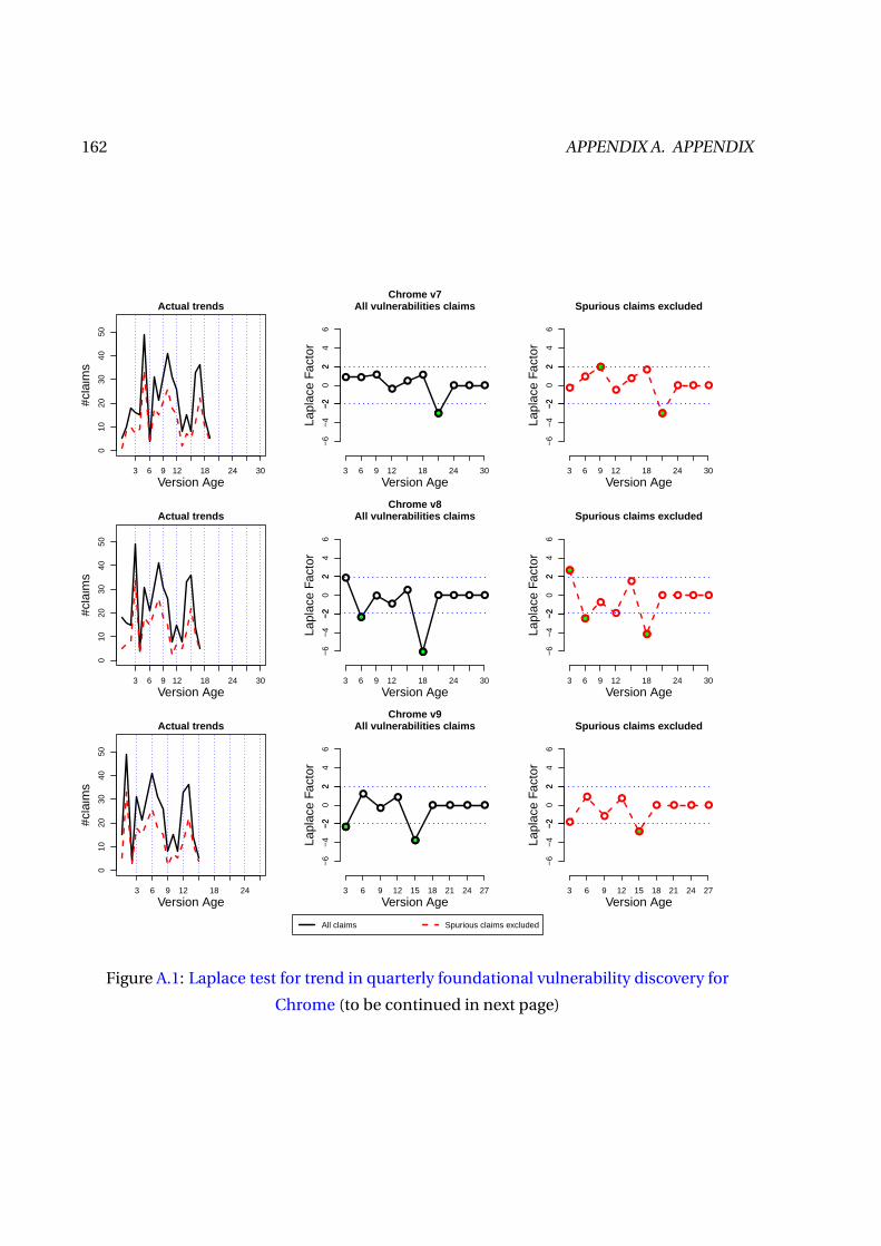
162 APPENDIX A. APPENDIX
010
2030
4050
Actual trends
3 6 9 12 18 24 30
#cla
ims
Version Age
−6
−4
−2
02
46
Chrome v7All vulnerabilities claims
−2
2
3 6 9 12 18 24 30
Lapl
ace
Fact
or
Version Age
−6
−4
−2
02
46
Spurious claims excluded
−2
2
3 6 9 12 18 24 30
Lapl
ace
Fact
or
Version Age
010
2030
4050
Actual trends
3 6 9 12 18 24 30
#cla
ims
Version Age
−6
−4
−2
02
46
Chrome v8All vulnerabilities claims
−2
2
3 6 9 12 18 24 30
Lapl
ace
Fact
or
Version Age
−6
−4
−2
02
46
Spurious claims excluded
−2
2
3 6 9 12 18 24 30
Lapl
ace
Fact
or
Version Age
010
2030
4050
Actual trends
3 6 9 12 18 24
#cla
ims
Version Age
−6
−4
−2
02
46
Chrome v9All vulnerabilities claims
−2
2
3 6 9 12 15 18 21 24 27
Lapl
ace
Fact
or
Version Age
−6
−4
−2
02
46
Spurious claims excluded
−2
2
3 6 9 12 15 18 21 24 27
Lapl
ace
Fact
or
Version Age
All claims Spurious claims excluded
Figure A.1: Laplace test for trend in quarterly foundational vulnerability discovery for
Chrome (to be continued in next page)

A.1. DETAILS OF LAPLACE TEST FOR QUARTERLY TRENDS OF FOUNDATIONALVULNERABILITIES 163
010
2030
4050
Actual trends
3 6 9 12 18 24
#cla
ims
Version Age
−6
−4
−2
02
46
Chrome v10All vulnerabilities claims
−2
2
3 6 9 12 15 18 21 24 27
Lapl
ace
Fact
or
Version Age
−6
−4
−2
02
46
Spurious claims excluded
−2
2
3 6 9 12 15 18 21 24 27
Lapl
ace
Fact
or
Version Age
010
2030
4050
Actual trends
3 6 9 12 15 18 21 24
#cla
ims
Version Age
−6
−4
−2
02
46
Chrome v11All vulnerabilities claims
−2
2
3 6 9 12 15 18 21 24
Lapl
ace
Fact
or
Version Age
−6
−4
−2
02
46
Spurious claims excluded
−2
2
3 6 9 12 15 18 21 24
Lapl
ace
Fact
or
Version Age
010
2030
4050
Actual trends
3 6 9 12 15 18 21 24
#cla
ims
Version Age
−6
−4
−2
02
46
Chrome v12All vulnerabilities claims
−2
2
3 6 9 12 15 18 21 24
Lapl
ace
Fact
or
Version Age
−6
−4
−2
02
46
Spurious claims excluded
−2
2
3 6 9 12 15 18 21 24
Lapl
ace
Fact
or
Version Age
All claims Spurious claims excluded
Figure A.1: Laplace test for trend in quarterly foundational vulnerability discovery for
Chrome (to be continued in next page)

164 APPENDIX A. APPENDIX
010
2030
4050
Actual trends
3 6 9 12 15 18 21
#cla
ims
Version Age
−6
−4
−2
02
46
Chrome v13All vulnerabilities claims
−2
2
3 6 9 12 15 18 21
Lapl
ace
Fact
or
Version Age
−6
−4
−2
02
46
Spurious claims excluded
−2
2
3 6 9 12 15 18 21
Lapl
ace
Fact
or
Version Age
010
2030
4050
Actual trends
3 6 9 12 15 18 21
#cla
ims
Version Age
−6
−4
−2
02
46
Chrome v14All vulnerabilities claims
−2
2
3 6 9 12 15 18 21
Lapl
ace
Fact
or
Version Age
−6
−4
−2
02
46
Spurious claims excluded
−2
2
3 6 9 12 15 18 21
Lapl
ace
Fact
or
Version Age
010
2030
4050
Actual trends
3 6 9 12 15 18
#cla
ims
Version Age
−6
−4
−2
02
46
Chrome v15All vulnerabilities claims
−2
2
3 6 9 12 15 18
Lapl
ace
Fact
or
Version Age
−6
−4
−2
02
46
Spurious claims excluded
−2
2
3 6 9 12 15 18
Lapl
ace
Fact
or
Version Age
All claims Spurious claims excluded
Figure A.1: Laplace test for trend in quarterly foundational vulnerability discovery for
Chrome (to be continued in next page)

A.1. DETAILS OF LAPLACE TEST FOR QUARTERLY TRENDS OF FOUNDATIONALVULNERABILITIES 165
010
2030
4050
Actual trends
3 6 9 12 15 18
#cla
ims
Version Age
−6
−4
−2
02
46
Chrome v16All vulnerabilities claims
−2
2
3 6 9 12 15 18
Lapl
ace
Fact
or
Version Age
−6
−4
−2
02
46
Spurious claims excluded
−2
2
3 6 9 12 15 18
Lapl
ace
Fact
or
Version Age
010
2030
4050
Actual trends
3 6 9 12 15
#cla
ims
Version Age
−6
−4
−2
02
46
Chrome v17All vulnerabilities claims
−2
2
3 6 9 12 15
Lapl
ace
Fact
or
Version Age
−6
−4
−2
02
46
Spurious claims excluded
−2
2
3 6 9 12 15
Lapl
ace
Fact
or
Version Age
010
2030
4050
Actual trends
3 6 9 12 15
#cla
ims
Version Age
−6
−4
−2
02
46
Chrome v18All vulnerabilities claims
−2
2
3 6 9 12 15
Lapl
ace
Fact
or
Version Age
−6
−4
−2
02
46
Spurious claims excluded
−2
2
3 6 9 12 15
Lapl
ace
Fact
or
Version Age
All claims Spurious claims excluded
Figure A.1: Laplace test for trend in quarterly foundational vulnerability discovery for
Chrome (continued from previous pages)

166 APPENDIX A. APPENDIX
010
2030
4050
Actual trends
3 15 27 39 51 63 75 87 99
#cla
ims
Version Age
−6
−4
−2
02
46
Firefox v1.0All vulnerabilities claims
−2
2
3 15 27 39 51 63 75 87 99
Lapl
ace
Fact
or
Version Age
−6
−4
−2
02
46
Spurious claims excluded
−2
2
3 15 27 39 51 63 75 87 99
Lapl
ace
Fact
or
Version Age
010
2030
4050
Actual trends
3 12 24 36 48 60 72 84
#cla
ims
Version Age
−6
−4
−2
02
46
Firefox v1.5All vulnerabilities claims
−2
2
3 12 24 36 48 60 72 84
Lapl
ace
Fact
or
Version Age
−6
−4
−2
02
46
Spurious claims excluded
−2
2
3 12 24 36 48 60 72 84
Lapl
ace
Fact
or
Version Age
010
2030
4050
Actual trends
3 12 24 36 48 60 72
#cla
ims
Version Age
−6
−4
−2
02
46
Firefox v2.0All vulnerabilities claims
−2
2
3 12 21 30 39 48 57 66 75
Lapl
ace
Fact
or
Version Age
−6
−4
−2
02
46
Spurious claims excluded
−2
2
3 12 21 30 39 48 57 66 75
Lapl
ace
Fact
or
Version Age
All claims Spurious claims excluded
Figure A.2: Laplace test for trend in quarterly foundational vulnerability discovery for Firefox
(to be continued in next page)

A.1. DETAILS OF LAPLACE TEST FOR QUARTERLY TRENDS OF FOUNDATIONALVULNERABILITIES 167
010
2030
4050
Actual trends
3 9 15 24 33 42 51 60
#cla
ims
Version Age
−6
−4
−2
02
46
Firefox v3.0All vulnerabilities claims
−2
2
3 9 15 24 33 42 51 60
Lapl
ace
Fact
or
Version Age
−6
−4
−2
02
46
Spurious claims excluded
−2
2
3 9 15 24 33 42 51 60
Lapl
ace
Fact
or
Version Age
010
2030
4050
Actual trends
3 9 15 21 27 33 39 45
#cla
ims
Version Age
−6
−4
−2
02
46
Firefox v3.5All vulnerabilities claims
−2
2
3 9 15 21 27 33 39 45
Lapl
ace
Fact
or
Version Age
−6
−4
−2
02
46
Spurious claims excluded
−2
2
3 9 15 21 27 33 39 45
Lapl
ace
Fact
or
Version Age
010
2030
4050
Actual trends
3 9 15 21 27 33 39
#cla
ims
Version Age
−6
−4
−2
02
46
Firefox v3.6All vulnerabilities claims
−2
2
3 6 9 15 21 27 33 39
Lapl
ace
Fact
or
Version Age
−6
−4
−2
02
46
Spurious claims excluded
−2
2
3 6 9 15 21 27 33 39
Lapl
ace
Fact
or
Version Age
All claims Spurious claims excluded
Figure A.2: Laplace test for trend in quarterly foundational vulnerability discovery for
Firefox (to be continued in next page)

168 APPENDIX A. APPENDIX
010
2030
4050
Actual trends
3 6 9 12 15 18 21 24
#cla
ims
Version Age
−6
−4
−2
02
46
Firefox v4.0All vulnerabilities claims
−2
2
3 6 9 12 15 18 21 24
Lapl
ace
Fact
or
Version Age
−6
−4
−2
02
46
Spurious claims excluded
−2
2
3 6 9 12 15 18 21 24
Lapl
ace
Fact
or
Version Age
010
2030
4050
Actual trends
3 6 9 12 15 18 21
#cla
ims
Version Age
−6
−4
−2
02
46
Firefox v5.0All vulnerabilities claims
−2
2
3 6 9 12 15 18 21
Lapl
ace
Fact
or
Version Age
−6
−4
−2
02
46
Spurious claims excluded
−2
2
3 6 9 12 15 18 21
Lapl
ace
Fact
or
Version Age
010
2030
4050
Actual trends
3 6 9 12 15 18 21
#cla
ims
Version Age
−6
−4
−2
02
46
Firefox v6.0All vulnerabilities claims
−2
2
3 6 9 12 15 18 21
Lapl
ace
Fact
or
Version Age
−6
−4
−2
02
46
Spurious claims excluded
−2
2
3 6 9 12 15 18 21
Lapl
ace
Fact
or
Version Age
All claims Spurious claims excluded
Figure A.2: Laplace test for trend in quarterly foundational vulnerability discovery for
Firefox (to be continued in next page)

A.1. DETAILS OF LAPLACE TEST FOR QUARTERLY TRENDS OF FOUNDATIONALVULNERABILITIES 169
010
2030
4050
Actual trends
3 6 9 12 15 18
#cla
ims
Version Age
−6
−4
−2
02
46
Firefox v7.0All vulnerabilities claims
−2
2
3 6 9 12 15 18
Lapl
ace
Fact
or
Version Age
−6
−4
−2
02
46
Spurious claims excluded
−2
2
3 6 9 12 15 18
Lapl
ace
Fact
or
Version Age
010
2030
4050
Actual trends
3 6 9 12 15 18
#cla
ims
Version Age
−6
−4
−2
02
46
Firefox v8.0All vulnerabilities claims
−2
2
3 6 9 12 15 18
Lapl
ace
Fact
or
Version Age
−6
−4
−2
02
46
Spurious claims excluded
−
22
3 6 9 12 15 18
Lapl
ace
Fact
or
Version Age
010
2030
4050
Actual trends
3 6 9 12 15
#cla
ims
Version Age
−6
−4
−2
02
46
Firefox v9.0All vulnerabilities claims
−2
2
3 6 9 12 15
Lapl
ace
Fact
or
Version Age
−6
−4
−2
02
46
Spurious claims excluded
−2
2
3 6 9 12 15
Lapl
ace
Fact
or
Version Age
All claims Spurious claims excluded
Figure A.2: Laplace test for trend in quarterly foundational vulnerability discovery for
Firefox (to be continued in next page)
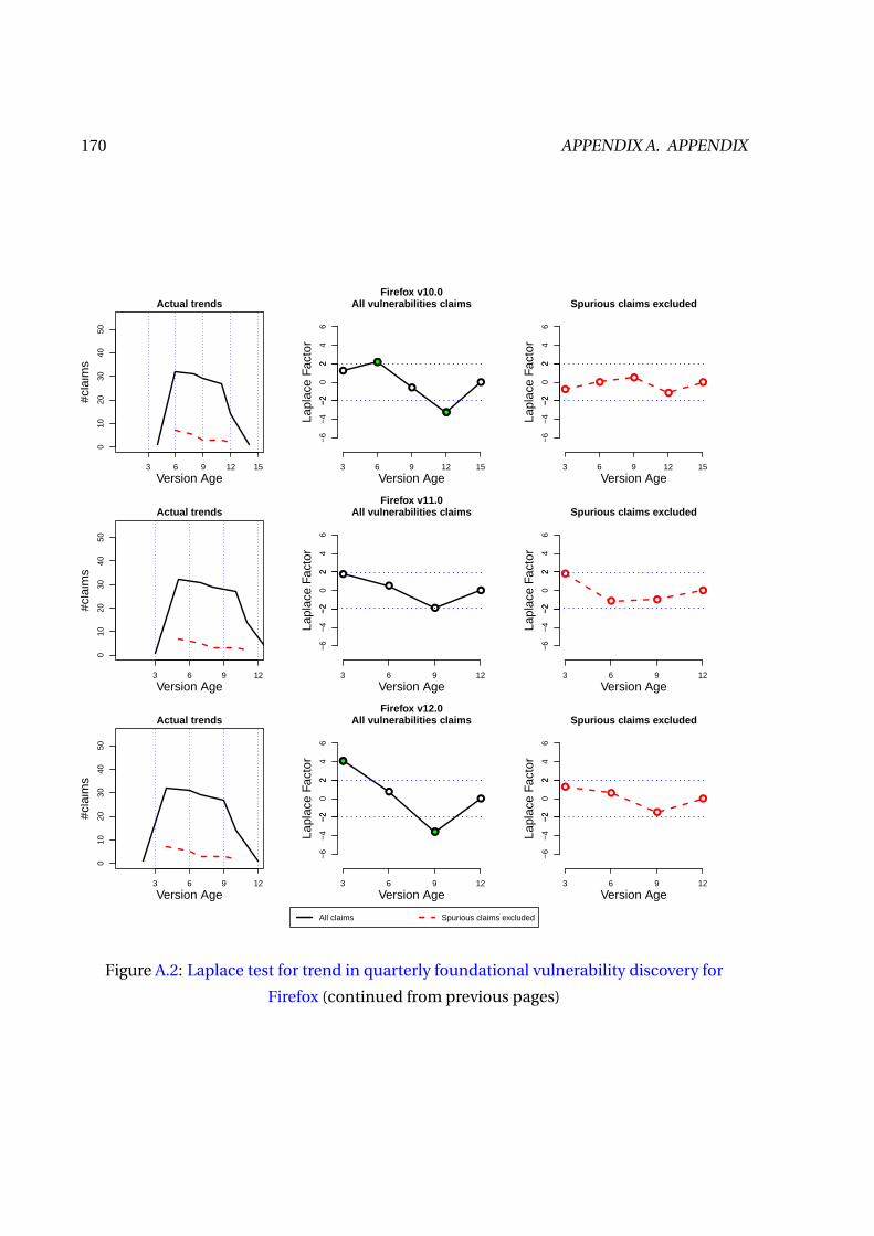
170 APPENDIX A. APPENDIX
010
2030
4050
Actual trends
3 6 9 12 15
#cla
ims
Version Age
−6
−4
−2
02
46
Firefox v10.0All vulnerabilities claims
−2
2
3 6 9 12 15
Lapl
ace
Fact
or
Version Age
−6
−4
−2
02
46
Spurious claims excluded
−2
2
3 6 9 12 15
Lapl
ace
Fact
or
Version Age
010
2030
4050
Actual trends
3 6 9 12
#cla
ims
Version Age
−6
−4
−2
02
46
Firefox v11.0All vulnerabilities claims
−2
2
3 6 9 12
Lapl
ace
Fact
or
Version Age
−6
−4
−2
02
46
Spurious claims excluded
−2
2
3 6 9 12
Lapl
ace
Fact
or
Version Age
010
2030
4050
Actual trends
3 6 9 12
#cla
ims
Version Age
−6
−4
−2
02
46
Firefox v12.0All vulnerabilities claims
−2
2
3 6 9 12
Lapl
ace
Fact
or
Version Age
−6
−4
−2
02
46
Spurious claims excluded
−2
2
3 6 9 12
Lapl
ace
Fact
or
Version Age
All claims Spurious claims excluded
Figure A.2: Laplace test for trend in quarterly foundational vulnerability discovery for
Firefox (continued from previous pages)

A.1. DETAILS OF LAPLACE TEST FOR QUARTERLY TRENDS OF FOUNDATIONALVULNERABILITIES 171
Table A.1: Inconsistent events in Laplace test for quarterly trends in Chrome.
Numbers in the second and third columns are the version ages (in month) when the
Laplace factors indicate significant trends.
Inconsistent Events
Release NVD data set Verified NVD data set Count
Chrome v1 18, 21 36 3
Chrome v2 27 – 1
Chrome v3 12 21 2
Chrome v4 – 27 1
Chrome v5 15, 24 3 3
Chrome v6 6, 15 2
Chrome v7 – 9 1
Chrome v8 – 3 1
Chrome v9 3 – 1
Chrome v10 – – 0
Chrome v11 – 3, 12 2
Chrome v12 – 6 1
Chrome v13 – – 0
Chrome v14 – – 0
Chrome v15 – – 0
Chrome v16 – – 0
Chrome v17 – – 0
Chrome v18 – – 0

172 APPENDIX A. APPENDIX
Table A.2: Inconsistent events in Laplace test for quarterly trends in Firefox.
Numbers in the second and third columns are the version ages (in month) when the
Laplace factors indicate significant trends.
Inconsistent Events
Release NVD data set Verified NVD data set Count
Firefox v1.0 93, 99 30, 54, 69 5
Firefox v1.5 57, 81, 87 – 3
Firefox v2.0 69, 75 – 2
Firefox v3.0 9, 57 – 2
Firefox v3.5 42 24 2
Firefox v3.6 27 – 1
Firefox v4.0 21 – 1
Firefox v5.0 18 – 1
Firefox v6.0 18 – 1
Firefox v7.0 9, 15 – 2
Firefox v8.0 9, 15 – 2
Firefox v9.0 6, 12 – 2
Firefox v10.0 6, 12 – 2
Firefox v11.0 – – 0
Firefox v12.0 3, 9 – 2