wald tests for detecting multiple structural changes in persistence
TRANSCRIPT

7/25/2019 WALD TESTS FOR DETECTING MULTIPLE STRUCTURAL CHANGES IN PERSISTENCE
http://slidepdf.com/reader/full/wald-tests-for-detecting-multiple-structural-changes-in-persistence 1/35
Econometric Theory, 2012, Page 1 of 35.doi:10.1017/S0266466612000357
WALD TESTS FOR DETECTING
MULTIPLE STRUCTURAL
CHANGES IN PERSISTENCE
MOHITOSH KEJRIWAL
Purdue University
PIERRE PERRON
Boston University
JING
ZHOU
Orient Securities Company Limited
This paper considers the problem of testing for multiple structural changes in the per-
sistence of a univariate time series. We propose sup-Wald tests of the null hypothesis
that the process has an autoregressive unit root throughout the sample against the
alternative hypothesis that the process alternates between stationary and unit root
regimes. We derive the limit distributions of the tests under the null and establish
their consistency under the relevant alternatives. We further show that the tests are
inconsistent when directed against the incorrect alternative, thereby enabling iden-
tification of the nature of persistence in the initial regime. We also propose hybrid
testing procedures that allow ruling out of stable stationary processes or ones that
are subject to only stationary changes under the null, thereby aiding the researcher
in interpreting a rejection as emanating from a switch between a unit root and sta-
tionary regime. The computation of the test statistics as well as asymptotic critical
values is facilitated by the dynamic programming algorithm proposed in Perron and
Qu (2006, Journal of Econometrics 134, 373–399) which allows imposing within-
and cross-regime restrictions on the parameters. Finally, we present Monte Carlo
evidence to show that the proposed procedures perform well in finite samples rela-
tive to those available in the literature.
1. INTRODUCTION
Issues related to the detection and estimation of structural change in time series
models have received a great deal of attention in both the statistics and economet-
rics literature (see Perron, 2006, for a survey). Substantial advances have been
Perron acknowledges financial support for this work from the National Science Foundation under Grant
SES-0649350. The authors are grateful to Robert Taylor (the co-editor) and two anonymous referees for use-
ful comments and suggestions that helped improve the paper. Address correspondence to Mohitosh Kejriwal,
Krannert School of Management, Purdue University, 403 West State Street, West Lafayette IN 47907 USA; e-mail:
c Cambridge University Press 2012 1
7/25/2019 WALD TESTS FOR DETECTING MULTIPLE STRUCTURAL CHANGES IN PERSISTENCE
http://slidepdf.com/reader/full/wald-tests-for-detecting-multiple-structural-changes-in-persistence 2/35
2 MOHITOSH KEJRIWAL ET AL.
made to cover models at a level of generality that allows a host of interesting
empirical applications. These include models with general stationary regressors,
models with trending variables and possible unit roots, cointegrated models, and
long memory processes, among others. Also of interest is the interplay betweenstructural changes and unit roots (Perron, 1989). The literature on testing for a
change in the persistence of a time series is less extensive and relatively recent. If
such a change preserves the stationarity properties of the series in the respective
regimes, methods developed in the context of stationary data can still be applied
(see Andrews, 1993; Bai and Perron, 1998; 2003). In many cases, however, a
process may switch from one with an autoregressive unit root [ I (1)] to a sta-
tionary one [ I (0)] or vice versa. This has been an issue of substantial empirical
interest, especially concerning inflation rate series (e.g., Barsky, 1987; Burdekin
and Siklos, 1999), short-term interest rates (e.g., Mankiw, Miron, and Wei, 1987),government budget deficits (e.g., Hakkio and Rush, 1991), and real output (e.g.,
Delong and Summers, 1988). Kim (2003) shows that standard unit root tests are
not consistent against processes displaying a shift from stationarity to nonstation-
arity and vice versa. Hence, separate methods are needed to distinguish between a
process with stable persistence and one that undergoes a shift in persistence over
a given period.
Kim (2000), Busetti and Taylor (2004), and Taylor (2005) consider testing the
null hypothesis that the series is I (0) throughout the sample versus the alternative
that it switches from I (0) to I (1) and vice versa. Harvey, Leybourne, and Taylor(2006) propose test statistics that allow the process to be I (1) or I (0) through-
out under the null. The tests are based on partial sums of residuals obtained by
regressing the data on a constant or a constant and time trend. Leybourne, Kim,
Smith, and Newbold (2003) consider testing the null hypothesis of a stable unit
root process versus the same alternatives based on the minimal value of the locally
generalized least squares (GLS) detrended augmented Dickey-Fuller ( ADF ) unit
root statistic developed in Elliott, Rothenberg, and Stock (1996) over subsamples
of the data. They propose different test statistics depending on whether the initial
regime is I (1) or I (0). When the direction of the change is unknown, they con-sider the minimal value of the pair of statistics for each case. Kurozumi (2005)
suggests an alternative testing procedure based on the Lagrange multiplier (LM)
principle, while Leybourne, Kim, and Taylor (2007a) develop tests of the unit root
null based on standardized cumulative sums of squared subsample residuals that
do not spuriously reject when the series is a constant I (0) process. Chong (2001)
studies the asymptotic properties of the estimated parameters in the first-order
autoregressive model with a single break in persistence.
The above tests are designed to detect a single change in persistence and do not
allow for multiple changes. Single break tests usually have low power in detect-ing processes that display multiple shifts in persistence. It is thus useful to develop
tests that are valid in the presence of multiple structural changes. In a recent paper,
Leybourne, Kim, and Taylor (2007b) develop tests of the unit root null hypoth-
esis based on doubly recursive sequences of ADF -type unit root statistics and

7/25/2019 WALD TESTS FOR DETECTING MULTIPLE STRUCTURAL CHANGES IN PERSISTENCE
http://slidepdf.com/reader/full/wald-tests-for-detecting-multiple-structural-changes-in-persistence 3/35
DETECTING MULTIPLE CHANGES IN PERSISTENCE 3
associated breakpoint estimators. Their proposed procedure can accommodate
processes that exhibit multiple changes in persistence and are valid regardless
of the direction of change(s). In particular, they demonstrate the consistency of
their tests against such alternatives and show that their procedure can be used toconsistently partition the data into its separate I (0) and I (1) regimes. Kang, Kim,
and Morley (2009) consider an alternative approach to analyzing multiple regime
shifts in U.S. inflation persistence based on an unobserved components model
with Markov-switching parameters.
As is evident from this brief review, most tests for changes in persistence are
based on either partial sums of the (demeaned or detrended) data or on unit root
statistics applied to various data subsamples. In contrast, this paper proposes
sup-Wald tests of the null hypothesis that the process is I (1) against the alterna-
tive hypothesis that the process alternates between stationary and I (1) regimes.The tests are based on the difference between the sum of squared residuals
from the unit root model and those from a model that allows shifts in persis-
tence between stationary and nonstationary regimes. We consider tests for both
single and multiple changes in persistence. The limit distributions of the tests
are derived under the null, and their consistency is established under the rele-
vant alternatives. We further show that the tests are inconsistent when directed
against the incorrect alternative, thereby allowing the researcher to identify the
nature of persistence in the initial regime. We also propose hybrid testing pro-
cedures that allow ruling out of stable stationary processes or ones that are aresubject to only stationary changes under the null, thereby aiding the researcher
in interpreting a rejection as emanating from a switch between a unit root and
stationary regime. We further discuss how our tests can be used to distinguish
between persistence breaks and pure level or trend breaks. The computation of
the test statistics as well as asymptotic critical values is facilitated by the dy-
namic programming algorithm proposed in Perron and Qu (2006), which allows
the minimization of the sum of squared residuals under the alternative hypothe-
sis while imposing within- and cross-regime restrictions on the parameters. We
also propose estimators for the break dates that can be employed once evidenceagainst a stable persistence parameter is obtained. The performance of the pro-
posed test statistics in small samples is evaluated via an extensive Monte Carlo
study.
The paper is organized as follows. Section 2 presents the models, the test statis-
tics, and issues related to the computation of the statistics. Section 3 details the
asymptotic properties of the test statistics under the null and alternative hypothe-
ses. Section 4 proposes hybrid testing procedures that allow ruling out processes
that are constant I (0) or ones that are subject to only I (0) changes under the null.
Section 5 suggests estimators for the locations of the break points that can be ap-plied following evidence against the null hypothesis. Monte Carlo simulations are
presented in Section 6 to assess the adequacy of the asymptotic approximations
in finite samples. Recommendations for applied work are also included. Section 7
concludes. All technical derivations are in the Appendix.
7/25/2019 WALD TESTS FOR DETECTING MULTIPLE STRUCTURAL CHANGES IN PERSISTENCE
http://slidepdf.com/reader/full/wald-tests-for-detecting-multiple-structural-changes-in-persistence 4/35
4 MOHITOSH KEJRIWAL ET AL.
2. THE MODELS AND TEST STATISTICS
Consider a scalar random variable yt generated by
yt = ci + αi yt −1 + ui t (1)
for t ∈ [T i −1 + 1, T i ], i = 1, . . . , m + 1, with the convention that T 0 = 0 and
T m+1 = T , where T is the sample size. The vector of break fractions is λ =
(λ1, . . . , λm ) with λi = T i /T for i = 1, . . . , m. Hence, we have m breaks and m + 1
regimes that increase in length in the same proportion as T increases. The errors
{ui t } are generated by the stationary linear process
ui t = d i ( L)v i t , d i ( L) =∞
∑s=0
d is Ls , (2)
where ∑∞s=1 s |d is | < ∞. Also, αi should be understood as standing for the sum of
the coefficients in the autoregressive representation for yt in regime i . We make
the following assumptions regarding the innovation process {v i t } and u i t for i =
1, . . . , m + 1.
Assumption A1. The process {v i t } is a martingale difference sequence
with E(v 2i t |v i t −1,. . .) = σ 2, E(|v i t |
r |v i t −1,...) = κir (r = 3, 4), and supt
E(|v i t |4+ β |v i t −1,...) = κi < ∞ for some β > 0.
Assumption A2. All roots of d i ( L) are outside the unit circle.
We consider the following two models depending on whether the initial regime
contains a unit root or not: Model 1a: ci = 0, αi = 1 in odd regimes and |αi | < 1 in
even regimes; Model 1b: ci = 0, αi = 1 in even regimes and |αi | < 1 in odd
regimes. In Model 1a, the process alternates between a unit root and a stationary
process with a unit root in the first regime. Model 1b is similar except that the first
regime is stationary. To allow for the possibility of trending data, we also consider
the process
yt = ci + bi t + αi yt −1 + ui t .
The corresponding models are: Model 2a: αi = 1, bi = 0 in odd regimes and
|αi | < 1 in even regimes; Model 2b: αi = 1, bi = 0 in even regimes and |αi | < 1
in odd regimes. We are interested in testing the null hypothesis that yt is I (1)
throughout the sample. For Models 1a and 1b, this implies H 0: ci = 0, αi = 1 for
all i . For Models 2a and 2b, the null hypothesis is H 0: ci = c, bi = 0, αi = 1 for
all i . In this case, the data generating process (DGP) is denoted by
yt = c + yt −1 + ut , (3)
where u t = d ( L)v t , d ( L) = ∑∞s=0 d s Ls with v t and d ( L) satisfying Assumptions
A1–A2 and ∑∞s=1 s|d s | < ∞.
7/25/2019 WALD TESTS FOR DETECTING MULTIPLE STRUCTURAL CHANGES IN PERSISTENCE
http://slidepdf.com/reader/full/wald-tests-for-detecting-multiple-structural-changes-in-persistence 5/35
DETECTING MULTIPLE CHANGES IN PERSISTENCE 5
It is important to note that under the alternative hypothesis the process gener-
ating the data is such that all parameters are allowed to change across regimes.
Hence, level shifts and changes in the slope of the trend are allowed, as well as
changes in the dynamics and the variance of the errors. We, however, shall notconstruct test statistics that exploit the possible changes in the dynamics or the
variance of the errors. This is because we wish to direct the test against potential
changes in the I(0)/I(1) nature of the process to ensure the highest power possible.
Also, allowing for breaks in dynamics under the null would lead to limit distribu-
tions that depend on the (unknown) number and location of these breaks, thereby
making asymptotic inference difficult. A joint test on all parameters would not be
particularly informative given the difficulty in interpreting a rejection. As shown
in Section 6.2, our test does not have much power against pure changes in short-
run dynamics but is powerful when there is a change in both persistence and thesedynamics. We nevertheless allow for concurrent changes in level and slope of the
trend function, since these often occur simultaneously with a change in persis-
tence and can allow tests with higher power.
We first consider the test statistics for nontrending data, i.e., those based on
Models 1a and 1b. Given the fact that the process has an autoregressive represen-
tation that can be approximated by an A R(lT ) for some sequence lT increasing
with the sample size, the starting point is to consider the regression
yt = ci + (αi − 1) yt −1 +
lT
∑ j=1
π j yt − j + v ∗t . (4)
In accordance with the discussion above, the coefficients π j pertaining to the dy-
namics are not allowed to change across regimes. Also, the tests are based on the
constrained and unconstrained sum of squared residuals, which follows a least-
squares approach that does not exploit potential changes in the variance of the
errors.
We study two types of tests in this section. First, we consider the Wald test that
applies when the alternative involves a fixed value m = k of changes. For Models
1a–1b, the test is defined as
F 1a (λ, k ) = (T − k − lT )(S S R0 − SS R1a,k )/[k S S R1a,k ] if k is even,
F 1a (λ, k ) = (T − k − 1 − lT )(S S R0 − SS R1a,k )/[(k + 1)SS R1a,k ] if k is odd,
(5)
F 1b(λ, k ) = (T − k − 2 − lT )(S S R0 − SS R1b,k )/[(k + 2)SS R1b,k ] if k is even,
F 1b(λ, k ) = (T − k − 1 − lT )(S S R0 − SS R1b,k )/[(k + 1)SS R1b,k ] if k is odd.
(6)
In (5) and (6), S S R0 denotes the sum of squared residuals under the null hy-
pothesis, i.e., that obtained from ordinary least squares (OLS) estimation of
(4) subject to the restrictions ci = 0, αi = 1 for all i . S S Rk ,1a denotes the sum of
squared residuals obtained from estimating (4) under the restrictions imposed by
7/25/2019 WALD TESTS FOR DETECTING MULTIPLE STRUCTURAL CHANGES IN PERSISTENCE
http://slidepdf.com/reader/full/wald-tests-for-detecting-multiple-structural-changes-in-persistence 6/35
6 MOHITOSH KEJRIWAL ET AL.
Model 1a. Similarly, S S Rk ,1b denotes the sum of squared residuals obtained from
estimating (4) under the restrictions imposed by Model 1b. For some arbitrary
small positive number , we define the set k = {λ : |λi +1 − λi | ≥ , λ 1 ≥ , λ k ≤
1−}. The sup-Wald tests are then defined as sup F 1a(k ) = supλ ∈k F 1a(λ, k ) andsup F 1b(k ) = supλ ∈k
F 1b(λ, k ). Note that to ensure that the Wald tests are
nonnegative, the same number of lags of the first differences of the dependent
variable must be used when estimating the models under the null and alternative
hypotheses, another reason not to model the changes in the dynamics.
The second type of test is based on the presumption that the nature of persis-
tence in the first regime is unknown, i.e., we do not have any a priori knowledge
regarding whether the first regime contains a unit root or not. The tests are given
by W 1(k ) = max[sup F 1a(λ, k ), sup F 1b(λ, k )]. Finally, in order to accommodate
the case with an unknown number of breaks, up to some maximal value A, weconsider the statistic W max1 = max1≤m≤ A W 1(m). For models 2a and 2b, regres-
sion (4) is replaced by
yt = ci + bi t + (αi − 1) yt −1 +lT
∑ j =1
π j yt − j + v ∗t . (7)
The Wald tests are defined as
F 2a (λ, k ) = (T − 2k − 1 − lT )(S S R∗0 − S S R2a,k )/[(2k )S S R2a,k ] if k is even,
F 2a (λ, k ) = (T − 2k − 2 − lT )(S S R∗0 − S S R2a,k )/[(2k + 1)S S R2a,k ] if k is odd,
(8)
F 2b(λ, k ) = (T − 2k − 3 − lT )(S S R∗0 − S S R2b,k )/[(2k + 2)S S R2b,k ] if k is even,
F 2b(λ, k ) = (T − 2k − 2 − lT )(S S R∗0 − S S R2b,k )[(2k + 1)SS R2b,k ] if k is odd.
(9)
In (8) and (9), S S R∗0 denotes the sum of squared residuals under the null hy-
pothesis, i.e., the sum of squared residuals obtained estimating (7) subject to therestrictions ci = c, bi = 0, αi = 1 for all i . Given these tests, the remaining statis-
tics are defined in the same way as for Models 1a and 1b. These are denoted sup
F 2a (k ), sup F 2b(k ), W 2(k ), and W max2. To compute the sup-Wald test for any
particular model, we need to minimize the global sum of squared residuals over
the set of permissible break fractions k subject to the restrictions implied by the
model. This is accomplished employing the dynamic programming algorithm of
Perron and Qu (2006).
3. ASYMPTOTIC RESULTS
We now consider the limiting properties of the proposed statistics. In 3.1 we
present the asymptotic distributions of the tests under the null hypothesis that the
process is I (1) throughout the sample. The computation of the asymptotic critical
7/25/2019 WALD TESTS FOR DETECTING MULTIPLE STRUCTURAL CHANGES IN PERSISTENCE
http://slidepdf.com/reader/full/wald-tests-for-detecting-multiple-structural-changes-in-persistence 7/35
DETECTING MULTIPLE CHANGES IN PERSISTENCE 7
values is discussed in 3.2, and in 3.3 we demonstrate the consistency of the tests
under the relevant alternative hypotheses.
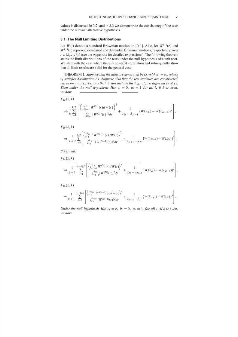
3.1. The Null Limiting Distributions
Let W (.) denote a standard Brownian motion on [0, 1]. Also, let W ( j )(r ) andW ( j )(r ) represent demeaned and detrended Brownian motions, respectively, over
r ∈ (λ j−1, λ j ) (see the Appendix for detailed expressions). The following theorem
states the limit distributions of the tests under the null hypothesis of a unit root.
We start with the case where there is no serial correlation and subsequently show
that all limit results are valid for the general case.
THEOREM 1. Suppose that the data are generated by (3) with ut = v t , where
v t satisfies Assumption A1. Suppose also that the test statistics are constructed based on autoregressions that do not include the lags of first differences of y t .
Then under the null hypothesis H 0: ci = 0, αi = 1 for all i, if k is even,
we have
F 1a (λ, k )
⇒ 1
k
k /2
∑i =1
λ2i
λ2i−1W (2i )(r )d W (r )
2
λ2i
λ2i−1[W (2i )(r )]2dr
+ 1
λ2i − λ2i −1
{W (λ2i ) − W (λ2i−1)}2
,
F 1b(λ, k )
⇒ 1
k + 2
k /2
∑i =0
λ2i +1
λ2iW (2i +1)(r )d W (r )
2
λ2i +1
λ2i[W (2i +1)(r )]2dr
+ 1
λ2i +1 − λ2i
{W (λ2i +1) − W (λ2i )}2
.
If k is odd,
F 1a (λ, k )
⇒ 1
k + 1
(k +1)/2
∑i =1
λ2i
λ2i −1W (2i )(r )dW (r )
2
λ2iλ2i −1
[W (2i )(r )]2dr +
1
λ2i − λ2i −1
{W (λ2i ) − W (λ2i−1)}2
,
F 1b(λ, k )
⇒ 1
k + 1
(k −1)/2
∑i=0
λ2i +1
λ2iW (2i +1)(r )d W (r )
2
λ2i +1
λ2i[W (2i +1)(r )]2dr
+ 1
λ2i +1 − λ2iW (λ2i+1) − W (λ2i )2 .
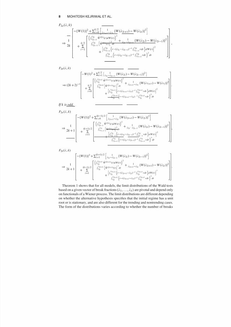
Under the null hypothesis H 0: ci = c, bi = 0, αi = 1 for all i, if k is even,
we have
7/25/2019 WALD TESTS FOR DETECTING MULTIPLE STRUCTURAL CHANGES IN PERSISTENCE
http://slidepdf.com/reader/full/wald-tests-for-detecting-multiple-structural-changes-in-persistence 8/35
8 MOHITOSH KEJRIWAL ET AL.
F 2a(λ, k )
⇒ 1
2k
−{W (1)}2 +∑k /2i =0
1
λ2i +1−λ2i{W (λ2i+1) − W (λ2i )}2
+
k /2
∑i =1
λ2iλ2i −1 W (2i)(r )d W (r )2
λ2iλ2i −1
W (2i )(r )2
dr + 1
λ2i −λ2i −1{W (λ2i ) − W (λ2i−1)}2
+
λ2iλ2i−1
r −(λ2i −λ2i−1)−1
λ2iλ2i −1
r dr
d W (r )2
λ2iλ2i−1
r −(λ2i −λ2i −1)−1
λ2iλ2i−1
r dr 2
dr
,
F 2b(λ, k )
⇒ (2k + 2)−1
−W (1)2 +∑k /2
i =1 1
λ2i −λ2i−1
{W (λ2i ) − W (λ2i −1)}2 +
k /2
∑i =0
λ2i +1
λ2iW (2i+1)(r )d W (r )
2
λ2i+1λ2i
W (2i +1)(r )2
dr
+ 1λ2i +1−λ2i
{W (λ2i +1) − W (λ2i )}2
+
λ2i+1λ2i
r −(λ2i +1−λ2i )−1
λ2i +1λ2i
r dr
d W (r )2
λ2i +1λ2i
r −(λ2i+1−λ2i )−1
λ2i+1λ2i
r dr 2
dr
.
If k is odd,
F 2a (λ, k )
⇒ 1
2k + 1
−{W (1)}2 +∑(k −1)/2i =0
1λ2i+1−λ2i
{W (λ2i+1) − W (λ2i )}2
+(k +1)/2
∑i=1
λ2i
λ2i −1W (2i )(r )d W (r )
2
λ2iλ2i−1
W (2i )(r )2
dr + 1
λ2i −λ2i −1{W (λ2i ) − W (λ2i−1)}2
+
λ2iλ2i −1
r −(λ2i −λ2i −1)−1
λ2iλ2i −1
r dr
d W (r )
2
λ2iλ2i−1
r −(λ2i −λ2i −1)−1
λ2iλ2i −1
r dr
2dr
,
F 2b(λ, k )
⇒ 1
2k + 1
−{W (1)}2 +∑(k +1)/2i =1
1λ2i −λ2i−1
{W (λ2i ) − W (λ2i −1)}2
+(k −1)/2
∑i =1
λ2i+1
λ2iW (2i +1)(r )d W (r )
2
λ2i+1λ2i
W (2i+1)(r )2
dr + 1
λ2i+1−λ2i{W (λ2i +1) − W (λ2i )}2
+
λ2i +1λ2i
r −(λ2i+1−λ2i )−1
λ2i+1λ2i
r dr
d W (r )2
λ2i+1λ2i
r −(λ2i+1−λ2i )−1
λ2i+1λ2i
r dr 2
dr
.
Theorem 1 shows that for all models, the limit distributions of the Wald tests
based on a given vector of break fractions (λ1, . . . , λk ) are pivotal and depend onlyon functionals of a Wiener process. The limit distributions are different depending
on whether the alternative hypothesis specifies that the initial regime has a unit
root or is stationary, and are also different for the trending and nontrending cases.
The form of the distributions varies according to whether the number of breaks
7/25/2019 WALD TESTS FOR DETECTING MULTIPLE STRUCTURAL CHANGES IN PERSISTENCE
http://slidepdf.com/reader/full/wald-tests-for-detecting-multiple-structural-changes-in-persistence 9/35
DETECTING MULTIPLE CHANGES IN PERSISTENCE 9
under the alternative hypothesis is even or odd. With these theoretical results, we
can obtain the limit distributions of the proposed tests as a direct consequence of
the continuous mapping theorem.
COROLLARY 1. Denote the limit distribution of the test F j (λ, k ) by
F ∗ j (λ, k ) , j = 1a, 1b, 2a, 2b. Then, under the same null hypothesis as in
Theorem 1, we have (a) supλ∈k
F j (λ, k ) ⇒ supλ∈k
F ∗ j (λ, k ); (b) W 1(k ) ⇒
max[supλ∈k
F ∗1a(λ, k ), supλ∈k
F ∗1b(λ, k )], W 2(k ) ⇒ max[supλ∈k
F ∗2a(λ, k ),
supλ∈k
F ∗2b(λ, k )]; (c) W max1 ⇒ max1≤m≤ A[max[supλ∈m
F ∗1a(λ, m),
supλ∈m
F ∗1b(λ, m)]], W max2 ⇒ max1≤m≤ A[max[supλ∈m
F ∗2a(λ, m), supλ∈m
F ∗2b(λ, m)]].
We now show that the results of Theorem 1 and Corollary 1 remain valid when
ut follows the general linear process (2) with the following assumption about thelag length lT .
Assumption A3. As T → ∞, the lag length lT is assumed to satisfy (a) (upper
bound condition) l 2T /T → 0 and (b) (lower bound condition) lT ∑ j >lT
π j → 0.
Note that the lower bound condition allows for a logarithmic rate of increase for
lT , thereby allowing the use of data-dependent rules such as information criteria
to select the lag length (see Ng and Perron, 1995). We now state the result for the
general case.
THEOREM 2. Under Assumptions A1–A3 and the null hypotheses considered
in Theorem 1, the test statistics have the same limit distributions as those stated
in Theorem 1 and Corollary 1.
3.2. Asymptotic Critical Values
Given the nonstandard nature of the limit distributions, the critical values are
obtained by Monte Carlo simulations. Here again we use Perron and Qu’s
(2006) dynamic programming algorithm. First, we generate a sample of T =500 observations from a random walk with i.i.d. N (0, 1) errors. We then apply the
algorithm to obtain the minimized sum of squared residuals and the correspond-
ing vector of break fractions subject to the relevant restrictions. Next, we simulate
a Wiener process using the partial sums of 500 i.i.d. N (0, 1) random variables.
Finally, we evaluate the expressions appearing in the limit distributions at the
vector of break fractions obtained earlier. This procedure is repeated 5,000 times
to obtain the required quantiles of the limit distributions.
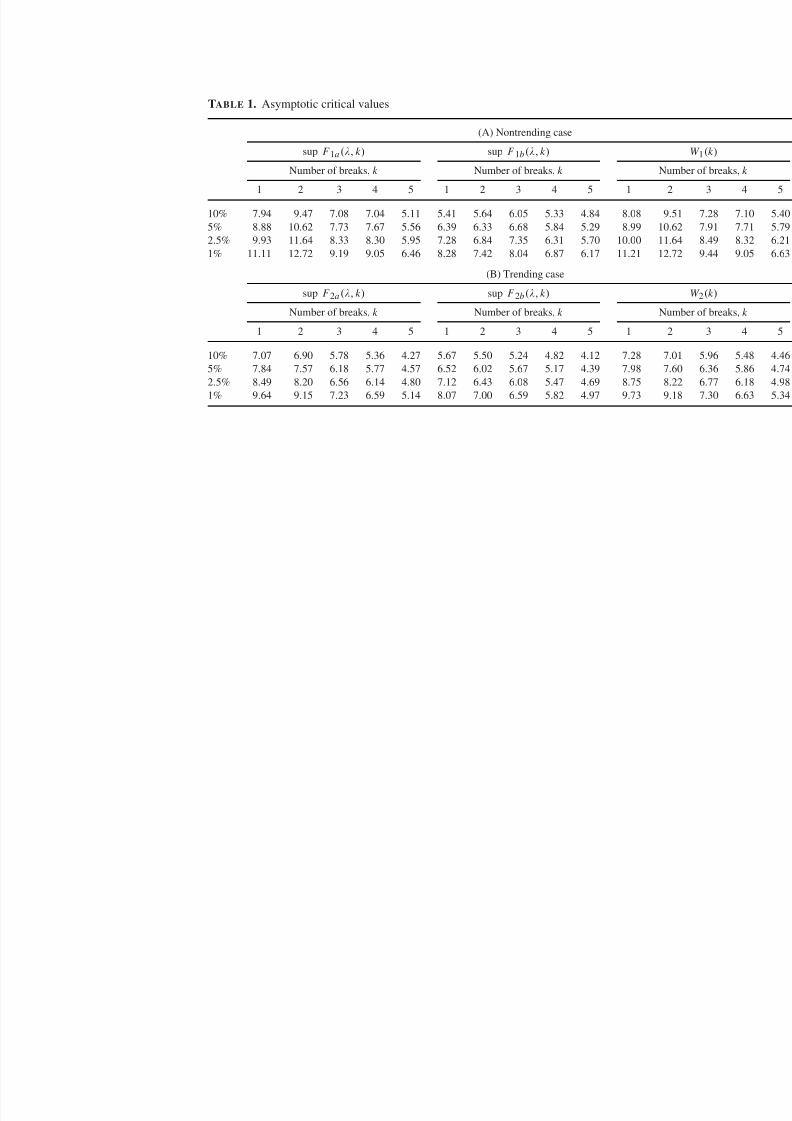
Asymptotic critical values are provided in Table 1 with the level of trimming
set at = 0.15. The maximum number of breaks considered is 5. Panel A pro-vides critical values for the nontrending case, while those for the trending case
are presented in Panel B. The critical values for Models 1a and 2a are larger than
those for Models 1b and 2b, respectively. Note also that the critical values are
not monotonically decreasing as k increases. This is due to the fact that the limit
7/25/2019 WALD TESTS FOR DETECTING MULTIPLE STRUCTURAL CHANGES IN PERSISTENCE
http://slidepdf.com/reader/full/wald-tests-for-detecting-multiple-structural-changes-in-persistence 10/35
TABLE 1. Asymptotic critical values
(A) Nontrending case
sup F 1a (λ, k ) sup F 1b(λ, k )
Number of breaks, k Number of breaks, k
1 2 3 4 5 1 2 3 4 5 1
10% 7.94 9.47 7.08 7.04 5.11 5.41 5.64 6.05 5.33 4.84 8.08
5% 8.88 10.62 7.73 7.67 5.56 6.39 6.33 6.68 5.84 5.29 8.99
2.5% 9.93 11.64 8.33 8.30 5.95 7.28 6.84 7.35 6.31 5.70 10.00
1% 11.11 12.72 9.19 9.05 6.46 8.28 7.42 8.04 6.87 6.17 11.21
(B) Trending case
sup F 2a (λ, k ) sup F 2b(λ, k )
Number of breaks, k Number of breaks, k
1 2 3 4 5 1 2 3 4 5 1
10% 7.07 6.90 5.78 5.36 4.27 5.67 5.50 5.24 4.82 4.12 7.28
5% 7.84 7.57 6.18 5.77 4.57 6.52 6.02 5.67 5.17 4.39 7.98
2.5% 8.49 8.20 6.56 6.14 4.80 7.12 6.43 6.08 5.47 4.69 8.75
1% 9.64 9.15 7.23 6.59 5.14 8.07 7.00 6.59 5.82 4.97 9.73
7/25/2019 WALD TESTS FOR DETECTING MULTIPLE STRUCTURAL CHANGES IN PERSISTENCE
http://slidepdf.com/reader/full/wald-tests-for-detecting-multiple-structural-changes-in-persistence 11/35
DETECTING MULTIPLE CHANGES IN PERSISTENCE 11
distributions are different for the cases with k even or odd. For even or odd values
they are, in general, monotonically decreasing as expected.
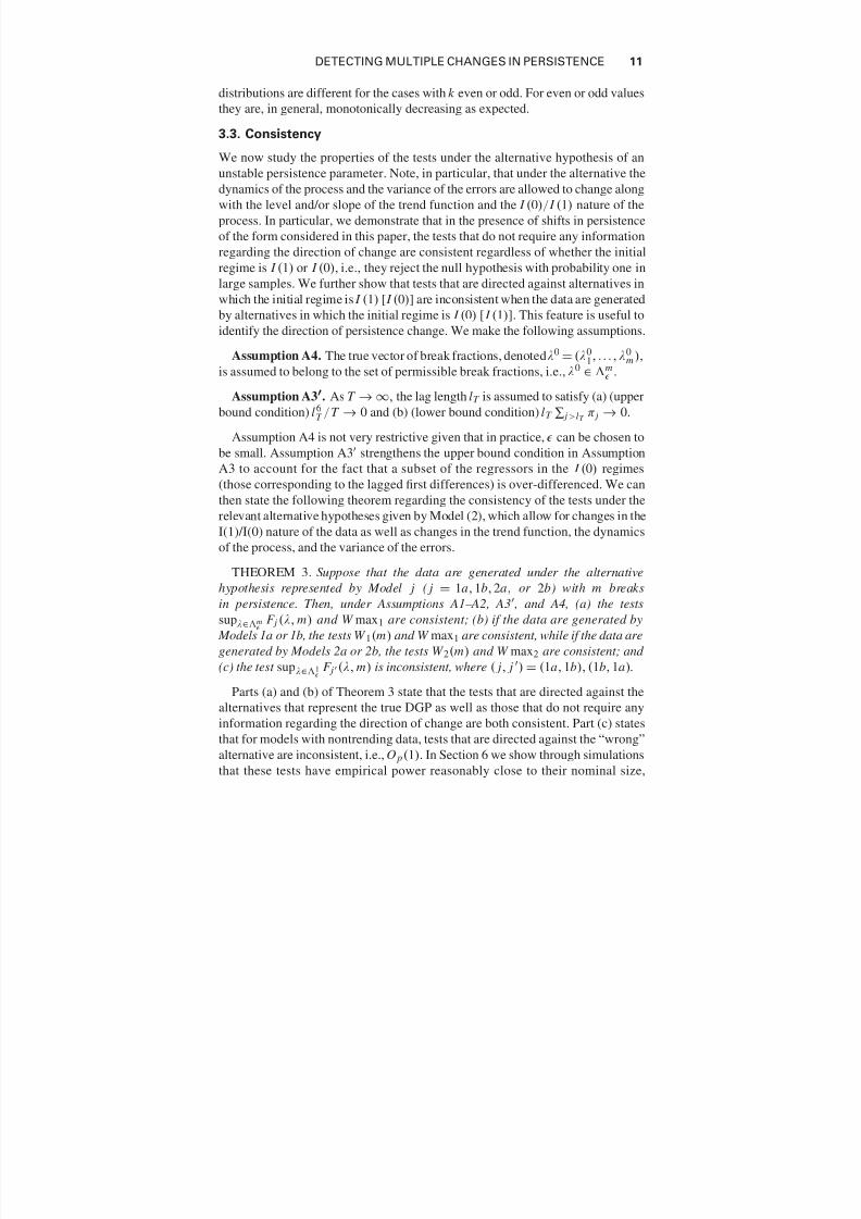
3.3. Consistency
We now study the properties of the tests under the alternative hypothesis of an
unstable persistence parameter. Note, in particular, that under the alternative the
dynamics of the process and the variance of the errors are allowed to change along
with the level and/or slope of the trend function and the I (0)/ I (1) nature of the
process. In particular, we demonstrate that in the presence of shifts in persistence
of the form considered in this paper, the tests that do not require any information
regarding the direction of change are consistent regardless of whether the initial
regime is I (1) or I (0), i.e., they reject the null hypothesis with probability one in
large samples. We further show that tests that are directed against alternatives inwhich the initial regime is I (1) [ I (0)] are inconsistent when the data are generated
by alternatives in which the initial regime is I (0) [ I (1)]. This feature is useful to
identify the direction of persistence change. We make the following assumptions.
Assumption A4. The true vector of break fractions, denoted λ0 = (λ01, . . . , λ0
m ),
is assumed to belong to the set of permissible break fractions, i.e., λ0 ∈ m .
Assumption A3. As T → ∞, the lag length lT is assumed to satisfy (a) (upper
bound condition) l 6T /T → 0 and (b) (lower bound condition) lT ∑ j >lT
π j → 0.
Assumption A4 is not very restrictive given that in practice, can be chosen to
be small. Assumption A3 strengthens the upper bound condition in Assumption
A3 to account for the fact that a subset of the regressors in the I (0) regimes
(those corresponding to the lagged first differences) is over-differenced. We can
then state the following theorem regarding the consistency of the tests under the
relevant alternative hypotheses given by Model (2), which allow for changes in the
I(1)/I(0) nature of the data as well as changes in the trend function, the dynamics
of the process, and the variance of the errors.
THEOREM 3. Suppose that the data are generated under the alternative
hypothesis represented by Model j ( j = 1a, 1b, 2a, or 2b) with m breaks
in persistence. Then, under Assumptions A1–A2, A3 , and A4, (a) the tests
supλ∈m
F j (λ, m) and W max1 are consistent; (b) if the data are generated by
Models 1a or 1b, the tests W 1(m) and W max1 are consistent, while if the data are
generated by Models 2a or 2b, the tests W 2(m) and W max2 are consistent; and
(c) the test supλ∈1
F j (λ, m) is inconsistent, where ( j, j ) = (1a, 1b), (1b, 1a).
Parts (a) and (b) of Theorem 3 state that the tests that are directed against the
alternatives that represent the true DGP as well as those that do not require anyinformation regarding the direction of change are both consistent. Part (c) states
that for models with nontrending data, tests that are directed against the “wrong”
alternative are inconsistent, i.e., O p(1). In Section 6 we show through simulations
that these tests have empirical power reasonably close to their nominal size,
7/25/2019 WALD TESTS FOR DETECTING MULTIPLE STRUCTURAL CHANGES IN PERSISTENCE
http://slidepdf.com/reader/full/wald-tests-for-detecting-multiple-structural-changes-in-persistence 12/35
12 MOHITOSH KEJRIWAL ET AL.
thereby enabling the applied researcher to infer the direction of shift from the test
outcomes.
4. HYBRID TESTING PROCEDURES
One aspect of the test statistics introduced in Section 2 is that they will reject the
null with probability one in large samples even if the process is stable I (0) or
one that involves changes in the value of the autoregressive parameter such that
the process is still I (0) in each regime, i.e., I (0) preserving changes. In practice,
the researcher may be interested in reliably interpreting the test outcome as one
emanating from a switch between an I (1) and an I (0) regime. To accommodate
such an interpretation, we propose hybrid testing procedures that entail the joint
application of our tests with the Bai and Perron (1998) structural change testsdesigned for a stationary framework as well as the unit root tests proposed by Ng
and Perron (2001) with the modification of Perron and Qu (2007) to select the lag
length. The number of breaks m is assumed to be known.
The first hybrid procedure is designed to test the null hypothesis that the pro-
cess is stable I (1) or stable I (0). To this end, we define B P(m) as the Bai-Perron
(1998) partial structural change test that jointly tests the stability of the intercept
and the autoregressive parameter in (4) while holding fixed the coefficients on the
lagged first differences. This test has the correct asymptotic size when the pro-
cess is constant I (0). We therefore employ the following decision rule labeledthe Dm test: “Reject the null if both W 1(m) and B P(m) reject.” If the signifi-
cance level κ is employed for both tests, the asymptotic size of Dm cannot exceed
κ, regardless of whether the process is I (1) or I (0) throughout. Further, since
B P(m) and W 1(m) are both consistent against processes that involve a switch
between an I (1) and an I (0) regime, Dm has unit asymptotic power against such
alternatives. Here, the assumption of a known number of breaks can be relaxed
using the W max1 test and the UDmax version of the BP test.
The second hybrid procedure allows the null hypothesis to include the case of
I (0) preserving changes in addition to the stable I (1)/ I (0) cases. This procedureis useful if the researcher seeks to distinguish between I (0) preserving changes
and those that involve at least one switch between an I (1) and an I (0) regime.
To facilitate this distinction, we note that with I (0) preserving changes, a unit
root test applied on the regime with the largest estimated autoregressive root will
reject the null asymptotically, while if an I (1) segment is present, such a test will
reject only with probability equal to the nominal significance level in large sam-
ples. We therefore recommend using the Dm procedure in conjunction with one
of the M G L S tests proposed by Ng and Perron (2001) with the modification of
Perron and Qu (2007) to select the lag length, given that these tests avoid thepower reversal problem for nonlocal stationary alternatives while maintaining
empirical size close to nominal size. The former feature ensures that our hybrid
procedure is well sized, while the latter ensures little loss in power. We therefore
propose joint application of the Dm procedure and the particular M G L S test on
7/25/2019 WALD TESTS FOR DETECTING MULTIPLE STRUCTURAL CHANGES IN PERSISTENCE
http://slidepdf.com/reader/full/wald-tests-for-detecting-multiple-structural-changes-in-persistence 13/35
DETECTING MULTIPLE CHANGES IN PERSISTENCE 13
the regime with the largest estimated autoregressive root, where the regimes are
identified by minimizing the unrestricted sum of squared residuals. Specifically,
the decision rule, labeled the J m test is: “Reject the null if Dm rejects and M G L S
does not reject.” If a significance level κ is used for each of the tests in Dm aswell as for M G L S , the asymptotic size of J m is bounded by κ, while for persis-
tence changes that involve switches between I (1) and I (0) regimes, its asymp-
totic power is (1 − κ). The finite sample performance of Dm and J m will be in-
vestigated through simulations in Section 6. Using the J m test, in large samples
one can obtain a complete correct classification into I (0) or I (1) throughout,
I (0) changes or I (1)/ I (0) changes by letting the size of each test go to zero at a
suitable rate.
5. ESTIMATORS FOR THE BREAK DATES
Following evidence against the null hypothesis, it is desirable to determine the
location of the break dates. To this end, we propose estimating the break date
estimators from global minimization of the sum of squared residuals under
the relevant alternative hypothesis. For a model with k breaks, the estimated
break dates are thus obtained as (T 1, . . . , T k ) = argminT 1,...,T k S S R j,k (T 1, . . . , T k )
where S S R j,k (T 1, . . . , T k ) is the sum of squared residuals for Model j ( j =
1a, 1b, 2a, 2b) evaluated at the partition {T 1, . . . , T k }.1 When estimating the break
dates, we allow the coefficients on the lagged first differences to vary acrossregimes. The number of lags is also allowed to be regime dependent. The com-
putation of the sum of squared residuals is similar to that discussed in Section 2
except that the cross-regime restrictions on the coefficients governing the short-
run dynamics are replaced by within-regime restrictions depending on the number
of lags included in a specific regime. The asymptotic properties of these estima-
tors, including their consistency, rate of convergence, and limit distribution, are
investigated in a companion paper (Kejriwal and Perron, 2012). Simulations (not
reported here) show that the estimators perform very well in small samples in
terms of bias and root mean squared error.
6. SIMULATION EXPERIMENTS
In this section we conduct simulation experiments to assess the finite sample
performance of the proposed tests as well as to provide a comparison with the
tests proposed in Harvey et al. (2006) and Leybourne et al. (2007b). We report
results only for the nontrending case, given that qualitatively similar results
were obtained for the trending case. In particular, we consider the statistics
W 1(1), W 1(2), D1, D2, J 1, and J 2. Results for the W max1 test were found to besimilar to those for the W 1 test based on the true number of breaks and hence
not reported. The Harvey et al. class of tests is designed to detect a single persis-
tence break and is based on partial sums of the demeaned or detrended data. They
recommend using the so-called “m min-modified” and “Sm min-modified” tests
7/25/2019 WALD TESTS FOR DETECTING MULTIPLE STRUCTURAL CHANGES IN PERSISTENCE
http://slidepdf.com/reader/full/wald-tests-for-detecting-multiple-structural-changes-in-persistence 14/35
14 MOHITOSH KEJRIWAL ET AL.
based on extensive simulation experiments. These tests differ in the method used
to compute the critical values. Given their similar finite sample performance, we
only report results for the “m min-modified” tests. Further, we present results only
for the test based on the mean-functional, denoted H , since this was found to out-perform the maximum and exponential versions in most of our experiments (as in
Harvey et al.) while producing very similar results in others. The Leybourne et al.
(2007b) tests allows for multiple changes and are based on a doubly recursive
application of the unit root statistic using the local GLS detrending methodology
developed in Elliott et al. (1996). More specifically, they propose the test statistic
M = inf λ∈(0,1) inf τ ∈(λ,1] D F G (λ,τ), where D F G (λ,τ) is the local GLS detrended
ADF unit root t -statistic that uses the observations between λT and τ T . Both the
H and M tests allow the process to be stable I (1) or stable I (0) under the null
hypothesis.We consider cases where the data generating processes (DGPs) involve no
break (size), as well as some involving one and two breaks (power). The sam-
ple sizes used are T = 150, 240. The lag length in the autoregression for our
proposed procedures is selected using the Bayesian information criterion (BIC)
with the maximum number of lags allowed set at 10. We first obtain the number
of lags based on the estimation of the alternative model and then use this num-
ber in the estimation of the null model. For the M test we used the Gauss posted
by Leybourne et al. (2007b) posted on the Studies in Nonlinear Dynamics and
Econometrics website, so that the lag length selection is based on the sequentialapproach of Ng and Perron (1995), with a maximal lag order of four and a 10%
significance level for the t -test on the highest lag. In order to account for the sta-
ble I (0) possibility under the null, the rejection frequency of the M -procedure
is computed as the proportion of Monte Carlo replications in which the M test
rejects, and the corresponding partition selected by the test does not correspond
to the full sample. Finally, to compute J m , we use the M Z G L S α unit root test of Ng
and Perron (2001) with the modification of Perron and Qu (2007) to select the lag
length with a maximum of five lags.2
In all experiments, {et } denotes a sequence of i.i.d. N (0, 1) variables. The errors{ut } are generated by the autoregressive moving average (ARMA) process ut =
ρut −1 + et + θ et −1, u0 = 0. We present results for the following combinations
of values of the autoregressive parameter (ρ ) and the moving average parameter
(θ ): (a) ρ = θ = 0; (b) ρ = 0.5, θ = 0; (c) ρ = 0, θ = 0.5; (d) ρ = 0, θ = −0.5;
(e) ρ = 0.3, θ = 0.5; (f) ρ = 0.3, θ = −0.5. The nominal size for all tests is set
at 5%. All experiments are based on 1, 000 replications.
6.1. The Empirical Size of the Tests
In order to assess the empirical size of the tests, the DGP considered is DGP-0:
yt = α yt −1 + ut , y0 = 0. The results are presented in Table 2a for α = 1 and
Table 2b for α < 1. For the latter, we report results only for ρ = θ = 0, although
the full set of results is available upon request. Consider first the unit root case.
7/25/2019 WALD TESTS FOR DETECTING MULTIPLE STRUCTURAL CHANGES IN PERSISTENCE
http://slidepdf.com/reader/full/wald-tests-for-detecting-multiple-structural-changes-in-persistence 15/35
DETECTING MULTIPLE CHANGES IN PERSISTENCE 15
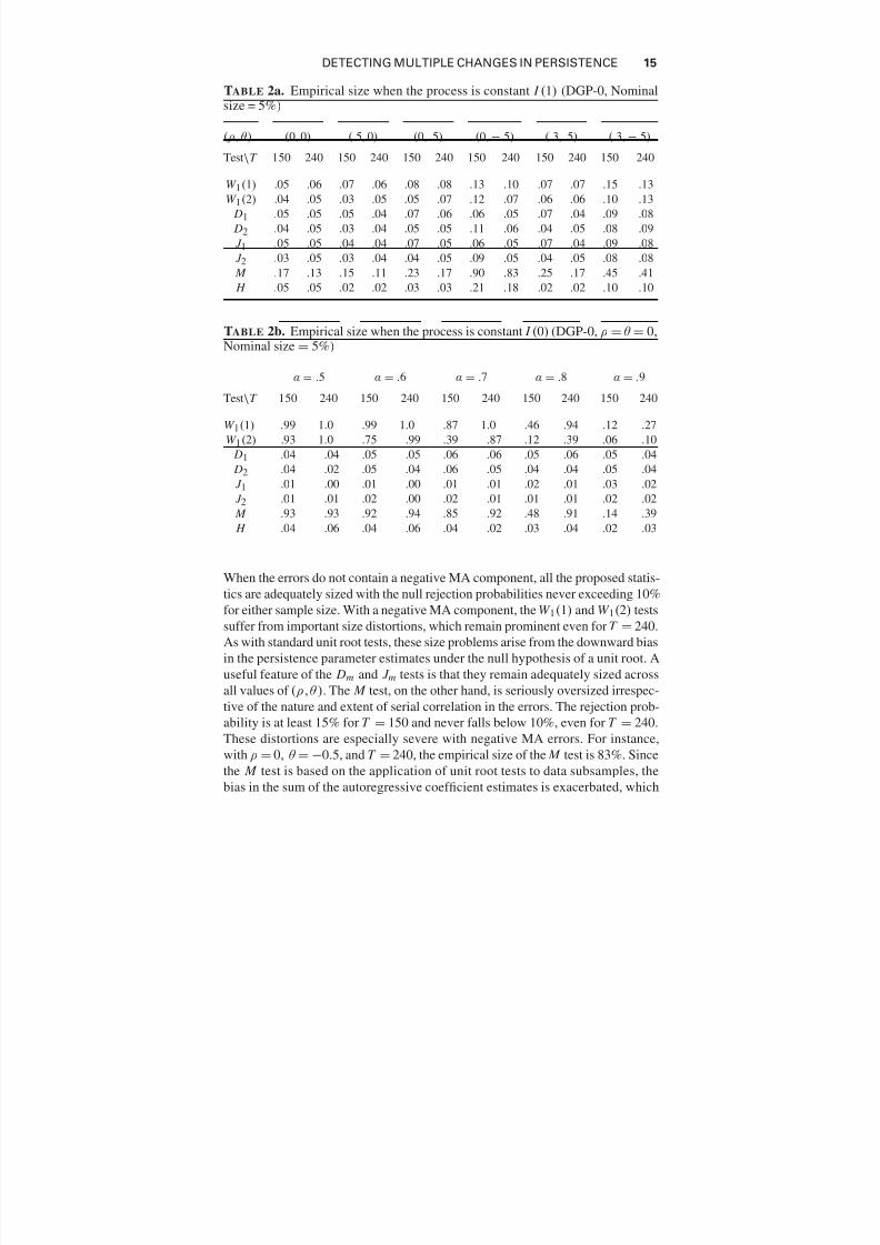
TABLE 2a. Empirical size when the process is constant I (1) (DGP-0, Nominalsize = 5%)
(ρ, θ ) (0, 0) (.5, 0) (0, .5) (0, −.5) (.3, .5) (.3, −.5)
Test\T 150 240 150 240 150 240 150 240 150 240 150 240
W 1(1) .05 .06 .07 .06 .08 .08 .13 .10 .07 .07 .15 .13
W 1(2) .04 .05 .03 .05 .05 .07 .12 .07 .06 .06 .10 .13
D1 .05 .05 .05 .04 .07 .06 .06 .05 .07 .04 .09 .08
D2 .04 .05 .03 .04 .05 .05 .11 .06 .04 .05 .08 .09
J 1 .05 .05 .04 .04 .07 .05 .06 .05 .07 .04 .09 .08
J 2 .03 .05 .03 .04 .04 .05 .09 .05 .04 .05 .08 .08
M .17 .13 .15 .11 .23 .17 .90 .83 .25 .17 .45 .41
H .05 .05 .02 .02 .03 .03 .21 .18 .02 .02 .10 .10
TABLE 2b. Empirical size when the process is constant I (0) (DGP-0, ρ = θ = 0,Nominal size = 5%)
α = .5 α = .6 α = .7 α = .8 α = .9
Test\T 150 240 150 240 150 240 150 240 150 240
W 1(1) .99 1.0 .99 1.0 .87 1.0 .46 .94 .12 .27
W 1(2) .93 1.0 .75 .99 .39 .87 .12 .39 .06 .10
D1 .04 .04 .05 .05 .06 .06 .05 .06 .05 .04
D2 .04 .02 .05 .04 .06 .05 .04 .04 .05 .04
J 1 .01 .00 .01 .00 .01 .01 .02 .01 .03 .02
J 2 .01 .01 .02 .00 .02 .01 .01 .01 .02 .02
M .93 .93 .92 .94 .85 .92 .48 .91 .14 .39
H .04 .06 .04 .06 .04 .02 .03 .04 .02 .03
When the errors do not contain a negative MA component, all the proposed statis-tics are adequately sized with the null rejection probabilities never exceeding 10%
for either sample size. With a negative MA component, the W 1(1) and W 1(2) tests
suffer from important size distortions, which remain prominent even for T = 240.
As with standard unit root tests, these size problems arise from the downward bias
in the persistence parameter estimates under the null hypothesis of a unit root. A
useful feature of the Dm and J m tests is that they remain adequately sized across
all values of (ρ,θ ). The M test, on the other hand, is seriously oversized irrespec-
tive of the nature and extent of serial correlation in the errors. The rejection prob-
ability is at least 15% for T = 150 and never falls below 10%, even for T = 240.These distortions are especially severe with negative MA errors. For instance,
with ρ = 0, θ = −0.5, and T = 240, the empirical size of the M test is 83%. Since
the M test is based on the application of unit root tests to data subsamples, the
bias in the sum of the autoregressive coefficient estimates is exacerbated, which
7/25/2019 WALD TESTS FOR DETECTING MULTIPLE STRUCTURAL CHANGES IN PERSISTENCE
http://slidepdf.com/reader/full/wald-tests-for-detecting-multiple-structural-changes-in-persistence 16/35
16 MOHITOSH KEJRIWAL ET AL.
in turn contributes to the poor finite sample performance of the test under the
null hypothesis. The H test is accurate except when a negative MA component
is present. When α < 1, the W 1(1), W 1(2), and M tests all overreject the null
substantially. These spurious rejections decline as α increases but remain nonneg-ligible for α ≤ 0.8. In contrast, the H , Dm , and J m tests maintain empirical size
very close to nominal size for all stationary values of α and both sample sizes.
6.2. The Case with One Break
We now consider the power of the tests with a single break and the following
DGPs:
For t ≤ [T λ01] For t ≥ [T λ0
1] + 1
DGP-1 yt = y t −1+ut yt = α yt −1+ut
DGP-2 yt = α yt −1+ut yt = y t −1+ut
DGP-3 yt = y t −1+π 1 yt −1+et yt = α yt −1+π 2 yt −1+et
DGP-4 yt = α yt −1+π 1 yt −1+et yt = y t −1+π 2 yt −1+et
DGP-5 yt = y t −1+ut yt − y[T λ01]= α( yt −1− y[T λ0
1]) + ut
DGP-1 and DGP-2 are processes involving a shift in the persistence parameter
but no change in the short-run dynamics. DGP-3 and DGP-4 allow for the short-
run dynamics to simultaneously change as well. We also examine the power of the
tests when the persistence parameter is unity but the short-run dynamics changeacross regimes, i.e., the data are generated by DGP-3 (or DGP-4) with α = 1 but
π1 = π2. DGP-5 is a variant of DGP-1 that is considered in Leybourne et al.
(2007b). Such a process is designed to avoid sharp jumps to zero at the break point
between the I (1) and I (0) regimes and ensures a joining up of these regimes. We
consider three values for the location of the break: λ01 = 0.3, 0.5, 0.7. We present
results for three values of the autoregressive parameter: α = 0.5, 0.7, 0.8. Given
the extent of size distortions, the powers of W 1(1), W 1(2), and M tests are all size-
adjusted. The results are presented in Table 3. We only report results for λ01 = 0.5
and T = 240 (more results are available in the working paper version, includingthose for T = 150). Power does vary with the location of the break: As expected,
it is higher when the break occurs early (λ01 = 0.3) and lower when it occurs late
(λ01 = 0.7) for DGP-1,3,5 and vice versa for DGP-2,4. This is due to the fact
that the longer the I (0) segment, the further away the series is from a pure unit
root process. Relative to the H test and the proposed tests, however, the M test
is much more sensitive to break location. Otherwise, the qualitative features are
similar.3
Panel (A) of Table 3 provides results for DGP-1. As expected, the power of
all the tests decreases as α increases. Power is also lower with serially corre-lated errors compared to the i.i.d. case, except when the errors contain a negative
MA component. The tests are thus subject to a clear size-power trade-off in this
latter case. The loss in power from introducing an autoregressive component in
the errors is especially significant for the M test, e.g., power falls from 79% to

7/25/2019 WALD TESTS FOR DETECTING MULTIPLE STRUCTURAL CHANGES IN PERSISTENCE
http://slidepdf.com/reader/full/wald-tests-for-detecting-multiple-structural-changes-in-persistence 17/35
DETECTING MULTIPLE CHANGES IN PERSISTENCE 17
TABLE 3. Empirical power with one break (λ01 = 0.5); T = 240
α = 0.5 α = 0.7 α = 0.8
W 1 D1 J 1 M H W 1 D1 J 1 M H W 1 D1 J 1 M H
(ρ,θ) (A) DGP-1
(0, 0) 1.0 1.0 .97 1.0 .93 .99 .94 .90 .79 .70 .84 .79 .76 .37 .38
(.5, 0) 1.0 1.0 .95 .79 .81 .95 .93 .88 .45 .48 .76 .76 .73 .26 .21
(0, .5) 1.0 1.0 .95 .92 .90 .95 .91 .87 .55 .62 .74 .74 .72 .29 .30
(0, −.5) .99 .99 .92 .99 . 97 .93 .91 .85 .87 .87 .78 .76 .73 .48 .66
(.3, .5) 1.0 .99 .99 .79 .85 .94 .91 .91 .47 .52 .73 .72 .72 .26 .24
(.3, −.5) 1.0 1.0 .95 1.0 .96 .97 .95 .86 .88 .81 .83 .83 .69 .47 .52
(ρ, θ ) (B) DGP-2
(0, 0) 1.0 .99 .95 1.0 .96 .82 .75 .72 .88 .82 .37 .30 .28 .50 .60
(.5, 0) .93 .93 .89 .85 . 90 .52 .54 .51 .57 .68 .24 .23 .20 .34 .43
(0, .5) .95 .96 .92 .94 . 94 .60 .60 .57 .67 .76 .30 .29 .26 .39 .54
(0, −.5) .93 .94 .88 1.0 .98 .76 .77 .73 .90 .90 .48 .54 .50 .55 .78
(.3, .5) .91 .91 .87 .84 .92 .50 .50 .46 .55 .71 .24 .22 .18 .35 .47
(.3, −.5) .98 .99 .93 1.0 .98 .85 .88 .83 .91 .86 .57 .65 .60 .59 .69
(π1, π2) (C) DGP-3
(0. −.2) 1.0 1.0 .96 .94 . 94 .99 .98 .91 .73 .66 .90 .86 .80 .51 .37
(−.3, − .5) 1.0 1.0 .96 .79 .91 .97 .95 .90 .48 .61 .78 .76 .70 .35 .35
(π1, π2) (D) DGP-4
(0. −.2) .91 .90 .89 1.0 .95 .54 .53 .64 .90 .77 .31 .31 .26 .57 .55
(−.3, −.5) .74 .71 .68 .79 .93 .21 .20 .21 .45 .69 .09 .07 .06 .26 .48
(ρ,θ) (E) DGP-5
(0, 0) 1.0 1.0 .94 1.0 .96 .98 .93 .87 .91 .84 .81 .71 .67 .53 .59
(.5, 0) 1.0 .99 .93 .88 . 91 .91 .85 .78 .59 .70 .66 .63 .59 .36 .42
(0, .5) 1.0 1.0 .93 .94 . 95 .89 .85 .78 .70 .79 .65 .61 .58 .41 .53
(0, −.5) .98 .98 .89 1.0 .98 .89 .91 .83 .92 .91 .74 .71 .65 .60 .78
(.3, .5) .99 .99 .92 .85 .93 .87 .78 .74 .58 .73 .61 .56 .52 .35 .46
(.3, −.5) 1.0 1.0 .92 1.0 .97 .94 .94 .85 .95 .89 .79 .78 .71 .64 .68
Note: In all cases, W 1 stands for the statistic W 1(1).
45% as ρ increases from 0 to 0.5 when α = 0.7. In comparison, the power of theproposed tests is much more robust to the extent of error serial correlation. More-
over, there is only a mild loss in power from using the D1 and J 1 tests compared
to the less robust W 1(1). This property is important in applications where the re-
searcher does not want to take a stand on the nature of the process under the null
7/25/2019 WALD TESTS FOR DETECTING MULTIPLE STRUCTURAL CHANGES IN PERSISTENCE
http://slidepdf.com/reader/full/wald-tests-for-detecting-multiple-structural-changes-in-persistence 18/35
18 MOHITOSH KEJRIWAL ET AL.
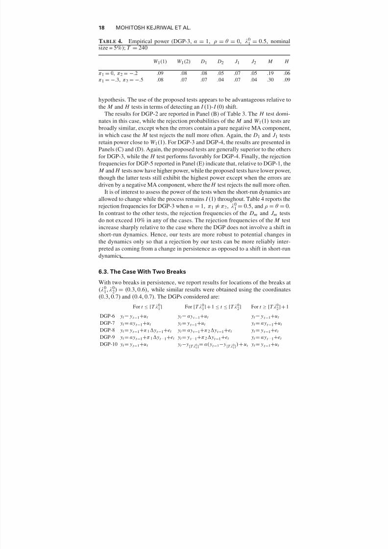
TABLE 4. Empirical power (DGP-3, α = 1, ρ = θ = 0, λ01 = 0.5, nominal
size = 5%); T = 240
W 1(1) W 1(2) D1 D2 J 1 J 2 M H
π1 = 0, π2 = −.2 .09 .08 .08 .05 .07 .05 .19 .06
π1 = −.3, π2 = −.5 .08 .07 .07 .04 .07 .04 .30 .09
hypothesis. The use of the proposed tests appears to be advantageous relative to
the M and H tests in terms of detecting an I (1)- I (0) shift.
The results for DGP-2 are reported in Panel (B) of Table 3. The H test domi-
nates in this case, while the rejection probabilities of the M and W 1(1) tests are
broadly similar, except when the errors contain a pure negative MA component,in which case the M test rejects the null more often. Again, the D1 and J 1 tests
retain power close to W 1(1). For DGP-3 and DGP-4, the results are presented in
Panels (C) and (D). Again, the proposed tests are generally superior to the others
for DGP-3, while the H test performs favorably for DGP-4. Finally, the rejection
frequencies for DGP-5 reported in Panel (E) indicate that, relative to DGP-1, the
M and H tests now have higher power, while the proposed tests have lower power,
though the latter tests still exhibit the highest power except when the errors are
driven by a negative MA component, where the H test rejects the null more often.
It is of interest to assess the power of the tests when the short-run dynamics areallowed to change while the process remains I (1) throughout. Table 4 reports the
rejection frequencies for DGP-3 when α = 1, π1 = π2, λ01 = 0.5, and ρ = θ = 0.
In contrast to the other tests, the rejection frequencies of the Dm and J m tests
do not exceed 10% in any of the cases. The rejection frequencies of the M test
increase sharply relative to the case where the DGP does not involve a shift in
short-run dynamics. Hence, our tests are more robust to potential changes in
the dynamics only so that a rejection by our tests can be more reliably inter-
preted as coming from a change in persistence as opposed to a shift in short-run
dynamics.
6.3. The Case With Two Breaks
With two breaks in persistence, we report results for locations of the breaks at
(λ01, λ0
2) = (0.3, 0.6), while similar results were obtained using the coordinates
(0.3, 0.7) and (0.4, 0.7). The DGPs considered are:
For t ≤ [T λ01] For [T λ0
1] + 1 ≤ t ≤ [T λ02] For t ≥ [T λ0
2] + 1
DGP-6 yt = y t −1+ut yt = α yt −1+ut yt = y t −1+ut
DGP-7 yt = α yt −1+ut yt = y t −1+ut yt = α yt −1+ut
DGP-8 yt = y t −1+π 1 yt −1+et yt = α yt −1+π 2 yt −1+et yt = y t −1+et
DGP-9 yt = α yt −1+π 1 yt −1+et yt = y t −1+π 2 yt −1+et yt = α yt −1+et
DGP-10 yt = y t −1+ut yt − y[T λ01]
= α( yt −1− y[T λ01]) + ut yt = y t −1+ut
7/25/2019 WALD TESTS FOR DETECTING MULTIPLE STRUCTURAL CHANGES IN PERSISTENCE
http://slidepdf.com/reader/full/wald-tests-for-detecting-multiple-structural-changes-in-persistence 19/35
DETECTING MULTIPLE CHANGES IN PERSISTENCE 19
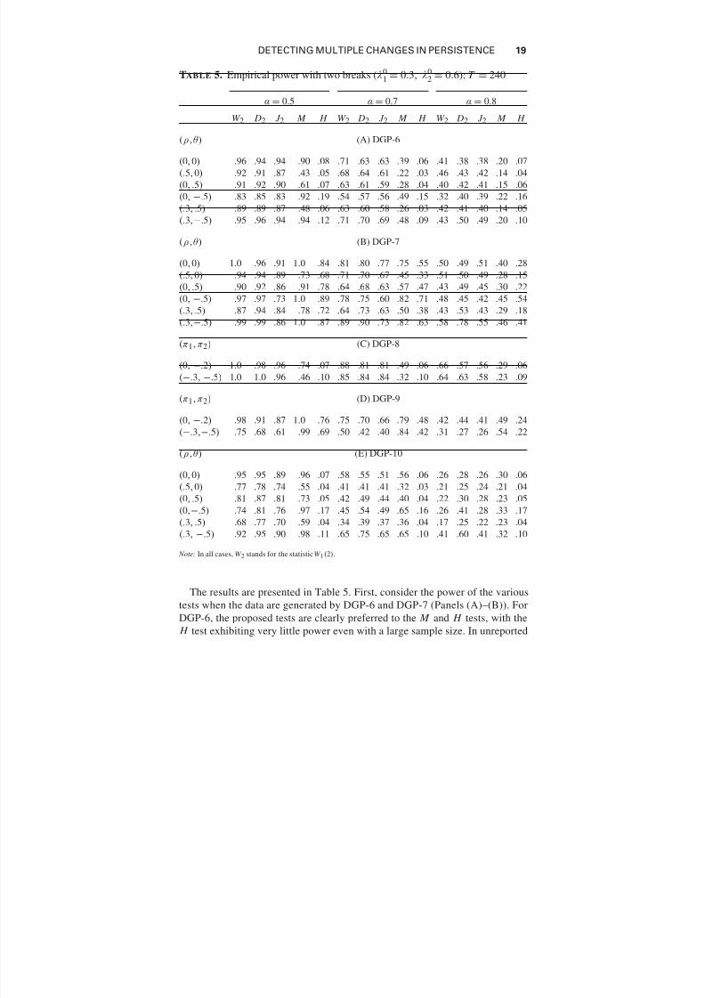
TABLE 5. Empirical power with two breaks (λ01 = 0.3, λ0
2 = 0.6); T = 240
α = 0.5 α = 0.7 α = 0.8
W 2 D2 J 2 M H W 2 D2 J 2 M H W 2 D2 J 2 M H
(ρ,θ) (A) DGP-6
(0, 0) .96 .94 .94 .90 .08 .71 .63 .63 .39 .06 .41 .38 .38 .20 .07
(.5, 0) .92 .91 .87 .43 .05 .68 .64 .61 .22 .03 .46 .43 .42 .14 .04
(0, .5) .91 .92 .90 .61 .07 .63 .61 .59 .28 .04 .40 .42 .41 .15 .06
(0, −.5) .83 .85 .83 .92 .19 .54 .57 .56 .49 .15 .32 .40 .39 .22 .16
(.3, .5) .89 .89 .87 .48 .06 .63 .60 .58 .26 .03 .42 .41 .40 .14 .05
(.3,−.5) .95 .96 .94 .94 .12 .71 .70 .69 .48 .09 .43 .50 .49 .20 .10
(ρ,θ) (B) DGP-7
(0, 0) 1.0 .96 .91 1.0 .84 .81 .80 .77 .75 .55 .50 .49 .51 .40 .28
(.5, 0) .94 .94 .89 .73 .68 .71 .70 .67 .45 .33 .51 .50 .49 .28 .15
(0, .5) .90 .92 .86 .91 .78 .64 .68 .63 .57 .47 .43 .49 .45 .30 .22
(0, −.5) .97 .97 .73 1.0 .89 .78 .75 .60 .82 .71 .48 .45 .42 .45 .54
(.3, .5) .87 .94 .84 .78 .72 .64 .73 .63 .50 .38 .43 .53 .43 .29 .18
(.3,−.5) .99 .99 .86 1.0 .87 .89 .90 .73 .82 .63 .58 .78 .55 .46 .41
(π1, π2) (C) DGP-8
(0, −.2) 1.0 .98 .96 .74 .07 .88 .81 .81 .49 .06 .66 .57 .56 .29 .06
(−.3, −.5) 1.0 1.0 .96 .46 .10 .85 .84 .84 .32 .10 .64 .63 .58 .23 .09
(π1, π2) (D) DGP-9
(0, −.2) .98 .91 .87 1.0 .76 .75 .70 .66 .79 .48 .42 .44 .41 .49 .24
(−.3,−.5) .75 .68 .61 .99 .69 .50 .42 .40 .84 .42 .31 .27 .26 .54 .22
(ρ,θ) (E) DGP-10
(0, 0) .95 .95 .89 .96 .07 .58 .55 .51 .56 .06 .26 .28 .26 .30 .06
(.5, 0) .77 .78 .74 .55 .04 .41 .41 .41 .32 .03 .21 .25 .24 .21 .04
(0, .5) .81 .87 .81 .73 .05 .42 .49 .44 .40 .04 .22 .30 .28 .23 .05
(0,−.5) .74 .81 .76 .97 .17 .45 .54 .49 .65 .16 .26 .41 .28 .33 .17
(.3, .5) .68 .77 .70 .59 .04 .34 .39 .37 .36 .04 .17 .25 .22 .23 .04
(.3, −.5) .92 .95 .90 .98 .11 .65 .75 .65 .65 .10 .41 .60 .41 .32 .10
Note: In all cases, W 2 stands for the statistic W 1(2).
The results are presented in Table 5. First, consider the power of the various
tests when the data are generated by DGP-6 and DGP-7 (Panels (A)–(B)). For
DGP-6, the proposed tests are clearly preferred to the M and H tests, with the
H test exhibiting very little power even with a large sample size. In unreported
7/25/2019 WALD TESTS FOR DETECTING MULTIPLE STRUCTURAL CHANGES IN PERSISTENCE
http://slidepdf.com/reader/full/wald-tests-for-detecting-multiple-structural-changes-in-persistence 20/35
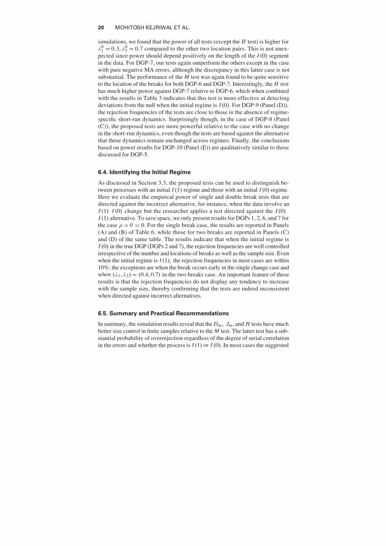
20 MOHITOSH KEJRIWAL ET AL.
simulations, we found that the power of all tests (except the H test) is higher for
λ01 = 0.3, λ0
2 = 0.7 compared to the other two location pairs. This is not unex-
pected since power should depend positively on the length of the I (0) segment
in the data. For DGP-7, our tests again outperform the others except in the casewith pure negative MA errors, although the discrepancy in this latter case is not
substantial. The performance of the M test was again found to be quite sensitive
to the location of the breaks for both DGP-6 and DGP-7. Interestingly, the H test
has much higher power against DGP-7 relative to DGP-6, which when combined
with the results in Table 3 indicates that this test is more effective at detecting
deviations from the null when the initial regime is I (0). For DGP-9 (Panel (D)),
the rejection frequencies of the tests are close to those in the absence of regime-
specific short-run dynamics. Surprisingly though, in the case of DGP-8 (Panel
(C)), the proposed tests are more powerful relative to the case with no changein the short-run dynamics, even though the tests are based against the alternative
that these dynamics remain unchanged across regimes. Finally, the conclusions
based on power results for DGP-10 (Panel (E)) are qualitatively similar to those
discussed for DGP-5.
6.4. Identifying the Initial Regime
As discussed in Section 3.3, the proposed tests can be used to distinguish be-
tween processes with an initial I (1) regime and those with an initial I (0) regime.Here we evaluate the empirical power of single and double break tests that are
directed against the incorrect alternative, for instance, when the data involve an
I (1)– I (0) change but the researcher applies a test directed against the I (0)–
I (1) alternative. To save space, we only present results for DGPs 1, 2, 6, and 7 for
the case ρ = θ = 0. For the single break case, the results are reported in Panels
(A) and (B) of Table 6, while those for two breaks are reported in Panels (C)
and (D) of the same table. The results indicate that when the initial regime is
I (0) in the true DGP (DGPs 2 and 7), the rejection frequencies are well controlled
irrespective of the number and locations of breaks as well as the sample size. Evenwhen the initial regime is I (1), the rejection frequencies in most cases are within
10%; the exceptions are when the break occurs early in the single change case and
when (λ1, λ2) = (0.4, 0.7) in the two breaks case. An important feature of these
results is that the rejection frequencies do not display any tendency to increase
with the sample size, thereby confirming that the tests are indeed inconsistent
when directed against incorrect alternatives.
6.5. Summary and Practical Recommendations
In summary, the simulation results reveal that the Dm , J m , and H tests have much
better size control in finite samples relative to the M test. The latter test has a sub-
stantial probability of overrejection regardless of the degree of serial correlation
in the errors and whether the process is I (1) or I (0). In most cases the suggested
7/25/2019 WALD TESTS FOR DETECTING MULTIPLE STRUCTURAL CHANGES IN PERSISTENCE
http://slidepdf.com/reader/full/wald-tests-for-detecting-multiple-structural-changes-in-persistence 21/35
DETECTING MULTIPLE CHANGES IN PERSISTENCE 21
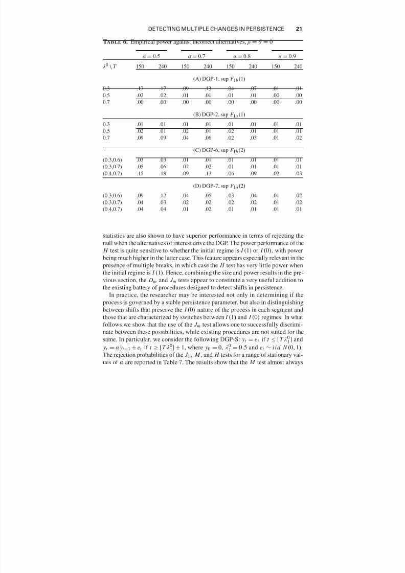
TABLE 6. Empirical power against incorrect alternatives, ρ = θ = 0
α = 0.5 α = 0.7 α = 0.8 α = 0.9
λ0 \ T 150 240 150 240 150 240 150 240
(A) DGP-1, sup F 1b(1)
0.3 .17 .17 .09 .13 .04 .07 .01 .01
0.5 .02 .02 .01 .01 .01 .01 .00 .00
0.7 .00 .00 .00 .00 .00 .00 .00 .00
(B) DGP-2, sup F 1a (1)
0.3 .01 .01 .01 .01 .01 .01 .01 .01
0.5 .02 .01 .02 .01 .02 .01 .01 .010.7 .09 .09 .04 .06 .02 .03 .01 .02
(C) DGP-6, sup F 1b(2)
(0.3,0.6) .03 .03 .01 .01 .01 .01 .01 .01
(0.3,0.7) .05 .06 .02 .02 .01 .01 .01 .01
(0.4,0.7) .15 .18 .09 .13 .06 .09 .02 .03
(D) DGP-7, sup F 1a (2)
(0.3,0.6) .09 .12 .04 .05 .03 .04 .01 .02
(0.3,0.7) .04 .03 .02 .02 .02 .02 .01 .02
(0.4,0.7) .04 .04 .01 .02 .01 .01 .01 .01
statistics are also shown to have superior performance in terms of rejecting the
null when the alternatives of interest drive the DGP. The power performance of the
H test is quite sensitive to whether the initial regime is I (1) or I (0), with power
being much higher in the latter case. This feature appears especially relevant in the
presence of multiple breaks, in which case the H test has very little power whenthe initial regime is I (1). Hence, combining the size and power results in the pre-
vious section, the Dm and J m tests appear to constitute a very useful addition to
the existing battery of procedures designed to detect shifts in persistence.
In practice, the researcher may be interested not only in determining if the
process is governed by a stable persistence parameter, but also in distinguishing
between shifts that preserve the I (0) nature of the process in each segment and
those that are characterized by switches between I (1) and I (0) regimes. In what
follows we show that the use of the J m test allows one to successfully discrimi-
nate between these possibilities, while existing procedures are not suited for thesame. In particular, we consider the following DGP-S: yt = et if t ≤ [T λ0
1] and
yt = α yt −1 + et if t ≥ [T λ01] + 1, where y0 = 0, λ0
1 = 0.5 and et ∼ i i d N (0, 1).
The rejection probabilities of the J 1, M , and H tests for a range of stationary val-
ues of α are reported in Table 7. The results show that the M test almost always

7/25/2019 WALD TESTS FOR DETECTING MULTIPLE STRUCTURAL CHANGES IN PERSISTENCE
http://slidepdf.com/reader/full/wald-tests-for-detecting-multiple-structural-changes-in-persistence 22/35
22 MOHITOSH KEJRIWAL ET AL.
TABLE 7. Null rejection probabilities for an I (0)- I (0) change (DGP-S, α1 = 0,
α2 = α, ρ = θ = 0, λ01 = 0.5)
α = .5 α = .6 α = .7 α = .8 α = .9
Test \T 150 240 150 240 150 240 150 240 150 240
J 1 .06 .07 .15 .06 .15 .07 .21 .08 .55 .23
M .96 .97 .98 .99 .99 1.0 1.0 1.0 1.0 1.0
H .22 .24 .27 .35 .44 .51 .68 .75 .87 .95
rejects, regardless of the sample size and the break magnitude. The H and J 1 tests
are much more sensitive to the magnitude of the change, rejecting the null morefrequently as the break becomes larger. Among the latter two tests, however, the
J 1 test is much more immune to the value of α, the likelihood of rejection be-
ing substantial only when α = 0.9 and T = 150. This experiment thus clearly
illustrates the usefulness of the recommended tests in identifying the nature of
the persistence shifts responsible for instabilities in the process generating the
data.
It remains to discuss how to disentangle a rejection of the proposed statistics as
coming from a change in persistence and not only a change in the trend function.
In the trendless case where the process is I (0) with pure level shifts, the use of the J m tests again provides a reliable safeguard, since its rejection frequencies are
controlled owing to the fact that the unit root test on the regime with the largest
estimated autoregressive unit root rejects with probability one in large samples
(given the consistency of the estimated breakpoints). Consider next the case where
the process is I (0) with breaks in the slope of the trend function. Then, our tests
will have power but so would unit root tests allowing for a change in the trend
function; see Kim and Perron (2009). If there are changes both in persistence
and in the slope of the trend, then the latter would not reject (see Kim, 2000).
So our test can be used in conjunction with those of Kim and Perron to makesure that a change in persistence is indeed present and not only a change in the
trend function. Finally, consider the case in which the process is I (1) across two
segments but with a change in trend. The following procedure can be used to
distinguish such a process from a persistence change process. We first detrend the
data using a regression of the data on a time trend and a slope dummy (where
the break date is chosen by minimizing the sum of squared residuals). We then
apply our persistence change tests to the detrended data. The problem is that the
limits of the resulting statistics under the unit root null depend on the true trend
break date. But we can use the critical values corresponding to Models 2a or 2b(as the case may be) as a benchmark. If there is only a pure trend break, these tests
should not reject the null, while if there is an accompanying change in persistence,
one of the tests (for Model 2a or 2b) would reject. To examine the finite sample
performance of the detrended test statistics in the single break case, we consider

7/25/2019 WALD TESTS FOR DETECTING MULTIPLE STRUCTURAL CHANGES IN PERSISTENCE
http://slidepdf.com/reader/full/wald-tests-for-detecting-multiple-structural-changes-in-persistence 23/35
DETECTING MULTIPLE CHANGES IN PERSISTENCE 23
TABLE 8. Empirical size and power of W 1(1) and W 2(1) (DGP-T, µ0 = β 0 = 0,τ 0 = 0.5) (For J 1: β 1 = 0, µ1 = 5 and for W 2(1): µ1 = 0, β 1 = 0.5)
T = 150 T = 240 T = 150 T = 240 T = 150 T = 240
J 1 W 2 J 1 W 2 J 1 W 2 J 1 W 2 J 1 W 2 J 1 W 2
α1 = α2 = 1 .04 .09 .05 .08
λ01 = 0.3 λ0
1 = 0.5 λ01 = 0.7
α1 = 1, α2 = 0.5 .71 .66 .78 .68 .93 .95 .96 .99 .86 .39 .97 .45
α1 = 1, α2 = 0.7 .37 .45 .67 .52 .70 .72 .92 .92 .55 .27 .80 .30
α1 = 0.5, α2 = 1 .33 .53 .76 .82 .78 .85 .95 .97 .71 .95 .96 1.0
α1 = 0.7, α2 = 1 .11 .22 .32 .44 .28 .47 .78 .80 .23 .56 .72 .90
the following DGP-T:
yt = µ0 + µ1 I (t > [T τ 01 ]) + β 0t + β 1(t − [T τ 0
1 ]) I (t > [T τ 01 ]) + y∗
t ,
where y∗t = α1 y∗
t −1 + et if t ≤ [λ01T ] and y∗
t = α2 y∗t −1 + et if t ≥ [λ0
1T ] + 1 with
y∗0 = 0, et ∼ i id N (0, 1). Note that we allow τ 0
1 = λ01. In the simulations, we
fix τ 01 = 0.5 and set λ01 = 0.3, 0.5, 0.7. We consider the case of a pure level shift(µ0 = β 0 = β 1 = 0, µ1 = 5) in which case the test J 1 is employed, as well as the
case of a trend break (µ0 = µ1 = β 0 = 0, β 1 = 0.5) in which case the test W 2(1) is
employed. The results are reported in Table 8. Note that in both the pure level shift
and trend break cases, the size remains adequate, never exceeding 10%. Power is
generally highest when the trend break date coincides with the persistence break
date. An exception is the trend break case where the persistence change is from an
I (0) to an I (1) process: Here, power is highest when the the trend break precedes
the persistence break. In the general case, which allows for the possibility that the
number of trend beaks can be different from the number of persistence breaks, wecan potentially adopt the following procedure. In a first step, the number of trend
breaks can be estimated using the sequential procedure developed by Kejriwal and
Perron (2010) that is robust to whether the errors are I (1) or I (0). This estimate
can subsequently be used to detrend the data and apply the W max2 test in the
second step. While such a procedure is likely to be computationally intensive, it
has the advantage of being agnostic to the types of breaks. Investigation of the
asymptotic and finite sample properties of such a procedure is left as an important
avenue for future research.
7. CONCLUSION
This paper has presented issues related to testing for multiple structural changes
in the persistence of a univariate time series. In contrast to the existing literature,
7/25/2019 WALD TESTS FOR DETECTING MULTIPLE STRUCTURAL CHANGES IN PERSISTENCE
http://slidepdf.com/reader/full/wald-tests-for-detecting-multiple-structural-changes-in-persistence 24/35
24 MOHITOSH KEJRIWAL ET AL.
which has primarily focused on subsample unit root tests and tests based on partial
sums of residuals, we propose sup-Wald tests based on the difference between
the sum of squared residuals under the null hypothesis of a unit root and that
under the alternative hypothesis that the process displays changes in persistenceover the sample. Our simulation experiments demonstrate that these tests have
adequate finite sample properties. One important issue that we have not addressed
is how to select the number of breaks. Indeed, we have assumed that the number
of breaks is known a priori or less than some known upper bound. Bai and Perron
(1998) propose a sequential strategy based on repeated application of the single
break test in the context of stationary regression models. Such a strategy, however,
does not directly extend to our framework, given that the process is stationary in
only some regimes but has a unit root in others. Developing methods that would
allow the consistent estimation of the number of breaks in this framework is animportant avenue for future research. Finally, it is important to address the issue
of the estimation of the break dates and develop a method to form confidence
intervals. These and other issues are the object of ongoing research.
NOTES
1. Such an estimate was proposed by Chong (2001) for an AR(1) model with a single shift in
persistence, although his estimation procedure did not impose the unit root restriction in the relevant
regime.
2. The size and power properties using other versions of the M G L S test were very similar.
3. The full set of results is available upon request.
REFERENCES
Andrews, D.W.K. (1993) Tests for parameter instability and structural change with unknown change
point. Econometrica 61, 821–856.
Bai, J. & P. Perron (1998) Estimating and testing linear models with multiple structural changes.
Econometrica 66, 47–78.
Bai, J. & P. Perron (2003) Computation and analysis of multiple structural change models. Journal of
Applied Econometrics 18, 1–22.
Barsky, R.B. (1987) The Fisher hypothesis and the forecastibility and persistence of inflation. Journal
of Monetary Economics 19, 3–24.
Berk, K.N. (1974) Consistent autoregressive spectral estimates. Annals of Statistics 2, 489–502.
Burdekin, R.C.K. & P.L. Siklos (1999) Exchange rate regimes and shifts in inflation persistence: Does
nothing else matter. Journal of Money, Credit and Banking 31, 235–247.
Busetti, F. & A.M.R. Taylor (2004) Tests of stationarity against a change in persistence. Journal of
Econometrics 123, 33–66.
Chang, M.C. (1989) Testing for Overdifferencing. Ph.D. dissertation, North Carolina State University.
Chang, M.C. & D.A. Dickey (1994) Recognizing overdifferenced time series. Journal of Time Series
Analysis 15, 1–18.Chong, T.T.L. (2001) Structural change in AR(1) models. Econometric Theory 17, 87–155.
DeLong, J.B. & L.H. Summers (1988) How does macroeconomic policy affect output? Brookings
Papers on Economic Activity 2, 433–494.
Elliott, G., T.J. Rothenberg, & J.H. Stock (1996) Efficient tests for an autoregressive unit root.
Econometrica 64, 813–836.
7/25/2019 WALD TESTS FOR DETECTING MULTIPLE STRUCTURAL CHANGES IN PERSISTENCE
http://slidepdf.com/reader/full/wald-tests-for-detecting-multiple-structural-changes-in-persistence 25/35
DETECTING MULTIPLE CHANGES IN PERSISTENCE 25
Hakkio, C.S. & M. Rush (1991) Is the budget deficit too large? Economic Inquiry 29, 429–445.
Harvey, D.I., S.J. Leybourne, & A.M.R. Taylor (2006) Modified tests for a change in persistence.
Journal of Econometrics 134, 441–469.
Kang, K.H., C.J. Kim, & J. Morley (2009) Changes in U.S. inflation persistence. Studies in Nonlinear
Dynamics & Econometrics vol. 13(4), article 1.
Kejriwal, M. & P. Perron (2010) A sequential procedure to determine the number of breaks in trend
with an integrated or stationary noise component. Journal of Time Series Analysis 31, 305–328.
Kejriwal, M. & P. Perron (2012) Estimating a Structural Change in Persistence. Manuscript in prepa-
ration, Boston University.
Kim, D. & P. Perron (2009) Unit root tests allowing for a break in the trend function under both the
null and alternative hypotheses. Journal of Econometrics 148, 1–13.
Kim, J.Y. (2000) Detection of change in persistence of a linear time series. Journal of Econometrics
54, 159–178.
Kim, J.Y. (2003) Inference on segmented cointegration. Econometric Theory 19, 620–639.
Kurozumi, E. (2005) Detection of structural change in the long-run persistence in a univariate time
series. Oxford Bulletin of Economics and Statistics 67, 181–206.
Leybourne, S.J., T. Kim, V. Smith, & P. Newbold (2003) Tests for a change in persistence against the
null of difference-stationarity. Econometrics Journal 6, 291–311.
Leybourne, S.J., T. Kim, & A.M.R. Taylor (2007a) CUSUM of squares-based tests for a change in
persistence. Journal of Time Series Analysis 28, 408–433.
Leybourne, S.J., T. Kim, & A.M.R. Taylor (2007b) Detecting multiple changes in persistence. Studies
in Nonlinear Dynamics & Econometrics vol. 11(3), article 2.
Lutkepohl, H. & P. Saikkonen (1999) Order selection in testing for the cointegrating rank of a VAR
process. In R.F. Engle & H. White (eds.), Cointegration, Causality and Forecasting, pp. 168–99.
Oxford University Press.
Mankiw, N.G., J.A. Miron, & D.N. Weil (1987) The adjustment of expectations to change in regime:A study of the founding of the Federal Reserve. American Economic Review 77, 358–374.
Ng, S. & P. Perron (1995) Unit root tests in ARMA models with data dependent methods for the
selection of the truncation lag. Journal of the American Statistical Association 90, 268–281.
Ng, S. & P. Perron (2001) Lag length selection and the construction of unit root tests with good size
and power. Econometrica 69, 1519–1554.
Perron, P. (1989) The great crash, the oil price shock, and the unit root hypothesis. Econometrica 57,
1361–1401.
Perron, P. (2006) Dealing with structural breaks. In K. Patterson & T.C. Mills (eds.), Palgrave Hand-
book of Econometrics, pp. 278–352. Palgrave Macmillan.
Perron, P. & Z. Qu (2006) Estimating restricted structural change models. Journal of Econometrics
134, 373–399.Perron, P. & Z. Qu (2007) A simple modification to improve the finite sample properties of Ng and
Perron’s unit root tests. Economics Letters 94, 12–19.
Taylor, A.M.R. (2005) Fluctuation tests for a change in persistence. Oxford Bulletin of Economics and
Statistics 67, 207–230.
APPENDIX
As a matter of notation, throughout, we use the matrix norm || B||1 = sup x ≤1 || Bx ||,
with . the standard euclidean norm. Note that || B||1 equals the square root of the largest
eigenvalue of B B and that || B x || ≤ || B||1|| x ||. Also, we use the usual norm || B||2 =tr( B B), such that || B||2
1 ≤ || B||2. Note that for any conformable matrices B1 and B2,
we have || B1 B2|| ≤ || B1|||| B2||1. Next, we define ¯ z j = (T j − T j −1)−1∑
T jt =T j−1+1 zt and
¯ z j,−1 = (T j − T j −1)−1∑
T jt =T j −1+1 zt −1. Finally, we define the following regime-wise
7/25/2019 WALD TESTS FOR DETECTING MULTIPLE STRUCTURAL CHANGES IN PERSISTENCE
http://slidepdf.com/reader/full/wald-tests-for-detecting-multiple-structural-changes-in-persistence 26/35
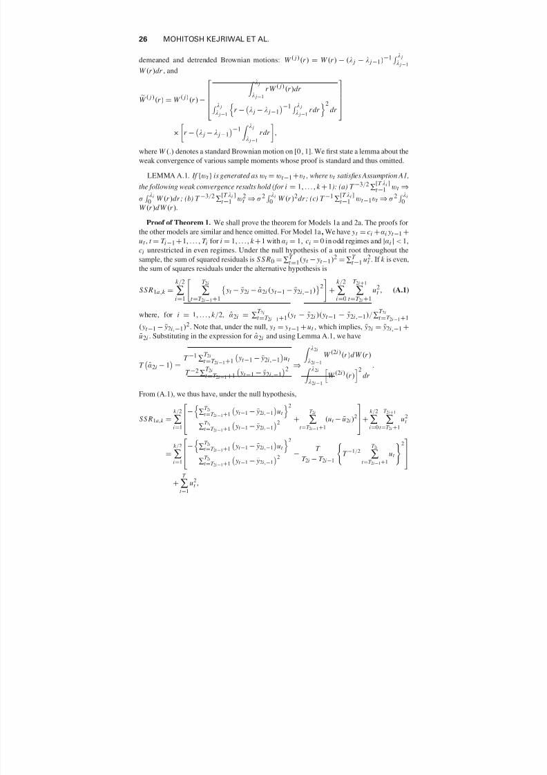
26 MOHITOSH KEJRIWAL ET AL.
demeaned and detrended Brownian motions: W ( j )(r ) = W (r ) − (λ j − λ j −1)−1 λ j
λ j −1
W (r )dr , and
W ( j )(r ) = W ( j )(r ) − λ j
λ j−1r W
( j)
(r )dr λ j
λ j−1
r −
λ j − λ j−1
−1 λ j
λ j−1r dr
2dr
×
r −
λ j − λ j −1
−1 λ j
λ j −1
r dr
,
where W (.) denotes a standard Brownian motion on [0, 1]. We first state a lemma about the
weak convergence of various sample moments whose proof is standard and thus omitted.
LEMMA A.1. If {wt } is generated as wt = wt −1
+v t , where v t satisfies Assumption A1,
the following weak convergence results hold (for i = 1, . . . , k + 1): (a) T −3/2∑
[T λi ]t =1 wt ⇒
σ λi
0 W (r )dr ; (b) T −3/2∑
[T λi ]t =1 w2
t ⇒ σ 2 λi
0 W (r )2dr ; (c) T −1∑
[T λi ]t =1 wt −1v t ⇒ σ 2
λi
0W (r )d W (r ).
Proof of Theorem 1. We shall prove the theorem for Models 1a and 2a. The proofs for
the other models are similar and hence omitted. For Model 1a, We have yt = ci + αi yt −1 +
ut , t = T i −1 + 1, . . . , T i for i = 1, . . . , k + 1 with αi = 1, ci = 0 in odd regimes and |αi | < 1,
ci unrestricted in even regimes. Under the null hypothesis of a unit root throughout the
sample, the sum of squared residuals is S S R0 = ∑T t =1( yt − yt −1)2 = ∑
T t =1 u2
t . If k is even,
the sum of squares residuals under the alternative hypothesis is
S S R1a,k =k /2
∑i =1
T 2i
∑t =T 2i−1+1
yt − ¯ y2i − α2i ( yt −1 − ¯ y2i,−1)
2
+
k /2
∑i=0
T 2i+1
∑t =T 2i +1
u2t , (A.1)
where, for i = 1, . . . , k /2, α2i = ∑T 2it =T 2i −1+1( yt − ¯ y2i )( yt −1 − ¯ y2i,−1)/∑
T 2it =T 2i −1+1
( yt −1 − ¯ y2i,−1)2. Note that, under the null, yt = yt −1 + ut , which implies, ¯ y2i = ¯ y2i,−1 +
u2i . Substituting in the expression for α2i and using Lemma A.1, we have
T α2i − 1= T
−1
∑
T 2i
t =T 2i −1+1 yt −1 − ¯ y2i,−1ut
T −2 ∑T 2i
t =T 2i −1+1
yt −1 − ¯ y2i,−1
2 ⇒
λ2i
λ2i −1
W (2i )(r )d W (r ) λ2i
λ2i−1
W (2i)(r )
2dr
.
From (A.1), we thus have, under the null hypothesis,
SS R1a,k =k /2
∑i=1
−∑
T 2i
t =T 2i −1+1
yt −1 − ¯ y2i,−1
ut
2
∑T 2i
t =T 2i −1+1
yt −1 − ¯ y2i,−1
2 +
T 2i
∑t =T 2i−1+1
(ut − u2i )2
+k /2
∑i=0
T 2i+1
∑t =T 2i +1
u2t
=
k /2
∑i=1
−∑T 2i
t =T 2i −1+1 yt −1 − ¯ y2i,−1ut 2
∑T 2i
t =T 2i −1+1
yt −1 − ¯ y2i,−1
2 − T T 2i − T 2i−1
T −1/2
T 2i
∑t =T 2i −1+1
ut 2+
T
∑t =1
u2t ,
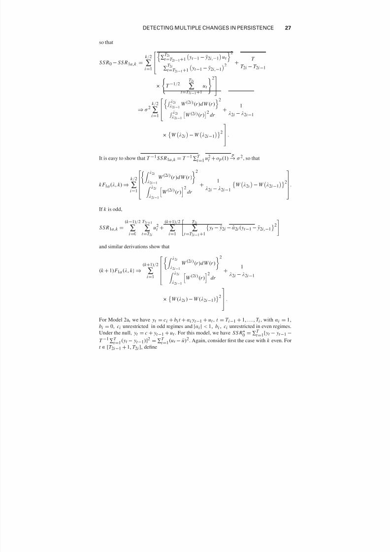
7/25/2019 WALD TESTS FOR DETECTING MULTIPLE STRUCTURAL CHANGES IN PERSISTENCE
http://slidepdf.com/reader/full/wald-tests-for-detecting-multiple-structural-changes-in-persistence 27/35
DETECTING MULTIPLE CHANGES IN PERSISTENCE 27
so that
S S R0 − SS R1a,k =
k /2
∑i =1∑
T 2it =T 2i−1+1 yt −1 − ¯ y2i,−1ut
2
∑T 2it =T 2i−1+1
yt −1 − ¯ y2i,−12 +
T
T 2i − T 2i −1
×
T −1/2
T 2i
∑t =T 2i −1+1
ut
2
⇒ σ 2k /2
∑i=1
λ2i
λ2i−1W (2i)(r )d W (r )
2
λ2iλ2i−1
W (2i )(r )
2dr
+ 1
λ2i − λ2i−1
×
W
λ2i
− W
λ2i −1
2 .
It is easy to show that T −1 SS R1a,k = T −1∑
T t =1 u2
t + o p(1) p→ σ 2, so that
k F 1a (λ, k ) ⇒k /2
∑
i =1
λ2i
λ2i −1
W (2i)(r )d W (r )
2
λ2i
λ2i−1W
(2i )
(r )2
dr
+ 1
λ2i − λ2i −1 W
λ2i
− W
λ2i −1
2
.
If k is odd,
S S R1a,k =(k −1)/2
∑i =0
T 2i+1
∑t =T 2i
u2t +
(k +1)/2
∑i =1
T 2i
∑t =T 2i−1+1
yt − ¯ y2i − α2i ( yt −1 − ¯ y2i,−1
2
and similar derivations show that
(k + 1)F 1a (λ, k ) ⇒(k +1)/2
∑i=1
λ2i
λ2i−1
W (2i)(r )d W (r )2
λ2i
λ2i−1
W (2i)(r )
2dr
+ 1
λ2i − λ2i −1
×
W (λ2i ) − W (λ2i −1)2
.
For Model 2a, we have yt = ci + bi t + αi yt −1 + ut , t = T i −1 + 1, . . . , T i , with αi = 1,bi = 0, ci unrestricted in odd regimes and |αi | < 1, bi , ci unrestricted in even regimes.
Under the null, yt = c + yt −1 + ut . For this model, we have S S R∗0 = ∑
T t =1[ yt − yt −1 −
T −1∑
T t =1( yt − yt −1)]2 = ∑
T t =1(ut − u)2. Again, consider first the case with k even. For
t ∈ [T 2i−1 + 1, T 2i ], define
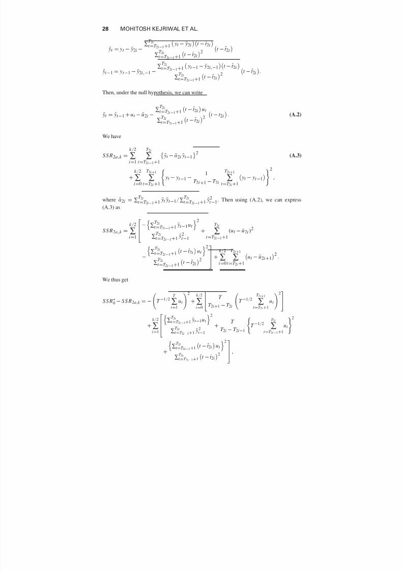
7/25/2019 WALD TESTS FOR DETECTING MULTIPLE STRUCTURAL CHANGES IN PERSISTENCE
http://slidepdf.com/reader/full/wald-tests-for-detecting-multiple-structural-changes-in-persistence 28/35
28 MOHITOSH KEJRIWAL ET AL.
˜ yt = yt − ¯ y2i −∑
T 2it =T 2i −1+1
yt − ¯ y2i
t − t 2i
∑
T 2it =T 2i −1+1
t − t 2i
2
t − t 2i
˜ yt −1 = yt −1 − ¯ y2i,−1 − ∑T 2it =T 2i −1+1 yt −1 − ¯ y2i,−1t − t 2i
∑T 2it =T 2i−1+1
t − t 2i
2
t − t 2i
.
Then, under the null hypothesis, we can write
˜ yt = ˜ yt −1 + ut − u2i −∑
T 2it =T 2i −1+1
t − t 2i
ut
∑T 2i
t =T 2i −1+1
t − t 2i
2
t − t 2i
. (A.2)
We have
S S R2a,k =k /2
∑i =1
T 2i
∑t =T 2i−1+1
˜ yt − α2i ˜ yt −1
2(A.3)
+k /2
∑i =0
T 2i +1
∑t =T 2i +1
yt − yt −1 −
1
T 2i +1 − T 2i
T 2i+1
∑t =T 2i +1
yt − yt −1
2
,
where α2i = ∑T
2it =T 2i −1+1 ˜ yt ˜ yt −1/∑T
2it =T 2i −1+1 ˜ y2t −1. Then using (A.2), we can express(A.3) as
S S R2a,k =k /2
∑i =1
−∑
T 2it =T 2i−1+1 ˜ yt −1ut
2
∑T 2it =T 2i −1+1 ˜ y2
t −1
+T 2i
∑t =T 2i −1+1
(ut − u2i )2
−
∑
T 2it =T 2i−1+1
t − t 2i
ut
2
∑T 2i
t =T 2i−1+1 t − t 2i2
+k /2
∑i =0
T 2i+1
∑t =T
2i+1
ut − u2i +1
2
.
We thus get
S S R∗0 − S S R2a,k = −
T −1/2
T
∑t =1
ut
2
+k /2
∑i=0
T
T 2i +1 − T 2i
T −1/2
T 2i+1
∑t =T 2i +1
ut
2
+k /2
∑i=1
∑
T 2i
t =T 2i−1+1 ˜ yt −1ut
2
∑
T 2i
t =T 2i−1+1 ˜ y2
t −1
+ T
T 2i
− T 2i−1 T −1/2
T 2i
∑t =T 2i −1+1
ut 2
+
∑
T 2i
t =T 2i−1+1
t − t 2i
ut
2
∑T 2i
t =T 2i−1+1
t − t 2i
2
,
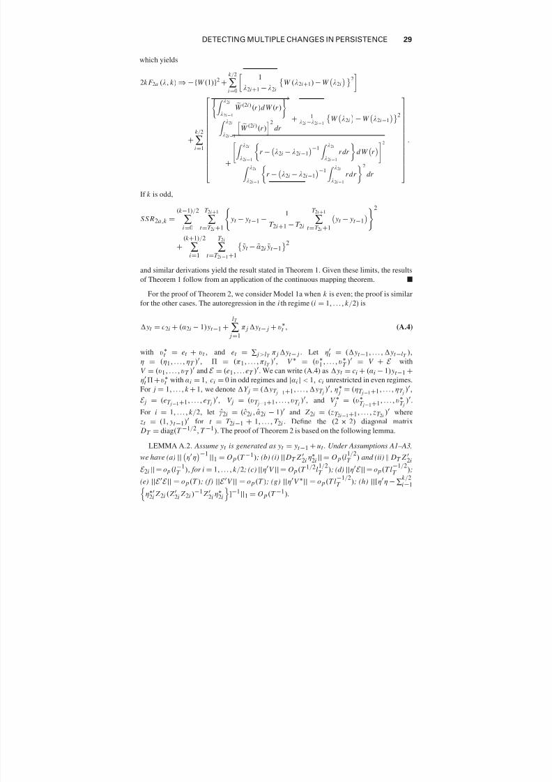
7/25/2019 WALD TESTS FOR DETECTING MULTIPLE STRUCTURAL CHANGES IN PERSISTENCE
http://slidepdf.com/reader/full/wald-tests-for-detecting-multiple-structural-changes-in-persistence 29/35
DETECTING MULTIPLE CHANGES IN PERSISTENCE 29
which yields
2k F 2a (λ, k ) ⇒ − {W (1)}2 +k /2
∑i=0
1
λ2i+1 − λ2i W (λ2i+1) − W λ2i2
+k /2
∑i =1
λ2i
λ2i −1
W (2i)(r )d W (r )
2
λ2i
λ2i−1
W (2i )(r )2
dr
+ 1λ2i −λ2i −1
W
λ2i
− W
λ2i−1
2
+
λ2i
λ2i −1
r −
λ2i − λ2i −1
−1 λ2i
λ2i −1
r dr
d W
r 2
λ2i
λ2i −1r −λ2i − λ2i−1−1
λ2i
λ2i −1
r dr 2
dr
.
If k is odd,
S S R2a,k =(k −1)/2
∑i =0
T 2i+1
∑t =T 2i +1
yt − yt −1 −
1
T 2i+1 − T 2i
T 2i+1
∑t =T 2i +1
yt − yt −1
2
+(k +1)/2
∑i=1
T 2i
∑t =T 2i −1+1
˜ yt − α2i ˜ yt −1
2
and similar derivations yield the result stated in Theorem 1. Given these limits, the resultsof Theorem 1 follow from an application of the continuous mapping theorem.
For the proof of Theorem 2, we consider Model 1a when k is even; the proof is similar
for the other cases. The autoregression in the i th regime (i = 1, . . . , k /2) is
yt = c2i + (α2i − 1) yt −1 +lT
∑ j =1
π j yt − j + v ∗t , (A.4)
with v ∗t = et + v t , and et = ∑ j >lT
π j yt − j . Let ηt = ( yt −1, . . . , yt −lT
),
η = (η1, . . . , ηT )
, = (π1, . . . , πlT )
, V
∗
= (v
∗
1 , . . . , v
∗
T )
= V + E
withV = (v 1, . . . , v T )
and E = (e1, . . . eT ). We can write (A.4) as yt = ci + (αi − 1) yt −1 +
ηt + v ∗
t with αi = 1, ci = 0 in odd regimes and |αi | < 1, ci unrestricted in even regimes.
For j = 1, . . . , k + 1, we denote Y j = ( yT j −1+1, . . . , yT j ), η∗ j = (ηT j−1+1, . . . , ηT j ),
E j = (eT j −1+1, . . . , eT j ), V j = (v T j−1+1, . . . , v T j ), and V ∗ j = (v ∗T j−1+1, . . . , v ∗
T j).
For i = 1, . . . , k /2, let γ2i = (c2i , α2i − 1) and Z 2i = ( zT 2i−1+1, . . . , zT 2i) where
zt = (1, yt −1) for t = T 2i −1 + 1, . . . , T 2i . Define the (2 × 2) diagonal matrix
DT = diag(T −1/2, T −1). The proof of Theorem 2 is based on the following lemma.
LEMMA A.2. Assume yt is generated as yt = yt −1 + ut . Under Assumptions A1–A3,
we have (a) || ηη−1 ||1 = O p(T −1); (b) (i) || DT Z 2i η∗2i || = O p(l1/2T ) and (ii) || DT Z 2i
E 2i || = o p(l−1T ), for i = 1, . . . , k /2; (c) ||ηV || = O p(T 1/2l
1/2T ); (d) ||η
E || = o p(T l−1/2T );
(e) ||E E || = o p(T ); (f) ||E
V || = o p(T ); (g) ||ηV ∗|| = o p(T l−1/2T ); (h) ||[ηη − ∑
k /2i =1
η∗2i Z 2i ( Z 2i Z 2i )−1 Z 2i η∗
2i
]−1||1 = O p(T −1).
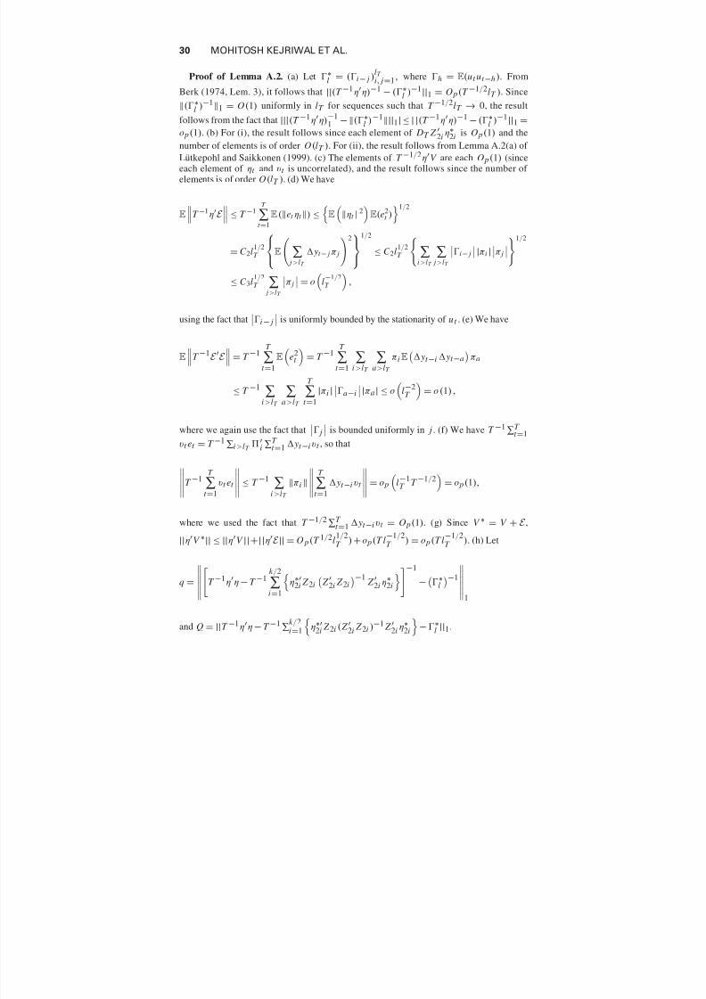
7/25/2019 WALD TESTS FOR DETECTING MULTIPLE STRUCTURAL CHANGES IN PERSISTENCE
http://slidepdf.com/reader/full/wald-tests-for-detecting-multiple-structural-changes-in-persistence 30/35
30 MOHITOSH KEJRIWAL ET AL.
Proof of Lemma A.2. (a) Let ∗l = (i − j )
lT i, j =1, where h = E(ut ut −h ). From
Berk (1974, Lem. 3), it follows that ||(T −1ηη)−1 − (∗l )−1||1 = O p(T −1/2lT ). Since
(∗l )−11 = O(1) uniformly in lT for sequences such that T −1/2lT → 0, the result
follows from the fact that |||(T −1ηη)−11 − (∗
l )−1||1| ≤ | |(T −1ηη)−1 − (∗l )−1||1 =
o p(1). (b) For (i), the result follows since each element of DT Z 2i η∗2i is O p(1) and the
number of elements is of order O(lT ). For (ii), the result follows from Lemma A.2(a) of
Lutkepohl and Saikkonen (1999). (c) The elements of T −1/2ηV are each O p(1) (sinceeach element of ηt and v t is uncorrelated), and the result follows since the number of elements is of order O(lT ). (d) We have
E
T −1η
E
≤ T −1
T
∑t =1
E(et ηt ) ≤
E
ηt
2
E(e2
t )
1/2
= C 2l1/2T
E
∑
j >lT
yt − j π j
21/2
≤ C 2l1/2T
∑
i >lT
∑ j>lT
i − j
|πi |π j
1/2
≤ C 3l1/2T ∑
j>lT
π j
= o
l−1/2T
,
using the fact thati − j
is uniformly bounded by the stationarity of u t . (e) We have
ET −1
E E = T −1 T
∑t =1
Ee2
t = T −1 T
∑t =1
∑i >lT
∑a>lT
πiE yt −i yt −a
πa
≤ T −1∑
i >lT
∑a>lT
T
∑t =1
|πi |a−i
|πa | ≤ o
l−2T
= o (1) ,
where we again use the fact that j
is bounded uniformly in j . (f) We have T −1∑
T t =1
v t et = T −1∑i>lT
i ∑
T t =1 yt −i v t , so that
T −1T
∑t =1
v t et
≤ T −1 ∑i >lT
πi
T
∑t =1
yt −i v t
= o p
l
−1T T −1/2
= o p(1),
where we used the fact that T −1/2 ∑T t =1 yt −i v t = O p(1). (g) Since V ∗ = V + E ,
||ηV ∗|| ≤ ||ηV ||+||ηE || = O p(T 1/2l
1/2T ) + o p(T l
−1/2T ) = o p(T l
−1/2T ). (h) Let
q = T −1ηη − T −1
k /2
∑i=1η∗2i Z 2i Z 2i Z 2i −1
Z 2i η∗2i−1
−∗l −11
and Q = ||T −1ηη − T −1∑
k /2i =1
η∗
2i Z 2i ( Z 2i Z 2i )−1 Z 2i η∗2i
− ∗
l ||1.
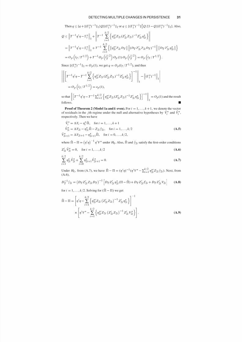
7/25/2019 WALD TESTS FOR DETECTING MULTIPLE STRUCTURAL CHANGES IN PERSISTENCE
http://slidepdf.com/reader/full/wald-tests-for-detecting-multiple-structural-changes-in-persistence 31/35
DETECTING MULTIPLE CHANGES IN PERSISTENCE 31
Then q ≤ {q +(∗l )−11}Q(∗
l )−11 or q ≤ (∗l )−12
1 Q/[1 − Q(∗l )−11]. Also,
Q ≤ T −1ηη − ∗l 1
+T −1k /2
∑i =1η∗
2i Z 2i ( Z 2i Z 2i )−1 Z 2i η∗2i
=T −1ηη − ∗
l
1
+ T −1k /2
∑i =1
η∗2i Z 2i DT
( DT Z 2i Z 2i DT )−1 DT Z 2i η∗
2i
= O p
lT / T 1/2
+ T −1 O p
l
1/2T
O p (1) O p
l
1/2T
= O p
lT /T 1/2
.
Since (∗l )−11 = O p (1), we get q = O p(lT / T 1/2), and thus
T −1ηη − T −1k /2
∑i=1η∗
2i Z 2i ( Z 2i Z 2i )−1 Z 2i η∗2i
−1
1
−(∗l )−11
= O p
lT / T 1/2
= o p(1),
so that
T −1ηη − T −1∑
k /2i =1
η∗
2i Z 2i ( Z 2i Z 2i )−1 Z 2i η∗2i
−1
1
= O p(1) and the result
follows.
Proof of Theorem 2 (Model 1a and k even). For i = 1, . . . , k + 1, we denote the vector
of residuals in the j th regime under the null and alternative hypotheses by V ∗i and V ∗i ,
respectively. Then we have
V ∗i = Y i − η∗i
, for i = 1, . . . , k + 1
V ∗2i = Y 2i − η∗2i
− Z 2i γ2i , for i = 1, . . . , k /2 (A.5)
V ∗2i +1 = Y 2i +1 − η∗2i +1
, for i = 0, . . . , k /2,
where − =
ηη−1
ηV ∗ under H 0. Also, and γ2i satisfy the first-order conditions
Z 2i V ∗2i = 0, for i = 1, . . . , k /2 (A.6)
k /2
∑i=1
η∗2i V ∗2i +
k /2
∑i=0
η∗2i+1 V ∗2i +1 = 0. (A.7)
Under H 0, from (A.7), we have − = (ηη)−1(ηV ∗ −∑k /2i=1 η∗
2i Z 2i γ2i ). Next, from
(A.6),
D−1T γ2i =
DT Z 2i Z 2i DT
−1
DT Z 2i η∗2i ( − ) + DT Z 2i E 2i + DT Z 2i V 2i
(A.8)
for i = 1, . . . , k /2. Solving for ( − ) we get
− = ηη −k /2
∑i =1
η∗2i Z 2i Z 2i Z 2i −1 Z 2i η∗
2i−1
×
η V ∗ −
k /2
∑i =1
η∗
2i Z 2i
Z 2i Z 2i
−1 Z 2i V ∗2i
. (A.9)
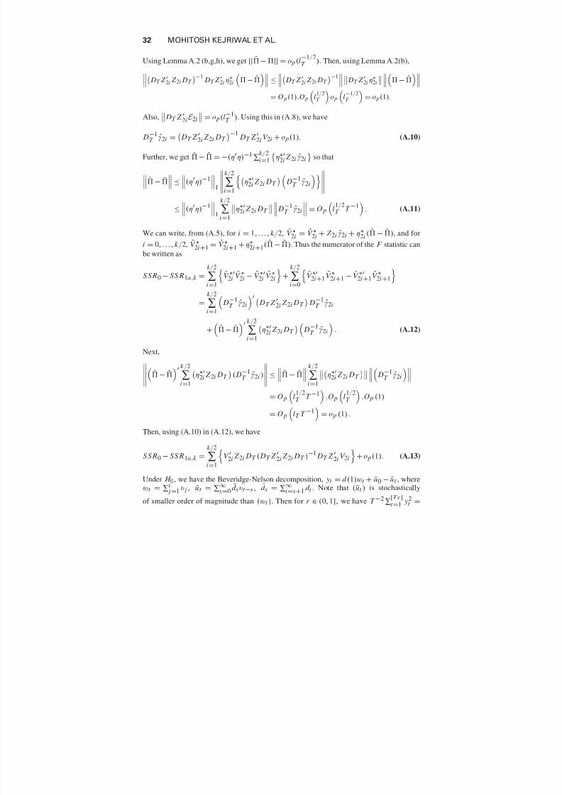
7/25/2019 WALD TESTS FOR DETECTING MULTIPLE STRUCTURAL CHANGES IN PERSISTENCE
http://slidepdf.com/reader/full/wald-tests-for-detecting-multiple-structural-changes-in-persistence 32/35
32 MOHITOSH KEJRIWAL ET AL.
Using Lemma A.2 (b,g,h), we get || − || = o p (l−1/2T ). Then, using Lemma A.2(b),
DT Z 2i Z 2i DT
−1
DT Z 2i η∗2i
−
≤
DT Z 2i Z 2i DT
−1
DT Z 2i η∗
2i −
= O p(1).O p l1/2T o p l−1/2
T = o p(1).
Also, DT Z 2i E 2i
= o p(l−1T ). Using this in (A.8), we have
D−1T γ2i =
DT Z 2i Z 2i DT
−1 DT Z 2i V 2i + o p (1). (A.10)
Further, we get − = −(ηη)−1∑
k /2i =1
η∗
2i Z 2i γ2i
so that
ˆ −
˜≤ (η
η)
−11k /2
∑i =1η
∗
2i Z 2i DT D
−1
T γ2i≤(ηη)−1
1
k /2
∑i =1
η∗2i Z 2i DT
D−1T γ2i
= O p
l
1/2T T −1
. (A.11)
We can write, from (A.5), for i = 1, . . . , k /2, V ∗2i = V ∗2i + Z 2i γ2i + η∗2i ( − ), and for
i = 0, . . . , k /2, V ∗2i +1 = V ∗2i +1 + η∗2i +1( − ). Thus the numerator of the F statistic can
be written as
S S R0 − SS R1a,k =
k /2
∑i=1 V
∗2i V
∗2i − V
∗2i V
∗2i+
k /2
∑i=0 V
∗2i +1 V
∗2i+1 − V
∗2i+1 V
∗2i +1
=k /2
∑i=1
D−1
T γ2i
DT Z 2i Z 2i DT
D−1
T γ2i
+
− k /2
∑i=1
η∗
2i Z 2i DT
D−1
T γ2i
. (A.12)
Next,
− k /2
∑i =1
η∗2i Z 2i DT ( D−1
T γ2i ) ≤ − k /2
∑i =1
η∗2i Z 2i DT D−1
T γ2i= O p
l
1/2T T −1
.O p
l
1/2T
.O p (1)
= O p
lT T −1
= o p (1) .
Then, using (A.10) in (A.12), we have
S S R0 − SS R1a,k =k /2
∑i=1V 2i Z 2i DT ( DT Z 2i Z 2i DT )
−1 DT Z 2i V 2i+ o p(1). (A.13)
Under H 0, we have the Beveridge-Nelson decomposition, yt = d (1)wt + u0 − ut , wherewt = ∑
t j =1 v j , ut = ∑
∞s=0
d s v t −s , d s = ∑∞i =s+1 d i . Note that (ut ) is stochastically
of smaller order of magnitude than (wt ). Then for r ∈ (0, 1], we have T −2∑
[T r ]t =1 y2
t =
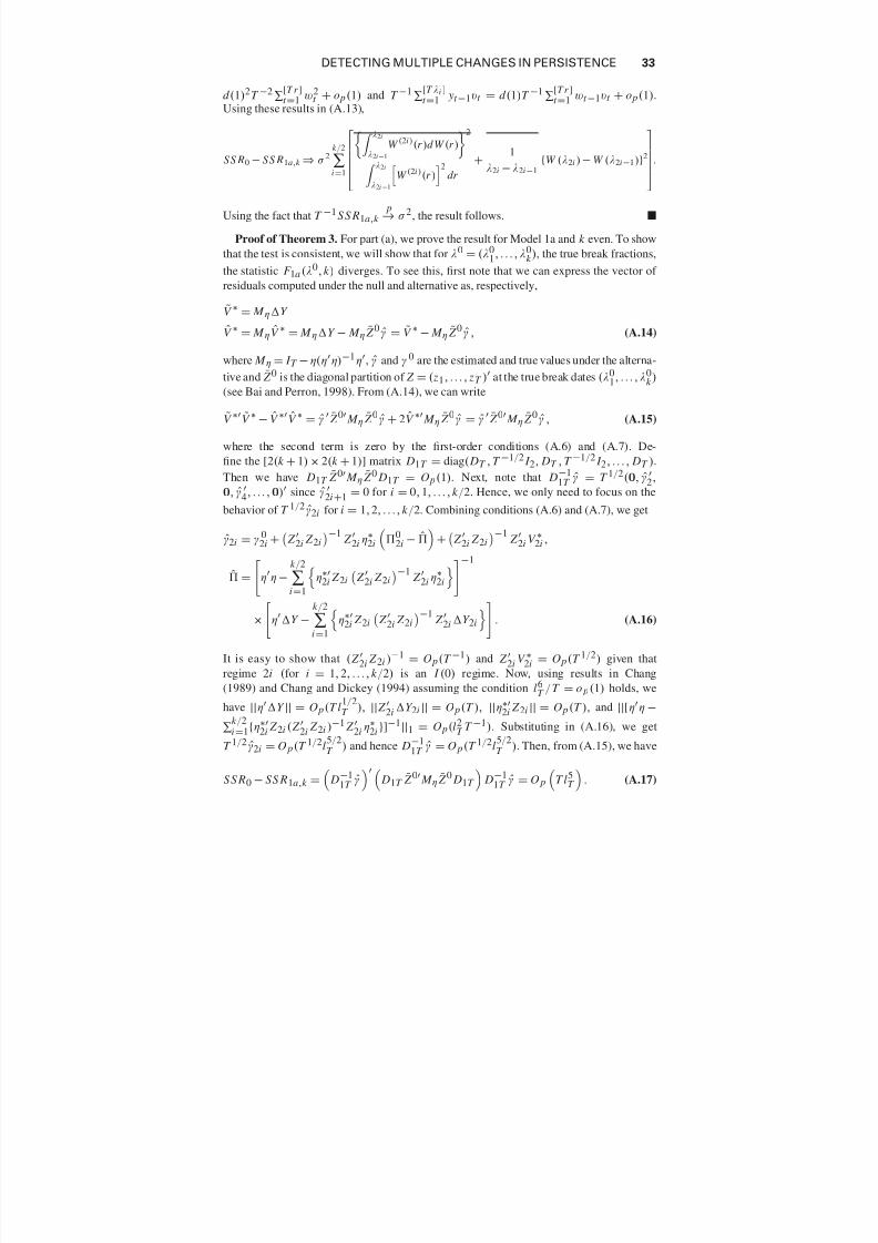
7/25/2019 WALD TESTS FOR DETECTING MULTIPLE STRUCTURAL CHANGES IN PERSISTENCE
http://slidepdf.com/reader/full/wald-tests-for-detecting-multiple-structural-changes-in-persistence 33/35
DETECTING MULTIPLE CHANGES IN PERSISTENCE 33
d (1)2T −2∑
[T r ]t =1 w2
t + o p(1) and T −1∑
[T λi ]t =1 yt −1v t = d (1)T −1
∑[T r ]t =1 wt −1v t + o p(1).
Using these results in (A.13),
SS R0 − SS R1a,k ⇒ σ 2k /2
∑i =1
λ2i
λ2i −1W (2i )(r )d W (r )2
λ2i
λ2i −1
W (2i )(r )
2dr
+ 1
λ2i − λ2i −1
{W (λ2i ) − W (λ2i −1)}2.
Using the fact that T −1 S S R1a,k p
→ σ 2, the result follows.
Proof of Theorem 3. For part (a), we prove the result for Model 1a and k even. To show
that the test is consistent, we will show that for λ0 = (λ01, . . . , λ0
k ), the true break fractions,
the statistic F 1a (λ0, k ) diverges. To see this, first note that we can express the vector of
residuals computed under the null and alternative as, respectively,
V ∗ = M ηY
V ∗ = M η V ∗ = M ηY − M η ¯ Z 0γ = V ∗ − M η ¯ Z 0γ , (A.14)
where M η = I T − η(ηη)−1η, γ and γ 0 are the estimated and true values under the alterna-
tive and ¯ Z 0 is the diagonal partition of Z = ( z1, . . . , zT ) at the true break dates (λ0
1, . . . , λ0k )
(see Bai and Perron, 1998). From (A.14), we can write
V ∗ V ∗ − V ∗ V ∗ = γ ¯ Z 0 M η ¯ Z 0γ + 2 V ∗ M η ¯ Z 0γ = γ ¯ Z 0 M η ¯ Z 0γ , (A.15)
where the second term is zero by the first-order conditions (A.6) and (A.7). De-
fine the [2(k + 1) × 2(k + 1)] matrix D1T = diag( DT , T −1/2 I 2, DT , T −1/2 I 2, . . . , DT ).
Then we have D1T ¯ Z 0 M η ¯ Z 0 D1T = O p(1). Next, note that D
−11T γ = T 1/2(0, γ
2,
0, γ 4, . . . ,0) since γ
2i +1 = 0 for i = 0, 1, . . . , k /2. Hence, we only need to focus on the
behavior of T 1/2γ2i for i = 1, 2, . . . , k /2. Combining conditions (A.6) and (A.7), we get
γ2i = γ 02i +
Z 2i Z 2i
−1 Z 2i η∗
2i
0
2i −
+ Z 2i Z 2i
−1 Z 2i V ∗2i ,
= η
η −
k /2
∑i =1η
∗2i Z 2i Z
2i Z 2i −1
Z 2i η
∗2i
−1
×
ηY −
k /2
∑i =1
η∗
2i Z 2i
Z 2i Z 2i
−1 Z 2i Y 2i
. (A.16)
It is easy to show that ( Z 2i Z 2i )−1 = O p(T −1) and Z 2i V ∗2i = O p(T 1/2) given that
regime 2i (for i = 1, 2, . . . , k /2) is an I (0) regime. Now, using results in Chang
(1989) and Chang and Dickey (1994) assuming the condition l6T / T = o p(1) holds, we
have ||ηY || = O p(T l1/2T ), || Z 2i Y 2i || = O p(T ), ||η∗
2i Z 2i || = O p (T ), and ||[ηη −
∑k /2i =1{η∗2i Z 2i ( Z 2i Z 2i )−1 Z 2i η∗2i }]−1||1 = O p(l2T T −1). Substituting in (A.16), we get
T 1/2γ2i = O p(T 1/2l5/2T ) and hence D
−11T γ = O p(T 1/2l
5/2T ). Then, from (A.15), we have
S S R0 − SS R1a,k =
D−11T γ
D1T
¯ Z 0 M η ¯ Z 0 D1T
D−1
1T γ = O p
T l5
T
. (A.17)
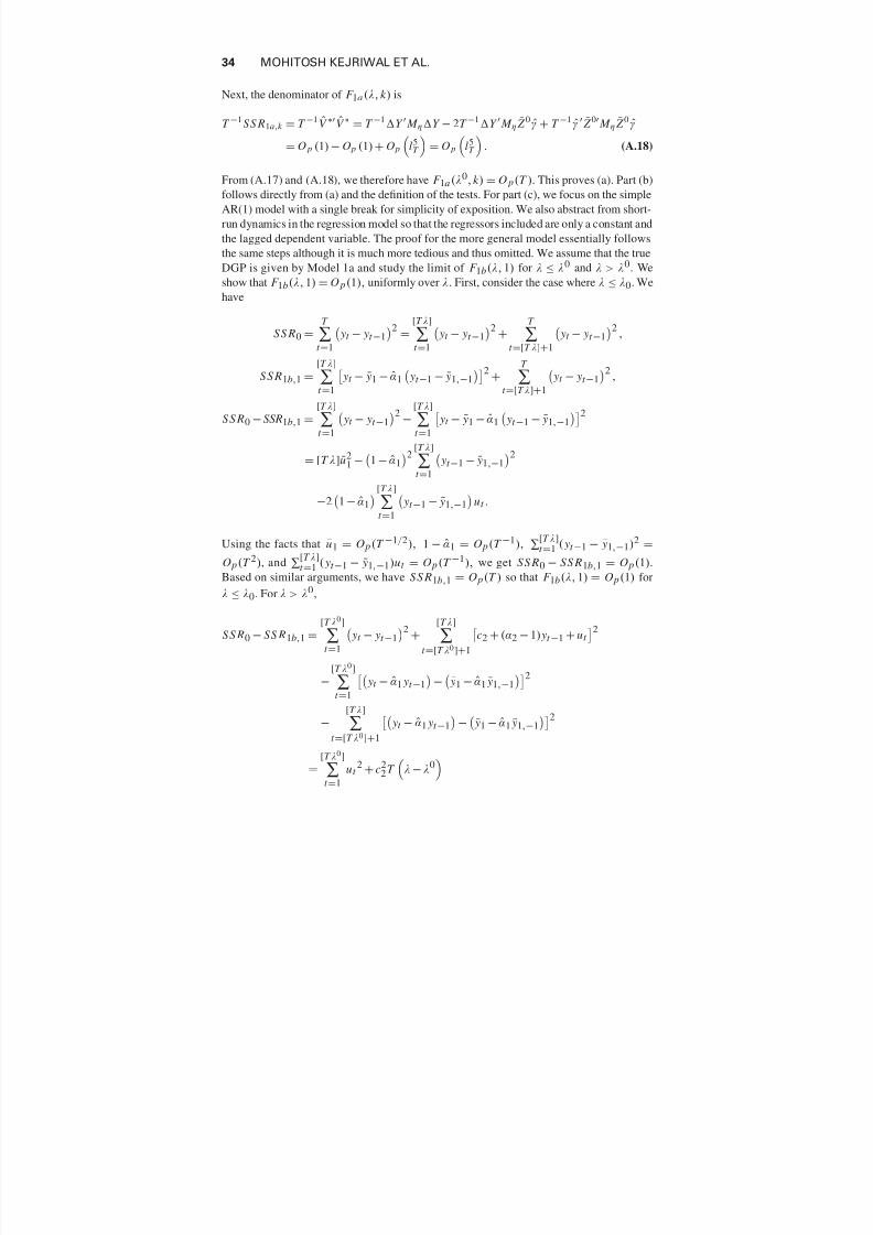
7/25/2019 WALD TESTS FOR DETECTING MULTIPLE STRUCTURAL CHANGES IN PERSISTENCE
http://slidepdf.com/reader/full/wald-tests-for-detecting-multiple-structural-changes-in-persistence 34/35
34 MOHITOSH KEJRIWAL ET AL.
Next, the denominator of F 1a (λ, k ) is
T −1 S S R1a,k = T −1 V ∗ V ∗ = T −1Y M ηY − 2T −1Y M η ¯ Z 0γ + T −1γ ¯ Z 0 M η ¯ Z 0γ
= O p (1) − O p (1) + O p l5T = O p l5T . (A.18)
From (A.17) and (A.18), we therefore have F 1a (λ0, k ) = O p(T ). This proves (a). Part (b)
follows directly from (a) and the definition of the tests. For part (c), we focus on the simple
AR(1) model with a single break for simplicity of exposition. We also abstract from short-
run dynamics in the regression model so that the regressors included are only a constant and
the lagged dependent variable. The proof for the more general model essentially follows
the same steps although it is much more tedious and thus omitted. We assume that the true
DGP is given by Model 1a and study the limit of F 1b(λ, 1) for λ ≤ λ0 and λ > λ0. We
show that F 1b(λ, 1) = O p(1), uniformly over λ. First, consider the case where λ ≤ λ0. Wehave
S S R0 =T
∑t =1
yt − yt −1
2=
[T λ]
∑t =1
yt − yt −1
2+
T
∑t =[T λ]+1
yt − yt −1
2,
S S R1b,1 =[T λ]
∑t =1
yt − ¯ y1 − α1
yt −1 − ¯ y1,−1
2+
T
∑t =[T λ]+1
yt − yt −1
2,
S S R0 − SSR1b,1 =[T λ]
∑t =1 yt − yt −1
2−
[T λ]
∑t =1 yt − ¯ y1 − α1 yt −1 − ¯ y1,−1
2
= [T λ]u21 −
1 − α1
2[T λ]
∑t =1
yt −1 − ¯ y1,−1
2
−2
1 − α1
[T λ]
∑t =1
yt −1 − ¯ y1,−1
ut .
Using the facts that u1 = O p(T −1/2), 1 − α1 = O p(T −1), ∑[T λ]t =1 ( yt −1 − ¯ y1,−1)2 =
O p(T 2), and ∑[T λ]t =1 ( yt −1 − ¯ y1,−1)ut = O p (T −1), we get S S R0 − SS R1b,1 = O p(1).
Based on similar arguments, we have S S R1b,1 = O p(T ) so that F 1b(λ, 1) = O p(1) forλ ≤ λ0. For λ > λ0,
S S R0 − SS R1b,1 =[T λ0]
∑t =1
yt − yt −1
2+
[T λ]
∑t =[T λ0]+1
c2 + (α2 − 1) yt −1 + ut
2
−[T λ0]
∑t =1
yt − α1 yt −1
−
¯ y1 − α1 ¯ y1,−1
2−
[T λ]
∑t =[T λ0]+1
yt − α1 yt −1− ¯ y1 − α1 ¯ y1,−12
=[T λ0]
∑t =1
ut 2 + c2
2 T
λ − λ0

7/25/2019 WALD TESTS FOR DETECTING MULTIPLE STRUCTURAL CHANGES IN PERSISTENCE
http://slidepdf.com/reader/full/wald-tests-for-detecting-multiple-structural-changes-in-persistence 35/35
DETECTING MULTIPLE CHANGES IN PERSISTENCE 35
+ (α2 − 1)2[T λ]
∑t =[T λ0]+1
y2t −1 +
[T λ]
∑t =[T λ0]+1
u2t + 2c2(α2 − 1)
[T λ]
∑t =[T λ0]+1
yt −1
+ 2c2
[T λ]
∑t =[T λ0]+1
ut + 2(α2 − 1)
[T λ]
∑t =[T λ0]+1
yt −1ut
−[T λ0]
∑t =1
1 − α1
yt −1 + ut −
¯ y1 − α1 ¯ y1,−1
2
−[T λ]
∑t =[T λ0]+1
c2 +
α2 − α1
yt −1 + ut −
¯ y1 − α1 ¯ y1,−1
2
= (α2 − 1)2[T λ]
∑t =[T λ0]+1
y2
t −1
−α2 − α12
×[T λ]
∑t =[T λ0]+1
y2t −1 + 2c2
α1 − 1
[T λ]
∑t =[T λ0]+1
yt −1
+ 2(α1 − 1)[T λ]
∑t =[T λ0]+1
yt −1ut + 2
¯ y1 − α1 ¯ y1,−1
×
[T λ0]
∑t =1
ut +[T λ]
∑t =[T λ
0]+1
ut
−
1 − α1
2[T λ0]
∑t =1
y2t −1
− 2
1 − α1
[T λ0]
∑t =1
yt −1ut + 2
1 − α1
¯ y1 − α1 ¯ y1,−1
×
[T λ0]
∑t =1
yt −1 − [T λ]
¯ y1 − α1 ¯ y1,−1
2
+2
¯ y1 − α1 ¯ y1,−1
T
λ − λ0
α2 − α1
− c2
α1 − α2
−1
+
T
λ − λ0−1 [T λ]
∑t =[T λ0]+1
yt −1
. (A.19)
Now we have ∑[T λ0]t =1 y2
t −1 = O p(T 2), α1 = 1 + O p(T −1), ¯ y1 − α1 ¯ y1,−1 = (1 − α1)
¯ y1,−1 + O p(T −1) = O p(T −1/2), ∑[T λ]
t =[T λ0]+1 y2
t −1 = [T (λ − λ0)]O p(1), ∑[T λ]
t =[T λ0]+1
yt −1ut = [T (λ − λ0)]1/2 O p (1), ∑[T λ]
t =[T λ0]+1ut = [T (λ − λ0)]1/2 O p(1). Note that the
last term in brackets can be expressed as 2( ¯ y1 − α1 ¯ y1,−1)(α2 − α1)∑[T λ]
t =[T λ0]+1( yt −1 −
c2/(α1 − α2)) = O p (T −1/2)O p(1)O p(T 1/2) = O p(1). Substituting these orders in
(A.19), each of the terms in brackets is O p(1). Again, similar arguments can be used to
show that S S R1b,1 = O p(T ) and thus F 1b(λ, 1) = O p(1).