walpole 8 probabilidad y estadística para ciencias e ingenierias parte2
DESCRIPTION
ÂTRANSCRIPT

11.12 Correlation 433
0.6
0.3
-0.3
-0.6
•
•
«
•
•
* •
•
•• •
• • •
•
• •
•
•
• • •
•
*
•
•
•
10 15 Density
20 25
0.6
0.3
-0.3
-0.6
- 2 - 1 0 1 Standard Normal Quantile
Figure 11.26: Residual plot using the log transfer- Figure 11.27: Normal probability plot of residuals mation for the wood density data. using the log transformation for the wood density
data.
In theory it is often assumed that the conditional distribution f(y\x) of Y, for fixed values of X, is normal with mean p.y\x = a + 0x and variance Oy<x = a2 and
that X is likewise normally distributed with mean p, and variance a2. The joint density of X and Y is then
f(x, y) = n(y\x; a + 0x, a)n(x; px, ax)
(y — a — 0x\ ( x 1 2itaxa exp
Px o~x
for —oo < x < oo and —oc < y < ex. Let us write the random variable Y in the form
Y = a + BX + e,
where X is now a random variable independent of the random error e. Since the mean of the random error e is zero, it follows that
py = a + 0px and ay = a2 + 02a\.
Substituting for a and a2 into the preceding expression for fix,y), we obtain the bivariate normal distribution
fix,y) = 1
27TCT,Yay y/\ — O2
x exp f l \(x-px\2 _ 2 fx-px\ (y-PY\ (V-PYV] 1 \ 2(l-(fi)[\ ax J P \ crx J\ ay J + { ay )\f>

434 Chapter 11 Simple Linear Regression and Correlation
for —oo < x < oo and —oo < y < oc, where
p2 = ! _ £_ = , 2fi ^ Oy Oy'
The constant /? (rho) is called the population correlation coefficient and plays a major role in many bivariate data analysis problems. It is important for the reader to understand the physical interpretation of this correlation coefficient and the distinction between correlation and regression. The term regression still has meaning here. In fact, the straight line given by py\x = a + 0x is still called the regression line as before, and the estimates of a and ,3 are identical to those given in Section 11.3. The value of p is 0 when 0 = 0, which results when there essentially is no linear regression; that is, the regression line is horizontal and any knowledge of X is useless in predicting Y. Since aY > a2, we must have p2 < 1 and hence -1 < p < 1. Values of p — ±1 only occur when er2 = 0, in which case we have a perfect linear relationship between the two variables. Thus a value of p equal to +1 implies a perfect linear relationship with a positive slope, while a value of p equal to —1 results from a perfect linear relationship with a negative slope. It might be said, then, that sample estimates of p close to unity in magnitude imply good correlation or linear association between X and Y, whereas values near zero indicate little or no correlation.
To obtain a sample estimate of p, recall from Section 11.4 that the error sum of squares is
o*jii = *-*yy boXy-
Dividing both sides of this equation by Syy and replacing Sxy by bSxx, we obtain the relation
,2 Jxx . SoE -q — I o • °yy Jyy
The value of b2Sxx/Syy is zero when 6 = 0, which will occur when the sample points show no linear relationship. Since Syy > SSE, we conclude that b2Sxx/Sxy
must be between 0 and 1. Consequently, by/Sxx/Syy must range from -1 to +1 , negative values corresponding to lines with negative slopes and positive values to lines with positive slopes. A value of -1 or +1 will occur when SSE = 0, but this is the case where all sample points lie in a straight line. Hence a perfect linear relationship appears in the sample data when by/Sxx/Syy = ±1 . Clearly, the quantity by/Sxx/Syy, which we shall henceforth designate as r, can be used as an estimate of the population correlation coefficient, p. It is customary to refer to the estimate r as the Pearson product-moment correlation coefficient or simply the sample correlation coefficient.
Correlation The measure p of linear association between two variables X and Y is estimated Coefficient by the sample correlation coefficient r, where
r - t V ~ " " ' - ^ ^ / O ^ x O ] yy
For values of r between —1 and +1 we must be careful in our interpretation. For example, values of r equal to 0,3 and 0.6 only mean that we have two positive

11.12 Correlation 435
correlations, one somewhat stronger than the other. It is wrong to conclude that r = 0.6 indicates a linear relationship twice as good as that indicated by the value r = 0.3. On the other hand, if we write
c2 ?.2 _ °xy SSR
-~>XX'~'yy
then r2, which is usually referred to as the sample coefficient of determination, represents the proportion of the variation of Syy explained by the regression of V on x, namely, SSR. That is. r2 expresses the proportion of the total variation in the values of the variable Y that can be accounted for or explained by a linear relationship with the values of the random variable X. Thus a correlation of 0.6 means that 0.36, or 36%, of the total variation of the values of Kin our sample is accounted for by a linear relationship with values of X
Example 11.10:1 It is important that scientific researchers in the area of forest products be able to study correlation among the anatomy and mechanical properties of trees. According to the study Quantitative Anatomical Characteristics of Plantation Grown Loblolly Pine (Pinus Taeda L.) and Cottonwood (Populus deltoides Bart. Ex Marsh.) and Their Relationships to Mechanical Properties conducted by the Department of Forestry and Forest Products at the Virginia Polytechnic Institute and State University, an experiment in which 29 loblolly pines were randomly selected for investigation yielded the data of Table 11.9 on the specific gravity in grams/cm3
and the modulus of rupture in kilopascals (kPa). Compute and interpret the sample correlation coefficient.
Specific Gravity, x (g /cm 3 )
0.414 0.383 0.399 0.402 0.442 0.422 0.466 0.500 0.514 0.530 0.569 0.558 0.577 0.572 0.548
Table 11.9: Data of 29 Loblolly Pines for Example
Modulus of Rupture, y (kPa) 29,186 29,266 26,215 30,162 38,867 37,831 44,576 46,097 59,098 67,705 66,088 78,486 89,869 77,369 67,095
Specific Gravity, x (g /cm 3 )
0.581 0.557 0.550 0.531 0.550 0.556 0.523 0.602 0.569 0.544 0.557 0.530 0.547 0.585
11.10
Modulus of Rupture, V (kPa)
85,156 69,571 84,160 73,466 78,610 67,657 74,017 87,291 86,836 82,540 81,699 82,096 75,657 80,490
Solution: From the data we find that
Sxx = 0.11273, Syy = 11,807,324,805, Sxy = 34,422.27572.

436 Chapter 11 Simple Linear Regression and Correlation
Therefore,
r= , 3 4 > 4 2 2 ' 2 7 5 7 2 = Q.9435.
v/(0.11273)(ll,807,3241805)
A correlation coefficient of 0.9435 indicates a good linear relationship between X and Y. Since r2 = 0.8902, we can say that approximately 89% of the variation in
the values of Y is accounted for by a linear relationship with X. J A test of the special hypothesis p = 0 versus an appropriate alternative is
equivalent to testing ,3 = 0 for the simple linear regression model and therefore the procedures of Section 11.8 using either the ^-distribution with n — 2 degrees of freedom or the F-distribution with 1 and n — 2 degrees of freedom are applicable. However, if one wishes to avoid the analysis-of-variance procedure and compute only the sample correlation coefficient, it can be verified (see Exercise 11.51 on page 438) that the i-value
t =
can also be written as
ry/n — 2
y/T^r2
which, as before, is a value of the statistic T having a ^-distribution with n — 2 degrees of freedom.
Example 11.11:1 For the data of Example 11.10, test the hypothesis that there is no linear association among the variables.
Solution: 1. HQ: p = 0.
2. Hx: p/^0. 3. a = 0.05. 4. Critical region: /; < -2.052 or t > 2.052.
5 . Computations: t = j ^ " ^ = 14.79, P < 0.0001.
6. Decision: Reject the hypothesis of no linear association. J A test of the more general hypothesis p = po against a suitable alternative is
easily conducted from the sample information. If X and Y follow the bivariate normal distribution, the quantity
H&) is a value of a random variable that follows approximately the normal distribution with mean ^ In j ^ and variance l / (n — 3). Thus the test procedure is to compute
yfn z = — ^ l n ( i ± i V h / 1 + ^ V ^ 3 i n (l + r)(l-po)
l-rj \l-po)\ 2 l(l-r)(l + p0)
and compare it with the critical points of the standard normal distribution.
Example 11.12:1 For the data of Example 11.10, test the null hypothesis that p = 0.9 against the alternative that p > 0.9. Use a 0.05 level of significance.

11.12 Correlation 437
• •
{a) No Association (b) Causal Relationship
Figure 11.28: Scatter diagram showing zero correlation.
Solution: 1. HQ: p = 0.9.
2. Hx: p > 0.9.
3. a = 0.05.
4. Critical region: z > 1.645.
5. Computations:
z = V^6
In (1 + 0.9435)(0.1) (1-0.9435)(1.9)
= 1.51. F = 0.0655.
6. Decision: There is certainly some evidence that the correlation coefficient does not exceed 0.9. J
It should be pointed out that in correlation studies, as in linear regression problems, the results obtained are only as good as the model that is assumed. In the correlation techniques studied here, a bivariate normal density is assumed for the variables X and Y, with the mean value of Y at each z-value being linearly related to x. To observe the suitability of the linearity assumption, a preliminary plotting of the experimental data is often helpful. A value of the sample correlation coefficient close to zero will result from data that display a strictly random effect as in Figure 11.28(a), thus implying little or no causal relationship. It is important to remember that the correlation coefficient between two variables is a measure of their linear relationship and that a value of r = 0 implies a lack of linearity and not a lack of association. Hence, if a strong quadratic relationship exists between X and F, as indicated in Figure 11.28(b), we can still obtain a zero correlation indicating a nonlinear relationship.

438
Exercises
Chapter 11 Simple Linear Regression and Correlation
11.49 Compute and interpret the correlation coefficient for the following grades of 6 students selected at random:
Mathematics grade English grade
70 92 80 74 65 83
74 84 63 87 78 90
11.50 Test the hypothesis that p = 0 in Exercise 11.49 against the alternative that p ^ 0. Use a 0.05 level of significance.
11.51 Show the necessary steps in converting the
equation r = s/ssr; to the equivalent form / _ .-yAT^S
11.52 The following data were obtained in a study of the relationship between the weight and chest size of infants at birth:
Weight (kg) Ches t Size (cm) 27T5 29J> 2.15 26.3 4.41 32.2 5.52 36.5 3.21 27.2 4.32 27.7 2.31 28.3 4.30 30.3 3.71 28.7
(a) Calculate r.
(b) Test the null hypothesis that p = 0 against the alternative that p > 0 at the 0.0i level of significance.
(c) What percentage of the variation in the infant chest sizes is explained by difference in weight?
11.53 With reference to Exercise 11.1 on page 397, assume that x and y are random variables with a bi-variate normal distribution: (a) Calculate r.
(b) Test the hypothesis that p = 0 against the alternative that p 7 0 at the 0.05 level of significance.
11.54 With reference to Exercise 11.9 on page 399, assume a bivariate normal distribution for x and y.
(a) Calculate r. (b) Test the null hypothesis that p = —0.5 against the
alternative that p < —0.5 at the 0.025 level of significance.
(c) Determine the percentage of the variation in the amount of particulate removed that is due to changes in the daily amount of rainfall.
Review Exercises
11.55 With reference to Exercise 11.6 on page 398, conclusions, construct (a) a 95% confidence interval for the average course
grade of students who make a 35 on the placement test;
(b) a 95% prediction interval for the course grade of a student who made a 35 on the placement test.
11.56 The Statistics Consulting Center at Virginia Polytechnic Institute and State University analyzed data on normal woodchucks for the Department of Veterinary Medicine. The variables of interest were body-weight in grams and heart weight in grams. It was also of interest to develop a linear regression equation in order to determine if there is a significant linear relationship between heart weight and total body weight. Use heart weight as the independent variable and body weight as the dependent variable and fit a simple linear regression using the following data. In addition, test the hypothesis HQ: 3 = 0 versus Hi: 0 •£ 0. Draw
Body Weight grains) 4050 2465 3120 5700 2595 3640 2050 4235 2935 4975 3690 2800 2775 2170 2370 2055 2025 2645 2675
Heart Weight (grams) 11.2 12.4 10.5 13.2 9.8 11.0 10.8 10.4 12.2 11.2 10.8 14.2 12.2 10.0 12.3 12.5 11.8 16.0 13.8

Review Exercises 439
11.57 The amounts of solids removed from a particular material when exposed to drying periods of different lengths are as shown.
x (hours) y (grams) 4.4 4.5 4.8 5.5 5.7 5.9 6.3 6.9 7.5 7.8
13.1 9.0
10.4 13.8 12.7 9.9
13.8 16.4 17.6 18.3
14.2 11.5 11.5 14.8 15.1 12.7 16.5 15.7 16.9 17.2
(a) Estimate the linear regression line.
(b) Test at the 0.05 level of significance whether the linear model is adequate.
11.58 With reference to Exercise 11.7 on page 399, construct
(a) a 95% confidence interval for the average weekly-sales when $45 is spent on advertising;
(b) a 95% prediction interval for the weekly sales when 845 is spent on advertising.
11.59 An experiment was designed for the Department of Materials Engineering at Virginia Polytechnic Institute and State University to study hydrogen ein-brittlement properties based on electrolytic hydrogen pressure measurements. The solution used was 0.1 N NaOH, the material being a certain type of stainless steel. The cathodic charging current density was controlled and varied at four levels. The effective hydrogen pressure was observed as the response. The data follow.
Run 1 2 3 4 5 6 7 8 9
10 11 12 13 14 L5
Charging Current Density, x ( m A / c m 2 )
0.5 0.5 0.5 0.5 1.5 1.5 1.5 2.5 2.5 2.5 2.5 3.5 3.5 3.5 3.5
Effective Hydrogen
Pressure, y (atm) 86.1 92.1 64.7 74.7
223.6 202.1 132.9 413.5 231.5 466.7 365.3 493.7 382.3 447.2 563.8
(b) Compute the pure error sum of squares and make a test for lack of fit.
(c) Does the information in part (b) indicate a need for a model in x beyond a first-order regression? Explain.
11.60 The following data represent the chemistry grades for a random sample of 12 freshmen at a certain college along with their scores on an intelligence test administered while they were still seniors in high school:
Student 1 2 3 4 5 6 7 8 9
10 11 12
Test Score, x
65 50 55 65 55 70 65 70 55 70 50 55
Chemistry Grade, y
85 74 76 90 85 87 94 98 81 91 76 74
(a) Run a simple linear regression of y against x.
(a) Compute and interpret the sample correlation coefficient.
(b) State necessary assumptions on random variables.
(c) Test the hypothesis that p = 0.5 against the alternative that p > 0.5. Use a P-value in the conclusion.
11.61 For the simple linear regression model, prove that E(s2) = a'1.
11.62 The business section of the Washington Times in March of 1997 listed 21 different used computers and printers and their sale prices. Also listed was the average hover bid. Partial results from the regression analysis using SAS software are shown in Figure 11.29 on page 440.
(a) Explain the difference between the confidence interval on the mean and the prediction interval.
(b) Explain why the standard errors of prediction vary from observation to observation.
(c) Which observation has the lowest standard error of prediction? Why?
11.63 Consider the vehicle data in Figure 11.30 from Consumer Reports. Weight is in tons, mileage in miles per gallon, and drive ratio is also indicated. A regression model was fitted relating weight x to mileage y. A partial SAS printout in Figure 11.30 on page 441 shows some of the results of that regression analysis and Fig-

440 Chapter 11 Simple Linear Regression and Correlation
ure 11.31 on page 442 gives plot of the residuals and (b) Fit the model by replacing weight with log weight. weight for each vehicle. (a) From the analysis and the residual plot, does it ap
pear that an improved model might be found by using a transformation? Explain.
Comment on the results, (c) Fit a model by replacing mpg with gallons per 100
miles traveled, as mileage is often reported in other countries. Which of the three models is preferable? Explain.
R-Square Coeff Vax 0.967472 7.923338
Parameter Estimate In te rcep t 59.93749137 Buyer 1.04731316
Root MSE Pr ice Mean 70.83841
Standard Error
38.34195754
product Buyer IBM PS/1 486/66 420MB IBM ThinkPad 500 IBM Think-Dad 755CX AST Pentium 90 540MB Dell Pentium 75 1GB Gateway 486/75 320MB Clone 586/133 1GB Compaq Contura 4/25 120MB Compaq Deskpro P90 1.2GB Micron P75 810MB Micron P100 1.2GB Mac Quadra 840AV 500MB Mac Performer 6116 700MB PouerBook 540c 320MB PowerBook 5300 500MB Power Mac 7500/100 1GB NEC Versa 486 340MB Toshiba 1960CS 320MB Toshiba 4800VCT 500MB HP Laser j e t I I I Apple Laser Writer Pro 63
325 450
1700 800 650 700 500 450 BOO 800 900 450 700
1400 1350 1150 800 700
1000 350 750
0.04405635
Pr ice 375 625
1850 875 700 750 600 600 850 675 975 575 775
1500 1575 1325
900 825
1150 475 800
Predic t Value
400.31 531.23
1840.37 897.79 740.69 793.06 583.59 531.23 897.79 897.79
1002.52 531.23 793.06
1526.18 1473.81 1264.35 897.79 793.06
1107.25 426.50 845.42
894.0476
t Value 1.56
23.77
Pr > | t | 0.1345 <.0001
Std Err Lower 95'/, Upper 95V. Predict 25.8906 21.7232 42.7041 15.4590 16.7503 16.0314 20.2363 21.7232 15.4590 15.4590 16.1176 21.7232 16.0314 30.7579 28.8747 21.9454 15.4590 16.0314 17.8715 25.0157 15.5930
Mean 346.12 485.76
1750.99 865.43 705.63 759.50 541.24 485.76 865.43 865.43 968.78 485.76 759.50
1461.80 1413.37 1218.42 865.43 759.50
1069.85 374.14 812.79
Mean 454.50 576.70
1929.75 930.14 775.75 826.61 625.95 576.70 930.14 930.14
1036.25 576.70 826.61
1590.55 1534.25 1310.28 930.14 826.61
1144.66 478.86 878.06
Lower 95'/, Upper 95'/. Predic t
242.46 376.15
1667.25 746.03 588.34 641.04 429.40 376.15 746.03 746.03 850.46 376.15 641.04
1364.54 1313.70 1109.13 746.03 641.04 954.34 269.26 693.61
Predic t 558.17 686.31
2013.49 1049.54 893.05 945.07 737.79 686.31
1049.54 1049.54 1154.58 686.31 945.07
1687.82 1633.92 1419.57 1049.64 945.07
1260.16 583.74 997.24
Figure 11.29: SAS printout, showing partial analysis of data of Review Exercise 11.62.
11.64 Observations on the yield of a chemical reaction taken at various temperatures were recorded as follows:
s ( °C) y(%) x(°C) y(%) 150 150 200 250 250 300
75.4 81.2 85.5 89.0 90.5 96.7
150 200 200 250 300 300
77.7 84.4 85.7 89.4 94.8 95.3
(a) Plot the data. (b) Does it appear from the plot as if the relation
ship is linear? (c) Fit a simple linear regression and test for lack
of fit.
(d) Draw conclusions based on your result in (c).
11.65 Physical fitness testing is an important as
pect of athletic training. A common measure of the magnitude of cardiovascular fitness is the maximum volume of oxygen uptake during a strenuous exercise. A study was conducted on 24 middle-aged men to study the influence of the time it takes to complete a two mile run. The oxygen uptake measure was accomplished with standard laboratory methods as the subjects performed on a treadmill. The work was published in "Maximal Oxygen Intake Prediction in Young and Middle Aged Males," Journal of Sports Medicine 9, 1969, 17-22. The data are as presented here.
Subject 1 2 3 4 5
y, Maximum Volume of O2
42.33 53.10 42.08 50.06 42.45
x, Time in Seconds
918 805 892 962 968

Review Exercises 441
Obs 1 2 3 4 5 6 7 8 9
10 11 12 13 14 15 16 17 18 19 20 21 22 23 24 25 26 27 28 29 30 31 32 33 34 35 36 37 38
ft-
Model Buick E s t a t e Wagon
WT 4 . 3 6 0
Ford Country Squire Wagon 4 . 0 5 4 Chevy Ma l i b u Wagon Chrys ler LeBaron Wagon C h e v e t t e Toyota Corona Datsun 510 Dodge Omni Audi 5000 Volvo 240 CL Saab 99 GLE Peugeot 694 SL Buick Century S p e c i a l Mercury Zephyr Dodge Aspen AMC Concord D/L Chevy Caprice C l a s s i c Ford LTP Mercury Grand Marquis Dodge St Reg i s Ford Mustang 4 Ford Mustang Ghia Macda GLC Dodge Col t AMC S p i r i t VW S c i r o c c o Honda Accord LX Buick Skylark Chevy C i t a t i o n Olds Omega P o n t i a c Phoenix Plymouth Horizon Datsun 210 F i a t S trada VW Dasher Datsun 810 BMW 3 2 0 i VW Rabbit
-Square Coeff Var 0 .817244 11 .46010
Parame s t er Es t imate I n t e r c e p t 48 .67928080 WT - 8 . 3 6 2 4 3 1 4 1
3 . 6 0 5 3 . 9 4 0 2 . 1 5 5 2 . 5 6 0 2 . 3 0 0 2 . 2 3 0 2 . 8 3 0 3 . 1 4 0 2 . 7 9 5 3 . 4 1 0 3 . 3 8 0 3 . 0 7 0 3 . 6 2 0 3 . 4 1 0 3 . 8 4 0 3 . 7 2 5 3 . 9 5 5 3 . 8 3 0 2 . 5 8 5 2 . 9 1 0 1 .975 1 .915 2 . 6 7 0 1 .990 2 . 1 3 5 2 . 5 7 0 2 . 5 9 5 2 . 7 0 0 2 . 5 5 6 2 . 2 0 0 2 . 0 2 0 2 . 1 3 0 2 . 1 9 0 2 . 8 1 5 2 . 6 0 0 1 .925
Root MSE 2 . 8 3 7 5 8 0
Standard Error
1 .94053995 0 .65908398
MPG DR.RATI0 1 6 . 9 1 5 . 5 1 9 . 2 1 8 . 5 3 0 . 0 2 7 . 5 2 7 . 2 3 0 . 9 2 0 . 3 1 7 . 0 2 1 . 6 1 6 . 2 2 0 . 6 2 0 . 8 1 8 . 6 1 8 . 1 1 7 . 0 1 7 . 6 1 6 . 5 1 8 . 2 2 6 . 5 2 1 . 9 3 4 . 1 3 5 . 1 2 7 . 4 3 1 . 5 2 9 . 5 2 8 . 4 2 8 . 8 2 6 . 8 3 3 . 5 3 4 . 2 3 1 . 8 3 7 . 3 3 0 . 5 2 2 . 0 2 1 . 5 3 1 . 9 MPG Mean 2 4 . 7 6 0 5 3
t Value 2 5 . 0 9
- 1 2 . 6 9
2 . 7 3 2 . 2 6 2 . 5 6 2 . 4 5 3 . 7 0 3 . 0 5 3 . 5 4 3 . 3 7 3 . 9 0 3 . 5 0 3 . 7 7 3 . 5 8 2 . 7 3 3 . 0 8 2 . 7 1 2 . 7 3 2 . 4 1 2 . 2 6 2 . 2 6 2 . 4 5 3 . 0 8 3 . 0 8 3 . 7 3 2 .97 3 . 0 8 3 . 7 8 3 . 0 5 2 . 5 3 2 . 6 9 2 . 8 4 2 . 6 9 3 . 3 7 3 . 7 0 3 . 1 0 3 . 7 0 3 . 7 0 3 . 6 4 3 . 7 8
Pr > Itl <.0001 <.0001
Figure 11.30: SAS printout, showing partial analysis of data of Review Exercise 11.63.
Subject 6 7 8 9
10 11 12 13 14 15
y> Maximum Volume of O2
42.46 47.82 49.92 36.23 49.66 41.49 46.17 46.18 43.21 51.81
x, Time in Seconds
907 770 743
1045 810 927 813 858 860 760
Subject 16 17 18 19 20 21 22 23 24
y, Maximum Volume of O2
53.28 53.29 47.18 56.91 47.80 48.65 53.67 60.62 56.73
x, Time in Seconds
747 743 803 683 844 755 700 748 775

442 Chapter 11 Simple Linear Regression and Correlation
Resid I 8 +
6 +
4 +
2 +
0 +
-2 +
-4 +
-6 +
— + — 1.5
Plot of Resid*WT. Symbol used is '*'.
.-+— 2.0
— + — 2.5
— + — 3.0
WT
._+—
3.5
— + — 4.0
— + — 4.5
Figure 11.31: SAS printout, showing residual plot of Review Exercise 11.63.
(a) Estimate the parameters in a simple linear re- take? Use gression model.
(b) Does the time it takes to run two miles have Ho'- 0 = 0, a significant influence on maximum oxygen up- Hi: 0^0.
(c) Plot the residuals on a graph against x and

11.13 Potential Misconceptions and Hazards 443
comment on the appropriateness of the simple 11.68 Consider the fictitious set of data shown linear model.
11.66 Suppose the scientist postulates a model
Yi = a + 0Xi + ti, -i — \,2,...,n,
and a is a known value, not necessarily zero. (a) What is the appropriate least squares estimator
of 01 Justify your answer. (b) What is the variance of the slope estimator?
11.67 In Exercise 11.30 on page 413, the student n
was required to show that YL iVi ~ Vi) — 0 f° r a
i=i standard simple linear regression model. Does the same hold for a model with zero intercept? Show-why or why not.
below, where the line through the data is the fitted simple linear regression line. Sketch a residual plot.
11.13 Potential Misconceptions and Hazards; Relationship to Material in Other Chapters
Anytime in which one is considering the use of simple linear regression, a plot of the data not only is recommended but essential. A plot of the residuals, both studentized residuals and normal probability plot of residuals, is always edifying. All of these plots are designed to detect violation of assumptions.
The use of ^-statistics for tests on regression coefficients is reasonably robust to the normality assumption. The homogeneous variance assumption is crucial, and residual plots are designed to detect violation.

Chapter 12
Multiple Linear Regression and Certain Nonlinear Regression Models
12.1 Introduction
In most research problems where regression analysis is applied, more than one independent variable is needed in the regression model. The complexity of most scientific mechanisms is such that in order to be able to predict an important response, a multiple regression model is needed. When this model is linear in the coefficients, it is called a multiple linear regression model. For the case of A:independent variables.'1:1,0:2,. •• ,Xk, the mean of Y~|a;i,.T2, • • • ,Xk is given by the multiple linear regression model
PY\x,,x-j xh =00 + 0lXi H h 0kXk,
and the estimated response is obtained from the sample regression equation
g = 60 + M l +"- + bkXk,
where each regression coefficient 0t is estimated by &,: from the sample data using the method of least squares. As in the case of a single independent variable, the multiple linear regression model can often be an adequate representation of a more complicated structure within certain ranges of the independent variables.
Similar least squares techniques can also be applied in estimating the coefficients when the linear model involves, say, powers and products of the independent variables. For example, when k — 1. the experimenter may feel that the means py\x do not fall on a straight lino but are more appropriately described by the polynomial regression model
PY\x = 00 + 0\X + 02x2 + h 0rx'\
and the estimated response is obtained from the polynomial regression equation
y = b0 + bxx + b2x? + h brxr.

446 Chapter 12 Multi-pie Linear Regression and Certain Nonlinear Regression Models
Confusion arises occasionally when we speak of a polynomial model as a linear model. However, statisticians normally refer to a linear model as one in which the parameters occur linearly, regardless of how the independent variables enter the model. An example of a nonlinear model is the exponential relat ionship
PY\X = <*&*,
which is estimated by the regression equation
y = abx.
There are many phenomena in science and engineering that are inherently nonlinear in nature and, when the true structure is known, an attempt should certainly be made to fit the actual model. The literature on estimation by least squares of nonlinear models is voluminous. While we do not attempt to cover nonlinear regression in any rigorous fashion in this text, we do cover certain specific types of nonlinear models in Section 12.12. The nonlinear models discussed in this chapter deal with nonideal conditions in which the analyst is certain that the response and hence the response model error are not normally distributed but, rather, have a binomial or Poisson distribution. These situations do occur extensively in practice.
A student who wants a more general account of nonlinear regression should consult Classical and Modern- Regression with Applications by Myers (see the Bibliography).
12.2 Estimating the Coefficients
In this section we obtain the least squares estimators of the parameters 0Q, 0\,..., 0k by fitting the multiple linear regression model
Mri*i,*2 xk = A) + p\xi + • • • + 3kxk
to the data points
{(xu,X2i,...,xki,yi), i = l , 2 , . . . , n and n > k},
where j/* is the observed response to the values xn, X2i, • • •, Xki of the k independent variablesXi,x2 , . . . ,xk- Each observation (xn,x2{,... ,Xki, yi) is assumed to satisfy the following equation
Multiple Linear Vi = 00 + 0ixu + 02x2i + ••• + ffixiti + U,
Regression Model or
Vi = Vi + Ci = b0 + byxii + b2x2i H h bkxki + e»,
where Ci and e, are the random error and residual, respectively, associated with the response yi and fitted value yi-
As in the case of simple linear regression, it is assumed that the e,; are independent, identically distributed with mean zero and common variance a2.

12.2 Estimating the Coefficients 447
Table 12.1: Data for Example 12.1
Nitrous Oxide, y
0.90 0.91 0.96 0.89 1.00 1.10 1.15 1.03 0.77 1.07
Humidity, xx
72.4 41.6 34.3 35.1 10.7 12.9 8.3
20.1 72.2 24.0
Temp., X2
76.3 70.3 77.1 68.0 79.0 67.4 66.8 76.9 77.7 67.7
Pressure, x-s
29.18 29.35 29.24 29.27 29.78 29.39 29.69 29.48 29.09 29.60
Nitrous Oxide, y
1.07 0.94 1.10 1.10 1.10 0.91 0.87 0.78 0.82 0.95
Humidity, Xl
23.2 47.4 31.5 10.6 11.2 73.3 75.4 96.6
107.4 54.9
Temp., X2
76.8 86.6 76.9 86.3 86.0 76.3 77.9 78.7 86.8 70.9
Pressure, X3
29.38 29.35 29.63 29.56 29.48 29.40 29.28 29.29 29.03 29.37
Source: Charles T. Hare, EPA-600/2-77-116. U.S.
"Light-Duty Diesel Emission Correction Factors for Ambient Conditions," Environmental Protection Agency.
In using the concept of least squares to arrive at estimates bo,bi,...,bk, we minimize the expression
SSE = ^Te? = Z^iVi -b0- bixii - b2x2i bkXki)2
i = \ 1 = 1
Differentiating SSE in turn with respect to bo,bi,...,bk, and equating to zero, we generate the set of k + 1 normal estimation equations for multiple linear regression.
nbo + bx 22xii +b2^x2i + ••• +bk^*** = ^ V i Normal Estimation
Equations for Multiple Linear
Regression 6o £ > „ + 6, £ Ai +h £ xux2i + +bk £ xuxki = £ xxw
; = i ; = i j = i i = l
i = l i = l i = l j = l i = l
bo ^2 XM + 6 l 1>2 XkiXxi+b2 ^2 Xk%x2i + ••• +bk \\2,xli = ^ XfciJ/i j = 1 i=1
These equations can be solved for b0,bi,b2,...,bk by any appropriate method for solving systems of linear equations.
Example 12.1:1 A study was done on a diesel-powered-light-duty pickup truck to see if humidity, air temperature, and barometric pressure influence emission of nitrous oxide (in ppm). Emission measurements were taken at different times, with varying experimental conditions. The data are given in Table 12.1. The model is
M V . T po + 3ia-i + 02x2 + 03x3,

448 Chapter 12 Multiple Linear Regression and Certain Nonlinear Regression Models
or, equivalently,
Vi = 00 + PlXli + 02X2i + 03X3i +€i, 2 = 1,2,..., 20.
Fit this multiple linear regression model to the given data and then estimate the amount of nitrous oxide for the conditions where humidity is 50%, temperature is 76°F, and barometric pressure is 29.30.
Solution: The solution of the set of estimating equations yields the unique estimates
b0 = -3.507778, bi = -0.002625, b2 = 0.000799, b3 = 0.154155.
Therefore, the regression equation is
y = -3.507778 - 0.002625 xx + 0.000799 x2 + 0.154155 x3.
For 50% humidity, a temperature of 76°F, and a barometric pressure of 29.30, the estimated amount of nitrous oxide is
y = -3.507778 - 0.002625(50.0) + 0.000799(76.0) + 0.1541553(29.30)
= 0.9384 ppm. J
Polynomial Regression
Now suppose that we wish to fit the polynomial equation
PY\X = 0o + 0\x + 02x2 H + 0rx
r
to the n pairs of observations {(x;,2/t); i = 1 ,2 , . . . ,n} . Each observation, yt, satisfies the equation
yi = 0o + plXi + 02x\ + ••• + 0rxr + €i
or
Vi = Vi + &i = b0 + biXi + b2x2 -t r brx
r{ + et,
where r is the degree of the polynomial, and u, and e* are again the random error and residual associated with the response yi and fitted value yi, respectively. Here, the number of pairs, n, must be at least as large as r+1, the number of parameters to be estimated.
Notice that the polynomial model can be considered a special case of the more general multiple linear regression model, where we set xi = x, x2 — x2,..., xr =xr. The normal equations assume the same form as those given on page 447. They are then solved for bo,b\,b2,...,br.
Example 12.2:1 Given the data X
y
0 9.1
l 7.3
2 3.2
3 4.6
4 4.8
5 2.9
6 5.7
7 7.1
8 8.8
9 10.2

12.3 Linear Regression Model Using Matrices (Optional) 449
fit a regression curve of the form pY\x — f% + 3yx + 02x2 and then estimate py\2.
Solution: From the data given, we> find that
10 b0+ 45lh +285()2 =63.7,
456o + 285fri + 2,025/>2 =307.3,
285 UQ + 2,02511! + 15,333 b2 = 2153.3.
Solving the normal equations, wc obtain
6o= 8.698, bi = -2.341, b2 = 0.288.
Therefore,
y = 8.698 - 2.341 x + 0.288 x2.
When x = 2, our estimate of fiy\2 is
y = 8.698 - (2.341 )(2) + (0.288)(22) = 5.168. n
12.3 Linear Regression Model Using Matrices (Optional)
In fitting a multiple linear regression model, particularly when the number of variables exceeds two, a knowledge of matrix theory can facilitate the mathematical manipulations considerably. Suppose that the experimenter has k independent variables X\,x2, • • •, xk and n observations i/i, y2,..., yn, each of which can be expressed by the equation
Vi — 0o + 0ixn + 02x2i H 1- 0kxki + Ci-
This model essentially represents n equations describing how the response values are generated in the scientific process. Using matrix notation, we can wrrite the following equation
General Linear Model
y = X/3 + e,
/here
X =
1 ajii x2X
1 xx2 x22
1 Xxn X2„
Xkl~
Xk2
Xkn.
• P =
~0o] 01
A.
, e =
"«l"
e-2
. e".
Then the least squares solution for estimation of 0 illustrated in Section 12.2 involves finding b for which
SSE = ( y - X b ) ' ( y - X b )
is minimized. This minimization process involves solving for b in the equation
0
db (SSE) = 0.

450 Chapter 12 Multiple Linear Regression and Certain Nonlinear Regression Models
We will not present the details regarding solutions of the equations above. The result reduces to the solution of b in
(X'X)b = X'y-
Notice the nature of the X matrix. Apart from the initial element, the tth row represents the x-values that give rise to the response y%. Writing
A = X X =
and
E xu J2 x2i
n n YI Xki YI XkiXu Y2 XkiX2i
<-i=l i=\
E xki
E X1i E X\i E XliX2i ••• E XliXki 1 = 1 t '= l 7 = 1 i=X
i - l "fci
g = X'y =
9o = E Vi ; = 1
9x = E xuVi s = l
9k = E xkiVi
the normal equations can be put in the matrix form
A b = g.
If the matrix A is nonsingular, we can write the solution for the regression coefficients as
b = A- X g = ( X ' X ^ X ' y .
Thus we can obtain the prediction equation or regression equation by solving a set of k + 1 equations in a like number of unknowns. This involves the inversion of the k + 1 by k + 1 matrix X'X. Techniques for inverting this matrix are explained in most textbooks on elementary determinants and matrices. Of course, there are many high-speed computer packages available for multiple regression problems, packages that not only print out estimates of the regression coefficients but also provide other information relevant to making inferences concerning the regression equation.
Example 12.3:1 The percent survival of a certain type of animal semen, after storage, was measured at various combinations of concentrations of three materials used to increase chance of survival. The data are given in Table 12.2. Estimate the multiple linear regression model for the given data.

12.3 Linear Regression Model Using Matrices (Optional) 451
Table 12.2: Data for Example 12.3
y (% survival) 25.5 31.2 25.9 38.4 18.4 26.7 26.4 25.9 32.0 25.2 39.7 35.7 26.5
xi (weight %)
1.74 6.32 6.22
10.52 1.19 1.22 4.10 6.32 4.08 4.15
10.15 1.72 1.70
X2 (weight %)
5.30 5.42 8.41 4.63
11.60 5.85 6.62 8.72 4.42 7.60 4.83 3.12 5.30
x3 (weight %)
10.80 9.40 7.20 8.50 9.40 9.90 8.00 9.10 8.70 9.20 9.40 7.60 8.20
Solution: The least squares estimating equations, (X'X)b = X'y , are
13 59.43 81.82 115.40 59.43 394.7255 360.6621 522.0780 81.82 360.6621 576.7264 728.3100
115.40 522.0780 728.3100 1035.9600
( X ' X ) - 1
8.0648 -0.0826 -0.0826 0.0085 -0.0942 0.0017 -0.7905 0.0037
) 1
bo bi b2
b3\
377.5 1877.567 2246.661 3337.780
nts of the inverse matri
0.0942 0.0017 0.0166 0. 00 21
-0.7905 " 0.0037
-0.0021 0.0886
1
and then, using the relation b = (X'X) 'X 'y , the estimated regression coefficients are
b0 = 39.1574, h = 1.0161, b2 = -1.8616, b3 = -0.3433.
Hence our estimated regression equation is
y = 39.1574 + 1.0161 xi - 1.8616 x2 - 0.3433 x3. J
Example 12.4:1 The data in Table 12.3 represent the percent of impurities that occurred at various temperatures and sterilizing times during a reaction associated with the manufacturing of a certain beverage. Estimate the regression coefficients in the polynomial model
Vi = 00+ 0lXxi + 32X2i + 0llX2i + 022x\i + 0l2XUX2i + £»,
for i = 1,2, . . . , 1 8 .

452 Chapter 12 Multiple Linear Regression and Certain Nonlinear Regression. Models
Table 12.3: Data for Example 12.4
Exercises
Sterilizing Time, x2 (min)
15
20
25
Tempi 75
14.05 14.93 16.56 15.85 22.41 21.66
srature, 100
10.55 9.48
13.63 1L.75 18.55 17.98
xx (CC) 125
7.55 6.59 9.23 8.78
15.93 16.44
Solution: bo = 56.4411,
bu = 0 . 0 0 0 8 1 ,
bi --
099
-0 .36190.
0.08173,
b2 = -2.75299,
bv2 = 0.00314,
and our estimated regression equation is
y =56.4411 - 0.30190x1 - 2.75299x9 + O.OOOSlxf
+ 0.08173a;| + 0.00314xiiE2. J Many of the principles and procedures associated with the estimation of poly
nomial regression functions fall into the category of response surface methodology, a collection of techniques that have been used quite successfully by scientists and engineers in many fields. The x2 are called pure quadratic terms and the XjXj (i ^ j) are called interaction terms. Such problems as selecting a proper experimental design, particularly in cases where a large number of variables are in the model, and choosing "optimum" operating conditions on xx,x2,... ,Xk are often approached through the use of these methods. For an extensive exposure the reader is referred to Response Surface Methodology: Process and Product Optimization Using Designed Experiments by Myers and Montgomery (see the Bibliography).
12.1 Suppose in Review Exercise 11.60 on page 439 that we are also given the number of class periods missed by the 12 students taking the chemistry course. The complete data are shown next.
S tuden t
1 2 3 4 5 6 7 8
Chemis t ry Grade , y
Test Score, xi
Classes Missed, x2
85 74 76 90 85 87 94 !>«
65 50 55 65 55 Til
65 70
I 7 5 2 6 3 2 5
C h e m i s t r y Test Classes S tuden t G r a d e , y Score, xi Missed, x2
9 10 11 12
81 !)l 76 74
55 70 50 55
3 1 4
(a) Fit a multiple linear regression equation of the form y = 60 + biXi + b2x2.
(IJ) Estimate the chemistry grade: for a student who has an intelligence test score of 60 and missed 4 classes.
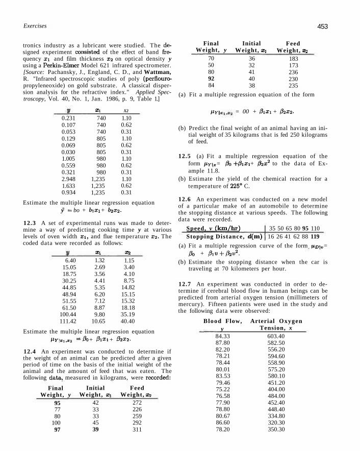
12.2 In Applied Spectroscopy, the infrared reflectance spectra properties of a viscous liquid used in the clec-
Exercises 453
tronics industry as a lubricant were studied. The designed experiment consisted of the effect of band frea-quency Xi and film thickness x2 on optical density y using a Perkin-Elmer Model 621 infrared spectrometer. [Source: Pachansky, J., England, C. D., and Wattman, R. "Infrared spectroscopic studies of poly (perflouro-propyleneoxide) on gold substrate. A classical dispersion analysis for the refractive index." Applied Spectroscopy, Vol. 40, No. 1, Jan. 1986, p. 9, Table 1.]
X i X2
0.231 0.107 0.053 0.129 0.069 0.030 1.005 0.559 0.321 2.948 1.633 0.934
740 740 740 805 805 805 980 980 980
1,235 1,235 1,235
1.10 0.62 0.31 1.10 0.62 0.31 1.10 0.62 0.31 1.10 0.62 0.31
Estimate the multiple linear regression equation y = bo + bixi + b2x2.
12.3 A set of experimental runs was made to determine a way of predicting cooking time y at various levels of oven width x i , and flue temperature x2. The coded data were recorded as follows:
X l X2
6.40 15.05 18.75 30.25 44.85 48.94 51.55 61.50
100.44 111.42
1.32 2.69 3.56 4.41 5.35 6.20 7.12 8.87 9.80
10.65
1.15 3.40 4.10 8.75
14.82 15.15 15.32 18.18 35.19 40.40
Estimate the multiple linear regression equation Myi^ ,^ =0o + 0\xi + 02X2.
12.4 An experiment was conducted to determine if the weight of an animal can be predicted after a given period of time on the basis of the initial weight of the animal and the amount of feed that was eaten. The following data, measured in kilograms, were recorded:
Final Weight, y
95 77 80
100 97
Initial Weight, xi
42 33 33 45 39
Feed Weight, X2
272 226 259 292 311
Final Weight, y
70 50 80 92 84
Initial Weight, Xi
36 32 41 40 38
Feed Weight, X2
183 173 236 230 235
(a) Fit a multiple regression equation of the form
PY\x = 00 + 0ixx + 02x2.
(b) Predict the final weight of an animal having an initial weight of 35 kilograms that is fed 250 kilograms of feed.
12.5 (a) Fit a multiple regression equation of the form pY\x = 0Q+ 0m + 0\x2 to the data of Example 11.8.
(b) Estimate the yield of the chemical reaction for a temperature of 225° C.
12.6 An experiment was conducted on a new model of a particular make of an automobile to determine the stopping distance at various speeds. The following data were recorded.
Speed, v (km/hr) 35 50 65 80 95 110 Stopping Distance, d(m) 16 26 41 62 88 119
(a) Fit a multiple regression curve of the form up\v = 0O + 0W+02V2.
(b) Estimate the stopping distance when the car is traveling at 70 kilometers per hour.
12.7 An experiment was conducted in order to determine if cerebral blood flow in human beings can be predicted from arterial oxygen tension (millimeters of mercury). Fifteen patients were used in the study and the following data were observed:
Blood Flow, y
84.33 87.80 82.20 78.21 78.44 80.01 83.53 79.46 75.22 76.58 77.90 78.80 80.67 86.60 78.20
Arterial Oxygen Tension, x
603.40 582.50 556.20 594.60 558.90 575.20 580.10 451.20 404.00 484.00 452.40 448.40 334.80 320.30 350.30

454 Chapter 12 Multiple Linear Regression and Certain Nonlinear Regression A4odels
Estimate the quadratic regression equation
PY\x = 3o + 0ix + 02X2.
12 .8 The following is a set of coded experimental data on the compressive strength of a particular alloy at various values of the concentration of some additive:
scores of four tests. The data are as follows:
Concentration, X
10.0 15.0 20.0 25.0 30.0
Compressive
25.2 29.8 31.2 31.7 29.4
Strength, y
27.3 28.7 31.1 27.8 32.6 29.7 30.1 32.3 30.8 32.8
(a) Estimate the quadratic regression equation py\x = 0o + 0iX + p\x2.
(b) Test for lack of fit of the model.
12.9 The electric power consumed each month by a chemical plant is thought to be related to the average ambient temperature x i , the number of days in the month x2, the average product purity X3, and the tons of product produced X4. The past year's historical data are available and are presented in the following table.
X ] X2 ak X ]
240 236 290 274 301 316 300 296 267 276 288 261
25 31 45 60 65 72 80 84 75 60 50 38
24 21 24 25 25 26 25 25 24 25 25 23
91 90 88 87 91 94 87 86 88 91 90 89
100 95 110 88 94 99 97 96 110 105 100 98
(a) Fit a multiple linear regression model using the above data set.
(b) Predict power consumption for a month in which xi = 75°F, x2 = 24 days, x3 = 90%, and x4 = 98 tons.
12.10 Given the data
X
y
0 l
l 4
2 5
3 3
4 2
5 3
6 4
(a) Fit the cubic model fiy\x = 30 +0ix+02x2 + 03x*.
(b) Predict Y when x = 2.
12.11 The personnel department of a certain industrial firm used 12 subjects in a study to determine the relationship between job performance rating (y) and
y Xl X2 X.]
11.2 14.5 17.2 17.8 19.3 24.5 21.2 16.9 14.8 20.0 13.2 22.5
56.5 59.5 69.2 74.5 81.2 88.0 78.2 69.0 58.1 80.5 58.3 84.0
71.0 72.5 76.0 79.5 84.0 86.2 80.5 72.0 68.0 85.0 71.0 87.2
38.5 38.2 42.5 43.4 47.5 47.4 44.5 41.8 42.1 48.1 37.5 51.0
43.0 44.8 49.0 56.3 60.2 62.0 58.1 48.1 46.0 60.3 47.1 65.2
Estimate the regression coefficients in the model
y = bo + bixi + b2x2 + b3x3 + &4X4.
12.12 The following data reflect information taken from 17 U.S. Naval hospitals at various sites around the world. The regressors are workload variables, that is, items that result in the need for personnel in a hospital installation. A brief description of the variables is as follows:
y = monthly labor-hours,
xi = average daily patient load,
X2 = monthly X-ray exposures,
X3 = monthly occupied bed-days,
X4 = eligible population in the area/1000,
i s = average length of patient's stay, in days.
Site xi X2 X3 Xl X 5 y 1 2 3 4 5 6 7 8 9 10 11 12 13 14 15 16 17
15.57 44.02 20.42 18.74 49.20 44.92 55.48 59.28 94.39 128.02 96.00 131.42 127.21 252.90 409.20 463.70 510.22
2463 2048 3940 6505 5723 11520 5779 5969 8461
20106 13313 10771 15543 36194 34703 39204 86533
472.92 1339.75 620.25 568.33 1497.60 1365.83 1687.00 1639.92 2872.33 3655.08 2912.00 3921.00 3865.67 7684.10
12446.33 14098.40 15524.00
18.0 9.5 12.8 36.7 35.7 24.0 43.3 46.7 78.7 180.5 60.9 103.7 126.8 157.7 169.4 331.4 371.6
4.45 6.92 4.28 3.90 5.50 4.60 5.62 5.15 6.18 6.15 5.88 4.88 5.50 7.00 10.75 7.05 6.35
566.52 696.82 1033.15 1003.62 1611.37 1613.27 1854.17 2160.55 2305.58 3503.93 3571.59 3741.40 4026.52 10343.81 11732.17 15414.94 18854.45
The goal here is to produce an empirical equation that will estimate (or predict) personnel needs for Naval hospitals. Estimate the multiple linear regression equa-

Exercises 455
tion
PY\xi,X2.X3,I4,x$
= 00 + 0Hl + 02X2 + 03X3 + 0AXI + 05X5-
12.13 An experiment was conducted to study the size of squid eaten by sharks and tuna. The regressor variables are characteristics of the beak or mouth of the squid. The regressor variables and response considered for the study are
xi = rostral length, in inches,
x2 = wing length, in inches,
X3 = rostral to notch length, in inches,
X4 = notch to wing length, in inches,
X5 = width, in inches,
y = weight, in pounds.
Xl X 2 X3 X4
Xl X2 X3 X4 Xs y 1.31 1.55 0.99 0.99 1.01 1.09 1.08 1.27 0.99 1.34 1.30 1.33 1.86 1.58 1.97 1.80 1.75 1.72 1.68 1.75 2.19 1.73
1.07 1.49 0.84 0.83 0.90 0.93 0.90 1.08 0.85 1.13 1.10 1.10 1.47 1.34 1.59 1.56 1.58 1.43 1.57 1.59 1.86 1.67
0.44 0.53 0.34 0.34 0.36 0.42 0.40 0.44 0.36 0.45 0.45 0.48 0.60 0.52 0.67 0.66 0.63 0.64 0.72 0.68 0.75 0.64
0.75 0.90 0.57 0.54 0.64 0.61 0.51 0.77 0.56 0.77 0.76 0.77 1.01 0.95 1.20 1.02 1.09 1.02 0.96 1.08 1.24 1.14
0.35 0.47 0.32 0.27 0.30 0.31 0.31 0.34 0.29 0.37 0.38 0.38 0.65 0.50 0.59 0.59 0.59 0.63 0.68 0.62 0.72 0.55
1.95 2.90 0.72 0.81 1.09 1.22 1.02 1.93 0.64 2.08 1.98 1.90 8.56 4.49 8.49 6.17 7.54 6.36 7.63 7.78
10.15 6.88
410 569 425 344 324 505 235 501 400 584 434
late the
69 57 77 81
0 53 77 76 65 97 76
multiple
125 131 141 122 141 152 141 132 157 166 141
linear
59.00 31.75 80.50 75.00 49.00 49.35 60.75 41.25 50.75 32.25 54.50
55.66 63.97 45.32 46.67 41.21 43.83 41.61 64.57 42.41 57.95 57.90
regression equation
f*Y\ X\ ,X2,X\1 P^4 00 + /3lXl + 02X2 + /33X3 + 04X4.
12.15 A study was performed on wear of a bearing y and its relationship to xi = oil viscosity and X2 = load. The following data were obtained. [Prom Response Surface Methodology, Myers and Montgomery (2002).]
y Xl X2 y Xl X2
193 172 113
1.6 22.0 33.0
851 1058 1357
230 91
125
15.5 43.0 40.0
816 1201 1115
Estimate the multiple linear regression equation
l^Y\x\ ,X2IX3,X4,25
= 00 + 3\Xl + 02X2 + 03X3 + /?4Xl + 05X5.
12.14 Twenty-three student teachers took part in an evaluation program designed to measure teacher effectiveness and determine what factors are important. Eleven female instructors took part. The response measure was a quantitative evaluation made on the cooperating teacher. The regressor variables were scores on four standardized tests given to each instructor. The data are as follows:
(a) Estimate the unknown parameters of the multiple linear regression equation
f.Y\xi,x2 =00+ 0\X\ +02X2-
(b) Predict wear when oil viscosity is 20 and load is 1200.
12.16 An engineer at a semiconductor company wants to model the relationship between the device gain or hFE(y) and three parameters: emitter-RS (xi), base-RS (X2), and emitter-to-base-RS (X3). The data are shown below:
X i , X2, X3, y , Emitter-RS cBase-RS E-B-RS h F E - l M - 5 V
14.62 15.63 14.62 15.00 14.50 15.25 16.12 15.13 15.50 15.13 15.50 16.12 15.13 15.63 15.38 15.50
226.0 220.0 217.4 220.0 226.5 224.1 220.5 223.5 217.6 228.5 230.2 226.5 226.6 225.6 234.0 230.0
7.000 3.375 6.375 6.000 7.625 6.000 3.375 6.125 5.000 6.625 5.750 3.750 6.125 5.375 8.875 4.000
128.40 52.62
113.90 98.01
139.90 102.60 48.14
109.60 82.68
112.60 97.52 59.06
111,80 89.09
171.90 66.80

456 Chapter 12 Multiple Linear Regression and Certain Nonlinear Regression. Models
xi, x2, x3, y, Emitter-RS cBase-RS E-B-RS hFE-lM-5V
14.25 14.50 14.62
224.3 240.5 223.7
8.000 10.870 7.375
157.11) 208.40 133.40
(a) Fit a multiple linear regression to the data. (b) Predict hFE when x3 = 14. x2 = 220, and i::i
[Data from Myers and Montgomery (2002)].
12.4 Properties of the Least Squares Estimators
The means and variances of the estimators bo, bx,..., bk are readily obtained under certain assumptions on the random errors ej, e2,..., ck that are identical to those made in the case of simple linear regression. When we assume these errors to be independent, each with zero mean and variance er", it can then be shown that bo,b\,... ,bk arc. respectively, unbiased estimators of the regression coefficients 0o, 0x, • • • ,3k- In addition, the variances of b's are obtained through the elements of the inverse of the A matrix. Note that the off-diagonal elements of A = X'X represent sums of products of elements in the columns of X, while the diagonal elements of A represent sums of squares of elements in the columns of X. The inverse matrix, A - 1 , apart from the multiplier a2, represents the variance-covariance mat r ix of the estimated regression coefficients. That is, the elements of the matrix A_1er display the variances of bo, b], . . . , bk on the main diagonal and covariances on the off-diagonal. For example, in a A- = 2 multiple linear regression problem, we might write
(X'X)-
with the elements below the main diagonal determined through the symmetry of the matrix. Then we can write
of. = cao2, i = 0,1,2,
Ob^bj = Cov(bi,bj)= CijO2, i ^ j .
Of course, the estimates of the variances and hence flic standard errors of these estimators are obtained by replacing er2 with the appropriate estimate obtained through experimental data. An unbiased estimate of a2 is once again defined in terms of the error stun of squares, which is computed using the formula established in Theorem 12.1. In the theorem we are making the assumptions on the e-, described above.
coo ClO
C20
CQl
C - l l
cai
C02
Cl2
C22
Theorem 12.1: Fo
an
r the linear regression
unbiased estimate of o
2 8 =
SSE n - k - l
equation
y =
2 is given
where
X3 +
by the
SSE--
e,
error
n
=£ ?:=i
or
el
residual
= £> i = i
mean
-Vi?
sepi ire
We can see that Theorem 12.1 represents a generalization of Theorem 11.1

12.4 Properties of the Least Squares Estimators 457
for the simple linear regression case. The proof is left for the reader. As in the simpler linear regression case, the estimate s2 is a measure of the variation in the prediction errors or residuals. Other important inferences regarding the fitted regression equation, based on the values of the individual residuals e^ = yi — yi, i = l , 2 , . . . , n, are discussed in Sections 12.10 and 12.11.
The error and regression sum of squares take on the same form and play the same role as in the simple linear regression case. In fact, the sum-of-squares identity
£ > " V? = £ > - V? + f > - Vi? i—l 2 = 1 ;'.= 1
continues to hold and wc retain our previous notation, namely,
SST = SSR + SSE
with
n
SST = 2_,iy> ~ y? = t'0*8-! s u m OI squares, i = i
and
SSR = ^Jfj/i — y? = regression sum of squares. ; = i
There are A; degrees of freedom associated with SSR and, as always, SST has n — 1 degrees of freedom. Therefore, after subtraction, SSE has n — k — 1 degrees of freedom. Thus our estimate of er2 is again given by the error sum of squares divided by its degrees of freedom. All three of these sums of squares will appear on the printout of most multiple regression computer packages.
Analysis of Variance in Mult iple Regression
The partition of total sum of squares into its components, the regression and error sum of squares, plays an important role. An analysis of variance can be conducted that sheds light on the quality of the regression equation. A useful hypothesis that determines if a significant amount of variation is explained by the model is
#o : 0i = 02 = 1% = •• • = 0k = 0.
The analysis of variance involves an F-test via a table given as follows:
Source
Regression
Error
Total
Sum of Squares
SSR
SSE
SST
Degrees of Freedom
k
n-(k+l)
n - 1
Mean Squares
MSR = ^f2
HfQf? SSE MSL - n _ ( f c + 1 )
F f _ MSR •> MSE

458 Chapter 12 Multiple Linear Regression and Certain Nonlinear Regression Models
The test involved is an upper-tailed test. Rejection of H0 implies that the regression equation differs from a constant. That is, at least one regressor variable is important. Further discussion of the use of analysis of variance appears in subsequent sections.
Further utility of the mean square error (or residual mean square) lies in its use in hypothesis testing and confidence interval estimation, which is discussed in Section 12.5. In addition, the mean square error plays an important role in situations where the scientist is searching for the best from a set of competing models. Many model-building criteria involve the statistic s2. Criteria for comparing competing models are discussed in Section 12.11.
12.5 Inferences in Multiple Linear Regression
One of the most useful inferences that can be made regarding the quality of the predicted response yo corresponding to the values arm, X2Q, ..., Xko is the confidence interval on the mean response py\Xw,x.Jt Xka- We are interested in constructing a confidence interval on the mean response for the set of conditions given by
xo = [1,xio,X2ot •••-.Xka}-
We augment the conditions on the x's by the number 1 in order to facilitate the matrix notation. Normality in the £{ produces normality in the bjS and the mean, variances, and covariances are still the same as indicated in Section 12.4. Hence
k
y - b°+YI bJxj° J = I
is likewise normally distributed and is, in fact, an unbiased estimator for the mean response on which we are attempting to attach confidence intervals. The variance of yo, written in matrix notation simply as a function of cr2, ( X ' X ) - 1 , and the condition vector Xrj, is
0$, = c72x(J(X'X)-1x0.
If this expression is expanded for a given case, say k = 2, it is readily seen that it appropriately accounts for the variances and covariances of the ft/s. After replacing er2 by s2 as given by Theorem 12.1, the 100(1 — a)% confidence interval on Mv|a;io.x2o....,2to c a n oe constructed from the statistic
rp _ VO — llY\x,0,X20,--,Xk0
Vxd(X'X)-1x0 '
which has a i-distribution with n — k — 1 degrees of freedom.
Confidence Interval A 100(1 — a)% confidence interval for the mean response py\xm_, for PY\xla,xm,...,Xk0
2/0 - iQ/2S\/x6(X'X)-1Xo < PY\xw,xM,...,xku <V0 + ta/2Sy/x6(X'X)-lK0,
where ta/2 is a value of the ^-distribution with n — k — 1 degrees of freedom.

22.5 Inferences in Multiple Linear Regression 459
The quantity sy'x<5(X'X)~1x0 is often called the standard error of prediction and usually appears on the printout of many regression computer packages.
Example 12.5:1 Using the data of Example 12.3, construct a 95% confidence interval for the mean response when xx = 3%. x2 = 8%, and x3 = 9%.
Solution: From the regression equation of Example 12.3, the estimated percent survival when xx = 3%, x2 = 8%, and x3 = 9% is
y = 39.1574+ (1.0161)(3) - (1.8616)(8) - (0.3433)(9) = 24.2232.
Next we find that
x 0(X'X)-1x 0 = [1,3,8,9]
8.0648 -0.0826 -0.0942 -0.7905 -0.0826 0.0085 0.0017 0.0037 -0,0942 0.0017 0.0166 -0.0021 -0.7905 0.0037 -0.0021 0.0886
= 0.1267.
Using the mean square error, s2 = 4.298 or s = 2.073, and Table A.4, we see that £0.025 = 2.262 for 9 degrees of freedom. Therefore, a 95% confidence interval for the mean percent survival for xx = 3%, x2 = 8%, and X3 = 9% is given by
24.2232 - (2.262)(2.073)\/0.1267 < py\3,s,c,
< 24.2232 + (2.262)(2.073)V0.1267,
or simply 22.5541 < MV|3,8,9 < 25.8923. J As in the case of simple linear regression, we need to make a clear distinction
between the confidence interval on a mean response and the prediction interval on an observed response. The latter provides a bound within which we can say with a preselected degree of certainty that a new observed response will fall.
A prediction interval for a single predicted response yo is once again established by considering the difference y0 — y0. The sampling distribution can be shown to be normal with mean
^Oo-yo ~ 0,
and variance
<£-*,» ^[l + xftX'X)-1*,].
Thus a 100(1 - a)% prediction interval for a single prediction value yo can be constructed from the statistic
T = Vo -yo Sy/l + x6(X'X)-W
which has a t-distribution with n — k — 1 degrees of freedom.

460 Chapter 12 Multiple Linear Regression and Certain Nonlinear Regression Models
Prediction Interval A 100(1 — a)% prediction interval for a single response i/o is given by for j/o
2/0 " <Q/2*\/l+X($(X'X)-1Xo < 2/0 < VO + ta/2SV'l + X<J(X'X)-1Xo>
where ta/2 is a value of the t-distribution with n — k — 1 degrees of freedom.
Example 12.6:1 Using the data of Example 12.3, construct a 95% prediction interval for an individual percent survival response when xx = 3%, x2 = 8%, and x3 = 9%.
Solution: Referring to the results of Example 12.5, we find that the 95% prediction interval for the response yo, when xx = 3%, x2 = 8%., and X3 = 9%, is
24.2232 - (2.262)(2.073)\/1.1267 <y0< 24.2232
+ (2.262)(2.073)\/l.l267,
which reduces to 19.2459 < 2/0 < 29.2005. Notice, as expected, that the prediction interval is considerably wider than the confidence interval for mean percent survival in Example 12.5. J
A knowledge of the distributions of the individual coefficient estimators enables the experimenter to construct confidence intervals for the coefficients and to test hypotheses about them. Recall from Section 12.4 that the b,'s (j = 0,1,2,.. ,,k) are normally distributed with mean 0j and variance Cjja2. Thus we can use the statistic
t = _ bj - 0jp
s./c 33
with n — k — I degrees of freedom to test hypotheses and construct confidence intervals on 0j. For example, if we wish to test
#0: 0j = 0jo> Hi'. 0j ^ 0JO,
we compute the above i-statistic and do not reject HQ if -ta/2 < t < ta/2, where taj2 has n — k — 1 degrees of freedom.
Example 12.7:1 For the model of Example 12.3, test the hypothesis that 02 = -2 .5 at the 0.05 level of significance against the alternative that 02 > —2.5.
Solution: H0: 02 = -2 .5 ,
Hi: 32 > -2 .5 .
Computations:
t = b2 - 02O = -1-8616 + 2.5 = 2 3 g o
sy/c^ 2.073 VQ.0166 ' '
P = P(T > 2.390) = 0.04.
Decision: Reject Ho and conclude that 02 > —2.5.

12.5 Inferences in Multiple Linear Regression 461
Individual T-Tests for Variable Screening
The i-tcst most often used in multiple regression is the one which tests the importance of individual coefficients (i.e., H$j — 0 against the alternative Hi: 0j ^ 0). These tests often contribute to what is termed variable screening where the analyst attempts to arrive at the most useful model (i.e., the choice of wdiich regressors to use). It should be emphasized here that if a coefficient is found insignificant (i.e., the hypothesis H0: 0j = 0 is not rejected), the conclusion drawn is that the variable is insignificant (i.e., explains an insignificant amount, of variation in y), in the presence of the other regressors in the model. This point will be reaffirmed in a future discussion.
Annotated Printout for Data of Example 12.3
Figure 12.1 shows an annotated computer printout for a multiple linear regression fit to the data of Example 12.3. The package used is 5.45.
Note the model parameter estimates, the standard errors, and the i-statistics shown in the output. The standard errors are computed from square roots of diagonal elements of (X'X)~1s2. In this illustration the variable x3 is insignificant in the presence of xx and x2 based on the i-test and the corresponding P-value = 0.5916. The terms CLM and CLI are confidence intervals on mean response and prediction limits on an individual observation, respectively. The /-test in the analysis of variance indicates that a significant amount of variability is explained. As an example of the interpretation of CLM and CLI, consider observation 10. With an observation of 25.2 and a predicted value of 26.068, we are 95% confident that the mean response is between 24.502 and 27.633, and a new observation will fall between 21.124 and 31.011 with probability 0.95. The R2 value of 0.9117 implies that the model explains 91.17% of the variability in the response. More discussion about i£2-appears in Section 12.6.
More on Analysis of Variance in Multiple Regression (Optional)
In Section 12.4 we discussed briefly the partition of the total sum of squares
YI iVi — 'V? m t ° its two components, the regression model and error sums of squares »=i (illustrated in Figure 12.1). The analysis of variance leads to a test of
Ho: 0i=02=03 = --- = 0k = 0.
Rejection of the null hypothesis has an important interpretation for the scientist or engineer. (For those who are interested in more treatment of the subject using matrices, it is useful to discuss the development of these sums of squares used in ANOVA.)
First recall from the definition of y, X, and 0 in Section 12.3, as well as b, the vector of least squares estimators given by
b = (X'X) - ' X ' y .

462 Chapter 12 Multiple Linear Regression and Certain Nonlinear Regression Models
Source
Model
Error
Corrected Total
Root MSE Dependent Mean
Coeff Var
Variable DF
Intercept 1
xl x2 x3
1 1 1
Sum of Mean
DF Squares Square F Value Pr >
3 399.45437 133.:
F 15146 30.98 <.0001
9 38.67640 4.29738
12 438.13077
2.07301 R-Square
29.03846 Adj R-Sq
7.13885
Parameter
Estimate
39.15735
1.01610
-1.86165
-0.34326
Dependent Predicted Std Error
Obs 1 2 3 4 5 6 7 8 9 10 11 12 13
Variable
25.5000
31.2000
25.9000
38.4000
18.4000
26.7000
26.4000
25.9000
32.0000
25.2000
39.7000
35.7000
26.5000
Value Mean Predict
27.3514 1.4152
32.2623 0.7846
27.3495 1.3588
38.3096 1.2818
15.5447 1.5789
26.1081 1.0358
28.2532 0.8094
26.2219 0.9732
32.0882 0.7828
26.0676 0.6919
37.2524 1.3070
32.4879 1.4648
28.2032 0.9841
0.9117
0.8823
Standard
Error
5.88706
0.19090
0.26733
0.61705
95'/. CL
24.1500
30.4875
24.2757
35.4099
11.9730
23.7649
26.4222
24.0204
30.3175
24.5024
34.2957
29.1743
25.9771
t Value
6.65
5.32
-6.96
-0.56
Mean
30.5528
34.0371
30.4234
41.2093
19.1165
28.4512
30.0841
28.4233
33.8589
27.6329
40.2090
35.8015
30.4294
Pr > Itl <,0001
0.0005
<.0001
0.5916
95'/, CL
21 27 21 32 9 20 23 21 27 21 31 26 23
.6734
.2482
.7425
.7960
.6499
.8658
.2189
.0414
.0755
.1238
.7086
.7459
.0122
Predict
33.0294
37.2764
32.9566
43.8232
21.4395
31.3503
33.2874
31.4023
37.1008
31.0114
42.7961
38.2300
33.3943
Residual
-1.8514
-1.0623
-1.4495
0.0904
2.8553
0.5919
-1.8532
-0.3219
-0.0882
-0.8676
2.4476
3.2121
-1.7032
Figure 12.1: 5.45 printout for data in Example 12.3.
A partition of the uncorrected sum of squares
y'y = X>2 j = i
into two components is given by
y'y = b 'X 'y + (y'y - b 'X'y)
= y 'X(X 'X) - 1 X'y + [y'y - y 'X(X 'X) - l X'y] .
The second term (in brackets) on the right-hand side is simply the error sum of n
squares Y2 iVi —Vi)2- The reader should see that an alternative expression for the ; = i
error sum of squares is
SSE = y'[I„ - X(X'X)-1X']y.

12.5 Inferences in Multiple Linear Regression 463
The term y ' X ( X ' X ) - X'y is called the regression sum of squares. However, n
it is not the expression YI iVi ~ V? used for testing the "importance" of the terms i=[
bx, b2,..., bk but, rather,
y'X(X'XrxX'y = I>? 2 i >
i = l
which is a regression sum of squares uncorrected for the mean. As such it would only be used in testing if the "regression equation differs significantly from zero." That is,
H0: 0o=0i=02 = ---=0k = 0.
In general, this is not as important as testing
HQ: 0i=02 = --- = 0k = 0,
since the latter states that the mean response is a constant, not necessarily zero.
Degrees of Freedom
Thus the partition of sums of squares and degrees of freedom reduces to
Source Sum of Squares d.f.
Regression £ y2 = y ' X ( X ' X ) - 1 X ' y fe + 1 i-l
Error YZilH ~ m? = y'fc. - X(X'X)- 1 X']y n-(k + 1) i = l
Total £ yf = y'y n i = l
Hypothesis of Interest
Now, of course, the hypotheses of interest for an ANOVA must eliminate the role of the intercept in that described previously. Strictly speaking, if Ho : 0x = 02 = • • • — 0k — 0, then the estimated regression line is merely y; = y. As a result, we are actually seeking evidence that the regression equation "varies from a constant." Thus, the total and regression sums of squares must be "corrected for the mean." As a result, we have
;=1 i = l i = l
In matrix notation this is simply
y ' [In - l f l ' l V ^ l ' l y = y ' [ X ( X ' X ) - 1 X ' - l f l ' l j - ^ y
+ y ' ( I „ - X ( X ' X ) - 1 X ' ] y .

464 Chapter 12 Multiple Linear Regression and Certain Nonlinear Regression Models
In this expression 1 is merely a vector of n ones. As a result, we are merely subtracting
y ' l ( l ' l ) - 1 l ' y = i ^ ^ )
from y 'y and from y 'X(X 'X) _ 1 X'y (i.e., correcting the total and regression sum of squares for the mean).
Finally, the appropriate partitioning of sums of squares with degrees of freedom is as follows:
Source Sum of Squares d.f.
Regression £ (ft - y)2 = y T X f X ' X ) - ^ ' - l ( l ' l ) - 1 l ] y k i=i
Error £ (yt - y{)2 = y '[In - X(X'X)" 1 X']y n - (k + 1)
1=1
Total £ ( 2 / i -y ) 2 =y ' [ I n - l ( l / l ) - 1 l ' ] y n - 1 i=\
This is the ANOVA table that appears in the computer printout of Figure 12.1. The expression y ' [ l ( l ' l ) - 1 l ' ] y is often called the regression sum of squares associated with the mean, and 1 degree of freedom is allocated to it.
Exercises
12.17 For the data of Exercise 12.2 on page 452, es- confidence interval for the mean compressive strength timate a2. when the concentration is x = 19.5 and a quadratic
model is used. 12.18 For the data of Exercise 12.3 on page 453, estimate a2. 12.24 Using the data of Exercise 12.9 on page 454
and the estimate of a2 from Exercise 12.19, compute 12.19 For the data of Exercise 12.9 on page 454, es- 95% confidence intervals for the predicted response and timate a . the mean response when xi = 75, x2 = 24, x3 = 90,
and X4 = 98. 12.20 Obtain estimates of the variances and the co-variance of the estimators bx and b2 of Exercise 12.2 on 1 2 . 2 5 For the model of Exercise 12.7 on page 453, page 452. t e s t t h e hypothesis that 02 = 0 at the 0.05 level of
significance against the alternative that 02 ^ 0. 12.21 Referring to Exercise 12.9 on page 454, find the estimate of 1 2 . 2 6 For the model of Exercise 12.2 on page 452, (a) a2
2, test the hypothesis that 0i = 0 at the 0.05 level of (b) Cov(bi 64). significance against the alternative that 0i / 0,
, . . , „ , i U , . r „ ,„ . . , . 1 2 . 2 7 For the model of Exercise 12.3 on page 453, 12.22 Using the data of Exercise 12.2 on page 452 . . .. , ., .. . a „ . . ., ,. .<.•
j .1. ... j. e 2c -^ • -in,-. test the hypotheses that 3\ = 2 against the alternative and the estimate of er" from Exercise 12.17. compute ,, , 0 ,,„„ „ D , „,„„ . „ „ . „„„„,„• „ r n r „ , . t , , , ,. t , K , pi * 2. Use a /•'-value in your conclusion. 95% confidence intervals for the predicted response and ' the mean response when xi = 900 and x2 = 1.00. 1 2 2 8 Q ^ ^ t h e f o l l o w i n g d a U t h a t ig l i s t e d f a
„ „ . „ „ ,_ . -, Exercise 12.15 on page 455. 12.23 For Exercise 12.8 on page 4o4, construct a 90% H b

y (wear) 193 230 172 91
113 125
Xi ( o 1 viscosii 1.6
15.5 22.0 43.0 33.0 40.0
ty) x< (load) 851 816
1058 1201 1357 1115
12.6 Choice of a Fitted Model through Hypothesis Testing 465
(a) Ho: 01 = 0 versus // , : 3i # 0; (b) H0: 02 = 0 versus Hi: 32 5* 0. (c) Do you have any reason to believe that the model
in Exercise 12.28 should be changed? Why or win-not?
, , , - , , . 2 ... , , 12.30 Using the data from Exercise 12.16 on page (aj Estimate er using multiple regression of y on ;r:i . r ,
and x2. ' „ ,, , „ ,. , , „,fw „ , . . (a) Estimate o using the multiple regression of y on ID) Compute predicted values, a 95% confidence; inter- , , e i n,n/ i- • i xi. Xi. and 2:3:
val tor mean wear, and a 95% prediction interval for observed wear if xi = 20 and x2 = 1000. (u) Compute a 95%. prediction interval for the observed
device gain for the three regressors tit Xi = 15.0, 12.29 Using the data from Exercise 12.28, teat, tit. X2 = 2 2 0 ' 0 ' a i l d x* = 6*0,
level 0.05
12.6 Choice of a Fitted Model Through Hypothesis Testing
In many regression situations, individual coefficients are of importance to the experimenter. For example, in an economics application, 0x,p\, • • • might have some particular significance, and thus confidence intervals and tests of hypotheses on these parameters are of interest to the economist. However, consider an industrial chemical situation in which the postulated model assumes that reaction yield is dependent linearly on reaction temperature and concentration of a certain catalyst. It is probably known that this is not the true model but an adequate approximation, so the interest is likely not to be in the individual parameters but rather in the ability of the entire function to predict the true response in the range of the variables considered. Therefore, in this situation, one would put more emphasis on er? confidence intervals on the mean response, and so forth, and likely deemphasize inferences on individual parameters.
The experimenter using regression analysis is also interested in deletion of variables when the situation dictates that, in addition to arriving at a workable prediction equation, he or she: must find the ''best regression" involving only variables that are useful predictors. There are a number of available computer programs that sequentially arrive at the so-called best regression equation depending on certain criteria. We discuss this further in Section 12.9.
One criterion that is commonly used to illustrate the adequacy of a fitted regression model is the coefficient of mult iple de te rmina t ion :
SSR g ,<» ' - T J ) 2 SSE
" « " • " £ < » - « • " ~ s s r
/ - - 1
Note tha t this parallels the description of R2 in Chapter 11. At this point the explanation might be more clear since we now focus on SSR. as the v a r i a b i l i t y e x p l a i n e d . The quanti ty R2 merely indicates what proportion of the total variation in the response Y is explained by the fitted model. Often an experimenter will report R2 x 100% and interpret the result as percentage variation explained by

466 Chapter 12 Multiple Linear Regression and Certain Nonlinear Regression Models
the postulated model. The square root of R2 is called the multiple correlation coefficient between Kand the set x\,x2,..., Xk- In Example 12.3, the value of R2
indicating the proportion of variation explained by the three independent variables Xi, x2, and x3 is found to be
55H = 399:45 = 1 SST 438.13 J
which means that 91.17% of the variation in percent survival has been explained by the linear regression model.
The regression sum of squares can be used to give some indication concerning whether or not the model is an adequate explanation of the true situation. We can test the hypothesis HQ that the regression is not significant by merely forming the ratio
SSR/k SSR/k } ~ SSE/{n-k-\)~ s2
and rejecting Ho at the a-level of significance when / > fa{k, n — k — 1). For the data of Example 12.3 we obtain
' 4.298
From the printout of Figure 12.1 the P-value is less than 0.0001. This should not be misinterpreted. Although it does indicate that the regression explained by the model is significant, this does not rule out the possibility that
1. The linear regression model in this set of x's is not the only model that can be used to explain the data; indeed, there may be other models with transformations on the x's that may give a larger value of the F-statistic.
2. The model may have been more effective with the inclusion of other variables in addition to Xi, x2, and x3 or perhaps with the deletion of one or more of the variables in the model, say x3, which displays P = 0.5916.
The reader should recall the discussion in Section 11.5 regarding the pitfalls in the use of R2 as a criterion for comparing competing models. These pitfalls are certainly relevant in multiple linear regression. In fact, the dangers in its employment in multiple regression are even more pronounced since the temptation to overfit is so great. One should always keep in mind the fact an R? « 1.0 can always be achieved at the expense of error degrees of freedom when an excess of model terms is employed. However, an R2 = 1, describing a model with a near perfect fit, does not always result in a model that predicts well.
The Adjusted Coefficient of Determination (Adjusted R2)
In Chapter 11 several figures displaying computer printout from both SAS and MINITAB featured a statistic called adjusted R? or adjusted coefficient of determination. Adjusted R? is a variation on R? that provides an adjustment for degrees of freedom. The coefficient of determination as defined on page 407 cannot decrease as terms are added to the model. In other words. R2 does not

12.6 Choice of a Fitted Model through Hypothesis Testing 467
decrease as the error degrees of freedom n — A: — 1 are reduced, the latter result being produced by an increase in k, the number of model terms. Adjusted R2
is computed by dividing SSE and SST by their respective values of degrees of freedom (i.e., adjusted R2 is as follows).
Adlui i idP? SSE/jn-k-1) adj SST/(n-l) '
To illustrate the use of R2d<, Example 12.3 is revisited.
How Are R2 and i?^dj Affected by Removal of a;3?
The t (or corresponding F) test for £3, the weight percent of ingredient 3, would certainly suggest that a simpler model involving only Xx and x2 may well be an improvement. In other words, the complete model with all the regressors maybe an overfitted model. It is certainly of interest to investigate R2 and R2
dt for both the full (xx,x2,x3) and restricted (x\,x2) models. We already know that HfM = 0.9117 by Figure 12.1. The SSE for the reduced model is 40.01 and thus ^restricted = 1 — .i38°i3 = 0-9087. Thus more variability is explained with 2:3 in the model. However, as wre have indicated, this will occur even if the model is an overfitted model. Now, of course, R\Ai is designed to provide a statistic that punishes an overfitted model so we might expect to favor the restricted model. Indeed, for the full model
2 38.6764/9 4.2974 K»d> - l ~ 438.1308/12 " l ~ 3U5109 " °M26,
whereas for the reduced model (deletion of x3)
2 40.01/10 4.001 n o n n i R°*> = * " 438.1308/12 = l ~ 36^109 = °-8 9°4-
Thus R2d- does indeed favor the restricted model and, indeed confirms the evidence
produced by the t- and F-tests that suggests that the reduced model is preferable to the model containing all three regressors. The reader may expect that other statistics may suggest the rejection of the overfitted model. See Exercise 12.40 on page 474.
Tests on Subsets and Individual Coefficients
The addition of any single variable to a regression system -will increase the regression sum squares and thus reduce the error sum of squares. Consequently, we must decide whether the increase in regression is sufficient to warrant using it in the model. As we might expect, the use of unimportant variables can reduce the effectiveness of the prediction equation by increasing the variable of the estimated response. We shall pursue this point further by considering the importance of £3 in Example 12.3. Initially, we can test
H0: 03 = O,
Hi: 03^O

468 Chapter 12 Multiple Linear Regression and Certain Nonlinear Regression Models
by using the (-distribution with 9 degrees of freedom. We have
6 3 - O -0.3433 t Sy/^sl 2.073v
/0l)886 -0.556,
which indicates that p\ does not differ significantly from zero, and hence we may very well feel justified in removing x3 from the model. Suppose that we consider the regression of y o n the set (xi,x2), the least squares normal equations now reducing to
13 59.43 81.82 59.43 394.7255 360.6621 81.82 360.6621 576.7264
bo 61 b2
=
377.50 1877.5670 2246.6610
The estimated regression coefficients for this reduced model are
/>o = 36.094, bx = 1.031, b2 = -1.870,
and the resulting regression sum of squares with 2 degrees of freedom is
Ri0i,02) = 398.12.
Here we use the notation R(0x,02) to indicate the regression sum of squares of the restricted model and it is not to be confused with SSR, the regression sum of squares of the original model with 3 degrees of freedom. The new error sum of squares is then
SST - R(0x,02) = 438.13 - 398.12 = 40.01,
and the resulting mean square error with 10 degrees of freedom becomes
, 40.01 10
= 4.001.
Does a Single Variable T-Test Have an JF Counterpar t?
The amount of variation in the response, the percent survival, which is attributed to x3, the weight percent of the third additive, in the presence of the variables xx and x2, is
Ri03\0\,02) = SSR - R(3i,02) = 399.45 - 398.12 = 1.33,
which represents a small proportion of the entire regression variation. This amount of added regression is statistically insignificant, as indicated by our previous test on 03. An equivalent test involves the formation of the ratio
/ RiM^M = 1-33
s2 4.298 0.309.
which is a value of the F-distribution with 1 and 9 degrees of freedom. Recall that the basic relationship between the (-distribution with v degrees of freedom and the F-distribution with 1 and v degrees of freedom is
t2 = f(l,v),

12.7 Special Case of Orthogonality (Optional) 469
and we note that the /-value of 0.309 is indeed the: square of the (-value of —0.56. To generalize the concepts above, we can assess the work of an independent
variable ;r, in the general multiple linear regression model
/ ' >> , ,X3,...,Xk = 00 + 0lX\ + r- 0kXk
by observing the amount of regression attributed to Xi over and above tha t a t t r i bu t ed to the o ther variables, that is, the regression on Xi adjusted for the other variables. This is computed by subtracting the regression sum of squares for a model with x; removed from SSR. For example, we say that as] is assessed by-calculating
R{0i\02,0:i 0k) = SSR - R(02,3:i, ...,0k.),
where R(02Jh, • • • ,3k) is the regression sum of squares with p\xi removed from the model. To test, the hypothesis
HQ: 0I = 0.
Hi: 0i+ 0,
compute
R.(0i \32,0:i,...,0k) J _9 !
and compare it with / „ ( l , n - k — 1). In a similar manner we can test, for the significance of a set of the variables.
For example, to investigate simultaneously the importance of including x\ and x2
in the model, wc test the hypothesis
HQ: 3i — 02 = 0,
Hi'. 0i and 0\ are not both zero,
by computing
. [R.(0i,02\03-.04,-..:0k)}/2 [SSR-R(03,34,...,0k)}/2 J s2 ,s2
and comparing il with fa(2,n—k — l). The number of degrees of freedom associated with the numerator, in this case 2, equals the number of variables in the set being investigated.
12.7 Special Case of Orthogonality (Optional)
Prior to our original development of the general linear regression problem, the assumption was made that the independent variables arc measured without error and arc often controlled by the experimenter. Quite often they occur as a result of an elaborately designed experiment. In fact, wc can increase the effectiveness of the resulting prediction equation with the use of a suitable experimental plan.

470 Chapter 12 Multiple Linear Regression and Certain Nonlinear Regression Models
Suppose that we once again consider the X matrix as defined in Section 12.3. We can rewrite it to read
X = [ l ,X 1 (X2,. . . ,X k ] ,
where 1 represents a column of ones and Xj is a column vector representing the levels of Xj. If
XpXq = 0, for p + q,
the variables xv and xq are said to be orthogonal to each other. There are certain obvious advantages to having a completely orthogonal situation whereby x,Jxq = 0 for all possible p and q,p + q, and, in addition,
n
^ £ j i = 0 , j = l,2,...,k. i=l
The resulting X 'X is a diagonal matrix and the normal equations in Section 12.3 reduce to
nbo = \V^yi, t = i
n n
&i YI x i ' = ]L xuyu
i=X i=X
bkJ2Xli =YsXkiyi' i=l i=X
An important advantage is that one is easily able to partition SSR into single-degree-of-freedom components , each of which corresponds to the amount of variation in Y accounted for by a given controlled variable. In the orthogonal situation we can write
n n
SSR = ]T(& - y? = Y^ib° + bixu + •'• + hxki - b0)2
t = i i = i n n n
= b2YJx\i+blY,x22i + --- + b2
k^4i i=\ r= l i = l
= R(0i) + R(02) + • • • + R(0k)-
The quantity R(0i) is the amount of regression sum of squares associated with a model involving a single independent variable Xi.
To test simultaneously for the significance of a set of m variables in an orthogonal situation, the regression sum of squares becomes
R.(0X, 02, -•-, 0m\0m+l, 0m+2, • • • , 0k) = Ri0x) + Ri02) + •" + «(/?m),

12.7 Special Case of Orthogonality (Optional) 471
and thus we have the further simplification
R(0i\02,03,...,0k) = Ri0i)
when evaluating a single independent variable. Therefore, the contribution of a given variable or set of variables is essentially found by ignoring the other variables in the model. Independent evaluations of the worth of the individual variables are accomplished using analysis-of-variance techniques as given in Table 12.4. The total variation in the response is partitioned into single-degree-of-freedom components plus the error term with n — k — 1 degrees of freedom. Each computed /-value is used to test one of the hypotheses
HQ: 3i = 01 . _ . „ , Hi: A ' ^ O j ' - 1 ^ - - - ^ -
by comparing with the critical point fa(\,n — k — 1) or merely interpreting the F-value computed from the /-distribution.
Table 12.4: Analysis of Variance for Orthogonal Variables
Source of Variation
A
02
0k
Error
Total
Sum of Squares
Rifii)=b\t*2u i=X
Ri02) = b2±x2., i= l
RiM = b\±xl SSE
»50i = iJyy
Degrees of Freedom
1
1
1
n - k -
n - 1
1
Mean Square
R(9x)
R{02)
Ri0k) n2 _ SSE b ~ n-k-[
Computed /
R(fli) s2
R(32) >
8*
Example 12.8:1 Suppose that a scientist takes experimental data on the radius of a propellant grain Fas a function of powder temperature x\, extrusion rate x2, and die temperature x3. Fit a linear regression model for predicting grain radius, and determine the effectiveness of each variable in the model. The data are given in Table 12.5.
Solution: Note that each variable is controlled at two levels, and the experiment represents each of the eight possible combinations. The data on the independent variables are coded for convenience by means of the following formulas:
powder temperature — 170 X, = 20 '
extrusion rate — 18 x2 = - ,
die temperature — 235 X3 = 15 •

472 Chapter 12 Multiple Linear Regression and Certain Nonlinear Regression Models
Table 12.5: Data for Example 12.8
Grain Radius
82 93
114 124 111 129 157 164
Powder Temperature
150 190 150 150 190 190 150 190
(-1) (+1) (-1) (-1) (+1) (+1) (-1) (+1)
Extrusion Rate
12 12 24 12 24 12 24 24
(-1) (-1) (+1) (-1) (+1) (-1) (+1) (+1)
Die Temperature
220 (-1) 220 (-1) 220 (-1) 250 (+1) 220 (-1) 250 (+1) 250 (+1) 250 (+1)
The resulting levels of Xx, x2, and x3 take on the values -1 and +1 as indicated in the table of data. This particular experimental design affords the orthogonality that we are illustrating here. A more thorough treatment of this type of experimental layout is discussed in Chapter 15. The X matrix is
X =
1 - ] 1 1 1 - ] 1 -1 1 1 1 ] 1 - ] 1 1
[ - 1 I - 1 I 1 1 - 1 1 1 [ - 1 1 1 i 1
- 1 - 1 - 1
1 - 1
1 1 1
and the orthogonality conditions are readily verified. We can now compute coefficients
6° = 5 X > = 12L75' 6l = \ !>«» = T = 2-5' t = i ? ' = 1
3 2 =
8
YI x-aVi i=l 118
14.75.
8
2-i X'iiVi 1 _ .
so in terms of the coded variables, the prediction equation is
y = 121.75 +2.5 Xi + 14.75 x2 + 21.75 £3.
The analysis-of-variance Table 12.6 shows independent contributions to SSR for each variable. The results, when compared to the /o.05(l-4) critical point of 7.71, indicate that £1 does not contribute significantly at the 0.05 level, whereas variables £2 and £3 are significant. In this example the estimate for a2 is 23.1250. As for the single-independent-variable case, it is pointed out that this estimate does not solely contain experimental error variation unless the postulated model is correct. Otherwise, the estimate is "contaminated" by lack of fit in addition to pure

Exercises 473
Table 12.6: Analysis of Variance for Grain Radius Data
Source of Sum of Degrees of Mean Computed Variation Squares Freedom Square / P- Value
01
02
03 Error
Total
(2.5)2(8) = 50
(14.75)2(8) = 1740.50
(21.75)2(8) = 3784.50
92.5
5667.50
1
1
1
4
7
50
1740.50
3784.50
23.1250
2.16
75.26
163.65
0.2156
0.0010
0.0002
Exercises
error, and the lack of fit can be separated only if we obtain multiple experimental observations at the various (xi,x2,x3) combinations.
Since £i is not significant, it can simply be eliminated from the model without altering the effects of the other variables. Note that £2 and £3 both impact the grain radius in a positive fashion, with £3 being the more important factor based on the smallness of the P-value. J j
12.31 Compute and interpret the coefficient of multiple determination for the variables of Exercise 12.3 on page 453.
12.32 Test whether the regression explained by the model in Exercise 12.3 on page 453 is significant at the 0.01 level of significance.
12.33 Test whether the regression explained by the model in Exercise 12.9 on page 454 is significant at the 0.01 level of significance.
12.34 For the model of Exercise 12.11 on page 454, test the hypothesis
H0: 0i=0i= 0, Hy. 0i and 02 are not both zero.
12.35 Repeat Exercise 12.26 on page 464 using an F-statistic.
12.36 A small experiment was conducted to fit a multiple regression equation relating the yield y to temperature xi, reaction time x2, and concentration of one of the reactants 23. Two levels of each variable were chosen and measurements corresponding to the coded independent variables were recorded as follows:
y 7.6 8.4 9.2
10.3 9.8
11.1 10.2 12.6
Xl
—1
— 1 — 1
— 1
* 2
- 1 - 1
1 - 1
1 - 1
1 1
x3 - 1 - 1 - 1
1 - 1
1 1 1
(a) Using the coded variables, estimate the multiple linear regression equation
V-Ylxx 00 + 0\Xl + 82X2 + 03X3.
(b) Partition SSR, the regression sum of squares, into three single-degree-of-freedom components attributable to £1, X2, and x3, respectively. Show an analysis-of-variance table, indicating significance tests on each variable.
12.37 Consider the electric power data of Exercise 12.9 on page 454. Test Ho '• 0i = 02 = 0 making use of Ri0i, 32\03,04). Give a P-value, and draw conclusions.
12.38 Consider the data for Exercise 12.36. Compute the followings
R(0i\0o), R(0i\0o,02,03),
R(02\0o,3i), R(02\0o,0i,03),
R(03\3o,0l,02).

474 Chapter 12 Multiple Linear Regression and Certain Nonlinear Regression Models
Comment.
12.39 Consider the data of Exercise 11.63 on page 439. Fit a regression model using weight and drive ratio as explanatory variables. Compare this model with the SLR (simple linear regression) model using weight alone. Use R2, R2^j, and any I- (or F)-statistics you may need to compare the SLR with the multiple regression model.
12.40 Consider Example 12.3. Figure 12.1 on page 462 displays a SAS printout of an analysis of the model containing variables xi, x2, and £3. Focus on the confidence interval of the mean response fiy at the (xi,x2,x3) locations representing the 13 data points. Consider an item in the printout indicated by C.V. This is the coefficient of variation, which is defined by
C.V. = - • 100. y
where s = y/s^ is the root mean squared error. The coefficient of variation is often used as yet another criterion for comparing competing models. It is a scale-free quantity which expresses the estimate of a, namely s, as a percent of the average response y. In competition for the "best" among a group of competing models, one strives for the model with a "small" value of C.V. Do a regression analysis of the data set shown in Example 12.3 but eliminate x3. Compare the full (xi,x2,x3) model with the restricted model (a.-), x2) and focus on two criteria: (i) C.V.; (ii) the widths of the confidence intervals on fiy- For the second criterion you may want to use the average width. Comment.
12.41 Consider Example 12.4 on page 451. Compare the two competing models
First order: yi = 0o + 0ixu + 02x2i + £>,
Second order: j/j = 0o + 0ixu + 82x21
+ 0\\X2u + 822x\i + 0\2XliX2i + et.
Use i?adj in your comparison in addition to testing Ho : 0n = 022 = 0n = 0. In addition, use C.V. discussed in Exercise 12.40.
12.42 In Example 12.8 on page 471 a case is made for eliminating x\, powder temperature, from the model since the P-value based on the .F-test is 0.2154 while P-values for x2 and £3 are near zero.
(a) Reduce the model by eliminating xi, thereby producing a full and restricted (or reduced) model and compare them on the basis of R2
d}.
(b) Compare the full and restricted models using the width of the 95% prediction intervals on a new observation. The "best" of the two models would be that with the "tightened" prediction intervals. Use the average of the width of the prediction intervals.
12.43 Consider the data of Exercise 12.15 on page 455. Can the response, wear, be explained adequately by a single variable (either viscosity or load) in an SLR rather than with the full two-variable regression? Justify your answer thoroughly through tests of hypotheses as well as the comparison of three competing models.
12.44 For the data set given in Exericise 12.16 on page 455, can the response be explained adequately by any two regressor variables? Discuss.
12.8 Categorical or Indicator Variables
An extremely important special case application of multiple linear regression occurs when one or more of the regressor variables are categorica l or indicator variables . In a chemical process the engineer may wish to model the process yield against regressors such as process temperature and reaction time. However, there is interest in using two different catalysts and somehow including "the catalyst" in the model. The catalyst effect cannot be measured on a continuum and is hence a categorical variable. An analyst may wish to model the price of homes against regressors tha t include square feet of living space £1 , the land acreage x2, and age of the house £3. These regressors are clearly continuous in nature. However, it is clear tha t cost of homes may vary substantially from one area of the country to another. Thus, da ta may be collected on homes in the east, midwest, south, and west. As a result, we have an indicator variable with four categories . In the chemical process example, if two catalysts are used, we have an indicator variable with two categories. In a biomedical example a drug is to be compared to a

12.8 Categorical or Indicator Variables 475
placebo and all subjects have several continuous measurements such as age, blood pressure, and so on, observed as well as gender, which of course is categorical with two categories. So, included along with the continuous variables are two indicator variables, treatment at two categories (active drug and placebo) and gender at two categories (male and female).
Model with Categorical Variables
Let us use the chemical processing example to illustrate how indicator variables are involved in the model. Suppose y = yield and xx = temperature and £2 = reaction time. Now let us denote the indicator variable by z. Let z = 0 for catalyst 1 and z = 1 for catalyst 2. The assignment of the (0,1) indicator to the catalyst is arbitrary. As a result, the model becomes
Vi = 0o + 0ix\i + 02x2i + 03Zi + ti, i - 1 ,2 , . . . ,n .
Three Categories
The estimation of coefficients by the method of least squares continues to apply. In the case of three levels or categories of a single indicator variable, the model will include two regressors, say zx and z2, where the (0,1) assignment is as follows:
"1 1
1
0
0
0
0
22 0 0
0
1
1
0
0
In other words, if there are t categories, the model includes £ — 1 actual model terms.
It may be instructive to look at a graphical appearance of the model with 3 categories. For the sake of simplicity, let us assume a single continuous variable x. As a result, the model is given by
Vi = '00 + 0\Xi + 32zii + 03z2i + €i.
Thus Figure 12.2 reflects the nature of the model. The following are model expres-

476 Chapter 12 Multiple Linear Regression and Certain Nonlinear Regression Models
sions for the three categories.
E(Y) = (0o + 02) + 0ix, category 1,
E(Y) = (0o +1%) + 0xx, category 2,
E(Y) = 0o + 0ix, category 3.
As a result, the model involving categorical variables essentially involves a change in the intercept as we change from one category to another. Here of course we are assuming that the coefficients of continuous variables remain the same across the categories.
Category 1
Category 2
Category 3
Figure 12.2: Case of three categories.
Example 12.9:1 Consider the data in Table 12.7. The response y is the amount of suspended solids in a coal cleansing system. The variable x is the pH of the system. Three different polymers are used in the system. Thus "polymer" is categorical with three categories and hence produces two model terms. The model is given by
Vi = 0o + 0\Xi + 02zxi + 33z2i + e.i, i = 1,2, .18.
Here we have
z\ • f t
for polymer 1,
otherwise, and <-2 —
1, for polymer 2,
0. otherwise.
Some comments are worth noting concerning the conclusions drawn from the analysis in Figure 12.3. The coefficient bi for pH is the estimate of the common slope that is assumed in the regression analysis. All model terms are statistically significant. Thus pH and the nature of the polymer have an impact on the amount of cleansing. The signs and magnitudes of the coefficients of z\ and z2 indicate that polymer 1 is most effective (producing higher suspended solids) for cleansing,
followed by polymer 2. Polymer 3 is least effective. J

12.8 Categorical or Indicator Variables 477
Table 12.7: Data for Example 12.9 x (pH) y (Amount of suspended solids) Polymer 6.5 6.9 7.8 8.4 8.8 9.2
292 1 329 1 352 1 378 1 392 1 410 1
6.7 6.9 7.5 7.9 8.7 9.2 6.5 7.0 7.2 7.6 8.7 9.2
198 227 277 297 364 375 167 225 247 268 288 342
2 2 2 2 2 2 3 3 3 3 3 3
Source DF Model 3 Error 14
Corrected Total 17
Sum of Squares
80181.73127 5078.71318 85260.44444
Mean Square 26727.24376 362.76523
F Value 73.68
Pr > F <.0001
R-Square 0.940433
Coeff Var 6.316049
Parameter Estimate Intercept -161.8973333
x 54.2940260 zl 89.9980606 z2 27.1656970
Root MSE 19.04640
Error t Value 37.43315576 -4.32 4.75541126 11.42 11.05228237 8.14 11.01042883 2.47
y Mean 301.5556
Standard Pr > It I 0.0007 <.0001 <.0001 0.0271
Figure 12.3: SAS printout for Example 12.9.
Slope May Vary with Indicator Categories
In the discussion given here we have assumed that the indicator variable model terms enter the model in an additive fashion. This suggests that the slopes as in Figure 12.2 are constant across categories. Obviously, this is not always going to be the case. We can account for the possibility of varying slopes and indeed test for this condition of parallelism by the inclusion of product or interaction terms

478 Chapter 12 Multiple Linear Regression and Certain Nonlinear Regression Models
between indicator terms and continuous variables. For example, suppose a model with one continuous regressor and an indicator variable with two levels was chosen. We have the model
y = 0o + 0xx + 02z + 03xz + e,
The previous model suggests that for category 1 (z = 1),
Eiy) = (0o + 02) + i0x + 03)x,
while for category 2 (z = 0),
E(y) = 0o + 0xx.
Thus, we allow for varying intercept and slopes for the two categories. Figure 12.4 displays the regression lines with varying slopes for the two categories.
Category 1 - slope = (/3, + ft)
Category 2 - slope = (ft)
Exercises
Figure 12.4: Nonparallelism in categorical variables.
In this case, 0Q, 0\, and 02 are positive while 33 is negative with \03\ < 0x. Obviously, if the interaction coefficient 03 is insignificant, we are back to the common slope model.
12.45 A study was done to assess the cost effectives- sedan. ness of driving a four door sedan instead of a van or an (b) Which type of vehicle appears to get the best gas SUV (sports utility vehicle). The continuous variables mileage?* are odometer reading and octane of the gasoline used The response variable is miles per gallon. The data are presented here. (a) Fit a linear regression model including two indi
cator variables. Use 0, 0 to denote the four-door
(c) Discuss the difference in a van and an SUV in terms of gas mileage performance.

12.9 Sequential Methods for Model Selection 479
MPG 3 1.5 33.3 30.4 32.8 35.0 29.0 32.5 29.6 16.8 19.2 22.6 24.4 20.7 25.1 18.8 15.8 17.4 15.6 17.3 20.8 22.2 16.5 21.3 20.7 24.1
Car Type sedan sedan sedan sedan sedan sedan sedan sedan van van van van van van van van van SUV SUV SUV SUV SUV SUV SUV SUV
Odometer 75000 00000 88000 15000 25000 35000 102000 98000 56000 72000 11500 22000 66500 3.5000 97500 65500 42000 65000 55500 26500 11500 38000 77500 19500 87000
Octane 87.5 87.5 78.0 78.0 90.0 78.0 90.0 87.5 87.5 90.0 87.5 90.0 78.0 90.0 87.5 78.0 78.0 78.0 87.5 87.5 90.0 78.0 90.0 78.0 90.0
12.46 A study was done to determine whether gender of the credit card holder was an import ant factor in generating profit for a certain credit card company.
The variables considered were income, the number of family members, and gender of the card holder. The data are as follows:
Family Profit Income Gender Members
2 I 3 1
4 1 2 1 I 1 3 2 3 2 1 1 I 1 2
(a) Fit a linear regression model using the variables available. Based on the fitted model, would the company prefer male or female customers?
(b) Would you say that income was an important factor in explaining the variability in profit?
157 181 253 158 75 202 451 146 89 357 522 78 5
177 123 251 -56 453 288 104
45000 55000 15800 38000 75000 99750 28000 39000 54350 32500 36750 42500 34250 36750 24500 27500 18000 24500 88750 19750
M M M M M M M M M M F F F F F F F F F F
12.9 Sequential Methods for Model Selection
At times the significance tests outlined in Section 12.6 are quite adequate in determining which variables should be used in the final regression model. These tests are certainly effective if the experiment can be planned and the variables are orthogonal to each other. Even if the variables are not orthogonal, the individual i-tests can be of some use in many problems where the number of variables under investigation is small. However, there are many problems where it is necessary to use more elaborate techniques for screening variables, particularly when the experiment exhibits a substantial deviation from orthogonality. Useful measures of multicollinearity (linear dependency) among the independent variables are provided by the sample correlation coefficients rXiXi. Since we are concerned only with linear dependency among independent variables, no confusion will result if we drop the afs from our notation and simply write rXiXj = rij, where
rn = y/SitSj
Note that the ry 's do not give true estimates of population correlation coefficients in the strict sense, since the x's are actually not random variables in the

480 Chapter 12 Multiple Linear Regression and Certain Nonlinear Regression Models
context discussed here. Thus the term correlation, although standard, is perhaps a misnomer.
When one or more of these sample correlation coefficients deviate substantially from zero, it can be quite difficult to find the most effective subset of variables for inclusion in our prediction equation. In fact, for some problems the multicollinear-ity will be so extreme that a suitable predictor cannot be found unless all possible subsets of the variables are investigated. Informative discussions of model selection in regression by Hocking are cited in the Bibliography. Procedures for detection of multicollinearity are discussed in the textbook by Myers (1990), also cited.
The user of multiple linear regression attempts to accomplish one of three objectives:
1. Obtain estimates of individual coefficients in a complete model.
2. Screen variables to determine which have a significant effect on the response.
3. Arrive at the most effective prediction equation.
In (1) it is known a priori that all variables are to be included in the model. In (2) prediction is secondary, while in (3) individual regression coefficients are not as important as the quality of the estimated response y. For each of the situations above, multicollinearity in the experiment can have a profound effect on the success of the regression.
In this section some standard sequential procedures for selecting variables are discussed. They are based on the notion that a single variable or a collection of variables should not appear in the estimating equation unless they result in a significant increase in the regression stun of squares or, equivalently, a significant increase in R2, the coefficient of multiple determination.
Illustration of Variable Screening in the Presence of Collinearity
Example 12.10:1 Consider the data of Table 12.8, where measurements were taken for 9 infants. The purpose of the experiment was to arrive at a suitable estimating equation relating the length of an infant to all or a subset of the independent variables. The sample correlation coefficients, indicating the linear dependency among the independent variables, are displayed in the symmetric matrix
Xx 1.0000 0.9523 0.5340 0.3900
£2
0.9523 1.0000 0.2626 0.1549
£3
0.5340 0.2626 1.0000 0.7847
£ 4
0.3900 0.1549 0.7847 1.0000
Note that there appears to be an appreciable amount of multicollinearity. Using the least squares technique outlined in Section 12.2, the estimated regression equation using the complete model was fitted and is
y = 7.1475 + 0.1000£i + 0.7264.T2 + 3.0758£3 - 0.0300£4.
The value of s2 with 4 degrees of freedom is 0.7414, and the value for the coefficient of determination for this model is found to be 0.9908. Regression sum of squares

12.9 Sequential Methods for Model Selection 481
Table 12.8: Data Relating to Infant Length*
Infant Length, y (cm)
57.5 52.8 61.3 67.0 53.5 62.7 56.2 68.5 69.2
Age, Xx (days)
78 69 77 88 67 80 74 94
102
Length at Bi r th , x2 (cm)
48.2 45.5 46.3 49.0 43.0 48.0 48.0 53.0 58.0
Weight Bi r th , a:.i
2.75 2.15 4.41 5.52 3.21 4.32 2.31 4.30 3.71
a t (kg)
Chest Size at Bi r th , XA (cm)
29.5 26.3 32.2 36.5 27.2 27.7 28.3 30.3 28.7
*Data analyzed by the Statistical Consulting Center, Virginia Polytechnic Institute and State University, Blacksburg, Virginia.
Table 12.9: t-Values for the Regression Data of Table 12.8
Variable x\ Variable x2 Variable 0:3 Variable £i R(0i\02,8a,0.i) R(32\0i,03,3i) R(0-A\0i,02,0.i) R(04\0i,02,03)
= 0.0644 =0.6334 =6.2523 =0.0241 I. = 0.2947 I. = 0.9243 t = 2.9040 t = -0.1805
measuring the variation attributed to each individual variable in the presence of the others, and the corresponding /-values, are given in Table 12.9.
A two-tailed critical region with 4 degrees of freedom at the 0.05 level of significance is given by \t\ > 2.776. Of the four computed /-values, only variable £3 appears to be significant. However, recall that although the /-statistic described in Section 12.6 measures the worth of a variable adjusted for all other variables, it docs not detect the potential importance of a variable in combination with a subset of the variables. For example, consider the model with only the variables x2 and £3 in the equation. The data analysis gives the regression function
j) = 2.1833 - 0.9576.T2 + 3.3253£3,
with R2 = 0.9905, certainly not a substantial reduction from R2 = 0.9907 for the complete model. However, unless the performance characteristics of this particular combination had been observed, one would not be aware of its predictive potential. This, of course, lends support for a methodology that observes all possible regressions or a systematic sequential procedure designed to test several subsctsJ
Stepwise Regression
One standard procedure for searching for the "optimum subset'' of variables in the absence of orthogonality is a technique calleel s tepwise regression. It is based on the procedure of sequentially introducing the variables into the model one at

482 Chapter 12 Multiple Linear Regression and Certain Nonlinear Regression Models
a time. The description of the stepwise routine will be better understood if the methods of forward selection and backward elimination are described first.
Forward selection is based on the notion that variables should be inserted one at a time until a satisfactory regression equation is found. The procedure is as follows:
STEP 1. Choose the variable that gives the largest regression sum of squares when performing a simple linear regression with y or, equivalently, that wdiich gives the largest value of R2. We shall call this initial variable £i.
STEP 2. Choose the variable that when inserted in the model gives the largest increase in R2, in the presence of x\, over the R2 found in step 1. This, of course, is the variable Xj, for which
R(0j\0x) = R(0i,0j)-R(0x)
is largest. Let us call this variable x2. The regression model with Xi and x2
is then fitted and R2 observed.
STEP 3. Choose the variable Xj that gives the largest value of
Ri0i\0x,02) = Ri0i,S2,0i) - Ri0i,02),
again resulting in the largest increase of R.2 over that given in step 2. Calling this variable £3, we now have a regression model involving x\, x2, and £3,
This process is continued until the most recent variable inserted fails to induce a significant increase in the explained regression. Such an increase can be determined at each step by using the appropriate F-test or i-test. For example, in step 2 the value
RiMh) 1 s2
can be determined to test the appropriateness of x2 in the model. Here the value of s2 is the mean square error for the model containing the variables X\ and x2. Similarly, in step 3 the ratio
. _ - R ( W , & ) sz
tests the appropriateness of £3 in the model. Now, however, the value for s2 is the mean square error for the model that contains the three variables xi, x2, and £3. If / < fa(l,n — 3) at step 2, for a prechosen significance level, x2 is not included and the process is terminated, resulting in a simple linear equation relating y and X\, However, if / > / Q ( l , n — 3) we proceed to step 3. Again, if / < fa(l,n — 4) at step 3, £3 is not included and the process is terminated with the appropriate regression equation containing the variables xx and x2.
Backward elimination involves the same concepts as forward selection except that one begins with all the variables in the model. Suppose, for example, that there are five variables under consideration. The steps are as follows:

12.9 Sequential Methods for Model Selection 483
STEP 1. Fit a regression equation with all five variables included in the model. Choose the variable that gives the smallest value of the regression sum of squares adjusted for the others. Suppose that this variable is x2. Remove x2 from the model if
,_- f t ( f t | f t ,&, /?4,&) } s2
is insignificant.
STEP 2. Fit a regression equation using the remaining variables xi, x3, £4, and £5, and repeat step 1. Suppose that variable £5 is chosen this time. Once again if
Rj05\0i,03,.04) J s2
is insignificant, the variable X5 is removed from the model. At each step the s2 used in the F-test is the mean square error for the regression model at that stage.
This process is repeated until at some step the variable with the smallest adjusted regression sum of squares results in a significant /-value for some predetermined significance level.
Stepwise regression is accomplished with a slight but important modification of the forward selection procedure. The modification involves further testing at each stage to ensure the continued effectiveness of variables that had been inserted into the model at an earlier stage. This represents an improvement over forward selection, since it is quite possible that a variable entering the regression equation at an early stage might have been rendered unimportant or redundant because of relationships that exist between it and other variables entering at later stages. Therefore, at a stage in which a new variable has been entered into the regression equation through a significant increase in R2 as determined by the F-test, all the variables already in the model are subjected to F-tcsts (or, equivalently, to /-tests) in light of this new variable and are deleted if they do not display a significant /•value. The procedure is continued until a stage is reached where no additional variables can be inserted or deleted. We illustrate the stepwise procedure by the following example.
Example 12.11:1 Using the techniques of stepwise regression, find an appropriate linear regression model for predicting the length of infants for the data of Table 12.8.
Solution: STEP 1. Considering each variable separately, four individual simple linear regression equations are fitted. The following pertinent regression sums of squares arc computed:
R(0i) = 288.1468, R(02) = 215.3013,
R(03) = 186.1065, R(04) = 100.8594.
Variable xi clearly gives the largest regression sum of squares. The mean square error for the equation involving only £1 is s2 = 4.7276, and since

484 Chapter 12 Multiple Linear Regression and Certain Nonlinear Regression Models
which exceeds /o.oo(l,7) = 5.59. the variable x\ is entered into the model.
STEP 2. Three regression equations are fitted at this stage, all containing xx. The important results for the combinations (£i,£2), (£i,£3) and (£i,£\i) are
Rifa\0i) = 23.8703, Ri03\0i) = 29.3086, R(04\0x) = 13.8178.
Variable £3 displays the largest regression sum of squares in the presence of xx- The regression involving £1 and £3 gives a new value of s2 = 0.6307, and since
R(03\0x) _ 29-3086 1 " s2 0.6307 ~ '
which exceeds /o.os(L6) = 5.99, the variable £3 is included along with £x in the model. Now we must subject xi in the presence of £3 to a significance test. We find that Ri0x\03) = 131.349, and hence
R{0i\jh) 131.349 f - — ^ ~ 0.6307 - 2 ° 8 - 2 6 '
which is highly significant. Therefore, £1 is retained along with £3.
STEP 3. With £1 and £3 already in the model, we now require R(32\0x,03) and R(04\0i,03) in order to determine which, if any, of the remaining two variables is entered at this stage. From the regression analysis using £2 along with x.x and £3, we find R(02\0i,03) = 0.7948, and when £4 is used along with £1 and £3, we obtain R(04\0x,03) = 0.1855. The value of s2 is 0.5979 for the (£i,£2,£3) combination and 0.7198 for the (£i,£2,£4) combination. Since neither /-value is significant at the a = 0.05 level, the final regression model includes only the variables £1 and £3. The estimating equation is found to be
y = 20.1084 + 0.4136.£i + 2.0253£3,
and the coefficient of determination for this model is R2 = 0.9882.
Although (£^£3) is the combination chosen by stepwise regression, it is not necessarily the combination of two variables that gives the largest value of R2. In fact, we have already observed that the combination (£2, £3) gives an R? = 0.9905. Of course, the stepwise procedure never actually observed this combination. A rational argument could be made that there is actually a negligible difference in performance between these two estimating equations, at least in terms of percent variation explained. It is interesting to observe, however, that the backward elimination procedure gives the combination (x2,x3) in the final equation (see Exercise
12.49 on page 496). J
Summary The main function of each of the procedures explained in this section is to expose the variables to a systematic methodology designed to ensure the eventual inclusion of the best combinations of the variables. Obviously, there is no assurance that this

12.10 Study of Residuals and Violation of Assumptions 485
will happen in all problems, and, of course, it is possible that the multicollinearity is so extensive that one has no alternative but to resort to estimation procedures other than least squares. These estimation procedures arc discussed in Myers (1990), listed in the Bibliography.
The sequential procedures discussed here represent three of many such methods that have been put forth in the literature and appear in various regression computer packages that are available. These methods are: designed to be computationally efficient but, of course, do not give results for all possible subsets of the variables. As a result, the procedures are most effective in data sets that involve a large number of variables. In regression problems involving a relatively small number of variables, modern regression computer packages allow for the computation and summarization of quantitative information on all models for every possible subset of the variables. Illustrations are provided in Section 12.11.
12.10 Study of Residuals and Violation of Assumptions (Model Checking)
It was suggested earlier in this chapter that, the residuals, or errors in the regression fit, often carry information that can be very informative to the data analyst. The ei — Vi — Vh i = \,2,...,n, which are the numerical counterpart to the Cj's, the model errors, often shed light on the possible: violation of assumptions or the presence of "suspect" data points. Suppose that wc: let the vector x; denote the values of the regressor variables corresponding to the v'th data point, supplemented by a 1 in the initial position. That is,
X; = {l,XU,X2i,-..,Xki}-
Consider the quantity
hu = x'i(X'X)-1xi, i. = 1,2,...,n.
The reader should recognize that hu is used in the computation of the confidence intervals on the mean response in Section 12.5. Apart from er2, hu represents the variance of the fitted value y\. The hu values are the diagonal elements of the HAT matrix
H = X ( X ' X ) _ 1 X ' ,
which plays an important role in any study of residuals and in other modern aspects of regression analysis (see the reference to Myers, 1990, listed in the Bibliography). The term HAT matrix is derived from the fact that H generates the il?/-hats" or the fitted values when multiplied by the vector y of observed responses. That is, y = Xb and thus
y = X ( X ' X ) - 1 X ' y = Hy,
where y is the vector whose ith element is y.,.

486 Chapter 12 Multiple Linear Regression and Certain Nonlinear Regression Models
If we make the usual assumptions that the £j's are independent and normally distributed with zero mean and variance er2, the statistical properties of the residuals are readily characterized. Then
E(et) = E(yi - m) = 0, and a2 - (1 - hu)a2,
for i = 1,2,.. . , n. (See the Myers, 1990, reference for details.) It can be shown that the HAT diagonal values are bounded according to the inequality
- < hu < I-n
n
In addition, Y2 hii — k + 1. the number of regression parameters. As a result, any t = i
data point whose HAT diagonal element is large, that is, well above the average value of (A; + l ) /n , is in a position in the data set where the variance of y< is relatively large, and the variance of a residual is relatively small. As a result, the data analyst can gain some insight on how large a residual may become before its deviation from zero can be attributed to something other than mere chance. Many of the commercial regression computer packages produce the set of studentized residuals.
Studentized „ _ e» • _ , 0 „ Residual sy/l - hu '
Here each residual has been divided by an es t imate of its s t andard deviation, creating a t-like statistic that is designed to give the analyst a scale-free quantity that provides information regarding the size of the residual. In addition, standard computer packages often provide values of another set of studentized-type residuals, called the il-Student values.
^-Student Residual . _ e» • _ -, 0 H — H , • <• — 1, 4, . . . |T»
S-iy/1 - hu where s_j is an estimate of the error standard deviation, calculated with the ith data point deleted.
There are three types of violations of assumptions that are readily detected through use of residuals or residual plots. While plots of the raw residuals, the ei, can be helpful, it is often more informative to plot the studentized residuals. The three violations are as follows:
1. Presence of outliers
2. Heterogeneous error variance
3. Model misspecification
In case 1, we choose to define an outlier as a data point where there is a deviation from the usual assumption E(ti) = 0 for a specific value of i. If there is a reason to believe that a specific data point is an outlier exerting a large influence on the fitted model, r-j or ti may be informative. The E-Student values can be expected to be more sensitive to outliers than the r,- values.
In fact, under the condition that F(ej) = 0, U is a value of a random variable following a /-distribution with n— l — (k+l) = n — k — 2 degrees of freedom. Thus
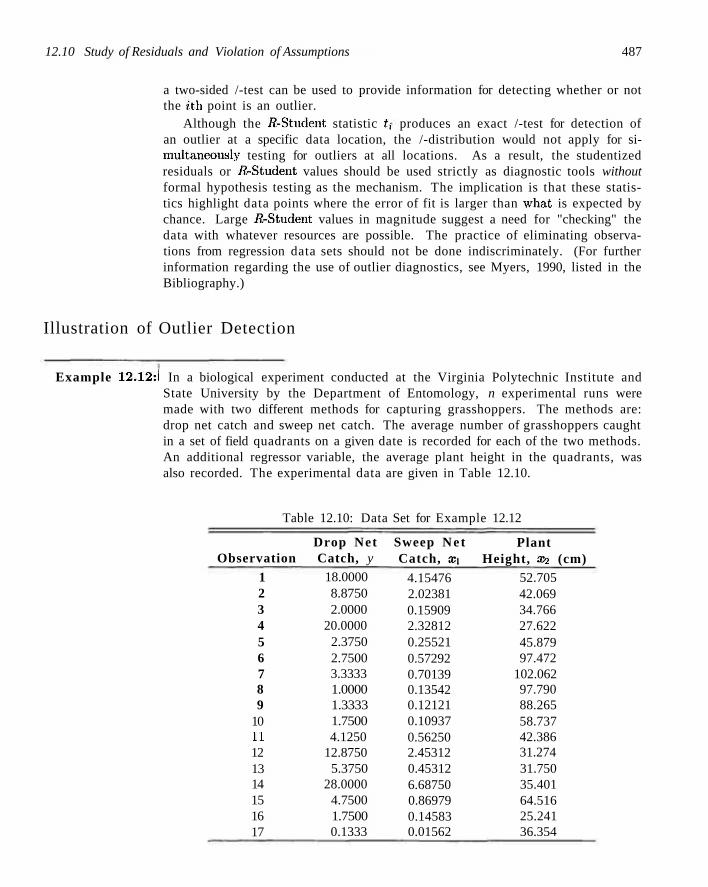
12.10 Study of Residuals and Violation of Assumptions 487
a two-sided /-test can be used to provide information for detecting whether or not the tth point is an outlier.
Although the /2-Student statistic /, produces an exact /-test for detection of an outlier at a specific data location, the /-distribution would not apply for simultaneously testing for outliers at all locations. As a result, the studentized residuals or /{-Student values should be used strictly as diagnostic tools without formal hypothesis testing as the mechanism. The implication is that these statistics highlight data points where the error of fit is larger than wdiat is expected by chance. Large /{-Student values in magnitude suggest a need for "checking" the data with whatever resources are possible. The practice of eliminating observations from regression data sets should not be done indiscriminately. (For further information regarding the use of outlier diagnostics, see Myers, 1990, listed in the Bibliography.)
Illustration of Outlier Detection
Example 12.12:1 In a biological experiment conducted at the Virginia Polytechnic Institute and State University by the Department of Entomology, n experimental runs were made with two different methods for capturing grasshoppers. The methods are: drop net catch and sweep net catch. The average number of grasshoppers caught in a set of field quadrants on a given date is recorded for each of the two methods. An additional regressor variable, the average plant height in the quadrants, was also recorded. The experimental data are given in Table 12.10.
Table 12.10: Data Set for Example 12.12
Observation 1 2 3 4 5 6 7 8 9
10 11 12 13 14 15 16 17
Drop Net Catch, y
18.0000 8.8750 2.0000
20.0000 2.3750 2.7500 3.3333 1.0000 1.3333 1.7500 4.1250
12.8750 5.3750
28.0000 4.7500 1.7500 0.1333
Sweep Net Catch, xi
4.15476 2.02381 0.15909 2.32812 0.25521 0.57292 0.70139 0.13542 0.12121 0.10937 0.56250 2.45312 0.45312 6.68750 0.86979 0.14583 0.01562
Plant Height, £2 (cm)
52.705 42.069 34.766 27.622 45.879 97.472
102.062 97.790 88.265 58.737 42.386 31.274 31.750 35.401 64.516 25.241 36.354

488 Chapter 12 Multiple Linear Regression and Certain Nonlinear Regression Models
The goal is to be able to estimate grasshopper catch by using only the sweep net method, which is less costly. There was some concern about the validity of the fourth data point. The observed catch that was reported using the net drop method seemed unusually high given the other conditions and, indeed, it was felt that the figure might be erroneous. Fit a model of the type
Pi =0O+0lXx + f%X2
to the 17 data points and study the residuals to determine if data point 4 is an outlier.
Solution: A computer package generated the fitted regression model
y = 3.6870 + 4.1050.fi - 0.0367£2
along with the statistics R2 = 0.9244 and s2 = 5.580. The residuals and other diagnostic information were also generated and recorded in Table 12.11.
Table 12.11: Residual Information for the Data Set of Example 12.12
Obs.
1 2 3 4 5 6 7 8 9
10 11 12 13 14 15 16 17
Vi
18.000 8.875 2.000
20.000 2.375 2.750 3.333 1.000 1.333 1.750 4.125
12.875 5.375
28.000 4.750 1.750 0.133
Vi 18.809 10.452 3.065
12.231 3.052 2.464 2.823 0.656 0.947 1.982 4.442
12.610 4.383
29.841 4.891 3.360 2.418
Vi - Vi -0.809 -1.577 -1.065
7.769 -0.677
0.286 0.510 0.344 0.386
-0.232 -0.317
0.265 0.992
-1.841 -0.141 -1.610 -2.285
hu
0.2291 0.0766 0.1364 0.1256 0.0931 0.2276 0.2669 0.2318 0.1691 0.0852 0.0884 0.1152 0.1339 0.6233 0.0699 0.1891 0.1386
Sy/1 — hu
2.074 2.270 2.195 2.209 2.250 2.076 2.023 2.071 2.153 2.260 2.255 2.222 2.199 1.450 2.278 2.127 2.193
n -0.390 -0.695 -0.485
3.517 -0.301
0.138 0.252 0.166 0.179
-0.103 -0.140
0.119 0.451
-1.270 -0.062 -0.757 -1.042
U
-0.3780 -0.6812 -0.4715
9.9315 -0.2909
0.1329 0.2437 0.1601 0.1729
-0.0989 -0.1353
0.1149 0.4382
-1.3005 -0.0598 -0.7447 -1.0454
As expected, the residual at the fourth location appears to be unusually high, namely, 7.769. The vital issue here is whether or not this residual is larger than one would expect by chance. The residual standard error for point 4 is 2.209. The R-Student value t4 is found to be 9.9315. Viewing this as a value of a random variable having a /-distribution with 13 degrees of freedom, one would certainly conclude that the residual of the fourth observation is estimating something greater than 0 and that the suspected measurement error is supported by the study of residuals. Notice that no other residual results in an /{-Student value that produces any cause for alarm. J

12.10 Study of Residuals and Violation of Assumptions 489
Plot t ing Residuals
In Chapter 11 wc discuss, in some detail, the usefulness of plotting residuals in regression analysis. Violation of model assumptions can often be detected through these plots. In multiple regression normal probability plotting of residuals or plots of residuals against y may be useful. However, it is often preferable to plot studentized residuals.
Keep in mind that the preference of the studentized residuals over ordinary residuals for plotting purposes stems from the fact that since the variance of the ith residual depends on the ith HAT diagonal, variances of residuals will differ if there is a dispersion in the HAT diagonals. Thus the appearance of a plot of residuals may depict heterogeneity because the residuals themselves do not behave, in general, in an ideal way. The purpose of using studentized residuals is to provide a standardization. Clearly, if a were known, then under ideal conditions (i.e., a correct model and homogeneous variance), we have
E [oy/T^hTi)
= 0, and Var ay/\ — hi
= 1.
So the studentized residuals produce a set of statistics that behave in a standard way under ideal conditions. Figure 12.5 shows a plot of the /{-Student values for the grasshopper data of Example 12.12. Note how the value for observation 4 stands out from the rest. The /{-Student plot was generated by SAS software. The plot shows the residual against the y-values.
T 10 15 20
Predicted Value of Y
T 25 30
Figure 12.5: /{-Student values plotted against predicted values for grasshopper data of Example 12.12.

490 Chapter 12 Multiple Linear Regress ion. and Certain Nonlinear Regression Models
Normality Checking
The reader should recall the importance of normality checking through the use of normal probability plotting as discussed in Chapter 11. The: same recommendation holds for the case of multiple linear regression. Normal probability plots can be generated using standard regression software. Again, however, they can be more effective when one does not use ordinary residuals but, rather, studentized residuals or /{-Student values.
12.11 Cross Validation, Cp, and Other Criteria for Model Selection
For many regression problems the experimenter must choose between various alternative models or model forms that are developed from the same data set. Quite often, in fact, the model that best predicts or estimates mean response is required. The experimenter should fake into account the relative sizes of the .s,2-values for the candidate models and certainly the general nature of the confidence intervals on the mean response. One must also consider how well the model predicts response values that were not used in building the candidate models. The models should be subjected to cross validation. What, is required, then, are cross-validation errors rather than fitting errors. Such errors in prediction are the PRESS residuals
Si = Vi ~§i,-i, i = 1,2,
where ?/,;._,• is the prediction of the ith data point by a model that did not. make use of the ith point in the calculation of the coefficients. These PRESS residuals are calculated from the formula
fc-i-Ar-. i=l,2,...,n, 1 - li.,t
(The derivation can be found in the regression textbook by Myers, 1990).
Use of the PRESS Statistic
The motivation for PRESS and the utility of PRESS residuals is very simple to understand. The purpose of extracting or setting aside data, points one at a time is to allow the use; of separate methodologies for fitting and assessment of a specific model. For assessment of a model the "—f indicates that the PRESS residual gives a prediction error where the observation being predicted is independent of the model, fit.
Criteria that make use of the PRESS residuals are given by
Y,\5i\ and PRESS = J^«f. 2 = 1
The term PRESS is an acronym for the prediction sum of squares. We suggest that both of these criteria be used. It is possible for PRESS to be dominated by one

12.11 Cross Validation, Cp, and Other Criteria for Model Selection 491
n or only a few large PRESS residuals. Clearly, the criteria YI \°i\ }S l e s s sensitive
i = l to a small number of large values.
In addition to the PRESS statistic itself, the analyst can simply compute an "R2-hke" statistic reflecting prediction performance. The statistic is often called R2
d and is given as follows:
R? of Prediction Given a fitted model with a specific value for PRESS, R2red is given by
PRESS R2 - 1 •"•pred ±
Zivi-v)2
i=X
Note that. /{2 (1 is merely the ordinary R2 statistic with SSE replaced by the
PRESS statistic. In the following example a "case-study" illustration is provided in which many-
candidate models are fit to a set of data and the best model is chosen. The sequential procedures described in Section 12.9 are not used. Rather, the role of the PRESS residuals and other statistical values in selecting the best regression equation is illustrated.
Example 12.13:1 Case S tudy Leg strength is a necessary ingredient of a successful punter in American football. One measure of the quality of a good punt is the "hang time." This is the time that the ball hangs in the air before being caught by the punt returner. To determine what leg strength factors influence hang time and to develop an empirical model for predicting this response, a study on The Relationship Between Selected Physical Performance Variables and Football Punting Ability was conducted by the Department of Health, Physical Education, and Recreation at the Virginia Polytechnic Institute and State University. Thirteen punters were chosen for the experiment and each punted a football 10 times. The average hang time, along with the strength measures used in the analysis, were recorded in Table 12.12.
Each regressor variable is defined as follows:
1. RLS, right leg strength (pounds)
2. LLS, left leg strength (pounds)
3. RHF, right hamstring muscle flexibility (degrees)
4. LHF, left hamstring muscle flexibility (degrees)
5. Power, Overall leg strength (foot-pounds)
Determine the most appropriate model for predicting hang time. Solution: In the search for the "best" of the candidate models for predicting hang time, the
information in Table 12.13 was obtained from a regression computer package. The models are ranked in ascending order of the values of the PRESS statistic. This display provides enough information on all possible models to enable the user to eliminate from consideration all but a few models. The model containing x2 and £5 (LL5and Power), denoted by £2£s, appears to be superior for predicting punter

492 Chapter 12 Multiple Linear Regression and Certain Nonlinear Regression Models
Table 12.12: Data for Example 12.13
Punter
1 2 3 4 5 6 7 8 9
10 11 12 13
Hang Time, V (sec)
4.75 4.07 4.04 4.18 4.35 4.16 4.43 3.20 3.02 3.64 3.68 3.60 3.85
RLS, Xx 170 140 180 160 170 150 170 110 120 130 120 140 160
LLS, X2
170 130 170 160 150 150 180 110 110 120 140 130 150
RHF, x3
106 92 93
103 104 101 108 86 90 85 89 92 95
LHF, £4
106 93 78 93 93 87
106 92 86 80 83 94 95
Power, £5
240.57 195.49 152.99 197.09 266.56 260.56 219.25 132.68 130.24 205.88 153.92 154.64 240.57
hang time. Also note that all models with low PRESS, low .s2, low Y2 \^i\, and t= i
high /{2-values contain these two variables. In order to gain some insight from the residuals of the fitted regression
Pi =bo + b2x2i +b5x5i,
the residuals and PRESS residuals were generated. The actual prediction model (see Exercise 12.47 on page 496) is given by
y = 1.10765 + 0.01370.X-2 + 0.00429£5.
Residuals, hat diagonal values, and PRESS values are listed in Table 12.14. Note the relatively good fit of the two-variable regression model to the data.
The PRESS residuals reflect the capability of the regression equation to predict hang time if independent predictions were to be made. For example, for punter number 4, the hang time of 4.180 would encounter a prediction error of 0.039 if the model constructed by using the remaining 12 punters were used. For this model, the average prediction error or cross-validation error is
1=1
0.1489 second,
which is small compared to the average hang time for the 13 punters. J We indicate in Section 12.9 that the use of all possible subset regressions is often
advisable when searching for the best model. Most commercial statistics software packages contain all possible regressions routine. These algorithms compute various criteria for all subsets of model terms. Obviously, criteria such as R2, s2, and PRESS are reasonable for choosing among candidate subsets. Another very popular and useful statistic, particularly for areas in the physical sciences and engineering, is the Cp statistic, described below.

12.11 Cross Validation, C,,, and Other Criteria for Model Selection 493
Table 12.13: Comparing Different Regression Models
Model £1*1 PRESS R2
The Cv
X2X5
£l£'2£5
X2X4X$
x2x3x5
XiX2X.lX5
£ l £ 3 £ 3 £ 5
£2 £3 £4^5
£l £3.1:5
£l £.l£5
Xixr, x2x3
XiX3
XxX2X3X4Xs
£2
£3*5
£l£2
x3
£l£3£.-l
£2«3X4
X2X,i
X\X2X3
X3X<\
X1X4
X\
£ 1£ 3£4£ 3
£l£2£4
£3£.l£5
£l£2£3£4
£5
£.l£5
£.1
Statistic
0.036907 0.041001 0.037708 0.039636 0.042265 0.044578 0.042421 0.053664 0.056279 0.059621 0.056153 0.059400 0.048302 0.066894 0.065678 0.068402 0.074518 0.065414 0.062082 0.063744 0.059670 0.080605 0.069965 0.080208 0.059169 0.064143 0.072505 0.066088 0.111779 0.105648 0.186708
1.93583 2.06489 2.18797 2.09553 2.42194 2.26283 2.55789 2.65276 2.75390 2.99434 2.95310 3.01436 2.87302 3.22319 3.09474 3.09047 3.06754 3.36304 3.32392 3.59101 3.41287 3.28004 3.64415 3.31562 3.37362 3.89402 3.49695 3.95854 4.17839 4.12729 4.88870
0.54683 0.58998 0.59915 0.66182 0.67840 0.70958 0.86236 0.87325 0.89551 0.97483 0.98815 0.99697 1.00920 1.04564 1.05708 1.09726 1.13555 1.15043 1.17491 1.18531 1.26558 1.28314 1.30194 1.30275 1.36867 1.39834 1.42036 1.52344 1.72511 1.87734 2.82207
0.871300 0.871321 0.881658 0.875606 0.882093 0.875642 0.881658 0.831580 0.823375 0.792094 0.804187 0.792864 0.882096 0.743404 0.770971 0.761474 0.714161 0.794705 0.805163 0.777716 0.812730 0.718921 0.756023 0.692334 0.834936 0.798692 0.772450 0.815633 0.571234 0.631593 0.283819
Quite often the choice of the most appropriate model involves many considerations. Obviously, the number of model terms is important; the matter of parsimony is a consideration that cannot be ignored. On the other hand, the analyst cannot be pleased with a model that is too simple, to the point where there is serious underspecification. A single statistic that represents a nice compromise in this regard is the Cp statistic. (See the Mallows reference in the Bibliography.)
The Cv statistic appeals nicely to common sense and is developed from considerations of the proper compromise between excessive bias incurred when one underfits (chooses too few model terms) and excessive prediction variance produced when one overfits (has redundancies in the model). The Cp statistic is a

494 Chapter 12 Multiple Linear Regression and Certain Nonlinear Regression Models
Table 12.14: PRESS Residuals
Punter 1 2 3 4 5 6 7 8 9
10 11 12 13
Vi 4.750 4.070 4.040 4.180 4.350 4.160 4.430 3.200 3.020 3.640 3.680 3.600 3.850
Vi 4.470 3.728 4.094 4.146 4.307 4.281 4.515 3.184 3.174 3.636 3.687 3.553 4.196
e* =Vi ~ Vi 0.280 0.342
-0.054 0.034 0.043
-0.121 -0.085
0.016 -0.154
0.004 -0.007
0.047 -0.346
hu 0.198 0.118 0.444 0.132 0.286 0.250 0.298 0.294 0.301 0.231 0.152 0.142 0.154
Si
0.349 0.388
-0.097 0.039 0.060
-0.161 -0.121
0.023 -0.220
0.005 -0.008
0.055 -0.409
simple function of the total number of parameters in the candidate model and the mean square error s2.
We will not present the entire development of the Cp statistic. (For details the reader is referred to the textbook by Myers in the Bibliography.) The Cp for a particular subset model is an estimate of the following:
i n 1 n
r(p) = ^ £ V a r ^ ) + 3 E ( B i a s &¥• i= l t=l
It turns out that under the standard least squares assumptions indicated earlier in this chapter, and assuming that the "true" model is the model containing all candidate variables.
1 -— Y j Var(yi) = p (number of parameters in the candidate model)
t = i
(see Review Exercise 12.61) and an unbiased estimate of
- l ^ B i a s y , ) 2 is given by ±fffi* yt? = ^JZSf^A. i=l i=l
In the above, s2 is the mean square error for the candidate model, and CJ2 is the population error variance. Thus if we assume that some estimate a2 is available for er2, Cp is given by
Cp Statistic (s2 - a2)(n - p) Cp = p+ ^2 ,
where p is the number of model parameters, s2 is the mean square error for the candidate model, and CT2 is an estimate of a2.

12.11 Cross Validation, Cp, and Other Criteria for Model Selection 495
Table 12.15: Data for Example 12.14
District 1 2 3 4 5 6 7 8 9
10 11 12 13 14 15
Promotional Accounts, £i
5.5 2.5 8.0 3.0 3.0 2.9 8.0 9.0 4.0 6.5 5.5 5.0 6.0 5.0 3.5
Active Accounts, x2
31 55 67 50 38 71 30 56 42 73 60 44 50 39 55
Competing Brands, x3
10 8
12 7 8
12 12 5 8 5
11 12 6
10 10
Potential, X\
8 6 9
16 15 17 8
10 4
16 7
12 6 4 4
Sales, y (Thousands)
$ 79.3 200.1 163.2 200.1 146.0 177.7 30.9
291.9 160.0 339.4 159.6 86.3
237.5 107.2 155.0
Obviously, the scientist should adopt models with small values of Cp. The reader should note that, unlike the PRESS statistic, Cp is scale-free. In addition, one can gain some insight concerning adequacy of a candidate model by observing its value of Cp. For example, Cp > p indicates a model that is biased due to being an underfitted model, whereas Cp ~ p indicates a reasonable model.
There is often confusion concerning wdiere d2 comes from in the formula for Cp. Obviously, the scientist or engineer does not have access to the population quantity <j2. In applications where replicated runs are available, say in an experimental design situation, a model-independent estimate of cr2 is available (see Chapters 11 and 15). However, most software packages use cr2 as the mean square error from the most complete model. Obviously, if this is not a good estimate, the bias portion of the Cp statistic can be negative. Thus Cp can be less than p.
Example 12.14:1 Consider the data set in Table 12.15, in which a maker of asphalt shingles is interested in the relationship between sales for a particular year and factors that influence sales. (The data were taken from Neter, Wassermann, and Kutner; see the Bibliography.)
Of the possible subset models, three are of particular interest. These three are £2£3, £i£2£3, and £i£2£3£4- The following represents pertinent information for comparing the three models. We include the PRESS statistics for the three models to supplement the decision making.
Model R2 R? PRESS
£ 2 £ 3
£ l £ 2 * 3 XXX2X3X4
0.9940 0.9970 0.9971
0.9913 0.9928 0.9917
44.5552 24.7956 26.2073
782.1896 643.3578 741.7557
11.4013 3.4075 5.0

496 Chapter 12 Multiple Linear Regression and Certain Nonlinear Regression. Models
Dependent V a r i a b l e : s a l e s Number in
Model
3 4 2 3 3 2 2 1 3 2 2 1 2 1 1
C(p)
3.4075 5.0000
11.4013
13.3770
1053.643
1082.670
1215.316
1228.460
1653.770
1668.699
1685.024
1693.971
3014.641
3088.650 3364.884
R-Square
0.9970
0.9971
0.9940
0.9940
0.6896
0.6805
0.6417
0.6373
0.5140
0.5090
0.5042
0.5010
0.1151
0.0928 0.0120
Adjusted
R-Square
0.9961 0.9959
0.9930
0.9924
0.6049
0.6273
0.5820
0.6094
0.3814
0.4272
0.4216
0.4626 -.0324
0.0231
-.0640
MSE
24.79560
26.20728
44.55518
48.54787
2526.96144
2384.14286
2673.83349
2498.68333
3956.75275
3663.99357
3699.64814
3437.12846
6603.45109
6248.72283
6805.59568
Variables i
xl xl x2 x2 xl x3 xl x3 xl xl x2 x2 xl x4 xl
x2 x2 x3 x3 x3 x4 x3
x2 x2 x4
x4
x3 x3 x4
x4 x4
x4
Figure 12.6: SAS printout of all possible subsets on sales da ta for Example 12.14.
It seems clear from the information in the table that the model xi,x2,x3 is preferable to the other two. Notice that , for the full model, Cp = 5.0. This occurs since the bias portion is zero, and a2 = 26.2073 is the mean square error from the full model. J
Figure 12.6 is a 5.45 PROC REG annotated printout showing information for all possible regressions. Here we are able to show comparisons of other models with (xi,x2,x3). Note that (xi,X2,Xs) appears to be quite good when compared to all models.
As a final check on the model (xi>X2,X3), Figure 12.7 shows a normal probability plot of the residuals for this model.
Exercises
12.47 Consider the "hang time" punting data given in Example 12.13, using only the variables x2 and x3.
(a) Verify the regression equation shown on page 492. (b) Predict punter hang time for a punter with LLS =
180 pounds and Power = 260 foot-pounds. (c) Construct a 95% confidence interval for the mean
hang time of a punter with LLS = 180 pounds and Power = 260 foot-pounds.
12.48 For the data of Exercise 12.11 on page 454, use the techniques of
(a) forward selection with a 0.05 level of significance to choose a linear regression model;
(b) backward eliniinalion with a 0.05 level of significance to choose a linear regression model;
(c) stepwise regression with a 0.05 level of significance to choose a linear regression model.
12.49 Use the techniques of backward elimination with a = 0.05 to choose a prediction equation for the data of Table 12.8.

Exercises 497
- 1 0 1
Theoretical Quantiles
Figure 12.7: Normal probability plot of residuals using the model £i£2£3 for Example 12.14.
12.50 For the punter data in Example 12.13, an additional response, "punting distance," was also recorded. The following are average distance values for each of the 13 punters:
Punter
1 2 3 4 5 6 7 8 9 10 11 12 13
Distance, y (ft)
162.50 144.00 147.50 163.50 192.00 171.75 162.00 104.93 105.67 117.59 140.25 150.17 165.16
(a) Using the distance data rather than the hang times, estimate a multiple linear regression model of the type
PY\xi,X2,X3,x4,X5
= 00 + j3lXl + 32^2 + 03X3 + #ia\] + 05X3
for predicting punting distance. (b) Use stepwise regression with a significance level of
0.10 to select a combination of variables. 13
(c) Generate values for s2, R2, PRESS, and YI l&l f o r
the entire set of 31 models. Use this information to determine the best combination of variables for predicting punting distance.
(d) For the final model you choose plot the standardized residuals against. Y and do a normal probability plot of the ordinary residuals. Comment.
12.51 The following is a set of data for y, the amount of money (thousands of dollars) contributed to the alumni association at Virginia Tech by the Class of 1960, and x, the number of years following graduation:
y 812.52 822.50 1211.50 1348.00 1301.00 2567.50 2526.50
X
1 2 3 4 8 9 10
y 2755.00 4390.50 5581.50 5548.00 6086.00 5764.00 8903.00
X
11 12 13 14 15 16 17
(a) Fit a regression model of the type
PY\x = 00 +0lX.
(b) Fit a quadratic model of the type
HY\x =0o + 0\x + 3nx .
(c) Determine which of the models in (a) or (b) is preferable. Use s2, R2, and the PRESS residuals to support your decision.

498 Chapter 12 Multiple Linear Regression and Certain Nonlinear Regression Models
12.52 For the model of Exercise 12.50(a), test the hypothesis
Ho: 34 = 0,
Hi: 3,i # 0.
Use a P-value in your conclusion.
12.53 For the quadratic model of Exercise 12.51(b), give estimates of the variances and covariances of the estimates of 0\ and 0i i.
12.54 In an effort to model executive compensation for the year 1979, 33 firms were selected, and data were gathered on compensation, sales, profits, and employment. Consider the model
yt =0o + 0i lnrnii + 02 \nx2i
+ 03\nx3i + ei, i = 1,2 33.
(a) Fit the regression with the model above. (b) Is a model with a subset of the variables preferable
to the full model?
12.55 Rayon whiteness is an important factor for scientists dealing in fabric quality. Whiteness is affected by pulp quality and other processing variables. Some of the variables include acid bath temperature, °C (xi); cascade acid concentration, % (a^); water temperature, °C (x3); sulfide concentration, % (aii); amount of chlorine bleach, lb/min (xs)\ blanket finish temperature, °C (.%). A set of data taken on rayon specimens is given here. The response, y, is the measure of whiteness.
(a) Use the criteria MSE, Cp, and PRESS to give the best model from among all subset models.
(b) Do a normal probability plot of residuals for the "best" model. Comment.
Firm 1 2 3 4 5 6 7 8 9
10 11 12 13 14 15 16 17 18 19 20 21 22 23 24 25 26 27 28 29 30 31 32 33
Compensation, y Sales, xi
(thousands) (millions) $450 387 368 277 676 454 507 496 487 383 311 271 524 498 343 354 324 225 254 208 518 406 332 340 698 306 613 302 540 293 528 456 417
$4,600.6 9,255.4 1,526.2 1,683.2 2. 752.8 2.205.8 2.384.6 2.746.0 1,434.0
470.6 1,508.0
464.4 9,329.3 2,377.5 1,174.3
409.3 724.7 578.9 966.8 591.0
4,933.1 7,613.2 3,457.4
545.3 22,862.8
2,361.0 2,614.1 1,013.2 4,560.3
855.7 4,211.6 5, 440.4 1.229.9
Profits, x2 (millions)
$128.1 783.9 136.0 179.0 231.5 329.5 381.8 237.9 222.3
63.7 149.5 30.0
577.3 250.7
82.6 61.5 90.8 63.3 42.8 48.5
310.6 491.6 228.0
54.6 3011.3
203.0 201.0 121.3 194.6 63.4
352.1 655.2
97.5
Employment , x3
48. 000 55.900 13.783 27.765 34.000 26.500 30.800 41.000 25.900 8.600
21.075 6,874
39,000 34,300 19.405 3.586 3.905 4.139 6,255
10,605 65, 392 89,400 55, 200
7,800 337.119
52, 000 50, 500 18, 625 97,937 12,300 71,800 87, 700 14,600
y X\ X2 £ l X.l X5 X6
88.7 89.3 75.5 92.1 83.4 44.8 50.9 78.0 86.8 47.3 53.7 92.0 87.9 90.3 94.2 89.5
43 42 47 46 52 50 43 49 51 51 48 46 43 45 53 47
0.211 0.604 0.450 0.641 0.370 0.526 0.486 0.504 0.609 0.702 0.397 0.488 0.525 0.486 0.527 0.601
85 89 87 90 93 85 83 93 90 80 92 88 85 84 87 95
0.243 0.237 0.198 0.194 0.198 0.221 0.203 0.279 0.220 0.198 0.231 0.211 0.199 0.189 0.245 0.208
0.606 0.600 0.527 0.500 0.485 0.533 0.510 0.489 0.462 0.478 0.411 0.387 0.437 0.499 0.530 0.500
48 55 61 6a 54 60 57 49 64 63 61 88 63 58 65 67
12.56 A client from the Department of Mechanical Engineering approached the Consulting Center at Virginia Polytechnic Institute and State University for help in analyzing an experiment dealing with gas turbine engines. Voltage output of engines was measured at various combinations of blade speed and voltage measuring sensor extension. The data are as follows:
y (volts)
1.95 2.50 2.93 1.69 1.23 3.13 1.55 1.94 2.18 2.70 1.32 1.60 1.89
Speed , £i (in. / sec )
6336 7099 8026 6230 5369 8343 6522 7310 7974 8501 6646 7384 8000
Extension, X2 ( in . )
0.000 0.000 0.000 0.000 0.000 0.000 0.006 0.006 0.006 0.006 0.012 0.012 0.012

12.12 Special Nonlinear Models for Nonidenl Conditions 499
(a) Fit a regression model using all independent variables.
(b) Use stepwise regression with input significance level 0.25 and removal significance level 0.05. Give your final model.
(c) Use all possible regression models and compute R.~, Cv, s~, adjusted R~ for all models.
(d) Give final model.
(e) For your model in part (d), plot studentized residuals (or fl-Student) and comment.
y (volts)
2.15 1.09 1.26 1.57 1.92
Speed, xi ( in . /sec)
8545 6755 7362 7934 8554
Ex tens ion , xj ( in . )
0.012 0.018 0.018 0.018 0.018
(a) Fit a multiple linear regression to the data, (h) Compute (-tests on coefficients. Give P-values. (c) Comment on the quality of the fined mode:!.
12.57 The pull strength of a wire bond is an inipor- 1 2 5 8 F()|. B x ( T c i s ( , l 2 .57, test H0: 0i = f% = 0. Give taut, characteristic. rIhe table below gives Information p.values and comment on pull strength y, die height xi, post height x2, loop height Xi, wire length a*, bond width on the die xr,, 12.59 In Exercise- 12.28, page 464, we have the fol-anel bond width on the post x6. [Data from Myers and lowing data concerning wear of a bearing: .Montgomery (2002).]
y (wear) £j (oil viscosity) x2 ( load) 1. Ei x- ^ ^1 S 5 L _ 193 1.0 851
230 15.5 816 172 22.0 1058 91 43.0 1201
113 33.0 1357 125 40.0 1115
(a) The following model may be considered to describe this data:
yi = 00 + 0\Xl, + ,32X21 + 0\2XUX2i + «,,
8.0 8.3 8.5 8.8 9.0 9.3 9.3 9.5 9.8
10.0 10.3 10.5 10.8 11.0 11.:', 11.5 11.8 12.3 12.5
5.2 5.2 5.8 6.4 5.8 5.2 5.6 6.0 5.2 5.8 0.4 6.0 6.2 6.2 6.2 5.6 6.0 5.8 5.6
19.6 19.8 19.6 19.4 18.6 18.8 20.4 19.0 20.8 19.9 18.0 20.6 20.2 20.2 19.2 17.0 19.8 18.8 18.6
29.6 32.4 31.0 32.4 28.6 30.6 32.4 32.6 32.2 31.8 32.6 33.4 31.8 32.4 31.4 33.2 35.4 34.0 34.2
94.9 89.7 96.2 95.6 86.5 84.5 88.8 85.7 93.6 86.0 87.1 93.1 83.4 94.5 83.4 85.2 84.1 80.9 83.0
2.1 2.1 2.0 2.2 2.0 2.1 2.2 2.1 2.3 2.1 2.0 2.1 2.2 2.1 1.9 2.1 2.0 2.1 1.9
2.3 1.8 2.0 2.1 1.8 2.1 1.9 1.9 2.1 1.8 1.(1 2.1 2.1 1.9 1.8 2.1 1.8 1.8 2.0
for i = 1 ,2 , . . . ,6 . The %\X2 is an "interaction"' term. Fit this model and estimate the parameters.
(b) Use the models (x\), (£1,12), (x2). (xi ,£2,£i£a) and compute PRESS, Cp, and s" to determine the 'best'' model.
12.12 Special Nonlinear Models for Nonideal Conditions
In much of the preceding material in this chapter and in Chapter 11 wc have benefited substantially from the assumption tha t the model errors, the ei, are normal with mean zero and constant variance o . However, there are many real-life situations in which the response is clearly nonnormal. For example, a wealth of applications exist where the r e s p o n s e is b i n a r y (0 or 1) and hence Bernoulli in nature . In the1 social sciences the problem may be to develop a model to predict whether or not an individual is a good credit risk or not (0 or 1) as a function of certain socioeconomic regressors such as income, ago, gender and level of education. In a biomedical drug trial the response is often whether or not the patient responds positively to a drug while regressors may include drug dosage as well as biological factors such us age, weight, and blood pressure. Again the response is binary

500 Chapter 12 Multiple Linear Regression and Certain Nonlinear Regression Models
in nature. Applications are also abundant in manufacturing areas where certain controllable factors influence whether a manufactured item is defective or not.
A second type of nonnormal application on which we will touch briefly has to do with count data. Here the assumption of a Poisson response is often convenient. In biomedical applications the number of cancer cell colonies may be the response which is modeled against drug dosages. In the textile industry the number of imperfections per yard of cloth may be a reasonable response which is modeled against certain process variables.
Nonhomogeneous Variance
The reader should note the comparison of the ideal (i.e., the normal response) situation with that of the Bernoulli (or binomial) or the Poisson response. We have become accustomed to the fact that the normal case is very special in that the variance is independent of the mean. Clearly this is not the case for either Bernoulli or Poisson responses. For example, if the response is 0 or 1, suggesting a Bernoulli response, then the model is of the form
p = f(x.0),
where p is the probability of a success (say response = 1). The parameter p plays the role of py\x in the normal case. However, the Bernoulli variance is »(1 - p), which, of course, is also a function of the regressor x. As a result, the variance is not constant. This rules out the use of standard least squares that we have utilized in our linear regression work up to this point. The same is true for the Poisson case since the model is of the form
X = fix,0),
with Var(y) = uv = A. which varies with x.
Binary Response (Logistic Regression)
The most popular approach to modeling binary responses is a technique entitled logistic regression. It is used extensively in the biological sciences, biomedical research, and engineering. Indeed, even in the social sciences binary responses are found to be plentiful. The basic distribution for the response is either Bernoulli or binomial. The former is found in observational studies where there are no repeated runs at each regressor level while the latter will be the case when an experiment is designed. For example, in a clinical trial in which a new drug is being evaluated the goal might be to determine the dose of the drug that provides efficacy. So certain doses will be employed in the experiment and more than one subject will be used for each dose. This case is called the grouped case.
W h a t Is the Model for Logistic Regression?
In the case of binary responses the mean response is a probability. In the preceding clinical trial illustration, we might say that we wish to estimate the probability that

12.12 Special Nonlinear Models for Nonideal Conditions 501
the patient responds properly to the drug (P(success)). Thus the model is written in terms of a probability. Given regressors x, the logistic function is given by
P = 1
1 + e-* '" '
The portion x'3 is called the linear predictor and in the case of a single regressor x it might be written x'0 = 0O + 0ix. Of course, we do not rule out involving multiple regressors and polynomial terms in the so-called linear predictor. In the grouped case the model involves modeling the mean of a binomial rather than a Bernoulli and thus we have the mean given by
np = n
1+e -x'3'
Characteristics of Logistic Function
A plot of the logistic function reveals a great deal about its characteristics and why it is utilized for this type of problem. First, the function is nonlinear. In addition, the plot in Figure 12.8 reveals the S-shape with the function approaching p = 1.0 as an asymptote. In this case 0i > 0. Thus we would never experience an estimated probability exceeding 1.0.
Figure 12.8: The logistic function.
The regression coefficients in the linear predictor can be estimated by the method of maximum likelihood as described in Chapter 9. The solution to the likelihood equations involves an iterative methodology that will not be described here. However, we will present an example and discuss the computer printout and conclusions.
Example 12.15: The data set in Table 12.16 is an example of the use of logistic regression to analyze a single agent quantal bioassay of a toxicity experiment. The results show the effect of different doses of nicotine on the common fruit fly.
The purpose of the experiment was to use logistic regression to arrive at an appropriate model relating probability of "kill" to concentration. In addition, the

502 Chapter 12 Multiple Linear Regression and Certain Nonlinear Regression Models
Table 12.16: Data Set for Example 12.15
X
Concentration (g rams/100
0.10 0.15 0.20 0.30 0.50 0.70 0.95
cc)
iy Number of
Insects 47 53 55 52 46 54 52
y Number
Killed
8 14 24 32 38 50 50
Percent Killed
17.0 26.4 43.6 61.5 82.6 92.6 96.2
analyst sought the so-called effective dose (ED), that is, the concentration of nicotine that results in a certain probability. Of particular interest is the ED50, the concentration that produces a 0.5 probability of "insect kill."
This example is grouped and thus the model is given by
E(Yi) = mpi = 1 4. e-(%+&\Xi)'
Estimates of 0Q and 0\ and their standard errors are found by maximum likelihood. Tests on individual coefficients are found using x2-statistics rather than ^-statistics since there is no common variance a2. The x2-statistic is derived from / coeff \ 2
\ standard error/ Thus we have the following from a SMS PROC LOGIST printout.
00 01
df 1 1
Estimate -1.7361
6.2954
Analysis of Parameter Estimates Standard Error Chi-Squared
0.2420 51.4482 0.7422 71.9399
P-value
< 0.0001 < 0.0001
Both coefficients are significantly different from zero. Thus the fitted model used to predict the probability of "kill" is given by
1 P = 1 _|_ e-(-1.73(il+0.2954x) '
Est imate of Effective Dose
The estimate of ED50 is found very simply from the estimate 60 for 0Q and 61 for 0x. From the logistic function, we see that
\og(-^-\=0Q+0xx.
As a result for p = 0.5, an estimate of x is found from
60 + bxx = 0.

Review Exercises 503
Thus the ED50 is given by
x = - ( ~ j = 0.276 grams/100 cc.
Concept of Odds Ratio
Another form of inference tha t is conveniently accomplished using logistic regression is derived from the use of the odds rat io. The odds rat io is designed to
Definition 12.1:
determine how the o d d s of succes s = j ^ — increases as certain changes in regressor values occur. For example, in the case of Example 12.15 we may wish to know how the odds increases if one were to increase dosage by, say, 0.2 gram/lOOcc.
In to
logistic regression that of condition
an odds ratio is 1 in the regressort
b/(i-b/U-
the ratio of odds of , that is,
P)h p)W
success at condition 2
This allows the analyst to ascertain a sense of the utility of changing the regressor
by a certain number of units. Now since ( j ^ - ) = eth+f>\--r^ (-uen for o u r Example
12.15, the rat io reflecting the increase in odds of success when dosage of nicotine is increased by 0.2 grams/100 cc is given by
gO.26, _ e(0.2)(6.2954) _ 3 ^2.
The implication of an odds ratio of 3.522 is t ha t the odds of success is enhanced by a factor of 3.522 when the nicotine dose is increased by 0.2 g rams/100 cc.
Review Exercises
12.60 In the Department of Fisheries and Wildlife at Virginia Polytechnic Institute and State University, an experiment was conducted to study the effect of stream characteristics on fish biomass. The regressor variables are as follows: average depth (of 50 cells) (xi): area of in-stream cover (i.e., undercut banks, logs, boulders, etc.) (as); percent canopy cover (average of 12) (x3); area> 25 centimeters in depth (x4). The response is y, the fish biomass. The data are as follows:
Obs . y Xl X2 Xa X.l
1 2 3 4 5 6 7 8
100 388 755
1288 230
0 551 345
14.3 19.1 54.6 28.8 16.1 10.0 28.5 13.8
15.0 29.4 58.0 42.6 15.9 56.4 95.1 60.6
12.2 26.0 24.2 26.1 31.6 23.3 13.0 7.5
48.0 152.2 469.7 485.9
87.6 6.9
192.9 105.8
Obs. V Xi X2 Xi X l
9 0 10.7 35.2 40.3 0.0 10 348 25.9 52.0 40.3 116.6
(a) Fit a multiple linear repression including all four regression variables.
(b) Use Cp , R2, and s to determine the best subset of variables. Compute these statistics for all possible subsets.
(c) Compare the appropriateness of the models in parts (a) and (b) for predicting fish biomass.
12.61 Show that, in a multiple linear regression data set,
53 /j« = ?'•

504 Chapter 12 Multiple Linear Regression and Certain Nonlinear Regression Models
12.62 A small experiment is conducted to fit a multiple regression equation relating the yield y to temperature Xi, reaction time x2, and concentration of one of the reactants xs. Two levels of each variable were chosen and measurements corresponding to the coded independent variables were recorded as follows:
y X\ 3>2 X3
efficient response
7.6 5.5 9.2
10.3 11.6 11.1 10.2 14.0
- 1 1
- 1 - 1
1 1
- 1 1
- 1 - 1
1 - 1
1 - 1
1 1
- 1 - 1 - 1
1 - 1
1 1 1
(a) Using the coded variables, estimate the multiple linear regression equation
UY\x = 3a + 01-t'l + 02'-t2 + 53J3.
(b) Partition SSR, the regression sum of squares, into three single3-degree-of-freedom components attributable to x i , 2-2, and x3, respectively. Show an analysis-of-variance table, indicating significance tests on each variable. Comment of the results.
12.63 In a chemical engineering experiment dealing with heat transfer in a shallow fluidized bed, data are collected on the following four regressor variables: flu-idizing gas flow rate, lb/hr (xi); supernatant gas flow rate, lb/hr (X2); supernatant gas inlet nozzle opening, millimeters (as); supernatant gas inlet temperature, °F (x4). The responses measured are heat transfer efficiency (yi): thermal efficiency (1/2). The data are as follows:
Obs . 2/i 2/2 Xl X-2 X.l XA
1 2 3 4 5 6 7 8 9
10 11 12 13 14 15 16 17 18 19 20
41.852 155.329 99.628 49.409 72.958 107.702 97.239 105.856 99.348 111.907 100.008 175.380 117.800 217.409 41.725 151.139 220.630 131.666 80.537 152.966
38.75 51.87 53.79 53.84 49.17 47.61 64.19 52.73 51.00 47.37 43.18 71.23 49.30 50.87 54.44 47.93 42.91 66.60 64.94 43.18
69.69 113.46 113.54 118.75 119.72 168.38 169.85 169.85 170.89 171.31 171.43 171.59 171.63 171.93 173.92 221.44 222.74 228.90 231.19 236.84
170.83 230.06 228.19 117.73 117.69 173.46 169.85 170.86 173.92 173.34 171.43 263.49 171.63 170.91 71.73 217.39 221.73 114.40 113.52 167.77
45 25 65 65 25 45 45 45 80 25 45 45 45 10 45 65 25 25 65 45
219.74 181.22 179.06 281.30 282.20 216.14 223.88 222.80 218.84 218.12 219.20 168.62 217.58 219.92 296.60 189.14 186.08 285.80 286.34 221.72
l/i i =00 + 5 3 0jXji + ^ 0}jX2i J = l
+ 5 3 5 Z PiiXii*" + e«"> « = 1,2,.. . , 20.
n (a) Compute PRESS and YI \yt — yt,-i\ for the least
i—l squares regression fit to the model above,
(b) Fit a second-order model with x4 completely eliminated (i.e., deleting all terms involving £1). Compute the prediction criteria for the reduced model. Comment on the appropriateness of x4 for prediction of the heat transfer coefficient.
(c) Repeat parts (a) and (b) for thermal efficiency.
12.64 In exercise physiology, an objective measure of aerobic fitness is the oxygen consumption in volume per unit body weight per unit time. Thirty-one individuals were used in an experiment in order to be able to model oxygen consumption against: age in years (11); weight in kilograms (as); time to run l | miles (3:3); resting pulse rate (x4); pulse rate at the end of run (as); maximum pulse rate during run (2$).
ID y Xl x3 214 XQ xa
Consider the model for predicting the heat transfer co-
1 2 3 4 5 6 7 8 9 10 11 12 13 14 15 16 17 18 19 20 21 22 23 24 25 26 27 28
44.609 45.313 54.297 59.571 49.874 44.811 45.681 49.091 39.442 60.055 50.541 37.388 44.754 47.273 51.855 49.156 40.836 46.672 46.774 50.388 39.407 46.080 45.441 54.625 45.118 39.203 45.790 50.545
44 40 44 42 38 47 40 13 44 38 44 45 •15 47 54 49 51 51 48 49 57 54 52 50 51 54 51 57
89.47 75.07 85.84 68.15 89.02 77.45 75.98 81.19 81.42 81.87 73.03 87.66 66.45 79.15 83.12 81.42 69.63 77.91 91.63 73.37 73.37 79.38 76.32 70.87 67.25 91.63 73.71 59.08
11.37 10.07 8.65 8.17 9.22 11.63 11.95 10.85 13.08 8.63 10.13 14.03 11.12 10.60 10.33 8.95 10.95 10.00 10.25 10.08 12.63 11.17 9.63 8.92 11.08 12.88 10.47 9.93
62 62 45 40 55 58 70 64 63 48 45 56 51 47 50 44 57 48 48 76 58 62 48 48 48 44 59 49
178 182 185 185 156 168 166 172 178 180 176 176 176 180 162 170 174 176 170 186 168 168 186 192 176 176 162 164 166 170 180 185 168 162
172 168
162 164 168 168 174 176 156 165 164 166 146 155 172 172 168 172 186 188 148 155

Review Exercises 505
ID y Xl x2 X-s XA X$
29 48.673 30 47.920 31 47.467
49 48 52
76.32 61.24 82.78
9.40 11.50 10.50
xe 56 186 188 52 170 176 53 170 172
(a) Do a stepwise regression with input significance level 0.25. Quote the final model.
(b) Do all possible subsets using s2, Cp, R2, and JR^JJ. Make a decision and quote the final model.
12.67 An article in the Journal of Pharmaceutical Sciences (Vol. 80, 1991) presents data on the mole fraction solubility of a solute at a constant temperature. Also measured are the dispersion a;i, and dipolar and hydrogen bonding solubility parameters as, and 3:3. A portion of the data is shown in the table below. In the model, y is the negative logarithm of the mole fraction. Fit the model
12.65 Consider the data of Review Exercise 12.62. Suppose it is of interest to add some "interaction" terms. Namely, consider the model
Vi = 0o+ 0iXu + 32X2i + 03X3i + 0\2xiiX2i
+ 013'XliX3i + 023X2iX3i + 0l23XliX2iX3i + Ci-
(a) Do we still have orthogonality? Comment.
(b) With the fitted model in part (a), can you find prediction intervals and confidence intervals on the mean response? Why or why not?
(c) Consider a model with ,6"i23a:ia:2.T3 removed. To determine if interactions (as a whole) are needed, test
Ho'- 0\1 = A3 = #23 = 0.
Give P-value and conclusions.
12.66 A carbon dioxide (CO2) flooding technique is used to extract crude oil. The CO2 floods oil pockets and displaces the crude oil. In the experiment, flow tubes are dipped into sample oil podcets containing a known amount of oil. Using three different values of flow pressure and three different values of dipping angles the oil pockets are flooded with CO2, and the percentage of oil displaced recorded. Consider the model
2/t =0o + 0\Xu + 02x2i + 0nx2u
+ 022X2i + 0l2XuX2i + €,.
Fit the model above to the data, and suggest any model editing that may be needed.
Pressure lb / in 2 , xi
1000 1000 1000 1500 1500 1500 2000 2000 2000
Source: Wang, G. Flooding Process,"
Dipping Angle,
0 15 30 0
15 30 0
15 30
X2
C. "Microscopic
Oil Recovery,
%, v 60.58 72.72 79.99 66.83 80.78 89.78 69.18 80.31 91.99
: Investigations of ' Journal of Petroleum Technology,
Vi = 00 + 0\Xli + 02X2i + 33X3i + €i,
fori = 1,2, . . . , 20.
(a) Test H0: 0i = p\ = 03 = 0. (b) Plot studentized residuals against xi, x2, and X3
(three plots). Comment. (c) Consider two additional models that are competi
tors to the models above:
Model 2:
Model 3:
Add Xi, x2, x3
Add Xi,x2,x3,xix2,xiX3,X2X3.
With these three models use PRESS and Cv to arrive at the best among the three.
Obs. y Xl X2 x3
1 2 3 4 5 6 7 8 9
10 11 12 13 14 15 16 17 18 19 20
0.2220 0.3950 0.4220 0.4370 0.4280 0.4670 0.4440 0.3780 0.4940 0.4560 0.4520 0.1120 0.4320 0.1010 0.2320 0.3060 0.0923 0.1160 0.0764 0.4390
7.3 8.7 8.8 8.1 9.0 8.7 9.3 7.6
10.0 8.4 9.3 7.7 9.8 7.3 8.5 9.5 7.4 7.8 7.7
10.3
0.0 0.0 0.7 4.0 0.5 1.5 2.1 5.1 0.0 3.7 3.6 2.8 4.2 2.5 2.0 2.5 2.8 2.8 3.0 1.7
0.0 0.3 1.0 0.2 1.0 2.8 1.0 3.4 0.3 4.1 2.0 7.1 2.0 6.8 6.6 5.0 7.8 7.7 8.0 4.2
34, N0.8, Aug. 1982.
12.68 A study was conducted to determine whether lifestyle changes could replace medication in reducing blood pressure among hypertensives. The factors considered were a healthy diet with an exercise program, the typical dosage of medication for hypertension, and no intervention. The pretreatment body mass index (BMI) was also calculated because it is known to affect blood pressure. The response considered in this study

506 Chapter 12 Multiple Linear Regression and Certain Nonlinear Regression Models
Dependent
Source Model Error Corrected
Var iable
Var iab le : y A n a l y s i s
DF 5
11 Tota l 16
Root MSE Dependent Mean Coeff Var
Label I n t e r c e p t I n t e r c e p t x l x2 x3 x4
x5
of Variance Sum of
Squares 490177488
4535052 494712540
642 .08838 4978.48000
12.89728 Parameter
DF
Average D a i l y P a t i e n t Load 1 Monthly X-Ray Exposure 1 Monthly Occupied Bed Days 1 E l i g i b l e Popula t ion Area/100
i n the 1
Average Length of P a t i e n t s 1 Stay in Days
Mean Square
98035498 412277
R-Square Adj R-Sq
Est imates
F Value 237 .79
0 .9908 0 .9867
Parameter Standard Estimate Error t Value
1962.94816 1071.36170 1 .83 -15 .85167
0 .05593 1.58962
-4 .2 1 8 6 7
97 .65299 - 0 . 1 6 0 .02126 2 . 6 3 3 .09208 0 .51 7 .17656 - 0 . 5 9
-394 .31412 209 .63954 - 1 . 8 8
Pr > F <.0001
Pr > | t | 0 .0941 0 .8740 0 .0234 0 .6174 0 .5685
0 .0867
Figure 12.9: 5.45 output for Review Exercise 12.69; part I.
was change in blood pressure. The variable group has the following levels.
1 = Healthy diet and an exercise program
2 = Medication
3 = No intervention
C h a n g e i n B l o o d P r e s s u r e
- 3 2 - 2 1 - 2 6 - 1 6 - 1 1 - 1 9 - 2 3
- 5 - 6
5 - 1 1
14
G r o u p
1 1 1 1 2 2 2 2 3 3 3 3
BMI 27.3 22.1 26.1 27.8 19.2 26.1 28.6 23.0 28.1 25.3 26.7 22.3
(a) Fit an appropriate model using the data above. Doess it appear that exercise and diet could be effectively useid to lower blood pressure? Explain your answer from the results.
(b) Would exercise and diet be an effective alternative to medication?
(Hint. You may wish to form the model in more than one way to answer both of these questions.)
12.69 Case S tudy : Consider the data set for Exercise 12.12, page 454 (hospital data). The data set is repeated here.
(a) The SAS PR.OC REG outputs provided in Figures 12.9 and 12.10 supply a considerable amount of information. Goals are to do outlier detection and eventually determine which model terms are to be used in the final model.
(b) Comment, on what other analyses should be run. (c) Run appropriate analyses and write your conclu
sions concerning the final model.
Site xi X2 X3 X.\ 3 5 1 2 3 4 5 6 7 8 9
10 11 12 13 14 15 16 17
15.57 44.02 20.42 18.74 49.20 44.92 55.48 59.28 94.39
128.02 96.00
131.42 127.21 252.90 409.20 463.70 510.22
2463 2048 3940 6505 5723
11520 5779 5969 8461
20106 13313 10771 15543 36194 34703 39204 86533
472.92 1339.75 620.25 568.33
1497.60 1365.83 1687.00 1639.92 2872.33 3655.08 2912.00 3921.00 3865.67 7684.10
12446.33 14098.40 15524.00
18.0 9.5
12.8 36.7 35.7 24.0 43.3 46.7 78.7
180.5 60.9
103.7 126.8 157.7 169.4 331.4 371.6
4.45 6.92 4.28 3.90 5.50 4.60 5.62 5.25 6.18 6.15 5.88 4.88 5.50 7.00
10.75 7.05 6.35
566.52 696.82
1033.15 1003.62 1611.37 1613.27 1854.17 2160.55 2305.58 3503.93 3571.59 3741.40 4026.52
10343.81 11732.17 15414.94 18854.45

Review Exercises 507
Obs 1 2 3 4 5 6 7 8 9 10 11 12 13 14 15 16 17
Dependent Variable 566.5200 696.8200
1033 1604 1611 1613 1854 2161 2306 3504 3572 3741 4027 10344 11732 15415 18854
Predicted Value
775 740
0251 6702 1104 1240 1564 2151 1690 1736 2737 3682 3239 4353 4257 8768 12237 15038 19321
Obs Residual 1 -208 2 -43 3 -70 4 363 5 46 6 -538 7 164 8 424 9 -431 10 -177 11 332 12 -611 13 -230 14 15 -504 16 376 17 -466
5051 8502 7734 1244 9483 0017 4696 3145 4090 .9234 6011 9330 5684 1576 8574 5491 2470
Std Error Mean Predict
241 331 278 268 211 279 218 468 290 585 189 328 314 252 573 585 599
Std Error Residual
595.0 550.1 578.5 583.4 606.3 577.9 603.6 438.5 572.6 264.1 613.6 551.5 560.0 590.5 287.9 263.1 228.7
2323 1402 5116 1298 2372 .9293 .9976 9903 4749 2517 0989 8507 0481 2617 9168 7046 9780
95% CL 244.0765 11.8355 490.9234 650.3459
1099 1535 1208
703.9948 2098 2394 2823 3630 3566 8213 10974 13749 18000
Student Residual
•0.350 -0.0797 -0.122 0.622 0.0774 -0.931 0.272 0.968 -0.753 -0.674 0.542 -1.110 -0.412 2.669 -1.753 1.431 -2.039
Mean 1306 1470 1717 1831 2029 2767 2172 2768 3376 4970 3655 5077 4948 9323 13500 16328 20641
-2-1 0 1
1 *
* 1
1* * i * 1 1*
**|
95'/, CL Predict -734.6494 -849.4275 -436.5244 -291.0028 76.6816 609.5796 196.5345 -13.8306
1186 1770 1766 2766 2684 7249 10342 13126 17387
2
|***** | ***|
|*« T *l* T* " 1
2285 2331 2644 2772 3052 3693 3183 3486 4288 5594 4713 5941 5830 10286 14133 16951 21255
Figure 12.10: SAS output for Review Exercise 12.69; pa r t II.
12.70 Show that in choosing the so-called best subset model from a series of candidate models, if the model is chosen that has the smallest s2, this is equivalent to choosing the model with the smallest R2
vi\.
12.71 From a set of streptonignic dosorcsponse data.
an experimenter desires to develop a relationship between the proportion of lymphoblasts sampled that contain aberrations and the dosage of streptonignic. Five dosage levels were applied to the rabbits used for the experiment. The data are

508 Chapter 12 Multiple Linear Regression and Certain Nonlinear Regression Models
Dose ( m g / k g )
0 30 60 75 90
Number of Lymphoblas t s
600 500 600 300 300
N u m b e r with A b e r r a t i o n s
15 96
187 100 145
See Myers, 1990, in the bibliography. (a) Fit a logistic regression to the data set and thus
estimate 0o and 0i in the model
1 1 + e-O3„+0iz) '
where n is the number of lymphoblasts, x is the dose, and p is the probability of an aberration.
(b) Show results of x2-tests revealing the significance of the regression coefficients 0o and 3\.
(c) Estimate the ED50 and give interpretation.
12.72 In an experiment to ascertain the effect of load,
x, in lb/inches on the probability of failure of specimens of a certain fabric type, an experiment was conducted in which numbers of specimens were exposed to load ranging from 5 lb/in.2 to 90 lb/in. . The numbers of ''failures" were observed. The data are as follows:
Load
5 35 70 80 90
N u m b e r of Specimens
600 500 600 300 300
Number of Failures
13 95
189 95
130
(a) Use: logistic regression to fit the model
1 !' = 1 4- e-(jSb+j8i«) '
where p is the probability of failure and x is load. (b) Use the odds ratio concept to determine the in
crease in odds of failure that results by increasing the load by 20 lb/in.2.
12.13 Potential Misconceptions and Hazards; Relationship to Material in Other Chapters
There arc several procedures discussed in this chapter for use in the "at tempt" to find the best model. However, one of the: most important misconceptions under which naive scientists or engineers labor is tha t there is a t rue linear m o d e l and that it, can be found. In most scientific phenomena, relationships between scientific variables are nonlinear in nature and the true: model is unknown. Linear statistical models are: empir ica l a p p r o x i m a t i o n s .
At times the choice of the model to be adopted may depend on what information needs to be derived from the model. Is it to be used for prediction? Is it to be used for the purpose of explaining the role of each regressor? This ''choice" can be made difficult in the presence of collincarity. It is true that for many regression problems there are multiple models that arc very similar in performance. See the Myers reference (1990) for details.
One of the most damaging misuses of the material in this chapter is to apply too much importance to R2 in the choice of the so-called best model. It is important to remember that for any da ta set, one can obtain an R2 as large as one desires, within the constraint 0 < R2 < 1. Too m u c h a t t e n t i o n to R2 of ten leads to overfitt ing.
Much attention is given in this chapter to outlier detection. A classical serious misuse of statistics may center around the decision made concerning the detection of outliers. We hope it, is clear that the analyst should absolutely not carry out the exercise of detecting outliers, eliminate them from the da ta set, fit a new model, report outlier detection, and so on. This is a tempting and disastrous procedure for arriving at a model that fits the data well, with the result, being an example

12.13 Potential Misconceptions and Hazards 509
of how to lie with statistics. If an outlier is detected, the history of the data should be checked for possible clerical or procedural error before it is eliminated from the data set. One must remember that an outlier by definition is a data point that the model did not fit well. The problem may not be in the data but rather in the model selection. A changed model may result in the point not being detected as an outlier.

Chapter 13
One-Factor Experiments: General
13.1 Analysis-of-Variance Technique
In the estimation and hypotheses testing material covered in Chapters 9 and 10, we arc restricted in each case to considering no more than two population parameters. Such was the case, for example, in testing for the equality of two population means using independent samples from normal populations with common but unknown variance, where it was necessary to obtain a pooled estimate of a2.
This material dealing in two-sample inference represents a special case of what we call the one-factor problem. For example, in Exercise 35, Section 10.8, the survival time is measured for two samples of mice where one sample received a new serum for leukemia treatment and the other sample received no treatment. In this case we say that there is one factor, namely treatment, and the factor is at two levels. If several competing treatments were being used in the sampling process, more samples of mice would be necessary. In this case the problem would involve one factor with more than two levels and thus more than two samples.
In the fe > 2 sample problem, it will be assumed that there are k samples from k populations. One very common procedure used to deal with testing population means is called the analysis of variance, or ANOVA.
The analysis of variance is certainly not a new technique if the reader has followed the material on regression theory. We used the analysis-of-variance approach to partition the total sum of squares into a portion due to regression and a portion due to error.
Suppose in an industrial experiment that an engineer is interested in how the mean absorption of moisture in concrete varies among 5 different concrete aggregates. The samples are exposed to moisture: for 48 hours. It, is decided that 6 samples are to be tested for each aggregate, requiring a total of 30 samples to be tested. The data are recorded in Table 13.1.
The model for this situation is considered as follows. There are 6 observations taken from each of 5 populations with means jti,fi2- • • • , Ms- respectively. We may wish to test
H Q : i n = 1 1 - 2 = • - • = / ' 5 ,
II [-. At least two of the means are not equal.

512 Chapter 13 One-Factor Experiments: General
Table 13.1: Absorption of Moisture in Concrete Aggregates
Aggregate:
Total Mean
1
551 457 450 731 499 632
3320 553.33
2
595 580 508 583 633 517
3416 569.33
3
639 615 511 573 648 677
3663 610.50
4
417 449 517 438 415 555
2791 465.17
5
563 631 522 613 656 679
3064 610.67
16,854 561.80
In addition, we may be interested in making individual comparisons among these 5 population means.
Two Sources of Variability in the Data
In the analysis-of-variance procedure, i! is assumed that whatever variation exists between the aggregate averages is attributed to (1) variation in absorption among observations within aggregate types, and (2) variation due to aggregate types, that is, due to differences in the chemical composition of the aggregates. The within aggregate variation is. of course, brought about by various causes. Perhaps humidity and temperature conditions were not kept entirely constant throughout the experiment. It is possible that there was a certain amount of heterogeneity in the batches of raw materials that were used. At any rate, we shall consider the within-sample variation to be chance or random variation, and part of the goal of the analysis of variance is to determine if the differences among the 5 sample means are what wc would expect due to random variation alone.
Many pointed questions appear at this stage concerning the preceding problem. For example, how many samples must be tested for each aggregate? This is a question that continually haunts the practitioner. In addition, what if the within-sample variation is so large that it is difficult for a statistical procedure to detect the systematic differences? Can we systematically control extraneous sources of variation and thus remove them from the portion wc call random variation? We shall attempt to answer these and other questions in the: following sections.
13.2 The Strategy of Experimental Design
In Chapters 9 and 10 the notion of estimation and testing for the two-sample case is covered under the important backdrop of the way the experiment is conducted. This falls into the broad category of design of experiments. For example, for the pooled M,est discussed in Chapter 10, it is assumed that the factor levels (treatments in the mice exercise) are assigned randomly to the experimental units (mice). The notion of experimental units is discussed in Chapters 9 and 10 and is illustrated through examples. Simply put, experimental units are the

13.3 One- Way Analysis of Variance: Completely Randomized Design 513
units (mice, patients, concrete specimens, time) that provide t h e heterogeneity t ha t leads to exper imenta l error in a scientific investigation. The random assignment eliminates bias that could result by systematic assignment. The goal is to distribute uniformly among the factor levels the risks brought about by the heterogeneity of the experimental units. A random assignment best simulates the conditions that are assumed by the model. In Section 13.8 we discuss blocking in experiments. The notion of blocking is presented in Chapters 9 and 10, when comparisons between means was accomplished with pairing, that is, the division of the experimental units into homogeneous pairs called blocks. The factor levels or treatments are then assigned randomly within blocks. The purpose of blocking is to reduce the effective experimental error. In this chapter we naturally extend the pairing to larger block sizes, with analysis of variance being the primary analytical tool.
13.3 One-Way Analysis of Variance: Completely Randomized Design (One-Way ANOVA)
Random samples of size n are selected from each of k populations. The k different populations are classified on the basis of a single criterion such as different treatments or groups. Today the term t r e a t m e n t is used generally to refer to the various classifications, whether they be different aggregates, different analysts, different fertilizers, or different regions of the country.
Assumptions and Hypotheses in One-Way ANOVA
It is assumed that the k populations are independent and normally distributed with means fix,Pi »P-k a i l (l common variance a2. As indicated in Section 13.2, these assumptions are made more palatable by randomization. We wish to derive appropriate methods for testing the hypothesis
Ho' in = / ' 2 = ••• = Pk-.
H\: At least two of the means arc not equal.
Let. yij denote the j th observation from the ith treatment and arrange the data as in Table 13.2. Here, Y',. is the total of all observations in the sample from the ith treatment, y,, is the mean of all observations in the sample from the ith treatment, Y„ is the total of all nk observations, and y_. is the mean of all nk observations.
M o d e l for O n e - W a y A N O V A
Each observation may be written in the form
Yij = IM. + t ' J '
where £y measures the deviation of the jth observation of the ith sample from the corresponding treatment mean. The ey-term represents random error and plays the same role as the error terms in the regression models. An alternative and

514 Chapter 13 One-Factor Experiments: General
Table 13.2: k Random Samples
Treatment:
Total Mean
1 Vn
J/12
S/ln Vi.
Si.
2 . 2/21 •
2/22
2/2n '
Y2. 2/2.
i - S/»i •
2/i2
2/tn - Y. • • Vi. •
k
• Vki
Vk2
Vkn • Yk. 2/fc.
Y,
v..
preferred form of this equation is obtained by substituting m = p. + ai, subject to k
the constraint Y^, on = 0. Hence we may write f=i
Yij = p + Oti + €ij,
where p. is just the grand mean of all the /i,'s; that is,
1 *
t = i
and ait is called the effect of the ith treatment. The null hypothesis that the k population means are equal against the alter
native that at least two of the means are unequal may now be replaced by the equivalent hypothesis.
HQ : a, = o2 = • • • = afr = 0,
Hi: At least one of the a, 's is not equal to zero.
Resolution of Total Variability into Components
Our test will be based on a comparison of two independent estimates of the common population variance a2. These estimates will be obtained by partitioning the total variability of our data, designated by the double summation
EBi*-*..)8, t = i j = i
into two components.
Theorem 13.1: Sum-of-Squares Identity
k n k k n
E J > y - V-? = n£>i. - y..? + E J > y - Vi.? i=X j ' = l i = l i—X j '= l
It will be convenient in what follows to identify the terms of the sum-of-squares identity by the following notation:

13.3 One-Way Analysis of Variance: Completely Randomized Design 515
Three Important k n Measures of SST = £ E iVij ~ V..)2 = total sum of squares,
Variability '~ J~
SSA = n 2~2 iVi. ~ y..)2 — treatment sum of squares. »=i
k n
SSE — ^Z YI iVij ~ Vi-? — error sum of squares. i = l j ' = l
The sum-of-squares identity can then be represented symbolically by the equation
SST = SSA + SSE.
The identity above expresses how between-treatment and within-treatment variation add to the total sum of squares. However, much insight can be gained by investigating the expected value of both SSA and SSE. Eventually, we shall develop variance estimates that formulate the ratio to be used to test the equality of population means.
Theorem 13.2: k 2 E(SSA) = (k-l)a2 + nY,°<'2i
f = i
The proof of the theorem is left as an exercise (see Exercise 13.2 on page 521). If HQ is true, an estimate of a2, based on k — 1 degrees of freedom, is provided
by the expression
Treatment Mean SSA Square s i = , _ . •
If HQ is true and thus each Q,- in Theorem 13.2 is equal to zero, we see that
and s2 is an unbiased estimate of a2. However, if Hi is true, we have
r,fSSA\ 2 n ^ 2
i = i
and s2 estimates a2 plus an additional term, wdiich measures variation due to the systematic effects.
A second and independent estimate of a2, based on k(n— 1) degrees of freedom, is the familiar formula
Error Mean SSE S c i u a r e fi2 = k(n-lY

516 Chapter 13 One-Factor Experiments: General
It is instructive to point out the importance of the expected values of the mean squares indicated above. In the next section we discuss the use of an F-ratio with the treatment mean square residing in the numerator. It turns out that when Hi is true, the presence of the condition E(s2) > E(s2) suggests that the F-ratio be used in the context of a one-sided upper-tailed test. That is, when Hi is true, we would expect the numerator s2 to exceed the denominator.
Use of F-Test in ANOVA
The estimate s2 is unbiased regardless of the truth or falsity of the null hypothesis (see Exercise 13.1 on page 521). It is important to note that the sum-of-squares identity has partitioned not only the total variability of the data, but also the total number of degrees of freedom. That is,
nk- l = k-l + k(n-l).
F-Ratio for Testing Equality of Means
When HQ is true, the ratio / = s\/s2 is a value of the random variable F having the F-distribution with k — 1 and k(n — 1) degrees of freedom. Since s2 overestimates cr2 when H0 is false, we have a one-tailed test with the critical region entirely in the right tail of the distribution.
The null hypothesis HQ is rejected at the Q-level of significance when
/ > / * [ * - 1 , * ( « - ! ) ] •
Another approach, the P-value approach, suggests that the evidence in favor of or against HQ is
P = P[f[k-l,k(n-l)]>f}.
The computations for an analysis-of-variance problem are usually summarized in tabular form as shown in Table 13.3.
Table 13.3: Analysis of Variance for the One-Way ANOVA
Source of Sum of Degrees of Mean Computed Variation Squares Freedom Square /
SSA £? k-X ^
Treatments
Error
Total
SSA
SSE
SST
k-l
k{n - 1)
kn-1
„2 _ SSA s i - ¥=T
„2 _ SSE
Example 13.1:1 Test the hypothesis pi = u2 = • • • = pt, at the 0.05 level of significance for the data of Table 13.1 on absorption of moisture by various types of cement aggregates.
Solution: H0: Ux = u2 = • • • = /X5.
Hi: At least two of the means are not equal.
Q = 0.05.

13.3 One-Way Analysis of Variance: Completely Randomized Design 517
Critical region: / > 2.76 with t'i sum-of-squarcs computations give
4 and v2 = 25 degrees of freedom. The
55P=209,377,
554=85,356,
55£=209,377 - 85,356 = 124,021.
These results and the remaining computations are exhibited in Figure 13.1 in the SAS ANOVA procedure.
The GLH Procedure Dependent Var iable : moisture
Source
Model
Error
Corrected Total
R-Square
0.407669
Source
aggregate
DF 4 25 29
Coeff Var
12.53703
DF 4
Squares
85356.4667
124020.3333
209376.8000
Root MSE
70.43304
Type I SS
85356.46667
Sum of
Mean Square F Value
21339.1167 4.30
4960.8133
moisture Mean
561.8000
Mean Square F Value
21339.11667 4.30
Pr > F
0.0088
Pr > F
0.0088
Figure 13.1: SAS output for the Analysis-of-variance procedure.
Decision: Reject Ho and conclude that the aggregates do not have the same mean
absorption. The P-value for / = 4.30 is smaller than 0.01. J During experimental work one often loses some of the desired observations. Ex
perimental animals die, experimental material may be damaged, or human subjects may drop out of a study. The previous analysis for equal sample size will still be valid by slightly modifying the sum of squares formulas. We now assume the A: random samples to be of size rix,n2,..., nk, respectively.
Sum of Squares; je, „,. ft Unequal Sample SST = *T ^(Vij - y..)2, SSA = J^m(y i . - y..)2, SSE = SST - SSA
Sizes f=i j = i
The degrees of freedom are then partitioned as before: N — 1 for SST, k — 1 for k
SSA, and N - 1 - (k - 1) = N - k for SSE, where N = £ n;. t = i
Example 13.2:1 Part of a study conducted at the Virginia Polytechnic Institute and State University was designed to measure serum alkaline phosphatase activity levels (Bessey-Lowry Units) in children with seizure disorders who were receiving anticonvulsant therapy under the care of a private physician. Forty-five subjects were found for the study and categorized into four drug groups:

518 Chapter 13 One-Factor Experiments: General
G-l: Control (not receiving anticonvulsants and having no history of seizure disorders)
G-2: Phenobaibilal
G-3: Carbamazepine
G-4: Other anticonvulsants
From blood samples collected on each subject the serum alkaline phosphatase activity level was determined and recorded as shown in Table 13.4. Test the hypothesis at the 0.05 level of significance that the average serum alkaline phosphatase activity level is the same for the four drug groups.
Table 13.4: Serum Alkaline: Phosphatase Activity Level
G-49.20 44.54 45.80 95.84 30.10 30.50 82.30 87.85
105.00 95.22
1 97.50
105.00 58.05 86.60 58.35 72.80
116.70 45.15 70.35 77.40
G-2 97.07 73.40 68.50 91.85
106.60 0.57 0.79 0.77 0.81
G-3 62.10 94.95
142.50 53.00
175.00 79.50 29.50 78.40
127.50
G-4 110.60 57.10
117.60 77.71
150.00 82.90
111.50
Solution: HQ : pi = p2 = p3 = fi4,
Hi: At least two of the means are not equal.
cv = 0.05.
Critical region: / > 2.836, by interpolating in Tabic A.6. Computations: V',. = 1460.25, Y2. = 440.36, F3. = 842.45, Y4. = 707.41 and Y = 3450.47. The analysis of variance is shown in the MINITAB output of Figure 13.2. Decision: Reject Ho and conclude that i he average serum alkaline phosphatase activity levels for the four drug groups are not all the same. The P-value is 0.02J
In concluding our discussion on the analysis of variance for the one-way classification, we state the advantages of choosing equal sample sizes over the choice of unequal sample sizes. The first advantage is that the /-ratio is insensitive to slight departures from the assumption of equal variances for the k populations when the samples are of equal size. Second, the choice of equal sample size minimizes the probability of committing a type II error.
13.4 Tests for the Equality of Several Variances
Although the /-ratio obtained from the: analysis-of-variance procedure is insensitive to departures from the assumption of equal variances for the k normal populations
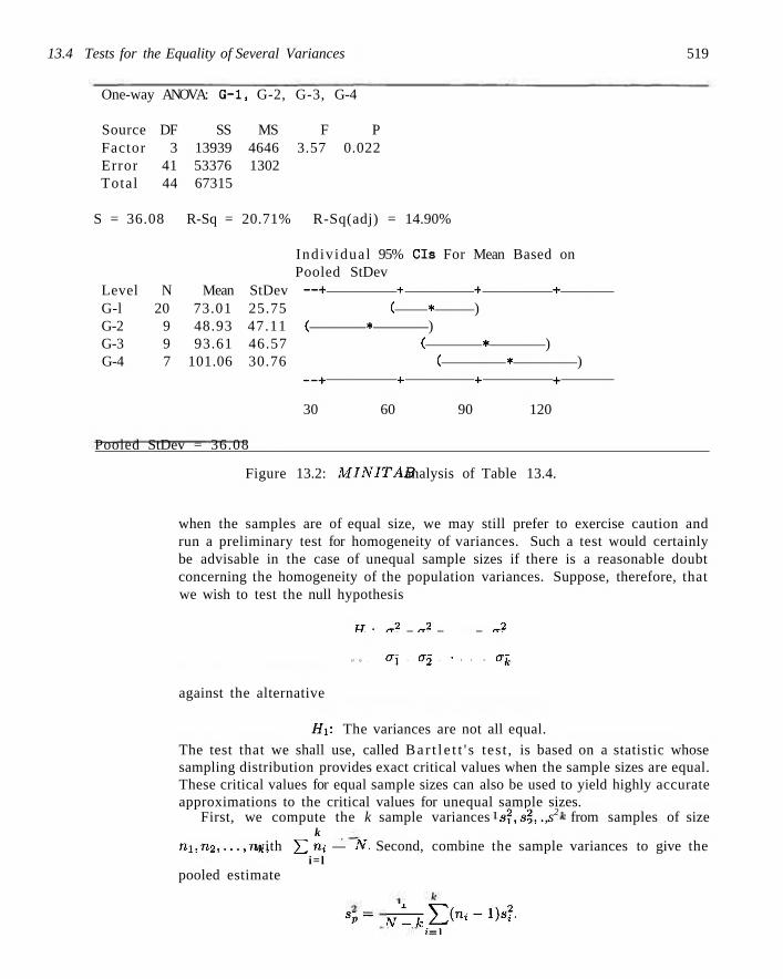
13.4 Tests for the Equality of Several Variances 519
One-way ANOVA: G-l, G-2, G-3, G-4
Source DF SS MS F P Factor 3 13939 4646 3.57 0.022 Error 41 53376 1302 Total 44 67315
S = 36.08 R-Sq = 20.71% R-Sq(adj) = 14.90%
Indiv idual 95% CIs For Mean Based on Pooled StDev
Level N Mean StDev —+ + + + G-l 20 73.01 25.75 ( * ) G-2 9 48.93 47.11 ( * ) G-3 9 93.61 46.57 ( * ) G-4 7 101.06 30.76 ( * )
—+ + + +
30 60 90 120
Pooled StDev = 36.08
Figure 13.2: MINITAB analysis of Table 13.4.
when the samples are of equal size, we may still prefer to exercise caution and run a preliminary test for homogeneity of variances. Such a test would certainly be advisable in the case of unequal sample sizes if there is a reasonable doubt concerning the homogeneity of the population variances. Suppose, therefore, that we wish to test the null hypothesis
W . „2 _ „2 _ _ „2
H Q . O X - a 2 - • • • = a k
against the alternative
Hi: The variances are not all equal.
The test that we shall use, called Ba r t l e t t ' s tes t , is based on a statistic whose sampling distribution provides exact critical values when the sample sizes are equal. These critical values for equal sample sizes can also be used to yield highly accurate approximations to the critical values for unequal sample sizes.
First, we compute the k sample variances s2,s2,.. .,s2 from samples of size k
nx,n2,...,nk, with YI n* — ^- Second, combine the sample variances to give the i= l
pooled estimate
S P = ^ m ^ ( n < - 1 ) ^ ' t•=l

520 Chapter 13 One-Factor Experiments: General
Now
[(^)"--i(^r2-i'--(4)nfc-1]1/(-v-fe)
s2
is a value of a random variable B having the Bartlett distribution. For the special case where m = 712 = • • • = "A- = n, we reject Ho at the o-level of significance if
6< bkia;n),
where 0^(0; n) is the critical value leaving an area of size a in the left tail of the Bartlett distribution. Table A.10 gives the critical values, frfc(a;n), for a = 0.01 and 0.05; k = 2 , 3 , . . . , 10; and selected values of n from 3 to 100.
When the sample sizes are unequal, the null hypothesis is rejected at the o-level of significance if
b< bkia;ni.n2,...,nk),
where
, , v n-xbkia; ni) + n2bk(a; n2) + • • • + nkbk(a;nk) bk(a;ni,n2,...,nk) « r-r •
As before, all the bk(a; m) for sample sizes m , n 2 , . . . , nk are obtained from Table A.10.
Example 13.3:1 Use Bartlett's test to test the hypothesis at the 0.01 level of significance that the population variances of the four drug groups of Example 13.2 are equal.
Solution: Ho'- a2 = a2 = a\ = a\,
Hi: The variances are not equal.
a = 0.01.
Critical region: Referring to Example 13.2, we have n.j = 20, n2 = 9, ri3 = 9, n4 = 7, N = 45, and k = 4. Therefore, we reject when
b < 64(0.01; 20,9,9,7)
_ (20)(0.8586) + (9)(0.6892) + (9)(0.6892) + (7)(0.6045) 45
= 0.7513.
Computations: First compute
s? = 662.862, s\ = 2219.781, s | = 2168.434, s2, = 946.032,
and then
2 _ (19)(662.862) + (8)(2219.781) + (8)(2168.434) + (6)(946.032) SP- 41
= 1301.861.

Exercises 521
Now
b = [(662.862) 19(2219.781)8(2168.434)8(946.032)c]1/41
1301.861 0.8557.
Decision: Do not reject the hypothesis, and conclude that the population variances
of the four drug groups are not significantly different. _l Although Bartlett's test is most often used for testing of homogeneity of vari
ances, other methods are available. A method due to Cochran provides a computationally simple procedure, but it is restricted to situations in which the sample sizes are equal. Cochran's test is particularly useful for detecting if one variance is much larger than the others. The statistic that is used is
G = largest Sf
k '
ESf i-l
and the hypothesis of equality of variances is rejected if g > gQ where the value of ga is obtained from Table A.11.
To illustrate Cochran's test, let us refer again to the data of Table 13.1 on moisture absorption in concrete aggregates. Were we justified in assuming equal variances when we performed the analysis of variance of Example 13.1? We find that
,2 si = 12,134, si = 2303, s^ = 3594, si = 3319, s£ = 3455.
Exercises
Therefore.
12,134 24,805
= 0.4892,
which does not exceed the table value #0.05 = 0.5065. Hence we conclude that the assumption of equal variances is reasonable.
13.1 Show that the mean square error
2 _ SSE 8 - f c ( n - l )
for the analysis of variance in a one-way classification is an unbiased estimate of a2.
13.2 Prove Theorem 13.2.
13.3 Six different machines are being considered for use in manufacturing rubber seals. The machines are being compared with respect, to tensile strength of the product. A random sample of 4 seals from each machine is used to determine whether the mean tensile
strength varies from machine to machine. The following are the tensile-strength measurements in kilograms per square centimeter x 10~':
Machine 1
17.5 16.9 15.8 18.G
2 16.4 19.2 17.7 15.4
3 20.3 15.7 17.8 18.9
4 14.6 16.7 20.8 18.9
5 17.5 19.2 16.5 20.5
6 18.3 16.2 17.5 20.1
Perform the analysis of variance at the 0.05 level of significance and indicate whether or not the mean tensile strengths differ significantly for the 6 machines.
13.4 The data in the following table represent the

522 Chapter 13 One-Factor Experiments: General
number of hours of relief provided by 5 different brands of headache tablets administered to 25 subjects experiencing fevers of 38°C or more. Perforin the: analysis of variance and test the hypothesis at the 0.05 level of significance that, the mean number of hours of relief provided by the tablets is the same for all 5 brands. Discuss the results.
Tablet A 5.2 4.7 8.1 6.2 3.0
B 9.1 7.1 8.2 6.0 9.1
C 3.2 5.8 2.2 3.1 7.2
D 2.4 3.4 4.1 1.0 4.0
E 7.1 6.6 9.3 4.2 7.0
13.5 In an article Shelf-Space Strategy in Retailing, published in the Proceedings: Southern Marketing Association, the effect of shelf height on the supermarket sales of canned dog food is investigated. An experiment was conducted at a small supermarket for a period of 8 days on the sales of a single brand of clog food, referred to as Arf dog food, involving three levels of shelf height: knee level, waist level, and eye level. During each day the shelf height of the canned clog food was randomly changed on three different occasions. The remaining sections of the gondola that housed the given brand were filled with a mixture of dog food brands that were both familiar and unfamiliar to customers in this particular geographic area. Sales, in hundreds of dollars, of Arf dog food per day for the three shelf heights are as follows:
Shelf Height Knee Level Waist Level Eye Level
77 82 86 78 81 86 77 81
88 94 93 90 91 94 90 87
85 85 87 81 80 79 87 93
Is there a significant difference in the average daily sales of this dog food based on shelf height? Use a, 0.01 level of significance.
13.6 Immobilization of free-ranging white-tailed deer by drugs allows researchers the opportunity to closely examine deer and gather valuable physiological information. In the study Influence of Physical. Restraint and Restraint Facilitating Drugs on Blood Measurements of White-Tailed Deer and Other Selected Mammals conducted at the Virginia Polytechnic Institute and State University, wildlife biologists tested the "knockdown" time (time from injection to immobilization) of three different immobilizing drugs. Immobilization, in this case, is defined as the point where the animal no longer has enough muscle control to
remain standing. Thirty male white-tailed deer were randomly assigned to each of three treatments. Group A received 5 milligrams of liquid succinylcholine chloride (SCC); group B received 8 milligrams of powdered SCC; and group C received 200 milligrams of phency-clidine hydrochloride. Knockdown times, in minutes, were recorded here. Perform an analysis of variance at the 0.01 level of significance and determine whether or not the average knockdown time for the 3 drugs is the same.
Group
A ll 5 14 7 10 7 23 4 11 11
B 10 7 16 7 7 5 10 10 6 12
c 4 4 6 3 5 C 8 3 7 3
13.7 It has been shown that the fertilizer magnesium ammonium phosphate, MgNH^POi, is an effective supplier of the nutrients necessary for plant growth. The compounds supplied by this fertilizer are highly soluble in water, allowing the fertilizer to be applied directly on the soil surface or mixed with the growth substrate during the potting process. A study on the Effect, of Magnesium Ammonium Phosphate on Height of Chrysanthemums was conducted at George Mason University to determine a possible optimum level of fertilization, based on the enhanced vertical growth response of the chrysanthemums. Forty chrysanthemum seedlings were divided into 4 groups each containing 10 plants. Each was planted in a similar pot containing a uniform growth medium. To each group of plants an increasing concentration of .\lgNH4PO4, measured in grains per bushel, was added. The 4 groups of plants were grown under uniform conditions in a greenhouse for a period of four weeks. The treatments and the respective changes in heights, measured in centimeters, are shown in the following table:
Treatment 50 g/bu 100 g/bu 200 g/bu 400 g/bu
13.2 12.4 12.8 17.2 13.0 14.0 14.2 21.6 15.0 20.0
16.0 12.6 14.8 13.0 14.0 23.6 14.0 17.0 22.2 24.4
7.8 14.4 20.0 15.8 17.0 27.0 19.6 18.0 20.2 23.2
21.0 14.8 19.1 15.8 18.0 26.0 21.1 22.0 25.0 18.2

13.5 Single-Degree-of-Freedom Comparisons 523
Can wc conclude at the 0.05 level of significance that different concentrations of Mg'NH.iPO.i affect the average attained height of chrysanthemums'' How much Mg'NH.iPO.i appears to be best?
13.8 A study measures the sorption (either absorption or adsorption) rate of three different types of organic chemical solvents. These solvents are used to clean industrial fabricated-metal parts and are potential hazardous waste. Independent samples of solvents from each type were tested and their sorption rates were recorded as a mole percentage. [See McClave, Dietrich, and Sincich (1997).]
Aroma t i c s 1.06 0.95 0.79 0.65 0.82 1.15 0.89 1.12 1.05
Chloroalkanes 1.58 1.12 1.45 0.91 0.57 0.83 1.16 0.43
0.29 0.06 0.44 0.55 0.61
Esters 0.43 0.51 0.10 0.53 0.34
0.06 0.09 0.17 0.17 0.60
Is there a significant difference in the mean sorption rate for the three solvents? Use a P-value for your conclusions. Which solvent would you use?
13.9 The mitochondrial enzyme NAPH:NAD tran-shydrogenase of the common rat tapeworm (lly-menolepiasis diminuta) catalyzes hydrogen in transfer from NADYH to NAD, producing NADH. This enzyme is known to serve a vital role in the tapeworm's anaerobic metabolism, and it has recently been hypothesized that it may serve as a proton exchange pump, transferring protons across the mitochondrial
membrane. A study on Effect of Various Substrate Concentrations on the Conformational Variation of the, NADPII:NAD Transhydrogenase of Hymenolepia-sis diminutaconducted at Bowling Green State: University was designed to assess the ability of this enzyme to undergo conformation or shape changes. Changes in the specific activity of the enzyme caused by variations in the concentration of NADP could be interpreted as supporting the theory of conformational change. The enzyme in question is located in the inner membrane of the tapeworm's mitochondria. These tapeworms were homogenized, and through a series of centrifugations, the enzyme was isolated. Various concentrations of NADP were then added to the isolated enzyme solution, and the mixture was then incubated in a water bath at 56°C for 3 minutes. The enzyme was then analyzed on dualbeam spectrophotometer, and the following results were calculated in terms of the specific activity of the: enzyme in nanomoles per minute per milligram of protein:
N A D P Concen t r a t i on (ran) 0
11.01 12.09 10.55 11.26
80 11.38 10.07 12.33 10.08
160 11.02 10.67 11.50 10.31
360 6.04 10.31 8.65 8..'it) 7.76 9.48
10.13 8.89 9.36
Test the hypothesis at the 0.01 level that the: average specific activity is the same for the four concentrations.
13.10 For the data set in Exercise 13.7, use Bartlett's test to check whether the variances are equal.
13.5 Single Degree of Freedom Comparisons
The analysis of variance in a one-way classification, or tho one-factor experiment, as it, is often called, merely indicates whether or not the hypothesis of equal t reatment means can be rejected. Usually, an experimenter would prefer his or her analysis to probe deeper. For instance, in Example 13.1, by rejecting the null hypothesis we concluded tha t the means are not all equal, but we still do not know where the differences exist among the aggregates. The engineer might have the- feeling a priori t h a t aggregates 1 and 2 should have similar absorption properties and tha t the same is t rue for aggregates 3 and 5. However, it is of interest to s tudy the difference between the two groups. It would seem, then, appropriate to test the hypothesis
H 0 : px +fi2 - / / / j
Hi: pi + ft2 - //,!
- M6 = 0,
- pr, ? 0.
We notice that the hypothesis is a linear function of the population means where the coefficients sum to zero.

524 Chapter 13 One-Factor Experiments: General
Definition 13.1: Any linear function
k
where YI Ci = 0 , is i = i
of the form
k
t = i
called a comparison
Pi,
or contrast in the treatment means.
The experimenter can often make multiple comparisons by testing the significance of contrasts in the treatment means, that is, by testing a hypothesis of the type
Hypothesis for a Contrast HQ: 22 c*A*j = 0,
i = l
k
Hi: Y^ ciP-i ¥> °i ( = i
where YI ci — 0. » = i
The test is conducted by first computing a similar contrast in the sample means,
fc '«•' = ^Cilji..
i-l
Since Y\,,Y2.,... ,Yk. are independent random variables having normal distributions with means p.i,p.2,...,pk and variances a2/nx,o2/n2,... ,o2/nk, respectively, Theorem 7.11 assures us that w is a value of the normal random variable W with mean
Pw = 22 CiP{
i=i
and variance
J2 _ _2 V ^ Ci
i = l
Therefore, when HQ is true, u\y = 0 and, by Example 7.5, the statistic
W2 £ ciY. i = i
°w *2£(c?M) i=X
is distributed as a chi-squared random variable with 1 degree of freedom. Our hypothesis is tested at the o-level of significance by computing

13.5 Single-Degree-of-Freedom Comparisons 525
Test Statistic for Testing a Contrast
YH^/m) :i=X
Definition 13.2:
f £ Civ,.
s2Zic2/n,) S2 £ ( c ? / n 0
i= l i-\
SSw
Here / is a value of the random variable F having the F-distribution with 1 and Ar — k degrees of freedom.
When the sample sizes are all equal to n, 2
SSw = kc'n)' t = l
The quantity SSw, called the contrast sum of squares, indicates the portion of SSA that is explained by the contrast in question.
This sum of squares will be used to test the hypothesis that the contrast
k
^ dpi = 0. 7 = 1
It is often of interest to test multiple contrasts, particularly contrasts that are linearly independent or orthogonal. As a result, we need the following definition:
The two contrasts
wi = \V2 biPi and ^ 2 = ^ CiPi
i=X t = l
are said to be orthogonal if £ biCi/n, = 0 or, when the n;'s arc all equal to n, i-l
if
^ f c ; c ; = 0. ; = i
If W] and LJ2 are orthogonal, then the quantities 55u'i and SSw2 are components of 55.4, each with a single degree of freedom. The treatment sum of squares with A: — 1 degrees of freedom can be partitioned into at most A: — 1 independent single-degrec-of-freedom contrast sum of squares satisfying the identity
SSA = SSwi + SSw2 + ••• + SSwk-i,
if the contrasts are orthogonal to each other.
Example 13.4:1 Referring to Example 13.1, find the contrast sum of squares corresponding to the orthogonal contrasts
Wi = fix + fl2 - p3 - P5, U>2 = pi+ fi2 + ps - 4u4 + fl-5,
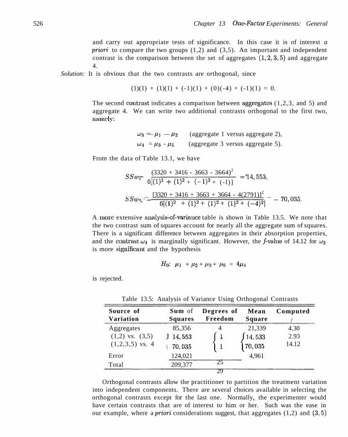
526 Chapter 13 One-Factor Experiments: General
and carry out appropriate tests of significance. In this case it is of interest a priori, to compare the two groups (1,2) and (3,5). An important and independent contrast is the comparison between the set of aggregates (1,2,3,5) and aggregate 4.
Solution: It is obvious that the two contrasts are orthogonal, since
(1)(1) + (1)(1) + (-1)(1) + (0)(-4) + (-1)(1) = 0.
The second contrast indicates a comparison between aggregates (1,2,3, and 5) and aggregate 4. We can write two additional contrasts orthogonal to the first two, namely:
w.3 — IH — P2 (aggregate 1 versus aggregate 2),
OJ4 = p-i - Pb (aggregate 3 versus aggregate 5).
From the data of Table 13.1, we have
(3320 + 3416 - 3663 - 3664)2 1 , r r o
SSWi = 6[(l)» + (l)* + ( - l )» + ( - l ) ] = M ' d d 3 :
_ [3320 + 3416 + 3663 + 3664 - 4(2791)]2 _ A " " Q[(l)2 + (l)2 + (l)2 + (l)2 + (-4y\ ~ W^°-
A more extensive analysis-of-variance table is shown in Table 13.5. We note that the two contrast sum of squares account for nearly all the aggregate sum of squares. There is a significant difference between aggregates in their absorption properties, and the contrast U/'i is marginally significant. However, the /-value of 14.12 for u}2
is more significant and the hypothesis
HQ: px + p2 + p3 + (is = 4p4
is rejected.
Table 13.5: Analysis of Variance Using Orthogonal Contrasts
Source of Variation Aggregates (1,2) vs. (3,5) (1,2,3,5) vs. 4
Error Total
Sum of Squares
85,356 J 14,553 \ 70,035
124,021 209,377
Degrees of Freedom
4
l: 25 29
Mean Square 21,339
J14,533 j70,035
4,961
Computed /
4.30 2.93
14.12
Orthogonal contrasts allow the practitioner to partition the treatment variation into independent components. There are several choices available in selecting the orthogonal contrasts except for the last one. Normally, the experimenter would have certain contrasts that are of interest to him or her. Such was the ease in our example, where a priori considerations suggest, that aggregates (1,2) and (3,5)

13.6 Multiple Comparisons 527
constitute distinct groups with different absorption properties, a postulation that was not strongly supported by the significance test. However, the second comparison supports the conclusion that aggregate 4 seems to ilstand out" from the rest. In this case the complete partitioning of 55.4 was not necessary, since two of the four possible independent comparisons accounted for a majority of the variation in treatments.
Figure: 13.3 shows a 5.45 GLM procedure that displays a complete set of orthogonal contrasts. Note that the sum of squares for the four contrasts adds to the aggregate sum of squares, Also, that the latter two contrasts (1 versus 2, 3 versus 5) reveal insignificant comparisons. J
Dependent Variable
Source
Model Error
Corrected
R-0.
Source
aggregate
Source
aggregate
Contrast
(1,2,3,5)
(1,2) vs.
1 vs. 2
3 vs. 5
Total
-Square
.407669
vs. 4
(3,5)
The GLM Procedure
: moisture
DF 4 25 29
C
DF 4
DF 4
DF 1 1 1 1
Sum of Squares
85356.4667
124020.3333 209376.8000
loeff Var
12.53703
Type I SS
85356.46667
Type III SS
85356.46667
Contrast SS
70035.00833
14553.37500
768.00000
0.08333
Mean Square F
21339.1167 4960.8133
Value Pr > F 4.30 0.0088
Root MSE moisture Mean
70.43304
Mean Square
21339.11667
Mean Square
21339.11667
Mean Square
70035.00833
14553.37500
768.00000 0.08333
561.8000
F Value
4.30
F Value
4.30
F Value
14.12
2.93
0.15
0.00
Pr > F
0.0088
Pr > F
0.0088
Pr > F
0.0009
0.0991
0.6973
0.9968
Figure 13.3: A set of orthogonal procedures
13.6 Multiple Comparisons
The analysis of variance is a powerful procedure for testing the homogeneity of a set of means. However, if we reject the null hypothesis and accept the stated alternative that the means are not all equal wc still do noi know which of the population means are equal and which arc different.
In Section 13.5 we describe the use of orthogonal contrasts to make comparisons among sets of factor levels or treatments. The: notion of orthogonality allows the analyst to make tests involving independent contrasts. Thus the variation

528 Chapter 13 One-Factor Experiments: General
among treatments, 55/1, can be partitioned into single-degree-of-freedom components, and then proportions of this variation can be attributed to specific contrasts. However, there are situations in which the use of contrasts is not an appropriate approach. Often it is of interest to make several (perhaps all possible) paired comparisons among the treatments. Actually, a paired comparison may be viewed as a simple contrast, namely, a test of
H0: fn - p.j = 0,
Hf. pi - p.j ji 0,
for all i 7 j. All possible paired comparisons among the means can be very beneficial when particular complex contrasts are not known a priori. For example, in the aggregate data of Table 13.1, suppose that we wish to test
HQ: pi - u$ = 0,
Hi: pi - ps 7^0,
The test is developed through use of an F, t, or a confidence interval approach. Using the t. we have
where s is the square root of the mean square error and n = 6 is the sample size per treatment, In this case
553.33-610.67 , „ t = — . = -1 .41 .
^/4lm^Sl/3 The P-value for the <-test with 25 degrees of freedom is 0.17. Thus there is not sufficient evidence to reject HQ.
Relationship between t and F
In the foregoing we displayed the use of a pooled t-test along the lines of that discussed in Chapter 10. The pooled estimate comes from the mean square error in order to enjoy the degrees of freedom that are pooled across all five samples. In addition, we have tested a contrast. The reader should note that if the lvalue is squared, the result is exactly of the form of the value of / for a test on a contrast discussed in the preceding section. In fact,
, _ im.-Vs.)2 __ (553.33-610.67)2
1 *2(l/6 + l/6) 4961(1/3) '
which, of course, is t2.
Confidence Interval Approach to a Paired Comparison
It is straightforward to solve the same problem of a paired comparison (or a contrast) using a confidence interval approach. Clearly, if we compute a 100(1 — o)%

13.6 Multiple Comparisons 529
confidence interval on pi — p$, we have
Si. -So . ±tD t«/2S\j-,
where tn/2 is the upper 100(1 - a/2)% point of a /.-distribution with 25 degrees of freedom (degrees of freedom coming from s2). This straightforward connection between hypothesis testings and confidence intervals should be obvious from discussions in Chapters 9 and 10. The test of the simple contrast u-x - Po involves no more than observing whether or not the confidence interval above covers zero. Substituting the numbers, we have as the 95% confidence interval
(553.33 - 610.67) ± 2.060\/496Ti/i = -57.34 ± 83.77.
Thus, since the interval covers zero, the contrast is not significant. In other words, we do not. find a significant difference between the means of aggregates 1 and 5.
Experiment-Wise Error Rate
Tukey's Test
We have demonstrated that a simple contrast (i.e., a comparison of two means) can be made through an F-test as demonstrated in Section 13.5, a i-test, or by computing a confidence interval on the difference between the two means. However, serious difficulties occur when the analyst attempts to make many or all possible paired comparisons. For the case of k means, there will be, of course, r — k(k — l ) /2 possible paired comparisons. Assuming independent comparisons, the experiment-wise error rate (i.e., the probability of false rejection of at least one of the hypotheses) is given by 1 — (1 — a)r, where a is the selected probability of type I error for a specific comparison. Clearly, this measure of experiment-wise type I error can be quite large. For example, even if there are only 6 comparisons, say, in the case of 4 means, and o = 0.05, the experiment-wise rate is
1 - (0.95)6 ss 0.26.
With the task of testing many paired comparisons there is usually the need to make the effective contrast on a single comparison more conservative. That is, using the confidence interval approach, the confidence intervals would be much wider than the ±ta/2s\/2/n used for the case where only a single comparison is being made.
There are several standard methods for making paired comparisons that sustain the credibility of the type I error rate. We shall discuss and illustrate two of thern here. The first one, called Tukey's procedure, allows formation of simultaneous 100(1 — a)% confidence intervals for all paired comparisons. The method is based on the studentized range distribution. The appropriate percentile point is a function of a, k, and v = degrees of freedom for s2. A list of upper percentage points for Q = 0.05 is shown in Table A. 12. The method of paired comparisons by Tukey involves finding a significant difference between means i and j (i ^ j) if |jfe. — y~jm\
exceeds 17(0-, k, v] J -.

530 Chapter 13 One-Factor Experiments: General
Tukey's procedure is easily illustrated. Consider a hypothetical example where we have 6 treatments in a one-factor completely randomized design with 5 observations taken per treatment. Suppose that the mean square error taken from the analysis-of-variance table is s2 = 2.45 (24 degrees of freedom). The sample means are in ascending order.
])2. Vo. Vi. V'i. Ve. VA.
14.50 16.75 19.84 21.12 22.90 23.20.
With a = 0.05, the value of <7(0.05,6,24) = 4.37. Thus all absolute differences arc-to be compared to
4 . 3 7 1 / - ^ = 3.059.
As a result, the following represent moans found to be significantly different using Tukey's procedure:
4 and 1, 4 and 5, 4 and 2, 6 and 1, 6 and 5, 6 and 2, 3 and 5, 3 and 2, 1 and 5, 1 and 2.
Where Does the a-Level Come from in Tukey's Test?
We briefly alluded to the concept of s imultaneous confidence intervals that arc employed for Tukey's procedure. The reader will gain a useful insight into the notion of multiple comparisons if he or she gains an understanding of what is meant by simultaneous confidence intervals.
In Chapter 9 we learned that if we compute a confidence interval on, say, a mean p, then the probability that the interval covers the true mean p is 0.95. However, as we have discussed for the case of multiple comparisons, the effective probability of interest is tied to the experiment-wise error rate and it should be emphasized that the confidence intervals of the type y,. — fjj. ± q[a, k, v]sy/l/n are not independent since they all involve s and many involve the use of the same averages, the pi,. Despite the difficulties, if we use the q(0.05. k,v), the simultaneous confidence level is controlled at 95%. The same holds for q(0.01, k, v), namely the confidence level is controlled at 99%. In the case of a = 0.05, there is a probability of 0.05 that at least one pair of measures will be falsely found to be different (false rejection of at least one hypothesis). In the a = 0.01 case the corresponding probability will be 0.01.
Duncan's Test The second procedure we shall discuss is called Duncan's procedure or Duncan's multiple-range test. This procedure is also based on the general notion of studentized range. The range of any subset of p sample means must exceed a certain value before any of the p means are found to be different. This value is called the least significant range for the p means and is denoted as Rp, where

13.7 Comparing Treatments with a Control 531
The values of the quantity rp, called the1 least significant s tudent ized range, depend on the desired level of significance and the number of degrees of freedom of the mean square error. These values may be obtained from Tabic A.13 for p = 2 , 3 , . . . 11.0 means.
To illustrate the multiple-range test procedure, let us consider the hypothetical example where G treatments are compared with 5 observations per treatment. This is the same example as that used to illustrate Tukey's test. We obtain R.v by multiplying each rp by 0.70. The results of these computations are summarized as follows:
V
l'l>
2
2.919 2.043
3
3.06G 2.146
1
3.160 2.212
5
3.226 2.258
6
3.276 2.293
Comparing these least: significant ranges with the differences in ordered means, we arrive at the following conclusions:
1. Since v/4. — f/2. = 8.70 > /?Q = 2.293, we conclude: that //,[ and p2 are significantly differenl.
2. Comparing y4, - 1/5. and i/,;. — y2, with /?.-,, we conclude that ft,\ is significantly greater than fir, and fio is significantly greater than p2.
3. Comparing y4, — yi., j/y. — j/5., and y-j, — y2. with R4, wc conclude that each difference is significant.
4. Comparing j/4, — y-.i,. yo, — yi,, fj-.i. — v/r,., and 1/1. — [/•>. with R.-.i, we find all differences significant except for m — p3. Therefore, fi3, p4, and po constitute a subset of homogeneous means.
5. Comparing y:!. - [/],. yi, — yr,., and §5. — S2. with R2- wc conclude that only ps and ft-i are not significantly different.
It is customary to summarize the conclusions above by drawing a lino under any subset of adjacent means that are not significantly different. Thus wc have
in. TJTJ. S I . S3. Se. Vi. 14.50 16.75 19.84 21.12 22.90 23.20
It is clear that in this case the results from Tukey's and Duncan's procedures are very similar. Tukey's procedure did not detect a difference between 2 and 5, whereas Duncan's did.
13.7 Comparing Treatments with a Control
In many scientific and engineering problems one is not interested in drawing inferences regarding' all possible comparisons among the treatment means of the type Pi — fij. Rather, the experiment often dictates the need for comparing simultaneously each treatment with a control. A test procedure developed by C. W. Dunnett determines significant differences between each treatment mean and the control, at a single joint, significance level a. To illustrate Dunnett's procedure, let us consider the experimental data of Tabic 13.6 for the one-way classification where the effect

532 Chapter 13 One-Factor Experiments: General
Table 13.6: Yield of Reaction
Control 50.7 51.5 49.2 53.1 52.7
So. = 51.44
Catalyst 1
Si.
54.1 53.8 53.1 52.5 54.0
= 53.50
Catalyst 2
S2.
52.7 53.9 57.0 54.1 52.5
= 54.04
Catalyst 3
2/3
51.2 50.8 49.7 48.0 47.2
= 49.38
of three catalysts on the yield of a reaction is being studied. A fourth treatment, no catalyst, is used as a control.
In general, wc wish to test the k hypotheses
Ho- Po = pA i = 1 ) 2 ) . . . ) j f c ) Hi: po^Pi)
where po represents the mean yield for the population of measurements in which the control is used. The usual analysis-of-variance assumptions, as outlined in Section 13.3, are expected to remain valid. To test the null hypotheses specified by Ho against two-sided alternatives for an experimental situation in which there are A: treatments, excluding the control, and n observations per treatment, we first calculate the values
, Vi. - SO. . - i n I, di = —; , t = 1,2,...,K.
y/2^Jn The sample variance s2 is obtained, as before, from the mean square error in the analysis of variance. Now, the critical region for rejecting Ho, at the a-level of significance, is established by the inequality
\di\ > da/2(k,v),
where v is the number of degrees of freedom for the mean square error. The values of the quantity dn/2(k, v) for a two-tailed test are given in Table A. 14 for o = 0.05 and a = 0.01 for various values of k and v.
Example 13.5:1 For the data of Table 13.6, test hypotheses comparing each catalyst with the control, using two-sided alternatives. Choose a = 0.05 as the joint significance level.
Solution: The mean square error with 16 degrees of freedom is obtained from the analysis-of-variance table, using all k + 1 treatments. The mean square error is given by
, 36.812 s2 = —— = 2.30075,
16
and
m?om=0i9593>

Exercises 333
Hence
, 5 3 . 5 0 - 5 1 . 4 4 (h= 0.9593 =2M'<
«fe- 5 4 - ° 4 - . 5 . 1 - 4 4 = 2.710, 0.9593
49.38 - 51.44 -2.147.
0.9593
From Table A. 14 the critical value for a = 0.05 is found to be
do.025(3,16) = 2.59.
Since \dx\ < 2.59, and \d3\ < 2.59, wc conclude that only the mean yield for catalyst
2 is significantly different from the mean yield of the reaction using the control. J Many practical applications dictate the need for a one-tailed test for comparing
t reatments with a control. Certainly, when a pharmacologist is concerned with the comparison of various dosages of a drug on the effect, of reducing cholesterol level, and his control is zero dosage, it. is of interest to determine if each dosage produces a significantly larger reduction than that of the control. Table A. 15 shows the critical values o{d„(k,v) for one-sided alternatives.
Exercises
13.11 Consider the data of Review Exercise 13.58 on page 568. Make significance tests on the following contrasts:
(a) B versus A, C, and D;
(b) C versus A and D\
(c) A versus D.
13.12 The study Loss of Nitrogen Through Sweat by Preadolescent Boys Consuming Three Levels of Dietary Protein was conducted by the Department of Human Nutrition and Foods at the Virginia Polytechnic Institute and State University to determine perspiration nitrogen loss at, various dietary protein levels. Twelve preadolescent boys ranging in age from 7 years, 8 months to !) years, 8 months, and judged to be clinically healthy, were used in the experiment. Each boy was subjected to one of three controlled diets in which 29. 54, or 84 grams of protein per day were: consumed. The following data represent, the body perspiration nitrogen loss, in milligrams, collected during the last two days of the experimental period:
P r o t e i n Level 29 G r a m s
190 266 270
54 G r a m s 318 295 271 438
84 G r a m s 390 321 390 399
(a) 402
Perform an analysis of variance at the 0.05 level of significance: to show that the mean perspiration nitrogen losses at the three protein levels arc different. Use a single' degree-of-freedom contrast with a = 0.05 to compare the mean perspiration nitrogen loss for boys who consume 29 grams of protein per day versus boys who consume 54 and 84 grams of protein.
13.13 The purpose of the study The Incorporation of a. Chelating Agent into a Flame Retardant Finish of a Cotton Flannelette and the Evaluation of Selected Fabric Properties conducted at the Virginia Polytechnic Institute and State University was to evaluate: the use of a chelating agent as part of the flamc-ictardant finish of cotton flannelette by determining its effects upon

534 Chapter 13 One-Factor Experiments: General
flammability after the fabric is laundered under specific conditions. Two baths were prepared, one with car-boxyinethyl cellulose and one without. Twelve pieces of fabric were laundered 5 times in bath I, and 12 other pieces of fabric were laundered 10 times in bath I. This was repeated using 24 additional pieces of cloth in bath II. After the washings the lengths of fabric: that burned and the burn times were measured. For convenience, let us define the following treatments:
Treatment 1: 5 launderings in bath I,
Treatment 2: 5 launderings in bath II,
Treatment 3: 10 launderings in bath I,
Treatment 4: 10 launderings in bath II.
Burn times, in seconds, were recorded as follows:
Treatment
Blend
1 13.7 23.0 15.7 25.5 15.8 14.8 14.0 29.4 9.7
14.0 12.3 12.3
2 6.2 5.4 5.0 4.4 5.0 3.3
16.0 2.5 1.6 3.9 2.5 7.1
3 27.2 16.8 12.9 14.9 17.1 13.0 10.8 13.5 25.5 14.2 27.4 11.5
4 18.2 8.8
14.5 14.7 17.1 13.9 10.6 5.8 7.3
17.7 18.3 9.9
(a) Perforin an analysis of variance using a 0.01 level of significance and determine whether there are any significant differences among the treatment means.
(b) Use single-degree-of-freedom contrasts with a = 0.01 to compare the mean burn time of treatment 1 versus treatment 2 and also treatment 3 versus treatment 4.
13.14 Use Tukey's test, with a 0.05 level of significance, to analyze the means of the 5 different brands of headache tablets in Exercise 13.4 on page 521.
13.15 For the data used in Review Exercise 13.58 on page 568, perform Tukey's test with a 0.05 level of significance to determine which laboratories differ, on average, in their analysis.
13.16 An investigation was conducted to determine the source of reduction in yield of a certain chemical product. It was known that the loss in yield occurred in the mother liquor, that is. the material removed at the filtration stage. It was felt that different blends of the original material may result in different yield reductions at the mother liquor stage. The following are results of the percent reduction for 3 batches at each of 4 preselected blends:
25.0 24.3 27.9
25.2 28.6 24.7
20.8 26.7 22.2
31.6 29.8 34.3
(a) Perform the analysis of variance at the a = 0.05 level of significance.
(b) Use Duncan's multiple-range test to determine which blends differ.
(c) Do part, (b) using Tukey's test.
13.17 In the study An Evaluation of the Removal Method for Estimating Benthic Populations and Diversity conducted by the Virginia Polytechnic Institute and State University on the Jackson River, 5 different sampling procedures were used to determine the species count. Twenty samples were selected at random and each of the 5 sampling procedures were repeated 4 times. The species counts were recorded as follows:
Sampling Procedure
Depletion 85 55 40 77
Modified Hess
75 45 35 67
Surber 31 20 9
37
Substrate Removal Kick-Kicknet net
43 17 21 10 15 8 27 15
(a) Is there a significant difference in the average species count for the different sampling procedures? Use a P-value in your conclusion.
(b) Use Tukey's test with a = 0.05 to find which sampling procedures differ.
13.18 The following data are values of pressure (psi) in a torsion spring for several settings of the angle be-tween the legs of the spring in a free position:
Angle (°) 67 83 85
71 84 85 85 86 86 87
75 86 87 87 87 88 88 88 88 88 89 90
79 89 90 90 91
83 90 92
Compute a one-way analysis of variance for this experiment and state your conclusion concerning the effect of angle on the pressure in the spring. (C. R. Hicks, Fundamental Concepts in the Design of Experiments, Holt, Rinebart and Winston, New York, 1973.)
13.19 In the following biological experiment 4 concentrations of a certain chemical are used to enhance the growth of a certain type of plant over time. Five
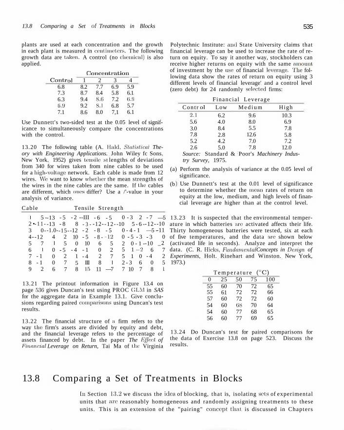
13.8 Comparing a Set of Treatments in Blocks 535
plants are used at each concentration and the growth in each plant is measured in centimeters. The following growth data are taken. A control (no chemical) is also applied.
Concen t r a t i on Con t r
6.8 7.3 6.3 0.9 7.1
ol 1 8.2 8.7 9.4 9.2 8.6
2 7.7 8.4 8.6 8.1 8.0
3 6.9 5.8 7.2 6.8 7,1
4 5.9 6.1 ( i . ' . i
5.7 6.1
Use Dunnett's two-sided icance to simultaneously with the control.
test at the 0.05 level of signif-compare the concentrations
13.20 The following table (A. Ilald, Statistical. Theory with Engineering Applications. John Wiley fc Sons. New York. 1952) gives tensile1 si lengths of deviations from 340 for wires taken from nine cables to be used for a high-voltage network. Each cable is made from 12 wires. We want to know whether the mean strengths of the wires in the nine cables are the same. If the cables are different, which ones differ? Use a /'-value in your analysis of variance.
Cable Tensile S t r e n g t h
1 2 • 3 4-5 6 7 8 9
5 -- 1 1 -
0--12
7 1
- 1 - 1
2
-13 -13 -1.0-
4 1 0 0 0 6
- 5 - 8 -15-
2 5
- 5 2 7 7
- 2 -8
-12 10 0
- 4 I 5 8
-III - 3 -- 2 - 5 10
- 1 - 4 III 15
- 6 -12-- 8 - 8 -
6 0 2 8
11
- 5 -12 -- 5 -12
5 2 7 1
—7
0 - 3 2 -10 5 - 6 -
0 - 4 - 1 0 - 5 - 3 2 0 - 1 -5 1 - 2 5 1 0 2 - 3 6 7 10 7
- 7 -12-—5 -- 3
-10 6
- 4 0 8
—5 -10 -11
0 _2
7 2 5 I
13.21 The printout information in Figure 13.4 on page 530 gives Duncan's test using PROC GLM in SAS for the aggregate data in Example 13.1. Give conclusions regarding paired comparisons using Duncan's test results.
13.22 The financial structure of a firm refers to the way the firm's assets are divided by equity and debt, and the financial leverage refers to the percentage of assets financed by debt. In the paper The Effect of Financial Leverage on Return, Tai Ma of the Virginia
Polytechnic Institute: and State University claims that financial leverage can be used to increase the rate of return on equity. To say it another way, stockholders can receive higher returns on equity with the same amount, of investment by the use: of financial leverage. The following data show the rates of return on equity using 3 different levels of financial leverage' and a control level (zero debt) for 24 randomly selected firms:
F inanc ia l Leverage Con t r
2.1 5.6 3.0 7.8 5.2 2.6
ol Low 6.2 4.0 8.4 2.8 4.2 5.0
M e d i u m 9.6 8.0 5.5
12.6 7.0 7.8
High 10.3 6.9 7.8 5.8 7.2
12.0 Source: Standard & Poor's Machinery Industry Survey, 1975.
(a) Perform the analysis of variance at the 0.05 level of significance. Use Dunnett's test at the 0.01 level of significance to determine whether the mean rates of return on equity at the low, medium, and high levels of financial leverage are higher than at the control level.
(b
13.23 It is suspected that the environmental temperature in which batteries are: activated affects their life. Thirty homogeneous batteries were tested, six at each of five temperatures, and the data are shown below (activated life in seconds). Analyze and interpret the data. (C. R. Hicks, Fundamental Concepts in Design, of Experiments, Holt. Rinehart and Winston. New York, 1973.)
T e m p e r a t u r e (°C) 0 55 55 57 54 54 56
25 60 61 60 60 60 60
50 70 72 72 08 77 77
75 72 72 72 70 68 69
100 65 66 60 64 65 65
13.24 Do Duncan's test for paired comparisons for the data of Exercise 13.8 on page 523. Discuss the results.
13.8 Comparing a Set of Treatments in Blocks
In Section 13.2 we discuss the idea of blocking, tha t is, isolating sets of experimental units that arc reasonably homogeneous and randomly assigning t reatments to these units. This is an extension of the "pairing" concept that is discussed in Chapters

536 Chapter 13 One-Factor Experiments: General
The GLM Procedure Duncan's Multiple Range Test for moisture
NOTE: This t e s t cont ro l s the Type I comparisonwise e r ro r r a t e , not the experimentwise e r ro r r a t e .
Alpha 0.05 Error Degrees of Freedom 25 Error Mean Square 4960.813
Number of Means 2 3 4 5 C r i t i c a l Range 83.75 87.97 90.69 92.61
Means with the same l e t t e r a re not s i g n i f i c a n t l y d i f f e r e n t . Duncan Grouping Mean N aggregate
A 610.67 6 5 A A 610.50 6 3 A A 569.33 6 2 A A 553.33 6 1
B 465.17 6 4
Figure 13.4: SAS printout for Exercises 13.21.
9 and 10 and is done to reduce experimental error, since the units in blocks have characteristics that are more common than units that are in different blocks.
The reader should not view blocks as a second factor, although this is a tempting way of visualizing the design. In fact, the main factor (treatments) still carries the major thrust of the experiment. Experimental units are still the source of error, just as in the completely randomized design. We merely treat sets of these units more systematically when blocking is accomplished. In this way, we say there are restrictions in randomization. For example, for a chemical experiment designed to determine if there is a difference in mean reaction yield among four catalysts, samples of materials to be tested are drawn from the same batches of raw materials, while other conditions, such as temperature and concentration of reactants, are held constant. In this case the time of day for the experimental runs might represent the experimental units, and if the experimenter feels that, there could possibly be a slight time effect, he or she would randomize the assignment of the catalysts to the runs to counteract the possible trend. This type of experimental strategy is the completely randomized design. As a second example of such a design, consider an experiment to compare four methods of measuring a particular physical property of a fluid substance. Suppose the sampling process is destructive; that is, once a sample of the substance has been measured by one method, it cannot be measured again by any of the other methods. If it is decided that 5 measurements are to be taken for each method, then 20 samples of the material are selected from a large

13.9 Randomized Complete Block Designs 537
batch at random and are used in the experiment to compare the four measuring devices. The experimental units are the randomly selected samples. Any variation from sample to sample will appear in the error variation, as measured by s2 in the analysis.
What Is the Purpose of Blocking4!
If the variation due to heterogeneity in experimental units is so large that the sensitivity of detecting treatment differences is reduced due to an inflated value of s2, a better plan might be to "block off" variation due to these units and thus reduce the extraneous variation to that accounted for by smaller or more homogeneous blocks. For example, suppose that in the previous catalyst illustration it is known a priori that there definitely is a significant, day-to-day effect on the yield and that we can measure the yield for four catalysts on a given day. Rather than assign the 4 catalysts to the 20 test runs completely at random, we choose, say, 5 days and run each of the 4 catalysts on each day, randomly assigning the catalysts to the runs within days. In this way the day-to-day variation is removed in the analysis and consequently the experimental error, which still includes any time trend within days, more accurately represents chance variation. Each day is referred to as a block.
The most straightforward of the randomized block designs is one in which we randomly assign each treatment, once to every block. Such an experimental layout is called a randomized complete block design, each block constituting a single replication of the treatments.
13.9 Randomized Complete Block Designs
A typical layout for the randomized complete block design (RCB) using 3 measurements in 4 blocks is as follows:
Block 1 Block 2 Block 3 Block 4
t2
u h
tx h t2
t3
t2
tx
t2
tx h
The t's denote the assignment to blocks of each of the 3 treatments. Of course, the true allocation of treatments to units within blocks is done at random. Once the experiment has been completed, the data can be recorded as in the following 3 x 4 array:
Treatment 1 2 3
Block: 1
Vn J/21
2/31
2
2/12
2/22
2/32
3
2/13
2/23
2/33
4
2/14
2/24
J/34
where yn represents the response obtained by using treatment 1 in block 1, yi2
represents the response obtained by using treatment 1 in block 2, . . . , and y34
represents the response obtained by using treatment 3 in block 4.

538 Chapter 13 One-Factor Experiments: General
Let us now generalize and consider the case of k treatments assigned to b blocks. The data may be summarized as shown in the k x b rectangular array of Table 13.7. It will be assumed that the y^, i = 1, 2 , . . . , k and j = 1,2,..., b, are values of independent random variables having normal distributions with means p-ij and common variance a2.
Table 13.7: k x b Array for the RCB Design
Treatment
1 2
1
2/ii
2/21
2
J/12
2/22
Block: j
... yij ..
... y2j . .
6
V2b
T o t a l
Ti.
T-2.
M e a n
2/i. y-2.
yn yt2 ••• yu • • • y*b T.
k
Total
Mean
2/fci
Ti
V-i
2/fc2 T2 ..
y.2 ••
' 2/fej '
• T.j ••
• v., •
ykb
•• T.b
•• y.b
Tk.
T. Vk.
V-
Let pi. represent the average (rather than the total) of the b population means for the ith treatment. That is,
1 b
^-= 1^2^' j=X
Similarly, the average of the population means for the j th block, p.j, is defined by
1 k
i=\
and the average of the bk population means, u, is defined by
1 k b
^=^EE^-»=i j = i
To determine if part of the variation in our observations is due to differences among the treatments, we consider the test
Hypothesis of ttment Means Hx: The /Zj.'s are not all equal.
Equal Treatment H*' (l1- ~ f'2- **»
Model for the RCB Design
Each observation may be written in the form
Vij — Pij + eij)

13.9 Randomized Complete Block Designs 539
where e-,j measures the deviation of the observed value yy from the population mean pij. The preferred form of this equation is obtained by substituting
Pij = p + ai + 0j,
where ct< is, as before, the effect of the ith treatment and 3j is the effect of the j t h block. It is assumed that the treatment and block effects are additive. Hence we may write
Vij = P + a> + Pj + Uy
Notice that the model resembles that of the one-way classification, the essential difference being the introduction of the block effect 0j. The basic concept is much like that of the one-way classification except that we must account in the analysis for the additional effect due to blocks, since we are now systematically controlling variation in two directions. If we now impose the restrictions that
k b
] T o , = 0 and ^ ^ = 0 , ;=1 j=\
then
and
1 b
ii. = 7 E ^ + ai + "•>) = fl + Q '» b
1 k
The null hypothesis that the A: treatment means //,.'s are equal, and therefore equal to p, is now equivalent to testing the hypothesis:
H0: ai = a2 = • • • = ak = 0,
H\: At least one of the Q,'S is not equal to zero.
Each of the tests on treatments will be based on a comparison of independent estimates of the common population variance a2. These estimates will be obtained by splitting the total sum of squares of our data into three components by means of the following identity.
Theorem 13.3: Sum- of-Squares Identity
EI>-3-) 2
i= l j = l =&X>'-^")2
i = l k b
+EE(^-i=i j=\
b
+ kY,iy~3-y-)2
- m. - y.j + y..f
The proof is left to the reader.

540 Chapter 13 One-Factor Experiments: General
The sum-of-sqtiares identity may be presented symbolically by the equation
SST = SSA + SSB + SSE,
where
SST
SSA
SSB
SSE
k b
i=i j = i
i = i
i=i fc b
-ED* i = l j=l
- y.)2
v..)2
y.f
- Hi. - V-3 + v..?
= total sum
= treatment
= block sum
= error sum
of squares,
sum of squares,
of squares,
of squares.
Following the procedure outlined in Theorem 13.2, where we interpret the sum of squares as functions of the independent random variables, Yu, Yi2,..., Y^i,, we can show that the expected values of the treatment, block, and error stun of squares are given by
E(SSA) = (k-l)o2+bJ2a2, i = i
b
E(SSB) = (b-l)o2 + kJ2 3], j = i
E(SSE) = (b-l)(k-l)o2.
As in the case of the one-factor problem, we have the treatment mean square
S, = SSA k-l'
If the treatment effects Qi = a2 = • • • = a*, = 0, s2 is an unbiased estimate of a2. However, if the treatment effects are not all zero, we have
Expected Treatment Mean
Square E
fSSA\ W / l \ 0 O V—v 9
' i = i
and s\ overestimates er2. A second estimate of a2, based on b— 1 degrees of freedom, is
2 SSB S2 = b^T'
The estimate .s2, is an unbiased estimate of a2 if the block effects 3i = b\ = • • • =

13.9 Randomized Complete Block Designs 541
,3i, = 0. If the block effects are not all zero, then
_{SSB\ 9 k E
and s2 will overestimate a2. A third estimate of <72, based on (k— l)(b — 1) degrees of freedom and independent of s2 and s2, is
2 SSE s — (k-l)(b-l)-
which is unbiased regardless of the truth or falsity of either null hypothesis. To test the null hypothesis that the treatment effects are all equal to zero, we
compute the ratio f\ = s2/s2, which is a value of the random variable Fi having an F-distribution with k-l and (k — l)(b - 1) degrees of freedom when the null hypothesis is true. The null hypothesis is rejected at the a-Ievel of significance when
/ i > / « [ f c - l , ( * - l ) ( 6 - l ) ] .
In practice, we first compute SST, SSA, and SSB, and then, using the sum-of-squares identity, obtain SSE by subtraction. The degrees of freedom associated with SSE are also usually obtained by subtraction; that is,
(A: - l)(b - 1) = kb - 1 - (k - 1) - (b - 1).
The computations in an analysis-of-variance problem for a randomized complete block design may be summarized as shown in Table 13.8.
Table 13.8: Analysis of Variance for the Randomized Complete Block Design
Source of Sum of Degrees of Mean Computed Variation Squares Freedom Square /
Treatments SSA k-l *i = f r f / i = f* Blocks SSB 6 - 1 s\ = | f f
Error SSE (fe - l)(b - 1) s2 = ( j d r f h )
Total SST kb -1
Example 13.6:1 Four different machines, Mi, M2, M3, and M4, are being considered for the assembling of a particular product. It is decided that 6 different operators are to be used in a randomized block experiment to compare the machines. The machines are assigned in a random order to each operator. The operation of the machines requires physical dexterity, and it is anticipated that there will be a difference among the operators in the speed with which they operate the machines (Table 13.9). The amount of time (in seconds) were recorded for assembling the product: Test the hypothesis HQ , at the 0.05 level of significance, that the machines perform at the same mean rate of speed.

542 Chapter 13 One-Factor Experiments: General
Table 13.9: Time, in Seconds, to Assemble Product
Operator Machine
1 2 3 4
Total
1
42.5 39.8 40.2 41.3 1G3.8
2
39.3 40.1 40.5 42.2
162.1
3
39.6 40.5 41.3 43.5
164.9
4
39.9 42.3 43.4 44.2
169.8
5
42.9 42.5 44.9 45.9 176.2
6
43.6 43.1 45.1 42.3
174.1
Total 247.8 248.3 255.4 259.4
1010.9
Solution: HQ: O] = o_2 = 0 3 = a4 = 0 (machine effects are zero),
Hi: At least one of the Oj's is not equal to zero.
The sum-of-squares formulas shown on page 540 and the degrees of freedom are used to produce the analysis of variance in Table 13.10. The value / = 3.34 is significant at P = 0.048. If we use a = 0.05 as at least an approximate yardstick, we conclude that the machines do not perform at the same mean rate of speed. _l
Table 13.10: Analysis of Variance for the Data of Table 13.9
Source of Variation
Machines Operators Error
Total
Sum of Squares
15.93 42.09 23.84
81.86
Degrees of Freedom
3 5
15 23
Mean Square
5.31 8.42 1.59
Computed /
3.34
Further Comments Concerning Blocking
In Chapter 10 we present a procedure for comparing means when the observations were paired. The procedure involved "subtracting out" the effect due to the homogeneous pair and thus working with differences. This is a special case of a randomized complete block design with k = 2 treatments. The n homogeneous units to which the treatments were assigned take on the role of blocks.
If there is heterogeneity in the experimental units, the experimenter should not be misled into believing that it is always advantageous to reduce the experimental error through the use of small homogeneous blocks. Indeed, there may be instances where it would not be desirable to block. The purpose in reducing the error variance is to increase the sensitivity of the test for detecting differences in the treatment means. This is reflected in the power of the test procedure. (The power of the analysis-of-variance test procedure is discussed more extensively in Section 13.13.) The power for detecting certain differences among the treatment means increases with a decrease in the error variance. However, the power is also affected by the degrees of freedom with which this variance is estimated, and blocking reduces the degrees of freedom that are available from k(b — 1) for the one-way classification

13.9 Randomized Complete Block Designs 543
CD
C O
CL O 0_
Block 1
h
Treatments (a)
c CO CD
C o Block 2 ts
C L O
Block 1
Block 2
h Treatments
(b)
Figure 1.3.5: Population means for (a) additive results, and (b) interacting effects.
to (k — l)(b — 1). So one could lose power by blocking if there is not a significant reduction in the error variance.
Interaction between Blocks and Treatments Another important assumption that is implicit in writing the moelol for a randomized complete block design is that the treatment and block effects are assumed to be additive. This is equivalent to stating that
tHj - fHj' = I'fj - Pi'j' Pij ~ Pi'j = Pi p « 3
for every value of i, /', j , and j ' . That is, the difference between the population means for blocks j and f is the same for every treatment and the difference between the population means for treatments i and i! is the same for every block. The parallel lines of Figure 13.5(a) illustrate a Bet of mean responses lor which the treatment and block effects are additive, whereas the intersecting lines of Figure 13.5(b) show a situation in which treatment and block effects arc said to interact . Referring to Example L3.6, if operator 3 is 0.5 seconds faster on the average than operator 2 when machine 1 is used, then operator 3 will still be 0.5 seconds faster on the average than operator 2 when machine 2, 3, or 4 is used. In many experiments the assumption of additivity does not hold and the analysis of Section 13.9 leads to erroneous conclusions. Suppose, for instance, that operator 3 is 0.5 seconds faster on the average than operator 2 when machine: 1 is used but is 0.2 second slower on the average than operator 2 when machine 2 is used. The operators and machines are now interacting.
An inspection of Table 13.9 suggests the presence of possible interaction. This apparent interaction may be real or it may be due to experimental error. The analysis of Example 13.G was based on the assumption that the apparent interaction was due entirely to experimental error. If the total variability of our data was in part due to an interaction effect, this source of variation remained a part of the error sum of squares, causing the mean square e r ror to overes t imate er2,

544 Chapter 13 One-Factor Experiments: General
and thereby increasing the probability of committing a type II error. We have, in fact, assumed an incorrect model. If we let (c\3)jj denote the interaction effect of the rth treatment and the j th block, we can write a more appropriate model in the form
yij = p +cn + 8j + (a8)ij + eij,
on which we impose the additional restrictions
k I,
J>/?)«i = £ > ; % = 0. (=i j=\
We can now readily verify that
SSE E
( 6 - l ) ( * - l )
1 k t>
(6-D(*-uEEMft-
Thus the mean square error is seen to be a biased es t imate of a2 when existing interaction has been ignored. It would seem necessary at this point to arrive at a procedure for the detection of interaction for cases where there is suspicion that it exists. Such a procedure requires the availability of an unbiased and independent estimate of er2. Unfortunately, the randomized block design docs not lend itself to such a test unless the experimental setup is altered. This subject is discussed extensively in Chapter 14.
13.10 Graphical Me thods and Model Checking
In several chapters we make reference to graphical procedures displaying data and analytical results. In early chapters we used stem-and-leaf and box-and-whisker plots as visuals that aid in summarizing samples. We use similar diagnostics to better understand the data in two sample problems in Chapters 9 and 10. In Chapter 9 we introduce the notion of residual plots (ordinary and studentized residuals) to detect violations of standard assumptions. In recent years much attention in data analysis has centered on graphical methods . Like regression, analysis of variance lends itself to graphics that aid in summarizing data as well as detecting violations. For example, a simple plotting of the raw observations around each treatment mean can give the analyst a feel for variability between sample means and within samples, Figure 13.6 depicts such a plot, for the aggregate data of Table 13.1. By the appearance of the plot one might even gain a graphical insight about, which aggregates (if any) stand out from the others. It is clear that aggregate 4 stands out from the others. Aggregates 3 and 5 certainly form a homogeneous group, as do aggregates 1 and 2.
As in the case of regression, residuals can be helpful in analysis of variance in providing a diagnostic that may detect violations of assumptions. To form the residuals, we merely need to consider the model of the one-factor problem, namely
ijij =pi + eij.

13.10 Graphical Methods and Model Checking 545
/t>v
700
650
| 600
o 550 5
500 450
400
*
*
+y^
•
t
•
hz • «
* t +y3
•
*
•
•
?4 + • •
• t *
ys+ •
*
1 2 3 4 5
Aggregate
Figure 13.6: Plot of data around the mean for the aggregate data of Table 13.1.
(0 - g u> a>
CC
200
150
100
50
0
-50
-100
-150
Aggregate
Figure 13.7: Plots of residuals for five aggregates, using data in Table 13.1.
It is straightforward to determine that the estimate of pi is y~i.. Hence the ijth residual is y~i. — ij... This is easily extendable to the randomized complete block model. It may be instructive to have the residuals plotted for each aggregate in order to gain some insight regarding the homogeneous variance assumption. This plot is shown in Figure 13.7.
Trends in plots such as these may reveal difficulties in some situations, particularly when the violation of a particular assumption is graphic. In the case of Figure 13.7, the residuals seem to indicate that the within-treatment variances are reasonably homogeneous apart from aggregate 1. There is some graphical evidence that the variance for aggregate 1 is larger than the rest.
What Is a Residual for a RCB Design? The randomized complete block is another experimental situation in which graphical displays can make the analyst feel comfortable with an "ideal picture," or

546 Chapter 13 One-Factor Experiments: General
perhaps highlight difficulties. Recall that the model for the randomized complete block is
Vij =p + a, + 33- + e,j, i = l,...,k, j = l,...,b,
with the imposed constraints
fc /,
£a, = 0, E ^ = 0-i=i j=i
To determine what indeed constitutes a residual, consider that
Qi = Pi. - P, 8j = P.j - P
and that p is estimated by y.., fn. is estimated by j / , . , and p.j is estimated by y.j. As a result, the predicted or fitted value tjij is given by
Vij = A + ®i + 3j = yi. + y.j -y..,
and thus the residual at the (i,j) observation is given by
Vij - Vij - Vij - vi. - y.j + y..-
Note that y,j, the fitted value, is an estimate of the mean u, j . This is consistent with the partitioning of variability given in Theorem 13.3, where the error sum of squares is
SSE = EE<»« - ft-_ y-i+v -)2-
The visual displays in the randomized complete block involve plotting the residuals separately for each treatment, and for each block. The analyst should expect roughly equal variability if the homogeneous variance assumption holds. The reader should recall that in Chapter 12 we discuss plots where the residuals are plotted for the purpose of detecting model misspecification. In the case of the randomized complete block, the serious model misspecification may be related to our assumption of additivity (i.e., no interaction). If no interaction is present, a random pattern should appear.
Consider the data of Example 13.6, in which treatments are four machines and blocks are six operators. Figures 13.8 and 13.9 give the residual plots for separate treatments and separate blocks. Figure 13.10 shows a plot of the residuals against the fitted values. Figure 13.8 reveals that the error variance may not be the same for all machines. The same may be true for error variance at each of the six operators. However, two unusually large residuals appear to produce the apparent difficult}'. Figure 13.10 reveals a plot of residuals that shows reasonable evidence of a random behavior. However, the two large residuals displayed earlier still stand out.

13.11 Data Transformations In Analysis of Variance) 547
IS 3
'55 ti) rr
2.5
1.5
0.5 0
- 0 . 5
- 1 . 5
- 2 . 5
*
•
* *
•
1
•
2
Machines
*
*
•
3
•
t
•
• 4
TO
'55
CC
2.5
1.5
0.5 0
-0 .5
- 1 . 5
-?fi 2 3 4 5 6
Operators
Figure 13.8: Residual plot for the: four machines for Figure 13.9: Residual plot for the six operators for the data of Example 13.0. the data of Example 13.0.
2.5
1.5
"§ 0.5 5 0 tu -0 .5 rr
-1 .5
-2 .5 40 41 42 43 44 45 46
P Figure 13.10: Residuals plotted against fitted values for the data of Example 13.6.
13.11 Data Transformations in Analysis of Variance
In Chapter 11 considerable attention was given to transformation of the response: y in situations for which a linear regression model was being fit to a set of data. Obviously, the same concepts apply to multiple linear regression though it was not discussed in Chapter 12. In the regression modeling discussion, emphasis was placed on the transformations of y that would produce a model that fit the data better than that described by the model in which y enters linearly. As an example, if the "time" structure is exponential in nature, then a log transformation on y linearizes the structure and thus more success is anticipated when one uses the transformed response.
While the primary purpose for data transformation discussed thus far has been to improve the lit of the model, there arc certainly other reasons to transform or reexpress the response y, and many of them are related to assumptions that are being made (i.e.. assumptions on which the validity of the analysis depends).

548 Chapter 13 One-Factor Experiments: General
One very important assumption in analysis of variance is the homogeneous variance assumption discussed quite early in Section 13.4. We assume a common variance ex2. If the variance differs a great deal from treatment to treatment and we perform the standard ANOVA discussed in this chapter (and future chapters), the results can be substantially flawed. In other words, the analysis of variance is not robust to the assumption of homogeneous variance. As we have discussed thus far, this is the center piece of motivation for the residual plots discussed in last section and illustrated in Figures 13.8, 13.9, and 13.10. These plots allow us to detect nonhomogeneous variance problems. However, what do we do about them? How can we accommodate them?
Where Does Nonhomogeneous Variance Come From?
Often, but not always, nonhomogeneous variance in ANOVA is present because of the distribution of the responses. Now, of course we assume normality in the response. But there certainly are situations in which tests on means are needed even though the distribution of the response is one of those nonnormal distributions discussed in Chapters 5 and 6, e.g., Poisson, lognormal. exponential, gamma, and so on. ANOVA-type problems certainly exist with count data, time to failure data and so on.
Wc demonstrated in Chapters 5 and 6 that, apart from the normal case, the variance of a distribution will often be a function of the mean, say a2 = g(pi)- For example, in the Poisson case Var(Yi) = pi = a2 (i.e., the variance is equal to the mean). In the case of the exponential distribution, the Var(Yj) — a2 — p2 (i.e., the variance is equal to the square of the m.ean). For the case of the lognormal a log transformation produces a normal distribution with constant variance a2.
The same concepts that we used in Chapter 4 to determine the variance of a nonlinear function can be used as an aid to determine the nature of the variance stabilizing transformation g(yt). Recall from the first order Taylor Series expansion 0 1 oiVi) around j/,- = p, when g'(pi) — %'"' . The transformation function
I »* liji=iii
g(y) must be independent of p in order that it suffice as the variance stabilizing transformation. From the above
Var[g(Ui)} = [g'(pi)}2af.
As a result, g(yi) must be such that g'ipi) oc £. Thus, if we suspect that the
response is Poisson distributed, ai = uj , so g'(fii) ex - ^ j . Thus the variance t*i
stabilizing transformation becomes g(yi) = yi . From this illustration and similar manipulation for the exponential and gamma distributions, we have the following.
Distribution Variance Stabilizing Transformations Poisson g(y) = y1/2
Exponential g(y) = lnt/ Gamma g(y) = lny

13.12 Latin Squares (Optional) 549
13.12 Latin Squares (Optional)
The randomized block design is very effective for reducing experimental error by removing one source of variation. Another design that is particularly useful in controlling two sources of variation, while reducing the required number of treatment combinations, is called the Latin square. Suppose that we are interested in the yields of 4 varieties of wheat using 4 different fertilizers over a period of 4 years. The total number of treatment combinations for a completely randomized design would be 64. By selecting the same number of categories for all three criteria of classification, we may select a Latin square design and perform the analysis of variance using the results of only 16 treatment combinations. A typical Latin square, selected at random from all possible 4 x 4 squares, is the following:
Column Row 1 2 3
1 A B C D 2 D A B C 3 C D A B 4 B C D A
The four letters, A, B, C, and D, represent the 4 varieties of wheat that are referred to as the treatments. The rows and columns, represented by the 4 fertilizers and the 4 years, respectively, are the two sources of variation that we wish to control. We now see that each treatment occurs exactly once in each row and each column. With such a balanced arrangement the analysis of variance enables one to separate the variation due to the different fertilizers and different years from the error sum of squares and thereby obtain a more accurate test for differences in the yielding capabilities of the 4 varieties of wheat. When there is interaction present between any of the sources of variation, the /-values in the analysis of variance are no longer valid. In that case, the Latin square design would be inappropriate.
Generalization to the Latin Square
We now generalize and consider an r x r Latin square where y^ denotes an observation in the ith row and j t h column corresponding to the fcth letter. Note that once i and j are specified for a particular Latin square, we automatically know the letter given by k. For example, when i = 2 and j = 3 in the 4 x 4 Latin square above, we have k = B. Hence k is a function of i and j. If a» and 0j are the effects of the ith row and j t h column, TA, the effect of the kth treatment, u the grand mean, and e;jfc the random error, then we can write
Vijk = p + on + 3j +rk + djk,
where we impose the restrictions
T,^ = J2^ = E^ =

550 Chapter 13 One-Factor Experiments: General
As before, the yjjk are assumed to be values of independent random variables having normal distributions with means
Pijk = fl + Cti+ 0j + Tk
and common variance a2. The hypothesis to be tested is as follows:
HQ: Ti = r2 = • • • = r r = 0,
Hi: At least one of the r;'s is not equal to zero.
This test will be based on a comparison of independent estimates of a2 provided by splitting the total sum of squares of our data into four components by means of the following identity. The reader is asked to provide the proof in Exercise 13.37 on page 554.
Theorem 13.4: Sum-of-Squares Identity
EEEfow*-&. . ) a = r E(f t - " y-)2+rJ2^- -ft-)2
1 j k i j
+r E(ft* - ft-)2 + /)2'Y2E^y* - ft- ~ y-j- - y-k+2^-)2
Symbolically, we write the sum-of-squares identity as
SST = SSR + SSC + SSTr + SSE,
where SSR and SSC are called the row sum of squares and column sum of squares, respectively; SSTr is called the treatment sum of squares; and SSE is the error sum of squares. The degrees of freedom are partitioned according to the identity
r2 - 1 = (r - 1) + (r - 1) + (r - 1) + (r - l)(r - 2).
Dividing each of the sum of squares on the right side of the sum-of-squares identity by their corresponding number of degrees of freedom, we obtain the four independent estimates
SSR. , SSC - SSTr , SSE s2 =
r-l' r-l r-l" s2 =
( r - l ) ( r - 2 )
of a2. Interpreting the sums of squares as functions of independent random variables, it is not difficult to verify that
E(S2) = E
E(Sl) = E
E(S2) = E
E(S2) = E
SSR
r - l
SSC
r - l
SSTr
= a2 +
= a2 +
T E«*
r - l
SSE
3
= - +—iX<T^
L(r- l )(r-2)J

Exercises 551
The analysis of variance (Tabic 13.11) indicates the appropriate F-test. for treatments.
Table: 13.11: Analysis of Variance for an r x r Latin Square
Source of Variation
Rows
Columns
Treatments
Error
Total
Stun of Squares
SSR
SSC
SSTr
SSE
SST
Degrees of Freedom
r- I
r - 1
r - l
( r - l ) ( r -
r2 - 1
-2)
M e a n Square
.2 SSR •st - 7 = T „2 _ SSC S2 - ,-1
•2 _ SSTr \ ' i - , _ |
„2 _ SSE " - (r-l)t>-2)
C o m p u t e d /
/ = 4
Example 13.7:1 To illustrate the analysis of a Latin square design, let us return to the experiment where the letters A, B, C. and D represent 1 varieties of wheat: the rows represent 4 different fertilizers; and the columns account for 4 different, years. The data in Table 13.12 arc the yields for the 4 varieties of wheat, measured in kilograms per plot. It is assumed that the various sources of variation do not interact. Using a 0.05 level of significance, test the hypothesis Ho'. There is no difference in the average yields of the 4 varieties of wheat.
Table 13.12: Yields of Wheat (kilograms per plot)
Fertilizer Treatment 1981 1982 1983 1984 h t-2 h h
A: 70 D: 66 C: 59 B: 41
B: 75 A: 59 D: 66 C: 57
C:68 B: 55 A: 39 D: 39
D: 81 C: 63 B: 12 D: 55
Solution: HQ: TI = r2 = r3 = T, = 0,
Hi'. At least one of the n's is not equal to zero.
The sum of squares and degrees-of-freedom layout of Table 13.11 is used. The sum of squares formulas appear in Theorem 13.4. Here, of course, the analysis-of-variance tabic (Table 13.13) must reflect variability accounted for due to fertilizer, years, and treatment types. The / = 2.02 is on 3 and 6 degrees of freedom. The P-value of approximately 0.2 is certainly too large to conclude that wheat varieties significantly affect wheat yield. J
Exercises
13.25 Show that the computing formula for SSB, in in the identity of Theorem 13.3. the analysis of variance of the randomized complete block design, is equivalent to the corresponding term 13.26 For the randomized block design with k treat-

552 Chapter 13 One-Factor Experiments: General
Table 13.13: Analysis of Variance for the Da ta of Table 13.12
Source o f S u m o f D e g r e e s o f M e a n Variat ion Squares F r e e d o m Square
C o m p u t e d / P-Value
Fertilizer Year Treatments Error
Total
1557 4 1 8
264
261
2500
3
3
3
6
15
519.000 139.333 88.000 43.500
2.02 0.21
ments and b blocks, show that
i,
E(SSB) = (b- l)o2 + k^2$• j = i
13.27 Four kinds of fertilizer f\,f2,fa, and f4 are usesd to study the yield of beans. The soil is divided into 3 blocks each containing 4 homogeneous plots. The yields in kilograms per plot and the corresponding treatments are as follows:
Analyst 1 Analyst. 2 Analyst 3 Analyst 4 Analyst 5
Block 1 Block 2
fi = 42.7 h = 48.5 /., = 32.8 f2 = 39.3
h = 50.9 h = 50.0 h = 38.0 h = 40.2
Block 3
u h h h
= 51.1 = 46.3 = 51.9 = 53.5
(a) Conduct an analysis of variance at the 0.05 level of significance using the randomized complete block model.
(b) Use single-degree-of-freedom contrasts and a 0.01 level of significance to compare the fertilizers (/1./3) versus (f2,f4) and /1 versus /3- Draw conclusions.
13.28 Three varieties of potatoes are being compared for yield. The experiment is conducted by assigning each variety at random to 3 equal-size plots at each of 4 different locations. The following yields for varieties A, B, and C, in 100 kilograms per plot, were recorded:
Location 1 Location 2 Location 3 Location 4 B; A: C:
13 18 12
C : A: B:
21 20 23
C B: A:
9 12 14
A: C: B:
11 10 17
Perform a randomized block analysis of variance to test the hypothesis that there is no difference in the yielding capabilities of the 3 varieties of potatoes. Use a 0.05 level of significance. Draw conclusions.
13.29 The following data are the percents of foreign additives measured by 5 analysts for 3 similar brands of strawberry jam, A, B, and C:
B: C: A:
2.7 3.6 3.8
C: A: B:
7.5 L.O 5.2
B: A: C:
2.8 2.7 6.4
A: B: C:
1.7 1,9 2.6
C: A: B:
8.1 2.0 4.8
Perform the analysis of variance and test the hypothesis, at the 0.05 level of significance, that the percent of foreign additives is the same for all 3 brands of jam. Which brand of jam appears to have fewer additives?
13.30 The following data represent the final grades obtained by 5 students in mathematics, English, French, and biology:
Subject Student
1 2 3 4 5
M a t h
G8 83 72 55 92
English 57 94 81 73 68
French Biology 73 61 91 86 63 59 77 66 75 87
Test the hypothesis that the courses are of equal difficulty. Use a P-value in your conclusions and discuss your findings.
13.31 In a study on The Periphyton of the South River, Virginia: Mercury Concentration, Productivity, and Autoimpic Index Studies conducted, by the Department of Environmental Sciences and Engineering at the Virginia Polytechnic Institute and State University, the total mercury concentration in periphyton total solids is being measured at 6 different stations on 6 different, days. The following data were recorded:
Station Date April 8 June 23 July 1 July 8 July 15 July 23
CA
0.45 0.10 0.25 0.09 0.15 0.17
CB
3.24 0.10 0.25 0.06 0.16 0.39
El
1.33 0.99 1.65 0.92 2.17 4.30
£ 2
2.04 4.31 3.13 3.66 3.50 2.91
E3
3.93 9.92 7.39 7.88 8.82 5.50
E4
5.93 6.49 4.43 6.24 5.39 4.29
Determine whether the mean mercury content is signif-

Exercises 553
icantly different between the stations, and discuss your findings.
Use a P-value
13.32 A nuclear power facility produces a vast amount of heat which is usually discharged into aquatic systems. This heat raises the temperature of the aquatic system, resulting in a greater concentration of chlorophyll o, which in turn extends the growing season. To study this effect, water samples were collected monthly at 3 stations for a period of 12 months. Station A is located closest to a potential heated water discharge, station C is located farthest away from the discharge, and station B is located halfway between stations A and C The following concentrations of chlorophyll a were recorded.
Station Month
January February March April May June July August September October November December
A
9.867 14.035 10.700 13.853 7.067
11.670 7.357 3.358 4.210 3.630 2.953 2.640
B
3.723 8.416
20.723 9.168 4.778 9.145 8.463 4.086 4.233 2.320 3.843 3.610
C
4.410 11.100 4.470 8.010
34.080 8.990 3.350 4.500 6.830 5.800 3.480 3.020
Perform an analysis of variance and test the hypothesis, at the 0.05 level of significance, that there is no difference in the mean concentrations of chlorophyll a at the 3 stations.
13.33 In a study conducted by the Department of Health and Physical Education at the Virginia Polytechnic Institute and State University, 3 diets were assigned for a period of 3 days to each of 6 subjects in a randomized block design. The subjects, playing the role of blocks, were assigned the following 3 diets in a random order:
Diet 1: mixed fat and carbohydrates, Diet 2: high fat, Diet 3: high carbohydrates.
At the end of the 3-day period each subject was put on a treadmill and the time to exhaustion, in seconds, was measured. The following data were recorded:
Subject
Diet
Perform the analysis of variance, separating out the diet, subject, and error sum of squares. Use a P-value
1 2 3
1 84 91
122
2 35 48 53
3 91 71
110
4 57 45 71
5 56 61 91
6 45 61
122
to determine if there are significant differences among the diets.
13.34 Organic arsenicals are used by forestry personnel as silvicides. The amount of arsenic that is taken into the body when exposed to these silvicides is a major health problem. It is important that the amount of exposure be determined quickly so that a field worker with a high level of arsenic can be removed from the job. In an experiment reported in the paper, "A Rapid Method for the Determination of Arsenic Concentrations in Urine at Field Locations," published in the Amer. Ind. Hyg. Assoc. J. (Vol. 37, 1976), urine specimens from 4 forest service personnel were divided equally into 3 samples so that each individual could be analyzed for arsenic by a university laboratory, by a chemist using a portable system, and by a forest employee after a brief orientation. The following arsenic levels, in parts per million, were recorded:
Ana lys t Ind iv idua l E m p l o y e e C h e m i s t L a b o r a t o r y
0.05 0.05 0.04 0.15
0.05 0.05 0.04 0.17
0.04 0.04 0.03 0.10
Perform an analysis of variance and test the hypothesis, at the 0.05 level of significance, that there is no difference in the arsenic levels for the 3 methods of analysis.
13.35 Scientists in the Department of Plant Pathology at Virginia Tech devised an experiment in which 5 different treatments were applied to 6 different locations in an apple orchard to determine if there were significant differences in growth among the treatments. Treatments 1 through 4 represent different herbicides and treatment 5 represents a control. The growth period was from May to November in 1982, and the new growth, measured in centimeters, for samples selected from the 6 locations in the orchard were recorded as follows:
Treatment 1 2 3 4 5
Perform an analysis of variance, separating out the treatment, location, and error sum of squares. Determine if there are significant differences among the treatment means. Quote a P-valuc.
13.36 In the paper "Self-Control and Therapist Control in the Behavioral Treatment of Overweight
1 455 622 695 607 388
2 72 82 56
650 263
Locations 3 61
444 50
493 185
4 215 170 443 257 103
5 695 437 701 490 518
6 501 134 373 262 622

554 Chapter 13 One-Factor Experiments: General
Women," published in Behavioral Research and Therapy (Vol. 10, 1972), two reduction treatments and a control treatment were studied lor their effects on the weight change of obese women. The two reduction treatments involved were, respectively, a self-induced weight reduction program and a therapist-controlled reduction program. Each of 10 subjects were assigns*! to the 3 treatment programs in a random order and measured for weight loss. The following weight changes were recorded:
Treatment Subject Control Self-induced Therapist Worker
13.40 A manufacturing firm wants to investigate the effects of 5 color additives on the setting time of a new concrete mix. Variations in the setting times can be expected from day-to-day changes in temperature and humidity and also from the different workers who prepare the test molds. To eliminate these extraneous sources of variation, a 5 x 5 Latin square design was used in which the letters A, B, C, D, and E represent the 5 additives. The setting times, in hours, for the 25 molds are shown in the following table.
Day
1 2 3 4 5 6 7 8 9
10
1.00 3.75 0.00
-0.25 -2.25 -1.00 -1.00
3.75 1.50 0.50
-2.25 -6.00 -2.00 -1.50 -3.25 -1.50
-10.75 -0.75
0.00 -3.75
-10.50 -13.50
0.75 -4.50 -6.00
4.00 -12.25
-2.75 -6.75 -7.00
Perform an analysis of variance and test the hypothesis, at the 0.01 level of significance, that there is no difference in the mean weight losses for the 3 treatments. Which treatment was best?
13.37 Verify the sum-of-squares identity of Theorem 13.4 on page 550.
13.38 For the r x r Latin square design, show that
E(SSTr) = (r l)cr2 + r ^ r l .
13.39 The mathematics department of a large university wishes to evaluate the teaching capabilities of 4 professors. In order to eliminate any effects due to different mathematics courses and different times of the day, it was decided to conduct an experiment using a Latin square design in which the letters A, B, C, and D represent the 4 different professors. Each professor taught one section of each of 4 different courses scheduled at each of 4 different times during the day. The following data show the grades assigned by these professors to 16 students of approximately equal ability. Use a 0.05 level of significance to test the hypothesis that different professors have no effect on the grades.
Course Time
1 2 3 4
Algebra A: 84 B: 91 C:59 D: 75
Geometry B: 79 C: 82 D: 70 A: 91
Statistics C: 63 D: 80 A: 77 B: 75
Calculus D: 97 A: 93 B: 80 C: 68
D: 10.7 E: 10.3 E:11.3 C:10.5 A: 11.8 B:10.9 B: 14.1 A: 11.6 C: 14.5 D:11.5
B: 11.2 D:12.0 C: 10.5 E: 11.0 A: 11.5
A: 10.9 C: 10.5 B:11.5 A: 10.3 D:11.3 E: 7.5 G11.7 D:11.5 E: 12.7 B: 10.9
At the 0.05 level of significance, can we say that the color additives have any effect on the setting time of the concrete mix?
13.41 In the book Design of Experiments for the Quality Improvement published by the Japanese Standards Association (1989), a study on the amount of dye needed to get the best color for a certain type of a fabric was conducted. The three amounts of dye, \% wof ( 1 % of the weight of a fabric), 1% wof, and 3% wof, were each administered at two different plants. The color density of a fabric was then observed four times for each level of dye at each plant.
Plant 1
Plant 2
1/3% 5.2 6.0 5.9 5.9 6.5 5.5 6.4 5.9
Amount of Dye 1% " 3%
12.3 10.5 12.4 10.9 14.5 11.8 16.0 13.6
22.4 17.8 22.5 18.4 29.0 23.2 29.7 24.0
Perform an analysis of variance to test the hypothesis, at the 0.05 level of significance, that there is no difference in the color density of a fabric for the three levels of dye. Consider plants to be blocks.
13.42 An experiment was conducted to compare three types of coating materials for copper wire. The purpose of the coating is to eliminate "flaws" in the wire. Ten different specimens of length five millimeters were randomly assigned to receive each coating process and the thirty specimens were subjected to an abrasive wear type process. The number of flaws was measured for each and the results are as follows:
Material 1 2 3
6 7 7
8 7 8
4 9
5 6
3 2 4
3 4 3
5 4
4 5
12 18 8
8 6 5
7 7
14 18

13.13 Random Effects Models 555
Show whatever findings suggest a conclusion. Suppose it is assumed that the Poisson process applies (c) Do a plot of the residuals and comment, and thus the model is Ytj = fit + ey. where fn is the (d) G i v e t h e p u r p o S e 0f your data transformation, mean of a Poisson distribution and at = «;. , , ,,., , .. . , . . , , t.
*•' (ej What additional assumption is made here that may (a) Do an appropriate transformation on the data and not have been completely satisfied by your trans-
perform an analysis of variance. formation? (b) Determine whether or not there is sufficient evi- (f) Comment on (e) after doing a normal probability
dence to choose one coating material over the other. plot on the residuals.
13.13 Random Effects Models
Throughout this chapter we deal with analysis-of-variance procedures in which the primary goal is to study the effect on some response of certain fixed or predetermined treatments. Experiments in which the treatments or treatment levels are preselected by the experimenter as opposed to being chosen randomly are called fixed effects experiments or model I experiments. For the fixed effects model, inferences are made only on those particular treatments used in the experiment.
It is often important that the experimenter be able to draw inferences about a population of treatments by means of an experiment in which the treatments used are chosen randomly from the population. For example, a biologist may be interested in whether or not there is a significant variance in some physiological characteristic due to animal type. The animal types actually used in the experiment are then chosen randomly and represent the treatment effects. A chemist may be interested in studying the effect of analytical laboratories on the chemical analysis of a substance. He is not concerned with particular laboratories but rather with a large population of laboratories. He might then select a group of laboratories at random and allocate samples to each for analysis. The statistical inference would then involve (1) testing whether or not the laboratories contribute a nonzero variance to the analytical results, and (2) estimating the variance due to laboratories and the variance within laboratories.
Model and Assumptions for Random Effects Model
The one-way random effects model, often referred to as model II, is written like the fixed effects model but with the terms taking on different meanings. The response
Vij= p + CM + tij
is now a value of the random variable
Yij =fi + Ai + Eij,
with i = 1,2,... ,k and j = 1,2,... ,n where the A»'s are normally and independently distributed with mean zero and variance a2 and are independent of the Eij's. As for the fixed effects model, the Ey's are also normally and independently-distributed with mean zero and variance a2. Note that for a model II experiment,

556 Chapter 13 One-Factor Experiments: General
Theorem 13.5:
k k the random variable ^ Ai assumes the value J2 ai'-> anc^ the constraint that these
t'=l i = l
Q,'s sum to zero no longer applies.
For the one-way random effects analysis-of-variance model,
E(SSA) = (k- l)a2 + n(k - l)o£ and E(SSE) = k(n - 1)<T2.
Table 13.14 shows the expected mean squares for both a model I and a model II experiment. The computations for a model II experiment are carried out in exactly the same way as for a model I experiment. That is, the sum-of-squares, degrees-of-freedom, and mean-square columns in an analysis-of-variance table are the same for both models.
Table 13.14: Expected Mean Squares for the One-Factor Experiment
Source of Variation Treatments
Error Total
Degrees of Freedom
k-l
k{n - 1) nk - 1
Mean Squares
4 s2
Expected Mean Squares Model I Model II
*2 + F ^ £ ° ? o2+na2a
i
a2 a2
For the random effects model, the hypothesis that the treatment effects are all zero is written as follows:
Hypothesis for a Model II
Experiment
HQ: a2a = 0,
Hi: oifiO.
This hypothesis says that the different treatments contribute nothing to the variability of the response. It is obvious from Table 13.14 that s2 and s2 are both estimates of a2 when HQ is true and that the ratio
s4
is a value of the random variable F having the F-distribution with k—l and k(n — 1) degrees of freedom. The null hypothesis is rejected at the a-level of significance wdien
/>/Q[fc-l ,fc(n-l)] .
In many scientific and engineering studies, interest is not centered on the jF-test. The scientist knows that the random effect does, indeed, have a significant effect. What is more important is estimation of the various variance components. This produces a sense of ranking in terms of what factors produce the most variability and by how much. In the present context it may be of interest to quantify how much larger the single-factor variance component is than that produced by chance (random variation).

13.13 Random Effects Models 557
Estimation of Variance Components
Table 13.14 can also be used to estimate the variance components a2 and a2^. Since s\ estimates a2 +na2 and s2 estimates a2,
a2 = s2. a2 = s2 - s2
n
Example 13.8:1 The data in Table 13.15 are coded observations on the yield of a chemical process, using 5 batches of raw material selected randomly.
Table 13.15: Data for Example 13.8
Batch: 2 9.7 5.6 8.4 7.9 8.2 7.7 8.1
10.4 9.6 7.3 6.8 8.8 9.2 7.6
15.9 14.4 8.3
12.8 7.9
11.6 9.8
8.6 11.1 10.7 7.6 6.4 5.9 8.1
9.7 12.8 8.7
13.4 8.3
11.7 10.7
Total 55.6 59.7 80.7 58.4 75.3 329.7
Show that the batch variance component is significantly greater than zero and obtain its estimate.
Solution: The total, batch, and error stun of squares are
SST = 194.64, SSA = 72.60, SSE = 194.64 - 72.60 = 122.04.
These results, with the remaining computations, are shown in Table 13.16.
Table 13.16: Analysis of Variance for Example 13.8
Source of Variation
Batches Error Total
Sum of Squares
72.60 122.04 194.64
Degrees of Freedom
4 30 34
Mean Square
18.15 4.07
Computed /
4.46
The /-ratio is significant at the a = 0.05 level, indicating that the hypothesis of a zero batch component is rejected. An estimate of the batch variance component is
<f>-=»=M.-uz. Note that while the batch variance component is significantly different from zero, when gauged against the estimate of a2, namely a2 = MSE = 4.07, it appears as if the batch variance component is not appreciably large. J

558 Chapter 13 One-Factor Experiments: General
Randomized Block Design with Random Blocks
In a randomized complete block experiment where the blocks represent days, it is conceivable that the experimenter would like the results to apply not only to the actual days used in the analysis but to every day in the year. He or she would then select at. random the days on which to run the experiment as well as the treatments and use the random effects model
Yij = p + Ai + Bj+eij, 1,2,... , k, and j = l , 2 , . . . , 6 ,
with the Ai, Bj, and etj being independent random variables with means zero and variances a2, a2, and a2, respectively. The expected mean squares for a model II randomized complete block design are obtained, using the same procedure as for the one-factor problem, and are presented along with those for a model I experiment in Table 13.17.
Table 13.17: Expected Mean Squares for the Randomized Complete Block Design
Source of Degrees of Mean Expected Mean Squares Variation Freedom Squares Model I Model II
Treatments k — 1
Blocks b - 1
Error (A: - 1)(6 - 1)
a2 + '-l2Zaf a2 + ba2a
°2 + £itp* a2 + ka\
Total kb-l
Again the computations for the individual sum of squares and degrees of freedom are identical to those of the fixed effects model. The hypothesis
HQ: a2x=0,
Hi: a2^0,
is carried out by computing
/ .•2'
and rejecting HQ when / > fa[k - 1, (b - l)(k - l)\. The unbiased estimates of the variance components are
a2 „1 Si
ai = — r? _ 9? - «2
~i ' "3 ~ i • b ' k
For the Latin square design, the random effects model is written
Yijk = p + Af + Bj + Tk + eijk,
for i = 1,2,. . . , r, j = 1,2,.. . ,r, and fc = A,B, C,..., with A,-, Bj, Tk, and eyfe being independent random variables with means zero and variances a2, a'i, a2,

13.14 Power of Analysis-of-Variance Tests 559
Table 13.18: Expected Mean Squares for a Latin Square Dewign
Source of Degrees of Mean Expec ted mean squares variat ion freedom squares Model I Model II
2 2 i r V^ 2 } i 2
i
j 2 ^ , r " i '> , 2
fe 2 — 2 2
A'" r r - CT
Rows r — I
Columns r — 1
Treatments r — 1
Error ( r - l ) ( r - 2 )
Total T* - 1
and a2, respectively. The derivation of the expected mean squares for a model II Latin square design is straightforward and, for comparison, we present them along with those for a model I experiment in Table: 13.18.
Tests of hypotheses concerning the various variance components arc made by computing the ratios of appropriate mean squares as indicated in Tabic 13.18, and comparing with corresponding /-values from Table A.6.
13.14 Power of Analysis-of-Variance Tests
As we indicated earlier, the research worker is often plagued by the problem of not knowing how large a sample to choose. In planning a one-factor completely randomized design with n observations per treatment, the main objective is to test the hypothesis of equality of treatment means.
H Q : e i ' i = a 2 = • • • O k = 0 ,
Hx'. At least one of the a,-'s is not equal to zero.
Quite often, however, the experimental error variance a2 is so large that the test procedure will be insensitive to actual differences among the k treatment means. In Section 13.3 the expected values of the mean squares for the one-way model are given by
E(S2) = E SSA k - I
^Y.o2. E(S2)=E ? = i
SSE
kin- 1)
Thus, for a given deviation from the null hypothesis HQ, as measured by
n ^ ., • 3 T 2 > '
i=l
large values of a2 decrease the chance of obtaining a value / = s2/s2 that is in the critical region for the test. The sensitivity of the test describes the ability of the procedure to detect differences in the population means and is measured by the power of the test (sec Section 10.2), which is merely 1 — 3, where ,3 is the

560 Chapter 13 One-Factor Experiments: General
probability of accepting a false hypothesis. We can interpret the power of our analysis-of-variance tests, then, as the probability that the F-statistic is in the critical region when, in fact, the null hypothesis is false and the treatment means do differ. For the one-way analysis-of-variance test, the power, 1 — 3, is
l-0 = P S2
-^ > faivuv-i) when Hx is true
S2 k
^ > faivi,v2) when ^ a f = 0 i=\
The term fa(v\, v2) is, of course, the upper-tailed critical point of the F-distribution k
with vx and v2 degrees of freedom. For given values of ]T ct2/(k - 1) and a2, the t = i
power can be increased by using a larger sample size n. The problem becomes one of designing the experiment with a value of n so that the power requirements
k are met. For example, we might require that for specific values of 52 a2 =£ 0 and
j = i
a2, the hypothesis be rejected with probability 0.9. When the power of the test is low, it severely limits the scope of the inferences that can be drawn from the experimental data.
Fixed Effects Case
In the analysis of variance the power depends on the distribution of the F-ratio under the alternative hypothesis that the treatment means differ. Therefore, in the case of the one-way fixed effects model, we require the distribution of S2/S2
when, in fact.
5>^0' i=\
Of course, when the null hypothesis is true, a; = 0 for i = 1,2, ...,k, and the statistic follows the F-distribution with k — 1 and N — k degrees of freedom. If
k 53 a2 T 0, the ratio follows a noncentral F-distribution. i = l
The basic random variable of the noncentral Fis denoted by F . Let fa(vx, v2, A) be a value of F with parameters Vi, v2, and A. The parameters vi and v2 of the distribution are the degrees of freedom associated with S2 and S2, respectively, and A is called the noncentrality parameter. When A = 0, the noncentral F simply reduces to the ordinary F-distribution with vi and v2 degrees of freedom.
For the fixed effects, one-way analysis of variance with sample sizes m, n2,..., n/t we define
1 k
= ^ 2 £ n ^ ' 2er2
i= i

13.14 Power of Analysis-of-Variance Tests 561
If we have tables of the noncentral F at our disposal, the power for detecting a particular alternative is obtained by evaluating the following probability:
i - a = p S2 1 k
•^ > faik - I, N - k) when A = — ^ m a 2
i=i
= P(F'>fa(k.-l,N-k)}.
Although the noncentral F is normally defined in terms of A, it is more convenient, for purposes of tabulation, to work with
2 2A V Vi + 1
Table A.16 shows graphs of the power of the analysis of variance as a function of (f> for various values of t'i, v2, and the significance level a. These power charts can be used not only for the fixed effects models discussed in this chapter, but also for the multifactor models of Chapter 14. It remains now to give a procedure whereby the noncentrality parameter A, and thus d>, can be found for these fixed effects cases.
The noncentrality parameter A can be written in terms of the expected values of the numerator mean square of the F-ratio in the analysis of variance. We have
and thus
Expressions for A and 4>2 for the one-way model, the randomized complete block design, and the Latin square design are shown in Table 13.19.
Table 13.19: Noncentrality Parameter A and <p2 for Fixed Effects Model
One-way Randomized Latin Classification Complete Block Square
°2'- ktztnta2 ^ £ « ? ^£T2
i i k
Note from Table A. 16 that for given values of vi and t'2, the power of the test increases with increasing values of <f>. The value of A depends, of course, on a2, and in a practical problem one may often need to substitute the mean square error as an estimate in determining o2.
A
^2 v —
vi\E(S2)\ 2er2
[E(S2)-a2\ a2 i
Vl
2
Vl
' i + l
Example 13.9:1 In a randomized block experiment 4 treatments are to be compared in 6 blocks, resulting in 15 degrees of freedom for error. Are 6 blocks sufficient if the power

562 Chapter 13 One-Factor Experiments: General
of our test for detecting differences among the treatment means, at the 0.05 level of significance, is to be at least 0.8 when the true means are p\. = 5.0, p2. = 7.0, p3, = 4.0, and p4. = 4.0? An estimate of a2 to be used in the computation of the power is given by a2 = 2.0.
Solution: Recall that the treatment means are given by pi. = p. + a;. If we invoke the 4
restriction that 52 o» = 0- w e have «=i
-I
M= j ^2 Hi. =5 .0 , <=i
and then Q] = 0, 02 = 2.0, a3 = —1.0, and a4 = —1.0. Therefore,
2 b ^ 2 (6)(6)
1 = 1
from wdiich we obtain <b = 2.121. Using Table A. 16, the power is found to be approximately 0.89, and thus the power requirements are met. This means that if
<i
the value of 52 of = 6 and a2 = 2.0, the use of 6 blocks will result in rejecting the i=l
hypothesis of equal treatment means with probability 0.89. J
Random Effects Case
In the fixed effects case, the computation of power requires the use of the noncentral F-distribution. Such is not, the case in the random effects model. In fact, the power is computed very simply by the use of the standard F-tables. Consider, for example, the one-way random effects model, n observations per treatment, with the hypothesis
H0: crl = 0,
Hi: o**0.
When H\ is true, the ratio
SSA/[(k-l)(a2 + na2a)] s2
f SSE/[k(n - l)a2] s 2(! + nal/a2)
is a value of the random variable F having the F-distribution with k— 1 and k(n— 1) degrees of freedom. The problem becomes one, then, of determining the probability of rejecting Ho under the condition that the true treatment variance component a2 j£ 0. We have then
1 - 0 = p | | | > fa[k - 1,k(n - 1)] when Hi is t rue!
S2 s /a[fc-l,fc(n-l)n = P{-
\S ,2(l-rner2v/CT2) l + na2/a2
I 1 + nalja2 J

13.15 Case Study 363
Note that, as n increases, the value /a[fe — 1, k.(n — 1)]/(1 + no2./a2) approaches zero, resulting in an increase in the power of the test. An illustration of the power for this kind of situation is shown in Figure; 13.11. The lighter shaded area is the significance level a, while the entire shaded area is the power of the test.
0 fa(v„ „2)/<1 +nar*fo*) 4(vi, vz)
Figure 13.11: Power for the random effects one-way analysis of variance.
Example 13.10:1 Suppose in a one-factor problem that it is of interest to test for the significance of the variance component a2. Four treatments arc to be used in the experiment, with 5 observations pe r treatment. What will be the probability of rejecting the hypothesis a2 = 0, when in fact the treatment variance component is (3/4)<r2?
Solution: Using an a = 0.05 significance level, we have
1-3-P F> /o.or,(3,16)
l + (5)(3)/4j
= P(F > 0.682) =0.58.
= P F > ./0.Q5(3,16)
4.75 P[F>
3.24
4.75
Therefore, only about 58% of the time will the test procedure detect a variance
component that is (3/4)ff2. J
13.15 Case Study
Personnel in the Chemistry Department of Virginia Tech were called upon to analyze a data set that was produced to compare 4 different methods of analysis of aluminum in a certain solid igniter mixture. To get a broad range of analytical laboratories involved, 5 laboratories were used in the experiment. These laboratories were selected because they are generally adept in doing these types of analyses. Twenty samples of igniter material containing 2.70% aluminum were assigned randomly, 4 to each laboratory, and directions were given on how to carry out the chemical analysis using all 4 methods. The data retrieved are as follows:

364 Chapter 13 One-Factor Experiments: General
Labora tory
Me thod
A IS C D
1
2.67 2.71 2.76 2.65
2
2.69 2.74 2.76 2.69
3
2.62 2.69 2.70 2.60
4
2.66 2.70 2.76 2.64
5
2.70 2.77 2.81 2.73
Mean
2.668 2.722 2.758 2.662
The laboratories are not considered as random effects since they were not selected randomly from a larger population of laboratories. The data were analyzed as a randomized complete block design. Plots of these data are sought to determine if an additive model of the type
Vij nii +lj + e-,j
is appropriate: in other words, a model with additive effects. The randomized block is not. appropriate when interaction between laboratories and methods exist. Consider the plot shown in Figure 13.12. Although this plot is a bit difficult to interpret because each point is a single observation, there: appears to be no appreciable interaction between methods and laboratories.
co .
o oo.
o r- . cxi
B C
Method
Residual Plots
Figure 13.12: Interaction plot for data of case study.
Residual plots were used as diagnostic indications regarding the homogeneous variance assumption. Figure 13.13 shows a plot of residuals against analytical methods. The variability depicted in the residuals seems to be remarkably homogeneous. To be complete, a normal probability plot of the residuals is shewn in Figure 13.14.
The residual plots show no difficulty with either the assumption of normal errors or homogeneous variance. SAS PR.0C GLM was used to conduct the analysis of variance. Figure 13.15 shows the annotated computer printout.

Exercises 565
0.02
CO 3 •g a>
er 0.00
-0.02 B C
Method
ra ^ o
er
in
o -o
i n o o -
o o _ d I
in
o _ a 1 •
1
• •
•
1
• • • •
•
• • • • •
•
1 I
•
a •
1
-1 1 Standard Normal Quantile
Figure 13.13: Plot of residuals against method for Figure 13.14: Normal probability plot of residuals the da t a of case study. for da ta of case study.
The computed f- and P-values do indicate a significant difference between analytical methods. This analysis can be followed by a multiple comparison analysis to determine where the differences are among the methods.
Exercises
13.43 The following data show the effect of 4 operators, chosen randomly, on the output of a particular machine:
Operator
Block
4 175.4 168.5 170.1 175.2 171.7 162.7 173.4 175.7 173.0 165.0 175.7 180.1 170.5 164.1 170.7 183.7
(a) Perform a model II analysis of variance at the 0.05 level of significance.
(b) Compute an estimate of the operator variance component and the experimental error variance component.
13.44 Assuming a random effects model, show that
E(SSB) = (b- l)o-2 + k(b - l)a}
for the randomized complete block design.
13.45 An experiment is conducted in which 4 treatments are to be compared in 5 blocks. The following data are generated:
Treatment 1 2 3 4
1 12.8 11.7 11.5 12.6
2 10.6 14.2 14.7 16.5
3 11.7 11.8 13.6 15.4
4 10.7 9.9
10.7 9.6
5 11.0 13.8 15.9 17.1
(a) Assuming a random effects model, test the hypothesis at the 0.05 level of significance that there is no difference between treatment means.
(b) Compute estimates of the treatment and block variance components.
13.46 Assuming a random effects model, show that
E(SSTr) = (r- l)(a2 + rcr2)
for the Latin square design.
13.47 (a) Using a regression approach for the randomized complete block design, obtain the normal equations Ab = g in matrix form.
(b) Show that
R(,3i ,82,...,,3h\ai,a2,..., ak) = SSB.

566 Chapter 13 One-Factor Experiments: General
The GLM Procedure Class Level Information
Class Levels Values
Dependen
Source
Model
Error
Method
Lab 4 A B C D
5 1 2 3 4!
Number of Observations Read
Number of Observations Used
t Variable: Response Sum of
DF Squares
7 0.05340500
12 0.00217000
Corrected Total 19 0.05557500
R-Square
0.960954
Source
Method
Lab
Observat: ion 1 2 3 4 5 6 7 8 9 10 11 12 13 14 15 16 17 18 19 20
Coeff Var Root
Mean Square F
0.00762929
0.00018083
MSE Response
5 20 20
Value Pr > F
42.19 <.0001
Mean
0.497592 0.013447 2.702500
DF Type III SS
3 0.03145500
4 0.02195000
Observed
2.67000000
2.71000000
2.76000000
2.65000000 2.69000000
2.74000000
2.76000000
2.69000000
2.62000000
2.69000000
2.70000000 2.60000000 2.66000000
2.70000000
2.76000000 2.64000000
2.70000000 2.77000000
2.81000000
2.73000000
Mean Square
0.01048500
0.00548750
Predicted
2.66300000
2.71700000
2.75300000
2.65700000 2.68550000
2.73950000
2.77550000
2.67950000
2.61800000
2.67200000
2.70800000 2.61200000 2.65550000
2.70950000
2.74550000 2.64950000
2.71800000 2.77200000
2.80800000
2.71200000
F Value Pr > F
57.98 <.0001
30.35 <.0001
Residual
0.00700000
-0.00700000
0.00700000 -0.00700000
0.00450000
0.00050000
-0.01550000
0.01050000
0.00200000 0.01800000
-0.00800000 -0.01200000 0.00450000
-0.00950000
0.01450000 -0.00950000 -0.01800000
-0.00200000
0.00200000
0.01800000
Figure 13.15: SAS printout for data of case study.

Review Exercises 567
13.48 In Exercise 13.43, if we are interested in testing for the significance of the operator variance component, do we have large enough samples to ensure with a probability as large as 0.95 a significant variance component if the true a\ is 1.5ej2? If not, how many runs are necessary for each operator? Use a 0.05 level of significance.
13.49 If one assumes a fixed effects model in Exercise 13.45 and uses an a = 0.05 level test, how many blocks are needed in order that we accept the hypothesis of equality of treatment means with probability 0.1 when, in fact,
±±a2 = 2.0? t = i
13.50 Verify the values given for A and o2 in Table 13.19 for the randomized complete block design.
13.51 Testing patient blood samples for HIV antibodies, a spectrophotometer determines the optical density of each sample. Optical density is measured as the absorbance of light at a particular wavelength. The blood sample is positive if it exceeds a certain cutofr value that is determined by the control samples for that run. Researchers are interested in comparing the laboratory variability for the positive control values. The data represent positive control values for 10 different runs at 4 randomly selected laboratories.
(a) Write an appropriate model for this experiment. (b) Estimate the laboratory variance component and
the variance within laboratories.
Run Laboratory
Laboratory Run
1 2 3 4 5 6 7
0.888 0.983 1.047 1.087 1.125 0.997 1.025
1.065 1.226 1.332 0.958 0.816 1.015 1.071
1.325 1.069 1.219 0.958 0.819 1.140 1.222
1.232 1.127 1.051 0.897 1.222 1.125 0.990
8 9
10
0.969 0.898 1.018
0.905 1.140 1.051
0.995 0.928 1.322
0.875 0.930 0.775
13.52 Five "pours" of metals have had 5 core samples each analyzed for the amount of a trace element. The data for the 5 randomly selected pours are as follows:
Pour Core
1 2 3 4 5
1 0.98 1.02 1.57 1.25 1.16
2 0.85 0.92 1.16 1.43 0.99
3 1.12 1.68 0.99 1.26 1.05
4 1.21 1.19 1.32 1.08 0.94
5 1.00 1.21 0.93 0.86 1.41
(a) The intent is that the pours be identical. Thus, test that the "pour" variance component is zero. Draw conclusions.
(b) Show a complete ANOVA along with an estimate of the within-pour variance.
13.53 A textile company weaves a certain fabric on a large number of looms. The managers would like the looms to be homogeneous so that their fabric is of uniform strength. It is suspected that there may be significant variation in strength among looms. Consider the following data for the 4 randomly selected looms. Each observation is a determination of strength of the fabric in pounds per square inch.
Loom 1
99 97 97 96
2 97 96 92 98
3 94 95 90 92
4 93 94 90 92
(a) Write a model for the experiment. (b) Does the loom variance component differ signifi
cantly from zero? (c) Comment on the suspicion.
Review Exercises
13.54 An analysis was conducted by the Statistics Consulting Center at Virginia Polytechnic Institute and State University in conjunction with the Department of Forestry. A certain treatment was applied to a set of tree stumps. The chemical Garlon was used with the purpose of regenerating the roots of the stumps. A spray was used with four levels of Garlon concentration. After a period of time, the height of the shoots was observed. TVeat the following data as a one-factor analysis of variance. Test to see if the concentration
of Garlon has a significant impact on the height of the shoots. Use a = 0.05.
Garlon Level
2.87 2.31 3.91 2.04
3.27 2.66 3.15 2.00
2.39 1.91 2.89 1.89
3.05 0.91 2.43 0.01

568 Chapter 13 One-Factor Experiments: General
13.55 Consider the aggregate data of Example 13.1. Perform Bartlett's test to determine if there is heterogeneity of variance among the aggregates,
13.56 In 1983 the Department of Dairy Science at the Virginia Polytechnic Institute and State University conducted an experiment to study the effect of feed rations, differing by source of protein, on the average daily milk production of cows. There were 5 rations used in the experiment. A 5 x 5 Latin square was used in which the rows represented different cows and the columns were different lactation periods. The following data, recorded in kilograms, were analyzed by the Statistical Consulting Center at Virginia Tech.
Lac ta t ion Pe r iods Cows
1 2 3 4 5
1 A: 33.1 B: 34.4 C: 26.4 D: 34.6 E: 33.9
C: D: E: A: B:
2 30.7 28.7 24.9 28.8 28.0
3 D: 28.7 E: 28.8 A: 20.0 B: 31.9 C: 22.7
4 E: 31.4 A: 22.3 B: 18.7 C: 31.0 D: 21.3
B: C: D: E: A:
5 28.9 22.3 15.8 30.9 19.0
At the 0.01 level of significance can we conclude that rations with different sources of protein have an effect on the average daily milk production of cows?
13.57 Three catalysts are used in a chemical process with a control (no catalyst) being included. The following are yield data from the process:
Catalyst Control
74.5 76.1 75.9 78.1 76.2
1 77.5 82.0 80.6 84.9 81.0
2 81.5 82.3 81.4 79.5 83.0
3 78.1 80.2 81.5 83.0 82.1
Use Dunnett's test at the a = 0.01 level of significance to determine if a significantly higher yield is obtained with the catalysts than with no catalyst.
13.58 Four laboratories are being used to perform chemical analysis. Samples of the same material are sent to the laboratories for analysis as part of the study to determine whether or not they give, on the average, the same results. The analytical results for the four laboratories are as follows:
A 58.7 61.4 60.9 59.1 58.2
Laboratory B
62.7 64.5 63.1 59.2 60.3
C 55.9 56.1 57.3 55.2 58.1
D 60.7 60.3 60.9 61.4 62.3
laboratory variances are not significantly different at the Q = 0.05 level of significance.
(b) Perform the analysis of variance and give conclusions concerning the laboratories.
(c) Do a normal probability plot of residuals.
13.59 Use Bartlett's test at the 0.01 level of significance to test for homogeneity of variances in Exercise 13.9 on page 523.
13.60 Use Cochran's test at the 0.01 level of significance to test for homogeneity of variances in Exercise 13.6 on page 522.
13.61 Use Bartlett's test at the 0.05 level of significance to test for homogeneity of variances in Exercise 13.8 on page 523.
13.62 An experiment was designed for personnel in the Department of Animal Science at Virginia Polytechnic Institute and State University with the purpose of studying urea and aqueous ammonia treatment of wheat straw. The purpose was to improve nutrition value for male sheep. The diet treatments are: control; urea at feeding: ammonia-treated straw; urea-treated straw. Twenty-four sheep were used in the experiment, and they were separated according to relative weight. There were six sheep in each homogeneous group. Each of the six was given each of the four diets in random order. For each of the 24 sheep the percent dry matter digested was measured. The data follow.
Group by Weight (block)
Diet
Control
Urea at feeding
Ammonia treated
Urea treated
1
32.68
35.90
49.43
46.58
2
36.22
38.73
53.50
42.82
3
36.36
37.55
52.86
45.41
4
40.95
34.64
45.00
45.08
5
34.99
37.36
47.20
43.81
6
33.89
34.35
49.76
47.40
(a) Use Bartlett's test to show that the within-
(a) Use a randomized block type of analysis to test for differences between the diets. Use a = 0.05.
(b) Use Dunnett's test to compare the three diets with the control. Use a = 0.05.
(c) Do a normal probability plot of residuals.
13.63 In a data set that was analyze*! for personnel in the Department of Biochemistry at Virginia Polytechnic Institute and State University, three diets were given to a group of rats in order to study the effect of each on dietary residual zinc in the bloodstream. Five pregnant rats were randomly assigned to each diet

Review Exercises 569
group and each was given the diet on day 22 of pregnancy. The amount of zinc in parts per million was measured. The data are as follows:
Diet 0.50 0.42 1.06
0.42 0.40 0.82
0.65 0.73 0.72
0.47 0.47 0.72
0.44 0.69 0.82
Determine if there is a significant difference in residual dietary zinc among the three diets. Use a- = 0.05. Perform a one-way ANOVA.
13.64 A study is conducted to compare gas mileage for 3 competing brands of gasoline. Four different automobile models of varying size are randomly selected. The data, in miles per gallon, follow. The order of
testing is random for each model.
Gasol ine b r a n d M o d e l
A 32A3513 387 B 28.8 28.6 29.9 C 36.5 37.6 39.1 D 34.4 36.2 37.9
(a) Discuss the need for the use of more than a single model of car.
(b) Consider the ANOVA from the SAS printout in Figure 13.16. Does brand of gasoline matter?
(c) Which brand of gasoline would you select? Consult the result of Duncan's test.
The GLM Procedure Dependent Variable: MPG
Source Model Error Corrected
R-Square 0.953591
Source Model Brand
Sum of DF Squares 1 5 153.2508333 6 7.4583333
Total 11 160.7091667
Coeff Var Root MSE 3.218448 1.114924
DF Type III SS 3 130.3491667 2 22.9016667
<ean Square F 30.6501667 1.2430556
MPG Mean 34.64167
Mean Square F 43.4497222 11.4508333
Value 24.66
Value 34.95 9.21
Pr > F 0.0006
Pr > F 0.0003 0.0148
Duncan's Mult iple Range Test for MPG NOTE: This t e s t cont ro ls the Type I comparisonwise e r ro r r a t e , not the experimentwise e r ro r r a t e .
Alpha 0.05 Error Degrees of Freedom 6 Error Mean Square 1.243056
Number of Means 2 3 C r i t i c a l Range 1.929 1.999
Means with the same l e t t e r are not s i g n i f i c a n t l y d i f f e r e n t . Duncan Grouping
A Mean
36.4000
34.5000
33.0250
N 4
4
4
Brand C
B
A
Figure 13.16: SAS pr intout for Review Exercise 13.64.

570 Chapter 13 One-Factor Experiments: General
The GLM Procedure
Dependent Variable: gasket
Source Model Error Corrected R-Square 0.969588
Source material machine
Total
DF 5 12 17
Sum of Squares
1.68122778 0.05273333 1.73396111
Mean Square F 0.33624556 0.00439444
Coeff Var Root MSE gasket Mean 1.
material*machine Level of material cork cork plastic plastic rubber rubber
Level of material cork plastic rubber
Level of machine A B
734095 0.066291 3.822778
DF 2 1 2
Type III SS 0.81194444 0.10125000 0.76803333
Level of machine A B A B A B
N 6 6 6
N 9 9
N 3 3 3 3 3 3
Mean Square F 0.40597222 0.10125000 0.38401667
, 4 .
Mean 4.32666667 3.91333333 3.94666667 3.47666667 3.42000000 3.85333333
Mean 4.12000000 3.71166667 3.63666667
Std Dev 0.23765521 0.26255793 0.24287171
Mean 3.89777778 3.74777778
Std Dev 0.39798800 0.21376259
Value 76.52
Value 92.38 23.04 87.39
Std
Pr > F <.0001
Pr > F <.0001 0.0004 <.0001
Dev 0.06658328 0.09291573 0.06027714 0.05507571 0.06000000 0.05507571
Figure 13.17: SAS printout for Review Exercise 13.65.
13.65 A company that stamps gaskets out of sheets of rubber, plastic, and cork wants to compare the mean number of gaskets produced per hour for three types of material. Two randomly selected stamping machines are chosen as blocks. The data represent the number of gaskets (in thousands) produced per hour. The printout analysis is given in Figure 13.17.
Machine
B
Cork 4.31 4.27 4.40 3.94 3.81 3.99
Material Rubber
3.36 3.42 3.48 3.91 3.80 3.85
Plastic 4.01 3.94 3.89 3.48 3.53 3.42
(a) Why would the stamping machines be chosen as blocks?
(b) Plot the six means for machine and material combinations.
(c) Is there a single material that is best? (d) Is there an interaction between treatments and
blocks? If so, is the interaction causing any serious difficulty in arriving at a proper conclusion? Explain.
13.66 An experiment was conducted to compare three types of paint to determine if there is evidence of differences in their wearing qualities. They were exposed to abrasive action and the time in hours was observed until abrasion was noticed. Six specimens were used for each type of paint. The data are as follows.

13.16 Potential. Misconceptions and Hazards 571
Pa in t Type 2
158 97 282 315 220 115
515 ,ri5.r)
264 330
544 525
317 536
662 175
213 614
(a) Do an analysis of variance to determine if the evidence suggests that, wearing quality differs for the 3 paints. Use a P-value in your conclusion.
(b) If significant differences are found, characterize what they are. Is there one paint that stands out? Discuss your findings.
(c) Do whatever graphical analysis you need t.ei determine if assumptions used in (a) arc valid. Discuss your findings.
(d) Suppose it is determined that the data for each treatment follows an exponential distribution. Does this suggest an alternative analysis? If so, do the alternative analysis and give findings.
13.67 Four different locations in the northeast are used for collecting ozone measurements in parts per million. Amounts of ozone were collected in 5 samples at each location.
1 0.09 0.10 0.08 0.08 0.1.1
Location 2
0.15 0.12 0.17 0.18 0.14
3 0.10 0.13 0.08 0.08 0.09
4 0.10 0.07 0.05 0.08 0.09
(a) Is then: sufficient information here to suggest that there are differences in the mean ozone levels across locations? Be guided by a P-value.
(b) If significant tlifferences are found in (a), characterize the nature of the differences. Use whatever methods yon have learned.
13.16 Potential Misconceptions and Hazards; Relationship to Material in Other Chapters
As in either procedure's covered in previous chapters, the analysis of variance is reasonably robust, to the normality assumption but less robust to the homogeneous variance assumption.
Bar t le t t ' s test for equal variance is extremely nonrobust to normality.

Chapter 14
Factorial Experiments (Two or More Factors)
14.1 Introduction
Consider a situation where it is of interest to study the effect of two factors, A and B, on some response. For example, in a chemical experiment we would like to vary simultaneously the reaction pressure and reaction time and study the effect of each on the yield. In a biological experiment, it is of interest to study the effect of drying time and temperature on the amount of solids (percent by weight) left in samples of feast. As in Chapter 13, the term factor is used in a general sense to denote any feature of the experiment such as temperature, time, or pressure that may be varied from trial to trial. We define the levels of a factor to be the actual values used in the experiment.
For each of these cases it is important to determine not only if the two factors each has an influence on the response, but also if there is a significant interaction between the two factors. As far as terminology is concerned, the experiment described here is a two-factor experiment and the experimental design may be either a completely randomized design, in which the various treatment combinations are assigned randomly to all the experimental units, or a randomized complete block design, in which factor combinations are assigned randomly to blocks. In the case of the yeast example, the various treatment combinations of temperature and drying time would be assigned randomly to the samples of yeast if we are using a completely randomized design.
Many of the concepts studied in Chapter 13 are extended in this chapter to two and three factors. The main thrust of this material is the use of the completely randomized design with a factorial experiment. A factorial experiment in two factors involves experimental trials (or a single trial) at all factor combinations. For example, in the temperature-drying-time example with, say, three levels of each and n = 2 runs at each of the nine combinations, we have a two-factor factorial in a completely randomized design. Neither factor is a blocking factor; we are interested in how each influence percent solids in the samples and whether or not they interact. The: biologist would then have available 18 physical samples of

374 Chapter 14 Factorial Experiments (Two or More Factors)
material which are: experimental units. These: would then be assigned randomly to the 18 combinations (nine treatment combinations, each duplicated).
Before we launch into analytical details, sums of squares, and so on, it maybe of interest for the reader to observe the obvious connection between what we have described and flic situation with the one-factor problem. Consider the yeast experiment. Explanation of degrees of freedom aids the reader or the analyst in visualizing the extension. We should initially view the 9 treatment combinations as if they represent one factor with 0 levels (8 degrees of freedom). Thus an initial look at degrees of freedom gives
Treatment combinations 8 Error 0 Total 1 •
Main Effects and Interaction
Actually, the experiment could be analyzed as dcscribcel in the above table. However, the F-tcst for combinations would probably not give the analyst the information he or she desires, namely, that which considers the role of temperature and drying time. Three drying times have 2 associated degrees of freedom, three temperatures have 2 degrees of freedom. The main factors, temperature and drying time, are called main effects. The main effects represent 4 of the 8 degrees of freedom for factor combinations. The additional 4 degrees of freeelom are associated with interaction between the two factors. As a result, the analysis involves
Combinations Temperature Drying time Interaction
Error
2 2 4
8
9 Total 17
Recall from Chapter 13 that, factors in an analysis of variance may be viewed as fixed or random, depending on the type1 eif inference desired and how the levels were chosen. Here wc must consider fixeel effects, random effects, and even cases where e:ffccts are mixed. Most, attention will be drawn toward expected mean squares when we advance to these topics. In the following section we focus on the concept of interaction.
14.2 Interaction in the Two-Factor Experiment
In the randomized block model discussed previously it was assumed that one observation on each treatment is taken in each block. If the model assumption is correct, that is, if blocks and treatments are the only real effects and interaction does not exist, the expected value of the mean square error is the experimental error variance a2. Suppose, however, that there is interaction occurring between treatments and blocks as indicated by the model
IJij = fl+ O; + 0j + (np)ij + f.jj

14.2 Interaction in the Two-Factor Experiment 575
of Section 13.9. The expected value of the mean square error was then given as
k b SSE
(b-l)(k-l) *2 + (OT^E£(^-^ ' ^ * i=i i = i
The treatment and block effects do not appear in the expected mean square error, but the interaction effects do. Thus, if there is interaction in the model, the mean square error reflects variation due to experimental error plus an interaction contribution and, for this experimental plan, there is no way of separating them.
Interaction and the Interpretation of Main Effects
From an experimenter's point of view it should seem necessary to arrive at a significance test on the existence of interaction by separating true error variation from that due to interaction. The main effects, A and B, take on a different meaning in the presence of interaction. In the previous biological example the effect that drying time has on the amount of solids left in the yeast might very well depend on the temperature to which the samples are exposed. In general, there could be experimental situations in which factor A has a positive effect on the response at one level of factor B, while at a different level of factor B the effect of A is negative. We use the term positive effect here to indicate that the yield or response increases as the levels of a given factor increase according to some defined order. In the same sense a negative effect corresponds to a decrease in yield for increasing levels of the factor.
Consider, for example, the following data on temperature (factor A at levels t\, t2, and t3 in increasing order) and drying time dx, d2, and d3 (also in increasing order). The response is percent solids. These data are completely hypothetical and given to illustrate a point.
A
h t2
t3
di
4.4 7.5 9.7
B
d2
8.8 8.5 7.9
dz 5.2 2.4 0.8
Total 18.4 18.4 18.4
Total 21.6 25.2 8.4 55.2
Clearly the effect of temperature is positive on percent solids at the low drying time di but negative for high drying time d3. This clear interaction between temperature and drying time is obviously of interest to the biologist but, based on the totals of the responses for temperature t\, t2, and t3, the temperature sum of squares, 55.4, will yield a value of zero. We say then that the presence of interaction is masking the effect of temperature. Thus if we consider the average effect of temperature, averaged over drying time, there is no effect. This then defines the main effect. But, of course, this is likely not what is pertinent to the biologist.
Before drawing any final conclusions resulting from tests of significance on the main effects and interaction effects, the experimenter should first observe whether or not the test for interaction is significant. If interaction is

576 Chapter 14 Factorial Experiments (Two or More Factors)
not significant, then the results of the tests on the main effects are meaningful. However, if interaction should be significant, then only those tests on the main effects that turn out to be significant are meaningful. Nonsignificant main effects in the presence of interaction might well be a result of masking and dictate the need to observe the influence of each factor at fixed levels of the other.
A Graphical Look at Interaction
The presence of interaction as well as its scientific impact can be interpreted nicely through the use of interaction plots. The plots clearly give a pictorial view of the tendency in the data to show the effect of changing one factor as one moves from one level to another of a second factor. Figure 14.1 illustrates the strong temperature by drying time interaction. The interaction is revealed in nonparallel lines.
8
a.
Temperature
Figure 14.1: Interaction plot for temperature-drying time data.
The relatively strong temperature effect on percent solids at the lower drying time is reflected in the steep slope at di. At the middle drying time d2 the temperature has very little effect while at the high drying time d3 the negative slope illustrates a negative effect of temperature. Interaction plots such as this set give the scientist a quick and meaningful interpretation of the interaction that is present. It should be apparent that parallelism in the plots signals an absence of interaction.
Need for Multiple Observations
Interaction and experimental error are separated in the two-factor experiment only if multiple observations are taken at the various treatment combinations. For maximum efficiency, there should be the same number n of observations at each combination. These should be true replications, not just repeated measurements. For

14.3 Two-Factor Analysis of Variance 577
example, in the yeast, illustration, if we take n = 2 observations at each combination of temperature and drying time, there should be two separate samples and not merely repeated measurements on the same sample. This allows variability due to experimental units to appear in "error," so the variation is not merely measurement error.
14.3 Two-Factor Analysis of Variance
To present general formulas lor the analysis of variance of a two-factor experiment using repeated observations in a completely randomized design, we shall consider the case of n replications of the treatment combinations determined by o levels of factor A and b levels of factor B. The observations may be classified by means of a rectangular array where the rows represent the levels of factor A and the columns represent the levels of factor B. Each treatment combination defines a cell in our array. Thus we have ah cells, each cell containing n observations. Denoting the A:th observation taken at the ith level of factor A and the j th level of factor B by yijk, the abn observations are shown in Table 14.1.
Tabic 14.1: Two-Factor Experiment with n Replications B
1 2 ••• b Total M e a n
zmi 2/112
.1/1 In
y-211
2/212
J/121
2/122
J/12n
1/221
J/222
Vxbi
l/U-2
Vlbn
y-m V2b2
Yi.
Y2..
Vl..
2/2..
2/2 In l)22n V2bn
Wall
Ha 12
Vail Va22
Vabl
v<ii<2
Ya.. Va..
Total Mean
Vain Y.i.
P.l.
2/u2n
Y.2. V.2.
Vabn YM.
y.b.
The observations in the (*j)th roll constitute a random sample of size n from a population that is assumed to be normally distributed with mean pij and variance er-. All ab populations are assumed to have the same variance a2. Let us define

580 Chapter 14 Factorial Experiments (Two or More Factors)
squares as functions of the independent random variables ym, J/112, • • • -. 27a(m, it is not difficult to verify that
E(S!) = E
E(Sl) = E
E(Sl) = E
E(S2) = E
SSA
a - 1
SSB b-l
SS(AB)
0 lib -C—v n
."."it* = CT" +
| > - 1 ) ( 6 - 1 ) S5£
j = l
n
(a-D(*-l)feft n E D ^ ' = ff , . a b ( n - l ) .
from which we immediately observe that all four estimates of a2 are unbiased when HQ, HQ, and H0 are true.
To test the hypothesis HQ, that the effects of factors A are all equal to zero, we compute the ratio
F-Test for Factor A f - Sl
s*
which is a value of the random variable Fi having the F-distribution with a - 1 and ab(n — 1) degrees of freedom when H0 is true. The null hypothesis is rejected at the a-level of significance when / ] > fa[a — l,ab(n — 1)]. Similarly, to test the hypothesis H0 that the effects of factor B are all equal to zero, we compute the ratio
F-Test for Factor B h
s 2 s 2
which is a value of the random variable F2 having the F-distribution with 5—1 and ab(n — 1) degrees of freedom when Hu is true. This hypothesis is rejected at the a-level of significance when f2 > fa[b- 1, ab(n— 1)]. Finally, to test the hypothesis HQ , that the interaction effects are all equal to zero, we compute the ratio
F-Test for Interaction f — -2.
2 '
which is a value of the random variable F3 having the F-distribution with (a. — l)(b — 1) and ab(n — 1) degrees of freedom when HQ is true. We conclude that interaction is present when f3 > /Q[(a — 1)(5 — l),a6(n — 1)].
As indicated in Section 14.2, it is advisable to interpret the test for interaction before attempting to draw inferences on the main effects. If interaction is not significant, there is certainly evidence that the tests eni main effects are interpretable. Rejection of hypothesis 1 on page 578 implies that the response means at the levels of factor A are significantly different while rejection of hypothesis 2 implies a similar condition for the means at levels of factor B. However, a significant interaction could very well imply that the data should be analyzed in a somewhat, different manner-perhaps observing the effect of factor A at fixed levels of factor B. and so forth.

14.3 Two-Factor Analysis of Variance 581
The computations in an analysis-of-variance problem, for a two-factor experiment with n replications, are usually summarized as in Table 14.2.
Table 14.2: Analysis of Variance for the Two-Factor Experiment with n Replications
Example 14.1:1
Source of Variation Main effect
A
B
Two-factor interactions
AB
Error
Total
In an experiment
Sum of Squares
SSA
SSB
SS(AB)
SSE
SST
Degrees of Freedom
a - 1
6 - 1
( a - l ) ( 6 - l )
ab(n - 1)
abn — 1
conducted to determine w
Mean Square
„2 _ SSA Sl - a -1 „2 _ SSB «2 - T=T
2 _ SS(AB) S3 - (a- l ) (6- l ) „2 _ SSE b ~ ab(n-l)
Computed
/i = f* h-$
h-i
hich of 3 different missile system; preferable, the propellant burning rate for 24 static firings was measured. Four different propellant types were used. The experiment yielded duplicate observations of burning rates at each combination of the treatments.
The data, after coding, are given in Table 14.3. Test the following hypotheses: (a) HQ-. there is no difference in the mean propellant burning rates when different missile systems are used, (b) H0: there is no difference in the mean propellant burning rates of the 4 propellant types, (c) HQ : there is no interaction between the different missile systems and the different propellant types.
Table 14.3: Propellant Burning Rates
Missile System
ax
a2
a-A
bx 34.0 32.7 32.0 33.2 28.4 29.3
Propellant Type
62
30.1 32.8 30.2 29.8 27.3 28.9
63 64
29.8 29.0 26.7 28.9 28.7 27.6 28.1 27.8 29.7 28.8 27.3 29.1
Solution: 1. (a) HQ-. ax = a2 = a3 = 0. (b) HQ: ,3X =02 = 03 = 04 = 0. (c) HQ': (a0)n = (a0)12 = ••• = (a0)34 = 0.
2. (a) H^: At least one of the a^s is not equal to zero, (b) Hi : At least one of the 0j !s is not equal to zero.

582 Chapter 14 Factorial Experiments (Two or More Factors)
(c) Hx : At least one of the (a/3)y's is not equal to zero.
The sum-of-squares formula is used as described in Theorem 14.1. The analysis of variance is shown in Table 14.4,
Table 14.4: Analysis of Variance for the Data of Table 14.3
Source of Sum of Degrees of Mean Computed Variat ion Squares Freedom Square /
Missile system Propellant type Interaction Error
Total
14.52 40.08 22.16 14.91
91.68
2 3 6
12
23
7.26 13.36 3.69 1.24
5.84 10.75 2.97
The reader is directed to a SAS GLM Procedure (General Linea Models) for analysis of the burning rate data in Figure 14.2. Note how the "model" (11 degrees of freedom) is initially tested and the system, type, and system by type interaction are tested separately. The /-test on model (P = 0.0030) is testing the accumulation of the two main effects and the interaction.
(a) Reject H0 and conclude that different missile systems result in different mean propellant burning rates. The P-value is approximately 0.017.
(b) Reject H0 and conclude that the mean propellant burning rates are not the same for the four propellant types. The P-value is smaller than 0.0010.
(c) Interaction is barely insignificant at the 0.05 level, but the P-value of approximately 0.0512 would indicate that interaction must be taken seriously.
The GLM P r o c e d u r e Dependent V a r i a b l e : r a t e
Source Model E r r o r
DF 11 12
C o r r e c t e d T o t a l 23
R-Square 0.837366
Source sys tem t y p e sys tem*type
Coeff Var 3 .766854
DF 2 3 6
Sum of Squa res
76 .76833333 14.91000000 91 .67833333
Root MSE 1.114675
Type I I I SS 14.52333333 40.08166667 22.16333333
Mean Square 6 .97893939 1.24250000
r a t e Mean 29 .59167
Mean Square F 7 .26166667
13.36055556 3.69388889
F Value 5 .62
Value 5 .84
10 .75 2 . 9 7
Pr > F 0 .0030
Pr > F 0 .0169 0 .0010 0 .0512
Figure 14.2: SAS Printout of the analysis of the propellant rate data of Table 14.3.
At this point we should draw some type of interpretation of the interaction. It should be emphasized that statistical significance of a main effect merely implies

14.3 Two-Factor Analysis of Variance 583
that marginal means are significantly different. However, consider the two-way-table of averages in Table: 14.5.
Ol
a2
a3
Averc
Tabl
Lge
• 14.5:
6i 33.35 32.60 28.85 31. GO
Interpre
b2
31.45 30.00 28.10 29.85
station of Interne
b3
28.25 28.40 28.50 28.38
04
28.95 27.70 28.95 28.53
tion
Average
30.50 29.68 28.60
It is apparent that more important information exists in the body of the table-trends that are inconsistent with the trend depicted by marginal averages. Table 14.5 certainly suggests that the effect of propellant type depends on the system being used. For example, for system 3 the propellant-type effect does not appear to be important, although it does have a large effect if either system 1 or system 2 is used. This explains the "significant" interaction between these two factors. More will be revealed subsequently concerning this interaction. J
Example 14.2:1 Referring to Example 14.1, choose two orthogonal contrasts to partition the sum of squares for the missile systems into single-degree-of-freedom components to be used in comparing systems I and 2 with 3 and system 1 versus system 2.
Solution: The contrast for comparing systems 1 and 2 with 3 is
wj = px. + )i-2. - 2p.A..
A second contrast, orthogonal to u,'i, for comparing system 1 with system 2, is given by UJ-> = pi. — p2.. The single-degree-of-freedom sums of squares are
[244.0 + 237.4 - (2)(228.8)]2
ss^= (mir-- ay + (-m =1L80'
and
(244.0-237.4)2
SStJ2 ~ (8)[(1)3+ (-!)*] - 2J2-
Notice that SSwx +SSw% = SSA, as expected. The computed /-values corresponding to u.'i and JJ2 are. respectively,
f, = £ ? = 9-5 and f2 = £ £ = 2.2. •' 1.24 1.21
Compared to the critical value /o.o5(li 12) = 4.75, we find /1 to be- significant. In fact, the P-value is less than 0.01. Thus the first contrast indicates that the hypothesis
HQ: -(pi. + p-2.) =/ ' ;s .
is rejected. Since f2 < 4.75, the mean binning rates of the first and second systems
are not significantly different. J

584 Chapter 14 Factorial Experiments (Two or More Factors)
Impact of Significant Interaction in Example 14.1
If the hypothesis of no interaction in Example 14.1 is true, we could make the general comparisons of Example 14.2 regarding our missile systems rather than separate comparisons for each propellant. Similarly, we might make general comparisons among the propellants rather than separate comparisons for each missile system. For example, we could compare propellants 1 and 2 with 3 and 4 and also propellant 1 versus propellant 2. The resulting /-ratios, each with 1 and 12 degrees of freedom, turn out to be 24.86 and 7.41, respectively, and both are quite significant at the 0.05 level.
From propellant averages there appears to be evidence that propellant 1 gives the highest mean burning rate. A prudent experimenter might be somewhat cautious in making overall conclusions in a problem such as this one, where the /-ratio for interaction is barely below the 0.05 critical value. For example, the overall evidence, 31.60 versus 29.85 on the average for the two propellants, certainly indicates that propellant 1 is superior, in terms of a higher burning rate, to propellant 2. However, if we restrict ourselves to system 3, where we have an average of 28.85 for propellant 1 as opposed to 28.10 for propellant 2, there appears to be little or no difference between these two propellants. In fact, there appears to be a stabilization of burning rates for the different propellants if we operate with system 3. There is certainly overall evidence which indicates that system 1 gives a higher burning rate than system 3. but if we restrict ourselves to propellant 4, this conclusion does not appear to hold.
The analyst can conduct a simple t-test using average burning rates at system 3 in order to display conclusive evidence that interaction is producing considerable difficulty in allowing broad conclusions on main effects. Consider a comparison of propellant 1 against propellant 2 only using system 3. Borrowing an estimate of a2 from the overall analysis, that is, using s2 = 1.24 with 12 degrees of freedom, we can use
0.75 0.75 f. = ; = - = = = 0.67.
^/W/n y/iHi which is not even close to being significant. This illustration suggests that one must be cautious about strict interpretation of main effects in the presence of interaction.
Graphical Analysis for the Two-Factor Problem of Example 14.1
Many of the same types of graphical displays that were suggested in the one-factor problems certainly apply in the two-factor case. Two-dimensional plots of cell means or treatment combination means can provide an insight into the presence of interactions between the two factors. In addition, a plot of residuals against fitted values may well provide an indication of whether or not the homogeneous variance assumption holds. Often, of course, a violation of the homogeneous variance assumption involves an increase in the error variance as the response numbers get larger. As a result, this plot may point out the violation.
Figure 14.3 shows the plot of cell means in the case of the missile system propellant illustration in Example 14.1. Notice how graphic (in this case) the lack of parallelism shows through. Note the flatness of the part of the figure showing

14.3 Two-Factor Analysis of Variance 585
the propellant effect at system 3. This illustrates interaction among the1 factors. Figure 11.4 shows the plot for residuals against fitted values for the same data. There is no apparent sign of difficulty with the homogeneous variance assumption.
Type
Figure: 14.3: Plot of cell means for data of Example 14.1. Numbers represent missile systems.
in
-g '(/> | *
lO T—
I
+
•
:
• *
• •
27 28 29 30 31 32 33 34
Figure l-l. I: Residual plot of data of Example 14.1.
Example 14.3:1 An electrical engineer investigates a plasma, etching process used in semiconductor manufacturing. It is of interest to study the effects of two factors, the C2F(i gas flow rate (A) and the power applied to the cathode (B). The response is the etch rate. Each factor is run at three levels and 2 experimental runs on etch rate were made at each of the nine combinations. The setup is that, of a completely randomized design. The: data are given in Table 14.6. The: etch rate- is in A°/min.
The levels of the factors arc in ascending order with le:ve:l 1 being low level and level 3 being the highest.

586 Chapter IJ, Factorial Experiments (Two or More Factors)
Table 14.6: Data for Example 14.3
C 2 F 6 Flow R a t e
1
2
3
Power Supplied 1
288 360 385 411 488 462
2 3
488 670 465 720 482 692 521 724 595 761 612 801
(a) Show an analysis of variance table and draw conclusions, beginning with the test on interaction.
(b) Do tests on main effects and draw conclusions.
Solution: A SAS output is given in Figure 14.5. From the output the followings are what we learn.
The GLM Procedure
Dependent Variable: etchrate
Source DF
Model 8
Error 9
Corrected Total 17
Sura of
Squares
379508.7778
6999.5000
386508.2778
Mean Square 47438.5972
777.7222
F Value Pr > F 61.00 <.0001
R-Square 0.981890
Coeff Var 5.057714
Root MSE 27.88767
e tch ra te Mean 551.3889
Source c2f6 power c2f6*power
DF Type I I I SS 2 46343.1111 2 330003.4444 4 3162.2222
Mean Square 23171.5556
165001.7222 790.5556
F Value Pr > F 29.79 0.0001
212.16 <.0001 1.02 0.4485
Figure 14.5: SA S printout for Example 14.3.
(a) The P-value for the test of interaction is 0.4485. We can conclude that there is no significant interaction.
(b) There is a significant difference in mean etch rate for the 3 levels of C2Fo flow rate. A Duncan's test shows that the mean etch rate for level 3 is significantly higher than that for level 2 and the rate for level 2 is significantly higher than that for level 1. See Figure 14.6(a).
There is a significant difference in mean etch rate based on the level of power to the cathode. A Duncan's test revealed that the etch rate for level 3 is significantly higher than that for level 2 and the rate for level 2 is significantly higher than that for level 1. See Figure 14.6(b). J

Exercises 587
Duncan Grouping A B C
Mean N c2f6 6 1 9 . 8 3 6 3 535 .83 6 2 498 .50 6 1
(a)
Duncan Grouping A B C
Mean 7 2 8 . 0 0 527 .17 399 .00
N 6 6 6
power 3 2 1
(b)
Figure 14.6: (a) SAS output , dealing with Example 14.3 (Duncan's teat on gas flow rate) : (b) SAS output , for Example 14.3 (Duncan's test on power),
Exercises
14.1 An experiment was conducted to study the effect of temperature and type of oven on the life of a particular component being tested. Four types of ovens and 3 temperature levels were used in the experiment. Twenty-four pieces were assigned randomly, 2 to each combination of treatments, and the following results recorded.
T e m p e r a t u r e Oven (Degrees)
500
550
o, 227 221 187 208
o2 214 259 181 179
Oa
225 236 232 198
o4 200 229 246 273
600
Using a 0.05 level that
174 198 178 206 202 194 213 219
of significance, test the hypothesis
(a) different temperatures have no effect on the life of the component:
(b) different ovens have no effect, on the life of the component;
(c) the type of oven and temperature elo not interact.
14.2 To ascertain the stability of vitamin C in reconstituted frozen orange juice concentrate stored in a refrigerator for a period of up to one week, the study Vitamin C Retention, in Reconstituted Frozen Orange Juice was conducted by the Department of Human Nutrition and Foods at the Virginia Polytechnic Institute and State University. Three types of frozen orange juice concentrate were tested using 3 different time periods. The time periods refer to the number of days from when the orange juice was blended until it was tested. The results, in milligrams of ascorbic acid per liter, were recorded. Use a 0.05 level of significance to test the hypothesis that (a) there is no difference in ascorbic acid contents
among the different brands of orange juice concentrate:
(b) there is no difference in ascorbic acid contents for the different time periods;
(c) the brands of orange juice concentrate and the number of days from the time the juice was blended until it is testcel do not interact.
T i m e (days) B r a n d
Richfood
Sealed-Sweet
Minute Maid
0 52.6 49.8 56.0 49.6 52.5 51.8
54.2 46.5 48.0 48.4 52.0 53.6
3 49.4 42.8 48.8 44.0 48.0 48.2
49.2 53.2 44.0 42.4 47.0 49.6
t
42.7 40.4
49.2 42.0 48.5 45.2
7
48.8 47.6 44.0 43.2 43.3 47.6
14.3 Three strains of rats were studied under 2 environmental conditions for their performance in a maze test. The error scores for the 48 rats were recorded as follows:
S t ra in E n v i r o n m e n t Br igh t Mixed Dull
Free 28 12 33 83 101 94~~ 22 23 36 14 33 56 25 10 41 76 122 83 36 86 22 58 35 23
Res t r i c t ed 72 32 60 89 136 120 48 93 35 126 38 153 25 31 83 110 64 128 91 19 99 118 87 140
Use a 0.01 level of significance to test the hypothesis that (a) there is no difference in error scores for different
environments; (b) there is no difference in error scores for different
strains; (c) the environments and strains of rats do not inter
act.
14.4 Corrosion fatigue in metals has been defined as

588 Chapter 14 Factorial Experiments (Two or More Factors)
the simultaneous action of cyclic stress and chemical attack on a metal structure. A widely used technique for minimizing corrosion-fatigue damage in aluminum involves the application of a protective coating. In a study conducted by the Department of Mechanical Engineering at the Virginia Polytechnic Institute and State University, different levels of humidity-
Low: 20-25% relative humidity Medium: 55-60% relative humidity High: 86-91% relative humidity
and 3 types of surface coatings Uncoated: no coating
Anodized: sulfuric acid anodic oxide coating
Conversion: chromate chemical conversion coating
were used. The corrosion-fatigue data, expressed in thousands of cycles to failure, were recorded as follows:
Relative Humidity Coating Low Medium High
Uncoated
Anodized
361 466 1069
114 1236 533
469 937 1357
1032 92 211
314 244 261 322 306 68
522 739 134 471 130 398
1344 1027 1011
78 387 130
1216 1097 1011
466 107 327
130 1482 252 874 586 524 Conversion 841 529 105 755 402 751
1595 754 847 573 846 529
(a) Perform an analysis of variance with a = 0.05 to test for significant main and interaction effects.
(b) Use Duncan's multiple-range test at the 0.05 level of significance to determine which humidity levels result in different corrosion-fatigue damage.
14.5 To determine which muscles need to be subjected to a conditioning program in order to improve one's performance on the flat serve used in tennis, a study was conducted by the Department of Health, Physical Education and Recreation at the Virginia Polytechnic Institute and State University. Five different muscles
anterior deltoid
pectorial major
posterior deltoid
4: middle deltoid
triceps
were tested on each of 3 subjects, and the experiment was carried out 3 times for each treatment combination. The electromyographic data, recorded during the serve, are presented here. Use a 0.01 level of significance to test the hypothesis that (a) different subjects have equal electromyographic
measurements:
(b) different muscles have no effect on electromyograhic measurements;
(c) subjects and types of muscle do not interact.
Muscle Subject ~ 2 3 4~ 5~
1
2
32 59 38 63 60 50
5 1.5 2 10 9 7
58 61 66 64 78 78
10 10 14 45 61 71
19 20 23 43 61 42
3 43 41 26 63 61 54 43 29 46 85 47 42 23 55 95
14.6 An experiment was conducted to increase the adhesiveness of rubber products. Sixteen products were made with the new additive and another 16 without the new additive. The observed adhesiveness is recorded below.
Without Additives
Temperature
50 2.3 2.9 3.1 3.2
60 3.4 3.7 3.6 3.2
70 3.8 3.9 4.1 3.8
(°C) 80 3.9 3.2 3.0 2.7
With Additives 4.3 3.8 3.9 3.5 3.9 3.8 4.0 3.6 3.9 3.9 3.7 3.8 4.2 3.5 3.6 3.9
Perform an analysis of variance to test for significant main and interaction effects.
14.7 The extraction rate of a certain polymer is known to depend on the reaction temperature and the amount of catalyst used. An experiment was conducted at four levels of temperature and five levels of the catalyst, and the extraction rate was recorded in the following table.
50° C
60° C
70° C
0.5% 38 41
44 43 44 47
Amount of Catalyst
0.6% 45 47 56 57
56 60
0.7%
57 59
70 69 70 67
0.8%
59 61
73 72
73 61
0.9%
57 58
61 58 61 59
80° C 49 47
62 65
70 55
62 69
53 58
Perform an analysis of variance, main and interaction effects.
Test for significant

Exercises 589
14.8 In Myers and Montgomery (2002) a scenario is discussed in which an auto bumper plating process is described. The response is the thickness of the material. Factors that may impact the thickness include amount of nickel (A) and pH (B). A t w o factor experiment is designed. The plan is a completely randomized design in which the individual bumpers are assigned randomly to the factor combinations. Three levels of pH and two levels of nickel content are involved in the
Dose Position
experiment, follows:
The thickness in cm x 10 data are as
Nickel Content PH (grams)
18 5 250 195 188
5.5 211 172 165
6 221 150 170
115 165 142
88 112 108
69 101 72
10
(a) Display the analysis of variance table with tests for both main effects and interaction. Show P-values.
(b) Give engineering conclusions. What have you learned from the analysis of this data?
(c) Show a plot that depicts either a presence or absence of interaction.
14.9 An engineer is interested in the effect of cutting speed and tool geometry on the life in hours of a machine tool. Two cutting speeds and two different geometries are used. Three experimental tests are accomplished at each of the four combinations. The data are as follows.
Tool Geometry
Cutting Speed Low
22 18
28 15
20 16
High 34 11
37 10
29 10
(a) Show an analysis-of-variance table with tests on interaction and main effects.
(b) Comment on the effect that interaction has on the test on cutting speed.
(c) Do secondary tests that will allow the engineer to learn the true impact of cutting speed.
(d) Show a plot that graphically displays the interaction effect.
14.10 Two factors in a manufacturing process for an integrated circuit were studied in a two-factor experiment. The purpose of the experiment is to learn their effect on the resistivity of the wafer. The factors are implant dose (2 levels) and furnace position (3 levels). Experimentation is costly so only one experimental run is made at each combination. The data are as follows.
1 15.5 14.8 21.3 2 27.2 24.9 26.1
It is to be assumed that no interaction exists between these two factors. (a) Write the model and explain terms. (b) Show the analysis of variance table. (c) Explain the 2 "error" degrees of freedom. (d) Use Tukey's test to do multiple-comparison tests on
furnace position. Explain what the results show.
14.11 A study was done to determine the impact of two factors, method of analysis and the laboratory doing the analysis, on the level of sulfur content in coal. Twenty-eight coal specimens were randomly assigned to 28 factor combinations, the structure of the experimental units represented by combinations of seven laboratories and two methods of analysis with two specimens per factor combination. The data are as follows: The response is percent of sulfur.
Method Laboratory
1 2 3 4 5 6 7
0.109 0.129 0.115 0.108 0.097 0.114 0.155
1 0.105 0.122 0.112 0.108 0.096 0.119 0.145
2 0.105 0.127 0.109 0.117 0.110 0.116 0.164
0.108 0.124 0.111 0.118 0.097 0.122 0.160
The data are taken from Taguchi, G. "Signal to Noise Ratio and Its Applications to Testing Material," Reports of Statistical Application Research, Union of Japanese Scientists and Engineers, Vol. 18, No. 4, 1971.
(a) Do an analysis of variance and show results in an analysis-of-variance table.
(b) Is interaction significant? If so, discuss what it means to the scientist. Use a P-value in your conclusion.
(c) Are the individual main effects, laboratory, and method of analysis statistically significant? Discuss what is learned and let your answer be couched in the context of any significant interaction.
(d) Do an interaction plot that illustrates the effect of interaction.
(e) Do a test comparing methods 1 and 2 at laboratory 1 and do the same test at laboratory 7. Comment on what these results illustrate.
14.12 In an experiment conducted in the civil engineering department at Virginia Tech, a growth of a certain type of algae in water was observed as a function of time and the dosage of copper added to the

590 Chapter 14 Factorial Experiments (Two or More Factors)
water. The data are as follows. Response is in units of algae.
Time in Days Copper 5 12 18
lows:
T r e a t m e n t
1
2
0.30 0.34 0.32 0.24 0.23 0.22
0.37 0.36 0.35 0.30 0.32 0.31
0.25 0.23 0.24 0.27 0.25 0.25
0.20 0.28 0.24
0.30 0.31 0.30
0.27 0.29 0.25
(a) Do an analysis of variance and show the analysis of variance table.
(b) Comment concerning whether the data are sufficient to show a time effect on algae concentration.
(c) Do the same for copper content. Does the level of copper impact algae concentration?
(d) Comment on the results of the test for interaction. How is the effect of copper content influenced by time?
14.13 In Myers, Classical and Modern Regression with Applications, Duxbury Classic Series, 2nd edition 1990, an experiment is described in which the Environmental Protection Agency seeks to determine the effect of two water treatment methods on magnesium uptake. Magnesium levels in grams per cubic centimeter (cc) are measurexl and two different time levels are incorporated into the experiment. The data are as fol-
Time (hrs.) 1 2.19 2.15 2.16 2.03 2.01 2.04 2 2.01 2.03 2.04 1.88 1.86 1.91
(a) Do an interaction plot. What is your impression? (b) Do an analysis of variance and show tests for the
main effects and interaction.
(c) Give scientific findings regarding how time and treatment influence magnesium uptake.
(d) Fit the appropriate regression model with treatment as a categorical variable. Include interaction in the model.
(e) Is interaction significant in the regression model?
14.14 Consider the data set in Exercise 14.12 and answer the following questions. (a) Both factors of copper and time are quantitative in
nature. As a result, a regression model may be of interest. Describe what might be an appropriate model using x \ = copper content and x2 = time. Fit the model to the data, showing regression coefficients and a i-test on each.
(b) Fit the model
Y = 0o + /?ixi + 32x2 + 3\2Xix2
+ 3nX2i +022x1 + 6,
and compare it to the one you chose in (a). Which is more appropriate? Use R2
dj as a criterion.
14.4 Three-Factor Experiments
In this section we consider an experiment with three factors, A, B, and C, at a, b, and c levels, respectively, in a completely randomized experimental design. Assume again tha t we have n observations for each of the abc t reatment combinations. We shall proceed to outline significance tests for the three main effects and interactions involved. It is hoped that the reader can then use the description given here to generalize the analysis to k > 3 factors.
Model for the Three Factor
Experiment
The model for the three-factor experiment is
Vijki = P + o-'i + 3j + 7fc + (c\3)ij + (a-y)ik + (0"f)jk + ic*0l)ijk + e y « ,
i — 1 ,2 . . . . ,0 ; j = 1,2, ...,b; k = 1,2, . . . , c ; and I = 1 ,2 , . . . ,n,
where ai, pj, and jk are the main effects; (a0)ij, (07)^, , and (0~y)jk are the two-factor interaction effects tha t have the same interpretation as in the two-factor experiment. The term (a/?7),jfc is called the three- factor interact ion effect, a term that represents a nonadditivity of the (a0)ij over the different levels of

14.4 Three-Factor Experiments 591
Sum of Squares for a
Three-Factor Experiment
the factor C. As before, the sum of all main effects is zero and the sum over any subscript, of the two- and three-factor interaction effects is zero. In many experimental situations these higher-order interactions are insignificant and their mean squares reflect only random variation, but we shall outline the analysis in its most general detail.
Again, in order that valid significance tests can be made, we must assume that the errors are values of independent and normally distributed random variables, each with zero mean and common variance a2.
The general philosophy concerning the analysis is the same as that discussed for the one- and two-factor experiments. The sum of squares is partitioned into eight terms, each representing a source of variation from which we obtain independent estimates of a2 when all the main effects and interaction effects arc zero. If the effects of any given factor or interaction are not all zero, then the mean square will estimate the error variance plus a component due to the systematic effect in question.
a
SSA = ben J2iVi... - fj...f SS(AB) = cnJ2 £ ( f l y . . " Vi- - V-i- + V-f (=1 i j
b
SSB = acnJ2iV.j.. - V-f SS(AC) = fcn££(fc.fc. - ft... - y..k. + V...f j=l i k c
SSC = aim Y,iV..k. - j/....)2 SS(BC) = an £ J > . j f c . - y.j.- " V-k- + V..-)2
k=l j k
SS(ABC) = n-Y^YlY^iyijk. ~ Vij.. - Vi.k. - V.jk. + Vi... + y.j.. + y..k. - y....f i j k
SST = E E E E t o - y- ")2 SSE = E E E£<«* Vijk.)2
Although we emphasize interpretation of annotated computer printout in this section rather than being concerned with laborious computation of sum of squares, we do offer the following as the sums of squares for the three main effects and interactions. Notice the obvious extension from the two- to three-factor problem.
The averages in the formulas are defined as follows:
y.... = average of all aben observations,
Vi... = average of the observations for the ith level of factor A,
y j = average of the observations for the j th level of factor B,
y k = average of the observations for the fcth level of factor C,
y^ = average of the observations for the ith level of A and the j t h level of B,
Vi.k. = average of the observations for the ith level of A and the fcth level of C,
y j k = average of the observations for the j t h level of B and the fcth level of C,
fjijk = average of the observations for the (ijk)th treatment combination.
The computations in an analysis-of-variance table for a three-factor problem with n replicated runs at each factor combination are summarized in Table 14.7.

592 Chapter 14 Factorial Experiments (Two or More Factors)
Table 14.7: ANOVA for the Three-Factor Experiment, with n Replications
Source of Variation Main effect:
A
B
C
Two-factor interaction: AB
AC
BC
Three-factor interaction: ABC
Error Total
Sum of Squares
SSA
SSB
SSC
SS(AB)
SS(AC)
SS(BC)
SS(ABC)
SSE SST
Degrees of Freedom
a - 1
b-1
c - 1
( a - l ) ( 6 - l )
( o - l ) ( c - l )
( 6 - l ) ( c - l )
(o- l ) (6- l ) (c -
abc(n — 1)
abcn— 1
Mean Square Square
• si
s-2
R2
s 3
«2 s4
<i2
•s5
4
- 1 ) s2
S"
Computed /
h-i A-s
s2
h = 3$
/4-i
/ 5=f l
/e = fl
/7 = fl
For the three-factor experiment with a single experimental run per combination we may use the analysis of Table 14.7 by setting n = 1 and using the ABC interaction sum of squares for SSE. In this case we are assuming that the (adf)ijk interaction effects are all equal to zero so that
E SS(ABC)
L(o- l ) (6- l ) (c - l ) a2 + RraR^(^"' »=i j = i f c = i
That is, SS(ABC) represents variation due only to experimental error. Its mean square thereby provides an unbiased estimate of the error variance. With n = 1 and SSE = SS(ABC), the error sum of squares is found by subtracting the sums of squares of the main effects and two-factor interactions from the total sum of squares.
Example 14.4:1 In the production of a particular material three variables are of interest: A, the operator effect (three operators): B, the catalyst used in the experiment (three catalysts); and C, the washing time of the product following the cooling process (15 minutes and 20 minutes). Three runs were made at each combination of factors. It was felt that all interactions among the factors should be studied. The coded yields are in Table 14.8. Perform an analysis of variance to test for significant, effects.
Solution: Table 14.9 shows an analysis of variance of the data given above. None of the interactions show a significant effect at the a = 0.05 level. However, the P-value for BC is 0.0610; thus it should not be ignored. The operator and catalyst effects

14.4 Three-Factor Experiments 593
Table 14.8: Data for Example 14.4
Washing Time, C
A ( o p e r a t o r )
1
2
3
1 5 M i n u t e s
B( 1
10.7 10.8 11.3 11.4 11.8
11.5 13.C 14.1 14.5
c a t a l y s t )
2
10.3 10.2 10.5 10.2 10.9
10.5 12.0 11.6 11.5
3
11.2 11.6 12.0 10.7 10.5 10.2 11.1 11.0 11.5
2 0 M i n u i B\
1
10.9 12.1 11.5 9.8
11.3 10.9 10.7 1 1.7 12.7
e-s c a t a l y s t )
2
10.5 11.1 10.3 12.G 7.5 9.9
10.2
11.5 10.9
3
12.2 1 1.7 1 1.0 10.8 10.2 11.5 1.1.9 11.6 12.2
are significant, while the effect of washing time is not significant.
Table 14.9: ANOVA for a Three Factor Experiment in a Completely Randomized Design
Source
A B AB
C AC BC ABC Error
Total
d f
2 2 4 1 2 2 4
36
53
S u m o f S q u a r e s
13.98 10.18 4.77 1.19 2.91 3.63 4.91
21.61
63.19
M e a n S q u a r e
0.99 5.09 1.19 1.19 I.4C 1.82 1.23 0.60
F - V a l u e
11.64 8.48 1.99 1.97 2.43 3.03 2.04
P - V a l u e
0.0001 (1.0010 0.1172 0.1 G86 0.1027 O.0G10 0.1089
Impact of Interaction BC
More should be discussed regarding Example 14.4, particularly in dealing with the effect that the interaction between catalyst and washing time is having on the test on the washing time main effect (factor C). Recall our discussion in Section 14.2. Illustrations were given of how the presence of interaction could change the interpretation that we make regarding main effects. In Example 14.4 the BC interaction is significant at approximately the 0.06 level. Suppose, however, that we observe a two-way table: of means as in Table 14.10.
It is clear why washing time was found not to be significant. A non-thorough analyst may get the impression that washing time can be eliminated from any future study in which yield is being measured. However, it is obvious how the effect of washing time changes from a negative effect for the first catalyst to what appears to be: a positive effect for the third catalyst. If wo merely focus on the

594 Chapter 14 Factorial Experiments (Two or More Factors)
Table 14.10: Two-Way Table of Means for Example 14.4
Catalyst, B
1 2 3
Washing
15 min
12.19 10.86 11.09
Time, C
20 min
11.29 10.50 11.46
Means 11.38 11.08
data for catalyst 1, a simple comparison between the means at the two washing times will produce a simple ^-statistic:
12.19-11.29 „ „ t = . =2 .5 ,
>/0.6(2/9) which is significant at a level less than 0.02. Thus an important negative effect of washing time for catalyst 1 might very well be ignored if the analyst makes the incorrect broad interpretation of the insignificant F-ratio on washing time.
Pooling in Multifactor Models
We have described the three-factor model and its analysis in the most general form by including all possible interactions in the model. Of course, there are many situations where it is known a priori that the model should not contain certain interactions. We can then take advantage of this knowledge by combining or pooling the sums of squares corresponding to negligible interactions with the error sum of squares to form a new estimator for a2 with a larger number of degrees of freedom. For example, in a metallurgy experiment designed to study the effect on film thickness of three important processing variables, suppose it is known that factor A, acid concentration, does not interact with factors B and C. The sums of squares SSA, SSB, SSC, and SS(BC) are computed using the methods described earlier in this section. The mean squares for the remaining effects will now all independently estimate the error variance a2. Therefore, we form our new mean square error by pooling SS(AB), SS(AC), SS(ABC), and SSE, along with the corresponding degrees of freedom. The resulting denominator for the significance tests is then the mean square error given by
2 SS(AB) + SS(AC) + SS(ABC) + SSE ~ (a - 1)(6 - 1) + (a - l)(c - 1) + (a - l)(b - l)(c - 1) + abc(n - 1)'
Computationally, of course, one obtains the pooled sum of squares and the pooled degrees of freedom by subtraction once SST and the sums of squares for the existing effects are computed. The analysis-of-variance table would then take the form of Table 14.11.
Factorial Experiments in Blocks
In this chapter we have assumed that the experimental design used is a completely randomized design. By interpreting the levels of factor A in Table 14.11 as dif-

14.4 Three-Factor Experiments 595
Table 14.11: ANOVA with Factor .4 Noninteracting
Source of Variation
Main effect:
A
B
C
Two-factor interaction:
BC
Error
Total
Sum of Squares
SSA
SSB
SSC
SS(BC)
SSE
SST
Degrees of Freedom
a - 1
b-l
c- 1
(b-l)(c-l)
Subtraction
abcn — 1
Mean Square
4 4 4
4 s2
Computed /
/i = fl h = $ /3 = fl
/4 = S
ferent blocks, we then have the analysis-of-variance procedure for a two-factor experiment in a randomized block design. For example, if we interpret the operators in Example 14.4 as blocks and assume no interaction between blocks and the other two factors, the analysis of variance takes the form of Table 14.12 rather than that of Table 14.9. The reader can verify that the mean square error is also
4.77 + 2.91 + 4.91 + 21.61 4 + 2 + 4 + 36
= 0.74.
which demonstrates the pooling of the sums of squares for the nonexisting interaction effects. Note that factor B, catalyst, has a significant effect on yield.
Table 14.12: ANOVA for a Two-Factor Experiment in a Randomized Block Design
Source of Variation
Blocks Main effect:
B C
Two-factor interaction: BC
Error
Total
Sum of Squares
13.98
10.18 1.18
3.64 34.21
63.19
Degrees of Freedom
2
2 1
2 46
53
Mean Square
6.99
5.09 1.18
1.82 0.74
Computed /
6.88 1.59
2.46
P- Value
0.0024 0.2130
0.0966
Example 14.5:1 An experiment is conducted to determine the effect of temperature, pressure, and stirring rate on product filtration rate. This is done in a pilot plant. The experiment is run at two levels of each factor. In addition, it was decided that two batches of raw materials should be used, where batches are treated as blocks.

596 Chapter 14 Factorial Experiments (Two or More Factors)
Table 14.13: Data for Example 14.5
Batch 1
Temp. L H
Low Stirring Rate
Pressure L Pressure H 43 49 64 68
Temp. L H
High Stirring Rate
Pressure L Pressure H 44 47 97 102
Batch 2
Temp. L H
Low Stirring Rate
Pressure L Pressure H 49 57 70 76
Temp. L H
High Stirring Rate
Pressure L Pressure H 51 55
103 106
Eight experimental runs are made in random order for each batch of raw materials. It is felt that all two factor interactions may be of interest. No interactions with batches are assumed to exist. The data appear in Table 14.13. "L" and "H" imply low and high levels, respectively. The filtration rate is in gallons per hour.
(a) Show the complete ANOVA table. Pool all "interactions" with blocks into error.
(b) What interactions appear to be significant?
(c) Create plots to reveal and interpret the significant interactions. Explain what the plot means to the engineer.
Solution: (a) The SAS printout is given in Figure 14.7.
(b) As seen in Figure 14.7, the temperature by stirring rate (strate) interaction appears to be highly significant. The pressure by stirring rate interaction also appears to be significant. Incidentally, if one were to do further pooling by combining the insignificant interactions with error, the conclusions remain the same and the P-value for the pressure by stirring rate interaction becomes stronger, namely 0.0517.
(c) The main effects for both stirring rate and temperature are highly significant as shown in Figure 14.7. A look at the interaction plot of Figure 14.8(a) shows that the effect of stirring rate is dependent upon the level of temperature. At the low level of temperature the stirring rate effect is negligible, whereas at the high level of temperature stirring rate has a strong positive effect on mean filtration rate. For Figure 14.8(b) the interaction between pressure and stirring rate, though not as pronounced as that of Figure 14.8(a), still shows a slight inconsistency of the stirring rate effect across pressure. J

Exercises
Source
batch
pressure
temp
pressure*!; emp
strate
pressure* strate temp*strate
pressure*temp*strate
Error
Corrected Total
DF 1 1 1 1 1 1 1 1 7 15
Type III SS
175.562500 95.062500
5292.562500
0.562500
1040.062500
5.062500
1072.562500 1.562500
6.937500
7689.937500
Mean Square
175.562500 95.062500
5292.562500
0.562500
1040.062500
5.062500
1072.562500 1.562500
0.991071
F Value 177.14 95.92
5340.24 0.57
1049.43 5.11
1082.23 1.58
Pr > F <.0001 <.0001 •c.OOOl 0.4758 <.0001 0.0583 <.0001 0.2495
597
100
(1)
fl CL E O (fl •— li.
90
an
70
60
50
40
Figure 14.7: ANOVA for Example 14.5, batch interaction pooled with error.
110
100
Temperature^-'"''' /-""'High
Low
Low High
Stirring Rate
(a) Temperature versus stirring rate.
80
£ 90 TO
CC c o
'a 70
E 60
50
40
Pressure
Low High
Stirring Rate
(b) Pressure versus stirring rate.
Figure 14.8: Interaction plots for Example 14.5.
Exercises
14.15 The following data are taken in a study involving measurements. An experiment was conducted using 3 three: factors A, B, and C, all fixed effects:
-4i
Bi
15.0 18.5 22.1
Ci
B-, 14.8 13.6 12.2
Bs
15.9 14.8 13.6
Bi
16.8 15.4 1-1. :>,
c2 B2
14.2 12.9 13.0
Ih
13.2 11.6 10.1
Si 15.8 14.3 13.0
C:l B2 15.5 13.7 12.6
Bi
19.2 13.5 11.1
M
(a) Perform tests of significance on all interactions at the a = 0.05 level.
11.3 14.6 18.2
17.2 15.5 14.2
16.1 18.9 14.7 17.3 13.4 16.1
15,1 17.0 18.6
12.1 13.6 15.2
12.7 14.2 15.9
17.3 15.8 14.6
7.8 11.5 12.2
(b) Perforin tests of significance on the main effects at the Q as 0.05 level.
(c) Give an explanation of how a significant interaction has masked the effect of factor C.
14.16 Consider an experimental situation involving factors A, B, and C, where we assume a three-way fixed effects model of the form
IJijkl a= ft. + OH + 0j + ft, + (0rt)jk + Uikl.
All other interactions arc considered to be nonexistent or negligible:. The elata are presented here. (a) Perform a test of significance: e>n the BC interaction
at, the a = 0.05 level.

598 Chapter 14 Factorial Experiments (Two or More Factors)
(b) Perform tests of significance on the main effects A, B, and C using a pooled mean square error at the a = 0.05 level.
B, Bo
An
A2:
Ar.
Ci
4.0 4.9
3.6 3.9
4.8 3.7
c2 3.4 4.1
2.8 3.2
3.3 3.8
C3
3.9 4.3
3.1 3.5
3.6 4.2
Ci
4.4 3.4
2.7 3.0
3.6 3.8
C2
3.1 3.5
2.9 3.2
2.9 3.3
O,
3.1 3.7
3.7 4.2
2.9 3.5
3.6 3.9
3.2 2.8
3.2 3.4
2.2 3.5
2.9 3.2
3.6 4.3
14.17 Corrosion fatigue in metals has been defined as the simultaneous action of cyclic stress and chemical attack on a metal structure. In the study Effect of Humidity and Several Surface Coatings on the Fatigue Life of 2024-T351 Aluminum Alloy conducted by the Department of Mechanical Engineering at the Virginia Polytechnic Institute and State University, a technique involving the application of a protective chromate coating was used to minimize corrosion fatigue damage in aluminum. Three factors were used in the investigation with 5 replicates for each treatment combination: coating, at 2 levels, and humidity and shear stress, both with 3 ievels. The fatigue data, recordeel in thousands of cycles to failure, are presented here.
(a) Perform an analysis of variance with a = 0.01 to test for significant main and interaction effects,
(b) Make a recommendation for combinations of the three factors that would result in low fatigue damage.
Coating
Uncoated
Humidity
Low: (20-25% RH)
Medium: (50-60% RH)
High: (86-91% RH)
Shear Stress
13000
4580 10126
1341 6414 3549
2858 8829
10914 4067 2595
6489 5248 6816 5860 5901
17000
5252 897
1465 2694 1017
799 3471
685 810
3409
1862 2710 2632 2131 2470
(psi)
20000
361 466
1069 469 937
314 244 261 522 739
1344 1027 663
1216 1097
Coating
Chromated
Humidity
Low: (20-25% RH)
Medium: (50-60% RH)
High: (86-91% RH)
Shear Stress
13000
5395 2768 1821 3604 4106
4833 7414
10022 7463
21906
3287 5200 5493 4145 3336
17000
4035 2022
914 2036 3524
1847 1684 3042 4482
996
1319 929
1263 2236 1392
(psi)
20000
130 841
1595 1482 529
252 105 847 874 755
586 402 846 524 751
14.18 The method of X-ray fluorescence is an important analytical tool for determining the concentration of material in solid missile propellants. In the paper An X-ray Fluorescence Method for Analyzing Polybu-tadiene Acrylic Acid (PBAA) Propellants, Quarterly Report, RK-TR-62-1, Army Ordinance Missile Command (1962), it is postulated that the propellant mixing process and analysis time have an influence on the homogeneity of the material and hence on the accuracy of X-ray intensity measurements. An experiment was conducted using 3 factors: A, the mixing conditions (4 levels); B, the analysis time (2 levels); and C, the method of loading propellant into sample holders (hot and room temperature). The following data, which represent the analysis in weight percent of ammonium perchlorate in a particular propellant, were recorded.
Method of Loading, C Hot R o o m Temp.
A
1
2
3
4
B 1
38.62 37.20 38.02 37.67 37.57 37.85 37.51 37.74 37.58 37.52 37.15 37.51
2
38.45 38.64 38.75 37.81 37.75 37.91 37.21 37.42 37.79 37.60 37.55 37.91
1 39.82 39.15 39.78 39.53 39.76 39.90 39.34 39.60 39.62 40.09 39.63 39.67
B 2
39.82 40.26 39.72 39.56 39.25 39.04 39.74 39.49 39.45 39.36 39.38 39.00
(a) Perform an analysis of variance with a = 0.01 to test for significant main and interaction effects.
(b) Discuss the influence of the three factors on the weight, percent of ammonium perchlorate. Let your

Exercises 599
discussion involve the role of any significant interaction.
14.19 Electronic copiers make copies by gluing black ink on paper, using static electricity. Heating and gluing the ink on the paper comprise the final stage of the copying process. The gluing power during this final process determines the quality of the copy. It is postulated that temperature, surface state of gluing the roller, and hardness of the press roller influence the gluing power of the copier. An experiment is run with treatments consisting of a combination of these three factors at each of three levels. The following data show the gluing power for each treatment combination. Perform an analysis of variance with a = 0.05 to test for significant main and interaction effects.
Surface S t a t e of Gluing Roller
H a r d n e s s of t h e P r e s s Rol ler
20 40 60
Low T e m p .
Soft: 0.52 0.57
0.44 0.53
M e d i u m : 0.64 0.58
HaTai UBT 0.74
0.59 0.64 0.77 0.65
M e d i u m Soft: 0.46 0.40 T e m p . 0.58 0.37
M e d i u m : 0.60 0.43 0.62 0.61
Hard : 0.53 0.66
0.65 0.56
High T e m p .
Soft: 0.52 0.57
M e d i u m : 0.53 0.66
"0\4T 0.47
0.44 0.53 u\6o 0.56
HaTcTT 1TM 0.44
0.54 0.65
0.52 0.56
0.79 0.79
0.73 0.78
058 0.57 0.59
0.31 0.48
0.49 0.66
0.66 0.72
0.57 0.56
0.53 0.59
0.45 0.47
0.54 0.65
0.52 0.56
0.59 7X4T 0.47
048 0.43
(131 0.27
0.60 0.78
0.55 0.68
0.49 0.74
0.48 0.50
0.55 0.57
~D\65 0.58
.56
.49 0.42 0.49
"054" 0.56
56 71
0.66 0.67
.65
.65 0.49 0.52
0.50 55 57
0.65 0.58
14.20 For a study of the hardness of gold dental fillings, five randomly chosen dentists were assigned combinations of three methods of condensation and two types of gold. The hardness was measured. [See Hoaglin, Mosteller, and Tukey (1991).] The data are presented here. Let the dentists play the role of blocks. (a) State the appropriate model with the assumptions. (b) Is there a significant interaction between method
of condensation and type of gold filling material? (c) Is there one method of condensation that seems to
be best? Explain.
Block T y p e Den t i s t
1
2
3
4
M e t h o d 1 2 3 1 2 3 1 2 3 1 2 3
Gold Foil 792 772 782
803 752 715 715 792 762
673 657 690
Golden t 824 772 803 803 772 707 724 715 606 946 743 245
1 2 3
634 649 724
715 724 627
14.21 Consider combinations of three factors in the removal of dirt from standard loads of laundry. The first factor is the brand of the detergent, X, Y, or Z. The second factor is the type of detergent, liquid or powder. The third factor is the temperature of the water, hot or warm. The experiment was replicated three times. Response is percent dirt removal. The data are as follows:
B r a n d T y p e T e m p e r a t u r e
X
Y
Powder
Liquid
Powder
Liquid
Hot Warm Hot
Warm Hot
Warm Hot
Warm
85 88 80 82 83 85 78 75 72 75 75 73 90 92 92 88 86 88 78 76 70 76 77 76
Powder
Liquid
Hot Warm
Hot Warm
85 76 60 55
87 74 70 57
88 78 68 54
(a) Are there significant interaction effects at the a = 0.05 level?
(b) Are there significant differences between the three brands of detergent?
(c) Which combination of factors would you prefer to use?
14.22 A scientist collects experimental data on the radius of a propellant grain, y, as a function of powder temperature, extrusion rate, and die temperature. The three factor experiment is as follows:

GOO Chapter 14 Factorial Experiments (Two or More Factors)
P o w d e r T e m p
R a t e 12 24
Die T e m p 150
220 250 82 124
114 157
Die T e m p 190
220 250 88 129
121 164
Resources were not, available to take repeated experimental trials at the eight combinations of factors. It is felt as if extrusion rate does not interact, with die temperature and that the three-factor interaction should be negligible. Thus, these two interactions may be pooled to produce a 2 d.f. "error" term.
(a) Do an analysis of variance that includes the three main effects and two two-factor interactions. Determine what effects influence radius of the propellant grain.
(b) Construct interaction plots for the powder temperature by die temperature and powder temperature by extrusion rate interactions.
(c) Comment on the consistency between the appearance of the interaction plots and the tests on the two interactions in the ANOVA.
14.23 In the book Design of Experiments for Quality Improvement, published by the Japanese Standards Association (1989), a study is reported on the extraction of polyethylene by using a solvent and how the
amount of gel (proportion) is influenced by three factors, the type of solvent, extraction temperature, and extraction time. A factorial experiment was designed and the following data were collected 011 proportion of gel.
T i m e Solvent. T e m p
17*1 1 1 2 0 Ethano l
80 ™ . 120 l o l u e n e
80
4 94.0, 94.0 95.3, 95.1 94.6, 94.5 95.4, 95,1
8 93.8, 94.2 94.9, 95.3 93.6, 94.1 95.6, 96.0
16 91.1, 90.5 92.5, 92.4 91.1. 91.0 92.1, 92.1
(a) Do an analysis of variance and determine what factors and interactions influence the proportion of gel.
(b) Construe:! an interaction plot, for any two factor interaction that is significant. In addition, explain what conclusion can be drawn from the presence of the interaction.
(c) Do a normal probability plot of residuals and comment .
14.24 Consider the data set in Exercise 14.19. (a) Construct an interaction plot for any two factor
interaction that is significant.
(b) Do a normal probability plot of residuals and comment .
14.5 Model II and III Factorial Experiments
In a two-factor experiment with random effects wc have model II:
Yijk =ft + Ai + Bj + (AB)ij + eijk,
for i — 1 ,2 , . . . , o.\ j = 1,2,..., b; and k = 1 .2 , . . . , n, where the Ai, Bj, (AB)ij, and eyfe are independent, random variables with zero moans and variances a~., a\, a2a, and a2, respectively. The sum of squares for model II experiments are computed in exactly the same way as for model I experiments. Wc are now interested in testing hypotheses of the form
H0:
H't:
oi = o> <^o,
ft
ff0: H'[:
a2 = 0,
4*o, H, 0 • 'a0 0.
f^0,
where the denominator in the /-ratio is not necessarily the mean square error. The appropriate denominator can be determined by examining the expected values of the various mean squares. These are shown in Table 14.14.
From Table 14.14 we see that HQ and H0 are tested by using s | in the denominator of the /-ratio, whereas H0 is tested using s in the denominator. The unbiased estimates of the variance components are
bn " 2 a0

14.5 Model II and III Factorial Experiments 601
Table 14.14: Expected Mean Squares for a Model II Two-Factor Experiment
Source of Degrees of Mean Variation Freedom Square
Expected Mean Square
A B AB Error
Total
a- 1 b-l (a-l)(b-ab(n - 1)
abn — 1
-1)
4 4 4 s2
a2 + na2a3 + bna2
a
a2 + na2a3 + ana2
3
a2 + na2a3
a2
Table 14.15: Expected Mean Squares for a Model II Three-Factor Experiment
Source of Variation
A
B
C
AB
AC
BC
ABC
Error
Total
Degrees of Freedom
a - 1
b-l
c-l
(a-l)(b-l)
( a - l ) ( c - l ) ( 6 - l ) ( c - l ) (o.-l)(b-l)(c-l)
abc(n — 1)
abcn — 1
Mean Square
Q 2
<i2 h2
i2
s2
s4 4 4 4 s2
Expected Mean Square
a2 + na\ai + cna1^ + bna^. + bcna2a
a2 + na23,t + cna2
3 + ana2^ + acna3
a2 + na2a3l + bna2^ + ana^ + abna2
^ + n°~U-y + cncr2^ f f 2 + n < 3 7 + i n f f « 7
a2 + n°lfh- + anali a2 + na2
afh.
a2
The expected mean squares for the three-factor experiment with random effects in a completely randomized design are shown in Table 14.15. It is evident from the expected mean squares of Table 14.15 that one can form appropriate /-ratios for testing all two-factor and three-factor interaction variance components. However, to test a hypothesis of the form
Ho'- aa = 0, Hi: a2
a^0,
there appears to be no appropriate /-ratio unless we have found one or more of the two-factor interaction variance components not significant. Suppose, for example, that we have compared s2 (mean square AC) with s2 (mean square ABC) and found a2 to be negligible. We could then argue that the term cr2., should be dropped from all the expected mean squares of Table 14.15; then the ratio s2/s2
provides a test for the significance of the variance component er2. Therefore, if we are to test hypotheses concerning the variance components of the main effects, it is necessary first to investigate the significance of the two-factor interaction components. An approximate test derived by Satterthwaite (see the Bibliography) may be used when certain two-factor interaction variance components are found to be significant and hence must remain a part of the expected mean square.

602 Chapter 14 Factorial Experiments (Two or More Factors)
Example 14.6:1 In a study to determine which are the important sources of variation in an industrial process, 3 measurements are taken on yield for 3 operators chosen randomly and 4 batches of raw materials chosen randomly. It was decided that a significance test should be made at the 0.05 level of significance to determine if the variance components due to batches, operators, and interaction are significant. In addition, estimates of variance components are to be computed. The data are given in Table 14.16, with the response being percent by weight:
Table 14.16: Data for Example 14.6
Batch Operator 1 2 3 4
66.9 68.3 69.0 69.3 68.1 67.4 69.8 70.9 67.2 67.7 67.5 71.4 66.3 68.1 69.7 69.4 65.4 66.9 68.8 69.6 65.8 67.6 69.2 70.0 65.6 66.0 67.1 67.9 66.3 66.9 66.2 68.4 65.2 67.3 67.4 68.7
Solution: The sums of squares are found in the usual way, with the following results:
SST (total) = 84.5564, SSE (error) = 10.6733,
SSA (operators) = 18.2106, SSB (batches) = 50.1564,
SS(AB) (interaction) = 5.5161.
All other computations are carried out and exhibited in Table 14.17. Since
/o.o5(2,6)=5.14, /o.05(3,6) = 4.76, and /o.os(6,24) = 2.51,
we find the operator and batch variance components to be significant. Although the interaction variance is not significant at the a = 0.05 level, the P-value is 0.095. Estimates of the main effect variance components are
„2 9.1053-0.9194 n „Q _2 16.7188-0.9144 ai = - = 0.68, 0% = - = 1.76. J
Model III Experiment (Mixed Model)
There are situations where the experiment dictates the assumption of a mixed model (i.e., a mixture of random and fixed effects). For example, for the case of two factors we may have
Yijk = p + Ai + Bj + (AB)ij + eiik.

11. (1 Ch oict i of Sample Size 603
Table 14.17: Analysis of Variance for Example 14.6
Source of Sum of Degrees of Mean C o m p u t e d Variat ion Squares Freedom Square /
Operators 18.2106 2 Batches 50.1564 3 Interaction 5.5161 6 Error 10.6733 24
9.1053 16.7188 0.9194 0.4447
9.90 18.18 2.07
Total 84.5564
for i = 1,2, u: j = l.'2,....b: k = 1,2, . . . , n . The A; may be independent random variables, independent of etjk and the Bj may be fixed effects. The mixed nature of the model requires that the interaction terms be random variables. As a result, the relevant hypotheses are of the form
H'0: a2 = 0, H'0\ Bl=B2 = --- = B/, = 0 HQ": a2a3 = 0,
H[: ol ^ 0, tl": At least one' the Sj ' s is not zero H'i": a2a3 ^ 0.
Again, the computations of sum of squares are identical to that of fixed and model II situations, and the /-test is dictated by the expected mean squares. Table 14.18 preivides the expected mean squares for the two-factor model III problem.
Table 14.18: Expecteel Mean Squares for Model III Two-Factor Experiment
Factor Expec ted M e a n Square A (random) cr2 -I- bna2
B (fixed) ^+nal3 + M^Y.B2
j AB (random) a2 + na2
3
Error a2
From the nature of the expected mean squares it becomes clear that the tes t on the r andom effect employs t he mean square error s2 as the denominator, whereas the tes t on t he fixed effect uses the interaction mean square. Suppose we now consider three factors. Here, of course we must take into account the situation where; one factor is fixed and the situation in which two factors are fixed. Table 14.19 covers both situations.
Note that in the case of A random, all effects have proper/tests. But in the case of A and B random, the main effect C must be tested using a Satterthwaitte-type procedure similar to the model II experiment.
14.6 Choice of Sample Size
Our study of factorial experiments throughout this chapter has been restricted to the use of a completely randomized design with the exception of Section 14.4, where

604 Chapter Ut Factorial Experiments (Two or More Factors)
Table 14.19: Expected Mean Squares for Model III Factorial Experiments in Three Factors
A Random A Random, B Random
'-' r-2
> E & A . - = l
A
B
C
AB AC
BC
ABC Error
er2 + bcna2
b B„>
a2 + cna2a0 + acn J2 tT=T
c , , 2
a2 + bna2^ +abn-2~2 ^d\ k=\
a2 + cna2k3
a2 +bna2y
2 i 2 i ^ * - ' ( ^
j k
V1 + 1K3y a2
l ) ( c - l )
er2 + c-/ie72,v + bcna2
a2 +cna23 + acna\
a2 + na23,. + a.na2^
or2 + cn.a2ali
a2 + na2a3l + bna2^.
°"2 + nalfi-, + ana3-f
°2 + 'K^ a2
we demonstrated the analysis of a two-factor experiment in a randomized block elesign. The completely randomized design is easy to lay out and the analysis is simple to perform; however, it should be usctl only when the number of treatment combinations is small and the experimental material is homogeneous. Although the randomized block design is ideal for dividing a large group of heterogeneous units into subgroups of homogeneous units, it is generally difficult to obtain uniform blocks with enough units to which a large number of treatment combinations may be assigned. This disadvantage may be overcome by choosing a design from the catalog of incomplete block designs. These designs allow one to investigate differences among t treatments arranged in b blocks, each containing k experimental units, where k < t. The reader may consult Box, Hunter, and Hunter for details.
Once a completely randomizeel design is selected, we must decide if the number of replications is sufficient to yield tests in the analysis of variance with high power. If not, additional replications must be added, which in turn may necessitate a randomized complete block design. Had we started with a randomized block design, it would still be necessary to determine if the number of blocks is sufficient to yield powerful tests. Basically, then, we are back to the question of sample size.
The power of a fixed effects test for a given sample size is found from Table A.16 by computing the noncentrality parameter A anel the function <t>2 discussed in Section 13.14. Expressions for A and e£2 for the two-factor and three-factor fixed effects experiments are given in Table 14.20.
The results of Section 13.14 for the random effects model can be extended easily to the two- and three-factor models. Once again the general procedure is based on the values of the expected mean squares. For example, if we are testing a2 — 0 in a two-factor experiment by computing the ratio s2/s3 (mean square A/mean square AB), then
s2l(a2 + na2a3 + bnal)
J s2/(a2 + nal3)
is a value of the random variable F having the F-distribution with a — I and

Exercises 605
Table 14.20: Parameter A and 4>2 for Two- Factor and Three-Factor Models
T w o - F a c t o r E x p e r i m e n t s T h r e e - F a c t o r E x p e r i m e n t s
A B A B C
A
tf
MrT a2
(=1 a
- ^ E a i i=\
an V 1 fl2 2 ^ 2^ Pj
j=l b
#E/$ }=l
ben v> _,2 acn V"1 ol abn V^ „,2 2^ L,ai 2^2 lu Pj 2 ? L Ifc t = l fc=l
a b c fcen v-> ,,.2 acn V"* ,<l2 abn V ..2 ^ 2 - ai b^ 2^ Pj 75* L. Ik
t=l j=l k=l
(a — l)(b — 1) degrees of freedom, and the power of the test is
1 - 0 = P { | i > falia - 1), (a - l)(fi - 1)] when e r 2 ^ 0 J
= P{F> fa[(a-l),(a-l)(b-l)}(a2 + nal3)
s2 + nalfi + bnal
Exercises
14.25 To estimate the various components of variability in a filtration process, the percent of material lost in the mother liquor is measured for 12 experimental conditions. 3 runs on each condition. Three filters and 4 operators are selected at random to use in the experiment, resulting in the following measurements:
Operator Filter
1
2
1 16.2 16.8 17.1 16.6 16.9 16.8
2 15.9 15.1 14.5 16.0 16.3 16.5
3 15.6 15.9 16.1 16.1 16.0 17.2
4 14.9 15.2 14.9 15.4 14.6 15.9
16.7 16.5 16.9 16.9 17.1 16.8
16.4 17.4 16.9
16.1 15.4 15.6
(a) Test the hypothesis of no interaction variance component between filters and operators at the a = 0.05 level of significance.
(b) Test the hypotheses that the operators and the filters have no effect on the variability of the filtration process at the a = 0.05 level of significance.
(c) Estimate the components of variance due to filters, operators, and experimental error.
14.26 Assuming a model II experiment for Exercise 14.2 on page 587, estimate the variance components for brand of orange juice concentrate, for number of days
from when orange juice was blended until it was tested, and for experimental error.
14.27 Consider the following analysis of variance for a model II experiment:
Source of Variation
A B C AB AC BC ABC Error Total
Degrees of Freedom
3 1 2 3 6 2 6
24 47
Mean Square
140 480 325
15 24 18 2 5
Test for significant variance components among all main effects and interaction effects at the 0.01 level of significance (a) by using a pooled estimate of error when appropri
ate; (b) by not pooling sums of squares of insignificant ef
fects.
14.28 Are 2 observations for each treatment combination in Exercise 14.16 on page 597 sufficient if the power of our test for detecting differences among the levels of factor C at the 0.05 level of significance is to be at least 0.8. when 71 = —0.2, 72 = —0.4, and

606 Chapter 14 Factorial Experiments (Two or More Factors)
73 = —0.2? Use the same pooled estimate of a2 that was used in the analysis of variance.
14.29 Using the estimates of the variance components in Exercise 14.25, evaluate the power when we test the variance component due to filters to be zero.
14.30 A defense contractor is interested in studying an inspection process to detect failure or fatigue of transformer parts. Three levels of inspections are used by three randomly chosen inspectors, Five lots are used for each combination in the study. The factor levels are given in the data. The response is in failures per 1000 pieces.
Inspection Level Full Reduced
Military Military Inspector Inspection Specification Commercial
A
B
7.50 5.85 5.35 7.58 6.54 5.12
7.42 5.89
6.52 5.64
7.08 6.17 5.65 5.30 5.02 7.68 5.86 5.28 5.38 4.87
6.15 5.52 5.48 5.48 5.98 6.17 6.20 5.44 5.75 5.68
7.70 6.42 5.35
6.82 5.39
7.19 5.85 5.01
6.19 5.35
6.21 5.36 6.12
5.66 5.90
c
(a) Write an appropriate model, with assumptions. (b) Use analysis of variance to test the appropriate hy
pothesis for inspector, inspection level, and interaction.
14.31 A manufacturer of latex house paint (brand A) would like to show that their paint is more robust to the material being painted than their two closest competitors. The response is the time, in years, until chipping occurs. The study involves the three brands of paint and three randomly chosen materials. Two pieces of material are used for each combination.
Ma te r i a l A B C
Brand of Paint A
5.50 5.15 5.60 5.55 5.40 5.48
B
4.75 4.60 5.50 5.60 5.05 4.95
C 5.10 5.20 5.40 5.50 4.50 4.55
(a) What is this type of model called? (b) Analyze the data, using the appropriate model. (c) Did the manufacturer of brand A support its claim
with the data?
14.32 A plant manager would like to show that the yield of a woven fabric in his plant does not depend on machine operator or time of day and is consistently high. Four randomly selected operators and three randomly selected hours of the day are chosen for the study. The yield is measured in yards produced per minute. Samples are taken on 3 randomly chosen days. The data follow:
Operator Time
1
2
1 9.5 9.8
10.0 10.2 9.9 9.5
2 9.8
10.1 9.6
10.1 9.8 9.7
3 9.8
10.3 9.7
10.2 9.8 9.7
4 10.0 9.7
10.2 10.3 10.1 9.9
10.5 10.2 9.3
10.4 10.2 9.8
9.9 10.3 10.2
10.0 10.1 9.7
(a) Write the appropriate model. (b) Evaluate the variance components for operator and
time. (c) Draw conclusions.
14.33 A process engineer wants to determine if the power setting on the machines used to fill certain types of cereal boxes results in a significant effect on the actual weight of the product. The study consists of 3 randomly chosen types of cereal manufactured by the company and 3 fixed power settings. Weight is measured for 4 different randomly selected boxes of cereal at each combination. The desired weight is 400 grams. The data are presented here.
Power Cereal Type Sett ing
Low
Current
1 395 390 401 400 396 399 400 402
2 392 392 394 401 390 392 395 502
3 402 405 399 399 404 403 400 399
High 410 408 404 406 415 412 408 407 401 400 413 415
(a) Give the appropriate model, and list the assumption being made.
(b) Is there a significant effect due to the power setting?
(c) Is there a significant variance component due to cereal type?

Review Exercises 607
Review Exercises
14.34 The Statistics Consulting Center at Virginia Polytechnic Institute and State University was involved in analyzing a set of data taken by personnel in the Human Nutrition and Foods Department in which it was of interest to study the effects of flour type and percent sweetener on certain physical attributes of a type of cake. All-purpose flour and cake flour were used and the percent sweetener was varied at four levels. The following data show information on specific gravity of cake samples. Three cakes were prepared at each of the eight factor combinations.
Sweetener Flour Concentration
0 50 75
100
All-Purpose 0.90 0.87 0.90 0.86 0.89 0.91 0.93 0.88 0.87 0.79 0.82 0.80
Cake 0.91 0.90 0.80 0.88 0.82 0.83 0.86 0.85 0.80 0.86 0.85 0.85
(a) Treat the analysis as a two-factor analysis of variance. Test for differences between flour type. Test for differences between sweetener concentration.
(b) Discuss the effect of interaction, if any. Give P-values on all tests.
14.35 An experiment was conducted in the Department of Food Science at Virginia Polytechnic Institute and State University. It was of interest to characterize the texture of certain types of fish in the herring family. The effect of sauce types used in preparing the fish was also studied. The response in the experiment was "texture value" measured with a machine that sliced the fish product. The following are data on texture values:
Unbleached Bleached Sauce Type Menhaden Menhaden Herring
27.6 Sour Cream 47.8
53.8
57.4 71.1
64.0 66.9 66.5 66.8 53.8
107.0 83.9 110.4 93.4 83.1
49.8 Wine Sauce 11.8
16.1
31.0 35.1
48.3 62.2 54.6 43.6 41.8
88.0 95.2 108.2 86.7 105.2
(a) Do an analysis of variance. Determine whether or not there is an interaction between sauce type and fish type.
(b) Based on your results from part (a) and on F-tests on main effects, determine if there is a difference in texture due to sauce types, and determine whether there is a significant difference in fish types.
14.36 A study was made to determine if humidity conditions have an effect on the force required to pull apart pieces of glued plastic. Three types of plastic are
tested using 4 different levels of humidity. The results, in kilograms, are as follows:
Humidity Plastic Type
A
B
3 0 % 39.0 42.8 36.9 41.0
50% 33.1 37.8 27.2 26.8
70% 33.8 30.7 29.7 29.1
90% 33.0 32.9 28.5 27.9
27.4 30.3
29.2 29.9
26.7 32.0
30.9 31.5
(a) Assuming a model I experiment, perform an analysis of variance and test the hypothesis of no interaction between humidity and plastic type at the 0.05 level of significance.
(b) Using only plastics A and B and the value of s2
from part (a), once again test for the presence of interaction at the 0.05 level of significance.
(c) Use a single-degree-of-freedom comparison and the value of s2 from part (a) to compare, at the 0.05 level of significance, the force required at 30% humidity versus 50%, 70%, and 90% humidity.
(d) Using only plastic C and the value of s2 from part (a), repeat part (c).
14.37 Personnel in the Materials Engineering Department at Virginia Polytechnic Institute and State University conducted an experiment to study the effects of environmental factors on the stability of a certain type of copper-nickel alloy, The basic response was the fatigue life of the material. The factors are level of stress and environment. The data are as follows:
S t ress Level Environment Low Medium High D r y Hydrogen
11.08 10.98 11.24
13.12 13.04 13.37
14.18 14.90 15.10
10.75 10.52 10.43
12.73 12.87 12.95
14.15 14.42 14.25
High Humidity (95%)
(a) Do an analysis of variance to test for interaction between the factors. Use a = 0.05.
(b) Based on part (a), do an analysis on the two main effects and draw conclusions. Use a P-value approach in drawing conclusions.
14.38 In the experiment of Review Exercise 14.34, cake volume was also used as a response. The units are cubic inches. Test for interaction between factors and discuss main effects. Assume that both factors are

608 Chapter 14 Factorial Experiments (Two or More Factors)
fixed effects. Sweetener
Concentration Flour
Ail-Purpose Cake 0 4.48 3.98 4.42 4.12 4.92 5.10
50 3.68 5.04 3.72 5.00 4.26 4.34 75 3.92 3.82 4.06 4.82 4.34 4.40 100 3.26 3.80 3.40 4.32 4.18 4.30
14.39 A control valve needs to be very sensitive to the input voltage, thus generating a good output voltage. An engineer turns the control bolts to change the input voltage. In the book SN-Ratio for the Quality Evaluation published by the Japanese Standards Association (1988), a study 011 how the:se three factors (relative position of control bolts, control range of bolts, and input voltage) affect the sensitivity of a control valve was conducted. The factors and their levels are shown below. The data show the sensitivity of a control valve. Factor A: Relative position of control bolts:
center -0 .5 , center, and center +0.5 Factor B: Control range of bolts:
2, 4.5, and 7 (mm) Factor C: Input voltage:
100, 120, and 150 (V)
C, c2 Ai A, A, A2
A2
A2
A3 A3
A3
Bi B2
B3
Bi B2
B, Bi B2
B3
151 135 178 171 204 190 156 148 183 168 210 204 161 145 189 182 215 202
151 135 180 173 205 190 158 149 183 170 211 203 162 148 191 184 216 203
151 138 181 174 206 192 158 150 183 172 213 204 163 148 192 183 217 205
Perform an analysis of variance with a = 0.05 to test for significant main and interaction effects. Draw conclusions.
14.40 Exercise 14.23 on page 600 describes an experiment involving the extraction of polyethylene through use of a solvent.
Time Solvent Temp.
i?4.u 1 ! 2 0 Ethanol 80
94.0, 94.0 95.3, 95.1
Toluene
8 93.8, 94.2 94.9. 95.3
16 91.1, 90.5 92.5, 92.4
120 94.6, 94.5 93.6, 94.1 91.1, 91.0 80 95.4, 95.4 95.6, 96.0 92.1, 92.1
(a) Do a different sort of analysis on the data. Fit an appropriate regression model with a solvent cate> gorical variable, a temperature term, a time term, and a temperature by time interaction, a solvent by temperature interaction, and a solvent by time
interaction. Do f-tests on all coefficients and report your findings.
(b) Do your findings suggest that different models are appropriate for ethanol and toluene or are they equivalent apart from the intercepts? Explain.
(c) Do you find any conclusions here that contradict conclusions drawn in your solution of Exercise 14.23? Explain.
14.41 In the book SN-Ratio for the Quality Evaluation published by the Japanese Standards Association (1988), a study on how tire air pressure affects the maneuverability of an automobile was conducted. Three different tire air pressures were compared on three different driving surfaces. The three air pressures were both left- and right-side tires inflated to 6 kgf/cm2, left-side tires inflated to 6 kgf/cm2 and right-side tires inflated to 3 kgf/cm", and both left- and right-side tires inflated to 3 kgf/cm2. The three driving surfaces were: asphalt, dry asphalt, and dry cement. The turning radius of a test vehicle was observed twice for each level of tire pressure on each of the three different driving surfaces.
Tire Air Pressure
Asphalt Dry Asphalt
]
44.0 31.9
1 25.5 33.7
« 34.2 31.8
i 37.2 27.6
27.4 43.7
1
42.8 38.2
Dry Cement 27.3 39.5 46.6 28.1 35.5 34.6
Perform an analysis of variance of the above data. Comment on the interpretation of the main and interaction effects.
14.42 The manufacturer of a certain brand of freeze-dried coffee hopes to shorten the process time without jeopardizing the integrity of the product. He wants to use 3 temperatures for the drying chamber and 4 drying times. The current drying time is 3 hours at a temperature of -15°C. The flavor response is an average of scores of 4 professional judges. The score is on a scale from 1 to 10 with 10 being the best. The data arc as shown in the following table.
Temperature T i m e -20° C - 1 5 ° C - 1 0 ° C 1 hr
1.5 hr 2 hr 3 hr
9.60 9.75 9.82 9.78
9.63 9.73 9.93 9.81
9.55 9.60 9.81 9.80
9.50 9.61 9.78 9.75
9.40 9.55 9.50 9.55
9.43 9.48 9.52 9.58
(a) What type of model should be used? State assumptions.
(b) Analyze the data appropriately. (c) Write a brief report to the vice-president in charge
and make a recommendation for future manufacturing of this product.

14-7 Potential Misconceptions and Hazards cm
14.43 To ascertain the number of tellers needed during peak hours of operation, data were collected by an urban bank. Four tellers were studied during three "busy" times, (1) weekdays between 10:00 anel 11:00 A.M.. (2) weekday afternoons between 2:00 and 3:00 P.M., and (3) Saturday mornings between 11:00 A.M. and 12:00 noon. An analyst chooses four randomly selected times within each of the three: time periods for each of the four teller positions over a period of months and the number of customers serviced were observed. The data are as follows:
T i m e Pe r iod
Teller 1 2 3
1 18. 24, 17, 22 2 16, 11. 19, 11 3 12, 19. 11, 22 4 11, 9. 13. 8
25, 29. 23, 32 23, 32. 25, 17 27, 33, 27, 24 10. 7, 19, 8
29, 30, 21, 31 27, 29, 18, 16 25, 20, 29. 15 11. 9, 17. 9
It is assumed that the number of customers served is a Poisson random variable'.
(a) Discuss the danger in doing a standard analysis of variance on the data above. What assumptions, if any, would be violated?
(b) Construct, a standard ANOVA I able that includes F-testS on main effects and interactions. If interactions and main effects are found to be significant, give scientific conclusions. What have we learned? Be sure to interpret any significant interaction. Use your own judgment regarding P-values.
(c) Do the entire analysis again using an appropriate transformation on the response. Dei you find any differences in your findings? Comment.
14.7 Potential Misconceptions and Hazards; Relationship to Material in Other Chapters
One of the most confusing issues in the analysis of factorial experiments lives in the interpretat ion of main effects in the presence of interaction. The presence of a relatively large P-value for a main effect when interactions are clearly present may tempt the analyst to conclude "no significant main effect." However, one must understand if a main effect is involved in a signifie'riiit. interaction, then the main effect is i n f l u e n c i n g t h e r e s p o n s e . The1 nature of the: effect is inconsistent across levels of other effects. The: nature of the role: of the main effect can bo deduced f r o m i n t e r a c t i o n p l o t s .
In light of what is communicated in the preceding paragraph, there is danger of a substantial misuse of statistics when one employs a multiple comparison test on main effects in the clear presence of interaction among the factors.
One must be cautious in the analysis of a factorial experiment when the assumption of a complete-randomized design is made when in fact complete randomization is not carried out. For example, it is common to encounter factors tha t are very difficult to c h a n g e . As a result, factor levels may need to be held without change for long periods of time: throughout the experiment. For installed, a t empera ture factor is a common example. Moving tempera ture up and down in a randomization scheme is a costly plan auel most experimenters will refuse to do it. Experimental elcsigns with restrictions in randomization are quite common and arc called sp l i t p lo t d e s i g n s . They are; beyond the scope of the book but presentations arc found in Montgomery, 2001.

Chapter 15
2k Factorial Experiments and Fractions
15.1 Introduction
We have already been exposed to certain experimental design concepts. The sampling plan for the simple i-test on the mean of a normal population and also the analysis of variance involve randomly allocating pre-chosen treatments to experimental units. The randomized block design, where treatments are assigned to units within relatively homogeneous blocks, involves restricted randomization.
In this chapter we give special attention to experimental designs in which the experimental plan calls for the study of the effect on a response of k factors, each at two levels, These are commonly known as 2fe factorial experiments. We often denote the levels as "high" and "low" even though this notation may be arbitrary in the case of qualitative variables. The complete factorial design requires that each level of every factor occur with each level of every other factor, giving a total of 2k treatment combinations.
Factor Screening and Sequential Experimentation
Often when experimentation is conducted either on a research or development level, a well-planned experimental design is a stage of what is truly a sequential plan of experimentation. More often than not, the scientists and engineers at the outset of a study may not be aware of which factors are important nor what are appropriate ranges in the potential factors in which experimentation should be conducted. For example, in the text Response Surface Methodology by Myers and Montgomery (2002), one example is given of an investigation of a pilot plant experiment in which four factors-temperature, pressure, concentration of formaldehyde, and steering rate-are varied in order that their influence on the response, filtration rate of a certain chemical product, be established. Even at the pilot plant level the scientists are not certain if all four factors should be involved in the model. In addition, the eventual goal is to determine the proper settings of contributing factors that maximize the filtration rate. Thus there is a need to determine the

612 Chapter 15 2k Factorial Experiments and Fractions
proper region of exper imentat ion. The: questions can be answered only if the total experimental plan is done .sequentially. Many experimental endeavors are plans that feature iterative learning, the type of learning that is consistent with the scientific method, with the word iterative implying stage-wise experimentation.
Generally, the initial stage of the ideal sequential plan is variable or factor screening, a procedure that involves an inexpensive experimental design involving the candidate factors. This is particularly important when the plan involves a complex system like: a manufacturing process. The information received from the results of a screening design are used to design one eir more subsequent experiments in which adjustments in the important factors are made, the adjustments that provide improvements in the system or proe:ess.
The 2fc factorial experiments and fractions of the 2k are powerful tools that are ideal screening designs. Thew are simple, practical and intuitively appealing. Many of the general concepts discussed in Chapter 14 continue to apply. However, there are graphical methods that provide useful intuition in the analysis of the two level designs.
Screening Designs for Large Number of Factors
When A: is small, say k = 2 or even A: = 3, the utility of the 2k factorial for factor screening is clear. Both analysis of variance and/or regression analysis as diseuissed and illustrated in Chapters 12, 13, and 14 remain useful as tools. In addition, graphical approaches will become apparent.
If A* is large, say as large as 6. 7, or 8, the number of factor combinations and thus experimental runs will often become prohibitive. For example, suppose one is interested in carrying out a screening design involving A: = 8 factors. There may be interest in gaining information on all k = 8 main effects as well as the ".,"" = 28 two-factor interactions. However, 28 = 25G runs would appear to be much too large and wasteful for studying 28 + 8 = 36 effects. But as we will illustrate in future sections, when A: is large we can gain considerable information in an efficient manner by using only a fraction of the complete 2 factorial experiment:. This class of designs is the class of fractional factorial designs. The goal is to retain high quality information on main effects and interesting interactions even though the size of the design is reduced considerably.
15.2 T h e 2k Factorial: Calculation of Effects and Analysis of Variance
Consider initially a 22 factorial with factors A and B and n experimental observations per factor combination. It is useful to use the symbols (1), a, b, anel ab to signify the design points, where the presence of a lowercase letter implies that the factor ( 1 or B) is at the high level. Thus, absence of the lower case implies that the factor is at the low level. So ab is the design point (+, +) , a is (+, —), b is ( —, +) and (1) is ( —, —). There are situations in the foregoing in which the notation also stands for the response data at, the design point in question. As an introduction into the calculation of important effects that aid in the determination of the in-

15.2 The2k Factorial: Calculation of Effects and Analysis of Variance 613
fluence of the factors and sums of squares that are incorporated into analysis of variance computations, we have Table 15.1.
Table 15.1: A 22 Factorial Experiment
A Mean ab
a
a+ab In
b—at> 2«
(D-fa 2r,
In this table, (1), a, b, and ab signify totals of the ??. response values at the individual design points. The simplicity of the 22 factorial is defined by the fact that apart from experimental error, important information comes to the analyst in single degree-of-freedoni components, one each for the two main effects A and B, and one degree of freedom for interaction AB. The information retrieved on all these take the form of three contrasts. Let us define the following contrasts among the treatment totals:
.4 contrast = a o + a - / i - ( l ) ,
B contrast = ab — a + b — (1),
AB contrast = ab — a — b + (1).
The three effects from the experiment involve these contrasts and appeal to common sense and intuition. The two computed main effects are of the form
effect = fin -y~L,
where j/u and ?//, are average response at the high or "+ level" and average at the low or "— level," respectively. As a result,
Calculation of ab + a-b-(l) A contrast Main Effects A= —
and
B =
2n 2-n
ab — a + b— (1) _ JB contrast 2~rt. ~ 2n '
The quantity A is seen to be the difference between the mean response at the low and high levels of factor A. In fact, we call A the main effect of A. Similarly, B is the main effect, of factor B. Apparent interaction in the data is observed by inspecting the difference between ab — b and a — (1) or between ab — a and b — (1) in Table 15.1. If, for example,
o f t - a « 6 - ( l ) or ab- a- b+ (1) « 0.
a line connecting the responses for each level of factor A at the high level of factor B will be approximately parallel to a line connecting the response for each level of

614 Chapter 15 2k Factorial Experiments and Fractions
factor A at the low level of factor B. The nonparallel lines of Figure 15.1 suggest the presence of interaction. To test whether this apparent interaction is significant, a third contrast in the treatment totals orthogonal to the main effect contrasts, called the interaction effect, is constructed by evaluating
Interaction Effect AB =
ab - a - b + (1) AB contrast
2n 2n
to (0 c o a. co CD
rr
b* HigM-eveWtfJ
. , ^ ^ \ ^ > ^
>ab
^-""* a
Low High Level of A
Figure 15.1: Response suggesting apparent interaction.
Example 15.1:1 Consider data in Tables 15.2 and 15.3 with n = 1 for a 22 factorial experiment.
Table 15.2: 22 Factorial with No Interaction Table 15.3: 22 Factorial with Interaction
A + -
-50 80
B + 70 100
A
+ -
-50 80
B + 70 40
The numbers in the cells in Tables 15.2 and 15.3 clearly illustrate how contrasts and the resulting calculation of the two main effects and resulting conclusions can be highly influenced by the presence of interaction. In Table 15.2 the effect of A is —30 at both the low and high levels of B and the effect of B is 20 at both the low and high levels of factor A. This "consistency of effect" (no interaction) can be very important information to the analyst. The main effects are
^ = 70 + 50 _ 100 + 80 = 6 Q _ 9 Q = _ 3 0 >
B = i g o + 7 0 _ 8 0 + w = 8 B _
while the interaction effect is
^ = 1 0 C + 5 0 _ 8 0 + 70 = 7 5 _ 7 5 = a

1-5.2 The 2k Factorial: Calculation of Effects and Analysis of Variance 615
On the other hand, in Table 15.3 the effect A is once again —30 at the low level of B but +30 at the high level of B. This "inconsistency of effect" (interaction) also is present for B across levels of ,4. In theses cases the main effects can be meaningless and in fact, highly misleading. For example, the effect of A is
50 + 70 80 + 40 0.
sine:e there is a. complete: "masking" of the effect as one averages over levels of B. The strong interaction is illustrated by the calculated effect
AB = 70 + 80 50 + 40
2 ~ . = 30.
Here it is convenient to illustrate the scenarios of Tables 15.2 and 15.3 with interaction plots. Note the parallelism in the plot of Figure 15.2 and the interaction that is apparent in Figure 15.3. J
o _ CO
o _
o CD
8-
o _
•
•
e = +1
< ^\B= - 1
•
-1
Figure 15.2: Interaction plot for data of Table 15.2.
Figure 15.3: Interaction plot for data of Table 15.3.
Computat ion of Sums of Squares
Wc take advantage of the fact that in the 22 factorial, or for that matter in the general 2k factorial experiment, each main effect and interactiem effect has an as-soe:iateel single degree of freedom. Therefore, we can write 2k — 1 orthogonal single-degree-of-freedom contrasts in the treatment combinations, each acceiunting for variation clue to some main or interaction effect. Thus, under the usual independence and normality assumptions in the experimental model, we can make tests to determine if the contrast reflects systematic variation or merely chance or random variation. The sums of squares for each contrast are found by following the procedures given in Section 13.5. Writing
Vi., = b + (1). Y2.. = ob + a, C] = - 1 , and c2 = 1,

616 Chapter 15 2k Factorial Experiments and Fractions
where Yx.. and Y2„ are the total of 2n observations, we have
' '2 \ 2
J S °iYi") _ [ab + g-b-(l)}2 _ (A contrast)2
SSA = SSw A 2 22n 22n
2n £ cf
with 1 degree of freedom. Similarly, we find that.
c c [ab + b-a- (I)]2 _ (B contrast)2
bbB ~ ¥7t. " ¥n :
and
[ab + (1) - a - b\2 (AB contrast)2 SS(AB)
22n 22n
Each contrast has 1 degree of freedom, whereas the error sum of squares, with 22(n — 1) degrees of freedom, is obtained by subtraction from the formula
SSE = SST - SSA - SSB - SS(AB).
In computing the sums of squares for the main effects A and B and the interaction effect AB, it is convenient to present the total yields of the treatment combinations along with the appropriate algebraic signs for each contrast, as in Table 15.4. The main effects are obtained as simple comparisons between the low and high levels. Therefore, we assign a positive sign to the treatment combination that is at the high level of a given factor and a negative sign to the treatment combination at the lower level. The positive and negative signs for the interaction effect are obtained by multiplying the corresponding signs of the contrasts of the interacting factors.
Table 15.4: Signs for Contrasts in a 22 Factorial Experiment
Treatment Combination
(1) a b
ab
Factorial Effect A -+ -+
B --+ +
AB + --+
The 23 Factorial
Let us now consider an experiment using three factors, A, B, and C, each with levels —1 and + 1 . This is a 23 factorial experiment, giving the eight treatment, combinations (1), a, b, c, ab, ac, be, and abc. The treatment combinations and the appropriate algebraic signs for each contrast used in computing the sums of squares for the main effects and interaction effects are presented in Table 15.5.

15.2 The 2k Factorial: Calculation of Effects and Analysis of Varianci 617
Table 15.5: Signs for Contrasts in a 2'! Factorial Experiment
Treatment Factorial Effect (symbolic)
Combination
(1) o. b c
ab ac be
abc
A -+ --+ + -+
B --+ -+ -
+ +
C ---+ -
+ + +
AB + --
+ + — -
+
AC + -+ --
+ -
+
BC + + ----
+ +
ABC -
+ + + ---
+
+ 1 c
B.
'be
+ 1
ac
a
^s^abc
ab^'
-1 +1
Figure 15.4: Geometric view of 23
It is helpful to discuss and illustrate the geometry of the 23 factorial much as we illustrated for the 22 in Figure 15.1. For the 23 the eight design points represent the vertices of a cube as shown in Figure 15.4.
The columns of Table 15.5 represent the signs that are used for the contrasts and thus computation of seven effects and corresponding sums of squares. These columns are analogous to those given in Table 15,4 for the case of the 22. Seven effects are available since there are eight, design points. For example,
A =
AB =
a + ab + ac + abc — (1) — b — c — be 4n
(1) + c + ab + abc b — ac— be
4« and so on. The sums of squares are merely given by
(contrast)2
^(effect) = 23n
An inspection of Table 15.5 reveals that for the 23 experiment all contrasts among the seven are mutually orthogonal and therefore the seven effects are assessed independently.

618 Chapter 15 2h Factorial Experiments and Fractions
Effects and Sum of Squares for the 2k
For a 2 factorial experiment the single-degree-of-freedom sums of squares for the main effects and interaction effects are obtained by squaring the appropriate contrasts in the treatment totals and dividing by 2*n, where n is the number of replications of the treatment combinations.
As before:, an effee:t is always calculated by subtracting the average response at the "low" level from the average' response at the "high" level. The high and low for main effects are: quite clear. The- symbolic high and low for interactions are evident from information as in Table 15.5.
The orthogonality property has the same importance here as it eloes for the material on comparisons discussed in Chapter 13. Orthogonality of contrasts implies that the estimated effects and thus the sums of squares arc independent. This independence is readily illustrated in 23 factorial experiment if the yields, with factor A at its high level, are increased by an amount x in Table 15.5. Only the A contrast leads to a larger sum of squares, since the x effect cancels out in the formation of the six remaining contrasts as a result of the two positive and two negative signs associated with treatment combinations in which A is at the1 high level.
There arc additional advantages produced by orthogonality. These are pointed out when we discuss the 2k factorial experiment in regression situations.
15.3 Nonreplicated 2k Factorial Experiment
The full 2 factorial may often involve considerable experimentation, particularly when k is large. As a. result, replication of each factor combination is often not allowed. If all effects, including all interactions, are included in the model of the experiment, no degrees eif freedom are allowed for error. Often, when k is large. the data analyst will pool sums of squares anel corresponding degrees of freedom for high-order interactions that arc known to be, or assumed to be, negligible. This will produce F-tests for main effects and lower-order interactions.
Diagnostic Plot t ing with Nonreplicated 2k Factorial Experiments
Normal probability plotting can be a very useful methodology for determining the relative importance e>f effects in a reasonably large two-level factored experiment when there is no replication. This type of diagnostic plot can be particularly useful when the data analyst is hesitant to pool high-order interactions for fear that some of the effects pooled in the "error" may truly be real effects and not merely random. The reader should bear in mind that all effects that, are not real (i.e., they are independent estimates of zero) follow a normal distribution with mean near zero and constant variance. For example, in a 2 factorial experiment, we are reminded that all effects (keep in mind n = 1) are of the form
contrast AB = = yH - yL.
o
where yu is the average of 8 independent experimental runs at the high or "+" level and ///. is the average of eight independent runs at the low or "—" level.

15.4 Injection Molding Case Study 619
Thus the variance of each contrast is Var(yH - yL) = a2/4. For any real e:ffects, E{ljH - VL) r 0. Thus normal probability plotting should reveal "significant" effects as those thai; fall off the straight line that depicts realizations of independent. identically distributed normal random variables.
The probability plotting can take one of many forms. The reader is referred to Chapter 8, where these plots are first presented. The empirical normal quantile-quantile plot may be used. The plotting procedure that makes use of normal probability paper may also be used. In addition, there are several other types of diagnostic normal probability plots. In summary, the diagnostic effect plots are as follows.
Probability Effect Plots for
Nonreplicated 24
Factorial Experiments
1. Calculate effects as
effect = contrast
ok-1 '
2. Construct a normal probability plot of all effects.
3. Effects that fall off the straight line should be considered real effects.
Further comments regarding normal probability plotting of effects are in order. First, the data analyst may feel frustrated if he or she uses these: plots with a small experiment. The plotting is likely to give satisfying results when there is effect sparsity -many effects that arc truly not real. This sparsity will be evident in large experiments where- high-order interactions are not likely to be real.
15.4 Injection Molding Case Study
Example 15.2:1 Many manufacturing companies in the United States and abroad use molded parts as components of a. process. Shrinkage is often a major problem, Often, a molded elie for a part is built larger than nominal to allow for part shrinkage. In the following experimental situation a. new die is being produced, and ultimately it is important to find the proper process settings to minimize shrinkage. In the following experiment, the response values are deviations from nominal (i.e., shrinkage). The factors and levels are as follows:
A. Injection velocity (ft /sec) B. Mold temperature (°C) C. Mold pressure (psi) D. Back pressure (psi)
Coded Levels - 1
1.0 100 500
75
+ 1 2.0 150
1000 120
The purpose of the experiment was to determine what, effects (main effee:ts and interaction effects) influence shrinkage. The experiment was considered a preliminary screening experiment from which the factors for a more complete analysis may be determined. Also, it was hoped that some insight, into how the important

620 Chapter 15 2k Factorial Experiments and Fractions
factors impact shrinkage might be determined. The data from a non-replicated 2"' factorial experiment are given in Table 15.6.
Table 15.6: Data for Example 15.2
Factor Combination
(1) a. b ab e ac be abc
Response (cm x 104)
72.68 71.74 76.09 93.19 71.25 70.59 70.92
104.96
Factor Combination
d ad bd abd cd acd bed abed
Response (cm x 104)
73.52 75.97 74.28 92.87 79.34 75.12 79.67 97.80
Initially, effects were calculated and placed on a normal probability plot. The calculated effects are as follows:
A = 10.5613, BD = -2.2787, B = 12.4463, C = 2.4138, D = 2.1438, 4 5 = 11.4038,
AC = 1.2613, AD = -1.8238, BC = 1.8163, CD = 1.4088, ABC = 2.8588, ABD = -1.7813,
ACD = -3.0438, BCD = -0.4788, ABCD = -1.3063.
The normal probability plot is shown in Figure 15.5. The plot seems to imply that effects A, B, and AB stand out as being important. The signs of the important effects indicate that the preliminary conclusions are as follows:
1. An increase in injection velocity from 1.0 to 2.0 increases shrinkage.
2. An increase in mold temperature from 100°C to 150°C increases shrinkage.
3. There is an interaction between injection velocity and mold temperature; although both main effects are important, it is crucial that we understand the impact of the two-factor interaction. J
Analysis with Pooled Mean Square Error: Annotated Computer Printout
It may be of interest to observe an analysis of variance of the injection molding data with high-order interactions pooled to form an mean square error. Interactions of ordea- three and four are pooled. Figure 15.6 shows a 5/lS'PR.OC GLM printout. The analysis of variance reveals essentially the same conclusion as that of the normal probability plot.
The tests and P-valties shown in Figure 15.6 require interpretation. A significant P-value suggests that the effect differs significantly from zero. The tests on main effects (which in the presence of interactions may be regarded as the effects averaged over the levels of the other factors) indicate significance for effects A and

15.4 Injection Molding Case Study 621
CO
eu
CD
O m 0
o CD
•B
• AB
• A
• BCD • ABCD
• ABD • AD
• BO
• ACD
• ABC • C • D • BC • CD • AC
- 3 - 1 1 3 5 7 Effects Quantiles
11 13
Figure 15.5: Normal quantile-quantile plot of effects for case study of Example 15.2.
B. The signs of the effects are also important. An increase in the levels from low to high of A, injection velocity, results in increased shrinkage. The same is true for B. However, because of the significant interaction AB, main effect interpretations may be viewed as trends across the levels of the other factors. The impact of the significant AB interaction is better understood by using a two-way table of means.
Interpretation of Two-Factor Interaction As one would expect, a two-way table of means should provide ease in interpretation of the AB interaction. Consider the two-factor situation in Table 15.7.
Table 15.7: Illustration of Two-Factor Interaction
A (velocity) 2 1
B (temperature) 100 150
73.355 97.205 74.1975 75.240
Notice that the large sample mean at high velocity and high temperature created the significant interaction. The shrinkage increases in a nonadditive manner. Mold temperature appears to have a positive effect despite the velocity level. But the effect is greatest at high velocity. The velocity effect is very slight at low temperature but clearly is positive at high mold temperature. To control shrinkage at a low level one should avoid using high injection velocity and high m.old temperature simultaneously. All of these results are illustrated graphically in Figure 15.7.

622 Chapter 15 2k Factorial Experiments and Fractions
The GLM P r o c e d u r e Dependent Var iab le : y
Source Model Error Corrected R-Square 0.949320 Source A B C D A*B A*C A*D B*C B*D O D
Parameter Intercept A B C D A*B A*C A*D B*C B*D C*D
DF 10 1689 5 90
Total 15 1779 Coeff Var 5.308667
DF Type III
Sum of Squares Mean Square .237462 168.923746 .180831 18.036166 .418294
F Value Pr > F 9.
Root MSE y Mean 4.246901 79.99938
SS Mean Square F Value 1 446.1600062 446.1600062 24.74 1 619.6365563 619.6365563 34.36 1 23.3047563 23.3047563 1 18.3826563 18.3826563
1.29 1.02
1 520.1820562 520.1820562 28.84 1 6.3630063 6.3630063 1 13.3042562 13.3042562 1 13.1950562 13.1950562 1 20.7708062 20.7708062 1 7.9383063 7.9383063
Estimate 79.99937500 5.28062500 6.22312500 1.20687500 1.07187500 5.70187500 0.63062500 -0.91187500 0.90812500 -1.13937500 0.70437500
Standard Error t Value
1.06172520 75.35 1.06172520 4.97 1.06172520 5.86 1.06172520 1.14 1.06172520 1.01 1.06172520 5.37 1.06172520 0.59 1.06172520 -0.86 1.06172520 0.86 1.06172520 -1.07 1.06172520 0.66
0.35 0.74 0.73 1.15 0.44
37 0.0117
Pr > F 0.0042 0.0020 0.3072 0.3590 0.0030 0.5784 0.4297 0.4314 0.3322 0.5364
Pr > |t| < 0 0 0 0 0 0 0 0 0 0
0001 0042 0020 3072 3590 0030 5784 4297 4314 3322 5364
Figure 15.6: SAS printout, for da ta of case s tudy of Example 15.2,
Exercises
15.1 The following data are obtained from a 23 factorial experiment replicated three times. Evaluate the sums of squares for all factorial effects by the contrast method. Draw conclusions.
Treatment Combination Rep 1 Rep 2 Rep 3
(1) a
12 15 24
19 20 16
10 l(i 17
Treatment Combination
ab c ac be abc
Rep 1
23 17 10 24 28
Rep 2
17 25 19 23 25
Rep 3
27 21 19 29 20
15.2 In an experiment conducted by the Mining Engi-

Exercises 623
CD
e? j * : c *\_ x: ty)
100
95
90
85
80
75
70
Velocity
100 150 Temperature
Figure 15.7: Interaction plot for Example 15.2.
neering Department at the Virginia Polytechnic Institute and State University to study a particular filtering system for coal, a coagulant was added to a solution in a tank containing e:oal and sludge, which was then placed in a recirculation system in order that the coal could be washed. Three factors were varied in the experimental process:
Factor A: percent solids circulated initially in the overflow
Factor B: flow rate of the polymer Factor C: pH of the tank
The amount of solids in the underflow of the cleansing system determines how clean the coal has become. Two levels of each factor were used and two experimental runs were made for each of the 23 = 8 combinations. The responses, percent solids by weight, in the underflow of the circulation system are as specified in the following table:
Response Treatment Combination Replication 1 Replication 2
(1) a b ab c ac be abc
4.65 21.42 12.66 18.27 7.93
13.18 6.51
18.23
5.81 21.35 12.56 16.62 7.88
12.87 6.26
17.83
Assuming that all interactions are potentially important, do a complete analysis of the data. Use P-values in your conclusion.
15.3 In a metallurgy experiment it is desired to test
the effect of four factors and their interactions on the concentration (percent by weight) of a particular phosphorus compound in casting material. The variables arc .4, percent phosphorus in the refinement; B, percent remelted material; C, fluxing time; and D, holding time. The four factors arc varied in a 2 factorial experiment with two castings taken at each factor combination. The 32 castings were made in random order. The following table shows the data and an ANOVA table is given in Figure 15.8 on page 626. Discuss the effects of the factors and their interactions on the concentration of the phosphorus compound.
Weight Treatment % of Phosphorus Compound
Combination
(1) a. b ab c ac be abc d ad bd abd cd acd bed abed
Rep 1 30.3 28.5 24.5 25.9 24.8 26.9 24.8 22.2 31.7 24.6 27.6 26.3 29.9 26.8 26.4 26.9
Rep 2 28.6 31.4 25.6 27.2 23.4 23.8 27.8 24.9 33.5 26.2 30.6 27.8 27.7 24.2 24.9 29.3
Tota l 58.9 59.9 50.1 53.1 48.2 50.7 52.6 47.1 65.2 50.8 58.2 54.1 57.6 51.0 51.3 56.2
Total 428.1 436.9 865.0
15.4 A preliminary experiment is conducted to study the effects of four factors and their interactions on the

624 Chapter 15 2k Factorial Experiments and Fractions
output of a certain machining operation. Two runs are made at each of the treatment combinations in order to supply a measure of pure experimental error. Two levels of each factor are used, resulting in the data shown here. Make tests on all main effects and interactions at the 0.05 level of significance. Draw conclusions.
Treatment Combination Replicate 1 Replicate 2
(T) 7 3 9l5 a 9.1 10.2 b 8.6 5.8 c 10.4 12.0 d 7.1 8.3 ab 11.1 12.3 ac 16.4 15.5 ad 7.1 8.7 be 12.6 15.2 bd 4.7 5.8 cd 7.4 10.9 abc 21.9 21.9 abd 9.8 7.8 acd 13.8 11.2 bed 10.2 11.1 abed 12.8 14.3
15.5 In the study An X-Ray Fluorescence Method for Analyzing Polybutadiene-Acrylic Acid (PBAA) Propellants, Quarterly Reports, RK-TR-62-1, Army Ordnance Missile Command, an experiment was conducted to determine whether or not there is a significant difference in the amount of aluminum achieved in the analysis between certain levels of certain processing variables. The data given in the table were recorded.
Phys . Mixing Blade Nitrogen Obs. State Time Speed Condition Aluminum
1 2 3 4 5 6 7 8 9 10 11 12 13 14 15 16
The
.4:
2 2 2 2 2 2 2 2
1 2 1 2 1 2 2 1 1 2 1 2 1 2 2 1
variables are given
mixing time level 1 level 2
-2 hours -4 hours
2 2 1 1 1 I 2 2 2 2 1 1 1 1 2 2
below.
2 2 1 2 2 1 1 1 2 2 1 2 2 1 1 1
10.3 16.0 16.2 16.1 16.0 16.0 15.5 15.9 10.7 16.1 16.3 15.8 15.9 15.9 15.6 15.8
B: blade speed level 1-36 rpin level 2-78 rpin
C: condition of nitrogen passed over propellant level 1-dry level 2-72% relative humidity
D: physical state of propellant level 1-uncured level 2-cured
Assuming all three- and four-factor interactions to be negligible, analyze the data. Use a 0.05 level of significance. Write a brief report summarizing the findings.
15.6 It is important to study the effect of concentration of the reactant and the feed rate on the viscosity of the product from a chemical process. Let the reactant concentration be factor A at levels 15% and 25%. Let the feed rate be factor B with the levels being 20 lb/hr and 30 lb/hr. The experiment, involves 2 experimental runs at each of the four combinations (L = low and H = high). The viscosity readings are as follows.
B
H
L
132 137
145 147
L
149 152
154 150
H
(a) Assuming a model containing two main effects and an interaction, calculate the three effects. Do you have any interpretation at this point?
(b) Do an analysis of variance and test for interaction. Give conclusions.
(c) Test for main effects and give final conclusions regarding the importance of all these effects.
15.7 Consider Exercise 15.3. It is of interest to the researcher to learn not only that AD, BC, and possibly AB arc important. But there is also interest in what they mean scientifically. Show two-dimensional interaction plots for all three and give interpretation.
15.8 Consider Exercise 15.3 once again. Three-factor interactions are often not significant and, even if they are, they are difficult to interpret. The interaction ABD appears to be important. To gain some sense of interpretation, show two AD interaction plots, one for B = —1 and the other for B = +1. From the appearance of these, give an interpretation of the ABD interaction.

15.5 Factorial Experiments in a Regression Setting 625
15.9 Consider Exercise 15.6. Use a "-4-1" and "—1" scaling for '-high" and "low,'- respectively, and do a multiple linear regression with the model
Y, = 3a + (lixu + ;hx2i +0i2Xux%i + ei,
with xu = reactant. concentration (—1. +1) anil xa = feed rate ( -1 .+1) . (a) Compute regression coefficients. (b) How do the coefficients bi, b2, and 612 relate to the
effects you found in Exercise 15.6(a)? (c) In your regression analysis do /-tests oil 61, l>s. and
b\>- how do these test results relate to those in Exercise 15.6(b) and (e:)?
15.10 Consider Exercise 15.5. Compute all 15 effects and do normal probability plots of the effects. (a) Docs it appear as if your assumption of negligible
three- and four-factor interactions has merit?
(b) Are the results of the effect plots consistent with what you communicated about, the importance of main effects and two-factor interactions in your summary report?
15.11 In Myers and Montgomery (2002), a data set. is discussed in which a 23 factorial is used by an engineer to study the effects of cutting speed (A), tool geometry (B). and cutting angle (C) on the life (in hours) of a machine tool. Two levels of each factor are chosen, and duplicates were run at, each design point with the: order of the runs being random. The data are presented here.
(a) Calculate all seven effects. Which appear, based on their magnitude, to be important?
(b) Do an analysis of variance and observe P-values.
(c) Do your results in (a) and (b) agree? (d) The engineer felt confident, that cutting speed and
cutting angle should interact. If this interaction is
significant, draw an interaction plot and discuss the engineering meaning of the interaction.
B Life
(1) a b
ab c
ac he
abc
— + -+ -+ --
— — i + — — + —
— — — — + -+ +
22. 31 32, 43 35. 34 35. 47 44, 45 40. 37 60, 50 39, 41
15.12 Consider Exercise 15.11. Suppose there was some experimental difficulty in making the runs. In fact, the total experiment had to be halted after only 4 runs. As a result, the abbreviated experiment is given by
Life
a 43 I) 35 c 44
abc 39
With only these runs we have the signs for contrasts given by
A B C AB AC BC ABC
+ + + r +
+
a b
abc + +
Comment. In your comments, determine whether or not the: contrasts are orthogonal. Which are and which are not? Are main effects orthogonal to each other? In this abbreviated experiment (entitled a fractional factorial,) can we study interactions independent of main effects? Is it a useful experiment if we are convinced that interactions are negligible? Explain.
15.5 Factorial Experiments in a Regression Setting
In much of Chapter 15 we: have thus far confmed our discussion of analysis of the data for a 2* factorial to the method of analysis of variance. The only reference to an alternative analysis resides in Exercise 15.9 on page; 624. Indeed, this exercise certainly introduces much of what motivates the present section. There are situations in which model fitting is important a n d the: factors under s tudy c a n be c o n t r o l l e d . For example', a biologist may wish to s tudy the growth of a certain type of algae in the water and thus a model tha t relates units of algae as a function of the amount of a pollutant and, say, time, woulel be- very helpful. Thus the study involves a factorial experiment in a laboratory sett ing in which concentration of the pollutant and time arc the factors. As we shall discuss later in this section,

626 Chapter 15 2k Factorial Experiments and Fractions
Source of Variation
Sum of Degrees of Mean Compu ted Effects Squares Square Freedom / P-Value
Main effect A B C D
Two-factor AB AC AD BC BD CD
interaction :
Three-factor interaction : ABC ABD ACD BCD
Four-factor ABCD
Error Total
interaction :
-1.2000 -1.2250 -2.2250
1.4875
0.9875 -0.6125 -1.3250
1.1875 0.6250 0.7000
-0.5500 1.7375 1.4875
-0.8625
0.7000
11.52 12.01 39.61 17.70
7.80 3.00
14.05 11.28 3.13 3.92
2.42 24.15 17.70 5.95
3.92 39.36 217.51
16 31
11.52 12.01 39.61 17.70
7.80 3.00
14.05 11.28 3.13 3.92
2.42 24.15 17.70 5.95
3.92 2.46
4.68 4.88
16.10 7.20
3.17 1.22 5.71 4.59 1.27 1.59
0.98 9.82 7.20 2.42
1.59
0.0459 0.0421 0.0010 0.0163
0.0939 0.2857 0.0295 0.0480 0.2763 0.2249
0.3360 0.0064 0.0163 0.1394
0.2249
Figure 15.8: ANOVA table for Exercise 15.3.
a more precise model can be fit if the factors are controlled in a factorial array, with the 2k factorial often being a useful choice. In many biological and chemical processes the levels of the regressor variables can and should be controlled.
Recall that the regression model employed in Chapter 12 can be written in matrix notation as
y = X/3 + e.
The X matrix is referred to as the model matrix. Suppose, for example, that a 23 factorial experiment is employed with the variables
Temperature: 150°C 200°C Humidity: 15% 20% Pressure (psi): 1000 1500
The familiar +1 , —1 levels can be generated through the following centering and scaling to design units:
Xl = temperature — 175
25 : x2
humidity — 17.5 2J5 '
x-.i pressure — 1250
250 '

15.5 Factorial Experiments in a Regression Setting 627
As a result, the X matrix becomes
1 1 1 1 1 1 1 I
Xi
-I 1
- 1 - 1
1 1
- 1 1
X-2
- 1 - I
1 - 1
1 - 1
1 1
X-i
- 1 " - 1 - 1
1 - 1
1 1 1
Design Identification
(1) a b c
ttb ache
abc
It is now seen that contrasts illustrated and discussed in Section 15.2 are directly related to regression coefficients. Notice that all the columns of the X matrix in our 23 example are orthogonal. As a result, the computation of regression coefficients as described in Section 12.3 becomes
b = = (X'X)-1X'y=Ql)x'y
a + ab + ac + abc + (1) + b + c + bc a + ab + ac + abc — (1) — b — c — be b + ab + bc + abc — (I) — a — c — ac c + acJ-bc + abc — (1) — a — b — ab
where a, ab, and so on, are response measures. One can now see that the notion of calculated main effects that have been
emphasized throughout this chapter with 2k factorials is related to coefficients in a fitted regression model when factors are quantitative. In fact, for a 2fe with, say, n experimental runs per design point, the relationship between effects and regression coefficients are as follows:
Effect =
Regression coefficient;
contrast 2k~1(n) contrast
2k(n)
effect
This relationship should make sense to the reader since a regression coefficient bj is an average rate of change in response per unit change in Xj. Of course, as one goes from —1 to +1 in Xj (low to high), the design variable has changed by 2 units.
Example 15.3:1 Consider an experiment where an engineer desires to fit a linear regression of yield y against holding time xi and flexing time x2 in a certain chemical system. All other factors are held fixed. The data in the natural units are given in 15.8. Estimate the multiple linear regression model.
Solution: As a result, the fitted regression model is
y = bo + bixi +b2x2.

628 Chapter 15 2k Factorial Experiments and Fractions
Table 15.8: Data for Example 15.3
Holding Time (hr) Flexing Time (hr) Yield (%)
0.5 0.8 0.5 0.8
0.10 0.10 0.20 0.20
28 39 32 46
The design units are
holding time - 0.65 X l =
and the X matrix is
0.15 x2 = flexing time — 0.15
oris
1 1 1 1
Xl
- 1 1
- 1 1
x2 -I - 1
1 1
with the regression coefficients
= (X'X^X'y
(l)+<i+b+ab' 4 a+al>-(l)-b 4
b+ati-{l)-a 4
36.25 6.25 2.75
Thus the least squares regression equation is
y = 36.25 + 6.25*1 + 2.75.T2.
This example provides an illustration of the use of the two-level factorial experiment in a regression setting. The four experimental runs in the 22 design were used to calculate a regression equation, with the obvious interpretation of the regression coefficients. The value bi — 6.25 represents the estimated increase in response (percent yield) per design unit change (0.15 hour) in holding time. The value b2 = 2.75 represents a similar rate of change for flexing time. J
Interaction in the Regression Model
The interaction contrasts discussed in Section 15.2 have definite interpretations in the regression context. In fact, interactions are accounted for in regression models by product terms. For example, in Example 15.3, the model with interaction is
y = bn + bixi + b2x2 + bx2xix2
with bo, bx, b2 as before and
ab + (1) - a - b 46 + 2 8 - 3 9 - 3 2 '12 = 0.75.

15.5 Factorial Experiments in a Regression Setting 629
Thus the regression equation expressing two linear main effects and interaction is
y = 36.25 -I- 6.25x1, +2.75x2 + 0.75xix2.
The regression context provides a framework in which the reader should better understand the advantage of orthogonality that is enjoyed by the 2k factorial. In Section 15.2 the merits of orthogonality are discussed from the point of view of analysis of variance of the data in a 2k factorial experiment. It was pointed out that orthogonality among effects leads to independence among the sums of squares. Of course, the presence of regression variables certainly does not rule out the use of analysis of variance. In fact, F-tests are conducted just as they are described in Section 15.2. Of course, a distinction must be made. In the case of ANOVA, the hypotheses evolve from population means while in the regression case the hypotheses involve regression coefficients.
For instance, consider the experimental design in Exercise 15.2 on page 622. Each factor is continuous and suppose that the levels are
A (xi): 20% 40% B (x2): 5 lb/sec 10 lb/sec C (x3): 5 5.5
and we have, for design levels.
solids - 30 flow rate - 7.5 pH - 5.25 Xi = . Xo = . .?;•! = .
10 2.5 3 0.25
Suppose that it is of interest to fit a multiple regression model in which all linear coefficients and available interactions are to be considered. In addition, it is of interest for the engineer to give some insight into what levels of the factor will maximize cleansing (i.e., maximize the response). This problem will be the subject of a case study in Example 15.4.
Example 15.4:1 Case Study: Coal Cleansing Experiment1 Figure 15.9 represents annotated computer printout for the regression analysis for the fitted model
y = b0 + bixx + b2x2 + b:ix:i + bi2xix2 + bi3Xix3 + 623X2X3 + 6123X1X2X3,
where x\, x2, and X3 are percent solids, flow rate, and pH of the system, respectively. The computer system used is SAS PROC REG.
Note the parameter estimates, standard error, and P-values in the printout. The parameter estimates represent coefficients in the model. All model coefficients are significant except the x2X3 term (BC interaction). Note also that residuals, confidence intervals, and prediction intervals appear as discussed in the regression material in Chapters 11 and 12.
The reader can use the values of the model coefficients and predicted values from the printout to ascertain what combination of the factors results in maximum cleansing efficiency. Factor A (percent solids circulated) has a large positive coefficient suggesting that a high value for percent solids is suggested. In addition, a low value for factor C (pH of the tank) is suggested. Though the B main effect
'See Exercise 15.2.

630 Chapter 15 2k Factorial Experiments and Fractions
Dependent Variable: Y
Source
Model
Error
Analys is of Variance
Sum of Mean
DF Squares Square F Value Pr >
7 490.
8 2.
Corrected Total 15 492.
Root MSE Dependent Mean
Coeff Var
Variable DF
Intercept 1
A B C AB AC BC ABC
0.52465
12.75188
4.11429
Paramet
Parameter
Estimate
12.75188
4.71938
0.86563
-1.41563
-0.59938
-0.52813
0.00562
2.23063
Dependent Predicted
Obs 1 2 3 4 5 6 7 8 9 10 11 12 13 14 15 16
Variable
4.6500
21.4200
12.6600
18.2700
7.9300
13.1800
6.5100
18.2300
5.8100
21.3500
12.5600
16.6200
7.8800
12.8700
6.2600
17.8300
23499 70.03357 254
20205 0.27526
43704
R-Square
Adj R-Sq
er Estimates
Standard
Error
0.13116
0.13116
0.13116
0.13116
0.13116
0.13116
0.13116
0.13116
Std Error
Value Mean Predict
5.2300
21.3850
12.6100
17.4450
7.9050
13.0250
6.3850
18.0300
5.2300
21.3850
12.6100
17.4450
7.9050
13.0250
6.3850
18.0300
0.3710
0.3710
0.3710
0.3710
0.3710
0.3710
0.3710
0.3710
0.3710
0.3710
0.3710
0.3710
0.3710
0.3710
0.3710
0.3710
F .43 <.0001
0.9955
0.9916
t Value
97.22
35.98
6.60
-10.79
-4.57
-4.03
0.04
17.01
Pr > |tl <.0001
<.0001
0.0002
<.0001
0.0018
0.0038
0.9668
<.0001
95'/. CL Mean
4.3745
20.5295
11.7545
16.5895
7.0495
12.1695
5.5295
17.1745
4.3745
20.5295
11.7545
16.5895
7.0495
12.1695
5.5295
17.1745
6.0855
22.2405
13.4655
18.3005
8.7605
13.8805
7.2405
18.8855
6.0855
22.2405
13.4655
18.3005
8.7605
13.8805
7.2405
18.8855
957. CL
3.7483
19.9033
11.1283
15.9633
6.4233
11.5433
4.9033
16.5483
3.7483
19.9033
11.1283
15.9633
6.4233
11.5433
4.9033
16.5483
Predict
6.7117
22.8667
14.0917
18.9267
9.3867
14.5067
7.8667
19.5117
6.7117
22.8667
14.0917
18.9267
9.3867
14.5067
7.8667
19.5117
Residual
-0.5800
0.0350
0.0500
0.8250
0.0250
0.1550
0.1250
0.2000
0.5800
-0.0350
-0.0500
-0.8250
-0.0250
-0.1550
-0.1250
-0.2000
Figure 15.9: SAS printout for data of Example 15.4.
(flow rate of the polymer) coefficient, is positive, the rather large positive coefficient of £1X2X3 iABC) would suggest that flow rate should be at the low level to enhance efficiency. Indeed, the regression model generated in the SAS printout suggests that the combination of factors that may produce optimum results, or perhaps may suggest direction for further experimentation, are given by
A: high level B: low level C: low level J

15.6 The Orthogonal Design 631
15.6 The Orthogonal Design
In experimental situations where it is appropriate to fit models that are linear in the design variables and possibly should involve interactions or product terms, there are advantages gained from the two-level orthogonal design, or orthogonal array. By an orthogonal design we mean orthogonality among the columns of the X matrix. For example, consider the X matrix for the 22 factorial of Examine 15.3. Notice that all three columns are mutually orthogonal. The X matrix for the 23 factorial also contains orthogonal columns. The 2'? factorial with interactions would yield an X matrix of the type
x =
outline of cleg
Source Regression Lack of fit Error (pure)
Total
" 1 1 1 1 1 1 1 1
rees e
d.f. 3 4 8 15
Xl
- 1 :i
- l - l
l l
- l :i
x2 - 1 - 1
1 - 1
1 - 1
1 1
Df freedom is
(x, X 2 ,X lX3
x-i - 1 - 1 - 1
1 - 1
1 1 1
X2X3
X[X 2 X1X3
1 1 - 1 - 1 - 1 1
1 - 1 1 - 1
- 1 1 - 1 - 1
1 1
x1X2X3)
X2X3
1 1
- 1 - 1 - 1 - 1
1 1
X1X2
- 1 1 1 1
- 1 - 1 - 1
1
The eight degrees of freedom for pure error are obtained from the duplicate runs at each design point. Lack-of-fit. degrees of freedom may be viewed as the difference between the number of distinct design points and the number of total model terms; in this case there are 8 points and 4 model terms.
Standard Error of Coefficients and t-Tests
In previous sections we show how the designer of an experiment may exploit the notion of orthogonality to design a regression experiment with coefficients that attain minimum variance 011 a per cost basis. We should be able to make use of our exposure to regression in Section 12.4 to compute estimates of variances of coefficients and hence their standard errors. It is also of interest to note the relationship between the f-statistic on a coefficient, and the F-statistic described and illustrated in previous chapters.
Recall from Section 12.4 that the variances and covariances of coefficients appear on A~l, or in terms of present, notation, the variance-covariance matrix of coefficients is
^ i - ' ^ ' f X ' X ) " 1 .
In the case of 2k factorial experiment, the columns of X are mutually orthogonal,

632 Chapter 15 2k Factorial Experiments and Fractions
imposing a very special structure. In general, for the 2k we can write
Xl
X = fl ± 1 x2
± 1 Xk XlX 2
± 1 ± 1
where each column contains 2fr entries or 2kn, where n is the number of replicate runs at each design point. Thus formation of X 'X yields
X 'X = 2knlp,
where I is the identity matrix of dimension p, the number of model parameters.
Example 15.5:1 Consieler a 23 with duplicated runs fit to the model
E(Y) = t% + 3ixi + Q2x2 + f%xz + Sx2xx%2 + SxiXxx-i + Q2zx2xz.
Give expressions for the standard errors of the least squares estimates of bo, bi, b2, &3: b\2, bi3, and b23.
Solution: 1 1 1 1 1 1 1 1
Xi
- 1 1
- 1 - 1
1 1
- 1 1
X'2
- 1 - 1
1 - 1
1 - 1
1 1
x-.i - 1 - 1 - 1
1 - 1
1 1 1
XiX2
1 - 1 - 1
1 1
- 1 - 1
1
X1X3
1 - 1
1 - 1 - 1
1 - 1
1
£2X3 1 " 1
- 1 - 1 - 1 - 1
1 1
x =
with each unit viewed as being repeated (i.e., each observation is duplicated). As a result.
X 'X = I6I7.
Thus
( X ' X ) - = - I 7 .
From the foregoing it should be clear that the variances of all coefficients for a 2k factorial with n runs at each design point are
"«%> = £ . and, of course, all covariances are zero. As a result, standard errors of coefficients are calculated as
Sbj = s 1
2kn
where s is found from the square root of the mean square error (hopefully, obtained from adequate replication). Thus in our case with the 23,
« * = • ( * ) •

15.6 The Orthogonal Design 633
Example 15.6:1 Consider the metallurgy experiment Exercise 15.3 on page1 623. Suppose that the fitted model is
E(Y) =3o + 3i.ri + 32x2 + p\xz + Ai£-i + finxix2 - f\z,x\x^
+ 0X4XXX4 + /323X2X3 + 324X2X4 + 3MXJX4-
What are the standard errors of the least squares regression coefficients? Solution: Standard errors of all coefficients for the 2k factorial are equal and are
n~
which in this illustration is
sbi (16)(2)
In this case the pure mean square error is given by s = 2.46 (16 degrees of freedom). Thus
sbi = 0.28.
The: standard errors of coefficients can be used to construct ^-statistics on all coefficients. These t-values arc related to the ^-statistics in the analysis of variance. We have already demonstrated that an F-statistic on a inefficient, using the 2k
factorial, is
(contrast)2
(2k)(„.)s2 •
This is the form of the F-statistics em page 620 for the metallurgy experiment. (Exercise 15.3). It is easy to verify that if we write
bj contrast. t = —. where bj = —-; ,
shi ' '' 2kn
then
2 (contrast)2
'" = s22kn ~ J As a result, the- usual relationship holds between ^-statistics on coefficients and the F-values. As we might expect, the only- difference in the use of the t or F in assessing significance lies in the fact that the /-statistic indicates the sign or direction of the effect of the coefficient.
It would appear that the 2 ' factorial plan would handle: many practical situations in which regression models are fit. It can accommodate linear and interaction terms, providing optimal estimates of all coefficients (from a variance point, of view). However, when /,: is large, the number of design points required is very large. Often, portions of the total design can lie used and still allow orthogonality with all its advantages. The'se designs are discussed in Section 15.8, which follows.

634 Chapter 15 2k Factorial Experiments and Fractions
A More Thorough Look at the Orthogonality P roper ty in the 2h Factorial
We have learned that for the case of the 2* factorial all the information that is delivered to the analyst about the main effects and interactions are in the form of contrasts. These "2 fc_1 pieces of information" carry a single degree of freedom apiece and they are independent of each other. In an analysis of variance they manifest themselves as effects, whereas if a regression model is being constructed, the effects turn out to be regression coefficients, apart from a factor of 2. With either form of analysis, significance tests can be made and the f-tests for a given effect is numerically the same as that for the corresponding regression coefficient. In the case of the ANOVA, variable screening and scientific interpretation of interactions are important, whereas in the case of a regression analysis, a model may be used to predict response and/or determine which factor level combinations are optimum (e.g. maximize yield or maximum cleaning efficiency as in the case of the case study in Example 15.4).
It turns out that the orthogonality property is important whether the analysis is to be ANOVA or regression. The orthogonality among the columns of X, the model matrix in, say, Example 15.5 provides special conditions that have an important impact on the variance of effects or regression coefficients. In fact, it has already become apparent that the orthogonal design results in equality of variance for all effects or coefficients. Thus, in this way, the precision, for purposes of estimation or testing, is the same for all coefficients, main effects, or interactions. In addition, if the regression model contains only linear terms and thus only-main effects are of interest, the following conditions result in the minimization of variances of all effects (or, correspondingly, first order regression coefficients).
Conditions for If the regression model contains terms no higher than first order, and if the Minimum ranges on the variables are given by Xj € [—1,-1-1] for j = 1,2, ...,k, then
Variances of Var(bj)/a2, for j = 1,2,.. . . k is minimized if the design is orthogonal and all Coefficients Xj levels in the design are at ±1 for i = 1,2,. . . , k.
Thus, in terms of coefficients of model terms or main effects, orthogonality in the 2k is a very desirable property.
Another approach to a better understanding of the "balance" provided by the 23 can be seen graphically. Each of the contrasts that are orthogonal and thus mutually independent are shown graphically in Figure 15.10. Graphs are given showing the planes of the squares whose vertices contain the responses that are labeled "+" and are compared to those labeled "—." Those given in (a) show contrasts for main effects and should be obvious to the reader. Those in (b) show the planes representing "+" vertices and "—" vertices for the three two factor interaction contrasts. In (c) we see the geometric representation of the contrasts for the three factor (ABC) interaction.
Center Runs with 2fc Designs
In the situation in which the 2k design is implemented with continuous design variables and one is seeking to fit a linear regression model, the use of replicated runs in the design center can be extremely useful. In fact, quite apart from the advantages that will be discussed in what follows, a majority of scientists and

15.6 The Orthogonal Design 635
^ k \
0 ( ^ -
—-?*)
©
B (a) Main effects
AB
<\\ ® \
/v \("' ™
Pp, sc
(b) Two-factor interaction
• = + runs o = -runs
ABC (c) Three-factor interaction
Figure 15.10: Geometric presentation of contrasts for the 23 factorial design.
engineers would consider center runs (i.e., the runs at x, = 0 for i = l,2,...,k) as not only a reasonable practice but something that is intuitively appealing. In many areas of application of the 2k design the scientist desires to determine if he or she might, benefit from moving to a different region of interest in the factors. In many cases the center (i.e., the point (0 ,0 . . . . ,0) in the coded factors) is often either the current operating conditions of the process or at least those conditions that arc considered "currently optimum." So it is often the case that the scientist will require data in the response at the center.
Center Runs and Lack of Fit
In addition to the intuitive' appeal of the augmentation of the 2''' with center runs, a second advantage is enjoyed that relates to the: kind of model that is fit to the data. Consider for example the e:ase with k = 2 as illustrated in Figure 15.11.

636 Chapter 15 2k Factorial Experiments and Fractious
+ 1 *
00
-1 »
• • • (0,0)
-1 A(X,:
Figure 15.11: A 22 design with center runs.
It is clear that without the center runs the model terms are. apart from the intercept. x\, x2, xix2 . These account for the four model degrees of freedom delivered by the four design points, apart from any replication. Since each factor has response information available only at two locations {—1,-1-1}, no "pure" second-order curvature terms can be accommodated in the model (i.e, x2 or x2). But the information at (0,0) produces an additional model degree of freedom. While this important degree of freedom docs not allow both x\ and x2, to be used in the model, it does allow for testing the significance of a linear combination of x2 and x2. For ii,. center runs, there are then nc — 1 degrees of freedom available for replication or "pure" error. This allows an estimate of rr2 for testing the model terms and significance of the 1 el.f. for quadrat ic lack of fit. The concept here is very much like that, discussed in the lack-of-fit material in Chapter 11.
In order to gain a complete understanding of how the lack-of-fit test works, assume that for k = 2 the t rue model contains the full second order complement of terms, including x2 and x2. In other words,
E(Y) = p\ + p\xx + >hx2 + Si%xxx2 + 3u.vf + p\2x\.
Now, consider the contrast
ill - f f t ) ,
where §f is the average response: at the factorial locations and yo is the average response at the center point. It can be shown easily (see Review Exercise 15.50) that
E(yj -yo) = Ai +#22,
and, in fact for the general case with k factors
E(5f-yo) = Y^$n-i=i

15.6 The Orthogonal Design 637
As a result the lack-of-fit test is a simple /-test (or F = t2) with
Vf - yo _ y~f -yo tnc-l
Tij-yu y/MSE{l/nf + l/nc)"
where nc is the number of factorial points and MSE is simply the sample variance of the response values at (0 ,0 . . . . , 0).
Example 15.7:1 An example is taken from Myers and Montgomery (2002). A chemical engineer is attempting to model the percent conversion in a process. There are two variables of interest, reaction time and reaction temperature. In an attempt to arrive at the appropriate model, a preliminary experiment is conducted in a 22 factorial using the current region of interest in reaction time and temperature. Single runs were made at each of the four factorial points and 5 runs were made at the design center in order that a lack-of-fit test for curvature could be conducted. Figure 15.12 shows the design region and the experimental runs on yield.
The time and temperature readings at the center are, of course, 35 minutes and 145°C. The estimates of the main effects and single interaction coefficient are computed through contrasts just as before. The center runs play no role in t h e compu ta t i on of b\, b2, and 612. This should be intuitively reasonable to the reader. The intercept is merely y for the entire experiment. This value is y = 40.4444. The standard errors are found through the use of diagonal elements of ( X ' X ) - 1 as discussed earlier. For this case
Xi x 2 Xi.X2
1 - 1 - 1 1 1 - 1 1 - 1 1 1 - 1 - 1 1 1 1 1
X = 1 0 0 0 1 0 0 0 1 0 0 0 1 0 0 0 1 0 0 0
After the computations we have
b0 = 40.4444, 61 = 0.7750, b2 = 0.3250, h2 = -0.0250,
Sbo = 0.06231, 86, = 0.09347, sb.2 = 0.09347, sbli = 0.09347,
tbo = 649.07 tbl = 8.29 tb2 = 3.48 tbl2 = 0.018, (P = 0.800).
The contrast yf - y0 = 40.425 - 40.46 = -0.035 and the t-statistic that tests for curvature is given by
t= / a - * * - 4 0 . 4 6 ^0.0430(1/4 + 1/5)
As a result, it appears as if the appropriate model should contain only first-order terms (apart from the intercept). J

638 Chapter 15 2 Factorial Experiments and Fractions
+1 + 160"
130° 139.3
40.0 41.5
40.3, 40.5, 40.7, 40.2, 40.6
40.9
- 1 I I 30 min 40 min
Time
Figure 15.12: 22 factorial with 5 center runs.
An Intuitive Look at the Test on Curvature
If one considers the simple case of a single design variable with runs at — 1 and +1 . it. should seem clear that the average response at —1 and +1 should be close to the response at 0, the center, if the model is first order in nature. Any deviation would certainly suggest curvature. This is simple: to extend to two variables. Consider Figure 15.13.
Responses at (0, 0)
B(x2)
A(xi)
Figure 15.13: The 22 Factorial with runs at (0,0).

15.7 Factorial Experiments in Incomplete Blocks 639
The figure shows the plane on y that passes through the factorial points. This is the' plane that would represent the' perfect fit for the model containing xi , x2, and xix2 . If the model contains no quadratic curvature (i.e., 3n = 322 = 0), we would expect, the: response1 at (0. 0) to lie at or near the plane. If the response is far away from the plane, as in the case of Figure 15.13, then it can be seen graphically that quadratic curvature is present.
15.7 Factorial Experiments in Incomplete Blocks
The 2 factorial experiment lends itself to partitioning into incomplete blocks. For a fe-factor experiment, it is often useful to use a elesign in 2'' blocks (p < k) when the entire 2* treatment combinations cannot, be applied under homogeneous conditions. The disadvantage with this experimental setup is that certain effects are completely sacrificed as a result of the blocking, the amount of sacrifice depending on the: number of blocks required. For example, suppose that the eight treatment combinations in a 2 factorial experiment must be run in two blocks of size 4. Suppose, in addition, that one is willing tei sacrifice the ABC interaction. Note the "contrast signs" in Tabic 15.5 on page 617. A reasonable arrangement is
Block
(1) ab OC be
Block 2
a b c
abc
Concept of Confounding
If wc assume the usual model with the' additive bloc:k effect, this effect cancels out in the1 formation of the contrasts on all effects except ABC. To illustrate, let x denote the contribution to the: yield due to the difference between blocks. Writing the yields in the' elesign as
Block 1 Block 2
(1) 0.1)
ac be
a + x b + X c + X
abc + x
wc see that the ABC contrast and also the contrast comparing the 2 blocks are both given by
ABC contrast = (abc + x) + (c + x) + (b + x) + (a + x) - (I)
= abc + a + b + c — (1) — ab — ac — be + 4x.
ab be
Therefore, we: arc measuring the ABC effect plus t h e block effect and there is no way of assessing the ABC interaction effect independent of blocks. We say then that the ABC interaction is completely confounded wi th blocks. By

640 Chapter 15 2k Factorial Experiments and Fi-actions
necessity, information on ABC has been sacrificed. On the other hand, the block effect cancels out in the formation of all other contrasts. For example, the A contrast is given by
A contrast = (abc + x) + (a + x) + ab + ac - (b + x) — (c + x) -be- (1)
= abc + a + ab + ac — b — c — be — (1),
as in the case of a completely randomized design. We say that the effects A, B, C, AB, AC, and BC are orthogonal to blocks. Generally, for a 2k factorial experiment in 21' blocks*, the number of effects confounded with blocks is 2P — 1, which is equivalent to the degrees of freedom for blocks.
2k Factorial in Two Blocks
When two blocks are to be used with a 2k factorial, one effect, usually a high-order interaction, is chosen as the defining contrast. This effect is to be confounded with blocks. The additional 2k — 2 effects are orthogonal with the defining contrast and thus with blocks.
Suppose that we represent the defining contrast as A^'1 B~<2 C73 • • • , where 7 either 0 or 1. This generates the expression
is
L = 71 + 72 + 7ft,
which in turn is evaluated for each of the 2k treatment combinations by setting 7i equal to 0 or 1 according to whether the treatment combination contains the 'ith factor at its high or low level. The L values are then reduced (modulo 2) to either 0 or 1 and thereby determine to which block the treatment combinations are assigned. In other words, the treatment combinations are divided into two blocks according to whether the L values leave a remainder of 0 or 1 when divided by 2.
Example 15.8:1 Determine the values of L (modulo 2) for a 23 factorial experiment when the defining contrast is ABC.
Solution: With ABC the defining contrast, we have
L = 71 +72 +73 ,
which is applied to each treatment combination as follows:
(1): a: b:
ab: c:
ac: be:
abc:
L = 0 + 0 + 0 = 0 = 0 L=1+0+0=1=1 £ = 0 + 1 + 0 = 1 = 1 L=1+1+0=2=0 L = 0 + 0 + l = 1 = 1 L=1+0+1=2=0 L = 0 + 1 + 1 = 2 = 0 L=1+1+1=3=1
(modulo 2) (modulo 2) (modulo 2) (modulo 2) (modulo 2) (modulo 2) (modulo 2) (modulo 2).
The blocking arrangement, in which ABC is confounded, is as before,
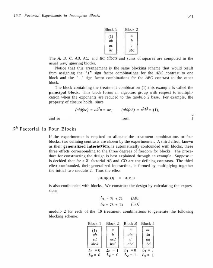
15.7 Factorial Experiments in Incomplete Blocks 641
Block 1
(1) ab ac be
Block 2
a b c
abc
The A, B, C, AB, AC, and BC effects and sums of squares are computed in the usual way, ignoring blocks.
Notice that this arrangement is the same blocking scheme that would result from assigning the ' ;+" sign factor combinations for the ABC contrast to one block and the "—" sign factor combinations for the ABC contrast to the other block.
The block containing the treatment combination (1) this example is called the principal block. This block forms an algebraic group with respect to multiplication when the exponents are reduced to the modulo 2 base. For example, the property of closure holds, since
(ab)(bc) = ab2c = ac, (ab)(ab) = a2b2 = (1),
and so forth. J
2k Factorial in Four Blocks
If the experimenter is required to allocate the treatment combinations to four blocks, two defining contrasts are chosen by the experimenter. A third effect, known as their generalized interaction, is automatically confounded with blocks, these three effects corresponding to the three degrees of freedom for blocks. The procedure for constructing the design is best explained through an example. Suppose it is decided that for a 24 factorial AB and CD are the defining contrasts. The third effect confounded, their generalized interaction, is formed by multiplying together the initial two modulo 2. Thus the effect
(AB)(CD) = ABCD
is also confounded with blocks. We construct the design by calculating the expressions
Lx = 71 + 72
E2 = 73 + 7i
(AB),
(CD)
modulo 2 for each of the 16 treatment combinations to generate the following blocking scheme:
Block 1
(1) ab cd
abed
Block 2
a b
acd bed
Block 3
c abc d
abd
Block 4
ac be ad bd
Lx = 0 L2 = 0
Li = l L2 = 0
Lx = 0 L2 = l
Li = l L2 = 1

642 Chapter 15 2k Factorial Experiments and Fractions
A shortcut procedure can be used to construct the remaining blocks after the principal block has been generated. Wc begin by placing any treatment combination not in the principal block in a second block and build the block by multiplying (modulo 2) by the treatment combinations in the principal block. In the preceding example the second, third, and fourth blocks are generated as follows:
Block 2
a(l) = a o.(ab) = b
a(cd) = acd a(abcd) = bed
Block 3
c(l) = ciab) = c(cd)
c(abcd)
- c abc
= d = abd
Block 4
ac(l) = ac(ab) = ac(cd) =
ac(abcd)
ac •-be ad
= bd
The analysis for the case of four blocks is quite simple. All effects that are orthogonal to blocks (those other than the defining contrasts) are computed in the usual fashion.
2k Factorial in 2P Blocks
The general scheme for the 2k factorial experiment in 2P blocks is not difficult. We select p defining contrasts such that none is the generalized interaction of any two in the group. Since there are 2P — 1 degrees of freedom for blocks, we have 2P - 1 — p additional effects confounded with blocks. For example, in a 26 factorial experiment in eight blocks, we might choose ACF, BCDE, and ABDF as the defining contrasts. Then
(ACF)(BCDE) = ABDEF,
(ACF)(ABDF) = BCD,
(BCDE)(ABDF) = ACEF,
(ACF)(BCDE)(ABDF) = E
are the additional four effects confounded with blocks. This is not a desirable blocking scheme, since one of the confounded effects is the main effect E. The design is constructed by evaluating
Lx = 7i + 73 + 76,
L2 = 72 + 73 + 74 + 75)
£3 = 7i + 7a + 74 + 76
and assigning treatment in combinations to blocks according to the following scheme:
Block 1: Lx = 0, L2= 0, L3 = 0
Block 2: L] = 0, L2= 0, L3 = 1
Block 3: L i = 0 , L2= 1, L3 = 0
Block 4: L i = 0 , L2= 1, L3 = 1
Block 5: Lx = 1, L2= 0, L3 = 0
Block 6: Lx = 1, L 2= 0, L3 = 1

15.7 Factorial Experiments in Incomplete Blocks 643
Block 7: Lx = 1, L2= 1, Lj, = 0
BlockS: £i = 1, L 2 = 1, L3 = 1.
The shortcut procedure that was illustrated for the case of four blocks also applies here. Hence we can construct the remaining seven blocks from the principal block.
Example 15.9:1 It is of interest to study the effect of five factors on some response with the assumption that interactions involving three, four, and five of the factors are negligible. We shall divide the 32 treatment combinations into four blocks using the defining contrasts BCDE and ABCD. Thus
(BCDE)(ABCD) = AE
is also confoundeel with blocks. The experimental design and the observations are given in Table 15.9.
Table 15.9: Data for a 25 Experiment in Four Blocks
Block 1
(1) = 30.6 tbc = 31.5 bd = 32.4 cd = 31.5
abe = 32.8 ace = 32.1 ade = 32.4
abcde = 31.8
Block 2
a = 32.4 abc = 32.4 abd = 32.1 acd = 35.3 be = 31.5 ce = 32.7 de = 33.4
bcde = 32.9
Block 3
/; = 32.6 c = 31.9 d = 33.3
bed = 33.0 ae = 32.0
abce = 33.1 abde = 32.9 acde = 35.0
Block 4
e = 30.7 bee = 31.7 bde = 32.2 cde = 31.8 ab = 32.0 ac = 33.1 ad = 32.2
abed = 32.3
The allocation of treatment combinations to experimental units within blocks is, of course, random. By pooling the unconfounded three-, four-, and five-factor interactions to form the error term, perform the analysis of variance for the data of Table 15.9.
Solution: The sums of squares for each of the 31 contrasts are computed and the block sum of squares is found to be
SS(blocks) = SS(ABCD) + SS(BCDE) + SS(AE) = 7.538.
The analysis of variance is given in Table 15.10. None of the two-factor interactions are significant at the a = 0.05 level when compared to /o.05(1-14) = 4.60. The main effects A and D are significant and both give positive effects on the response as we go from the low to the high level. _l
Partial Confounding It is possible to confound any effect with blocks by the methods described in Section 15.7. Suppose that we consider a 23 factorial experiment in two blocks with three complete replications. If ABC is confounded with blocks in all three replicates, we

644 Chapter 15 2k Factorial Experiments and Fractions
Table 15.10: Analysis of Variance for the Data of Table 15.9
Source of Variation Main effect:
A B C D E
Two-factor interaction: AB AC AD BC BD BE CD CE DE
Blocks (ABCD,
Error
BCDE,AE):
Sum of Squares
3.251 0.320 1.361 4.061 0.005
1.531 1.125 0.320 1.201 1.711 0.020 0.045 0.001 0.001 7.538
7.208
Degrees of Freedom
1 1 1 1 1
1 1 1 1 1 1 1 1 1 3
14
Mean Square
3.251 0.320 1.361 4.061 0.005
1.531 1.125 0.320 1.201 1.711 0.020 0.045 0.001 0.001 2.513
0.515
Computed /
6,32 0.62 2.64 7.89 0.01
2.97 2.18 0.62 2.33 3.32 0.04 0.09 0.002 0.002
can proceed as before and determine single-degree-of-freedom sums of squares for all main effects and two-factor interaction effects. The sum of squares for blocks has 5 degrees of freedom, leaving 23 — 5 — 6 = 12 degrees of freedom for error.
Now let us confound ABC in one replicate, AC in the second, and BC in the third. The plan for this type of experiment would be as follows:
Block Block Block 1 2 1 2 1 2
abc a b c
ab 0.C
be
(1)
abc ac b
(1)
ab be a c
abc be a
(1)
ab ac b c
Replicate 1 ABC Confounded
Replicate 2 AC Confounded
Replicate 3 BC Confounded
The effects ABC, AC, and BC are said to be partially confounded with blocks. These three effects can be estimated from two of the three replicates. The ratio 2/3 serves as a measure of the extent of the confounding. This ratio gives the amount of information available on the partially confounded effect relative to that available on an unconfounded effect.
The analysis-of-variance layout is given in Table 15.11. The sums of squares for blocks and for the unconfounded effects A, B, C, and AB are found in the usual way. The sums of squares for AC, BC, and ABC are computed from the two replicates in which the particular effect is not confounded. Wc must be careful

Exercises 645
to elivide by 16 instead of 24 when obtaining the sums of squares for the partially confounded effects, since we are only using 16 observations. In Table 15.11 the primes are inserted with the degrees of freedom as a reminder tha t these effects are partially confounded and require special calculations.
Table 15.11: Analysis of Variance with Part ia l Confounding
Source o f Var iat ion D e g r e e s o f F r e e d o m
B l o c k s
A B
C AB
AC
BC
ABC Error
Total
1 1 1 1 1' 1' l' 11
23
Exercises
15.13 In a 2'1 factorial experiment with 3 replications, show the block arrangement and indicate by means of tin analysis-of-variance table the effects to be tested and their degrees of freedom, when the AB interaction is confounded with blocks.
15.14 The following experiment was rnn to study main effects and all interactions. Four factors are used at two levels each. The experiment is replicated and two blocks are necessary in each replication. The data are presented here.
(a) What effect is confounded with blocks in the first replication of the experiment? In the second replication?
(h) Conduct an appropriate analysis of variance showing tests on all main effects and interaction effects. Use a 0.05 level of significance.
Replicate 1 Replicate 2 Block 1
(1) = 17.1 d = 16.8
ab = 16.4 ac = 17.2 6c = 16.8
abd = 18.1 acd= 19.1 bed = 18.4
Block 2 a = 15.5 b = 14.8 c = 16.2
ad = 17.2 bd = 18.3 cd = 17.3
abc = 17.7 abed =19.2
Block 3 (1) = 18.7 ab = 18.6 ac = 18.5 ad = 18.7 be = 18.9 bd = 17.0 cd = 18.7
abed = 19.8
Block 4 a = 17.0 b= 17.1 c= 17.2 d = 17.6
abc = 17.5 abd = 18.3 acd= 18.4 bcd= 18.3
15.15 Divide the treatment combinations of a 24 factorial experiment into four blocks by confounding ABC and ABD. What additional effect is also confounded with blocks?
15.16 An experiment is conducted to determine the breaking strength of a certain alloy containing five metals, A, B, C, D, and E. Two different percentages of each metal are used in forming the 25 = 32 different alloys. Since only eight alloys can be tested on a given day, the experiment is conducted over a period of 4 days during which the ABDE and the AE effects were confounded with days. The experimental data are given here.
(a) Set. up the blocking scheme for the 4 days. (b) What additional effect is confounded with days? (c) Obtain the sums of squares for all main effects.
Treat. Comb.
0) a h ab c. ac.
Breaking Strength
21.4 32.5 28.1 25.7 34.2 34.0
Treat. Comb.
e ae be a.l>e ce ace
Breaking Strength
29.5 31.3 33.0 23.7 26.1 25.9

646 Chapter 15 2k Factorial Experiments and Fractions
Treat. Comb.
be abc d ad bd abd cd acd bed abed
Breaking Strength
23.5 24.7 32,6 29.0 30.1 27.3 22.0 35.8 26.8 36.4
Treat. Comb. bee abce de ade bde abdc cde acde bede abede
Break ing S t r eng th
35.2 30.4 28.5 36.2 24.7 29.0 31.3 34.7 26.8 23.7
15.17 By confounding ABC in two replicates and AB in the third, show the block arrangement and the analysis-of-variance table for a 2'' factorial experiment with three replicates. What is the relative information on the confounded effects?
15.18 The following coded data represent the strength of a certain type of bread-wrapper stock produced under 16 different conditions, the latter representing two levels of each of four process variables. An operator effect was introduced into the model, since it was necessary to obtain half the experimental runs under operator 1 and half under operator 2. It. was felt that operators do have an effect, on the quality of the product.
(a) Assuming that all interactions are negligible, make significance tests for the factors A, B, C, and D. Use a 0.05 level of significance.
(b) What interaction is confounded with operators?
Operator 1
(1) = 18.8 ab = 16.5 ac = 17.8 be = 17.3 d = 1 3 . 5
abd= 17.6 acd = 18.5 bed = 17.6
Operator 2
a= 14.7 6=15 .1 c = 14.7
afcc = 19.0 ad = 16.9 bd= 17.5 cd = 18.2
abed =20.1
15.19 Consider a 25 experiment where the experimental runs are on 4 different machines. Use the machines as blocks, and assume that all main effects and two-factor interactions may be important.
(a) Which runs would be made on each of the 4 machines?
(b) Which effects are confounded with blocks?
15.20 An experiment is revealed in Myers and Montgomery (2002) in which optimum conditions are sought storing bovine semen to obtain maximum survival. The variables are percent sodium citrate, percent glyc
erol, and equilibration time in hours. The response is percent survival of the motile spermatozoa. The natural levels arc found in the above reference. Below are the data with coded levels for the factorial portion of the design and the center runs.
xi, Percent x2 X3 Sodium Percent Equilibration % Citrate Glycerol Time Survival
-1 1
-1 1
-1 1
-1 1 0 0
- 1 - 1
1 1
- 1 - 1
1 1 0 0
0 / 40 19 40 54 41 21 43 63 61
(a) Fit a linear regression model to the data and determine which linear and interaction terms are significant. Assume that the :cti2a;3 interaction is negligible.
(b) Test for quadratic lack of fit and comment.
15.21 Oil producers are interested in high strength-nickel alloys that are strong and corrosion resistant. An experiment conducted in which yield strengths were compared for nickel alloy tensile specimens charged in sulfuric acid solution saturated with carbon disulfide. Two alloys were combined; a 75% nickel composition and a 30% nickel composition. The alloys were tested under two different charging times, 25 and 50 days. A 23 factorial was conducted with the following factors
% sulfuric acid 4%, 6%: (xi)
charging time 25 days, 50 days: (#2)
nickel composition 30%, 75%: (2:3)
A specimen was prepared for each of the eight conditions. Since the engineers were not certain of the nature of the model (i.e., whether or not quadratic terms would be needed), a third level (middle level) was incorporated and four center runs were employed using four specimens at 5% sulfuric acid, 37.5 days, and 52.5% nickel composition. The following are the yield strengths in kilograms per square inch.
Charging Time 25 Days 50 Days
Nickel Sulfuric Acid Comp.
Sulfuric Acid 4% 6% 4% 6%
75% 30%
52.5 50.2
56.5 50.8
47.9 47.4
47.2 41.7
The center runs give the following strengths:
51.6, 51.4, 52.4, 52.9

15.8 Fractional Factorial Experiments 647
1,1
• • • (0,0)
o
1, 11
<> - 1 , - 1
Xl
1 , - 1
Figure 15.14: Graph for Exercise: 15.23.
(a) Test to determine which main effects and interactions should be involved in the fitted model.
(b) Test for quadratic curvature. (c) If quadratic curvature is significant, how many
additional elesign points are needed to determine which quadratic terms should be included in the model?
15.22 Suppose a second replicate of the experiment in Exercise 15.19 e:e>tild be performed. (a) Would a second replication of the blocking scheme
of Exercise 15.19 be the best choice? (b) If the answer to part (a) is no, give the layout for
a better choice for the second replicate. (c) What concept did you use in your ele'sign selection?
15.23 Consider Figure 15.14, which represents a 2" factorial with 3 center runs. If quadratic curvature is significant what additional design points would you select that might allow the estimation of the terms a;?,arf? Explain.
15.8 Fractional Factorial Experiments
The 2k factorial experiment can become1 quite: demanding, in terms of the number of experimental units required, when k is large. One of the real advantages with this experimental plan is that it allows a degree of freedom for each interaction. However, in many experimental situations, it is known that certain interactions are negligible, and thus it would be a waste of experimental effort to use the complete factorial experiment. In fact, the experimenter may have an economic constraint that disallows taking observations at all of the 2 t reatment combinations. When fc is large, we can often make use of a f r a c t i o n a l f a c t o r i a l e x p e r i m e n t where perhaps one-half, one-fourth, or even one-eighth of the total factorial plan is actually carried out .
Construction of \ Fraction
The construction of the half-replicate design is identical to the allocation of the 2k factorial experiment into two blocks. We' begin by selecting a defining contrast tha t is to be completely sacrificed. We then construct the two blocks accordingly and choose either of them as the experimental plan.
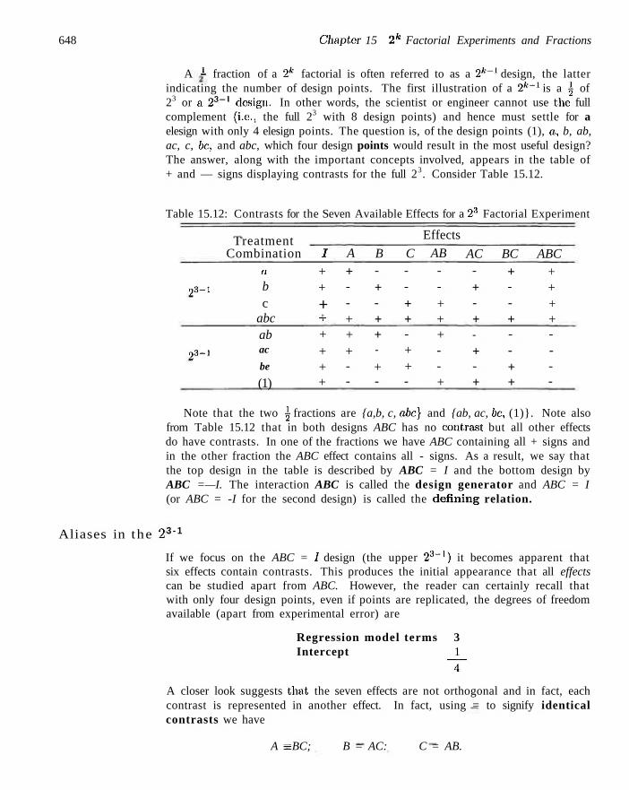
648 Chapter 15 2k Factorial Experiments and Fractions
A 1 fraction of a 2* factorial is often referred to as a 2k~l design, the latter indicating the number of design points. The first illustration of a 2k~l is a ^ of 23 or a 2 3 _ 1 design. In other words, the scientist or engineer cannot use the full complement (i.e.. the full 23 with 8 design points) and hence must settle for a elesign with only 4 elesign points. The question is, of the design points (1), a, b, ab, ac, c, be, and abc, which four design points would result in the most useful design? The answer, along with the important concepts involved, appears in the table of + and — signs displaying contrasts for the full 23. Consider Table 15.12.
Table 15.12: Contrasts for the Seven Available Effects for a 2:1 Factorial Experiment
23-1
2 3 - l
Treatment Combination
a
b c
abc ab ac
be
(1)
J
+ +
+ T
+ + + +
A
+ --+ + + --
B -+ -+ + -
+ -
C --+ + -+ + -
Effects
AB --+ + + --+
AC -+ -+ -
+ -+
BC + --+ --+ +
ABC + + + + ----
Aliases in the 2
Note that the two \ fractions are {a,b, c, abc} and {ab, ac, be, (1)}. Note also from Table 15.12 that in both designs ABC has no contrast but all other effects do have contrasts. In one of the fractions we have ABC containing all + signs and in the other fraction the ABC effect contains all - signs. As a result, we say that the top design in the table is described by ABC = I and the bottom design by ABC =—I. The interaction ABC is called the design generator and ABC = I (or ABC = -I for the second design) is called the denning relation.
3 - 1
If we focus on the ABC = / design (the upper 23_1) it becomes apparent that six effects contain contrasts. This produces the initial appearance that all effects can be studied apart from ABC. However, the reader can certainly recall that with only four design points, even if points are replicated, the degrees of freedom available (apart from experimental error) are
Regression model terms 3 Intercept 1
~4~
A closer look suggests that, the seven effects are not orthogonal and in fact, each contrast is represented in another effect. In fact, using = to signify identical contrasts we have
A s BC; B = AC: C = AB.

15.8 Fractional Factorial Experiments 649
As a result, within a pair an effect cannot be estimated independent of its alias "partner." In fact, the effects
o + abc — b — c and BC =
a + abc -b—c
will produce the same numerical result and thus contain the same information. In fact, it is often said that they share a degree of freedom. In truth, the estimated effect actually estimates the sum, namely A + BC. We say that A and BC are aliases, B and AC are aliases, and C and AB are aliases.
For the ABC = — I fraction we can observe that the aliases are the same as those for the ^4f?C = / fraction, apart from sign. Thus we have
A = -BC; B = -AC; C = -AB.
The two fractions appear on corners of the cube in Figure 15.15(a) and 15.15(b).
c
b a
S^abc
C
^ b c ac
ab/'
(a) The ABC = I fraction (b) The ABC = -I fraction
Figure 15.15: The \ fractions of the 23 factorial.
How Aliases Are Determined in General
In general, for a 2fc_1, each effect, apart from that defined by the generator, will have a single alias partner. The effect defined by the generator will not be aliased by another effect but rather is aliased with the mean since the least squares estimator will be the mean. To determine the alias for each effect, one merely begins with the defining relation, say ABC = / for the 2 3 _ 1 . Then to find, say, the alias for effect A, multiply .4 by both sides of the equation ABC = / and reduce any exponent by modulo 2. For example
A • ABC = A, thus BC = A.
In a similar fashion,
B = B • ABC = AB2C = AC,

650 Chapter 15 2k Factorial Experiments and Fractions
and. of course,
C = C- ABC = ABC2 = AB.
Now for the second fraction (i.e., defined by the relation ABC = —/),
A = -BC; B = -AC; C = -AB.
As a result, the numerical value of effect A is actually estimating A—BC. Similarly, the value of B estimates B — AC and the value for C estimates C — AB.
Formal Construction of the 2 k-l
A clear understanding of the concept of aliasing makes it very simple to understand the construction of the 2k_1. We begin with investigation of the 2 3 _ 1 . There are three factors and four design points required. The procedure begins with a full factorial in k - 1 = 2 factors A and B. Then a third factor is added according to the desired alias structures. For example, with ABC as the generator, clearly C = ± AB. Thus, C = AB or -AB is found to supplement the full factorial in A and B. Table 15.13 illustrates what is a very simple procedure.
Table 15.13: Construction of the Two 2 3 _ 1 Designs
Basic 22
A B
+ +
+ +
2:i
A
+ -+
-l.
B
—
+ j .
ABC C-
t I = AB
+
-+
2 3 - 1 ; . A B
+ -- + + +
ABC C =
= - J . : -AB
+ + -
Note that we saw earlier that ABC = I gives the design points a, b, c, and abc while ABC = —I gives (1), ac, be, and ab. Earlier we were able to construct the same designs using the table of contrasts in Table 15.12. However, as the design becomes more complicated with higher fractions, these contrast tables become more difficult to deal with.
Consider now a 2 4 - 1 (i.e., a ^ of a 24 factorial design) involving factors A, B, C, and D. As in the case of the 2 3 _ l , the highest-order interaction, in this case ABCD, is used as the generator. We must keep in mind that ABCD = / , the defining relation suggests that the information on ABCD is sacrificed. Here we begin with the full 23 in A, B, and C and form D = ± ABC to generate the two 2 4 _ 1 designs. Table 15.14 illustrates the construction of both designs.
Here, using the notations of a, b, c, and so on, we have the following designs:
ABCD = I, (1), ad, bd, ab, cd, ac, be, abed
ABCD = —/, d, a, b, abc, c, acd, bed, abc.
The aliases in the case of the 2'1_1 are found as illustrated earlier for the 2 3 _ 1 . Each effect has a single alias partner and is found by multiplication via the use of

15.8 Fractional Factorial Experiments 651
Table 15.14: Construction of the Two 2 4 _ 1 Designs
Basic 23
A B
+ -- + + + - -
+ -- + + +
C
— --
+ + + +
A
+ -+ -+ -
+
24-1.
B
—
+ + --
+ +
;ABCD
C
_ --
+ 4-
+ +
D =
= 1
= ABC
+ + -
+ --
+
A
+ -+ -+ -
+
2 4 - 1 ;
B
_
T
+ --+ +
ABCD =
C
— --j _
+ + +
D =
: -I
-ABC
+
-+ -+ + -
the defining relation. For example, the alias for .4 for the ABCD = / design is given by
A = A • ABCD = A2 BCD = BCD.
The alias for AB is given by
AB = AB • ABCD = A2B2CD = CD.
As we can observe easily, main effects are aliased with three factor interactions and two factor interactions are aliased with other two factor interactions. A complete listing is given by
A = BCD AB = CD
B = ACD AC = BD
C = ABD AD = BC
D = ABC.
Construction of the \ Fraction
In the case of the 4 fraction, two interactions are selected to be sacrificed rather than one, and the third results from finding the generalized interaction of the selected two. Note that this is very much like the construction of four blocks discussed in Section 15.7. The fraction used is simply one of the blocks. A simple example aids a great deal in seeing the connection to the construction of the 5 fraction. Consider the construction of \ of a 25 factorial (i.e., a 25~2), with factors A, B, C, D, and E. One procedure that avoids the confounding of two main effects is the choice of ABD and ACE as the interactions that correspond to the two generators, giving ABD = / and ACE = / as the defining relations. The third interaction sacrificed would then be (ABD)(ACE) = A2BCDE = BCDE. For the construction of the design, we begin with a 2 5 - 2 = 23 factorial in A, B, and C. We use the interactions ABD and ACE to supply the generators, so the 23 factorial in A, B, and C is supplemented by factor D = ± AB and E = ± AC.

652 Chapter 15 2k Factorial Experiments and Fractions
Thus one of the fractions is given by
A -
+ -
+ -+ -
+
B --
+ + --+ +
C ----
+ + + +
D = AB _i_
-—
+ + --
+
E = AC
+ -+ --
+ -+
de a be abd cd ace be abode
The other three fractions are found by using the generator {D = —AB, E = AC}, {D = AB.E = -AC}, and {D = -AB,E = -AC}. Consider an analysis of the above 25~2 design. It contains 8 design points to study five factors. The aliases for main effects are given by
A(ABD) = BD: A(ACE) = CE, A(BCDE) = ABCDE
B = AD = ABCE = CDE
C = ABCD =AE = BDE
D = AB = ACDE = BCE
E = ABDE =AC = BCD
Aliases for other effects can be found in the same fashion. The breakdown of degrees of freedom is given by (apart from replication)
Main effects Lack of fit Total
5 _2_ 7
(CD = BE, BC = DE)
We list interactions only through degree two in the lack of fit.
Consider now the case of a 2 6 - 2 , which allows 16 elesign points to study six factors. Once again two design generators are chosen. A pragmatic choice to supplement a 2G _ 2 = 24 full factorial in A, B, C, and D is to use E = ± ABC and F = ±BCD. The construction is given in Table 15.15.
Obviously, with 8 more design points than the 2 5 - 2 , the aliases for main effects will not present as difficult a problem. In fact, note that with defining relations ABCE = ± I, BCDF = ±1, and (ABCE)(BCDF) = ADEF = ± I, main effects will be aliased with interactions that are no less complex than those of third order. The alias structure for main effects is written
A= BCE = ABCDF = DEF,
B= ACE = CDF = ABDEF,
C= ABE = BDF = ACDEF.
D = ABCDE = BCF = AEF,
E = ABC = BCDEF = ADF,
F = ABCEF = BCD = ADE.

15.9 Analysis of Fractional Factorial Experiments 653
Table 15.15: A 2l'~2 Design
A — + -+ -+ -+ -+ -+ -+ -+
B — -+ + --+ + --+ + --+ +
C — ---+ + + + ----+ + + +
D — -------+ + + + + + j -
+
E = ABC — + + -+ --— -+ + -+ --+
F = BCD — -+ + + + --+ + ----+ +
Treatment Combination
(1) ae bef abf cef acf be abce df adef bde abd cde acd. bcdf abcdef
each with a single degree of freedom. For the two-factor interactions,
AB= CE - ACDF = BDEF, AF = BCEF = ABCD = DE,
AC= BE s ABDF = CDEF, BD = ACDE = CF = ABEF,
AD= BCDE = ABCF = EF, BF = ACEF = CD = ABDE,
AE= BC = ABCDEF = DF.
Here, of course, there is some aliasing among the two-factor interactions. The remaining 2 degrees of freedom are accounted for by the following groups:
ABD = CDE = ACF = BEF, ACD = BDE = ABF = CEF.
It becomes evident that we should always be aware of what the alias structure is for a fractional experiment before we finally recommend the experimental plan. Proper choice of defining contrasts is important, since it dictates the alias structure.
15.9 Analysis of Fractional Factorial Experiments
The difficulty of making formal significance tests using data from fractional factorial experiments lies in the determination of the proper error term. Unless there are data available from prior experiments, the error must come from a pooling of contrasts representing effects that are presumed to be negligible.
Sums of squares for individual effects are found by using essentially the same procedures given for the complete factorial. We can form a contrast in the treatment combinations by constructing the table of positive and negative signs. For

654 Chapter 15 2k Factorial Experiments and Fractions
example, for a half-replicate of a 23 factorial experiment with ABC the defining contrast, one possible set of treatment combinations, the appropriate algebraic sign for each contrast used in computing effects and the sums of squares for the various effects are presented in Table 15.16.
Table 15.16: Signs for Contrasts in a Half-Replicate of a 23 Factorial Experiment
Treatment Combination
Factorial Effect B AB AC BC ABC
a b c abc
+
+ +
+ +
+
+
+ + + +
Note that in Table 15.16 the A and BC contrasts are identical, illustrating the aliasing. Also, B — AC and C = AB. In this situation we have three orthogonal contrasts representing the 3 degrees of freedom available. If two observations are obtained for eae:h of the four treatment combinations, we would then have an estimate of the error variance with 4 degrees of freedom. Assuming the interaction effects to be negligible, we could test all the main effects for significance.
An example effect and corresponding sum of squares is
A = •b — c + abc
SSA = (a — b — c + abc)2
2n ' 22n In general, the single-degree-of-freedom sum of squares for any effect in a 2~v
fraction of a 2k factorial experiment (p < A:) is obtained by squaring contrasts in the treatment totals selected and dividing by 2k~''n, where n is the number of replications of these treatment combinations.
Example 15.10:1 Suppose that we wish to use a half-replicate to study the effects of five factors, each at two levels, on some response and it is known that whatever the effect of each factor, it will be constant for each level of the other factors. In other words, there are no interactions. Let. the defining contrast be ABCDE, causing main effects to be aliased with four factor interactions. The pooling of contrasts involving interactions provides 15 — 5 = 10 degrees of freedom for error. Perform an analysis of variance on the data in Table 15.17, testing all main effects for significance at the 0.05 level.
Solution: The sums of squares and effects for the main effects arc
SSA = (11.3 - 15.6 14.7 + 13.2)2 (-17.5)2
25-1 16 17.5
SSB
-2.19.
(-11.3 + 15.6 14.7 + 13.2)2 (18.1)2
0 5 - 1 16 B = ± | ! = 2.26,
SSC: (-11.3 - 15.6 + • • • + 14.7 4- 13.2)2 (10.3)2
2 5 - l 16
= 19.14,
= 20.48,
6.63,

15.9 Analysis of Fractional Factorial Experiments &bl
Table 15.17: Data for Example 15.10
Trea tmen t Response Trea tmen t Response
a b c d e abc abd acd
C7=3$a = 1.31,
?<T ( " U ' 3 ~
D = =$Z = -0.96.
5S(E) ( _ 1 L 3
•5.5 -Cj —
E = M = l .ll.
15.6
- 15.
11.3 15.6 12.7 10.1 9.2
11.0 8.9 9.6
bed abc ace adc bee bde ale abode
+ 14.7 + 13.2)2
25-1
6 2 5 - l
+ 14.r • + 13.2)2
14.1 14.2 11.7 9.4
16.2 13.9 14.7 13.2
<-f=,n
- • 7 —
All other calculations and tests of significance are summarized in Table 15.18. The tests indicate that factor A has a significant, negative effect on the response, whereas factor B lias a significant, positive effect. Factors C, D, and E are not significant at the 0.05 level. J
Table 15.18: Analysis of Variance for the Data of a Half-Replicate of a 25 Factorial Experiment
Source of Variat ion
Main effect A B C D E
Error Total
Sum of Squares
19.14 20.48
6.63 3.71 4.95
30.83 85.74
Degrees of Freedom
1 1 1 1 1
10 15
M e a n Square
19.14 20.48
6.63 3.71 4.95 3.0S
C o m p u t e d /
6.21 6.65 2.15 1.20 1.61

656
Exercises
Chapter 15 2k Factorial Experiments and Fractions
15.24 List the aliases for the: various effects in a 2 factorial experiment when the defining contrast is ACDE.
15.25 (a) Obtain a i fraction of a 21 factorial design using BCD as the defining contrast.
(b) Divide the \ fraction into 2 blocks of A units each by confounding ABC.
(c) Show the analysis-of-variance tabic (sources of variation and degrees of freedom) for testing all unconfounded main effects, assuming that all interaction effects are negligible.
15.26 Construct a \ fraction e>[ a 2° factorial elesign using ABCD and BDEF as the defining contrasts. Show what effects are: aliased with the six main effects.
15.27 (a) Using the defining contrasts ABCE and ABDF, obtain a j fraction of a 2° elesign.
(b) Show the analysis-of-variance! table (sources of variation and degrees of freedom) for all appropriate tests assuming that E and F do not interact and all three-factor and higher interactions are negligible.
15.28 Seven factors are' varied at, two levels in an experiment involving only 16 trials. A ;j fraction of a 2 factorial experiment is used with the defining contrasts being ACD, BEF, and CEG. The data are as follows:
Treat. C o m b .
(1 Ml abce cdef acef bade abdf hi
Response
31.6 28.7 33.1 33.6 33.7 34.2 32.5 27.8
Trea t . C o m b .
acg edg beg adefg efg abdeg bedfg abefg
Response 31.1 32.0 32.8 35.3 32.4 35.3 35.6 35.1
Perforin an analysis of variance em all seven main effects, assuming that interactions are negligible. Use a 0.05 level of significance.
15.29 An experiment is conducted sei that, an engineer can gain insight into the influence of sealing temperature A, cooling bar temperature B, percent polyethylene additive C, and pressure D on the seal strength (in grams per inch) of a. bread-wrapper Stock. A I fraction of a 2' factorial experiment is uscel with the defining contrast being ABCD. The data are: presented here. Perform an analysis of variance on main
effects, and two-factor interactions, assuming that all three-factor and higher interactions are negligible. Use a = 0.05.
A B C D Response
— 1
1 - 1
- 1 1
- I 1
- 1
- I 1
- 1 -1 1 1
- 1 1 1
- 1 1
- 1 - 1
1
6.6 6.9 7.9 (i.l 9.2 6.8
10.4 7.3 I
15.30 In an experiment conducted at the Department of Mechanical Engineering and analyzed by the Statistics Consulting Center at the Virginia Polytechnic Institute and State University, a sensor detects an electrical charge each time a turbine blade makes one; rotation. The sensor then measures the amplitude of the electrical current. Six factors arc rprn A, temperature B, gap between blades C, gap between blade and casing D, location of input E, and location of detection /•'. A j fraction of a 2° factorial experiment is used, with defining contrasts being ABCE and BCDF. The data are1 as follows:
A B - 1 - 1
1 - 1 - 1 1
1 1 - 1 - 1
1 - 1 - 1 1
1 1 - 1 - 1
1 - 1 - 1 L
1 1 - 1 - 1
1 - 1 - 1 1
I 1
C D - 1 - 1 - 1 - i - 1 - 1 - 1 - 1
1 - 1 1 - 1 1 - 1 1 - 1
- 1 1 - 1 1 - I 1
1 1 1 1 1 1 1 1 1 1
E - 1
1 1
- 1 1
- 1 - 1
1 - 1
1 1
- 1 1
- I - 1
1
F - 1 - 1
1 1 1 1 1
- 1 1 1
- 1 - 1 - 1 - 1
1 1
Response 3.89
10.46 25.98 39.88 61.88 3.22 8.94
20.29 32.07 50.76
2.80 8.15
16.80 25.47 44.44
2.45
Perform an analysis of variance on main effects, and two-factor interactions, assuming that all three-factor and higher interactions are negligible. Use a = 0.05.
15.31 In a study Durability of Rubber to Steel Adhesively Bonded Joints conducted at. the Department, of Environmental Science and Mechanics and analyzed by the Statistics Consulting Center at the Virginia Polytechnic Institute: and Stale University, an experimenter measures the number of breakdowns in an adhesive

15.10 Higher Fractions and Screening Designs 657
seal. It was postulated that concentration of seawafer A, temperature B, pH C, voltage D, and stress E influence the breakdown of an adhesive seal. A ^ fraction of a 2" factorial experiment is used, with the defining contrast being ABCDE. The data are as follows:
A - 1
1 - 1
1 - ]
1 - 1
1 - 1
1 - 1
1 - 1
1 -1
1
B -1 - 1
1 1
- 1 1 1 1
- 1 - 1
1 1
- 1 - 1
1 1
C - I
1 - 1 - 1
1 1 1 I
- 1 - 1 - 1 - 1
1 1 1 1
D 1
- 1 - 1 - 1 - I - 1 - 1 - 1
1 1 1 1 1 1 I 1
E
I - 1 - 1
1 - 1
1 1
- 1 - 1
1 1
- 1 1
- 1 - 1
1
Response 462 746 714
1070 474 832 764
1087 522 854 773
1068 572 831 819
1101
Perform an analysis of variance on main effects, and two-factor interactions, assuming that all three-factor and higher interactions are negligible. Use ev = 0.05.
15.32 Consider a 2r>_1 elesign with factors A, B, C, D, and E. Construct the design by beginning with a 2'1 and use E = ABCD as the generator. Show all aliases.
15.33 There arc six factors and only 8 elesign points can be used. Construct 23 and use D = AB, E
a 2 by beginning with a
generators.
15.34 Consider Exercise 15.33. Construct another 2''~'! that is different from the design chosen in Exercise 15.33.
15.35 for Exercise 15.33, give all aliases for the six main effects.
15.36 In Myers and Montgomery (2002), an application was discussed in which an engineer is concerned with the effects on the cracking of a fit antum alloy. The three factors are A, temperature, B, titanium content, and C, amount of grain refiner. The following gives a portion of the design and the response, crack length induced in the sample of the alloy.
A B C Response
I
I 0.5269 2.3380 4.0060 3.3640
AC and F = BC the
(a) What is the defining relation?
(b) Give aliases for all three main effects assuming that two factor interactions may be real,
(c) Assuming that interactions are' negligible, which main Factor is most important?
(d) For the factor named in (c), at. what level would you suggest, the factor be for final production, high or low?
(c) At what levels would you sugge:st the other factors be for final production?
(f) What hazards lie in the recommendations you made' in (d) and (e)? Be thorough in your answer.
15.10 Higher Fractions and Screening Designs
Some industrial situations require the analyst to determine which of a large number of controllable factors have an impact on some impor tant response. The factors may be qualitative eir class variables, regression variables, or a mixture of both . The analytical procedure may involve analysis of variance, regression, or both. Often the regression model used involves only linear main effects, although a fewr
interactions may be estimated. The situation calls for variable: screening and the resulting experimental designs are known as s c r e e n i n g d e s i g n s . Clearly, two-level orthogonal efosigns that are sa turated or nearly sa tura ted are viable candidates.
Design Resolution
Two-level orthogonal designs are often classified according to their r e s o l u t i o n , the latter determined through the following definition.

658 Chapter 15 2k Factorial Experiments and Fractions
Definition 15.1: The resolution of a two-level orthogonal elesign is the length of the smallest (least complex) interaction among the set of defining contrasts.
If the design is constructed as a full or fractional factorial [i.e., either a 2 or 2k~p (p = 1,2,..., A: - 1) design], the notion of design resolution is an aid in categorizing the impact of the aliasing. For example, a resolution II design would have little use since there would be at least one instance of aliasing of one main effee-t with another. A resolution III elesign will have all main effects (linear effects) orthogonal to each other. However, there will be some aliasing among linear effects and two-factor interactions. Clearly, then, if the analyst, is interested in studying main effects (linear effects in the case of regression) and there are no two-factor interactions, them a, elesign of resolution at least III is required.
15.11 Construction of Resolution III and IV Designs with 8, 16, and 32 Design Points
Useful designs of resolutions III and IV can be constructed for 2 to 7 variables with 8 design points. We merely begin with a 23 factorial that has been symbolically saturated with interactions.
Xl
- 1 1
-1 -1 1 1
-1 1
x2 - 1 -1 1
-1 1
-1 1 1
X3
-1 -1 -1 1
-1 1 1 1
xi-r2
1 -1 -1 1 1
-1 -1 1
X1X3 1
-1 1
-1 -1 1
-1 1
x2x3
1 1
-1 -1 -1 -1 1 1
XiX2
- 1 1 1 1
-1 - 1 -1 1
It is clear that a resolution III elesign can be constructed merely by replacing interaction columns by new main effects through 7 variables. For example, we may elefine
x4 = Xix2 (defining contrast ABD)
x-j = .('i.r.j (defining contrast ACE)
x$ = x2x3 (defining contrast BCF)
x- = 3:1X2X3 (defining contrast ABCG)
and obtain a 2 a fraction of a 2' factorial. The preceding expressions identify the chosen defining contrasts. Eleven additional defining contrasts result and all defining contrasts t:ontain at least three letters. Thus the design is a resolution III design. Clearly, if we begin with a. subset of the augmented columns and conclude with a design involving fewer than seven elesign variables, the result is a resolution III design in fewer than 7 variables.
A similar set of possible designs can be constructed for 16 elesign points by beginning with a 2'1 saturated with interactions. Definitions of variables that correspond to these interactions produce resolution III elesigns through 15 variables.

15.11 Construction of Resolution III and IV Designs 659
N u m b e r of Factors
3 4 5
6
Table 15.19: Some Resolution III. IV, and V 2k~v Designs
Design 2 3 - l '•III 2 , l - i 2 5 - 2 LIV 2 n- i r,(i-2 AVl 0 6- : i
Number of Points
4 8 8
32 16 8
Generators
C = ± AB D = ± ABC D = ± AB; E=± AC
F = ±BCD E = ± ABC; F = ±BCD D = ±AB; F = ±BC; E = ±AC
2 7 - l
07-2 LIV 27-. 'l
2 7 - l
64 32
16 8
G = ± ABCDEF E = ± ABC; G=± ABDE
E = ± ABC; F-± BCD; G = ± ACD D = ± AB; E = ±AC; F = ± BC; G = ± ABC
2 | r 2 64 G=± ABCD; H = ± ABEF 2°Z3 32 F = ± ABC; G = ± ABD; H = ± BCDE 2%* 16 E = ± BCD; F = ± ACD; G = ± ABC; H = ± ABD
In a similar fashion, designs containing 32 runs can be constructed by beginning with a 25.
Table 15.19 provides the user with guidelines for constructing 8. 16, 32, and 64 point designs that are resolution III, IV and even V. The table gives the number of factors, number of runs, and the generators that are used to produce the 2k~p
designs. The generator given is used to augment the full factorial containing k — p factors.
The Foldover Technique
We can supplement the resolution III designs described previously, to produce a resolution IV design by using a foldover technique. Foldover involves doubling the size of the design by adding the negative of the design matrix constructed as described above. Table 15.20 shows a 16-run resolution IV design in 7 variables constructed by using the foldover technique. Obviously, we can construct resolution IV designs involving up to 15 variables by using the foldover technique on designs developed by the saturated 24 design.
This design is constructed by "folding over" a 1 fraction of a 26. The last column is added as a seventh factor. In practice, the last column often plays the role of a blocking variable. The foldover technique is used often in sequential experimentation where the data from the initial resolution III design are analyzed. The experimenter may then feel, based on the analysis, that a resolution IV design is needed. As a result, a blocking variable may be needed because a separation in time occurs between the two portions of the experiment. Apart from the blocking variable, the final design is a 1 fraction of a 2e experiment.

660 Chapter 15 2k Factorial Experiments and Fractions
Table 15.20: Resolution IV Two-Level Design, Using the Foldover Technique
Xl
-L 1
-1 -1 1 1
-1 1
x-> -1 -1 1
-1 1
-1 1 1
X;i
-1 -1 -1 1
-1 1 1 1
X4 = Xi
1 -1 -1 1 1
-1 -1 1
x2 Xs = X1X3
1 -1 1
-1 -1 1
-1 1
X6 — X2X3
1 1
-1 -1 -1 -1 1 1
•''7
-I -1 -1 -1 -1 -1 -1 -1
Foldover
1 -1 1 1
-1 -1 1
-1
1 1
-1 1
-1 1
-1 -1
1 1 1
-1 1
-1 -1 -1
-1 1 1
-1 -1 1 1
-1
-1 1
-1 1 1
-1 1
-1
-1 -1 1 1 1 1
-1 -1
1 1 1 1 I 1 1 1
15.12 Other Two-Level Resolution III Designs; The Plackett-Burman Designs
A family of designs developed by Plackctt and Burman (see the Bibliography) fills sample size voids that exist with the fractional factorials. The latter arc useful with sample sizes 2 r (i.e., they involve' sample sizes 4,8,16,32,64,. . . ) . The Plackett-Burman designs involve 2r design points, and thus designs of size 12, 20, 24, 28, and so on are available. These two-level Plackett-Burman designs are resolution III designs and arc very simple to construct. "Basic lines*' arc given for each sample size. These lines of -I- and — signs are n — 1 in number. To construct the columns of the elesign matrix, we begin with the basic line and do a cyedic permutation on the columns until k (the elesired number of variables) columns are formed. Then, we fill in the last row with negative signs. The result will be a resolution III design with k variables (k = 1,2,..., A'). The basic lines are: as follows:
N= 12
N = 16
N = 20
N = 24
+ + + +
+ - + + + + T — —
+ + +
+ + - - - + - + - + + -+ + + + - + + - + - + +
+ + + + + + -
Example 15.11:1 Construct a two-level screening design with 6 variabilis containing 12 design points. Solution: Begin with the basic line in the initial column. The second column is formed by
bringing the bottom entry of the first column to the top of the seconel column

15.13 Robust Parameter Design 661
and repeating the first column. The third column is formed in the same fashion, using entries in the second column. When there is a sufficient number of columns, simply fill in the last row with negative signs. The resulting design is as follows:
Xl
+ --
+ + + ---+
x2 -+ + -+ + + --—
xa + -+ + -+ + + --
XA -+ -+ + -+ l-
+ —
x5 --+ -+ + -+ + +
X,
-— -+ — + + -+ +
1-
The Plackett-Burman designs arc popular in industry for screening situations. As resolution III designs, all linear effects are orthogonal. For any sample size, the user has available a design for k — 2 , 3 , . . . , Ar — 1 variables.
The alias structure for the Plackett-Burman design is very complicated and thus the user cannot construct the design with complete control over the alias structure as in the case of 2k or 2k~p designs. However, in the case of regression models the Plackett-Burman design can accommodate interactions (although they
will not be orthogonal) when sufficient, degrees of freedom are available. J
15.13 Robust Parameter Design
In this chapter we have emphasized the notion of using design of experiments (DOE) to learn about engineering and scientific processes. In the case where the process involves a product, DOE can be used to provide product improvement or quality improvement. As we: point out in Chapter 1, much importance has been attached to the use of statistical methods in product improvement. An important aspect of this quality improvement effort of the 1980s and 1990s is to design quality into processes and products at the research stage or the process design stage. One often requires DOE in the development of processes that have the following properties:
1. Insensitive (robust) to environmental conditions
2. Insensitive (robust) to factors difficult to control
3. Proviele minimum variation in performance
These methods are: often called robust parameter design (sec Taguchi, Taguchi and Wu, and Kackar in the Bibliography). The term design, in this context refers to the elesign of the process or system; parameter refers to the parameters in the system. These arc what we: have been calling factors or variables.

662 Chapter 15 2k Factorial Experiments and Fractious
It is very clear that, goals 1. 2. and 3 above are quite noble. For example, a petroleum engineer may have a fine gasoline blend that performs quite well as long as conditions are ideal and stable. However, the performance may deteriorate because of changes in environmental conditions, sue'h as type of driver, weather conditions, type of engine, and so forth. A scientist at a food company may have a cake mix that is quite good unless the user does not exactly follow directions on the box directions that deal with oven temperature, baking time, and so forth. A product or process whose performance is consistent when exposed to these changing environmental conditions is called a robust product or robust process. [See Myers and Montgomery (2002) in the Bibliography.]
Control and Noise Variables
Taguchi emphasized the notion of using two types of design variables in a study. These factors are control factors and noise1 factors.
Definition 15.2: Control factors are variables that can be controlled in both the experiment and in the process. Noise factors arc variables that may or may not be controlled in the experiment but cannot be controlled in the process (or not controlled well in the process).
An important approach is to use control variables and noise variables in the same experiment as fixed effects. Orthogonal designs or orthogonal arrays are popular designs to use in this effort.
Goal of Robust The goal of robust parameter efesign is to choose the levels of the control vari-Paraineter Design ables (i.e., the design e>f the process) that are most, robust (insensitive) to change's
in the noise variables.
It should be noted that changes in the noise variables actually imply changes during the process, changes in the field, changes in the environment, changes in handling or usage by the consumer, and so forth.
The Product Array-One approach to the elesign of experiments involving both control anel noise variables is the use of an experimental plan that calls for an orthogonal design for both the control and the noise variables separately. The: complete experiment, then, is merely the product or crossing of these two orthogonal designs. The following is a simple example of a product array with two control and two noise variables.
Example 15.12:1 In the article ''The Taguchi Approach to Parameter Design'' by D. M. Byrne and S. Taguchi, in Quality Progress. December 1987, the authors discuss an interesting example in which a method is sought to assemble an ele:ctrometi'ic connector to a nylon tube that delivers the required pull-off performance to be suitable for an automotive engine application. The objective is to find controllable conditions that maximize pull-off force Among the controllable variables are A, connector wall thickness, and B, insertion elepth. During routine operation there are several variables that cannot be controlled, although they will be controlled during

15.13 Robust Parameter Design 663
Analysis
the experiment. Among them are C, conditioning time, and D, conditioning temperature. Three levels are taken for each control variable and two for each noise variable'. As a result, the crossed array is as follows. The control array is a 3 x 3 array and the noise array is a familiar 22 factorial with (1), c, d, and cd representing the factor combinations. The purpose of the noise factor is to create the kind of variability in the response, pull-off force, that might be expected in day-to-day operation with the process. The design is shown in Table 15.21. J
Table 15.21: Design for Example 15.12
B (depth) Shallow Medium Deep
Thin
Medium
(D c
d cd
(1) c
d cd
(1) c
d cd
(1) c
d cd
(1) c
d cd
(1) c
d cd
Thick
(1) c
d cd
(1) (1) c c
d d cd cd
There are several procedures for analysis of the product array. The approach advocated by Taguchi and adopted by many companies in the United States dealing in manufacturing processes involves, initially, the formation of summary statistics at each combination in the control array. This summary statistic is called a signal-to-noise ratio. Suppose that we call yi,y>, • • • ,y„ a typical set of experimental runs for the noise array at a fixed control array combination. Table 15.22 describes some of the typical SN ratios.
Table 15.22: Typical SN Ratios under Different Objectives
Objective SN Ratio
Maximize response SNr, = —10 log ( ^ £
Achieve target SNT
Minimize response SN„
10 log < ( * )
io fog £ £ w t = l

664 Chapter 15 2k Factorial Experiments and Fractions
For each of the cases above we seek to find the combination of the control variables that maximizes SN.
Example 15.13:1 Case Study In an experiment described in Understanding Industrial Designed Experiments by Schmidt and Launsby (see the Bibliography), solder process optimization is accomplished by a printed circuit-board assembly plant. Parts are inserted either manually or automatically into a bare board with a circuit printed on it. After the parts are inserted the board is put through a wave solder machine, which is used to connect all the parts into the circuit. Boards are placed on a conveyor and taken through a series of steps. They are bathed in a flux mixture to remove oxide. To minimize warpage, they are preheated before the solder is applied. Soldering takes place as the boards move across the wave of solder. The object of the experiment is to minimize the number of solder defects per million joints. The control factor and levels are as given in Table 15.23.
Table 15.23: Control Factors for Example 15.13
Factor A, solder pot temperature (°F) B, conveyor speed (ft/min) C, flux density D, preheat temperature E, wave height (in.)
( -1) 480 7.2 0.9° 150 0.5
(+1) 510 10 1.0° 200 0.6
These factors are easy to control at the experimental level but are more formidable
at the plant or process level. J
Noise Factors: Tolerances on Control Factors Often in processes such as this one the natural noise factors are tolerances in the control factors. For example, in the actual on-line process, solder pot temperature and conveyor speed are difficult to control. It is known that the control of temperature is within ±5°F and the control of conveyor belt speed is within ±0.2 ft/min. It is certainly conceivable that variability in the product response (soldering performance) is increased because of an inability to control these two factors at some nominal levels. The third noise factor is the type of assembly involved. In practice, one of two types of assemblies will be used. Thus we have the noise factors given in Table 15.24.
Both the control array (inner array) and the noise array (outer array) were chosen to be fractional factorials, the former a | of a 25 and the latter a ^ of a 23, The crossed array and the response values are shown in Table 15.25. The first three columns of the inner array represent a 23. The columns are formed by D = —AC and E = —BC. Thus the defining interactions for the inner array are ACD, BCE, and ADE. The outer array is a standard resolution III fraction of a 23. Notice that each inner array point contains runs from the outer array. Thus four response values are observed at each combination of the control array. Figure 15.16 displays plots which reveal the effect of temperature and density on the mean response.

15.13 Robust. Parameter Design G65
Table 15.24: Noise Factors for Example 15.13
Factor ( -1) (+1) A*, solder pot temperature tolerance (°F)
(deviation from nominal) B*, conveyor sliced tolerance (ft/min)
(deviation from ideal) C*, assembly type
-5°
0.2
1
-5°
+0.2
2
Table: 15.25: Cross Arrays and Response Values for Example 15.13
Inner Array Ou te r Array A 1 1 1 J
-1 -1 -1 -1
B 1 1
-1 -1 1 1
-1 -1
C I
-1 1
-I 1
-1 1
-1
D -1 I
-1 1 1
-1 1
-1
E -1 1 1
-1 -1 1 1
-1
(1) 194 136 185 47 295 234 328 186
a*b* 197 136 261 125 216 159 326 187
a*c* 193 132 264 127 204 231 247 105
b*c* 275 136 264 42 293 157 322 104
SNS
-46.75
-42.61 -47.81
-39.51
-48.15
-45.97
-45.76
-43.59
Temperature and flux density are the most important factors. They seem to influence both (SN)s and y. Fortunately, high temperature and low flux: density arc preferable for both (SN)s- anel the mean response. Thus the "optimum" conditions are
solder temperature = 510°F, 11 ux density =0.9° .
250
>
120
Temperature
Low (-D
High (+D
250
I 185
120
Density
Low (-1)
High (+1)
Figure 15.16: Plot showing the influence of factors on the: mean response.

666 Chapter 15 2k Factorial Experiments and Fractions
Alternative Approaches to Robust Parameter Design
One approach suggested by many is to model the sample mean anel sample variance separately rather than combine the two separate concepts via a signal-to-noise ratio. Separate modeling often helps the experimenter to obtain a better understanding of the process involved. In the following example, wc illustrate this approach with the solder process experiment.
Example 15.14: Consider the data set of Example 15.13. An alternative analysis is to fit separate models for the mean y and the sample standard deviation. Suppose that we use the usual +1 and —1 coding for the control factors. Based on the apparent importance of solder pot temperature a?i and flux density x2, linear regression model on the response (number of errors per million joints) produces the model
y = 197.125 - 27.5a:i + 57.875.i.-2.
To find the most robust level of temperature and flux density it is important to procure a compromise between the mean response anel variability, which requires a modeling of the variability. An important tool in this regard is the log transformation (see Bartlett anel Kendall or Carroll and Ruppert):
In S3 = 7o + 71 (xi) + J2ix2).
This modeling process produces the following result:
I n > 6.7692 - 0.8178.7:, 4- 0.6877x2.
The analysis that is important, to the scientist or engineer is to make use of the two models simultaneously. A graphical approach can be very useful. Figure 15.17 shows simple plots of the mean and standard deviation simultaneously. As one would expect, the: location in temperature and flux density that minimizes the mean number of errors is the same as that which minimizes variability, namely-high temperature and low flux density. The graphical multiple response approach allows the: user to see tradeoffs between process mean and process variability. Feir this example, the engineer may be dissatisfied with the extreme conditions in solder temperature and flux density. The figure offers estimation of mean and variability conditions that indicate how much is lost as erne moves away from the optimum to any intermediate conditions. J
Exercises
15.37 Use: the coal cleansing data of Exercise page 622 to fit a model of the type
E(Y) = 0Q + ftjpi -t- 02X7 + P3X3,
where the levels arc
:z'i: percent solids: 8; 12 :ro: flow rate: 150: 250 gal/min :K3: pll: 5; 6
Center and scale the variables to design units. Also conduct a test for lack of fit, and comment concerning the adequacy e>f the linear regression model.

Review Exercises 667
in
a> Q
_3
-0.5
0.0
X), Temperature
1.0
Figure 15.17: Mean and s tandard deviation for Example 15.14.
15.38 A 2° factorial plan is used to build a regression model containing first-order coefficients and model terms for all two-factor interactions. Duplicate runs are made for each factor. Outline the analysis-of-variance table showing degrees of freedom for regression, lack of fit, and pure error.
Consider the -^ of the 27 factorial discussed in 15.39 Section 15.11. List the additional 11 defining contrasts.
15.40 Construct a Plackett-Burman design for 10 variables containing 24 experimental runs.
Review Exercises
15.41 A Plackett-Burman design is used for the purpose of studying the rheological properties of high-molecular-weight, copolymers. Two levels of each of six variables are fixed in the experiment. The viscosity of the polymer is the respemse. The data were analyzed by the Statistics Consulting Center at Virginia Polytechnic Institute and State University for personnel in the Chemical Engineering Department at the University. The variables are as follows: hard block chemistry xi, nitrogen flow rate X2, heat-up time x-z, percent compression x4, scans high and low £5, percent strain XQ. The data are presented here. Build a regression equation relating viscosity to the levels of the six variables. Conduct f-tests for all main effects. Recommend factors that should be retained for future studies and those that should not. Use the residual mean square (5 degrees of freedom) as a measure of experimental error.
Obs. x% X2 Xa x4 Xs Xe 1 1 - 1 1 2 1 1 - ' 3 - 1 1 ' 4 1 - 1 : 5 1 1 - : 6 1 1 1 7 - 1 1 1 8 - 1 - 1 : 9 - 1 - 1 -
10 1 - 1 -1 1 - 1 1 -12 - 1 - 1 -
1 - 1 - 1 - 1 I 1 - 1 - 1 I - 1 1 - 1 1 1 - 1 1 1 1 1 - 1 1 - 1 1 1 1 1 - 1 1 I 1 1 - 1 1 1 1 1 I - 1 1 1 1 - 1 - 1 1 1 - 1 - 1 - 1
194,700 588,400
7,533 514,100 277.300 493,500
8,969 18,340 6,793
160,400 7,008 3,637
15.42 A large petroleum company in the Southwest regularly conducts experiments to test additivess to drilling fluids. Plastic viscosity is a rheological measure reflecting the thickness of the fluid. Various polymers are added to the fluid to increase viscosity. The following is a data set in which two polymers are used at

668 Chapter 15 2k Factorial Experiments and Fractions
two levels each and the viscosity measured. The concentration of the polymers is indicated as "low" and "high." Conduct an analysis of the 22 factorial experiment. Test for effects for the two polymers and interaction.
Polymer 2 Low High
Polymer 1 Low High
3 3.5 11.7 12.0
11.3 12.0 21.7 22.4
15.43 A 22 factorial experiment is analyzed by the Statistics Consulting Center at Virginia Polytechnic Institute and State University. The client is a member of the Department of Housing, Interior Design, and Resource Management. The client is interested in comparing cold start versus preheating ovens in terms of total energy being delivered to the product. In addition, the conditions of convection are being compared to regular mode. Four experimental runs were made at each of the four factor combinations. Following are the data from the experiment:
Convection Mode Regular Mode
Preheat 618 619.3 629 611 581 585.7 581 595
Cold 575 573.7 574 572 558 562 562 566
Do an analysis of variance to study main effects and interaction. Draw conclusions.
15.44 Construct a design involving 12 runs where 2 factors are varied at 2 levels each. You are further restricted in that blocks of size 2 must be used, and you must be able to make significance tests on both main effects and the interaction effect.
15.45 In the study The Use of Regression Analysis for Correcting Matrix Effects in the X-Ray Fluorescence Analysis of Pyrotechnic Compositions, published in the Proceedings of the Tenth Conference on the Design of Experiments in Army Research Development and Testing, ARO-D Report 65-3 (1965), an experiment was conducted in which the concentrations of 4 components of a propellant mixture and the weights of fine and coarse particles in the slurry were each allowed to vary. Factors .4, B, C, and D, each at two levels, represent the concentrations of the 4 components and factors E and F, also at two levels, represent the weights of the fine and coarse particles present in the slurry. The goal of the analysis was to determine if the X-ray intensity ratios associated with component 1 of the propellant were significantly influenced by varying the concentrations of the various components and
the weights of the particle sizes in the mixture. A | fraction of a 26 factorial experiment was used with the defining contrasts being ADE, BCE, and ACF. The following data represent the total of a pair of intensity readings:
Treatment Intensity Batch Combination Ratio Total
1 2 3 4 5 6 7 8
abef cdef (1) ace bde abed adf bef
2.2480 1.8570 2.2428 2.3270 1.8830 1.8078 2.1424 1.9122
The pooled mean square error with 8 degrees of freedom is given by 0.02005. Analyze the data using a 0.05 level of significance to determine if the concentrations of the components and the weights of the fine and coarse particles present in the slurry have a significant influence on the intensity ratios associated with component 1. Assume that no interaction exists among the 6 factors.
15.46 Show the blocking scheme for a 27 factorial experiment in eight blocks of size 16 each, using ABCD, CDEFG, and BDF as defining contrasts. Indicate which interactions are completely sacrificed in the experiment.
15.47 Use Table 15.19 to construct a 16-run design with 8 factors that is resolution IV.
15.48 In your design of Review Exercise 15.47, verify that the design is indeed resolution IV.
15.49 Construct a design that contains nine design points, is orthogonal, contains 12 total runs, 3 degrees of freedom for replication error, and allows for a lack of fit test for pure quadratic curvature.
15.50 Consider a design which is a 23rj/ w4th 2 cen
ter runs. Consider y/ as the average response at the design parameter and j/o as the average response at the design center. Suppose the true regression model is
E(y) = 00+ 0lXl + 02X2 + 03x3
+ 0lix\ + 022X1+033X1.
(a) Give (and verify) E(yj — y0). (b) Explain what you have learned from the result in
(a).

15.14 Potential Misconceptions and Hazards; Relationship to Material in Other Chapters 669
15.14 Potential Misconceptions and Hazards; Relationship to Material in Other Chapters
In the use of fractional factorial experiments one: eif the most, important considerations that the analyst must be aware of is the design, resolution. A design of low resolution is smaller (and hence cheaper) than one of higher resolution. However, a price is paid for the cheaper design. The: elesign of lower resolution has heavier aliasing than one' of higher resolution. For example, if the researcher has expectation that two-factor interactions may be important, then resolution III should not be used. A resolution III elesign is strictly a main effects plan.

Chapter 16
Nonparametric Statistics
16.1 Nonparametric Tests
Most of the hypothesis-testing procedures discussed in previous chapters are based on the assumption that the random samples are selected from normal populations. Fortunately, most of these tests are still reliable when we expedience slight elepar-tures from normality, particularly when the sample size is large. Traditionally, these testing procedures have been referred to as pa ramet r i c me thods . In this chapter we consider a number of alternative test procedures, called nonparamet ric or distr ibution-free methods , that often assume no knowledge whatsoever about the distributions of the underlying populatiems, except perhaps that they are continuous.
Nonparametric or distribution-free procedures are used with increasing frequency by data, analysts. There: are many applications in science and engineering where the data are reported as values not on a continuum but rather on an ordinal scale such that it is quite natural to assign ranks to the data. In fact, the reader may notice quite early in this chapter that the distribution-free methods described here involve an analysis of ranks. Most analysts find the computations involved in nonparametric methods to be very appealing and intuitive.
For an example where a. nonparametric test is applicable, two judges might rank five brands of premium beer by assigning a rank of 1 to the brand believed to have the best overall quality, a rank of 2 to the second best, and so forth. A nonparametric te:st could then be used to determine whether there is any agreement be-tween the two judges.
We shoulel also point out that there are a number of disadvantages associated with nonparametric tests. Primarily, they do not utilize all the information provided by the sample, anel thus a nonparametric test will be less efficient than the corresponeUng parametric procedure when both methods are applicable. Consequently, to achieve the same power, a nonparametric test will require a larger sample size than will the corrcsponeliiig parametric test.
As we indicated earlier, slight departures from normality result in minor deviations from the ideal for the standard parametric tests. This is particularly true for the /-test and the F-test. In the case of the t-test and the F-test. the P-value

672 Chapter 16 Nonparametric Statistics
quoted may be slightly in error if there is a moderate violation of the normality assumption.
In summary, if a parametric and a nonparametric test are both applicable to the same set of data, we should carry out the more efficient parametric technique. However, we should recognize that, the assumptions of normality often cannot be justified and that we do not always have quantitative measurements. It is fortunate that statisticians have provided us with a number of useful nonparametric procedures. Armed with nonparametric techniques, the data analyst has more ammunition to accommodate a wider variety of experimental situations. It should be pointed out that even under the standard normal theory assumptions, the efficiencies of the nonparametric techniques are remarkably close to those of the corresponding parametric procedure. On the other hand, serious departures from normality will render the nonparametric method much more efficient than the parametric procedure.
Sign Test
The reader should recall that the procetiures discussed in Section 10.7 for testing the null hypothesis that p = po arc valid only if the population is approximately normal or if the sample is large. However, if n < 30 and the population is decidedly nonnormal, we must resort to a nonparametric test.
The sign test is used to test hypotheses on a population median. In the case of many of the nonparametric procedures, the mean is replaced by the median as the pertinent location paramete r under test. Recall that the sample median is defined in Section 1.4. The population counterpart, denoted by p has an analogous definition. Given a random variable X, p. is defined such that P(X > p.) < 0.5 and P(X < p) < 0.5. In the continuous case,
P(X > ft) = P(X < A) = 0.5.
Of course, if the distribution is symmetric, the population mean and median are equal. In testing the null hypothesis H0 that p — po against an appropriate alternative, on the basis of a random sample of size n, we replace each sample value exceeding po with a plus sign and each sample value less than po with a minus sign. If the null hypothesis is true and the population is symmetric, the sum of the plus signs should be approximately equal to the sum of the minus signs. When one sign appears more frequently than it should, based on chance alone, we reject the hypothesis that the population median p is equal to p0.
In theory the sign test is applicable only in situations where po cannot equal the value of any of the observations. Although there is a zero probability of obtaining a sample observation exactly equal to po when the population is continuous, nevertheless, in practice a sample value equal to po will often occur from a lack of precision in recording the data. When sample values equal to po are observed, they are excluded from the analysis and the sample size is correspondingly reduced.
The appropriate test statistic for the sign test is the binomial random variable X, representing the number of plus signs in our random sample. If the null hypothesis that p = po is true, the probability that a sample value results in either a plus or a minus sign is equal to 1/2. Therefore, to test the null hypothesis that p = po.

16.1 Nonparametric Tests 673
we are actually testing the null hypothesis that the number of plus signs is a value of a random variable having the binomial distribution with the parameter;; = 1/2. P-values for both one-sided and two-sided alternatives can then be calculated using this binomial distribution. For example, in testing
Ho- p = Po, Hi: ft. < po,
we shall reject Ho in favor of Hi only if the proportion of plus signs is sufficiently less than 1/2, that is, when the value x of our random variable is small. Hence, if the computed P-value
P = P(X < x when p = 1/2)
is less than or equal to some preselected significance level a, we reject Ha in favor of H\. For example, when n = 15 and x = 3, we find from Table A.l that
P = P(X < 3 when p = 1/2) = ^ S (x; 15, \ j = 0.0176,
so that the null hypothesis fi = po can certainly be rejected at the 0.05 level of significance but not at the 0.01 level.
To test the hypothesis
HQ: p = po,
Hi: p > po,
we reject Ho in favor of Hi only if the proportion of plus signs is sufficiently greater than 1/2, that is, when x is large. Hence, if the computed P-value
P = P(X > x when p = 1/2)
is less than cv, we reject Ho in favor of Hi. Finally, to test the hypothesis
Ho', p = Po,
Hi: pjt po,
we reject. Ho in favor of Hi when the proportion of plus signs is significantly less than or greater than 1/2. This, of course, is equivalent to x being sufficiently small or sufficiently large. Therefore, if x < n/2 and the computed P-value
P = 2P(X < x when p = 1/2)
is less than or equal to a, or if x > n/2 and the computed P-value
P = 2P(X > x when p = 1/2)
is less than or equal to a, we reject Ho in favor of Hi.

674 Chapter 16 Nonparametric Statistics
Whenever n > 10, binomial probabilities with p = 1/2 can be approximated from the normal curve, since np = nq > 5. Suppose, for example, that we wish to test the hypothesis
Ho'- p = po,
Hi: p < po,
at the a = 0.05 level of significance for a random sample of size n = 20 that yields x = 6 plus signs. Using the normal-curve approximation with
p = np= (20)(0.5) = 10
and
we find that
Therefore.
a = y/npq = v/(20)(0.5)(0.5) = 2.236,
6.5 - 10 ^ 2 3 6 " - - 1 - 5 ' -
P = P(X < 6) « P(Z < -1.57) = 0.0582,
which leads to the nonrejection of the null hypothesis.
Example 16.1:1 The following data represent the number of hours that a rechargeable hedge trimmer operates before a recharge is required:
1.5,2.2,0.9,1.3,2.0,1.6,1.8,1.5,2.0,1.2,1.7.
Use the sign test to test the hypothesis at the 0.05 level of significance that this particular trimmer operates with a median of 1.8 hours before requiring a recharge.
Solution: 1. Ho: p = 1.8.
2. Hi: j i / 1 . 8 .
3. a = 0.05.
4. Test statistic: Binomial variable X with p = 5.
5. Computations: Replacing each value by the symbol "+" if it exceeds 1.8, by the symbol "—': if it is less than 1.8, and discarding the one measurement that equals 1.8, we obtain the sequence
- + - - + - - +
for which n = 10, x = 3, and n /2 = 5. Therefore, from Table A.l the computed P-value is
1 3 1 P = 2P(X < 3 when p = -) = 2 ] T b(x; 10, -) = 0.3438 > 0.05.
x=0

16.1 Nonparametric Tests 675
6. Decision: Do not reject the null hypothesis anel conclude that the median operating time is not significantly different from .1.8 hours.
We can also use the sign test to test flic null hypothesis pi — fi2 = do for paired observations. Here we replace each difference, di, with a plus or minus sign depending on whether the adjustcel elifference, <7,- — e/n, is positive: or negative. Throughout this section we have assumed that the populations are symmetric. However, even if populations are skewed we can carry out the same test procedure, but the hypotheses refer to the population medians rather than the means.
Example 16.2:1 A taxi company is trying to decide whether the use of radial tires instead of regular belted tires improves fuel economy. Sixte-en cars are equipped with radial tires and driven over a prescribed test course. Without changing drivers, the same cars are then equipped with the regular belted tires and elrive'ii once again over the test course The gasoline consumption, in kilometers per liter, is given in Table 16.1.
Can wc conclude at the 0.05 level of significance that cars equipped with radial
Table 16.1: Data for Example 16.2
Car Radia l Tires Belted Tires
Car Radial Tires Belted Tires
1 4.2 1.1
9 7.4 6.9
2 4.7 4.9
10 4.9 4.9
3 6.6 6.2
1 1 G.J 6.0
4 7.0 6.9
12 5.2 4.9
5 6.7 6.8
13 5.7 5.3
6 4.5 4.4
14 6.9 6.5
7 5.7 5.7
15 6.8 7.1
8 6.0 5.8
16 4.9 4.8
tires obtain better fuel economy than those: equipped with regular belled tires? Solution: Let pi anel ft2 represent the median kilometers per liter for cars equipped with
radial and belted tires, respectively.
1. Ho: pi -fh = ()-
2. Hi: fn -fi2 > 0.
3. a = 0.05.
i. Test statistic: Binomial variable A' with p = 1/2.
5. Computations: After replacing each positive difference by a ''—v symbol and each negative difference by a "—" symbol, and then discarding the two zero differences, we obtain the sequence
+ - + + - + + + + + + + - +
for which n = 14 and x = 11. Using the normal-curve approximation, we find
1 0 - 8 - 7 , « z = = = 1.87.
v/(14)(().5)(0.5)
and then
P = P(X > 11) sa P(Z > 1.87) = 0.0307.

676 Chapter 16' Nonparametric Statistics
6. Decision: Reject Ho and conclude that, on the average, radial tires do improve fuel economy. J
Not. only is the sign test one of our simplest nonparametric procedures to apply, it has the additional advantage of being applicable to dichotomous data that. cannot be recorded em a numerical scale but can be represented by positive and negative response's. For example, the sign test is applicable in experiments where a qualitative response such as "hit" or "miss" is recorded, and in sensory-type experiments where a plus or minus sign is recorded depending on whether the taste tester correctly or incorrectly identifies the desired ingredient.
We shall attempt to make comparisons between many of the nonparametric procedures and the corresponding parametric tests. In the case of the sign test the competition is, of course, the t-test. If we arc sampling from a normal distribution, the use of the f-test will result in the larger power of the test. If the distribu-tion is merely symmetric, though not normal, the fr-test is preferred in terms of power unless the distribution has extremely "heavy tails" compared to the: normal distribution.
16.2 Signed-Rank Test
The reader should note that the sign test, utilizes only the: plus and minus signs of the differences between the observations and /Io hi the one-sample case, or the plus and minus signs of the differences between the pairs of observations in the paired-sample case, but it does not take into consideration the magnitudes of these differences. A test utilizing both direction and magnitude, proposed in 1945 by Frank Wilcoxon, is now commonly referred to as the Wilcoxon signed-rank test .
The analyst can extract more information from the data in a nonparametric fashion if it is reasonable to invoke an additional restriction on the distribution from which the data we're taken. The: Wilcoxon signed-rank test applies in the case of a symmet r i c continuous dis tr ibut ion. Under this condition we can test the null hypothesis fi. = /lo. We first subtract fio from each sample value, discarding all differences equal to zero. The remaining differences are then ranked without regard to sign. A rank of 1 is assigned to the: smallest absolute difference (i.e.. without sign), a rank of 2 to the next smallest, and so on. When the absolute value of two or more differences is the same, assign to each the average of the ranks that would have been assigned if the differences were: distinguishable. For example, if I he: fifth and sixth smallest differences arc equal in absolute value, each would be assigned a rank of 5.5. If the hypothesis p = po is true:, the total of the ranks corresponding to the positive differences should nearly equal the total of the1 ranks corresponding to the negative differences. Let us represent these totals by w+ and U/_, respectively. Wc designate the smaller of the M)+ and tfl_ by w.
In selecting repeated samples, we: would expect w+ and u;_, and therefore w, to vary. Thus we may think of w+, «.'_, and w as values of the corresponding random variables W+, W-, and W. The null hypothesis fi. = po can be rejected in favor of the alternative p < po, only if u.'+ is small and u>_ is large. Likewise, the alternative fi > po can be accepted only if w^ is large and W- is small. For a two-sided alternative we may reject. HQ in favor of Hi if either *<;_ or «;_ anel hence w is sufficiently small. Therefore, no matter what the alternative hypothesis

16.2 Signed-Rank Test 677
may be, we reject the null hypothesis when the value of the appropriate statistic W+, W-, or W is sufficiently small.
Two Samples with Paired Observations
To test the null hypothesis that we are sampling two continuous symmetric populations with fix = p2 for the paired-sample case, we rank the differences of the paired observations without regard to sign and proceed as with the single-sample case. The various test, procedures for both the single- and paired- sample cases are summarized in Table 16.2.
Table 16.2: Signed-Rank Test
Ho
/' = Po
Pi =Pi
Hx
(p < Po I P > Po IA 9s Po [Ml < P-2
I Pi > Pi U'i r^ih
Compute
w+ 10-
w w+ W-
w
It is not difficult to show that whenever n < 5 and the level of significance does not exceed 0.05 for a one-tailed test or 0.10 for a two-tailed test, all possible values of w+, «;_, or w will lead to the acceptance of the null hypothesis. However, when 5 < n < 30, Table A.17 shows approximate critical values of W+ and W- for levels of significance equal to 0.01, 0.025. and 0.05 for a one-tailed test, and critical values of W for levels of significance equal to 0.02, 0.05, and 0.10 for a two-tailed test. The null hypothesis is rejected if the computed value w+, W-, or w is less than or equal to the appropriate tabled value. For example, when n — 12, Table A. 17 shows that a value of w+ < 17 is required for the one-sided alternative p. < po to be significant at the 0.05 level.
Example 16.3:1 Rework Example 16.1 by using the signed-rank test. Solution: i. H0: p•= 1.8.
2. H,: p. ^ 1.8.
3. a = 0.05.
4. Critical region: Since n = 10, after discarding the one measurement that equals 1.8, Table A. 17 shows the critical region to be w < 8.
5. Computations: Subtracting 1.8 from each measurement and then ranking the differences without regard to sign, we have
d.
Ranks
-0 .3 0.4
5.5 7
-0 .9
10
-0 .5 0.2
8 3
-0 .2
3
-0 .3 0.2
5.5 3
-0 .6
9
-0 .1
1
Now iv-i- = 13 and w- = 42 so that w = 13, the smaller of w+ and iev_.

678 Chapter 16 Nonparametric Statistics
6. Decision: As before, do not reject Ho and conclude that the median operating time is not significantly different from 1.8 hours. J
The signed-rank test can also be used to test, the null hypothesis that pi—p2 = do- In this case the populations need not be symmetric. As with the sign test we subtract do from each difference, rank the adjusted differences without regard to sign, and apply the same procedure as above.
Example 16.4:1 It is claimed that a college senior can increase his score in the major field area of the graduate record examination by at least 50 points if he is provided with sample problems in advance. To test this claim, 20 college seniors are divided into 10 pairs such that each matched pair has almost the same overall quality point average for their first 3 years in college. Sample problems and answers are provided at random to one member of each pair 1 week prior to the examination. The examination scores are given in Table 16.3.
Table 16.3: Data for Exampl
With Sample Prob lems Without Sample Problems
1
531 509
2
621 540
3
663 688
4
579 502
e 16.4
Pair 5 6
451 660 424 683
7
591 568
8
719 748
9
543 530
10
575 524
Test the null hypothesis at the 0.05 level of significance that sample problems increase the scores by 50 points against the alternative hypothesis that the increase is less than 50 points.
Solution: Let px and p2 represent the median score of all students taking the test in question with and without sample problems, respectively.
1. H0: px - p2 = 50.
2. Hi: pi - p2 < 50.
3. a = 0.05.
4. Critical region: since n = 10, Table A.17 shows the critical region to be w+ < 11.
5. Computations:
di di- - d0
Ranks
1 22
- 2 8 5
2
81 31 6
3 -25 - 7 5
9
4
77 27 3.5
Paii 5 27 -
- 2 3 -2
6 -23 -73 8
7
23 -27 3.5
8 -29 -79 10
9 13
-37 7
10
51 1 1
Now we find that w+ = 6 + 3.5 + 1 = 10.5.
6. Decision: Reject Ho and conclude that sample problems do not, on the "average," increase one's graduate record score by as much as 50 points. I

Exercises 679
Normal Approximation for Large Samples
When n > 15, the sampling distribution of W+ (or VF_) approaches the normal distribution with mean
Pw+ n(n + 1)
and variance a^, = 2 n(n+ l ) (2n + l )
4 " v v + 24
Therefore, when n exceeds the largest, value in Table A. 17, the statistic
W+ - pw+ Z =
(*w+
can be used to determine the critical region for our test.
Exercises
16.1 The following data represent the time, in minutes, that a patient has to wait during 12 visits to a doctor's office before being seen by the doctor:
17 15 20 20 32 28 12 26 25 25 35 24
Use the sign test at the 0.05 level of significance to test. the doctor's claim that the median waiting time for her patients is not more than 20 minutes before being admitted to the examination room.
16.2 The following data represent, the number of hours of flight training received by 18 student pilots from a certain instructor prior to their first solo flight:
9 12 18 14 12 14 12 10 16 11 9 11 13 11 13 15 13 14
Using binomial probabilities from Table A.l, perform a sign test at the 0.02 level of significance to test the instructor's claim that the median time required before his students' solo is 12 hours of flight training.
16.3 A food inspector examines 16 jars of a certain brand of jam to determine the percent of foreign impurities. The following data were recorded:
2.4 2.3 3.1 2.2 2.3 1.2 1.0 2.4 1.7 1.1 4.2 1.9 1.7 3.6 1.6 2.3
Using the normal approximation to the binomial elis-tribution, perform a sign test at the 0.05 level of significance to test the null hypothesis that the median percent of impurities in this brand of jam is 2.5% against the alternative that the median percent of impurities is not 2.5%.
16.4 A paint supplier claims that a new additive will reduce the drying time of its acrylic paint. To test this claim, 12 panels of wood are painted, one-half of each panel with paint containing the regular additive and the other half with paint containing the new additive.
The drying times, in hours, were recorded as follows: Drying Time (hours)
Panel 1 2 3 4 5 6 7 8 9
lO-l l 12
N e w Addit ive 6.4 r>.8 7.4 5.5 6.3 7.8 8.6 8.2 7.0 4.9 5.9 6.5
Regular Addit ive 6.6 5.8 7.8 5.7 6.0 8.4 8.8 8.4 7.3 5.8 5.8 6.5
Use the sign test at the 0.05 level to test the null hypothesis that the new additive is no better than the regular additive in reducing the drying time of this kind of paint.
16.5 It is claimed that a new diet will reduce a person's weight by 4.5 kilograms, on average, in a period of 2 weeks. The weights of 10 women who followed this diet were recorded before and after a 2-week period yielding the following data:
Woman Weight Before Weight After 1 2 3 4 5 6 7 8 9
10
58.5 60.3 61.7 69.0 64.0 62.6 56.7 63.6 68.2 59.4
60.0 54.9 58.1 62,1 58.5 59.9 54.4 60.2 62.3 58.7

680 Chapter 16 Nonparametric Statistics
Use the sign test at the 0.05 level of significance to test the hypothesis that the diet reduces the median weight by 4.5 kilograms against the alternative hypothesis that the median difference in weight is less than 4.5 kilograms.
16.6 Two types of instruments for measuring the amount of sulfur monoxide in the atmosphere are beting compared in an air-pollution experiment. The following readings were recorded daily for a period of 2 weeks:
Sulfur Monox ide Day 1 2 3 4 5 6 7 8 9 10 11 12 13 14
Instrument A 0.96 0.82 0.75 0.61 0.89 0.64 0.81 0.68 0.65 0.84 0.59 0.94 0.91 0.77
Instrument B
0.87 0.74 0.63 0.55 0.76 0.70 0.69 0.57 0.53 0.88 0.51 0.79 0.84 0.63
Using the normal approximation to the binomial distribution, perform a sign test to determine whether the different instruments lead to different results. Use a 0.05 level of significance.
16.7 The following figures give the systolic blood pressure of 16 joggers before and after an 8-kilometer run:
Jogger Before After 1 2 3 4 5 6 7 8 9 10 11 12 13 14 15 16
158 149 160 155 164 138 163 159 165 145 150 161 132 155 146 159
164 158 163 160 172 147 167 169 173 147 156 164 133 161 154 170
Use the sign test at the 0.05 level of significance to test the null hypothesis that jogging 8 kilometers increases the median systolic blood pressure by 8 points against the alternative that the increase in the median is less than 8 points.
16.8 Analyze the data of Exercise 16.1 by using the signed-rank test.
16.9 Analyze the data of Exercise 16.2 by using the signed-rank test.
16.10 The weights of 5 people before they stopped smoking and 5 weeks after they stopped smoking, in kilograms, are as follows:
Individual
Before 66 80 69 52 75 After 71 82 68 56 73
Use the signed-rank test for paired observations to test the hypothesis, at the 0.05 level of significance, that giving up smoking has no effect on a person's weight against the alternative that one's weight increases if he or she quits smoking.
16.11 Rework Exercise 16.5 by using the signed-rank test.
16.12 The following are the numbers of prescriptions filled by two pharmacies over a 20-day period:
Day Pharmacy A Pharmacy B 1 2 3 4 5 6 7 8 9 10 11 12 13 14 15 16 17 18 19 20
19 21 15 17 24 12 19 14 20 18 23 21 17 12 16 15 20 18 14 22
17 15 12 12 16 15 11 13 14 21 19 15 11 10 20 12 13 17 16 18
Use the signed-rank test at the 0.01 level of significance to determine whether the two pharmacies, "on average," fill the same number of prescriptions against the alternative that pharmacy A fills more prescriptions than pharmacy B.
16.13 Rework Exercise 16.7 by using the signed-rank test,
16.14 Rework Exercise 16,6 by using the signed-rank test,

16.3 Wilcoxon Rank-Sum Test G81
16.3 Wilcoxon Rank-Sum Test
As we indicated earlier, the nonparametric procedure is generally an appropriate alternative to the normal theory test when the normality assumption eloes not hold. When we are interested in testing equality of means of two continuous distributions that are obviously nonnoriiial, and samples are independent (i.e., there is no pairing of observations), the Wilcoxon rank-sum tes t or Wilcoxon two-sample test is an appropriate- alternative to the two-sample fr-test described in Chapter 10.
Wc shall test the null hypothesis HQ that pi = p2 against some suitable alternative. First we select a random sample from each of the populations. Let n-i be the number of observations in the smaller sample, and n2 the number of observations in the larger sample'. When the- samples are- of equal size, y?i and -n2 may be randomly assigned. Arrange1 the nx + n2 observations of the combined samples in ascending order and substitute a rank of 1,2,. . . , n4 + n2 for each observation. In the case of ties (identical observations), we replace the observations by the mean of the ranks that the observations would have if they were distinguishable. For example', if the seventh anel eighth observations are identical, we would assign a rank of 7.5 to each of the two observations.
The sum of the ranks corresponding to the n i observations in the smaller sample is denoted by wi- Similarly, the value w2 represents the sum of the ?)•_> ranks corresponding to the larger sample. The- total til] +w2 depends only on the number of observations in the two samples anel is in no way affected by the results of the experiment. Hence, if rai = 3 and n2 = 4, then W\ + w2 = 1 + 2 + • • • + 7 = 28, regardless of the numerical values of the' observations. In general,
(m + n2){hi + n2 - 1) Wx + w-> = .
the- arithmetic sum of the integers 1,2 n-i + n2. Once we have determined Wi, it may be easier to find w2 by the- formula
(ll\ + Uo)(lli + u2 — 1) w2 = — tl.'i.
In choosing repeated samples of size' n-i and n2, we would expect -w\. and therefore w2. to vary. Thus we may think of wj and w2 as values of the random variables W\ and W2, respectively. The- null hypothesis ft\ = p2 will be rejected in favor of the alternative p\ < ft-2 only if Wi is small and w2 is large. Likewise, the alternative px > ft2 can be accepted only if u>x is large anel w2 is small. For a two-tailed test, wc may reject Hi in favor of Hi if «i is small and u:2 is large or if wj is large and w2 is small. In other words, the alternative' px < ft2 is accepted if ie:i is sufficiently small: the alternative //| > ft2 is accepted if w2 is sufficiently small; and the alternative: p.\ -£ ft2 is accepted if the minimum of «;i and w2 is sufficiently small. In actual practice we' usually base our decision em the value
n\(ii\ + 1) n2(n2 + 1) ux = ii'\ or u2 = w2
of the related statistic L,r] or U2 or on the value u of the statistic U, the minimum of I'i and U2- These statistics simplify the construction of table's of critical values,

682 Chapter 16 Nonparametric Statistics
since both U\ and U2 have symmetric sampling distributions and assume values in the interval from 0 to nin2, such that u-i +u2 = nin2.
From the formulas for m and u2 we see that ui will be small when K,'I is small and u2 will be small when w2 is small. Consequently, the null hypothesis will be rejected whenever the appropriate statistic U\, U2, or U assumes a value less than or equal to the desired critical value given in Table A. 18. The various test procedures are summarized in Table 16.4.
Table 16.4: Rank-Sum Test
Ho
Pi = P-2
Hi
(h <P2 < Mi > M-2
U<i ¥= fa
Compute
Ml
U2
U
Table A. 18 gives critical values of Ui and U2 for levels of significance equal to 0.001, 0.002, 0.01, 0.02, 0.025, and 0.05 for a one-tailed test, and critical values of U for levels of significance equal to 0.002, 0.02, 0.05, and 0.10 for a two-tailed test. If the observed value of t*j, u2, or u is less than or equal to the tabled critical value, the null hypothesis is rejected at the level of significance indicated by the table. Suppose, for example, that we wish to test the null hypothesis that px = p2
against the one-sideel alternative that pi < p2 at the 0.05 level of significance for random samples of size n\ = 3 and n2 = 5 that yield the value wx = 8. It follows that
U l = 8 - » = 2 .
Our one-tailed test is based on the statistic Ux- Using Table A.18, we reject the null hypothesis of equal means when ux < 1. Since ui = 2 does not fall in the rejection region, the null hypothesis cannot, be rejected.
Example 16.5:1 The nicotine content, of two brands of cigarettes, measured in milligrams, was found to be as follows:
Brand A
Brand B
2.1 4.0 6.3 5.4 4.8 3.7 6.1 3.3
4.1 0.6 3.1 2.5 4.0 6.2 1.6 2.2 1.9 5.4
Test the hypothesis, at the 0.05 level of significance, that the median nicotine contents of the two brands are equal against the alternative that they are unequal.
Solution: 1. H0: px = p2.
2. Hy. pi ^ p2.
3. a = 0.05.
4. Critical region: u < 17 (from Table A.18).
5. Computations: The observations are arranged in ascending order and ranks from 1 to 18 assigned.

16.3 Wilcoxon Rank-Sum Test 683
Original Da ta
0.6 1.6 1.9 2.1 2.2 2.5 3.1 3.3 3.7
Ranks
1 2 3 4* 5 ii
7 8* 9*
Original Data
4.0 4.0 4.1 4.8 5.4 5.4 6.1 6.2 6.3
Ranks
10.5* 10.5 12 13* 14.5* 14.5 16* 17 18*
Now
anel
*The ranks marked with an asterisk belong to sample A.
Wx = 4 + 8 + 9 + 10.5 -J-13 + 14.5 + 16 + 18 = 93,
?i,'2 = 9 3 = lb.
Therefore,
(8)(9) (10)(11) u, = 93 - *-£-+ = 57, u2 = 78 - i—^—1 = 23.
2 2
6. Decision; Do not reject the null hypothesis Ho and conclude that there is no significant difference in the median nicotine' contents of the two brands of cigarettes.
Normal Theory Approximation for Two Samples
When both »i and n2 exceed 8, the sampling distribution of Ux (or U2) approaches the normal distribution with mean
mn2 . 2 vi-i ?!•>(«! + no + 1) ur. = and variance err, = .
2 12
Consequently, when n2 is greater than 20, the maximum value in Table A.18. and ni is at least 9, we could use the statistic
Z=U1^JH1±
for our test, with the critical region falling in either or both tails of the standard normal distribution, depending on the form of Hi .
The use of the Wilcoxon rank-sum test is not restricted to nonnormal populations. It can be used in place of the two-sample /-test when the populations are normal, although the power will be smaller. The Wilcoxon rank-sum test is always superior to the /-test for decidedly nonnormal populations.

684 Chapter 16' Nonparametric Statistics
16.4 Kruskal-Wallis Test
In Chapters 13, II. anel 15, the technique of analysis of variance is prominent as an analytical technique for testing equality of k > 2 population means. Again, however, the reader should recall that normality must be assumed in order that the F-test be theoretically correct. In this section we investigate a nonparametric alternative to analysis of variance.
The Kruskal-Wallis test, also called the Kruskal-Wallis H test , is a generalization of the: rank-sum test to the' case of k > 2 samples. It is used to test, the null hypothesis HQ that k independent samples are from identical populations. Introduced in 1952 by VV. H. Kruskal and W. A. Wallis, the test is a nonparametric procedure for testing the equality of means in the one-factor analysis of variance when the experimenter wishes to avoid the assumption that the samples were selected from normal populations.
Let. iii (i = l,2,....k) be the number of observations in the ith sample. First, we combine all fe samples anel arrange' the n = iii + n-2 + • • • + lit,- observations in ascending order, substituting the appropriate rank from 1,2,... ,n for each observation. In the case of ties (identical observations), we follow the usual procedure of replacing the observations by the means of the ranks that the observations would have: if they were distinguishable'. The' sum of the ranks corresponding to the n* observations in the ith sample is denoted by the random variable: R.j. Now let us consider the statistic
^rini;--3^1). n(n+ 1) £j m
which is approximated very well by a chi-squared distribution with k — 1 degrees of freedom when Ho is true anel if each sample consists of at least 5 observations. The fact that h. the assumed value of H, is large when the independent samples come: from populations that are not identical allows us to establish the following decision criterion for testing Ho:
Kruskal-Wallis To test the null hypothesis Hi that k independent samples are from ielentical Test populations, compute
fc= 12 £ * £ ( }
n(n +1) f-f m • ' i=i
where r,- is the assumed value of /?,-, for i = 1,2 k. If It falls in the critical region II > y- with v = k — 1 degrees of freedom, reject Hu at the a-level of significance; otherwise, fail to reject HQ.
Example 16.6:1 In an experiment to determine which of three different missile systems is preferable, the propellant burning rate is measured. The data, after coding, are given in Table 16.5. Use the Kruskal-Wallis test anel a significance level of a = 0.05 to test the hypothesis that the propellant burning rates are the same for the three missile systems.

16.4 Kruskal-Wallis Test 685
Table 16.5: Propellant Burning Rates
Missile System 2
24.0 19.8
16.7 18.9
22.8 23.2 17.6
19.8 20.2
18.1 17.8
18.4 17.3 18.8
19.1 19.7 19.3
17.3 18.9
Solution: 1. Ho: pi = p2 = p3-
2. Hi: The three means are not all equal.
3. a = 0.05.
4. Critical region: h > X0.05 = 5-991, for v = 2 degrees of freedom.
5. Computations: In Table 16.6 we convert the 19 observations to ranks and sum the ranks for each missile system.
Table 16.6: Ranks for Propellant Burning Rates
Missile System 1
19 1
17 14.5 9.5
n =61.0
r2
2
18 14.5
6 4
16 5
= 63.5
rs
3
7 11
2.5 2.5 13
9.5
8 12
= 65.5
Now, substituting m = 5, n2 = 6, n3 = 8, and n = 61.0, r2 = 63.5, and r3 = 65.5, our test statistic H assumes the value
h = 12
(19)(20)
61.02 63.52 65.5* \ + — r - + —^ 1 - (3)(20) = 1.66.
6. Decision: Since h = 1.66 does not fall in the critical region h > 5.991, we have insufficient evidence to reject the hypothesis that the propellant burning rates are the same for the three missile systems. J

686
Exercises
Chapter 16 Nonparametric Statistics
16.15 A cigarette manufacturer claims that the tar content of brand B cigarettes is lower than that of brand A. To test this claim, the following determinations of tar content, in milligrams, were recorded:
Brand A 1 12 9 13 11 M Brand B 10
Use the rank-sum test with a the claim is valid.
0.05 to test whether
16.16 To find out whether a new serum will arrest leukemia, 9 patients, who have all reached an advanced stage of the disease, are selected. Five patients receive the treatment and four do not. The survival times, in years, from the time the experiment; commenced are
Treatment 2.1 5.3 1,1 4.6 0.9 No treatment | 1.9 (To ±8 3.1
Use the rank-sum lest, at the 0.05 level o( significance, to determine if the: serum is effective.
16.17 The following data represent the number of hours that two different types of scientific pocket calculators operate before a recharge: is required.
Calculator A I 5.5 5.6 6.3 4.6 5.3 5.0 6.2 5.8 5.1 Calculator B \ 3.8 4.8 4.3 4.2 4.0 4.9 4.5 5.2 4.5
Use the rank-sum test with a = 0.01 to determine if calculator A operates longer than calculator B on a full battery charge.
16.18 A fishing line is being manufactured by two processes. To determine if there is a difference in the mean breaking strength of the lines. 10 pieces by each process are selected and then tested for breaking strength. The results are as follows:
Process 1
Process 2
10.4 9.6 8.7 <).r>
9.8 10.9 11.2 11.0
11.5 11.8 9.8 9.8
10.0 9.3
10.1 10.5
9.9 10.7 10.8 9.9
Use the rank-sum test with a = 0.1 to determine if there is a difference between the mean breaking strengths of the lines manufactured by the two processes.
16.19 From a mathematics class of 12 equally capable students using programmed materials, 5 are selected at random and given additional instruction by
the teacher. The results on the final examination were as follows:
Additional Instruction No Additional Instruction
87
75
69
88
G r a d e
78 91 80
01 82 93 79 67
Use the rank-sum test with a = 0.05 to determine if the additional instruction affects the average grade.
16.20 The following data represent the weights, in kilograms, of personal luggage carried on various flights by a member of a baseball team and a member of a basketball team.
Luggage Weight (ki lograms) Basebal l P layer 16.3 20.0 18.1 15.0 15.9 18.6 14.1 14.5 17.7 19.1 16.3 13.6 13.2 17.2
18.6 15.4 15.6 18.3 17.4 14.8 16.5
Basketbal l P l aye r 15.4 17.7 18.6 12.7 15.0 15.9
16.3 18.1 16.8 14.1 13.6 16.3
Use the rank-sum test with a = 0.05 to test the null hypothesis that the two athletes carry the same amount, of luggage on the average against the alternative hypothesis that the average weights of luggage for the two athletes are different.
16.21 The following data represent the operating time's in hours for three type's of scientific pocket calculators before a recharge is required:
Calculator
4.9 4.6
6.1 5.2
4.3 5.5 5.4 5.8 5.5
4.8
6.2 5.2
6.4 6.5
6.8 6.3
5.6 6.6
Use the Kruskal-Wallis test, at. the 0.01 level of significance, to test the hypothesis that the operating times for all three calculators are equal.
16.22 In Exercise 13.8 on page 523, use the Kruskal-Wallis test, at the 0.05 level e>f significance to determine if the organic chemical solvents differ significantly in sorption rate.

16.5 Runs Test 687
16.5 Runs Test
Definition 16.1:
Applying the many statistical concepts discussed throughout this book, it was always assumed that our sample data had been collected by some randomization procedure. The runs test, based on the order in wdiich the sample observations are obtained, is a useful technique for testing the null hypothesis Ho that the observations have indeed been drawn at random.
To illustrate the runs test, let us suppose that 12 people are polled to find out if they use a certain product. We would seriously question the assumed randomness of the sample if all 12 people were of the same sex. We shall designate a male and female by the symbols M and F, respectively, and record the outcomes according to their sex in the order in which they occur. A typical sequence for the experiment might be
M A/ F F F M F F M MM M,
where we have grouped subsequences of similar symbols. Such groupings are called runs.
A run is a subsequence of one or more identical symbols representing a common property of the data.
Regardless of whether our sample measurements represent qualitative or quantitative data, the runs test divides the data into two mutually exclusive categories: male or female; defective or nondefective; heads or tails: above or below the median: and so forth. Consequently, a sequence will always be limited to two distinct symbols. Let nx be the number of symbols associated with the category that occurs the least and n2 be the number of symbols that belong to the other category. Then the sample size n = ni + n2.
For the n = 12 symbols in our poll we have five runs, with the first containing two Ms, the second containing three Fs, and so on. If the number of runs is larger or smaller than what we would expect by chance, the hypothesis that the sample was drawn at random should be rejected. Certainly, a sample resulting in only two runs,
M M M M M M M F F F F F,
or the reverse, is most unlikely to occur from a random selection process. Such a result indicates that the first 7 people interviewed were all males followed by 5 females. Likewise, if the sample resulted in the maximum number of 12 runs, as in the alternating sequence
M F M F M F M F M F M F,
we would again be suspicious of the order in which the individuals were selected for the poll.
The runs test for randomness is based on the random variable V, the total number of runs that occur in the complete sequence of our experiment. In Table A.19, values of P(V < v * when Ho is true) are given for v* = 2 , 3 , . . . , 20 runs,

688 Chapter 16 Nonparametric Statistics
and values of m and n2 less than or equal to 10. The P-values for both one-tailed and two-tailed tests can be obtained using these tabled values.
In the poll taken previously we exhibit a total of 5 Fs and 7 Ms. Hence, with m = 5, n2 = 7, and v = 5, we note from Table A.19 for a two-tailed test that the P-value is
P = 2P(V < 5 when H0 is true) = 0.394 > 0.05.
That is, the value v = 5 is reasonable at the 0.05 level of significance when H0
is true, and therefore we have insufficient evidence to reject the hypothesis of randomness in our sample.
When the number of runs is large (for example if v = 11, while ni = 5 and n2 = 7), the P-value in a two-tailed test is
P = 2P(V > 11 when H0 is true) = 2[1 - P(V < 10 when H0 is true)]
2(1 - 0.992) = 0.016 < 0.05,
which leads us to reject the hypothesis that the sample values occurred at random. The runs test can also be used to detect departures in randomness of a sequence
of quantitative measurements over time, caused by trends or periodicities. Replacing each measurement in the order in wdiich they are collected by a plus symbol if it falls above the median, by a minus symbol if it falls below the median, and omitting all measurements that are exactly equal to the median, we generate a sequence of plus and minus symbols that are tested for randomness as illustrated in the following example.
Example 16.7:1 A machine is adjusted to dispense acrylic paint thinner into a container. Would you say that the amount of paint thinner being dispensed by this machine varies randomly if the contents of the next 15 containers are measured and found to be 3.6, 3.9, 4.1, 3.6, 3.8, 3.7, 3.4, 4.0, 3.8, 4.1, 3.9, 4.0. 3.8, 4.2, and 4.1 liters? Use a 0.1 level of significance.
Solution: 1. HQ: Sequence is random.
2. H]: Sequence is not random.
3. a = 0.1.
4. Test statistic: V, the total number of runs.
5. Computations: For the given sample we find x = 3.9. Replacing each measurement by the symbol "+" if it falls above 3.9, by the symbol " - " if it falls below 3.9, and omitting the two measurements that equal 3.9, we obtain the sequence
- + - - - - + - + + - + + for which nx = 6, n2 = 7, and v = 8. Therefore, from Table A.19. the computed P-value is
P = 2P(V > 8 when H0 is true) = 2(0.5) = 1.
6. Decision: Do not reject the hypothesis that the sequence of measurements varies randomly. -1

16.5 Runs Test 689
The runs test, although less powerful, can also be used as an alternative to the Wilcoxon two-sample test to test the claim that two random samples come from populations having the same distributions and therefore equal means. If the populations are symmetric, rejection of the claim of equal distributions is equivalent to accepting the alternative hypothesis that the means are not equal. In performing the test, we first combine the observations from both samples and arrange them in ascending order. Now assign the letter A to each observation taken from one of the populations and the letter B to each observation from the second population, thereby generating a sequence consisting of the symbols A and B. If observations from one population are tied with observations from the other population, the sequence of A and B symbols generated will not be unique and consequently the number of runs is unlikely to be unique. Procedures for breaking ties usually result in additional tedious computations, and for this reason we might prefer to apply the Wilcoxon rank-sum test whenever these situations occur.
To illustrate the use of runs in testing for equal means, consider the survival times of the leukemia patients of Exercise 16.16 on page 686 for which we have
0.5 B
0.9 A
1.4 A
1.9 B
2.1 A
2.8 B
3.1 B
4.6 A
5.3 A
resulting in v = 6 runs. If the two symmetric populations have equal means, the observations from the two samples will be intermingled, resulting in many runs. However, if the population means are significantly different, we would expect most of the observations for one of the two samples to be smaller than those for the other sample. In the extreme case where the populations do not overlap, we would obtain a sequence of the form
AAAAABBBB or BBBBAAAAA
and in either case there are only two runs. Consequently, the hypothesis of equal population means will be rejected at the a-level of significance only when v is small enough so that
P = P(V < v when H0 is true) < a,
implying a one-tailed test. Returning to the data of Exercise 16.16 on page 686 for which nx = 4, n2 = 5,
and v = 6, we find from Table A.19 that
P = P(V < 6 when H0 is true) = 0.786 > 0.05
and therefore fail to reject, the null hypothesis of equal means. Hence we conclude that the new serum does not prolong life by arresting leukemia.
WThen m and n2 increase in size, the sampling distribution of V approaches the normal distribution with mean
2nin2 , , , 2 2nin2(2nin2 - ni - n2) pv = 1-1 and variance ov = -. rx-, rr-
nx + n2 (nx + n2)2(nx + n2 - 1)
Consequently, when nx and n2 are both greater than 10, we could use the statistic
Z=V-^L
to establish the critical region for the runs test.

690 Chapter 16 Nonparametric Statistics
16.6 Tolerance Limits
Tolerance limits for a normal distribution of measurements are discussed in Chapter 9. In this section we consider a method for constructing tolerance intervals that are independent of the shape of the underlying distribution. As wc might suspect, for a reasonable degree of c:onfielence they will be substantially longer than those constructed assuming normality, and the sample size required is generally very large. Nonparametric tolerance limits are- stated in terms of the smallest and largest, observations in our sample.
Two-Sided Feir any distribution of measurements, two-sided tolerance limits arc indicated by-Tolerance Limits the smallest, and largest observations in a sample of size n, where n is determined
so that one e:an assert with 100( 1 —7)% confidence that at least the proportion 1 — 0. of the distribution is included between the sample extremes.
Table A.20 gives required sample sizes for selected values of 7 and 1 - a. For example, when 7 = 0.01 and 1 — a = 0.95, we must choose a random sample of size n = 130 in order to be 99% confident that at least 95% of the distribution of measurements is included between the sample extremes.
Instead of determining the sample size n such that a specified proportion of measurements are contained between the sample extremes, it is desirable in many industrial processes to determine the sample size such that a fixed proportion of the population falls below the largest (or above the smallest) observation in the sample. Such limits are called one-sided tolerance limits.
One-Sided For any distribution of measurements, a one-sided tolerance limit is determined Tolerance Limits by the smallest (largest) observation in a sample of size n. where n is determined
so that one can assert with 100(1 —7)% confidence that at least the proportion 1 - a of the distribution will exceed the smallest (be less than the largest) observation in the sample.
Table A.21 shows required sample sizes corresponding to selected values of 7 and 1 — Q. Hence, when 7 = 0.05 and l — ce = 0.70, wc must choose a sample of size n = 9 in order to be 95% confident that 70% of our distribution of measurements will exceed the smallest observation in the' sample.
16.7 Rank Correlation Coefficient
In Chapter 11 we use the sample correlation coefficient r to measure the linear relationship between two continuous variables X and Y. If ranks 1,2, . . . ,n are assigned to the x observations in order of magnitude and similarly to the y observations, and if these ranks are then substituted for the actual numerical values into the formula for the correlation coefficient in Chapter 11, we obtain the nonparametric counterpart of the conventional correlation coefficient. A correlation coefficient, calculated in this manner is known as the Spearman rank correlation coefficient and is denoted by rs. When there are no ties among either set of measurements, the formula for ra reduces to a much simpler expression involving the differences e7; between the ranks assigned to the n pairs of ,-r's and y's, which we now state.

16.7 Rank Correlation Coefficient 691
Rank Correlation Coefficient
A nonparametric measure of association between two variables X and Y is given by the rank correlation coefficient
6 »\, = n(n2 -1) ^ '
where di is the difference between the ranks assigned to x, and iji, and n is the number of pairs of data.
In practice the preceding formula is also used when there are ties among either the rr or y observations. The ranks for tied observations are assigned as in the signed rank test by averaging the ranks that would have been assigned if the observations were distinguishable.
The value of re will usually be close to the value obtained by finding r based on numerical measurements and is interpreted in much the same way. As before, the value of ra will range from -1 to -1-1. A value of +1 or -1 indicates perfect association between X and Y, the plus sign occurring for identical rankings and the minus sign occurring for reverse rankings. When r s is close to zero, we would conclude that the variables are uncorrelated.
Example 16.8:1 The figures listed in Tabic 16.7, released by the Federal Trade Commission, show the milligrams of tar and nicotine found in 10 brands of cigarettes. Calculate the rank correlation coefficient to measure the degree of relationship between tar and nicotine content in cigarettes,
Table 16.7: Tar and Nicotine Contents
Cigarette Brand Tar Content Nicotine Content Viceroy Marlboro Chesterfield Kool Kent Raleigh Old Gold Philip Morris Oasis Plavers
14 17 28 17 16 13 24 25 18 31
0.9 1.1 1.6 1.3 1.0 0.8 1.5 1.4 1.2 2.0
Solution: Let X and Y represent the tar and nicotine contents, respectively. First we assign ranks to each set of measurements, with the rank of 1 assigned to the lowest number in each set, the rank of 2 to the second lowest number in each set. and so forth, until the rank of 10 is assigned to the largest number. Table 16.8 shows the individual rankings of the measurements and the differences in ranks for the 10 pairs of observations.

692 Chapter 16 Nonpai-ametric Statistics
Table 16.8: Rankings for Tar and Nicotine content
Cigarette Brand
Viceroy Marlboro Chesterfield Kool Kent Raleigh Old Gold Philip Morris Oasis Players
Xi
2 4.5
9 4.5
3 1 7 8 6
10
Vi 2 4 9 6 3 1 8 7 5
10
dt
0 0.5
0 -1 .5
0 0
- 1 1 1 0
Substituting into the formula for r3, we find that
(6X5.50) u~1 (io)(ioo-r) Jb7'
indicating a high positive correlation between the amount of tar and nicotine found in cigarettes. J
Some advantages in using rs rather than r do exist. For instance, we no longer assume the underlying relationship between X and Y to be linear and therefore, when the data possess a distinct curvilinear relationship, the rank correlation coefficient, will likely be more reliable than the conventional measure. A second advantage in using the rank correlation coefficient is the fact that no assumptions of normality are made concerning the distributions of X and Y. Perhaps the greatest advantage occurs when we are unable to make meaningful numerical measurements but nevertheless can establish rankings. Such is the case, for example, when different judges rank a group of individuals according to some attribute. The rank correlation coefficient can be used in this situation as a measure of the consistency of the two judges.
To test the hypothesis that p = 0 by using a rank correlation coefficient, one needs to consider the sampling distribution of the revalues under the assumption of no correlation. Critical values for a = 0.05,0.025,0.01, and 0.005 have been calculated and appear in Table A.22. The setup of this table is similar to the table of critical values for the t-distribution except for the left column, which now gives the number of pairs of observations rather than the degrees of freedom. Since the distribution of the revalues is symmetric about zero when p = 0, the revalue that leaves an area of a to the left is equal to the negative of the ?"s-value that leaves an area of a to the right. For a two-sided alternative hypothesis, the critical region of size a falls equally in the two tails of the distribution. For a test in which the alternative hypothesis is negative, the critical region is entirely in the left tail of the distribution, and when the alternative is positive, the critical region is placed entirely in the right tail.

Exercises 693
E x a m p l e 16.9:1 Refer to Example 16.8 and test the hypothesis that the correlation between the amount of ta r and nicotine found in cigarettes is zero against the alternative tha t it is greater than zero, Use a 0.01 love:] of significance.
Solution: 1. Ho: p = 0.
2. H , : p>0.
3. o = 0 . 0 1 .
4. Critical region: r s > 0.745 from Table A.22.
5. Computat ions: From Example 16.8, ra = 0.967.
6. Decision: Reject Ho and conclude tha t there is a significant correlation between the amount of tar and nicotine found in cigarettes.
Under the assumption of no correlation, it can be shown tha t the distr ibution of the r eva lue s approaches a normal distribution with a mean of 0 anel a s tandard deviation of l/\fn—1 as n increases. Consequently, when n exceeds the values given in Table A.22, one could test for a significant correlation by computing
r s - 0 , = ravn - 1 l/y/n - 1
and comparing with critical values of the s t andard normal distribution shown in Table A.3.
Exercises
16.23 A random sample of 15 adults living in a small town are selected to estimate the proportion of voters favoring a certain candidate for mayor. Each individual was also asked if he or she was a college graduate. By-letting Y and N designate the responses of "yes" and "no" to the education question, the following sequence was obtained:
A" N N N Y Y N Y Y N Y A" N N N
Use the runs test at the 0.1 level of significance to determine if the sequence supports the contention that the sample was selected at random.
16.24 A silver-plating process is being used to coat a certain type of serving tray. When the process is in control, the: thickness of the silver on the trays will vary randomly following a normal distribution with a mean of 0.02 millimeter and a standard deviation of 0.005 millimete'i'. Suppose that the next 12 trays examined show the following thicknesses of silver: 0.019, 0.021, 0.020, 0.019, 0.020, 0.018, 0.023, 0.021, 0.024, 0.022, 0.023, 0.022. Use the runs test to determine if the fluctuations in thickness from one tray to another are random. Let a = 0.05.
16.25 Use the runs test to test whether there is a difference in the average operating time for the two calculators of Exercise 16.17 on page 686.
16.26 In an industrial production line, items are inspected periodically for defectives. The following is a sequence of defective items, D, and nondefective items. N, produced by this production line:
D D N N N D N N D D N N N N
NDDDNNDNNNNDND
Use the large-sample theory for the runs test, with a significance level of 0.05, to determine whether the defectives are occurring at, random.
16.27 Assuming that the measurements of Exercise 1.14 on page 28 were recorded in successive rows from left, to right, as they were collected, use the runs test, with n = 0.05, to test the hypothesis that the data represent a random sequence.
16.28 How largo a sample is required to be 95% confident that, at least 85%. of the distribution of measurements is included between the sample extremes?

694 Chapter 16 Nonparametric Statistics
16.29 What is the probability that the range of a random sample of size 24 includes at least 90% of the population?
16.30 How large a sample is required to be 99% confident that at least 80% of the population will be less than the largest observation in the sample?
16.31 What is the probability that at least 95% of a population will exceed the smallest, value in a random sample of size n = 135?
16.32 The following table gives the recorded grades for 10 students on a midterm test and the final examination in a calculus course:
Student L.S.A. W.P .B . R.W.K. J.R.L. J.K.L. D.L.P. B.L.P. D . W . M . M.N.M. R.H.S.
Midterm Test
84 98 91 72 86 93 80
0 92 87
Final E x a m i n a t i o n
73 63 87 66 78 78 91
0 88 77
(a) Calculate the rank correlation coefficient. (b) Test the null hypothesis that p = 0 against the
alternative that p > 0. Use a = 0.025.
16.33 With reference to the data of Exercise 11.1 on page 397, (a) calculate the rank correlation coefficient; (b) test the null hypothesis at the 0.05 level of signifi
cance that p = 0 against the alternative that p ^ 0. Compare your results with those obtained in Exercise 11.53 on page 438.
16.34 Calculate the rank correlation coefficient for the daily rainfall and amount of particulate removed in Exercise 11.9 on page 399.
16.35 With reference to the weights and chest sizes of infants in Exercise 11.52 on page 438. (a) calculate the rank correlation coefficient;
(b) test the hypothesis at the 0.025 level of significance that p = 0 against the alternative that p > 0.
16.36 A consumer panel tests 9 brands of microwave ovens for overall quality. The ranks assigned by the panel and the suggested retail prices are as follows:
Panel Suggested Manufacturer Rating Price
A B C D E F G H I
6 9 2 8 5 1 7 4 3
S480 395 575 550 510 545 400 465 420
Is there a significant relationship between the quality and the price of a microwave oven? Use a 0.05 level of significance.
16.37 Two judges at a college homecoming parade rank 8 floats in the following order:
Float 6 8
Judge A 5 8 4 3 6 2 7 1 Judge B 7 5 4 2 8 1 6 3
(a) Calculate the rank correlation.
(b) Test the null hypothesis that p = 0 against the alternative that p > 0. Use a = 0.05.
16.38 In the article called "Risky Assumptions" by Paul Slovic, Baruch Fischoff, and Sarah Lichtenstein, published in Psychology Today (June 1980), the risk of dying in the United States from 30 activities and technologies is ranked by members of the League of Women Voters and also by experts who are professionally involved in assessing risks. The rankings are as shown in Table 16.9. (a) Calculate the rank correlation coefficient. (b) Test the null hypothesis of zero correlation between
the rankings of the League of Women Voters and the experts against the alternative that the correlation is not zero. Use a 0.05 level of significance.

Review Exercises 695
Table 16.9: The Ranking Da ta for Exercise 16.38
Activity or Technology Risk
Nuclear power Handguns Motorcycles Private aviation Pesticides Fire fighting Hunting Mountain climing Commercial aviation Swimming Skiing Football Food preservative Power mowers Home appliances
Voters
1 3 5 7 9
11 13 15 17 19 21 23 25 27 29
Experts
20 4 6
12 8
18 23 29 16 10 30 27 14 28 22
Activity or Technology Risk
Motor vehicles Smoking Alcoholic beverages Police work Surgery Large construction Spray cans Bicycles Electric power Contraceptives X-rays Railroads Food coloring Antibiotics Vaccinations
Voters
2 4 6 8
10 12 14 16 18 20 22 24 26 28 30
Experts
1 2 3
17 5
13 26 15 9
11 7
19 21 24 25
Review Exercises
16.39 A study by a chemical company compared the drainage properties of two different polymers. Ten different sludges were used and both polymers were allowed to drain in each sludge. The free drainage was measured in ml/min.
(a) Use the sign test at the 0.05 level to test the null hypothesis that polymer A has the same median drainage as polymer B.
(b) Use the signed-rank test to test the hypotheses of part (a).
Sludge type Polymer A Polymer B 1 2 3 4
12.7 14.6 18.6 17.5
12.0 15.0 19.2 17.3
Sludge type 5 6 7 8 9
10
Polymer A 11.8 16.9 19.9 17.6 15.6 16.0
Polymer B 12.2 16.6 20.1 17.6 16.0 16.1
16.40 In Review Exercise 13.58 on page 568, use the Kruskal-Wallis test, at the 0.05 level of significance, to determine if the chemical analyses performed by the four laboratories give, on average, the same results.
16.41 Use the data from Exercise 13.12 on page 533 to see if the median amount of nitrogen lost in perspiration is different for the three levels of dietary protein.

Chapter 17
Statistical Quality Control
17.1 Introduction The notion of using sampling and statistical analysis techniques in a production setting had its beginning in the 1920s. The objective of this highly successful concept is the systematic reduction of variability and the accompanying isolation of sources of difficulties during production. In 1924, Walter A. Shewhart of the Bell Telephone Laboratories developed the concept of a control chart. However, it was not until World War II that the use of control charts became widespread. This was due to the importance of maintaining quality in production processes during that period. In the 1950s and 1960s, the development of quality control and the general area of quality assurance grew rapidly, particularly with the emergence of the space program in the United States. There has been widespread and successful use of quality control in Japan thanks to the efforts of W. Edwards Deming, who served as a consultant in Japan following World War II. Quality control has been, and is, an important ingredient, in the development of Japan's industry and economy.
Quality control is receiving increasing attention as a management tool in which important characteristics of a product are observed, assessed, and compared with some type of standard. The various procedures in quality control involve considerable use of sampling procedures and statistical principles that have been presented in previous chapters. The primary users of quality control are, of course, industrial corporations. It has become clear that an effective quality control program enhances the quality of the product being produced and increases profits. This is particularly true today since products are produced in such high volume. Before the movement toward quality control methods, quality often suffered because of lack of efficiency, which, of course, increases cost.
The Control Chart
The purpose of a control chart is to determine if the performance of a process is maintaining an acceptable level of quality. It is expected, of course, that any process will experience natural variability, that is, variability due to essentially unimportant and uncontrollable sources of variation. On the other hand, a process may experience more serious types of variability in key performance measures.

698 Chapter 17 Statistical Quality Control
These sources of variability may arise from one of several types of nonrandom "assignable causes," such as operator errors or improperly adjusted dials on a machine. A process operating in this state is called out of control. A process experiencing only chance variation is said to be in statist ical control. Of course, a successful production process may operate in an in-control state for a long period. It is presumed that during this period, the process is producing an acceptable product. However, there may be either a gradual or sudden "shift" that requires detection.
A control chart is intended as a device to detect the nonrandom or out-of-control state of a process. Typically, the control chart takes the form indicated in Figure 17.1. It is important that the shift be detected quickly so that the problem can be corrected. Obviously, if detection is slow, many defective or nonconforming items are produced, resulting in considerable waste and increased cost.
Figure 17.1: Typical control chart.
Some type of quality characteristic must be under consideration and units of the process are being sampled over time. Say, for example, the characteristic may be the circumference of an engine bearing. The centerline represents the average value of the characteristic when the process is in control. The points depicted in the figure may represent results of, say, sample averages of this characteristic, with the samples taken over time. The upper control limit and the lower control limit are chosen in such a way that one would expect all sample points to be covered by these boundaries if the process is in control. As a result, the general complexion of the plotted points over time determines whether or not the process is concluded to be in control. The "in control" evidence is produced by a random pattern of points, with all plotted values being inside the control limits. When a point falls outside the control limits, this is taken to be evidence of a process that is out of control, and a search for the assignable cause is suggested. In addition, a nonrandom pattern of points may be considered suspicious and certainly an indication that an investigation for the appropriate corrective action is needed.

17.2 Nature of the Control Limits 699
17.2 Nature of the Control Limits
The fundamental ideas on which control charts are based are similar in structure to hypothesis testing. Control limits are established to control the probability of making the error of concluding that the process is out. of control when in fact it is not. This corresponds to the probability of making a type I error if we were testing the null hypothesis that the process is in control. On the other hand, we must be attentive to the error of the second kind, namely, not. finding the process out of control when in fact it is (type II error). Thus the choice of control limits is similar to the choice of a critical region.
As in the case of hypothesis testing, the sample size at each point is important. The consideration of sample size depends to a large extent on the sensitivity or power of detection of the out-of-control state. In this application, the notion of power is very similar to that of the hypothesis-testing situation. Clearly, the larger the sample at each time period, the quicker the detection of an out-of-control process. In a sense, the control limits actually define what the user considers as being in control. In other words, the latitude given by the control limits obviously must depend in some sense on the process variability. As a result, the computation of the control limits will naturally depend on data taken from the process results. Thus any quality control must have its beginning with computation from a preliminary sample or set of samples which will establish both the centerline and the quality control limits.
17.3 Purposes of the Control Chart
One obvious purpose of the: control chart is mere surveillance of the process, that is, to determine if changes need to be made. In addition, the constant systematic gathering of data often allows management to assess process capability. Clearly, if a single performance characteristic is important, continual sampling anel estimation of the mean anel standard deviation of the performance characteristic offer updating of what the process can elo in terms of mean performance and random variation. This is valuable' even if the process stays in control for long periods. The systematic anel formal structure of the control chart can often prevent overreaction to changes that represent only random fluctuations. Obviously, in many situations, changes brought about by overreaction can create serious problems that are difficult to solve.
Quality characteristics of control charts fall generally into two categories, variables and a t t r ibu tes . As a result, types of control charts often take the same classifications. In the case of the variables type of chart, the characteristic is usually a measurement on a continuum, such as diameter, weight, and so on. For the attribute chart, the characteristic reflects whether the individual product conforms (defective or not). Applications for these two distinct situations are obvious.
In the case of the variables chart, control must be exerted on both central tendency and variability. A quality control analyst must be concerned about whether there has been a shift in values of performance characteristic on average. In addition, there will always be a concern about whether some change in process conditions results in a decrease: in precision (i.e., an increase in variability). Separate

700 Chapter 17 Statistical Quality Control
control charts are essential for dealing with these two concepts. Central tendency is controlled by the X-chart, where means of relatively small samples are plotted on the control chart. Variability around the mean is controlled by the range in the sample, or the sample standard deviation. In the case of attribute sampling, the pro-portion defective from a sample is often the quantity plotted on the chart. In the following se;ction we discuss the development of control charts for the variables type of performance characteristic.
17.4 Control Charts for Variables
Provieling an example is a relatively easy way to understand the rudiments of the X-chart for variables. Suppose that quality control charts are to be' used on a process for manufacturing a certain engine part. Suppose the process mean is p = 50 mm and the standard deviation is er = 0.01 nun. Suppose that groups of 5 are sampled every hour and the values of the sample mean X are recorded and plotted as in Figure 17.2. The limits for the X-charts are based on the standard deviation of the- random variable X. We know from material in Chapter 8 that for the average of independent observations in a sample of size n,
50.02
UCL
' * 50.00
LCL
49.98
0 1 7 8 9 10
Figure 17.2: The 3e7 control limits for the engine part example.
where a is the standard deviation of an individual observation. The control limits are designed lei result in a small probability that a given value of X is outside the limits given that, indeed, the process is in control (i.e., p. = 50). If we invoke the central limit theorem, we have that under the condition that the process is in control,
X ~ Ar 50, 0.01
As a result, 100(1 — a)% of the X-values fall inside: the limits when the process is in control if we use the limits

17.4 Control Charts for Variables 701
LCL = p - za/2-^= = 50 - za/2(0.0045), UCL = p. + za/2-^= = 50 + 2 Q / 2 ( 0 . 0 0 4 5 ) . \/n >/n
Here LCL and UCL stand for lower control limit and upper control limit, respectively. Often the X-charts are based on limits that are referred to as "three-sigma" limits, referring, of course, to za/2 = 3 and limits that become
y/n
In our illustration the upper and lower limits become
LCL = 50 - 3(0.0045) = 49.9865, UCL = 50 + 3(0.0045) = 50.0135.
Thus, if we view the structure of the 3tr limits from the point of view of hypothesis testing, for a given sample point, the probability is 0.0026 that the X-value falls outside control limits, given that the process is in control. This is the probability of the analyst erroneously determining that the process is out of control (see Table A.3).
The example above not only illustrates the X-chart for variables, but also should provide the reader with an insight into the nature of control charts in general. The centerline generally reflects the ideal value of an important parameter. Control limits are established from knowledge of the sampling properties of the statistic that estimates the parameter in question. They very often involve a multiple of the standard deviation of the statistic. It has become general practice to use 3(7 limits. In the case of the X-chart provided here, the central limit theorem provides the user with a good approximation of the probability of falsely ruling that the process is out of control. In general, though, the user may not be able to rely on the normality of the statistic on the centerline. As a result, the exact probability of "type I error" may not be known. Despite this, it has become fairly standard to use the ka limits. While use of the 3<r limits is widespread, at times the user may wish to deviate from this approach. A smaller multiple of a may be appropriate when it is important to quickly detect an out-of-control situation. Because of economic considerations, it may prove costly to allow a process to continue to run out of control for even short periods, while the cost of the search and correction of assignable causes may be relatively small. Clearly, in this case, control limits that are tighter than 3o limits are appropriate.
Rational Subgroups
The sample values to be used in a quality control effort are divided into subgroups with a sample representing a subgroup. As we indicated earlier, time order of production is certainly a natural basis for selection of the subgroups. We may view the quality control effort very simply as (1) sampling, (2) detection of an out-of-control state, and (3) a search for assignable causes that may be occurring over time. The selection of the basis for these sample groups would appear to be straightforward. The choice of these subgroups of sampling information can have an important effect on the success of the quality control program. These subgroups

702 Chapter 17 Statistical Quality Control
are often called rational subgroups. Generally, if the analyst is interested in detecting a shift in location, it is felt that the subgroups should be chosen so that within-subgroup variability is small and that assignable causes, if they are present, can have the greatest chance of being detected. Thus we want to choose the subgroups in such a way as to maximize the between-subgroup variability. Choosing units in a subgroup that are produced close together in time, for example, is a reasonable approach. On the other hand, control charts are often used to control variability, in which case the performance statistic is variability within the sample. Thus it is more important to choose the rational subgroups to maximize the within-sample variability. In this case, the observations in the subgroups should behave more like a random sample and this variability within samples needs to be a depiction of the variability of the process.
It is important to note that control charts on variability should be established before the development of charts on center of location (say, X-charts). Any control chart on center of location will certainly depend on variability. For example, we have seen an illustration of the central tendency chart and it depends on a. In the sections that follow, an estimate of a from the data will be discussed.
X-Chart with Estimated Parameters
In the foregoing we have illustrated notions of the X-chart. that make use of the central limit theorem and employ known values of the process mean and standard deviation. As we indicated earlier, the control limits
LCL = p-za/2-=:, UCL = p + za/2 —= \jn \Jn
are used and an X-value falling outside these limits is viewed as evidence that the mean p has changed and thus the process may be out of control.
In many practical situations, it is unreasonable to assume that we know p and ex. As a result, estimates must be supplied from data taken when the process is in control. Typically, the estimates are determined during a period in which background information or start-up information is gathered. A basis for rational subgroups is chosen and data are gathered with samples of size n in each subgroup. The sample sizes are usually small, say, 4, 5, or 6, and k samples are taken, with k being at least 20. During this period in which it is assumed that the process is in control, the user establishes estimates of p and a, on which the control chart is based. The important information gathered during this period includes the sample means in the subgroup, the overall mean, and the sample range in each subgroup. In the following paragraphs we outline how this information is used to develop the control chart.
A portion of the sample information from these A: samples takes the form X j , X 2 , . . . , Xfc, where the random variable X{ is the average of the values in the zth sample. Obviously, the overall average is the random variable
This is the appropriate estimator of the process mean and, as a result, is the centerline in the X control chart. In quality control applications it is often convenient

17.4 Control Charts for Variables 703
to estimate a from the information related to the ranges in the samples rather than sample standard deviations. Let us define for the ith sample
H-i — ^ m n x , ! -™.| mm,?
as the range for the data in the ith sample. Here XmaX!, and Xm\a,i are the largest and smallest observation, respectively, in the sample. The appropriate estimate of er is a function of the average range
R=\±lk. h «=i
An estimate of o, say er, is obtained by
R d2
where d2 is a constant depending on the sample size. Values of d2 are shown in Table A.23.
Use of the range in producing an estimate of o has roots in quality-control-type applications, particularly since the range was so easy to compute in the era prior to the period in which time of computation is considered no difficulty. The assumption of normality of the individual observations is implicit in the X-chart. Of course, the existence of the central limit theorem is certainly helpful in this regard. Under the assumption of normality, we make use of a random variable called the relative range, given by
W=*. a
It turns out that the moments of W are simple functions of the sample size n (see the reference to Montgomery, 2000, in the Bibliography). The expected value of W is often referred to as d2. Thus by taking the expected value of W above,
a
As a result, the rationale for the estimate a = R/d2 is readily understood. It is well known that the range method produces an efficient estimator of a in relatively small samples. This makes the estimator particularly attractive in quality control applications since the sample sizes in the subgroups are generally small. Using the range method for estimation of a results in control charts with the following parameters:
UCL = X + - ^ = . centerline = X, LCL = X - 3
d2y/n.'' d2\/n
Defining the quantity
A2 = -r—=, d2y/n

704 Chapter 17 Statistical Quality Control
we have that
UCL = X + A2R, LCL = X - A2R.
To simplify the structure, the user of X-charts often finds values of A2 tabulated. Tabulations of values of A2 are given for various sample sizes in Table A.23.
fl-Charts to Control Variation
Up to this point all illustrations and details have dealt with the quality control analysts' attempt at detection of out-of-control conditions produced by a shift in the mean. The control limits are based on the distribution of the random variable X and depend on the assumption of normality on the individual observations. It is important for control to be applied to variability as well as center of location. In fact, many experts feel as if control of variability of the performance characteristic is more important and should be established before center of location should be considered. Process variability can be controlled through the use of plots of the sample range. A plot over time of the sample ranges is called an il-chart. The same general structure can be used as in the case of the X-chart, with R being the centerline and the control limits depending on an estimate of the standard deviation of the random variable R. Thus, as in the case of the X-chart, 3a- limits are established where "3cr" implies 3a R. The quantity an must be estimated from the data just as ox is estimated.
The estimate of on., the standard deviation, is also based on the distribution of the relative range
w.Z. a
The standard deviation of W is a known function of the sample size and is generally denoted by d3. As a result,
OR =crd3.
We can now replace a by a = R/d2, and thus the estimator of OR is
Rd3
Thus the quantities that define the i?-chart are
UCL = RD4, centerline = R, LCL = RD3,
where the constants D4 and D3 (depending only on n) are
D4 = l + 3 ^ , £>3 = l - 3 ^ . d2 d2
The constants D4 and D3 are tabulated in Table A.23.

17.4 Control Charts for Variables 705
X- and R- Charts for Variables
A process manufacturing missile component parts is being controlled, with the performance characteristic being the tensile strength in pounds per square inch. Samples of size 5 each are taken every hour and 25 samples are reported. The data are shown in Table 17.1.
Table 17.1: Sample Information on Tensile Strength Data
Sample Number Observations Xi Ri
1 1515 1518 1512 1498 1511 2 1504 1511 1507 1499 1502 3 1517 1513 1504 1521 1520 4 1497 1503 1510 1508 1502 5 1507 1502 1497 1509 1512 6 1519 1522 1523 1517 1511 7 1498 1497 1507 1511 1508 8 1511 1518 1507 1503 1509 9 1506 1503 1498 1508 1506 10 1503 1506 1511 1501 1500 11 1499 1503 1507 1503 1501 12 1507 1503 1502 1500 1501 13 1500 1506 1501 1498 1507 14 1501 1509 1503 1508 1503 15 1507 1508 1502 1509 1501 16 1511 1509 1503 1510 1507 17 1508 1511 1513 1509 1506 18 1508 1509 1512 1515 1519 19 1520 1517 1519 1522 1516 20 1506 1511 1517 1516 1508 21 1500 1498 1503 1504 1508 22 1511 1514 1509 1508 1506 23 1505 1508 1500 1509 1503 24 1501 1498 1505 1502 1505 25 1509 1511 1507 1500 1499
As we indicated earlier, it is important initially to establish "in control" conditions on variability. The calculated centerline for the i?-chart is
1 25
* = 25 £ ft = 10-72. i=l
Wc find from Table A.23 that for n = 5, D3 = 0 and D4 = 2.114. As a result, the control limits for the ill-chart are
LCL = RD3 = (10.72)(0) = 0,
UCL = RD4 = (10.72)(2.114) = 22.6621.
1510.8 1504.6 1515.0 1504.0 1505.4 1518.4 1504.2 1509.6 1504.2 1504.2 1502.6 1502.6 1502.4 1504.8 1505.4 1508.0 1509.4 1512.6 1518.8 1511.6 1502.6 1509.6 1505.0 1502.2 1505.2
20 12 17 13 15 12 14 15 10 11 8 7 9 8 8 8 7 11 6 11 10 8 9 7 12

706 Chapter 17 Statistical Quality Control
The iZ-chart is shown in Figure 17.3. None of the plotted ranges fall outside the control limits. As a result, there is no indication of an out-of-control situation.
eu c to tr
25 UCL
20
15
10
5
LCL = 0
V^A/W 10 20
Sample 30
Figure 17.3: it-chart for the tensile strength example.
The X-chart can now be constructed for the tensile strength readings. The centerline is
25
X = ^ J T X = 1507.328.
For samples of size 5, we find A2 = 0.577 from Table A.23. Thus the control limits are
UCL = X + A2R = 1507.328+ (0.577)(10.72) = 1513.5134,
LCL = X - A2R = 1507.328 - (0.577)(10.72) = 1501.1426.
The X-chart is shown in Figure 17.4. As the reader can observe, three values fall outside control limits. As a result, the control limits for X should not be used for line quality control.
Further Comments about the Control Charts for Variables A process may appear to be in control and, in fact, may stay in control for a long period. Does this necessarily mean that the process is operating successfully? A process that is operating in control is merely one in which the process mean and variability are stable. Apparently, no serious changes have occurred. "In control" implies that the process remains consistent with natural variability. The quality control charts may be viewed as a method in which the inherent natural variability governs the width of the control limits. There is no implication, however, to what extent an in-control process satisfies predetermined specifications required of the process. Specifications are limits that are established by the consumer, If

17.4 Control Charts for Variables 707
1520
1515
I* 1510
1505
1500 10 20
Sample
Figure 17.4: X-chart for the tensile strength example.
the current natural variability of the process is larger than that dictated by the specification, the process will not produce items that meet specifications with high frequency, even though the process is stable and in control.
We have alluded to the normality assumption on the individual observations in a variables control chart. For the X-chart, if the individual observations are normal, the statistic X is normal. As a result, the quality control analyst has control over the probability of type I error in this case. If the individual Xs are not normal, X is approximately normal and thus there is approximate control over the probability of type I error for the case in wdiich a is known. However, the use of the range method for estimating the standard deviation also depends on the normality assumption. Studies regarding the robustness of the X-chart to departures from normality indicate that for samples of size k > 4 the X chart results in an a-risk close to that advertised (see the work by Montgomery, 2000 and Schilling and Nelson, 1976 in the Bibliography). We indicated earlier that the ± kaR approach to the i?-chart is a matter of convenience and tradition. Even if the distribution of individual observations is normal, the distribution of R is not normal. In fact, the distribution of R is not even symmetric. The symmetric control limits of ± koR only give an approximation to the a-risk, and in some cases the approximation is not particularly good.
Choice of Sample Size (Operating Characteristic Function) in the Case of the X-Chart
Scientists and engineers dealing in quality control often refer to factors that affect the design of the control chart. Components that determine the design of the chart include the sample size taken in each subgroup, the width of the control limits, and the frequency of sampling. All of these factors depend to a large extent on economic and practical considerations. Frequency of sampling obviously depends on the cost of sampling and the cost incurred if the process continues out of control for a long period. These same factors affect the width of the "in-control" region. The cost

708 Chapter 17 Statistical Quality Control
that is associated with investigation and search for assignable causes has an impact on the width of the region and on frequency of sampling. A considerable amount of attention has been devoted to optimal design of control charts and extensive details will not be given here. The reader should refer to the work by Montgomery (2000) cited in the Bibliography for an excellent historical account of much of this research.
Choice of sample size and frequency of sampling involve balancing available resources to these two efforts. In many cases, the analyst may need to make changes in the strategy until the proper balance is achieved. The analyst should always be aware that if the cost of producing nonconforming items is great, a high sampling frequency with relatively small sample size is a proper strategy.
Many factors must be taken into consideration in the choice of a sample size. In the illustration and discussion we have emphasized the use of n = 4. 5, or 6. These values are considered relatively small for general problems in statistical inference but perhaps proper sample sizes for quality control. One justification, of course, is that the quality control is a continuing process and the results produced by one sample or set of units will be followed by results from many more. Thus the "effective" sample size of the entire quality control effort is many times larger than that used in a subgroup. It is generally considered to be more effective to sample frequently with a small sample size,
The analyst can make use of the notion of the power of a test to gain some insight into the effectiveness of the sample size chosen. This is particularly important since small sample sizes are usually used in each subgroup, Refer to Chapters 10 and 13 for a discussion of the power of formal tests on means and the analysis of variance. Although formal tests of hypotheses are not actually being conducted in quality control, one can treat the sampling information as if the strategy at each subgroup is to test a hypothesis, either on the population mean p or the standard deviation a. Of interest is the probability of detection of an out-of-control condition for a given sample, and perhaps more important, the expected number of runs required for detection. The probability of detection of a specified out-of-control condition corresponds to the power of a test. It is not our intention to show development of the power for all of the types of control charts presented here, but rather, to show the development for the X-chart and present power results for the i?-chart.
Consider the X-chart for a known. Suppose that the in-control state has p = Po- A study of the role of the subgroup sample size is tantamount to investigating the /3-risk, that is, the probability that an X-value remains inside the control limits, given that, indeed, a shift in the mean has occurred. Suppose that the form the shift takes is
p = po + ra.
Again, making use of the normality of X, we have
3 = P{LCL < X < UCL \p = po + ra}.
For the case of ka limits,
LCL = /io = , and UCL = po H—•=. s/n V n

17.4 Control Charts for Variables 709
As a result, if we denote by Z the standard normal random variable.
a = p\z<
-A pq + ka/y/n-p
Z <
o/^fn
Po + ka/sfn— (p + ra)
afy/n
= P(Z <k- rs/n~) - P(Z < -k - r\/h~).
H po - kajy/n - p
Z <
a/s/n
po -ko/sfn- (p + ra) o/s/n
Notice the role of n, r, and k in the expression for the /3-risk. The probability of not detecting a specific shift clearly increases with an increase in k, as expected. 3 decreases with an increase in r, the magnitude of the shift, and decreases with an increase in the sample size n.
It should be emphasized that the expression above results in the /3-risk (probability of type II error) for the case of a single sample. For example, suppose that in the case of a sample of size 4, a shift of a occurs in the mean. The probability of detecting the shift (power) in the first sample following the shift is (assume 3er limits)
1 - 5 = 1 - \P(Z < 1) - P(Z < -5)] = 0.1587.
On the other hand, the probability of detecting a shift of 2er is
1 - / 3 = 1 — [P(Z < - 1 ) - P(Z < -7)] = 0.8413.
The results above illustrate a fairly modest probability of detecting a shift of magnitude a and a fairly high probability of detecting a shift of magnitude 2a. The complete picture of how, say, 3<r control limits perform for the X-chart described here is depicted in Figure 17.5. Rather than plot power, a plot is given of 8 against r, where the shift in the mean is of magnitude rcr. Of course, the sample sizes of n = 4,5,6 result in a small probability of detecting a shift of l.Ocr or even 1.5<r on the first sample after the shift-
But if sampling is done frequently, the probability may not be as important as the average or expected number of runs required before detection of the shift. Quick detection is important and is certainly possible even though the probability of detection on the first sample is not high. It turns out that X-charts with these small samples will result in relatively rapid detection. If 3 is the probability of not detecting a shift on the first sample following the shift, then the probability of detecting the shift on the sth sample after the shift is (assuming independent samples)
Ps = (l-S)l3*-\
The reader should recognize this as an application of the geometric distribution. The average or expected value of the number of samples required for detection is
.1=1

710 Chapter 17 Statistical Quality Control
Figure 17.5: Operating characteristic curves for the X-chart with 3u limits. Here 3 is the type II probability error on the first sample after a shift in the mean of ra.
Thus the expected number of samples required to detect the shift in the mean is the reciprocal of the power (i.e., the probability of detection on the first sample following the shift).
Example 17.1:1 In a certain quality c:ontrol effort it is important for the quality control analyst to quickly detect shifts in the mean of ± a while using a 3(7 control chart with a sample size: n = 4. The expected number of samples that are required following the shift for the detection of the out-of-control state can be an aid in the assessment of the quality control procedure.
From Figure 17.5, for n = 4 and r = 1, it can be seen that 8 ~ 0.84. If wc allow 8 to denote: the number of samples required to detect, the shift, the mean of s is
E(s) = -1 1
dTfi = 6.25.
Thus, on the average, seven subgroups are required before detection of a shift of ± a. J
Choice of Sample Size for the i?-Chart
The OC curve for the it-chart is shown in Figure 17.6. Since the R-chart is used for control of the process standard deviation, the /3-risk is plotted as a function of

17.4 Control Charts for Variables 711
the in-control standard deviation, cry. and the standard deviation after the process goes out of control. The latter standard deviation will be denoted ax. Let
A-2 . . oa
For various sample sizes, 3 is plotter! against A.
oa
Figure 17.6: Operating characteristic curve for the jR-charts with 3c limits.
X- a n d S - C h a r t s for V a r i a b l e s
It is natural for the student, of statistics to anticipate use of the sample variance in the X-chart and in a chart to control variability. The range is efficient as an estimator for a, but this efficiency decreases as the sample size gets larger. For n as large as 10, the familiar statistic
JirhB*-*'2
should be used in the control chart for both the mean anel variability. The reader should recall from Chapter 9 that S2 is an unbiased estimator for o2 but. that 5 is not unbiased for n. It has become customary to correct S for bias in control chart, applications. Wc know, in general, that
E(S) f- a.
In the case in which the X, are independent, normally distributed with mean p and variance er2,
\ 1 / 2
E(S) = c4a, where c4 n - 1
T(n/2)
r[(n - l)/2

712 Chapter 17 Statistical Quality Control
and T(-) refers to the gamma function (see Chapter 6). For example, for n = 50, c4 = 3/8\/27r. In addition, the variance of the estimator S is
Var(S) = o-2(l-c2).
We have established the properties of S that will allow us to write control limits for both X and S. To build a proper structure, we begin by assuming that a is known. Later we discuss estimating a from a preliminary set of samples.
If the statistic S is plotted, the obvious control chart parameters are
UCL = c4a + 3a JI — c2, centerline = c4cr, LCL = c4o~ — 3o J1 — c2.
As usual, the control limits are defined more succinctly through use of tabulated constants. Let
B-, = c4 - 3 ^ 1 - e2, Bo = c4 + 3^/l-c2,
and thus we have
UCL = BQO, centerline = c4a, LCL = B$o.
The values of B& and Bo for variems sample sizes are tabulated in Table A.23. Now, of course, the control limits above serve as a basis for the development of
the quality control parameters for the situation that is most often seen in practice, namely, that in which a is unknown. We must once again assume that a set of base samples or preliminary samples is taken to produce an estimate of er during what is assumed to be an "in-control" period. Sample standard deviations Si, S2,..., Sm
are obtained from samples that are each of size n. An unbiased estimator of the type
is often used for a. Here, of course, S, the average value of the sample standard deviation in the preliminary sample, is the logical centerline in the control chart to control variability. The upper and lower control limits are unbiased estimators of the control limits that arc appropriate for the case where a is known. Since
c4J
the statistic S is an appropriate centerline (as an unbiased estimator of c4a) and the quantities
S-3—Jl-c2 and S + 3— c4 V c.|
are the appropriate lower and upper 3<r control limits, respectively. As a result, the centerline and limits for the 5-chart to control variability arc
LCL = B3S, centerline = S, UCL = B4S,

17.5 Control Charts for Attributes 713
where
B3 = \--Jl-c2, B4 = l + -Jl-c2. c4 V c4 V
The constants B3 and B4 appear in Table A.23. We can now write the parameters of the corresponding X-chart involving the
use of the sample standard deviation. Let us assume that S and X are available from the base preliminary sample. The centerline remains X and the 3a limits are merely of the form X ± 3&/\/v., where a is an unbiased estimator. We simply supply S/c4 as an estimator for a, and thus we have
LCL = X - A3S. centerline = X, UCL = X + A3S,
where
civ/n
The constant A3 appears for various sample sizes in Table A.23.
Example 17.2:1 Containers are produced by a process where the volume of the containers is subject to a quality control. Twenty-five samples of size 5 each were used to establish the quality control parameters. Information from these samples is documented in Table 17.2.
From Table A.23, B3 = 0, B4 = 2,089, A3 = 1.427. As a result, the control limits for X are given by
X + A3S = 62.3771, X - A3S = 62.2740,
and the control limits for the 5-chart are
LCL = B3S = 0, UCL = B4S = 0.0754,
Figures 17.7 and 17.8 show the X and S control charts, respectively, for this example. Sample information for all 25 samples in the preliminary data set is plotted on the charts. Control seems to have been established after the first few samples. J
17.5 Control Charts for Attributes
As we indicated earlier in this chapter, many industrial applications of quality control require that the quality characteristic indicate no more than the statement that the item "conforms." In other words, there is no continuous measurement that is crucial to the performance of the item. An obvious illustration of this type of sampling, called sampling for attributes, is the performance of a light bulb-which either performs satisfactorily or does not. The item is either defective or not defective. Manufactured metal pieces may contain deformities. Containers from a production line may leak. In both of these cases a defective item negates usage by the customer. The standard control chart for this situation is the p-chart, or chart for fraction defective. As we might expect, the probability distribution involved is the binomial distribution. The reader is referred to Chapter 5 for background on the binomial distribution.

714 Chapter 17 Statistical Quality Control
Table 17.2: Vol tune of Samples of Containers for 25 Samples in a Preliminary Sample (in cubic centimeters)
62.36
62.36
62.34
IX 62.32
62.30
62.28
62.26
Sample
1 2 3 4 5 6 7 8 9 10 11 12 13 14 15 16 17 18 19 20 21 22 23 24 25
UCL
/ LCL
0 10 2(
Sample Number
62.255 62.187 62.421 62.301 62.400 62.372 62.297 62.325 62.327 62.297 62.315 62.297 62.375 62.317 62.299 62.308 62.319 62.333 62.313 62.375 62.399 62.309 62.293 62.388 62.328
i
Observations
62.301 62.225 62.377 62.315 62.375 62.275 62.303 62.362 62.297 62.325 62.366 62.322 62.287 62.321 62.307 62.319 62.357 62.362 62.387 62.321 62.308 62.403 62.293 62.308 62.318
30
62.289 62.337 62.257 62.293 62.295 62.315 62.337 62.351 62.318 62.303 62.308 62.344 62.362 62.297 62.383 62.344 62.277 62.292 62.315 62.354 62.292 62.318 62.342 62.315 62.317
0.09
0.07
ICO 0 0 5
0.03
0.01
(
62.289 62.297 62.295 62.317 62.272 62.372 62.392 62.371 62.342 62.307 62.318 62.342 62.319 62.372 62.341 62.319 62.315 62.327 62.318 62.342 62.372 62.295 62.315 62.392 62.295
h UCL
LCL 1
62.311 62.307 62.222 62.409 62.372 62.302 62.344 62.397 62.318 62.333 62.319 62.313 62.382 62.319 62.394 62.378 62.295 62.314 62.341 62.375 62.299 62.317 62.349 62.303 62.319
10
Xt 62.269 62.271 62.314 62.327 02.343 62.327 62.335 62.361 62.320 62.313 62.325 02.324 62.345 62.325 62.345 62.334 62.313 62.326 62.335 62.353 62.334 62.328 62.318 62.341 62.314
Si
0.0495 0.0622 0.0829 0.0469 0.0558 0.0434 0.0381 0.0264 0.0163 0.0153 0.0232 0.0198 0.0406 0.0279 0.0431 0.0281 0.0300 0.0257 0.0313 0.0230 0.0483 0.0427 0.0264 0.0448 0.0111
X = 62.3256 S = 0.0361
20
Sample Number 30
Figure 17.7: The X-chart with control limits es- Figure 17.8: The 5-chart with control limits estab-tablished by the data of Example 17.2. lished by the data, of Example 17.2.

17.5 Control Charts for Attributes 715
The p-Chart for Fraction Defective
Any manufactured item may have several characteristics that are important and should be examined by an inspector. However, the entire development here focuses on a single characteristic. Suppose that for all items the probability of a defective item is p, and that all items are being produced independently. Then, in a random sample of n items produced, allowing X to be the number of defective items, we have
P(X = x) = Q px (1 - p)n-x, x = 0,l,2,...,n.
As one might suspect, the mean and variance of the binomial random variable will play an important role in the development of the control chart. The reader should recall that
E(X) = np and Var(X) = np(l - p).
An unbiased estimator of p is the fraction defective or the proportion defective, p, where
number of defectives in the sample of size n P = •
n As in the case of the variables control charts, the distributional properties of p
are important in the development of the control chart. We know that
E(p) = p, Var(p)='^—^. n
Here we apply the same 3er principles that we use for the variables charts. Let us assume initially that p is known. The structure, then, of the control charts involves the use of 3cr limits with
^ Jp(l-p)
Thus the limits are
LCL = p - 3 y ^ 4 UCL = P + 3t/^=4
with the process considered in control when the p-values from the sample lie inside the control limits.
Generally, of course, the value of p is not known and must be estimated from a base set of samples very much like the case of p and a in the variables charts. Assume that there are rn preliminary samples of size n. For a given sample, each of the n observations is reported as either "defective" or "not defective." The obvious unbiased estimator for p to use in the control chart is
1 '" P= — >JPt,
m 7 = 1

716 Chapter 17 Statistical Quality Control
where p, is the proportion defective in the ith sample. As a result, the control limits are
LCL = p-3\P^ p\ centerline =p, UCL = p + 3 i ' ^ ! p]
Example 17.3:1 Consider the data shown in Table 17.3 on the number of defective electronic components in samples of size 50. Twenty samples were taken in order to establish preliminary control chart values. The control charts determined by this preliminary period will have centerline p = 0.088 and control limits
I .CI. p :*V ( 15 0 ^ = -0.0322, UCL = p + 3 J 2 i L _ £ l = 0.2082.
Table 17.3: Data for Example 17.3 to Establish Control Limits for p-Charts, Samples of Size 50
Number of Fraction Defective Sample Defective Components pi
I 2 3 4 5 6 7 8 9 10 11 12 13 14 15 16 17 18 19 20
8 6 5 7 2 5 3 8 4 4 3 1 5 4 4 2 3 5 6 3
0.16 0.12 0.10 0.14 0.04 0.10 0.06 0.16 0.08 0.08 0.06 0.02 0.10 0.08 0.08 0.04 0.06 0.10 0.12 0.06
p = 0.088
Obviously, with a computed value that is negative, the LCL will be set to zero. It is apparent from the values of the control limits that the process is in control during this preliminary period. _l

17.5 Control Charts for Attributes 717
Choice of Sample Size for the p-Chart
The choice of sample size for the p-chart for attributes involves the same general types of considerations as that of the chart for variables. A sample size is required that is sufficiently large to have a high probability of detection of an out-of-control condition when, in fact, a specified change in p has occurred. There is no best, method for choice of sample size. However, one reasonable approach, suggested by Duncan (sec the Bibliography), is to choose n so that there is probability 0.5 that we detect a shift in p of a particular amount. The resulting solution for n is quite simple. Suppose that the normal approximation to the binomial distribution applies. We wish, under the condition that p has shifted to, say, p t > po, that
P(p > UCL) = P
Since P(Z > 0) = 0.5, we set
z> UCL-pi
v / P i ( i - P i ) / r a 0.5.
UCL - Pi =Q
VVJi(l -pi)/n
Substituting
we have
P+JPJLZA = VCL,
(P-PO + S / ^ - O .
We can now solve for n, the size of each sample:
9 , » = £ a P ( 1 - P ) .
where, of course, A is the "shift" in the value of p, and p is the probability of a defective on which the control limits arc based. However, if the control charts are based on ko limits, then
u=-£2pil ~P)-
Example 17.4:1 Suppose that an attribute quality control chart is being designed with a value of p = 0.01 for the in-control probability of a defective. What is the sample size per subgroup producing a probability of 0.5 that a process shift to p = pi = 0.05 will be detected? The resulting p-chart will involve 3er limits.
Solution: Here we have A = 0.04. The appropriate sample size is
5(0.01)(0.99) = 55.68 « 56. I (0.04)
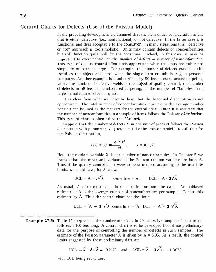
718 Chapter 17 Statistical Quality Control
Control Charts for Defects (Use of the Poisson Model) In the preceding development we assumed that the item under consideration is one that is either defective (i.e., nonfunctional) or not defective. In the latter case it is functional and thus acceptable to the consumer. In many situations this "defective or not" approach is too simplistic. Units may contain defects or nonconformities but still function quite well for the consumer. Indeed, in this case, it may be important, to exert control on the number of defects or number of nonconformities. This type of quality control effort finds application when the units are either not simplistic or perhaps large. For example, the number of defects may be quite useful as the object of control when the single item or unit is, say, a personal computer. Another example is a unit defined by 50 feet of manufactured pipeline, where the number of defective welds is the object of quality control, the number of defects in 50 feet of manufactured carpeting, or the number of "bubbles" in a large manufactured sheet of glass.
It is clear from what we describe here that the binomial distribution is not appropriate. The total number of nonconformities in a unit or the average number per unit can be used as the measure for the control chart. Often it is assumed that the number of nonconformities in a sample of items follows the Poisson distributioa. This type of chart is often called the C-chart.
Suppose that the number of defects X in one unit of product follows the Poisson distribution with parameter A. (Here t = 1 for the Poisson model.) Recall that for the Poisson distribution,
e-AA* P(X = x) = p - , x = 0,1,2
Here, the random variable X is the number of nonconformities. In Chapter 5 we learned that the mean and variance of the Poisson random variable are both A. Thus if the quality control chart were to be structured according to the usual 3u limits, wc could have, for A known,
UCL = A + 3\/A, centerline = A, LCL = A - 3\/A.
As usual, A often must come from an estimator from the data. An unbiased estimate of A is the average number of nonconformities per sample. Denote this estimate by A. Thus the control chart has the limits
UCL = A + 3 V l , centerline = A, LCL = A - 3 VX.
Example 17.5:1 Table 17.4 represents the number of defects in 20 successive samples of sheet metal rolls each 100 feet long. A control chart is to be developed from these preliminary-data for the purpose of controlling the number of defects in such samples. The estimate of the Poisson parameter A is given by A = 5.95. As a result, the control limits suggested by these preliminary data are
UCL = A + 3 \ / A ~ = 13.2678 and LCL = A - 3VA = -1.3678,
with LCL being set to zero.

17.5 Control Charts for Attributes 719
Table 17.4: Data for Example 17.5; Control Involves Number of Defects in Sheet Metal Rolls
Sample N u m b e r 1 2 3 4 5 6 7 8 9
10
Number of Defects 8 7 5 4 4 7 6 4 5 6
Sample N u m b e r 11 12 13 14 15 J6 17 18 19 20
Numbei • of Defects 3 7 5 9 7 7 8 1!
7 4
Ave. 5.95
Figure 17.9 shows a plot of the preliminary data with the control limits revealed. Table 17.5 shows additional data taken from the production process. For each
sample, the unit on which the chart was based, namely 100 feet of the metal, was inspected. The information on 20 samples is revealed. Figure 17.10 shows a plot of the additional production data. It is clear that the process is in control, at least through the period for which the data were taken. J
Table: 17.5: Additional Data from the Pnxluction Process of Example 17.5
Sample N u m b e r 1 2 3 4 5 6 7 8 9
10
N u m b e i of Defects 3 5 8 5 8 4 3 6 5 2
Sample N u m b e r 11 12 13 14 15 16 17 18 19 20
Numbe i • of Defects 7 5 9 4 6 5 3 2 1 6
In Example 17.5, we have made very clear what the sampling or inspection unit is, namely, 100 feet of metal. In many cases where the item is a specific one (e.g., a personal computer or a specific type of electronic device), the inspection unit may be a set of items. For example, the analyst may decide to use 10 computers in each subgroup and thus observe a count of the total number of defects found. Thus the preliminary sample for construction of the control chart would involve the use of several samples, each containing 10 computers. The choice of the sample size may depend on many factors. Often, we may want a sample size that will ensure an LCL that is positive.
The analyst may wish to use the average number of defects per sampling unit

720 Chapter 17 Statistical Quality Control
Figure 17.9: Preliminary data plotted on the con- Figure 17.10: Additional production data for Ex-trol chart, for Example 17.5. ample 17.5.
as the basic measure in the control chart. For example, for the case of the personal computer, let the random variable total number of defects
U total number ile:fects
be measured for each sample of, say, n = 10. We can use the method of moment-generating functions to show that U is a, Poisson random variable (see Review Exercise 17.1) if we assume that the number t>f defects per sampling unit is Poisson with parameter A. Thus the control chart for this situation is characterized by the following:
<U UCL = U + 3\J —, centerline = U, LCL = U-3\!-.
Here, of course, U is the average of the [/-values in the preliminary or base data set. The term U/n is derived from the result that
E(U) = A. Vu.r(U) = -, n
and thus U is an unbiased estimate of E(U) = A and U/n is an unbiased estimate of Vo.r(U) = X/n. This type of control chart is often called a [/-chart.
In the entire development in this se:ction we based our development of control charts on the Poisson probability model. This model has been used in combination with the 3er concept. As we have implied earlier in this chapter, the notion of 3er limits has its roots in the normal approximation, although many users feel that the concept works well as a pragmatic tool even if normality is not even approximately correct. The difficulty, of course, is that in the absence of normality, we cannot control the probability of incorrect specification of an out-of-control state. In the case of the Poisson model, when A is small the distribution is cjuite asymmetric, a condition that may produce undesirable results if we hold to the 3er approach.

17.6 Cusum Control Charts 721
17.6 Cusum Control Charts
The disadvantage with Shewhart-type control charts, developed and illustrated in the preceding sections, lies in their inability to detect small changes in the mean. A quality control mechanism that has received considerable attention in the statistics literature and usage in industry is the cumulative sum (cusum) chart. The method for the cusum chart is simple and its appeal is intuitive. It should become obvious to the reader why it is more responsive to small changes in the mean. Consider a control chart for the mean with a reference level established at value W. Consider particular observations Xi , X2,..., Xr. The first r cusums are
Si = Xx~ W
52 = S! + (X2 - W)
53 = S2 + (X3 - W)
Sr = Sr-i+(X.,.-W).
It becomes clear that the cusum is merely the accumulation of differences from the reference level. That is,
Sk = £ ) ( X i - W), A: = 1,2,.
The cusum chart is, then, a plot of Sk against time. Suppose that we consider the reference level w to be an acceptable value of the
mean p.. Clearly, if there is no shift in p, the cusum chart should be approximately horizontal, with some minor fluctuations balanced around zero. Now, if there is only a moderate change in the mean, a relatively large change in the slope of the cusum chart should result, since each new observation has a chance of contributing a shift and the measure being plotted is accumulating these shifts. Of course, the signal that the mean has shifted lies in the nature of the slope of the cusum chart. The purpose of the chart is to detect changes that are moving away from the reference level. A nonzero slope (in either direction) represents a change away from the reference level. A positive slope indicates an increase in the mean above the reference level, while a negative slope signals a decrease.
Cusum charts are often devised with a defined acceptable quality level (AQL) and a rejectable quality level (RQL) preestablished by the user. Both represent values of the mean. These may be viewed as playing roles somewhat similar to those of the null and alternative mean of hypothesis testing. Consider a situation wdiere the analyst hopes to detect an increase in the value of the process mean. We shall use the notation po for AQL and pi for RQL and let pi > po. The reference level is now set at
2
The values of Sr (r = 1,2, ) will have a negative slope if the process mean is at Po and a positive slope if the process mean is at p i .

722 Chapter 17 Statistical Quality Control
Decision Rule for Cusum Char t s
As indicated earlier, the slope of the cusum chart provides the signal of action by the quality control analyst. The decision rule calls for action if, at the rth sampling period,
dr > h,
where h is a prespecified value called the length of the decision interval and
rf = Sr — min Si. 1 <!<!-1
In other words, action is taken if the data reveal that the current cusum value exceeds by a specified amount the previous smallest cusum value.
A modification in the mechanics described above allows for ease in employing the method. We have described a procedure that plots the cusums and computes differences. A simple modification involves plotting the differences directly and allows for checking against the decision interval. The general expression for dr is quite simple. For the cusum procedure wdrere we are detecting increases in the mean,
dr = max[0,eir_i + (Xr - W)\.
The choice of the value of h is, of course, very important. We do not choose in this book to provide the many details in the literature dealing with this choice. The reader is referred to Ewan and Kemp, 1960, and Montgomery, 2000, (see the Bibliography) for a thorough discussion. One important consideration is the expected run length. Ideally, the expected run length is quite large under p — po and quite small when p = p4.
Review Exercises
17.1 Consider X\, X2,. •., Xn independent Poisson Sample X R_ random variables with parameters pi,p2, • • • ,/J-n- Use the properties of moment-generating functions to show
n
that the random variable ]T) Xi is a Poisson random i = l
n n variable with mean Y Pi and variance Y P> •
i=i i = i
17.2 Consider the following data taken on subgroups of size 5. The data contain 20 averages and ranges on the diameter (in millimeters) of an important component part of an engine. Display X- and i?.-charts. Does the process appear to be in control?
Sample X R 1 2.3972 0.0052 2 2.4191 0.0117 3 2.4215 0.0062
4 5 e 7 8 9 10 11 12 13 14 15 16 17 18 19 20
2.3917 2.4151 2.4027 2.3921 2.4171 2.3951 2.4215 2.3887 2.4107 2.4009 2.3992 2.3889 2.4107 2.4109 2.3944 2.3951 2.4015
0.0089 0.0095 0.0101 0.0091 0.0059 0.0068 0.0048 0.0082 0.0032 0.0077 0.0107 0.0025 0.0138 0.0037 0.0052 0.0038 0.0017

Review Exercises 723
17.3 Suppose for Review Exercise 17.2 that the buyer has set specifications for the part. The specifications require that the diameter fall in the range covered by 2.40000 ± 0.0100 mm. What proportion of units produced by this process will not conform to specifications?
17.4 For the situation of Review Exercise 17.2, give numerical estimates of the mean and standard deviation of the diameter for the part being manufactured in the process.
17.5 Consider the data of Table 17.1. Suppose that additional samples of size 5 are taken and tensile strength recorded. The sampling produces the following results (in pounds per square inch).
Sample X R
Sample Si
1 2 3 4 5 6 7 8 9
10
1511 1508 1522 1488 1519 1524 1519 1504 1500 1519
22 14 11 18 6
11 8 7 8
14
(a) Plot the data, using the X- and /{-charts for the preliminary data of Table 17.1.
(b) Docs the process appear to be in control? If not, explain why.
17.6 Consider an in-control process with mean p = 25 and er = 1.0. Suppose that subgroups of size 5 are used with control limits, g+ 3o/\/n, and centerline at p. Suppose that a shift occurs in the mean, and thus the new mean is p = 26.5.
(a) What is the average number of samples required (following the shift) to detect the out-of-control situation?
(b) What is the standard deviation of the number of runs required?
17.7 Consider the situation of Example 17.2. The following data are taken on additional^samples of size 5. Plot the X- and S-values on the X- and S-charts that are produced by the data in the preliminary sample. Does the process appear to be in control? Explain why or why not.
Sample S i
1 2 3 4
62.280 62.319 62.297 62.318
0.062 0.049 0.077 0.042
5 6 7 8 9
10
62.315 62.389 62.401 62.315 62.298 62.337
0.038 0.052 0.059 0.042 0.036 0.068
17.8 Samples of size 50 are taken every hour from a process producing a certain type of item that is either considered defective or not defective. Twenty samples are taken.
Sample 1 2 3 4 5 0 7 8 9
10
Number of Defective
I tems 4 3 5 3 2 2 2 1 4 3
Sample 11 12 13 14 15 16 17 18 19 20
Number of Defective
I tems 2 4 1 2 3 1 1 2 3 1
(a) Construct a control chart for control of proportion defective.
(b) Does the process appear to be in control? Explain.
17.9 For the situation of Review Exercise 17.8, suppose that additional data are collected as follows:
Sample N u m b e r of Defective I tems
1 2 3 4 5 6 7 8 9
10
3 4 2 2 3 1 3 5 7 7
Does the process appear to be in control? Explain.
17.10 A quality control effort is being attempted for a process where large steel plates are being manufactured and surface defects are of concern. The goal is to set up a quality control chart for the number of defects per plate. The data are given next page. Set up the appropriate control chart, using this sample information. Does the process appear to be in control?

724 Chapter 17 Statistical Quality Control
Number of Number of Sample Defective Sample Defective
Plot Items Plot Items
Number of Number of Sample Defective Sample Defective
Plot Items Plot Items 1 2 3 4 5
4 2 1 3 0
11 12 13 14 15
1 2 2 3 1
6 7 8 9 10
4 5 3 2 2
16 17 18 19 20
4 3 2 1 3

Chapter 18
Bayesian Statistics (Optional)
18.1 Bayesian Concepts
The classical methods of estimation that we have studied so far are based solely on information provided by the random sample. These methods essentially interpret probabilities as relative frequencies. For example, in arriving at a 95% "confidence interval for p, we interpret the statement
P(-1 .96 < Z < 1.96) = 0.95
to mean that 95% of the time in repeated experiments Z will fall between -1.96 and 1.96. Since
o/s/n.
for a normal sample with known variance, the probability statement here means that 95% of the random intervals (X - 1.96a/\/n, X + l.96o/yrn) contain the true mean p. Another approach to statistical methods of estimation is called Bayesian methodology. The main idea of the method comes from the Bayes' rule described in Section 2.8. The key difference between the Bayesian approach and classical approach (i.e., the one we have discussed in this text thus far), is that in Bayesian concepts, the parameters are viewed as random variables.
Subjective Probability Subjective probability is the foundation of Bayesian concepts. In Chapter 2, we discussed two possible approaches of probability, namely, relative frequency and indifference approaches. The first one decides a probability as a consequence of repeated experiments. For instance, to decide the free-throw percentage of a basketball player, we can record the number of shots made and the total number of attempts this player has had so far. The probability of hitting a free-throw by this player can be calculated as the ratio of these two numbers. On the other hand, if we have no knowledge of any bias of a die, the probability that a 3 will appear in the next throw will be 1/6. Such an approach in probability interpretation is based on the indifference rule.

726 Chapter 18 Bayesian Statistics (Optional)
However, in many situations, the preceding probability interpretations cannot be applied. For instance, consider the questions "What is the probability that it will rain tomorrow?" "How likely is it that this stock will go up by the end of the month?" and "What is the likelihood that two companies will be merged together?" They can hardly be interpreted by the aforementioned approaches, and the answers to these questions may be different to different people. Yet these questions are constantly asked in daily life, and the approach used to explain those probabilities is called subjective probability, which reflects one's subjective opinion.
Conditional Perspective
Recall that in Chapters 9 through 17, all statistical inferences are based on the fact that the parameters are unknown but fixed quantities, apart from that in Section 9.14, in which the parameters are treated as variables and the maximum likelihood estimates are calculated by conditioning on the data. In Bayesian statistics, the parameters are treated as random and unknown to the researcher.
Because the observed data are the only experimental results to the practitioner, statistical inference is based on the actual observed data from a given experiment. Such a view is called conditional perspective. Furthermore, in Bayesian concepts, since the parameter is treated as random, a probability distribution can be specified, by generally using the subjective probability for the parameter. Such a distribution is called a prior distribution and it usually reflects the experimenter's prior belief about the parameter. In Bayesian perspective, once an experiment is conducted and data are observed, all knowledge about a parameter is contained in the actual observed data as well as in the prior information.
Bayesian Applications
Although Bayes' rule is credited to Thomas Bayes, Bayesian applications were first introduced by French Scientist Pierre Simon Laplace, who published a paper on using Bayesian inference on the unknown binomial parameters. However, due to its sometimes complicated modeling approach and the objections from many others against the use of the subjective prior distribution, Bayesian applications were not widely accepted by researchers and scientists until early 1990s, when breakthroughs in Bayesian computational methods were achieved. Since then, Bayesian methods have been applied successfully to many fields such as engineering, agricultural, biomedical science, environmental science, and so on.
18.2 Bayesian Inferences
Consider the problem of finding a point estimate of the parameter 6 for the population with distribution /(:r| 9), given 8. Denote by n(0) the prior distribution about 0. Suppose that a random sample of size n, denoted by x = (xx,x2,..., xn), is observed.
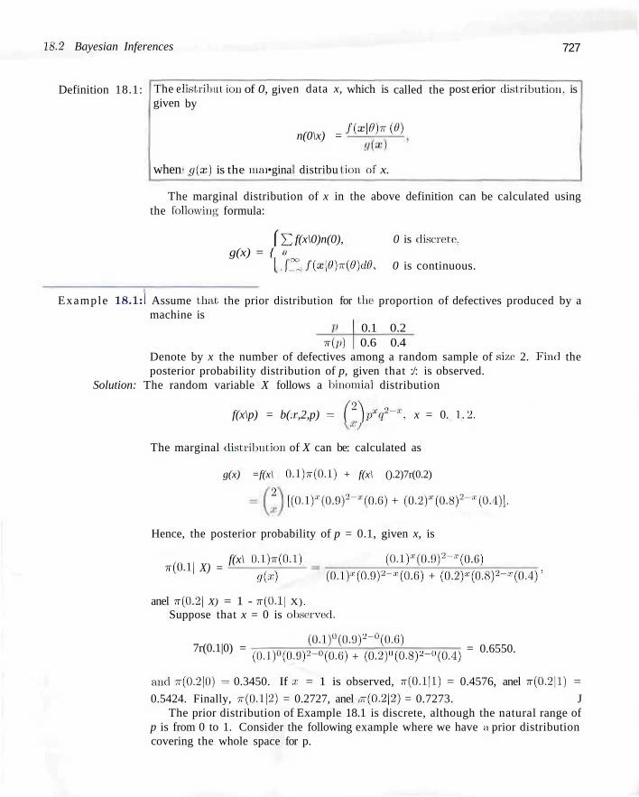
18-2 Bayesian Inferences 727
Definition 18.1: The e given
when
listril by
<iix)
ut ion of 0,
is the niai
give
•gina
n data x,
n(0\x) =
distribu
which is
f(X\0)7T
ion eif x.
called the
ie)
post erior disl ributioii. is
The marginal distribution of x in the above definition can be calculated using the following formula:
(J2 f(x\0)n(0), 0 is discrete. g(x) = { o
I (f° fix\0)rt(0) d.0, 0 is continuous.
Example 18.1:1 Assume that, the prior distribution for the proportion of defectives produced by a machine is
0.1 0.2 TT(P) 0.6 0.4
Denote by x the number of defectives among a random sample of size 2. Finel the posterior probability distribution of p, given that :/: is observed.
Solution: The random variable X follows a binomial distribution
f(x\p) = b(.r,2,p) = (2)p*q2-*, x = 0. 1.2.
The marginal distribution of X can be: calculated as
g(x) =f(x\ O.I)TT(O.I) + f(x\ ().2)7r(0.2)
2 |[(0.lHQ.9)2-s(0.6) + (0.2):n(0.8)2-''(0.4)].
Hence, the posterior probability of p = 0.1, given x, is
f(x\ O.l)Tr(O.l) ( O . l f t O J ) 2 - 3 5 ^ ) ?r(0.1| X) =
9ix) (0.1)"'(0.9)2^(0.6) + (0.2)*(0.8)2-'''-(0.4)'
anel TT(0.2| X) = 1 - TT(().1| X).
Suppose that x = 0 is observcel.
7r(0.1|0) = (0.1)°(0.9)2-°(0.6)
(0.1)°(0.9)2-°(0.6) + (0.2)(l(0.8)2-(l(0.4) = 0.6550.
and ~(0.2|0) = 0.3450. If a; = 1 is observed, TT(0.1|1) = 0.4576, anel jr(0.2jl) =
0.5424. Finally, ?r(0.112) = 0.2727, anel -(0.2|2) = 0.7273. J The prior distribution of Example 18.1 is discrete, although the natural range of
p is from 0 to 1. Consider the following example where we have a prior distribution covering the whole space for p.

728 Chapter 18 Bayesian Statistics (Optional)
Example 18.2:1 Suppose that the prior distribution of p is uniform (i.e.. 7t(p) = 1, for 0 < p < I). Use the same random variable X as in Example 18.1 to find the posterior distribution of p.
Solution: As in Example 18.1, we have
fix\p) = b(x;2,p)= Q P V ~ * , as = 0,1,2.
The marginal distribution of x can be calculated as
g(x) = j f(x\p)rt(p) dp= Q J Pxi\-P)2-X dp.
The integral above can be evaluated at each x directly as g(0) = 1/3, #(1) = 1/3 and g(2) = 1/3. Therefore, the posterior distribution of p, given x, is
nip\x)={*)pX{]~P)2~* = 3 f 2 W - P ) 8 " . 0<p<l. , 1/3 \x;
Using the posterior distribution, we can estimate the parameter(s) in a population straightforwardly.
Estimation Using the Posterior Distribution Once the posterior distribution is derived, we can easily use the summary of the posterior distribution to make inference on the population parameters. For instance, the posterior mean, median, or mode can all be used to estimate the parameter.
Example 18.3:1 Suppose that x = 1 is observed for Example 18.2. Find the posterior mean and the posterior mode.
Solution: When x — 1. the posterior distribution of p can be expressed as
7r(p|l) = 6 p ( l - p ) , for 0 < p < l .
To calculate the mean of this distribution, we need to find
1 V(i-p)*>e(i-i)-l.
To find the posterior mode, we need to obtain the value of p such that the posterior distribution is maximized. Taking derivative of Tt(p) with respect to p, we obtain 6 - 12p. Solving for p in 0 = 6 - 12p, wc obtain p = 1/2. The second derivative is — 12, which implies that the posterior mode achieves at p = 1/2. J
Bayesian methods of estimation concerning the mean p of a normal population are based on the following example.
Example 18.4:1 If x is the mean of a random sample of size n from a normal population with known variance a2, and the prior distribution of the population mean is a normal

18.2 Bayesian Inferences 729
distribution with known mean p0 and known variance IT2,, then the posterior distribution of the population mean is also a normal distribution with mean p* and the standard deviation cr*. where
P = 4 °~o + °~2/n ao + a2/n
Solution: Multiplying the density of our sample
1
a2 jn , , x + ~^y~,—T~rl'<> a n c l a —
2^-2 <7ntT
no-Q + a2
f(xx,x2,...,x»\p) = (2TV)1'/'2O7> exp
1 n
- £ j = i
Xi - p
for — oo < Xi < co and i = 1.2,..,, n by our prior
2"
7r(/i) = v/27ri 7T(7o
exp 1 (P-Po
'2 \ ao oo < p < oo,
we obtain the joint density of the random sample and the mean of the population from which the sample is selected. That is.
f(xi,x2,...,xn,p) = 1
(27r)("+1)/2ej"CT0
{-i[t(^)2+(^y x exp
In Section 8.6 we establisheel the identity
J2ixi-p)2 = irix,-x)2+n(x-p)2, i=l i=l
which enables us to write
f(xi,x2,...,xn,p) = ( 2 ^ ) ( « + l ) / 2 0 - n ( 7 o
exp 1 -££
x exp •B i= l
V2 (,, _ ,,„\2-\ n(x-p)2 (p-po) +
Completing the squares in the second exponent, we can write the joint density of the random sample and the population mean in the form
fix i, x2 x„, p) = K exp 1 (ti-li* 2 I er*
where
P = nxa2, + poa2
na2. + a2 a = no2, + a2

730 Chapter 18 Bayesian Statistics (Optional)
and K is a function of the sample values and the known parameters. The marginal distribution of the sample is then
/
OO |
• oo V27TCT'
= K\Fhto*,
and the posterior distribution is f(xi,x2,...,xn,u)
exp 1 (p-p-2
dp
it(p\xi,x2,...,xn) = g(x,i,x2,...,xn)
1
v/27r< TtO* exp 2\ a* J — oo < p < oo,
which is identified as a normal distribution with mean p* and standard deviation
a*, where p* and a* are defined above. J The central limit theorem allows us to use Example 18.4 also when we select
random samples (n > 30 for many engineering experimental cases) from nonnormal populations (the distribution is not very far from symmetric), and when the prior distribution of the mean is approximately normal.
Several comments need to be made about Example 18.4. The posterior mean p* can also be written as
* _ °o - o-2jn I1 ~ ~2~~i 2~T~X "" 2~,—TT~U0:
which is the weighted average of the sample mean x and the prior mean p0- Since both coefficients are between 0 and 1 and sum to 1, the posterior mean p* is always between x and po- This means that the posterior estimation of the location of p is influenced by both x and po- Furthermore, the weight of x depends on the prior variance as well as the variance of the sample mean. For a large sample problem (n —> co), the posterior mean p* —> x. This means that the prior mean does not play any role in estimating the population mean p using the posterior distribution. This is very reasonable since it indicates that when the amount of data is substantial, information from the data will dominate the information of p provided by the prior. On the other hand, when the prior variance is large (er2 —• cc), the posterior mean p" also goes to x. Note that for a normal distribution the larger the variance, the flatter the density function. The flatness of the normal distribution in this case means that there is almost no subjective prior information available to the parameter p. Thus, it is reasonable that the posterior estimation p* only depends on the data value x.
Now consider the posterior standard deviation a*. This value can also be written as
a2a2/n
It is obvious that the value a* is smaller than both ao and a/^/n, the prior standard deviation and the standard deviation of x, respectively. This suggests that

18.2 Bayesian Inferences 731
the posterior estimation is more accurate than both the prior and the sample data. Hence, incorporating both the data and prior information results in better posterior information than using any of the data or prior alone. This is a common phenomenon in Bayesian inference. Furthermore, to compute p* and o* by the formulas in Example 18.4, we have assumed that er2 is known. Since this is generally not the case, we shall replace er2 by the sample variance s2 whenever n > 30.
Bayesian Interval Estimation
Similar to classical confidence interval, in Bayesian analysis, we can calculate a 100(1 - o)% Bayesian interval using the posterior distribution.
Definition 18.2: The interval a < 6 < b will be called a 100(1 — a)% Bayes interval for 9 if
/
a /.oo
TT(6\X) d.0= rr(9\x) d9 = ^ . -oo Jb 2 Recall that under the frequentist approach, probability of a confidence interval,
say 95%, is interpreted as a coverage probability, which means that if an experiment is repeated again and again (with considerable unobserved data), the probability that the calculated intervals according to the rule will cover the true parameter is 95%. However, in Bayesian interval interpretation, say for a 95% interval, we can simply phrase that the probability of the unknown parameter falling into the calculated interval (only depends on the observed data) is 95%.
Example 18.5:1 Suppose that X ~ b(x;n,p) with known n = 2, and the prior distribution of p is uniform ir(p) = 1, for 0 < p < 1, find a 95% Bayes interval for p.
Solution: As in Example 18.2, when x = 0, the posterior distribution is 7r(p|0) — 3(1 —p)2, for 0 < p < 1. Thus we need to solve for a and b using Definition 18.2, which yields the following:
0.025 ,-r ./o
3 ( l - p ) 2 d p = l - ( l - a ) 3
and
0.025 /V-P)2 Jb
dp=(l- bf
The solutions to the above equations result in a = 0.0084 and b = 0.7076. Therefore, the probability that p falls into (0.0084,0.7076) is 95%. J
For the normal (population) and normal (prior) case described in Example 18.4, the posterior mean p* is the Bayes estimate of the population mean p, and a 100(1 - Q ) % Bayesian interval for p can be constructed by computing the interval
P* ~ zn/2a* <p< p* + za/2a*,
which is centered at the posterior mean and contains 100(1 — a)% of the posterior probability.

732 Chapter 18 Bayesian Statistics (Optional)
Example 18.6:1 An electrical firm manufactures light, bulbs that have a length of life that is approximately normally distributed with a standard deviation eif 100 hours. Prior experience leads us to believe that p is a value of a normal random variable with a mean po = 800 hours and a standard deviation o~o — 10 hours. If a random sample of 25 bulbs has an average life of 780 hours, find a 95%. Bayesian interval for p.
Solution: Accortling to Example 18.4, the posterior distribution of the: mean is also a normal distribution with mean
_ (25)(780)(10)2+(800)(100)2 _ ' ' (25)(10)2 + (100)2
and standard eleviation
(10)2(100)5
80. y (25)(10)2+(100)2
The 95% Bayesian interval for p is then given by
796 - 1.96V§0 < p < 796 + 1.96\/80,
or
778.5 < p. < 813.5.
Hence, we arc 95% sure that p. will be between 778.5 and 813.5. On the other hand, ignoring the prior information about p, we could proceed
as in Section 9.4 and construct the classical 95% confidence: interval
780 - (1.96) (^=V\ < p < 780 + (1.96) ' 25
or 740.8 < p < 819.2, which is seen to be wider than the corresponding Bayesian
interval. J
18.3 Bayes Estimates Using Decision Theory Framework
Using Bayesian methodology, the posterior distribution of the parameter can be obtained. Bayes estimates can also be derived using the posterior distribution when a loss function is incurred. For instance, the most popular Bayes estimate used is under the squared-error loss function, which is similar to the least squares estimates were presented in Chapter 11 in our discussion of regression analysis.
Definition 18.3: The mean of the posterior distribution TT(9\X), denote by 0*, is called the Bayes estimate of 0, under the squared-error loss function.
Example 18.7:1 Find the Bayes estimates of p, for all the values of 3S3 for Example 18.1. Solution: When x = 0, p* = (0.1)(0.6550) + (0.2)(03450) = 0.1345.
When x - I, p* = (0.1)(0.4576) + (0.2)(0.5424) = 0.1542.

18.3 Bayes Estimates Using Decision Theory Framework 733
When x = 2, p* = (0.1)(0.2727) + (0.2)(0.7273) = 0.1727. Note that the classical estimate of p is p = x/n = 0, 1/2, and 1, respectively,
for the x values at 0, 1, anel 2. The'sc classical estimates are very different from the corresponding Bayes estimates. J
Example 18.8:1 Repeat Example 18.7 in the' situation of Example 18.2. Solution: Since the posterior distribution of p can be expressed as
. W - Q g a ^ - a Q p - d - a - , »<„<i,
the Bayes estimate of p is
• i
p* = E(P\.r.) = 3 Q j p' + >(l - p)2--': dp.
which yields p* = 1/4 for x = 0, p' = 1/2 for x = 1, and p* = 3/4 for x = 2, respectively. Notice that when x = 1 is observed, the Bayes estimate and the classical estimate p arc equivalent. J
For the normal situation as described in Example 18.4, the Bayes estimate of p under the squared-error loss will be' the posterior mean p*.
Example 18.9:1 Suppose that the sampling distribution of a random variable, X, is Poisson with parameter A. Assume that the prior distribution of A follows a gamma distribution with parameters (ov,/?). Finel the Bayes estimate of A under the squared-error loss function.
Solution: The density function of A" is
f(x\X) = e " A ^ - . for a; = 0,1 x\ '
anel the prior distribution of A is
^ = ^ r \ x ' x ~ X ( ~ X ! a ' for A>0-
Hence the posterior distribution of A can be expressed by
A ' * e, \x+e*-le-(l+l//9)A n(X\x) =
r-x y e -AA«- ' e -v- \ / A ~ /•a c 'Ax+o-l r-(l + l/,3)A dx 'll x\0«r(a) "A JO * T O )
1
(1 +i/0)-(*+a)r(x+ay
which follows another gamma distribution with parameters (x + a, (1 + l/3)~l). Using Theorem 6.3, we obtain the posterior mean
I + 1/0

734 Chapter 18 Bayesian Statistics (Optional)
Since the posterior mean is the Bayes estimate under the squared-error loss, A is
our Bayes estimate. J
Exercises
18.1 Estimate the proportion of defectives being produced by the machine! in Example 18.1 if the random sample of size 2 yields 2 defectives.
18.2 Let us assume that the prior distribution for the proportion y of drinks from a vending machine that overflow is
p w(p)
0.05 0.3
0.10 0.5
0.15 0.2
If 2 of the next 9 drinks from this machine overflow, find (a) the posterior distribution for the proportion p; (b) the Bayc:s estimate of p.
18.3 Repeat Exercise 18.2 when 1 of the: next 4 drinks overflows anel the uniform prior distribution is
jr(p) = 10, 0.05 < / > < 0.15.
18.4 The developer of a new condominium complex claims that 3 out of 5 buyers will prefer a two bedroom unit, while his banker claims that it. would be more correct to say that 7 out. of 10 buyers will prefer a two-bedroom unit. In previous predictions of this type, the banker has been twice as reliable as the developer. If 12 of the next 15 condominiums solel in this complex are: two-bedroom units, Bad
(a) the posterior probabilities associated with the claims of the developer anel banker:
(b) a point estimate: of the proportion of buyers who prefer a two-bedroom unit.
18.5 The burn time for the first stage of a rocket is a normal random variable with a standard deviation of 0.8 minute. Assume a normal prior distribution for p with a mean of 8 minutes and a standard deviation of 0.2 minute. If 10 of those rockets arc fired anel the first stage has an average burn time of 9 minutes, find a 95% Bayesian interval for p.
18.0 The daily profit, from a juice vending machine placed in an office building is a value of a normal random variable with unknown mean p and variance er". Of course, the mean will vary somewhat from building to building, and the distributor feels that these average
daily profits can be'st be described by a normal distribution with mean po = $30.00 and standard deviation rrn = SI.75. If one of these juice machines, placed in a certain building, showed an average daily profit o( X = $24.90 during the first 30 days with a standard deviation of s = $2.10, find
(a) a Bayes estimate of the true average daily profit for this building;
(b) a 95% Bayesian interval of p for this buileling; (c) the probability that the average daily preifit from
the machine in this buileling is between $24.00 anel $26.00.
18.7 The mathematics department, of a large university is designing a placement test, to be given to the incoming freshman classes. Members of the: department feel that the average grade for this test will vary from one freshman class to another. This variation of the average class grade is expressed subjectively by a normal distribution with mean po = 72 and variance: exo = 5.7G.
(a) What, prior probability eloes the department assign to the actual average grade being somewhere between 71.8 and 73.4 for next year's freshman class?
(b) If the test is tried on a random sample of 100 freshman students from the next, incoming freshman class resulting in an average grade of 70 with a variance of 64, construct a 95% Bayesian interval for /(.
(c) What posterior probability should the department assign to the event of part (a)'.'
18.8 Suppose that In Example 18.6 the electrical firm eloes not. have enough prior information regarding the population mean length of life to be able to assume a normal distribution for p. The firm believes, however, that p. is surely between 770 and 830 hours and it is fell that a more realistic Bayesian approach would be to assume the prior distribution
-( / ' ) = gg, 770 < p < 8;io.
If a random sample: of 25 bulbs gives an average life of 7K0 hours, follow the steps of the proof for Example

Exercise), 735
18.4 to find the posterior distribution
n(p\xi,X2,...,X2T,).
18.9 Suppose that the time to failure T of a certain hinge is an exponential random variable with probability density
f(t) = 0c.-et, t > 0.
From prior experience we are led to believe that. 0 is a value of an exponential random variable with probability density
T!(ff) = 2e"2 0 , 0 > 0.
If we have a sample of n observations on T, show that the posterior distribution of © is a gamma distribution with parameters
a = n + 1, and ,3 = [Y^ti + 2
18.10 Suppose that a sample consisting of 5, 6, 6, 7, 5, 6, 4, 9, 3, 6 and comes from a Poisson population with mean A. Assume that the parameter A follows a gamma distribution with parameters (3,2). Under the squared-error loss, find the Bayes estimate of A.
18.11 A random variable X follows a negative binomial distribution with parameters k = 5 and p (i.e., b*(x;5,p)). Furthermore, we know that p follows a uniform distribution in the interval (0,1). Find out the Bayes estimate of p under the squared-error loss. [Hint: You may find the density function in Exercise 6.50 useful. Also, the mean of the Beta distribution with parameters (a, 3) is a/(a + /?).]

Bibliography
(6
[7;
[9;
[10;
[11
[12
[13
[14
Bartlett, M. S. and Kendall, D. G. (1946). "The Statistical Analysis of Variance Heterogeneity and Logarithmic Transformation," Journal of the Royal Statistical Society, Ser. B. 8, 128-138.
Bowker, A. H. and Lieberman. G. J. (1972). Engineering Statistics, 2nd ed. Upper Saddle River, N.J.: Prentice Hall.
Box, G. E. P. (1988). "Signal to Noise Ratios, Performance Criteria and Transformations (with discussion)," Technometrics, 30, 1-17.
Box, G. E. P. Fung, C. A. (1986). "Studies in Quality Improvement: Minimizing Transmitted Variation by Parameter Design," Report 8. University of Wisconsin-Madison, Center for Quality and Productivity Improvement.
Box, G. E. P., Hunter, W. G. and Hunter, J. S. (1978). Statistics for Experimenters. New York: John Wiley & Sons.
Brownlee, K. A. (1984). Statistical Theory and Methodology: in Science and Engineering, 2nd ed. New York: John Wiles &: Sons.
Carroll, R. J. and Ruppert, D. (1988). Transformation and Weighting in Regression. New York: Chapman and Hall.
Chatterjee, S. Hadi, A. S. and Price, B. (1999). Regression Analysis by Example, 3rd ed. New York: John Wiles & Sons.
Cook, R. D. and Weisberg, S. (1982). Residuals and Influence in Regression. New York: Chapman and Hall.
Daniel, C. and Wood, F. S. (1999). Fitting Equations to Data: Computer Analysis of Multifactor Data, 2nd ed. New York: John Wiley & Sons.
Daniel, W. W. (1989). Applied Nonparametric Statistics, 2nd ed. Belmont, California: Wadsworth Publishing Company.
Devore, J. L. (2003). Probability and Statistics for Engineering and the Sciences, 6th ed. Belmont, Calif: Duxbury Press.
Dixon, W. J. (1983). Introduction to Statistical Analysis, 4th ed. New York: McGraw-Hill.
Draper, N. R. and Smith, H. (1998). Applied Regression analysis, 3rd ed. New York: John Wiley & Sons.

738 BIBLIOGRAPHY
[15] Duncan, A. (1986). Quality Control and Industrial Statistics, 5th ed. Homewood, Illinois: Irwin.
[16] Dyer, D. D. and Keating, J. P. (1980). "On the Determination of Critical Values for Bartlett's Test," J. Am. Stat. Assoc, 75, 313-319.
[17] Ewan, W. D. and Kemp, K. W. (1960). "Sampling Inspection of Continuous Processes with No Autocorrelation between Successive Results," Biometrika, Vol. 47, 363-380.
[18] Gunst, R. F. and Mason, R. L. (1980). Regression Analysis and Its Application: A Data-Oriented Approach. New York: Marcel Dckker.
[19] Guttman, I., Wilks, S. S. and Hunter, J. S. (1971). Introductory Engineering Statistics. New York: Wiley k Sons.
[20] Hicks, C. R. and Turner, K. V. (1999). Fundamental Concepts in the Design of Experiments, 5th ed. Oxford: Oxford University Press.
[21] Hoaglin, D. C, Mosteller, F. and Tukey, J. W. (1991). Fundamentals of Exploratory Analysis of Variance. New York: Wiley &; Sons.
[22] Hocking, R.R., (1976). "The Analysis and Selection of Variables in Linear Regression," Biometrics, 32, 1-49.
[23] Hoerl, A. E. and Wennard, R. W. (1970). "Ridge Regression: Applications to Nonorthogonal Problems," Technometrics, 12, 55-67.
[24] Hogg, R. V., Craig, A. and McKean, J. W. (2004). Introduction to Mathematical Statistics, 6th ed. Upper Saddle River, N.J.: Prentice Hall.
[25] Hogg, R. V. and Ledolter, J. (1992). Applied Statistics for Engineers and Physical Scientists, 2nd ed. Upper Saddle River: N.J.: Prentice Hall.
[26] Hollander, M. and Wolfe, D. (1999). Nonparametric Statistical Methods. New York: John Wiley & Sons.
[27] Johnson, N. L. and Leone, F. C. (1977). Statistics and E:vperimental Design: In Engineering and the Physical Sciences, Vols. I and II, 2nd ed, New York: John Wiley & Sons.
[28] Kackar, R. (1985). "Off-Line Quality Control, Parameter Design, and the Taguchi Methods," Journal of Quality Technology, 17, 176-188.
[29] Koopmans, L. H. (1987). An Introduction to Contemporary Statistics, 2nd ed. Boston: Duxbury Press.
[30] Larsen, R. J. and Morris, M. L. (2000). An Introduction to Mathematical Statistics and Its Applications, 3rd ed. Upper Saddle River, N.J.: Prentice Hall.
[31] Lehmann, E. L. and D'Abrera, H. J. M. (1998). Nonparametrics: Statistical Methods Based on Ranks, rev. ed. Upper Saddle River: N.J.: Prentice Hall,
[32] Lentner, M. and Bishop, T. (1986). Design and Analysis of Experiments, 2nd ed. Blacksburg, VA: Valley Book Co.
[33] Mallows, C. L. (1973). "Some comments of Cp," Technometrics, 15, 661-675.

BIBLIOGRAPHY 739
[34;
[35;
[3e;
[37
[38
[39
[40
[41
[42
[43;
[44
[45
[46;
[47;
[48
[49
[50;
[51
McClave, J. T., Dietrich, F. H. and Sincich, T. (1997). Statistics, 7th ed. Upper Saddle River, N.J.: Prentice Hall.
Montgomery, D. C. (2000). Introduction to Statistical Quality Control, 4th ed. New York: John Wiley & Sons.
Montgomery, D. C. (2001). Design and Analysis of Experiments, 5th ed. New York: John Wiley & Sons.
Mosteller, F. and Tukey, J. (1977). Data Analysis and Regression. Reading, MA: Addison-Wesley Publishing Co.
Myers. R. H. (1990). Classical and Modern Regression with Applications, 2nd ed. Boston: Duxbury Press.
Myers, R. H., Kliuri, A. I. and Vining, G. G. (1992). "Response Surface Alternatives to the Taguchi Robust Parameter Design Approach," The American Statistician, 46, 131-139.
Myers, R. H. and Montgomery, D. C. (2002). Response Surface Methodology: Process and Product Optimization Using Designed Experiments, 2nd ed. New York: John Wiley &i Sons.
Neter, J., Wassermann, W., and Kutner, M. H. (1989). Applied Linear Regression Models, 2nd ed. Burr Ridge, Illinois: Irwin.
Noether, G. E. (1976). Introduction to Statistics: A Nonparametric Approach, 2nd ed. Boston: Houghton Mifflin Company.
Olkin, I.. Gleser, L. J. and Dernian, C. (1994). Probability Models and Applications, 2nd Ed. New York: Prentice Hall.
Ott, R. L. and Longnecker, M. T. (2000). An Introduction to Statistical Methods and Data Analysis, 5th ed. Boston: Duxbury Press.
Plackett, R. L. and Burinan, J. P. (1946). "The Design of Multifactor Experiments," Biometrika, 33, 305-325.
Ross, S. M. (2002). Introduction to Applied Probability Models, 8th ed. New York: Academic Press, Inc.
Satterthwaite, F. E. (1946). "An approximate distribution of estimates of variance components," Biometrics, 2, 110-114.
Schilling, E. G. and Nelson, P. R. (1976). "The Effect, of Nonnormality on the Control Limits of X Charts," J. Quality Tech., 8, 347-373.
Schmidt, S. R. and Launsby, R. G. (1991). Understanding Industrial Designed Experiments. Colorado Springs, CO: Air Academy Press.
Shoemaker, A. C, Tsui, K.-L., and Wu, C. F. J. (1991). "Economical Experimentation Methods for Robust Parameter Design," Technometrics, 33, 415-428,
Snedecor, G. W. and Cochran, W. G. (1989). Statistical Methods, 8th ed. Allies, Iowa: The Iowa State University Press.

740 BIBLIOGRAPHY
[52] Steel, R. G. D., Torrie, J. H. and Dickey, D. A. (1996). Principles and Procedures of Statistics: A Biometrical Approach, 3rd ed. New York: McGraw-Hill.
[53] Taguchi, G. (1991). Introduction to Quality Engineering. White Plains, N.Y.: Unipub/Kraus International.
[54] Taguchi, G. and Wu, Y. (1985). Introduction to Off-Line Quality Control. Nagoya, Japan: Central Japan Quality Control Association.
[55] Thompson, W. O. and Cady, F. B. (1973). Proceedings of the University of Kentucky Conference on Regression with a Large Number of Predictor Variables. Lexington, Kentucky: University of Kentucjy press.
[56] Tukey, J. W. (1977). Exploratory Data Analysis. Reading, MA: Addison-Wesley Publishing Co.
[57] Vining, G. G. and Myers, R. H. (1990). "Combining Taguchi and Response Surface Philosophies: A Dual Response Approach." Journal of Quality Technology, 22, 38-45.
[58] Welch, W. J., Yu, T. K., Kang, S. M. and Sacks, J. (1990). "Computer Experiments for Quality Control by Parameter Design," Journal of Quality Technology, 22, 15-22.
[59] Winer, B. J. (1991). Statistical Principles In Experimental Design, 3rd ed. New York: McGraw-Hill.

Appendix A
Statistical Tables and Proofs

742 Appendix A Statistical Tables and Proofs
r Table A . l Binomial Probability Sums YI b(x;n,p)
x=0
n r 1 0
1
2 0 1 2
3 0 1 2 3
4 0 1 2 3 4
5 0 1 2 3 4 5
6 0 1 2 3 4 5 6
7 0 1 2 3 4 5 6 7
0.10
0.9000 1.0000
0.8100 0.9900 1.0000
0.7290 0.9720 0.9990 1.0000
0.6561 0.9477 0.9963 0.9999 1.0000
0.5905 0.9185 0.9914 0.9995 1.0000 1.0000
0.5314 0.8857 0.9842 0.9987 0.9999 1.0000 1.0000
0.4783 0.8503 0.9743 0.9973 0.9998 1.0000
0.20
0.8000 1.0000
0.6400 0.9600 1.0000
0.5120 0.8960 0.9920 1.0000
0.4096 0.8192 0.9728 0.9984 1.0000
0.3277 0.7373 0.9421 0.9933 0.9997 1.0000
0.2621 0.6554 0.9011 0.9830 0.9984 0.9999 1.0000
0.2097 0.5767 0.8520 0.9667 0.9953 0.9996 1.0000
0.25
0.7500 1.0000
0.5625 0.9375 1.0000
0.4219 0.8438 0.9844 1.0000
0.3164 0.7383 0.9492 0.9961 1.0000
0.2373 0.6328 0.8965 0.9844 0.9990 1.0000
0.1780 0.5339 0.8306 0.9624 0.9954 0.9998 1.0000
0.1335 0.4449 0.7564 0.9294 0.9871 0.9987 0.9999 1.0000
0.30
0.7000 1.0000
0.4900 0.9100 1.0000
0.3430 0.7840 0.9730 1.0000
0.2401 0.6517 0.9163 0.9919 1.0000
0.1681 0.5282 0.8369 0.9692 0.9976 1.0000
0.1176 0.4202 0.7443 0.9295 0.9891 0.9993 1.0000
0.0824 0.3294 0.6471 0.8740 0.9712 0.9962 0.9998 1.0000
I 0.40
0.6000 1.0000
0.3600 0.8400 1.0000
0.2160 0.6480 0.9360 1.0000
0.1296 0.4752 0.8208 0.9744 1.0000
0.0778 0.3370 0.6826 0.9130 0.9898 1.0000
0.0467 0.2333 0.5443 0.8208 0.9590 0.9959 1.0000
0.0280 0.1586 0.4199 0.7102 0.9037 0.9812 0.9984 1.0000
» 0.50
0.5000 1.0000
0.2500 0.7500 1.0000
0.1250 0.5000 0.8750 1.0000
0.0625 0.3125 0.6875 0.9375 1.0000
0.0313 0.1875 0.5000 0.8125 0.9688 1.0000
0.0156 0.1094 0.3438 0.6563 0.8906 0.9844 1.0000
0.0078 0.0625 0.2266 0.5000 0.7734 0.9375 0.9922 1.0000
0.60
0.4000 1.0000
0.1600 0.6400 1.0000
0.0640 0.3520 0.7840 1.0000
0.0256 0.1792 0.5248 0.8704 1.0000
0.0102 0.0870 0.3174 0.6630 0.9222 1.0000
0.0041 0.0410 0.1792 0.4557 0.7667 0.9533 1.0000
0.0016 0.0188 0.0963 0.2898 0.5801 0.8414 0.9720 1.0000
0.70
0.3000 1.0000
0.0900 0.5100 1.0000
0.0270 0.2160 0.6570 1.0000
0.0081 0.0837 0.3483 0.7599 1.0000
0.0024 0.0308 0.1631 0.4718 0.8319 1.0000
0.0007 0.0109 0.0705 0.2557 0.5798 0.8824 1.0000
0.0002 0.0038 0.0288 0.1260 0.3529 0.6706 0.9176 1.0000
0.80
0.2000 1.0000
0.0400 0.3600 1.0000
0.0080 0.1040 0.4880 1.0000
0.0016 0.0272 0.1808 0.5904 1.0000
0.0003 0.0067 0.0579 0.2627 0.6723 1.0000
0.0001 0.0016 0.0170 0.0989 0.3446 0.7379 1.0000
0.0000 0.0004 0.0047 0.0333 0.1480 0.4233 0.7903 1.0000
0.90
0.1000 1.0000
0.0100 0.1900 1.0000
0.0010 0.0280 0.2710 1.0000
0.0001 0.0037 0.0523 0.3439 1.0000
0.0000 0.0005 0.0086 0.0815 0.4095 1.0000
0.0000 0.0001 0.0013 0.0159 0.1143 0.4686 1.0000
0.0000 0.0002 0.0027 0.0257 0.1497 0.5217 1.0000

Table A.l Binomial Probability Table 743
r Table A . l (continued) Binomial Probability Sums J2 °ix'ini'P)
x=0
n r 8 0
1 2 3 4 5 6 7 8
9 0 1 2 3 4 5 6 7 8 9
10 0 1 2 3 4 5 6 7 8 9
10
11 0 1 2 3 4 5 6 7 8 9 10 11
0.10
0.4305
0.8131 0.9619
0.9950
0.9996 1.0000
0.3874
0.7748
0.9470
0.9917
0.9991 0.9999
1.0000
0.3487
0.7361
0.9298 0.9872
0.9984
0.9999 1.0000
0.3138
0.6974 0.9104 0.9815
0.9972
0.9997
1.0000
0.20
0.1678
0.5033
0.7969 0.9437
0.9896 0.9988
0.9999
1.0000
0.1342
0.4362
0.7382
0.9144 0.9804
0.9969 0.9997
1.0000
0.1074
0.3758
0.6778
0.8791 0.9672
0.9936
0.9991 0.9999
1.0000
0.0859
0.3221 0.6174
0.8389 0.9496 0.9883
0.9980
0.9998 1.0000
0.25
0.1001
0.3671 0.6785
0.8862
0.9727
0.9958
0.9996
1.0000
0.0751
0.3003
0.6007
0.8343
0.9511 0.9900
0.9987
0.9999
1.0000
0.0563
0.2440 0.5256
0.7759
0.9219
0.9803
0.9965
0.9996
1.0000
0.0422
0.1971 0.4552 0.7133
0.8854
0.9657 0.9924
0.9988 0.9999
1.0000
0.30
0.0576
0.2553
0.5518
0.8059
0.9420
0.9887 0.9987
0.9999
1.0000
0.0404
0.1960
0.4628 0.7297
0.9012
0.9747
0.9957
0.9996
1.0000
0.0282
0.1493
0.3828
0.6496
0.8497
0.9527
0.9894
0.9984
0.9999 1.0000
0.0198
0.1130 0.3127 0.5696
0.7897
0.9218
0.9784
0.9957 0.9994
1.0000
P 0.40
0.0168
0.1064
0.3154
0.5941
0.8263 0.9502
0.9915
0.9993
1.0000
0.0101
0.0705
0.2318
0.4826
0.7334
0.9006
0.9750
0.9962
0.9997
1.0000
0.0060
0.0464
0.1673
0.3823
0.6331
0.8338 0.9452
0.9877
0.9983 0.9999
1.0000
0.0036
0.0302 0.1189" 0.2963
0.5328
0.7535
0.9006
0.9707 0.9941
0.9993
1.0000
0.50
0.0039
0.0352
0.1445 0.3633
0.6367
0.8555
0.9648 0.9961
1.0000
0.0020
0.0195 0.0898
0.2539 0.5000
0.7461
0.9102
0.9805
0.9980
1.0000
0.0010
0.0107
0.0547
0.1719 0.3770
0.6230
0.8281
0.9453
0.9893
0.9990 1.0000
0.0005 0.0059 0.0327 •
0.1133 0.2744
0.5000
0.7256 0.8867 0.9673
0.9941
0.9995
1.0000
0.60
0.0007
0.0085
0.0498
0.1737 0.4059
0.6846
0.8936 0.9832
1.0000
0.0003
0.0038
0.0250 0.0994
0.2666
0.5174
0.7682
0.9295
0.9899
1.0000
0.0001
0.0017
0.0123
0.0548 0.1662
0.3669
0.6177 0.8327
0.9536
0.9940 1.0000
0.0000 0.0007
0.0059 0.0293 0.0994
0.2465 0.4672
0.7037 0.8811
0.9698 0.9964
1.0000
0.70
0.0001
0.0013
0.0113 0.0580 0.1941
0.4482
0.7447 0.9424
1.0000
0.0000
0.0004
0.0043 0.0253
0.0988
0.2703 0.5372
0.8040
0.9596
1.0000
0.0000
0.0001 0.0016
0.0106 0.0473
0.1503
0.3504
0.6172
0.8507
0.9718
1.0000
0.0000
0.0006 0.0043
0.0216
0.0782
0.2103 0.4304 0.6873
0.8870 0.9802 1.0000
0.80
0.0000
0.0001 0.0012
0.0104
0.0563 0.2031
0.4967 0.8322
1.0000
0.0000
0.0003 0.0031
0.0196
0.0856
0.2618
0.5638
0.8658
1.0000
0.0000 0.0001
0.0009 0.0064
0.0328
0.1209
0.3222
0.6242
0.8926 1.0000
0.0000 0.0002
0.0020
0.0117 0.0504
0.1611 0.3826
0.6779 0.9141
1.0000
0.90
0.0000
0.0004
0.0050 0.0381
0.1869
0.5695
1.0000
0.0000 0.0001
0.0009
0.0083
0.0530
0.2252
0.6126
1.0000
0.0000 0.0001
0.0016
0.0128 0.0702
0.2639
0.6513 1.0000
--.
0.0000
0.0003 0.0028 0.0185
0.0896 0.3026 0.6862
1.0000
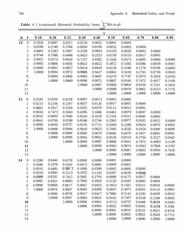
744 Appendix A Statistical Tables and Proofs
r
Table A . l (continued) Binomial Probability Sums YI 0ix:.n-.P) x=0
n r 12 0
1 2 3 4 5 6 7 8 9
10 11 12
13 0 1 2 3 4 5 6 7 8 9
10 11 12 13
14 0 1 2 3 4 5 6 7 8 9
10 11 12 13 14
0.10 0.2824 0.6590 0.8891 0.9744 0.9957 0.9995 0.9999 1.0000
0.2542 0.6213 0.8661 0.9658 0.9935 0.9991 0.9999 1.0000
0.2288 0.5846 0.8416 0.9559 0.9908 0.9985 0.9998 1.0000
0.20 0.0687 0.2749 0.5583 0.7946 0.9274 0.9806 0.9961 0.9994 0.9999 1.0000
0.0550 0.2336 0.5017 0.7473 0.9009 0.9700 0.9930 0.9988 0.9998 1.0000
0.0440 0.1979 0.4481 0.6982 0.8702 0.9561 0.9884 0.9976 0.9996 1.0000
0.25
0.0317 0.1584 0.3907 0.6488 0.8424 0.9456 0.9857 0.9972 0.9996 1.0000
0.0238 0.1267 0.3326 0.5843 0.7940 0.9198 0.9757 0.9944 0.9990 0.9999 1.0000
0.0178 0.1010 0.281 T 0.5213 0.7415 0.8883 0.9617 0.9897 0.9978 0.9997 1.0000
0.30
0.0138 0.0850 0.2528 0.4925 0.7237 0.8822 0.9614 0.9905 0.9983 0.9998 1.0000
0.0097 0.0637 0.2025 0.4206 0.6543 0.8346 0.9376 0.9818 0.9960 0.9993 0.9999 1.0000
0.0068 0.0475 0.1608 0.3552 0.5842 0.7805 0.9067 0.9685 0.9917 0.9983 0.9998 1.0000
V 0.40
0.0022 0.0196 0.0834 0.2253 0.4382 0.6652 0.8418 0.9427 0.9847 0.9972 0.9997 1.0000
0.0013 0.0126 0.0579 0.1686 0.3530 0.5744 0.7712 0.9023 0.9679 0.9922 0.9987 0.9999 1.0000
0.0008 0.0081 0.0398 0.1243 0.2793 0.1859 0.6925 0.8499 0.9417 0.9825 0.9961 0.9994 0.9999 1.0000
0.50
0.0002 0.0032 0.0193 0.0730 0.1938 0.3872 0.6128 0.8062 0.9270 0.9807 0.9968 0.9998 1.0000
0.0001 0.0017 0.0112 0.0461 0.1334 0.2905 0.5000 0.7095 0.8666 0.9539 0.9888 0.9983 0.9999 1.0000
0.0001 0.0009 0.0065 0.0287 0.0898 0.2120 0.3953 0.6047 0.7880 0.9102 0.9713 0.9935 0.9991 0.9999 1.0000
0.60
0.0000 0.0003 0.0028 0.0153 0.0573 0.1582 0.3348 0.5618 0.7747 0.9166 0.9804 0.9978 1.0000
0.0000 0.0001 0.0013 0.0078 0.0321 0.0977 0.2288 0.4256 0.6470 0.8314 0.9421 0.9874 0.9987 1.0000
0.0000 0.0001 0.0006 0.0039 0.0175 0.0583 0.1501 0.3075 0.5141 0.7207 0.8757 0.9602 0.9919 0.9992 1.0000
0.70
0.0000 0.0002 0.0017 0.0095 0.0386 0.1178 0.2763 0.5075 0.7472 0.9150 0.9862 1.0000
0.0000 0.0001 0.0007 0.0040 0.0182 0.0624 0.1654 0.3457 0.5794 0.7975 0.9363 0.9903 1.0000
0.0000 0.0002 0.0017 0.0083 0.0315 0.0933 0.2195 0.4158 0.6448 0.8392 0.9525 0.9932 1.0000
0.80
0.0000 0.0001 0.0006 0.0039 0.0194 0.0726 0.2054 0.4417 0.7251 0.9313 1.0000
0.0000 0.0002 0.0012 0.0070 0.0300 0.0991 0.2527 0.4983 0.7664 0.9450 1.0000
0.0000 0.0004 0.0024 0.0116 0.0439 0.1298 u.3018 0.5519 0.8021 0.9560 1.0000
0.90
0.0000 0.0001 0.0005 0.0043 0.0256 0.1109 0.3410 0.7176 1.0000
0.0000 0.0001 0.0009 0.0065 0.0342 0.1339 0.3787 0.7458 1.0000
0.0000 0.0002 0.0015 0.0092 0.0441 0.1584 0.4154 0.7712 1.0000

Table A.l Binomial Probability Table 745
r Table A . l (continued) Binomial Probability Sums Y2 Kxin>P)
x=a
n r 15 0
1 2 3 4 5 6 7 8 9 10 11 12 13 14 15
16 0 1 2 3 4 5 6 7 8 9 10 11 12 13 14 15 16
0.10
0.2059 0.5490 0.8159 0.9444 0.9873 0.9978 0.9997 1.0000
0.1853 0.5147 0.7892 0.9316 0.9830 0.9967 0.9995 0.9999 1.0000
0.20
0.0352 0.1671 0.3980 0.6482 0.8358 0.9389 0.9819 0.9958 0.9992 0.9999 1.0000
0.0281 0.1407 0.3518 0.5981 0.7982 0.9183 0.9733 0.9930 0.9985 0.9998 1.0000
0.25
0.0134 0.0802 0.2361 0.4613 0.6865 0.8516 0.9434 0.9827 0.9958 0.9992 0.9999 1.0000
0.0100 0.0635 0.1971 0.4050 0.6302 0.8103 0.9204 0.9729 0.9925 0.9984 0.9997 1.0000
0.30
0.0047 0.0353 0.1268 0.2969 0.5155 0.7216 0.8089 0.9500 0.9848 0.9963 0.9993 0.9999 1.0000
0.0033 0.0261 0.0994 0.2459 0.4499 0.6598 0.8247 0.9256 0.9743 0.9929 0.9984 0.9997 1.0000
P 0.40
0.0005 0.0052 0.0271 0.0905 0.2173 0.4032 0.6098 0.7869 0.9050 0.9662 0.9907 0.9981 0.9997 1.0000
0.0003 0.0033 0.0183 0.0651 0.1666 0.3288 0.5272 0.7161 0.8577 0.9417 0.9809 0.9951 0.9991 0.9999 1.0000
0.50
0.0000 0.0005 0.0037 0.0176 0.0592 0.1509 0.3036 0.5000 0.6964 0.8491 0.9408 0.9824 0.9963 0.9995 1.0000
0.0000 0.0003 0.0021 0.0106 0.0384 0.1051 0.2272 0.4018 0.5982 0.7728 0.8949 0.9616 0.9894 0.9979 0.9997 1.0000
0.60
0.0000 0.0003 0.0019 0.0093 0.0338 0.0950 0.2131 0.3902 0.5968 0.7827 0.9095 0.9729 0.9948 0.9995 1.0000
0.0000 0.0001 0.0009 0.0049 0.0191 0.0583 0.1423 0.2839 0.4728 0.6712 0.8334 0.9349 0.9817 0.9967 0.9997 1.0000
0.70
0.0000 0.0001 0.0007 0.0037 0.0152 0.0500 0.1311 0.2784 0.4845 0.7031 0.8732 0.9647 0.9953 1.0000
0.0000 0.0003 0.0016 0.0071 0.0257 0.0744 0.1753 0.3402 0.5501 0.7541 0.9006 0.9739 0.9967 1.0000
0.80
0.0000 0.0001 0.0008 0.0042 0.0181 0.0611 0.1642 0.3518 0.6020 0.8329 0.9648 1.0000
0.0000 0.0002 0.0015 0.0070 0.0267 0.0817 0.2018 0.4019 0.6482 0.8593 0.9719 1.0000
0.90
0.0000 0.0003 0.0022 0.0127 0.0556 0.1841 0.4510 0.7941 1.0000
0.0000 0.0001 0.0005 0.0033 0.0170 0.0684 0.2108 0.4853 0.8147 1.0000

746 Appendix A Statistical Tables and Proofs
r
Table A.l (continued) Binomial Probability Sums YL °ix-n^p) x=Q
n r 17 0
1 2 3 4 5 6 7 8 9 10 11 12 13 14 15 16 17
18 0 1 2 3 4 5 6 7 8 9 10 11 12 13 14 15 16 17 18
0.10
0.1668 0.4818 0.7618 0.9174 0.9779 0.9953 0.9992 0.9999 1.0000
0.1501 0.4503 0.7338 0.9018 0.9718 0.9936 0.9988 0.9998 1.0000
0.20
0.0225 0.1182 0.3096 0.5489 0.7582 0.8943 0.9623 0.9891 0.9974 0.9995 0.9999 1.0000
0.0180 0.0991 0.2713 0.5010 0.7164 0.8671 0.9487 0.9837 0.9957 0.9991 0.9998 1.0000
0.25
0.0075 0.0501 0.1637 0.3530 0.5739 0.7653 0.8929 0.9598 0.9876 0.9969 0.9994 0.9999 1.0000
0.0056 0.0395 0.1353 0.3057 0.5187 0.7175 0.8610 0.9431 0.9807 0.9946 0.9988 0.9998 1.0000
0.30
0.0023 0.0193 0.0774 0.2019 0.3887 0.5968 0.7752 0.8954 0.9597 0.9873 0.9968 0.9993 0.9999 1.0000
0.0016 0.0142 0.0600 0.1646 0.3327 0.5344 0.7217 0.8593 0.9404 0.9790 0.9939 0.9986 0.9997 1.0000
I 0.40
0.0002 0.0021 0.0123 0.0464 0.1260 0.2639 0.4478 0.6405 0.8011 0.9081 0.9652 0.9894 0.9975 0.9995 0.9999 1.0000
0.0001 0.0013 0.0082 0.0328 0.0942 0.2088 0.3743 0.5634 0.7368 0.8653 0.9424 0.9797 0.9942 0.9987 0.9998 1.0000
i
0.50
0.0000 0.0001 0.0012 0.0064 0.0245 0.0717 0.1662 0.3145 0.5000 0.6855 0.8338 0.9283 0.9755 0.9936 0.9988 0.9999 1.0000
0.0000 0.0001 0.0007 0.0038 0.0154 0.0481 0.1189 0.2403 0.4073 0.5927 0.7597 0.8811 0.9519 0.9846 0.9962 0.9993 0.9999 1.0000
0.60
0.0000 0.0001 0.0005 0.0025 0.0106 0.0348 0.0919 0.1989 0.3595 0.5522 0.7361 0.8740 0.9536 0.9877 0.9979 0.9998 1.0000
0.0000 0.0002 0.0013 0.0058 0.0203 0.0576 0.1347 0.2632 0.4366 0.6257 0.7912 0.9058 0.9672 0.9918 0.9987 0.9999 1.0000
0.70
0.0000 0.0001 0.0007 0.0032 0.0127 0.0403 0.1046 0.2248 0.4032 0.6113 0.7981 0.9226 0.9807 0.9977 1.0000
0.0000 0.0003 0.0014 0.0061 0.0210 0.0596 0.1407 0.2783 0.4656 0.6673 0.8354 0.9400 0.9858 0.9984 1.0000
0.80
0.0000 0.0001 0.0005 0.0026 0.0109 0.0377 0.1057 0.2418 0.4511 0.6904 0.8818 0.9775 1.0000
0.0000 0.0002 0.0009 0.0043 0.0163 0.0513 0.1329 0.2836 0.4990 0.7287 0.9009 0.9820 1.0000
0.90
0.0000 0.0001 0.0008 0.0047 0.0221 0.0826 0.2382 0.5182 0.8332 1.0000
0.0000 0.0002 0.0012 0.0064 0.0282 0.0982 0.2662 0.5497 0.8499 1.0000

Table A.l Binomial Probability Table 747
r
Table A . l (continued) Binomial Probability Sums YI b(x;n,p) x=a
n r 19 0
1 2 3 4 5 6 7 8 9 10 11 12 13 14 15 16 17 18 19
20 0 1 2 3 4 5 6 7 8 9 10 11 12 13 14 15 16 17 18 19 20
0.10
0.1351 0.4203 0.7054 0.8850 0.9648 0.9914 0.9983 0.9997 1.0000
0.1216 0.3917 0.6769 0.8670 0.9568 0.9887 0.9976 0.9996 0.9999 1.0000
0.20
0.0144 0.0829 0.2369 0.4551 0.6733 0.8369 0.9324 0.9767 0.9933 0.9984 0.9997 1.0000
0.0115 0.0692 0.2061 0.4114 0.6296 0.8042 0.9133 0.9679 0.9900 0.9974 0.9994 0.9999 1.0000
0.25
0.0042 0.0310 0.1113 0.2631 0.4654 0.6678 0.8251 0.9225 0.9713 0.9911 0.9977 0.9995 0.9999 1.0000
0.0032 0.0243 0.0913 0.2252 0.4148 0.6172 0.7858 0.8982 0.9591 0.9861 0.9961 0.9991 0.9998 1.0000
0.30
0.0011 0.0104 0.0462 0.1332 0.2822 0.4739 0.6655 0.8180 0.9161 0.9674 0.9895 0.9972 0.9994 0.9999 1.0000
0.0008 0.0076 0.0355 0.1071 0.2375 0.4164 0.6080 0.7723 0.8867 0.9520 0.9829 0.9949 0.9987 0.9997 1.0000
P 0.40
0.0001 0.0008 0.0055 0.0230 0.0696 0.1629 0.3081 0.4878 0.6675 0.8139 0.9115 0.9648 0.9884 0.9969 0.9994 0.9999 1.0000
0.0000 0.0005 0.0036 0.0160 0.0510 0.1256 0.2500 0.4159 0.5956 0.7553 0.8725 0.9435 0.9790 0.9935 0.9984 0.9997 1.0000
0.50
0.0000 0.0004 0.0022 0.0096 0.0318 0.0835 0.1796 0.3238 0.5000 0.6762 0.8204 0.9165 0.9682 0.9904 0.9978 0.9996 1.0000
0.0000 0.0002 0.0013 0.0059 0.0207 0.0577 0.1316 0.2517 0.4119 0.5881 0.7483 0.8684 0.9423 0.9793 0.9941 0.9987 0.9998 1.0000
0.60
0.0000 0.0001 0.0006 0.0031 0.0116 0.0352 0.0885 0.1861 0.3325 0.5122 0.6919 0.8371 0.9304 0.9770 0.9945 0.9992 0.9999 1.0000
0.0000 0.0003 0.0016 0.0065 0.0210 0.0565 0.1275 0.2447 0.4044 0.5841 0.7500 0.8744 0.9490 0.9840 0.9964 0.9995 1.0000
0.70
0.0000 0.0001 0.0006 0.0028 0.0105 0.0326 0.0839 0.1820 0.3345 0.5261 0.7178 0.8668 0.9538 0.9896 0.9989 1.0000
0.0000 0.0003 0.0013 0.0051 0.0171 0.0480 0.1133 0.2277 0.3920 0.5836 0.7625 0.8929 0.9645 0.9924 0.9992 1.0000
0.80
0.0000 0.0003 0.0016 0.0067 0.0233 0.0676 0.1631 0.3267 0.5449 0.7631 0.9171 0.9856 1.0000
0.0000 0.0001 0.0006 0.0026 0.0100 0.0321 0.0867 0.1958 0.3704 0.5886 0.7939 0.9308 0.9885 1.0000
0.90
0.0000 0.0003 0.0017 0.0086 0.0352 0.1150 0.2946 0.5797 0.8649 1.0000
0.0000 0.0001 0.0004 0.0024 0.0113 0.0432 0.1330 0.3231 0,6083 0.8784 1.0000

748 Appendix A Statistical Tables and Proofs
Table A.2 Poisson Probability Sums YI Pix\ M) x=0
r 0 1 2 3 4 5 6
0.1
0.9048 0.9953 0.9998 1.0000
0.2
0.8187 0.9825 0.9989 0.9999 1.0000
0.3
0.7408 0.9631 0.9964 0.9997 1.0000
0.4
0.6703 0.9384 0.9921 0.9992 0.9999 1.0000
P 0.5
0.6065 0.9098 0.9856 0.9982 0.9998 1.0000
0.6
0.5488 0.8781 0.9769 0.9966 0.9996 1.0000
0.7
0.4966 0.8442 0.9659 0.9942 0.9992 0.9999 1.0000
0.8
0.4493 0.8088 0.9526 0.9909 0.9986 0.9998 1.0000
0.9
0.4066 0.7725 0.9371 0.9865 0.9977 0.9997 1.0000
r 0 1 2 3 4 5
6 7 8 9 10
11 12 13 14 15 16
1.0 0.3679 0.7358 0.9197 0.9810 0.9963 0.9994
0.9999 1.0000
1.5 0.2231 0.5578 0.8088 0.9344 0.9814 0.9955
0.9991 0.9998 1.0000
2.0 0.1353 0.4060 0.6767 0.8571 0.9473 0.9834
0.9955 0.9989 0.9998 1.0000
2.5 0.0821 0.2873 0.5438 0.7576 0.8912 0.9580
0.9858 0.9958 0.9989 0.9997 0.9999
1.0000
M 3.0
0.0498 0.1991 0.4232 0.6472 0.8153 0.9161
0.9665 0.9881 0.9962 0.9989 0.9997
0.9999 1.0000
3.5 0.0302 0.1359 0.3208 0.5366 0.7254 0.8576
0.9347 0.9733 0.9901 0.9967 0.9990
0.9997 0.9999 1.0000
4.0
0.0183 0.0916 0.2381 0.4335 0.6288 0.7851
0.8893 0.9489 0.9786 0.9919 0.9972
0.9991 0.9997 0.9999 1.0000
4.5
0.0111 0.0611 0.1736 0.3423 0.5321 0.7029
0.8311 0.9134 0.9597 0.9829 0.9933
0.9976 0.9992 0.9997 0.9999 1.0000
5.0 0.0067 0.0404 0.1247 0.2650 0.4405 0.6160
0.7622 0.8666 0.9319 0.9682 0.9863
0.9945 0.9980 0.9993 0.9998 0.9999 1.0000

Table A.2 Poisson Probability Table 749
Table A.2 (continued) Poisson Probability Sums YL Pix'-> u) x=0
r
0 1 2 3 4 5
6 7 8 9 10
11 12 13 14 15
16 17 18 19 20
21 22 23 24
5.5 0.0041 0.0266 0.0884 0.2017 0.3575 0.5289
0.6860 0.8095 0.8944 0.9462 0.9747
0.9890 0.9955 0.9983 0.9994 0.9998
0.9999 1.0000
6.0 0.0025 0.0174 0.0620 0.1512 0.2851 0.4457
0.6063 0.7440 0.8472 0.9161 0.9574
0.9799 0.9912 0.9964 0.9986 0.9995
0.9998 0.9999 1.0000
6.5 0.0015 0.0113 0.0430 0.1118 0.2237 0.3690
0.5265 0.6728 0.7916 0.8774 0.9332
0.9661 0.9840 0.9929 0.9970 0.9988
0.9996 0.9998 0.9999 1.0000
7.0 0.0009 0.0073 0.0296 0.0818 0.1730 0.3007
0.4497 0.5987 0.7291 0.8305 0.9015
0.9467 0.9730 0.9872 0.9943 0.9976
0.9990 0.9996 0.9999 1.0000
/* 7.5
0.0006 0.0047 0.0203 0.0591 0.1321 0.2414
0.3782 0.5246 0.6620 0.7764 0.8622
0.9208 0.9573 0.9784 0.9897 0.9954
0.9980 0.9992 0.9997 0.9999
8.0
0.0003 0.0030 0.0138 0.0424 0.0996 0.1912
0.3134 0.4530 0.5925 0.7166 0.8159
0.8881 0.9362 0.9658 0.9827 0.9918
0.9963 0.9984 0.9993 0.9997 0.9999
1.0000
8.5 0.0002 0.0019 0.0093 0.0301 0.0744 0.1496
0.2562 0.3856 0.5231 0.6530 0.7634
0.8487 0.9091 0.9486 0.9726 0.9862
0.9934 0.9970 0.9987 0.9995 0.9998
0.9999 1.0000
9.0
0.0001 0.0012 0.0062 0.0212 0.0550 0.1157
0.2068 0.3239 0.4557 0.5874 0.7060
0.8030 0.8758 0.9261 0.9585 0.9780
0.9889 0.9947 0.9976 0.9989 0.9996
0.9998 0.9999 1.0000
9.5
0.0001 0.0008 0.0042 0.0149 0.0403 0.0885
0.1649 0.2687 0.3918 0.5218 0.6453
0.7520 0.8364 0.8981 0.9400 0.9665
0.9823 0.9911 0.9957 0.9980 0.9991
0.9996 0.9999 0.9999 1.0000

750 Appendix A Statistical Tables and Proofs
Table A.2 (continued) Poisson Probability Sums YI Pixi ll) x=0
r
0 1 2 3 4 5
6 7 8 9
10
11 12 13 14 15
16 17 18 19 20
21 22 23 24 25
26 27 28 29 30
31 32 33 34 35
36 37
10.0
0.0000 0.0005 0.0028 0.0103 0.0293 0.0671
0.1301 0.2202 0.3328 0.4579 0.5830
0.6968 0.7916 0.8645 0.9165 0.9513
0.9730 0.9857 0.9928 0.9965 0.9984
0.9993 0.9997 0.9999 1.0000
11.0 0.0000 0.0002 0.0012 0.0049 0.0151 0.0375
0.0786 0.1432 0.2320 0.3405 0.4599
0.5793 0.6887 0.7813 0.8540 0.9074
0.9441 0.9678 0.9823 0.9907 0.9953
0.9977 0.9990 0.9995 0.9998 0.9999
1.0000
12.0
0.0000 0.0001 0.0005 0.0023 0.0076 0.0203
0.0458 0.0895 0.1550 0.2424 0.3472
0.4616 0.5760 0.6815 0.7720 0.8444
0.8987 0.9370 0.9626 0.9787 0.9884
0.9939 0.9970 0.9985 0.9993 0.9997
0.9999 0.9999 1.0000
13.0
0.0000 0.0002 0.0011 0.0037 0.0107
0.0259 0.0540 0.0998 0.1658 0.2517
0.3532 0.4631 0.5730 0.6751 0.7636
0.8355 0.8905 0.9302 0.9573 0.9750
0.9859 0.9924 0.9960 0.9980 0.9990
0.9995 0.9998 0.9999 1.0000
P 14.0
0.0000 0.0001 0.0005 0.0018 0.0055
0.0142 0.0316 0.0621 0.1094 0.1757
0.2600 0.3585 0.4644 0.5704 0.6694
0.7559 0.8272 0.8826 0.9235 0.9521
0.9712 0.9833 0.9907 0.9950 0.9974
0.9987 0.9994 0.9997 0.9999 0.9999
1.0000
15.0
0.0000 0.0002 0.0009 0.0028
0.0076 0.0180 0.0374 0.0699 0.1185
0.1848 0.2676 0.3632 0.4657 0.5681
0.6641 0.7489 0.8195 0.8752 0.9170
0.9469 0.9673 0.9805 0.9888 0.9938
0.9967 0.9983 0.9991 0.9996 0.9998
0.9999 1.0000
16.0
0.0000 0.0001 0.0004 0.0014
0.0040 0.0100 0.0220 0.0433 0.0774
0.1270 0.1931 0.2745 0.3675 0.4667
0.5660 0.6593 0.7423 0.8122 0.8682
0.9108 0.9418 0.9633 0.9777 0.9869
0.9925 0.9959 0.9978 0.9989 0.9994
0.9997 0.9999 0.9999 1.0000
17.0
0.0000 0.0002 0.0007
0.0021 0.0054 0.0126 0.0261 0.0491
0.0847 0.1350 0.2009 0.2808 0.3715
0.4677 0.5640 0.6550 0.7363 0.8055
0.8615 0.9047 0.9367 0.9594 0.9748
0.9848 0.9912 0.9950 0.9973 0.9986
0.9993 0.9996 0.9998 0.9999 1.0000
18.8
0.0000 0.0001 0.0003
0.0010 0.0029 0.0071 0.0154 0.0304
0.0549 0.0917 0.1426 0.2081 0.2867
0.3751 0.4686 0.5622 0.6509 0.7307
0.7991 0.8551 0.8989 0.9317 0.9554
0.9718 0.9827 0.9897 0.9941 0.9967
0.9982 0.9990 0.9995 0.9998 0.9999
0.9999 1.0000

Table A.3 Normal Probability Table 751
Table A.3 Areas under the Normal Curve
.00 .01 .02 .03 .04 .05 .06 .07 .08 .09 3.4 3.3 3.2 3.1 3.0
2.9 2.8 2.7 2.6 2.5
2.4 2.3 2.2 2.1 2.0
1.9 1.8 1.7 1.6 1.5
1.4 1.3 1.2 1.1 1.0
0.9 0.8 0.7 0.6 0.5
0.4 0.3 0.2 0.1 0.0
0.0003
0.0005
0.0007
0.0010
0.0013
0.0019
0.0026
0.0035
0.0047 0.0062
0.0082
0.0107 0.0139
0.0179
0.0228
0.0287
0.03.59
0.0446 0.0548
0.0668
0.0808 0.0968
0.1151
0.1357 0.1587
0.1841 0.2119
0.2420
0.2743 0.3085
0.3446
0.3821
0.4207
0.4602 0.5000
0.0003
0.0005
0.0007
0.0009
0.0013
0.0018
0.0025 0.0034
0.0045
0.0060
0.0080 0.0104
0.0136 0.0171
0.0222
0.0281
0.0351
0.0436 0.0537
0.0655
0.0793
0.0951
0.1131
0.1335
0.1562
0.1814
0.2090
0.2389
0.2709 0.3050
0.3409
0.3783
0.4168 0.4562
0.4960
0.0003
0.0005
0.0006
0.0009
0.0013
0.0018
0.0024
0.0033 0.0044
0.0059
0.0078
0.0102 0.0132
0.0170
0.0217
0.0274
0.0344
0.0427 0.0526 0.0643
0.077S
0.0934
0.1112
0.1314 0.1539
0.1788 0.2061
0.2358
0.2676 0.3015
0.3372
0.3745 0.4 L29
0.4522 0.4920
0.0003
0.0004
0.0006
0.0009 0.0012
0.0017
0.0023
0.0032
0.0043
0.0057
0.0075 0.0099
0.0129
0.0166 0.0212
0.0208
0.0336
0.0418
0.0516 0.0630
0.0764
0.0918
0.1093 0.1292
0.1515
0.1762
0.2033
0.2327
0.2643
0.2981
0.3336
0.3707
0.4090
0.4483 0.4880
0.0003
0.0004
0.0006
0.0008 0.0012
0.00 IG
0.0023
0.(1031 0.0041
0.0055
0.0073
0.0096 0.0125
0.0162
0.0207
0.0262
0.0329
0.0409
0.0505
0.0018
0.0749
0.0901
0.1075
0.1271
0.1192
0.1736
0.2005
0.2296
0.2611 0.2946
0.3300
0.3669
0.4052
0.4443 0.4840
0.0003 0.0004
0.0006 0.0008
0.0011
0.0016
0.0022
0.0030 0.0040
0.0054
0.0071 0.0094
0.0122
0.0158 0.0202
0.0256 0.0322
0.0401
0.0495 0.0606
0.0735
0.0885
0.1056 0.1251
0.1469
0.1711
0.1977
0.2206
0.2578 0.2912
0.3264
0.3632
0.4013 0.4404
0.4801
0.0003
0.0004
0.0006 0.0008
0.0011
0.0015
0.0021 0.0029
0.0039
0.0052
0.0069
0.0091
0.0119
0.0154
0.0197
0.0250
0.0314
0.0392
0.0485
0.0591
0.0721
0.0869
0.1038
11.1230
0.1446
0.1685
0.1949
0.2236
0.2546 0.2877
0.3228
0.3594
0.3974
0.4364
0.4761
0.0003
0.0004
0.0005
0.0008
0.0011
0.0015
0.0021
0.0028 0.0038
0.0051
0.0068
0.0089
0.0110
0.0150 0.0192
0.0244
0.0307
0.0384
0.0475
0.0582
0.0708 0.0853
0.1020
0.1210
0.1423
0.1660 0.1922
0.2206
0.2514
0.2843
0.3192
0.3557 0.3936
0.4325 0.4721
0.0003
0.0004
0.0005
0.0007
0.0010
0.0(114
0.0020
0.0027
0.0037
0.0049
0.0066
0.0087
0.0113
0.0146
0.0188
0.0239 0.0301
0.0375
0.0465 0.0571
0.0694
0.0838
0.1003 0.1190
0.1401
0.1635 0.1894
0.2177
0.2483 0.2810
0.3156
0.3520
0.3897
0.4286
0.4681
0.0002
0.0003
0.0005
0.0007
0.0010
0.001 1
0.0019
0.0026 0.0036
0.0048
0.0064 0.0084
0.0110
0.0143
0.0183
0.0233
0.0294
0.0367
0.0455
0.0559
0.0681 0.0823
0.0985
0.1170
0.1379
0.1611
0.1807
0.2148
0.2451 0.2776
0.3121 0.3483
0.3859
0.4247 0.4641

752 Appendix A Statistical Tables and Proofs
Table A.3 (continued) Areas under the Normal Curve:
z 0.0 0.1 0.2 0.3 0.4
0.5 0.6 0.7 0.8 0.9
1.0 1.1 1.2 1.3 1.4
1.5 1.6 1.7 1.8 1.9
2.0 2.1 2.2 2.3 2.4
2.5 2.6 2.7 2.8 2.9
3.0 3.1 3.2 3.3 3.4
.00
0.5000
0.5398
0.5793
0.6179 0.6554
0.6915
0.7257 0.7580
0.7881
0.8159
0.8413
0.8643 0.8849
0.9032
0.9192
0.9332
0.9452 0.9554
0.9641
0.9713
0.9772
0.9821
0.9861
0.9893
0.9918
0.9938 0.9953
0.9965
0.9974
0.9981
0.9987 0.9990 0.9993
0.9995
0.9997
.01
0.5040
0.5138 0.5832
0.6217 0.6591
0.6950 0.7291
0.7611
0.7910
0.8186
0.8438
0.8665
0.8869
0.9049
0.9207
0.9345
0.9463 0.9564
0.9649
0.9719
0.9778
0.9826 0.9864
0.9896
0.9920
0.9940
0.9955
0.9966
0.9975 0.9982
0.9987 0.9991 0.9993
0.9995 0.9997
.02
0.5080
0.5478
0.5871
0.6255 0.6628
0.6985 0.7324
0.7642
0.7939 0.8212
0.8461 0.8686
0.8888
0.9066 0.9222
0.9357
0.9474
0.9573
0.9656
0.9726
0.9783
0.9830
0.9868
0.9898
0.9922
0.9941
0.9956
0.9967
0.9976
0.9982
0.9987 0.9991 0.9994
0.9995
0.9997
.03
0.5120
0.5517
0.5910
0.6293 0.6664
0.7019
0.7357
0.7673
0.7967 0.8238
0.8485
0.8708
0.8907 0.9082
0.1)236
0.9370
0.9484
0.9582
0.9664
0.9732
0.9788
0.9834
0.9871
0.9901
0.9925
0.9943
0.9957 0.9968
0.9977
0.9983
0.9988 0.9991 0.0994
0.9996
0.9097
.04
0.5160
0.5557
0.5948
0.6331
0.6700
0.7054
0.7389 0.7701
0.7995
0.8264
0.8508
0.8729 0.8925
0.9099
0.9251
0.9382
0.9495
0.9591
0.9671 0.9738
0.9793
0.9838
0.9875 0.9904
0.9927
0.9945 0.9959
0.9969
0.9977
0.9984
0.9988 0.9992
0.9994
0.9996
0.9997
.05
0.5199
0.5596
0.5987
0.6368
0.6736
0.7088 0.7422
0.7734
0.8023
0.8289
0.8531
0.8749 0.8944
0.9115
0.9265
0.9394
0.9505 0.9599
0.9G78
0.9744
0.9798
0.9842
0.9878
0.9906
0.9929
0.9946
0.9960
0.9970
0.9978 0.9984
0.9989 0.9992 0.9994
0.9996
0.9997
.06
0.5239
0.5636
0.6026
0.6406
0.6772
0.7123 0.7454
0.7764
0.8051
0.8315
0.8554
0.8770
0.8962
0.9131 0.9279
0.9406
0.9515
0.9608
0.9686
0.9750
0.9803 0.9846
0.9881
0.9909
0.9931
0.9948
0.9961
0.9971 0.9979
0.9985
0.9989 0.9992 0.9994
0.9996
0.9997
.07
0.5279
0.5675 0.6064
0.6443
0.6808
0.7157 0.7486
0.7794
0.8078
0.8340
0.8577 0.8790
0.8980
0.9147 0.9292
0.9418
0.9525
0.9616
0.9693
0.9756
0.9808 0.9850
0.9884
0.9911
0.9932
0.9949
0.9962
0.9972
0.9979
0.9985
0.9989 0.9992
0.9995
0.9996
0.9997
.08
0.5319
0.5714
0.6103
0.6480 0.6844
0.7190
0.7517
0.7823
0.8106
0.8365
0.8599
0.8810
0.8997 0.9162
0.9306
0.9429
0.9535
0.9625
0.9699
0.9761
0.9812
0.9854
0.9887
0.9913
0.9934
0.9951 0.9963
0.9973
0.9980
0.9986
0.9990 0.9993 0.9995
0.9996
0.9997
.09
0.5359
0.5753 0.6141
0.6517 0.6879
0.7224
0.7549
0.7852
0.8133
0.8389
0.8621
0.8830
0.9015
0.9177
0.9319
0.9441
0.9545
0.9633
0.9706
0.9767
0.9817
0.9857
0.9890 0.9916
0.9936
0.9952
0.9964
0.9974
0.9981
0.9986
0.9990 0.9993 0.9995
0.9997
0.9998

Table A.4 Student t-Distribtiiion Probability Table 753
T a b l e A . 4 Critical Values
v
1 2 3 1
5
6 7 8
i) 10
11 12 13 11 15
16 17 IS 1!) 20
21 22 23 24 25
26 27 28 29 30
40 60
120 CO
0.40
0.325 0.289 0.277 0.271 0.267
0.265 0.263 0.262 0.261 0.260
0.260 0.259 0.259 0.258 0.258
0.258 0.257 0.257 0.257 0.257
0.257 0.256 0.256 0.256 0.256
0.256 0.256 0.256 0.256 0.256
0.255 0.254 0.254 0.253
0.30
0.727 0.617 0.584 0.569 0.559
0.553 0.549 0.546 0.543 0.542
0.540 0.539 0.538 0.537 0.536
0.535 0.534 0.534 0.533 0.533
0.532 0.532 0.532 0.531
0.531
0.531
0.531 0.530 0.530 0.530
0.529 0.527 0.526 0.524
of the f-Dist;
0.20
1.376 1.061 0.978 0.941 0.920
0.906 0.896 0.889 0.883 0.879
0.876 0.873 0.870 0.868 0.866
0.865 0.863 0.862 0.861 0.860
0.859 0.858 0.858 0.857 0.856
0.850 0.855 0.855 0.854 0.854
0.851 0.848 0.845 0.842
dilution
Q
0.15
1.963 1.386 1.250 1.190 1.156
1.134 1.119 1.108 1.100 1.093
1.088 1.083 1.079 1.076 1.074
1.071 1.069 1.067 1.1)66 1.064
1.063 1.061 1.060 1.059 1.058
1.058 1.057 1.056 1.055 1.055
1.050 1.015 1.041 1.036
0.10
3.078 1.886 1.638 1.533 1.476
1.440 1.415 1.397 1.383 1.372
1.363 1.356 1.350 1.345 1.341
1.337 1.333 1.330 1.328 1.325
1.323 1.321 1.319 1.318 1.316
1.315 1.314
1.313 1.311 1.310
1.303 1.296 1.289 1.282
0
0.05
6.314 2.920 2.353 2.132 2.015
1.943 1.895 1.860 1.833 1.812
1.796 1.782 1.771 1.761 1,753
1.746 1.740 1.734 1.729 1.725
1.721 1.717 1.714 1.711 1.70S
1.706 1.703 1.701 1.699 1.697
1.684 1.671 1.658 1.645
;,
0 .025
12.706 4.303 3.182 2.770 2.571
2.447 2.365 2.306 2.262 2.228
2.201 2.179 2.1 GO 2.145 2.131
2.120 2.110 2.101 2.093 2.086
2.080 2.074 2.069 2.064 2.060
2.056 2.052 2.048 2.045 2.042
2.021 2.000 1.980 1.960

754 Appendix A Statistical Tables and Proofs
Table A.4 (continued) Critical Values of the f-Distribution
V
1 2 3 4 5
6 7 8 9
10
11 12 13 14 15
16 17 18 19 20
21 22 23 24 25
26 27 28 29 30
40 60
120 CO
0.02 15.894 4.849 3.482 2.999 2.757
2.612 2.517 2.449 2.398 2.359
2.328 2.303 2.282 2.264 2.249
2.235 2.224 2.214 2.205 2.197
2.189 2.183 2.177 2.172 2.167
2.162 2.158 2.154 2.150 2.147
2.123 2.099 2.076 2.054
0.015
21.205 5.643 3.896 3.298 3.003
2.829 2.715 2.634 2.574 2.527
2.491 2.461 2.436 2.415 2.397
2.382 2.368 2.356 2.346 2.336
2.328 2.320 2.313 2.307 2.301
2.296 2.291 2.286 2.282 2.278
2.250 2.223 2.196 2.170
0.01 31.821 6.965 4.541 3.747 3.365
3.143 2.998 2.896 2.821 2.764
2.718 2.681 2.650 2.624 2.602
2.583 2.567 2.552 2.539 2.528
2.518 2.508 2.500 2.492 2.485
2.479 2.473 2.467 2.462 2.457
2.423 2.390 2.358 2.326
a 0.0075
42.433 8.073 5.047 4.088 3.634
3.372 3.203 3.085 2.998 2.932
2.879 2.836 2.801 2.771 2.746
2.724 2.706 2.689 2.674 2.661
2.649 2.639 2.629 2.620 2.612
2.605 2.598 2.592 2.586 2.581
2.542 2.504 2.468 2.432
0.005 63.656 9.925 5.841 4.604 4.032
3.707 3.499 3.355 3.250 3.169
3.106 3.055 3.012 2.977 2.947
2.921 2.898 2.878 2.861 2.845
2.831 2.819 2.807 2.797 2.787
2.779 2.771 2.763 2.756 2.750
2.704 2.660 2.617 2.576
0.0025 127.321
14.089 7.453 5.598 4.773
4.317 4.029 3.833 3.690 3.581
3.497 3.428 3.372 3.326 3.286
3.252 3.222 3.197 3.174 3.153
3.135 3.119 3.104 3.091 3.078
3.067 3.057 3.047 3.038 3.030
2.971 2.915 2.860 2.807
0.0005
636.578 31.600 12.924 8.610 6.869
5.959 5.408 5.041 4.781 4.587
4.437 4.318 4.221 4.140 4.073
4.015 3.965 3.922 3.883 3.850
3.819 3.792 3.768 3.745 3.725
3.707 3.689 3.674 3.660 3.646
3.551 3.460 3.373 3.290

Table A.5 Chi-Squ-ared Distribution. Probability Tabic 755
T a b l e A . 5 Critical Values of the Chi-Squared Distribution 0 A
a
v 0 .995 0.99 0 .98 0 .975 0 .95 0 .90 0 .80 0 .75 0 .70 0 .50
1 2 3 4 5
6 7 8 9
10
11 12 13 14 15
16 17 18 19 20
21 22 23 24 25
20 27 28 29 30
40 50 60
0.04393 0.0100 0.0717 0.207 0.412
0.676 0.989 1.344 1.735 2.1.56
2.603 3.074 3.565 4.075 4.601
5.142 5.697 6.265 6.844 7.434
8.034 8.643 9.260 9.886
10.520
11.160 11.808 12.461 13.121 13.787
20.707 27.991 35.534
().()3157 0.0201
0.115 0.297 0.554
0.872 1.239 1.647 2.088 2.558
3.053 3.571 4.107 4.660 5.229
5.812 6.408 7.015 7.633 8.260
8.897 9.542
10.196 10.856 11.524
12.198 12.878 13.565 11.256 14.953
22.164 29.707 37.485
0.03628 0.0404 0.185 0.429 0.752
1.134 1.561 2.032 2.532 3.059
3.609 4.178 4.765 5.368 5.985
6.614 7.255 7.906 8.567 9.237
9.915 10.600 11.293 11.992 12.697
13.409 14.125 14.847 15.574 16.306
23.838 31.664 39.699
0.03982 0.0506 0.216 0.484 0.831
1.237 1.690 2.1.80 2.700 3.247
3.816 4.404 5.009 5.629 6.262
6.908 7.564 8.231 8.907 9.591
10.283 10.982 11.689 12.401 13.120
13.844 14.573 15.308 16.047 16.791
24.433 32.357 40,182
0.00393 0.103 0.352 11.71 1 1.145
1.635 2.167 2.733 3.325 3.940
4.575
5.226 5.892 6.571 7.261
7.962 8.672 9.390
10.117 10.851
11.591 12.338 13.091 13.848 14.611
15.379 16.151 16.928 17.708 18.493
26.509 34.764 43.188
0.0158 0.211 0.584 1.064 1.610
2.204 2.833 3.490 4.168 4.865
5.578 6.304 7.041 7.790 8.547
9.312 10.085 10.865 11.651 12.443
13.240 14.041 14.848 15.659 16.473
17.292 "1.8.114 18.939 19.768 20.599
29.051 37.689 46.459
0.0642 0.446 1.005 1.649 2.343
3.070 3.822 4.594 5.380 6.179
6.989
7.807 8.634 9.467
10.307
11.152 12.002 12.857 13.716 14.578
15.445 16.311 17.187 18.062 18.940
19.820 20.703 21.588 22.475 23.364
32.345 41.449 50.641
0.102 0.575 1.213 1.923 2.675
3.455 4.255 5.071 5.899 6.737
7.584 8.438 9.299
10.165 11.037
11.912 12.792 13.675 14.562 15.452
16.344 17.240 18.137 19.037 19.939
20.843 21.749 22.657 23.567 24.478
33.66 42.942 52.294
0.148 0.713 1.424 2.195 3.000
3.828 4.671 5.527 6.393 7.267
8.148 9.031 9.926
10.821 11.721
12.624 13.531 14.440 15.352 16.266
17.182 18.101 19.021 19.943 20.867
21.792 22.719 23.647 24.577 25.508
34.872 44.313 53.809
0.455 1.386 2.366 3.357 4.351
5.348 6.346 7.344 8.343 9.342
10.341 11.340 12.340 13.339 14.339
15.338 16.338 17.338 18.338 19.337
20.337 21.337 22.337 23.337 24.337
25.336 26.336 27.336 28.336 29.336
39.335 49.335 59.335

756 Appendix A Statistical Tables and Proofs
Table A.5 (continued) Critical Values of the Chi-Squared Distribution
V
1 2 3 4 5
6 7 8 9 10
11 12 13 14 15
16 17 18 19 20
21 22 23 24 25
26 27 28 29 30
40 50 60
0.30
1.074
2.408
3.665
4.878 6.064
7.231
8.383
9.524
10.656
11.781
12.899 14.011
15.119
16.222
17.322
18.418
19.511
20.601
21.689
22.775
23.858
24.939
26.018 27.096
28.172
29.246
30.319
31.391 32.461
33.530
44.165
54.723
65.226
0.25
1.323
2.773
4.108 5.385
6.626
7.841
9.037
10.219
11.389
12.549
13.701
14.845 15.984
17.117
18.245
19.369
20.489
21.605
22.718
23-828
24.935
26.039 27.141
28.241
29.339
30.435
31.528
32.620 33.711
34.800
45.616 56.334
66.981
0.20
1.642
3.219 4.642
5.989
7.289
8.558
9.803
11.030 12.242
13.442
14.631
15.812
16.985
18.151
19.311
20.465
21.615
22.760
23.900
25.038
26.171
27.301
28.429 29.553
30.675
31.795 32.912
34.027
35.139
36.250
47.269 58.164
68.972
0.10
2.706
4.605 6.251
7.779
9.236
10.645
12.017
13.362
14.684
15.987
17.275 18.549
19.812
21.064
22.307
23.542
24.769
25.989 27.204
28.412
29.615
30.813
32.007
33.196 34.382
35.563
36.741
37.916 39.087
40.256
51.805
63.167
74.397
0.05
3.841
5.991
7.815
9.488
11.070
12.592
14.067
15.507
16.919 18.307
19.675
21.026
22.362
23.685
24.996
26.296
27.587
28.869 30.144
31.410
32.671
33.924
35.172
36.415 37.652
38.885
40.113
41.337 42.557
43.773
55.758
67.505 79.082
a 0.025
5.024
7.378
9.348
11.143
12.832
14.449
16.013
17.535
19.023
20.483
21.920
23.337
24.736
26.119
27.488
28.845
30.191
31.526 32.852
34.170
35.479
36.781
38.076 39.364
40.646
41.923
43.195 44.461
45.722
46.979
59.342
71.420 83.298
0.02
5.412
7.824
9.837
11.668
13.388
15.033
16.622
18.168
19.679
21.161
22.618
24.054
25.471
26.873
28.259
29.633
30.995
32.346 33.687
35.020
36.343
37.659
38.968
40.270 41.566
42.856
44.140
45.419 46.693
47.962
60.436
72.613 84.58
0.01
6.635
9.210
11.345
13.277
15.086
16.812
18.475
20.090 21.666
23.209
24.725
26.217
27.688 29.141
30.578
32.000
33.409
34.805
36.191
37.566
38.932
40.289
41.638
42.980 44.314
45.642
46.963 48.278
49.588
50.892
63.691
76.154
88.379
0.005
7.879
10.597
12.838 14.860
16.750
18.548
20.278
21.955 23.589
25.188
26.757
28.300
29.819
31.319
32.801
34.267
35.718 37.156
38.582
39.997
41.401
42.796
44.181
45.558
46.928
48.290
49.645
50.994
52.335 53.672
66.766
79.490 91.952
0.001
10.827
13.815
16.266 18.466
20.515
22.457
24.321
26.124
27.877
29.588
31.264
32.909
34.527
36.124
37.698
39.252
40.791 42.312
43.819
45.314
46.796
48.268
49.728
51.179
52.619
54.051
55.475
56.892 58.301
59.702
73.403
86.660 99.608

Table A.(> F-Distribution Probability Table
Table A.6* Critical Values of the F-Distribution
757
fo.or,ici,i>2) Vi
1 161.45 199.50 2 18.51 19.00 3 10.13 9.55 4 7.71 6.94 5 6.61 5.79
6 5.99 5.14 7 5.59 4.74 8 5.32 4.46 9 5.12 4.26
10 4.96 4.10
11 4.84 3.98 12 4.75 3.89 13 4.67 3.81 14 4.60 3.74 15 4.54 3.68
16 4.49 3.63 17 4.45 3.59 18 1.41 3.55 19 4.38 3.52 20 4.35 3.49
21 4.32 3.47 22 4.30 3.44 23 4.28 3.42 24 4.26 3.40 25 4.21 3.39
26 4.23 3.37 27 4.21 3.35 28 4.20 3.34 29 4.18 3.33 30 4.17 3.32
40 4.08 3.23 60 4.00 3.15
120 3.92 3.07 oc. 3.84 3.00
* Reproduced from Table
215.71 19.16 9.28 6.59 5,11
4.76 4.35 4.07 3.86 3.71
3.59 3.49 3.41 3.34 3.29
3.24 3.20 3.16 3.13 3.10
3.07 3.05 3.03 3.01 2.99
2.98 2.96 2.95 2.93 2.92
2.84 2.76 2.68 2.60
18 of Biomt Pearson and the Biometrika Trustees.
224.58 19.25 9.12 6.39 5.19
4.53 4.12 3.84 3.63 3.48
3.36 3.26 3.18 3.11 3.06
3.01 2.96 2.93 2.90 2.87
2.84 2.82 2.80 2.78 2.76
2.74 2.73 2.71 2.70 2.69
2.61 2.53 2.45 2.37
trika Table
230.16 233.99 19.30 19.33 9.0J 8.94 6.26 6.16 5.05 4.95
4.39 4.28 3.97 3.87 3.69 3.58 3.48 3.37 3.33 3.22
3.20 3.09 3.11 3.00 3.03 2.92 2.96 2.85 2.90 2.79
2.85 2.74 2.81 2.70 2.77 2.66 2.74 2.63 2.71 2.60
2.68 2,57 2.66 2,55 2.64 2,53 2.62 2,51 2.GO 2.49
2,59 2.47 2,57 2.46 2.56 2.45 2.55 2.43 2,53 2.42
2.45 2.34 2.37 2.25 2.29 2.18 2.21 2.10
> for Statisticians, Vo
236.77 19.35 8.89 6.09 4.88
4.21 3.79 3.50 3.29 3.14
3.01 2.91 2.83 2.76 2.71
2.66 2,61 2.58 2.5-1 2.51
2.49 2.46 2.44 2.42 2.40
2.39 2.37 2.36 2.35 2.33
2.25 2.17 2.09 2.01
. I. by
238.88 19.37 8.85 6.04 4.82
4.15 3.73 3.44 3.23 3.07
2.95 2.85 2.77 2.70 2.64
2,59 2,55 2,51 2.48 2.45
2.42 2.40 2.37 2.36 2.34
2.32 2,31 2.29 2.28 2.27
2. J 8 2.10 2.02 1.94
permission
240.54 19.38 8.81 6.00 4.77
4.10 3.68 3.39 3.18 3.02
2.90 2.80 2.71 2.65 2,59
2,54 2.49 2.46 2,12 2.39
2.37 2.34 2.32 2.30 2.28
2.27 2.25 2.24 2.22 2.21
2.12 2.04 1.96 1.88
of E S .

758 Appendix A Statistical Tables and Proofs
Table A.6 (continued) Critical Values of the F-Distribution
v2
1 2 3 4 5
6 7 8 9
10
11 12 13 14 15
16 17 18 19 20
21 22 23 24 25
26 27 28 29 30
40 60
120 CO
10
241.88 19.40 8.79 5.96 4.74
4.06 3.64 3.35 3.14 2.98
2.85 2.75 2.67 2.60 2.54
2.49 2.45 2.41 2.38 2.35
2.32 2.30 2.27 2.25 2.24
2.22 2.20 2.19 2.18 2.16
2.08 1.99 1.91 1.83
12
243.91 19.41 8.74 5.91 4.68
4.00 3.57 3.28 3.07 2.91
2.79 2.69 2.60 2.53 2.48
2.42 2.38 2.34 2.31 2.28
2.25 2.23 2.20 2.18 2.16
2.15 2.13 2.12 2.10 2.09
2.00 1.92 1.83 1.75
15
245.95 19.43 8.70 5.86 4.62
3.94 3.51 3.22 3.01 2.85
2.72 2.62 2.53 2.46 2.40
2.35 2.31 2.27 2.23 2.20
2.18 2.15 2.13 2.11 2.09
2.07 2.06 2.04 2.03 2.01
1.92 1.84 1.75 1.67
20
248.01 19.45 8.66 5.80 4.56
3.87 3.44 3.15 2.94 2.77
2.65 2.54 2.46 2.39 2.33
2.28 2.23 2.19 2.16 2.12
2.10 2.07 2.05 2,03 2.01
1.99 1.97 1.96 1.94 1.93
1.84 1.75 1.66 1.57
/ o . 0 5 ( ^ 1
24
249.05 1 19.45 8.64 5.77 4.53
3.84 3.41 3.12 2.90 2.74
2.61 2.51 2.42 2.35 2.29
2.24 2.19 2.15 2.11 2.08
2.05 2.03 2.01 1.98 1.96
1.95 1.93 1.91 1.90 1.89
1.79 1.70 1.61 1.52
, « 2 )
30
250.10 19.46 8.62 5.75 4.50
3.81 3.38 3.08 2.86 2.70
2.57 2.47 2.38 2.31 2.25
2.19 2.15 2.11 2.07 2.04
2.01 1.98 1.96 1.94 1.92
1.90 1.88 1.87 1.85 1.84
1.74 1.65 1.55 1.46
40
251.14 19.47 8.59 5.72 4.46
3.77 3.34 3.04 2.83 2.66
2.53 2.43 2.34 2.27 2.20
2.15 2.10 2.06 2.03 1.99
1.96 1.94 1.91 1.89 1.87
1.85 1.84 1.82 1.81 1.79
1.69 1.59 1.50 1.39
60
252.20 19.48 8.57 5.69 4.43
3.74 3.30 3.01 2.79 2.62
2.49 2.38 2.30 2.22 2.16
2.11 2.06 2.02 1.98 1.95
1.92 1.89 1.86 1.84 1.82
1.80 1.79 1.77 1.75 1.74
1.64 1.53 1.43 1.32
120 253.25
19.49 8.55 5.66 4.40
3.70 3.27 2.97 2.75 2.58
2.45 2.34 2.25 2.18 2.11
2.06 2.01 1.97 1.93 1.90
1.87 1.84 1.81 1.79 1.77
1.75 1.73 1.71 1.70 1.68
1.58 1.47 1.35 1.22
CO
254.31 19.50 8.53 5.63 4.36
3.67 3.23 2.93 2.71 2.54
2.40 2.30 2.21 2.13 2.07
2.01 1.96 1.92 1.88 1.84
1.81 1.78 1.76 1.73 1.71
1.69 1.67 1.65 1.64 1.62
1.51 1.39 1.25 1.00

Table A.6 F-Distribution Probability Table 759
Table A.6 (continued) Critical Values of the F-Distribution
v2
1 2 3 4 5
6 7 8 9
10
11 12 13 14 15
16 17 18 19 20
21 22 23 24 25
26 27 28 29 30
40 60
120 CO
1
4052.18 98.50 34.12 21.20 16.26
13.75 12.25 11.26 10.56 10.04
9.65 9.33 9.07 8.86 8.68
8.53 8.40 8.29 8.18 8.10
8.02 7.95 7.88 7.82 7.77
7.72 7.68 7.64 7.60 7.56
7.31 7.08 6.85 6.63
2
4999.50 99.00 30.82 18.00 13.27
10.92 9.55 8.65 8.02 7.56
7.21 6.93 6.70 6.51 6.36
6.23 6.11 6.01 5.93 5.85
5.78 5.72 5.66 5.61 5.57
5.53 5.49 5.45 5.42 5.39
5.18 4.98 4.79 4.61
3
5403.35 99.17 29.46 16.69 12.06
9.78 8.45 7.59 6.99 6.55
6.22 5.95 5.74 5.56 5.42
5.29 5.18 5.09 5.01 4.94
4.87 4.82 4.76 4.72 4.68
4.64 4.60 4.57 4.54 4.51
4.31 4.13 3.95 3.78
fo.oiivi,v2) 4
5624.58 99.25 28.71 15.98 11.39
9.15 7.85 7.01 6.42 5.99
5.67 5.41 5.21 5.04 4.89
4.77 4.67 4.58 4.50 4.43
4.37 4.31 4.26 4.22 4.18
4.14 4.11 4.07 4.04 4.02
3.83 3.65 3.48 3.32
5
5763.65 99.30 28.24 15.52 10.97
8.75 7.46 6.63 6.06 5.64
5.32 5.06 4.86 4.69 4.56
4.44 4.34 4.25 4.17 4.10
4.04 3.99 3.94 3.90 3.85
3.82 3.78 3.75 3.73 3.70
3.51 3.34 3.17 3.02
6
5858.99 99.33 27.91 15.21 10.67
8.47 7.19 6.37 5.80 5.39
5.07 4.82 4.62 4.46 4.32
4.20 4.10 4.01 3.94 3.87
3.81 3.76 3.71 3.67 3.63
3.59 3,56 3.53 3.50 3.47
3.29 3.12 2.96 2.80
7
5928.36 99.36 27.67 14.98 10.46
8.26 6.99 6.18 5.61 5.20
4.89 4.64 4.44 4.28 4.14
4.03 3.93 3.84 3.77 3.70
3.64 3.59 3.54 3.50 3.46
3.42 3.39 3.36 3.33 3.30
3.12 2.95 2.79 2.64
8
5981.07 99.37 27.49 14.80 10.29
8.10 6.84 6.03 5.47 5.06
4.74 4.50 4.30 4.14 4.00
3.89 3.79 3.71 3.63 3.56
3.51 3.45 3.41 3.36 3.32
3.29 3.26 3.23 3.20 3.17
2.99 2.82 2.66 2.51
9
6022.47 99.39 27.35 14.66 10.16
7.98 6.72 5.91 5.35 4.94
4.63 4.39 4.19 4.03 3.89
3.78 3.68 3.60 3.52 3.46
3.40 3.35 3.30 3.26 3.22
3.18 3.15 3.12 3.09 3.07
2.89 2.72 2,56 2.41

760 Appendix A Statistical Tables and Proofs
Table A.6 (continued) Critical Values of the F-Distribution
v2
1 2 3 4 5
6 7 8 9
10
11 12 13 14 15
16 17 18 19 20
21 22 23 24 25
26 27 28 29 30
40 60
120 CO
10
6055.85 99.40 27.23 14.55 10.05
7.87 6.62 5.81 5.26 4.85
4.54 4.30 4.10 3.94 3.80
3.69 3.59 3.51 3.43 3.37
3.31 3.26 3.21 3.17 3.13
3.09 3.06 3.03 3.00 2.98
2.80 2.63 2.47 2.32
12
6106.32 99.42 27.05 14.37 9.89
7.72 6.47 5.67 5.11 4.71
4.40 4.16 3.96 3.80 3.67
3.55 3.46 3.37 3.30 3.23
3.17 3.12 3.07 3.03 2.99
2.96 2.93 2.90 2.87 2.84
2.66 2.50 2.34 2.18
15
6157.28 99.43 26.87 14.20 9.72
7.56 6.31 5.52 4.96 4.56
4.25 4.01 3.82 3.66 3.52
3.41 3.31 3.23 3.15 3.09
3.03 2.98 2.93 2.89 2.85
2.81 2.78 2.75 2.73 2.70
2.52 2.35 2.19 2.04
20
6208.73 99.45 26.69 14.02 9.55
7.40 6.16 5.36 4.81 4.41
4.10 3.86 3.66 3.51 3.37
3.26 3.16 3.08 3.00 2.94
2.88 2.83 2.78 2.74 2.70
2.66 2.63 2.60 2.57 2.55
2.37 2.20 2.03 1.88
/0.0lC"l! 24
,v2) 30
6234.63 6260.65 99.46 26.60 13.93 9.47
7.31 6.07 5.28 4.73 4.33
4.02 3.78 3.59 3.43 3.29
3.18 3.08 3.00 2.92 2.86
2.80 2.75 2.70 2.66 2.62
2.58 2.55 2.52 2.49 2.47
2.29 2.12 1.95 1.79
99.47 26.50 13.84 9.38
7.23 5.99 5.20 4.65 4.25
3.94 3.70 3.51 3.35 3.21
3.10 3.00 2.92 2.84 2.78
2.72 2.67 2.62 2.58 2.54
2.50 2.47 2.44 2.41 2.39
2.20 2.03 1.86 1.70
40
6286.78 99.47 26.41 13.75 9.29
7.14 5.91 5.12 4.57 4.17
3.86 3.62 3.43 3.27 3.13
3.02 2.92 2.84 2.76 2.69
2.64 2.58 2.54 2.49 2.45
2.42 2.38 2.35 2.33 2.30
2.11 1.94 1.76 1.59
60
6313.03 99.48 26.32 13.65 9.20
7.06 5.82 5.03 4.48 4.08
3.78 3.54 3.34 3.18 3.05
2.93 2.83 2.75 2.67 2.61
2.55 2.50 2.45 2.40 2.36
2.33 2.29 2.26 2.23 2.21
2.02 1.84 1.66 1.47
120 6339.39
99.49 26.22 13.56 9.11
6.97 5.74 4.95 4.40 4.00
3.69 3.45 3.25 3.09 2.96
2.84 2.75 2.66 2.58 2.52
2.46 2.40 2.35 2.31 2.27
2.23 2.20 2.17 2.14 2.11
1.92 1.73 1.53 1.32
CO
6365.86 99.50 26.13 13.46 9.02
6.88 5.65 4.86 4.31 3.91
3.60 3.36 3.17 3.00 2.87
2.75 2.65 2.57 2.49 2.42
2.36 2.31 2.26 2.21 2.17
2.13 2.10 2.06 2.03 2.01
1.80 1.60 1.38 1.00

Table A. 7 Tolerance Factors for Normal Distributions 761
e*-
f-
0 0 « 0 0 » . X i O M O O C N S O O N O C N O O N M
T - i r ^ C 5 0 i o - * " t r c o ' c o CO <-*
a i . o o e N r H e s t - H o o o o s N M e N o i o N ' ^ t c o o N N N i H T t N W H a f f l T ' o ^ i N C l O O O S O r H O O T l ' ^ f f l N N a N S D O l f l H N l N r t l O O l f l N e O c l O O f f l e O f f i l N f f l N O O o o ) P 3 M ^ o o - * c i o o o N O i o i . o f * r t M c i H c e B a o O ( » N t ~ t o f f l © e c i n ' * - ! i i c N
^ M C N i H c i e N ' * « H C N N e j j i o O ' * ' ^ O i H i n i » ^ i , L O r J o o c o S i c c o o ' * r - c c i e N a 3 o o - * ' ! ? e ' * w * o o i i : - * K 5 o o « i O H N ( n ( 3 ! i c c f f i i ' O J O O f f l n c c e ) r - N ' * t N i N q o q N c e O M H O i o q s o i n i n ^ ^ n c o c i ^ c o a o q e o o o N N N e o f f l L o i n i o n ^ © ^ o i o ^ ^ ^ c o c o ' c o c o c o c o c o c o c o c o c o c o c o e ^ M c - ^ CO i - l
O O l f M X O N H H L l f f l H m O ^ e o n n S C N C N C I M U C l O l i j T l i t - C N O C l O o o x t < o c o o o c o i - H r - i c o i ^ ' - H < o c M o o i o ( ^ O i O C v i c o c > i c ^ c o c N i a ) c o ^ i , e N i > - c O T - - i C T r N O H e N N ^ - c O ! » N o e o i o - * T f T f « M M - ; H q q c a o ) f f l q M ( » o q o c f f l c c > r ^ t c ^ c o c o c o c o c s c ^ e N C ^ C ' - i e N c < ) M < ^ e > i o i c N C ^
0 e j L 0 f f i O C l . ' 5 0 0 O l . ' 5 N H O O © n O N ' * d « t - M e R ( D - * C 0 0 1 O T f e N N L 0 « - 0 C i O H H ^ c N i O T f « N i N H H q q q f f l q o ) i K N N q o q c o i o o i . O ' * ^ - < ' ' * N 6 6 - ^ C O n c i M c i l N c i N M c i « N N H - i - i - H - H H r t i - ! r t r t H - i - i ^ r H i - l r ^
t ^ ^ i > - c ; i o t ^ e > i r o - ^ c ^ c o c ^ r ~ c ^ c o t ^ o c ^ e N i - H i : - ^ c ^ o i o c i o ^ ^ c o O i - i C 5 ( » o c c o i - ^ o ^ c » c o c o i - H ^ o o i > - c N c o t ^ c o c v i c ^ c o i £ > c n c o o ^ c o ^ e x ) c ^ c o l ^ ( C Q < » i o ^ i , l v c o c e > i O O O n o i W f o o n O Q O O ^ ' n c i ^ o O l M W O ^ ' r t c l - H H o m a c n a o ^ f f l r a t n m I H m r\l rv~i h— r—, \r\ \r, .r-t -Hi -rr -rr¥ -rr* -TM -r* -TM rr\ ro ,—. rt-i rvi r^ n-, r»-t
C C N c l O O m ^ N C O C I N . . • - - • - ~ -~ _ . . . . . . . . . p p C5 00 C» r-; p O O CO
L ^ i N ( » N d i o i . O L O ^ ^ ^ ^ ^ ^ ^ m c i " r i e o r ? c i c o « M c i c i t N c i c i o o c i —
K N e N C M M
« M S L T * « C O n N ( N I N I N N ( N l M ( N c l l N N I N ( N . O rH
a r-*
o
SS g
•3 g,
^ S
CJ M -W w
«> o '•SCO e
c ^ J—
3(5
O l S S O H N X O o i o c i o o - - -CO O lO <M CO
N a o o - ^ o o a n N i o i M M N O H ^ c o H o o ^ i o c i o r j o 1
o o c o o o o t ^ C ) c o o c n c i o c o c o c c O ' - H i - i - g < o o i 3 j e c - i t - - c o i i - H ^ o s i o c o c ; o o t s - e o ^ t , c o c o e c < i ^ - i o j l v c o i o ^ ! < c o c > i e r > i T - H i - i :
CO CO rH o o o o o c c i o o r a N
- . -. -.. ,, ... -.. - v — ~ . . ~ , - . . „ . . , „....-_ . p p p 00 00 p Moi-^bod^co^oiJO^o^'^^^^^^-^-^cocococococo^cocococoi^ t CM rH rH <N
H H O i O L 1 » S O i n W O N « ) S H i 0 C S H 0 0 C N H X N H f f l O , * ' * C > I U 3 O M r - C S O O O l i ; i i : ^ 0 0 « l . ' 3 e D H N N O O N ' * N C N I O N H r ( t - ^ l > O l . O H » l l 5 N N O O O rtrt^coM-HffioeNqMNqiO'rjnciciHtsoosffl(DifflO'*-*««iNciHHCs
r f T " M c o « M c i c i « « c o c i l ^ ( ^ i ? i i ^ ( > i c : c i c . i c i l > i c i ^ ( ^ N _ ; -tf T? r-J ' 06 c i H t-1 o ui -* C O M H
. . C l l - O O O i n ( M » e < 5 « O T / O C N O C I « O B C S N O L O Q O O . - - ^ ' T f C l X O i n t O I N t N O L O C L ' j e S W C ' H O f f l O e O C l O N C O C O C l T ) "
t o « O H o o i o n N - o a o o » N N ! O H n f ; ( M c s H H O o o » o i » o o x o
M O X C l N M N C N C I S O O O l O C T - . M 3 ! - « H r J i c l » O i n ! t O N t —1 O " . . _ -b c » r o c D O ^ ^ C O C O C O C O C O C O C N C > J c ^ < M t N C N C N C ^ CO rH
O H a T t l O O O H H ? 5 N O - * I . O M C N T f l N f f l l O N O t M n i n t C e D ^ ( D a ) T f O ) i C O O N O M o a n N ^ f o w M N w ^ L i N H i n o i C H i o i n N H e o c i o N w i n B i O H x e N ^ ( O C i a D N C N W q ^ C l H q q X O O N N i S t O - t ' n t N t N H H O O f f l O O l X M N N L O O O C S C O C O I O I O ^ ^ ^ ^ ^ - ^ C O C O C O C O C O C O C O C O C O C O C O C ^ Tf rH
r J B O O ' V N « r i a O N H C l , * ( < ) X C ) H N H O O l . O M C B M 0 5 e N H M l O M H < 0 0 I- i N N H O n c j N l O O X H l C O l U i - X i n n H / C B I ' O N n C S N k O C O N T j I N O ® c q e o q ^ q h L O M i N H q q a q x M N N O B ^ H ^ r t c o N i N N C i H H H H q i - ^ a : o i o ^ r ^ c ^ - o c o r o c o - o c o c ^ o i c N i c < i c N < - ^ o i c ^ CO
c s c o w e M 3 : ( o t - < s t - i . o N O S N c c o N o x o o e M H i o x o : s c a - * u : x o N o H X I O S H B P J f f l r t r t l . O X M X W C I O r t - ' C ^ a W M O l . l C N O X l - C l O O O S - * o s n n t - M H - s M N o m i n i T j r f e i j n w M H o c o c i f f l c s o x M X N S N o CM OC IO "H/ CO CO
:CO C I C ^ O I CM CM C^(NCMCMeMCMeMC^(MCM<C<ICM — r H r H r — r H rH H H H
n n i ' i o o N x o o H M n i r i o t e N f f i K o i o o u o i o o o o c o o o o o o o H H H H H H H H H H N f l « M 1 ' ^ I O ( 0 N a 0 ( 5 O l S O W O 0
H H N N M
X J * " ^
<3 rS
<
£ Ti r, ce
73
s 0 a
1 ^ i
•i-3 £
T I a> X
LJ
i>^-aS -*
r5 •
^ 4-=
<tf P3 a;
w 0
£ & 0
>; S CS P. a 0
O
0
SCO
II # «=5

762 Appendix A Statistical Tables and Proofs
Table A.8* Sample Size for the t-Test of the Mean
Single-Sided Test
Double-Sided Test
/3 = 0.1
0.05
0.10
0.15
0.20
0.25
0.30
0.35
0.40
0.45
0.50
0.55
0.60
0.65
0.70
0.75
0.80
0.85
0.90
Value of 0.95 A = \5\/a 1.00
1.1 1.2 1.3 1.4 1.5
1.6 1.7 1.8 1.9 2.0
2.1 2.2 2.3 2.4 2.5
3.0 3.5 4.0
.01
100
83 71 61 53 47
41 37 34 31 28
24 21 18 16 15
13 12 12 11 10
a = a = .05
115 92 75
63 53 46 40 36
32 29 26 24 22
19 16 15 13 12
11 10 10 9 8
10 9 9 8 8
7
: 0.005 = 0.01
.1
: 125 97 77 63
53 45 39 34 30
27 24 22 20 19
10 14 13 12 11
10 9 9 8 8
8 8 7 7 7
6 6
.2
134 99 77 62 51
42 36 31 28 25
22 20 18 17 16
14 12 11 10 9
8 8 8 7 7
7 7 7 7 6
6 5
.5
110
78 58 45
.01
37110
30
26 22 20 17 16
14 13 12 11 10
9 8 8 7 7
6 6 6 6 5
7 6 6 6 6
5 5 6
90
75 63 55 47 42
37 33 29 27 25
21 18 16 14 13
12
a -a -.05
101 81 66
55 47 41 35 31
28 25 23 21 19
16 14 13 11 10
10 11 10 10 9
8 8
Level of t-Test
= 0.01
= 0.02
.1
: 109 85 68 55
46 39 34 30 27
24 21 19 18 16
14 12 11 10 9
9 9 8 8 7
7 7 8 7 7
6
.2
115 85 66 53 43
36 31 27 24 21
19 17 16 14 13
12 10 9 9 8
7 8 7 7 7
6 6 6 6 6
5
.5
139 90
63 47
e
.01
37117
30 25
21 18 16 14 13
12 11 10 9 9
8 7 6 6 6
5 7 7 6 6
6 5 6 6 6
5 5
93 76
63 53 46 40 35
31 28 25 23 21
18 15
12 11
y =
a = .05
109 84 67 54
45 38 33 29 26
22 21 19 17 16
13 12 14 9 8
10 9
0.025
= 0.05
.1
119 88 68 54 44
37 32 27 24 21
19 17 16 14 13
11 10 10 8 7
8 7 8 8 7
.2
i
.5
99 128 64
90 45 67 34
.01
5126101
4121
3418
28 15 2413
2112
1910
16
15 13 12 11 10
9 8 9 7 6
7 6 7 6 6
7 7 6
9
9 8 7 7 6
6 5 7
6 5 6 6 5
6 6 5 6 6
5
80 65
54 46 39 34 30
27 24 21 19 18
10
a = a ••
.05
122 90 70 55 45
38 32 28 24 21
19 17 15 14 13
15 13 11 8 9
= 0.05
= 0.1
.1 .2
139 101
97 72 55 44 36
30 26 22 19 17
15 14 13 11 11
11 10 8 7 7
8 8
71 52 40 33 27
22 19 17 15 13
12 11 10 9 8
9 8 7 5 6
6 6 7 7
.5
122 70 45
32 24 19 15 13
11 9 8 8 7
6 6 5 5 5
7 6 6
6 5 6 5 6
6 6 5
*Reproduced with permission from O. L. Davies, ed., Design and Analysis of Industrial Experiments, Oliver & Boyd. Edinburgh, 1956.

Table A.9 Table of Sample Sizes for the Test of the Difference between Two Means 763
Table A.9* Sample Size for the £-Test of the Difference between Two Means
Single-Sided test Double-Sided test
/3 = 0.1
0.05 0.10 0.15 0.20 0.25
0.30 0.35 0.40 0.45 0.50
0.55 0.60 0.65 0.70 0.75
0.80 0.85 0.90
Value of 0.95 A = |<5|/CT 1.00
1.1 1.2 1.3 1.4 1.5
1.6 1.7 1.8 1.9 2.0 2.1 2.2 2.3 2.4 2.5
3.0 3.5 4.0
.01
100 88
77 69 62 55 50
42 36 31 27 24
21 19 17 16 14
13 12 11 11 10
8 6 6
a = a -.05
101 87 75 66
58 51 46 42 38
32 27 23 20 18
16 15 13 12 11
10 10 9 9 8
6 5 5
: 0.005 = 0.01
.1
:
101 85 73 63 55
49 43 39 35 32
27 23 20 17 15
14 13 71 11 10
9 8 8 8 7
6 5 4
.2
118 96
79 67 57 50 44
39 35 31 28 26
22 18 16 14 13
11 10 10 9 8 8 7 7 6 6
5 4 4
.5,
110 85 68 55
46 39
.01
34104 29 26
23 21 19 17 15
13 11 10 9 8
7 7 6 6 6
5 5 5 5 4 4 3
90 79
70 62 55 50 45
38 32 28 24 21
19 17 15 14 13 12 11 10 10 9
7 6 5
a -a = .05
106 90 77 66 58
51 46 41 37 33
28 24 21 18 16
14 13 12 11 10 9 9 8 8 7 6 5 4
Level of t-Test
= 0.01 = 0.02
.1
: 106
88 74 64 55 48
43 38 34 31 28
23 20 17 15 14
12 11 10 9 9 8 7 7 7 6
5 4 4
.2
101 82
68 58 49 43 38
33 30 27 24 22
19 16 14 12 11
10 9 8 8 7 -7 1
6 6 6 5
4 4 3
.5
123 90 70 55 45
38
.01
32 104 27 24 21
19 17 15 14 13
11 9 8 8 7
6 6 5 5 5 5 4 4 48 4
3 5 4
88 76 67
59 52 47 42 38
32 27 23 20 18
16 14 13 12 11 10 9 9 6 8
6 4 4
a = a = .05
106
87 74 63 55 48
42 37 34 30 27
23 20 17 15 13
12 11 10 9 8 8 7 7 5 6
5 4 3
: 0.025 = 0.05
.1
; 105 86
71 60 51 44 39
34 31 27 25 23
19 16 14 12 11
10 9 8 7 7 6 6 6 4 5 4 3
.2
100 79 64
53 45 39 34 29
26 23 21 19 17
14 12 11 10 9
8 7 6 6 6 5 5 5
4
4
.5
124
87 64 50 39 32
.01
27112 23 20 17 15
14 12 11 10 9
8 7 6 6 5
5 4 4 4 4 3
7
4 4
89 76 66 57
50 45 40 36 33
27 23 20 17 15
14 12 11 10 9 8 8 7 5 6
5 3
a = a •• .05
108 88
73 61 52 45 40
35 31 28 25 23
19 16 14 12 11
10 9 8 7 7 6 6 5 4 5 4
= 0.05 = 0.1
.1
: 108 86 70
58 49 42 36 32
28 25 22 20 18
15 13 11 10 9
8 7 7 6 6 5 5 5 4 4
3
.2
102 78 62 51
42 36 30 26 23
21 18 16 15 14
12 10 9 8 7
6 6 5 5 4 4 4 4
3
.5
137 88
61 45 35 28 23
19 16 14 12 11
10 9 8 7 7
6 5 5 4 4
4 3
^Reproduced with permission from O. L. Davies, ed., Design and Analysis of Industrial Experiments, Oliver &: Boyd, Edinburgh, 1956.

764 Appendix A Statistical Tables and Proofs
Table A.10* Critical Values for Bartlett's Test
n 3 4 5
6 7 8 9 10
11 12 13 14 15
16 17 18 19 20
21 22 23 24 25
26 27 28 29 30 40 50 60 80 100
2
0.1411 0.2843 0.3984
0.4850 0.5512 0.6031 0.6445 0.6783
0.7063 0.7299 0.7501 0.7674 0.7825
0.7958 0.8076 0.8181 0.8275 0.8360
0.8437 0.8507 0.8571 0.8630 0.8684
0.8734 0.8781 0.8824 0.8864 0.8902
0.9175 0.9339 0.9449 0.9586 0.9669
3 0.1672 0.3165 0.4304
0.5149 0.5787 0.6282 0.6676 0.6996
0.7260 0.7483 0.7672 0.7835 0.7977
0.8101 0.8211 0.8309 0.8397 0.8476
0.8548 0.8614 0.8673 0.8728 0.8779
0.8825 0.8869 0.8909 0.8946 0.8981
0.9235 0.9387 0.9489 0.9617 0.9693
4
0.3475 0.4607
0.5430 0.6045 0.6518 0.6892 0.7195
0.7445 0.7654 0.7832 0.7985 0.8118
0.8235 0.8338 0.8429 0.8512 0.8586
0.8653 0.8714 0.8769 0.8820 0.8867
0.8911 0.8951 0.8988 0.9023 0.9056
0.9291 0.9433 0.9527 0.9646 0.9716
Mo, .01; n) N u m b e r of Populations, k
5
0.3729 0.4850
0.5653 0.6248 0.6704 0.7062 0.7352
0.7590 0.7789 0.7958 0.8103 0.8229
0.8339 0.8436 0.8523 0.8601 0.8671
0.8734 0.8791 0.8844 0.8892 0.8936
0.8977 0.9015 0.9050 0.9083 0.9114
0.9335 0.9468 0.9557 0.9668 0.9734
6
0.3937 0.5046
0.5832 0.6410 0.6851 0.7197 0.7475
0.7703 0.7894 0.8056 0.8195 0.8315
0.8421 0.8514 0.8596 0.8670 0.8737
0.8797 0.8852 0.8902 0.8948 0.8990
0.9029 0.9065 0.9099 0.9130 0.9159
0.9370 0.9496 0.9580 0.9685 0.9748
7
0.4110 0.5207
0.5978 0.6542 0.6970 0.7305 0.7575
0.7795 0.7980 0.8135 0.8269 0.8385
0.8486 0.8576 0.8655 0.8727 0.8791
0.8848 0.8901 0.8949 0.8993 0.9034
0.9071 0.9105 0.9138 0.9167 0.9195
0.9397 0.9518 0.9599 0.9699 0.9759
8
0.5343
0.6100 0.6652 0.7069 0.7395 0.7657
0.7871 0.8050 0.8201 0.8330 0.8443
0.8541 0.8627 0.8704 0.8773 0.8835
0.8890 0.8941 0.8988 0.9030 0.9069
0.9105 0.9138 0.9169 0.9198 0.9225
0.9420 0.9536 0.9614 0.9711 0.9769
9
0.5458
0.6204 0.6744 0.7153 0.7471 0.7726
0.7935 0.8109 0.8256 0.8382 0.8491
0.8586 0.8670 0.8745 0.8811 0.8871
0.8926 0.8975 0.9020 0.9061 0.9099
0.9134 0.9166 0.9196 0.9224 0.9250
0.9439 0.9551 0.9626 0.9720 0.9776
10
0.5558
0.6293 0.6824 0.7225 0.7536 0.7786
0.7990 0.8160 0.8303 0.8426 0.8532
0.8625 0.8707 0.8780 0.8845 0.8903
0.8956 0.9004 0.9047 0.9087 0.9124
0.9158 0.9190 0.9219 0.9246 0.9271
0.9455 0.9564 0.9637 0.9728 0.9783
*Reproduced from D. D. Dyer and J. . Keating, "On the Determination of Critical Values for Bartlett's Test," J. Am. Stat. Assoc, 75, 1980, by permission of the Board of Directors.

Table J IJ 0 Table for Bartlett's Test
Table A. 10 (continued) Critical Values for Bartlett's Test
n
3 4 5
6 7 8 9 10
11 12 13 14 15
16 17 18 19 20
21 22 23 24 25
26 27 28 29 30
40 50 60 80 100
2
0.3123 0.4780 0.5845
0.6563 0.7075 0.7456 0.7751 0.7984
0.8175 0.8332 0.8465 0.8578 0.8676
0.8761 0.8836 0.8902 0.8961 0.9015
0.9063 0.9106 0.9146 0.9182 0.9216
0.9246 0.9275 0.9301 0.9326 0.9348
0.9513 0.9612 0.9677 0.9758 0.9807
3 0.3058 0.4699 0.5762
0.6483 0.7000 0.7387 0.7686 0.7924
0.8118 0.8280 0.8415 0.8532 0.8632
0.8719 0.8796 0.8865 0.8926 0.8980
0.9030 0.9075 0.9116 0.9153 0.9187
0.9219 0.9249 0.9276 0.9301 0.9325
0.9495 0.9597 0.9665 0.9749 0.9799
4
0.3173 0.4803 0.5850
0.6559 0.7065 0.7444 0.7737 0.7970
0.8160 0.8317 0.8450 0.8564 0.8662
0.8747 0.8823 0.8890 0.8949 0.9003
0.9051 0.9095 0.9135 0.9172 0.9205
0.9236 0.9265 0.9292 0.9316 0.9340
0.9506 0.9606 0.9672 0.9754 0.9804
Mo Number
5
0.3299 0.4921 0.5952
0.6646 0.7142 0.7512 0.7798 0.8025
0.8210 0.8364 0.8493 0.8604 0.8699
0.8782 0.8856 0.8921 0.8979 0.9031
0.9078 0.9120 0.9159 0.9195 0.9228
0.9258 0.9286 0.9312 0.9336 0.9358
0.9520 0.9617 0.9681 0.9761 0.9809
.05; n)
of Populations, k 6
0.5028 0.6045
0.6727 0.7213 0.7574 0.7854 0.8076
0.8257 0.8407 0.8533 0.8641 0.8734
0.8815 0.8886 0.8949 0.9006 0.9057
0.9103 0.9144 0.9182 0.9217 0.9249
0.9278 0.9305 0.9330 0.9354 0.9376
0.9533 0.9628 0.9690 0.9768 0.9815
7
0.5122 0.6126
0.6798 0.7275 0.7629 0.7903 0.8121
0.8298 0.8444 0.8568 0.8673 0.8764
0.8843 0.8913 0.8975 0.9030 0.9080
0.9124 0.9165 0.9202 0.9236 0.9267
0.9296 0.9322 0.9347 0.9370 0.9391
0.9545 0.9637 0.9698 0.9774 0.9819
8
0.5204 0.6197
0.6860 0.7329 0.7677 0.7946 0.8160
0.8333 0.8477 0.8598 0.8701 0.8790
0.8868 0.8936 0.8997 0.9051 0.9100
0.9143 0.9183 0.9219 0.9253 0.9283
0.9311 0.9337 0.9361 0.9383 0.9404
0.9555 0.9645 0.9705 0.9779 0.9823
9
0.5277 0.6260
0.6914 0.7376 0.7719 0.7984 0.8194
0.8365 0.8506 0.8625 0.8726 0.8814
0.8890 0.8957 0.9016 0.9069 0.9117
0.9160 0.9199 0.9235 0.9267 0.9297
0.9325 0.9350 0.9374 0.9396 0.9416
0.9564 0.9652 0.9710 0.9783 0.9827
765
10
0.5341 0.6315
0.6961 0.7418 0.7757 0.8017 0.8224
0.8392 0.8531 0.8648 0.8748 0.8834
0.8909 0.8975 0.9033 0.9086 0.9132
0.9175 0.9213 0.9248 0.9280 0.9309
0.9336 0.9361 0.9385 0.9406 0.9426
0.9572 0.9658 0.9716 0.9787 0.9830

766 Appendix A Statistical Tables and Proofs
+ 3 CD
o H cc
"a a £ c j
o O o
14*4
CO CD 3
J« > , 1
s o '4H
O * i H rH
^ V
3 IB
H
rH O
d II a
e
8
w •^ r-l
t> n
t -rH
rH rH
O H
(35
CM
t-
(0
IO
rr
M
(N
^
O CO O 3 h O l O O CO O O CO CM I O O CO Ui O C ^ CM LO CO CM CM r H r H —
H o to t - o i - n o r H O C O C D O H « O r H O OC CO L.O r r CO CM H ^ c o c o o o o cr;
o o o o o c o o o o o o o o o
CM O r H CO CO I O O CN CM CO r r CO
•* o o rr CM CM CO CM O l CM CM r H
O r H O CM
t-- to
CO r - r? s i ui co o H (B N rH O O
O O O O O O O O O O O O
b - CO t v c© LO l O O r H O N l O t
r H 0 0 Tj< a U5 O! CO 3 0 r r CO CM CM
CM CM
CM C I
O0
LO rH O CO I O CO LO CM O l
O O O C O O O O O O O
t o O CO O l 0 0 CO LO r r CO o o o o d d O 0 0 CO r H LO O 0 0 CO LO
c o o o d d
ci ci rr TJ- LO 0 0 O l O 0 0 h - CO r r
o d d O l CO CO CO - * CO LO t v O 0 0 CO t o
r T O ! LO O l CM O 0 LO r H rr CO CO
d d d t~ rT CO 0 1 0 0 I— CO O CO -rl< r H CO
O ! -<H 1 ^ i - I-H o i I V LO CM CM CM CM
o d d X O H r r LO O CN O N CO CM CM
r H CM 0 0 0 rH r r 0 1 CD CM
O N X CO CO CO O OC CO
r H .—* r H - H O O
d d d o d d O OO r H CM r - O CO O l LO CN H H
CO 0 0 LO
-Hi CO
0 0
o o o o c o o o o o o o o o o o rr CM CM t*- rH O CO Ol t-00 CO LO
•* Ol rH LO CM to X CI N -H Tf M
CO 1-— CO cc — O 00
O O O o o o
CO h- t-CM O Ol 00 -H 00 CO S O
t^ — —I CO O —I O rr Ol LO -iH CO
CO CO CM
o d d CN S LO CM O "rH LO CM Ol CO CO CM
CO CN N rH O CO rr O L O CM CM rH
ci ci ci LO rr CO o lO i—i CM CM
00 O CO CO O to CO —' 00 —i — c o d d CC IV X c to Ol rf rH 00 rH f—i O
O O O O O C O O C O O O O O O
00 LO O l 0 0 CO CM 0 1 CO — 0 0 N CO
Ol 00 LO o o
o o o o o CM CC O I V O r H T— CO r r © t v CD
r H CO CO CO LO 0 0 LO n<
r f
d
rT CO r r
0C cc I V o CO - H CO CO
O 0 0 0 0 0 0 CM r r CC CN N CM CM rH
I O CN N C l CO LO H CN O l - H —i O
O O O O O O O O O
(N CN CO CO O l o O l LO CO CO CO CO
o o o o c c c o o CO CO r H t ^ CO CO CO C l t v O l t ~ CO
l O LO O l t v Ol LO 0 0 r H CO LO LO - *
CO O CM CN N N CM 0 0 LO r r CO CO
- CO N O 0 0 N 0 0 CO oc CM CM H
d d d 0 1 CO 00 Ol Ol r r o LO o CO CM CM
CC CO o
O l r j i LO LO LO CO t v r T r H
o o o o o o o o o o o o o o o
CC LO CM OO CO rH LO CO CM CI OO N
Ol LO o CM CO 00 CO o c cc to LO
tv — rr CM LO CO O CN O rr rr CO
00 CM 00 CM 00 00 rr 00 CM CO CM CM
L O i—I CO 00 CO CM
o o o o o o c o o o o o o o o rr — rr CI CO rH IV OO 00 Ol 00 IV
d d d
IV 0C LO LC Ol CM
LO 00 CO
CD CO LO
o d d LO 00 rr 00 rH rr 00 CM CC r-; I-- p
o d d o d d
O l C Ol O i—I cc CM 00 rr LO rf rr
Ol t-- rr rH LO
oi co co " CM rO CO
LO CO 00 Ol rH O CM Oi LO CM rH rH
o o o o o o o o o
0 CO CO LO CM rr 01 rf CO Ol Ol oc
CM l-~ LO CM LO
r- co
oo r-i oi r-LO CO Ol
cc
d to d
tv rT
rH CM LO N- T—I rH CO H C5 CM CM —I
o o o c o o O: CO CO Ol CO t-Ol Ol CO Ol Ol o
Ol OC CO N CN N CM 00 CO (51 00 00
LO r t rr rr © LO IV IV
O C O O O O O O O O O O O O C
0 0 CM LO CO lO
N C N O rr CO rr CN CC © rr CO CM
C N M r r i f i CO N C O O eN w o i-H rH (N
rH O O CM CO r f
CO — «
.0167
.0083
o c
0245
0125
o o
0344
0178
o o
.0461
0242
o o
,0567
0302
o o
.0594
0316
o o
.0625
0334
o o .0668
.0357
o o
.0722
.0387
o o
.0796
0429
o o
,0902
0489
o o
1069
0585
o o — O l I V LO CO t— r H O
d d r H VO LO CM r H CM CM i-H
d d
s§
o
o
o
c
o
o
o
—,
o
o
o
o
o
o
8
I o
rf. O
s>
X 58
— a
C3 C
C/2
O
:3
0 0 r H r r t-5 A
s
CO ! < _
£ o -5 a < •=
cc a) CO K
Ol
•J" M H '-< a a
£ gf i a | o ^ s i o 0. .*-• c-i*w j - ;
-o o § 0 .3 -* TJ O
o o a « D r-<
* rC

Table A. 11 Table for Cochran's Test 767
*J CO
CD
F cc
33 JH
T3 o o t-
c «+5
•s: CD 3
L™ > "5 CJ +^
'C o TT o
.5 •5 3 o rH rH
<i _cy
3 S
to o d II a
s
8
in •>* rH
t-£0
b-r-<
rH
H
O rH
£35
CO
t-
CO
to
•
M
CM
•«
O CO o O CO o O CO LO LO CO CN
d
O t ^ © O r H O C 0 I V O S « O | V C O O C O C M L O - H O C O C O O r H C O L O C C 0 0 O C C r T C M —. O O O O L O r r c O C M i-H O <--, C M r H r H r- l — r H C O O O O O O O
d o o d d d o c o d d o d d d o
CO rH CO rH CO © x o o LO r? CO
LO — 00 CN CM rH
CO CO 00 rH rr O CO rr CO
O O O C O O o o o
CM 00 C O rr CM O N h CO rr CO
CO CM 00 CO rH t-O CO CM CO IN CM
CM O LO CM CM LO O 00 CO N H H
0 © L O I V t — I V r T O O O C N C D L O r J i C O C M r H O O C D L O r r C O C M r H r - , r H O O O O O O O
o d d o d d d d C O r T © n r f CN CCLO o rr t- r r o c e I-H o r T r H O O I V C C r T C<5 H r , r H r H O O O O O O ^
o o o o o o o o c c o o o o o o o rH CO CO rr CO cc CO rr CO t v LO rr
o d d O to rr 00 CM 0C 00 O X N CC r »
L O L O C O CN C CN IV © X C M r H L O rH 3C •H CO IO COCMCO W CN O r« N O rHrH O r H t v r T C M O N ' t H Cl N m rr CN o n c o C N C N C M C N — ; • • " ! • " } P P P P P
o d d o d d o d d d o c d o OC X rT rH O LO rH LO — rr CO CO
© X CO CM CO LO X LO CO CM CM CM
o o o o o o o o o
O r H C O CO rH CO t - CO C N t - O r H C M r H © C O O C O C O r H © t v r r C N r-, <N I-H r H r H O O O O
o d d d o c c d O t - t -rH CD r H O r H O X CO LO
— CM © rT X LO CM CC CM rT CO CO
cc © © CM LO CO © CC rT CM CM CM
X CO h-© CO LO C Iv CO CM r- rH
X LO
LO rT ©
O O O C O O O O O O o c O O C
O © CM tv IO CN 0
p ° d d ©
LO .—1 OC
o CM CO CO 00
== rr CO LO
X
,-o CO CO CO d
LO
CO
d
IV IV CO
LO t-
LO
d LO
o CO Ui = X © LO LO
IV 00 CO rr d rr CO LO
rt
— CO X 1—
rr
X
d O X ©
CO
=' rr X r-t
rr
rT X CO CO
d LO CO LO CO
d CO <N
co
CO rr .—> CO d LO
X
CO d CM O CO CO
X CO
CM
d r-i O © CM
d tree O co
rr LO r-i
d CO CO CO CM
— CO CM X CM
IV
X rH
CM d © © CM CM
= © CO rT CM
LO
rH
X rH d r-, rH © rH
d it CM
CM
C
r-i O LO rH
d CM
o CO rH
CO
CM i — i
<== CO X CM
='
CO
CM
H
d
CO
o d
CO
c X t-o d IV CN X o d IV X X
o
CM LO LO o d CO X LO o d CO CM O
o
CM © CM C
=> CM i-H
CO
o d t^ CO CO
o
c
o
o
rH LO r- © o x t— lO
o o o LO t^ rr
CC rT t-c rr © LO rr CO
o o o o o o o o LO CO © © X CM LO CN C CO CO CO
rT LO LO CM © CO CO — tv CM CN rH
^ N CO © CO CO rT CM ©
CN r-X IV
o o c o o o o o o o o o o o o o o
t- tv IV IO 1.1 CO O rn CM © t~- CO
- n N rr o c rr x CO LO rT rT
O rr r-l X © LO CO CO
O © rH X rH CM X HC" © CM CM —
CO t-LO t-CC CO
lO ©
CO rH
£- rT c O O w o o o c o o o o o o o o o o o o
CM tV rH © t- rr CO © X © f- CO
rH —I O X CM C © CO X to LO rT
IV tv CO rr
t- CO CM CO o t-rr CO
rr X LO CO LO O CN I— CN CO CN CM
t v CO © O © LO © LO CN
LO LO © © X rr 0 o o ' - '
O O O C O O O O C o o o c o o o o
O CD © l.O O h-t- t- o © X t—
X rH co co X — CO CO
t— LO LO IV — tv LO rr
O LO rr rr
CO LO rr o CO t-n CM
rT O CO LO OO IV CO © to CM — rH
C O O O O O C O O O O O O O C
r H CM co co
IH O
d d
CO o
L O C 1 L O C M X r H X l O O X CD CC .-H O ' © CO O rT X CN © © © 00 t— IV
N O O O I N t ^ CO o
o o o o o
CN M r j Ui CO I v
<£) p P c d co
rr © o CO CN t— r r © CO CO CM CN
h - X CO © t— © c
o c o O O C c c
CO OS S CN tO O H H N
rf o O CN SO TP § * 8

768 Appendix A Statistical Tables and Proofs
Table A. 12 Upper Percentage Points of the Studentized Range Distribution: Values of </(0.05; k, v)
Degrees of Freedom, v
1 2 3 4 5
6 7 8 9
10
11 12 13 14 15
16 17 18 19 20
24 30 40 60
120 oo
2
18.0 6.09 4.50 3.93 3.64
3.46 3.34 3.26 3.20 3.15
3.11 3.08 3.06 3.03 3.01
3.00 2.98 2.97 2.96 2.95
2.92 2.89 2.86 2.83 2.80 2.77
3
27.0 5.33 5.91 5.04 4.60
4.34 4.16 4.04 3.95 3.88
3.82 3.77 3.73 3.70 3.67
3.65 3.62 3.61 3.59 3.58
3.53 3.48 3.44 3.40 3.36 3.32
4
32.8 9.80 6.83 5.76 5.22
4.90 4.68 4.53 4.42 4.33
4.26 4.20 4.15 4.11 4.08
4.05 4.02 4.00 3.98 3.96
3.90 3.84 3.79 3.74 3.69 3.63
Number of Treatments k 5
37.2 10.89 7.51 6.29 5.67
5.31 5.06 4.89 4.76 4.66
4.58 4.51 4.46 4.41 4.37
4.34 4.31 4.28 4.26 4.24
4.17 4.11 4.04 3.98 3.92 3.86
6
40.5 11.73 8.04 6.71 6.03
5.63 5.35 5.17 5.02 4.91
4.82 4.75 4.69 4.65 4.59
4.56 4.52 4.49 4.47 4.45
4.37 4.30 4.23 4.16 4.10 4.03
7
43.1 12.43 8.47 7.06 6.33
5.89 5.59 5.40 5.24 5.12
5.03 4.95 4.88 4.83 4.78
4.74 4.70 4.67 4.64 4.62
4.54 4.46 4.39 4.31 4.24 4.17
8
15.1 13.03 8.85 7.35 6.58
6.12 5.80 5.60 5.43 5.30
5.20 5.12 5.05 4.99 4.94
4.90 4.86 4.83 4.79 4.77
4.68 4.60 4.52 4.44 4.36 4.29
9
47.1 13.54 9.18 7.60 6.80
6.32 5.99 5.77 5.60 5.46
5.35 5.27 5.19 5.13 5.08
5.03 4.99 4.96 4.92 4.90
4.81 4.72 4.63 4.55 4.47 4.39
10
49.1 13.99 9.46 7.83 6.99
6.49 6.15 5.92 5.74 5.60
5.49 5.40 5.32 5.25 5.20
5.05 5.11 5.07 5.04 5.01
4.92 4.83 4.74 4.65 4.56 4.47

Table A. 13 Table foi
Table A.13*
V
1 2 3 4 5
6 7 8 9
10
11 12 13 14 15
16 17 18 19 20
24 30 40 60
120 oo
2
17.97 6.085 4.501 3.927 3.635
3.461 3.344 3.261 3.199 3.151
3.113 3.082 3.055 3.033 3.014
2.998 2.984 2.971 2.960 2.950
2.919 2.888 2.858 2.829 2.800 2.772
' Duncan's Test
Least Significant Studentized Ranges
3
17.97 6.085 4.516 4.013 3.749
3.587 3.477 3.399 3.339 3.293
3.256 3.225 3.200 3.178 3.160
3.144 3.130 3.118 3.107 3.097
3.066 3.035 3.006 2.976 2.947 2.918
4
17.97 6.085 4.516 4.033 3.797
3.649 3.548 3.475 3.420 3.376
3.342 3.313 3.289 3.268 3.25
3.235 3.222 3.210 3.199 3.190
3.160 3.131 3.102 3.073 3.045 3.017
a •
5
17.97 6.085 4.516 4.033 3.814
3.68 3.588 3.521 3.470 3.430
3.397 3.370 3.348 3.329 3.312
3.298 3.285 3.274 3.264 3.255
3.226 3.199 3.171 3.143 3.116 3.089
= 0.05
P 6
17.97 6.085 4.516 4.033 3.814
3.694 3.611 3.549 3.502 3.465
3.435 3.410 3.389 3.372 3.356
3.343 3.331 3.321 3.311 3.303
3.276 3.250 3.224 3.198 3.172 3.146
; rp(0.05;
7
17.97 6.085 4.516 4.033 3.814
3.697 3.622 3.566 3.523 3.489
3.462 3.439 3.419 3.403 3.389
3.376 3.366 3.356 3.347 3.339
3.315 3.290 3.266 3.241 3.217 3.193
p,v)
8
17.97 6.085 4.516 4.033 3.814
3.697 3.626 3.575 3.536 3.505
3.48 3.459 3.442 3.426 3.413
3.402 3.392 3.383 3.375 3.368
3.345 3.322 3.300 3.277 3.254 3.232
9
17.97 6.085 4.516 4.033 3.814
3.697 3.626 3.579 3.544 3.516
3.493 3.474 3.458 3.444 3.432
3.422 3.412 3.405 3.397 3.391
3.370 3.349 3.328 3.307 3.287 3.265
10
17.97 6.085 4.516 4.033 3.814
3.697 3.626 3.579 3.547 3.522
3.501 3.484 3.470 3.457 3.446
3.437 3.429 3.421 3.415 3.409
3.390 3.371 3.352 3.333 3.314 3.294
769
* Abridged from H. L. Harter, "Critical Values for Duncan's New Multiple Range Test." Biometrics, 16, No. 4, 1960, by permission of the author and the editor.

770 Appendix A Statistical Tables and Proofs
Table A.13 (continued) Least Significant Studentized Ranges rp(0.01'.p,v)
V
1 2 3 4 5
6 7 8 9
10
11 12 13 14 15
16 17 18 19 20
24 30 40 60
120 oo
2
90.03 14.04 8.261 6.512 5.702
5.243 4.949 4.746 4.596 4.482
4.392 4.320 4.260 4.210 4.168
4.131 4.099 4.071 4.046 4.024
3.956 3.889 3.825 3.762 3.702 3.643
3
90.03 14.04 8.321 6.677 5.893
5.439 5.145 4.939 4.787 4.671
4.579 4.504 4.442 4.391 4.347
4.309 4.275 4.246 4.220 4.197
4.126 4.056 3.988 3.922 3.858 3.796
4
90.03 14.04 8.321 6.740 5.989
5.549 5.260 5.057 4.906 4.790
4.697 4.622 4.560 4.508 4.463
4.425 4.391 4.362 4.335 4.312
4.239 4.168 4.098 4.031 3.965 3.900
a =
5
90.03 14.04 8.321 6.756 6.040
5.614 5.334 5.135 4.986 4.871
4.780 4.706 4.644 4.591 4.547
4.509 4.475 4.445 4.419 4.395
4.322 4.250 4.180 4.111 4.044 3.978
•• 0.01
P 6
90.03 14.04 8.321 6.756 6.065
5.655 5.383 5.189 5.043 4.931
4.841 4.767 4.706 4.654 4.610
4.572 4.539 4.509 4.483 4.459
4.386 4.314 4.244 4.174 4.107 4.040
7
90.03 14.04 8.321 6.756 6.074
5.680 5.416 5.227 5.086 4.975
4.887 4.815 4.755 4.704 4.660
4.622 4.589 4.560 4.534 4.510
4.437 4.366 4.296 4.226 4.158 4.091
8
90.03 14.04 8.321 6.756 6.074
5.694 5.439 5.256 5.118 5.010
4.924 4.852 4.793 4.743 4.700
4.663 4.630 4.601 4.575 4.552
4.480 4.409 4.339 4.270 4.202 4.135
9
90.03 14.04 8.321 6.756 6.074
5.701 5.454 5.276 5.142 5.037
4.952 4.883 4.824 4.775 4.733
4.696 4.664 4.635 4.610 4.587
4.516 4.445 4.376 4.307 4.239 4.172
10
90.03 14.04 8.321 6.756 6.074
5.703 5.464 5.291 5.160 5.058
4.975 4.907 4.850 4.802 4.760
4.724 4.693 4.664 4.639 4.617
4.546 4.477 4.408 4.340 4.272 4.205

Table A.14 Table for Dunnett's Two-Sided Test 771
Table A.14* Values oi daj2(k,v) for Two-Sided Comparisons between A: Treatments and a Control
V
5 6 7 8 9
10 11 12 13 14
15 16 17 18 19
20 24 30 40 60
120 0 0
1
2.57 2.45 2.36 2.31 2.26
2.23 2.20 2.18 2.16 2.14
2.13 2.12 2.11 2.10 2.09
2.09 2.06 2.04 2.02 2.00
1.98 1.96
k =
2 3.03 2.86 2.75 2.67 2.61
2.57 2.53 2.50 2.48 2.46
2.44 2.42 2.41 2.40 2.39
2.38 2.35 2.32 2.29 2.27
2.24 2.21
a = 0.05
Number of Treatment Means (excluding control) 3
3.29 3.10 2.97 2.88 2.81
2.76 2.72 2.68 2.65 2.63
2.61 2.59 2.58 2.56 2.55
2.54 2.51 2.47 2.44 2.41
2.38 2.35
4 3.48 3.26 3.12 3.02 2.95
2.89 2.84 2.81 2.78 2.75
2.73 2.71 2.69 2.68 2.66
2.65 2.61 2.58 2.54 2.51
2.47 2.44
5 3.62 3.39 3.24 3.13 3.05
2.99 2.94 2.90 2.87 2.84
2.82 2.80 2.78 2.76 2.75
2.73 2.70 2.66 2.62 2.58
2.55 2.51
6 3.73 3.49 3.33 3.22 3.14
3.07 3.02 2.98 2.94 2.91
2.89 2.87 2.85 2.83 2.81
2.80 2.76 2.72 2.68 2.64
2.60 2.57
7 3.82 3.57 3.41 3.29 3.20
3.14 3.08 3.04 3.00 2.97
2.95 2.92 2.90 2.89 2.87
2.86 2.81 2.77 2.73 2.69
2.65 2.61
8 3.90 3.64 3.47 3.35 3.26
3.19 3.14 3.09 3.06 3.02
3.00 2.97 2.95 2.94 2.92
2.90 2.86 2.82 2.77 2.73
2.69 2.65
9 3.97 3.71 3.53 3.41 3.32
3.24 3.19 3.14 3.10 3.07
3.04 3.02 3.00 2.98 2.96
2.95 2.90 2.86 2.81 2.77
2.73 2.69
^Reproduced from Charles W. Dunnett, "New Tables for Multiple Comparison with a Control," Biometrics, 20, No. 3, 1964, by permission of the author and the editor.

772 Appendix A Statistical Tables and Proofs
Table A.14 (continued) Values of dQ/2(k, v) for Two-Sided Comparisons between k Treatments and a Control
V
5 6 7 8 9
10 11 12 13 14
15 16 17 18 19
20 24 30 40 60
120 oo
1
4.03 3.71 3.50 3.36 3.25
3.17 3.11 3.05 3.01 2.98
2.95 2.92 2.90 2.88 2.86
2.85 2.80 2.75 2.70 2.66
2.62 2.58
fe = 2
4.63 4.21 3.95 3.77 3.63
3.53 3.45 3.39 3.33 3.29
3.25 3.22 3.19 3.17 3.15
3.13 3.07 3.01 2.95 2.90
2.85 2.79
a = 0.01
Number of Treatment Means (excluding control) 3
4.98 4.51 4.21 4.00 3.85
3.74 3.65 3.58 3.52 3.47
3.43 3.39 3.36 3.33 3.31
3.29 3.22 3.15 3.09 3.03
2.97 2.92
4
5.22 4.71 4.39 4.17 4.01
3.88 3.79 3.71 3.65 3.59
3.55 3.51 3.47 3.44 3.42
3.40 3.32 3.25 3.19 3.12
3.06 3.00
5
5.41 4.87 4.53 4.29 4.12
3.99 3.89 3.81 3.74 3.69
3.64 3.60 3.56 3.53 3.50
3.48 3.40 3.33 3.26 3.19
3.12 3.06
6
5.56 5.00 4.64 4.40 4.22
4.08 3.98 3.89 3.82 3.76
3.71 3.67 3.63 3.60 3.57
3.55 3.47 3.39 3.32 3.25
3.18 3.11
7
5.69 5.10 4.74 4.48 4.30
4.16 4.05 3.96 3.89 3.83
3.78 3.73 3.69 3.66 3.63
3.60 3.52 3.44 3.37 3.29
3.22 3,15
8
5.80 5.20 4.82 4.56 4.37
4.22 4.11 4.02 3.94 3.88
3.83 3.78 3.74 3.71 3.68
3.65 3.57 3.49 3.41 3.33
3.26 3.19
9
5.89 5.28 4.89 4.62 4.43
4.28 4.16 4.07 3.99 3.93
3.88 3.83 3.79 3.75 3.72
3.69 3.61 3.52 3.44 3.37
3.29 3.22

Table A.15 Table for Dunnett's One-Sided Test 773
Table A. 15* Values of da/2(k, v) for One-Sided Comparisons between A: Treatments and a Control
V
5 6 7 8 9
10 11 12 13 14
15 16 17 18 19
20 24 30 40 60
120 CO
1
2.02 1.94 1.89 1.86 1.83
1.81 1.80 1.78 1.77 1.76
1.75 1.75 1.74 1.73 1.73
1.72 1.71 1.70 1.68 1.67
1.66 1.64
k = 2
2.44 2.34 2.27 2.22 2.18
2.15 2.13 2.11 2.09 2.08
2.07 2.06 2.05 2.04 2.03
2.03 2.01 1.99 1.97 1.95
1.93 1.92
Number 3
2.68 2.56 2.48 2.42 2.37
2.34 2.31 2.29 2.27 2.25
2.24 2.23 2.22 2.21 2.20
2.19 2.17 2.15 2.13 2.10
2.08 2.06
a = 0.05 of Treatment Means (excluding control)
4
2.85 2.71 2.62 2.55 2.50
2.47 2.44 2.41 2.39 2.37
2.36 2.34 2.33 2.32 2.31
2.30 2.28 2.25 2.23 2.21
2.18 2.16
5
2.98 2.83 2,73 2.66 2.60
2.56 2.53 2.50 2.48 2.46
2.44 2.43 2.42 2.41 2.40
2.39 2.36 2.33 2.31 2.28
2.26 2.23
6 3.08 2.92 2.82 2.74 2.68
2.64 2.60 2.58 2.55 2.53
2.51 2.50 2.49 2.48 2.47
2.46 2.43 2.40 2.37 2.35
2.32 2.29
7 3.16 3.00 2.89 2.81 2.75
2.70 2.67 2.64 2.61 2.59
2.57 2.56 2.54 2.53 2.52
2.51 2.48 2.45 2.42 2.39
2.37 2.34
8 3.24 3.07 2.95 2.87 2.81
2.76 2.72 2.69 2.66 2.64
2.62 2.61 2.59 2.58 2.57
2.56 2.53 2.50 2.47 2.44
2.41 2.38
9 3.30 3.12 3.01 2.92 2.86
2.81 2,77 2.74 2.71 2.69
2.67 2.65 2.64 2.62 2.61
2.60 2.57 2.54 2.51 2.48
2.45 2.42
*Reproduced from Charles W. Dunnett, "A Multiple Comparison Procedure for Comparing Several Treatments with a. Control." J. Am. Stat. Assoc, 50, 1955, 1096-1121, by permission of the author and the editor.

774 Appendix A Statistical Tables and Proofs
Table A. 15 (continued) Values of da/2(k, v) for One-Sided Comparisons between k Treatments and a Control
V
5 6 7 8 9
10 11 12 13 14
15 16 17 18 19
20 24 30 40 60
120 CO
1 3.37 3.14 3.00 2.90 2.82
2.76 2.72 2.68 2.65 2.62
2.60 2.58 2.57 2.55 2.54
2.53 2.49 2.46 2.42 2.39
2.36 2.33
k = 2
3.90 3.61 3.42 3.29 3.19
3.11 3.06 3.01 2.97 2.94
2.91 2.88 2.86 2.84 2.83
2.81 2.77 2.72 2.68 2.64
2.60 2.56
a = 0.01 Number of Treatment Means (excluding control)
3 4.21 3.88 3.66 3.51 3.40
3.31 3.25 3.19 3.15 3.11
3.08 3.05 3.03 3.01 2.99
2.97 2.92 2.87 2.82 2.78
2.73 2.68
4
4.43 4.07 3.83 3.67 3.55
3.45 3.38 3.32 3.27 3.23
3.20 3.17 3.14 3.12 3.10
3.08 3.03 2.97 2.92 2.87
2.82 2.77
5
4.60 4.21 3.96 3.79 3.66
3.56 3.48 3.42 3.37 3.32
3.29 3.26 3.23 3.21 3.18
3.17 3.11 3.05 2.99 2.94
2.89 2.84
6
4.73 4.33 4.07 3.88 3.75
3.64 3.56 3.50 3.44 3.40
3.36 3.33 3.30 3.27 3.25
3.23 3.17 3.11 3.05 3.00
2.94 2.89
7
4.85 4.43 4.15 3.96 3.82
3.71 3.63 3.56 3.51 3.46
3.42 3.39 3.36 3.33 3.31
3.29 3.22 3.16 3.10 3.04
2.99 2.93
8 4.94 4.51 4.23 4.03 3.89
3.78 3.69 3.62 3.56 3.51
3.47 3.44 3.41 3.38 3.36
3.34 3.27 3.21 3.14 3.08
3.03 2.97
9
5.03 4.59 4.30 4.09 3.94
3.83 3.74 3.67 3.61 3.56
3.52 3.48 3.45 3.42 3.40
3.38 3.31 3.24 3.18 3.12
3.06 3.00

Table A. 16 Power Curve of the ANOVA Test 775
o o o o
CO
5 2
>
CO
--
C (X
\
s \
\
s \
^
1 k
vx\ \ \ \
\ X
V v U
"
S>:
\ \ S A.
\ \ ^ s \ \ \
i^S
N V
J ss.
s .
\
\
\ \
*>
t\X \
k\W \ \ ^
^
f\ \ \
k ^
io'o* 1
^ YV
s 1 ^ V
V
' IO
*
\ r--
S °>
H
Y \N\\
si i
i n
N [
\ \
^ s V^NN
\. x^
< sN
^
\ L j / to
ULl i °°
vfSiJl''
VV Nff\Y
i\\0\w\\
« \ 1 <'«SB!IN
/ v\ \ \ \ \ \ \ \ \ \V\YVVC\V
\ :o
\ \
1 1 \ \
1 i\
1 1
' — CO
o o
'
c; V
si
> o
1 CO
HI
> 71
95 a o o o o
fl - I = JOMOd
o —• o p
-.' r*
0, jL
— . [ 1
o H J
b r ^
> i
s , | " 0 /J
p •-• ft >-> 0
o TO r H
-M r H i—1
r-* CU L O
4 ^
a w r**>
•v_
T3 r H
S
o Gn
£ zn a _, 3
T^
•
:: T
~ n #
cr..
00 CO
ci
"!"* r -
W
e o
3 r ^
g
*-» / " N
Ci X
—| -. ; H
0 <4

776 Appendix A Statistical Tables and Proofs
s e
ID
N
CO
<T>
a
r "
1 "
3 O CO
o ID
K
+3 to CO
i -4 r-Cj O CO H 3 en .2 o
« s CO o >.CO
"3 8 < v «
+3
o cu
£
o a
'-§
CO rH
< C c
[5
e i
a Cl
3
J
.
*«s
T
OO
d
^
0 c c
3 I 1
cn d
0 c
j i
d
I
Cl
c c
^
en rj> d d
3
J i
u a e
to
en d
L J X
CD
O
x
^
5 a % o 00 "sv
^
1 *; i a i c
•sj*1*
T ^ %
r j 1
c a c
1-
• N .
J 1
i
i
o
d
to
c a c
S CD
1 h-
' m 1 o
-S s
i
^ *b
\
Ori
°*i 7
O CO
a
c a c
K,
> 1
s
O
d
s
o (D d
CO
i co X
a
c h c
> i
\
> s \
L
c 6 C
> 1 1
o o o o o
d © o d d
\
$
c u c
SA 1 \
) c
1 c
> c r f > c
\
\ ) c ) c j c
1 1
1 o J T -
j d
en
in" q
II
o
\
t i 5
l:

Table A. 16 Power Curve of the ANOVA Test 777
3 CD CJ
O
i CO
>> cc3
< CB
I CL
"g
O y
co rH
I—I
3
g c
r-
co
Ol
o
CM
U5 T -
c?
s 8
CO
1-
co
0)
CM
T -O CM
ID 8
II
0 a c
P
1 1 !
5
.
g d
0 0 c
3 D 3
d
c a c
> i
d
<i e e
3 1 3
01 01 d d
u 0 c
l>
s > .
v, 1 o> . ^
**CM
1 CO^v^
< o - — „
^ 8
3 * n 0 3 C
.
t
i
CM 0 1
d
'Oc
c c e
n 3
O o> d
u
c c e
S < 0
^coj
" 8 .
3 n 9
l°c
$3 JJ
i>
g d
c 0 c
3 3 3
v s \
d o IO
d
\ 1 CO
> >is
, . C M
. ° "vP
8
o h. d
X,
c I c
\
^
3 3 3
o o o o o irj ^ co CM T -
d d d d d
\
*
\
V
C\ 1 \ v
c t
c
3 C 3 * 3 C
^ i w
y
I 3 C f C 3 C
\ l l
i 3 C
-> C
i tt\
3 O 4 r-3 d
V CO CM
& - 1= J3M0J

778 Appendix A Statistical Tables and Proofs
g o
CD
N
o
CM
i n
o CM
O
O CO
43 ?t 8
H <o CO
9 r-
-of-
Var
ia
10
9 8
ilys
it
15 1
2
S o <! o
a 9 — CD
o II 03 >
1 CH
T3 2
1 CO r H
JS 0
1
^
|*"-
- ^ "
~-— ~~
_ l »
3 j 1
•
s d
, i
0 o c
1 1 1
^
^
~~-
O)
d
o c
1 i
CD O l O
a a c
i i i
LO *J en a i d d
CO
N
s 1 ^
„ 1 CM
' " l LT1
"l CM s J
1 CO ;~.
1 ^
C O ^ ^
„ 1 ^ 8
^ * * ^ s ^
u c c
1 ••: i a i c
1
!
1
CM
en d
%>c
p o c
1-
o Ol
d
o CO
d 1 1 1 1
1 | i
I
c o c
t
i o :
- U I
s ^
%
JV
- o " ^
' 8 .
1 i 1
J3M
**
^ ^
O r /
\
c 0 e
\ \
r
**»
1 |
o
d
^N
S ^ V s
V
c r-c
<D
r-
co
s m
O
CM
IQ
s O - CO
*8
o
d
\
\
;> s
\ \
V
o o o o o LO T « CM -r-d d o d o
\
\
|
^
1
i
g =$
e CI c
^ §
> 1 1
V
^ \
c ir c
V
\ \ \
1
\ voiV
\N\\
^
^ 1 c 1 * i c
^ s J c
c ) c
\\\ 1 1 1 1
^ > c
> c
o r-
d
en
d II
o
I '
t 1 5
II e
H »

Table A. 16 Power Curve of the ANOVA Test 779
en 01 d d o o o o
t en S
r"
9 PL,
CO rH
< CP
3
CO
CO
O l
o
CM
i n
o CM
O
o ID
8
r-
cn
(N
o
o CO
o 8 II S?
u 1
CD
5
.
^
i
__ J~~~
CO
""N
CD
V. | > N '
1
~-o CM — ^ ,
1 " - O
m • 1
t o " - - ^ .
*• 8 ^ ^
-
v ^
>°c
k o
s j °° J
O
*«.
m.
co-
" 8 -
\ \ l
•o
]> "~-~
\
.
••jN\
- C O
\
CO
03
o
CM
\
mi
8
\ \
\
\ \ \ \
^ 1 Ti^
1 ^
\J
k\
\ \ \
8
i
o II B
v CO CM
o o o CO CM r-_
o d d
0 - I = JOMOd

780 Appendix A Statistical Tables and Proofs
o
r-
co
c>
o
i n
CM
CO
o
(fi
-
<y io
9 cd
r5 cj, » o x o
•73 N
CC T -
2 0 -cr, CM
, J o Ui CO
E 8 0 II
CL jCM
1 H
P
co r H
«**
»—
IS.
— \
J - -
•
)
>
O
J \
"*
>J
•~~
— *«
'
__
*-
-
""'
_^_
~
O
' ~-
0
"•
0 0
"
•^J"~-^^
sco
"" ^
S CO 1 r** ^ 0 1
•» CM
1 CO
^
"^
^
0 O
CM.*. 1
•~ O t o ^ l
"" 8
__J --
^
J
" s ^
^
k
-\h
~<0
' rv
" CO
^ O
**L
,,
^
1
• LO •"«
- O CO.
0^
-««
'J
a
z
0 0
\ N * CD \
s 03
" C.J
* LO
» O
m . 0
* 8
\
0 0 0 0 0
Sl\
§
\ \ ^
\
\
a SI
11
i i V
CO r -
o II B
0 O O O P) N r o d d
$f - I = JOAAOd

Table A. 16 Power Curve of the ANOVA Test. 781
CO
o u C cl
CO
>>
< o
% c
CL
o
CJ
CO T-l
<
I
UI
c
f -
CO
O l
o ""
CM T *
U3 r "
O CM
o CO
IO
8
CO
f-
00
0 1
o T -
CM
•'• IO T -
O CM
O CO
O
H II
i f
0 a
3
r* II
. 1
O l
e
1
^ _
)
1
| 1
0 )
c 3
i 0 3 0 3
O l
e 3
0
C
3 0 1
3 O
^ C D
•""•r-
m
(31 . .
. 1 ""' ^•o
1 • v . CM
' ~ | " * , v ,
I
"P" ,. 1 CD ^
1
1 CO' ,
""- K .
s
0
c 3
3
^^*^^ ^ 1
^ *. •^^ 1***"
vr
co in Tt c c 3 C » c a 0
0 3
o
—
> v i
y ^ 1
"V,
. s j
~> 1 T^N,
^ 1 ' T"-
-• 1
«V
CO
c
s 1
s j
•v.
1 r ; «
|
""•OO ^ O )
* o
- L O
T- •» - o
co-
" K -
3
„J
s
V 1 *
r -
C
^
3
" CD
r -
CO
O l
N C M
**.LO
- o CM
~ o CO
CD
- 8
CO
c
V \
\
^sCsOs • \
3
\
s s
g o o o o 3 c 1 c 3 r- Cl 3
U3 » f ) N r
o o o c 1
\
\
c t i
A A V
t ^
\ I
3 O
I
\ \\ \ ' t m
\ 3 O O O O 3 >! T C 3 C J r-
y CO «-
O II
£, - l = JOMOd
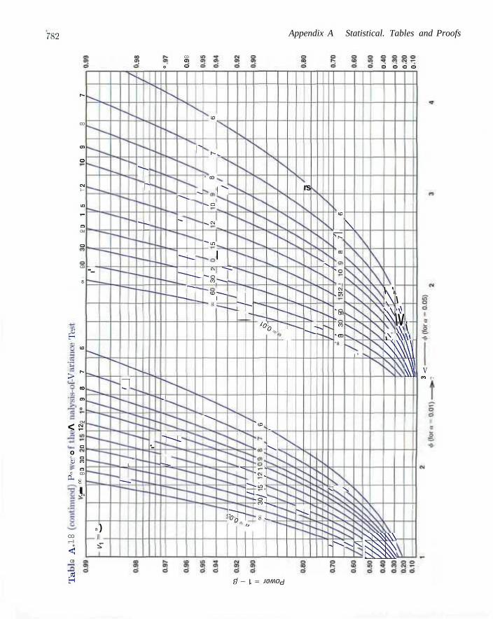
rs2 Appendix A Statistical. Tables and Proofs
| o
CD C l
O O O O O
E5
>
< s
o B
c OH
CO —I
< CD
0
t ^
CO
o i
o
CM 1—
i n
*-o CM
O
CD
8
CO
r~
CO
O l
o
CM
O
O CO
CO CD
S
|| -CM
..
a
1
)
i"
.J
T Y*
~_c
i • L
_____
.
j
P"
"*• " - * * c ,
*
•— ^
—•~- ^ :~~-]
^ ^ i
^•^^
__
CO
N ^
" CO
p* -S .O
s^CSI
^ m
| CN ""*•—.
"*-o cn^—.
C D — ^ .
1
^***»v
.
j ^ ______
i I J *
?"*
*°K
"co
r" * - C M ,
"**•«« J"_-"' r*--• 8 - ^
rs
__.
•Vj
8 - ^ .
Kt
rs.
^ > "-^s^l
^ ^
to
\ -
co
x o
£• stO
»o CM
CO
•o CO
" 8
sJ \
\
I s
^ N \ s.
\ \ N s \
\\N
\ \ \
\ v i >
\V w w
i
\ \ Nv.\
\ \ \ \ \ \ \ \ \ \ \ \ \
Hi
Vl
i
V CO r -
( 1 - 1 = J9M0d

Table A. 17 Table for the Signed-Rank Test 783
Table A. 17* Critical Values for the Signed-Rank Test
One-Sided a = 0.01 One-Sided a = 0.025 One-Sided a = 0.05 n Two-Sided a = 0.02 Two-Sided a = 0.05 Two-Sided a = 0.1
1 1 2 2 4 4 6 6 8 8 11
11 14 14 17 17 21 21 26 25 30
30 36 35 41 40 47 46 54 52 60
59 68 66 75 73 83 81 92 90 101
98 110 107 120 117 130 127 141 137 152
*Reproduced from F. Wilcoxon and R. A. Wilcox. Some Rapid Approximate Statistical Procedures, American Cyanamid Company, Pearl River, N.Y., 1964. by permission of the American Cyanamid Company.
5 6 7 8 9 10
11 12 13 14 15
16 17 18 19 20
21 22 23 24 25
26 27 28 29 30
0 2 3 5
7 10 13 16 20
24 28 33 38 43
49 56 62 69 77
85 93 102 111 120

784 Appendix A Statistical Tables and Proofs
Table A . 1 8 * Critical Values for the Wilcoxon Rank-Sum Test
One-Tai led Test at a = 0 .001 or T w o - T a i l e d Test at a = 0 .002 n2
m 6 7 8 9 10 11 12 13 14 15 16 17 18 19 20
1 2 3 4 5 0 0 6 0 1 2 7 8 9
10 11 12 13 14 15 16 17 18 19 20
2 3 5
1 2 3 5 7
0 1 3 5 6 8
10
0 2 4 6 8
10 12 15
0 2 4 7 9
12 14 17 20
1 3 5 8
11 14 17 20 23 26
1 3 0 9
12 15 19 22 25 29 32
1 4 7
10 14 17 21 24 28 32 36 40
2 5 8
11 15 19 23 27 31 35 39 43 48
0 2 5 9
13 17 21 25 29 34 38 43 47 52 57
0 3 6
10 14 18 23 27 32 37 42 46 51 56 61 66
0 3 7
11 15 20 25 29 34 40 45 50 55 60 66 71 77
0 3 7
12 16 21 26 32 37 42 48 54 59 65 70 76 82 88
One-Tailed Test at a = 0.01 or Two-Tailed Test at a = 0.02
n2
nx 5 6 7 8 9 10 11 12 13 14 15 16 17 18 19 20 1 2 3 4 0 5 1 6 7 8 9
10 11 12 13 14 15 16 17 18 19 20
0 1 1 2 3 3 4
6
0 2 4 6 8
10
1 3 5 7 9
11 14
1 3 6 8
11 13 16 19
I 4 7 9
12 15 18 22 25
2 5 8
11 14 17 21 24 28 31
0 2 5 9
12 16 20 23 27 31 35 39
0 2 6
10 13 17 22 26 30 34 38 43 47
0 3 7
11 15 19 24 28 33 37 42 47 51 56
0 3 7
12 16 21 26 31 36 41 46 51 56 61 66
0 4 8
13 18 23 28 33 38 44 49 55 60 66 71 77
0 4 9
14 19 24 30 36 41 47 53 59 65 70 76 82 88
1 4 9
15 20 26 32 38 44 50 56 63 69 75 82 88 94
101
1 5
10 16 22 28 34 40 47 53 60 67 73 80 87 93
100 107 114
*Based in part on Tables 1, 3, 5. and 7 of D. Auble, "Extended Tables for the Mann-Whitney Statistic," Bulletin of the Institute of Educational Research ai Indiana University, 1, No. 2, 1953, by permission of the director.

Table A.18 Table for the Rank-Sum Test 785
Table A.18 (continued) Critical Values for the Wilcoxon Rank-Sum Test One-Tailed Test at a = 0.025 or Two-Tailed Test at a = 0.05
n2
nx ~4 5 6 7 8 9" 10 i i 12" 13 14 15 16 17 18 19 20~ 1 2 3 4 I 5 6 7 8 9 10 11 12 13 14 15 16 17 18 19 20
0 1 ) 1 2
2 3 5
1 3 5 6 8
0 2 4 6 8 10 13
0 2 4 7 10 12 15 17
0 3 5 8 11 14 17 20 23
0 3 6 9 13 16 19 23 26 30
1 4 7 11 14 18 22 26 29 33 37
1 4 8 12 16 20 24 28 33 37 41 45
1 5 9 13 17 22 26 31 36 40 45 50 55
1 5 10 14 19 24 29 34 39 44 49 54 59 64
1 6 11 15 21 26 31 37 42 47 53 59 64 70 75
2 6 11 17 22 28 34 39 45 51 57 63 67 75 81 87
2 7 12 18 24 30 36 42 48 55 61 67 74 80 86 93 99
2 7 13 19 25 32 38 45 52 58 65 72 78 85 92 99 106 113
2 8 13 20 27 34 41 48 55 62 69 76 83 90 98 105 112 119 127
One-Tailed Test at a = 0.05 or Two-Tailed Test at a = 0.1
n_ 3 n2
4 5 6 7 8 9 10 11 12 13 14 15 16 17 18 19 20
1 2 0 3 0 0 1 4 5 6 7 8 9 10 11 12 13 14 15 16 17 18 19 20
1 2 4
0 2 3 5 7
0 2 4 6 8 11
1 3 5 8 10 13 15
1 4 6 9 12 15 18 21
1 4 7 11 14 17 20 24 27
1 5 8 12 16 19 23 27 31 34
2 5 9 13 17 21 26 30 34 38 42
2 6 10 15 19 24 28 33 37 42 47 51
3 7 11 16 21 26 31 36 41 46 51 56 61
3 7 12 18 23 28 33 39 44 50 55 61 66 72
3 8 14 19 25 30 36 42 48 54 60 65 71 77 83
3 9 15 20 26 33 39 45 51 57 64 70 77 83 89 96
4 9 16 22 28 35 41 48 55 61 68 75 82 88 95 102 109
0 4 10 17 23 30 37 44 51 58 65 72 80 87 94 101 109 116 123
0 4 11 18 25 32 39 47 54 62 69 77 84 92 100 107 115 123 130 138

786 Appendix A Statistical Tables and Proofs
Table A.19* P(V < v* when H0 is true) in the Runs Test
(nx,n2) (2,3) (2,4) 2,5
(2,6 (2,7) (2,8) (2,9) (2,10) (3,3) (3,4) (3,5) (3,6) t'i 7 i (3,8) (3,9) (3,10) m m (4,8) 4,9)
(4,10) (5,5) (5,6 (5,7 (5,8) (5,9) (5,10) 6,6)
(6,7 (6,8) (6,9) (6,10) (7,7) (7,8 (7,9) (7,10) (8,8) 8,9)
(8,10) (9,9) (9,10) (10,10)
2 0.200 0.133 0.095 0.071 0.056 0.044 0.036 0.030 0.100 0.057 0.036 0.024 0.017 0.012 0.009 0.007 0.029 0.016 0.010 0.006 0.004 0.003 0.002 0.008 0.004 0.003 0.002 0.001 0.001 0.002 0.001 0.001 0.000 0.000 0.001 0.000 0.000 0.000 0.000 0.000 0.000 0.000 0.000 0.000
3
0.500 0.400 0.333 0.286 0.250 0.222 0.200 0.182 0.300 0.200 0.143 0.107 0.083 0.067 0.055 0.045 0.114 0.071 0.048 0.033 0.024 0.018 0.014 0.040 0.024 0.015 0.010 0.007 0.005 0.013 0.008 0.005 0.003 0.002 0.004 0.002 0.001 0.001 0.001 0.001 0.000 0.000 0.000 0.000
4 0.900 0.800 0.714 0.643 0.583 0.533 0.491 0.455 0.700 0.543 0.429 0.345 0.283 0.236 0.200 0.171 0.371 0.262 0.190 0.142 0.109 0.085 0.068 0.167 0.110 0.076 0.054 0.039 0.029 0.067 0.043 0.028 0.019 0.013 0.025 0.015 0.010 0.006 0.009 0.005 0.003 0.003 0.002 0.001
5
1.000 1.000 1.000 1.000 1.000 1.000 1.000 1.000 0.900 0.800 0.714 0.643 0.583 0.533 0.491 0.455 0.629 0.500 0.405 0.333 0.279 0.236 0.203 0.357 0.262 0.197 0.152 0.119 0.095 0.175 0.121 0.086 0.063 0.047 0.078 0.051 0.035 0.024 0.032 0.020 0.013 0.012 0.008 0.004
V*
6
1.000 0.971 0.929 0.881 0.833 0.788 0.745 0.706 0.886 0.786 0.690 0.606 0.533 0.471 0.419 0.643 0.522 0.424 0.347 0.287 0.239 0.392 0.296 0.226 0.175 0.137 0.209 0.149 0.108 0.080 0.100 0.069 0.048 0.044 0.029 0.019
7
1.000 1.000 1.000 1.000 1.000 1.000 1.000 0.971 0.929 0.881 0.833 0.788 0.745 0.706 0.833 0.738 0-652 0.576 0.510 0.455 0.608 0.500 0.413 0.343 0.288 0.383 0.296 0.231 0.182 0.214 0.157 0.117 0.109 0.077 0.051
8
1.000 0.992 0.976 0.954 0.929 0.902 0.874 0.960 0.911 0.854 0.793 0.734 0.678 0.825 0.733 0.646 0.566 0.497 0.617 0.514 0.427 0.355 0.405 0.319 0.251 0.238 0.179 0.128
9
1.000 1.000 1.000 1.000 1.000 1.000 0.992 0.976 0.955 0.929 0.902 0.874 0.933 0.879 0.821 0.762 0.706 0.791 0.704 0.622 0.549 0.595 0.500 0.419 0.399 0.319 0.242
10
1.000 0.998 0.992 0.984 0.972 0.958 0.987 0.966 0.937 0.902 0.864 0.922 0.867 0.806 0.743 0.786 0.702 0.621 0.601 0.510 0.414
*Reproduced from C. Eisenhart and R. Swed, "Tables for Testing Randomness of Grouping in a Sequence of Alternatives," Ann. Math. Stat., 14, 1943, by permission of the editor.

Table A.19 Table for the Runs Test 787
Table A.19 (conti nued) P(V < v* when Ho is true) in the Runs Test
V*
( n i , n 2 ) 11 12 13 14 15 16 17 18 19 20
(2,3) (2,4) (2,5) (2,6) (2,7) (2,8) (2,9) (2,10) (3,3) (3,4) (3,5) (3,6) (3,7) (3,8) (3,9) (3,10)
(4,4) (4,5) (4,6) (4,7) (4,8) (4,9) (4,10) (5,5) (5,6) (5,7) (5,8) (5,9) (5,10) (6,6) (6,7) (6,8) (6,9) (6,10)
(7,7) (7,8) (7,9) (7,10) (8,8) (8,9) (8,10) (9,9) (9,10) (10,10)
1.000 1.000 1.000 1.000 1.000 0.998 0.992 0.984 0.972 0.958
0.975 0.949 0.916 0.879
0.900 0.843 0.782
0.762 0.681 0.586
1.000 0.999 0.998 0.994 0.990 0.996 0.988 0.975 0.957
0.968 0.939 0.903 0.891 0.834 0.758
1.000 1.000 1.000 1.000 0.999 0.998 0.994 0.990
0.991 0.980 0.964
0.956 0.923 0.872
1.000 1.000 0.999 0.998 0.999 0.996 0.990
0.988 0.974 0.949
1.000 1.000 1.000 1.000 0.999 0.998 0.997 0.992 0.981
1.000 1.000 1.000 1.000 0.999 0.996
1.000 1.000 1.000 1.000 0.999
1.000 1.000 1.000
1.000 1.000 1.000

788 Appendix A Statistical Tables and Proofs
Table A.20* Sample Size for Two-Sided Nonparametric Tolerance Limits
1-a 0.995 0.99 0.95 0.90 0.85
0.80 0.75 0.70 0.60 0.50
0.50
336 168 34 17 11
9 7 6 4 3
0.70
488 244 49 24 16
12 10 8 6 5
0.90
777 388 77 38 25
18 15 12 9 7
1 - 7 0.95
947 473 93 46 30
22 18 14 10 8
0.99
1,325 662 130 64 42
31 24 20 14 11
0.995
1,483 740 146 72 47
34 27 22 16 12
*Reproduced from Table A-25d of Wilfrid J. Dixon and Frank J. Massey, Jr. Introduction to Statistical Analysis, 3rd ed. McGraw-Hill, New York, 1969. Used with permission of McGraw-Hill Book Company.
Table A. 21* Sample Size for One-Sided Nonparametric Tolerance Limits
1 - a
0.995 0.99 0.95 0.90 0.85
0.80 0.75 0.70 0.60 0.50
0.50
139 69 14 7 5
4 3 2 2 1
0.70
241 120 24 12 8
6 5 4 3 2
1 - 7
0.95
598 299 59 29 19
14 11 9 6 5
0.99
919 459 90 44 29
21 7 13 10 7
0.995
1.379 688 135 66 43
31 25 20 14 10
*Reproduced from Table A-25e of Wilfrid J. Dixon and Frank J. Massey. Jr., Introduction to Statistical Analysis, 3rd ed. McGraw-Hill. New York, 1969. Used with permission of McGraw-Hill Book Company.

Table A.22 Table for Spearman's Rank Correlation Coefficients 789
Table A.22* Critical Values for Spearman's Rank Correlation Coefficients n
5 6 7 8 9
10
11 12 13 14 15
16 17 18 19 20
21 22 23 24 25
26 27 28 29 30
a = 0.05 0.900 0.829 0.714 0.643 0.600 0.564
0.523 0.497 0.475 0.457 0.441
0.425 0.412 0.399 0.388 0.377
0.368 0.359 0.351 0.343 0.336
0.329 0.323 0.317 0.311 0.305
a = 0.025
0.886 0.786 0.738 0.683 0.648
0.623 0.591 0.566 0.545 0.525
0.507 0.490 0.476 0.462 0.450
0.438 0.428 0.418 0.409 0.400
0.392 0.385 0.377 0.370 0.364
a = 0.01
0.943 0.893 0.833 0.783 0.745
0.736 0.703 0.673 0.646 0.623
0.601 0.582 0.564 0.549 0.534
0.521 0.508 0.496 0.485 0.475
0.465 0.456 0.448 0.440 0.432
a = 0.005
0.881 0.833 0.794
0.818 0.780 0.745 0.716 0.689
0.666 0.645 0.625 0.608 0.591
0.576 0.562 0.549 0.537 0.526
0.515 0.505 0.496 0.487 0.478
*Reproduced from E.G. Olds, "Distribution of Sums of Squares of Rank Differences for Small Samples," Ann. Math. Stat., 9. 1938, by permission of the editor.

790 Appendix A Statistical Tables and Proofs
O "3
t o
O 00
o
* CO CN
<
1
$ M
1 I L O
<tH
H->
CM
U
en - W
Is S ^ 0 o
Fac
t on
tr
O
for
lin
e
O + j
Fac
t C
en
I L
2 0
l I-H
U
£ ii 0
1
en H J
s I - )
L i
0 U
en « H
(H
fl) 4 J
fl I I I
u
en eu
a1
1 L i
a I u
I's
ti rSg o
tv co C O
O
C O L O 0 0
o
L O C D oo 0 0
o
0 0 C N r H
r H
C O O C O
C M
L O
C N
o
0 0 0 0
oo o tv o C D L O
o
C O C D C O
r H
C O t v C N
CN
C N 0 0 C N
C N
O
o 0 0 0 0
o
l O 0 0
o
C l L O o C N
0 0 0 0
c CN:
r H r-t
< N
c
N < C O 0 0
©
Oi Oi C N
o
C O C N C O
CM
C O O l
o c CM
o
0 0
0 0
o
C O
Oi C O
o
•>cf C O L O
CM
N < I N 0 0
Oi CN
o
CM Oi
C O I V o o
C O C O 0 0
o
0 0 Oi C O
co o
_* o C N
C O o 0 0
C O r H r H
C O 0 0
C O C O r ^
o
o C N 0 0
c CM r-^ l O co o I V
0 0
CM
r-i L O t -
Oi
r-l
C O r-< 0 0
0 0
o
0 0 o oo c
1 - -cc C O co
o o I V Oi
C N
I V o t v
C N C O C N
t v I V [ V
C O c N CM
o
1--o t -
o
Oi
CM C O
o
0 0 1 - -c C O
Oi C O C O
C N
N "
co L O CM
o
t v 0 0 t v
o
CM L O r H co o
C O I V H
C O
t v
C O C O
C O r H C O
l v H t v
oc CN
o
0 0 t v I V
o
o C O o co o
0 0 L O C N
C O
o r H CC
C O
C O
C O C D C O
I V
o C O o
o t v I V
o
oc Oi Oi C N
o
C O C O C O
C O
L O 0 0 L O
r -I V C O
CN t v C O
0 0 C N C O
o
C O C O t v
o
L O C O O l CM
o t v
o C O
C O C O L O
Oi Oi C O
C O L O C O
I V
CO
o
C O L O
o
o 0 0 0 0
o
C N
C O
N "
L O
CM
C O
cc
C O CO CO
o
o L O I V
o r ^ co oo C M
o
C N C O L O
C O
C O C N L O
o Tt<
CM CM
cc
oc [ V CO
o
I V
o t v
oo t v
< M
o
0 0 0 0 L O
C O
r-f r H L O
0 0 L O
N-
0 0 o CO
ci C O
o
O S CO I V
o t v i H t v ( M
c
C O
CO
CO C D
L O t v ^ H
Oi L O
C O
c o
_8f C O ( V
o
iv C N
O
Oi 0 0 C O
C O
0 C
o C 5
L O 0 0 L O
L O r-1
o Oi CN tv o t v
co C N
o
L O
C O
o [ V
*Cf r H LO
L O
L O C N
C
C N
o
1 ^ "* C O C N
o
0 0 I V
co
O l L O
C O r-H L O
C O C D L O
C O
o
o C M f -
c
oc r H co C N
CO
05 i—i 0 0
C O
0 0
0 0 C M L O
I V L O I O
CO
o C O r H I V
c
CM Oi l O C N
C
0 0 L O 0 0
CO
0 0 CO
C D C O L O
0 0
L O
L O
o CN —1 I V
o
1 -C D L O C M
O
L O C D O C
C O
C D CN
C D
L O
r-i
L O
r1
C D L O
O
0 0
1 ^
o
L O CM
O
C O C D
C O
o CM
C D L O L O
O O O O O O O O O O O O O O O O O O C 3 0 0 0 0
Is- 00 CO CD CO CO CO 00 CN LO CN O
O CN IO rH CO N » H C O H CD 00 00 Is- t -
CD CO 00 n< CN I V - r t r n O i t v O CD CO LO LO
CM T T 0 0 CO O LO CO —I O CD LO LO LO LO ^ r
N O I O L O U ) t— CD LO •n? CO ^ i ^ * ^ f ^ ^ i
CO CM CN CN
O 0 0 LO CD ^P CO r H 0 0 CO X O r H r H CN CM
H Ti l CN CO 0 0 CN LO 0 0 O CN CO CO CO M 1 M 1
CO CO CM N O •** CO 00 CD rn •*cH "*Ct* ^cfl TH LO
CO • * LO LO LO CN CO ^ LO CO LO LO LO LO LO
O O O O O O O O O O O O O O O O O O O O O O O O
M T f TJ I 0 0 CO 0 0 LO CO LO CN 0 0 CO CN r H O O
O CO CO t V r H r H CM CO r r 0 0 LO -_P CO CO CN O O O O O
CM CD O T * O LO CM r H CD 0 0 CN CN CM r H r H O O O O O
CC N CC O M CC LO T * -D" CO
CO CD - * CD LO CN — r - O O
O O O O O O O O O O
CD CN CO O t- CO rH O CD 00 IN rti IV 00 CD CD
o' o d o
CD -* 00 tv LO LO CN CN CO CD CO -* M rH r-i r-<
LO -tr O CO IV H Ol LO Ol CN LO LO CO CO tv CD CD CD CD CD O O O O O
tv CN CD CN LO 00 00 O) M N CN -H O O CD
•* C O N O C O LO IV CD rH CN t- S N 00 00 CD CD Ol Oi CD
LO LC Tf CM Ol CO '* LO CO CO 00 X- 00 00 00 CD CD CD CD CD
CO CN IV (N CO b- 00 00 Ol Ol 00 00 00 00 00 Oi Ol CD Ol Ol
O O O O O O O O O O O O O O O
N C O O N O CN 00 LO rH 00 Ol 00 00 00 t v
C O O O O O O O M N CO O CO C O C O r H O O O CO M1 CO r- O S N S CO CO CO CO CO <o CO
O O O O O O O O O O O O O O O O
O W O I N 00 CN CN t -00 O t v LO
CO Ol CO t v 00 00 rH IV CO O ™tf —Cf CO CO CO
LO CO CD LO CO 00 CO - * CO (M CM CM CN CN CM
CNI CO -H N O rH O Ol 00 00 CN CN r H r H —
CO I V CN ( V CO t - CO CD LO LO
r H r H O O O O O O O O O O O O O O O O O O O O O O
N W J I O e b - t o s O tH CN M r f W CO t v 00 O O
rH rH rH CN f l CN « rj< Ui CN ( N CN CN CN

Section A.25 Proof of Mean of the Hypergeometric Distribution 791
Table A.24 The Incomplete Gamma Function: F(x; a) = /<_f rh?,ya~le~y dy
a
X 1 2 3 4 5 6 7 8 9 10 1 0.6320 0.2640 0.0800 0.0190 0.0040 0.0010 0.0000 0.0000 0.0000 0.0000 2 0.8650 0.5940 0.3230 0.1430 0.0530 0.0170 0.0050 0.0010 0.0000 0.0000 3 0.9500 0.8010 0.5770 0.3530 0.1850 0.0840 0.0340 0.0120 0.0040 0.0010 4 0.9820 0.9080 0.7620 0.5670 0.3710 0.2150 0.1110 0.0510 0.0210 0.0080 5 0.9930 0.9600 0.8750 0.7350 0.5600 0.3840 0.2380 0.1330 0.0680 0.0320
6 0.9980 0.9830 0.9380 0.8490 0.7150 0.5540 0.3940 0.2560 0.1530 0.0840 7 0.9990 0.9930 0.9700 0.9180 0.8270 0.6990 0.5500 0.4010 0.2710 0.1700 8 1.0000 0.9970 0.9860 0.9580 0.9000 0.8090 0.6870 0.5470 0.4070 0.2830 9 0.9990 0.9940 0.9790 0.9450 0.8840 0.7930 0.6760 0.5440 0.4130
10 1.0000 0.9970 0.9900 0.9710 0.9330 0.8700 0.7800 0.6670 0.5420
11 0.9990 0.9950 0.9850 0.9620 0.9210 0.8570 0.7680 0.6590 12 1.0000 0.9980 0.9920 0.9800 0.9540 0.9110 0.8450 0.7580 13 0.9990 0.9960 0.9890 0.9740 0.9460 0.9000 0.8340 14 1.0000 0.9980 0.9940 0.9860 0.9680 0.9380 0.8910 15 0.9990 0.9970 0.9920 0.9820 0.9630 0.9300
A.25 Proof of Mean of the Hypergeometric Distribution To find the mean of the hypergeometric distribution, we write
n (k-l\(J\'-k\ — I S~* Vx-lKn-x/ - K 2L, (N\
x=l \n)
Since
(„^\)=C;1-,1-r
)) - ©-ao^-H-N/N-l n)\~ n \n-l)'
letting y = x — 1, we obtain
n-l (k-l\( N-k \
j/=0 in)
_ nk Y > ( y )j' n-i-y ) _ nk
y=0 \n-XJ
since the summation represents the total of all probabilities in a hypergeometric experiment when N — 1 items are selected at random from AT — 1. of which k — 1 are labeled success.

792 Appendix A Statistical Tables and Proofs
A.26 Proof of Mean and Variance of the Poisson Distribution Lot p = Xt.
e-^p* w-E-TF-E-Tf-rS^ni
1 = 0 1 = 1 1 = 1
e~''px-
3T-"i)i
Since the summation in the last term above is the total probability of a Poisson random variable with mean p which can be easily seen by letting y = x—l, it equals to 1. Therefore, E(X) = p.. To calculate the variance of X, note that
OO _ _ , . a, O O _ , , . y . _ 0
e V _ j r n C t'px * E\X(X - 1)] = 5>(:t: - lf-£- = p? Y, x=0 x=2 («2)«
Again, letting j / = I — 2, the summation in the last term above is the total probability of a Poisson random variable with mean p. Hence we obtain
cr2 = E(X2) - \E(X)}2 = E[X(X - 1)] + E(X) - [E(X)\2 = p2 + p. - p2 = p = Xt.
A.27 Proof that the Poisson Is a Limiting Form of the Binomial The binomial distribution can be written as
• • U " K « — r f ^ r ^ r ^ f 1 - ' 5 " -
njn - 1 ) - • • (n - x +1) x px(l-p)n-*.
Substituting p = p/n,
b(x;n,p) = i(n - ! ) • • • (n - x + 1) /p
($(»-£) -KhO-^so-i.H-r-
As n —* oo while x and p remain constants,
lim 1 ( 1 - -n—»oo \ 71
and from the definition of e.
1 -. X ' - l
= 1, lim {l-'-YX = l. n—»oc \ nJ
lim f l - - ) = lim TI—.oc \ n ' n—»c
-i -n/n'
1 + ( - " ) / r
= e
Hence, under the given limiting conditions,
bix;n,p)->~f-, 1 = 0,1,2,.... :r:

Section A.28 Proof of Mean and. Variance of the Gamma Distribution 793
A.28 Proof of Mean and Variance of the Gamma Distribution Tei find the mean anel variance of the1 gamma distribution, we first calculate
E( /•oo ,«rivr/n, I i.] roc va+k-l„-x/p
A ) d»r(a)j0 ' CU ll»T(a) ./,-, P^r(a + k)aj"
for k = 0,1,2 Since the integrand in the1 last term above- is a gamma density function with parameters a + k and ii, it equals 1. Therefore,
r(o)
Using the recursion formula of the gamma function from page 194, we obtain
T(a'T-l) __ , 2 , j 2 r ( f v + 2 ) 2 ,.2 . , \ . ,o\2 ,o2 // = / j — — — — = dtp and a = £/(A ) — p = ,o ——— p = p a(a + I) — (ap) = ap.

Appendix B
Answers to Odd-Numbered Non-Review Exercises
Chapter 1
1.1 (a) Sample size = 15
(b) Sample mean = 3.787
(c) Sample median = 3.6
(e) *tr(20) = 3- ( i 7 8
1.3 (b) Yes, aging process reduced the tensile strength.
(c) xAglng = 209.90. xKo _.gjns = 222.10
(d) XAging = 210.00, KNO aging = 221.50. The means ane] medians are similar for e:ach group.
1.5 (b) Control: x = 5.60, x = 5.00, :i; t l. ( lu) = 5.13. Treatment: if: = 7.60, z = 4.50, s ti(l0) =
5.63.
(c) The extreme value of 37 in the treatment group plays a strong leverage role for the mean calculation.
1.7 Sample variance = 0.943 Sample standard deviation = 0.971
1.9 No aging: sample variance = 23.62, sample standard deviation = 4.86. Aging: sample variance = 42.12, sample standard deviation = 0.49.
1.11 Control: sample variance = 69.38, sample standard deviation = 8.33. Treatment: sample variance = 128.04. sample standard deviation = 11.32.
1.13 (a) Mean = 124.3, median = 120;
(b) 175 is an extreme observation.
1.15 Yes, P-value = 0.03125; probability of obtaining HHHHII with a fair coin.
1.17 Nonsmokers (a) 30.32, (b) 7.13; Smokers (a.) 43.70, (b) 16.93. (d) Smokers appear to take longer time to fall asleep. For smokers the time to fall asleep is more: variable.
1.19
1.21
Stem.
0
2 3 4 5 6
Leaf 22233457 023558 035 03 057 0569 0005
Frequency 8 6 3 2 3 4 4
(b) Class Class Re l . In te rva l Midpo in t Fi-eq. Freq. 0.0-0.9 1.0-1.9 2.0-2.9 3.0-3.9 4.0-4.9 5.0-5.0 0.0-6.9
0.45 1.45 2.45 3.45 4.45 5.45 6.45
8 6 3 2 3 4 4
0.267 0.200 0.100 0.067 0.100 0.133 0.133
(c) Sample mean = 2.7967 Sample range = 6.3 Sample! standard deviation 2.2273
(a) Sample mean = 1.7743 Sample median = 1.77
(b) Sample standard deviation = 0.3905.

796 Appendix B Answers to Odd-Numbered Non-Review Exercises
1.23 (b) xi99o = 160.15, a-1980 = 395.10.
(c) The mean emissions dropped between 1980 and 1990, the variability also decreased because there were no longer extremely large emissions.
1.25 (a) Sample mean = 33.31
(b) Sample median = 26.35
(d) x t r ( 1 0 ) = 30.97
Chapter 2
2.1 (a) 5= {8,16,24,32,40,48}
(b) S = { - 5 , 1 }
(c) S = {T, UT, HHT, HHH}
(d) S = {Africa, Antarctica. Asia, Australia, Europe, North America, South America}
(e) S = <p
2.3 A = C
2.5 S ={1HH. \HT, ITH, ITT, 2H, 2T, 'AHH, 3HT, 3777, 3TT. 4H. AT, bHH. 5HT, 5TH, oTT, &H, 6T}
2.7 Sx ={MMMM,MMMF,MMFM.MFMM, FMMM. MMFF. MFMF. MFFM. FMFM, FFMM, FMMF, MFFF. FMFF, FFMF, FFFM,FFFF}; S2 ={0 ,1 ,2 ,3 ,4}
2.9 (a) A = {1HH, 1HT, ITH, ITT. 2H, 2T}
(b) B = { i rT ,3TT ,5TT}
(c) A ={3HH,3HT.3TH.3TT,4H,4T, hHH, hHT, 5TH, oTT, 6H, 6T}
(d) A n B = {3TT, 5TT}
(e) AUB={1HH. IHT,1TH, ITT.2H.2T, 3TT, 5TT}
2.11 (a) S={MxM2.MiFx,MxF2,M2Mx,M2Fx, M2 F2, F, Mx, Fi M2 ,FxF2, F2 Mv, F2 M2, F2Fx)
(b) A = {M\Mo,MyFi,MiF2,M2Mx,M2F], M2F2]
(c) B = {MxF1,MiF2,M2FJ.M2F2.F\Mi. FxM2,F2Mi,F2M2)
(d) C={FxF2,F2Fi}
(e) A O B = {MiFi,MxF2, M2Fi,M2F2}
(f) A U C={MiM2, MxFi, 1V/1F2, M2Mx, M2FuM2F2,FxF2,F2Fx}
2.15 (a) {nitrogen, potassium, uranium, oxygen}
(b) {copper, sodium, zinc, oxygen}
(c) {copper, sodium, nitrogen, potassium, uranium, zinc}
(d) {copper, uranium, zinc}
(e) $
(f) {oxygen}
2.19 (a) The family will experience mechanical problems but will receive no ticket for traffic violation and will not arrive at a campsite that has no vacancies.
(b) The family will receive a traffic ticket and arrive at a campsite that has no vacancies but will not experience mechanical problems.
(c) The family will experience mechanical problems and will arrive at a campsite that has no vacancies.
(d) The family will receive a traffic ticket but will not arrive at a campsite that has no vacancies.
(e) The family will not experience mechanical problems.
2.2]
2.23
2.25
2.27
2.29
2.31
2.33
2.35
2.37
2.39
2.41
2.43
2.45
2.47
2.49
18
156
20
48
210
(a) 1024;
72
362,880
2,880
(b) 243
(a) 40,320; (b) 336
360
24
3,360
7,920
56

Chapter 3 797
2.51 (a) Sum of the probabilities exceeds 1.
(b) Sum of the probabilities is less than 1.
(c) A negative probability.
(d) Probability of both a heart and a black card is zero.
2.53 S = {$10, $25, $100}: P(10) = ^ ; P(25) = fjj,
Pim = Tab 5u 2.55 (a) 0.3; (b) 0.2
2.57 (a) 5/26; (b) 9/26; (c) 19/26
2.59 10/117
2.61 95/663
2.63 (a) 94/54,145; (b) 143/39,984
2.65 (a) 22/25; (b) 3/25; (c) 17/50
2.67 (a) 0.32; (b) 0.68; (c) office or den
2.69 (a) 0.8; (b) 0.45; (c) 0.55
2.71 (a) 0.31; (b) 0.93; (c) 0.31
2.73 (a) 0.009; (b) 0.999: (c) 0.01
2.75 (a) 0.048; (b) $50,000; (c) 812,500
2.77 (a) The probability that a convict who pushed dope also committed armed robbery.
(b) The probability that a convict who committed armed robbery did not push dope.
(c) The probability that a convict who did not push dope also did not commit armed robbery.
2.79 (a) 14/39; (b) 95/112
2.81 (a) 5/34; (b) 3/8
2.83 (a) 0.018; (b) 0.614; (c) 0.166; (d) 0.479
2.85 (a) 0.35; (b) 0.875; (c) 0.55
2.87 (a) 9/28; (b) 3/4; (c) 0.91
2.89 0.27
2.91 5/8
2.93 (a) 0.0016; (b) 0.9984.
2.95 (a) 1/5; (b) 4/15; (c) 3/5.
2.97 (a) 91/323; (b) 91/323.
2.99 (a) 0.75112 (b) 0.2045.
2.101 0.0960
2.103 0.40625
2.105 0.1124
2.107 (a) 0.045; (b) 0.564; (c) 0.630; (d) 0.1064
Chapter 3
3.1 Discrete; continuous; continuous; discrete; discrete; continuous.
3 3 Sample Space
HHH HHT HTH THH HTT THT TTH TTT
3
—1 - 1 - 1 - 3
3.5 (a) 1/30; (b) 1/10
3.7 (a) 0.68; (b) 0.375
3.9 (b) 19/80
3.11
3.13
fix) 0
F(x) = <
(0, f o r x < 0 , 0.41, for 0 < x< 1 0.78, for 1 < a: < 2 0.94, for 2 < x < 3 0.99, for 3 < x < 4, 1, for x > 4
3.15 0. 2 7> 6 7> 1,
for x < 0, for 0 < :r < 1, for 1 < a: < 2, for x > 2
Fix) = i
(a) 4/7; (b) 5/7
3.17 (b) 1/4; (c) 0.3
3.19 F(x) = (x- l ) /2 , for 0 < x < 3; 1/4
3.21 (a) 3/2; (b) F(x) = xAl2, for 0 < x < 1; 0.3004

798 Appendix B Answers to Odd-Numbered Non-Review Exercises
3.23
F(w) = .
3.25
fO, f o r u i < - 3 , for — 3 < w < —1, for - 1 < w < 1, for 1 < in < 3,
_1, for w > 3 (a) 20/27; (b) 2/3
20 25 30
3.53 (a) l
27' 7
37 ' 19 27'
3.27
P(T = t)
(a) F(x) =
i
0,
3 1
a: < 0 .
1 -exp(-a- /2000) , x > 0. (b) 0.6065; (c) 0.6321
3.29 (b) F(x)
0,
3.31
3.33
3.35
3.37
3.39
1 - x ~ a
(a) 0.2231; (b) 0.2212
x < 1, x> 1.
(c) 0.0156
(a) fc = 280; (b) 0.3633: (c) 0.0563
(a) 0.1528; (b) 0.0446
(a) 1/36; (b) 1/15
(a) x
ffay) 0 1 2
(b) 1/2
0 1 "Ti 3 _
2 I
¥ ¥ 7TJ 70
^_J_~
1 f 70"
7_r~
7l>
3.41 (a) 1/16; (b) g(x) = 12.x-(l - a;)2, for 0 < :r < 1; (c) 1/4
3.43 (a) 3/64; (b,
3.45 0.6534
3.47 (a) Depende
3.49 (a) x
gix) (b) y
h(y) (c) 0.5714
3.51 (a)
1/2
nt; (b)
1 0.10
1 0.20
ffay)
y
(b) 11/12
0 1 2
1/3
2 0.35
2 0.50
0
f 315
3 0.55
3 0.30
X
1 2 H 1 "
I o 0 0
/(«>0>> 0
y i 2 3
(b) 42/55
3.55 5/8
3.57 Independent
3.59 (a) 3; (b) 21/512
3.61 Dependent
Chapter 4
4.1 0
4.3 25 cents
4.5 0.88
4.7 $500
4.9 S1.23
4.11 $6,900
4.13 (ln4)/7r
4.15 100 hours
4.17 209
4.19 $1,855
4.21 $833.33
4.23 (a) 35.2; (b) px =
4.25 2
4.27 2,000 hours
4.29 (b) 3/2
4.31 (a) 1/6; (b) (5/6)5
4.33 $5,250,000
4.35 0.74
0 1 2 1 6 6
¥ I f I f f ? 55 55 u
55 0 0
3.20, pY = 3.00
4.37 1/18; in actual profit the variance is
4.39 1/6
3 1
55 0 0 0
TS(5000)2

Chapter 5 799
4.41 118.9
4.43 pY = 10; oY = 144.
4.45 aXY = 0.005
4.47 -0.0062
4,49 o2x = 0.8456; <x.v = 0.9196
4.51 10.33: 6.66
4.53 80 cents
4.55 209
4.57 //. = 7/2; o2 = 15/4
4.59 3/14
4.61 0.03125
4.63 0.9340
4.65 52
4.67 (a) At most 4/9; (b) at least 5/9; (c) at least 21/25; (d) 10.
4.69 (a) 7; (b) 0; (c) 12.25
4.71 46/63
4.73 (a) 2.5: 2.08
4.75 (a) E(X) = E(Y) = 1/3 and Var(X) = Var(Y) = 4/9; (b) E(Z) = 2/3 and Var(Z) = 8/9
4.77 (a) 4; (b) 32; 16
4.79 By direct calculation, ^(e*") = 1,884.32 Using the second order adjustment approximation, E(e ) % 1. 883.38. which is very close to the true value.
Chapter 5
5.1 3/10
5.3 p. = 5.5; a 8.25
5.5 (a) 0.0480; (b) 0.2375; (c) P(X = 5\p = 0.3) 0.1789, P = 0.3 is reasonable.
5.7 (a) 0.0474: (b) 0.0171
5.9 (a) 0.7073; (b) 0.4613; (c) 0.1484
5.11 0.1240
5.13 0.8369
5.15 (a) 0.0778; (b) 0.3370; (c) 0.0870
5.17 p±2a = 3.5 ± 2.05
5.19 f(xux2,x-j) = (x. _* _i:.i)0.35X!0.05:l'20.60T:)
5.21 0.0095
5.23 0.0077
5.25 0.8070
5.27 (a) 0.2852; (b) 0.9887: (c) 0.6083
5.29 (a) 0.3246; (b) 0.4496
5.31 5/14
5.33 h(x;6,3.4) = ^ k " , for x = 1,2,3;
P(2 < X < 3) = 4J/5
5.35 0.9517
5.37 (a) 0.6815; (b) 0.1153
5.39 3.25: from 0.52 to 5.98
5.41 0.9453
5.43 0.6077
5.45 (a) 4/33; (b) 8/165
5.47 0.2315
5.49 (a) 0.3991; (b) 0.1316
5.51 0.0515
5.53 (a) 0.3840; (b) 0.0067
5.55 63/64
5.57 (a) 0.0630; (b) 0.9730
5.59 (a) 0.1429; (b) 0.1353
5.61 (a) 0.1638; (b) 0.032
5.63 (a) 0.3840; (b) 0.1395; (c) 0.0553
5.65 0.2657
5.67 (a) p = 4;a2= 4; (b) From 0 to 8.
5.69 (a) 0.2650; (b) 0.9596
5.71 (a) 0.8243; (b) 14

800
5.73 4
5.75 5.53 x 1 0 - 4 ; p = 7.5
5.77 (a) 0.0137; (b) 0.0830
5.79 0.4686
Chapter 6
6.1
Appendix B Answers to Odd-Numbered Non-Review Exercises
6.47 (a) yfiT/2 = 1.2533; (b) e - 2
6.49 e~4 = 0.0183
6.51 (a) p = ad = 50; (b) er2 = ap2 = 500; a = v/500; (c) 0.815
6.53 (a) 0.1889; (b) 0.0357
6.55 Mean=e6 . variance=e12(e4 - 1)
6.57 ( a ) e - 1 0 ; (b) 3 = 0.10
6.3
6.5
6.7
6.9
6.11
6.13 6.24 years
6.15
6.17
6.19 26
6.21
6.23
6.25
6.27
6.29
6.33
6.35
6.37
6.39 2.8c
6.43
a) 0.9236; (b) 0.8133; (c) 0.2424; d) 0.0823; (e) 0.0250; (f) 0.6435
a) -1.72; (b) 0.54; (c) 1.28
a) 0.1151; (b) 16.1; (c) 20.275; (cl) 0.5403
a) 0.8980; (b) 0.0287: (c) 0.6080
a) 0.0548; (b) 0.4514; (c) 23; d) 189.95 milliliters
a) 0.0571: (b) 99.11%; (c) 0.3974: d) 27.952 minutes; (e) 0.0092
a) 51%; (b) 818.37
a) 0.0401; (b) 0.0244
a) 0.6; (b) 0.7; (c) 0.5
a) 0.8006: (b) 0.7803
a) 0.3085: (b) 0.0197
a) 0.9514; (b) 0.0668
a) 0.1171; (b) 0.2049
6.31 0.1357
a) 0.0778; (b) 0.0571; (c) 0.6811
a) 0.8749; (b) 0.0059
a) 0.0228; (b) 0.3974
- 1 . 8 3.4e~2-4 = 0.1545
a) p = 6; a2 = 18; b) from 0 to 14.485 million litters.
6
Chapter 7
7.1 g(y) = 1/3; for y = 1,3, 5
fl(?/l,2/2)= Ln+«i,n-V2t2 yi
for yx = 0 , 1 , 2 ; y2 = -2, - 1 , 0 , 1 , 2 ; V2 <yi',Vl +2/2 = 0,2,4
7.7 Gamma distribution with a = 3/2 and 0 = m/26
7.9 (a) g(y) = 32/y3, for y > 4; (b) 1/4
7.11 h(z) = 2(1 - z), for 0 < 2 < 1
7.13 h(w) = 6 + 6ui - 12w1 / 2 , for 0 < w< 1
7.
6-45 £ 0(1 - e-^4)x(er''i'4)G-x = 0.3968 x=4
7.19 Both equal p
7.23 (a) Gamma(2,l); (b) Uniform(0,l)
Chapter 8
8.1 (a) Responses of all people in Richmond who have a telephone;
(b) Outcomes for a large or infinite number of tosses of a coin;
(c) Length of life of such tennis shoes when worn on the professional tour;
(d) All possible time intervals for this lawyer to drive from her home to her office.

Chapter 9 801
8.3
8.5
8.7
8.9
8.11
8.13
8.15
8.17
8.19
8.21
8.23
8.25
8.29
8.33
8.35
8.37
8.39
8.41
8.43
8.47
8.49
8.51
8.53
8.55
a) x = 2.4; (b) x = 2:(c)m = 3
a) x = 3.2 seconds; (b) x = 3.1 seconds
a) 53.75; (b) 75 and 100
a) Range is 10: (b) s = 3.307
a) 2.971; (b) 2.971
; = 0.585
a) 45.9; (b) 5.1
0.3159
a) Reduced from 0.49 to 0.16; b) Increased from 0.04 to 0.64
Yes.
a) p = 5.3; er2 = 0.81; b) px = 5.3; o\ = 0.0225:
c) 0.9082
a) 0.6898; (b) 7.35
0.5596
a) 0.1977; (b) No
a) 1/2; (b) 0.3085
P(X < 7751// = 760) = 0.9332
a) 27.488; (b) 18.475; (c) 36.415
a) 0.297; (b) 32.852; (c) 46.928
a) 0.05; (b) 0.94
a) 0.975; (b) 0.10; (c) 0.875; (d) 0.99
a) 2.500; (b) 1.319; (c) 1.714
No; p > 20
a) 2.71; (b) 3.51; (c) 2.92; d) 0.47; (e) 0.34
The .F-ratio is 1.44. The variances are not significantly different.
Chapter 9
9.5 0.3097 < p < 0.3103
9.7 (a) 22, 496 < p < 24,504; (b) error < 1004
9.9 35
9.11 56
9.13 0.978 <p< 1.033
9.15 47.722 < p < 49.278
9.17 323.946 to 326.154
9.19 11,426 to 35,574
9.23 The variance of S'2 is smaller.
9.25 (6.05,16.55)
9.27 (1.6358, 5.9376)
9.29 Upper prediction bound: 9.42; Upper tolerance limit: 11.72
9.33 Yes, the value of 6.9 is outside of the prediction interval.
9.35 2.9 < px - p2 < 7.1
9.37 2.80 <pi-p2< 3.40
9.39 1.5 < pi - p2 < 12.5
9.41 0.70 < pi - p2 < 3.30
9.43 -6 ,536 < px - p2 < 2,936
9.45 (-0.74,6.30)
9.47 (-6.92,36.70)
9.49 0.54652 < pB - pA < 1.69348
9.51 (a) 0.498 < p < 0.642; (b) error < 0.072
9.53 0.194 < p < 0.262
9.55 (a) 0.739 < p < 0.961; (b) no
9.57 (a) 0.644 < p < 0.690; (b) error < 0.023
9.59 2,576
9.61 160
9.63 16,577
9.65 -0.0136 < pF - pM < 0.0636
9.67 0.0011 < p, - p 2 < 0.0869
9.69 (-0.0849,0.0013); not significantly different.
9.71 0.293 < er2 < 6.736; valid claim
9.73 3.472 < er2 < 12.804

802 Appendix B Answers to Odd-Numbered Non-Review Exercises
9.75 9.27 < a < 34.16
9.77 0.549 < <TI/(T2 < 2.690
9.79 0.016 < a\/a\ < 0.454; no
9.81 1 fl xt j = i
9.83 (a) L(x\,x2 .r„) =
(2
(b) p=-\ E In a',:
i A i / i \ / £ ( l n , , - " ) ' / J * '
; = i
- 2 _ 1 ^ 1=1
h\xi- -\ £ hi-Tj
9.85 a:lnp-|- (1 — s)lii(l - p ) . Set the derivative with respect to p = 0; p = x = 1.0
Chapter 10
10.1 (a) Conclude that fewer than 30% of the public are allergic to some cheese products when, in fact, 30% or more are allergic.
(b) Conclude that at least 30% of the public are allergic to some cheese products when, in fact, fewer than 30% are allergic.
10.3 (a) The firm is not guilty;
(b) the firm is guilty.
10.5 (a) 0.1286;
(b) 3 = 0.0901; 3 = 0.0708.
(c) The probability of a type I error is somewhat, large.
10.7 (a) 0.0559;
(b) 0 = 0.0017; 3 = 0.00968; 3 = 0.5557
10.9 (a) a = 0.0032; (b) 3 = 0.0062
10.11 (a) a = 0.1357; (b) 3 = 0.2578
10.13 a = 0.0094; ,3 = 0.0122
10.15 (a) Q = 0.0718; (b) 3 = 0.1151
10.17 (a) Q = 0.0384; (b) 3 = 0.5; 3 = 0.2776
10.19 z= -1.64; P-valuc=0.10
10.21 2 = -2.76; yes, p < 40 months; P-value=0.0029
10.23 z = 8.97; yes, //. > 20,000 kilometers; P-value< 0.001
10.25 t = 0.77; fail to reject Ho-
10.27 t = 12.72; P-value < 0.0005; reject H0.
10.29 t = -1.98; Reject //(.; P-value = 0.0312
10.31 z = —2.60; conclude p/, — PQ < 12 kilograms.
10.33 t = 1.50; no sufficient evidence to conclude that the increase in substrate concentration would cause an increase in the mean velocity by more than 0.5 micromolc per 30 minutes.
10.35 t = 0.70; no sufficient evidence to support that the serum is effective.
10.37 t = 2.55; reject HQ: p\ — u2 > 4 kilometers.
10.39 t = 0.22; fail to reject HQ.
10.41 t = 2.76; reject H0-
10.43 t = 2.48; P-value < 0.02; reject Ho
ld.45 t = —2.53; reject Ho', the claim is valid.
10.47 n = 6
10.49 78.28 « 79 due to round up.
10.51 5
10.53 (a) H0: M h o t - .V/COM = 0, Hi: 1 1 / ^ - itfcoui 9* 0;
(b) paired t, t = 0.99; P-value > 0.30; fail to reject Ho.
10.55 P-value = 0.4044 (with a one-tailed test); the claim is not refuted.
10.57 P-value = 0.0207; yes, the coin is not balanced.
10.59 z = —5.06 and P-value RS 0; conclude that le ss than 1/5 of the homes are heated by oil.
10.61 z = 1.44; fail to reject Ha.
10.63 z = 2.36 with P-value = 0.0182; yes, the difference is significant.
10.65 z = 1.10 with P-valuc = 0.1357; we do not have sufficient evidence to conclude that breast cancer is more prevalent in the urban community.

Chapter 11 803
10.67 x 2 = 18-13 with P-value = 0.0676 (from com- 11.7 (b) y = 343.706 + 3.221a;; puter output): do not reject HQ: a2 = 0.03. (c) y = $ 4 5 6 a t advertising casts being $35
10.69 x 2 = 63.75 with P-value = 0.8998 (from com- 11.9 (a) y = 153.175 - 6.324a;; puter output); do not reject H0. ( b ) - = m ^ x = 4g u n j t s
10.71 x2 = 42-37 with P-value = 0.0117 (from com- 1 U 1 (b) y = -1847.633 + 3.653a: puter output); machine is out of control.
11.13 (b) y = 31.709 + 0.353a; 10.73 / = 1.33 with P-value = 0.3095 (from computer
output); fail to reject H0: ax = a2. 11.17 (a) s2 = 176.4;
10.75 / = 0.086 with P-value = 0.0328 (from com- (b) ' = 2 '04= f a i l t o r c J e c t H»' $ = °-puter output); reject HQ: ax = o2 at level greater n , a < \ 2 _ n An
than 0.0328. i l - i J W S ~ U 4 U ;
(b) 4.324 < Q < 8.503; 10.77 / = 19.67 with P-valuc = 0.0008 (from com- , , o 446 < 3 < 3 172
puter output); reject Ho'. a\ = a2. , 11.21 (a) s2 = 6.626:
10.79 x = 4-47; there is no sufficient evidence to claim that the coin is unbalanced. (b) 2.684 < a < 8.968;
10.81 x - 1 0-1 4 ; reJect H0, the ratio is not 5:2:2:1. (c) 0.498 < 0 < 0.637
11.23 t = -2.24; reject H0: 0 < 6 10.83 x2 = 2-33; do not reject H0: binomial distribu
tion. 11.25 (a) 24.438 < pY\24.5 < 27.106;
10.85 x2 = 3.125; do not reject H0: geometric distri- (b) 2 1 ' 8 8 < W> < 2 9 ' 6 6
b u t i o n ' 11.27 7.81 < /lyiLo < 10.81
10.89 x2 = 5.19; do not reject HQ: normal distribution. . . 9„ , , . , . „ . „
10.91 x = 5.47; do not reject Ho. (b) no, (the 95% confidence interval on mean mpg is (27.95,29.60));
10.93 x — 124.59; yes, occurrence of these tvpes of . . ., .,, crime is dependent on the city district. " ^ m , , e s P e r S a l l o n wl11 l l k e l>" e x c e e d 1 8
10.95 x 2 = 31.17 with P-value < 0.0001; attitudes are 1 1 3 3 ^ * = 3Al56x
not homogeneous. *
10.97 x 2 = 5-92 with P-value = 0.4332: do not reject 1 L 3 5 (a) b = '"«, j '•• HQ. , 5 X '
10.99 x = 1'84: do not reject HQ.
Chapter 11
(b) ?) = 2.003a:
J2 (^li-S'l)3'2i 11.37 E(B)=0 + ~p-=h
11.39 (a) a = 10.812, b = -0.3437;
11.1 (a) a = 64.529, b = 0.561; (b) t = 0 .43 ; the regression is linear.
(b) 0 = 81.4
11.3 (a) j / = 6.4136 + 1.8091a:;
11.41 / = 1.12; the regression is linear.
11.43 / = 1.71 and P-value = 0.2517; the regression is (b) y = 9.580 at temperature 1.75 linear.
11.5 (a) 0 = 5.8254 +0.5676a;; 11.45 (a) P = -11 .3251 - 0.0449X;
(c) y = 34.205 at 50° C (b) yes;

804 Appendix B Answers to Odd-Numbered Non-Review Exercises
(c) R2 = 0.9355;
(d) yes
11.47 (b) N = -175.9025 + 0.0902V; R2 = 0.3322.
11.49 r = 0.240
11.53 (a) r = 0.392;
(b) t = 2.04; fail to reject HQ: p = 0; however, the P-value = 0.053 is marginal.
Chapter 12
12.1 (a) y = 27.547 -1- 0.922a;. + 0.284x2;
(b) y = 84 at x_ = 64 and x2 = 4.
12.3 y = 0.5800 + 2.7122z. + 2.0497x2.
12.5 (a) y = 56.4633 + 0.1525.x- 0.00008a:2;
(b) y = 86.7% when temperature is at 225°C.
12.7 y = 141.6118 - 0.2819a; + 0.0003a:2.
12.9 (a) y = -102.7132 + 0.6054x. + 8.9236.r2 + 1.4374a;3 + 0.0136.T4:
(b) t} = 287.6.
12.11 0 = 3.3205 + 0.4210a:. - 0.2958x2 + 0.0164x3 + 0.1247x4.
12.13 0 = -6.5122 + 1.9994x1 - 3.6751x2 + 2.5245x3 + 5.1581x4 + 14.4012x5.
12.15 (a) 0 = 350.9943 - 1.2720x. - 0.1539x2:
(b) 0 = 140.9
12.17 0.1651
12.19 242.72
12.21 (a) a%3 = 28.0955; (b) aB, B 2 = -0.0096
12.23 29.93 < PY\XQ.& < 31.97
12.25 t = 2.86; reject H0 and in favor of 32 > 0.
12.27 t = 3.524 with P-value = 0.01; reject HQ and in favor of 0i > 2.
12.29 (a) t = -1.09 with P-value = 0.3562;
(b) t = -1.72 with P-value = 0.1841:
(c) Yes; no sufficient evidence to show that xi and x2 are significant.
12.31 R2 = 0.9997
12.33 / = 5.106 with P-value = 0.0303; the regression is not significant at level 0.01.
12.35
12.37
12.39
12.41
12.43
12.45
12.47
12.49
12.51
12.53
/ = 34.90 with P-value = 0.0002; reject HQ and conclude 0\ > 0.
/ = 10.18 with P-value < 0.01; xi and x2 are significant in the presence of 13 and X4.
The two-variable model is better.
First model: R2^ = 92.7%, CV = 9.0385;
Second model: R2^ = 98.1%, CV = 4.6287; The partial /—test shows P-value = 0.0002; model 2 is better.
Using x2 alone is not much different from using xi and x2 together since the R^yS are 0.7696 versus 0.7591.
(a) mpg = 5.9593 - 0.00003773 odometer + 0.3374 octane - 12.6266«i - 12.9846^;
(b) sedan;
(c) they are not significantly different.
(b) 0 = 4.690 seconds;
(c) 4.450 < /iy|{i80,260} < 4.930
0 = 2.1833 + 0.9576x2 + 3.3253x3
(a) 0 = -587.211 + 428.433x;
(b) 0 = 1180 - 191.691x + 35.20945x2;
(c) quadratic model
a2Bl = 20,588; &2
Bll = 62.6502; o-B,,B„ = -1103.5
12.55 (a) Intercept model is the best.
12.57 (a) 0 = 3.1368 + 0.6444xi - 0.0104x2 + 0.5046x3 - 0.1197x4 - 2.4618x5 + 1.5044x6;
(b) 0 = 4.6563 + 0.5133x3 - 0.1242x4;
(d) 0 = 4.6563+ 0.5133x3-0.1242x4;
(e) two observations have large .R-student values and should be checked.
12.59 (a) 0 = 125.8655 + 7.7586xi + 0.0943x2 -0.0092xix2;
(b) the model with x 2 alone is the best.

Chapter 13 805
Chapter 13
13.3 / = 0.31; no sufficient evidence to support that there are differences among the 6 machines.
13.5 / = 14.52: yes, the difference is significant
13.7 / = 2.25; no sufficient evidence to support that the different concentrations of MgNH4P04 significantly affect the attained height of chrysanthemums.
13.9 / = 8.38; the average specific activities differ significantly.
13.11 (a) / = 14.28; reject H0;
(b) / = 23.23; reject HQ:
(c) / = 2.48; fail to reject H0.
13.13 (a) / = 13.50; treatment means differ;
(b) / ( l vs. 2)=29.35: significant; / ( 3 vs. 4)=3.59; not significant
13.15 X3 Xi x 4 •1:2
56.52 59.66 61.12 61.96
13.17 (a) / = 9.01; yes, significant;
(b) Substrate Modified Removal
Depletion Hess Kicknet Surber Kicknet
13.35 / = 0.58; not significant
13.39 / = 5.03; grades are affected by different professors.
13.41 p < 0.0001; / = 122.37; the amount of dye has an effect on the color of the fabric.
13.43 (a) / = 14.9; operators differ significantly;
(b) er2 = 28.91; .s2 = 8.32.
13.45 (a) / = 3.33; no significant difference; however, the P-value = 0.0564 is marginal;
(b) a'i = 1.08; s2 = 2.25.
13.49 9.
13.51 (a) yij = p. + a . + £__,-, a . ~ n(x; 0, a a ) ;
(b) d 2 = 0 (the estimated variance component is -0.00027); a2 = 0.0206.
13.53 (a) y^ =p + aj +cy, a. ~ n{x;0,aa);
(b) yes; / = 5.63 with P-value = 0.0121;
(c) there is a significant loom variance component.
13.19 Comparing the Control to 1 and 2: significant; Comparing the Control to 3 and 4: insignificant
13.21 The mean absorption for aggregate 4 is significantly lower than the other aggregate.
13.23 / = 70.27 with P-value < 0.0001; reject HQ.
XO X2.=. X100 £ 7 5 X50 55.167 60.167 64.167 70.500 72.833
Temperature is important; Both 75 and 50°(C) yielded batteries with significantly longest activated life.
13.27 (a) /(fertilizer)=6.11; significant;
(b) / = 17.37; significant; / = 0.96; not significant
13.29 / = 5.99; percent of foreign additives is not the same for all three brands of jam; Brand A.
13.31 /(station)=26.14; significant
13.33 /(diet)=11.86; significant
Chapter 14
14.1 (a) / = 8.13; significant;
(b) / = 5.18; significant;
(c) / = 1.63; insignificant
14.3 (a) / = 14.81; significant;
(b) / = 9.04; significant;
(v.) f = 0.61; insignificant;
14.5 (a) / = 34.40; significant;
(b) / = 26.95; significant;
(c) / = 20.30; significant;
14.7 Test for effect of amount of catalyst: / = 46.63 with P-value = 0.0001; Test for effect of temperature: / = 10.85 with P-value = 0.0002; Test for effect of interaction: / = 2.06 with P-value = 0.074.

806 Appendix B Answers to Odd-Numbered Non-Review Exercises
14.9 (a) Source of Variation
Sum of Mean df Squares Squares /
cutting speed 1 12.000 12.000 1.32 0.2836 tool geometry 1 675.000 675.000 74.31 < 0.0001 interaction 1 192.000 192.000 21.14 0.0018 Error 8 72.667 9.083
Total 11 951.667
(b) The interaction effect masks the effect of cutting speed;
(c) /tool geomctrv=l = 16.51 and P-value = 0.0036; /tool geomctrv=2 = 5.94 and P-value = 0.0407.
14.11 (a) Source of Variation df
Sum of Mean Squares Squares /
Method 1 0.00010414 0.00010414 6.57 0.0226 Laboratory 6 0.00805843 0.00134307 84.70 < 0.0001 interaction 6 0.00019786 0.00003298 2.08 0.1215 Error 14 0.000222 0.00001586
Total 27 0.00858243
(b) The interaction is not significant;
(c) Both main effects are significant;
(e) /iaboratory=i = 0.01576 and P-value = 0.9019; no significant difference of the methods in laboratory 1; /tool j_eomDtr.v=2 = 9.081 and P-value = 0.0093.
14.13 (b) Source of Variation df
Sum of Squares
Mean Squares
Method Laboratory interaction 1 0.00000833 0.00000833 Error 8 0.00306667 0.00038333
1 0.06020833 0.06020833 157.07 < 0.0001 1 0.06020833 0.06020833 157.07 < 0.0001
0.02 0.8864
Total 11 0.12349167 (c) Both time and treatment influence the
magnesium uptake significantly, although there is no significant interaction between them.
(d) y = p + 3TT\me+3zZ + 0TZT\mc*Z + e, where Z = 1 when treatment=l and Z = 0 when treatment=2:
(c) / = 0.02 with P-value = 0.8864; the interaction in the model is insignificant
14.15 (a) AB AC BC ABC
f = 3.83; significant; / = 3.79; significant; / = 1.31; not significant; : / = 1.63: not significant;
(b) A : f = 0.54; not significant; B : f = 6.85: significant; C : f = 2.15; not significant;
(c) The presence of AC interaction masks the main effect C.
14.17 (a) S t r e s s / = 45.96 with P-value < 0.0001; coating / = 0.05 with P-value = 0.8299; humidity / = 2.13 with P-value = 0.1257; coating x humidity / = 3.41 with P-value = 0.0385; coating x stress / = 0.08 with P-value = 0.9277; humidity x stress / = 3.15 with P-value = 0.0192; coating x humidity x stress / = 1.93 with P-value = 0.1138.
(b) The best combination appears to be uncoated, medium humidity, and a stress level of 20.
14.19 E f f e c t / P
14.21
14.23
Temperature Surface HRC T x S T x H R C SxHRC T x S x H R C
14.122 6.70 1.67 5.50 2.69 5.41 3.02
< 0.0001 0.0020 0.1954 0.0006 0.0369 0.0007 0.0051
(a) yes: brand x type; brand x temperature;
(b) yes;
(c) brand Y, powdered detergent, high temperature.
(a)
Effect f P
Time Temp Solvent Time x Temp Time x Solvent Temp x Solvent Time x Temp x Solvent 6.22
543.53 209.79
4.97 2.66 2.04 0.03
< 0.0001 < 0.0001
0.0457 0.1103 0.1723 0.8558 0.0140
Although three two-way interactions are shown insignificant, they may be masked by the significant three-way interaction.
14.25 (a) / = 1.49; no significant interaction;
(b) /(operators)=12.45; significant; /(filters)=8.39; significant;

Chapter 15 807
14.27
(c) a2 = 0.1777 (filters); o2p = 0.3516 (operators); s2 = 0.185
(a) era, i77, oa~j are significant;
(b) a2 and tr -,, are significant
14.29 0.57
14.31 (a) Mixed model;
(b) Material: / = 47.42 with P-value < 0.0001; Brand: / = 1.73 with P-value = 0.2875; MaterialxBrand: 16.06 with P-value = 0.0004;
(c) no
14.33 (a) yijk = p. + a . + #,- + (a0)ij + eyfe, (mixed model); A=Power setting, B=Cereal type; 0j ~ n(x; 0, txg), independent;
(AB)ij ~ n(x;0,aag), independent; eijk ~ n(x; 0, a ), independent;
(b) no;
(c) no
Chapter 15
15.1 SSA = 2.6667, SSB = 170.6667, SSC = 104.1667. SS(AB) = 1.5000, SS(AC) = 42.6667, SS(BC) = 0.0000, SS(ABC) = 1.5000.
15.3 Factors A, B, and C have negative effects on the phosphorus compound, and Factor D has a positive effect. However, the interpretation of the effect of individual factors should involve the use of interaction plots.
15.5 Significant effects A: f = 9.98; C: f = 6.54; BC: f = 19.3. Insignificant effects B: f = 0.20; D: f = 0.02; AB: f = 1.83; AC: f = 0.20: AD: f = 0.57; BD: f = 1.83; CD: f = 0.02.
15.9 (a) bA = 5.5, bB = -3.25 and bAD = 2.5;
(b) The values of the coefficients are one-half that of the effects;
(c) tA = 5.99 with P-value = 0.0039; tB = -3.54 with P-value = 0.0241; tAB = 2.72 with P-value = 0.0529: t2 = F.
15.11 (a) A = -0.8750, B = 5.8750. C = 9.6250, AB = -3.3750, AC = -9.6250, BC = 0.1250, and ABC = -1.1250; B, C, AB, and AC appear important based on their magnitude.
(b) Effects A B C
AB AC BC
ABC
P-Value 0.7528 0.0600 0.0071 0.2440 0.0071 0.9640 0.6861
(c) Yes;
(d) At a high level of A, C essentially has no effect. At a low level of .4, C has a positive effect.
15.13 .4, B, C, AC, BC, and ABC each with one degree of freedom can be tested using a mean square error with 12 degrees of freedom. Each of three replicates contains 2 blocks with AB confounded.
15.15 Block 1
(1) ab
acd bed
Block 2
c abc ad bd
Block 3
d ac be
abd
Block 4
a b
cd abed
CD is also confounded with blocks.
15.17 Replicate 1 BI B2
Replicate 1 Replicate 1 BI B2 BI B2
abc a b c
ab ac be
(1)
abc a b c
ab ac be
(1)
(1) c
ab abc
a b
ac be
ABC confounded
ABC AB
15.19 (a)
confounded confounded
Machine 2 3 4
(1) ab cd ce de
abed abce abde
c d e
abc abd abe cde
abede
a b
acd ace ade bed bee bde
ac ad ae be bd be
acde bede
(b) AB, CDE, ABCDE (one possible design).

808 Appendix B Answers to Odd-Numbered Non-Review Exercises
15.21 (a) x2 , X3, X|X2 and X1X3;
(b) Curvature: P-value = 0.0038;
(c) One additional design point different from the original ones.
15.23 (0 , -1 ) , (0,1), ( -1 ,0) , (1,0) might be used.
15.25 (a) With BCD as the defining contrast, the principal block contains (1), a, be, abc, bd, abd, cd, acd;
(b) Block 1
(1) be
abd acd
Block 2
a. abc bd cd
confounded by ABC;
(c) Defining Contrast BCD produces the following aliases: .4 = ABCD, B = CD, C = BD, D = BC, AB = ACD, AC = ABD, and AD = ABC. Since AD and ABC are confounded with blocks there are only two degrees of freedom for error from the interactions not confounded.
Source of Degree of Variation Freedom
A B C D
Blocks Error
Source
A B C D
Error
Source of Variation
A B C D E F
AB AC AD BC BD CD
Error
Total
df SS
1 6.1250 1 0.6050 1 4.8050 1 0.2450 3 3.1600
Degree of Freedom
1 1 1 1 1 1 1 1 1 1 1 1 3
15
MS
6.1250 0.6050 4.8050 0.2450 1.0533
/ 5.81 0.57 4.56 0.23
P
0.0949 0.5036 0.1223 0.6626
Total 7 14.9400
15.31 Source df SS MS
Total 7
15.27 (a) With the defining contrasts ABCE and ABDF, the principal block contains (1), ab, acd, bed, ce, abce, ade, bde, acf, bef, df, abdf, aef, bef, cdef, abedef;
(b) A = BCE = BDF = ACDEF, AD = BCDE = BF = ACEF, B = ACE = ADF = BCDEF, AE = BC = BDEF = ACDF, C = ABE = ABCDF = DEF, AF = BCEF = BD = ACDE, D = ABCDE = ABF = CEF. CE = AB = ABCDEF s DF, E = ABC = ABDEF = CDF, DE = ABCD = ABEF = CF. F = ABCEF = ABD = CDE. BCD = ADE = ACF = BEF, AB = CE = DF = ABCDEF, BCF = AEF = ACD = BDE, AC = BE = BCDF = ADEF;
A B C D E
AD AE BD BE
Error
1 1 1 1 1 1 1 1 1 6
388129.00 388129.00 3585.49 0.0001 277202.25
4692.25 9702.25 1806.25 1406.25 462.25
1156.00 961.00 649.50
277202.25 4692.25 9702.25 1806.25 1406.25 462.25
1156.00 961.00 108.25
2560.76 0.0001 43.35 0.0006 89.63 0.0001 16.69 0.0065 12.99 0.0113 4.27 0.0843
10.68 0.0171 8.88 0.0247
Total 15 686167.00
All main effects are significant at the 0.05 level; AD, BD and BE are also significant at the 0.05 level.
15.33 The principal block contains af, be, cd, abd, ace, bef, def, abedef.
15.35 A = BD = CE = CDF = BEF = ABCF = ADEF = ABCDE: B = AD = CF = CDE = AEF = ABCE = BDEF = ABCDF; C = AE = BF = BDE = ADF = CDEF ~ ABCD = ABCEF; D = AB = EF = BCE = ACF = BCDF = ACDE = ABDEF; E = AC = DF = ABF = BCD = ABDE = BCEF = ACDEF:

Chapter 16 809
F = BC = DE = ACD = ABE = ACEF = 18.3 (a) f(p\x = 1) = 40p(l -p) 3 /0 .2844; ABDF = BCDEF. 0.05 < p < 0.15;
15.37 0 = 12.7519 + 4.7194xi + 0.8656x2 - 1.4156x3; ^ p* = 0 1 0 6
units are centered and scaled; test for lack of fit, 18 5 8 077 < u < 8 692 F = 81.58, with P-value < 0.0001.
18.7 (a) 0.2509; (b) 68.71 <p< 71.69; 15.39 AFG, BEG. CDG, DEF, CEFG, BDFG, c) 0 0174
BCDE, ADEG, ACDF, ABEF, and ABCDEFG. 18.11 p* = - ^
Chapter 16
16.1 x = 7 with P-value = 0.1719; fail to reject H0.
16.3 x = 3 with P-value = 0.0244; reject H0.
16.5 x = 4 with P-value = 0.3770; fail to reject HQ.
16.7 x = 4 with P-value = 0.1335; fail to reject H0.
16.9 w = 43; fail to reject H0.
16.11 «,+ = 17.5; fail to reject HQ.
16.13 2 = —2.13; reject HQ in favor of p\ — p2 < 8.
16.15 «i = 4; claim is not valid.
16.17 u2 = 5; A operates longer.
16.19 u = 15; fail to reject Ho-
16.21 h = 10.47; operating times are different.
16.23 V = 7 with P-value = 0.910; random sample.
16.25 v = 6 with P-value = 0.044; fail to reject H0.
16.27 z = 1.11; random sample.
16.29 0.70
16.31 0.995
16.33 (a) rs = 0.39; (b) fail to reject HQ.
16.35 (a) rs = 0.72; (b) reject Ho :, so p > 0.
16.37 (a) r s = 0.71; (b) reject HQ :, so p > 0.
Chapter 18
18.1 p* = 0.173

Index
2k factorial experiment, 611 aliases, 649 center runs, 634 confounding, 639 defining contrast, 640 defining relation, 648 design generator, 648 diagnostic plotting, 618 factor screening, 612 foldover, 659 fractional factorial, 647 incomplete blocks, 639 orthogonal design, 631 partial confounding. 644 Plackett-Burman designs, 660 principal block, 641 regression setting, 625 resolution, 658
Cp statistic, 493, 494 F-distribution, 261-264 R2, 407, 408 X-chart, 702
operating characteristic function, 707 /-distribution, 257-259, 261 P-value, 4, 334, 336 AVchart, 704 S-chart, 711
Acceptable quality level, 721 Acceptance sampling, 153 Additive rule, 52 Adjusted R2, 466, 467 Analysis of variance, 264, 511 ANOVA table, 416 Approximation
binomial to hypergeometric, 155 normal to binomial, 187. 188 Poisson to binomial, 163
Average, 107 811
Backward elimination, 482 Bar chart, 82 Bartlett's test, 519 Bayes estimate. 732 Bayes' rule, 68, 70, 71 Bayesian
inference, 726 interval, 731 methodology, 269. 725 perspective, 726
Bernoulli process. 143 trial, 143, 144
Beta distribution, 206 Bias, 231 Binomial distribution, 144
mean of, 147 variance of, 147
Blocks, 513 Box plot, 3, 236
Categorical variable, 474 Central limit theorem, 245 Chebyshev's theorem, 131-133 Chi-squared distribution, 200, 201 Cochran's test, 521 Coefficient of determination, 407, 435
adjusted, 467 Coefficient of multiple determination, 465 Coefficient of variation, 474 Combination, 46 Completely randomized design. 513 Conditional distribution. 95
joint, 99 Conditional perspective. 726 Conditional probability, 58-61, 64, 70-72 Confidence
coefficient, 273 degree of, 273

812 INDEX
limits, 273, 275 Confidence interval, 273, 274, 285
for difference of two means, 288, 289, 291, 293 for difference of two proportions, 303 for paired observations, 296 for ratio of standard deviations, 309 for ratio of variances, 308 for single mean, 274-279 for single proportion, 300 for single variance, 307 for standard deviation, 307 interpretation of, 292 of large sample, 280
Contingency table, 374 marginal frequency, 374
Continuity correction, 190 Continuous distribution
exponential, 196 gamma, 195 lognormal, 201 normal, 172 uniform, 171 Weibull, 203, 204
Control chart X-chart, 702 tf-chart, 704 S-chart, 711 (7-chart, 720 p-chart, 713 Cusum chart, 721 for attributes, 713 for variable, 700
Correlation coefficient, 121, 432 Pearson product-moment, 434 population, 434 sample, 434
Covariance, 115, 119 Cross validation, 490 Cumulative distribution function, 81, 86
Data display, 236 Degrees of freedom, 15, 16, 255, 256 Descriptive statistics, 3 Design of experiment
i factorial, 648 blocking, 535 completely randomized design, 536 concept of confounding, 639
contrast, 613 control factor, 662 defining contrast, 640 defining relation, 648 foldover, 659 fractional factorial, 625, 647 incomplete block design, 604 interaction, 574 Latin square, 549 main effects, 574 noise factor, 662 orthogonal design, 631 randomized block design, 537 resolution, 658 robust parameter design, 661
Design of experiments fractional factorial, 612
Deviation, 116 Discrete distribution
binomial, 143, 144 geometric, 158, 160 hypergeometric, 152, 153 multinomial, 143, 149 negative binomial, 158, 159 Poisson, 161, 162 uniform, 141, 142
Distribution, 19. 23 t-, 257, 258 beta, 206 binomial, 143, 144, 188 bivariate normal, 433 chi-squared, 200 discrete uniform, 142 empirical, 236 Erlang, 206 exponential, 194, 196 gamma, 194, 195 geometric, 158, 160 hypergeometric, 152-154 lognormal. 201 multinomial, 143, 149 multivariate hypergeometric, 156 negative binomial, 158-160 normal, 19, 172, 173, 188 Poisson, 161, 162 posterior, 727 prior, 726

INDEX 813
skewed, 23 symmetric, 23 variance ratio, 263 Weibull, 202, 203
Distribution-free methods, 671 Dot plot. 3, 8, 29 Duncan's multiple-range test, 530
Erlang distribution, 206 Error
in estimating mean, 276 in estimating the mean, 277 type I, 324 type II, 325
Estimate, 12 Estimation, 270
difference of two sample means, 288 maximum likelihood, 310, 311, 315 of single variance, 306 of the ratio of variances, 308 paird observations, 294 proportion, 299 two proportions, 302
Estimator, 270 efficient, 271 maximum likelihood, 311, 313 method of moments, 317 unbiased. 270, 271
Event, 34 Expectation
mathematical, 107, 108, 111 Expected mean squares
ANOVA model, 556 Expected value, 108-111 Experiment-wise error rate, 529 Experimental unit, 289, 295, 574 Exponential distribution, 194, 196
mean of, 196 memoryless property, 198 relationship to Poisson process, 196 variance of. 196
Factor, 26 Factorial experiment, 573
in blocks, 594 masking effects, 575 mixed model, 602 model II, 600
model III, 602 pooling mean squares, 594 three-factor ANOVA, 590 two-factor ANOVA, 577
Fixed effects experiment, 555 Forward selection, 482
Gamma distribution, 194, 195 mean of, 196 relationship to Poisson process, 196 variance of, 196
Gamma function, 194 Geometric distribution, 158, 160
mean of, 161 variance of, 161
Goodness-of-fit test, 240, 371, 372
Historical data, 27 Hypergeometric distribution, 152, 154
mean of, 154 variance of, 154
Hypothesis, 322 alternative, 322 null, 322 statistical, 321 testing, 322, 323
Independence, 60-62, 64 statistical, 97-99
Indicator variable, 474 Interaction, 25 Interquartile range, 236, 237 Interval estimate, 272, 273
Bayesian, 731
Lack of fit, 419 Latin squares, 549 Least squares method, 394, 395 Level of significance, 324, 325 Likelihood function, 310 Linear predictor, 501 Linear regression
ANOVA, 415 categorical variable, 474, 475 coefficient of determination, 407 correlation, 432 data transformation, 426 dependent variable, 389
814 INDEX
empirical model, 391 error sum of squares, 415 fitted regression, 392 fitted value, 417 independent variable, 389 lack of fit, 419 least squares, 394 mean response, 394, 409 model selection, 479, 490 multiple, 390, 445 normal equation, 396 overfitting, 408 prediction, 409 prediction interval, 410, 411 pure experimental error, 419, 420 random error, 391 regression coefficient, 392 regression sum of squares, 464 regressor, 389 residual, 394 simple, 389, 390 statistical model, 391 test of linearity, 417 through the origin, 413 total sum of squares, 415
Logistic regression, 500 effective dose, 502 odds ratio, 503
Lognormal distribution, 201 mean of, 202 variance of, 202
Marginal distribution, 93, 94, 98, 99 joint, 99
Masking effect, 575 Maximum likelihood estimation, 310 Mean, 19, 107, 108, 110, 111
sample, 232 Mean squared error, 287 Mean squares, 416 Mode, 728 Model I experiment, 555 Model II experiment, 555 Model selection, 479
Cp statistic, 493, 494 backward elimination, 482 forward selection, 482 PRESS, 490
sequential methods, 479 stepwise regression, 483
Moment-generating function, 219, 220 Moments
about the origin, 220 Multicollinearity, 479 Multinomial distribution, 149 Multiple comparison test, 527
Duncan's test, 530 Dunnett's test, 531 experiment-wise error rate, 529 Tukey's test, 529
Multiple linear regression, 445 i?-student residuals, 486 adjusted R2, 466 ANOVA, 457 coefficient of multiple determination, 465 error sum of squares, 462 inference, 458 multicollinearity, 479 normal equations, 447 orthogonal variables, 470 outlier, 486 polynomial, 448 regression sum of squares, 463 studentized residuals, 486 variable screening, 461 variance-covariance matrix, 456
Multiple regression HAT matrix, 485
Multiplication rule, 40 Multiplicative rules, 61 Multivariate hypergeometric distribution, 156
Negative binomial distribution, 158, 159 Negative exponential distribution, 196 Noncentral F-distribution, 560 Noncentrality parameter, 560 Nonlinear regression, 499
binary response, 499 count data, 500 logistic, 500
Nonparametric methods, 671 Kruskall-Wallis test, 684 runs test, 687 sign test, 672 signed-rank test, 676 tolerance limits, 690

INDEX 815
Wilcoxon rank-sum test, 681 Normal distribution. 172, 173
mean of, 175 normal curve, 172. 173. 175 standard, 177 variance of, 175
Normal probability plot, 236 Normal quantile-quantile plot, 240, 241
Observational study. 3, 26 OC curve, 338 One sided confidence bound, 277 One-way ANOVA, 513
contrast, 524 contrast sum of squares, 525 grand mean, 514 single-degrce-of-frecdom contrast, 523 treatment, 513 treatment effect, 514
Orthogonal contrasts, 525 Orthogonal variables, 470 Outlier, 236, 486
Paired observations, 294 estimation of, 294
Permutation, 43 circular. 44
Plot box, 236 normal quantile-quantile, 240, 241 quantile, 239
Point estimate, 270, 272 standard error, 280
Poisson distribution. 161, 162 mean of. 163 variance of, 163
Poisson process, 161 relationship to gamma distribution, 196
Polynomial regression, 445, 448 Pooled estimate of variance, 290 Population, 2, 4, 229, 230
mean of. 230 variance of, 230
Posterior distribution, 727 Power chart
ANOVA model, 561 Power of a test, 331
ANOVA model, 559
Prediction interval, 281, 282, 285 for a future observation. 282
Prior distribution, 726 Probability, 31, 48, 49
coverage, 731 Probability density function, 84, 86
joint, 92, 93 Probability distribution, 80
continuous. 84 discrete, 80 joint. 91, 98 mean of, 107 variance of, 116
Probability function, 80 Probability mass function, 80
joint, 92
Quality control, 697 control chart, 697, 698 control limits, 699 in control, 698 out of control, 698
Quantile, 239 Quantile plot, 236, 238, 239
Random sample, 231
Random effects experiment variance components, 557
Random effects model, 555 Random sample, 231
simple. 7 Random sampling. 229 Random variable, 77
continuous, 80 discrete, 79 mean of, 107, 110 variance of, 116, 118
Randomized complete block design, 537 Rank correlation coefficient, 691
Spearman, 690 Regression, 20 Rejectable quality level, 721 Relative frequency, 22, 23, 28, 29, 107 Reliability
failure rate, 204 Residual, 394, 429 Response surface methodology, 452

816 INDEX
Retrospective study, 27 Rule of elimination, 68, 70
Sample, 1, 229, 230 mean, 3, 11-13, 19, 28, 29, 229, 232 median, 3, 11-13, 28, 29, 232 mode, 232 random, 231 range, 15, 28, 29 standard deviation, 3, 15, 16, 28. 29, 234 variance, 15, 16, 28, 229, 232, 233
Sample size, 7 in estimating a mean, 277 in estimating a proportion, 301 in hypothesis testing, 352
Sample space, 31 continuous, 79 discrete, 79 partition, 53
Sampling distribution, 243, 244 of mean, 244
Significant level, 334 Single proportion test, 361 Squared-error loss, 732 Standard deviation, 116, 118, 131 Standard error of mean, 280 Standard normal distribution, 177 Statistic, 232 Statistical inference, 269 Stem-and-leaf plot, 3, 21, 22, 28, 29 Stepwise regression, 481 Subjective probability, 725 Sum of squares
of error, 415 of regression, 415 total, 407
Test goodness-of-fit, 240, 371
Test statistic, 324 Tests for the equality of variances, 519
Bartlett's test, 519 Cochran's test, 521
Tests of hypotheses, 19, 270, 321 P-value, 334, 336 choice of sample size, 350, 353 critical region, 324 critical value, 324
goodness-of-fit, 372 important properties, 331 on two means, 345 one-tailed, 332 paired observations, 347 single proportion, 361 single sample, variance known, 338 single sample, variance unknown, 342 single variance, 367 size of test, 325 test for homogeneity, 377 test for independence, 374 test for several proportions, 378 test statistics, 328 two means with unknown and unequal vari
ances, 347 two means with unknown but equal variances,
346 two variances, 367 two-tailed, 332
Tolerance interval, 284, 285 limits, 283, 284
Total probability, 68 Treatment
negative effect, 575 positive effect, 575
TYimmed mean, 12, 13
Unbiased estimator, 271 Uniform distribution. 141, 142, 171
discrete, 141, 142
Variability, 8, 9, 14-16, 116, 131, 232, 261, 263, 264
between samples, 264 within samples, 264
Variable transformation discrete, 212
Variance, 115, 116, 118 sample, 233
Variance ratio distribution, 263 Venn diagram, 36
Weibull distribution, 202, 203 mean of, 203 variance of, 203