Expectations and Fluctuations : The Role of Monetary Policy

Michael Rousakis

No 984

WARWICK ECONOMIC RESEARCH PAPERS

DEPARTMENT OF ECONOMICS

Expectations and Fluctuations:

The Role of Monetary Policy ∗

Michael Rousakis

University of Warwick

March 23, 2012

Abstract

How does the economy respond to shocks to expectations? This paper addresses this ques-

tion within a cashless, monetary economy. A competitive economy features producers and con-

sumers/workers with asymmetric information. Only workers observe current productivity and

hence they perfectly anticipate prices, whereas all agents observe a noisy signal about long-run

productivity. Information asymmetries imply that monetary policy and consumers’ expectations

have real effects. Non-fundamental, purely expectational shocks are conventionally thought of as

demand shocks. While this remains a possibility, expectational shocks can also have the charac-

teristics of supply shocks: if positive, they increase output and employment, and lower inflation.

Whether expectational shocks manifest themselves as demand or supply shocks depends on the

monetary policy pursued. Forward-looking policies generate multiple equilibria in which the

role of consumers’ expectations is arbitrary. Optimal policies restore the complete information

equilibrium. They do so by manipulating prices so that producers correctly anticipate their rev-

enue despite their uncertainty about current productivity. I design targets for forward-looking

interest-rate rules which restore the complete information equilibrium for any policy parameters.

Inflation stabilization per se is typically suboptimal as it can at best eliminate uncertainty aris-

ing through prices. This offers a motivation for the Dual Mandate of central banks.

JEL Classification: E32, E52, D82, D83, D84Keywords: Asymmetric information, producer expectations, consumer expectations, businesscycles, supply shocks, demand shocks, optimal monetary policy

∗ I am especially grateful to Herakles Polemarchakis for his continuous support and guidance, and his invaluablecomments on this paper. I am also indebted to Paulo Santos Monteiro for the many discussions we have had and hisadvice, and to Michael McMahon and Kostas Mavromatis for their many suggestions. I have also benefited greatlyfrom the comments of Henrique Basso, Pablo Beker, Federico Di Pace, Peter Hammond, Leo Kaas, Guido Lorenzoni,Claudio Michelacci, Juan Pablo Nicolini, Franck Portier, Guillaume Sublet, Juuso Valimaki as well as of participantsin the Warwick Macro Group, the Warwick Lunch Seminars, the XVI Workshop on Dynamic Macroeconomics inVigo, the 10th Conference on Research in Economic Theory and its Applications in Milos, and the 2011 EuropeanWinter Meeting of the Econometric Society in Tel Aviv. Responsibility for the remaining errors is solely mine.Contact details: Department of Economics, University of Warwick, Room S1.109, Coventry, CV4 7AL, UKE-mail address: M.Rousakis@warwick.ac.uk

1 Introduction

Recent empirical work suggests that shocks to expectations contribute significantly to economic

fluctuations.1 But how so? This is a recurrent question for academics, practitioners, and op-ed

columnists. There is a growing consensus that if, for instance, consumers overstate the economy’s

fundamentals, the economy booms at the cost of inflation. A recent literature has formalized this

idea:2 non-fundamental, purely expectational shocks behave like demand shocks. When positive,

they increase output and employment, and are inflationary. Stabilizing inflation emerges then as a

natural policy recommendation.3

Nevertheless, Figures 1 - 4 show that the US economy was characterized by high cyclical employ-

ment and relatively low inflation in the mid-80s and the second half of the 90s, which are recalled

as periods of exuberant optimism. Notably, Figures 3 and 4 reveal that consumer sentiment and

inflation are negatively correlated.4 An interpretation of expectational shocks as demands shocks

does not seem to fit.

This paper reconsiders the nature of purely expectational shocks within a competitive, mone-

tary, cashless economy where producers and consumers/workers have asymmetric information about

fundamentals and inflation (prices). I show that expectational shocks can have implications for the

business cycle associated with supply shocks: when positive, they increase output and employment,

and they lower inflation, which is incompatible with the Phillips curve.5 Nonetheless, the possibility

that expectational shocks manifest themselves as demand shocks remains. The underlying forces

are producers’ expectations which push toward a supply-shock interpretation and consumers’ expec-

tations which push toward a demand-shock interpretation; which one (demand or supply) prevails

depends on the monetary policy pursued.

A natural question that emerges concerns the role of the monetary authority and its optimal

response to shocks. With flexible prices, producers’ incomplete information is the only source of

inefficiency. Asymmetric, as opposed to incomplete but symmetric, information about inflation

(prices) implies that monetary policy has real effects. Optimal policies restore the complete infor-

1 Empirical studies on the contribution of changes in expectations to business cycle fluctuations include Beaudryand Portier (2006), Schmitt-Grohe and Uribe (2008), Blanchard et al. (2009)), Beaudry and Lucke (2010) and Barskyand Sims (2011a,b).

2See for example Blanchard (2009), Angeletos and La’O (2009), and especially Lorenzoni (2009, 2011).3See the baseline case in Lorenzoni (2009).4 At a quarterly basis (Figure 3), the correlation of consumer sentiment and inflation is −0.53 . Data are described

in Appendix B.5 Gali (1992) considers the textbook IS-LM model coupled with a Phillips curve and explores the effects of demand

and supply shocks on the US business cycle. A discussion of the Phillips curve can be found in Mankiw (2001).

1

mation equilibrium. Inflation stabilization per se is typically suboptimal as it at best eliminates

uncertainty arising through inflation without removing producers’ incomplete information. Opti-

mal policies manipulate inflation so that producers correctly anticipate their revenue despite their

uncertainty about productivity. Bearing this in mind, I design targets for forward-looking policies

which restore the complete information equilibrium for any chosen policy parameters.

A competitive (neoclassical) economy features two representative agents, a consumer/worker

and a producer, and a monetary authority. The worker supplies labor to a firm, managed by

the producer, which produces a single commodity. Productivity consists of a permanent and a

temporary component. There is asymmetric information about its current realization: it is specific

and known to the worker, while the producer faces uncertainty about it. The monetary authority sets

the riskless short-term nominal interest rate. I consider two interest-rate rules: a “contemporaneous”

one and a forward-looking one.

Each period is split into two stages: In the first stage, the worker realizes his current productivity

-not its individual components- , both agents observe a noisy public signal about the permanent

(equivalently, long-run) productivity component, and the labor market opens (and closes). In the

second stage, with production predetermined from stage 1 , the commodity and the nominal bond

markets open (and close) and all payments materialize. Prices are flexible in all markets and agents

are price-takers.

The nominal wage, announced in stage 1, reflects the producer’s expectations about productivity

as well as stage 2 inflation (or prices). With constant returns to scale, the scale of production is

pinned down by labor supply. The worker has complete information, so his labor decision and,

consequently, production depend on the nominal wage and the inflation he knows will prevail in

stage 2.

Inflation, in turn, depends on current productivity, on the producer’s expectations about it,

and the consumer’s expectations about long-run productivity in a way decided by monetary policy.

Asymmetric information about current productivity leads agents to form heterogeneous expectations

about the inflation to prevail; this opens the door to monetary policy. Further, to the extent that

inflation depends on the consumer’s expectations about long-run productivity, the producer needs

to second-guess the consumer. Then the consumer’s expectations also have real effects, indirectly,

through inflation. Therefore, that inflation is realized after the labor market has cleared not only

prevents productivity from being revealed, but, in combination with asymmetric information, it

implies that monetary policy and the consumer’s expectations have real effects.

2

Purely expectational shocks affect both agents’ expectations. The consumer’s expectations

about long-run productivity push toward a demand shock interpretation. A consumption smooth-

ing motive is behind this. Consider, for instance, positive purely expectational shocks. A consumer

overly optimistic about the long-run prospects of the economy raises his current demand. If the pro-

ducer had complete information about current productivity, flexible prices would increase and wages

would proportionally adjust leaving the real wage intact. However, under incomplete information,

the producer overestimates the inflationary pressure caused due to the consumer’s expectations. As

a result, the nominal wage increases more than proportionally and a higher real wage prevails. This

induces the worker to increase his labor supply and production to expand.

The producer’s expectations about current productivity per se point toward a supply shock in-

terpretation. A higher real wage reflects the producer’s overly optimistic expectations; employment

increases, production expands and, for a certain demand level, prices need to fall for the commodity

market to clear.

It should not perhaps come as a surprise that the producer’s incomplete information manifests

itself as a distortion in the labor wedge originating from the labor demand side. The labor wedge is

defined as the ratio of the marginal product of labor to the marginal rate of substitution of leisure

for consumption.6 Chari et al. (2007) find that it is countercyclical and accounts for more than half

of the US output variance. When the real wage exceeds the marginal product of labor, the labor

wedge falls. Positive expectational shocks, then, induce a countercyclical labor wedge.7

Whether expectational shocks cause an inflationary or a deflationary pressure depends on the

monetary policy pursued. Taking into account that employment and output both increase (positive

co-movement), it follows that it is up to the monetary authority whether a demand or a supply

shock interpretation best fits expectational shocks.

In particular, the policy weight on the current output gap is central to which interpretation

prevails. To see this, fix the real interest rate and note that, for a “contemporaneous” rule, expected

inflation is zero, which implies that the real interest rate coincides with the nominal one. The

nominal interest rate targets inflation and the output gap. A positive expectational shock results in

a positive output gap. A higher weight on the output gap implies less inflationary pressure which,

in fact, may turn to a deflationary one.

6See for example Hall (1997), Chari et al. (2007) and Shimer (2009).7 Related papers generating a countercyclical labor wedge in response to expectational shocks include Angeletos

and La’O (2009), La’O (2010) and Venkateswaran (2011). Unlike these papers, the present paper emphasizes theconnection of monetary policy with the labor wedge.

3

Turning to productivity shocks, agents’ expectations underreact in response to positive produc-

tivity shocks. As a result, a lower real wage prevails which induces employment to fall,8 whereas

output increases, however by less than under complete information. Following the same line of

thought as above, the policy weight on current output gap determines whether productivity shocks

are inflationary or disinflationary. Of course, agents learn over time and their expectations eventu-

ally converge to the underlying productivity level.

Considering forward-looking policies, the main difference with “contemporaneous” ones is that

forward-looking policies generate a continuum of equilibria for any choice of policy parameters.9

Importantly, what distinguishes equilibria is the role of the consumer’s expectations which is ar-

bitrarily specified. Furthermore, the short-run volatility of output due to expectational shocks is

considerably higher under forward-looking policies than under “contemporaneous” ones. These

results can contribute to the discussion about the desirability of forward-looking policies.10

The nominal implications for forward-looking rules also differ, even after controlling for the

consumer’s expectations. This is because “contemporaneous” interest-rate rules pin down infla-

tion, whereas forward-looking ones pin down price levels. To see this, consider a positive purely

expectational shock and let prices depend positively on the producer’s expectations, which is true

for “active” policies, i.e. policies in which the monetary authority responds to inflation more than

one-to-one. Price levels exhibit a non-monotonic pattern in response to expectational shocks: they

increase on impact, however as agents update their beliefs over time, they gradually return to

their long-run level. Thus, positive expectational shocks cause an inflationary pressure on impact

and a deflationary one from the following period onwards. By the same logic, positive permanent

productivity shocks are inflationary, until prices reach their higher steady-state level.

The producer’s incomplete information is the only source of inefficiency. Optimal monetary poli-

cies restore then the complete information equilibrium. To do so they manipulate inflation (prices)

so that the producer correctly anticipates his stage-2 revenue, even though still uncertain about

current productivity. Inflation stabilization per se is typically suboptimal as it at best eliminates

8 In the business cycle literature, Gali (1999) and Basu et al. (2006) also argue that positive technology shockscause a temporary fall in employment.

9As my focus is on the effects of purely expectational shocks as well as those of productivity shocks, I do notdiscuss determinacy in the sense, for example, of Clarida et al. (2000) or Bullard and Mitra (2002) (although thatdiscussion has been recently revived with Cochrane (2011)) . Nevertheless, it is important to mention that there isno real indeterminacy here, since possible “sunspot” shocks lie outside the information sets of both agents therebyhaving no real effects, a point on which I elaborate below. I resume this discussion in fn. 52 .

10 Clarida et al. (1999, 2000) and Giannoni and Woodford (2003) also consider forward-looking policies, howeverin different settings. The Bank of England is suggested to follow a forward-looking policy (Nelson (2000) provides anaccount of the period 1992 - 1997) .

4

the indirect, inflation, channel of expectations without removing the producer’s uncertainty about

current fundamentals. I design forward-looking interest-rate rules which restore the complete infor-

mation equilibrium. The rules “punish” deviations of expected inflation and expected growth from

targets which adjust to their complete information levels.

In an extension, I consider a forward-looking monetary authority with superior information and

let it communicate its information with noise. The noise could be thought of as a measurement error

or a monetary policy shock. The nominal interest rate serves then as an endogenous public signal.

To the extent that prices depend positively on productivity, I show that positive measurement

errors and monetary policy shocks raise the producer’s expectations about the following period’s

productivity which results in higher prices and output.

Related literature. The idea that changes in expectations affect the business cycle has its origins

at least in Pigou (1926) and has recently been revived by Beaudry and Portier (2004).11 Christiano

et al. (2010) show that expectational shocks are disinflationary in a New-Keynesian framework.12

However, this strand of literature distinguishes between shocks to current and future productivity,

whereas I emphasize the distinction between fundamental and non-fundamental shocks to expecta-

tions.

This paper lies in the literature following Phelps (1970) and Lucas (1972) which has formalized

the idea that incomplete information can open the door to non-neutralities of non-fundamental

factors.13 The closest paper is Lorenzoni (2009). Lorenzoni (2009) restricts attention to the con-

sumer side within a New-Keynesian framework and suggests that purely expectational shocks cause

effects associated with demand shocks. Instead, I consider both the producer and the consumer

side in a competitive economy with flexible prices14 and suggest that purely expectational shocks

can behave like supply or demand shocks depending on the monetary policy pursued. To the best

of my knowledge, this paper is the first to suggest so.

This paper shares with Weiss (1980), King (1982) and Lorenzoni (2010) the idea that monetary

11See also Beaudry and Portier (2006, 2007) and Jaimovich and Rebelo (2009).12It has also been suggested in the empirical work of Barsky and Sims (2011b).13 Polemarchakis and Weiss (1977), Weiss (1980), King (1982), Bulow and Polemarchakis (1983) and, especially,

Grossman and Weiss (1982) are related papers of the early literature. The literature has been revived with Woodford(2001), Morris and Shin (2002), Mankiw and Reis (2002) and Sims (2003). Hellwig (2008), Mankiw and Reis (2010),Lorenzoni (2011) and Chapter 9 in Veldkamp (2011) offer excellent surveys of the literature.

14 A strand of literature, which for instance includes Angeletos and La’O (2009), Angeletos and La’O (2011a) andLa’O (2010), also considers both sides however within non-monetary “Lucas-islands” frameworks featuring Dixit-Stiglitz monopolistic competition. This strand of literature emphasizes the link between dispersed information andstrategic complementarities across islands which I abstract from.

5

policy is non-neutral when there is asymmetric information about variables the monetary authority

will respond to.15 Crucially, it is asymmetric, rather than incomplete but symmetric, information

that breaks the policy irrelevance, proposed in Sargent and Wallace (1975, 1976). Furthermore, the

proposed optimal policies here differ from the one in Weiss (1980). In Weiss (1980), prices perfectly

reveal the unknown fundamentals, while here prices are observed with a delay, so, by construction,

this possibility is non-existent.

The structure of the paper is as follows. Sections 2 and 3 present the model. Section 4 considers

a “contemporaneous” interest-rate rule and shows that purely expectational shocks can have the

features of demand or supply shocks for different policy specifications. Section 5 presents and

analyzes the equilibria when a forward-looking interest-rate rule is followed and, in an extension,

endows the monetary authority with superior information. Section 6 discusses the role of monetary

policy and proposes optimal policies. Section 7 concludes.

2 Environment

The competitive economy features two agents: a representative consumer/worker supplying labor

to a representative firm he owns and a producer managing the firm. The firm produces a non-

storable commodity. The economy is cashless and the only relevant financial market is a nominal

bond market; a monetary authority sets the price of a riskless short-term nominal bond according

to a “Taylor-type” rule.16 Agents are price-takers in all markets. Time is discrete and infinite

commencing in period 0. Each period comprises two stages: in stage 1 only the labor market opens,

whereas in stage 2 the commodity and the nominal bond markets open.

The consumer’s preferences are given by

Ec0

∞∑t=0

βt U(Ct, Nt) , (1)

with period-t utility

U(Ct, Nt) = logCt −1

1 + ζN1+ζt . (2)

Ct and Nt denote consumption and employment in period t, respectively, and ζ > 0 denotes

the inverse of the constant marginal utility of wealth (“Frisch”) elasticity of labor supply. The

consumer’s time preference is parametrized by β ∈ (0, 1) .

15 Recent papers studying monetary policy in environments with informational frictions include Adam (2007),Paciello and Wiederholt (2011) and Angeletos and La’O (2011b).

16Chapter in Woodford (2003) provides a treatment of cashless monetary economies.

6

The consumer faces a sequence of budget constraints given by

PtCt + QtBt+1 = Bt + WtNt + Πt , (3)

where Qt and Bt+1 denote the price and holdings of nominal bonds maturing in t+ 1 , respectively,

Pt and Wt the commodity price and the nominal wage in t, respectively, and Πt the firm’s profits

that accrue to the consumer.

The firm’s technology is

Yt = AtNt , (4)

where At denotes the worker’s productivity.

Productivity consists of a permanent and a temporary component (henceforth lowercase letters

will denote natural logarithms),

at = xt + ut , (5)

where x and u denote the permanent and temporary components, respectively. Productivity - not

its components - is specific and known to the worker, whereas the producer faces uncertainty about

it.17

The permanent component xt follows a random walk stochastic process

xt = xt−1 + εt , (6)

where εt is an i.i.d shock and ε ∼ N(0, σ2ε ) . The temporary component ut is i.i.d. and u ∼ N(0, σ2u) .

All agents have costless access to a public signal about the permanent productivity component

st = xt + et , (7)

where et is i.i.d. and e ∼ N(0, σ2e) . Shocks u , ε , and e are mutually independent. Hereafter, I will

call e a purely expectational shock.

The distinction between permanent and temporary productivity introduces persistence in the

shock effects.

17 It may be argued that it is in the worker’s best interest to reveal his type as he is the firm’s owner. This isonly an abstraction. Although I have not explored this possibility, an economy with many islands and completefinancial markets which preserves the asymmetry of information within an island would presumably generate similarimplications.

7

2.1 Timing

Each period is divided into two stages. In stage 1, the consumer realizes his temporal productivity

at , agents and the monetary authority observe the public signal st about the permanent productivity

component, and the labor market opens (and closes).

Let me note at this point that I split stage 1 into two sub-stages, although I will not make a

distinction between these hereafter: in the first sub-stage of stage 1 , after the new information is

realized, the nominal wage is announced which, due to constant returns to scale, is independent of

the labor submitted. The producer decides whether to “accept” it if it solves his problem, in which

case he commits to accommodate any labor supply, or not. With the equilibrium nominal wage

announced in sub-stage 1 , in sub-stage 2 of stage 1 the worker decides on his labor supply and,

since -as I argue below- he has complete information, his consumption and bond holdings.

In stage 2 , with production predetermined from stage 1 (sub-stage 2) , the commodity and the

nominal-bond markets open (and close). I specify the role of the monetary authority in the following

section. All payments materialize in stage 2 and are perfectly enforceable.

3 Towards Equilibria

The producer’s labor demand in stage 1 maximizes the firm’s expected profits, Ept [λt Πt | Ipt,1] ,

conditional on the producer’s information set in stage 1, Ipt,1 .18 Taking into account the firm’s

technology (4) , period-t profits are given by Πt = (PtAt −Wt)Nt . Profits are evaluated according

to the consumer/owner’s period-t Lagrange multiplier, λt . Constant returns to scale imply that

the producer accommodates any labor supply at the following wage:19

Wt =Ept [λtPtAt]

Ept [λt]. (8)

The consumer has complete information about the state of the economy and, as a result, makes

all decisions in stage 1. He chooses consumption, labor supply, and bond holdings to maximize his

expected utility (1) - (2) subject to his sequence of budget constraints (3) and a usual no-Ponzi-

scheme constraint. Nominal bonds are in zero net supply, hence market clearing in the nominal

18Henceforth, the producer’s expectations will always refer to his expectations as of stage 1 unless otherwise stated.19 It is central in the paper that the nominal wage prevailing in stage 1 be such that the producer’s expected

evaluated profits are zero. Given the linear technology (4) , at that nominal wage the producer is willing to hire anylabor supplied which will typically result in a production level not desirable ex-post : once the state of the economy isrealized, the real wage will typically be higher or lower than productivity, yielding losses or profits, respectively, withprofits (losses) added (subtracted) in a lump-sum fashion to (from) the consumer/owner’s income. Even though, thenominal wage can be set flexibly, this specification could be roughly interpreted as a form of nominal wage stickiness.

8

bond market requires Bt+1 = 0 for all t. As such, I suppress bond holdings from the state of the

economy. The consumer’s optimality conditions are20

N ζt =

Wt

PtCt(9)

Ct =QtβPt

Ect [Pt+1Ct+1] , (10)

where Ect [·] refers to the consumer’s expectations conditional on his information set Ict .

3.1 Linear equilibria

I focus on linear equilibria.21 All equilibria are rational expectations equilibria. In log-linear form

the optimality equations are22

wt = Ept [at] + Ept [pt] (11)

ζnt = wt − pt − ct (12)

ct = − log β + logQt + Ect [ct+1 + πt+1] . (13)

Combining (11) and (12) results in

ζnt = Ept [at] + Ept [pt] − pt − ct . (14)

I use the optimality conditions (13) and (14) in the rest of the analysis.

The existence of a monetary policy rule can get round the equilibrium indeteterminacy, nominal

or real depending on whether agents have complete information or not, that would have prevailed

in its absence. However, as Section 5 illustrates, the presence of a monetary authority per se need

not be enough.

20Appendix A.1 provides the equilibrium definition and offers an analytical demonstration of the agents’ problems.21I ignore whether non-linear equilibria exist.22Where applicable, approximations are first-order around the stochastic steady state to be characterized in Section

4.4 .

9

Monetary authority. The monetary authority sets the gross nominal interest rate (equivalently,

the inverse of the logarithm of the nominal bond price) , it = − logQt , according to an interest-rate

rule. Two commonly used rules will be considered in sequence, a contemporaneously-looking one

(henceforth, rule 1) and a forward-looking one (henceforth, rule 2) :23

it = − log β + φπ πt + φy (yt − at) (Rule 1)

it = − log β + φπ Emt [πt+1] . (Rule 2)

where it denotes the nominal interest rate and πt denotes inflation in period t, defined as πt :=

pt − pt−1 . In the case of rule 1, the monetary authority targets the output gap defined as the

deviation of output from its complete information counterpart at . I restrict attention to positive

values of the policy weights, φπ and φy .

The monetary authority’s information is solely based on the sequence of public signals as well as

information extraction from prices and quantities. In Section 5.5, I let it be endowed with superior

information when it follows rule 2 and subsequently study the information extraction problem of

the agents. I consider more rules in Section 6 which explicitly studies the optimal monetary policies

in the current framework.

3.2 Expectations and the state of the economy

The state of the economy as of period t coincides with the the entire history Ψt = (aτ )tτ=0 , (sτ )tτ=0 .

Past realizations of productivity and the public signal are part of the current state due to the agents’

formation of expectations. In particular, the evolution of the agents’ expectations about perma-

nent productivity is given by the Kalman filter algorithm. This is because inflation (prices) and/or

quantities perfectly reveal productivity in stage 2 of each period. For this reason, the monetary

authority’s information set when it steps in, Imt , coincides with the state. It follows then that

Imt = Ipt,2 = Ict = Ψt . The producer’s expectation about current productivity as of stage 1 coin-

cides with his expectation about its permanent component which follows from (5) and the fact that

his information set in stage 1 , which I show in the next section, is Ipt,1 = (aτ )t−1τ=0 , (sτ )tτ=0 . More

23 Rule 1 has been suggested by Taylor (1993, 1999) to capture adequately the Fed’s policy during the period1987 - 1992 . Among other papers, rule 2 is considered in Clarida et al. (1999, 2000) . Nelson (2000) proposes that aforward-looking rule fits well the Bank of England’s policy in the period 1992 - 1997.

10

analytically and bearing (5) in mind, agents and the monetary authority’s expectations evolve as

Ept [at] = Ept,1 [xt] = (1− µ)Ept−1,2 [xt−1] + µ st (15)

Ept,2 [xt] = Ect [xt] = Emt [xt] = (1− k)Ect−1 [xt−1] + k [θ st + (1− θ) at] , (16)

where µ , k , θ depend on the variances σ2ε ,σ2e ,σ

2u and are in (0, 1) . Appendix A.2 offers an explicit

treatment of the formation of expectations.

4 Equilibrium under Rule 1: Demand or Supply?

4.1 Complete information benchmark

Consider the case in which the state of the economy is common knowledge. Then, the real side of the

economy is determined irrespectively of the public signal and the pursued monetary policy; we can

confirm that n∗t = 0 and y∗t = at . On the nominal side, conjecture that πt = ϑ1Ect [xt] + ϑ2 at and

then confirm that π∗t = 1φπ

(Ect [xt] − at) . The consumer’s expectations about permanent (long-run)

productivity have only nominal effects: a consumption smoothing motive leads to changes in the

consumer’s current demand depending on his expectations about permanent productivity; however,

flexible prices appropriately adjust in stage 2 and the nominal wage proportionally adjusts in stage

1 leaving the real wage intact and preventing the consumer’s expectations from having real effects.

4.2 Incomplete information

Conjecture that

ct = ξ1Ept [at] + ξ2 at (C1)

πt = κ1Ept [at] + κ2E

ct [xt] + κ3 at . (C2)

Conjectures (C1) and (C2) imply the state of the economy can be summarized as Ψt =

Ept [at] , Ect [xt] , at . This is a direct consequence of the way agents form their expectations, de-

scribed in Section 3.2, which disciplines the treatment of public signals and productivities within the

state. The monetary authority can fully extract the current state by observing the public signal in

stage 1 and inflation in stage 2 (alternatively, production or employment) which by conjecture (C2)

11

(respectively, (C1)) perfectly reveals productivity at . In other words, when the monetary authority

steps in at the beginning of stage 2 , it shares the same information set with the consumer. This

applies to the producer in stage 2 as well; that is Imt = Ipt,2 = Ict = Ψt .

Adding and subtracting pt−1 in the labor market optimality condition (14) and combining the

Euler equation (13) with rule 1 implies

ζnt = Ept [at] + Ept [πt] − πt − ct (17)

ct = − [φπ πt + φy (yt − at)] + Ect [ct+1 + πt+1] , (18)

respectively.

Combining conjectures (C1) and (C2) with the optimality conditions, (17) and (18), and market

clearing (Appendix A.3 collects the derivations) yields

yt = ξ1Ept [at] + (1− ξ1) at (19)

πt =1

φπ[− (1 + φy) ξ1 E

pt [at] + Ect [xt] + [(1 + φy) ξ1 − 1] at] (20)

ξ1 =φπ − 1 + k (1− θ)φπ (1 + ζ) − (1 + φy)

, (21)

where k, θ are parameters associated with the consumer’s learning problem introduced previously

and derived in Appendix A.2 .24

Equation (19) shows that output is a weighted average25 of productivity and the producer’s

expectations about it. The respective weights depend on the Frisch elasticity of labor supply,

parametrized by ζ, and the monetary policy parameters φπ , φy .

The presence of φπ , φy in (19) leads to the first key remark: monetary policy is non-neutral.

This is attributed to the heterogeneity of the agents’ expectations in stage 1 about inflation in stage

2 as we can see from (17) . Of course, heterogenous expectations are attributed to the agents’ asym-

metric information about current productivity. Crucially, incomplete yet symmetric information

would imply a neutral monetary policy.

24 Output is non-stationary. Stationarity can be restored by normalizing it with the permanent productivitycomponent. For instance, in the case of output we could instead use Y st = Yt

ext(yst = yt − xt in logs) . However,

throughout the paper I use the non-normalized variables.25This is a direct consequence of preferences logarithmic in consumption.

12

A second key remark is that the consumer’s expectations have real effects despite prices being

flexible. Once again, this is a direct consequence of asymmetric information. To the extent that

inflation depends on the consumer’s expectations, the producer needs to second-guess the consumer

when forming expectations about inflation.26 In particular, as (90) in Appendix A.3 shows,

Ept [Ect [xt] ] = Ect [xt] + k (1− θ) (Ept [at] − at) .

What matters for the labor decision and hence production -through the inflation channel- is the

wedge between the producer’s and the consumer’s expectations about inflation. Given conjecture

(C2) and the fact that Ect [πt] = πt, it follows that

Ept [πt] − Ect [πt] = Ept [πt] − πt = [κ2 k (1− θ) + κ3] (Ept [at] − at) . (22)

The presence of the parameter κ2 in (22) attests that the consumer’s expectations have real effects.

Importantly, what lies in the common information of the agents (for example, the producer’s

expectations) and what lies outside both agents’ information sets (possibly, non-fundamental shocks

- see fn. 52) has no real effects through the inflation channel.

I will first discuss purely expectational shocks, which operate only through agents’ expectations.

Insulating the analysis from productivity shocks will allow me to focus solely on the “mechanics” of

agents’ expectations. Subsequently I discuss productivity shocks which operate both directly and

through agents’ expectations. Before continuing, let me point out that

κ1 + κ2 + κ3 = 0 (23)

κ1 + κ3 = − 1

φπ. (24)

Combining (23) and (24) implies κ2 = 1φπ

> 0 , which we can see in (20) ; the consumer’s

expectations are positively related to inflation, and, consequently, indirectly through inflation pos-

itively related to output. The logic underlying this is a permanent income hypothesis one: if, for

instance, a purely expectational shock leads the consumer to overstate the long-run prospects of

the economy, consumption smoothing results in an increase in current demand which in turn causes

an inflationary pressure. If the producer had complete information, prices would fully absorb the

26One could conjecture that consumption in (C1) also depends directly on the consumer’s expectations only toverify that, in fact, the consumer’s expectations do not enter equilibrium output directly. This happens because whatmatters for the labor decision in stage 1 , and hence the real side of the economy, is productivity and the producer’s-not the consumer’s- expectations about it as well as about inflation, as (17) attests.

13

increased demand in stage 2 and nominal wages would proportionally adjust in stage 1; both would

imply an unaffected real wage and, as a result, the absence of real effects. However, this is not

the case under incomplete information: an overly optimistic producer -the public signal coordinates

agents- overestimates the inflationary pressure. This implies the nominal wage increases more than

proportionally compared to inflation, which results in a higher real wage. The latter causes la-

bor to increase and production to expand, therefore partly accommodating the increased demand.

Purely expectational shocks via the consumer’s expectations push then toward a demand shock

interpretation.

Turning to the producer, we can see from (19) - (21) that his expectations cause output and

inflation to move in opposite directions. In other words, they point toward a supply-shock interpre-

tation.27 A sufficient condition for the producer’s expectations to be positively related to output

and negatively related to inflation is φπ > max 1+φy1+ζ , 1 .28 That is for sufficiently “active” poli-

cies, expectational shocks via the producer’s expectations push toward a co-monotone supply shock

interpretation. As I have already implied, the inefficiency caused due to the producer’s incomplete

information manifests itself as a distortion in the labor optimality condition. In particular, it causes

a shift in labor demand: the overly optimistic, for instance, expectations of the producer will result

in a higher real wage. This induces the worker to increase his labor supply and, as a result, pro-

duction to expand. For a given demand level, this causes a deflationary pressure; prices need to fall

for the commodity market to clear.

Will a demand or a supply shock interpretation prevail for purely expectational shocks?

Suppose that the expectational shock affects the agents’ expectations in the same way.29 Then

it follows that a positive expectational shock lowers inflation as long as κ1 + κ2 < 0 . By (23) and

(24) , this is equivalent to requiring κ3 > 0 . Inspecting (20), we can see that the term κ2 does

not respond to changes in the monetary policy weight on the output gap, φy , whereas κ3 increases

27 As already argued, since the producer second-guesses the consumer when forming expectations about inflation,the consumer’s expectations matter indirectly as the term κ2 k (1 − θ) in (22) shows. In fact, since κ2 > 0 , this termonly accentuates the supply shock interpretation as (92) in Appendix A.3 shows.

28 For min 1+φy1+ζ

, 1 − k (1− θ) < φπ < max 1+φy1+ζ

, 1 − k (1− θ) , positive expectational shocks behave likenegative supply shocks: they lower output and raise inflation. For appropriate policy parameters (φπ , φy) , inflationdepends negatively on productivity. Then the indirect, inflation, channel of expectations lowers the total effect of theproducer’s expectations: an overly optimistic producer expects the worker to be more productive than he is, whileinflation lower than it will actually be. For the suggested parameter values, the negative indirect effect outweighs thepositive direct one. As a result, the nominal wage increases by less than inflation, hence, the real wage falls comparedto its complete information counterpart, which induces the worker to decrease his labor supply.

29 That is I assume k θ = µ in the learning problems of the agents. This is a good approximation if the temporaryproductivity shock has a high variance relative to the expectational shock, which is consistent with the parametrizationin Table 1 below.

14

in it;30 the sign of κ3 depends on how the policy weight on the output gap relates to the Frisch

elasticity of labor supply 1/ζ . In particular, a value of φy greater than or equal to the inverse

Frisch elasticity of labor supply ζ is a sufficient condition for κ3 to be positive and, consequently,

expectational shocks to be negatively related to inflation.31

The picture that emerges is that expectational shocks can exhibit features associated with supply

or demand shocks depending on the monetary policy pursued. The policy weight on the current

output gap is central to how expectational shocks manifest themselves. In particular, as long as φπ >

max 1+φy1+ζ , 1 , a higher weight on the output gap pushes toward a supply shock interpretation.

To provide an intuition for this, first note that (20) implies expected inflation is zero, that is the

nominal and the real interest rate coincide:

rt = it = φπ πt + φy (yt − at) . (25)

Fix for a moment the real interest rate and consider the case of overly optimistic expectations

which implies a positive output gap. Controlling for general equilibrium effects, the higher the

policy weight on the output gap, the lower the inflationary pressure has to be for the real rate to

remain constant.32

However, the real -and, hence, the nominal- interest rate increases in response to a positive

purely expectational shock. This is a consequence of the overreaction of expectations: expected

future output increases by more than current output since the latter is in part disciplined by current

productivity, whose long-run component agents overstate. To what extent or whether this increase

will be translated into higher inflation depends on the weight put on the (positive) output gap.

Turning to productivity shocks, φπ > (1 + φy) max 11+ζ ,

k (1−θ)ζ−φy is a sufficient condition for

them to be positively related to output. On the nominal side, maintaining the assumption that ex-

pectational shocks affect the agents’ expectations in the same way, a direct implication of (23) and

(24) is that productivity and expectational shocks cannot both increase or lower inflation. To con-

nect the results with the previous analysis, consider a positive productivity shock. Under complete

information, inflation would depend positively on the wedge between the consumer’s expectations

and productivity. Following a positive productivity shock the consumer’s expectations underreact;

as a result, demand underreacts as well which implies that prices must fall for the market to clear.

30A sufficient condition for this is that φπ > 1 .31The term κ3 exhibits discontinuity at φπ (1 + ζ) − 1 . As a result, this is true as long as φy < φπ (1 + ζ) − 1 .32One may wonder what happens when the policy weight on inflation, φπ , changes. In fact, general equilibrium

effects complicate things considerably as both κ2 and κ3 (alternatively, κ1) depend on φπ. As a result, a similarreasoning applies only locally and it becomes hard to generalize. Hence, I will abstract from this consideration.

15

However, under incomplete information, prices will not fall as much as they would under complete

information, whereas they can even increase. The reason is that the producer’s expectations also

underreact, hence supply underreacts as well.

Along the lines of the above analysis, the weight on the output gap proves to be key as to how

supply responds. Revisiting the real side, the underreaction of the producer’s expectations implies

that the increase in output falls short of the increase in productivity, therefore the output gap is

negative and employment falls. Holding the real and, since they coincide, the nominal interest rate

constant, the higher the weight on the output gap, the lower the nominal interest rate will be, hence

the less the required fall in prices (see also (25)) . However, both the nominal and the real interest

rate fall after a positive productivity shock, a consequence of the underreaction of expectations.

Last, note that for Ept [at] = at the complete information equilibrium prevails.

4.3 Labor wedge

Formalizing the intuition above, the producer’s incomplete information has an impact on his labor

demand and, consequently, distorts the labor optimality condition. This causes fluctuations in the

labor wedge. Following Chari et al. (2007) and Shimer (2009), the labor wedge is defined as the

ratio of the marginal product of labor to the marginal rate of substitution of leisure for consumption

by construction equal to 11−τn,t in the expression below:

−Un,tUc,t

= (1− τn,t)MPn,t .

Un,t and Uc,t denote the marginal disutility of labor and marginal utility of consumption, respec-

tively, and MPn,t denotes the marginal product of labor in period t . The above expression becomes

in this case

N−(1+ζ)t =

1

1− τn,t.

Under complete information, N∗t = 1 and the labor wedge is equal to 1 . Under incomplete

information this will generally not be the case; switching to logs and using nt = yt − at from the

firm’s technology implies

nt =φπ − 1 + k (1− θ)φπ (1 + ζ) − (1 + φy)

(Ept [at] − at) . (26)

For φπ > max 1+φy1+ζ , 1 , employment depends positively on the distance of the producer’s expec-

tations from the underlying productivity. The labor wedge in logs is given by the LHS below:

− log (1− τn,t) = − [φπ − 1 + k (1− θ)] (1 + ζ)

φπ (1 + ζ) − (1 + φy)(Ept [at] − at) . (27)

16

Maintaining that φπ > max 1+φy1+ζ , 1 , in case Ept [at] > at , the log-labor wedge is negative, and

positive, otherwise. Then purely expectational shocks induce a countercyclical labor wedge. This

is easy to see: a positive, for instance, purely expectational shock raises output whereas it lowers

the labor wedge. This is in line with the documented countercyclicality of the labor wedge (see

for example Chari et al. (2007) and Shimer (2009)) and suggests that purely expectational shocks

can possibly account for it. Interestingly, fluctuations in the labor wedge depend on the monetary

policy pursued. Section 6 elaborates on this.

4.4 Equilibrium dynamics

I deal with this case numerically, even though a closed-form representation of the dynamics can be

obtained along the lines of Section 5.3.4 below. The baseline parametrization is in Table 1. In that

I follow Lorenzoni (2009) and one may check the references therein. The parametrization implies

the Kalman gain terms, µ and k , are 0.22 and 0.23 , respectively, whereas the relative weight the

consumer places on the public signal, θ , is 0.96 . In addition, I initially set the response to the

output gap φy = 0.5 .33

Before continuing with the impulse response functions, let me point out that the stochastic

steady state is pinned down by the permanent productivity component xt, which by (6) evolves as

a random walk (see also fn. 24). The steady state is typically different from the efficient, complete

information level of the economy which is pinned down by aggregate productivity at. In the analysis

of the impulse response functions below, the economy has already reached its steady-state which,

I assume, coincides with its complete information counterpart before any shocks hit. As such, the

two will remain coincidental after a permanent productivity or an expectational shock and they

will only differ on impact following a temporary productivity shock. In particular, the steady state

is given by a = x and Ep[a] = Ec[x] = x. With no loss of generality, I set x = 0.34 In all

figures, impulse response functions are for one standard deviation shocks. Periods, appearing on

the horizontal axis of the figures, are interpreted as quarters.

Figure 5 shows the impulse responses to positive purely expectational shocks. As already argued,

as expectations increase, output and employment increase, the labor wedge falls and the interest

rates increase. For the considered parametrization, inflation falls. With no change in the underlying

productivity, all effects die out in the long run and variables return to their steady-state values.

33The monetary policy parameters are based on Taylor (1993) .34 These imply y = x, n = 0, π = 0, and r = i = − log β. For ease of exposition, I have suppressed constants,

hence in all figures the nominal and the real interest rate are zero at the steady state.

17

Table 1: Calibrated parameters

Inverse Frisch elasticity of labor supply ζ 0.5

Monetary policy weight on inflation φπ 1.5

Standard deviation of permanent productivity shock σε 0.0077

Standard deviation of temporary productivity shock σu 0.15

Standard deviation of expectational shock σe 0.03

Figure 6 shows that after a positive permanent productivity shock agents expectations underre-

act. This causes an increase in output, however by less than under complete information, which in

turn causes a fall in employment. As employment falls, the labor wedge increases and is therefore

procyclical. For the considered parametrization, inflation increases, whereas, since expectations

underreact, the nominal and the real interest rate fall. As expectations converge to the underlying

higher productivity level, all variables converge to their steady-state levels.

The impulse responses to a temporary productivity shock (Figure 7) are initially similar to the

ones of a permanent productivity shock and, subsequently, to the ones of an expectational shock.

As argued above, this is because they affect productivity only on impact, whereas from the following

period onwards they serve as purely expectational shocks.

As I have already pointed out, the impulse responses when rule 1 is followed are generally

sensitive to the specification of the monetary policy rule and, in particular, to the policy weight on

the output gap, φy . Consider the case in which the authority does not respond to the output gap,

that is φy = 0 , with all other parameters as in Table 1 . Figures 8 - 10 show the impulse responses to

one standard-deviation positive permanent productivity, expectational, and temporary productivity

shocks, respectively. While everything else remains unchanged, the implications for inflation are

reversed. In particular, positive permanent productivity shocks lower inflation whereas positive

expectational shocks increase inflation. The last results are in line with Lorenzoni (2009). Notably,

unlike in Lorenzoni (2009), they are generated in a perfectly competitive environment where prices

are flexible and the real interest rate can freely adjust.

Juxtaposing figures 5 and 8 illustrates the first main result of the paper: purely expectational

shocks can behave like supply or demand shocks. A natural question is why the current framework

can accommodate both cases. The reasons are, first, the explicit role assigned to the producer’s ex-

18

pectations and, second, the presence of asymmetric information between consumers and producers.

Crucially, the latter pushes monetary policy and the consumer’s expectations through the door.35

The producer’s expectations point toward a supply-shock interpretation, whereas the consumer’s

expectations, as in Lorenzoni (2009), point toward a demand-shock interpretation. The monetary

authority decides which one will prevail.

5 Equilibria under Rule 2: Beyond Demand and Supply

5.1 Complete information benchmark

Like before, under incomplete information y∗t = at and n∗t = 0. Conjecture for prices that pt =

ϑ3Ect [xt] + ϑ4 at. The Euler equation (13) becomes

Ect [at+1] − at = (φπ − 1) (Ect [pt+1] − pt) . (28)

A family of solutions is given by p∗t = 1φπ−1 at + ϑ3E

ct [xt] ; price levels depend arbitrarily on the

consumer’s expectations.

5.2 Incomplete information

Consider the conjectures:36

ct = ξ3Ept [at] + ξ4 at (C3)

pt = κ4Ept [at] + κ5E

ct [xt] + κ6 at . (C4)

Conjectures (C3) and (C4) imply the state can sufficiently be described by Ψt = Ept [at], Ect [xt], at .

The information sets of the agents and the monetary authority are like before. Since Imt = Ict , the

Euler equation (13) becomes

Ect [ct+1] − ct = (φπ − 1) (Ect [pt+1] − pt) . (29)

35It is key that the consumer has complete information about the current state; this enables me to abstract fromwealth effects which are the subject of Beaudry and Portier (2004) and Jaimovich and Rebelo (2009) among otherpapers.

36See also fn. 26 on why I do not include Ect [xt] in (C3) .

19

Taking familiar steps (see Appendix A.4) yields

ξ3 =1 + κ6 + k (1− θ)κ5

1 + ζ(30)

ξ4 = 1 − ξ3 (31)

ξ3 = (φπ − 1)κ4 (32)

κ4 + κ6 =1

φπ − 1. (33)

There are 4 equations and 5 unknowns. Equations (30) - (31) follow from the labor market optimality

condition (14) , whereas (32) - (33) follow from the Euler equation (29) . When matching coefficients,

an equation is missing from the latter because the real interest rate is determined irrespectively of

the consumer’s expectations.

Combining (30) - (33) yields

ξ3 =φπ

φπ + ζ(φπ − 1)+

(φπ − 1) k (1− θ)φπ + ζ(φπ − 1)

κ5 . (34)

Prices can be expressed as

pt =1

φπ − 1yt + κ5E

ct [xt] . (35)

As in the case of rule 1 , asymmetric information implies monetary policy and the consumer’s

expectations have real effects as the presence of φπ and κ5, respectively, in (34) attests.

However, a crucial difference with the case of rule 1 is the existence of multiple equilibria each

corresponding to a different value of κ5 . An immediate monetary policy implication is that targeting

expected inflation invites multiple (linear) equilibria, notably for any value φπ in the interest-rate

rule. Interestingly, the role of the consumer’s expectations is arbitrarily specified across equilibria,

which is the second main finding of the paper. As already pointed out, this is because the real

interest rate is independent of the consumer’s expectations. Additionally, rule 2 specifies price

levels as opposed to inflation in the case of rule 1 .

As expected, depending on κ5, expectational and productivity shocks can raise or lower employ-

ment and price levels. Further, equation (34) suggests that short-run output volatility caused by

expectational shocks increases in the absolute value of κ5 .

20

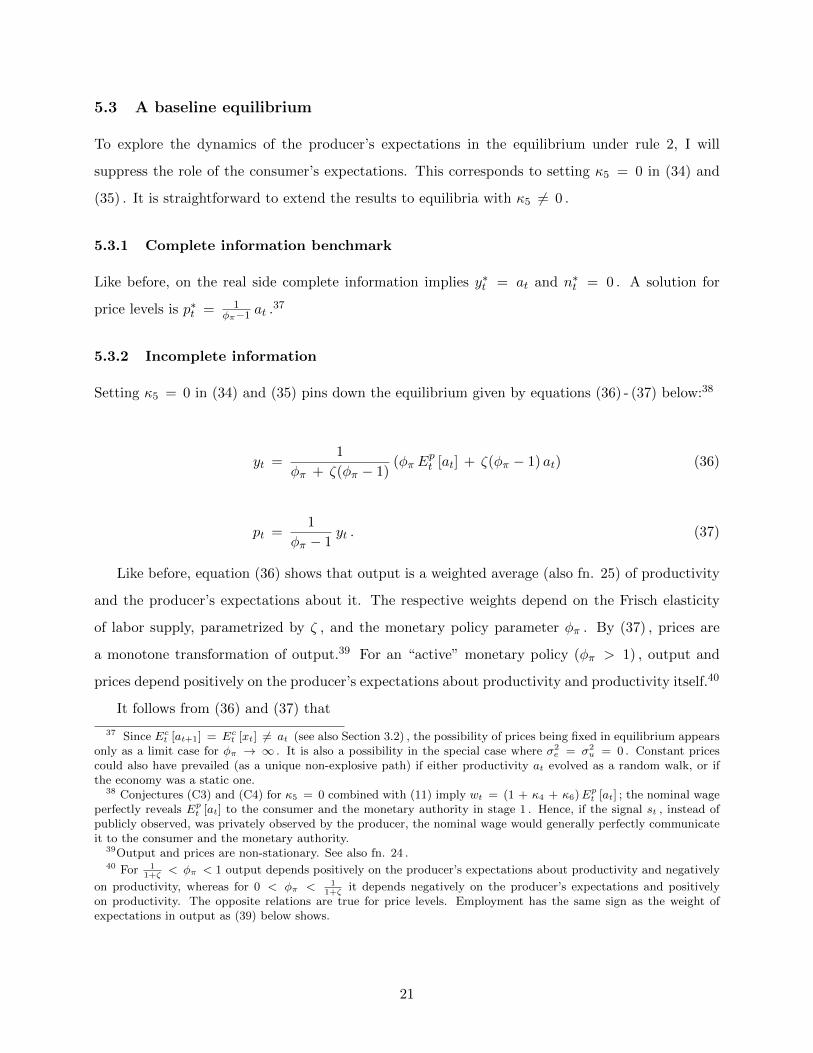
5.3 A baseline equilibrium

To explore the dynamics of the producer’s expectations in the equilibrium under rule 2, I will

suppress the role of the consumer’s expectations. This corresponds to setting κ5 = 0 in (34) and

(35) . It is straightforward to extend the results to equilibria with κ5 6= 0 .

5.3.1 Complete information benchmark

Like before, on the real side complete information implies y∗t = at and n∗t = 0 . A solution for

price levels is p∗t = 1φπ−1 at .37

5.3.2 Incomplete information

Setting κ5 = 0 in (34) and (35) pins down the equilibrium given by equations (36) - (37) below:38

yt =1

φπ + ζ(φπ − 1)(φπ E

pt [at] + ζ(φπ − 1) at) (36)

pt =1

φπ − 1yt . (37)

Like before, equation (36) shows that output is a weighted average (also fn. 25) of productivity

and the producer’s expectations about it. The respective weights depend on the Frisch elasticity

of labor supply, parametrized by ζ , and the monetary policy parameter φπ . By (37) , prices are

a monotone transformation of output.39 For an “active” monetary policy (φπ > 1) , output and

prices depend positively on the producer’s expectations about productivity and productivity itself.40

It follows from (36) and (37) that

37 Since Ect [at+1] = Ect [xt] 6= at (see also Section 3.2) , the possibility of prices being fixed in equilibrium appearsonly as a limit case for φπ → ∞ . It is also a possibility in the special case where σ2

e = σ2u = 0 . Constant prices

could also have prevailed (as a unique non-explosive path) if either productivity at evolved as a random walk, or ifthe economy was a static one.

38 Conjectures (C3) and (C4) for κ5 = 0 combined with (11) imply wt = (1 + κ4 + κ6)Ept [at] ; the nominal wageperfectly reveals Ept [at] to the consumer and the monetary authority in stage 1 . Hence, if the signal st , instead ofpublicly observed, was privately observed by the producer, the nominal wage would generally perfectly communicateit to the consumer and the monetary authority.

39Output and prices are non-stationary. See also fn. 24 .40 For 1

1+ζ< φπ < 1 output depends positively on the producer’s expectations about productivity and negatively

on productivity, whereas for 0 < φπ < 11+ζ

it depends negatively on the producer’s expectations and positivelyon productivity. The opposite relations are true for price levels. Employment has the same sign as the weight ofexpectations in output as (39) below shows.

21

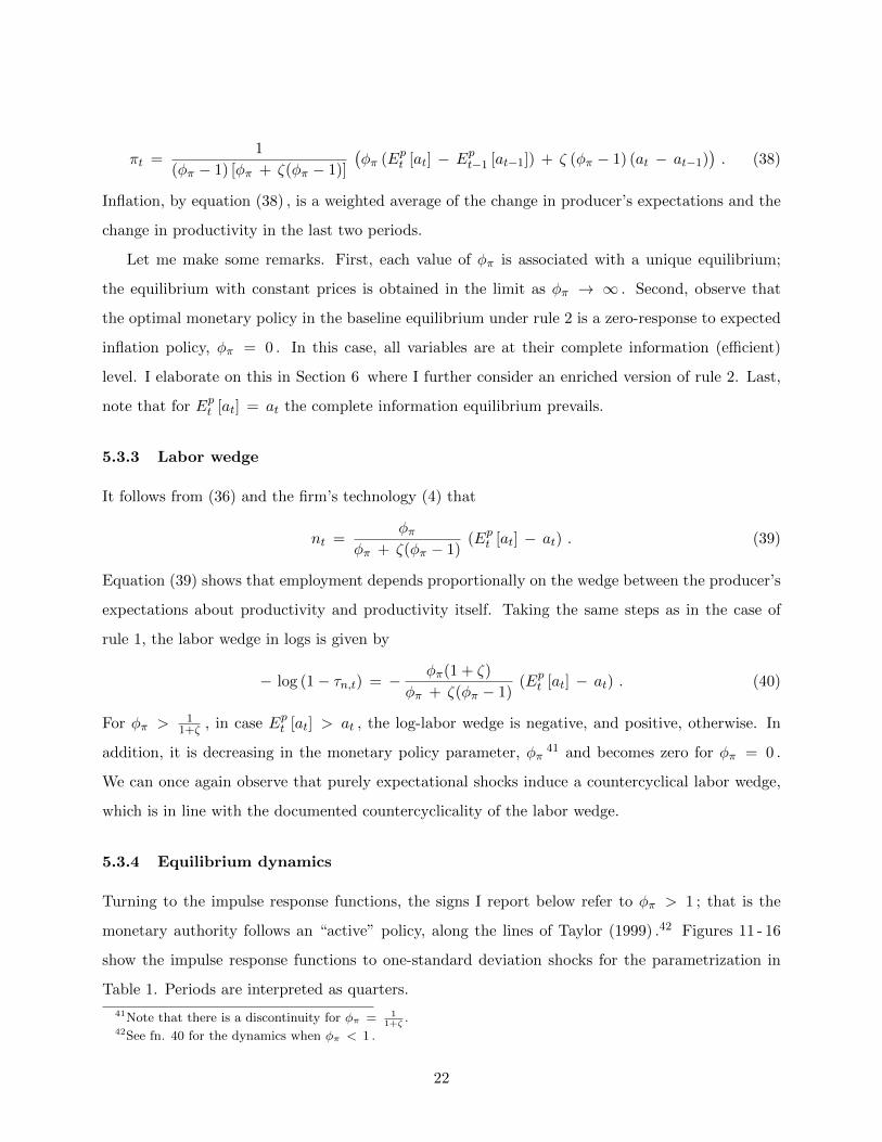
πt =1

(φπ − 1) [φπ + ζ(φπ − 1)]

(φπ (Ept [at] − Ept−1 [at−1]) + ζ (φπ − 1) (at − at−1)

). (38)

Inflation, by equation (38) , is a weighted average of the change in producer’s expectations and the

change in productivity in the last two periods.

Let me make some remarks. First, each value of φπ is associated with a unique equilibrium;

the equilibrium with constant prices is obtained in the limit as φπ → ∞ . Second, observe that

the optimal monetary policy in the baseline equilibrium under rule 2 is a zero-response to expected

inflation policy, φπ = 0 . In this case, all variables are at their complete information (efficient)

level. I elaborate on this in Section 6 where I further consider an enriched version of rule 2. Last,

note that for Ept [at] = at the complete information equilibrium prevails.

5.3.3 Labor wedge

It follows from (36) and the firm’s technology (4) that

nt =φπ

φπ + ζ(φπ − 1)(Ept [at] − at) . (39)

Equation (39) shows that employment depends proportionally on the wedge between the producer’s

expectations about productivity and productivity itself. Taking the same steps as in the case of

rule 1, the labor wedge in logs is given by

− log (1− τn,t) = − φπ(1 + ζ)

φπ + ζ(φπ − 1)(Ept [at] − at) . (40)

For φπ > 11+ζ , in case Ept [at] > at , the log-labor wedge is negative, and positive, otherwise. In

addition, it is decreasing in the monetary policy parameter, φπ41 and becomes zero for φπ = 0 .

We can once again observe that purely expectational shocks induce a countercyclical labor wedge,

which is in line with the documented countercyclicality of the labor wedge.

5.3.4 Equilibrium dynamics

Turning to the impulse response functions, the signs I report below refer to φπ > 1 ; that is the

monetary authority follows an “active” policy, along the lines of Taylor (1999) .42 Figures 11 - 16

show the impulse response functions to one-standard deviation shocks for the parametrization in

Table 1. Periods are interpreted as quarters.

41Note that there is a discontinuity for φπ = 11+ζ

.42See fn. 40 for the dynamics when φπ < 1 .

22

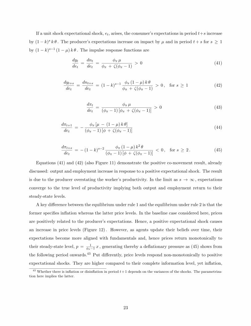
If a unit shock expectational shock, et, arises, the consumer’s expectations in period t+s increase

by (1− k)s k θ . The producer’s expectations increase on impact by µ and in period t+ s for s ≥ 1

by (1− k)s−1 (1− µ) k θ . The impulse response functions are

dytdet

=dntdet

=φπ µ

φπ + ζ(φπ − 1)> 0 (41)

dyt+sdet

=dnt+sdet

= (1− k)s−1φπ (1− µ) k θ

φπ + ζ(φπ − 1)> 0 , for s ≥ 1 (42)

dπtdet

=φπ µ

(φπ − 1) [φπ + ζ(φπ − 1)]> 0 (43)

dπt+1

det= − φπ [µ − (1− µ) k θ]

(φπ − 1) [φ + ζ(φπ − 1)](44)

dπt+sdet

= − (1− k)s−2φπ (1− µ) k2 θ

(φπ − 1) [φ + ζ(φπ − 1)]< 0 , for s ≥ 2 . (45)

Equations (41) and (42) (also Figure 11) demonstrate the positive co-movement result, already

discussed: output and employment increase in response to a positive expectational shock. The result

is due to the producer overstating the worker’s productivity. In the limit as s → ∞ , expectations

converge to the true level of productivity implying both output and employment return to their

steady-state levels.

A key difference between the equilibrium under rule 1 and the equilibrium under rule 2 is that the

former specifies inflation whereas the latter price levels. In the baseline case considered here, prices

are positively related to the producer’s expectations. Hence, a positive expectational shock causes

an increase in price levels (Figure 12) . However, as agents update their beliefs over time, their

expectations become more aligned with fundamentals and, hence prices return monotonically to

their steady-state level, p = 1φπ−1 x , generating thereby a deflationary pressure as (45) shows from

the following period onwards.43 Put differently, price levels respond non-monotonically to positive

expectational shocks. They are higher compared to their complete information level, yet inflation,

43 Whether there is inflation or disinflation in period t+1 depends on the variances of the shocks. The parametriza-tion here implies the latter.

23

by definition, measures changes in price levels between periods.44All effects vanish as s → ∞ .

To pin down the impulse responses of the nominal and the real interest rate (Figure 12) I need

to specify the impulse response of expected inflation:

dEct [πt+1]

det=

ζ(φπ − 1) k θ − φπ (µ− k θ)(φπ − 1) [φπ + ζ(φπ − 1)]

(46)

dEct+s [πt+s+1]

det= (1− k)s−1

φπ (µ− k) + [ζ(φπ − 1) (1− k)] k θ

(φπ − 1) [φπ + ζ(φπ − 1)], for s ≥ 1 . (47)

The nominal interest rate is it+s = φπ Ect+s [πt+s+1] and the real interest rate is rt+s = (φπ −

1)Ect+s [πt+s+1] .45

Inflation expectations increase,46 given the parametrization, resulting in higher nominal and real

interest rates. In the limit s → ∞ , inflation expectations, the nominal, and the real interest rate

all return to their steady-state values.

If a shock to the permanent productivity component εt = 1 arises, the consumer’s expectations

about productivity in period t+s increase by 1 − (1−k)s+1 as (16) implies, whereas the producer’s

expectations increase by 1 − (1− µ) [1− (1− k)s] as (15) implies. The impulse response functions

are

dyt+sdεt

= 1 − (1− k)sφπ (1 − µ)

φπ + ζ(φπ − 1)∈ (0, 1) (48)

dnt+sdεt

= − (1− k)sφπ (1 − µ)

φπ + ζ(φπ − 1)< 0 (49)

dπtdεt

=1

φπ − 1

(1 − φπ (1 − µ)

φπ + ζ(φπ − 1)

)> 0 (50)

dπt+sdεt

= (1− k)s−1φπ (1 − µ) k

(φπ − 1) [φπ + ζ(φπ − 1)]> 0 , for s ≥ 1 . (51)

44A similar result is obtained in Lorenzoni (2005), though not associated with disinflation. The increase in pricescan become less severe and prices can even fall for reasonable values of φπ under an extended forward-looking ruletargeting expected growth in addition to expected inflation. The logic is similar to the rule 1 case: for a given realinterest rate, the greater the weight placed on expected growth, the lower expected inflation will be, controlling forgeneral equilibrium effects.

45 In addition, notice that Ect [yt+s] = Ect [xt] and Ect [πt+s] = 0 for s ≥ 1 . These results follow from (36) and(38) combined with (16) .

46This is unlike the case of rule 1. The difference between the two lies in that rule 1 specifies inflation rather thanprice levels.

24

A unit increase in the permanent productivity shock causes an equivalent change in steady-state

output and no change in steady-state employment. We can see from (48) and (49) (see also Figure

13) that a positive permanent productivity shock causes output to increase by less than one and

employment to fall temporarily. By (40), the labor wedge increases temporarily. This happens

because expectations underreact after a positive permanent productivity shock. As a result, labor

demand shifts inwards and the real wage falls relative to its efficient level. Equation (51) suggests

productivity shocks are inflationary (see also Figure 14). The positive dependence of prices on

expectations for φπ > 1, as (36) and (37) imply, underlies this result. Hence, as expectations

converge to the new permanent productivity level, prices get closer to their steady-state level,

implying inflation along the way.

The impulse response of the consumer’s inflation expectations (also Figure 14) is

dEct+s [πt+s+1]

dεt= (1− k)s

φπ (k − µ) − ζ(φπ − 1) (1− k)

(φπ − 1) [φπ + ζ(φπ − 1)]. (52)

Figure 14 shows that following a permanent productivity shock inflation expectations fall and

so are the nominal and the real interest rate. In the limit as s → ∞ , expectations converge to the

new productivity level, output converges to its new steady state, whereas the remaining variables

return to their pre-shock levels.

A temporary productivity shock causes on impact responses similar to those in the permanent

productivity shock case; from the following period onwards, it only affects the agents’ expectations,

hence the responses resemble the ones in the expectational shock case. The consumer’s expectations

in period t + s increase by (1 − k)s k (1 − θ) , whereas the producer’s expectations are unchanged

on impact, as changes in the temporary productivity component affect their expectations with one-

period lag, and increase by (1− k)s−1 (1− µ) k (1− θ) in period t+ s for s ≥ 1 . In particular, in

period t the responses are

dytdut

=ζ(φπ − 1)

φπ + ζ(φπ − 1)∈ (0, 1) (53)

dntdut

= − φπφπ + ζ(φπ − 1)

< 0 (54)

dπtdut

=ζ

φπ + ζ(φπ − 1)> 0 . (55)

25

In the subsequent periods the responses are

dyt+sdut

=dnt+sdu+t

= (1− k)s−1φπ (1− µ) k (1− θ)φπ + ζ(φπ − 1)

> 0 , for s ≥ 1 (56)

dπt+1

dut= − ζ (φπ − 1) − φπ (1− µ) k(1− θ)

(φπ − 1) [φπ + ζ(φπ − 1)](57)

dπt+sdut

= − (1− k)s−2φπ (1− µ) k2 (1− θ)

(φπ − 1) [φπ + ζ(φπ − 1)]< 0 , for s ≥ 2 . (58)

The response of inflation expectations is given by

dEct [πt+1]

dut=

φπ k (1− θ) − ζ (φπ − 1) [1 − k (1− θ)](φπ − 1)[φπ + ζ(φπ − 1)]

(59)

dEct+s [πt+s+1]

dut= (1− k)s−1

[φπ (µ− k) + ζ(φ− 1) (1− k)] k (1− θ)(φπ − 1) [φπ + ζ(φπ − 1)]

, for s ≥ 1 . (60)

Figures 15 and 16 display the impulse response functions.

5.4 Short-run volatility

In what is a separate exercise, I compare the short-run (one-period) output volatility caused by

purely expectational shocks, et , among the equilibria for the considered interest-rate rules.47 The

parametrization is the one in Table 1 . I normalize to one the short-run output volatility generated

by rule 1 for φy = 0 to make comparisons easier. Table 2 reports the results.

We can see that the baseline case of rule 2 generates considerably higher short-run output

volatility than the considered cases of rule 1 . This can be further increased by assigning a role to

the consumer’s expectations (see also (34)) . Considering the analyzed equilibria for rule 1 , “supply”

shocks (φy = 0.5) generate considerably higher volatility than “demand” shocks (φy = 0) . Indeed,

for φπ high enough so that φπ (1 + ζ) − (1 + φy) > 0 , the short-run output volatility due to

expectational shocks increases in φy .

47Short-run output volatility in the cases of rule 1 and 2, respectively, is

φπ − 1 + k (1− θ)φπ (1 + ζ) − (1 + φy)

µσ2e

φπφπ + ζ (φπ − 1)

µσ2e .

26

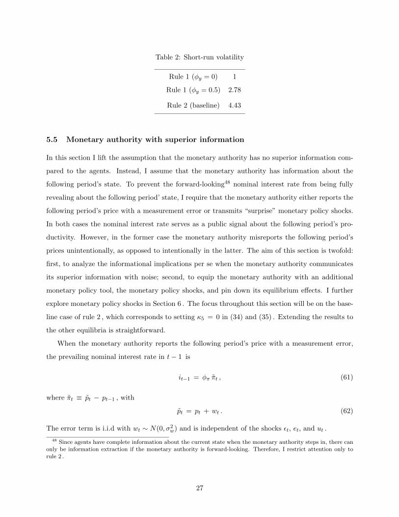
Table 2: Short-run volatility

Rule 1 (φy = 0) 1

Rule 1 (φy = 0.5) 2.78

Rule 2 (baseline) 4.43

5.5 Monetary authority with superior information

In this section I lift the assumption that the monetary authority has no superior information com-

pared to the agents. Instead, I assume that the monetary authority has information about the

following period’s state. To prevent the forward-looking48 nominal interest rate from being fully

revealing about the following period’ state, I require that the monetary authority either reports the

following period’s price with a measurement error or transmits “surprise” monetary policy shocks.

In both cases the nominal interest rate serves as a public signal about the following period’s pro-

ductivity. However, in the former case the monetary authority misreports the following period’s

prices unintentionally, as opposed to intentionally in the latter. The aim of this section is twofold:

first, to analyze the informational implications per se when the monetary authority communicates

its superior information with noise; second, to equip the monetary authority with an additional

monetary policy tool, the monetary policy shocks, and pin down its equilibrium effects. I further

explore monetary policy shocks in Section 6 . The focus throughout this section will be on the base-

line case of rule 2 , which corresponds to setting κ5 = 0 in (34) and (35) . Extending the results to

the other equilibria is straightforward.

When the monetary authority reports the following period’s price with a measurement error,

the prevailing nominal interest rate in t− 1 is

it−1 = φπ πt , (61)

where πt ≡ pt − pt−1 , with

pt = pt + wt . (62)

The error term is i.i.d with wt ∼ N(0, σ2w) and is independent of the shocks εt, et, and ut .

48 Since agents have complete information about the current state when the monetary authority steps in, there canonly be information extraction if the monetary authority is forward-looking. Therefore, I restrict attention only torule 2 .

27

In terms of observables as of stage 2 in period t− 1, this can be expressed as

pt =1

φπ(it−1 + φπ pt−1) .

In the case of monetary policy shocks the nominal interest rate is

it−1 = φπ πt + ωt , (63)

where ω is i.i.d. with ωt ∼ N(0, σ2ω) and is independent of the shocks εt, et, ut, and wt .

Agents now extract

pt = φπ pt + ωt , (64)

which in terms of observables in stage 2 of period t− 1 can be expressed as

pt = it−1 + φπ pt−1 .

5.6 Linear equilibria

Equilibrium is given by equations (36) - (38) . The state of the economy is now augmented by the

public signal about period t’s productivity which the monetary authority transmits. I denote this

by zt in the case of a measurement error and zt in the case of a monetary policy shock. The state

can sufficiently be described then by Ωt =(aτtτ=0 , sτtτ=0 , zt

), replacing Ωt with Ωt and zt

with zt in the case of a monetary policy shock. What distinguishes the two cases is the information

set of the monetary authority; in the case of measurement errors it is Imt = Ωt \ zt , whereas

in the case of monetary policy shocks it is Imt = Ωt . That is, in the latter case, the monetary

authority takes into account the effects of the signal it transmits. I assume it is common knowledge

what the case is each time a shock hits. As I show in Appendix A.4.1, the endogenous public signals

associated with the two cases are

zt = at +φπ + ζ(φπ − 1)

ζwt (65)

zt = at +φπ + ζ(φπ − 1)

φπ ζωt . (66)

Agents (perfectly) disentangle the endogenous public signals upon the realization of the public

signal st in stage 1 of period t .49 The producer’s information set then becomes Ipt,1 = Ωt \ at ,

49 This happens because they know the stochastic process of prices given by (37) .

28

whereas the consumer’s Ict = Ωt . As I show in Appendix A.4.1, the producer’s expectations about

productivity are

Ept [at | Ipt,1] = δ Ept

[xt | Ipt,1 \ zt

]+ (1− δ) zt , (67)

where δ is a coefficient in (0, 1) (respectively use δ, zt and Ωt in the case of a monetary policy

shock) . Importantly, δ and δ depend on the monetary policy parameter φπ .50

It is apparent from (65) and (66) that the economy’s response to measurement errors and

monetary policy shocks is very similar. In particular, for φπ > 1 positive interest rate shocks raise

the producer’s expectations about productivity in the following period. This happens because for

φπ > 1 prices are positively related to productivity. Therefore, a higher nominal interest rate

overstates the following period’s price and leads the producer to partially attribute it to an increase

in productivity.51

5.7 Equilibrium dynamics

The dynamics when shocks εt, et, and ut are realized are very similar to the ones in Section 5.3.4 .

Unlike there, the effects of a measurement error or a monetary policy shock last only one period.

This is because it generates a signal about at, which consumers learn and producers realize once

the labor decision is made . If a shock wt = 1 arises, the impact responses are

dytdwt

=dntdwt

=φπ (1− δ)

ζ> 0 (68)

dptdwt

=dπtdwt

= −dπt+1

dwt=

φπ (1− δ)ζ (φπ − 1)

> 0 . (69)

It can be seen from (68) and (69) that interest rate shocks boost output and prices. These

responses are in the same direction as the ones after a shock to the public signal st . This is because

measurement errors and monetary policy shocks serve as purely expectational shocks: when positive,

50 The case analyzed in Section 3 corresponds to δ = 1 which would prevail if the conditional variance of theendogenous signals was infinite.

51 In case the monetary authority has no superior information and this is common knowledge, monetary policyshocks have no real effects because they are unanticipated by both agents, hence they have no effect on the labordecision in stage 1 . They can immediately be extracted by the agents which implies they have no effect on theconsumer’s inflation and output expectations for the following period. As a result, they only affect the current price,in a co-monotone way for φπ > 1 . On the contrary, in the superior information case agents extract monetary policyshocks with one-period lag, hence their nominal effects are realized in the following period. In addition, monetarypolicy shocks have real effects since they are not simultaneously fully extracted by both agents.

29

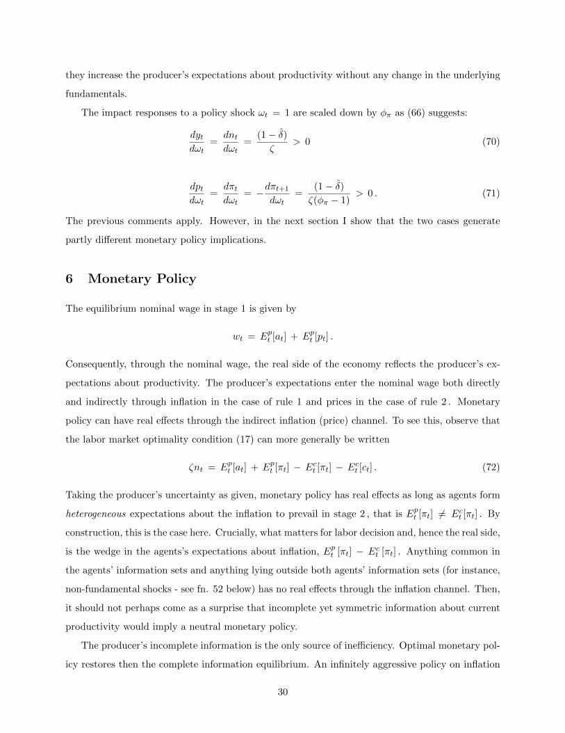
they increase the producer’s expectations about productivity without any change in the underlying

fundamentals.

The impact responses to a policy shock ωt = 1 are scaled down by φπ as (66) suggests:

dytdωt

=dntdωt

=(1− δ)ζ

> 0 (70)

dptdωt

=dπtdωt

= −dπt+1

dωt=

(1− δ)ζ(φπ − 1)

> 0 . (71)

The previous comments apply. However, in the next section I show that the two cases generate

partly different monetary policy implications.

6 Monetary Policy

The equilibrium nominal wage in stage 1 is given by

wt = Ept [at] + Ept [pt] .

Consequently, through the nominal wage, the real side of the economy reflects the producer’s ex-

pectations about productivity. The producer’s expectations enter the nominal wage both directly

and indirectly through inflation in the case of rule 1 and prices in the case of rule 2 . Monetary

policy can have real effects through the indirect inflation (price) channel. To see this, observe that

the labor market optimality condition (17) can more generally be written

ζnt = Ept [at] + Ept [πt] − Ect [πt] − Ect [ct] . (72)

Taking the producer’s uncertainty as given, monetary policy has real effects as long as agents form

heterogeneous expectations about the inflation to prevail in stage 2 , that is Ept [πt] 6= Ect [πt] . By

construction, this is the case here. Crucially, what matters for labor decision and, hence the real side,

is the wedge in the agents’s expectations about inflation, Ept [πt] − Ect [πt] . Anything common in

the agents’ information sets and anything lying outside both agents’ information sets (for instance,

non-fundamental shocks - see fn. 52 below) has no real effects through the inflation channel. Then,

it should not perhaps come as a surprise that incomplete yet symmetric information about current

productivity would imply a neutral monetary policy.

The producer’s incomplete information is the only source of inefficiency. Optimal monetary pol-

icy restores then the complete information equilibrium. An infinitely aggressive policy on inflation

30

policy implies πt = 0 and only removes the indirect, inflation (price) channel of expectations. As

a result, it is typically suboptimal.

By direct implication of (14) , the complete information equilibrium is restored if and only if

Ept [at] + Ept [πt] − (πt + at) = 0 (73)

Ept [at] + Ept [pt] − (pt + at) = 0 , (74)

for rules 1 and 2 , respectively.

It follows that monetary policy succeeds, not by removing the producer’s uncertainty, but rather

by making it irrelevant. To see this, note that inflation (prices) depends on productivity and agents’

expectations in a way decided by monetary policy. Optimal monetary policy manipulates inflation

in such a way that the producer correctly anticipates his stage-2 revenue, which is all he is interested

in.

One would argue that the inefficiency here arises exactly because of agents’s asymmetric infor-

mation; if agents had incomplete yet symmetric information, then the complete information equilib-

rium would prevail. However, this is true only because of logarithmic preferences in consumption; in

more general environments, the producer’s incomplete information would suffice. Nevertheless, it is

asymmetric, rather than incomplete but symmetric, information in combination with the existence

of a nominal bond market that enables the monetary authority to drive the economy closer to the

complete information equilibrium. If a real bond market was in the place of the nominal bond

market, then the inflation (price) channel would be absent, and there would be no way to drive the

economy to the first best.

Optimal policy here has different implications from the one in Weiss (1980) which implies that

prices perfectly communicate fundamentals. By construction, this is a nonexistent possibility here.

However, this paper shares with Weiss (1980), King (1982) and Lorenzoni (2010) the insight that,

at the time the labor decision is made, it is asymmetric, as opposed to incomplete but symmetric,

information about variables the monetary policy will be based on that breaks the policy irrelevance

proposed in Sargent and Wallace (1975, 1976) . Implicit in this is that the monetary authority is

more informed when it steps in than the least informed agent (here, the producer) at the time

the labor decision is made. This is true here since the time advantage of the monetary authority

is essentially an informational advantage; in fact, the monetary authority perfectly observes or

extracts the variables in question (inflation, output, current productivity) when it steps in.

31

Crucially, that inflation stabilization is suboptimal is in contrast with the baseline case in Loren-

zoni (2009) in which the limit φπ → ∞ restores the efficient equilibrium. In Lorenzoni (2009) ,

producers have complete information, however nominal rigidities prevent prices from fully absorbing

the consumer’s expectations about long-run productivity. Stabilizing inflation resolves this. In con-

trast, here prices flexibly adjust, however producers have incomplete information about productiv-

ity and, consequently, their (stage-2) revenue; stabilizing inflation only eliminates their uncertainty

about inflation but not about their revenue.

Below I consider both interest-rate rules and explore how the monetary authority can mitigate

the effects of incomplete information and drive the economy closer to its complete information

counterpart in each case. In the context of rule 2 , I design policy targets which restore the complete

information equilibrium for any choice of policy parameters.52

6.1 Rule 1

If interest-rate rule 1 is followed, setting φπ = 1 − k (1 − θ) is optimal; however, this policy is

unrealistic as it requires the monetary authority to be fully aware of the agents’ learning problems

which is hardly realistic. Crucially, in the limit as φπ → ∞, πt → 0 ;53 inflation is constant and

the indirect (inflation/price) channel of expectations, through which the consumer’s expectations

also operate, is muted. However, even in this limit case, the producer’s expectations continue to

matter via the direct channel. Hence, inflation stabilization can at best eliminate the uncertainty

arising through the inflation channel and, as such, is suboptimal.

An implication of Section 5.4 is that, for moderate values of φy , short-run output volatility

due to purely expectational shocks increases in φy . However, perhaps not surprisingly, in the limit

φy → ∞ , the economy is at its complete information counterpart; a policy infinitely responsive to

deviations of output from its complete information level is therefore optimal.

52My focus so far has been on the effects of purely expectational shocks as well on those of productivity shocks.However, a fair question, especially when it comes to monetary policy, is about the possible presence of indeterminacies.The answer is that here there is no real indeterminacy. To see this, first note that the labor decision is intratemporaland is anyway made before inflation prevails. Turning to inflation, even if it is indeterminate, i.e. susceptible topossibly non-fundamental (“sunspot”) shocks, since the “sunspot” shocks lie outside the information sets of bothagents, they cannot affect the labor decision in stage 1 , i.e. they cannot have real effects (see (72) and the analysisthat comes with it) . Nevertheless, there may well be nominal indeterminacy. To rule out “sunspot” shocks in thecase, for instance, of rule 1, on which the positive part of this paper is based , we would need φπ > 1 . But I shouldrepeat here, that I abstract from such considerations.

53 As φπ increases, the sign of the change in the weight of the producer’s expectations, ξ1 , is given by the sign of− (1 +φy) + [1 − k (1− θ)] (1 + ζ) (see also (19) and (21)) . It is negative for a high enough φy relative to the inverse

Frisch elasticity ζ , while there is a discontinuity at1+φy1+ζ

.

32

6.2 Rule 2

A first policy implication generated by the equilibrium analysis (see Section 5) is that a forward-

looking rule, like rule 2 , invites multiple equilibria in which the consumer’s expectations is arbitrarily

specified, which is not the case when a contemporaneously-looking rule is followed.54 Second, as I

showed in Section 5.4 , the short-run volatility of output due to expectational shocks is substantially

higher for forward-looking rules than for contemporaneously-looking ones, for the parametrization

in Table 1 .

I initially consider the baseline equilibrium in which the consumer’s expectations have no role.55

This corresponds to setting κ5 = 0 in (34) . Observe in (36) that the weight of output placed on

producer’s expectations is κ4 = φπφπ + ζ (φπ−1) , whereas the weight placed on productivity is 1 − κ4 .

The former decreases in φπ (see also fn. 41) ; the greater φπ , the weaker the indirect (price) channel

of expectations will be. In the limit as φπ → ∞ , prices are constant. As in the previous case, only

the indirect channel of expectations is muted, therefore inflation stabilization is suboptimal.

The focus so far has been on active policies, which correspond to the monetary authority setting

φπ > 1 . However, setting φπ = 0 in (36) and (37) returns yt = at and pt = − at ; a Friedman-

rule policy completely eliminates the role of expectations and keeps the economy at its complete

information level. To provide an intuition for this, observe that for φπ < 11+ζ the price effect

becomes negative, which implies the indirect channel effect mitigates the direct one. For φπ = 0,

the two effects precisely offset each other, rendering, therefore, incomplete information irrelevant in

equilibrium. Notably, such a policy implies that the producer’s revenue is constant across states:

high prices prevail for low productivities and vice versa. Summarizing the above, the Friedman rule,

for different from the usual reasons, emerges as an optimal policy; however, if an active policy is to

be pursued, then it should be as aggressive on inflation as possible.

Next, I analyze monetary policy when the monetary authority has superior information. As we

saw earlier, the monetary authority can either, unintentionally, report prices with a measurement

error or, intentionally, fuel the economy with “surprise” monetary policy shocks. A straightforward

option for a “benevolent” monetary authority in the latter case is to use monetary policy shocks to

eliminate the producer’s expectational errors. However, I will focus on the monetary policy param-

eters that can insulate the economy against measurement errors and can serve as a commitment

device against monetary policy shocks.

54At least, I have failed to find other linear equilibria for rule 1 .55See fn. 58 below for the general case.

33

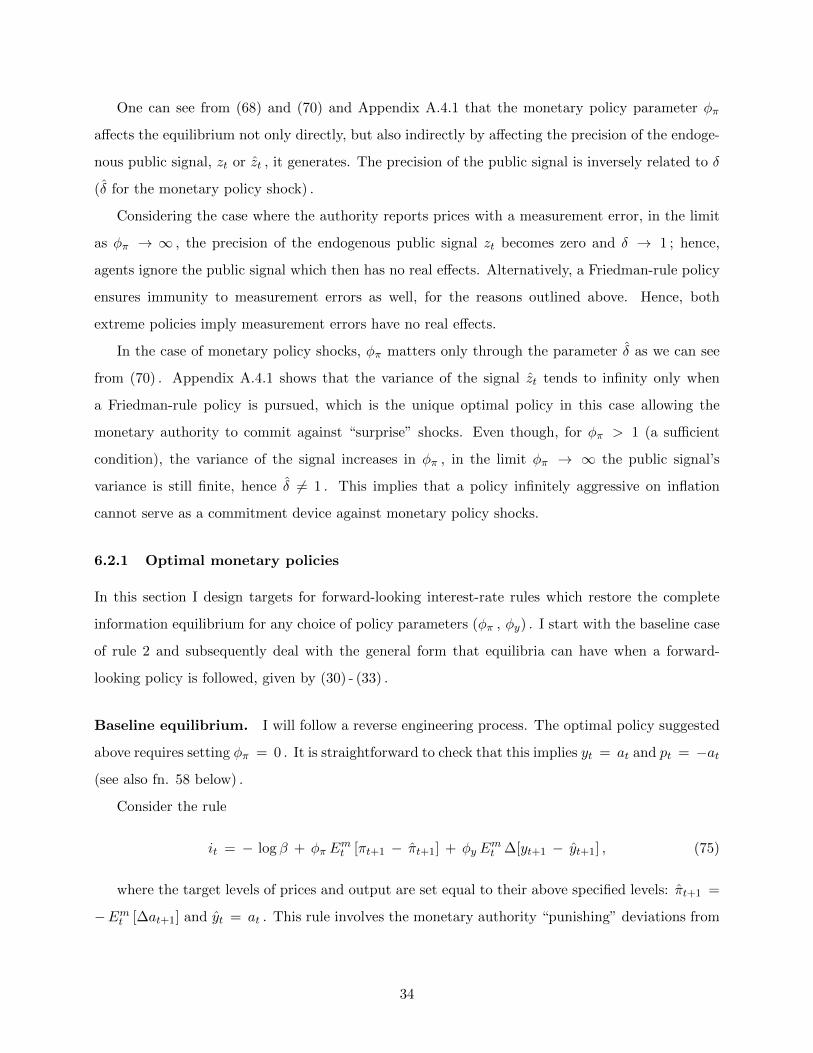
One can see from (68) and (70) and Appendix A.4.1 that the monetary policy parameter φπ

affects the equilibrium not only directly, but also indirectly by affecting the precision of the endoge-

nous public signal, zt or zt , it generates. The precision of the public signal is inversely related to δ

(δ for the monetary policy shock) .

Considering the case where the authority reports prices with a measurement error, in the limit

as φπ → ∞ , the precision of the endogenous public signal zt becomes zero and δ → 1 ; hence,

agents ignore the public signal which then has no real effects. Alternatively, a Friedman-rule policy

ensures immunity to measurement errors as well, for the reasons outlined above. Hence, both

extreme policies imply measurement errors have no real effects.

In the case of monetary policy shocks, φπ matters only through the parameter δ as we can see

from (70) . Appendix A.4.1 shows that the variance of the signal zt tends to infinity only when

a Friedman-rule policy is pursued, which is the unique optimal policy in this case allowing the

monetary authority to commit against “surprise” shocks. Even though, for φπ > 1 (a sufficient

condition), the variance of the signal increases in φπ , in the limit φπ → ∞ the public signal’s

variance is still finite, hence δ 6= 1 . This implies that a policy infinitely aggressive on inflation

cannot serve as a commitment device against monetary policy shocks.

6.2.1 Optimal monetary policies

In this section I design targets for forward-looking interest-rate rules which restore the complete

information equilibrium for any choice of policy parameters (φπ , φy) . I start with the baseline case

of rule 2 and subsequently deal with the general form that equilibria can have when a forward-

looking policy is followed, given by (30) - (33) .

Baseline equilibrium. I will follow a reverse engineering process. The optimal policy suggested

above requires setting φπ = 0 . It is straightforward to check that this implies yt = at and pt = −at

(see also fn. 58 below) .

Consider the rule

it = − log β + φπ Emt [πt+1 − πt+1] + φy E

mt ∆[yt+1 − yt+1] , (75)

where the target levels of prices and output are set equal to their above specified levels: πt+1 =

−Emt [∆at+1] and yt = at . This rule involves the monetary authority “punishing” deviations from

34

the efficient inflation and growth rates.56,57

Taking the same steps as in the derivations of (36) - (37) shows that any chosen coefficients

(φπ , φy) can drive the economy to its efficient level. The Friedman rule is a special case obtained

for φπ = φy = 0 .

Multiple equilibria. Consider the interest-rate rule given by (75) . Make the following modifi-

cation:

πt+1 = κ7Emt [∆at+1] (76)

κ7 = − 1 +φπ − 1

φπk (1− θ)κ5 . (77)

This rule drives the economy to its complete information counterpart. Once again, observe that

the inflation and growth targets are related to their complete information levels.58 The proposed

rule is invariant to changes in φy , whereas, as (77) shows, it adjusts to the chosen value of φπ .59

To get an intuition for the latter, first use the former result and set φy = 0 in order to bring the

equilibrium closer to the equilibrium given by (34) - (35) . Then observe in (34) that the real effects

of the consumer’s expectations depend on the monetary authority’s response to expected inflation,

φπ . Hence, the targets in the suggested policy (75) - (77) also need to adjust accordingly to changes

in φπ . All derivations are collected in Appendix A.5 .

The monetary authority can extract the role of the consumer’s expectations, parametrized by κ5 ,

and productivity at by observing output and prices (see also (35)) when it steps in; subsequently, it

56 As already emphasized, the authority has complete information when it sets the nominal interest rate.57Orphanides (2003) discusses the benefits of targeting output growth.58 To get an intuition for this, recall that the efficient equilibrium requires ξ3 = 0 ; this implies κ4 = 0 by (32)

and κ6 = 1φπ−1

by (33) . Given these, we can see in (34) that ξ3 = 0 prevails for φπ such that κ5 = − 1k (1−θ)

φπφπ−1

.Then, the equilibrium is

yt = at (78)

pt =1

φπ − 1at −

1

k (1− θ)φπ

φπ − 1Ect [xt] . (79)

The rule given by (75) - (77) and yt = at yields

yt = at (80)

pt = − [1 + k (1− θ)κ5] at + κ5Ect [xt] . (81)

Setting κ5 = − 1k (1−θ)

φπφπ−1

returns (78) - (79) .59The rule will not adjust to changes in φπ for κ5 = 0 , as already shown.

35

can invoke the rule given by (75) - (77) and yt = at and restore the complete information equilibrium

for any choice of policy parameters (φπ , φy) .

Last, observe that setting κ5 = 0 returns κ6 = −1 and κ7 = −1 , which correspond to the

baseline rule (75) .

7 Conclusion

This paper has reconsidered the nature of purely expectational shocks within a competitive, cash-

less, monetary economy. Asymmetric information about current fundamentals is the driving force

in the model. Informational asymmetries lead agents to form heterogeneous expectations about in-

flation; as a result, monetary policy and consumers’ expectations have real effects through inflation.

Traditionally, expectational shocks are viewed as Keynesian demand shocks: when positive, they

increase output, employment and inflation. I have shown that this interpretation remains a possi-

bility but is not the only one; expectational shocks can cause business cycle patterns associated with

supply shocks: when positive, they increase output and employment and they lower inflation. Such

an interpretation seems in line with the low inflation and the high cyclical employment in the mid-

80s and the second half of the 90s, which are recalled as periods of exuberant optimism. Whether

expectational shocks manifest themselves as demand or supply shocks reflects the monetary policy

pursued.

I have considered different interest-rate rules and shown that forward-looking rules generate

multiple equilibria in which consumers’ expectations have an arbitrary role. Further to this, expec-

tational shocks cause substantially higher short-run output volatility under forward-looking policies

than under “contemporaneous” ones. Inflation stabilization per se is typically suboptimal, as it can

at best eliminate uncertainty arising through prices. Optimal monetary policies manipulate inflation

so that the producer correctly anticipates his revenue. In this way, producers’ incomplete informa-

tion about productivity becomes irrelevant. I have designed targets for forward-looking interest-rate

rules which restore the complete information equilibrium for any chosen policy parameters.

Recovering purely expectational shocks from the data will shed light on their seemingly shifting

nature. Of course, the literature on the identification of expectational shocks remains far from

settled (for example, Beaudry and Portier (2006), Blanchard et al. (2009) and Barsky and Sims

(2011a,b)). On the policy front, introducing capital, investment and credit constraints is a rather

natural extension with potentially promising monetary policy implications.

36

A Omitted derivations

A.1 Equilibrium definition and agents’ problems

Equilibrium definition. A rational expectations equilibrium under an interest-rate rule Q (Ψt)

consists of prices Pt (Ψt) , Wt (Ψt \at) , an allocation Ndt (Ψt \at) , Yt (Ψt) for the producer

and an allocation Ct (Ψt) , Nst (Ψt) , Bt+1 (Ψt) for the consumer such that:

1. Ndt (Ψt \ at) , Yt (Ψt) solves the producer’s problem, laid out below, at prices Pt (Ψt) ,

Wt (Ψt \ at) , Q (Ψt) .

2. Ct (Ψt) , Nst (Ψt) , Bt+1 (Ψt) solves the consumer’s problem, laid out below, at prices Pt (Ψt) ,

Wt (Ψt \ at) , Q (Ψt) .

3. All markets clear: Yt = Ct, Ndt = N s

t , Bt+1 = 0 for all t with B0 = 0 .

Producer’s problem. Stage 2 profits of the consumer-owned firm are given by Πt = Pt Yt −

WtNt , where Yt = AtNt .

In stage 1 of each period t , the producer chooses Nt ≥ 0 to maximize the firm’s expected profits

evaluated according to the consumer’s Lagrange multiplier denoted λt :

Ept [λt Πt] .

Expectations are with respect to the information set of the producer in stage 1 which, as specified

in the main text, is Ipt,1 = Ψt \ at . The maximization problem does not yield a solution for

Wt <Ept [λt Pt At]

Ept [λt].

The producer accommodates any labor supply for

Wt =Ept [λt PtAt]

Ept [λt]. (82)

Since, technology is linear in the worker’s productivity, the scale of production is pinned down by

the labor supply side. Put differently, the producer commits to accommodate any labor supplied

which will pin down the output produced as long as the nominal wage is the one given by (82) .

The case in which the LHS of (82) is greater than the RHS implies Nt = 0 which in turn implies

Yt = 0 , which is not possible in equilibrium as the consumer’s problem requires Ct > 0 .

On another note, since production takes place after the nominal wage is announced and depends

on the consumer/worker’s productivity, Yt in the definition of equilibrium above is a function of the

state Ψt rather than the producer’s information set in stage 1 , Ψt \ at .

37

Consumer’s problem. Given B0 = 0, the consumer solves the following problem:

maxCt , Nt , Bt+1∞t=0

Ec0

∞∑t=0

(logCt −

N1+ζt

1 + ζ

)

subject to the sequence of budget constraints

PtCt + QtBt+1 = Bt + WtNt + Πt ,

and a no-Ponzi-scheme constraint (requiring that Bt+1 > −Γ for any Γ > 0 at all t would do since

in equilibrium Bt+1 = 0 for all t) . The FOCs with respect to Ct, Nt, and Bt+1 respectively are:

1

Ct= λt Pt (83)

N ζt = λtWt (84)

Qt = βEct [λt+1]

λt, (85)

where, as noted above, λt is the current-value Lagrange multiplier associated with the period-t

budget constraint. Expectations are with respect to the information set of the consumer which

coincides with the state Ψt (see also the analysis in the main text) . I have made no distinction

between stages 1 and 2 for the consumer as he has the same information in both stages. Combining

(83) with (84) and (83) with (85) yields, respectively,

N ζt =

Wt

PtCt(86)

Qt = β Ect

[PtPt+1

CtCt+1

]. (87)

In addition, the no-Ponzi-scheme condition and the fact that nominal bonds are in zero net-supply

imply Bt+1 = 0 in equilibrium.

A.2 Kalman filter

Let me start with the consumer’s case which is easier to handle. The consumer’s information set

is Ict = Ict−1 ∪ st, at . Suppose the consumer’s prior in period t is xt | Ict−1 ∼ N(0 , σ2x) , where

38

σ2x ≡ V arct−1 [xt] . Before applying Bayes’ Law, recall that all shocks are serially uncorrelated,

mutually independent, and normally distributed. The consumer’s posterior is

xt | Ict−1 ∼ N

(0 ,

(1

σ2x+

1

σ2e+

1

σ2u

)−1).

This implies the following period’s prior is

xt+1 | Ict ∼ N

(0 ,

(1

σ2x+

1

σ2e+

1

σ2u

)−1+ σ2ε

).

Using σ2x to denote V arct [xt+1] , it follows that

σ2x =

(1

σ2x+

1

σ2e+

1

σ2u

)−1+ σ2ε . (88)

I will assume the consumer’s prior in period 0 is x0 | −1 ∼ N(0 , σ2x) , where I let σ2x denote

the solution (a fixed point) to the Riccati equation (88) . This implies the learning problem of the

agents is at its steady state when time commences. Turning to the coefficients in (16) , let

k ≡1σ2e

+ 1σ2u

1σ2x

+ 1σ2e

+ 1σ2u

,

denote the Kalman gain term, that is the precision of new information relative to the prior’s pre-

cision. This is time-invariant due to the consumer’s learning problem being at its steady state. In

addition, let θ ≡1

σ2e1

σ2e+ 1

σ2u

, denote the relative precision of the signal st within the new information

st, at .

Turning to the producer’s learning problem, recall from the analysis in the main text that agents

have the same information set at the end of each period, that is Ipt−1,2 = Ict−1 . As as result, they

have the same prior in the following period. However, their information sets differ in stage 1 . In

particular, the producer’s information set is Ipt,1 = Ipt−1,2 ∪ st . Letting µ ≡1

σ2e1

σ2x+ 1

σ2e

yields the

coefficient in (15) .

A thorough demonstration of the Kalman filter can be found in Anderson and Moore (1979),

Harvey (1989) and Technical Appendix B in Ljungqvist and Sargent (2004) .

39

A.3 Equilibrium under Rule 1

Let me elaborate first on the filtering problems of the agents. The producer’s and the consumer’s

expectations, respectively, are (see also (15) and (16)) :

Ept [at] = Ept,1 [xt] = (1− µ)Ept−1,2 [xt−1] + µ st

Ept,2 [xt] = Ect [xt] = (1− k)Ect−1 [xt−1] + k [θ st + (1− θ) at] .

Then, the consumer’s expectations in period t of the producer’s expectations in t+ 1 are given by

Ect [Ept+1 [at+1] ] = Ect [xt] , (89)

and the producer’s expectations in period t of the consumer’s expectations in t are given by

Ept [Ect [xt] ] = (1−k)Ect−1 [xt−1] + k [θ st + (1−θ)Ept [at]] = Ect [xt] + k (1−θ) (Ept [at]− at) . (90)

Substituting conjectures (C1), (C2), and (90) in (17) implies

ζnt = (1 + κ3 − ξ1)Ept [at] + κ2 k (1− θ) (Ept [at] − at) − (κ3 + ξ2) at . (91)

Substituting (91) in the firm’s technology, yt = at + nt , using market clearing, yt = ct , and,

subsequently, matching coefficients with conjecture (C1) yields

ξ1 =1 + κ3 + κ2 k (1− θ)

1 + ζ(92)

ξ2 =ζ − κ3 − κ2 k (1− θ)

1 + ζ. (93)

Observe that

ξ1 + ξ2 = 1 , (94)

a direct consequence of preferences logarithmic in consumption.

Turning to the Euler equation (18), conjectures (C1) and (C2) combined with (89) imply

Ect [ct+1] − ct = − ξ1Ept [at] + (ξ1 + ξ2)Ect [xt] − ξ2 at (95)

it − Ect [πt+1] = (φy ξ1 + φπ κ1)Ept [at] + [−κ1 + (φπ − 1)κ2 − κ3]E

ct [xt] + [φy ξ2 + φπ κ3 − φy] at .

(96)

40

Matching coefficients in (95) and (96) yields

− ξ1 =φy ξ1 + φπ κ1 (97)

ξ1 + ξ2 = − κ1 + (φπ − 1)κ2 − κ3 (98)

− ξ2 =φy ξ2 + φπ κ3 − φy . (99)

Summing (97) - (99) across sides and using (94) yields

κ1 + κ2 + κ3 = 0 , (100)

whereas summing across (97) and (99) and again using (94) yields

κ1 + κ3 = − 1

φπ, (101)

which are equations (23) and (24) , respectively, in the main text.

Solving (93), (94) and (97) - (99) for ξ1 , ξ2 , κ1 , κ2 , κ3 returns (19) - (21) in the main text.

A.4 Equilibria under Rule 2

Equations (30) - (31) can be obtained by combining the equilibrium labor decision (14) with the

firm’s technology and market clearing. They coincide with (92) - (94), derived in Appendix A.3

above (one only needs to replace ξ1 with ξ3 , ξ2 with ξ4 , κ2 with κ5 , and κ3 with κ6) .

Turning to the Euler equation, conjectures (C3) - (C4) imply Ect [ct+1] = (ξ3 + ξ4)Ect [xt] and

Ect [pt+1] = (κ4 + κ5 + κ6)Ect [xt]. Then the LHS and the RHS of the Euler equation (13) after

taking into account that Imt = Ict (equation (29) in the main text) become, respectively,

Ect [ct+1] − ct = (ξ3 + ξ4)Ect [xt] − ξ3E

pt [at] − ξ4 at (102)

it − Ect [πt+1] = (φπ − 1)Ect [πt+1] = (φπ − 1) [(κ4 + κ6)Ect [xt] − κ4E

pt [at] − κ6 at] . (103)

Matching coefficients in (102) - (103) and using (31) yields (32) - (33) .

A.4.1 Omitted derivations in Section 5.5

First, I deal with the case in which the monetary authority reports the following period’s prices

with a measurement error. Next, I follow the same process in the case of a monetary policy shock.

Recall that what distinguishes the two cases is the information set of the monetary authority.

41

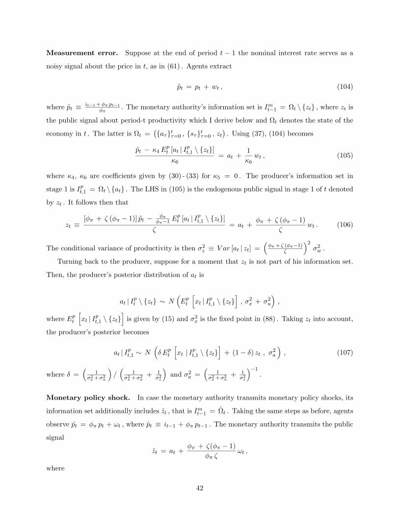
Measurement error. Suppose at the end of period t − 1 the nominal interest rate serves as a

noisy signal about the price in t, as in (61) . Agents extract

pt = pt + wt , (104)

where pt ≡ it−1 +φπ pt−1

φπ. The monetary authority’s information set is Imt−1 = Ωt \ zt , where zt is

the public signal about period-t productivity which I derive below and Ωt denotes the state of the

economy in t . The latter is Ωt =(aτtτ=0 , sτtτ=0 , zt

). Using (37), (104) becomes

pt − κ4Ept [at | Ipt,1 \ zt]κ6

= at +1

κ6wt , (105)

where κ4, κ6 are coefficients given by (30) - (33) for κ5 = 0 . The producer’s information set in

stage 1 is Ipt,1 = Ωt \at . The LHS in (105) is the endogenous public signal in stage 1 of t denoted

by zt . It follows then that

zt ≡[φπ + ζ (φπ − 1)] pt − φπ

φπ−1 Ept [at | Ipt,1 \ zt]

ζ= at +

φπ + ζ (φπ − 1)

ζwt . (106)

The conditional variance of productivity is then σ2z ≡ V ar [at | zt] =(φπ + ζ (φπ−1)

ζ

)2σ2w .

Turning back to the producer, suppose for a moment that zt is not part of his information set.

Then, the producer’s posterior distribution of at is

at | Ipt \ zt ∼ N(Ept

[xt | Ipt,1 \ zt

], σ2x + σ2u

),

where Ept

[xt | Ipt,1 \ zt

]is given by (15) and σ2x is the fixed point in (88) . Taking zt into account,

the producer’s posterior becomes

at | Ipt,1 ∼ N(δ Ept

[xt | Ipt,1 \ zt

]+ (1− δ) zt , σ2a

), (107)

where δ =(

1σ2x+σ2

u

)/(

1σ2x+σ2

u+ 1

σ2z

)and σ2a =

(1

σ2x+σ2

u+ 1

σ2z

)−1.

Monetary policy shock. In case the monetary authority transmits monetary policy shocks, its

information set additionally includes zt , that is Imt−1 = Ωt . Taking the same steps as before, agents

observe pt = φπ pt + ωt , where pt ≡ it−1 + φπ pt−1 . The monetary authority transmits the public

signal

zt = at +φπ + ζ(φπ − 1)

φπ ζωt ,

where

42

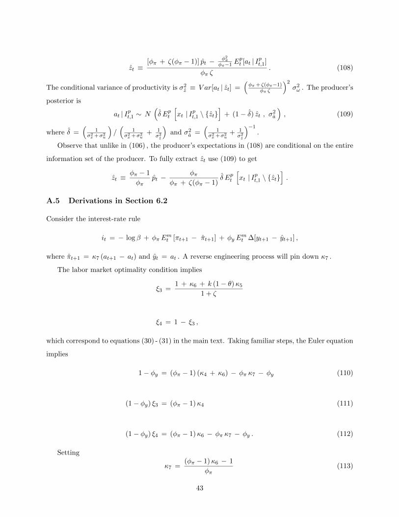
zt ≡[φπ + ζ(φπ − 1)] pt − φ2π

φπ−1 Ept [at | Ipt,1]

φπ ζ. (108)

The conditional variance of productivity is σ2z ≡ V ar[at | zt] =(φπ + ζ(φπ−1)

φπ ζ

)2σ2ω . The producer’s

posterior is

at | Ipt,1 ∼ N(δ Ept

[xt | Ipt,1 \ zt

]+ (1− δ) zt , σ2a

), (109)

where δ =(

1σ2x+σ2

u

)/(

1σ2x+σ2

u+ 1

σ2z

)and σ2a =

(1

σ2x+σ2

u+ 1

σ2z

)−1.

Observe that unlike in (106) , the producer’s expectations in (108) are conditional on the entire

information set of the producer. To fully extract zt use (109) to get

zt ≡φπ − 1

φπpt −

φπφπ + ζ(φπ − 1)

δ Ept

[xt | Ipt,1 \ zt

].

A.5 Derivations in Section 6.2

Consider the interest-rate rule

it = − log β + φπ Emt [πt+1 − πt+1] + φy E

mt ∆[yt+1 − yt+1] ,

where πt+1 = κ7 (at+1 − at) and yt = at . A reverse engineering process will pin down κ7 .

The labor market optimality condition implies

ξ3 =1 + κ6 + k (1− θ)κ5

1 + ζ

ξ4 = 1 − ξ3 ,

which correspond to equations (30) - (31) in the main text. Taking familiar steps, the Euler equation

implies

1− φy = (φπ − 1) (κ4 + κ6) − φπ κ7 − φy (110)

(1− φy) ξ3 = (φπ − 1)κ4 (111)

(1− φy) ξ4 = (φπ − 1)κ6 − φπ κ7 − φy . (112)

Setting

κ7 =(φπ − 1)κ6 − 1

φπ(113)

43

implies ξ3 = 0 and ξ4 = 1 as required, κ4 = 0 and κ6 = − [1 + k (1 − θ)κ5] . Combining the

latter with (113) yields (77) in text.

B Data

Data in Figures 1 - 4 are collected from the St. Louis Fed and refer to the US economy for the

period 1965 : 1 - 2010 : 1 . Data in Figures 1 and 3 are quarterly, whereas in Figures 2 and 4 they are

annual. Employment refers to “All Employees: Total Nonfarm Employees (Thousands of Persons)”

(series PAYEMS) and is seasonally adjusted. It is logged and HP-filtered with penalty 1600 for

quarterly and 100 for annual data, respectively. Figures 1 - 4 show its cyclical component scaled

up by 50 for expositional clarity. Inflation in Figures 1 and 3 refers to percent changes in the

“Gross Domestic Product: Implicit Price Deflator” (series GDPDEF) and is seasonally adjusted.

Inflation in Figures 2 and 4 refers to percent changes in the “Consumer Price Index for All Urban

Consumers: All Items” (series CPIAUCSL) and is seasonally adjusted. Consumer Sentiment refers

to “University of Michigan: Consumer Sentiment” (series UMCSENT1, UMCSENT) and is not

seasonally adjusted. It is scaled down by 25 in Figure 3 and by 10 in Figure 4 .

References

Adam, K. (2007). Optimal Monetary Policy with Imperfect Common Knowledge. Journal of

Monetary Economics 54 (2), 267–301.

Anderson, B. D. O. and J. B. Moore (1979). Optimal Filtering. Englewood Cliffs: Prentice-Hall.

Angeletos, G.-M. and J. La’O (2009). Noisy business cycles. NBER Macroeconomics Annual 2009 .

Angeletos, G.-M. and J. La’O (2011a). Decentralization, Communication, and the Origins of Fluc-

tuations. MIT and Chicago Booth Working Paper .

Angeletos, G.-M. and J. La’O (2011b). Optimal Monetary Policy with Informational Frictions.

MIT and Chicago Booth Working Paper .

Barsky, R. B. and E. R. Sims (2011a). Information, Animal Spirits, and the Meaning of Innovations

in Consumer Confidence. The American Economic Review (forthcoming).

Barsky, R. B. and E. R. Sims (2011b). News Shocks and Business Cycles. Journal of Monetary

Economics 58 (3), 273–289.

44

Basu, S., J. G. Fernald, and M. S. Kimball (2006). Are Technology Improvements Contractionary?

The American Economic Review 96 (5), 1418–1448.

Beaudry, P. and B. Lucke (2010). Letting Different Views about Business Cycles Compete. NBER

Macroeconomics Annual 2009 24, 413–455.

Beaudry, P. and F. Portier (2004). An Exploration into Pigou’s Theory of Cycles. Journal of

Monetary Economics 51, 1183–1216.

Beaudry, P. and F. Portier (2006). Stock prices, News and Economic Fluctuations. The American

Economic Review 96 (4), 1293–1307.

Beaudry, P. and F. Portier (2007). When Can Changes in Expectations Cause Business Cycle

Fluctuations in Neo-Classical Settings? Journal of Economic Theory 135 (1), 458–477.

Blanchard, O. (2009). The State of Macro. Annual Review of Economics 1, 209–228.

Blanchard, O. J., J.-P. L’Huillier, and G. Lorenzoni (2009). News, Noise, and Fluctuations: An

Empirical Exploration. Working Paper .

Bullard, J. and K. Mitra (2002). Learning about Monetary Policy Rules. Journal of Monetary

Economics 49, 1105–1129.

Bulow, J. and H. M. Polemarchakis (1983). Retroactive Money. Economica 50, 301–310.

Chari, V. V., P. J. Kehoe, and E. R. McGrattan (2007). Business Cycle Accounting. Economet-

rica 75 (3), 781–836.

Christiano, L., C. Ilut, R. Motto, and M. Rostagno (2010). Monetary Policy and Stock Market

Booms. Working Paper (Prepared for Macroeconomic Challenges: the Decade Ahead, A Sym-

posium Sponsored by the Federal Reserve Bank of Kansas City Jackson Hole, Wyoming August

26-28, 2010).

Clarida, R., J. Gali, and M. Gertler (1999). The Science of Monetary Policy: a New Keynesian

Perspective. Journal of Economic Literature 36 (4), 1661–1707.

Clarida, R., J. Gali, and M. Gertler (2000). Monetary Policy Rules and Macroeconomic Stability:

Evidence and Some Theory. Quarterly Journal of Economics 115, 147–180.

45

Cochrane, J. H. (2011). Determinacy and Identification with Taylor Rules. Journal of Political

Economy 119 (3), 565–615.

Gali, J. (1992). How Well Does the IS-LM Model Fit Postwar U.S. Data? The Quarterly Journal

of Economics 107 (2), 709–738.

Gali, J. (1999). Technology, Employment, and the Business Cycle: Do Technology Shocks Explain

Aggregate Fluctuations? The American Economic Review 89 (1), 249–271.

Giannoni, M. P. and M. Woodford (2003). How Forward Looking is Optimal Monetary Policy?

Journal of Money, Credit and Banking 35 (6), 1425:1469.

Grossman, S. J. and L. Weiss (1982). Heterogeneous Information and the Theory of the Business

Cycle. Journal of Political Economy 90 (4), 699–727.

Hall, R. E. (1997). Macroeconomic Fluctutations and the Allocation of Time. Journal of Labor

Economics 15 (1), S23–S50.

Harvey, A. C. (1989). Forecasting, Structural Time Series Models and the Kalman Filter. Cambridge

University Press.

Hellwig, C. (2008). Monetary Business Cycles: Impefect Information. In S. Durlauf and L. Blume.

(Eds.), The New Palgrave Dictionary of Economics (2nd ed.). Palgrave MacMillan.

Jaimovich, N. and S. Rebelo (2009). Can News about Future Drive the Business Cycle? The

American Economic Review 99 (4), 1097–1118.

King, R. G. (1982). Monetary Policy and the Information Content of Prices. Journal of Political

Economy 90 (2), 247–279.

La’O, J. (2010). Collateral Constraints and Noisy Fluctuations. MIT Working Paper .

Ljungqvist, L. and T. J. Sargent (2004). Recursive Macoreconomic Theory (2nd ed.). The MIT

Press.

Lorenzoni, G. (2005). Imperfect Information, Consumers’ Expectations and Business Cycles. MIT

Working Paper .

Lorenzoni, G. (2009). A Theory of Demand Shocks. The American Economic Review 99 (5), 2050–

84.

46

Lorenzoni, G. (2010). Optimal Monetary Policy with Uncertain Fundamentals and Dispersed In-

formation. The Review of Economic Studies 77 (1), 305–338.

Lorenzoni, G. (2011). News and Aggregate Demand Shocks. Annual Review of Economics 3,

537–557.

Lucas, R. E. (1972). Expectations and the Neutrality of Money. Journal of Economic Theory 4,

103–124.

Mankiw, N. G. (2001). The Inexorable and Mysterious Tradeoff Between Inflation and Unemploy-

ment. Economic Journal 111, C45–C61.

Mankiw, N. G. and R. Reis (2002). Sticky Information vs Sticky Prices: A Proposal to Replace the

New-Keynesian Phillips Curve. The Quarterly Journal of Economics 117 (4), 1295–1328.

Mankiw, N. G. and R. Reis (2010). Impefect Information and Aggregate Supply. Working Paper

(in preparation for the Handbook of Monetary Economics).

Morris, S. and H. S. Shin (2002). Social Value of Public Information. The American Economic

Review 92 (5), 1521–1534.

Nelson, E. (2000). UK Monetary Policy 1972-1997: A Guide Using Taylor Rules. Unpublished,

Bank of England .

Orphanides, A. (2003). The Quest for Prosperity Without Inflation. Journal of Monetary Eco-

nomics 50, 633–663.

Paciello, L. and M. Wiederholt (2011). Exogenous Information, Endogenous Information and Op-

timal Monetary Policy. Working Paper .

Phelps, E. S. (1970). Microeconomic Foundations of Employment and Inflation Theory. New York:

Norton.

Pigou, A. C. (1926). Industrial Fluctuations. MacMillan, London.

Polemarchakis, H. M. and L. Weiss (1977). On the Desirability of a “Totally Random” Monetary

Policy. Journal of Economic Theory 15, 345–350.

Sargent, T. J. and N. Wallace (1975). ‘Rational’ Expectations, the Optimal Monetary Instrument,

and the Optimal Money Supply Rule. Journal of Political Economy 83 (2), 241–254.

47

Sargent, T. J. and N. Wallace (1976). Rational Expectations and the Theory of Economic Policy.

Journal of Monetary Economics 2, 169–183.

Schmitt-Grohe, S. and M. Uribe (2008). What’s News in Business Cycles? Columbia University

Working Paper .

Shimer, R. (2009). Convergence in Macroeconomics: The Labor Wedge. American Economic

Journal: Macroeconomics 1 (1), 267–297.

Sims, C. A. (2003). Implications of Rational Inattention. Journal of Monetary Economics 50 (3),

665–690.

Taylor, J. B. (1993). Discretion versus Policy Rules in Practice. Carnegie-Rochester Conference

Series on Public Policy 39, 195–214.

Taylor, J. B. (1999). A Historical Analysis of Monetary Policy Rules. In Monetary Policy Rules,

NBER Chapters, pp. 319–348. NBER.

Veldkamp, L. L. (2011). Information Choice in Macroeconomics and Finance. Princeton University

Press.

Venkateswaran, V. (2011). Heterogeneous Information and Labor Market Fluctuations. UCLA

Working Paper .

Weiss, L. (1980). The Role for Active Monetary Policy in a Rational Expectations Model. The

Journal of Political Economy 88 (2), 221–233.

Woodford, M. (2001). Imperfect Common Knowledge and the Effects of Monetary Policy. NBER

Working Paper No. 8673 .

Woodford, M. (2003). Interest and Prices: Foundations of a Theory of Monetary Policy. Princeton

University Press.

48

Figure 1: Changes in GDP Deflator and Cyclical Employment: 1965 - 2010 (quarterly)

1970 1975 1980 1985 1990 1995 2000 2005 2010-2

-1.5

-1

-0.5

0

0.5

1

1.5

2

2.5

3

Year

Inflation

Cyclical Employment

49

Figure 2: CPI Inflation and Cyclical Employment: 1965 - 2010 (annual)

1970 1975 1980 1985 1990 1995 2000 2005 2010-2

0

2

4

6

8

10

12

14

Year

Inflation

Cyclical Employment

50

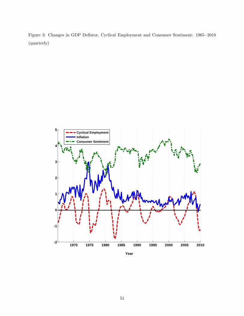
Figure 3: Changes in GDP Deflator, Cyclical Employment and Consumer Sentiment: 1965 - 2010

(quarterly)

1970 1975 1980 1985 1990 1995 2000 2005 2010-2

-1

0

1

2

3

4

5

Year

Cyclical Employment

Inflation

Consumer Sentiment

51

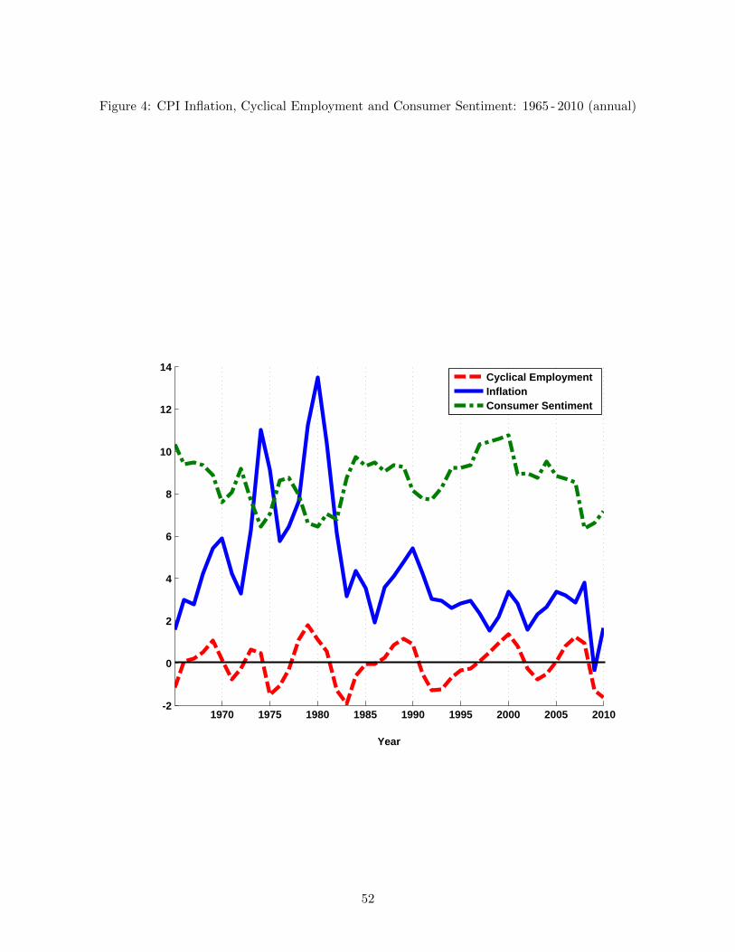
Figure 4: CPI Inflation, Cyclical Employment and Consumer Sentiment: 1965 - 2010 (annual)

1970 1975 1980 1985 1990 1995 2000 2005 2010-2

0

2

4

6

8

10

12

14

Year

Cyclical EmploymentInflationConsumer Sentiment

52

Figure 5: Impulse responses to a positive expectational shock for rule 1 with φy = 0.5

0 5 10 150

2

4

6

8x 10

-3 Producer Exp.

0 5 10 150

2

4

6

8x 10

-3 Consumer Exp.

0 5 10 150

2

4

6x 10

-3 Output

0 5 10 150

2

4

6x 10

-3 Hours

0 5 10 15-8

-6

-4

-2

0x 10

-3 Labor Wedge

0 5 10 15-1.5

-1

-0.5

0x 10

-4 Inflation

0 5 10 15-1

-0.5

0

0.5

1Expected Inflation

0 5 10 150

1

2

3x 10

-3 Nominal Rate

0 5 10 150

1

2

3x 10

-3 Real Rate

53

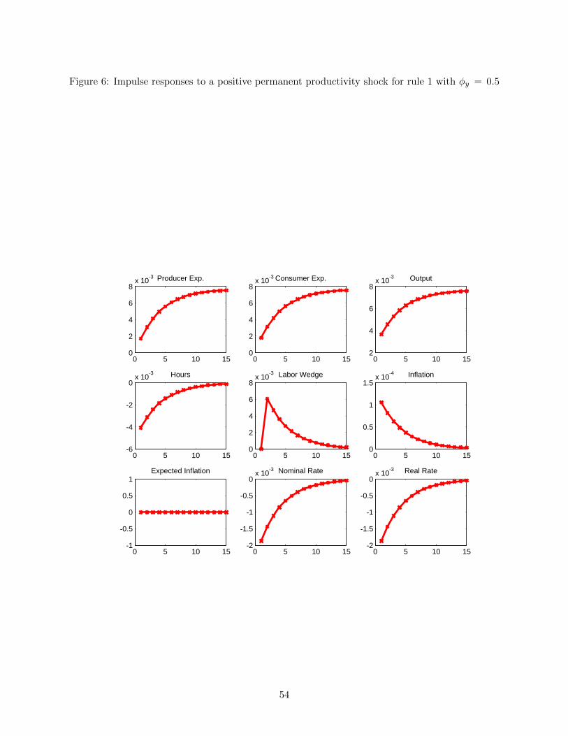
Figure 6: Impulse responses to a positive permanent productivity shock for rule 1 with φy = 0.5

0 5 10 150

2

4

6

8x 10

-3 Producer Exp.

0 5 10 150

2

4

6

8x 10

-3 Consumer Exp.

0 5 10 152

4

6

8x 10

-3 Output

0 5 10 15-6

-4

-2

0x 10

-3 Hours

0 5 10 150

2

4

6

8x 10

-3 Labor Wedge

0 5 10 150

0.5

1

1.5x 10

-4 Inflation

0 5 10 15-1

-0.5

0

0.5

1Expected Inflation

0 5 10 15-2

-1.5

-1

-0.5

0x 10

-3 Nominal Rate

0 5 10 15-2

-1.5

-1

-0.5

0x 10

-3 Real Rate

54

Figure 7: Impulse responses to a positive temporary productivity shock for rule 1 with φy = 0.5

0 5 10 150

0.5

1

1.5x 10

-3 Producer Exp.

0 5 10 150

0.5

1

1.5x 10

-3 Consumer Exp.

0 5 10 150

0.02

0.04

0.06Output

0 5 10 15-0.15

-0.1

-0.05

0

0.05Hours

0 5 10 15-0.1

0

0.1

0.2

0.3Labor Wedge

0 5 10 15-1

0

1

2

3x 10

-3 Inflation

0 5 10 15-1

-0.5

0

0.5

1Expected Inflation

0 5 10 15-0.06

-0.04

-0.02

0

0.02Nominal Rate

0 5 10 15-0.06

-0.04

-0.02

0

0.02Real Rate

55

Figure 8: Impulse responses to a positive expectational shock for rule 1 with φy = 0

0 5 10 150

2

4

6

8x 10

-3 Producer Exp.

0 5 10 150

2

4

6

8x 10

-3 Consumer Exp.

0 5 10 150

1

2

3x 10

-3 Output

0 5 10 150

1

2

3x 10

-3 Hours

0 5 10 15-6

-4

-2

0x 10

-3 Labor Wedge

0 5 10 150

1

2

3x 10

-3 Inflation

0 5 10 15-1

-0.5

0

0.5

1Expected Inflation

0 5 10 150

1

2

3

4x 10

-3 Nominal Rate

0 5 10 150

1

2

3

4x 10

-3 Real Rate

56

Figure 9: Impulse responses to a positive permanent productivity shock for rule 1 with φy = 0

0 5 10 150

2

4

6

8x 10

-3 Producer Exp.

0 5 10 150

2

4

6

8x 10

-3 Consumer Exp.

0 5 10 155

6

7

8x 10

-3 Output

0 5 10 15-3

-2

-1

0x 10

-3 Hours

0 5 10 150

1

2

3

4x 10

-3 Labor Wedge

0 5 10 15-3

-2

-1

0x 10

-3 Inflation

0 5 10 15-1

-0.5

0

0.5

1Expected Inflation

0 5 10 15-4

-3

-2

-1

0x 10

-3 Nominal Rate

0 5 10 15-4

-3

-2

-1

0x 10

-3 Real Rate

57

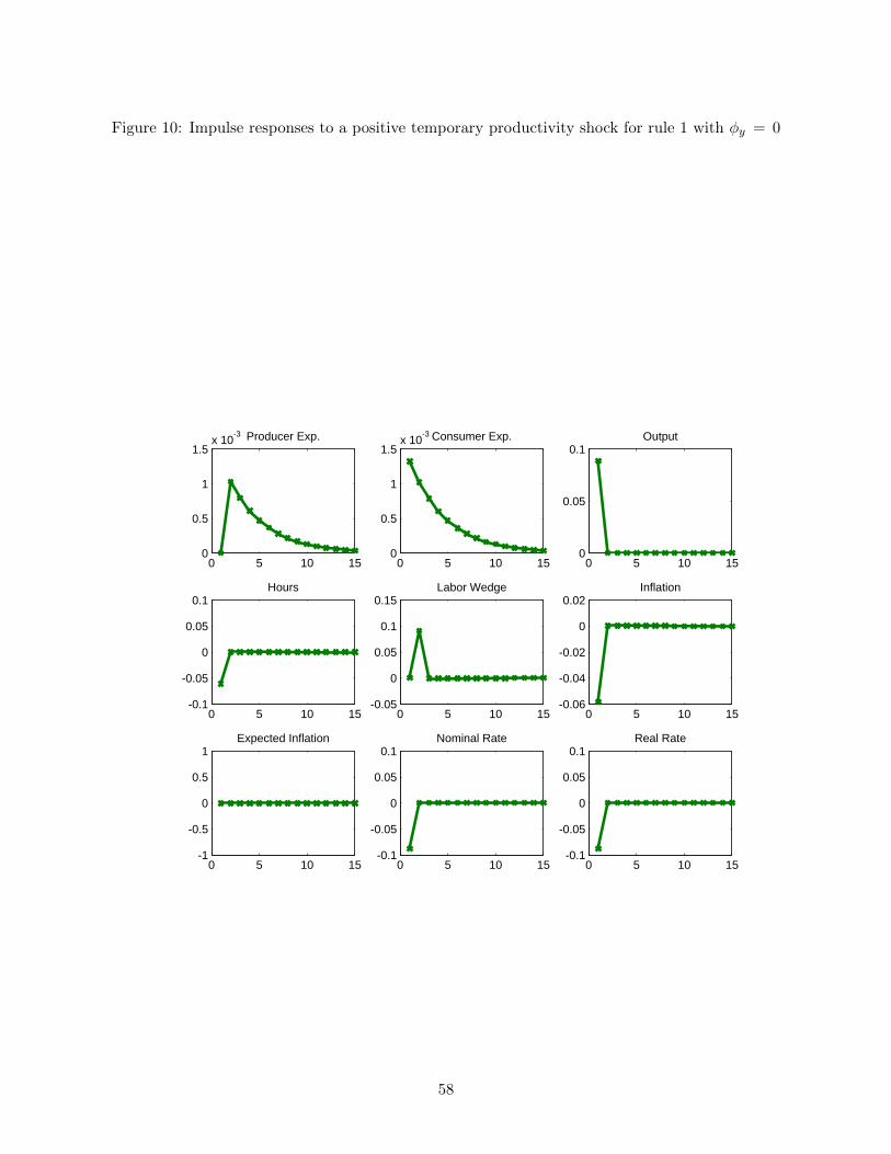
Figure 10: Impulse responses to a positive temporary productivity shock for rule 1 with φy = 0

0 5 10 150

0.5

1

1.5x 10

-3 Producer Exp.

0 5 10 150

0.5

1

1.5x 10

-3 Consumer Exp.

0 5 10 150

0.05

0.1Output

0 5 10 15-0.1

-0.05

0

0.05

0.1Hours

0 5 10 15-0.05

0

0.05

0.1

0.15Labor Wedge

0 5 10 15-0.06

-0.04

-0.02

0

0.02Inflation

0 5 10 15-1

-0.5

0

0.5

1Expected Inflation

0 5 10 15-0.1

-0.05

0

0.05

0.1Nominal Rate

0 5 10 15-0.1

-0.05

0

0.05

0.1Real Rate

58

Figure 11: Impulse responses to a positive expectational shock for baseline rule 2 (1)

0 5 10 150

1

2

3

4

5

6

7x 10

-3 Producer Expectations

0 5 10 150

1

2

3

4

5

6x 10

-3 Output

0 5 10 150

1

2

3

4

5

6x 10

-3 Hours

0 5 10 15-0.01

-0.008

-0.006

-0.004

-0.002

0Labor Wedge

59

Figure 12: Impulse responses to a positive expectational shock for baseline rule 2 (2)

0 5 10 150

0.005

0.01

0.015Price Levels

0 5 10 15-5

0

5

10

15x 10

-3 Inflation

0 5 10 150

2

4

6

8x 10

-3 Consumer Expectations

0 5 10 150

0.5

1

1.5

2x 10

-3 Expected Inflation

0 5 10 150

1

2

3x 10

-3 Nominal Interest Rate

0 5 10 150

0.5

1x 10

-3 Real Interest Rate

60

Figure 13: Impulse responses to a positive permanent productivity shock for baseline rule 2 (1)

0 5 10 151

2

3

4

5

6

7

8x 10

-3 Producer Expectations

0 5 10 152

3

4

5

6

7

8x 10

-3 Output

0 5 10 15-6

-5

-4

-3

-2

-1

0x 10

-3 Hours

0 5 10 150

2

4

6

8x 10

-3 Labor Wedge

61

Figure 14: Impulse responses to a positive permanent productivity shock for baseline rule 2 (2)

0 5 10 150.005

0.01

0.015

0.02Price Levels

0 5 10 150

2

4

6x 10

-3 Inflation

0 5 10 150

2

4

6

8x 10

-3 Consumer Expectations

0 5 10 15-2

-1.5

-1

-0.5

0x 10

-3 Expected Inflation

0 5 10 15-3

-2

-1

0x 10

-3 Nominal Interest Rate

0 5 10 15-1

-0.5

0x 10

-3 Real Interest Rate

62

Figure 15: Impulse responses to a positive temporary productivity shock for baseline rule 2 (1)

0 5 10 150

0.2

0.4

0.6

0.8

1

1.2x 10

-3 Producer Expectations

0 5 10 150

0.005

0.01

0.015

0.02

0.025Output

0 5 10 15-0.15

-0.1

-0.05

0

0.05Hours

0 5 10 15-0.05

0

0.05

0.1

0.15

0.2Labor Wedge

63

Figure 16: Impulse responses to a positive temporary productivity shock for baseline rule 2 (2)

0 5 10 150

0.02

0.04

0.06Price Levels

0 5 10 15-0.05

0

0.05Inflation

0 5 10 150

0.5

1

1.5x 10

-3 Consumer Expectations

0 5 10 15-0.06

-0.04

-0.02

0

0.02Expected Inflation

0 5 10 15-0.1

-0.05

0

0.05

0.1Nominal Interest Rate

0 5 10 15-0.03

-0.02

-0.01

0

0.01Real Interest Rate

64