washington university - galprop: home · to the washington university department of physics ... de...
TRANSCRIPT

WASHINGTON UNIVERSITY
Department of Physics
Dissertation Examination Committee:Martin H. Israel, Chair
W. Robert BinnsJames H. BuckleyRamanath Cowsik
Henric KrawczynskiWilliam B. McKinnon
Roger J. Phillips
COSMIC-RAY ENERGY LOSS IN THE HELIOSPHERE AND INTERSTELLAR
REACCELERATION
by
Lauren M. Scott
A dissertation presented to theGraduate School of Arts and Sciences
of Washington University inpartial fulfillment of the
requirements for the degreeof Doctor of Philosophy
August 2005
Saint Louis, Missouri
c©Copyright 2005by
Lauren M. Scott

For my parents:the original Drs. Scott

Acknowledgements
I am grateful to many people, both in and out of the workplace, for the valuable
guidance, advice and relief of graduate-student-related tension over the past six years.
These St. Louis years have been the best of my short life so far.
To the Washington University Department of Physics
I am eternally grateful to my thesis advisors, Drs. Marty Israel and Bob Binns, for
teaching me all about cosmic-ray physics, answering all my questions and providing
continuous support. To Marty, thanks for all the one-on-one conversations - it was
during those that I learned the most; your devotion to both teaching and research
inspires me. To Bob, thanks for your expertise and guidance during all of our work
out in the field; your focus and problem-solving skills under pressure have been an
inspiration to me. Special thanks also to Jim Buckley, Ramanath Cowsik, Michael
Friedlander, Paul Hink, Joe Klarmann, and Henric Krawczynski for teaching and
supporting me.
To our electrical engineer, Paul Dowkontt, thanks for keeping me on my toes and
teaching me the ins and outs of pulse-height analysis, and of course, for being the guy
iv
I could always count on to go get a beer out in the field. To our programmer Marty
Olevitch, thanks for teaching me all about C/C++ and for being my biggest beat-box
fan. To our mechanical engineer, John “Poppy” Epstein, thanks for teaching me how
to build a particle detector, and of course, for being the best Antarctic tent-mate ever.
To our electrical technician, Garry Simburger, thanks for your work ethic and skill in
the lab, and for all the support, laughs and “You gotta be kidding me”s out in the
field. To our mechanical technician, Dana Braun, thanks for your skill and attention
to detail, and for all those Antarctic “sure, sure, sure”s. To the machine shop guys,
Todd Hardt, Denny Huelsman, and Tony Biondo, thanks for all your tireless work
during the TIGER-building months.
Special thanks to my graduate-student friends and colleagues, Richard “Dicky”
Bose, Caleb Browning, Trey Garson, Allyson Gibson, Kris Gutierrez, Van Huett,
Scott Hughes, Mead Jordan, Karl Kosack, Kelly Lave, Vicky Lee, Jason Link, Su-
san Niebur, Jeremy Perkins, Stephanie Posdamer, Brian Rauch, Paul Rebillot, and
Randy Wolfmeyer.
To the ACE/CRIS collaboration
I offer my most sincere gratitude to the members of the ACE/CRIS collaboration
at the Goddard Space Flight Center and the California Institute of Technology:
Eric Christian, Christina Cohen, Alan Cummings, Andrew Davis, Jeff George, Alan
Labrador, Rick Leske, Dick Mewaldt, Ryan Ogliore, Luke Sollitt, Ed Stone, Tycho
von Rosenvinge and Nathan Yanasak. Special thanks to Mark Wiedenbeck for sup-
v

plementing my work with leaky-box cosmic-ray propagation models and to Georgia
de Nolfo for help with the GALPROP code.
In addition to the collaboration, special thanks to Igor Moskalenko and Andrew
Strong for the use of and help with the GALPROP code and to the NASA Graduate
Student Researcher’s Program for funding my work.
To my family
Thanks to my parents, Ginny and Rick, for being with me in every way that parents
can. You taught me how to be. I am forever grateful for your influence on me aca-
demically and otherwise. To my brother, Ian, thanks for keeping me real, supporting
me and being the best big little brother. Your beautiful outlook on life helps me to
realize what things are the most important. And to the rest of my crazy collection
of a family: Gay, Susie, Jesi, Liz, Chris, Josh, Susannah, Libby, David and Jordan
thanks for always making life exciting and new.
To the funhounds
It is you without whom none of this would be possible. Huge thanks to my best
friend and roommate, Aaron Hock, for being my confidante, my yes-man and my
boy-wife and to Jen Banks for improving the quality of life through laughter, Jager
and invitations to the sanctuary. Special thanks to my dearest friends in and out
of the department: Paul, for the support and advice, and of course for the dollar
pitchers and late-night 100.3 The Beat; Karl, for your support and always being the
vi
go-to guy for my irritating computing questions, and of course for your refrigerator
tipping skills and ventures to l’Eglise de Poulet; Dicky, for being my peep and for
all those post-business trip lunches in the Loop; Jamie Eikmeier, for letting me play
piano at your wedding and always making me laugh.
Special thanks to: Don Carlos, the Crowbar, Brad Davis, Mel Eisner, Ryan Hale,
Blueberry Hill, Kristin Huml, Jem and the Holograms, Nihal Joag, Karaoke, Gabi
Koch, Will Lamb, Colin Leary, Beth Leonhardt, Anna MacKay, Rose Martelli, Nelly,
Donna Perkins, Mariana Pickering, Allyson Pilat, “Boy” Aaron Powell, Amber Pow-
ers, Dave Schneider, E. H. Schnuck, Ali Stritzl, Kent Towers, Vess, Danette Wilson,
Gretchen Wolfmeyer, Ellen Wurm and the neighbor who unwittingly provided me
with free wireless internet at home during the thesis-writing months.
And finally to my love
Leah Owens, for loving and supporting me. Your intelligence, your wit and your free
spirit inspires me. Here’s to you and me and the next chapter of life.
vii

Contents
Copyright ii
Dedication iii
Acknowledgements iv
List of Figures xiv
List of Tables xv
Abstract xvi
1 Introduction 11.1 Galactic Cosmic Rays . . . . . . . . . . . . . . . . . . . . . . . . . . . 1
1.1.1 History . . . . . . . . . . . . . . . . . . . . . . . . . . . . . . . 21.1.2 Source and acceleration . . . . . . . . . . . . . . . . . . . . . . 41.1.3 Propagation and reacceleration . . . . . . . . . . . . . . . . . 11
1.2 Cosmic Rays in the heliosphere . . . . . . . . . . . . . . . . . . . . . 131.2.1 The 22-year solar cycle . . . . . . . . . . . . . . . . . . . . . . 131.2.2 Particle transport in the heliosphere . . . . . . . . . . . . . . . 151.2.3 Diffusion, convection and adiabatic energy loss . . . . . . . . . 171.2.4 This solar modulation model . . . . . . . . . . . . . . . . . . . 18
1.3 Detection . . . . . . . . . . . . . . . . . . . . . . . . . . . . . . . . . 191.3.1 Advanced Composition Explorer . . . . . . . . . . . . . . . . . 211.3.2 Trans-Iron Galactic Element Recorder . . . . . . . . . . . . . 221.3.3 Other Galactic cosmic ray detectors . . . . . . . . . . . . . . . 25
1.4 Scope of this work . . . . . . . . . . . . . . . . . . . . . . . . . . . . 31
2 Cosmic Ray Isotope Spectrometer 322.1 Scintillating Optical Fiber Trajectory system . . . . . . . . . . . . . . 342.2 Silicon stack detector system . . . . . . . . . . . . . . . . . . . . . . . 352.3 CRIS inflight data output . . . . . . . . . . . . . . . . . . . . . . . . 36
2.3.1 Event data . . . . . . . . . . . . . . . . . . . . . . . . . . . . . 362.3.2 Housekeeping and rate data . . . . . . . . . . . . . . . . . . . 37
2.4 The dEdx
· E technique . . . . . . . . . . . . . . . . . . . . . . . . . . . 37
viii

Contents
3 Data Analysis 403.1 Selecting usable data with xpick . . . . . . . . . . . . . . . . . . . . 41
3.1.1 Preliminary exclusion criteria . . . . . . . . . . . . . . . . . . 413.1.2 Charge consistency . . . . . . . . . . . . . . . . . . . . . . . . 423.1.3 Mass calculation . . . . . . . . . . . . . . . . . . . . . . . . . 433.1.4 Depth calculation . . . . . . . . . . . . . . . . . . . . . . . . . 433.1.5 Geometrical cuts and mass avg corrections . . . . . . . . . . . 443.1.6 Temporal cuts . . . . . . . . . . . . . . . . . . . . . . . . . . . 483.1.7 Angle cuts . . . . . . . . . . . . . . . . . . . . . . . . . . . . . 50
3.2 The Dataset . . . . . . . . . . . . . . . . . . . . . . . . . . . . . . . . 513.2.1 Delineating time intervals . . . . . . . . . . . . . . . . . . . . 513.2.2 Mass histograms . . . . . . . . . . . . . . . . . . . . . . . . . 51
3.3 Histogram plots for solar minimum data . . . . . . . . . . . . . . . . 533.3.1 B histograms . . . . . . . . . . . . . . . . . . . . . . . . . . . 543.3.2 C histograms . . . . . . . . . . . . . . . . . . . . . . . . . . . 553.3.3 N histograms . . . . . . . . . . . . . . . . . . . . . . . . . . . 563.3.4 O histograms . . . . . . . . . . . . . . . . . . . . . . . . . . . 573.3.5 F histograms . . . . . . . . . . . . . . . . . . . . . . . . . . . 583.3.6 Ne histograms . . . . . . . . . . . . . . . . . . . . . . . . . . . 593.3.7 Na histograms . . . . . . . . . . . . . . . . . . . . . . . . . . . 603.3.8 Mg histograms . . . . . . . . . . . . . . . . . . . . . . . . . . 613.3.9 Al histograms . . . . . . . . . . . . . . . . . . . . . . . . . . . 623.3.10 Si histograms . . . . . . . . . . . . . . . . . . . . . . . . . . . 633.3.11 P histograms . . . . . . . . . . . . . . . . . . . . . . . . . . . 643.3.12 S histograms . . . . . . . . . . . . . . . . . . . . . . . . . . . 653.3.13 Cl histograms . . . . . . . . . . . . . . . . . . . . . . . . . . . 663.3.14 Ar histograms . . . . . . . . . . . . . . . . . . . . . . . . . . . 673.3.15 K histograms . . . . . . . . . . . . . . . . . . . . . . . . . . . 683.3.16 Ca histograms . . . . . . . . . . . . . . . . . . . . . . . . . . . 693.3.17 Sc histograms . . . . . . . . . . . . . . . . . . . . . . . . . . . 703.3.18 Ti histograms . . . . . . . . . . . . . . . . . . . . . . . . . . . 713.3.19 V histograms . . . . . . . . . . . . . . . . . . . . . . . . . . . 723.3.20 Cr histograms . . . . . . . . . . . . . . . . . . . . . . . . . . . 733.3.21 Mn histograms . . . . . . . . . . . . . . . . . . . . . . . . . . 743.3.22 Fe histograms . . . . . . . . . . . . . . . . . . . . . . . . . . . 753.3.23 Co histograms . . . . . . . . . . . . . . . . . . . . . . . . . . . 763.3.24 Ni histograms . . . . . . . . . . . . . . . . . . . . . . . . . . . 77
3.4 Fragmentation corrections . . . . . . . . . . . . . . . . . . . . . . . . 783.5 SOFT Efficiency corrections . . . . . . . . . . . . . . . . . . . . . . . 793.6 Abundance ratios . . . . . . . . . . . . . . . . . . . . . . . . . . . . . 803.7 Spectral calculations . . . . . . . . . . . . . . . . . . . . . . . . . . . 81
ix

Contents
4 CRIS Measurements of Electron-Capture-Decay Isotopes 824.1 Electron-capture decay . . . . . . . . . . . . . . . . . . . . . . . . . . 824.2 Electron-capture decay in GCRs . . . . . . . . . . . . . . . . . . . . . 84
4.2.1 Electron attachment . . . . . . . . . . . . . . . . . . . . . . . 844.2.2 Electron stripping . . . . . . . . . . . . . . . . . . . . . . . . . 85
4.3 CRIS observations of electron-capture decay . . . . . . . . . . . . . . 864.3.1 37Ar → 37Cl . . . . . . . . . . . . . . . . . . . . . . . . . . . . 914.3.2 41Ca → 41K . . . . . . . . . . . . . . . . . . . . . . . . . . . . 944.3.3 44Ti → 44Sc → 44Ca . . . . . . . . . . . . . . . . . . . . . . . 974.3.4 49V → 49Ti . . . . . . . . . . . . . . . . . . . . . . . . . . . . 1004.3.5 51Cr → 51V . . . . . . . . . . . . . . . . . . . . . . . . . . . . 1034.3.6 53Mn → 53Cr . . . . . . . . . . . . . . . . . . . . . . . . . . . 1064.3.7 54Mn → 54Cr . . . . . . . . . . . . . . . . . . . . . . . . . . . 1094.3.8 55Fe → 55Mn . . . . . . . . . . . . . . . . . . . . . . . . . . . 1124.3.9 57Co → 57Fe . . . . . . . . . . . . . . . . . . . . . . . . . . . 115
4.4 Summary of observations . . . . . . . . . . . . . . . . . . . . . . . . . 118
5 Comparison of CRIS data with a Leaky-Box model 1205.1 The Leaky-Box model . . . . . . . . . . . . . . . . . . . . . . . . . . 1205.2 Comparison with EC decay abundance ratios . . . . . . . . . . . . . . 124
5.2.1 37Ar → 37Cl . . . . . . . . . . . . . . . . . . . . . . . . . . . . 1255.2.2 44Ti → 44Ca . . . . . . . . . . . . . . . . . . . . . . . . . . . 1295.2.3 49V → 49Ti . . . . . . . . . . . . . . . . . . . . . . . . . . . . 1325.2.4 51Cr → 51V . . . . . . . . . . . . . . . . . . . . . . . . . . . . 1375.2.5 55Fe → 55Mn . . . . . . . . . . . . . . . . . . . . . . . . . . . 142
5.3 Parameterizing solar modulation . . . . . . . . . . . . . . . . . . . . . 145
6 Probing reacceleration with the GALPROP propagation model 1486.1 Reacceleration in electron-capture decay secondaries . . . . . . . . . . 1486.2 The GALPROP code . . . . . . . . . . . . . . . . . . . . . . . . . . . . 1496.3 Three GALPROP models . . . . . . . . . . . . . . . . . . . . . . . . . . 152
6.3.1 Plain Diffusion model . . . . . . . . . . . . . . . . . . . . . . . 1526.3.2 Diffusive Reacceleration model . . . . . . . . . . . . . . . . . . 1586.3.3 Diffusion / Convection with Minimal Reacceleration . . . . . . 161
6.4 Summary of comparisons with GALPROP . . . . . . . . . . . . . . . . . 167
7 Conclusions 1737.1 Improvements on the analysis methods . . . . . . . . . . . . . . . . . 1737.2 Direct evidence of cosmic-ray energy loss in the heliosphere . . . . . . 1747.3 No evidence of reacceleration . . . . . . . . . . . . . . . . . . . . . . . 175
Bibliography 176
x

Contents
A The Maximum-Likelihood multiple-Gaussian fitting technique 183A.1 The Least-Squares method . . . . . . . . . . . . . . . . . . . . . . . . 183A.2 The Maximum-Likelihood method . . . . . . . . . . . . . . . . . . . . 184A.3 Calculating Uncertainties . . . . . . . . . . . . . . . . . . . . . . . . . 185A.4 Uncorrelated Uncertainties . . . . . . . . . . . . . . . . . . . . . . . . 185A.5 Correlated Uncertainties . . . . . . . . . . . . . . . . . . . . . . . . . 186
A.5.1 Diagonal Components . . . . . . . . . . . . . . . . . . . . . . 187A.5.2 Off-Diagonal Components . . . . . . . . . . . . . . . . . . . . 187
A.6 The Fitting Routine . . . . . . . . . . . . . . . . . . . . . . . . . . . 188
B Range-energy and spectral adjustments to isotopic ratios 203B.1 A necessity for the CRIS instrument . . . . . . . . . . . . . . . . . . 203B.2 Spectral shape . . . . . . . . . . . . . . . . . . . . . . . . . . . . . . . 204B.3 Range-energy relation . . . . . . . . . . . . . . . . . . . . . . . . . . . 204B.4 Adjusting an isotopic abundance . . . . . . . . . . . . . . . . . . . . 205
C Geometry Factor 208C.1 The Monte-Carlo technique . . . . . . . . . . . . . . . . . . . . . . . 208C.2 Determining the geometry factor and energy . . . . . . . . . . . . . . 211
D Isotopic Spectra 215
xi

List of Figures
1.1 GCR vs. Solar System elemental abundances . . . . . . . . . . . . . . 51.2 Total flux of all cosmic rays . . . . . . . . . . . . . . . . . . . . . . . 71.3 Abundances of GCRs with 30 ≤ Z ≤ 40 . . . . . . . . . . . . . . . . 101.4 Climax Neutron Monitor Count Rate . . . . . . . . . . . . . . . . . . 161.5 ACE spacecraft breakout . . . . . . . . . . . . . . . . . . . . . . . . . 231.6 Charge histogram of TIGER data . . . . . . . . . . . . . . . . . . . . 24
2.1 Inside the CRIS instrument . . . . . . . . . . . . . . . . . . . . . . . 322.2 CRIS schematic (top view) . . . . . . . . . . . . . . . . . . . . . . . . 332.3 CRIS schematic (side view) . . . . . . . . . . . . . . . . . . . . . . . 342.4 (E1+E2)cos(θ) vs. E3 charge bands . . . . . . . . . . . . . . . . . . . 38
3.1 Non-linearities in rp proj vs mass avg . . . . . . . . . . . . . . . . . 453.2 Adjusting mass avg for rp proj dependencies . . . . . . . . . . . . . 483.3 Instrument / Solar Event Dead Time . . . . . . . . . . . . . . . . . . 493.4 V histograms at 20, 30, and 45 . . . . . . . . . . . . . . . . . . . . 503.5 27-day average intensity of 16O, 28Si, and 56Fe over the ACE lifetime . 523.6 B mass histograms at solar minimum . . . . . . . . . . . . . . . . . . 543.7 C mass histograms at solar minimum . . . . . . . . . . . . . . . . . . 553.8 N mass histograms at solar minimum . . . . . . . . . . . . . . . . . . 563.9 O mass histograms at solar minimum . . . . . . . . . . . . . . . . . . 573.10 F mass histograms at solar minimum . . . . . . . . . . . . . . . . . . 583.11 Ne mass histograms at solar minimum . . . . . . . . . . . . . . . . . 593.12 Na mass histograms at solar minimum . . . . . . . . . . . . . . . . . 603.13 Mg mass histograms at solar minimum . . . . . . . . . . . . . . . . . 613.14 Al mass histograms at solar minimum . . . . . . . . . . . . . . . . . . 623.15 Si mass histograms at solar minimum . . . . . . . . . . . . . . . . . . 633.16 P mass histograms at solar minimum . . . . . . . . . . . . . . . . . . 643.17 S mass histograms at solar minimum . . . . . . . . . . . . . . . . . . 653.18 Cl mass histograms at solar minimum . . . . . . . . . . . . . . . . . . 663.19 Ar mass histograms at solar minimum . . . . . . . . . . . . . . . . . 673.20 K mass histograms at solar minimum . . . . . . . . . . . . . . . . . . 683.21 Ca mass histograms at solar minimum . . . . . . . . . . . . . . . . . 693.22 Sc mass histograms at solar minimum . . . . . . . . . . . . . . . . . . 70
xii

List of Figures
3.23 Ti mass histograms at solar minimum . . . . . . . . . . . . . . . . . . 713.24 V mass histograms at solar minimum . . . . . . . . . . . . . . . . . . 723.25 Cr mass histograms at solar minimum . . . . . . . . . . . . . . . . . 733.26 Mn mass histograms at solar minimum . . . . . . . . . . . . . . . . . 743.27 Fe mass histograms at solar minimum . . . . . . . . . . . . . . . . . . 753.28 Co mass histograms at solar minimum . . . . . . . . . . . . . . . . . 763.29 Ni mass histograms at solar minimum . . . . . . . . . . . . . . . . . . 77
4.1 The time scales of various processes for EC decay isotopes . . . . . . 874.2 Modeling 51V/51Cr with and without EC decay . . . . . . . . . . . . 884.3 37Cl/37Ar at solar minimum and maximum . . . . . . . . . . . . . . . 934.4 Ca mass histograms at solar minimum and maximum, θ < 30 . . . . 964.5 41K/41Ca at solar minimum and maximum . . . . . . . . . . . . . . . 964.6 44Ca/44Ti at solar minimum and maximum . . . . . . . . . . . . . . . 994.7 49Ti/49V at solar minimum and maximum . . . . . . . . . . . . . . . 1024.8 51V/51Cr at solar minimum and maximum . . . . . . . . . . . . . . . 1054.9 53Cr/53Mn at solar minimum and maximum . . . . . . . . . . . . . . 1084.10 54Cr/54Mn at solar minimum and maximum . . . . . . . . . . . . . . 1114.11 Fe mass histograms at solar minimum and maximum, θ < 25 . . . . 1144.12 55Mn/55Fe at solar minimum and maximum . . . . . . . . . . . . . . 1144.13 57Fe/57Co at solar minimum and maximum . . . . . . . . . . . . . . . 117
5.1 (Sc+Ti+V)/Fe at solar minimum with LBM predictions . . . . . . . 1225.2 37Cl/37Ar at solar minimum with LBM predictions . . . . . . . . . . 1255.3 Measured total production cross sections for 37Ar and 37Cl . . . . . . 1265.4 Comparison of 37Cl/40Ca and 37Ar/40Ar to LBM . . . . . . . . . . . . 1275.5 44Ca/44Ti at solar minimum with LBM predictions . . . . . . . . . . 1295.6 Measured total production cross sections for 44Ti and 44Ca . . . . . . 1305.7 Comparison of 44Ti/56Fe and 44Ca/56Fe to LBM . . . . . . . . . . . . 1315.8 Measured total production cross sections for 49V and 49Ti . . . . . . . 1335.9 Comparison of 49V to 50Cr, 52Cr, 55Mn, 54Fe, 56Fe to LBM . . . . . . 1345.10 Comparison of 49Ti to 52Cr, 55Mn 56Fe to LBM . . . . . . . . . . . . 1355.11 49Ti/49V at solar minimum and maximum with LBM predictions . . . 1365.12 Measured total production cross sections for 51Cr and 51V . . . . . . 1385.13 Comparison of 51Cr to 52Cr, 55Mn, 54Fe, 56Fe to LBM . . . . . . . . . 1395.14 Comparison of 51V to 52Cr, 55Mn, 56Fe to LBM . . . . . . . . . . . . 1405.15 51V/51Cr at solar minimum and maximum with LBM predictions . . 1415.16 55Mn/55Fe at solar minimum and maximum with LBM predictions . . 1425.17 Measured total production cross sections for 55Fe and 55Mn . . . . . . 1435.18 Comparison of 55Fe/56Fe, 55Fe/58Ni, 55Mn/56Fe to LBM . . . . . . . . 1445.19 χ2 fits for 49Ti/49V and 51V/51Cr to modulated LBM predictions . . . 1465.20 Inferred φ from spectral fits of C, O, Mg, Si and Fe . . . . . . . . . . 147
6.1 B/C and (Sc+Ti+V)/Fe with GALPROP PD . . . . . . . . . . . . . . . 153
xiii

List of Figures
6.2 49Ti/49V and 51V/51Cr with GALPROP PD . . . . . . . . . . . . . . . . 1546.3 49Ti and 49V in the context of GALPROP PD . . . . . . . . . . . . . . . 1566.4 51V and 51Cr in the context of GALPROP PD . . . . . . . . . . . . . . 1576.5 B/C and (Sc+Ti+V)/Fe with GALPROP DR . . . . . . . . . . . . . . . 1596.6 49Ti/49V and 51V/51Cr with GALPROP DR . . . . . . . . . . . . . . . . 1616.7 49Ti and 49V in the context of GALPROP DR . . . . . . . . . . . . . . . 1626.8 51V and 51Cr in the context of GALPROP DR . . . . . . . . . . . . . . 1636.9 B/C and (Sc+Ti+V)/Fe GALPROP DCMR . . . . . . . . . . . . . . . 1656.10 B/C and (Sc+Ti+V)/Fe with GALPROP “wave-damped” DCMR . . . 1656.11 49Ti/49V and 51V/51Cr with GALPROP “wave-damped” DCMR . . . . 1676.12 49Ti and 49V in the context of GALPROP “wave-damped” DCMR . . . 1686.13 51V and 51Cr in the context of GALPROP “wave-damped” DCMR . . . 1696.14 Best-fit φ for data, LBM and GALPROP during solar minimum . . . . . 171
A.1 Representation of maximum-likelihood uncorrelated errors . . . . . . 186A.2 Representation of maximum-likelihood correlated errors . . . . . . . . 188
B.1 Spectral/Range-energy adjustment of 51Cr to 51V . . . . . . . . . . . 205
C.1 Geometry Factor Monte Carlo simulation . . . . . . . . . . . . . . . . 209C.2 Geometry Factor for 56Fe, θ < 30 . . . . . . . . . . . . . . . . . . . . 210C.3 56Fe bowtie diagrams . . . . . . . . . . . . . . . . . . . . . . . . . . . 213
D.1 Isotopic Spectra (B to F) . . . . . . . . . . . . . . . . . . . . . . . . . 215D.2 Isotopic Spectra (Ne to Ar) . . . . . . . . . . . . . . . . . . . . . . . 216D.3 Isotopic Spectra (K to Cr . . . . . . . . . . . . . . . . . . . . . . . . 217D.4 Isotopic Spectra (Mn to Ni) . . . . . . . . . . . . . . . . . . . . . . . 218
xiv

List of Tables
3.1 Dead-layer cuts on rp proj . . . . . . . . . . . . . . . . . . . . . . . . 46
4.1 Electron-capture decay isotopes and their decay half-lives . . . . . . . 834.2 CRIS 37Ar and 37Cl measurements . . . . . . . . . . . . . . . . . . . 924.3 CRIS 37Ar/37Cl at solar minimum and solar maximum . . . . . . . . 934.4 CRIS 41Ca and 41K measurements . . . . . . . . . . . . . . . . . . . . 954.5 CRIS 41K/41Ca at solar minimum and solar maximum . . . . . . . . 964.6 CRIS 44Ti and 44Ca measurements . . . . . . . . . . . . . . . . . . . 984.7 CRIS 44Ti/44Ca at solar minimum and solar maximum . . . . . . . . 994.8 CRIS 49V and 49Ti measurements . . . . . . . . . . . . . . . . . . . . 1014.9 CRIS 49V/49Ti at solar minimum and solar maximum . . . . . . . . . 1024.10 CRIS 51Cr and 51V measurements . . . . . . . . . . . . . . . . . . . . 1044.11 CRIS 51Cr/51V at solar minimum and solar maximum . . . . . . . . . 1054.12 CRIS 53Mn and 53Cr measurements . . . . . . . . . . . . . . . . . . . 1074.13 CRIS 53Cr/53Mn at solar minimum and solar maximum . . . . . . . . 1084.14 CRIS 54Mn and 54Cr measurements . . . . . . . . . . . . . . . . . . . 1104.15 CRIS 54Cr/54Mn at solar minimum and solar maximum . . . . . . . . 1114.16 CRIS 55Fe and 55Mn measurements . . . . . . . . . . . . . . . . . . . 1134.17 CRIS 55Fe/55Mn at solar minimum and solar maximum . . . . . . . . 1144.18 CRIS 57Co and 57Fe measurements . . . . . . . . . . . . . . . . . . . 1164.19 CRIS 57Co/57Fe at solar minimum and solar maximum . . . . . . . . 117
5.1 Observed φ at solar minimum and solar maximum . . . . . . . . . . . 145
6.1 Parameters for GALPROP PD Model . . . . . . . . . . . . . . . . . . . 1526.2 Parameters for GALPROP DR Model . . . . . . . . . . . . . . . . . . . 1586.3 Parameters for GALPROP DCMR model . . . . . . . . . . . . . . . . . 1616.4 Observed φ for three GALPROP models . . . . . . . . . . . . . . . . . . 170
B.1 Range-energy (R = kAZ2E
α) fits for selected isotopes . . . . . . . . . . 207
xv

Abstract
Using data collected by the Cosmic Ray Isotope Spectrometer (CRIS) on the NASA
Advanced Composition Explorer (ACE ) spacecraft, I report on measurements of
Galactic Cosmic Ray isotopes in the energy range from 50 to 550 MeV/nucleon,
with emphasis on the electron-capture-decay secondaries, 37Cl, 41Ca, 44Ti, 49V, 51Cr,
55Fe and 57Co. These isotopes, which decay only by electron-capture are effectively
stable in the cosmic rays at high energies where electron attachment is unlikely; at
lower energies substantial electron attachment and decay does occur. By comparing
the daughter-to-parent abundance ratios 49Ti/49V and 51V/51Cr during periods of
solar minimum and solar maximum, I report new direct evidence of changes in the
amount of energy loss that occurs in cosmic rays between solar minimum and solar
maximum. Comparison of the electron-capture-decay abundance ratios with propa-
gation models in the context of reacceleration are also presented. Analysis shows that
little or no reacceleration is needed to correctly predict the energy-dependence of the
electron-capture abundance ratios.
xvi

Chapter 1
Introduction
1.1 Galactic Cosmic Rays
Galactic cosmic rays (GCRs) are atomic nuclei, electrons, positrons and anti-protons
of extra-solar origin that propagate at high energies in the interstellar medium. All
elements in the periodic table are present in the cosmic rays, 87% of which are pro-
tons, 12% He nuclei and approximately one percent of which are nuclei with Z > 2
(Longair, 1992). They range in energy from just a few tens of MeV per nucleon to
energies as high as ∼ 1020 eV, where it is expected that higher energies are prohibited
due to interactions with the 2.7 K cosmic microwave background, a phenomenon now
known as the Greisen-Zatsepin-Kuzmin (GZK) cutoff (Greisen, 1966). Cosmic rays
are isotropic in that they have no preferred arrival direction.
The study of GCRs permits us to come closer to answering questions involving
their source, mechanisms of acceleration and characteristics of propagation in the
interstellar medium. Perhaps to a greater degree, GCRs give insight into the pro-
cesses of stellar evolution, supernova explosions other high-energy phenomena in the
universe, as well as a better understanding of the effects of solar modulation.
1

1.1 Galactic Cosmic Rays
1.1.1 History
The study of galactic cosmic rays (GCRs) began with their discovery by Victor Hess
during his legendary 1912 balloon flight, an experiment for which he won the 1936
Nobel Prize in Physics. Hess observed with an electroscope that the intensity of
ionizing radiation increased with altitude, leading him to believe that the radiation
was extraterrestrial in origin.
The Nobel Laureate Robert Millikan, in an effort to test Hess’ hypothesis, con-
ducted several experiments to verify the extraterrestrial origin of these cosmic rays.
His first two experiments provided erroneous results. A meteorological balloon equipped
with automated detectors reached an altitude of 15 km and seemed to show prelimi-
narily that the radiation did not increase with altitude. The results were later deemed
unreliable due to severe temperature gradients in the instrumentation during flight.
During a second experiment conducted at Pike’s Peak, Millikan erroneously assumed
that a shielding material made of 4.8 cm of lead would be much less than the shielding
provided by the atmosphere above, and hence found there to be no excess in radia-
tion. A final experiment conducted at a mountain-top lake showed that the radiation
decreased with depth in the lake, thereby finally confirming Hess’ discovery.
The question of whether the observed radiation was caused by charged particles
or gamma rays was at the center of a controversy headed by Millikan, who believed
that the primary particles were gamma rays, and his former student Arthur Compton,
who believed that they were charged particles. An experiment conducted by Bothe
2

1.1 Galactic Cosmic Rays
and Kolhorster in 1929 began to unravel the mystery. Using two Geiger counters as
a coincidence system, they noted that the two discharged simultaneously quite often,
even when slabs of lead and gold were placed between them. Reasoning correctly that
it was highly unlikely for the secondary electrons produced by an incident gamma ray
to discharge the Geiger counters nearly simultaneously, their result was that the
cosmic rays observed near the ground were charged particles (Smith, 1996).
The first direct evidence that the primary particles incident on the earth’s atmo-
sphere were charged came during a latitude survey conducted by Compton in the early
1930s. Compton noticed that the amount of the observed radiation decreased toward
the equator and reasoned correctly that the earth’s magnetic field was responsible for
the deflection of the charged primary radiation (Compton, 1933).
The discovery of cosmic rays helped to usher in a new era of discovery on the
atomic and subatomic scale. In the 1930s, cosmic rays were used extensively in the
discovery of new particles. Expanding on the previous work of Millikan and Anderson,
Blackett and Occhialini in 1933 developed an apparatus consisting of a two-Geiger-
counter coincidence system similar to that used by Bothe and Kolhorster, a powerful
electromagnet, and a cloud chamber. Cosmic rays interacting with the body of the
apparatus permitted the first detailed images of electron tracks.
In 1936, using a similar method, Anderson and Neddermeyer imaged muon tracks
in a cloud chamber and made the first approximations to the mass of these particles,
intermediate to those of the electron and the proton. In the late 1940s, Rochester and
Butler used a similar procedure to discover the K+, K−, K0 and Λ particles. By the
3

1.1 Galactic Cosmic Rays
end of the 1940s, nuclear emulsions had paved the way to the discovery of the the π+
and π−, and the first three-dimensional imaging of their subsequent decay into muons
and then finally into electons and positrons. Into the 1950s, cosmic-ray studies had
assisted in the discovery of the Ξ− and the Σ (Longair, 1992).
Cosmic-ray astrophysics has since blossomed into one of the most important sci-
entific endeavors of the twentieth century. Along with refractory, pre-solar meteoritic
dust grains, cosmic rays provide the only means of directly gathering material from
outside our solar system. Some of the most important questions that remain unan-
swered involve defining the source and acceleration mechanisms of these high-energy
particles and what conditions they encounter as they propagate in the interstellar
medium. At a more rudimentary level, one of the most important concerns involves
being able to approximate the extent to which cosmic rays decrease in intensity and
lose energy as they propagate in the heliosphere.
1.1.2 Source and acceleration
Cosmic rays can be classified into three main groups: anomalous cosmic rays (ACRs),
galactic cosmic rays (GCRs) and extragalactic cosmic rays. Anomalous cosmic rays
are partially ionized nuclei that originate in neutral gas in the interstellar medium
(Pesses et al., 1981). They are stripped of one or more of their outer electrons and
become “pick up” ions in the heliosphere. They are then accelerated at the solar
wind termination shock and are normally found with energies ranging from a few to a
few tens of MeV/nucleon (Fisk et al., 1974). Galactic cosmic rays are totally ionized
4

1.1 Galactic Cosmic Rays
Figure 1.1: Relative elemental abundances with 1 ≤ Z ≤ 30 in the solar system andin the GCRs. Data for H and He from BESS and IMP-8 measurements. Data for3 ≤ Z ≤ 28 measured with the ACE/CRIS instrument. Data for Cu and Zn fromMurdin (2000). Note the enhancement in Li, Be, B (Z = 3, 4, 5) and the sub-Feelements Sc, Ti, V and Cr (Z = 21, 22, 23, and 24). Solar system abundances werederived from Lodders (2003).
nuclei that originate outside the solar system and can be observed with energies
ranging from ∼ 100 MeV/nucleon to energies in excess of 1019 eV. While most cosmic
rays are accelerated in areas within the Galaxy, those with energies above ∼ 1018 eV
are thought to be extragalactic in origin. This dissertation will only examine GCRs.
Atomic nuclei account for about 98% of GCRs, while the remaining 2% include
electrons, positrons and anti-protons. Galactic cosmic rays heavier than He are most
abundant in C, N, O, Ne, Mg, Si and Fe, with a significant decrease in intensity above
5

1.1 Galactic Cosmic Rays
Fe. Models show that nuclei heavier than Fe originate in both s- and r-process reac-
tions in red giant stars and in Type Ib, Ic and II supernova explosions, respectively.
Galactic cosmic rays can be classified either as primary nuclei, those that are pro-
duced at the source, accelerated, and detected at Earth, or secondary nuclei, which
are created by fragmentation of heavier nuclei in interactions with ambient gas in the
interstellar medium, most of which is hydrogen.
In most instances, the elemental abundances of the GCRs are in good agreement
with the corresponding solar system abundances, as measured from photospheric
and meteoritic data (Lodders, 2003). The most notable discrepancies can be seen in
Figure 1.1 and include the ∼ 105 enhancement in Li, Be and B in the GCRs over the
solar system abundances and the ∼ 102 − 104 enhancement in the sub-Fe elements,
Sc, Ti and V in the GCRs over the solar system abundances. These features are
widely known to be caused by the spallation of C, N, O (in the case of Li, Be and B)
and Fe (in the case of Sc, Ti and V) on ambient gas in the interstellar medium.
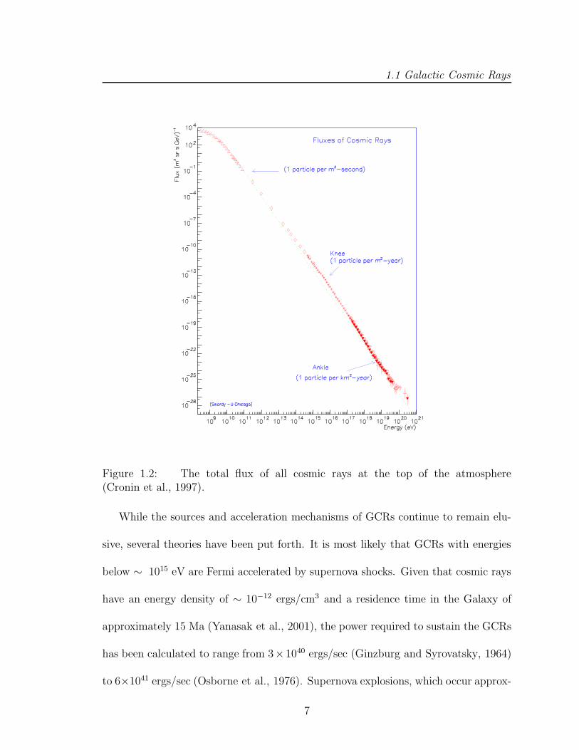
Galactic cosmic rays above a few hundred MeV/nucleon obey a power-law spec-
trum, falling as E−2.7 until ∼ 1015 eV (a feature commonly known as the “knee”) and
going as E−3.0 until ∼ 1018 eV. This feature in the spectrum, known as the “ankle,”
is thought to be caused primarily by the change in the primary source of cosmic rays
from galactic to extra-galactic. The spectrum flattens out above ∼ 1018 eV and
comes to an end at ∼ 1020 eV due to the GZK cutoff mentioned in the introduc-
tion to this chapter. Figure 1.2 shows the total flux of all GCRs at the top of the
atmosphere.
6
1.1 Galactic Cosmic Rays
Figure 1.2: The total flux of all cosmic rays at the top of the atmosphere(Cronin et al., 1997).
While the sources and acceleration mechanisms of GCRs continue to remain elu-
sive, several theories have been put forth. It is most likely that GCRs with energies
below ∼ 1015 eV are Fermi accelerated by supernova shocks. Given that cosmic rays
have an energy density of ∼ 10−12 ergs/cm3 and a residence time in the Galaxy of
approximately 15 Ma (Yanasak et al., 2001), the power required to sustain the GCRs
has been calculated to range from 3× 1040 ergs/sec (Ginzburg and Syrovatsky, 1964)
to 6×1041 ergs/sec (Osborne et al., 1976). Supernova explosions, which occur approx-
7

1.1 Galactic Cosmic Rays
imately three times per century per galaxy, have a total power output of ∼ 1042 ergs/sec:
enough power to accelerate GCRs to 1015 eV provided that ∼ 10% of the supernovae
energy goes to the acceleration of GCRs.
Although supernova explosions can both synthesize and accelerate GCRs, studies
of the electron-capture decay of 59Ni to 59Co show that GCRs are not produced
and accelerated in the same supernova. The decay of all 59Ni in the GCRs indicate
instead that there is more than about a 105 year delay between nucleosynthesis and
acceleration for GCRs (Wiedenbeck et al., 1999).
Streitmatter et al. (1985) first introduced the possibility of a superbubble origin
for GCRs. Superbubbles are cavities of hot, low-density gas hundreds of parsecs
in diameter produced by successive supernovae in clusters of OB stars. Since the
shells of these superbubbles expand much faster than the dispersion velocities of the
individual supernovae, supernova-enriched gas can reside in the superbubble for the
necessary 105 years before being accelerated by more recent supernova explosions
(Higdon et al., 1998).
One interesting characteristic in the cosmic rays is the enhancement by a factor of
∼ 5 in the 22Ne/20Ne abundance ratio over the solar system abundance ratio. Casse
and Paul (1982) noted a likely source of this enrichment in 22Ne to be attributed
to Wolf-Rayet stars. Going further, Higdon and Lingenfelter (2003) argued that the
enhancement of 22Ne in the cosmic rays is a natural consequence of their having a
superbubble origin, where the superbubble is created from the stellar winds of massive,
short-lived stars, which evolve into Wolf-Rayet stars before becoming supernovae. In a
8

1.1 Galactic Cosmic Rays
recent work, Binns et al. (2005) have demonstrated that a model with a non-rotating
Wolf-Rayet star (or a rotating Wolf-Rayet star with a mass less than 85 solar masses)
can account not only for the excess in 22Ne/20Ne, but also for the observed increase
in 12C/16O and 58Fe/56Fe in the cosmic rays relative to solar-system values.
It was first noted in the 1970s that the most abundant elements in the GCRs could
be ordered by their first-ionization potential (FIP). In this model, elements whose
outermost electron is bound to the nucleus with a low enough energy to be easily
stripped in stellar atmospheres of ∼ 104 K should be enhanced in the GCRs, relative
to those elements with a high FIP. It was seen that this theory was reasonably capable
of explaining the deviations of GCR abundances from solar system abundances of
elements up to Ni (Casse and Goret, 1978). It has since been seen that elements
with a FIP less than around 8.5 eV are about 5 times more abundant in GCRs
(Meyer et al., 1997).
Citing difficulties with the supposition that low-FIP elements would be accelerated
in a series of steps, beginning with ionization in a stellar atmosphere and going on
to be accelerated by a supernova shockwave, Meyer, Drury and Ellison (1997) put
forth another idea. They noted that most low-FIP elements are also refractory or
have low volatility (they have high condensation temperatures and are thus found as
dust grains in the interstellar medium). Given this fact, it is seemingly also possible
that the observed enhancement of these elements in the GCRs is instead caused by
the preliminary bulk acceleration of some interstellar dust grains. Dust grains with
a small positive charge resulting from UV surface ionization have a high net rigidity
9
1.1 Galactic Cosmic Rays
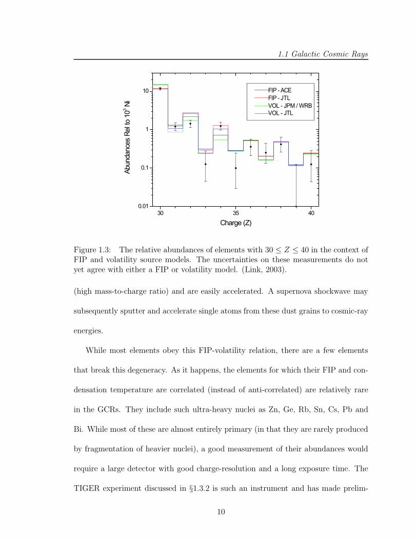
Figure 1.3: The relative abundances of elements with 30 ≤ Z ≤ 40 in the context ofFIP and volatility source models. The uncertainties on these measurements do notyet agree with either a FIP or volatility model. (Link, 2003).
(high mass-to-charge ratio) and are easily accelerated. A supernova shockwave may
subsequently sputter and accelerate single atoms from these dust grains to cosmic-ray
energies.
While most elements obey this FIP-volatility relation, there are a few elements
that break this degeneracy. As it happens, the elements for which their FIP and con-
densation temperature are correlated (instead of anti-correlated) are relatively rare
in the GCRs. They include such ultra-heavy nuclei as Zn, Ge, Rb, Sn, Cs, Pb and
Bi. While most of these are almost entirely primary (in that they are rarely produced
by fragmentation of heavier nuclei), a good measurement of their abundances would
require a large detector with good charge-resolution and a long exposure time. The
TIGER experiment discussed in §1.3.2 is such an instrument and has made prelim-
10
1.1 Galactic Cosmic Rays
inary measurements of the abundances of some of these nuclei. As can be seen in
Figure 1.3, TIGER has not yet provided definitive experimental evidence to support
either a FIP or a volatility model; further data from more balloon flights is needed.
1.1.3 Propagation and reacceleration
After being initially accelerated, the journey of a GCR through the interstellar medium
(ISM) can be quite complicated. During transport, GCRs encounter magnetic fields
of varying magnitudes and regions of differing densities that may change the state of
an energetic nucleus.
Spallation, or fragmentation, of a primary nucleus occurs mostly in interactions
with ambient hydrogen gas, for which the average density has been reported to be
0.34 ± 0.04 atoms/cm3 (Yanasak et al., 2001). In this way, a heavy parent nucleus
gives rise to a lighter nucleus with an energy less than or approximately equal to that
of the parent nucleus. An unstable daughter nucleus may decay to another species
if the half-life is less than the escape time from the Galaxy. Because of this, when
detected at Earth, GCRs are enhanced over solar system values in stable or long-lived
isotopes for which the production cross sections with hydrogen of abundant elements
such as C, N, O, Si, Mg and Fe are large enough to facilitate significant spallation.
It has long been known that the relatively rare elements in the solar system such
as Li, Be, B, Sc, Ti, and V are greatly enhanced due to their production by interac-
tions of C, N, O and Fe on ambient interstellar gas. The ratios of the abundances
of these secondary nuclei to their parent nuclei give a good indication of the amount
11

1.1 Galactic Cosmic Rays
of material traversed in the ISM. Specifically, comparison of observed abundances of
secondary radionuclides with galactic propagation models provide a good measure of
the residence time of GCRs in the Galaxy. Measurements of the long-lived radionu-
clides 10Be, 26Al, 36Cl and 54Mn agree well with an average galactic confinement time
of 15.0 ± 1.6 Myr before escape (Yanasak et al., 2001).
In particular, it is important to note the enhancement in the secondary radionu-
clides that decay only by electron capture, a feature attributed to the extreme energy-
dependence of the electron attachment cross section. Electron-capture-decay isotopes
propagating at several hundred MeV/nucleon are effectively stable in the GCRs,
whereas lower-energy electron-capture-decayisotopes have a much higher electron-
attachment cross section and will subsequently decay relatively quickly (see §4).
It has been argued that the distributed reacceleration of cosmic rays in the ISM
after their initial acceleration by a supernova shockwave plays a non-trivial role in
the propagation of GCRs. The invoking of some degree of reacceleration into a prop-
agation model has been shown to resolve discrepancies about the source abundances
of N, F, Na, Al, Cr and Mn. Silberberg et al. (1983) showed that incorporating
reacceleration into a simple propagation model alleviates the need to reduce the cal-
culated abundances of the electron-capture secondary isotopes 37Ar, 49V and 51Cr to
fit the data at 600 MeV/nucleon. Their results were somewhat inconclusive, however,
due to the simplicity of their model combined with the poor quality of isotopic data
available from previous experiments.
Osborne et al. (1988) have argued that since magnetohydrodynamic turbulence
12

1.2 Cosmic Rays in the heliosphere
is responsible for the spatial diffusion of GCRs in the ISM, it follows logically that
further scattering must also reaccelerate nuclei through the Fermi acceleration process
well after their initial acceleration at supernova shockfronts. Additionally, models
that incorporate some form of diffusive reacceleration have been shown to fit the
energy-dependent features of some secondary-to-primary abundance ratios such as
B/C (Letaw et al., 1993; de Nolfo et al., 2005). This thesis will address directly the
question of reacceleration with respect to electron-capture decay in GCRs, using
better data and a more sophisticated model of GCR propagation.
1.2 Cosmic Rays in the heliosphere
The journey through the heliosphere before being detected at or near Earth affects the
spectra of GCRs with energies below a few GeV/nucleon in a non-neglible way. This
section will give an overview of what is known about the solar cycle, the models that
can be used to parametrize the effects of solar modulation, and a brief description of
the model used in this study. It will later be demonstrated directly in this thesis that
over the course of the 22-year solar cycle, the amount of energy loss is greater during
periods of solar maximum than during periods of solar minimum.
1.2.1 The 22-year solar cycle
Galileo was most likely the first astronomer to study changes in the sun’s appearance
over time. During the summer of 1612, Galileo made detailed sketches of the surface
13

1.2 Cosmic Rays in the heliosphere
of the sun at approximately the same time every day, publishing his work in 1613 in
a work titled History and Demonstrations Concerning Sunspots and their Properties.
The first observation of some periodicity in the number of sunspots observed over
time is credited to Schwabe, who detailed sunspot activity for several years in the mid
1800s. From his observations, Schwabe identified that the number of sunspots went
from a minimum to a maximum over a period of 8 to 15 years (von Humboldt, 1850).
It has since been established that sunspot number increases during periods of high
solar activity, which is characterized by the switching of polarity of the sun’s magnetic
field.
The 22-year cycle can, in fact, be broken down into two ∼11-year cycles that
include two pairs of minimum and maximum activity. During the first stage of the
cycle, known as the A > 0 phase, the sun is relatively quiet; its magnetic field has
positive polarity at the solar north pole and negative polarity at the south pole. A
period of greater solar activity, known as solar maximum, follows as temperature
gradients and sunspot numbers increase on the surface of the sun. During this time,
the structure of the solar magnetic fields becomes more complex and solar wind
speeds increase. The next stage of minimum activity occurs at the A < 0 phase when
the magnetic field has reoriented itself, with positive polarity at the south pole and
negative polarity at the north. A similar period of maximum activity occurs as the
magnetic field returns to the A > 0 phase (Foukal, 1990).
14

1.2 Cosmic Rays in the heliosphere
1.2.2 Particle transport in the heliosphere
The magnetic fields produced in the dynamic solar cycle are carried out with the
supersonic solar winds stemming from the rotating sun. At any place in the inter-
planetary medium, the resultant field lines then describe, on average, an Archimedes
spiral with the sun at the origin.
Parker (1965) noted further that charged particles with gyroradii comparable in
size to that of magnetic irregularities in the outwardly flowing wind will be effectively
scattered by the fields. The scatter back and forth of energetic particles across mag-
netic lines of force cause them to random walk in the reference frame of the magnetic
irregularities. This large-scale random walk of charged particles in the heliosphere
can be reasonably approximated by a spherically-symmetric Fokker-Planck or diffu-
sion equation. The formalization of this work will be discussed in the next section.
Later work done by Jokipii et al. (1977) expanded on the Parker model identifying
the importance of gradient and curvature drifts on the solar modulation cosmic-ray
particles. Further work involved computer simulations that modeled a “wavy” neutral
magnetic current sheet extending from the solar equator created at the boundary
between field lines of opposite polarity protruding from the northern and southern
hemispheres of the sun. This work was furthermore able to explain the alternating
“flattening” effects in every other period of solar minimum as seen in neutron monitor
measurements (see Figure 1.4). During the A > 0 phase of the solar cycle, GCR nuclei
drift from the heliospheric polar regions toward their points of observation, whereas
15

1.2 Cosmic Rays in the heliosphere
Figure 1.4: The solid line shows the monthly-averaged, normalized count-rate ofcosmic-ray secondary neutrons as measured by the Climax Neutron Monitor from1951 to the present. The dotted line shows the monthly-average, normalized andsmoothed sunspot number over the same time period. Note the flattening out of thecosmic-ray flux during the two solar minimum periods in the 1970s and 1990s. Thesedata are provided courtesy of University of New Hampshire and National ScienceFoundation Grant ATM-9912341.
GCR nuclei drift inward along this wavy magnetic current toward Earth during the
A < 0 phase. As the A > 0 phase sets up, GCRs diffuse more easily toward Earth
and maintain their intensity for a longer period of time. Particles observed during
the A < 0 phase will have diffused along the wavy current sheet, gaining in intensity
as the sheet smooths out at the peak of solar minimum, and losing intensity as they
diffuse for longer and longer periods of time as the waviness intensifies toward the
next period of solar maximum. In addition to drifts along the current sheet, the
spiral nature of the solar magnetic fields at 1 AU invokes tangential drift effects as
16

1.2 Cosmic Rays in the heliosphere
well. The effect of these drifts during the A > 0 phase is a net flow of positively-
charged particles along the field lines in the opposite direction to solar rotation, and
a net flow of negatively-charged particles (electrons) in the direction of solar rotation
(Jokipii and Thomas, 1981).
1.2.3 Diffusion, convection and adiabatic energy loss
It has long been known that the GCRs suffer a decrease in flux as they diffuse in
the magnetic irregularities expanding outward with the solar wind, and that this
decrease in flux is more severe during periods of high solar activity. One of the most
important breakthroughs of the Parker theory was developed further in a later work
(1966). Parker noted that while the primary effect of the solar wind is to convect
cosmic rays out of the solar system, the random walk of the charged cosmic-ray nuclei
in the expanding magnetic field continually serves to decelerate them adiabatically.
Rygg and Earl (1967) provided the first experimental evidence for this claim by noting
that this theory explained the observed roll over in the cosmic-ray proton spectrum
below ∼ 250 MeV/nucleon where the differential intensity is simply proportional to
energy. Further work by von Rosenvinge and Paizis (1981) demonstrated that cosmic-
ray species with different spectral shapes were modulated differently and suffered
differing amounts of energy loss.
Parker’s spherically-symmetric equation was elucidated by Goldstein et al. (1970).
17

1.2 Cosmic Rays in the heliosphere
The equation,
1
r2
∂
∂r
(
r2V U)
− 1
3
[
1
r2
∂
∂r
(
r2V)
] [
∂
∂T(αTU)
]
=1
r2
∂
∂r
(
r2κ∂U
∂r
)
, (1.1)
allows for the effects of convection, diffusion and energy loss where κ(r, T ) is the
radial diffusion coefficient, V (r) is the solar wind speed, α(T ) = T+2M0
T+M0for a particle
of rest energy M0, and U(r, T ) is the cosmic-ray number density per unit kinetic
energy interval.
Gleeson and Axford (1968) simplified this model, separating the diffusion coef-
ficient into radial- and rigidity-dependent components, and related the intensity of
cosmic rays inside the heliosphere to their interstellar intensity by way of a single
energy-loss parameter. This model is now known as the “forcefield” approximation
with the single parameter, φ, thought of as the potential difference through which a
charged particle must move from infinity to its point of detection at earth. This φ
has a single value for all species and is related to Φ, the amount of energy per nucleon
that a particle will lose coming in from infinity. The value of φ is therefore higher
during periods of solar maximum than during periods of solar minimum.
1.2.4 This solar modulation model
While this simplified forcefield approximation works well for nuclei with energies
above several hundred MeV/nucleon, it begins to break down at lower energies. A
rigorous numerical solution of the Fokker-Planck equation has been shown to agree
better with the data when approximating the spectra of lower-energy GCRs at earth,
18

1.3 Detection
as in (Fisk, 1971; Fisk et al., 1971).
For the purposes of this study, the effects of solar modulation have been approxi-
mated as an 11-year cycle using only this spherically-symmetric model, ignoring the
different drift effects from the A > 0 to the A < 0 phase of the solar cycle. We pa-
rameterize the amount of solar modulation present over the course of the solar cycle
using a φ parameter similar to that used in the forcefield approximation. Following
the formalism of Goldstein et al. (1970) and the results of Davis et al.(2001) and
George et al. (2005), the diffusion coefficient, κ, is a function of distance to sun, r,
constant solar wind velocity equal to 400 km/s, the rigidity, R, and velocity β of the
GCR in question, and is related to the modulation parameter, φ, by
κ(r, R, β, φ) ∝
β
φ(if R < 160 MV)
β√
R
φ(if 160 < R < 750 MV)
βR
φ(if R > 750 MV)
(1.2)
1.3 Detection
While techniques of detection for high-energy nuclei have varied somewhat in the last
century, the basic principles have remained. A charged nucleus entering a medium has
a certain probability of interacting either by losing energy to ionization in inelastic
collisions with the atoms in the material, or by strongly interacting with another
nucleus in the material, thereby creating other particles (mesons and photons) whose
charged decay products (muons, electrons, and positrons) may interact via ionization
energy loss. The amount of energy that a charged particle deposits per unit pathlength
19
1.3 Detection
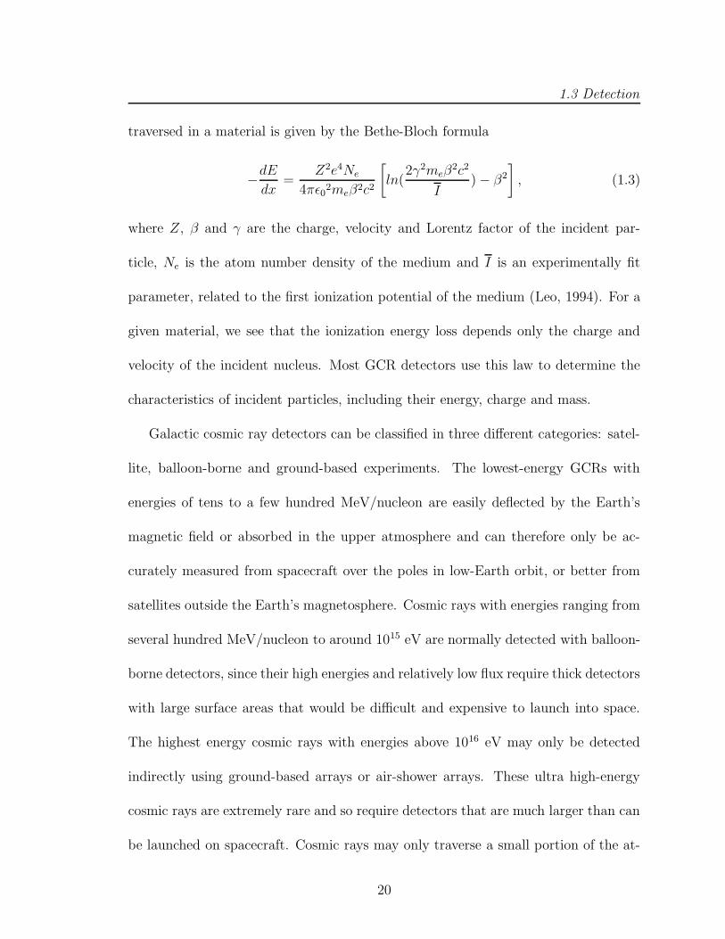
traversed in a material is given by the Bethe-Bloch formula
−dEdx
=Z2e4Ne
4πε02meβ2c2
[
ln(2γ2meβ
2c2
I) − β2
]
, (1.3)
where Z, β and γ are the charge, velocity and Lorentz factor of the incident par-
ticle, Ne is the atom number density of the medium and I is an experimentally fit
parameter, related to the first ionization potential of the medium (Leo, 1994). For a
given material, we see that the ionization energy loss depends only the charge and
velocity of the incident nucleus. Most GCR detectors use this law to determine the
characteristics of incident particles, including their energy, charge and mass.
Galactic cosmic ray detectors can be classified in three different categories: satel-
lite, balloon-borne and ground-based experiments. The lowest-energy GCRs with
energies of tens to a few hundred MeV/nucleon are easily deflected by the Earth’s
magnetic field or absorbed in the upper atmosphere and can therefore only be ac-
curately measured from spacecraft over the poles in low-Earth orbit, or better from
satellites outside the Earth’s magnetosphere. Cosmic rays with energies ranging from
several hundred MeV/nucleon to around 1015 eV are normally detected with balloon-
borne detectors, since their high energies and relatively low flux require thick detectors
with large surface areas that would be difficult and expensive to launch into space.
The highest energy cosmic rays with energies above 1016 eV may only be detected
indirectly using ground-based arrays or air-shower arrays. These ultra high-energy
cosmic rays are extremely rare and so require detectors that are much larger than can
be launched on spacecraft. Cosmic rays may only traverse a small portion of the at-
20

1.3 Detection
mosphere before strongly interacting; at high energies, interacting GCRs precipitate
enormous electromagnetic “showers.” Charged particles in these showers may fluo-
resce or emit Cherenkov radiation over a large volume in the atmosphere, permitting
the use of ground-based imaging detectors or large areas of ground-based Cherenkov
counters spread over many square kilometers.
1.3.1 Advanced Composition Explorer
The Advanced Composition Explorer (ACE ) mission was designed to measure so-
lar wind speeds and magnetic fields, in addition to the composition of solar en-
ergetic particle events (SEPs), ACRs and GCRs (Stone et al., 1998c). The ACE
spacecraft was launched on August 25, 1997 and placed into a halo orbit about
the L1 Lagrange point, 0.01 AU sunward from earth. Of the nine instruments
on ACE, the Cosmic Ray Isotope Spectrometer (CRIS) instrument, discussed fur-
ther in §2, is the highest energy instrument and measures the abundances of cos-
mic ray isotopes. A more complete description of the instrument can be found in
Stone (1998a). The Solar Isotope Spectrometer (SIS) measures the isotopic com-
position of particles with ∼ 10 to ∼ 100 MeV/nucleon, which include SEPs, ACRs
and GCRs (Stone et al., 1998b). At lower energies, the Ultra Low Energy Isotope
Spectrometer (ULEIS) measures SEP and ACR elemental abundances from ∼ 45
keV/nucleon to a few MeV/nucleon (Mason et al., 1998). The Solar Energetic Par-
ticle Ionic Charge Analyzer (SEPICA) measures charge states for ions from ∼ 200
keV/nucleon to ∼ 5 MeV/nucleon (Mobius et al., 1998). The Electron, Proton, and
21
1.3 Detection
Alpha Monitor (EPAM) measures electrons and ions from 40 to 50 keV and ele-
mental abundances of ions with ∼ 500 keV/nucleon (Gold et al., 1998). The Solar
Wind Ion Composition Spectrometer (SWICS), the Solar Wind Ion Mass Spectrom-
eter (SWIMS) and the Solar Wind Electron, Proton and Alpha Monitor (SWEPAM)
measure the chemical and isotopic composition of solar wind ions with speeds above
∼ 300 km/s (Gloeckler et al., 1998). The MAG instrument measures the local in-
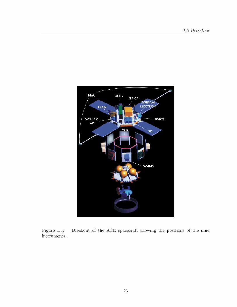
terplanetary magnetic fields (Smith et al., 1998). Figure 1.5 shows a breakout of the
ACE spacecraft.
1.3.2 Trans-Iron Galactic Element Recorder
Like many other balloon-borne GCR detectors, the Trans-Iron Galactic Element
Recorder (TIGER) instrument was designed to probe rare cosmic rays, while ad-
hering to a much smaller budget than their satellite counterparts. The detector was
created in order to measure the elemental abundances of ultra-heavy galactic cos-
mic rays (UHGCRs) with 30 ≤ Z ≤ 40 in the energy range ∼ 800 MeV/nucleon
to a few GeV/nucleon. It served as an engineering model of the large Heavy Nuclei
Experiment (HNX ) designed for space flight. As discussed further in §1.1.2, better
measurements of elements in this charge range may begin to resolve the problem of
whether cosmic rays are preferentially accelerated according to a low-FIP model or a
refractory model.
The TIGER instrument was flown once from Lynn Lake, Manitoba in Canada in
August 1995 and once from Fort Sumner, New Mexico in September 1997. Although
22
1.3 Detection
Figure 1.5: Breakout of the ACE spacecraft showing the positions of the nineinstruments.
23
1.3 Detection
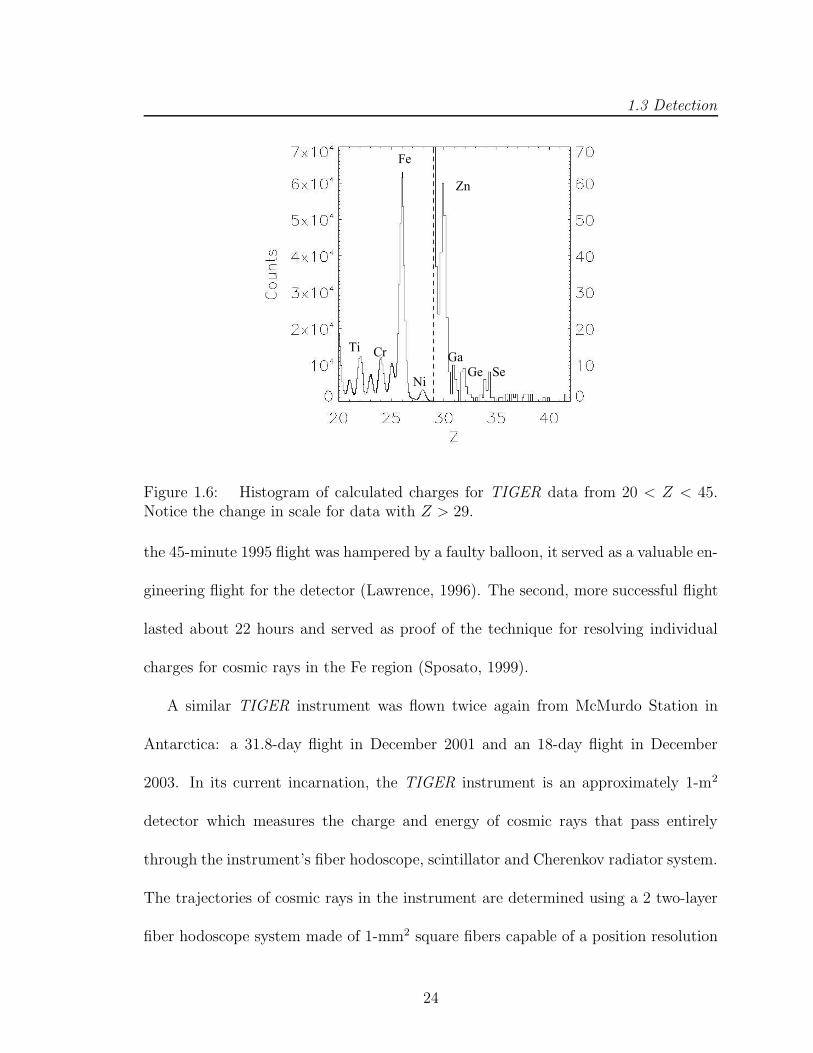
Figure 1.6: Histogram of calculated charges for TIGER data from 20 < Z < 45.Notice the change in scale for data with Z > 29.
the 45-minute 1995 flight was hampered by a faulty balloon, it served as a valuable en-
gineering flight for the detector (Lawrence, 1996). The second, more successful flight
lasted about 22 hours and served as proof of the technique for resolving individual
charges for cosmic rays in the Fe region (Sposato, 1999).
A similar TIGER instrument was flown twice again from McMurdo Station in
Antarctica: a 31.8-day flight in December 2001 and an 18-day flight in December
2003. In its current incarnation, the TIGER instrument is an approximately 1-m2
detector which measures the charge and energy of cosmic rays that pass entirely
through the instrument’s fiber hodoscope, scintillator and Cherenkov radiator system.
The trajectories of cosmic rays in the instrument are determined using a 2 two-layer
fiber hodoscope system made of 1-mm2 square fibers capable of a position resolution
24

1.3 Detection
of about 1.7 mm. Charge and energy assignments for particles with energies less than
∼ 2.5 GeV/nucleon are achieved using an acrylic Cherenkov radiator, located in the
middle of the detector, and four polyvinyl toluene scintillators, located on the top
and bottom of each two-plane hodoscope unit. The charges and energies of particles
above ∼ 2.5 GeV/nucleon are determined using the acrylic and aerogel Cherenkov
radiators, also located in the middle of the detector. Details on the design, electronics
and response of these detectors can be found in Link (2003).
The 2001 flight provided good data for ∼ 100 events in the 30 ≤ Z ≤ 40 range
(see Figure 1.6). While such low statistics prohibit conclusive evidence of either a
FIP or volatility source for GCRs, further evidence may come from the analysis of
data from the 2003 TIGER flight and from future flights of the TIGER instrument,
such as one tentatively scheduled for 2007.
1.3.3 Other Galactic cosmic ray detectors
Spacecraft Experiments
The CRIS experiment on the ACE spacecraft is one of the most recent in a long line
of cosmic ray detectors. Both Voyager spacecraft, which launched in 1977, carried on-
board High Energy Telescope (HET) experiments which were designed to measure el-
emental abundances of cosmic rays from H to Fe and beyond in the energy range from
1 - 500 MeV/nucleon, with the possibility of resolving individual isotopes for GCRs
lighter than 16S in the energy range from 2 - 75 MeV/nucleon (Stone et al., 1977).
25

1.3 Detection
More recent studies have been able to further resolve the isotopes from 20Ca to 26Fe
in the energy range from 100 - 300 MeV/nucleon, with resolutions from 0.40 amu to
0.60 amu (Lukasiak et al., 1997).
The International Sun-Earth Explorer 3 (ISEE-3 ) spacecraft was launched in late
1978, and had onboard two instruments capable of resolving GCRs elements and iso-
topes (Wiedenbeck, 1992). Using data from these instruments, Leske (1993) reported
measurements of isotopes as heavy as 28Ni at an energy of ∼ 325 MeV/nucleon.
The first in a series of Interplanetary Monitoring Platform (IMP) spacecraft was
launched in 1963 and made many early measurements of magnetic fields, plasmas, and
energetic particles, including cosmic rays. The IMP-7 and -8 spacecraft, launched
in 1972 and 1973, respectively, made some of the best GCR measurements which
included elemental spectra for C, O, Ne, Mg and Si (Garcia-Munoz et al., 1977).
Building on this work, the C2 instrument on the High Energy Astronomy Obser-
vatory 3 (HEAO-3 ), which was active from 1979 to 1981, made detailed elemental
abundance measurements from 4 ≤ Z ≤ 28 in the range from 620 MeV/nucleon to
35 GeV/nucleon (Engelmann et al., 1990).
The Cosmic Ray Nuclei experiment (CRN ) was launched on the Space Shuttle in
1985. Using gas Cherenkov counters and transition radiation detectors, CRN made
significant measurements of elemental B, C, N, O and up to the Fe group at energies
of about 2 TeV/nucleon (Swordy et al., 1990; Swordy et al., 1993).
The Ulysses spacecraft was launched aboard the Space Shuttle Discovery in 1990
into a highly eccentric orbit at nearly 90 to the ecliptic, for the purpose of doing
26

1.3 Detection
fast pole-to-pole scans of the Sun. DuVernois and Thayer (1996) have also reported
elemental abundances of GCRs from 4 ≤ Z ≤ 28 at ∼ 185 MeV/nucleon as measured
by the HET instrument onboard Ulysses.
Balloon-borne experiments
Since satellite experiments are often quite expensive and limited to smaller and
lighter detectors, balloon-borne experiments can be reliable alternatives that can
often achieve the same or similar scientific goals at a fraction of the cost. While the
exposure time for balloon experiments is limited to a few tens of days, balloon-borne
GCR detectors can be larger and heavier, with much greater geometry factors than
can be achieved in space. In addition, even at the highest altitudes, scientific balloon
payloads still remain underneath a few g/cm2 of air and close enough to earth that
they are subject to certain levels of geomagnetic cutoff that decrease the local flux
of charged cosmic rays. Due to this fact, the most ideal locations for balloon-borne
cosmic-ray detectors are at high latitudes, near the north and south poles, where
there is no geomagnetic cutoff and balloons can remain aloft for several weeks with-
out invading commercial airline space or floating above populated areas. In the end,
while also securing good scientific data, balloon experiments can also serve as test
prototypes for future satellite experiments.
A balloon-borne GCR detector headed by the Marshall Space Flight Center in
Huntsville, Alabama was launched from Sioux Falls, South Dakota in 1976 for a total
flight time of 17 hours at an atmospheric depth of about 5 g/cm2. This detector,
27

1.3 Detection
which was capable of measuring GCRs with energies from 500 MeV/nucleon to 2
GeV/nucleon, made good measurements of the elemental spectra of B, C, N, O, Ne,
Mg, Si and Fe (Derrickson et al., 1992).
A balloon-borne detector developed by a group at the University of New Hamp-
shire was flown twice from Churchill, Manitoba in Canada, once from Sioux Falls,
South Dakota in 1974 and once again in 1976 from Sioux Falls, South Dakota un-
derneath an average atmosphere of ∼ 3 g/cm2 for a total of about 65 hours. This
scintillation and Cherenkov detector measured the charge composition of GCRs be-
tween 3 ≤ Z ≤ 28 from ∼ 0.3 to ∼ 50 GeV/nucleon (Lezniak and Webber, 1978).
The University of Minnesota’s Cosmic Ray Isotope Instrument System (CRISIS ),
a nuclear emulsion detector, was launched from Aberdeen, South Dakota in May 1977
underneath ∼ 2.6 g/cm2 of atmosphere and was able to sample GCRs at energies
ranging from 430-560 MeV/nucleon and 650-900 MeV/nucleon during a period of
extreme solar quiet time. This 57-hour flight resulted in measurements of isotopic
spectra from Si to Ni during a period of low solar modulation (Young et al., 1981).
More recently, Long Duration Ballon flights from McMurdo Station, Antarctica
have ushered in a new era of scientific ballooning, enabling detectors to fly for periods
of several weeks in a region of low geomagnetic cutoff. The Balloon-borne Experiment
with a Superconducting Spectrometer (BESS ) has completed several flights, includ-
ing one from Antarctica, to measure the abundance of anti-protons and possible anti-
Helium in the cosmic rays (Yoshida et al., 2004). Detectors such as the Transition
Radiation Array for Cosmic Energetic Radiation (TRACER) (Gahbauer et al., 2004)
28

1.3 Detection
and the Cosmic Ray Energetics and Mass (CREAM ) instrument (Seo et al., 2004)
have begun to measure elemental abundances of GCRs with energies up to ∼ 1015 eV.
In time, a better understanding of composition at this “knee” in the cosmic ray spec-
trum should start to shed light on the question of how cosmic rays above ∼ 1015 eV
are accelerated.
Ground-based experiments
In order to detect ultra-high energy cosmic rays (UHECRs), those with energies
in excess of around 1017 eV, the size of the active area of the detector becomes
increasingly important, as is well demonstrated in Figure 1.2. Cosmic rays with
these energies are so rare that to get reasonable statistics, one must design a detector
with an extremely large active area. Additionally, since cosmic-ray nuclei will interact
very high in the atmosphere, they can only be detected indirectly, either by measuring
the shower of secondary charged particles reaching the ground or by measuring the
light emitted by interactions of the secondary muons, electrons and positrons with
molecules in the atmosphere. The Akeno Giant Air Shower Array AGASA and the
Fly’s Eye experiments are two such detectors that have been in operation since the
early 1990s. The AGASA detector covers an area of about 100 km2 and detects
the cosmic-ray-induced showers of charged secondary particles using a large network
of surface plastic scintillators, underground muon detectors and water Cherenkov
detectors. The Fly’s Eye detector (modified more recently and known as HiRes Fly’s
Eye) uses two telescopes to detect secondary charged particles by fluorescence from
29
1.3 Detection
nitrogen molecules in the atmosphere. One of the most exciting recent controversies
in cosmic ray astrophysics involves the discrepancy between the results from these
two experiments.
As discussed briefly at the beginning of this chapter, in the center of momentum
frame, an interaction between a ∼ 1020 eV cosmic ray and the ∼ 10−3 eV cosmic
microwave background leaves enough energy for the creation of a pion which consid-
erably saps the initial energy of the UHECR. With a corresponding mean pathlength
of only 50 to 100 Mpc in the ISM, provided there are no local sources of UHECRs,
one should not expect to detect any cosmic rays above the energy threshold.
Galactic cosmic rays are also widely known to be almost entirely isotropic (having
no preferred arrival direction) due to scattering from galactic magnetic fields. It is
presumed however, that UHECRs may exhibit some anisotropy since they should be
scattered relatively little by these magnetic fields.
As it stands, the AGASA collaboration have presented findings that indicate a
violation of the GZK cutoff (Takeda et al., 1998) whereas the HiRes collaboration
observes the predicted end of the spectrum under 1020 eV (Abbasi et al., 2004b).
The AGASA and HiRes collaborations disagree further in their study of anisotropies
(Takeda et al., 1999; Abbasi et al., 2004a).
The AUGER project, named after Pierre Auger, the discoverer of extensive air
showers, has only recently begun to come online. Located in the Mendoza province in
Argentina and with an active area of ∼ 3000 km2, AUGER is to be the world’s largest
cosmic ray detector. With a combination of water Cherenkov tanks and fluorescence
30
1.4 Scope of this work
detectors, it is hoped that the AUGER project will put an end to the controversy
surrounding UHECRs (Etchegoyen, 2004).
1.4 Scope of this work
The energy dependence of electron-capture decay in GCRs can provide us with valu-
able information about the processes that govern energy loss and energy gain during
the propagation of a GCR from the source to the detector. Secondary radionuclides
whose sole decay process is by electron-capture exhibit distinct features in their spec-
tra, owing to the highly energy-dependent cross section for electron attachment, and
subsequently short decay half-lives. This dissertation exhibits work with new mea-
surements of the rare isotopes involved in electron-capture decay in the sub-Fe regime,
taking advantage of both the large geometry factor and excellent isotopic resolution of
the CRIS detector. The spectral features in the daughter-to parent abundance ratios
for sub-Fe isotopes involved in electron-capture decay provide new direct evidence
for energy-loss in the due to solar modulation in the heliosphere. In addition, com-
parison of the energy dependence of these electron-capture-decay abundance ratios
during solar minimum to galactic propagation models that incorporate some amount
of diffusive reacceleration in the ISM serves to demonstrate that GCRs experience
little or no reacceleration during propagation in the Galaxy.
31

Chapter 2
Cosmic Ray Isotope Spectrometer
Figure 2.1: The Cosmic Ray Isotope Spectrometer. Visible are the image-intensifiedCCD cameras, the high-voltage power supplies and the SOFT hodoscope (large squarearea). See Figure 2.2 for more detail.
The Cosmic Ray Isotope Spectrometer (CRIS) onboard the NASA Advanced Com-
position Explorer (ACE ) came online three days after launch of the spacecraft on Au-
gust 25, 1997. As a detector, CRIS is one of the largest and best of its kind, measuring
the charge, mass and energy of cosmic rays with 2 ≤ Z ≤ 30 with exquisite mass
32
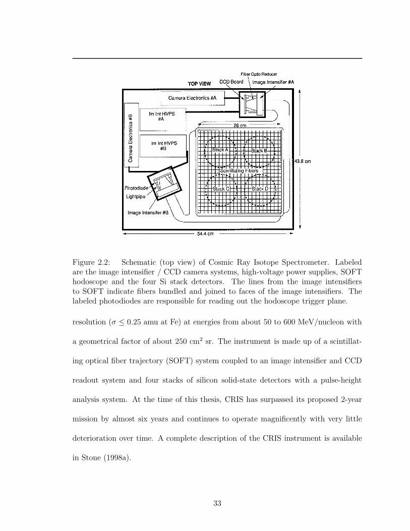
Figure 2.2: Schematic (top view) of Cosmic Ray Isotope Spectrometer. Labeledare the image intensifier / CCD camera systems, high-voltage power supplies, SOFThodoscope and the four Si stack detectors. The lines from the image intensifiersto SOFT indicate fibers bundled and joined to faces of the image intensifiers. Thelabeled photodiodes are responsible for reading out the hodoscope trigger plane.
resolution (σ ≤ 0.25 amu at Fe) at energies from about 50 to 600 MeV/nucleon with
a geometrical factor of about 250 cm2 sr. The instrument is made up of a scintillat-
ing optical fiber trajectory (SOFT) system coupled to an image intensifier and CCD
readout system and four stacks of silicon solid-state detectors with a pulse-height
analysis system. At the time of this thesis, CRIS has surpassed its proposed 2-year
mission by almost six years and continues to operate magnificently with very little
deterioration over time. A complete description of the CRIS instrument is available
in Stone (1998a).
33

2.1 Scintillating Optical Fiber Trajectory system
Figure 2.3: Schematic (side view) of SOFT and Si stack detector system. The triggerplane is a set of two x and y layers. The three sets of planes below the trigger formthe hodoscope. The silicon wafers forming each of the four telescopes are labeled E1through E9. Detectors E3 through E8 are each made of two 3-mm wafers whereasE1, E2 and E9 are single wafers. The numbers to the right are vertical distances incm from a reference plane.
2.1 Scintillating Optical Fiber Trajectory system
The Scintillating Optical Fiber Trajectory (SOFT) system is the six-layer fiber ho-
doscope system that was created at Washington University in St. Louis, made up of
almost 10,000 polystyrene fibers doped with scintillation dyes. The fibers are 180 µm
square of scintillator with 10 µm of acrylic cladding on each side. The cladding is
coated in a black ink to prevent any optical coupling between adjacent fibers. The
fibers are laid parallel to one another to form a plane, and are coupled at each end
34

2.2 Silicon stack detector system
to an image intensifier. The active area of each fiber layer is 26 cm × 26 cm. The
fibers from each plane are bonded together in a 3 mm × 24 mm rectangular output
before being coupled to the face of the image intensifier. The intensified image is then
read out by a 244 × 550 pixel charge-coupled device (CCD). Only one image inten-
sifier/CCD system is required to properly read out the fibers; the other is redundant
in case of failure, but has not been needed throughout the almost eight years to date.
2.2 Silicon stack detector system
There are four silicon detector telescopes each composed of 15 silicon disks that are
∼ 3 mm thick. The wafers are 10 cm in diameter and made of almost entirely pure
silicon, by means of the lithum compensation technique (Allbritton et al., 1996). The
wafers are designed two different ways, single-grooved with a 68 cm2 active area and
double-grooved, with a 57 cm2 active area. Each stack contains 4 single-grooved
wafers and 11 double-grooved wafers. The 15 wafers are mounted to a common frame
for all four stacks using the outermost groove; the double-grooved design serves to
identify and reject particles which enter or exit in the guard rings (the area between
the grooves). The detectors are labeled E1 through E9, where E1, E2 and E9 are
single Si wafers and E3 through E8 are each composed of a pair of wafers. Detectors
E1, E8 and E9 are single-grooved detectors and E2 through E7 are double-grooved
(see Figure 2.3). Good events for this study are limited to those that come to rest in
detectors E2 through E8 without penetrating the guard rings or the E9 detector.
35

2.3 CRIS inflight data output
It was found during preflight testing that each wafer contained a small “dead
layer” amounting to approximately 55-70 µm in each wafer, due most likely to heavily
lithiated regions in the silicon. There are also larger layers in which an incomplete
collection of electrons obscures the results. The cuts and corrections made for these
dead-layer effects are discussed further in §3.1.5.
There are 32 pulse-height analyzers (PHAs) in CRIS which read out the entire
system of silicon detectors. The four E1 detectors are read out in four separate PHAs
whereas detectors E2 through E9 are summed in two pairs of telescopes, and each
two-telescope detector pair is read by one PHA. The six guard rings in each telescope
are paired and read out in a similar way.
2.3 CRIS inflight data output
2.3.1 Event data
A good event for CRIS must create both a signal in the SOFT trigger plane and in
at least detectors E1 and E2, and no signal in any of the guard rings. For each event,
an onboard microprocessor reads a 12-bit signal from all PHAs with signals above
their nominal thresholds, video data from the SOFT system, which consist of the
position and intensity of every above-threshold pixel in the CCD. The two bright-
est SOFT centroids (regions of several bright adjacent pixels) are then determined
onboard. These events, which may differ in length from 31 bytes to 162 bytes, are
then compressed to maximize output for the small bitrate (58 bytes/sec) allowed for
36

2.4 The dEdx
· E technique
transmitting data from the instrument.
2.3.2 Housekeeping and rate data
In addition to voltages, currents and temperature readings, trigger rates for each
trigger plane and the coincidence of the trigger planes are recorded. Three different
livetime rates are calculated for Z = 1, Z = 2 and Z > 2 and included in the
datastream. In the end, all event, housekeeping and rate data are multiplexed over a
256-second instrument cycle and telemetered down to earth.
2.4 The dEdx
·E technique
If a particle with charge Z, mass number A, and initial kinetic energy E penetrates
matter of thickness L, it will emerge with a kinetic energy E ′ such that
R
(
Z,A,E
A
)
− R
(
Z,A,E ′
A
)
= L, (2.1)
where R is its range in the given material as a function of energy. In general, for a
detector of thickness L0, the thickness traversed, L, is given by
L = L0 sec(θ). (2.2)
where θ is the angle of the particle trajectory with respect to the normal to the
detector. As discussed further in Stone (1998a) and in Appendix B, the range of a
nucleus in silicon can be expressed
R
(
Z,A,E
A
)
≈ kA
Z2
(
E
A
)α
, (2.3)
37

2.4 The dEdx
· E technique
Figure 2.4: The evolution of the data from pulse height values to calculated chargefor data with Z ≥ 20 that come to rest in telescope 0, detector E3. (a) sum of pulseheights in detectors E1 and E2 versus the pulse height in E3. (b) sum of pulse heightsin detectors E1 and E2 corrected for cos(θ) versus the pulse height in E3. Plots (a)and (b) demonstrate the need for a hodoscope to correct for the incident angle of theparticle in ∆E.
where α ≈ 1.7 (see Table B.1. Note that in Appendix B, E is defined as energy per
nucleon, i.e. E ≡ EA). Combining Equations 2.1 and 2.3, it can be shown that
A ≈[
k
Z2L
]1
α−1
(Eα − E ′α)1
α−1 . (2.4)
Since AZ
= 2 + ε where ε ≤ 0.4, for all the isotopes with a half-life long enough to be
found in the GCRs, the charge of the nucleus can be found
Z ≈[
k
L(2 + ε)α−1
]1
α+1
(Eα − E ′α)1
α+1 . (2.5)
In practice, if one determines first the integer value of Z by Equation 2.5 for any ε
such that 0 ≤ ε ≤ 0.4, the element peaks are so well-separated that determining the
isotope mass follows easily from Equation 2.4. In this way, both Z and A can be
calculated from E, E ′, a penetrated thickness L0 and an angle of incidence θ.
38

2.4 The dEdx
· E technique
Thinking about it another way, let ∆E be the energy deposited in detectors of
total thickness L that the particle penetrates entirely. From the Bethe-Bloch formula,
∆E
L≈ dE
dx= Z2 · f(β), (2.6)
where f(β) is a function of the nucleus’ velocity. The total energy of the nucleus can
then be written
E = A · g(β), (2.7)
where g(β) is another function of the particle’s velocity. The combination of these
two equations gives
∆E
L·E ≈ Z2A · f(β) · g(β). (2.8)
Since no two isotopes have the same Z2A, when ∆EL
is plotted versus E, discrete charge
bands will form, as is shown in Figure 2.4. When applying an additional correction
to L0 for depth variations in the silicon stack detectors, clear isotope bands will form
within each charge band. The data presented in Figure 2.4 have not been corrected
for these depth variations.
39

Chapter 3
Data Analysis
Since the CRIS instrument came online on August 28, 1997, it has been sending
back superb data on galactic cosmic rays in the energy range from about 50 to 600
MeV/nucleon. Although CRIS is equipped to resolve isotopic abundances for elements
from 2 ≤ Z ≤ 28, inefficiencies in the Scintillating Optical Fiber Trajectory (SOFT)
system at low-Z make measuring He, Li and Be difficult. In this dissertation, I will
only be concerned with isotopic abundances of elements with 5 ≤ Z ≤ 28.
In order to properly analyze CRIS data, it is necessary to determine the charge
and mass of each incident nucleus from the pulse heights measured in the Si detectors,
while correcting for the amount of material traversed in the detector from the angle
measured in the hodoscope. Abundances of each isotope are found by fitting the
mass histograms for each detector (see Appendix A). Making comparisons between
isotopes requires making adjustments for both range-energy and spectral shape (see
Appendix B).
40

3.1 Selecting usable data with xpick
3.1 Selecting usable data with xpick
Certain cuts and exclusions are necessary to ensure that usable data are not contam-
inated with particles that interact in the detector, come to rest in the Si dead layers,
or pass too close to the guard rings. Furthermore, since periods of high solar activity
also compromise the integrity of the CRIS data acquisition system, data collected
during these times must also be rejected. The xpick routines (version 1.1) developed
at Caltech provide first-order cuts and corrections to the data. Any higher-order cuts,
corrections or adjustments have been implemented in code that I have written.
3.1.1 Preliminary exclusion criteria
Events that are eliminated include those that occur less than 130 ms after another
event, those that trigger an event in more than one of the four telescopes, and those
that penetrate entirely through the Si stack. In addition, particles are rejected whose
straight-line trajectory fits deviate by more than 5 σ from the line defined by the
three xy hodoscope pairs in the SOFT system, based on a set of predetermined,
empirically-derived trajectory fits. Furthermore, xpick ensures that events that pass
within 500 µm of the edge of the SOFT hodoscope active area or within 500 µm of
the guard ring in all detectors (E1 through E8) are excluded. Finally, only events
that come to rest in detectors E2 through E8 are included in the analysis.
41

3.1 Selecting usable data with xpick
3.1.2 Charge consistency
The xpick program also tests the charge consistency for each event that stops in one
of detectors E3 through E8 by three different methods, in order to verify that the
values of Z are consistent with one another. Using the dEdx
·E technique described in
§2.4, Zest is defined such that dE is the sum of the energy deposited in all detectors
above the stopping detector and E ′ as the energy deposited in the stopping detector,
Zest E1 is defined using dE as the energy deposited in the first detector only while E ′
is the sum of the energy deposited in all subsequent detectors including the stopping
detector, and Zest LAST defines dE as the energy deposited only in the detector
above the one in which the particle stopped, with E ′ as the energy deposited in
the stopping detector only. Subsequently, two ratios are extablished: Z ratio E1 is
Zest E1 divided by Zest and Z ratio LAST is Zest LAST divided by Zest. Events
are only included that have Z ratio E1 and Z ratio LAST that deviate by less than
5σ from the mean of an empirically derived distribution based on Zest for all detectors
and telescopes. This process enables xpick to exclude events that arise from heavier
nuclei that may have fragmented inside the CRIS instrument. It has been shown
that the cuts described in this section and in §3.1.1 eliminate fully 2/3 of the initial
number of events for isotopes in the Fe group (Niebur, 2001).
42
3.1 Selecting usable data with xpick
3.1.3 Mass calculation
The mass estimates (in amu) for each event are calculated a number of ways, de-
pending on the detector in which a particles comes to rest. For a nucleus stopping in
detector i, there are i − 1 different masses calculated, such that a particle stopping
in detector E8 will have values for mass1 through mass7. The ith mass is obtained
using the ith detector as dE and the sum of the energy deposited in all subsequent
detectors, including the stopping detector, as E ′; the value is then computed using
Equation 2.4 where E ≡ dE +E ′ and L = L0 secθ is adjusted for depth variations in
the silicon stack detectors. For example, for a particle stopping in detector E8, mass5
is calculated using E5 as dE and the sum of the energy deposited in E6, E7 and E8
as E ′; L0 is adjusted according to thickness maps at the x-y point of entry into each
silicon wafer. Then mass avg is calculated as the weighted average of mass1 through
mass7. Each mass value is weighted by 1σM i
2 where σM is the empirically derived
mass resolution (amu) for each of mass1 through mass7.
3.1.4 Depth calculation
Once the charge and mass of an incident nucleus have been calculated, it is left to
determine the depth in µm at which the particle came to rest in the stopping detector,
when projected on the vertical axis. This value, known as rp proj is calculated in
the following way. The integral value of the charge of the incident nucleus, called iZ,
is determined from the method described in §3.1.2. An approximation of the mass,
43

3.1 Selecting usable data with xpick
called Mest, is then derived using the sum of energy deposited in all penetrated
detectors above the stopping detector as dE and the stop detector as E ′. The range
in g/cm2 is then derived using a range-energy routine for nuclei in silicon based on
Andersen and Ziegler (1977). The value of rp proj is then defined as this range in
µm multiplied by cosθ to find the projected depth, where θ is the incident angle of
the nucleus on the detector.
3.1.5 Geometrical cuts and mass avg corrections
In addition to the cuts and adjustments that are applied in xpick, other criteria have
been imposed in order to improve the quality of the data. As well as requiring that
a particle not pass too close the guard ring in a certain detector, it is important to
exclude particles that may have come to rest in or near a Si dead layer. There are two
features, which can be readily seen in Figure 3.1, that require special attention. Two
of the parameters that xpick determines for each event are rp proj, which gives the
depth in microns at which the particle comes to rest in a given detector (see §3.1.4),
and mass avg (see §3.1.3). The upward turn in mass at small rp proj is most likely
caused by a breakdown of the range-energy relation, whereas the case of mass avg
being double-valued at high rp proj is caused by particles that come to rest in a
dead layer in the E ′ detector or next detectors. When this occurs, the resulting pulse
height readout will be less than the actual amount of energy remaining when the
particle entered the E ′ detector and the particle will seem to have a smaller mass.
In order to remove data in the dead layer region, a cut was made excluding all
44

3.1 Selecting usable data with xpick
Figure 3.1: Non-linearities in rp proj vs mass avg for O and Fe. Note the presenceof the upturn at low rp proj and the double-value in mass avg at high rp proj. Thevertical lines are the deadlayer cuts at rpmin and rpmax.
data with rp proj < 160 µm, dubbed rpmin. In the region where the mass is double-
valued, however, a more detailed treatment was necessary. For the cuts made at
high rp proj, two methods were used: one to serve the more abundant lower-Z data,
and one for the less abundant sub-Fe and Fe data. In each case, plots were made of
rp proj vs mass avg for O and Fe, for all detectors 2 through 8 in all four telescopes,
with incident angle θ < 30. The appropriate dead-layer cuts at high rp proj, called
rpmax, were then made by eliminating the double-valued tail. The values of rpmin
and rpmax for O and Fe can be found in Table 3.1.
After the appropriate cuts were made to eliminate particles that stop in the dead
layers in each Si wafer, it was then necessary to adjust mass avg to get rid of the
45

3.1 Selecting usable data with xpick
O-based Fe-basedTelescope Detector rpmin (µm) rpmax (µm) rpmax (µm)
2 160 2700 27503 160 5550 55504 160 5500 5500
0 5 160 5500 55506 160 5500 56007 160 5000 52008 160 5600 57502 160 2600 27003 160 5450 55504 160 5400 5500
1 5 160 5550 55506 160 5400 54507 160 5400 55008 160 5800 58002 160 2650 27003 160 5500 55504 160 5500 5500
2 5 160 5400 54006 160 5500 55507 160 5500 55008 160 5800 58002 160 2550 25503 160 5500 55504 160 5500 5550
3 5 160 5450 55006 160 5500 56007 160 5550 56008 160 5750 5800
Table 3.1: Dead-layer cuts. O-based cuts are applied for B, C, N and O where thedouble-valued region is large and there is no need for more statistics. Fe-based cutsare applied to everything heavier than O.
46
3.1 Selecting usable data with xpick
rp proj dependencies evident in Figure 3.1. It was determined that the best method
to eliminate this effect was to treat the data between rpmin and rpmid as having
a nonlinear dependence on rp proj, while the data between rpmid and rpmax was
considered to be linearly changing with rp proj (see Figure 3.2). First, the data
between rpmid and rpmax were fit to a straight line. This fit was then used to
adjust the slope of the entire dataset between rpmin and rpmax. Noting that the
functions describing the data (a straight line and a polynomial) and their derivatives
would be continous at rpmid, it was only necessary to fit the second-order term of
the polynomial to the data between rpmid and rpmax.
Plots were made of rp proj vs mass avg for all detectors 2 through 8 in all four
telescopes, for each element 5 ≤ Z ≤ 28, with appropriate cuts at rpmin and rpmax.
In each case, the primary isotope was isolated by subjectively eliminating events
with mass avg values that deviated far from the main isotope band (see Figure 3.2).
Then, the data from 200 < rp proj < 1200 were fit to a polynomial and the data from
1000 < rp proj < 5000 (1000 < rp proj < 2500 for E2) were fit to a straight line.
The value of rp proj where the two curves intersected, or came closest to intersecting,
was defined as rpmid. The entire dataset was then adjusted as follows
corr mass = mass avg − b1(rp proj) − b0 (3.1)
where b1 and b0 were the slope and y-intercept of the straight-line fit. It was then left
to fit the data from rpmin < rp proj < rpmid to the function
mass(rp proj) = a2(rp proj − rpmid)2 (3.2)
47

3.1 Selecting usable data with xpick
Figure 3.2: The upper plot shows rp proj vs mass avg. The vertical lines are rpmin,rpmid, and rpmax. The lower plot shows rp proj vs corr mass, which is mass avgadjusted for rp proj dependencies. For Fe, telescope 0, detector E5, a2 = 0.4807amu2/mm2, b1 = −0.0355 amu/mm, and b0 = 56.0902 amu.
The resulting adjustment to the rp proj dependency on mass avg is as follows
corr mass =
mass avg − a2(rp proj − rpmid)2 − b1(rp proj) − b0 + A
(if rp proj < rpmid)
mass avg − b1(rp proj) − b0 + A
(if rp proj ≥ rpmid)
(3.3)
where A is the mass number of the primary isotope for each element.
3.1.6 Temporal cuts
During periods of quiet time, the CRIS instrument gathers data with Z ≥ 2 about
80% of the time, due to the cycle time of the instrument electronics. The CRIS
48
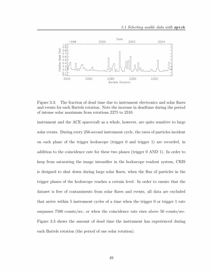
3.1 Selecting usable data with xpick
Figure 3.3: The fraction of dead time due to instrument electronics and solar flaresand events for each Bartels rotation. Note the increase in deadtime during the periodof intense solar maximum from rotations 2275 to 2310.
instrument and the ACE spacecraft as a whole, however, are quite sensitive to large
solar events. During every 256-second instrument cycle, the rates of particles incident
on each plane of the trigger hodoscope (trigger 0 and trigger 1) are recorded, in
addition to the coincidence rate for these two planes (trigger 0 AND 1). In order to
keep from saturating the image intensifier in the hodoscope readout system, CRIS
is designed to shut down during large solar flares, when the flux of particles in the
trigger planes of the hodoscope reaches a certain level. In order to ensure that the
dataset is free of contaminents from solar flares and events, all data are excluded
that arrive within 5 instrument cycles of a time when the trigger 0 or trigger 1 rate
surpasses 7500 counts/sec, or when the coincidence rate rises above 50 counts/sec.
Figure 3.3 shows the amount of dead time the instrument has experienced during
each Bartels rotation (the period of one solar rotation).
49

3.1 Selecting usable data with xpick
Figure 3.4: V Histograms of detector E3 from 28 Aug 1997 to 12 Aug 1999 at20, 30, and 45. The heights of 49V were lined up intentionally to demonstrate thedecrease in resolution with increasing angle. The fit mass resolutions for the threeplots are σ = 0.238, 0.251, and 0.265 amu respectively.
3.1.7 Angle cuts
As cosmic rays penetrate the silicon stack detectors, they Coulomb scatter and de-
viate slightly from the trajectory defined by analyzing the output of the hodoscope.
This effect becomes more and more significant with increasing zenith angle since the
amount of silicon penetrated increases. Properly analyzing data with low statistics
requires reaching a balance where the maximum allowable zenith angle permits the
acceptance of enough data without sacrificing the mass resolution to a great degree.
Where possible in this analysis, data with a zenith angle, θ, less than 30 are used,
however, when statistics are lower, data with θ < 45 are used. Figure 3.4 shows
how the number of events and mass resolution changes for different acceptance an-
gles. One can see from the figure that the mass resolution is reasonable even where
θ < 45.
50

3.2 The Dataset
3.2 The Dataset
3.2.1 Delineating time intervals
Once the data were selected and the aforementioned cuts and corrections were applied,
the data were separated into two time periods based on the 22-year solar cycle (see
Chapter 1.2). The period during which time the sun was relatively inactive, hereafter
referred to as solar minimum, extends from 28 August 1997 to 12 August 1999, and
includes Bartels Rotations 2239 through 2265. Solar minimum includes 715 days of
data during which time the CRIS livetime was found to be 548.87 days. The period
of high solar activity, hereafter referred to as solar maximum, extends from 2 July
2000 to 22 December 2003, and includes Bartels Rotations 2278 through 2324. Solar
maximum includes 1269 days of data, but with only 902.68 days of livetime. See
Figure 3.5.
3.2.2 Mass histograms
The data for each element were analyzed separately in detectors E2 through E8 and
the sum of all detectors. For data with Z < 17, the adjusted masses, corr mass,
were binned in bin sizes of 0.05 amu, whereas data with Z ≥ 17 were binned in
bin sizes of 0.1 amu. The stable and near-stable isotopes of each element were fit
to a multiple Gaussian curve using the Maximum-Likelihood method described in
Appendix A. In order to ensure that the mass values fitted were reasonably close
to the actual isotope integer values, first, the entire histogram was fitted and the
51

3.2 The Dataset
Figure 3.5: 27-day average intensity of 16O, 28Si, and 56Fe over the ACE lifetime.The shaded regions delineate the periods designated “solar minimum” and “solarmaximum” for this analysis. The energy ranges are 16O: 68 - 212 MeV/nucleon,28Si: 90 - 411 MeV/nucleon, and 56Fe: 126 - 566 MeV/nucleon. The 28Si intensityshown is multiplied by 1.8 for purposes of plotting.
mass resolution, σ, approximated. The dataset was then refitted including only data
between 2.5 σ below the lightest isotope and 2.5 σ above the heaviest isotope. Values
and uncertainties were thereby determined for the location (in amu) of the lightest
isotope, the peakspacing (amu) between adjacent isotopes, the mass resolution, σ, for
all isotopes, and the abundances of each isotope.
The histograms are approximately Gaussian in shape, but also contain a low-mass
tail visible to the left of the lightest stable isotope in each histogram plot. In most
cases, these are radioactive isotopes with short lifetimes that are not present in GCRs,
and so it is believed that these data arise from neutron stripping of the adjacent stable
isotope in the ∼ 0.442 g/cm2 of material above the Si detectors (Yanasak et al., 2001).
52

3.3 Histogram plots for solar minimum data
3.3 Histogram plots for solar minimum data
The following pages include plots of mass histograms for elements from B to Ni
(5 ≤ Z ≤ 28). The data included required an incident angle, θ ≤ 30 and were taken
during the period of solar minimum. In each figure, there are 7 plots that contain
data for cosmic rays that stop in detectors E2 through E8. The eighth plot shows
the sum of all seven of these detectors. In each plot, the mass resolution, σ, and the
energy range are included. The area between the dotted lines delineate which data
were fitted to a sum of Gaussian curves, except in the case of Co where the data have
such low statistics that particles between the lines have been counted. Spectral plots
for these isotopes can be found in Appendix D.
53

3.3 Histogram plots for solar minimum data
3.3.1 B histograms
Figure 3.6: Logarithmic histograms of B isotopes, θ < 30.
The B data include two isotopes at 10B and 11B, which are commonly known to
be secondary isotopes from interactions of C, N and O in the interstellar medium.
The logarithmic plots demonstrate clearly the tail to the left of 10B, most likely the
result of neutron stripping of 10B and 11B as they pass through the shielding material
above the hodoscope. The logarithmic plots are misleading; the peak-to-valley ratio
for this element is between ∼ 30 and ∼ 100. Note the poorer resolution and increased
noise in range 2 due to the absence of charge consistency cuts.
54

3.3 Histogram plots for solar minimum data
3.3.2 C histograms
Figure 3.7: Logarithmic histograms of C isotopes, θ < 30.
One of the most abundant elements in the GCRs heavier than He, this analysis of
C includes the two isotopes, 12C and 13C. Note also here the tail to the left of the 12C
peak caused by neutron stripping in the shielding material. The radioactive isotope
14C, with a laboratory half-life of 5700 years, decays almost completely on galactic
time scales and is therefore left out of this analysis.
55

3.3 Histogram plots for solar minimum data
3.3.3 N histograms
Figure 3.8: Logarithmic histograms of N isotopes, θ < 30.
The N data include two isotopes at 14N and 15N. The logarithmic plots demon-
strate clearly the tail to the left of 14N, most likely the result of neutron stripping of
14N and 15N as they pass through the shielding material above the hodoscope. Note
the poorer resolution and increased noise in range 2 due to the absence of charge
consistency cuts.
56

3.3 Histogram plots for solar minimum data
3.3.4 O histograms
Figure 3.9: Logarithmic histograms of O isotopes, θ < 30.
The O data include three isotopes: 16O, 17O and 18O. Oxygen-16 is one of the
most abundant isotopes in the cosmic rays heavier than He and is almost entirely
primary in origin.
57
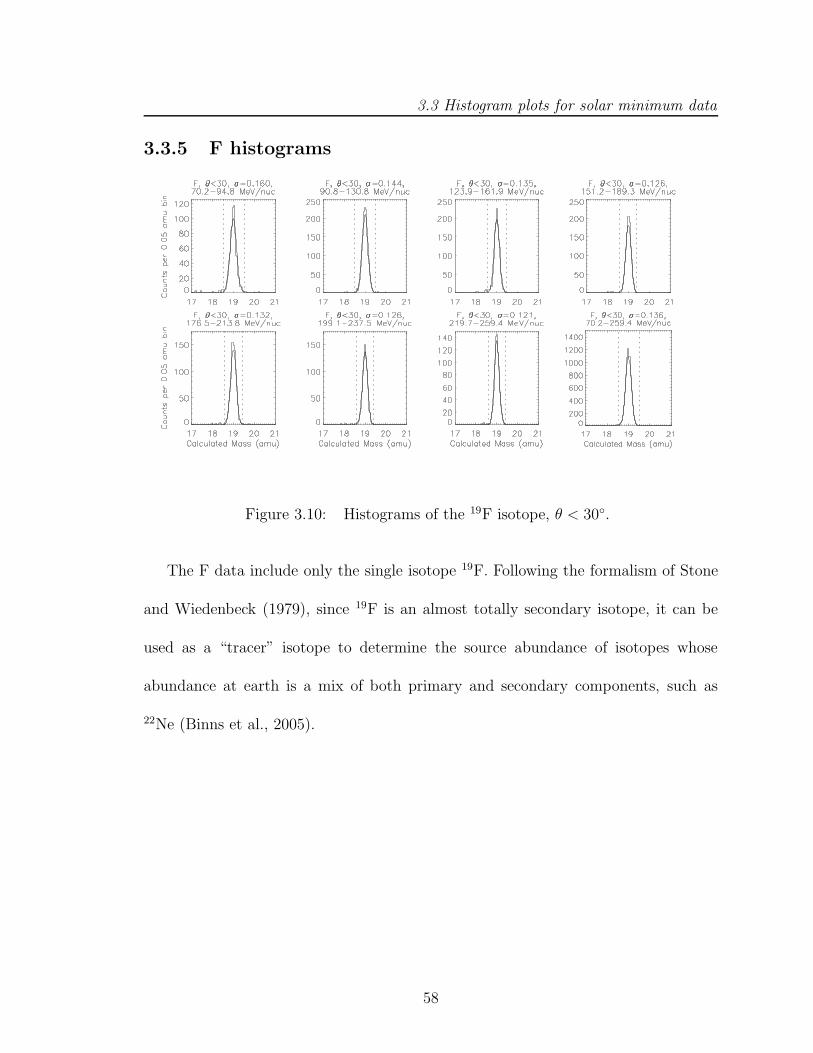
3.3 Histogram plots for solar minimum data
3.3.5 F histograms
Figure 3.10: Histograms of the 19F isotope, θ < 30.
The F data include only the single isotope 19F. Following the formalism of Stone
and Wiedenbeck (1979), since 19F is an almost totally secondary isotope, it can be
used as a “tracer” isotope to determine the source abundance of isotopes whose
abundance at earth is a mix of both primary and secondary components, such as
22Ne (Binns et al., 2005).
58
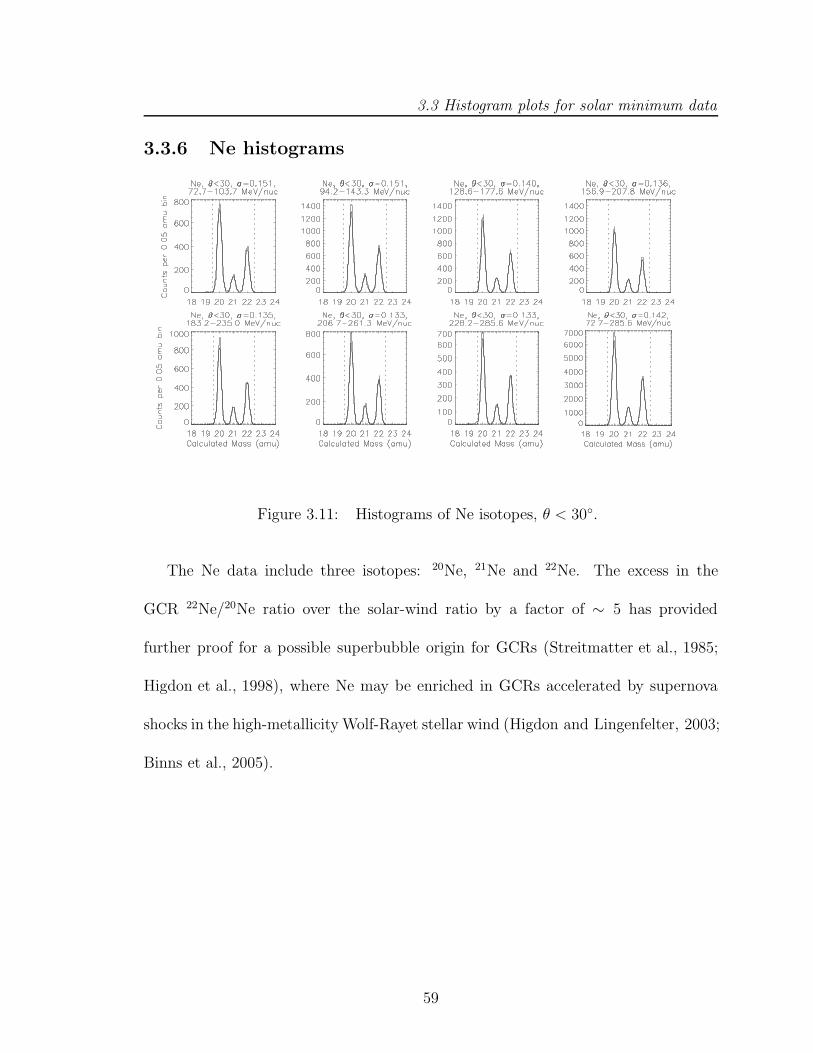
3.3 Histogram plots for solar minimum data
3.3.6 Ne histograms
Figure 3.11: Histograms of Ne isotopes, θ < 30.
The Ne data include three isotopes: 20Ne, 21Ne and 22Ne. The excess in the
GCR 22Ne/20Ne ratio over the solar-wind ratio by a factor of ∼ 5 has provided
further proof for a possible superbubble origin for GCRs (Streitmatter et al., 1985;
Higdon et al., 1998), where Ne may be enriched in GCRs accelerated by supernova
shocks in the high-metallicity Wolf-Rayet stellar wind (Higdon and Lingenfelter, 2003;
Binns et al., 2005).
59
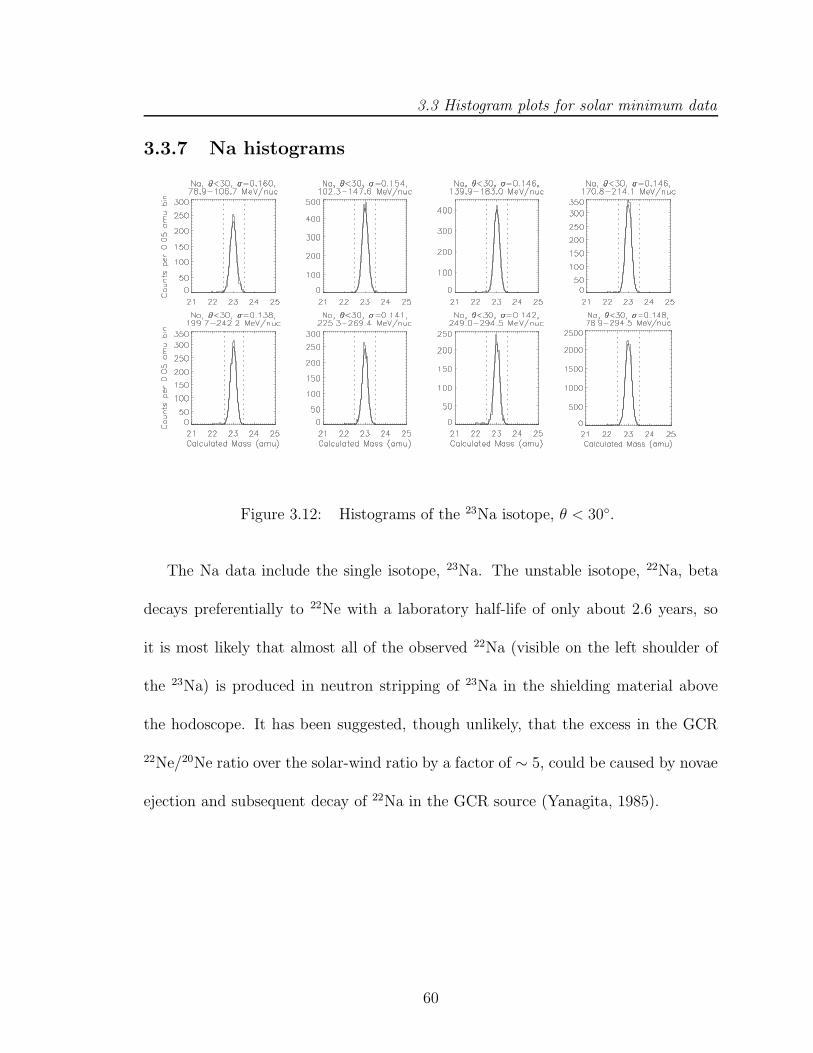
3.3 Histogram plots for solar minimum data
3.3.7 Na histograms
Figure 3.12: Histograms of the 23Na isotope, θ < 30.
The Na data include the single isotope, 23Na. The unstable isotope, 22Na, beta
decays preferentially to 22Ne with a laboratory half-life of only about 2.6 years, so
it is most likely that almost all of the observed 22Na (visible on the left shoulder of
the 23Na) is produced in neutron stripping of 23Na in the shielding material above
the hodoscope. It has been suggested, though unlikely, that the excess in the GCR
22Ne/20Ne ratio over the solar-wind ratio by a factor of ∼ 5, could be caused by novae
ejection and subsequent decay of 22Na in the GCR source (Yanagita, 1985).
60

3.3 Histogram plots for solar minimum data
3.3.8 Mg histograms
Figure 3.13: Histograms of Mg isotopes, θ < 30.
The Mg data include the three isotopes, 24Mg, 25Mg and 26Mg, all of which have a
significant primary component. The ratios of 25Mg/24Mg and 26Mg/24Mg are gener-
ally consistent with solar-system abundances (Webber et al., 1997). This fact has pro-
vided proof against such GCR source models as the supermetallicity model of Woosley
and Weaver (1981), which predicted an enhancement in these ratios in the GCRs over
the solar-system abundances. Recent modifications to the Wolf-Rayet model includ-
ing better cross section data have reconciled this difference (Casse and Paul, 1982;
Meynet et al., 2001; Binns et al., 2005).
61

3.3 Histogram plots for solar minimum data
3.3.9 Al histograms
Figure 3.14: Logarithmic histograms of Al isotopes, θ < 30.
The Al data include two isotopes: 26Al and 27Al. The unstable isotope, 26Al, beta
decays to 26Mg with a half-life of 7.1 × 10⁵ years. The abundance of this secondary
radionuclide has been used as a propagation clock in determining the mean galactic
confinement time of 15.0 ± 1.6 Ma (Yanasak et al., 2001).
62

3.3 Histogram plots for solar minimum data
3.3.10 Si histograms
Figure 3.15: Histograms of Si isotopes, θ < 30.
The Si data include three isotopes: 28Si, 29Si and 30Si. Silicon-28 is one of the most
abundant heavy isotopes and is almost totally primary in the cosmic rays. As with the
heavy Mg isotopes, recent measurements of the 29Si/28Si and 30Si/28Si ratios that are
comparable to solar-system values disagree with the predictions of the Woosley and
Weaver supermetallicity model, but are in good agreement with recent modifications
to the Wolf-Rayet model (Meynet et al., 2001; Binns et al., 2005).
63

3.3 Histogram plots for solar minimum data
3.3.11 P histograms
Figure 3.16: Histograms of the 31P isotope, θ < 30.
The data for P contain the single stable isotope 31P. Phosphorus is mostly sec-
ondary in the cosmic rays, owing mostly to spallation of 32S, 40Ar and 40Ca.
64

3.3 Histogram plots for solar minimum data
3.3.12 S histograms
Figure 3.17: Histograms of S isotopes, θ < 30.
The S data include three isotopes: 32S, 33S and 34S. The stable isotope, 36S is rela-
tively rare and has been excluded from this analysis. As with Mg and Si, the cosmic-
ray source ratios of 34S/32S and 33S/32S are found to agree with solar-system values,
perhaps with a slight enhancement of the latter ratio in the GCRs (Thayer, 1997).
65

3.3 Histogram plots for solar minimum data
3.3.13 Cl histograms
Figure 3.18: Histograms of Cl isotopes, θ < 30.
The Cl data include three isotopes: 35Cl, 36Cl and 37Cl. Argon-37 decays to
37Cl by electron-capture with a laboratory half-life of 35.0 days. Chlorine-36, which
beta decays almost totally to 36Ar in the cosmic rays with a laboratory half-life of
3.01× 10⁵ years, has been used in determining the mean containment time for GCRs
in the Galaxy (Yanasak et al., 2001).
66

3.3 Histogram plots for solar minimum data
3.3.14 Ar histograms
Figure 3.19: Histograms of Ar isotopes, θ < 30.
The Ar data include four isotopes: 36Ar, 37Ar, 38Ar and 40Ar. The isotope 39Ar
beta decays to 39K with a laboratory half-life of only 269 years, so it is absent in
the GCRs. Argon-36 is the beta-decay product of 36Cl, 37Ar decays to 37Cl only by
electron-capture with a laboratory half-life of 35 days.
67

3.3 Histogram plots for solar minimum data
3.3.15 K histograms
Figure 3.20: Histograms of K isotopes, θ < 30.
The K data include three isotopes: 39K, 40K and 41K. Although 40K decays both to
40Ca and 40Ar, the half-life of 1.27×10⁹ years is about two orders of magnitude longer
than the cosmic-ray lifetime, and so 40K is present in the cosmic rays. Potassium-41
is the electron-capture decay product of 41Ca.
68

3.3 Histogram plots for solar minimum data
3.3.16 Ca histograms
Figure 3.21: Logarithmic histograms of Ca isotopes, θ < 30.
The Ca data include five isotopes: 40Ca, 41Ca, 42Ca, 43Ca, 44Ca, 46Ca and 48Ca.
Although the stable isotopes 46Ca and 48Ca are present in the cosmic rays, they are
much less abundant than the other calcium isotopes and have therefore been left out
of the Gaussian peak fitting. The 46Ca and 48Ca peaks are sufficiently separated
that their abundances can be easily estimated by counting. Calcium-40 is estimated
to be about 98% of primary origin, whereas the heavier isotopes are less than 10%
primary (Stone and Wiedenbeck, 1979). Calcium-44 is produced mostly as the beta-
decay product of 44Sc, which is in turn, the electron-capture decay product of 44Ti.
Calcium-41 decays to 41K by electron capture with a half-life of 1.03 × 10⁵ years.
69

3.3 Histogram plots for solar minimum data
3.3.17 Sc histograms
Figure 3.22: Histograms of the 45Sc isotope, θ < 30.
The data for Sc contain the single stable isotope 45Sc. Scandium-45 is the lightest
isotope in the group that will hereafter be referred to as the Fe secondaries. The
isotope is almost entirely secondary in origin, produced mostly from interactions of
56Fe with hydrogen atoms in the interstellar medium.
70

3.3 Histogram plots for solar minimum data
3.3.18 Ti histograms
Figure 3.23: Histograms of Ti isotopes, θ < 30.
The six isotopes of Titanium, 44Ti, 46Ti, 47Ti, 48Ti, 49Ti and 50Ti, are remarkably
well-resolved in the CRIS data. Titanium is mostly secondary in origin, owing in
large part to spallation of 56Fe in the interstellar medium. Titanium-44 decays only
by electron-capture to 44Sc with a half-life of 67 years. Scandium-44 beta decays
quickly (2.44 days) to 44Ca. All heavier isotopes are stable, but it is important to
note that 49Ti is the electron-capture decay product of 49V. Titanium-45 is extremely
short-lived, beta-decaying to 45Sc with a half-life of only about 3 hours.
71

3.3 Histogram plots for solar minimum data
3.3.19 V histograms
Figure 3.24: Histograms of V isotopes, θ < 30.
The V data include three isotopes: 49V, 50V and 51V. The cosmic-ray V isotopes
have almost no primary component and are involved to a large degree in electron-
capture decay. At low enough energies for electron attachment, 49V decays by electron
capture to 49Ti with a laboratory half-life of 337 days. Vanadium-51 is the electron-
capture-decay product of 51Cr. The isotope 50V is stable in the cosmic rays.
72

3.3 Histogram plots for solar minimum data
3.3.20 Cr histograms
Figure 3.25: Histograms of Cr isotopes, θ < 30.
The Cr data include five isotopes: 50Cr, 51Cr, 52Cr, 53Cr and 54Cr. Like the
other Fe secondary elements, the isotopes of Cr are mostly created by spallation of
56Fe in the interstellar medium. Chromium-51 electron-capture decays to 51V with
a laboratory half-life of 27.7 days. The other isotopes are stable. Although 53Cr
is the electron-capture decay product of 53Mn, it is difficult to study due to its long
decay half-life. Chromium-54 has a small primary component and is also the electron-
capture decay product of 54Mn.
73

3.3 Histogram plots for solar minimum data
3.3.21 Mn histograms
Figure 3.26: Histograms of Mn isotopes, θ < 30.
The Mn data include three isotopes: 53Mn, 54Mn and 55Mn. Manganese-53 decays
by electron-capture to 53Cr with a laboratory half-life of 3.6×10⁶ years, too long com-
pared to the time scale for an electron to be stripped from the nucleus to be useful in
electron-capture-decay studies. Manganese-54 decays through electron-capture decay,
β+- and β−-decay. Although the half-life for electron-capture decay (312 days) is much
lower than those for both β+- and β−-decay, at high enough energies electron-capture
decay is unlikely. With better data for these beta-decay half-lives, 54Mn could be
used to probe the residence time of cosmic-rays in the Galaxy (Yanasak et al., 2001).
Manganese-55 is the electron-capture decay product of 55Fe.
74

3.3 Histogram plots for solar minimum data
3.3.22 Fe histograms
Figure 3.27: Logarithmic histograms of Fe isotopes, θ < 30.
The Fe data include the five isotopes 54Fe, 55Fe, 56Fe, 57Fe, 58Fe and 60Fe. Although
60Fe is a long-lived radionuclide (it beta decays to 60Co with a half-life of 1.5 Ma), it
is extremely rare and has therefore been omitted from this analysis. Iron-55 decays
by electron-capture to 55Mn with a laboratory half-life of 2.73 years. Iron-56 is the
most abundant nuclide heavier than 28Si in the cosmic rays, and it is almost entirely
primary in origin, produced as the electron-capture-decay product of 56Ni after the
stellar nucleosynthesis reaction 28Si +28 Si →56Ni. Iron-57 is the electron-capture
decay product of 57Co.
75
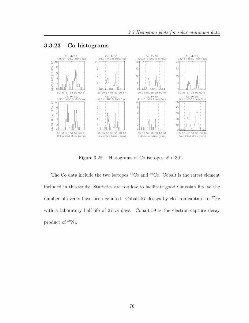
3.3 Histogram plots for solar minimum data
3.3.23 Co histograms
Figure 3.28: Histograms of Co isotopes, θ < 30.
The Co data include the two isotopes 57Co and 59Co. Cobalt is the rarest element
included in this study. Statistics are too low to facilitate good Gaussian fits, so the
number of events have been counted. Cobalt-57 decays by electron-capture to 57Fe
with a laboratory half-life of 271.8 days. Cobalt-59 is the electron-capture decay
product of 59Ni.
76

3.3 Histogram plots for solar minimum data
3.3.24 Ni histograms
Figure 3.29: Logarithmic histograms of Ni isotopes, θ < 30.
The Ni data include the four isotopes 58Ni, 60Ni, 61Ni and 62Ni. Nickel-59 is almost
entirely primary, the stable nuclide to which all mass-59 nuclei with Z ≥ 28 finally de-
cay following a supernova explosion. Decaying only by electron-capture to 59Co with
a half-life of 76,000 years, its absence has been used to provide evidence for a delay be-
tween nucleosynthesis and acceleration in the cosmic rays (Wiedenbeck et al., 1999).
Although 64Ni is a stable isotope, it is relatively scarce and has been omitted from
this study.
77

3.4 Fragmentation corrections
3.4 Fragmentation corrections
Most nuclei that fragment during their journey through the CRIS instrument are elim-
inated by the charge-consistency cuts described in §3.1.2. It is important, however,
that these fragmented nuclei be taken into account when calculating an abundance
for a certain isotope at the top of the instrument.
The probability for a nucleus to survive spallation when passing through a given
range, R, of silicon can be found
ηspall(E,Zi, Ai) = exp
[
−R(E,Zi, Ai)
Λ(Ai)
]
, (3.4)
where R(E,Zi, Ai) is the total range as measured in g/cm2 of silicon in the instru-
ment (including all materials above the silicon stack detectors) for an element with
charge Zi, mass number Ai and average energy E as measured in MeV/nucleon, at
the average angle for all incident particles with θ ≤ 30. The mean free path for
fragmentation of the nucleus in the instrument, Λ(Ai), is then found
Λ(Ai) =AT
NAσ(Ai, AT ), (3.5)
where AT = 28 for silicon and NA is Avogadro’s number. Westfall (1979) has shown
that the a good approximation of the cross section of interaction between a nucleus
of mass Ai on a target nucleus AT is
σ(Ai, AT ) = πr02(Ai
13 + AT
13 − b)2. (3.6)
Following the method of Yanasak (2001), r0 = 1.47 fm and b = 1.12. Probabilities of
surviving spallation vary from about 96% for Boron in detector E2 to 61% for Nickel
78

3.5 SOFT Efficiency corrections
in detector E8. Since an uncertainty of as much as 10% in either the cross section
or range in Si will result in a much smaller uncertainty in the spallation survival
probability, following the formalism of George et al. (2005), I have conservatively
attributed a possible 3% uncertainty to this factor.
3.5 SOFT Efficiency corrections
The Scintillating Optical Fiber Trajectory system describes the trajectories of par-
ticles in CRIS very efficiently, and any corrections that need to be made are quite
small, especially for large Z. Most of the uncertainty arises for a nucleus that passes
between fibers in the cladding region of the hodoscope, resulting in a weak signal from
knock-on electrons, instead of a strong signal from energy deposited by the nucleus
itself. The probability that an event of a given Z can be detected by the SOFT system
was found by isolating the events for that element that could be characterized solely
by their signals in detectors E4 through E8 and determining what fraction of those
had good trajectories in SOFT. These efficiencies range from about 86% for Boron in
detector E8 to better than 99% for all elements with Z ≥ 17 in all detectors.
As with the uncertainty for the spallation correction, the uncertainty on the SOFT
efficiency is also quite small. Owing mostly to the systematics of the method used
to define these efficiencies, a 2% uncertainty is attributed to the SOFT efficiency
(George et al., 2005).
79

3.6 Abundance ratios
3.6 Abundance ratios
The corrections described in §3.4 and §3.5 are important when calculating abundance
ratios of two different isotopes and the energy spectrum of a single isotope. For
abundance ratios, the number of events, N , of an isotope in question must be adjusted
by a factor, f , to a given standard energy range due to the differences in the range-
energy relation and in the spectral shapes of different isotopes (see Appendix B).
This standard energy range is normally taken to be the energy range of the lightest or
lowest-Z isotope in question. In addition to the range-energy and spectral corrections,
the adjusted abundance, N ′ = fN , of each isotope is adjusted to N ′′ such that
N ′′ =fN
ηspall · ηSOFT
, (3.7)
where ηspall is the probability of surviving spallation and ηSOFT is the SOFT detection
efficiency.
The uncertainty on the measured abundance σN (as described in Appendix A) is
adjusted by the normalization factor from Appendix B. This normalized uncertainty
σN ′ becomes one of a number of uncertainties on the actual observed abundance. The
total uncertainty σN ′′ can then be found
σN ′′
N ′′ =
√
(σN
N
)2
+
(
σspall
ηspall
)2
+
(
σSOFT
ηSOFT
)2
, (3.8)
where σspall and σSOFT are the uncertainties on the probability of surviving spallation
in the instrument and on the SOFT efficiency, as discussed in §3.4 and §3.5. Adjusted
abundance ratios can then be found easily with resultant uncertainties derived in the
80

3.7 Spectral calculations
normal way (Equation 3.8).
3.7 Spectral calculations
The differential energy spectrum,(
dJdE
)
i, for a given isotope i, as presented in Ap-
pendix D, is calculated
(
dJ
dE
)
i
=Ni
Γi · t · ηspall,i · ηSOFT
, (3.9)
where Ni is the measured abundance as discussed in Appendix A, Γi =∫
AΩdE is
the geometry factor, as discussed in Appendix C, and t is the livetime, as discussed
in §3.2.1. The resulting uncertainty σ( dJdE )
i
is then found
σ( dJdE )
i
=
(
dJ
dE
)
i
·√
(
σNi
Ni
)2
+
(
σΓi
Γi
)2
+
(
σspall,i
ηspall,i
)2
+
(
σSOFT
ηSOFT
)2
. (3.10)
81

Chapter 4
CRIS Measurements ofElectron-Capture-Decay Isotopes
This chapter will discuss the principles of electron-capture (EC) decay and the models
used to evaluate the role that it plays in the propagation of GCRs. The EC daughter-
to-parent abundance ratios measured by CRIS will be presented during the periods
of solar minimum and solar maximum.
4.1 Electron-capture decay
The process of electron-capture decay (also known as K-capture decay) involves the
capture of an electron from the cloud surrounding the atomic nucleus. This process
most often occurs in heavier nuclei that have larger nuclear radii and whose K-shell
electron orbits are more compact. Since the radial wave function of a K-shell electron
has a maximum at the center of the nucleus, there is a finite probability that an
electron may find itself inside the nucleus and precipitate the reaction
p + e− → n + νe. (4.1)
82
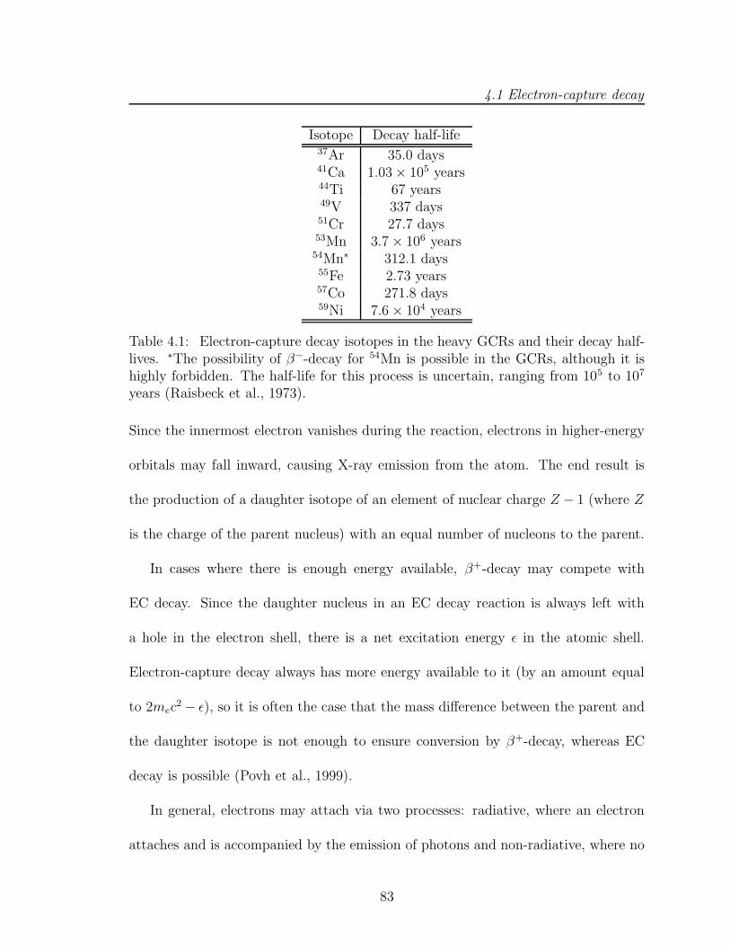
4.1 Electron-capture decay
Isotope Decay half-life37Ar 35.0 days41Ca 1.03 × 10⁵ years44Ti 67 years49V 337 days51Cr 27.7 days53Mn 3.7 × 10⁶ years54Mn∗ 312.1 days55Fe 2.73 years57Co 271.8 days59Ni 7.6 × 10⁴ years
Table 4.1: Electron-capture decay isotopes in the heavy GCRs and their decay half-lives. ∗The possibility of β−-decay for 54Mn is possible in the GCRs, although it ishighly forbidden. The half-life for this process is uncertain, ranging from 105 to 107
years (Raisbeck et al., 1973).
Since the innermost electron vanishes during the reaction, electrons in higher-energy
orbitals may fall inward, causing X-ray emission from the atom. The end result is
the production of a daughter isotope of an element of nuclear charge Z − 1 (where Z
is the charge of the parent nucleus) with an equal number of nucleons to the parent.
In cases where there is enough energy available, β+-decay may compete with
EC decay. Since the daughter nucleus in an EC decay reaction is always left with
a hole in the electron shell, there is a net excitation energy ε in the atomic shell.
Electron-capture decay always has more energy available to it (by an amount equal
to 2mec2 − ε), so it is often the case that the mass difference between the parent and
the daughter isotope is not enough to ensure conversion by β+-decay, whereas EC
decay is possible (Povh et al., 1999).
In general, electrons may attach via two processes: radiative, where an electron
attaches and is accompanied by the emission of photons and non-radiative, where no
83
4.2 Electron-capture decay in GCRs
photon emission accompanies the electron attachment. The non-radiative process is
much less likely for heavier, high-energy nuclei and so it can be essentially ignored
for the purposes of this study (Niebur, 2001).
4.2 Electron-capture decay in GCRs
4.2.1 Electron attachment
Electron-capture decay in GCRs is notably different than other forms of nuclear
decay, due to the extreme energy dependence of electron attachment. Galactic cosmic
rays secondaries are created by spallation already propagating at several hundred
MeV/nucleon in the interstellar medium, and are therefore born entirely stripped of
all of their orbital electrons. Because of this, electron-capture-decay isotopes at these
energies are effectively stable. In addition, at lower energies where it becomes easier to
attach an electron, the timescale to strip this electron is normally significantly longer
than the decay half-life, as can be seen in Figure 4.1. The result is that electron-
capture-decay isotopes with short half-lives that attach an electron will almost always
decay before being stripped of this electron. Preliminary work by Raisbeck et al.
(1975) and Letaw et al. (1985) demonstrated that substantial electron-capture decay
should occur in cosmic rays with energies below about 500 MeV/nucleon.
Because electron-capture decay effectively “turns on” at a given energy for a given
isotope, the correct determination of the cross section for electron attachment is of
great importance when modeling the effects of EC decay in GCRs. The relativistic
84

4.2 Electron-capture decay in GCRs
first-order Born approximation has been shown to work well when calculating the
attachment cross section. More detail, including a derivation of this approximation
from the principles of the inverse process of photoionization can be found in Wilson
(1978) and Crawford (1979).
More recently, it has been shown using energetic nuclei in gas targets that it may
be possible to calculate the cross section of electron attachment based on a nucleus’
adiabaticity (Stohlker et al., 1995). The adiabaticity parameter, η is a measure of
the energy, E of the nucleus versus EIP , the ionization potential of the first K-shell
electron and is given by
η =E
EIP
me
mN
(4.2)
where mN is the mass of the nucleus in question. When plotting the electron-
attachment cross section, σEC versus ν, the relation obeys a power law
σEC ∝ ηγ (4.3)
with γ ∼ −2. In general, this determination of the attachment cross section agrees
well with the Born approximation (Niebur, 2001).
4.2.2 Electron stripping
The Bohr formula for the stripping cross section for electrons as modified by Wilson
(1978) for the effects of ionization from distant collisions is given by
σstrip =4πa0
2α2
ZN2β2
(Zt2 + Zt)
(
C1
[
ln
(
4β2γ2
C2ZN2α2
)
− β2
])
(4.4)
85

4.3 CRIS observations of electron-capture decay
where ZN is the charge of the nucleus in question, a0 is the classical electron radius
(0.052918 nm), α is the fine-structure constant, Zt is the charge of the target nucleus,
β and γ are the velocity and Lorentz factor of the nucleus in question and C1 and
C2 are 0.285 and 0.048 respectively. For most isotopes in Table 4.1, the time scale
for stripping an electron far excedes the EC decay half-life. For example, an 37Ar
nucleus propagating at 100 MeV/nucleon will have an electron stripped in ∼ 5400
years, whereas with one electron already attached, it will decay in only 70 days (twice
the half-life in which there are two K-shell electrons attached). A 57Co nucleus at
100 MeV will lose an electron after ∼14,000 years versus a decay life of less than a
year. Figure 4.1 details how the process of electron attachment competes with other
loss mechanisms and how decay competes with stripping of nuclei with one attached
electron. In the cases of 41Ca, 53Mn, and 59Ni, it is evident from Figure 4.1 that the
competition between EC decay and stripping make this situation more complex since
most low-energy nuclei will not decay before being stripped of their attached electron.
4.3 CRIS observations of electron-capture decay
Raisbeck et al. (1973) was the first to note the possibility of using EC decay secondary
isotopes as a probe of energy loss in GCRs in the heliosphere. The energy dependence
of electron-capture decay in secondary nuclei can shed light on the propagation of
cosmic rays through the ISM and the heliosphere, since they are born in the ISM
already propagating at high energies. Primary electron-capture decay isotopes such
86

4.3 CRIS observations of electron-capture decay
Figure 4.1: The time scales of various processes for 51Cr with a hydrogen atomdensity of 0.34 atoms/cm3. The label “other losses” refers to nuclei which fragmentinto lighter atoms or escape from the Galaxy. Note the extreme energy dependence ofelectron attachment, but that when the time scale becomes reasonable to attach anelectron, decay will almost inevitably win out over stripping, fragmentation or escape(Wiedenbeck, 2003b).
as 59Ni, on the other hand, have been shown to decay entirely before being accelerated
and hence give little information about energy-changing processes between the source
and the detector, but rather can be used to set a lower limit on the time delay between
nucleosynthesis and acceleration (Wiedenbeck et al., 1999).
The CRIS instrument is the first of its kind with adequate mass resolution and
statistics in the sub-Fe regime to be able to conduct this kind of study. Previously,
Soutoul et al. (1998) attempted a study the relative abundances of 49V and 51V
87

4.3 CRIS observations of electron-capture decay
Figure 4.2: 51V/51Cr with and without EC decay. The solid and dashed lines showthe mass-51 electron-capture decay abundance ratio in the ISM and at 1 AU usingthe leaky-box model discussed in §5. The dotted and dot-dashed lines show the sameratio with EC decay turned off. Note the “smearing” of the interstellar spectrum at1 AU due to solar modulation. There is no energy-dependent feature if EC decay isturned off: the abundance ratio remains essentially unchanged from what it is at highenergies where electron-capture is prohibited (Wiedenbeck, 2003b).
from a combination of Voyager and ISEE 3 data in hopes of measuring the effects
of the EC decay of 49V and 51Cr, but poor isotopic resolution and limited statis-
tics prohibited a detailed study. These same EC decay reactions were studied with
data from the Ulysses spacecraft, but again, limited statistics hampered the results
(Connell and Simpson, 1999; Connell, 2001).
Comparison of the abundance ratios of the daughter to the parent gives the most
information about the energy dependence of an electron-capture-decay reaction in the
88

4.3 CRIS observations of electron-capture decay
GCRs. At the lowest energies in CRIS where the cross section for electron attachment
is much higher, one would expect that most of the parent isotope would have decayed
to the daughter isotope, and therefore observe a higher daughter-to-parent ratio. At
higher energies, one would expect that little or none of the parent has decayed, and
that the abundance ratio should be lower and flatter with respect to energy than at
lower energies. Were one able to observe this ratio in the ISM, one would expect the
ratio to increase greatly at lower energies.
Inside the heliosphere during periods of solar minimum where particles suffer a
decrease in intensity and a reduction in energy, the abundance ratio should maintain
this energy-dependent feature, albeit less pronounced than in the ISM. During periods
of solar maximum, however, one would presume that particles propagating at high
energies in the interstellar medium would have suffered a more significant reduction in
intensity and energy than during solar minimum as they propagated in the heliosphere
toward Earth. As a result, in the CRIS energy range, this abundance ratio should be
lower and essentially featureless as it is at much higher energies in the ISM.
Figure 4.2 shows how the abudance ratio of the daughter to the parent in the EC
decay reaction of 51Cr is modulated by the sun at 1 AU. Notice that if EC decay
is turned off, the abundance ratio remains constant with energy, as it does at the
highest energies where EC decay cannot occur.
The next sections will present the daughter-to-parent abundance ratios for the EC
decay isotopes in Table 4.1 (except 59Ni where the parent has decayed entirely). A
qualitative assessment of the usefulness of the abundance ratios as a probe of solar
89

4.3 CRIS observations of electron-capture decay
modulation will also be discussed. It will be shown that the EC decay isotopes 49V
and 51Cr are the most useful for measuring the effects of solar modulation.
90

4.3 CRIS observations of electron-capture decay
4.3.1 37Ar → 37Cl
Argon-37 decays to 37Cl with a laboratory half-life of only 35.0 days. Although the
individual isotopes of Ar and Cl are well-resolved, as can be seen in Figures 3.18 and
3.19, due to the extremely limited statistics available when accepting only events with
zenith angle, θ < 30, I have chosen to extend the angle of acceptance to 45 for this
study. Table 4.2 gives the results of fitting the mass histograms for 37Ar and 37Cl to
a multiple Gaussian and correcting for the effects of spallation, SOFT efficiency and
spectral differences between the two isotopes.
Provided 37Ar at low energies attaches an electron, it will decay to 37Cl much
quicker than it will be stripped of this electron. It is evident from Figure 4.3, however,
that there is no obvious enhancement of 37Cl at low energies as one might expect.
This is perhaps due, in part, to the low statistics and somewhat large error bars for
these data points. Additionally, as demonstrated in §4.2.1, for 3718Ar, the cross section
for electron attachment does not become large enough to compete with other loss
mechanisms until below about 100 MeV/nucleon, giving rise to an enhancement in
37Cl for energies below that in which CRIS is sensitive.
The data look similar during periods of solar minimum and solar maximum, and
so ultimately, little can be learned about the effects of solar modulation from the EC
decay of 37Ar. Table 4.3 presents the values of 37Cl/37Ar at solar minimum and solar
maximum.
91

4.3 CRIS observations of electron-capture decay
37 Ar at solar minimum, θ < 45Fit Spallation Range-Energy Adjusted
Detector Abundance Correction Adj. Factor AbundanceE2 307.93 ± 18.62 1.073 ± 0.032 0.882 293.88 ± 20.69E3 550.42 ± 24.71 1.123 ± 0.034 0.893 557.25 ± 32.09E4 460.28 ± 22.35 1.194 ± 0.036 0.904 501.14 ± 30.31E5 336.20 ± 19.12 1.269 ± 0.038 0.911 392.30 ± 26.41E6 314.53 ± 18.42 1.346 ± 0.040 0.917 392.04 ± 26.96E7 239.59 ± 15.92 1.428 ± 0.043 0.922 318.36 ± 24.07E8 203.75 ± 14.87 1.517 ± 0.046 0.927 289.09 ± 23.53
37 Ar at solar maximum, θ < 45Fit Spallation Range-Energy Adjusted
Detector Abundance Correction Adj. Factor AbundanceE2 232.27 ± 16.09 1.073 ± 0.032 0.892 224.22 ± 17.51E3 375.26 ± 20.47 1.123 ± 0.034 0.896 381.05 ± 24.92E4 331.03 ± 19.09 1.194 ± 0.036 0.900 358.84 ± 24.40E5 289.81 ± 18.00 1.269 ± 0.038 0.902 334.89 ± 24.05E6 208.94 ± 15.24 1.346 ± 0.040 0.905 256.81 ± 20.89E7 180.71 ± 14.01 1.428 ± 0.043 0.906 235.96 ± 20.18E8 169.42 ± 13.38 1.517 ± 0.046 0.908 235.51 ± 20.45
————————————————————————37 Cl at solar minimum, θ < 45
Fit Spallation Range-Energy AdjustedDetector Abundance Correction Adj. Factor Abundance
E2 177.89 ± 13.41 1.073 ± 0.032 1.000 192.53 ± 16.09E3 319.75 ± 18.07 1.123 ± 0.034 1.000 362.34 ± 24.28E4 256.91 ± 16.15 1.194 ± 0.036 1.000 309.51 ± 22.43E5 226.82 ± 15.12 1.269 ± 0.038 1.000 290.41 ± 22.01E6 171.13 ± 13.21 1.346 ± 0.040 1.000 232.50 ± 19.81E7 128.13 ± 11.41 1.428 ± 0.043 1.000 184.58 ± 17.73E8 126.48 ± 11.39 1.517 ± 0.046 1.000 193.62 ± 18.78
37 Cl at solar maximum, θ < 45Fit Spallation Range-Energy Adjusted
Detector Abundance Correction Adj. Factor AbundanceE2 165.50 ± 12.96 1.073 ± 0.032 1.000 179.13 ± 15.45E3 254.18 ± 16.09 1.123 ± 0.034 1.000 288.03 ± 20.99E4 225.44 ± 15.08 1.194 ± 0.036 1.000 271.59 ± 20.64E5 183.45 ± 13.62 1.269 ± 0.038 1.000 234.88 ± 19.39E6 149.48 ± 12.27 1.346 ± 0.040 1.000 203.08 ± 18.21E7 139.59 ± 11.85 1.428 ± 0.043 1.000 201.07 ± 18.55E8 128.21 ± 11.41 1.517 ± 0.046 1.000 196.27 ± 18.84
Table 4.2: Measurements and corrections to the abundances of 37Ar and 37Cl duringsolar minimum and solar maximum. The spallation correction is found using themethod discussed in §3.4. Argon-37 has been spectrally adjusted to the 37Cl energyrange as discussed in Appendix B. The adjusted abundance includes an additionalSOFT efficiency correction factor of 1.009 ± 0.020 as discussed in §3.5.
92

4.3 CRIS observations of electron-capture decay
37Cl/37Ar at solar minimum, θ < 45
EnergyDetector [MeV/nuc] Ratio
E2 118.40 0.655 ± 0.072E3 160.20 0.649 ± 0.057E4 207.72 0.617 ± 0.058E5 248.65 0.739 ± 0.075E6 285.13 0.592 ± 0.065E7 318.39 0.580 ± 0.071E8 352.27 0.670 ± 0.085
37Cl/37Ar at solar maximum, θ < 45
EnergyDetector [MeV/nuc] Ratio
E2 118.40 0.799 ± 0.093E3 160.20 0.756 ± 0.074E4 207.72 0.757 ± 0.077E5 248.65 0.701 ± 0.077E6 285.13 0.791 ± 0.096E7 318.39 0.852 ± 0.107E8 352.27 0.833 ± 0.108
Table 4.3: Values of 37Cl/37Ar at solar minimum and solar maximum.
Figure 4.3: 37Cl/37Ar at solar minimum and maximum.
93

4.3 CRIS observations of electron-capture decay
4.3.2 41Ca → 41K
The decay of 41Ca to 41K is somewhat different than the others mentioned in Table
4.1 in that its decay half-life of ∼ 105 years is on a longer time scale than that
for stripping at nominal electron attachment energies. It must be therefore assumed
that 41Ca is effectively stable in the GCRs and that the observed 41K is produced in
a small amount at the source and in larger amounts by spallation of heavier nuclei
during propagation.
As can be seen from Figure 4.4, the 41Ca isotope is well-resolved. Since it is
succeeded by the more abundant isotope 42Ca, it is most certain that some of the 41Ca
is produced by neutron-stripping of 42Ca in the CRIS shielding material above the
hodoscope. According to Yanasak (2001), an isotope will be enhanced by 0.7+0.5−0.7%
of the abundance of the next heaviest neighbor due to this effect. Including this
correction would increase the abundance of 41Ca by less than 1%. Since this correction
is small compared to all other corrections listed in Table 4.4, I have omitted it from
this study.
Figure 4.5 shows the observed daughter-to-parent abundance ratio during solar
minimum and solar maximum. As with the mass-37 reaction, no information about
the effects of electron-capture decay can be gathered from this reaction. Table 4.5
presents the values of 41K/41Ca at solar minimum and solar maximum.
94

4.3 CRIS observations of electron-capture decay
41 Ca at solar minimum, θ < 30Fit Spallation Range-Energy Adjusted
Detector Abundance Correction Adj. Factor AbundanceE2 167.63 ± 13.89 1.071 ± 0.032 0.908 164.49 ± 14.87E3 309.02 ± 18.51 1.122 ± 0.034 0.912 318.80 ± 22.29E4 247.47 ± 16.37 1.193 ± 0.036 0.915 272.61 ± 20.54E5 222.62 ± 15.49 1.269 ± 0.038 0.918 261.59 ± 20.50E6 176.78 ± 13.72 1.349 ± 0.040 0.920 221.37 ± 18.95E7 163.94 ± 13.15 1.434 ± 0.043 0.921 218.59 ± 19.22E8 143.41 ± 12.38 1.527 ± 0.046 0.923 203.93 ± 19.08
41 Ca at solar maximum, θ < 30Fit Spallation Range-Energy Adjusted
Detector Abundance Correction Adj. Factor AbundanceE2 111.35 ± 10.99 1.071 ± 0.032 0.917 110.45 ± 11.60E3 233.97 ± 15.93 1.122 ± 0.034 0.913 241.76 ± 18.63E4 162.05 ± 13.19 1.193 ± 0.036 0.909 177.32 ± 15.78E5 147.62 ± 12.71 1.269 ± 0.038 0.906 171.29 ± 15.99E6 131.76 ± 11.75 1.349 ± 0.040 0.904 162.18 ± 15.60E7 134.48 ± 11.82 1.434 ± 0.043 0.902 175.58 ± 16.68E8 113.01 ± 10.93 1.527 ± 0.046 0.901 156.85 ± 16.19
————————————————————————41 K at solar minimum, θ < 30
Fit Spallation Range-Energy AdjustedDetector Abundance Correction Adj. Factor Abundance
E2 161.92 ± 12.94 1.071 ± 0.032 1.000 175.05 ± 15.35E3 302.88 ± 17.65 1.122 ± 0.034 1.000 342.80 ± 23.49E4 268.14 ± 16.62 1.193 ± 0.036 1.000 322.81 ± 23.15E5 234.69 ± 15.50 1.269 ± 0.038 1.000 300.53 ± 22.62E6 182.75 ± 13.66 1.349 ± 0.040 1.000 248.83 ± 20.65E7 158.90 ± 12.66 1.434 ± 0.043 1.000 229.95 ± 20.11E8 117.89 ± 10.92 1.527 ± 0.046 1.000 181.66 ± 18.05
41 K at solar maximum, θ < 30Fit Spallation Range-Energy Adjusted
Detector Abundance Correction Adj. Factor AbundanceE2 128.43 ± 11.51 1.071 ± 0.032 1.000 138.85 ± 13.41E3 245.87 ± 15.96 1.122 ± 0.034 1.000 278.28 ± 20.66E4 202.08 ± 14.33 1.193 ± 0.036 1.000 243.27 ± 19.35E5 165.26 ± 13.05 1.269 ± 0.038 1.000 211.63 ± 18.37E6 144.19 ± 12.25 1.349 ± 0.040 1.000 196.33 ± 18.12E7 131.28 ± 11.52 1.434 ± 0.043 1.000 189.98 ± 18.02E8 142.70 ± 12.04 1.527 ± 0.046 1.000 219.90 ± 20.18
Table 4.4: Measurements and corrections to the abundances of 41Ca and 41K duringsolar minimum and solar maximum. The spallation correction is found using themethod discussed in §3.4. Calcium-41 has been spectrally adjusted to the 41K energyrange as discussed in Appendix B. The adjusted abundance includes an additionalSOFT efficiency correction factor of 1.009 ± 0.020 as discussed in §3.5.
95

4.3 CRIS observations of electron-capture decay
Figure 4.4: Ca mass histograms at solar minimum (top row) and solar maximum(bottom row). The three columns are data from detectors E3, E5 and E7.
41K/41Ca at solar minimum, θ < 30
EnergyDetector [MeV/nuc] Ratio
E2 123.03 1.064 ± 0.134E3 166.05 1.075 ± 0.105E4 215.59 1.184 ± 0.123E5 258.67 1.149 ± 0.125E6 297.75 1.124 ± 0.134E7 333.68 1.052 ± 0.130E8 368.95 0.891 ± 0.122
41K/41Ca at solar maximum, θ < 30
EnergyDetector [MeV/nuc] Ratio
E2 123.03 1.257 ± 0.179E3 166.05 1.151 ± 0.123E4 215.59 1.372 ± 0.164E5 258.67 1.235 ± 0.157E6 297.75 1.211 ± 0.161E7 333.68 1.082 ± 0.145E8 368.95 1.402 ± 0.194
Table 4.5: Values of 41K/41Ca at solar minimum and solar maximum.
Figure 4.5: 41K/41Ca at solar minimum and maximum.
96

4.3 CRIS observations of electron-capture decay
4.3.3 44Ti → 44Sc → 44Ca
Titanium-44 EC decays to 44Sc with a laboratory half-life of only about 67 years.
Since 44Sc β+-decays to 44Ca with a half-life of only a few hours, this reaction can be
treated effectively as the decay of 44Ti to 44Ca, since 44Sc is completely absent in the
GCRs (see Figure 3.22).
Figures 3.23 and 3.21 show that the mass-44 isotopes for Ti and Ca are well-
resolved. Titanium-44 is the least abundant of the Ti isotopes making up a little
more than 1% of elemental Ti in the GCRs as measured at Earth, whereas 44Ca is
one of the most abundant isotopes of Ca. I have, therefore, chosen to extend the
angle of acceptance to 45 for this study to increase the statistics for 44Ti. Table 4.6
summarizes the results of fitting and adjusting the observed abundances of 44Ti and
44Ca.
The abundance ratio of 44Ca/44Ti carries with it large uncertainties owing mostly
to the low statistics on the 44Ti measurement. In addition, 44Ca is significantly more
abundant than 44Ti, regardless of electron-capture decay; a slight enhancement in
44Ca due to the decay of 44Ti is nearly invisible in the daughter-to-parent abundance
ratio. The high abundance of 44Ca relative to 44Ti make it difficult to observe any
energy-dependent features in the abundance ratio at solar minimum, as can be seen
in Figure 4.6.
97

4.3 CRIS observations of electron-capture decay
44 Ti at solar minimum, θ < 45Fit Spallation Range-Energy Adjusted
Detector Abundance Correction Adj. Factor AbundanceE2 55.87 ± 7.55 1.078 ± 0.032 1.008 61.26 ± 8.57E3 69.20 ± 8.47 1.133 ± 0.034 0.929 73.49 ± 9.37E4 46.28 ± 6.89 1.210 ± 0.036 0.862 48.72 ± 7.46E5 35.97 ± 6.15 1.292 ± 0.039 0.818 38.38 ± 6.71E6 34.06 ± 6.08 1.378 ± 0.041 0.786 37.20 ± 6.77E7 29.57 ± 5.61 1.467 ± 0.044 0.760 33.27 ± 6.42E8 32.19 ± 5.88 1.567 ± 0.047 0.738 37.57 ± 7.00
44 Ti at solar maximum, θ < 45Fit Spallation Range-Energy Adjusted
Detector Abundance Correction Adj. Factor AbundanceE2 32.20 ± 5.80 1.078 ± 0.032 0.832 29.14 ± 5.36E3 51.33 ± 7.41 1.133 ± 0.034 0.840 49.30 ± 7.33E4 49.15 ± 7.11 1.210 ± 0.036 0.848 50.87 ± 7.58E5 28.47 ± 5.39 1.292 ± 0.039 0.853 31.67 ± 6.10E6 27.74 ± 5.47 1.378 ± 0.041 0.858 33.07 ± 6.63E7 27.32 ± 5.35 1.467 ± 0.044 0.861 34.83 ± 6.94E8 18.23 ± 4.34 1.567 ± 0.047 0.864 24.91 ± 5.99
————————————————————————44 Ca at solar minimum, θ < 45
Fit Spallation Range-Energy AdjustedDetector Abundance Correction Adj. Factor Abundance
E2 689.73 ± 27.15 1.078 ± 0.032 1.000 750.47 ± 40.06E3 1287.69 ± 36.94 1.133 ± 0.034 1.000 1472.36 ± 67.84E4 950.38 ± 31.44 1.210 ± 0.036 1.000 1160.69 ± 56.79E5 803.77 ± 28.92 1.292 ± 0.039 1.000 1048.07 ± 53.39E6 588.98 ± 24.73 1.378 ± 0.041 1.000 818.77 ± 45.31E7 467.31 ± 22.03 1.467 ± 0.044 1.000 691.81 ± 41.05E8 410.69 ± 20.55 1.567 ± 0.047 1.000 649.27 ± 40.04
44 Ca at solar maximum, θ < 45Fit Spallation Range-Energy Adjusted
Detector Abundance Correction Adj. Factor AbundanceE2 460.93 ± 22.09 1.078 ± 0.032 1.000 501.52 ± 30.08E3 967.22 ± 31.90 1.133 ± 0.034 1.000 1105.93 ± 54.04E4 685.77 ± 27.03 1.210 ± 0.036 1.000 837.52 ± 44.74E5 565.30 ± 24.48 1.292 ± 0.039 1.000 737.11 ± 41.53E6 469.65 ± 22.15 1.378 ± 0.041 1.000 652.88 ± 38.76E7 384.57 ± 19.92 1.467 ± 0.044 1.000 569.32 ± 35.93E8 343.11 ± 18.93 1.567 ± 0.047 1.000 542.42 ± 35.75
Table 4.6: Measurements and corrections to the abundances of 44Ti and 44Ca dur-ing solar minimum and solar maximum. The spallation correction is found usingthe method discussed in §3.4. Titanium-44 has been spectrally adjusted to the 44Caenergy range as discussed in Appendix B. The adjusted abundance includes an addi-tional SOFT efficiency correction factor of 1.009 ± 0.020 as discussed in §3.5.
98

4.3 CRIS observations of electron-capture decay
44Ca/44Ti at solar minimum, θ < 45
EnergyDetector [MeV/nuc] Ratio
E2 128.98 12.250 ± 1.834E3 174.84 20.036 ± 2.717E4 227.11 23.824 ± 3.832E5 272.27 27.311 ± 4.972E6 312.61 22.011 ± 4.187E7 349.46 20.796 ± 4.199E8 387.09 17.281 ± 3.391
44Ca/44Ti at solar maximum, θ < 45
EnergyDetector [MeV/nuc] Ratio
E2 128.98 17.211 ± 3.327E3 174.84 22.435 ± 3.512E4 227.11 16.463 ± 2.606E5 272.27 23.274 ± 4.670E6 312.61 19.745 ± 4.130E7 349.46 16.347 ± 3.415E8 387.09 21.772 ± 5.431
Table 4.7: Values of 44Ca/44Ti at solar minimum and solar maximum.
Figure 4.6: 44Ca/44Ti at solar minimum and maximum.
99

4.3 CRIS observations of electron-capture decay
4.3.4 49V → 49Ti
The EC decay of 49V to 49Ti occurs with a laboratory half-life of just under one year.
Unlike the previous three cases, the energy-dependent effects of EC decay in 49V are
apparent in the GCRs. Since both V and Ti are relatively scarce, I have extended
the acceptance angle to 45 for this study.
Vanadium-49 is more abundant than 49Ti and has a Z that is high enough that
the process of electron attachment and EC decay can occur in the energy range where
CRIS is sensitive. It is evident from Figure 4.7 that during solar minimum, the decay
of 49V to 49Ti is observable in the lower energy range in CRIS.
In Table 4.9, the daughter-to-parent abundance ratio increases during solar mini-
mum in detectors E2 and E3, below about 200 MeV/nucleon, by a factor of about 1.6
from its value at higher energies. This increase is qualitatively as expected: electron
attachment for 49V is unlikely at higher energies, whereas the possiblity of attachment
and decay increases substantially at lower energies.
During solar maximum, the 49Ti/49V ratio has essentially the same value as it has
above ∼ 300 MeV/nucleon during solar minimum. It can be inferred that the solar
maximum data at the lowest energies observable by CRIS come from the population
that was measured above 300 MeV/nucleon during the period of solar minimum. We
can infer from this that the mean energy loss in the solar system during the period
of solar maximum was higher by about 100 to 200 MeV/nucleon than it was during
solar minimum.
100

4.3 CRIS observations of electron-capture decay
49 V at solar minimum, θ < 45Fit Spallation Range-Energy Adjusted
Detector Abundance Correction Adj. Factor AbundanceE2 748.42 ± 28.35 1.082 ± 0.032 0.913 746.10 ± 39.02E3 1325.53 ± 37.84 1.140 ± 0.034 0.926 1411.78 ± 64.93E4 1041.22 ± 33.66 1.221 ± 0.037 0.938 1203.45 ± 58.28E5 746.27 ± 28.33 1.308 ± 0.039 0.946 932.42 ± 48.82E6 571.04 ± 24.88 1.399 ± 0.042 0.953 768.53 ± 43.46E7 441.20 ± 21.71 1.494 ± 0.045 0.959 638.09 ± 38.93E8 408.16 ± 20.66 1.601 ± 0.048 0.964 635.65 ± 39.50
49 V at solar maximum, θ < 45Fit Spallation Range-Energy Adjusted
Detector Abundance Correction Adj. Factor AbundanceE2 439.15 ± 22.03 1.082 ± 0.032 0.892 427.78 ± 26.43E3 877.12 ± 30.78 1.140 ± 0.034 0.909 917.20 ± 46.14E4 745.87 ± 27.98 1.221 ± 0.037 0.924 849.73 ± 44.21E5 562.91 ± 24.53 1.308 ± 0.039 0.936 695.29 ± 39.32E6 462.91 ± 22.27 1.399 ± 0.042 0.945 617.34 ± 37.12E7 344.45 ± 19.04 1.494 ± 0.045 0.952 494.61 ± 32.64E8 323.81 ± 18.42 1.601 ± 0.048 0.959 501.52 ± 33.78
————————————————————————49 Ti at solar minimum, θ < 45
Fit Spallation Range-Energy AdjustedDetector Abundance Correction Adj. Factor Abundance
E2 277.89 ± 19.48 1.082 ± 0.032 1.000 303.46 ± 23.92E3 489.03 ± 24.97 1.140 ± 0.034 1.000 562.47 ± 35.16E4 331.57 ± 20.32 1.221 ± 0.037 1.000 408.66 ± 29.06E5 207.13 ± 16.27 1.308 ± 0.039 1.000 273.43 ± 23.63E6 153.91 ± 14.76 1.399 ± 0.042 1.000 217.27 ± 22.26E7 100.68 ± 12.14 1.494 ± 0.045 1.000 151.82 ± 19.10E8 99.89 ± 11.57 1.601 ± 0.048 1.000 161.36 ± 19.58
49 Ti at solar maximum, θ < 45Fit Spallation Range-Energy Adjusted
Detector Abundance Correction Adj. Factor AbundanceE2 119.47 ± 14.16 1.082 ± 0.032 1.000 130.46 ± 16.17E3 237.82 ± 18.57 1.140 ± 0.034 1.000 273.54 ± 23.53E4 180.88 ± 16.48 1.221 ± 0.037 1.000 222.93 ± 21.85E5 131.94 ± 13.48 1.308 ± 0.039 1.000 174.17 ± 18.87E6 103.05 ± 12.02 1.399 ± 0.042 1.000 145.46 ± 17.76E7 83.17 ± 10.67 1.494 ± 0.045 1.000 125.41 ± 16.71E8 68.17 ± 11.43 1.601 ± 0.048 1.000 110.11 ± 18.88
Table 4.8: Measurements and corrections to the abundances of 49V and 49Ti dur-ing solar minimum and solar maximum. The spallation correction is found usingthe method discussed in §3.4. Vanadium-49 has been spectrally adjusted to the 49Tienergy range as discussed in Appendix B. The adjusted abundance includes an addi-tional SOFT efficiency correction factor of 1.009 ± 0.020 as discussed in §3.5.
101
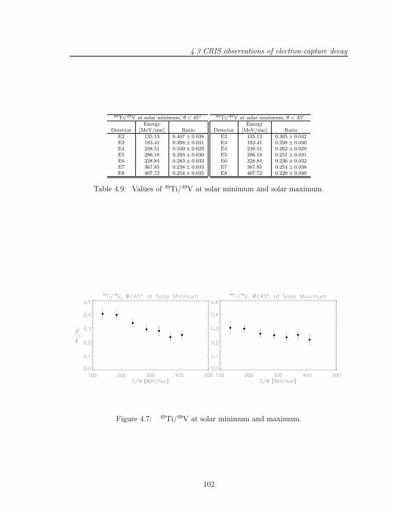
4.3 CRIS observations of electron-capture decay
49Ti/49V at solar minimum, θ < 45
EnergyDetector [MeV/nuc] Ratio
E2 135.13 0.407 ± 0.038E3 183.41 0.398 ± 0.031E4 238.51 0.340 ± 0.029E5 286.18 0.293 ± 0.030E6 328.84 0.283 ± 0.033E7 367.85 0.238 ± 0.033E8 407.72 0.254 ± 0.035
49Ti/49V at solar maximum, θ < 45
EnergyDetector [MeV/nuc] Ratio
E2 135.13 0.305 ± 0.042E3 183.41 0.298 ± 0.030E4 238.51 0.262 ± 0.029E5 286.18 0.251 ± 0.031E6 328.84 0.236 ± 0.032E7 367.85 0.254 ± 0.038E8 407.72 0.220 ± 0.040
Table 4.9: Values of 49Ti/49V at solar minimum and solar maximum.
Figure 4.7: 49Ti/49V at solar minimum and maximum.
102
4.3 CRIS observations of electron-capture decay
4.3.5 51Cr → 51V
As with 41Ca, 51Cr is somewhat significantly less abundant than its next heaviest
neighbor, 52Cr (see Figure 3.25). Using the method of Yanasak et al. (2001), 52Cr
contributes approximately an additional 0.5% to the 51Cr abundance. This correction
is too small compared to all other corrections listed in Table 4.10 to be considered
for this study. As with the mass-49 reaction, I have increased the acceptance angle
to 45 for Cr and V.
Chromium-51 decays to 51V with a laboratory half-life of ∼ 27.7 days. As with
the mass-49 reaction, it can be seen in Figure 4.8 that the energy dependent feature
in the EC decay of 51Cr can be seen during solar minimum. The abundance ratio
increases by a factor of about 1.8 from the highest to lowest energies during solar
minimum, corresponding to a greater likelihood for electron attachment and decay at
lower energies, as expected.
The value of 51V/51Cr remains relatively constant at all energies during solar max-
imum. The value at solar maximum is similar to the value above 300 MeV/nucleon
during solar minimum, corresponding to a greater average energy loss during solar
maximum of about 100 to 200 MeV/nucleon, similar to that seen in the 49Ti/49V
abundance ratio.
103

4.3 CRIS observations of electron-capture decay
51 Cr at solar minimum, θ < 45Fit Spallation Range-Energy Adjusted
Detector Abundance Correction Adj. Factor AbundanceE2 825.13 ± 31.62 1.084 ± 0.033 0.924 833.52 ± 43.86E3 1448.71 ± 41.00 1.143 ± 0.034 0.933 1558.04 ± 71.41E4 1067.24 ± 34.91 1.226 ± 0.037 0.941 1242.24 ± 60.48E5 785.16 ± 30.18 1.315 ± 0.039 0.947 986.33 ± 51.98E6 595.61 ± 26.32 1.407 ± 0.042 0.952 805.10 ± 45.91E7 484.69 ± 23.41 1.505 ± 0.045 0.956 703.57 ± 42.41E8 431.86 ± 22.98 1.614 ± 0.048 0.959 674.72 ± 43.37
51 Cr at solar maximum, θ < 45Fit Spallation Range-Energy Adjusted
Detector Abundance Correction Adj. Factor AbundanceE2 469.35 ± 23.70 1.084 ± 0.033 0.891 457.56 ± 28.39E3 917.43 ± 32.88 1.143 ± 0.034 0.912 964.78 ± 49.04E4 751.82 ± 29.05 1.226 ± 0.037 0.931 865.33 ± 45.73E5 610.28 ± 26.55 1.315 ± 0.039 0.944 764.44 ± 43.19E6 498.91 ± 24.02 1.407 ± 0.042 0.955 676.92 ± 40.72E7 370.80 ± 20.25 1.505 ± 0.045 0.965 543.23 ± 35.54E8 278.41 ± 18.02 1.614 ± 0.048 0.973 441.10 ± 32.68
————————————————————————51 Ti at solar minimum, θ < 45
Fit Spallation Range-Energy AdjustedDetector Abundance Correction Adj. Factor Abundance
E2 403.98 ± 21.25 1.084 ± 0.033 1.000 441.79 ± 28.17E3 599.53 ± 26.03 1.143 ± 0.034 1.000 691.22 ± 39.01E4 389.43 ± 21.05 1.226 ± 0.037 1.000 481.70 ± 31.30E5 305.00 ± 18.43 1.315 ± 0.039 1.000 404.56 ± 28.47E6 200.32 ± 15.24 1.407 ± 0.042 1.000 284.47 ± 23.95E7 124.76 ± 11.87 1.505 ± 0.045 1.000 189.47 ± 19.27E8 125.20 ± 11.51 1.614 ± 0.048 1.000 203.91 ± 20.13
51 Ti at solar maximum, θ < 45Fit Spallation Range-Energy Adjusted
Detector Abundance Correction Adj. Factor AbundanceE2 196.82 ± 15.08 1.084 ± 0.033 1.000 215.24 ± 18.23E3 308.20 ± 18.78 1.143 ± 0.034 1.000 355.33 ± 25.16E4 230.92 ± 15.81 1.226 ± 0.037 1.000 285.63 ± 22.11E5 184.60 ± 14.35 1.315 ± 0.039 1.000 244.86 ± 20.99E6 139.16 ± 12.33 1.407 ± 0.042 1.000 197.61 ± 18.90E7 103.37 ± 10.71 1.505 ± 0.045 1.000 156.98 ± 17.22E8 95.63 ± 10.12 1.614 ± 0.048 1.000 155.75 ± 17.41
Table 4.10: Measurements and corrections to the abundances of 51Cr and 51V dur-ing solar minimum and solar maximum. The spallation correction is found usingthe method discussed in §3.4. Chromium-51 has been spectrally adjusted to the51V energy range as discussed in Appendix B. The adjusted abundance includes anadditional SOFT efficiency correction factor of 1.009 ± 0.020 as discussed in §3.5.
104

4.3 CRIS observations of electron-capture decay
51V/51Cr at solar minimum, θ < 45
EnergyDetector [MeV/nuc] Ratio
E2 138.93 0.530 ± 0.044E3 188.69 0.444 ± 0.032E4 245.53 0.388 ± 0.031E5 294.76 0.410 ± 0.036E6 338.85 0.353 ± 0.036E7 379.20 0.269 ± 0.032E8 420.46 0.302 ± 0.036
51V/51Cr at solar maximum, θ < 45
EnergyDetector [MeV/nuc] Ratio
E2 138.93 0.470 ± 0.049E3 188.69 0.368 ± 0.032E4 245.53 0.330 ± 0.031E5 294.76 0.320 ± 0.033E6 338.85 0.292 ± 0.033E7 379.20 0.289 ± 0.037E8 420.46 0.353 ± 0.047
Table 4.11: Values of 51V/51Cr at solar minimum and solar maximum.
Figure 4.8: 51V/51Cr at solar minimum and maximum.
105

4.3 CRIS observations of electron-capture decay
4.3.6 53Mn → 53Cr
As with the EC decay of 41Ca, with a half-life of ∼ 106 years, 53Mn decays on a time
scale comparable to the other processes shown in Figure 4.1. Since the time scale
for EC decay is longer than that for electron stripping, we can assume that 53Mn
is effectively stable in the GCRs and that the production of 53Cr is dominated by
spallation from 56Fe and other heavier isotopes.
Table 4.12 lists the abundances and corrections to the isotopes in the mass-53
reaction. Table 4.13 and Figure 4.9 present the values of 53Cr/53Mn at solar min-
imum and solar maximum. It is difficult to determine whether the slow upturn in
53Cr/53Mn seen at low energies during solar minimum is a real effect or simply due to
statistical fluctuations. It is most likely, therefore, that the abundance ratio remains
essentially the same during solar minimum and solar maximum. As expected, there
is no immediate evidence of EC decay visible from this abundance ratio.
106

4.3 CRIS observations of electron-capture decay
53 Mn at solar minimum, θ < 30Fit Spallation Range-Energy Adjusted
Detector Abundance Correction Adj. Factor AbundanceE2 595.17 ± 24.88 1.080 ± 0.032 0.921 597.48 ± 32.99E3 1024.88 ± 32.61 1.137 ± 0.034 0.937 1101.60 ± 52.98E4 787.52 ± 28.47 1.218 ± 0.037 0.952 921.11 ± 47.03E5 618.91 ± 25.36 1.305 ± 0.039 0.962 784.47 ± 42.81E6 475.04 ± 22.11 1.398 ± 0.042 0.971 650.72 ± 38.31E7 375.37 ± 19.61 1.496 ± 0.045 0.978 554.41 ± 35.19E8 283.60 ± 17.03 1.606 ± 0.048 0.984 452.31 ± 31.68
53 Mn at solar maximum, θ < 30Fit Spallation Range-Energy Adjusted
Detector Abundance Correction Adj. Factor AbundanceE2 348.66 ± 18.89 1.080 ± 0.032 0.924 350.93 ± 22.84E3 573.06 ± 24.52 1.137 ± 0.034 0.930 611.40 ± 34.21E4 502.13 ± 22.75 1.218 ± 0.037 0.936 577.66 ± 33.45E5 421.39 ± 20.83 1.305 ± 0.039 0.940 521.86 ± 31.93E6 351.93 ± 18.88 1.398 ± 0.042 0.944 468.56 ± 30.29E7 279.18 ± 17.02 1.496 ± 0.045 0.947 399.05 ± 28.26E8 241.86 ± 15.91 1.606 ± 0.048 0.949 371.93 ± 27.89
————————————————————————53 Cr at solar minimum, θ < 30
Fit Spallation Range-Energy AdjustedDetector Abundance Correction Adj. Factor Abundance
E2 158.39 ± 13.48 1.080 ± 0.032 1.000 172.62 ± 15.95E3 258.00 ± 17.18 1.137 ± 0.034 1.000 295.98 ± 22.42E4 187.65 ± 14.91 1.218 ± 0.037 1.000 230.66 ± 20.13E5 144.47 ± 13.11 1.305 ± 0.039 1.000 190.29 ± 18.58E6 106.53 ± 11.02 1.398 ± 0.042 1.000 150.30 ± 16.46E7 85.71 ± 10.01 1.496 ± 0.045 1.000 129.43 ± 15.82E8 66.86 ± 8.80 1.606 ± 0.048 1.000 108.34 ± 14.78
53 Cr at solar maximum, θ < 30Fit Spallation Range-Energy Adjusted
Detector Abundance Correction Adj. Factor AbundanceE2 107.63 ± 11.08 1.080 ± 0.032 1.000 117.31 ± 12.79E3 152.14 ± 13.51 1.137 ± 0.034 1.000 174.54 ± 16.73E4 156.42 ± 13.16 1.218 ± 0.037 1.000 192.28 ± 17.60E5 107.48 ± 11.04 1.305 ± 0.039 1.000 141.57 ± 15.42E6 80.32 ± 9.59 1.398 ± 0.042 1.000 113.31 ± 14.13E7 83.08 ± 9.56 1.496 ± 0.045 1.000 125.46 ± 15.12E8 68.07 ± 8.88 1.606 ± 0.048 1.000 110.28 ± 14.92
Table 4.12: Measurements and corrections to the abundances of 53Mn and 53Cr duringsolar minimum and solar maximum. The spallation correction is found using themethod discussed in §3.4. Mnlcium-53 has been spectrally adjusted to the 53Cr energyrange as discussed in Appendix B. The adjusted abundance includes an additionalSOFT efficiency correction factor of 1.009 ± 0.020 as discussed in §3.5.
107

4.3 CRIS observations of electron-capture decay
53Cr/53Mn at solar minimum, θ < 30
EnergyDetector [MeV/nuc] Ratio
E2 138.45 0.289 ± 0.031E3 187.45 0.269 ± 0.024E4 244.04 0.250 ± 0.025E5 293.47 0.243 ± 0.027E6 338.46 0.231 ± 0.029E7 379.95 0.233 ± 0.032E8 420.80 0.240 ± 0.037
53Cr/53Mn at solar maximum, θ < 30
EnergyDetector [MeV/nuc] Ratio
E2 138.45 0.334 ± 0.042E3 187.45 0.285 ± 0.032E4 244.04 0.333 ± 0.036E5 293.47 0.271 ± 0.034E6 338.46 0.242 ± 0.034E7 379.95 0.314 ± 0.044E8 420.80 0.297 ± 0.046
Table 4.13: Values of 53Cr/53Mn at solar minimum and solar maximum.
Figure 4.9: 53Cr/53Mn at solar minimum and maximum.
108

4.3 CRIS observations of electron-capture decay
4.3.7 54Mn → 54Cr
Manganese-54 decays to 54Cr by EC decay with a laboratory half-life of 312.1 days.
As mentioned in Table 4.1, however, 54Mn also decays to 54Fe by β− emission with
a highly uncertain half-life of 105 to 107 years. With this lower limit on the β−-
decay process, we can assume that at lower energies where electron attachment and
decay happens more rapidly than β−-decay, 54Mn decays only by electron-capture.
At higher energies, however, we cannot assume that 54Mn is stable as we can in the
cases of other EC decay isotopes, since the energy-independent β−-decay process can
still occur well within the galactic confinement time of 15 Ma (Yanasak et al., 2001).
I have extended the angle of acceptance to 45 for this reaction since 54Mn is rela-
tively scarce in the GCRs. Additionally, I have included a correction for the 0.7+0.5−0.7%
enhancement in 54Mn from the neutron-stripping of 55Mn in the CRIS shielding ma-
terial, since it contributes ∼ 1.5% to the abundance of 54Mn (see Table 4.14).
During solar minimum, the abundance ratio of 54Cr/54Mn increases below ∼ 250
MeV/nucleon by ∼ 1.5 from its value at higher energies. This effect is as expected:
54Cr is enhanced due to the effects of EC decay of 54Mn at low energies. The ratio
is relatively constant during solar maximum and is similar to the value above ∼ 300
MeV/nucleon during solar minimum, corresponding to a greater average energy loss
during solar maximum by about 150 MeV/nucleon. In the end, however, due to the
uncertainty associated with the destruction of 54Mn through the β-decay channel, it
will be difficult to use the mass-54 reaction to probe directly the effects of EC decay.
109

4.3 CRIS observations of electron-capture decay
54 Mn at solar minimum, θ < 45Fit Corrected Spallation Range-Energy Adjusted
Detector Abundance Abundance* Correction Adj. Factor AbundanceE2 257.95 ± 20.46 262.18 ± 20.95 1.086 ± 0.033 0.935 268.66 ± 23.55E3 419.55 ± 26.11 426.22 ± 27.08 1.146 ± 0.034 0.941 464.24 ± 33.91E4 311.28 ± 20.78 315.72 ± 21.36 1.232 ± 0.037 0.947 371.84 ± 28.51E5 207.71 ± 19.31 211.52 ± 19.70 1.324 ± 0.040 0.952 268.86 ± 26.85E6 181.67 ± 15.98 184.37 ± 16.26 1.420 ± 0.043 0.955 252.23 ± 24.03E7 120.16 ± 12.70 122.12 ± 12.88 1.521 ± 0.046 0.958 179.51 ± 20.00E8 124.68 ± 12.37 125.77 ± 12.47 1.634 ± 0.049 0.960 199.15 ± 21.00
54 Mn at solar maximum, θ < 45Fit Corrected Spallation Range-Energy Adjusted
Detector Abundance Abundance* Correction Adj. Factor AbundanceE2 165.13 ± 15.51 167.61 ± 15.75 1.086 ± 0.033 0.905 166.20 ± 16.73E3 308.85 ± 21.45 312.91 ± 21.96 1.146 ± 0.034 0.925 334.99 ± 26.43E4 238.52 ± 18.04 241.92 ± 18.44 1.232 ± 0.037 0.944 283.90 ± 23.94E5 189.97 ± 16.21 192.43 ± 16.46 1.324 ± 0.040 0.958 246.19 ± 22.86E6 132.89 ± 12.83 134.91 ± 13.02 1.420 ± 0.043 0.969 187.26 ± 19.30E7 96.99 ± 13.21 98.71 ± 13.33 1.521 ± 0.046 0.978 148.20 ± 20.72E8 82.95 ± 11.37 84.23 ± 11.45 1.634 ± 0.049 0.986 137.01 ± 19.28
————————————————————————54 Cr at solar minimum, θ < 45
Fit Spallation Range-Energy AdjustedDetector Abundance Correction Adj. Factor Abundance
E2 155.34 ± 13.39 1.086 ± 0.033 1.000 170.23 ± 15.90E3 226.83 ± 16.04 1.146 ± 0.034 1.000 262.41 ± 20.83E4 154.92 ± 13.06 1.232 ± 0.037 1.000 192.60 ± 17.66E5 96.61 ± 10.45 1.324 ± 0.040 1.000 129.04 ± 14.72E6 77.97 ± 9.43 1.420 ± 0.043 1.000 111.70 ± 14.09E7 47.82 ± 7.14 1.521 ± 0.046 1.000 73.39 ± 11.27E8 55.31 ± 8.15 1.634 ± 0.049 1.000 91.20 ± 13.84
54 Cr at solar maximum, θ < 45Fit Spallation Range-Energy Adjusted
Detector Abundance Correction Adj. Factor AbundanceE2 68.38 ± 8.99 1.086 ± 0.033 1.000 74.94 ± 10.22E3 136.91 ± 12.62 1.146 ± 0.034 1.000 158.38 ± 15.68E4 78.88 ± 9.26 1.232 ± 0.037 1.000 98.07 ± 12.04E5 82.30 ± 9.60 1.324 ± 0.040 1.000 109.93 ± 13.42E6 56.27 ± 7.92 1.420 ± 0.043 1.000 80.61 ± 11.71E7 39.11 ± 7.29 1.521 ± 0.046 1.000 60.02 ± 11.40E8 35.92 ± 6.34 1.634 ± 0.049 1.000 59.22 ± 10.67
Table 4.14: Measurements and corrections to the abundances of 54Mn and 54Crduring solar minimum and solar maximum. The spallation correction is found usingthe method discussed in §3.4. Manganese-54 has been spectrally adjusted to the54Cr energy range as discussed in Appendix B. The adjusted abundance includes anadditional SOFT efficiency correction factor of 1.009 ± 0.020 as discussed in §3.5.*Corrected abundance includes the effects of neutron-stripping of 55Mn in the CRISshielding material.
110
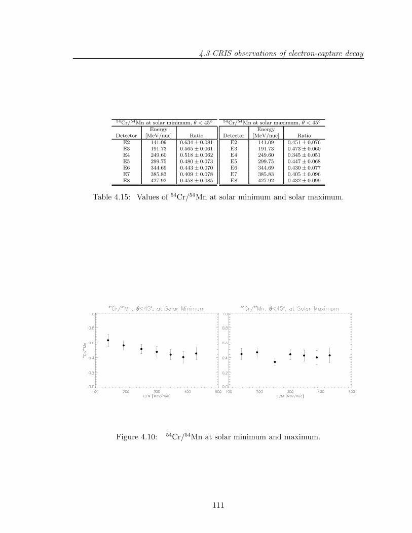
4.3 CRIS observations of electron-capture decay
54Cr/54Mn at solar minimum, θ < 45
EnergyDetector [MeV/nuc] Ratio
E2 141.09 0.634 ± 0.081E3 191.73 0.565 ± 0.061E4 249.60 0.518 ± 0.062E5 299.75 0.480 ± 0.073E6 344.69 0.443 ± 0.070E7 385.83 0.409 ± 0.078E8 427.92 0.458 ± 0.085
54Cr/54Mn at solar maximum, θ < 45
EnergyDetector [MeV/nuc] Ratio
E2 141.09 0.451 ± 0.076E3 191.73 0.473 ± 0.060E4 249.60 0.345 ± 0.051E5 299.75 0.447 ± 0.068E6 344.69 0.430 ± 0.077E7 385.83 0.405 ± 0.096E8 427.92 0.432 ± 0.099
Table 4.15: Values of 54Cr/54Mn at solar minimum and solar maximum.
Figure 4.10: 54Cr/54Mn at solar minimum and maximum.
111

4.3 CRIS observations of electron-capture decay
4.3.8 55Fe → 55Mn
Iron-55 decays to 55Mn with a half-life of just under 3 years. The 55Mn is an abundant
isotope of Mn and is well-resolved from the other two stable isotopes, 53Mn and 54Mn
(see Figure 3.26). The 55Fe isotope, on the other hand, is very difficult to resolve from
the extremely abundant 56Fe, as is apparent from Figure 3.27. Additionally, the effect
of neutron stripping from 56Fe in the shielding material above CRIS may enhance the
abundance of 55Fe observed at 1 AU by more than 10%. Using the method of Yanasak
et al. (2001), this correction has been taken into account for 55Fe. This correction
adds substantially to uncertainty in the 55Fe measurement (see Table 4.16).
Due to the difficulty involved in resolving 55Fe from 56Fe, I have restricted the
data to include only those events with zenith angle, θ < 25. Figure 4.11 shows the
Fe mass histograms in three detectors during periods of solar minimum and solar
maximum with θ < 25. Included in these plots are the same mass histograms with
the number of counts multiplied by 10 to show more detail.
The values for 55Mn/55Fe during solar minimum and maximum are listed in Table
4.17. It is immediately evident from Figure 4.12 that this daughter-to-parent abun-
dance ratio exhibits the characteristic upturn at low energies due to the decay of 55Fe
to 55Mn. The abundance ratio at solar maximum, however, agrees with the solar
minimum abundance ratio at all energies within the error bars on the data points at
solar maximum. It is therefore difficult to make a qualitative argument for energy
loss from the EC decay of 55Fe.
112

4.3 CRIS observations of electron-capture decay
55 Fe at solar minimum, θ < 25Fit Corrected Spallation Range-Energy Adjusted
Detector Abundance Abundance* Correction Adj. Factor AbundanceE2 440.81 ± 24.75 494.16 ± 47.36 1.080 ± 0.032 0.920 495.55 ± 50.74E3 850.20 ± 34.40 941.38 ± 77.56 1.137 ± 0.034 0.932 1005.97 ± 90.47E4 658.62 ± 29.40 728.77 ± 61.06 1.218 ± 0.037 0.942 844.01 ± 76.98E5 563.39 ± 27.40 617.04 ± 49.51 1.306 ± 0.039 0.950 772.11 ± 67.93E6 476.29 ± 24.64 520.26 ± 41.89 1.399 ± 0.042 0.956 702.19 ± 61.95E7 391.96 ± 21.61 425.20 ± 33.64 1.498 ± 0.045 0.961 617.81 ± 53.72E8 318.21 ± 20.49 348.42 ± 30.98 1.608 ± 0.048 0.966 545.84 ± 52.37
55 Fe at solar maximum, θ < 25Fit Corrected Spallation Range-Energy Adjusted
Detector Abundance Abundance* Correction Adj. Factor AbundanceE2 308.16 ± 20.76 337.66 ± 30.74 1.080 ± 0.032 0.926 340.74 ± 33.36E3 520.79 ± 27.09 577.01 ± 50.70 1.137 ± 0.034 0.931 616.02 ± 58.50E4 487.14 ± 24.94 535.05 ± 44.41 1.218 ± 0.037 0.935 615.01 ± 55.65E5 407.68 ± 23.02 447.52 ± 38.27 1.306 ± 0.039 0.938 553.16 ± 51.34E6 319.98 ± 20.47 355.01 ± 33.63 1.399 ± 0.042 0.941 471.53 ± 47.79E7 294.18 ± 19.24 322.37 ± 28.97 1.498 ± 0.045 0.943 459.53 ± 44.50E8 265.33 ± 18.24 290.60 ± 26.65 1.608 ± 0.048 0.945 445.43 ± 43.89
————————————————————————55 Mn at solar minimum, θ < 25
Fit Spallation Range-Energy AdjustedDetector Abundance Correction Adj. Factor Abundance
E2 360.64 ± 19.27 1.080 ± 0.032 1.000 393.01 ± 25.33E3 587.30 ± 24.77 1.137 ± 0.034 1.000 673.68 ± 37.38E4 444.19 ± 21.30 1.218 ± 0.037 1.000 546.03 ± 32.76E5 347.47 ± 19.04 1.306 ± 0.039 1.000 457.76 ± 30.03E6 307.63 ± 17.73 1.399 ± 0.042 1.000 434.31 ± 29.52E7 243.43 ± 15.86 1.498 ± 0.045 1.000 368.01 ± 27.40E8 185.31 ± 13.82 1.608 ± 0.048 1.000 300.66 ± 24.90
55 Mn at solar maximum, θ < 25Fit Spallation Range-Energy Adjusted
Detector Abundance Correction Adj. Factor AbundanceE2 220.48 ± 15.07 1.080 ± 0.032 1.000 240.27 ± 18.56E3 371.33 ± 19.61 1.137 ± 0.034 1.000 425.94 ± 27.24E4 341.60 ± 18.64 1.218 ± 0.037 1.000 419.91 ± 27.47E5 278.95 ± 16.87 1.306 ± 0.039 1.000 367.49 ± 25.88E6 220.53 ± 14.95 1.399 ± 0.042 1.000 311.34 ± 23.90E7 194.29 ± 14.41 1.498 ± 0.045 1.000 293.73 ± 24.22E8 181.43 ± 13.73 1.608 ± 0.048 1.000 294.36 ± 24.67
Table 4.16: Measurements and corrections to the abundances of 55Fe and 55Mnduring solar minimum and solar maximum. The spallation correction is found usingthe method discussed in §3.4. Iron-55 has been spectrally adjusted to the 55Mn energyrange as discussed in Appendix B. The adjusted abundance includes an additionalSOFT efficiency correction factor of 1.009 ± 0.020 as discussed in §3.5. *Correctedabundance includes the effects of neutron-stripping of 56Fe in the CRIS shieldingmaterial.
113

4.3 CRIS observations of electron-capture decay
Figure 4.11: Fe mass histograms at solar minimum (top row) and solar maximum(bottom row) for θ < 25. The three columns are data from detectors E3, E5 andE7. The superposed off-scale histograms show the numbers of counts × 10 for thepurposes of magnifying the 55Fe peak.
55Mn/55Fe at solar minimum, θ < 25
EnergyDetector [MeV/nuc] Ratio
E2 140.84 0.793 ± 0.096E3 190.55 0.670 ± 0.071E4 248.08 0.647 ± 0.071E5 298.40 0.593 ± 0.065E6 344.35 0.619 ± 0.069E7 386.77 0.596 ± 0.068E8 428.36 0.551 ± 0.070
55Mn/55Fe at solar maximum, θ < 25
EnergyDetector [MeV/nuc] Ratio
E2 140.84 0.705 ± 0.088E3 190.55 0.691 ± 0.079E4 248.08 0.683 ± 0.076E5 298.40 0.664 ± 0.077E6 344.35 0.660 ± 0.084E7 386.77 0.639 ± 0.081E8 428.36 0.661 ± 0.085
Table 4.17: Values of 55Mn/55Fe at solar minimum and solar maximum.
Figure 4.12: 55Mn/55Fe at solar minimum and maximum.
114
4.3 CRIS observations of electron-capture decay
4.3.9 57Co → 57Fe
Cobalt-57 decays to 57Fe with a half-life of 271.8 days. As can be seen from Figure
3.28, both stable isotopes of Co are extremely rare in the GCRs. Furthermore, 57Fe
shares the same problem with 55Fe in that it is very difficult to resolve from the
extremely abundant 56Fe (see Figure 4.11). There is therefore an inherent competi-
tion in the calculation of the daughter-to-parent abundance ratio for this reaction:
increased statistics are needed for 57Co, whereas decreasing statistics for 57Fe would
make it easier to resolve. Catering to both of these factors, I have used data with
θ < 30 for this study.
Table 4.18 lists the measurements and corrections to each abundance during pe-
riods of solar minimum and solar maximum. Note that the abundance of 57Co was
found by counting events since the 57Co and 59Co peaks are so well-resolved in the
data. Table 4.19 gives the values of 57Fe/57Co during solar minimum and solar max-
imum. The uncertainties on these measurements are large due to limited statistics
for the 57Co measurement and the large correlation between the uncertainties on the
56Fe and 57Fe fit abundances.
From the plots in Figure 4.13, it is evident that the error bars are too large to
make a sound case for evidence of energy loss. Additionally, as with the mass-44
reaction, the decay of the less-abundant 57Co increases the abundance of 57Fe by a
very small amount. The abundance ratios for this reaction give little insight into the
effects of solar modulation on EC decay isotopes.
115
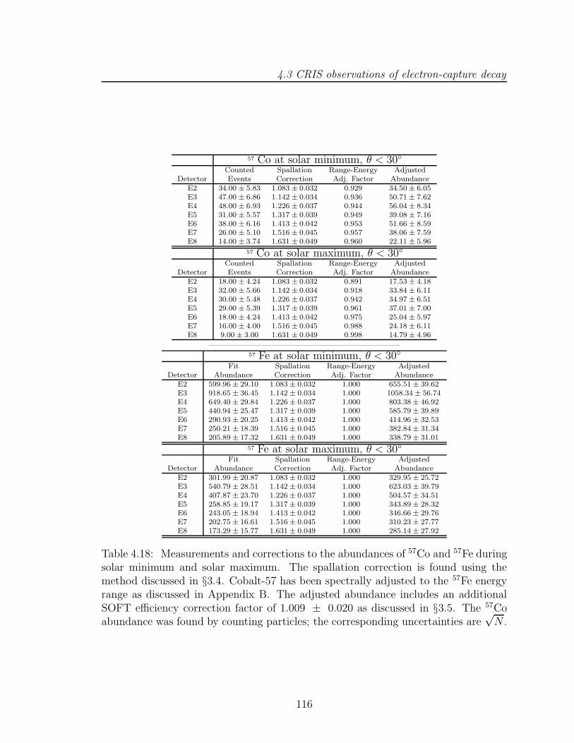
4.3 CRIS observations of electron-capture decay
57 Co at solar minimum, θ < 30Counted Spallation Range-Energy Adjusted
Detector Events Correction Adj. Factor AbundanceE2 34.00 ± 5.83 1.083 ± 0.032 0.929 34.50 ± 6.05E3 47.00 ± 6.86 1.142 ± 0.034 0.936 50.71 ± 7.62E4 48.00 ± 6.93 1.226 ± 0.037 0.944 56.04 ± 8.34E5 31.00 ± 5.57 1.317 ± 0.039 0.949 39.08 ± 7.16E6 38.00 ± 6.16 1.413 ± 0.042 0.953 51.66 ± 8.59E7 26.00 ± 5.10 1.516 ± 0.045 0.957 38.06 ± 7.59E8 14.00 ± 3.74 1.631 ± 0.049 0.960 22.11 ± 5.96
57 Co at solar maximum, θ < 30Counted Spallation Range-Energy Adjusted
Detector Events Correction Adj. Factor AbundanceE2 18.00 ± 4.24 1.083 ± 0.032 0.891 17.53 ± 4.18E3 32.00 ± 5.66 1.142 ± 0.034 0.918 33.84 ± 6.11E4 30.00 ± 5.48 1.226 ± 0.037 0.942 34.97 ± 6.51E5 29.00 ± 5.39 1.317 ± 0.039 0.961 37.01 ± 7.00E6 18.00 ± 4.24 1.413 ± 0.042 0.975 25.04 ± 5.97E7 16.00 ± 4.00 1.516 ± 0.045 0.988 24.18 ± 6.11E8 9.00 ± 3.00 1.631 ± 0.049 0.998 14.79 ± 4.96
————————————————————————57 Fe at solar minimum, θ < 30
Fit Spallation Range-Energy AdjustedDetector Abundance Correction Adj. Factor Abundance
E2 599.96 ± 29.10 1.083 ± 0.032 1.000 655.51 ± 39.62E3 918.65 ± 36.45 1.142 ± 0.034 1.000 1058.34 ± 56.74E4 649.40 ± 29.84 1.226 ± 0.037 1.000 803.38 ± 46.92E5 440.94 ± 25.47 1.317 ± 0.039 1.000 585.79 ± 39.89E6 290.93 ± 20.25 1.413 ± 0.042 1.000 414.96 ± 32.53E7 250.21 ± 18.39 1.516 ± 0.045 1.000 382.84 ± 31.34E8 205.89 ± 17.32 1.631 ± 0.049 1.000 338.79 ± 31.01
57 Fe at solar maximum, θ < 30Fit Spallation Range-Energy Adjusted
Detector Abundance Correction Adj. Factor AbundanceE2 301.99 ± 20.87 1.083 ± 0.032 1.000 329.95 ± 25.72E3 540.79 ± 28.51 1.142 ± 0.034 1.000 623.03 ± 39.79E4 407.87 ± 23.70 1.226 ± 0.037 1.000 504.57 ± 34.51E5 258.85 ± 19.17 1.317 ± 0.039 1.000 343.89 ± 28.32E6 243.05 ± 18.94 1.413 ± 0.042 1.000 346.66 ± 29.76E7 202.75 ± 16.61 1.516 ± 0.045 1.000 310.23 ± 27.77E8 173.29 ± 15.77 1.631 ± 0.049 1.000 285.14 ± 27.92
Table 4.18: Measurements and corrections to the abundances of 57Co and 57Fe duringsolar minimum and solar maximum. The spallation correction is found using themethod discussed in §3.4. Cobalt-57 has been spectrally adjusted to the 57Fe energyrange as discussed in Appendix B. The adjusted abundance includes an additionalSOFT efficiency correction factor of 1.009 ± 0.020 as discussed in §3.5. The 57Coabundance was found by counting particles; the corresponding uncertainties are
√N .
116

4.3 CRIS observations of electron-capture decay
57Fe/57Co at solar minimum, θ < 30
EnergyDetector [MeV/nuc] Ratio
E2 145.45 19.003 ± 3.523E3 197.17 20.871 ± 3.330E4 257.02 14.336 ± 2.291E5 309.39 14.988 ± 2.929E6 357.13 8.032 ± 1.476E7 401.22 10.059 ± 2.168E8 444.68 15.323 ± 4.364
57Fe/57Co at solar maximum, θ < 30
EnergyDetector [MeV/nuc] Ratio
E2 145.45 18.820 ± 4.721E3 197.17 18.410 ± 3.523E4 257.02 14.429 ± 2.861E5 309.39 9.293 ± 1.917E6 357.13 13.845 ± 3.509E7 401.22 12.831 ± 3.438E8 444.68 19.285 ± 6.736
Table 4.19: Values of 57Fe/57Co at solar minimum and solar maximum.
Figure 4.13: 57Fe/57Co at solar minimum and maximum.
117

4.4 Summary of observations
4.4 Summary of observations
It is evident from the preceding sections that observation of the effects of electron-
capture decay in the sub-Fe GCRs is difficult for a number of reasons. Since there are
such low statistics for most isotopes in this regime, it becomes difficult to resolve any
distinct energy-dependent features from the uncertainties on the daughter-to-parent
abundance ratios. While greater numbers of events can be attained by increasing the
angle of acceptance in the detector, the isotopic resolution we can achieve by fitting
the mass histograms to a Gaussian suffers as a result.
The two most promising cases for evidence of energy-loss in the heliosphere due
to EC decay are 49V and 51Cr. In both cases, the parent isotopes are slightly more
abundant than the daughter isotopes and so the effects of electron-capture decay are
easily visible. By increasing the acceptance angle to 45 for these isotopes, there are
ample statistics to probe the effects of electron-capture without sacrificing the mass
resolution.
During solar minimum, the value of 49Ti/49V increases from ∼ 0.25 at high energies
to ∼ 0.40 at lower energies, meaning that ∼ 10% of 49V has decayed. During the same
period 51V/51Cr increases from ∼ 0.30 to ∼ 0.52, indicating that ∼ 15% of 51Cr has
decayed. Provided that a similar percentage of 44Ti and 57Co decay due to electron
capture, the resulting enhancement in the more abundant 44Ca and 57Fe would be
almost invisible.
To a lesser extent, the EC decay of 54Mn may provide some qualitative information
118

4.4 Summary of observations
about EC decay. The effect of β−-decay on 54Mn, however, limits the usefulness of
this reaction.
The next chapter will give an overview of the leaky-box propagation model, includ-
ing a description of the version used by our collaboration. The EC decay daughter-to-
parent abundance ratios will be compared to the results of our leaky-box propagation
model, modulated to 1 AU using the Fisk model discussed in §1.2.4.
119

Chapter 5
Comparison of CRIS data with aLeaky-Box model
5.1 The Leaky-Box model
The leaky-box model (LBM) for the propagation of GCRs in the interstellar medium
was first described by Cowsik et al. (1967). This model assumes a uniform distri-
bution of sources inside some specified volume filled with an entirely homogeneous
medium. Particles are accelerated at these sources and are free to propagate uni-
formly and escape at a constant rate from the “galaxy” defined by this volume. The
cosmic rays are never reaccelerated during propagation.
The model in its original form was found to behave better than the popular
matter-slab approximation and could correctly fit the observed decrease in secondary-
to-primary abundance ratios at low energies. Particles of a given rigidity should be
expected to follow any number of trajectories due to scattering by magnetic fields.
The pathlengths should, therefore, be different for different species and for different
rigidities. Additionally, since the energy loss by ionization increases with decreasing
120

5.1 The Leaky-Box model
energy, at low energies, detectors sample mainly the population of nuclei that have
traversed small amounts of matter.
In the steady-state situation (where particles are injected and escaping at the
same rate), the amount of matter traversed X is found to be
1
X=
1
Λl
+1
Λint
+1
Λion
, (5.1)
where Λl and Λint are the mean pathlengths for leakage from the Galaxy and nuclear
interaction, and Λion is the pathlength for ionization energy loss. Since different
species of nuclei at a given rigidity may have the same Λl, while Λint and Λion may
depend on the nuclear charge and mass, it is evident that a constant pathlength for
all particles may not be the best approximation.
The code for the LBM used by the CRIS collaboration was written and maintained
by collaborator Mark Wiedenbeck of Caltech/JPL. It is based on the formalism of
Meneguzzi et al. (1971) for the steady-state leaky-box model, for which the transport
equation for a given species, i, is given by
∂Ni(E)
∂t= 0 = −Ni(E)
τe− Ni(E)
γτi+Qi(E)
+ ∂∂E
[bi(E)Ni(E)] − [σα i(E)nHe + σp i(E)nH ] viNi(E)
+∑
j
∫ ∞0Nj(E
′) [nHeσα j i(E,E′) + nHσp j i(E,E
′)] vjdE′, (5.2)
where Ni(E) is the cosmic ray number density at energy per nucleon E, with τe as the
mean escape time and τi as the decay lifetime for unstable nuclei with Lorentz factor
γ (this term goes to zero for stable isotopes). The source term, Qi(E) is set to be
constant in time and space and the term bi(E) is simply the ionization energy loss per
121

5.1 The Leaky-Box model
Figure 5.1: (Sc+Ti+V)/Fe at solar minimum, with Leaky-Box Model predictionsoverlaid.dashed curve: the unmodulated interstellar LBM value.solid curves: the LBM with solar modulation parameters, φ = 350, 400, and 500 MV,corresponding to what one would expect during solar minimum.dotted curves: the LBM modulated by φ = 800, 900, 1000, and 1100 MV, correspond-ing what one would expect during solar maximum.closed circles: CRIS data (this work).open circles: HEAO-3-C2 data (Engelmann et al., 1990).
unit time, −(
∂E∂t
)
i. The total destruction cross sections for species i with velocity, vi,
are defined as σp i(E) and σα i(E) on H and He atoms with densities nH and nHe. The
production cross sections for species i from spallation of all possible parent nuclei j of
density Nj, velocity vj, and energy E ′ are σp j i(E,E′) and σα j i(E,E
′) on H and He
targets, respectively. In this way, the transport equation provides for almost every
process that can affect a given nucleus during propagation in the ISM.
The following are the parameters used as the code stands today. The source term
122
5.1 The Leaky-Box model
for all species describes a power law in rigidity going as R−2.35; this was adapted to
lower energies based on the work of Engelmann et al. (1990). The pathlength for
escape from the Galaxy, Λe, was modified from Soutoul and Ptuskin (1999), and is
given in Wiedenbeck et al. (2001) as
Λe = 35 g cm−2 β(
βR
1.0 GV
)0.6+
(
βR
1.3 GV
)−2.0 . (5.3)
It has been shown that the coefficient of 35 g cm−2 agrees well for all secondary-to-
primary abundance ratios from B/C to (Sc+Ti+V)/Fe. Figure 5.1 shows the CRIS
and HEAO-3-C2 data with LBM predictions at varying levels solar modulation. Note,
in particular, that the LBM correctly describes the observed peak in this abundance
ratio between the CRIS and HEAO-3-C2 data.
The density of hydrogen atoms is taken to be 0.34 cm−3 from Yanasak et al.
(2001) with a corresponding helium density of 10% that of hydrogen. The total and
partial interaction cross sections for this LBM are taken from Webber, Kish and
Schrier (1990), Knott et al. (1997), Chen et al. (1997) and Webber et al. (1998a)
and (1998b), and further scaled to match the data using Silberberg et al. (1983). The
treatment of electron-capture decay is discussed in §4. The cross sections for electron
attachment is based on the first-order Born approximation as formalized by Crawford
(1979); electron stripping is based on the Bohr formula and corrections applied by
Wilson (1978).
This LBM has been used in several studies involving cosmic-ray studies in many
energy ranges. More information about this code for our particular model can be
123

5.2 Comparison with EC decay abundance ratios
found in Leske (1993), Davis et al. (2001), and George et al. (2005).
5.2 Comparison with EC decay abundance ratios
This section will compare the daughter-to-parent abundance ratios for the EC decay
reactions of the best candidates for direct evidence of energy loss in the heliosphere
(i.e. the short-lived, somewhat abundant, otherwise stable isotopes) to the modulated
LBM predictions (Wiedenbeck, 2004). By comparing these abundance ratios during
the period of solar minimum and solar maximum, it will be possible to parameterize
the amount of solar modulation that the GCRs experience during the two phases of
the solar cycle. These EC decay isotopes include 37Ar, 44Ti, 49V, 51Cr and 55Fe.
124

5.2 Comparison with EC decay abundance ratios
5.2.1 37Ar → 37Cl
Figure 5.2: 37Cl/37Ar at solar minimum, with Leaky-Box Model predictions overlaid.dashed curve: the unmodulated interstellar LBM value.solid curves: the LBM with solar modulation parameters, φ = 350, 400, and 500 MV,corresponding to what one would expect during solar minimum. The dashed curveonly deviates from the modulated curves below ∼ 100 MeV/nucleon, because only atthese energies can electron attachment compete with other losses.
As was discussed in §4.3.1, the daughter-to-parent abundance ratios for the EC
decay of 37Ar to 37Cl exhibit no distinct energy-dependent features from solar mini-
mum to solar maximum. This fact is demonstrated further by comparing 37Cl/37Ar
to a set of curves created by our leaky-box model modulated in the heliosphere using
different values of φ.
Figure 5.2 shows this abundance ratio during the period of solar minimum with
modulated LBM curves overlaid. It is evident that the model overpredicts the value
125
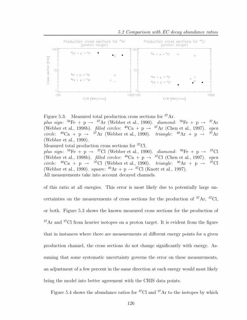
5.2 Comparison with EC decay abundance ratios
Figure 5.3: Measured total production cross sections for 37Ar.plus sign: 56Fe + p → 37Ar (Webber et al., 1990). diamond : 56Fe + p → 37Ar(Webber et al., 1998b). filled circles: 40Ca + p → 37Ar (Chen et al., 1997). opencircle: 40Ca + p → 37Ar (Webber et al., 1990). triangle: 40Ar + p → 37Ar(Webber et al., 1990).Measured total production cross sections for 37Cl.plus sign: 56Fe + p → 37Cl (Webber et al., 1990). diamond : 56Fe + p → 37Cl(Webber et al., 1998b). filled circles: 40Ca + p → 37Cl (Chen et al., 1997). opencircle: 40Ca + p → 37Cl (Webber et al., 1990). triangle: 40Ar + p → 37Cl(Webber et al., 1990). square: 40Ar + p → 37Cl (Knott et al., 1997).All measurements take into account decayed channels.
of this ratio at all energies. This error is most likely due to potentially large un-
certainties on the measurements of cross sections for the production of 37Ar, 37Cl,
or both. Figure 5.3 shows the known measured cross sections for the production of
37Ar and 37Cl from heavier isotopes on a proton target. It is evident from the figure
that in instances where there are measurements at different energy points for a given
production channel, the cross sections do not change significantly with energy. As-
suming that some systematic uncertainty governs the error on these measurements,
an adjustment of a few percent in the same direction at each energy would most likely
bring the model into better agreement with the CRIS data points.
Figure 5.4 shows the abundance ratios for 37Cl and 37Ar to the isotopes by which
126

5.2 Comparison with EC decay abundance ratios
Figure 5.4: Abundance ratios of 37Cl/40Ca and 37Ar/40Ar with Leaky-Box Modelpredictions.dashed curve: the unmodulated interstellar LBM value.solid curves: the LBM with solar modulation parameters φ = 350, 400, and 500 MV,corresponding to what one would expect during solar minimum.
the majority of each are created by spallation. Even though 40Ar is a little less than
half as abundant as 40Ca in the CRIS data, the cross section for production of 37Ar
by 40Ar is a factor of 10 to 15 higher than that for 40Ca. In addition, despite the
relatively small cross sections for production of 37Ar and 37Cl by 56Fe, this isotope is
so abundant (more than 10 times that of 40Ca and more than 200 times that of 40Ar)
that it is a significant contributor to the abundances of the mass-37 isotopes. It is
evident from Figure 5.4 that the model underproduces 37Ar by spallation of 40Ar and
127

5.2 Comparison with EC decay abundance ratios
56Fe and overproduces 37Cl by spallation of 40Ca and 56Fe. Better measurements of
these cross sections would result in better fits to our LBM.
Nevertheless, even with better cross section data, the mass-37 reaction gives little
information about energy loss in the heliosphere. The feature in 37Cl/37Ar below
∼ 150 MeV/nucleon in the unmodulated LBM model in Figure 5.2 (dashed curve)
is all but erased after modulation in the heliosphere (solid curve): distinguishing
between different values of φ is very difficult.
128

5.2 Comparison with EC decay abundance ratios
5.2.2 44Ti → 44Ca
Figure 5.5: 44Ca/44Ti at solar minimum, with Leaky-Box Model predictions overlaid.dashed curve: the unmodulated interstellar LBM value.solid curves: the LBM with solar modulation parameters, φ = 350, 400, and 500 MV,corresponding to what one would expect during solar minimum.
The decay of 44Ti to 44Ca is also a very difficult reaction to study due mainly
to the extremely low statistics for 44Ti. As with the mass-37 reaction, the LBM
overestimates the value of 44Ca/44Ti, due most likely to inaccurate cross section mea-
surements for 44Ti and 44Ca. Figure 5.6 shows a plot of the known measurements for
production of 44Ti and 44Ca implemented in our LBM. As expected, the cross sections
for production of 44Ti by spallation of 56Fe on hydrogen are extremely small.
Figure 5.7 shows the abundance ratios of 44Ti and 44Ca to 56Fe. From the figure,
we can see that the LBM produces approximately the correct amount of 44Ca, while
129

5.2 Comparison with EC decay abundance ratios
Figure 5.6: Measured total production cross sections for 44Ti.open circle: 56Fe + p → 44Ti (Webber et al., 1990). diamond : 56Fe + p → 44Ti(Webber et al., 1998b). Measured total production cross sections for 44Ca.open circle: 56Fe + p → 44Ca (Webber et al., 1990). diamond : 56Fe + p → 44Ca(Webber et al., 1998b).All measurements take into account decayed channels.
it seems to be underproducing 44Ti by as much as a factor of 1.5 or 2. This under-
production of 44Ti is as expected in Figure 5.5: the daughter-to-parent ratio is about
2 times higher in the LBM than in the CRIS data. As before, however, a correction
to the LBM of the cross section for production of 44Ti by 56Fe would still make it
impossible to distinguish between the modulated values at solar minimum.
130

5.2 Comparison with EC decay abundance ratios
Figure 5.7: Abundance ratios of 44Ti/56Fe and 44Ca/56Fe with Leaky-Box Modelpredictions.dashed curve: the unmodulated interstellar LBM value.solid curves: the LBM with solar modulation parameters φ = 350, 400, and 500 MV,corresponding to what one would expect during solar minimum.
131

5.2 Comparison with EC decay abundance ratios
5.2.3 49V → 49Ti
As discussed in §4.3.4, qualitatively, the decay of 49V to 49Ti exhibits a distinct energy
dependence during solar minimum: the value of 49Ti/49V increases significantly at low
energies owing to the higher cross section for electron attachment for 49V. During solar
maximum, the value of 49Ti/49V is essentially independent of energy.
Unlike with 37Ar, 37Cl, 44Ti and 44Ca, there have been a few more experiments
conducted to measure the production cross sections for 49V and 49Ti. Figure 5.8 shows
the available cross section data for both 49V and 49Ti. In the case of 49V, despite the
fact that 50Cr, 52Cr and 55Mn have the highest cross sections, 56Fe is more than 20
times more abundant than 55Mn and 50Cr and more than 10 times more than 52Cr.
Iron-56 is, as well, the greatest contributor to the abundance of 49V by similar factors
over 50Cr, 52Cr and 55Mn.
Figure 5.9 shows the abundance ratios of 49V to 50Cr, 52Cr, 55Mn, 54Fe and 56Fe.
With the exception of 49V/50Cr (and perhaps 49V/54Fe), the LBM is in good agree-
ment with the CRIS data in all cases. Since 50Cr and 54Fe most likely contribute
little to the abundance of 49V, adjustments to these production cross sections will not
change significantly the LBM results for the intensity of 49V.
The abundance ratios of isotopes for which 49Ti production cross sections are
known are plotted in Figure 5.10. As with 49V, 56Fe contributes most to the produc-
tion of 49Ti (almost 10 times as much as 52Cr and more than 30 times more than
55Mn). Figure 5.10 shows the abundance ratios 49Ti/52Cr, 49Ti/55Mn and 49Ti/56Fe.
132

5.2 Comparison with EC decay abundance ratios
Figure 5.8: Measured total production cross sections for 49V.plus sign: 56Fe + p → 49V (Webber et al., 1990). diamond : 56Fe + p → 49V(Webber et al., 1998b). filled circles: 54Fe + p → 49V (Webber et al., 1998c). opencircle: 55Mn + p → 49V (Webber et al., 1998c). triangle: 52Cr + p → 49V(Webber et al., 1998c). square: 50Cr + p → 49V (Webber et al., 1998c).Measured total production cross sections for 49Ti.plus sign: 56Fe + p → 49Ti (Webber et al., 1990). diamond : 56Fe + p → 49Ti(Webber et al., 1998b). open circle: 55Mn + p → 49Ti (Webber et al., 1998c). tri-angle: 52Cr + p → 49Ti (Webber et al., 1998c).All measurements take into account decayed channels.
We can see that the LBM slightly overestimates 49Ti/52Cr, but agrees rather well
with the data for 49Ti/55Mn. In Figure 5.10(c), the LBM agrees well with the data
for 49Ti/56Fe in detectors E2, E3, and E4, but is too high at higher energies. Figure
5.10(d) shows the same data with the LBM predictions where the production cross
section for all channels to 49Ti have been decreased by 15%. Assuming, reasonably,
that the uncertainties for measuring these production cross sections may be as high
as around 20%, we see no problem with such an adjustment. It is evident from (d)
that the LBM is in better agreement with the data at all energies when this cross
section adjustment is included.
The results for the LBM prediction for 49Ti/49V with this 15% adjustment to
133

5.2 Comparison with EC decay abundance ratios
Figure 5.9: Abundance ratios 49V/50Cr, 49V/52Cr, 49V/55Mn, 49V/54Fe and 49V/56Fewith Leaky-Box Model predictions.dashed curve: the unmodulated interstellar LBM value.solid curves: the LBM with solar modulation parameters φ = 350, 400, and 500 MV,corresponding to what one would expect during solar minimum.
the production cross sections for 49Ti are presented in Figure 5.11. We can see
from the figure, that our modulated LBM agrees very well with the measured value
of 49Ti/49V at all energies during both solar minimum and solar maximum. The
model verifies what we expect. Events observed during solar maximum are from a
population of GCRs that were propagating at higher energies than the population
from which events are observed during solar minimum: particles lose more energy in
the heliosphere during solar maximum than during solar minimum.
134

5.2 Comparison with EC decay abundance ratios
Figure 5.10: Abundance ratios 49Ti/52Cr, 49Ti/55Mn and 49Ti/56Fe with Leaky-BoxModel predictions.dashed curve: the unmodulated interstellar LBM value.solid curves: the LBM with solar modulation parameters φ = 350, 400, and 500 MV,corresponding to what one would expect during solar minimum.(c): 49Ti/56Fe using the nominal cross section values from Figure 5.8. (d): 49Ti/56Fewhere the production cross section by 56Fe has been decreased by 15%.
135
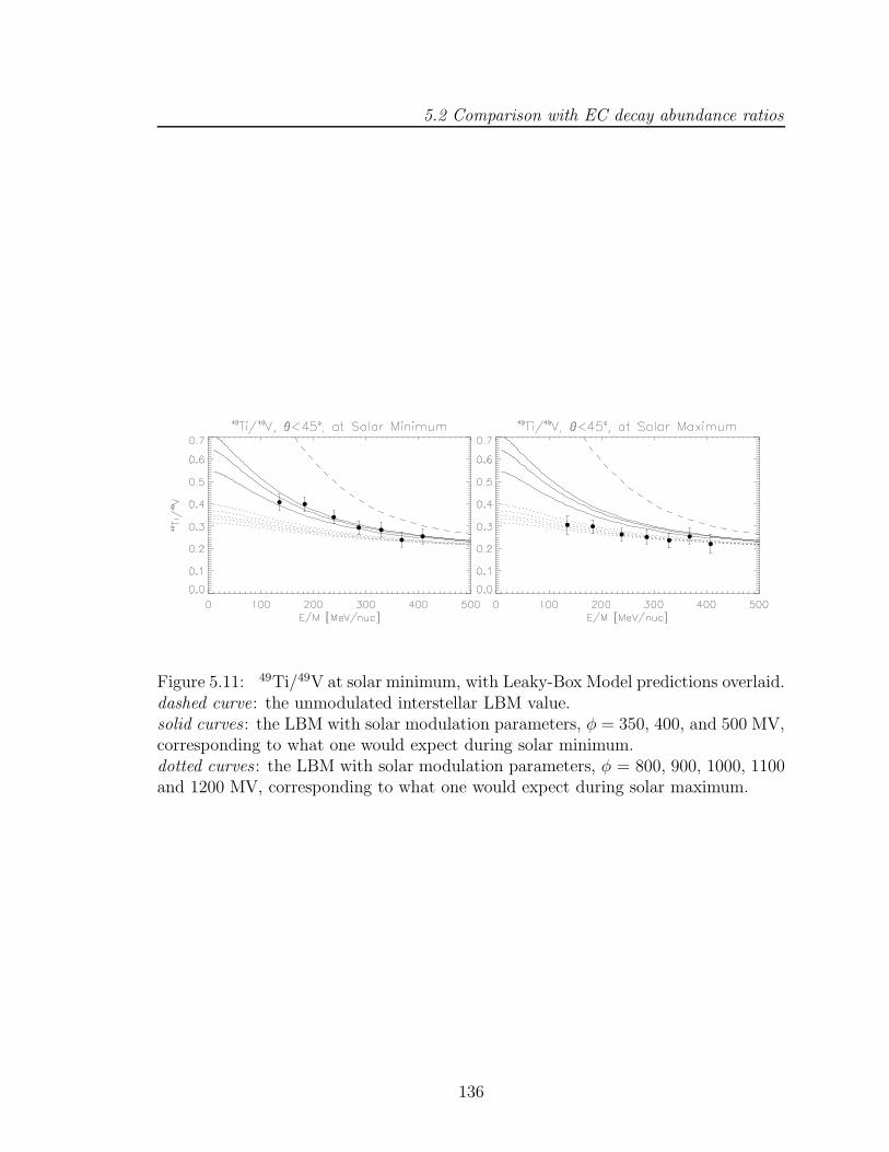
5.2 Comparison with EC decay abundance ratios
Figure 5.11: 49Ti/49V at solar minimum, with Leaky-Box Model predictions overlaid.dashed curve: the unmodulated interstellar LBM value.solid curves: the LBM with solar modulation parameters, φ = 350, 400, and 500 MV,corresponding to what one would expect during solar minimum.dotted curves: the LBM with solar modulation parameters, φ = 800, 900, 1000, 1100and 1200 MV, corresponding to what one would expect during solar maximum.
136
5.2 Comparison with EC decay abundance ratios
5.2.4 51Cr → 51V
As with the decay of 49V, the ratio 51V/51Cr exhibits distinct energy dependence at
solar minimum (Figure 4.8). The value of 51V/51Cr is also relatively indepedent of
energy during solar maximum, as it is with 49Ti/49V.
Figure 5.12 gives the known measurements for production cross sections for 51Cr
and 51V. Understandably, the largest cross section for the production of 51Cr comes
from stripping a neutron from the more abundant 52Cr. As we have seen in the
previous sections, however, the spallation of 56Fe accounts for the majority of GCR
51Cr. In this case, it contributes more than 5 times more to the abundance of 51Cr
than 54Fe, 55Mn and 52Cr combined. In the case of 51V, however, 56Fe is only about
2.5 times more significant than 52Cr in the production of 51V, while it is more than
10 times more significant than production by 55Mn.
The abundance ratios plotted in Figure 5.13 show 51Cr versus its four main gen-
erators by spallation in the ISM. On the whole, the LBM predictions are in good
agreement with the data, with the most important ratio, 51Cr/56Fe overestimated by
the LBM by only a few percent.
Figure 5.14 shows similar plots for 51V. The ratios 51V/52Cr and 51V/56Fe corre-
spond to the most significant channels for 51V production. While the LBM in both
cases agrees somewhat well with the CRIS data, the model is high by a few percent at
all energies for all three abundance ratios (including 51V/56Fe). The underestimation
of 51V as possible evidence for reacceleration will be discussed in §6.
137

5.2 Comparison with EC decay abundance ratios
Figure 5.12: Measured total production cross sections for 51Cr.plus sign: 56Fe + p → 51Cr (Webber et al., 1990). diamond : 56Fe + p → 51Cr(Webber et al., 1998b). filled circles: 54Fe + p → 51Cr (Webber et al., 1998c). opencircle: 55Mn + p → 51Cr (Webber et al., 1998c). triangle: 52Cr + p → 51Cr(Webber et al., 1998c).Measured total production cross sections for 51V.plus sign: 56Fe + p → 51V (Webber et al., 1990). diamond : 56Fe + p → 51V(Webber et al., 1998b). open circle: 55Mn + p → 51V (Webber et al., 1998c). trian-gle: 52Cr + p → 51V (Webber et al., 1998c).All measurements take into account decayed channels.
The LBM predictions for the daughter-to-parent abundance ratio for the EC decay
of 51Cr are presented in Figure 5.15. As in the case of the mass-49 ratios presented
in Figure 5.11, the LBM for 51V/51Cr agrees well with the data during both solar
minimum and solar maximum.
138

5.2 Comparison with EC decay abundance ratios
Figure 5.13: Abundance ratios 51Cr/52Cr, 51Cr/55Mn, 51Cr/54Fe and 51Cr/56Fe withLeaky-Box Model predictions.dashed curve: the unmodulated interstellar LBM value.solid curves: the LBM with solar modulation parameters φ = 350, 400, and 500 MV,corresponding to what one would expect during solar minimum.
139

5.2 Comparison with EC decay abundance ratios
Figure 5.14: Abundance ratios 51V/52Cr, 51V/55Mn and 51V/56Fe with Leaky-BoxModel predictions.dashed curve: the unmodulated interstellar LBM value.solid curves: the LBM with solar modulation parameters φ = 350, 400, and 500 MV,corresponding to what one would expect during solar minimum.
140
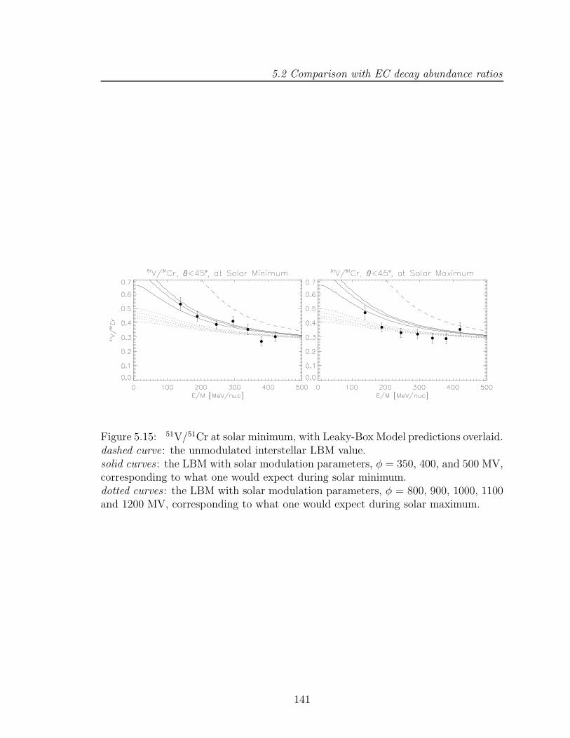
5.2 Comparison with EC decay abundance ratios
Figure 5.15: 51V/51Cr at solar minimum, with Leaky-Box Model predictions overlaid.dashed curve: the unmodulated interstellar LBM value.solid curves: the LBM with solar modulation parameters, φ = 350, 400, and 500 MV,corresponding to what one would expect during solar minimum.dotted curves: the LBM with solar modulation parameters, φ = 800, 900, 1000, 1100and 1200 MV, corresponding to what one would expect during solar maximum.
141

5.2 Comparison with EC decay abundance ratios
5.2.5 55Fe → 55Mn
Figure 5.16: 55Mn/55Fe at solar minimum, with Leaky-Box Model predictions over-laid.dashed curve: the unmodulated interstellar LBM value.solid curves: the LBM with solar modulation parameters, φ = 350, 400, and 500 MV,corresponding to what one would expect during solar minimum.dotted curves: the LBM with solar modulation parameters, φ = 800, 900, 1000, 1100and 1200 MV, corresponding to what one would expect during solar maximum.
Figure 5.16 presents the daughter-to-parent abundance ratios for the EC decay of
55Fe with our LBM predictions. It is evident from both plots that the solar minimum
and solar maximum data have the same shape as their respective LBM curves, but
that the curves overpredict what the data show by around a factor of 2 in each case.
The predominant channel by which both 55Fe and 55Mn are created in the ISM
is, as usual, by spallation of 56Fe. Figure 5.17 shows the experimental cross sections
for production of these isotopes. The ratios of the mass-55 isotopes to their largest
contributors by spallation are given in Figure 5.18. The results are as one might
expect: the LBM is in excellent agreement with the data for 55Mn/56Fe, while it is
not in the cases of 55Fe/56Fe and 55Fe/58Ni. As shown in greater detail in Figure 4.11,
142

5.2 Comparison with EC decay abundance ratios
Figure 5.17: Measured total production cross sections for 55Fe.plus sign: 58Ni + p → 55Fe (Webber et al., 1990). triangle: 56Fe + p → 55Fe(Webber et al., 1990). diamond : 56Fe + p → 55Fe (Webber et al., 1998b). opencircle: 56Fe + p → 55Fe (Webber et al., 1998c).Measured total production cross sections for 55Mn.plus sign: 56Fe + p → 55Mn (Webber et al., 1990). triangle: 56Fe + p → 55Mn(Webber et al., 1998b). open circle: 56Fe + p → 55Mn (Webber et al., 1998c). Allmeasurements take into account decayed channels.
it is very difficult to resolve 55Fe from the large, neighboring 56Fe peak. Although the
fitted abundance of 55Fe was corrected in Table 4.16 for possible neutron-stripping of
56Fe in the CRIS shielding material, it is easily possible that the derived abundance of
55Fe still includes events from the tail of the 56Fe distribution. Additionally, though
perhaps to a lesser extent, the uncertainties on the cross sections for production of
55Fe may contribute to a slight underproduction of 55Fe in the LBM.
In the end, our current values for 55Mn/55Fe are not useful to begin to quantify the
energy loss changes experienced by cosmic-ray nuclei in the heliosphere between solar
minimum and solar maximum. A method to better separate 55Fe from 56Fe would
help the situation. Since the LBM curves are somewhat distinct at lower energies
from solar minimum to solar maximum, better resolution of 55Fe could perhaps lead
143

5.2 Comparison with EC decay abundance ratios
Figure 5.18: Abundance ratios 55Fe/56Fe, 55Fe/58Ni and with Leaky-Box Modelpredictions.dashed curve: the unmodulated interstellar LBM value.solid curves: the LBM with solar modulation parameters φ = 350, 400, and 500 MV,corresponding to what one would expect during solar minimum.
to results similar to those for the decays of 49V and 49Ti.
144

5.3 Parameterizing solar modulation
5.3 Parameterizing solar modulation
In the previous sections, we saw that measurements of the daughter-to-parent abun-
dance ratios of the electron-capture decay isotopes 49V and 51Cr agree very well with
our Leaky-Box model predictions during both solar minimum and solar maximum.
Qualitatively, it seems that our measured 49Ti/49V and 51V/51Cr abundance ratios
are consistent with what one would expect for values of the solar modulation pa-
rameter, φ, during solar minimum and solar maximum. It remains to establish a
goodness-of-fit algorithm to quantify φ in each case.
In order to quantify the value of φ during solar minimum and solar maximum, the
LBM was modulated at 20 different φ values from 0 to 2000 MV for both abundance
ratios. For a given daughter-to-parent ratio, the χ2 value for the abundance ratios
R(Ei) for each detector i versus the LBM prediction, Mφ(Ei), for a given φ was found
χφ2 =
8∑
i=2
(
R(Ei) −Mφ(Ei)
σR(Ei)
)2
. (5.4)
The pairs of (φ, χφ2) for the three smallest values of χφ
2 in each instance were then
fit to a polynomial, f(φ). The value of χmin2 and the corresponding φ(χmin
2) for a
given abundance ratio during each period of the solar cycle were set to the values of
Solar Minimum Solar Maximum49Ti/49V 403.1 ± 61.3 MV 931.6 ± 174.9 MV51V/51Cr 455.9 ± 84.7 MV 920.0 ± 193.4 MV
Table 5.1: Values of φ from fits of 49Ti/49V and 51V/51Cr to modulated LBM pre-dictions.
145
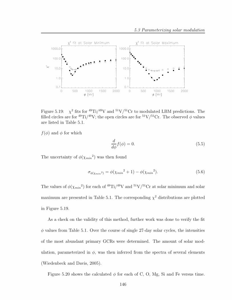
5.3 Parameterizing solar modulation
Figure 5.19: χ2 fits for 49Ti/49V and 51V/51Cr to modulated LBM predictions. Thefilled circles are for 49Ti/49V; the open circles are for 51V/51Cr. The observed φ valuesare listed in Table 5.1.
f(φ) and φ for which
d
dφf(φ) = 0. (5.5)
The uncertainty of φ(χmin2) was then found
σφ(χmin2) = φ(χmin
2 + 1) − φ(χmin2). (5.6)
The values of φ(χmin2) for each of 49Ti/49V and 51V/51Cr at solar minimum and solar
maximum are presented in Table 5.1. The corresponding χ2 distributions are plotted
in Figure 5.19.
As a check on the validity of this method, further work was done to verify the fit
φ values from Table 5.1. Over the course of single 27-day solar cycles, the intensities
of the most abundant primary GCRs were determined. The amount of solar mod-
ulation, parameterized in φ, was then inferred from the spectra of several elements
(Wiedenbeck and Davis, 2005).
Figure 5.20 shows the calculated φ for each of C, O, Mg, Si and Fe versus time.
146

5.3 Parameterizing solar modulation
Figure 5.20: Inferred φ from 27-day average spectral fits of C, O, Mg, Si and Fe.The dashed box is bounded by the best-fit φ±σφ for 51V/51Cr. The dotted box coversthe same region for the 51V/51Cr abundance ratio.
The φ inferred during the period of solar minimum agrees very well with the areas
denoted by the values of φ as determined by the 49Ti/49V and 51V/51Cr abundance
ratios. Although the error bars are considerably larger during the period of solar
maximum, the spread in φ inferred from the spectral fits is mostly contained within
1 σ of the values defined by the electron-capture decay secondaries.
147

Chapter 6
Probing reacceleration with theGALPROP propagation model
6.1 Reacceleration in electron-capture decay sec-
ondaries
As was evidenced by the results presented in §5, the daughter-to-parent abundance
ratios for 49Ti/49V and 51V/51Cr are well represented by our somewhat simple leaky-
box model approximation. Were reacceleration to have been implemented in our
LBM, the effect would have been a shift up in energy of the feature visible in both
ratios at solar minimum. In the cases of both 49V and 51Cr, essentially no reacceler-
ation is required to arrive at reasonable values of the solar modulation parameter φ
as presented in Table 5.1.
The comparison of 51V to heavier parent isotopes by fragmentation presented in
Figure 5.14 is the only indication in the mass-49 and mass-51 reactions that some
degree of reacceleration may be at work in the interstellar medium. While this un-
derestimation of the abundance of 51V could well be the result of inaccurate cross
section measurements in our LBM, it may be that the 51V that was produced by
148

6.2 The GALPROP code
the EC decay of 51Cr at lower energies in the interstellar medium could have been
boosted to a higher energy before being modulated in the heliosphere.
An independent study of the possibility of this effect is a good way to probe
further the possibility of reacceleration. The rest of this chapter is therefore devoted
to presenting the results from our work with the GALPROP convection / diffusion model.
6.2 The GALPROP code
The GALPROP program is a Galactic cosmic-ray numerical propagation code written
mostly in C++ and some FORTRAN. Its design began in 1997 by Igor Moskalenko of the
NASA/Goddard Space Flight Center in Greenbelt, Maryland and Andrew Strong of
the Max-Planck-Institut fur extraterrestrishe Physik in Garching, Germany. The orig-
inal philosophy behind GALPROP was the establishmentof an all-encompassing prop-
agation code, incorporating as many realistic experimental phenomena as possible,
as well as the latest theoretical breakthroughs, in one comprehensive program. In
this way, it may be possible to develop a model to reproduce observational data
related to cosmic-ray origin and propagation directly via measurements of nuclei,
electrons and positrons, and indirectly from gamma rays and synchrotron radiation.
The basic propagation mechanisms are momentum-dependent diffusion and convec-
tion. Energy loss, diffusive reacceleration and fragmentation losses are also treated in
momentum space, using realistic distributions for interstellar gas and radiation fields
(Strong and Moskalenko, 1998). The code computes spectra for all stable and long-
149
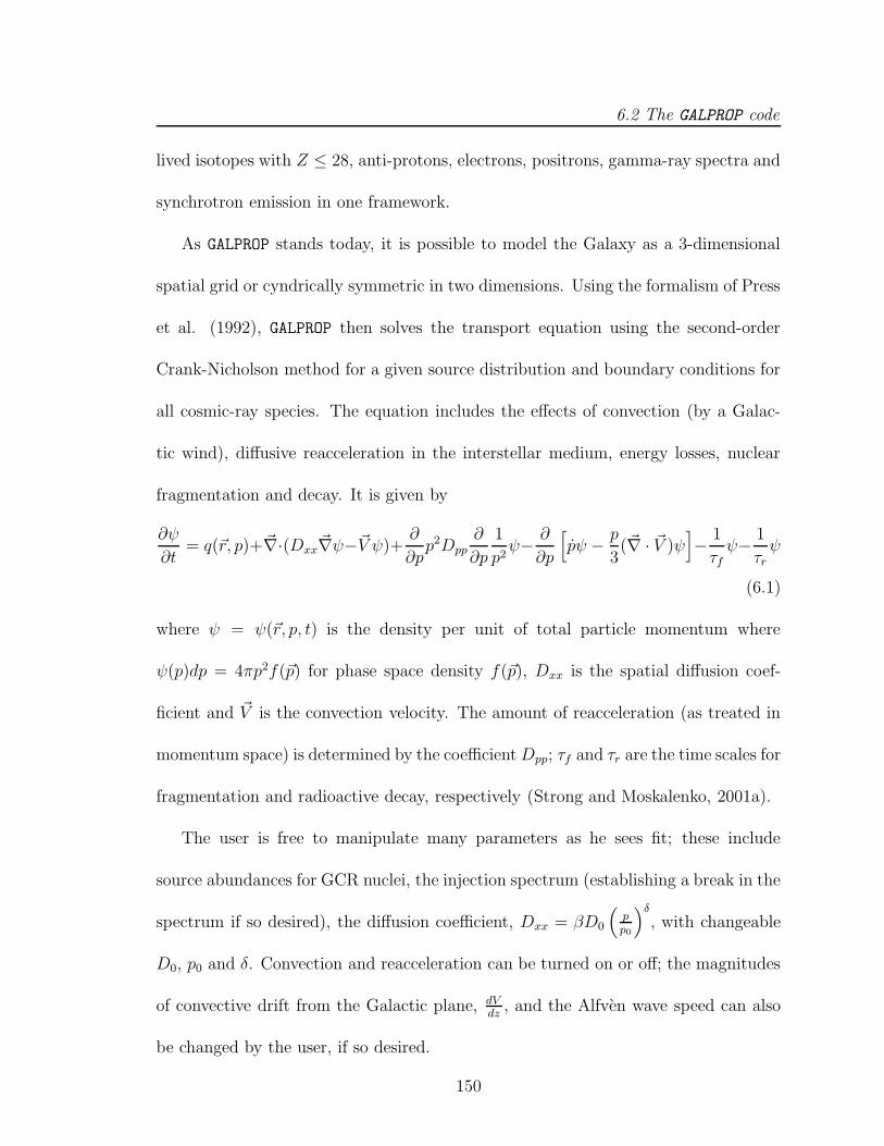
6.2 The GALPROP code
lived isotopes with Z ≤ 28, anti-protons, electrons, positrons, gamma-ray spectra and
synchrotron emission in one framework.
As GALPROP stands today, it is possible to model the Galaxy as a 3-dimensional
spatial grid or cyndrically symmetric in two dimensions. Using the formalism of Press
et al. (1992), GALPROP then solves the transport equation using the second-order
Crank-Nicholson method for a given source distribution and boundary conditions for
all cosmic-ray species. The equation includes the effects of convection (by a Galac-
tic wind), diffusive reacceleration in the interstellar medium, energy losses, nuclear
fragmentation and decay. It is given by
∂ψ
∂t= q(~r, p)+~∇·(Dxx
~∇ψ−~V ψ)+∂
∂pp2Dpp
∂
∂p
1
p2ψ− ∂
∂p
[
pψ − p
3(~∇ · ~V )ψ
]
− 1
τfψ− 1
τrψ
(6.1)
where ψ = ψ(~r, p, t) is the density per unit of total particle momentum where
ψ(p)dp = 4πp2f(~p) for phase space density f(~p), Dxx is the spatial diffusion coef-
ficient and ~V is the convection velocity. The amount of reacceleration (as treated in
momentum space) is determined by the coefficientDpp; τf and τr are the time scales for
fragmentation and radioactive decay, respectively (Strong and Moskalenko, 2001a).
The user is free to manipulate many parameters as he sees fit; these include
source abundances for GCR nuclei, the injection spectrum (establishing a break in the
spectrum if so desired), the diffusion coefficient, Dxx = βD0
(
p
p0
)δ
, with changeable
D0, p0 and δ. Convection and reacceleration can be turned on or off; the magnitudes
of convective drift from the Galactic plane, dVdz
, and the Alfven wave speed can also
be changed by the user, if so desired.
150

6.2 The GALPROP code
The current version has been updated from those previous to include cross-section
measurements and energy-dependent fitting functions as described in Strong and
Moskalenko (2001b). The isotopic cross section database consists of more than 2000
points collected from sources published between 1969 and 1999, including those of
Webber et al. (1990; 1998b; 1998c), Knott et al. (1997) and Chen et al. (1997).
When necessary, theoretical fits scaled to experimental values are implemented based
on Moskalenko and Mashnik (2003), Silberberg et al. (1998), and the work of
Barashenkov et al. (1993; 1994).
The code begins at the heaviest isotope, 64Ni, and solves the propagation equation,
continuously computing the resulting secondary source functions. It then proceeds to
the next lightest isotope until it reaches hydrogen. This iteration is then repeated,
allowing tertiary production and the decay of any short-lived unstable isotopes created
during the first iteration. The effects of electron-capture decay are, of course, included
in the algorithm using a similar technique to that discussed in §4.
The spectrum for any isotope in the GCRs can then be extracted in 1 kpc steps
along the radius of the Galaxy. For our purposes, the spectra were interpolated
between 8 and 9 kpc to arrive at our solar system at ∼ 8.5kpc. The spectra are then
modulated to 1 AU using the Fisk method discussed in §1.2
151

6.3 Three GALPROP models
6.3 Three GALPROP models
This section will present the three basic GALPROP models used to probe the possible
effects of reacceleration on the daughter-to-parent abundance ratios for the EC decay
reactions of 49V and 51Cr. In each case, the user-defined values will be given and the
results of each propagation compared to the parents and daughters in the reactions
and their respective significant channels of production by spallation. The method
and motivation for this work was inspired by the work of Moskalenko et al. (2002).
6.3.1 Plain Diffusion model
Parameters for Plain diffusion modelInjection Index (γ1 / γ2) 2.10 / 2.16a
D0 [cm2 s−1] 2.8 × 1028
Diffusion index (δ1 / δ2) -0.90 / 0.60b
vA [km s−1] N/AdVdz
[km s−1 kpc−1] N/A
Table 6.1: Parameters for the Plain Diffusion Model.(a) for a power-law in rigidity ∝ p−γ; γ1 for p ≤ 20 GV, γ2 for p ≥ 20 GV.
(b) for Dxx = βD0
(
p
p0
)δ
; p0 = 4 GV; δ1 for p ≤ p0, δ2 for p ≥ p0.
The “plain diffusion” model presented here is the best possible reproduction of
a basic leaky-box model: no convection or reacceleration have been applied. The
negative value for the diffusion index at low rigidities correponds to an increase in
the Dxx with decreasing energy. This effect gives a similar result to that described by
Equation 5.3 where the pathlength decreases at low energies. The net effect for GCR
primaries in both cases is a “faster” transit through the Galaxy with correspondingly
152

6.3 Three GALPROP models
Figure 6.1: B/C and (Sc+Ti+V)/Fe at solar minimum with a GALPROP plain diffusionmodel.filled circles: CRIS data (this work).open circles: HEAO-3-C2 data (Engelmann et al., 1990).dashed curve: the unmodulated interstellar value.solid curves: the GALPROP plain diffusion model with solar modulation parametersφ = 350, 400, 500, and 600 MV, corresponding to what one would expect duringsolar minimum.
fewer opportunities for spallation giving rise to fewer secondary nuclei.
The parameters were fine-tuned to secure good agreement with CRIS and HEAO-
3-C2 data for B/C and (Sc+Ti+V)/Fe. Figure 6.1 shows a plot each of these
secondary-to-primary abundance ratios. In both cases, the model agrees quite well
with the abundance ratios; the peaks at around 1 GeV/nucleon are also well repre-
sented by this GALPROP model.
In addition, the GALPROP model of the electron-capture decay daughter-to-parent
abundance ratios for both 49V and 51Cr are in good agreement with the data (see
Figure 6.2). As was the case with the leaky-box model, the cross section for production
of 49Ti for this model also resulted in an overproduction of 49Ti. All production cross
sections for 49Ti have been decreased by 20% in this model (a greater decrease by 5%
153

6.3 Three GALPROP models
Figure 6.2: 49Ti/49V and 51V/51Cr at solar minimum with a GALPROP plain diffusionmodel.dashed curve: the unmodulated interstellar value.solid curves: the GALPROP plain diffusion model with solar modulation parametersφ = 350, 400, 500, and 600 MV, corresponding to what one would expect duringsolar minimum.
over the LBM). Applying the same χ2 fitting routine as we did for the leaky-box model
in §5.3, the 49Ti/49V data correspond to φ = 513.2 ± 64.6 MV while the 51V/51Cr
data correspond to φ = 757.4±119.9 MV during the period of solar minimum. These
values are in somewhat good agreement with each other. Only the φ represented by
49Ti/49V, however, is in good agreement with the values derived from the leaky-box
model in the previous chapter.
If the cross sections for all production channels for 51Cr are increased by 20% and
those for 51V are decreased by 20% (which is reasonable given the large uncertainties
expected from these measurements), the 51V/51Cr abundance ratio is consistent with
φ = 518.0 ± 63.9 MV, and furthermore also in good agreement with the leaky-box
model prediction.
Figures 6.3 and 6.4 show the abundance ratios at solar minimum for 49Ti, 49V,
154

6.3 Three GALPROP models
51V and 51Cr versus the heavier isotopes responsible for most of their production by
spallation. The GALPROP model is in good agreement with the data in most cases for
49V, 49Ti and 51Cr. Whereas we noted that, in the case of the LBM comparison in
Figure 5.14, the model underestimated the values of 51V/55Mn and 51V/56Fe, Figure
6.4 demonstrates that the agreement is much better for these ratios, and that the
model may even tend to overestimate the ratio of 51V to the heavier isotopes. Ad-
justments of the daughter cross sections down by 20% and the parent cross sections
up by 20% begin to resolve this problem in both reactions. In the end, this plain
diffusion model with no reacceleration fits the CRIS data well.
155

6.3 Three GALPROP models
Figure 6.3: The abundance ratios of 49Ti and 49V to their parent isotopes viaproduction by spallation at solar minimum in the context of a GALPROP plain diffusionmodel.dashed curve: the unmodulated interstellar value.solid curves: the GALPROP plain diffusion model with solar modulation parametersφ = 350, 400, 500, and 600 MV, corresponding to what one would expect duringsolar minimum.
156

6.3 Three GALPROP models
Figure 6.4: The abundance ratios of 51V and 51Cr to their parent isotopes viaproduction by spallation at solar minimum in the context of a GALPROP plain diffusionmodel.dashed curve: the unmodulated interstellar value.solid curves: the GALPROP plain diffusion model with solar modulation parametersφ = 350, 400, 500, and 600 MV, corresponding to what one would expect duringsolar minimum.
157

6.3 Three GALPROP models
6.3.2 Diffusive Reacceleration model
Parameters for Diffusive Reacceleration modelInjection Index (γ1 / γ2) 2.10 / 2.42a
D0 [cm2 s−1] 6.5 × 1028
Diffusion index (δ) 0.33vA [km s−1] 35
dVdz
[km s−1 kpc−1] N/A
Table 6.2: Parameters for the Diffusive Reacceleration Model.(a) for a power-law in rigidity ∝ p−γ; γ1 for p ≤ 9 GV, γ2 for p ≥ 9 GV.
This diffusive reacceleration model is based on the previous work of Strong et
al. (1998) and Moskalenko et al. (2002). It was found that a diffusion coefficient
taking the form of a Kolmogorov spectrum of interstellar turbulence (δ = 13), given
by Dxx = 6.5 × 1028β( p
4 GV)
13 , agreed well with the B/C ratio for both the lower en-
ergy CRIS data and for the higher energy HEAO-3-C2 data (Engelmann et al., 1990;
de Nolfo et al., 2005). The injection spectrum index above 9 GV is considerably
steeper than the normally accepted index of about -2.1. The peak in the B/C ratio
was well-defined by a model with an Alfven speed of 35 km/s and a Galactic halo size
of 4 kpc, based on constraints found from measurements of the radioactive isotopes
10Be, 26Al, 36Cl and 54Mn (Strong and Moskalenko, 2001b). This halo size remains
unchanged for all three models discussed here.
Figure 6.5 shows the abundance ratios B/C and (Sc+Ti+V)/Fe in the context
of our GALPROP diffusive reacceleration model. Though this model does not agree
as well at higher energies as our plain diffusion model, the CRIS data are relatively
well-described by the diffusive reacceleration model.
158

6.3 Three GALPROP models
Figure 6.5: B/C and (Sc+Ti+V)/Fe at solar minimum with a GALPROP diffusivereacceleration model.filled circles: CRIS data (this work).open circles: HEAO-3-C2 data (Engelmann et al., 1990).dashed curve: the unmodulated interstellar value.solid curves: the GALPROP diffusive reacceleration model with solar modulation pa-rameters φ = 350, 400, 500, and 600 MV, corresponding to what one would expectduring solar minimum.
Figure 6.6 shows the 49Ti/49V and 51V/51Cr abundance ratios at solar minimum
in the context of this diffusive reacceleration model. In order to secure better agree-
ment with the electron-capture decay abundance ratios, the spallation cross sections
for all production channels for the parent isotopes, 49V and 51Cr, have been increased
by 20%; the cross sections for the daughters, 49Ti and 51V, have also been decreased
by 20%. Changes by this magnitude are reasonable with respect to the uncertain-
ties expected for these measurements. Even with changes to the cross sections, the
effect of reacceleration in the ISM is immediately evident in this model: the model
overestimates the abundance ratios in both cases. The effect of reacceleration is also
present in Figures 6.7 and 6.8. Both the 49V and 49Ti ratios are overestimated in
all cases by the diffusive reacceleration model. The modeling of the mass-51 ratios
159

6.3 Three GALPROP models
remain somewhat unchanged from their values in the plain diffusion case, but are in
slightly worse agreement in this case.
Applying a χ2 fit to each of these ratios, the 49Ti/49V ratio is consistent with
φ = 674.2 ± 100.3 MV and the 51V/51Cr ratio is best fit by φ = 904.1 ± 127.3 MV.
Without the adjustments applied to the cross sections (leaving only the production
cross sections for 49Ti decreased by 20%), the χ2 fit results in φ = 843.0 ± 112.5 MV
for 49Ti/49V and φ = 1429.7 ± 208.9 MV for 51V/51Cr. Kinetic energy per nucleon,
E is related to rigidity, R, by the relation
E = −M0 +
√
M02 +R2
Z2
A2(6.2)
where M0 is the mass of a nucleon. This corresponds to a possible energy boost in
this reacceleration model of several tens to 100 MeV/nucleon over what was seen in
the plain diffusion model.
160

6.3 Three GALPROP models
Figure 6.6: 49Ti/49V and 51V/51Cr at solar minimum with a GALPROP diffusive reac-celeration model.dashed curve: the unmodulated interstellar value.solid curves: the GALPROP diffusive reacceleration model with solar modulation pa-rameters φ = 350, 400, 500, and 600 MV, corresponding to what one would expectduring solar minimum.
6.3.3 Diffusion / Convection with Minimal Reacceleration
Parameters for Diffusion / Convection modelwith Minimal Reacceleration
Injection Index (γ1 / γ2) 2.10 / 2.25a
D0 [cm2 s−1] 3.0 × 1028
Diffusion index (δ) 0.50vA [km s−1] 20
dVdz
[km s−1 kpc−1] 10
Table 6.3: Parameters for the Diffusion / Convection model with Minimal Reaccel-eration.(a) for a power-law in rigidity ∝ p−γ; γ1 for p ≤ 9 GV, γ2 for p ≥ 9 GV.
This model was motivated by the work of Moskalenko et al. (2003) and Ptuskin
et al. (2003) and references therein. It is based on an Iroshnikov-Kraichnan model
(δ = 12) for the diffusion of cosmic rays in the ISM with the coefficient taking the
form Dxx = 3.0 × 1028β(
p
4 GV
)12 . The Alfven speed has been decreased to 20 km/s
from 35 km/s in the previous model and we have included convective drift out of the
161

6.3 Three GALPROP models
Figure 6.7: The abundance ratios of 49Ti and 49V to their parent isotopes viaproduction by spallation at solar minimum in the context of a GALPROP diffusive reac-celeration model.dashed curve: the unmodulated interstellar value.solid curves: the GALPROP diffusive reacceleration model with solar modulation pa-rameters φ = 350, 400, 500, and 600 MV, corresponding to what one would expectduring solar minimum.
162

6.3 Three GALPROP models
Figure 6.8: The abundance ratios of 51V and 51Cr to their parent isotopes viaproduction by spallation at solar minimum in the context of a GALPROP diffusive reac-celeration model.dashed curve: the unmodulated interstellar value.solid curves: the GALPROP diffusive reacceleration model with solar modulation pa-rameters φ = 350, 400, 500, and 600 MV, corresponding to what one would expectduring solar minimum.
163

6.3 Three GALPROP models
plane of the Galaxy amounting to dVdz
= 10 km s−1 kpc−1.
It was shown in the previously cited works that the interaction and stochastic ac-
celeration of cosmic rays by magnetohydrodynamic waves can result in a “damping”
of the interstellar turbulence responsible for the diffusion of GCRs. Using GALPROP
to allow GCR protons to iteratively damp this turbulence starting from both a Kol-
mogorov and Iroshnikov-Kraichnan model, it was shown that this damping is prob-
lematic for the Iroshnikov-Kraichnan case but not in the Kolmogorov case.
Figure 6.9 shows the results for the B/C and (Sc+Ti+V)/Fe ratios in the context
of this diffusion / convection model with minimal reacceleration (no wave damping
effects have been implemented in the code). It is evident, especially in the case of
B/C, that some wave damping may be needed to increase the diffusion coefficient at
low energies, thereby decreasing the production of Boron.
In order to simulate this wave damping effect in the Iroshnikov-Kraichnan model,
we tried implementing a break in the diffusion coefficient similar to what was done in
the plain diffusion model: δ1 = 0.30 below a particle ridigity of 4 GV and δ2 = 0.50
above 4 GV. Figure 6.10 shows B/C and (Sc+Ti+V)/Fe in the context of this “wave-
damped” diffusion / convection model with minimal reacceleration. While the model
does not agree that well in the case of B/C, the model is in good agreement with the
low-energy sub-Fe/Fe ratio. All references to the diffusion / convection model with
minimal reacceleration hereafter will include the model with simulated wave damping.
It was found that both 49Ti and 51V were overproduced by this model. We have
reduced all cross sections for production of both of these daughter isotopes by 20%
164

6.3 Three GALPROP models
Figure 6.9: B/C and (Sc+Ti+V)/Fe at solar minimum with a GALPROP diffusion /convection model with minimal reacceleration.filled circles: CRIS data (this work).open circles: HEAO-3-C2 data (Engelmann et al., 1990).dashed curve: the unmodulated interstellar value.solid curves: the GALPROP diffusion / convection model with minimal reaccelerationwith solar modulation parameters φ = 350, 400, 500, and 600 MV, corresponding towhat one would expect during solar minimum.
Figure 6.10: B/C and (Sc+Ti+V)/Fe at solar minimum with a GALPROP “wave-damped” diffusion / convection model with minimal reacceleration.filled circles: CRIS data (this work).open circles: HEAO-3-C2 data (Engelmann et al., 1990).dashed curve: the unmodulated interstellar value.solid curves: the GALPROP diffusion / convection model with minimal reaccelerationwith solar modulation parameters φ = 350, 400, 500, and 600 MV, corresponding towhat one would expect during solar minimum.
165

6.3 Three GALPROP models
in this study. Figure 6.11 shows the 49Ti/49V and 51V/51Cr abundance ratios in
the context of this “wave-damped” model. For the mass-49 ratio, this model agrees
slightly better at higher energies than for the diffusive reacceleration model. The
51V/51Cr prediction agrees much better in this case than for the diffusive reaccelera-
tion case. On the whole, as expected, the effect of reacceleration is smaller with this
model. After computing a χ2 fit to the results, we see that 49Ti/49V is best fit by
φ = 645.8 ± 74.9 MV, and 51V/51Cr is consistent with φ = 718.2 ± 91.2 MV.
Figures 6.12 and 6.13 show the ratios of the parents and daughters to their primary
progenitors by spallation. The model is in systematically better agreement with the
49V ratios than it was in the diffusive reacceleration case. The model is also in much
better agreement with the 49Ti ratios, due in part to the reduction in cross section
mentioned previously. In the case of 51Cr, the ratios remain essentially unchanged
from their values in the diffusive reacceleration model; the 51V ratios are pulled down,
in slightly better agreement than the previous model.
166

6.4 Summary of comparisons with GALPROP
Figure 6.11: 49Ti/49V and 51V/51Cr at solar minimum with a GALPROP “wave-damped” diffusion / convection model with minimal reacceleration.dashed curve: the unmodulated interstellar value.solid curves: the GALPROP diffusion / convection model with minimal reaccelerationwith solar modulation parameters φ = 350, 400, 500, and 600 MV, corresponding towhat one would expect during solar minimum.
6.4 Summary of comparisons with GALPROP
The previous three GALPROP models give the best possible fits of three different
GALPROP propagation models to the CRIS data. In the case of the plain diffusion
model, the best fit required the reduction of both daughter isotopes production cross
sections by 20% and the increase of the 51Cr production cross sections by 20%. For
the diffusive reacceleration model, these same adjustments to the cross sections were
made, in addition to the increase of the 51V production cross sections by 20%. The
diffusion / convection model with minimal reacceleration, however, required only a
decrease by 20% of the production cross sections for the daughter isotopes, 49Ti and
51V.
As can be seen in Figure 6.2, the simple plain diffusion model with no reaccel-
167

6.4 Summary of comparisons with GALPROP
Figure 6.12: The abundance ratios of 49Ti and 49V to their parent isotopes via pro-duction by spallation at solar minimum in the context of a GALPROP “wave-damped”diffusion / convection model with minimal reacceleration.dashed curve: the unmodulated interstellar value.solid curves: the GALPROP diffusion / convection model with minimal reaccelerationwith solar modulation parameters φ = 350, 400, 500, and 600 MV, corresponding towhat one would expect during solar minimum.
168

6.4 Summary of comparisons with GALPROP
Figure 6.13: The abundance ratios of 51V and 51Cr to their parent isotopes via pro-duction by spallation at solar minimum in the context of a GALPROP “wave-damped”diffusion / convection model with minimal reacceleration.dashed curve: the unmodulated interstellar value.solid curves: the GALPROP diffusive reacceleration model with solar modulation pa-rameters φ = 350, 400, 500, and 600 MV, corresponding to what one would expectduring solar minimum.
169

6.4 Summary of comparisons with GALPROP
eration agrees very well with both abundance ratios, and is consistent with a φ of
∼ 500 MV. This model is in very good agreement with the results we obtained with
our simple leaky-box model.
Although the two reacceleration models are based on quite different diffusion
models, their results are similar. In both cases, the results of reacceleration are as
expected: the calculated daughter-to-parent abundance ratios appear to be shifted
upward in energy. The data, as a result, are consistent with a level of solar modulation
of ∼ 150 to 400 MV more than that given by the plain diffusion model, indicating
(by Equation 6.2) an apparent boost in the interstellar medium of several tens of
MeV/nucleon (see Table 6.4).
Figure 6.14 shows the range of φ (bound by φ± σφ) corresponding to the best-fit
φ based on inferences on the spectral fits of C, O, Mg, Si and Fe and the best-fit φ
from comparisons of 49Ti/49V and 51V/51Cr to the leaky-box model, as discussed in
§5, and the three GALPROP models, during the solar minimum period. The best-fit φ
from comparisons of the mass-49 and mass-51 electron-capture-decay reactions to the
LBM and the GALPROP plain diffusion model agree quite well with the φ inferred from
spectral fits. In the cases of the diffusive reacceleration model and the convection /
49Ti/49V 51V/51CrPD 513.2 ± 64.6 MV 518.0 ± 63.9 MVDR 674.2 ± 100.3 MV 904.1 ± 127.3 MV
DCMR 645.8 ± 74.9 MV 718.2 ± 91.2 MV
Table 6.4: Values of φ from fits of 49Ti/49V and 51V/51Cr to the GALPROP plaindiffusion model, diffusive reacceleration model and diffusion / convection model withminimal reacceleration.
170
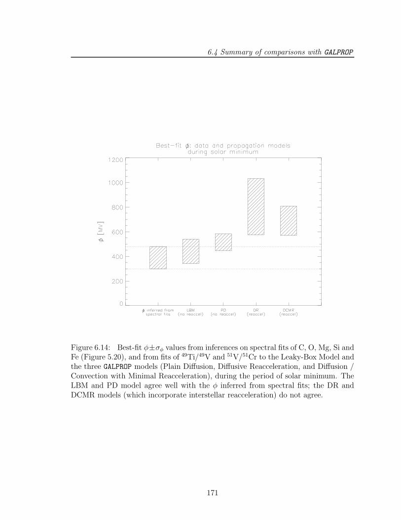
6.4 Summary of comparisons with GALPROP
Figure 6.14: Best-fit φ±σφ values from inferences on spectral fits of C, O, Mg, Si andFe (Figure 5.20), and from fits of 49Ti/49V and 51V/51Cr to the Leaky-Box Model andthe three GALPROP models (Plain Diffusion, Diffusive Reacceleration, and Diffusion /Convection with Minimal Reacceleration), during the period of solar minimum. TheLBM and PD model agree well with the φ inferred from spectral fits; the DR andDCMR models (which incorporate interstellar reacceleration) do not agree.
171

6.4 Summary of comparisons with GALPROP
diffusion model with minimal reacceleration, however, a larger value of φ is necessary
to secure good agreement with the range of φ estimated from the primary GCR
spectral fits. The best-fit φ values from the reacceleration models are significantly
higher than what one would expect for the value of φ during solar minimum by ∼ 300
to ∼ 800 MV.
Since the effects of solar modulation and interstellar reacceleration are essentially
inverse processes, the increase in φ calculated from the reacceleration models relative
to the leaky-box and plain diffusion models is tantamount to a increase of several tens
to 100 MeV/nucleon in the GCR interstellar energies in the reacceleration models (by
Equation 6.2). While inaccurate data for the production cross sections could play a
role in the apparent overestimation of the abundance ratios in the reacceleration
models, it is unlikely that more accurate experimental data for these cross sections
will change the outcome significantly. It is evident that the inclusion of little or no
reacceleration is necessary to correctly predict the values of the electron-capture-decay
daughter-to-parent abundance ratios at solar minimum.
172

Chapter 7
Conclusions
This dissertation has examined electron-capture secondary isotopes in the Galactic
cosmic rays. Results of this analysis include new direct evidence for changes in the
amount of energy-loss that cosmic rays suffer in the heliosphere from solar minimum
to solar maximum. Comparing measurements with a leaky-box propagation model,
we have quantified the magnitude of this energy loss. Following a further comparison
of our electron-capture decay measurements to a set of GALPROP propagation models
incorporating varying amounts of reacceleration, we have concluded that the model
requires little or no reacceleration to correctly predict the observed energy-dependence
of the daughter-to-parent abundance ratios at solar minimum.
7.1 Improvements on the analysis methods
This dissertation has presented methods for making improvements on previous work,
i.e. (Niebur et al., 2003), in the methods of analyzing CRIS data for the purposes
of generating accurate isotopic spectra and abundance ratios for 70 isotopes between
5 ≤ Z ≤ 28. A detailed method for performing a maximum-likelihood multiple-
173
7.2 Direct evidence of cosmic-ray energy loss in the heliosphere
Gaussian peak-fitting routine designed to obtain better fits for data with low statistics
has been discussed and the code for a program in C has been given (see Appendix A).
We have provided a technique for avoiding the problems associated with comparing
isotopes of similar range but different energies (Appendix B). Additionally, we have
developed a Monte-Carlo routine for determining the appropriate geometry factor for
a given isotope and have demonstrated the use of the bowtie method to identify the
best energy value for a given isotope in a given detector (Appendices C and D).
7.2 Direct evidence of cosmic-ray energy loss in
the heliosphere
We have demonstrated with the electron-capture decay daughter-to-parent abundance
ratios, 49Ti/49V and 51V/51Cr, that significant electron-capture decay does occur
before these cosmic rays enter the heliosphere. In §5, we compared our results to
a leaky-box model for Galactic cosmic-ray propagation which includes a numerical
calculation of a spherically symmetric Fokker-Planck equation to simulate diffusion,
convection and adiabatic energy loss in the heliosphere. We conclude that during the
period of solar minimum, the data are consistent with a solar modulation parameter,
φ of about 350 to 500 MV, while during solar maximum, φ is about 750 to 1100
MV. In addition, we have independently verified our method by showing that these
measurements of φ agree well with values of φ inferred from fitting the spectra of the
GCR primary elements C, O, Mg, Si and Fe.
174

7.3 No evidence of reacceleration
7.3 No evidence of reacceleration
Using the Galactic cosmic-ray numerical propagation code, GALPROP, we have com-
pared the 49Ti/49V and 51V/51Cr abundance ratios to three very different GCR prop-
agation models. Using a plain diffusion model similar to our leaky-box model, we
have shown independently that the energy-dependence of both electron-capture-decay
abundance ratios are consistent with a φ of about 500 MV during the period of solar
minimum. We have also shown that two different GALPROP models incorporating dif-
fering amounts of reacceleration require a best-fit solar modulation parameter φ for
the electron-capture-decay ratios 49Ti/49V and 51V/51Cr that is ∼ 300 to ∼ 800 MV
higher during solar minimum than the φ inferred from spectral fits of the GCR pri-
mary elements C, O, Mg, Si and Fe. This increase in φ is consistent with an energy
boost of several tens to 100 MeV/nucleon in the reacceleration models relative to the
models that do not incorporate any interstellar reacceleration. We conclude that little
or no interstellar reacceleration is required to correctly model the observed electron-
capture-decay daughter-to-parent abundance ratios.
175

Bibliography
Abbasi, R. U., Abu-Zayyad, T., Amann, J. F., Archbold, G., Atkins, R., Bellido, J. A.,Belov, K., Belz, J. W., BenZvi, S., Bergman, D. R., Boyer, J. H., Burt, G. W.,Cao, Z., Clay, R. W., Connolly, B. M., Dawson, B. R., Deng, W., Fedorova, Y.,Findlay, J., Finley, C. B., Hanlon, W. F., Hoffman, C. M., Holzscheiter, M. H.,Hughes, G. A., Huntemeyer, P., Jui, C. C. H., Kim, K., Kirn, M. A., Knapp, B. C.,Loh, E. C., Maestas, M. M., Manago, N., Mannel, E. J., Marek, L. J., Martens,K., Matthews, J. A. J., Matthews, J. N., O’Neill, A., Painter, C. A., Perera,L., Reil, K., Riehle, R., Roberts, M. D., Sasaki, M., Schnetzer, S. R., Seman,M., Simpson, K. M., Sinnis, G., Smith, J. D., Snow, R., Sokolsky, P., Song, C.,Springer, R. W., Stokes, B. T., Thomas, J. R., Thomas, S. B., Thomson, G. B.,Tupa, D., Westerhoff, S., Wiencke, L. R., and Zech, A.: 2004a, Astrophys. J. 610,L73
Abbasi, R. U., Abu-Zayyad, T., Amann, J. F., Archbold, G., Bellido, J. A., Belov,K., Belz, J. W., Bergman, D. R., Cao, Z., Clay, R. W., Cooper, M. D., Dai, H.,Dawson, B. R., Everett, A. A., Fedorova, Y. A., Girard, J. H., Gray, R. C., Hanlon,W. F., Hoffman, C. M., Holzscheiter, M. H., Huntemeyer, P., Jones, B. F., Jui,C. C., Kieda, D. B., Kim, K., Kirn, M. A., Loh, E. C., Manago, N., Marek, L. J.,Martens, K., Martin, G., Matthews, J. A., Matthews, J. N., Meyer, J. R., Moore,S. A., Morrison, P., Moosman, A. N., Mumford, J. R., Munro, M. W., Painter,C. A., Perera, L., Reil, K., Riehle, R., Roberts, M., Sarracino, J. S., Sasaki, M.,Schnetzer, S. R., Shen, P., Simpson, K. M., Sinnis, G., Smith, J. D., Sokolsky, P.,Song, C., Springer, R. W., Stokes, B. T., Taylor, S. F., Thomas, S. B., Thompson,T. N., Thomson, G. B., Tupa, D., Westerhoff, S., Wiencke, L. R., Vanderveen,T. D., Zech, A., and Zhang, X.: 2004b, Physical Review Letters 92(15), 151101
Allbritton, G. A., Anderson, H., Barnes, A., Christian, E. R., Cummings, A. C.,Dougherty, B. L., Jensen, L., Lee, J., Leske, R. A., Madden, M. P., Mewaldt,R. A., Milliken, B., Nahory, B. W., O’Donnell, R., Schmidt, P., Sears, B. R., vonRosenvinge, T. T., Walton, J. T., Wiedenbeck, M. E., and Wong, Y. K.: 1996,IEEE Trans. Nucl. Sci. 43, 1505
Andersen, H. H. and Ziegler, Z. F.: 1977, The Stopping and Ranges of Ions in Matter,Pergamon, New York
Barashenkov, V. S.: 1993, Dubna, Joint Institute for Nuclear ResearchBarashenkov, V. S. and Polanski, A.: 1994, Comm. JINR E2-94-417, Dubna, Joint
Institute for Nuclear Research
176

BIBLIOGRAPHY
Binns, W. R., Wiedenbeck, M. E., Arnould, M., Cummings, A. C., George, J. S.,Goriely, S., Israel, M. H., Leske, R. A., Mewaldt, R. A., Meynet, G., Scott, L. M.,Stone, E. C., and von Rosenvinge, T. T.: 2005, in progress
Casse, M. and Goret, P.: 1978, Astrophys. J. 221, 703Casse, M. and Paul, J. A.: 1982, Astrophys. J. 258, 860Chen, C.-X., Albergo, S., Caccia, Z., Costa, S., Crawford, H. J., Cronqvist, M.,
Engelage, J., Greiner, L., Guzik, T. G., Insolia, A., Knott, C. N., Lindstrom,P. J., McMahon, M., Mitchell, J. W., Potenza, R., Russo, G. V., Soutoul, A.,Testard, O., Tull, C. E., Tuve, C., Waddington, C. J., Webber, W. R., and Wefel,J. P.: 1997, Phys. Rev. C. 56, 1536
Compton, A. H.: 1933, Phys. Rev. 41, 111Connell, J. J.: 2001, Space Science Reviews 99, 41Connell, J. J. and Simpson, J. A.: 1999, Proceedings of the 26th International Con-
ference on Cosmic Rays, held in Salt Lake City, Utah, 17-25 August, 1999 3,33
Cowsik, R., Pal, Y., Tandon, S. N., and Verma, R. P.: 1967, Phys. Rev. 158, 1238Crawford, H. J.: 1979, Ph.D. thesis, University of California, Berkeley, Lawrence
Berkeley Laboratory Report LBL-8807Cronin, J., Gaisser, T. K., and Swordy, S. P.: 1997, Scientific American 276, 44Davis, A. J., Mewaldt, R. A., Cohen, C. M. S., Cummings, A. C., George, J. S.,
Leske, R. A., Stone, E. C., Wiedenbeck, M. E., Yanasak, N. E., Christian, E. R.,von Rosenvinge, T. T., Binns, W. R., and Hink, P. L.: 2001, J. Geophys. Res.106, 29979
de Nolfo, G. A., Moskalenko, I. V., Binns, W. R., Cummings, A. C., Davis, A. J.,George, J. S., Hink, P. L., Israel, M. H., Leske, R. A., Lijowski, M., Mewaldt,R. A., Stone, E. C., Strong, A. W., von Rosenvinge, T. T., Wiedenbeck, M. E.,and Yanasak, N. E.: 2005, in progress
Derrickson, J. H., Parnell, T. A., Austin, R. W., Selig, W. J., and Gregory, J. C.:1992, International Journal of Radiation Applications and Instrumentation DNuclear Tracks and Radiation Measurements 20, 415
Duvernois, M. A. and Thayer, M. R.: 1996, Astrophys. J. 465, 982Engelmann, J. J., Ferrando, P., Soutoul, A., Goret, P., and Juliusson, E.: 1990,
Astron. Astrophys. 233, 96Etchegoyen, A.: 2004, Astrophys. Space Sci. 290, 379Fisk, L. A.: 1971, J. Geophys. Res. 76, 221Fisk, L. A., Kozlovsky, B., and Ramaty, R.: 1974, Astrophys. J. 190, L35Fisk, L. A., Ramaty, R., and Goldstein, M. L.: 1971, Proceedings of the 12th Inter-
national Conference on Cosmic Rays, held in Tasmania, Australia, 16-25 August,1971. Volume 2., p.799 2, 799
Foukal, P.: 1990, Solar astrophysics, New York, Wiley-Interscience, 1990, 492 p.Gahbauer, F., Hermann, G., Horandel, J. R., Muller, D., and Radu, A. A.: 2004,
Astrophys. J. 607, 333Garcia-Munoz, M., Mason, G. M., Simpson, J. A., and Wefel, J. P.: 1977, Proceedings
177

BIBLIOGRAPHY
of the 15th International Conference on Cosmic Rays, held in Plovdiv, Volume 11, 230
George, J. S., Binns, W. R., Christian, E. R., Cummings, A. C., Davis, A. J., deNolfo, G. A., Hink, P. L., Israel, M. H., Leske, R. A., Lijowski, M., Mewaldt,R. A., Scott, L. M., Stone, E. C., von Rosenvinge, T. T., Wiedenbeck, M. E., andYanasak, N. E.: 2005, in progress
Ginzburg, V. L. and Syrovatsky, S. I.: 1964, The Origin of Cosmic Rays, Pergamon,Oxford
Gleeson, L. J. and Axford, W. I.: 1968, Astrophys. J. 154, 1011Gloeckler, G., Cain, J., Ipavich, F. M., Tums, E. O., Bedini, P., Fisk, L. A., Zur-
buchen, T. H., Bochsler, P., Fischer, J., Wimmer-Schweingruber, R. F., Geiss, J.,and Kallenbach, R.: 1998, Space Science Reviews 86, 497
Gold, R. E., Krimigis, S. M., Hawkins, S. E., Haggerty, D. K., Lohr, D. A., Fiore, E.,Armstrong, T. P., Holland, G., and Lanzerotti, L. J.: 1998, Space Science Reviews86, 541
Goldstein, M. L., Fisk, L. A., and Ramaty, R.: 1970, Phys. Rev. Lett. 25, 832Greisen, K.: 1966, Phys. Rev. Lett. 16, 748Higdon, J. C. and Lingenfelter, R. E.: 2003, Astrophys. J. 590, 822Higdon, J. C., Lingenfelter, R. E., and Ramaty, R.: 1998, Astrophys. J. 509, L33Janni, J. F.: 1966, Calculations of Energy Loss, Range, Pathlength, Straggling, Multi-
ple Scatter, and the Probability of Inelastic Nuclear Collision for 0.1 to 1000 MeVProtons, AFWL-TR-65-160
Jokipii, J. R. and Levy, E. H.: 1977, Astrophys. J. 213, L85Jokipii, J. R. and Thomas, B.: 1981, Astrophys. J. 243, 1115Knott, C. N., Albergo, S., Caccia, Z., Chen, C.-X., Costa, S., Crawford, H. J., Cron-
qvist, M., Engelage, J., Greiner, L., Guzik, T. G., Insolia, A., Lindstrom, P. J.,Mitchell, J. W., Potenza, R., Russo, G. V., Soutoul, A., Testard, O., Tull, C. E.,Tuve, C., Waddington, C. J., Webber, W. R., and Wefel, J. P.: 1997, Phys. Rev.C. 56, 398
Lawrence, D. J.: 1996, Ph.D. thesis, Washington University in St. LouisLeo, W. R.: 1994, Techniques for Nuclear and Particle Physics Experiments, Second
Revised Edition, Springer-Verlag, BerlinLeske, R. A.: 1993, Astrophys. J. 405, 567Letaw, J. R., Adams, J. H., Silberberg, R., and Tsao, C. H.: 1985, Astrophys. Space
Sci. 114, 365Letaw, J. R., Silberberg, R., and Tsao, C. H.: 1993, Astrophys. J. 414, 601Lezniak, J. A. and Webber, W. R.: 1978, Astrophys. J. 223, 676Link, J. T.: 2003, Ph.D. thesis, Washington University in St. LouisLodders, K.: 2003, Astrophys. J. 591, 1220Longair, M. S.: 1992, High Energy Astrophysics: Particles, photons and their detec-
tion, 2nd edition, Vol. 1, Cambridge University Press, United KingdomLukasiak, A., McDonald, F. B., and Webber, W. R.: 1997, Astrophys. J. 488, 454Mobius, E., Kistler, L. M., Popecki, M. A., Crocker, K. N., Granoff, M., Turco,
178

BIBLIOGRAPHY
S., Anderson, A., Demain, P., Distelbrink, J., Dors, I., Dunphy, P., Ellis, S.,Gaidos, J., Googins, J., Hayes, R., Humphrey, G., Kastle, H., Lavasseur, J.,Lund, E. J., Miller, R., Sartori, E., Shappirio, M., Taylor, S., Vachon, P., Vosbury,M., Ye, V., Hovestadt, D., Klecker, B., Arbinger, H., Kunneth, E., Pfeffermann,E., Seidenschwang, E., Gliem, F., Reiche, K.-U., Stockner, K., Wiewesiek, W.,Harasim, A., Schimpfle, J., Battell, S., Cravens, J., and Murphy, G.: 1998, SpaceScience Reviews 86, 449
Mason, G. M., Gold, R. E., Krimigis, S. M., Mazur, J. E., Andrews, G. B., Daley,K. A., Dwyer, J. R., Heuerman, K. F., James, T. L., Kennedy, M. J., Lefevere,T., Malcolm, H., Tossman, B., and Walpole, P. H.: 1998, Space Science Reviews86, 409
Meneguzzi, M., Audouze, J., and Reeves, H.: 1971, Astron. Astrophys. 15, 337Meyer, J., Drury, L. O., and Ellison, D. C.: 1997, Astrophys. J. 487, 182Meynet, G., Arnould, M., Paulus, G., and Maeder, A.: 2001, Space Science Reviews
99, 73Moskalenko, I. V., Jones, F. C., Mashnik, S. G., Ptuskin, V. S., and Strong, A. W.:
2003, Proceedings of the 28th International Cosmic Ray Conference. July 31-August 7, 2003. Tsukuba, Japan. Under the auspices of the International Union ofPure and Applied Physics (IUPAP). Editors: T. Kajita, Y. Asaoka, A. Kawachi,Y. Matsubara and M. Sasaki, p.1925 28, 1925
Moskalenko, I. V. and Mashnik, S. G.: 2003, Proceedings of the 28th InternationalCosmic Ray Conference. July 31-August 7, 2003. Tsukuba, Japan. Under the aus-pices of the International Union of Pure and Applied Physics (IUPAP). Editors:T. Kajita, Y. Asaoka, A. Kawachi, Y. Matsubara and M. Sasaki, p.1969 28, 1969
Moskalenko, I. V., Strong, A. W., Ormes, J. F., and Potgieter, M. S.: 2002, Astrophys.J. 565, 280
Murdin, P.: 2000, Encyclopedia of Astronomy and AstrophysicsNiebur, S. M.: 2001, Ph.D. thesis, Washington University in St. LouisNiebur, S. M., Scott, L. M., Wiedenbeck, M. E., Binns, W. R., Christian, E. R.,
Cummings, A. C., Davis, A. J., George, J. S., Hink, P. L., Israel, M. H., Leske,R. A., Mewaldt, R. A., Stone, E. C., von Rosenvinge, T. T., and Yanasak, N. E.:2003, J. Geophys. Res. (Space Physics) 108, 8
Orear, J.: 1982, Notes on statistics for Physicists, revised, Cornell University, Ithaca,New York
Osborne, J. L. and Ptuskin, V. S.: 1988, Soviet Astronomy Letters 14, 132Osborne, J. L., Wolfendale, A. W., and Wdowczyk, J.: 1976, Journal of Physics A
Mathematical General 9, 1399Parker, E. N.: 1965, Planet. Space Sci. 13, 9Parker, E. N.: 1966, Planet. Space Sci. 14, 371Parrington, J. R., Knox, H. D., Breneman, S. L., Baum, E. M., and Feiner, F.: 1996,
Nuclides and Isotopes, Fifteenth Edition, General Electric Co.Pesses, M. E., Eichler, D., and Jokipii, J. R.: 1981, Astrophys. J. 246, L85Povh, B., Rith, K., Scholz, C., and Zetsche, F.: 1999, Particles and Nuclei: An
179

BIBLIOGRAPHY
Introduction to the Physical Concepts, 2nd edition, Springer, Berlin, GermanyPress, W. H., Flannery, B. P., Teukolsky, S. A., and Vetterling, W. T.: 1992, Numer-
ical Recipes in FORTRAN, 2nd ed., Cambridge University Press, CambridgePtuskin, V. S., Jones, F. C., Moskalenko, I. V., and Zirakashvili, V. N.: 2003,
Proceedings of the 28th International Cosmic Ray Conference. July 31-August 7,2003. Tsukuba, Japan. Under the auspices of the International Union of Pure andApplied Physics (IUPAP). Editors: T. Kajita, Y. Asaoka, A. Kawachi, Y. Mat-subara and M. Sasaki, p.1929 28, 1929
Raisbeck, G., Perron, C., Toussaint, J., and Yiou, F.: 1973, Proceedings of the 13thInternational Conference on Cosmic Rays, held in Denver, Colorado, Volume 1(OG Sessions)., p.534 1, 534
Raisbeck, G. M., Comstock, G., Perron, C., and Yiou, F.: 1975, Proceedings fromthe 14th International Cosmic Ray Conference, held in Munchen, Germany, 15-29August, 1975. Volume 3 (MG Session)., p.937 3, 937
Rygg, T. A. and Earl, J. A.: 1967, J. Geophys. Res. 76, 7445Seo, E. S., Ahn, H. S., Beatty, J. J., Coutu, S., Choi, M. J., Duvernois, M. A., Ganel,
O., Kang, T. G., Kim, K. C., Lee, M. H., Lutz, L., Marrocchesi, P. S., Minnick, S.,Min, K. W., Nutter, S., Park, H., Park, I. H., Schindhelm, E., Sina, R., Swordy,S., Wu, J., and Yang, J.: 2004, Advances in Space Research 33, 1777
Silberberg, R., Tsao, C. H., and Barghouty, A. F.: 1998, Astrophys. J. 501, 911Silberberg, R., Tsao, C. H., Letaw, J. R., and Shapiro, M. M.: 1983, Physical Review
Letters 51, 1217Smith, A. E.: 1996, http://home.hiwaay.net/∼smithae/cr.htmlSmith, C. W., L’Heureux, J., Ness, N. F., Acuna, M. H., Burlaga, L. F., and Scheifele,
J.: 1998, Space Science Reviews 86, 613Soutoul, A., Legrain, R., Lukasiak, A., McDonald, F. B., and Webber, W. R.: 1998,
Astron. Astrophys. 336, L61Soutoul, A. and Ptuskin, V. S.: 1999, Proceedings of the 26th International Confer-
ence on Cosmic Rays, held in Salt Lake City, Utah 4, 184Sposato, S. H.: 1999, Ph.D. thesis, Washington University in St. LouisStohlker, T., Bosch, F., Geissel, H., Kandler, T., Kozhuharov, C., Mokler, P.,
Moshammer, R., Rymuza, P., Scheidenberger, C., Stachura, Z., Warczak, A.,Eichler, J., Ichihara, A., and Shirai, T.: 1995, Nuc. Inst. Meth. Res. B. 98,235
Stone, E. C., Cohen, C. M. S., Cook, W. R., Cummings, A. C., Gauld, B., Kecman,B., Leske, R. A., Mewaldt, R. A., Thayer, M. R., Dougherty, B. L., Grumm, R. L.,Milliken, B. D., Radocinski, R. G., Wiedenbeck, M. E., Christian, E. R., Shuman,S., Trexel, H., von Rosenvinge, T. T., Binns, W. R., Crary, D. J., Dowkontt, P.,Epstein, J., Hink, P. L., Klarmann, J., Lijowski, M., and Olevitch, M. A.: 1998a,Space Science Reviews 86, 285
Stone, E. C., Cohen, C. M. S., Cook, W. R., Cummings, A. C., Gauld, B., Kecman,B., Leske, R. A., Mewaldt, R. A., Thayer, M. R., Dougherty, B. L., Grumm, R. L.,Milliken, B. D., Radocinski, R. G., Wiedenbeck, M. E., Christian, E. R., Shuman,
180

BIBLIOGRAPHY
S., and von Rosenvinge, T. T.: 1998b, Space Science Reviews 86, 357Stone, E. C., Frandsen, A. M., Mewaldt, R. A., Christian, E. R., Margolies, D.,
Ormes, J. F., and Snow, F.: 1998c, Space Science Reviews 86, 1Stone, E. C., Vogt, R. E., McDonald, F. B., Teegarden, B. J., Trainor, J. H., Jokipii,
J. R., and Webber, W. R.: 1977, Space Science Reviews 21, 355Stone, E. C. and Wiedenbeck, M. E.: 1979, Astrophys. J. 231, 606Streitmatter, R. E., Balasubrahmanyan, V. K., Ormes, J. F., and Protheroe, R. J.:
1985, Astron. Astrophys. 143, 249Strong, A. W. and Moskalenko, I. V.: 1998, Astrophys. J. 509, 212Strong, A. W. and Moskalenko, I. V.: 2001a, GALPROP C++ v.41: Explanatory
SupplementStrong, A. W. and Moskalenko, I. V.: 2001b, Advances in Space Research 27, 717Swordy, S. P., L’Heureux, J., Meyer, P., and Muller, D.: 1993, Astrophys. J. 403,
658Swordy, S. P., Mueller, D., Meyer, P., L’Heureux, J., and Grunsfeld, J. M.: 1990,
Astrophys. J. 349, 625Takeda, M., Hayashida, N., Honda, K., Inoue, N., Kadota, K., Kakimoto, F., Ka-
mata, K., Kawaguchi, S., Kawasaki, Y., Kawasumi, N., Kitamura, H., Kusano,E., Matsubara, Y., Murakami, K., Nagano, M., Nishikawa, D., Ohoka, H., Sakaki,N., Sasaki, M., Shinozaki, K., Souma, N., Teshima, M., Torii, R., Tsushima, I.,Uchihori, Y., Yamamoto, T., Yoshida, S., and Yoshii, H.: 1998, Physical ReviewLetters 81, 1163
Takeda, M., Hayashida, N., Honda, K., Inoue, N., Kadota, K., Kakimoto, F., Ka-mata, K., Kawaguchi, S., Kawasaki, Y., Kawasumi, N., Kusano, E., Matsubara,Y., Murakami, K., Nagano, M., Nishikawa, D., Ohoka, H., Osone, S., Sakaki, N.,Sasaki, M., Shinozaki, K., Souma, N., Teshima, M., Torii, R., Tsushima, I., Uchi-hori, Y., Yamamoto, T., Yoshida, S., and Yoshii, H.: 1999, Astrophys. J. 522,225
Thayer, M. R.: 1997, Astrophys. J. 482, 792Van Allen, J. A., Baker, D. N., Randall, B. A., and Sentman, D. D.: 1974, J. Geophys.
Res. 79, 3559von Humboldt, A.: 1850, Kosmos, volume 3, Vol. 3, Entwurf einer physischen
Weltbeschreibung, Stuttgartvon Rosenvinge, T. T. and Paizis, C.: 1981, Proceedings of the 17th International
Cosmic Ray Conference, held in Paris, France. Volume 10., p.69 10, 69Webber, W. R., Kish, J. C., Rockstroh, J. M., Cassagnou, Y., Legrain, R., Soutoul,
A., Testard, O., and Tull, C.: 1998a, Astrophys. J. 508, 940Webber, W. R., Kish, J. C., Rockstroh, J. M., Cassagnou, Y., Legrain, R., Soutoul,
A., Testard, O., and Tull, C.: 1998b, Astrophys. J. 508, 949Webber, W. R., Kish, J. C., and Schrier, D. A.: 1990, Phys. Rev. C. 41, 566Webber, W. R., Lukasiak, A., and McDonald, F. B.: 1997, Astrophys. J. 476, 766Webber, W. R., Soutoul, A., Kish, J. C., Rockstroh, J. M., Cassagnou, Y., Legrain,
R., and Testard, O.: 1998c, Phys. Rev. C. 58, 3539
181
BIBLIOGRAPHY
Westfall, G. D., Wilson, L. W., Lindstrom, P. J., Crawford, H. J., Greiner, D. E.,and Heckman, H. H.: 1979, Phys. Rev. C. 19, 1309
Wiedenbeck, M. E.: 1992, NASA STI/Recon Technical Report N 93, 25241Wiedenbeck, M. E.: 2003a, Andersen and Ziegler method for determining the range
of nuclei in silicon, private communicationWiedenbeck, M. E.: 2003b, Propagation of electron-capture-decay isotope 51Cr, pri-
vate communicationWiedenbeck, M. E.: 2004, Modulated leaxy-box model predictions of spectra for Fe
group isotopes, private communicationWiedenbeck, M. E., Binns, W. R., Christian, E. R., Cummings, A. C., Dougherty,
B. L., Hink, P. L., Klarmann, J., Leske, R. A., Lijowski, M., Mewaldt, R. A.,Stone, E. C., Thayer, M. R., von Rosenvinge, T. T., and Yanasak, N. E.: 1999,Astrophys. J. 523, L61
Wiedenbeck, M. E. and Davis, A. J.: 2005, Solar modulation parameter φ inferredfrom spectra of C, O, Mg, Si and Fe, private communication
Wiedenbeck, M. E., Yanasak, N. E., Cummings, A. C., Davis, A. J., George, J. S.,Leske, R. A., Mewaldt, R. A., Stone, E. C., Hink, P. L., Israel, M. H., Lijowski,M., Christian, E. R., and von Rosenvinge, T. T.: 2001, Space Science Reviews 99,15
Wilson, L. W.: 1978, Ph.D. thesis, University of California, Berkeley, LawrenceBerkeley Laboratory Report LBL-7723
Woosley, S. E. and Weaver, T. A.: 1981, Astrophys. J. 243, 651Yanagita, S.: 1985, NASA. Goddard Space Flight Center 19th Intern. Cosmic Ray
Conf., Vol. 3 p 175-178 (SEE N85-34862 23-93) 3, 175Yanasak, N. E.: 2001, A Personal Perspective on CRIS Event File Data Processing
to Determine Relative Isotope AbundancesYanasak, N. E., Wiedenbeck, M. E., Mewaldt, R. A., Davis, A. J., Cummings, A. C.,
George, J. S., Leske, R. A., Stone, E. C., Christian, E. R., von Rosenvinge, T. T.,Binns, W. R., Hink, P. L., and Israel, M. H.: 2001, Astrophys. J. 563, 768
Yoshida, T., Yamamoto, A., Mitchell, J., Abe, K., Fuke, H., Haino, S., Hams, T.,Ikeda, N., Itazaki, A., Izumi, K., Lee, M. H., Maeno, T., Makida, Y., Matsuda, S.,Matsumoto, H., Moiseev, A., Nishimura, J., Nozaki, M., Omiya, H., Ormes, J. F.,Sasaki, M., Seo, E. S., Shikaze, Y., Stephens, A., Streitmatter, R., Suzuki, J.,Takasugi, Y., Tanaka, K., Tanizaki, K., Yamagami, T., Yamamoto, Y., Yamato,K., and Yoshimura, K.: 2004, Advances in Space Research 33, 1755
Young, J. S., Freier, P. S., Waddington, C. J., Brewster, N. R., and Fickle, R. K.:1981, Astrophys. J. 246, 1014
182
Appendix A
The Maximum-Likelihoodmultiple-Gaussian fitting technique
A.1 The Least-Squares method
A dataset that is multiple-Gaussian in nature can be described by the function
y(x) =1
σ√
2π
M∑
i=0
Aie−(x−(x0+ip))2
2σ2 (A.1)
where the first peak is located at x0, the standard deviation, σ, and the peakspacing
p are taken to be the same for all M + 1 peaks, and each peak has an area Ai. When
there are lots of statistics and the peaks are well-defined, it is often useful to use a
least-squares fitting routine, where
χ2 =N
∑
j=0
[y(xj) − nj]2
σnj2
. (A.2)
The parameters, nj and y(xj), are the number of counts in the jth channel and
the y-value of the Gaussian fit at xj, respectively. The value of σ can be taken as√nj
for Gaussian statistics. By minimizing the value of χ2, one can obtain the best
Gaussian fit for a given dataset. When one is faced with a smaller dataset, however,
where there are less statistics and there are gaps where there are no particles in a bin
183

A.2 The Maximum-Likelihood method
(nj = 0), (A.2) is no longer valid and χ2 fitting breaks down.
A.2 The Maximum-Likelihood method
The following demonstrates the use of a maximum-likelihood method, built on the for-
malism of Orear (1982). Using a maximum-likelihood routine sidesteps the problems
associated with the χ2 method. If one considers a datapoint (xj, nj), the probability,
P [m(xj), nj], of finding nj events if the data were correctly described by m(xj) is
given by
P [m(xj), nj] =e−m(xj)m(xj)
nj
nj!. (A.3)
Using this Poisson distribution (which tends toward a Gaussian distribution as
statistics increase), little or no statistics do not pose a problem. For all N channels
that are being fit, the likelihood, L, of finding the observed set nj if the data are
correctly described by m(xj) can be found
L =N∏
j=0
P [m(xj), nj]. (A.4)
Since this value is normally extremely small, it is useful to look at the logarithm,
establishing a value wj such that
wj = lnP [m(xj), nj] = −m(xj) + nj · ln[m(xj)] − ln(nj !) (A.5)
where W is given by
W = ln[L] =N
∑
j=0
wj. (A.6)
184

A.3 Calculating Uncertainties
We seek the set of values of an that maximizes W for the distribution (a0 = x0,
a1 = σ, a2 = p, a3,4,5... are the areas of each peak). When W is maximized, the
integral of the Gaussian distribution is very nearly equal to the number of particles
fit.
A.3 Calculating Uncertainties
Following Orear (1982), the likelihood, L(an) from Equation A.4, for any values of an
can be found
L(an) ∝ e−(an−an max)2
2σan2 , (A.7)
where σanis the rms spread of an about an max, the value of an that maximizes L.
Let
W = ln[L(an)] =−(an − an max)
2
2σan2
+Wmax, (A.8)
such that
∂2W
∂an2
= − 1
σan2, (A.9)
and
σan=
1√
− ∂2W∂an
2
. (A.10)
A.4 Uncorrelated Uncertainties
When an → an ± σan,
W (an) = Wmax −1
2(A.11)
185

A.5 Correlated Uncertainties
Figure A.1: The uncertainties, σa0 and σa1 are shown plotted versus the Wmax − 12
contour. This picture is incomplete since the appropriate contour would depend onuncertainties on all parameters an.
only if it is assumed that all parameters have no correlation with one another. Solving
for each of the parameters, an(W ), the uncorrelated error on the nth parameter can
be found:
σan= an(Wmax) − an
(
Wmax −1
2
)
. (A.12)
Figure A.1 gives a visual representation of this relation.
A.5 Correlated Uncertainties
If one assumes, more correctly, that the errors on the variable parameters are corre-
lated, the inverted error matrix, Hµν , is
Hµν = − ∂2W
∂aµ∂aν
∣
∣
∣
∣
aµ max, aν max
. (A.13)
186

A.5 Correlated Uncertainties
Since this matrix must be inverted to arrive at the correct values of σan, it is necessary
to determine all µν components.
A.5.1 Diagonal Components
For the diagonal components, where µ = ν, Equation A.13 reduces to:
Hµµ = −∂2W
∂aµ2
∣
∣
∣
∣
aµ max
(A.14)
Equation (A.14) can be approximated as
∂
∂aµ
(
∂W
∂aµ
)
≈
(
W (aµ+ε)−W (aµ)(aµ+ε)−aµ
)
−(
W (aµ)−W (aµ−ε)aµ−(aµ−ε)
)
(aµ+(aµ+ε))
2− ((aµ−ε)+aµ)
2
= W (aµ+ε)+W (aµ−ε)−2W (aµ)
(A.15)
This can perhaps be better represented visually as in Figure A.2.
A.5.2 Off-Diagonal Components
The task becomes a little more involved when calculating the off-diagonal components,
since µ 6= ν. Now the partial derivative can be approximated as
∂
∂aµ
(
∂W
∂aν
)
≈ 1
8
(
W (aµ,aν+ε)−W (aµ,aν)(aν+ε)−aν
)
−(
W (aµ+ε,aν+ε)−W (aµ+ε,aν)(aν+ε)−aν
)
aµ − (aµ + ε)+ ...
, (A.16)
which can be further reduced to
1
8[W (aµ, aν) −W (aµ, aν + ε) −W (aµ + ε, aν) +W (aµ + ε, aν + ε) + ...]. (A.17)
The factor of 18
comes from averaging over the approximations in four areas in the
aµ direction and four areas in the aν direction within a nine-point grid centered on
187

A.6 The Fitting Routine
Figure A.2: The difference between the slopes of the lines as shown in Equation(A.15) is demonstrated here. When projected along the aµ axis, the line labeled X
has a length (aµ+(aµ+ε))2
− ((aµ−ε)+aµ)2
= ε.
the [aµ, aν, W (aµ, aν)] volume. After expanding all eight terms, the approximation
to the partial derivative reduces to
1
4[W (aµ +ε, aν +ε)+W (aµ−ε, aν −ε)−W (aµ +ε, aν −ε)−W (aµ−ε, aν +ε)]. (A.18)
The squared uncertainties, σ2an
, are simply the diagonal components of the inverted
Hµν matrix. The uncertainties on each area, Ai, differ no more than a few percent
from√Ai, as one would expect for a Gaussian dataset.
A.6 The Fitting Routine
This routine, written in C, fits a set of data to a user-specified number of summed
Gaussians (Equation A.1). The user enters a two-column histogram of data into stdin
and the routine determines the appropriate area under each curve using the maximum-
188

A.6 The Fitting Routine
likelihood method, by means of a form of a gradient search. Correlated uncertain-
ties for each of the fit parameters are then determined using the GNU Scientific
Librairies (GSL) to invert the error matrix shown in Equation A.13.
/∗ l s g a u s s f i t . cwr i t t en by Lauren Scott , September 2002 .
A maximum−l i k e l i h o o d gauss ian f i t t i n g rout ine , with errorsdetermined using the GNU s c i e n t i f i c l i b r a r i e s to i n v e r t anerror matrix to determine the co r r e l a t e d unce r t a in t i e son the f i t parameters .
TO RUN: ca t i n p u t f i l e | l s g a u s s f i t lomass himass > o u t p u t f i l e .
The v a r i a b l e s ”mass ” , ” nmass ” , ” lomass ” or ” himass ” r e f e r tothe x−va lue o f the peak in ques t ion or the number o f peaks .
The output g i v e s :w , the natura l l o g o f the p r o b a b i l i t y t ha t the f i t i s t h i s b e s t f i tp o s s i b l e .Chi squared and reduced ch i squaredThe x−va lue o f the lowes t mass and i t s error .Peakspacing and i t s errorSigma and i t s errorThe q u a l i t y o f p a r t i c l e conserva t ion :
(sum of areas under each curve )/( number o f p a r t i c l e s f i t )These va lues are then g iven .
The supposed x−va lues , the es t imated x−va lues , peak he igh t s , e r rorson peak he igh t s , areas , e r rors on areas , s q r t ( area ) ,and the percent d i f f e r e n c e o f the errors on the areas fromthe s q r t ( area ) .
∗∗∗∗∗ What to enter :
The user enter s a f i l e with two f i e l d s in his togram form , as standardinput . There can only be NMAX l i n e s in t h i s f i l e . NMAX can be changedon l i n e 116 .Example :30.5 030.6 130.7 330.8 530.9 931.0 1431.1 1131.2 831.3 431.4 131.5 0. . . . . .
A l l parameters ( the x−va lue o f the f i r s t peak mean , peakspacing ,sigma and the areas under the curves ) should be p o s i t i v e non−zeronumbers .
This f i l e must be r ep r e s en t a t i v e o f data with mu l t i p l e gaussian− l i k epeaks t ha t are approximate ly evenly−spaced , 1 un i t apart . Exampleso f these are a his togram of the Z va lues o f e lements or the A va lues
189

A.6 The Fitting Routine
o f the i s o t ope s o f an element .
The user then enter s the lowes t x−va lue ( lomass ) and the h i g h e s tx−va lue ( himass ) o f each peak in the d i s t r i b u t i o n .
For example , i f t he input f i l e , say Vhist , i s a his togram of the mostabundant i s o t ope s o f Vanadium , 49V, 50V, and 51V, the user should enter :
ca t Vhist | l s g a u s s f i t 49 51 > o u t p u t f i l e
∗∗∗∗∗ How the program opera tes :
The user can e d i t ORDER on l i n e 115 to determine the accuracy o fthe f i t .The f i t w i l l be accurate to ORDER decimal p l a c e s .Furthermore , i f t he user ’ s va lue o f himass i s g r ea t e r than 100 ,NMASS on l i n e 117 w i l l have to be changed to the va lue o f himass + 1.
The program determines the h i g h e s t y−va lue f o r each peak and anapproximate standard dev i a t i on f o r a l l t he peaks .
Then the program i t e r a t e s over s e v e r a l s t eps , depending on the s i z eo f the l a r g e s t peak and the va lue o f ORDER.∗Step 1 ) The x−va lue o f the f i r s t peak mean , the peakspacing between
peaks and sigma are found f i r s t to an accuracy o f ORDER.These va lues are approximate based on es t imated c a l c u l a t i o n so f the areas o f the peaks using the ab so l u t e h e i g h t andstandard dev i a t i on s o f each curve .
∗Step 2 ) The program then s t a r t s l a r g e and determines the b e s t p o s s i b l eareas f o r each peak using the es t imated x0 , peakspacing andsigma .
Steps 1 and 2 are repeated , each time the accuracy o f the f i t s to theareas improving by a f a c t o r o f 10 .
For example , i f t he l a r g e s t peak has an approximate area o f 12000 ( basedon the es t imated c a l c u l a t i o n s d i s cu s s ed in s tep 1 ) , the areas are f i r s tfound to an accuracy o f 10000 , then 1000 , then 100 , 10 , 1 , 0 .1 − a l l t heway down to ORDER decimal p l a c e s .
Please r e f e r to the ”maximum l i k e l i h o o d f i t t i n g rou t ine ” informationat h t t p :// cosray . wus t l . edu/˜ l s c o t t /maximum likelihood . html f o r moreinformation on the mechanics o f f i t t i n g .
Now the program determines the errors on each va lue .Please r e f e r to the ”maximum l i k e l i h o o d f i t t i n g rou t ine ” informationat h t t p :// cosray . wus t l . edu/˜ l s c o t t /maximum likelihood . html f o r moreinformation on determining errors .
The program outpu t s ” gau s sp l o t ” which conta ins x , y va lues f o r theGaussian t ha t was f i t t e d . ∗/
#include <s t d i o . h>
#include <s t d l i b . h>
#include <sys / types . h>
#include <un i s td . h>
#include <g s l / g s l ma t r i x . h>
#include <g s l / g s l l i n a l g . h>
#include <g s l / gs l s f gamma . h>
#include <math . h>
#define ORDER 4#define NMAX 1000#define NMASS 100
#define PI 3.14159265359
190

A.6 The Fitting Routine
FILE ∗ errormsg ;FILE ∗ gaussp lo t ;
double l s round (double num, int accuracy ) ;double gaussexp (double xvalue , double xmean , double Sdum) ;double l npo i s s on (double mdum, double ndum) ;double i p l o t ( int a , double duma , double dumdev ) ;double j p l o t ( int a , double duma , double dumdev ) ;double s l op e (double duma1 , double duma2 , double duma3 , double duma4 ,
double dumw1 , double dumw2 , double dumw3 , double dumw4,double xdum1 , double xdum2 , double xdum3 , double xdum4 ) ;
main ( int argc , char ∗∗ argv )
g s l ma t r i x ∗ i nv er rmatr ix , ∗ e r rmatr ix ;g s l pe rmutat ion ∗ z ;
int i , j , k , m, n , p , s , i t e r a t i o n ;int nmass , himass , lomass , nparams , ndata , mass ;f loat numpart ic les , x [NMAX] , y [NMAX] , s i g [NMAX] ;f loat xmin , xmax , b i n s p e r c oun t ;f loat peak [NMASS] , wgt [NMASS] , sdsum [NMASS] , stddev ;
double dumw, a [NMASS] , b igarea , s t ep ;int po l a r i t y , decade , amount , stop [NMASS] , move ;double duma [NMASS] , w, mpoiss , lnprob ;
int s t o p t e s t ;
double dev , e r r a [NMASS] [NMASS] , errw [NMASS] ;
double inv errcomp [NMASS] [NMASS] ;
double chisq , s i g s q [NMAX] , fy [NMAX] , r edch i sq ;
double x0 , pkspc , sigma ;double x0 er r , pkspc e r r , s igma err , areasum ;double xpeak [NMASS] , area [NMASS] , a r e a e r r [NMASS] ;double he ight [NMASS] , h e i g h t e r r [NMASS] , e r r qua l [NMASS] ;
double xplot , yp lo t ;
lomass=a to i ( argv [ 1 ] ) ;himass=a to i ( argv [ 2 ] ) ;
/∗ Es t a b l i s h i n g the number o f masses and the number o f parameters .The number o f parameters i s the number o f peaks p lus the ”mass”o f the lowes t peak , p lus the peakspacing , p lus sigma . ∗/
nmass = himass−lomass+1;nparams = nmass+3;
/∗ I n i t i a l i z i n g GNU S c i e n t i f i c Library matrix information ∗/
i n v e r rma t r i x=g s l ma t r i x a l l o c ( nparams , nparams ) ;e r rmatr ix=g s l m a t r i x a l l o c ( nparams , nparams ) ;z=g s l p e rmu t a t i o n a l l o c ( nparams ) ;
/∗ ∗∗∗∗∗∗∗∗∗∗∗∗∗∗ READING IN DATA ∗∗∗∗∗∗∗∗∗∗∗∗∗∗ ∗/
numpart i c l e s =0.0 ;
i =1;while ( f s c a n f ( std in , ”%f %f ” , &x [ i ] , &y [ i ] ) !=EOF)
191

A.6 The Fitting Routine
numpart i c l e s+=y [ i ] ;i++;
/∗ This i s the number o f b ins the data i s c o l l e c t e d in ∗/
ndata=i −1;
xmin=x [ 1 ] ;xmax=x [ ndata ] ;
/∗ Es t a b l i s h i n g the in v e r s e o f counts per bin f o r the purposeo f determining the area under the curve .area = he i gh t ∗ sigma ∗ s q r t (2∗ p i ) / counts per bin −or ∗ b in s p e r coun t . ∗/
b in s p e r c oun t =(( f loat ) ndata −1.0)/(xmax−xmin ) ;
for ( i=lomass ; i<=himass ; i ++) peak [ i ]=0 . 0 ;wgt [ i ]=0 . 0 ;sdsum [ i ]=0 . 0 ;
/∗ Rounding each x−va lue to the neares t i n t e g e r ( mass ) f o r the purpose o fdetermining the standard dev i a t i on .The standard dev i a t i on w i l l u l t ima t e l y be :sum( i=1 to number o f po in t s ) [ y i ∗ ( x i − x0 )ˆ2 ) / ( number o f po in t s ) ]f o r each va lue o f i n t e g r a l va lue o f x0 ( each i s o t ope ) . Each o f thesew i l l be summed , square−rooted , and d i v i d ed by the t o t a l number o f peaksto g i v e the f i n a l s tandard dev i a t i on .
Determining l a r g e s t y−va lue near each i n t e g r a l mass . ∗/
for ( i =0; i<ndata ; i ++) mass=( int ) ( x [ i ]+ 0 . 5 ) ;
i f ( y [ i ]>peak [ mass ] ) peak [ mass]=y [ i ] ;
sdsum [ mass]+=y [ i ]∗pow ( ( x [ i ]−( f loat )mass ) , 2 ) ;wgt [ mass]+=y [ i ] ;
stddev =0.0 ;
for ( j=lomass ; j<=himass ; j ++) i f (wgt [ j ]==0)
stddev +=0.25;else
stddev+=sq r t ( ( double ) ( sdsum [ j ] / wgt [ j ] ) ) ;
stddev = stddev /nmass ;
/∗ ∗∗∗∗∗∗∗∗∗∗∗∗∗∗∗∗∗∗∗∗∗∗∗∗∗∗∗∗ ∗/
/∗ FINDING MAXIMUM LIKELIHOOD ∗/
/∗ The i n i t i a l va lue o f w ( ln o f p r o b a b i l i t y ) i s s e t very low , and thed i r e c t i o n to move in to f i nd b e s t f i t i s s e t to p o s i t i v e ( nega t i ve = −1).In o ther words , the parameters w i l l be i n c r ea s in g in s i z e to f i nd a b e t t e r
192

A.6 The Fitting Routine
f i t . I f t he f i t i s worse , the d i r e c t i o n w i l l be swi t ched ( p o l a r i t y =−1).I f the f i t i s s t i l l worse , the b e s t f i t i s found and the program w i l lmove on . The c l o s e r w i s to zero , the b e t t e r , so we s t a r t out with ar e a l l y low va lue o f w . ∗/
dumw=−1000000.0;p o l a r i t y =1;
/∗ Fixing parameters at i n i t i a l va lues .a [ 0 ] i s the x−l o c a t i on ( mass ) o f the f i r s t peaka [ 1 ] i s the peakspacing .a [ 2 ] i s the sigma fo r a l l peaksa [ 3 . . . n ] are the areas under the peaks ∗/
a [0 ]=( f loat ) lomass ;a [ 1 ]=1 . 0 ;a [2 ]= l s round ( stddev , ORDER) ;for ( j =3; j<nparams ; j ++)
a [ j ]= sq r t (2∗PI )∗ b in s p e r c oun t ∗a [ 2 ] ∗ peak [ lomass+j −3] ;/∗ i f ( a [ j ]<=0)
f p r i n t f ( s tderr , ”No parameters can have va lues ”” l e s s than or equa l to zero .\n”) ;
e x i t ( 1 ) ; ∗/a [ j ]= l s round ( a [ j ] , 0 ) ;
f p r i n t f ( s tde r r , ”Est imates\n” ) ;f p r i n t f ( s tde r r , ”x0 = %f \n” , a [ 0 ] ) ;f p r i n t f ( s tde r r , ”pkspc = %f \n” , a [ 1 ] ) ;f p r i n t f ( s tde r r , ” sigma = %f \n” , a [ 2 ] ) ;for ( k=3; k<nparams ; k++)
f p r i n t f ( s tde r r , ” area o f peak at %d = %f \n” , lomass+(k−3) , a [ k ] ) ;f p r i n t f ( s tde r r , ”\n” ) ;
/∗ Finding the area o f the b i g g e s t peak to make the search ingmore e f f i c i e n t . ∗/
b igarea =0. ;for ( k=3; k<=nparams ; k++)
i f ( a [ k]> b igarea ) b igarea=a [ k ] ;
for ( i =0; i <7; i ++) i f ( b igarea>pow (10 , i ) ) decade=i ;
amount=ORDER+decade ;
/∗ ORDER determines the accuracy ; the parameters w i l l be accurate toORDER decimal p l a c e s . The be s t f i t w i l l be found at a p r e c i s i ono f 10ˆ decade and w i l l work i t s way down to ORDER decimal p l a c e s . ∗/
i =0;while ( i<=amount )
/∗ I n i t i a l i z i n g s top va lues to 0 b e f o r e beg inn ing and s e t t i n g the s tep s i z e .The va lue o f i w i l l not increase u n t i l a l l parameters have s top va lues o f 1 .The parameters w i l l be increased or decreased ( depending on p o l a r i t y ) bythe s i z e o f s t ep . ∗/
for ( j =0; j<nparams ; j ++) stop [ j ]=0;
193

A.6 The Fitting Routine
s t ep=pow (10 , decade−i ) ;
/∗ ∗∗∗∗∗∗∗∗∗∗∗∗∗∗ SEARCHING PARAMS 0 , 1 , 2 FIRST ∗∗∗∗∗∗∗∗∗∗∗∗∗∗ ∗/
/∗ lomass , pkspc , and sigma are found to a p r e c i s i on o f ORDERat the es t imated va lues o f the areas , b e f o r e a l l parametersare searched . ∗/
/∗ Searching each parameter i n d i v i d u a l l y ∗/
for ( j =0; j <3; j ++)
/∗ Pes s im i s t i c beg inn ing : the program b e l i e v e si t should not move and s top a f t e r one i t e r a t i o n ∗/
stop [ j ]=1;move=0;
/∗ I t g e t s two chances , i f t he f i t doesn ’ t ge t any b e t t e r tw icethen the program moves on to the next parameter ∗/
i t e r a t i o n =0;
while ( move<2)
/∗ The parameters are s e t to dummy va lues . Each dummy i s searchedwhi l e the o thers remain constant ∗/
for (m=0; m<nparams ; m++) duma [m]=a [m] ;
duma [ j ]=a [ j ]+ po l a r i t y ∗pow(10 , −ORDER) ;
/∗ The parameters should always be p o s i t i v e . I f they ge t too small ,they can sometimes be nega t i ve . This ensures t ha t however sma l lthey get , they ’ l l never drop below zero . ∗/
i f ( duma [ j ] <0) duma [ j ]=−duma [ j ] ;
/∗ ∗∗∗∗∗∗∗∗∗∗∗∗∗∗∗∗∗∗∗∗∗∗∗∗∗∗∗∗∗∗∗∗∗∗∗∗∗∗∗∗∗∗∗∗∗∗∗∗∗∗∗∗∗∗∗∗ ∗//∗ Ca l cu l a t i n g w fo r some va lue o f the v a r i a b l e parameter ∗/
w=0.0;for ( n=1; n<=ndata ; n++)
mpoiss =0.0 ;for ( p=1; p<=nmass ; p++)
mpoiss+=(duma [ p+2]/(duma [ 2 ] ∗ s q r t (2∗PI )∗ b in s p e r c oun t ) )∗gaussexp ( x [ n ] , duma [0 ]+(p−1)∗duma [ 1 ] , duma [ 2 ] ) ;
lnprob=lnpo i s s on ( mpoiss , y [ n ] ) ;w+=lnprob ;
/∗ ∗∗∗∗∗∗∗∗∗∗∗∗∗∗∗∗∗∗∗∗∗∗∗∗∗∗∗∗∗∗∗∗∗∗∗∗∗∗∗∗∗∗∗∗∗∗∗∗∗∗∗∗∗∗∗∗ ∗/
/∗ Redef ining w , i f i t i s l a r g e r than the prev ious va lue . ∗/
i f (w>dumw) stop [ j ]=0;dumw=w;a [ j ]=duma [ j ] ;
/∗ I f i t does not f i nd a b e t t e r w , i t moves in the o ther d i r e c t i o n
194

A.6 The Fitting Routine
( p o l a r i t y swi t ches ) . A s t r i k e aga ins t moving i s t a bu l a t e d .Two s t r i k e s and i t moves on . ∗/
else po l a r i t y ∗=−1;move++;
i t e r a t i o n++;i f ( i t e r a t i o n >10000)
errormsg=fopen ( ” errormsg” , ”w+” ) ;f p r i n t f ( errormsg , ” l s g a u s s f i t . c was unable to f i t the data \n” ) ;f c l o s e ( errormsg ) ;f p r i n t f ( s tde r r , ”Unable to converge : e x i t i n g . . . \ n” ) ;e x i t ( 1 ) ;
/∗ End o f wh i l e move<2 loop ∗/ /∗ End o f j−loop . Found most l i k e l y va lues f o r a l l
params in t h i s s t ep . ∗/
/∗ ∗∗∗∗∗∗∗∗∗∗∗∗∗∗ NOW SEARCHING OVER AREAS ∗∗∗∗∗∗∗∗∗∗∗∗∗∗ ∗/
/∗ Searching each parameter i n d i v i d u a l l y ∗/
for ( j =3; j<nparams ; j ++)
/∗ Pes s im i s t i c beg inn ing : the program b e l i e v e si t should not move and should s top a f t e r one i t e r a t i o n ∗/
stop [ j ]=1;move=0;
/∗ I t g e t s two chances , i f t he f i t doesn ’ t ge t any b e t t e r tw icethen the program moves on to the next parameter . ∗/
i t e r a t i o n =0;
while ( move<2)
/∗ Le t t i n g one dummy parameter vary whi l e o thers remain constant ∗/
for (m=0; m<nparams ; m++) duma [m]=a [m] ;
duma [ j ]=a [ j ]+ po l a r i t y ∗ s t ep ;
/∗ To keep the parameters p o s i t i v e ∗/
i f ( duma [ j ] <0) duma [ j ]=−duma [ j ] ;
/∗ ∗∗∗∗∗∗∗∗∗∗∗∗∗∗∗∗∗∗∗∗∗∗∗∗∗∗∗∗∗∗∗∗∗∗∗∗∗∗∗∗∗∗∗∗∗∗∗∗∗∗∗∗∗∗∗∗ ∗//∗ Ca l cu l a t i n g w fo r some va lue o f the v a r i a b l e parameter ∗/
w=0.0;for ( n=1; n<=ndata ; n++)
mpoiss =0.0 ;for ( p=1; p<=nmass ; p++)
mpoiss+=(duma [ p+2]/(duma [ 2 ] ∗ s q r t (2∗PI )∗ b in s p e r c oun t ) )∗gaussexp ( x [ n ] , duma [0 ]+(p−1)∗duma [ 1 ] , duma [ 2 ] ) ;
lnprob=lnpo i s s on ( mpoiss , y [ n ] ) ;w+=lnprob ;
195

A.6 The Fitting Routine
/∗ ∗∗∗∗∗∗∗∗∗∗∗∗∗∗∗∗∗∗∗∗∗∗∗∗∗∗∗∗∗∗∗∗∗∗∗∗∗∗∗∗∗∗∗∗∗∗∗∗∗∗∗∗∗∗∗∗ ∗/
/∗ Redef ining w , i f i t i s l a r g e r than the prev ious va lue . ∗/
i f (w>dumw) stop [ j ]=0;dumw=w;a [ j ]=duma [ j ] ;
/∗ I f i t does not f i nd a b e t t e r w , i t moves in the o therd i r e c t i o n ( p o l a r i t y swi t ches ) . A s t r i k e aga ins t movingi s t a bu l a t e d . Two s t r i k e s and i t moves on . ∗/
else po l a r i t y ∗=−1;move++;
i t e r a t i o n++;i f ( i t e r a t i o n >10000)
errormsg=fopen ( ” errormsg” , ”w+” ) ;f p r i n t f ( errormsg , ” l s g a u s s f i t . c was unable to f i t the data \n” ) ;f c l o s e ( errormsg ) ;f p r i n t f ( s tde r r , ”Unable to converge : e x i t i n g . . . \ n” ) ;e x i t ( 1 ) ;
/∗ End o f wh i l e move<2 loop ∗/ /∗ End o f j−loop . Found most l i k e l y va lues f o r a l l
params in t h i s s t ep . ∗/
/∗ ∗∗∗∗∗∗∗∗∗∗∗∗∗∗ END OF i CYCLE ∗∗∗∗∗∗∗∗∗∗∗∗∗∗ ∗/
/∗ I f a l l o f the parameters were b e s t f i t a f t e r two attempts at theg iven s tep s i ze , a l l s tops are s e t to 1 and the s tep s i z ei s decreased by a f a c t o r o f 1 0 . ∗/
s t o p t e s t =0;for ( j =0; j<nparams ; j ++)
s t o p t e s t+=stop [ j ] ;
/∗ Prin t ing out b e s t va lues at the g iven l e v e l o f accuracy ∗/
i f ( s t o p t e s t==nparams ) f p r i n t f ( s tde r r , ” area s t ep %f : w = %f \n” , step , w) ;f p r i n t f ( s tde r r , ”x0 = %f \n” , a [ 0 ] ) ;f p r i n t f ( s tde r r , ”pkspc = %f \n” , a [ 1 ] ) ;f p r i n t f ( s tde r r , ” sigma = %f \n” , a [ 2 ] ) ;for ( k=3; k<nparams ; k++)
f p r i n t f ( s tde r r , ” area o f peak at %d = %f \n” , lomass+(k−3) , a [ k ] ) ;f p r i n t f ( s tde r r , ”\n” ) ;
i++;
/∗ End o f i−loop . w has been maximized toORDER decimal p l a c e s ∗/
/∗ The va lue o f w i s s e t f i n a l l y ∗/
w=dumw;
196

A.6 The Fitting Routine
/∗ ∗∗∗∗∗∗∗∗∗∗∗∗∗∗∗∗∗∗∗∗∗∗∗∗∗∗∗∗∗∗∗∗∗∗∗∗∗∗∗∗∗∗∗∗∗∗∗∗∗∗∗∗∗∗∗∗∗∗∗∗∗∗∗∗∗∗ ∗/
/∗ Sometimes parameters are found to be zero . This w i l l cause a matrixi n v e r s i on to f a i l . They are g iven a sma l l va lue . This can bechanged i f d e s i r e d . ∗/
for ( i =0; i<nparams ; i ++) i f ( a [ i ]<=0) a [ i ]=0 .001 ;
/∗ ∗∗∗∗∗∗∗∗∗∗∗∗∗∗ CALCULATING ERRORS ∗∗∗∗∗∗∗∗∗∗∗∗∗∗ ∗/
/∗ STEP 1 − Ca l cu l a t i n g d iagona l components o f i n v e r t e d error matrix ∗/
/∗ I n i t i a l i z i n g the three error va lues f o r each parameter . erra [ ] arethe 3 parameter va lues t ha t w i l l l i e on the best− f i t va lueand dev away from them . errw [ ] are the corresponding w ’ s . ∗/
dev =.001;
for ( i =0; i<nparams ; i ++) for ( j =1; j <=3; j ++)
e r r a [ i ] [ j ]=a [ i ] ;
for ( i =0; i<nparams ; i ++) for ( j =1; j <=3; j ++)
/∗ Defining the three error va lues and then determing w.The va lues w i l l d e v i a t e by . 001 from the best− f i t parameter . ∗/
e r r a [ i ] [ j ]=a [ i ]−dev∗a [ i ]+( j −1)∗dev∗a [ i ] ;
/∗ ∗∗∗∗∗∗∗∗∗∗∗∗∗∗∗∗∗∗∗∗∗∗∗∗∗∗∗∗∗∗∗∗∗∗∗∗∗∗∗∗∗∗∗∗∗∗∗∗∗∗∗∗∗∗∗∗ ∗/errw [ j ]=0 . 0 ;for ( k=1; k<=ndata ; k++)
mpoiss =0.0 ;for (m=1; m<=nmass ; m++)
mpoiss+=(e r r a [m+2] [ j ] / ( e r r a [ 2 ] [ j ]∗ s q r t (2∗PI )∗ b in s p e r c oun t ) )∗gaussexp ( x [ k ] , e r r a [ 0 ] [ j ]+(m−1)∗ e r r a [ 1 ] [ j ] , e r r a [ 2 ] [ j ] ) ;
lnprob=lnpo i s s on ( mpoiss , y [ k ] ) ;errw [ j ]+=lnprob ;
/∗ ∗∗∗∗∗∗∗∗∗∗∗∗∗∗∗∗∗∗∗∗∗∗∗∗∗∗∗∗∗∗∗∗∗∗∗∗∗∗∗∗∗∗∗∗∗∗∗∗∗∗∗∗∗∗∗∗ ∗/
/∗ End o f j−loop , have three po in t s and three w ’ s ∗/
/∗ Eva lua t ing the s l o p e between po in t s 1 and 2 , 2 and 3 and the d i s tancebetween them in parameter space . Then de f i n in g the i , i t h componento f the in v e r t e d error matrix , which i s the second d e r i v a t i v e o f wwith r e s p e c t to the i t h parameter . ∗/
inv errcomp [ i ] [ i ]= s l op e ( e r r a [ i ] [ 1 ] , e r r a [ i ] [ 2 ] , e r r a [ i ] [ 2 ] , e r r a [ i ] [ 3 ] ,errw [ 1 ] , errw [ 2 ] , errw [ 2 ] , errw [ 3 ] ,e r r a [ i ] [ 1 ] , e r r a [ i ] [ 2 ] , e r r a [ i ] [ 2 ] , e r r a [ i ] [ 3 ] ) ;
/∗ Redef ining the parameters to t h e i r a c t ua l f i t va lues ∗/
for ( n=0; n<nparams ; n++) for ( p=1; p<=3; p++)
e r r a [ n ] [ p]=a [ n ] ;
197

A.6 The Fitting Routine
/∗ End o f i−loop , a l l d iagona l components have been found ∗/
/∗ STEP 2 − Ca l cu l a t i n g o f f−d iagona l components o f i n v e r t e d error matrix ∗/
/∗ I n i t i a l i z i n g the nine error va lues f o r each parameter ∗/
for ( i =0; i<nparams ; i ++) for ( j =1; j <=9; j ++)
e r r a [ i ] [ j ]=a [ i ] ;
for ( i =0; i<nparams ; i ++) for ( j =0; j<nparams ; j ++)
/∗ Only l oo k ing at o f f−d iagona l components ∗/
i f ( i==j ) continue ;
for ( k=1; k<=9; k++)
/∗ Finding each po in t in parameter space ∗/
e r r a [ i ] [ k]= i p l o t ( k , a [ i ] , dev∗a [ i ] ) ;e r r a [ j ] [ k]= j p l o t ( k , a [ j ] , dev∗a [ j ] ) ;
errw [ k ]=0 . 0 ;for (m=1; m<=ndata ; m++)
mpoiss =0.0 ;for ( n=1; n<=nmass ; n++)
mpoiss+=(e r r a [ n+2] [ k ] / ( e r r a [ 2 ] [ k ]∗ s q r t (2∗PI )∗ b in s p e r c oun t ) )∗gaussexp ( x [m] , e r r a [ 0 ] [ k ]+(n−1)∗ e r r a [ 1 ] [ k ] , e r r a [ 2 ] [ k ] ) ;
lnprob=lnpo i s s on ( mpoiss , y [m] ) ;errw [ k]+=lnprob ;
/∗ End o f k−loop , have nine po in t s and nine w ’ s ∗/
/∗ I n i t i a l i z i n g i , j t h components o f i n v e r t e d error matrix ∗/
inv errcomp [ i ] [ j ]=0 . 0 ;
/∗ Finding a l l e i g h t s l opes , 4 in parameter i , and 4 in parameter j ∗/
inv errcomp [ i ] [ j ]+=s l op e (e r r a [ j ] [ 4 ] , e r r a [ j ] [ 1 ] , e r r a [ j ] [ 5 ] , e r r a [ j ] [ 2 ] ,errw [ 4 ] , errw [ 1 ] , errw [ 5 ] , errw [ 2 ] ,e r r a [ i ] [ 4 ] , e r r a [ i ] [ 1 ] , e r r a [ i ] [ 5 ] , e r r a [ i ] [ 2 ] ) ;
inv errcomp [ i ] [ j ]+=s l op e (e r r a [ j ] [ 5 ] , e r r a [ j ] [ 2 ] , e r r a [ j ] [ 6 ] , e r r a [ j ] [ 3 ] ,errw [ 5 ] , errw [ 2 ] , errw [ 6 ] , errw [ 3 ] ,e r r a [ i ] [ 5 ] , e r r a [ i ] [ 2 ] , e r r a [ i ] [ 6 ] , e r r a [ i ] [ 3 ] ) ;
inv errcomp [ i ] [ j ]+=s l op e (e r r a [ j ] [ 7 ] , e r r a [ j ] [ 4 ] , e r r a [ j ] [ 8 ] , e r r a [ j ] [ 5 ] ,errw [ 7 ] , errw [ 4 ] , errw [ 8 ] , errw [ 5 ] ,e r r a [ i ] [ 7 ] , e r r a [ i ] [ 4 ] , e r r a [ i ] [ 8 ] , e r r a [ i ] [ 5 ] ) ;
inv errcomp [ i ] [ j ]+=s l op e (e r r a [ j ] [ 8 ] , e r r a [ j ] [ 5 ] , e r r a [ j ] [ 9 ] , e r r a [ j ] [ 6 ] ,errw [ 8 ] , errw [ 5 ] , errw [ 9 ] , errw [ 6 ] ,e r r a [ i ] [ 8 ] , e r r a [ i ] [ 5 ] , e r r a [ i ] [ 9 ] , e r r a [ i ] [ 6 ] ) ;
198

A.6 The Fitting Routine
inv errcomp [ i ] [ j ]+=s l op e (e r r a [ i ] [ 5 ] , e r r a [ i ] [ 4 ] , e r r a [ i ] [ 2 ] , e r r a [ i ] [ 1 ] ,errw [ 5 ] , errw [ 4 ] , errw [ 2 ] , errw [ 1 ] ,e r r a [ j ] [ 5 ] , e r r a [ j ] [ 4 ] , e r r a [ j ] [ 2 ] , e r r a [ j ] [ 1 ] ) ;
inv errcomp [ i ] [ j ]+=s l op e (e r r a [ i ] [ 6 ] , e r r a [ i ] [ 5 ] , e r r a [ i ] [ 3 ] , e r r a [ i ] [ 2 ] ,errw [ 6 ] , errw [ 5 ] , errw [ 3 ] , errw [ 2 ] ,e r r a [ j ] [ 6 ] , e r r a [ j ] [ 5 ] , e r r a [ j ] [ 3 ] , e r r a [ j ] [ 2 ] ) ;
inv errcomp [ i ] [ j ]+=s l op e (e r r a [ i ] [ 8 ] , e r r a [ i ] [ 7 ] , e r r a [ i ] [ 5 ] , e r r a [ i ] [ 4 ] ,errw [ 8 ] , errw [ 7 ] , errw [ 5 ] , errw [ 4 ] ,e r r a [ j ] [ 8 ] , e r r a [ j ] [ 7 ] , e r r a [ j ] [ 5 ] , e r r a [ j ] [ 4 ] ) ;
inv errcomp [ i ] [ j ]+=s l op e (e r r a [ i ] [ 9 ] , e r r a [ i ] [ 8 ] , e r r a [ i ] [ 6 ] , e r r a [ i ] [ 5 ] ,errw [ 9 ] , errw [ 8 ] , errw [ 6 ] , errw [ 5 ] ,e r r a [ j ] [ 9 ] , e r r a [ j ] [ 8 ] , e r r a [ j ] [ 6 ] , e r r a [ j ] [ 5 ] ) ;
inv errcomp [ i ] [ j ]= inv errcomp [ i ] [ j ] / 8 ;
/∗ Redef ining the parameters to t h e i r a c t ua l f i t va lues ∗/
for (m=0; m<nparams ; m++) for ( n=1; n<=9; n++)
e r r a [m] [ n]=a [m] ;
/∗ End o f j−loop , i t e r a t e d over a l l secondary parameters ∗/
/∗ End o f i−loop , i t e r a t e d over a l l primary parameters ∗/
/∗ Defining the in v e r t e d error matrix to be the nega t i ve second d e r i v a t i v e s ∗/
for ( i =0; i<nparams ; i ++) for ( j =0; j<nparams ; j ++)
g s l ma t r i x s e t ( inv er rmatr ix , i , j , − inv errcomp [ i ] [ j ] ) ;
/∗ LU decomposed and i n v e r t i n g the in v e r t e d error matrix to y i e l d theerror matrix ∗/
gs l l ina lg LU decomp ( inv er rmatr ix , z , & s ) ;g s l l i n a l g L U i n v e r t ( inv er rmatr ix , z , e r rmatr ix ) ;
/∗ Computing ch i squared f o r f i t q u a l i t y ∗/
ch i sq =0.0 ;for ( i =1; i<=ndata ; i ++)
s i g s q [ i ]=y [ i ] ;i f ( y [ i ]==0) s i g s q [ i ]=1;fy [ i ]=0 . 0 ;for ( j =1; j<=nmass ; j ++)
f y [ i ]+=(a [ j +2]/(a [ 2 ] ∗ s q r t (2∗PI )∗ b in s p e r c oun t ) )∗gaussexp (x [ i ] , a [ 0 ]+( j −1)∗a [ 1 ] , a [ 2 ] ) ;
for ( i =1; i<=ndata ; i ++) ch i sq+=pow( fy [ i ]−y [ i ] , 2 ) / s i g s q [ i ] ;
r edch i sq=ch i sq /( ndata−nparams ) ;
199

A.6 The Fitting Routine
/∗ ∗∗∗∗∗∗∗∗∗∗∗∗∗∗ ORGANIZING THE RESULTS ∗∗∗∗∗∗∗∗∗∗∗∗∗∗ ∗/
x0=a [ 0 ] ;pkspc=a [ 1 ] ;sigma=a [ 2 ] ;
x 0 e r r=sq r t ( g s l ma t r i x g e t ( errmatr ix , 0 , 0 ) ) ;pkspc e r r=sq r t ( g s l ma t r i x g e t ( errmatr ix , 1 , 1 ) ) ; ;s i gma er r=sq r t ( g s l ma t r i x g e t ( errmatr ix , 2 , 2 ) ) ; ;
/∗ Determining each area and i t s error , the percent d i f f e r e n c e o farea error from s q r t ( area ) ( t h i s i s e r r qua l ) , and the sum ofa l l areas under the curve . ∗/
areasum =0.0 ;for ( i =1; i<=nmass ; i ++)
xpeak [ i ]=x0+(i −1)∗pkspc ;area [ i ]=a [ i +2] ;a r e a e r r [ i ]= sq r t ( g s l ma t r i x g e t ( errmatr ix , i +2 , i +2)) ;he ight [ i ]= area [ i ] / ( sigma∗ s q r t (2∗PI )∗ b in s p e r c oun t ) ;h e i g h t e r r [ i ]= he ight [ i ]∗ s q r t (pow( s igma er r /sigma , 2)+
pow( a r e a e r r [ i ] / area [ i ] , 2 ) ) ;areasum+=area [ i ] ;e r r qua l [ i ]=( a r e a e r r [ i ]− s q r t ( area [ i ] ) ) / s q r t ( area [ i ] ) ;
/∗ Prin t ing ∗/
f p r i n t f ( stdout , ”w\ t \ t%f \n” , w) ;f p r i n t f ( stdout , ” ch i sq \ t \ t%.3 f \ t \ t %.3 f \n” , chisq , r edch i sq ) ;f p r i n t f ( stdout , ”x0\ t \ t%f \ t%f \n” , x0 , x0 e r r ) ;f p r i n t f ( stdout , ”Pkspc\ t \ t%f \ t%f \n” , pkspc , pkspc e r r ) ;f p r i n t f ( stdout , ”Sigma\ t \ t%f \ t%f \n” , sigma , s i gma er r ) ;f p r i n t f ( stdout , ”Conserve Qual\ t %1.3 f − %.1 f o f %d p a r t i c l e s \n” ,
areasum/ numpart ic les , areasum , ( int ) numpart i c l e s ) ;f p r i n t f ( stdout , ”x [ n ] Est x [ n ] Height He i gh t e r r ”
” Area Area er r ”” sq r t ( Area ) ErrQual\n” ) ;
for ( i =1; i<=nmass ; i ++) f p r i n t f ( stdout , ”%d\ t%f \ t%f \ t%f \ t%f \ t%f \ t%f \ t%f \n” , lomass+( i −1) ,
xpeak [ i ] , he ight [ i ] , h e i g h t e r r [ i ] ,area [ i ] , a r e a e r r [ i ] , s q r t ( area [ i ] ) , e r r qua l [ i ] ) ;
/∗ P lo t t i n g the Gaussians ∗/
gaussp lo t=fopen ( ” gaussp lo t ” , ”w+” ) ;
for ( xp lo t=xmin−2; xplot<=xmax+2; xp lo t=xp lo t +.025) yp lo t =0;for ( i =1; i<=nmass ; i ++)
yp lo t+=he ight [ i ]∗ gaussexp ( xplot , x0+(i −1)∗pkspc , sigma ) ;f p r i n t f ( gaus sp lo t , ”%f %f \n” , xplot , yp lo t ) ;
f c l o s e ( gaussp lo t ) ;
/∗−−−−−−−−−−−−−−−−−−−−−−−−−−−−−−−−−−−−−−−−−∗/
double l s round (double num, int accuracy ) /∗ rounds num to accuracy decimal p l a c e s ∗/double answer ;
200
A.6 The Fitting Routine
answer=( f loat ) ( ( int ) (num∗pow (10 , accuracy )+.5) )/pow (10 , accuracy ) ;return answer ;
double gaussexp (double xvalue , double xmean , double Sdum) /∗ f i nd s the va lue o f the e xponen t i a l f a c t o r
in a gauss ian ∗/double y ;y = exp(−pow( xvalue−xmean , 2 ) / ( 2∗Sdum∗Sdum) ) ;return y ;
double l npo i s s on (double mdum, double ndum) /∗ determines the natura l l o g o f the
maximum−l i k e l i h o o d p r o b a b i l i t y .Uses GSL l i b r a r y to compute f a c t o r i a l ∗/
double l o gn f a c t ;double f a c t ;double nfac t ;double lnprobdum ;/∗ GSL does not work f o r numbers g r ea t e r than 12 ∗/i f ( ndum>12)
i f ( ndum==0.0) lnprobdum=−mdum;else
l o gn f a c t =0.0 ;for ( f a c t=ndum ; fac t >0 .0 ; f a c t=fac t −1.0)
l o gn f a c t=l ogn f a c t+log ( f a c t ) ;lnprobdum=−mdum+ndum∗ l og (mdum)− l o gn f a c t ;
i f ( ndum<=12)
nfac t=gs l s f gamma (ndum+1);lnprobdum=−mdum+ndum∗ l og (mdum)− l og ( n fac t ) ;
return lnprobdum ;
double i p l o t ( int a , double duma , double dumdev ) /∗ he l p s crea te terms f o r the o f f−d iagona l
components o f the error matrix ∗/double point ;i f ( a ==1 | | a ==4 | | a==7 ) point=duma−dumdev ;i f ( a ==2 | | a ==5 | | a==8 ) point=duma ;i f ( a ==3 | | a ==6 | | a==9 ) point=duma+dumdev ;return point ;
double j p l o t ( int a , double duma , double dumdev ) /∗ he l p s crea te terms f o r the o f f−d iagona l
components o f the error matrix ∗/double point ;i f ( a<=3) point=duma+dumdev ;i f ( a>=4 && a<=6) point=duma ;i f ( a>=7) point=duma−dumdev ;return point ;
double s l op e (double duma1 , double duma2 , double duma3 , double duma4 ,double dumw1 , double dumw2 , double dumw3 , double dumw4,double xdum1 , double xdum2 , double xdum3 , double xdum4 )
/∗ f i nd s the s l o p e o f a s lope , thereby approximating theo f f−d iagona l second d e r a t i v e s in the error matrix ∗/
double s lope1 , s lope2 , dx , comp ;s l ope1 =(dumw1−dumw2)/( duma1−duma2 ) ;
201

A.6 The Fitting Routine
s l ope2 =(dumw3−dumw4)/( duma3−duma4 ) ;dx=((xdum3+xdum4)−(xdum1+xdum2 ) ) / 2 ;comp=(s lope2−s l ope1 )/ dx ;return comp ;
202

Appendix B
Range-energy and spectraladjustments to isotopic ratios
B.1 A necessity for the CRIS instrument
The active portion of the CRIS detector is composed of 13 silicon wafers that prohibit
a continuous measurement of the charge Z, the mass number A and the energy per
nucleon E, due to the presence of dead layers on the upper and lower surfaces of each
wafer pair. An isotope of a given energy may penetrate deeper into the detector than
a heavier isotope with the same energy. As a result, when comparing the abundance,
N1, of one isotope stopping in a particular silicon detector to an abundance, N2, of
another isotope, it may often be the case that some of the data from N2 were lost
to a dead layer in the energy interval corresponding to N1. Since what is physically
relevant is the abundance ratio of two species with the same energy per nucleon, it
becomes important to correct for the fact that different isotopes have different ranges
in silicon for a given energy.
203

B.2 Spectral shape
B.2 Spectral shape
The log-log plot of the differential intensity for most isotopes measured in CRIS can
be fit reasonably well to a parabola
ln
(
dJ
dE
)
= a[ln(E)]2 + b[ln(E)] + c. (B.1)
This is equivalent to
dJ
dE∝ Eβ(E) (B.2)
where β(E) = b+ a[ln(E)].
B.3 Range-energy relation
It can be shown that for a given isotope of mass number A and charge Z with energy
per nucleon E, the relationship between range and energy can be expressed
R =kA
Z2Eα (B.3)
where R refers to the depth in microns of silicon at which the particle comes to
rest after traversing the insulating material and fiber hodoscope above the silicon
stack detectors (Stone et al., 1998a). The range of charged particles in this material,
approximated as a combination of aluminum and polyethylene, was calculated using
(Janni, 1966), whereas the range in the silicon stack detectors was calculated based on
(Andersen and Ziegler, 1977; Wiedenbeck, 2003a). The values of α and k for selected
isotopes can be found in Table B.1.
204

B.4 Adjusting an isotopic abundance
Figure B.1: The area delineated by the vertical solid lines indicates the energyinterval for 51Cr stopping in the E3 detector of CRIS whereas the area between thevertical dotted lines indicates the energy interval for 51V in detector E3. In orderto adjust 51Cr to 51V, the product of the absolute abundance of 51Cr for the givendataset and the area under the curve between the dotted lines must be divided bythe area under the curve between the solid lines. In this plot, the adjustment factorfor expressing the abundance of 51Cr in the 51V energy interval is 0.933.
B.4 Adjusting an isotopic abundance
Let N1′ be the number of events of isotope 1 that would be measured in the N2 energy
interval, E2(R0) to E2(R1), so that we may present the results for N1′
N2. First, it is
necessary to fit the log-log plot of the N1 spectrum to a parabola. Given this fit, the
appropriate abundance N1′ in the N2 energy interval can be found
N1′ = N1
∫ E2(R1)
E2(R0)Eβ1(E)dE
∫ E1(R1)
E1(R0)Eβ1(E)dE
(B.4)
where β1 is the spectral shape of isotope 1. Since, however, it is much easier to speak
in terms of the range in silicon, R0 to R1, which is common to both isotopes, it is
205
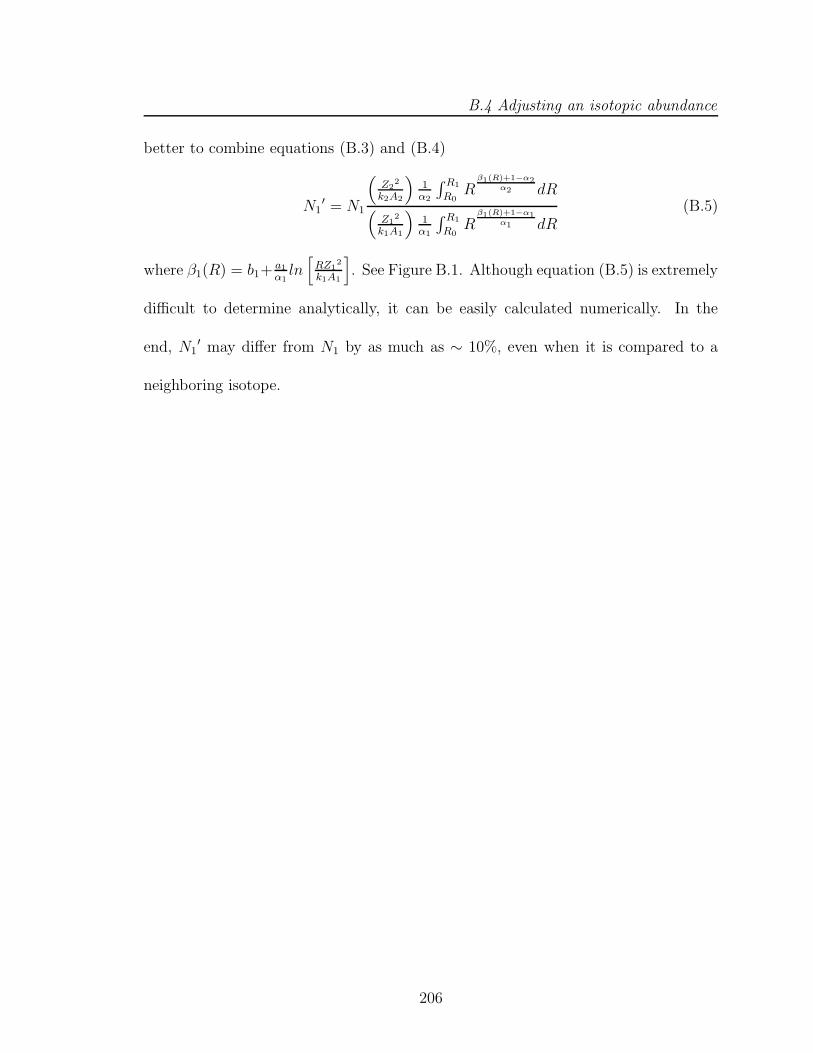
B.4 Adjusting an isotopic abundance
better to combine equations (B.3) and (B.4)
N1′ = N1
(
Z22
k2A2
)
1α2
∫ R1
R0R
β1(R)+1−α2α2 dR
(
Z12
k1A1
)
1α1
∫ R1
R0R
β1(R)+1−α1α1 dR
(B.5)
where β1(R) = b1+a1
α1ln
[
RZ12
k1A1
]
. See Figure B.1. Although equation (B.5) is extremely
difficult to determine analytically, it can be easily calculated numerically. In the
end, N1′ may differ from N1 by as much as ∼ 10%, even when it is compared to a
neighboring isotope.
206

B.4 Adjusting an isotopic abundance
α k(×10−3) α k(×10−3) α k(×10−3)10B 1.754 3.01 33S 1.694 4.06 50Ti 1.674 4.5511B 1.757 2.97 34S 1.696 4.03 49V 1.665 4.7712C 1.748 3.10 35Cl 1.689 4.17 50V 1.667 4.7413C 1.751 3.06 36Cl 1.691 4.13 51V 1.668 4.7114N 1.742 3.19 37Cl 1.693 4.10 50Cr 1.659 4.9215N 1.744 3.16 36Ar 1.683 4.32 51Cr 1.661 4.8916O 1.735 3.29 37Ar 1.684 4.29 52Cr 1.662 4.8517O 1.738 3.25 38Ar 1.686 4.25 53Cr 1.664 4.8118O 1.740 3.21 40Ar 1.690 4.17 54Cr 1.655 4.7819F 1.732 3.35 39K 1.680 4.39 53Mn 1.657 5.01
20Ne 1.724 3.48 40K 1.681 4.36 54Mn 1.658 4.9721Ne 1.726 3.44 41K 1.683 4.33 55Mn 1.659 4.9422Ne 1.728 3.41 40Ca 1.674 4.55 54Fe 1.651 5.1623Na 1.721 3.54 41Ca 1.675 4.51 55Fe 1.652 5.1324Mg 1.713 3.68 42Ca 1.677 4.46 56Fe 1.654 5.0925Mg 1.715 3.65 43Ca 1.679 4.42 57Fe 1.655 5.0626Mg 1.717 3.62 44Ca 1.680 4.40 58Fe 1.656 5.0326Al 1.707 3.79 45Sc 1.674 4.54 57Co 1.648 5.2527Al 1.710 3.75 44Ti 1.665 4.77 59Co 1.651 5.1828Si 1.703 3.89 46Ti 1.668 4.69 58Ni 1.643 5.4129Si 1.704 3.86 47Ti 1.670 4.66 60Ni 1.645 5.3430Si 1.706 3.82 48Ti 1.671 4.63 61Ni 1.647 5.3031P 1.700 3.95 49Ti 1.672 4.59 62Ni 1.648 5.2632S 1.693 4.10
Table B.1: Range-energy relation for selected isotopes. Fit parameters come fromthe relation R = kA
Z2Eα where A, Z, and E are the mass number, charge, and energy
per nucleon, respectively (Stone et al., 1998a). R is measured in g/cm2 of siliconafter the particle has traversed the material above the silicon stack detectors (thisamounts to a range of about 0.52 g/cm2 in silicon equivalent). This material wasapproximated as being composed of aluminum and polyethylene and stopping powerswere taken from (Janni, 1966). Energy loss in the silicon detector was calculatedbased on (Andersen and Ziegler, 1977; Wiedenbeck, 2003a).
207

Appendix C
Geometry Factor
C.1 The Monte-Carlo technique
In order for the CRIS instrument to accurately measure the charge Z, mass number
A, and energy per nucleon E, it is necesssary that incident particles stop inside the
telescope. This fact alone makes determining the geometry factor a non-trivial task.
For this analysis, a Monte-Carlo routine was developed with the same geometrical
cuts and dead layers for detectors 2 through 8, in all four telescopes, as specified in
§3.1.5. In this simulation, 105 “particles” were generated for each of 276 different
ranges in CRIS. The 276 ranges ran from 0.68 g/cm2 of silicon (the range to the
top of the E1 detector at θzenith = 0) to 16.8 g/cm2 (the range to the bottom of
detector E8 at θzenith = 50). The trajectory of each particle was given by two
coordinates, (R, θ0, φ0) and (R, θ1, φ1), such that 0 ≤ θ0 ≤ 90, 90 ≤ θ1 ≤ 180
and 0 ≤ φ0, φ1 ≤ 360. Each particle track was then aligned to intersect a sphere
with radius R = 46.0 cm (the radius of the active area for the E1 detector), centered
on the top surface of the E1 detector. In each case, the random values were uniformly
208

C.1 The Monte-Carlo technique
Figure C.1: An xz plot of simulated particles with θ < 30 that stop in the activearea in detector E8 in telescope 0. The dark areas delineate the inactive regions: theguard rings and dead layers in each Si detector.
distributed in cos θ and φ. The values were translated to (x0, y0, z0) and (x1, y1, z1)
in the normal way, and the angle of incidence for each particle was found
θzenith = tan−1
[
√
(x0 − x1)2 + (y0 − y1)2
z0 − z1
]
. (C.1)
Particles were then eliminated if their angles of incidence were greater than the spec-
ified amount (30 or 45 in this analysis), if they came to rest in detectors E1, E9
or any of the dead layers in detectors E2 through E8, or if at any point in their
trajectories, their radial distance from the center of the telescope exceeded 42.1 cm
for E2 through E7 or 46.0 cm for E8. Additionally, particles that stop in detector E8
are required to have trajectories that are within a radial distance of 46.0 cm when
projected to the surface of detector E9. Figure C.1 demonstrates this technique.
209

C.1 The Monte-Carlo technique
Figure C.2: The total geometry factor for the four CRIS telescopes, with a zenithacceptance angle of θ < 30 and θ < 45. Each curve corresponds to Gjk for aparticle stopping in an individual detector E2 through E8. The dotted line is thetotal geometry factor including all telescopes and detectors. The two internal axesindicate the corresponding energies for 16O and 56Fe nuclei.
The geometry factor, gijk, in the ith of telescopes 0 through 3, in the jth of detectors
E2 through E8, and in the kth of 276 ranges, can then be found
gijk = fijk · π · (πR2) (C.2)
where fijk is the fraction of the 105 particles that passed the cuts in the ith telescope,
in the jth detector, and in the kth range. The uncertainty on each determination of
gijk was calculated
σgijk=
√
fijk(1 − fijk)
N(C.3)
210

C.2 Determining the geometry factor and energy
for N = 105 particles.
The geometry factor for the sum of all telescopes in the j th detector in the kth
range was then defined
Gjk =
3∑
i=0
gijk (C.4)
with a corresponding uncertainty
σGjk=
√
√
√
√
3∑
i=0
(
σgijk
)2. (C.5)
The symbols plotted in Figure C.2 are the values of Gjk for the seven detectors (E2
to E8) at all 276 ranges in the instrument for zenith angles less than 30 and 45.
C.2 Determining the geometry factor and energy
We divide the CRIS data into isotopes that penetrate into a given detector in the
silicon stack. These events penetrate to a different depth in each detector depending
on the amount of energy that they have when they enter the instrument. For the
purposes of determining the differential intensity as discussed in §3.7, it is then left to
unify a given isotopic abundance measurement in a given range to one common energy
value and an appropriate Γj ≡∫
ΩAdE ≈ ∑276k=1GjkdEk (cm2 sr MeV/nucleon). We
use the “bowtie” method of Van Allen et al. (1974) to determine the appropriate
energy, Ej, and Γj for plotting the intensity (particles/cm2 sr s MeV/nucleon) of a
given isotope from the observed number of particles of that isotope stopping in the
jth detector.
211

C.2 Determining the geometry factor and energy
For particles stopping in the jth detector in CRIS, the differential spectrum for a
given isotope can be approximated very well as
dJ
dE= κjE
γ , (C.6)
where γ is observed to vary from ∼ 1.20 for 10B in detector E2 to ∼ −0.15 for 56Fe in
detector E8. Letting Nj be the observed number of particles of a given isotope per
unit time adjusted for spallation and SOFT efficiency stopping in the j th detector,
the differential intensity can then be expressed
dJ
dE=
Nj
Γj
. (C.7)
For a given γ, the observed number per unit time, Nj, can be expressed
Nj = κj
∫
G(E)EγdE ≡ κjIj(γ), (C.8)
where G(E) is the geometry factor derived in §C.1. The integral, Ij(γ), can be
approximated numerically as
Ij(γ) ≈276∑
k=1
[
1
2(Gj,k+1Ek
γ +GjkEkγ)(Ek+1 − Ek)
]
. (C.9)
For a given γ, there is a value of Γj corresponding to any Ej such that Equation
C.7 is satisfied. Combining Equations C.6, C.7 and C.8, we find the relationship
between Γj and Ej for a given γ to be
Ejγ =
Ij(γ)
Γj
. (C.10)
The exponent γ is not known a priori but the “bowtie” method notes that the Γj vs.
Ej lines defined by Equation C.10 for various values of γ all intersect at very nearly
212

C.2 Determining the geometry factor and energy
Figure C.3: Bowtie diagrams for 56Fe in detectors E2 through E8. The lines corre-spond to γ values of -0.2, 0.1, 0.4, 0.7, and 1.1. The appropriate values of Γ and E
for each detector can be found at the intersection points.
the same point. Using the Γj and Ej corresponding to that point permits us to plot
a point that lies on the differential intensity spectrum regardless of γ.
In this study, a set of γ were used ranging from -0.15 to 1.20 in increments of
0.05. For any two of these exponents, γm and γn, the intersection of the lines given
by Equation C.10 defines an E and Γ by
Ejmn =
[
Ij(γn)
Ij(γm)
]1
γn−γm
(C.11)
and
Γjmn =I(γm)
(Ejmn)γm. (C.12)
Figure C.3 shows the bowtie diagrams for 56Fe in all 7 detectors.
For a given isotope stopping in the jth detector, the value of Ej was defined as
the average of Equation C.11 for all m 6= n. An average Γj was then found with a
corresponding uncertainty, σΓj, equal to the standard deviation of Γjmn from Γj. The
213

C.2 Determining the geometry factor and energy
contribution of σΓjto the uncertainty in dJ
dEis small compared to other contributions
(i.e. uncertainties due to Gaussian fitting).
214

Appendix D
Isotopic Spectra
Figure D.1: Isotopic spectra (B to F), θ < 30. The filled circles are solar minimumdata; the open circles are for solar maximum. The lines are polynomial fits to thedata.
215

Figure D.2: Isotopic spectra (Ne to Ar), θ < 30. The filled circles are solar minimumdata; the open circles are for solar maximum. The lines are polynomial fits to thedata.
216

Figure D.3: Isotopic spectra (K to Cr), θ < 30. The filled circles are solar minimumdata; the open circles are for solar maximum. The lines are polynomial fits to thedata.
217

Figure D.4: Isotopic spectra (Mn to Ni), θ < 30. The filled circles are solarminimum data; the open circles are for solar maximum. The lines are polynomial fitsto the data.
218