Wavelet-Based Semantic Featuresfor Hyperspectral Signature Discrimination

Siwei Feng, Yuki Itoh, Mario Parente, Marco F. Duarte∗

Department of Electrical and Computer Engineering, University of Massachusetts, Amherst, MA, 01003, USA

Abstract

Hyperspectral signature classification is a quantitative analysis approach for hyperspectral imagery which

performs detection and classification of the constituent materials at the pixel level in the scene. The clas-

sification procedure can be operated directly on hyperspectral data or performed by using some features

extracted from the corresponding hyperspectral signatures containing information like the signature’s en-

ergy or shape. In this paper, we describe a technique that applies non-homogeneous hidden Markov chain

(NHMC) models to hyperspectral signature classification. The basic idea is to use statistical models (such

as NHMC) to characterize wavelet coefficients which capture the spectrum semantics (i.e., structural in-

formation) at multiple levels. Experimental results show that the approach based on NHMC models can

outperform existing approaches relevant in classification tasks.

Keywords: Classification, Hyperspectral Signatures, Semantics, Wavelet, Hidden Markov Model

1. Introduction

Hyperspectral remote sensors collect reflected image data simultaneously in hundreds of narrow, adjacent

spectral bands, forming a hyperspectral image cube consisting of a sequence of 2-D grayscale images where

each such image is obtained at a specific spectral band [1]. For each pixel, an almost continuous spectrum

curve can be derived [2], which can be referred to as a hyperspectral signature. The structure of such5

curve characterizes the on-ground (or near ground) constituent materials in a single remotely sensed pixel.

The four major applications in the hyperspectral image literature are target detection, change detection,

classification, and estimating the fraction of each material presented in the scene [2]. In this paper, we will

focus on the problem of hyperspectral signature classification.

The identification of ground materials from hyperspectral images often requires comparing the reflectance10

spectra of the image pixels, extracted endmembers, or ground cover exemplars to a training library of spectra

∗Corresponding authorEmail addresses: siwei@engin.umass.edu (Siwei Feng), yitoh@engin.umass.edu (Yuki Itoh), mparente@ecs.umass.edu

(Mario Parente), mduarte@ecs.umass.edu (Marco F. Duarte)

Preprint submitted to Elsevier September 2, 2016

obtained in the laboratory from well characterized samples. There is a rich literature on hyperspectral image

classification in the last decade, including schemes based on Scale-invariant Feature Transform (SIFT) [3],

parsimonious Gaussian process models [4], and dictionary learning for sparse representations [5, 6]. For

a more detailed survey on hyperspectral image classification, we refer readers to [7]. Nonetheless, classi-15

fication methods emphasizing matching to a spectral library and material identification have received less

attention [8–10]. On the one hand, many methods rely on nearest neighbor classification schemes based on

one of many possible spectral similarity measures to match the observed test spectra with training library

spectra. On the other hand, practitioners have designed feature extraction schemes that capture relevant

information, in conjunction with appropriate similarity metrics, in order to discriminate between different20

materials.

Classification methods based on spectral similarity measures can provide researchers with simple imple-

mentation and relatively small computational requirements; however, there is a tradeoff with the amount of

storage required for the training spectra as well as with the uneven performance of nearest neighbor methods.

High-dimensional hyperspectral data can often be shown to be well modeled by a lower dimensional struc-25

ture [11], where the lower dimensional structure is specific to each dataset. Therefore, in some cases taking

the whole spectrum into consideration brings a large amount of redundant information to practitioners, while

the role of relevant structural features is weakened. To ameliorate this issue, we will consider imparting

different weights for different wavelengths of the spectrum in the design of the classification features.

Practitioners recognize several structural features in the spectral curves of each material as “diagnostic”30

or characteristic of its chemical makeup, such as the position and shape of absorption bands. Several

approaches like the Tetracorder [12] have been proposed to encode such characteristics. However, such

techniques require the construction of ad-hoc rules to characterize instances of each material while new

rules must be created when spectral species which were not previously analyzed are added. Parente et al.

[13] proposed an approach using parametric models to represent the absorption features. However, it still35

requires the construction of specific rules to match observations to a training library.

In this paper, we consider the formulation of an information extraction process from hyperspectral sig-

natures via the use of mathematical models for hyperspectral signals. Our goal is to encode the signature’s

scientifically meaningful structural features into numerical features, which are referred to as semantic fea-

tures, without ad-hoc rules for the spectra of any material type. Our proposed method provides automated40

extraction of semantic information from the hyperspectral signature, in contrast with the aforementioned

diagnostic characteristics designed by hand by expert practitioners. Furthermore, no new rules should need

to be constructed when mineral species which were not analyzed before are added.

Mathematical signal models have been used to represent reflectance spectra. More specifically, mod-

els leveraging wavelet decompositions are of particular interest because they enable the representation of45

structural features at different scales. The wavelet transform is a popular tool in many signal processing

2

applications due to the capability of wavelet coefficients to characterize signal discontinuities at different

scales and offsets. As mentioned above, the semantic information utilized by researchers is heavily related to

the shape of reflectance spectra, which is succinctly represented in the magnitudes of its wavelet coefficients.

A coefficient with large magnitude generally indicates a rapid change in its support while a small wavelet50

coefficient generally implies a smooth region. Existing wavelet approaches are limited to filtering techniques

but do not extract features [8, 9].

In this paper, we apply hidden Markov models (HMMs) to the wavelet coefficients derived from the

observed hyperspectral signals so that the correlations between wavelet coefficients at adjacent scales can

be captured by the models. The HMMs allow us to identify significant vs. nonsignificant portions of the55

hyperspectral signatures with respect to the database used for training. The applications of HMMs for this

purpose is inspired by the hidden Markov tree (HMT) model proposed in [14]. As for the wavelet transform,

we use an undecimated wavelet transform (UWT) in order to obtain maximum flexibility on the set of scales

and offsets (spectral bands or wavelengths1) considered.

Our model for a spectrum encompassing N spectral bands takes the form of a collection of N non-60

homogeneous hidden Markov chains (NHMCs), each corresponding to a particular spectral band. Such a

model provides a map from each signal spectrum to a binary space that encodes the structural features at

different scales and wavelengths, effectively representing the semantic features that allow for the discrimina-

tion of spectra. To the best of our knowledge, the application of statistical wavelet models to the automatic

selection of semantically meaningful features in hyperspectral signatures has not been proposed previously.65

This paper is organized as follows. Section 2 introduces the mathematical background behind our

hyperspectral signature classification system and reviews relevant existing approaches for the hyperspectral

classification task. Section 3 provides an overview of the proposed feature extraction method, including

details about the choice of mother wavelet, statistical model training, and label computing; we also show

examples of the semantic information in hyperspectral signatures captured by the proposed features. Section70

4 describes our experimental test setup as well as the corresponding results. Finally, some conclusions are

provided in Section 5.

2. Background and Related Work

In this section, we begin by discussing several existing spectral matching approaches. Then, we review

the theoretical background for our proposed hyperspectral signature classification system, including wavelet75

analysis, hidden Markov chain models, and the Viterbi algorithm.

1We use these three equivalent terms interchangeably in the sequel.

3

2.1. Spectral Matching Measures

A direct comparison of spectral similarity measures taken on the observed hyperspectral signals is the

easiest and the most direct way to do spectral matching. Generally speaking, spectral similarity measures can

be combined with nearest neighbor classifiers. In this paper we use four commonly used spectral similarity80

measures. To present these measures, we use ri = (ri1, ri2, ..., riN )T and rj = (rj1, rj2, ..., rjN )T , to denote

the reflectance or radiance signatures of two hyperspectral image pixel vectors.

2.1.1. Spectral Angle Measure

The spectral angle measure (SAM) [15] between two reflectance spectra is defined as

SAM(ri, rj) = cos−1

(〈ri, rj〉√||ri||22||rj ||22

).

A smaller spectral angle indicates larger similarity between the spectra.

2.1.2. Euclidean Distance Measure85

The Euclidean distance measure (ED) [16] between two reflectance spectra is defined as ED(ri, rj) =

||ri−rj ||2. As with SAM, smaller ED implies larger similarity between two vectors. The ED measure takes

the intensity of two reflectance spectra into account, while the former is invariant to intensity.

2.1.3. Spectral Correlation Measure

The spectral correlation measure (SCM) [17] between two reflectance spectra is defined as

SCM(ri, rj) =

∑Nk=1(rik − r̄i)(rjk − r̄j)√∑N

k=1(rik − r̄i)2∑N

k=1(rjk − r̄j)2.

where r̄i is the mean of the values of all the elements in a reflectance spectrum vector ri. The SCM can90

take both positive or negative values; larger positive values are indicative of similarity between spectra.

2.1.4. Spectral Information Divergence Measure

The spectral information divergence measure (SID) [18] between two reflectance spectra is defined as

SID(ri, rj) = D(ri||rj)+D(rj ||ri), where D(ri||rj) is regarded as the relative entropy (or Kullback-Leibler

divergence) of rj with respect to ri, which is defined as

D(ri||rj) = −N∑

k=1

pik(log pjk − log pik).

Here pik = rik/∑N

k=1 rik corresponds to a normalized version of the spectrum ri at the kth spectral band,

which is interpreted in the relative entropy formulation as a probability distribution.

4

2.2. Wavelet Analysis95

The wavelet transform of a signal provides a multiscale analysis of a signal’s content which effectively

encodes in a compact fashion the locations and scales at which the signal structure is present [19]. To

date, several hyperspectral classification methods based on wavelet transform have been proposed. Most of

these classification approaches (e.g. [10, 20, 21]) employ a dyadic/decimated wavelet transform (DWT) as

the preprocessing step. Compared with UWT, the DWT provides a more concise representation because100

it minimizes the amount of redundancy in the coefficients. However, the tradeoff for such redundancy is

that UWT provides maximum flexibility on the choice of scales and offsets used in the multiscale analysis,

which is desired because it allows for a simple characterization of the spectrum structure at each individual

spectral band.

A one-dimensional real-valued UWT of an N -sample signal x ∈ RN is composed of wavelet coefficients

ws,n, each labeled by a scale s ∈ 1, ..., L and offset n ∈ 1, ..., N , where L 6 N . The coefficients are defined

using inner products as ws,n = 〈x, φs,n〉, where φs,n ∈ RN denotes a sampled version of the mother wavelet

function φ dilated to scale s and translated to offset n:

φs,n(λ) =1√sφ

(λ− ns

),

where λ is a scalar. Each coefficient ws,n, where s < L, has a child coefficient ws+1,n at scale s+1. Similarly,105

each coefficient ws,n at scale s > 1 has one parent ws−1,n at scale s − 1. Such a structure in the wavelet

coefficients enables the representation of fluctuations in a spectral signature by chains of large coefficients

appearing within the columns of the wavelet coefficient matrix W .

2.3. Advantages of Haar Wavelet

The Haar wavelet is the simplest possible compact wavelet which has the properties of square-like shape110

and discontinuity. These properties makes the Haar wavelet sensitive to a larger range of fluctuations than

other mother wavelets and provides it with a lower discriminative power. Thus, the Haar wavelet enables

the detection of both slow-varying fluctuations and sudden changes in a signal [19], while not particularly

sensitive to small discontinuities (i.e., noise) on a signal, in effect averaging them out over the wavelet

support.115

Consider the example in Fig. 2.3, where the figure at the top represents an example hyperspectral

signature, while the figures in the middle and at the bottom show the undecimated wavelet coefficient

matrix of the spectrum under the Haar and Daubechies-4 wavelets, respectively. The middle figure in

Fig. 2.3 shows the capability of Haar wavelets to capture both rapid changes and gently sloping fluctuations

in the sample reflectance spectrum. Similarly, the bottom figure shows that the Daubechies-4 wavelet is120

sensitive to compact and drastic discontinuities (i.e., higher order fluctuations that are often due to noise).

Thus, the Daubechies-4 wavelet does not provide a good match to semantic information extraction for this

5

Figure 1: Top: an example of normalized mineral reflectance (Garnet). Middle: corresponding UWT coefficient matrix (9-level

wavelet decomposition) using a Haar wavelet. Bottom: corresponding UWT coefficient matrix using a Daubechies-4 wavelet.

example reflectance spectrum. Intuitively, these issues will also be present for other higher-order wavelets,

which provide good analytical matches to functions with fast, high-order fluctuations.

In general, wavelet representations of spectral absorption bands are less emphasized under Haar wavelet125

than under other higher order wavelets. However, this drawback can be alleviated using discretization,

which will be described in the next subsection.

2.4. Statistical Modeling of Wavelet Coefficients

The pairwise statistics of DWT coefficients can be succinctly captured by a hidden Markov model [14].

The dyadic nature of DWT coefficients gives rise to a hidden Markov tree (HMT) model that characterizes130

the clustering and persistence properties of wavelet coefficients. The statistical model is constructed based

on the wavelet representation of spectra in a training library.

The statistical model is driven by the energy compaction property of the DWT. This property motivates

the use of a zero-mean Gaussian mixture model (GMM) with two Gaussian components. The first Gaussian

component features a high variance and characterizes the small number of “large” coefficients; thus, this state135

is labeled L. The second Gaussian component features a low variance and characterizes the large number

of “small” wavelet coefficients; thus, this state is labeled S. More precisely, the conditional probability

of a wavelet coefficient ws given the value of the state Ss can be written as p(ws|Ss = i) = N (0, σ2i,s),

where i = {S,L}. The state Ss ∈ {S,L} of a wavelet coefficient1 collects these labels, and is said to be

hidden because the label values are not explicitly observed. The two states are provided with likelihoods140

pSs(L) = p(Ss = L) and pSs

(S) = p(Ss = S) such that pSs(L) + pSs

(S) = 1. Consequently, the distribution

of the same wavelet coefficient can be written as p(ws) = pSs(L)N (0, σ2

L,s) + pSs(S)N (0, σ2

S,s).

1Since the same model is used for each chain of coefficients {S1,n, . . . , SL,n}, n = 1, . . . , N , we remove the index n from the

subscript for simplicity in this sequel whenever possible.

6

UWT coefficients exhibit a persistence property [22, 23], which states that chain of wavelet coefficients

at adjacent scales are consistently small or large with high probability. This property can be accurately

modeled by a non-homogeneous hidden Markov chain (NHMC) that links the states of wavelet coefficients

in the same offset. More specifically, the state Ss of a coefficient ws is only affected by the state Ss−1 of its

parent (if it exists) and by the value of its coefficient ws. The Markov chain in the NHMC is parameterized

by the likelihoods for the first state PS1(L) and PS1

(S), as well as the set of state transition matrices for the

different parent-child label pairs (Ss−1, Ss) for s > 1:

As =

pS→S,s pL→S,s

pS→L,s pL→L,s

, (1)

where pi→j,s := P (Ss = j|Ss−1 = i) for i, j ∈ {L,S}. The parameters for the NHMC

θ = {pS1(S), pS1(L), {As}Ls=2, {σS,s, σL,s}Ls=1}

(which include the probabilities for the first hidden states, the state transition matrices, and Gaussian

variances for each of the states) that maximize the likelihood of a set of observations can be obtained via

the expectation maximization (EM) algorithm [14, 24].145

2.5. Wavelet-based Spectral Matching

Many hyperspectral signature classification approaches have been proposed in the literature, with a

subset of them involving wavelet analysis [8–10, 25, 26]. In this paper, we review two approaches that are

particularly close in scope to our proposed method, which will be used for comparison in our numerical

experiments. Since our focus in this paper is on hyperspectral classification for individual pixels, we limit150

our comparison to methods that rely exclusively on the spectral of a given pixel or on features obtained from

the pixel’s spectra. More specifically, we do not compare to other methods that use additional information

(e.g. spatial information for a HSI) or that assume prior knowledge of the location of semantic information,

which is usually obtained from an expert practitioner.

First, Rivard et al. [8] propose a method based on the wavelet decomposition of the spectral data.155

The obtained wavelet coefficients are separated into two categories: low-scale components of power (LCP)

capturing mineral spectral features (corresponding to the first fine scales), and high-scale components of

power (HCP) containing the overall continuum (corresponding to coarser scales). The coefficients for the

LCP spectrum, which capture detailed structural features, are summed across scales at each spectral band.

This process can conceptually be described as a filtering approach, since the division into LCP and HCP160

effectively acts as a high-pass filter that preserves only the fine-scale detailed portion of the spectrum.

A second wavelet-based classification approach is proposed in [9]. This second approach applies an

UWT on the entire database. The set of wavelet coefficients for each separate wavelength is considered as

7

Figure 2: Examples of signed state labels as classification features. Top: Example normalized reflectance spectrum (Ilmenite).

Second: Corresponding 9-scale UWT coefficient matrix using a Haar wavelet. Third: Corresponding state label matrix from an

NHMC model using a zero-mean two-state GMM. Blue represents smooth regions, while red represents fluctuations. Bottom:

Corresponding features consisting of the state labels with added signs from the Haar wavelet coefficients. Green represents

smooth regions, while red represents decreasing fluctuations and blue represents increasing fluctuations.

a separate feature vector. Linear discriminant analysis (LDA) is performed on each one of these vectors for

dimensionality reduction purposes. The outputs are grouped into C classes, corresponding to the elements165

of interest, to train either a single multivariate Gaussian distribution or a GMM for each of the classes,

where a classification label or score is obtained for each wavelength. Finally, decision fusion is performed

among the wavelengths to obtain a single classification label for the spectrum. It is implicitly expected by

this method that the number of training samples for each one of the classes is sufficiently large so that the

class-specific Gaussian (mixture) models can be accurately constructed.170

3. NHMC-Based Feature Extraction and Classification

In this section, we introduce a feature extraction scheme for hyperspectral signatures that exploits a

Markov model for the signature’s wavelet coefficients. A wavelet analysis is used in an UWT to capture

information on the fluctuations of the spectra. The state labels extracted from the Markov model represent

the semantic information relevant for hyperspectral signal processing.175

3.1. Semantic Features from NHMC Labels

Once the model has been trained, the value of the states S = {Sl,n}l=1,...,L,n=1,...,N can be estimated

from the wavelet coefficients {wl,n}l=1,...,L,n=1,...,N of the spectrum x using a Viterbi algorithm [14, 27].

We collect the states into an L×N array S to obtain a semantic feature vector for the spectrum x: states

labeled as “large” describe statistically significant fluctuations in the spectrum at the given band and scale,180

8

while states labeled as “small” describe either the lack of fluctuation or lack of statistical significance of

the fluctuation over the training set. An example is shown in Figure 2, showing that large state labels

correspond to statistically meaningful fluctuations in the spectrum of a sample of ilmenite.

Figure 2 shows, however, that the state label itself does not encode information about the direction in

which the fluctuation occurs. Luckily, we find that this information can be easily extracted from the wavelet185

coefficient vector, when the Haar wavelet is used in the UWT [19]. Therefore, we choose to augment the

state array S by endowing each state label with the sign of the corresponding wavelet coefficient.

3.2. Multi-State Hidden Markov Chain Model

In our system, we choose to use the NHMC model described in Section 2.4 applied to the UWT via the

Haar wavelet. We select the Haar wavelet due to its special shape, which allows for the magnitude of the190

wavelet coefficients to be proportional to the slope of the spectra across the wavelet’s support. Furthermore,

the signs of these coefficients are indicative of the slope orientation (increasing or decreasing for negative

and positive, respectively).

In contrast to the prior work of [14], the NHMC approach we use here features k-state GMMs, with

k > 2, to model each wavelet coefficient. Our simulations have shown that the NHMC model with k = 2195

provides state labels with an overly coarse distinction between fluctuations and flat regions, which often

neglects to capture the presence of absorption bands (in particular weak bands); such bands often do

provide discriminants between mineral classes, and the performance of classification improves with larger

values of k, as will be shown in the sequel.

We associate each wavelet coefficient ws with an unobserved hidden state Ss ∈ {0, 1, ..., k − 1}, where

the states have prior probabilities pi,s := p(Ss = i) for i = 0, 1, ..., k − 1. Here the state i = 0 represents

smooth regions of the spectral signature, in a fashion similar to the small (S) state for binary GMMs,

while i = 1, . . . , k − 1 represent a more finely grained set of states for spectral signature fluctuations,

similarly to the large (L) state in binary GMMs. All the weights should meet the condition∑k−1

i=0 pi,s = 1.

Each state is characterized by a zero-mean Gaussian distribution for the wavelet coefficient with variance

σ2i,s. The value of Ss determines which of the k components of the mixture model is used to generate the

probability distribution for the wavelet coefficient ws: p(ws|Ss = i) = N (0, σ2i,s). We can then infer that

p(ws) =∑k−1

i=0 pi,sp(ws|Ss = i). In analogy with the binary GMM case, we can also define a k×k transition

probability matrix

As =

p0→0,s p1→0,s · · · pk−1→0,s

p0→1,s p1→1,s · · · pk−1→1,s

......

. . ....

p0→k−1,s p1→k−1,s · · · pk−1→k−1,s

,

9

Figure 3: Comparison of label arrays obtained from several statistical models for wavelet coefficients. Top: example normalized

reflectance, same as in Fig. 2. Second: Corresponding state label matrix from a 2-state GMM NHMC model. Third:

Corresponding state label matrix from a 6-state GMM NHMC model. Bottom: Corresponding state label matrix from a MOG

NHMC model with k = 6.

where pi→j,s = p(Ss = j|Ss−1 = i). Note that the probabilities in the diagonal of As are expected to be200

larger than those in the off-diagonal elements due to the persistence property of wavelet transforms. Note

also that all state probabilities pi,s for s > 1 can be derived from the matrices {As}Ls=2 and {pi,1}k−1i=0 .

3.3. Additional Modifications to NHMC

Unfortunately, a large number of GMM states might also have negative influence in semantic modeling

due to spectral variability, i.e., to the diversity of reflectance values for different bands. More specifically,205

we see in our experiments that the maps from rates of fluctuation to the k available state labels may be

significantly different for wavelet coefficients corresponding to neighboring bands. Although we observe that

the lowest variance state is consistently assigned to bands without statistically significant fluctuations, the

assignment of k-ary labels to fluctuations at different bands is not nearly as uniform, making the evaluation

of the spectral signature from the semantic features more difficult.210

Figure 3 provides an example comparison between labels obtained from the k-state GMM NHMC and the

MOG-NHMC; the figure highlights the variability obtained when k labels are used in the feature, reducing

its semantic significance, while MOG-NHMC retains semantic significance.

3.4. Illustration of Extracted Semantic Information

We have observed four distinct behaviors of hyperspectral signatures that are captured by the MOG-215

NHMC semantic features proposed above: (i) the direction of fluctuation in the reflectance spectra, which

is captured in the state label values; (ii) the width of the fluctuation, which is captured by the width of

10

Figure 4: Semantic information extracted in some sample spectral curves based on MOG with 2 states. Top row: Sample

spectral curves with extracted semantic information. Bottom row: corresponding state label array.

a sequence of matching labels through neighboring wavelengths; (iii) the slope of the fluctuation, which is

captured by the number of matching state values through the scales at the given spectral band; and (iv)

the locations of the absorption bands, which are captured by the band indices at which the feature switch220

from -1 to 1 or vice-versa. Figure 4 illustrates these four types of captured information in several example

reflectance spectra. First, we transform the state array S into a vector Sv by collecting the most prevalent

state for each band (i.e., the state that appears most often in each column of S). We show four example

reflectance spectra that are colored according to the state vector Sv (green, red, and blue for 0, +1, and

−1, respectively). The bands for which Sv fluctuates from 1 to -1 are labeled to identify the location of225

absorption minima. This representation can be considered a summary of the semantic information in the

spectra, equivalent to renditions such as the ones used by practitioners for automatic mineral identification.

The difference is that the semantic features in the NHMC approach are extracted directly from the data

and not defined a priori by an expert.

3.5. NHMC Classification Summary230

We provide an overview of the NHMC-based hyperspectral classification system in Fig. 5. The system

consists of two modules: an NHMC model training module and a classification module. The training stage

uses a training library of spectra containing samples from the classes of interest to train the NHMC model,

which is then used to compute state estimates for each of the training spectra using a Viterbi Algorithm.

The state arrays obtained from the NHMC model will then be used as classification features coupled with235

a classification scheme, e.g., nearest-neighbor (NN) or support vector machine (SVM) classification. The

testing module considers a spectrum under test and computes the state estimates under the trained NHMC

model using the parameters obtained during training. The module then applies the classification scheme

11

Figure 5: NHMC classification overview. Top: The classifier is trained from a set of training spectra; we compute UWT

coefficients for each spectrum, and feed the wavelet coefficient vectors to an NHMC training module that outputs the model

parameters and state label arrays for each of the training spectra, to be used as semantic features. Bottom: The classifier

considers a test spectrum, obtains its UWT coefficients, and extracts a state array from the aforementioned NHMC model to

use as semantic features. A nearest-neighbors search returns the most similar state array among the training data, as well as

the class label for the corresponding spectrum.

used during training to provide a label for the spectrum being tested.

4. Classification Experiments and Result Analysis on Synthetic Data240

In this section, we present multiple experimental results that assess the performance of the proposed

features in hyperspectral signature classification. We also study the effect of NHMC parameter selections

on the classification performance from the corresponding extracted features.

4.1. Study Data and Performance Evaluation

Our simulations use the RELAB spectral database with 26 mineral reflectance spectrum classes. To245

select a uniform range of wavelength for all spectra used, we focus on the spectral region 0.35 µm to 2.6 µm

corresponding to most of the visible and near-infrared region of the electromagnetic spectrum. The spectral

sampling step is 5 nm. The classes selected exhibit each a different number of measured spectra; therefore,

in order to avoid possible estimation biases in the NHMC and classifier training, we generate new samples

for each class by applying the Hapke mixing model [28] to existing samples with randomly selected mixture250

weights in order to increase the number of samples for each class to match the largest available (65). The

resulting dataset contains 1690 reflectance spectra that are normalized as well to remove the effect of varying

illumination conditions in classification.

12

We compare the proposed NHMC models: the different instances of the model we test use k = 2 to 10

classes, with and without MOG conversion and wavelet coefficient sign augmentation. Our training/testing255

datasets are obtained by a random 80%/20% partition for training and testing uniformly for each class

selected. Unfortunately, we observe that the classes in the resulting dataset are almost perfectly well

separated, making it difficult to differentiate between the proposed models in terms of performance as they

are near perfect for all. We therefore consider a more difficult problem that aims at identifying dominant

elements in material mixtures in a hyperspectral image where the pixels correspond to the testing sample260

described earlier under a randomized 2-D assignment to pixels. The mixtures are introduced to mimic

an image formation process that includes spatial blurring with a 3 × 3 Gaussian kernel, with the center

pixel corresponding to the dominant material and defining the sought label. The difficulty of the resulting

classification process is controlled in terms of the variance of the Gaussian blurring kernel, and is measured

in terms of the dominant material percentage (DMP), i.e., the weight of the center pixel in the blurring265

kernel. In our experiment, we vary the DMP from 70% to 100% with a step of 5%.

4.2. Feature Comparison

For this study, classification performance is evaluated by using NN and SVM classification accuracies.

For the NN classifier, three distance metrics are employed: `1 distance, Euclidean (`2) distance, and cosine

similarity measure. For the SVM classifier, we use radial basis function (RBF) as the kernel and perform a270

grid search for the corresponding parameter values (cost and Gaussian variance) that provide best perfor-

mance for each NHMC model. Both the NHMC model (if applicable) and the classifier (NN or SVM) are

trained using the aforementioned training set, and the performance is measured on the aforementioned test

set.

Figure 6 shows the classification rates for different NHMC models under different dominant material275

percentages using the aforementioned NN and SVM classifiers. Additionally, the figure also includes the

classification accuracies of the related approaches described in Section 2.5. In the figure, different classifica-

tion features are identified as follows: “Rivard” denotes the approach proposed in [8];2 “Wavelet Coefficient”

denotes the classification scheme of using wavelet coefficients as classification features; “Spectral Similarity”

denotes spectral similarity matching classification scheme (i.e., the spectra themselves are the input to each280

NN classifier); “GMM” denotes an NHMC featuring Gaussian mixture models; “MOG” denotes an NHMC

featuring mixtures of Gaussians; and “GMM+Sign” and “MOG+Sign” denotes the previous two approaches

where Haar wavelet coefficient signs being added to state labels. Our NHMC tests involve NHMC models

containing different numbers of mixed Gaussian components; Fig. 6 shows the highest performance among

all tested values for the number of mixed Gaussian components.285

2Note that “Rivard” only appears in the bottom left figure of Fig. 6 because it is defined specifically in terms of a NN

classifier with cosine distance [8].

13

Figure 6: Classification rates of different NHMC modeling approaches and other relative classification approaches under different

dominant material percentages. Top left: NN classifiers with `1 distance; top right: NN classifier with Euclidean distance;

bottom left: NN classifier with cosine similarity; bottom right: SVM classifier. For NHMC models, the highest classification

rate among the models tested is listed for each DMP value.

We highlight some features of the obtained results:

• In most cases, the use of signs in the NHMC features improves performance with respect to their

original counterparts.

• In the NN classifiers, GMM performs better than MOG for lower DMPs, which are more challenging

settings, while MOG with additional signs outperforms GMM for DMPs closer to 100%. Nonetheless,290

in most cases MOG without wavelet coefficient signs provides the worst performance.

• While the performance of NHMC methods with SVM classifiers is higher than that obtained with NN

classifiers, they are outperformed by the wavelet coefficient approach. We conjecture that this is due

to the discrete nature of NHMC labels, which are not as easily leveraged in the SVM’s search for a

separation boundary from support vectors.295

14

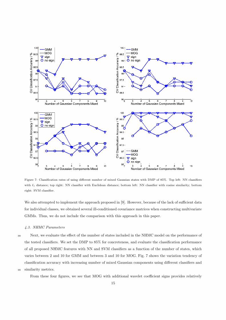
Figure 7: Classification rates of using different number of mixed Gaussian states with DMP of 85%. Top left: NN classifiers

with `1 distance; top right: NN classifier with Euclidean distance; bottom left: NN classifier with cosine similarity; bottom

right: SVM classifier.

We also attempted to implement the approach proposed in [9]. However, because of the lack of sufficient data

for individual classes, we obtained several ill-conditioned covariance matrices when constructing multivariate

GMMs. Thus, we do not include the comparison with this approach in this paper.

4.3. NHMC Parameters

Next, we evaluate the effect of the number of states included in the NHMC model on the performance of300

the tested classifiers. We set the DMP to 85% for concreteness, and evaluate the classification performance

of all proposed NHMC features with NN and SVM classifiers as a function of the number of states, which

varies between 2 and 10 for GMM and between 3 and 10 for MOG. Fig. 7 shows the variation tendency of

classification accuracy with increasing number of mixed Gaussian components using different classifiers and

similarity metrics.305

From these four figures, we see that MOG with additional wavelet coefficient signs provides relatively

15

consistent performance compared with other NHMC-based models. Additionally, in terms of classification

accuracy, the two model configurations using MOG provide two performance extremes: by adding wavelet

coefficient signs we obtain the highest classification performance, while MOG without signs provides the

lowest one. As mentioned earlier, MOG combines the simplicity of a binary-state GMM and the spectral310

fluctuation characterization capability of a multistate GMM. In that case, if we do not consider the signs

of the wavelet coefficient, spectra that have approximately matching locations for their fluctuations while

exhibiting differing magnitudes and orientations will be matched to similar MOG label vectors. The reason

is that a binary-state GMM form could assign the same state labels to several fluctuations of different levels

and orientations. However, if Haar wavelet coefficient signs are added, the state labels better reflect the315

spectral fluctuation orientation information.

5. Conclusion

In this paper, we proposed the design of a feature extraction scheme for hyperspectral signatures that

preserves the semantic information used by practitioners in signature discrimination (i.e., location of distin-

guishing fluctuations and discontinuities). Our approach is automated thanks to the use of statistical models320

for wavelet transform coefficients, which succinctly capture the location and magnitude of fluctuations in

the spectra observed. Furthermore, the statistical model also enables a segmentation of the spectra into

informative and non-informative portions. The success of statistical modeling is mostly dependent on the

availability of a large-scale database for training containing representative examples of the spectra that are

observed by the sensing system.325

We also tested the quality of the preservation of semantic information in our proposed features by using a

simple example hyperspectral classification system based on nearest neighbor search. We also compared our

feature extraction method with three existing feature extraction approaches for classification; the first ap-

proach is spectral matching, which performs classification directly on the hyperspectral signature; the second

approach performs classification directly on wavelet coefficients, and the third approach computes features330

as the sum of wavelet coefficients of certain scales. We showed that the performance of our proposed features

meets or exceeds that of baselines relying on spectral matching and wavelet coefficient representations, in

particular for high DMP.

While the performance of each method we tested decreases as the DMP is reduced, the reduction is

stronger for the MOG and GMM methods in comparison with some of their counterparts (in particular, to335

the case where NN with cosine similarity is applied directly on the spectra). We believe that this effect is due

to the additional difficulty of modeling signal classes of increased variability (as the DMP decreases) using

the extracted binary features. Nonetheless, we note that even with this handicap the performance of the

best combinations of NHMC features and NN classifiers exceeds the performance of the comparison baseline

16

methods when the DMP is sufficiently large. Furthermore, we believe that the size of the datasets we use340

here, while much larger than that of our previous results [29–31], may still be insufficient to fully exploit

the power of the statistical models leveraged here. Thus, further work will focus on expanding the size

of database and investigating additional modifications to the feature extraction scheme and the underlying

statistical models. As an example, NHMC models based on nonzero-mean GMM are an attractive alternative

to be pursued in the future, as in certain cases the histogram of wavelet coefficients cannot be accurately345

modeled by zero-mean Gaussian mixture models.

Acknowledgements

We thank Mr. Ping Fung for providing an efficient implementation of our NHMC training code that

largely decreased the time of running experiments.

Portions of this work have been presented at the IEEE Workshop on Hyperspectral Image and Signal350

Proc.: Evolution in Remote Sensing (WHISPERS) [29], the Allerton Conference on Communication, Control,

and Computing [30] the IEEE Int. Conf. Image Processing (ICIP) [31], and the IEEE Conference on

Computer Vision and Pattern Recognition Workshops (CVPRW) [24].

This work was supported by the National Science Foundation under grant number IIS-1319585.

This research utilizes spectra acquired with the NASA RELAB facility at Brown University.355

References

[1] P. K. Varshney, M. K. Arora, R. M. Rao, Signal processing for hyperspectral data, in: IEEE Int. Conf. Acoustics Speech

and Sig. Proc. Proceedings, Vol. 5, 2006, pp. V–V.

[2] G. Shaw, D. Manolakis, Signal processing for hyperspectral image exploitation, IEEE Sig. proc. magazine 19 (1) (2002)

12–16.360

[3] Y. Xu, K. Hu, Y. Tian, F. Peng, Classification of hyperspectral imagery using sift for spectral matching, in: IEEE Cong.

Image and Sig. Proc., Vol. 2, 2008, pp. 704–708.

[4] M. Fauvel, C. Bouveyron, S. Girard, Parsimonious gaussian process models for the classification of multivariate remote

sensing images, in: IEEE Int. Conf. Acoustics, Speech and Sig. Proc., 2014, pp. 2913–2916.

[5] P. Du, Z. Xue, J. Li, A. Plaza, Learning discriminative sparse representations for hyperspectral image classification, IEEE365

Jol. Selected Topics in Sig. Proc. 9 (6) (2015) 1089–1104.

[6] Z. He, L. Liu, R. Deng, Y. Shen, Low-rank group inspired dictionary learning for hyperspectral image classification, Sig.

Proc. 120 (2016) 209–221.

[7] G. Camps-Valls, D. Tuia, L. Bruzzone, J. A. Benediktsson, Advances in hyperspectral image classification: Earth moni-

toring with statistical learning methods, IEEE Sig. Proc. Magazine 31 (1) (2014) 45–54.370

[8] B. Rivard, J. Feng, A. Gallie, A. Sanchez-Azofeifa, Continuous wavelets for the improved use of spectral libraries and

hyperspectral data, Remote Sensing of Environment 112 (6) (2008) 2850–2862.

[9] S. Prasad, W. Li, J. E. Fowler, L. M. Bruce, Information fusion in the redundant-wavelet-transform domain for noise-robust

hyperspectral classification, IEEE Trans. Geoscience and Remote Sensing 50 (9) (2012) 3474–3486.

17

[10] X. Zhang, N. H. Younan, C. G. O’Hara, Wavelet domain statistical hyperspectral soil texture classification, IEEE Trans.375

geoscience and remote sensing 43 (3) (2005) 615–618.

[11] D. Landgrebe, Hyperspectral image data analysis, IEEE Sig. Proc. Magazine 19 (1) (2002) 17–28.

[12] R. N. Clark, G. A. Swayze, K. E. Livo, R. F. Kokaly, S. J. Sutley, J. B. Dalton, R. R. McDougal, C. A. Gent, Imaging

spectroscopy: Earth and planetary remote sensing with the usgs tetracorder and expert systems, Jol. Geophysical Research:

Planets 108 (E12).380

[13] M. Parente, H. D. Makarewicz, J. L. Bishop, Decomposition of mineral absorption bands using nonlinear least squares

curve fitting: Application to martian meteorites and crism data, Planetary and Space Science 59 (5) (2011) 423–442.

[14] M. S. Crouse, R. D. Nowak, R. G. Baraniuk, Wavelet-based statistical signal processing using hidden markov models,

IEEE Trans. sig. proc. 46 (4) (1998) 886–902.

[15] F. Kruse, A. Lefkoff, J. Boardman, K. Heidebrecht, A. Shapiro, P. Barloon, A. Goetz, The spectral image processing385

system (sips)—interactive visualization and analysis of imaging spectrometer data, Remote sensing of environment 44 (2)

(1993) 145–163.

[16] J. N. Sweet, The spectral similarity scale and its application to the classification of hyperspectral remote sensing data, in:

IEEE Workshops on Advances in Techniques for Analysis of Remotely Sensed Data, 2003, pp. 92–99.

[17] F. Van Der Meer, W. Bakker, Ccsm: Cross correlogram spectral matching, Int. Jol. Remote Sensing 18 (5) (1997) 1197–390

1201.

[18] C.-I. Chang, An information-theoretic approach to spectral variability, similarity, and discrimination for hyperspectral

image analysis, IEEE Trans. info. theory 46 (5) (2000) 1927–1932.

[19] S. Mallat, A wavelet tour of signal processing, Academic press, 1999.

[20] K. Masood, Hyperspectral imaging with wavelet transform for classification of colon tissue biopsy samples, in: Proc. SPIE395

7073, Applications of Digital Image Processing XXXI, Vol. 7073, 2008.

[21] T. West, S. Prasad, L. M. Bruce, Multiclassifiers and decision fusion in the wavelet domain for exploitation of hyperspectral

data, in: IEEE Int. Geoscience and Remote Sensing Symposium, 2007, pp. 4850–4853.

[22] S. Mallat, W. L. Hwang, Singularity detection and processing with wavelets, IEEE trans.info. theory 38 (2) (1992) 617–643.

[23] S. Mallat, S. Zhong, Characterization of signals from multiscale edges, IEEE Trans. Pattern Analysis and Machine Intel-400

ligence 14 (7) (1992) 710–732.

[24] S. Feng, M. F. Duarte, M. Parente, Universality of wavelet-based non-homogeneous hidden markov chain model features

for hyperspectral signatures, in: Proceedings of the IEEE Conf. Comp. Vis. and Patt. Recognition Workshops (CVPRW),

2015, pp. 19–27.

[25] Y. Qian, M. Ye, J. Zhou, Hyperspectral image classification based on structured sparse logistic regression and three-405

dimensional wavelet texture features, IEEE Trans. Geoscience and Remote Sensing 51 (4) (2013) 2276–2291.

[26] L. Shen, S. Jia, Three-dimensional gabor wavelets for pixel-based hyperspectral imagery classification, IEEE Trans. Geo-

science and Remote Sensing 49 (12) (2011) 5039–5046.

[27] L. R. Rabiner, A tutorial on hidden markov models and selected applications in speech recognition, Proc. the IEEE 77 (2)

(1989) 257–286.410

[28] B. Hapke, Theory of reflectance and emittance spectroscopy, Cambridge University Press, 2012.

[29] M. Parente, M. F. Duarte, A new semantic wavelet-based spectral representation, in: IEEE Workshop on Hyperspectral

Image and Signal Proc.: Evolution in Remote Sensing (WHISPERS), Gainesville, FL, 2013.

[30] M. F. Duarte, M. Parente, Non-homogeneous hidden markov chain models for wavelet-based hyperspectral image process-

ing, in: 51st Annual Allerton Conference on Communication, Control, and Computing (Allerton), 2013, pp. 154–159.415

[31] S. Feng, Y. Itoh, M. Parente, M. F. Duarte, Tailoring non-homogeneous markov chain wavelet models for hyperspectral

signature classification, in: IEEE Int. Conf. Image Proc. (ICIP), 2014, pp. 5167–5171.

18