Introduction to Hyperspectral Image Analysis

Peg Shippert, Ph.D. Earth Science Applications Specialist

Research Systems, Inc.

Background

The most significant recent breakthrough in remote sensing has been the development ofhyperspectral sensors and software to analyze the resulting image data. Fifteen years agoonly spectral remote sensing experts had access to hyperspectral images or software toolsto take advantage of such images. Over the past decade hyperspectral image analysis hasmatured into one of the most powerful and fastest growing technologies in the field ofremote sensing.

The “hyper” in hyperspectral means “over” as in “too many” and refers to the largenumber of measured wavelength bands. Hyperspectral images are spectrallyoverdetermined, which means that they provide ample spectral information to identifyand distinguish spectrally unique materials. Hyperspectral imagery provides the potentialfor more accurate and detailed information extraction than possible with any other type ofremotely sensed data.

This paper will review some relevant spectral concepts, discuss the definition ofhyperspectral versus multispectral, review some recent applications of hyperspectralimage analysis, and summarize image-processing techniques commonly applied tohyperspectral imagery.

Spectral Image Basics

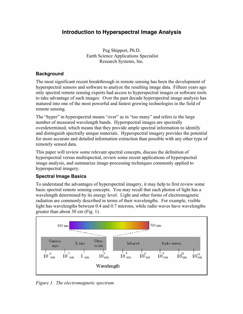
To understand the advantages of hyperspectral imagery, it may help to first review somebasic spectral remote sensing concepts. You may recall that each photon of light has awavelength determined by its energy level. Light and other forms of electromagneticradiation are commonly described in terms of their wavelengths. For example, visiblelight has wavelengths between 0.4 and 0.7 microns, while radio waves have wavelengthsgreater than about 30 cm (Fig. 1).

Figure 1. The electromagnetic spectrum

Reflectance is the percentage of the light hitting a material that is then reflected by thatmaterial (as opposed to being absorbed or transmitted). A reflectance spectrum showsthe reflectance of a material measured across a range of wavelengths (Fig. 2). Somematerials will reflect certain wavelengths of light, while other materials will absorb thesame wavelengths. These patterns of reflectance and absorption across wavelengths canuniquely identify certain materials.

Figure 2. Reflectance spectra measured by laboratory spectrometers for three materials:a green bay laurel leaf, the mineral talc, and a silty loam soil.

Field and laboratory spectrometers usually measure reflectance at many narrow, closelyspaced wavelength bands, so that the resulting spectra appear to be continuous curves(Fig. 2). When a spectrometer is used in an imaging sensor, the resulting images record areflectance spectrum for each pixel in the image (Fig. 3).

Figure 3. The concept of hyperspectral imagery. Image measurements are made atmany narrow contiguous wavelength bands, resulting in a complete spectrum for eachpixel.

Hyperspectral Data

Most multispectral imagers (e.g., Landsat, SPOT, AVHRR) measure radiation reflectedfrom a surface at a few wide, separated wavelength bands (Fig. 4). Most hyperspectralimagers (Table 1), on the other hand, measure reflected radiation at a series of narrowand contiguous wavelength bands. When we look at a spectrum for one pixel in ahyperspectral image, it looks very much like a spectrum that would be measured in aspectroscopy laboratory (Fig. 5). This type of detailed pixel spectrum can provide muchmore information about the surface than a multispectral pixel spectrum.

Figure 4. Reflectance spectra of the three materials in Figure 2 as they would appear tothe multispectral Landsat 7 ETM sensor.

Figure 5. Reflectance spectra of the three materials in Figure 2 as they would appear tothe hyperspectral AVIRIS sensor. The gaps in the spectra are wavelength ranges atwhich the atmosphere absorbs so much light that no reliable signal is received from thesurface.

Although most hyperspectral sensors measure hundreds of wavelengths, it is not thenumber of measured wavelengths that defines a sensor as hyperspectral. Rather it is thenarrowness and contiguous nature of the measurements. For example, a sensor thatmeasured only 20 bands could be considered hyperspectral if those bands werecontiguous and, say, 10 nm wide. If a sensor measured 20 wavelength bands that were,say, 100 nm wide, or that were separated by non-measured wavelength ranges, the sensorwould no longer be considered hyperspectral.

Standard multispectral image classification techniques were generally developed toclassify multispectral images into broad categories. Hyperspectral imagery provides anopportunity for more detailed image analysis. For example, using hyperspectral data,spectrally similar materials can be distinguished, and sub-pixel scale information can beextracted. To fulfill this potential, new image processing techniques have beendeveloped.

Most past and current hyperspectral sensors have been airborne (Table 1), with tworecent exceptions: NASA’s Hyperion sensor on the EO-1 satellite, and the U.S. AirForce Research Lab’s FTHSI sensor on the MightySat II satellite. Several new space-based hyperspectral sensors have been proposed recently (Table 2). Unlike airborne

sensors, space-based sensors are able to provide near global coverage repeated at regularintervals. Therefore, the amount of hyperspectral imagery available should increasesignificantly in the near future as new satellite-based sensors are successfully launched.

Table 1. Current and Recent Hyperspectral Sensors and Data Providers

SatelliteSensors

Manufacturer Number of Bands Spectral Range

FTHSI onMightySat II

Air Force ResearchLab

www.vs.afrl.af.mil/TechProgs/MightySatII

256 0.35 to 1.05 mm

Hyperion on EO-1

NASA Goddard SpaceFlight Center

eo1.gsfc.nasa.gov

220 0.4 to 2.5 mm

AirborneSensors

Manufacturer Number of Bands Spectral Range

AVIRIS(Airborne VisibleInfrared Imaging

Spectrometer)

NASA Jet PropulsionLab

makalu.jpl.nasa.gov/

224 0.4 to 2.5 mm

HYDICE(HyperspectralDigital Imagery

CollectionExperiment)

Naval Research Lab 210 0.4 to 2.5 mm

PROBE-1 Earth Search SciencesInc.

www.earthsearch.com

128 0.4 to 2.5 mm

casi(CompactAirborne

SpectrographicImager)

ITRES ResearchLimited

www.itres.com

up to 228 0.4 to 1.0 mm

HyMap Integrated Spectronics

www.intspec.com

100 to 200 Visible to thermalinfrared

EPS-H(Environmental

ProtectionSystem)

GER Corporation

www.ger.com

VIS/NIR (76), SWIR1 (32),SWIR2 (32), TIR (12)

VIS/NIR(.43 to 1.05 mm),

SWIR1(1.5 to 1.8 mm),

SWIR2(2.0 to 2.5 mm),

and TIR

(8 to 12.5 mm)

DAIS 7915(Digital Airborne

ImagingSpectrometer)

GER Corporation VIS/NIR (32), SWIR1 (8),SWIR2 (32), MIR (1),

TIR (6)

VIS/NIR(0.43 to 1.05 mm),

SWIR1(1.5 to 1.8 mm),

SWIR2(2.0 to 2.5 mm),

MIR(3.0 to 5.0 mm),

and TIR(8.7 to 12.3 mm)

DAIS 21115(Digital Airborne

ImagingSpectrometer)

GER Corporation VIS/NIR (76), SWIR1 (64),SWIR2 (64), MIR (1),

TIR (6)

VIS/NIR(0.40 to 1.0 mm),

SWIR1(1.0 to 1.8 mm),

SWIR2(2.0 to 2.5 mm),

MIR(3.0 to 5.0 mm),

and TIR(8.0 to 12.0 mm)

AISA(AirborneImaging

Spectrometer)

Spectral Imagingwww.specim.fi

up to 288 0.43 to 1.0 mm

Table 2. Proposed Space-Based Hyperspectral Sensors

Satellite Sensor Sponsoring Agencies

ARIES-I ARIES-I Auspace Ltd

ACRES

Earth Resource Mapping Pty. Ltd.

Geoimage Pty. Ltd.

CSIRO

PROBA CHRIS European Space Agency

NEMO COIS Space Technology Development Corporation

Naval Research Laboratory

PRISM European Space Agency

Application of Hyperspectral Image Analysis

Hyperspectral imagery has been used to detect and map a wide variety of materialshaving characteristic reflectance spectra. For example, hyperspectral images have beenused by geologists for mineral mapping (Clark et al., 1992, 1995) and to detect soilproperties including moisture, organic content, and salinity (Ben-Dor, 2000). Vegetationscientists have successfully used hyperspectral imagery to identify vegetation species(Clark et al., 1995), study plant canopy chemistry (Aber and Martin, 1995), and detectvegetation stress (Merton, 1999). Military personnel have used hyperspectral imagery todetect military vehicles under partial vegetation canopy, and many other military targetdetection objectives.

Atmospheric Correction

When sunlight travels from the sun to the Earth’s surface and then to the sensor, theintervening atmosphere often scatters some light. Therefore, the light received at thesensor may be more or less than that due to reflectance from the surface alone.Atmospheric correction attempts to minimize these effects on image spectra.Atmospheric correction is traditionally considered to be indispensable before quantitativeimage analysis or change detection using multispectral or hyperspectral data.Sophisticated atmospheric correction algorithms have been developed to calculateconcentrations of atmospheric gases directly from the detailed spectral informationcontained in hyperspectral imagery, without additional data about atmosphericconditions. Two such algorithms, ACORN from Analytical Imaging and Geophysics andFLAASH from Research Systems, are available as plug-in modules to ENVI.

Spectral LibrariesSpectral libraries are collections of reflectance spectra measured from materials of knowncomposition, usually in the field or laboratory. Many investigators collect spectrallibraries for materials in their field sites as part of every project, to facilitate analysis ofmultispectral or hyperspectral imagery from those sites. Several high quality spectrallibraries are also publicly available (e.g., Clark et al., 1993; Grove et al., 1992; Elvidge,1990; Korb et al., 1996; Salisbury et al., 1991a; Salisbury et al., 1991b; Salisbury et al.,1994). An ENVI installation includes 27 spectral libraries for a wide variety of materialsranging from minerals and vegetation to manmade materials. Spectra from libraries canguide spectral classifications or define targets to use in spectral image analysis.

Classification and Target Identification in ENVI

There are many unique image analysis algorithms that have been developed to exploit theextensive information contained in hyperspectral imagery. Most of these algorithms alsoprovide accurate, although more limited, analyses of multispectral data. Spectral analysismethods usually compare pixel spectra with a reference spectrum (often called a target).Target spectra can be derived from a variety of sources, including spectral libraries,regions of interest within a spectral image, or individual pixels within a spectral image.The most commonly used hyperspectral/multispectral image analysis methods that areprovided by ENVI are described below.

Whole Pixel Methods

Whole pixel analysis methods attempt to determine whether one or more target materialsare abundant within each pixel in a multispectral or hyperspectral image on the basis ofthe spectral similarity between the pixel and target spectra. Whole-pixel scale toolsinclude standard supervised classifiers such as Minimum Distance or MaximumLikelihood (Richards and Jia, 1999), as well as tools developed specifically forhyperspectral imagery such as Spectral Angle Mapper and Spectral Feature Fitting.

Spectral Angle Mapper (SAM)

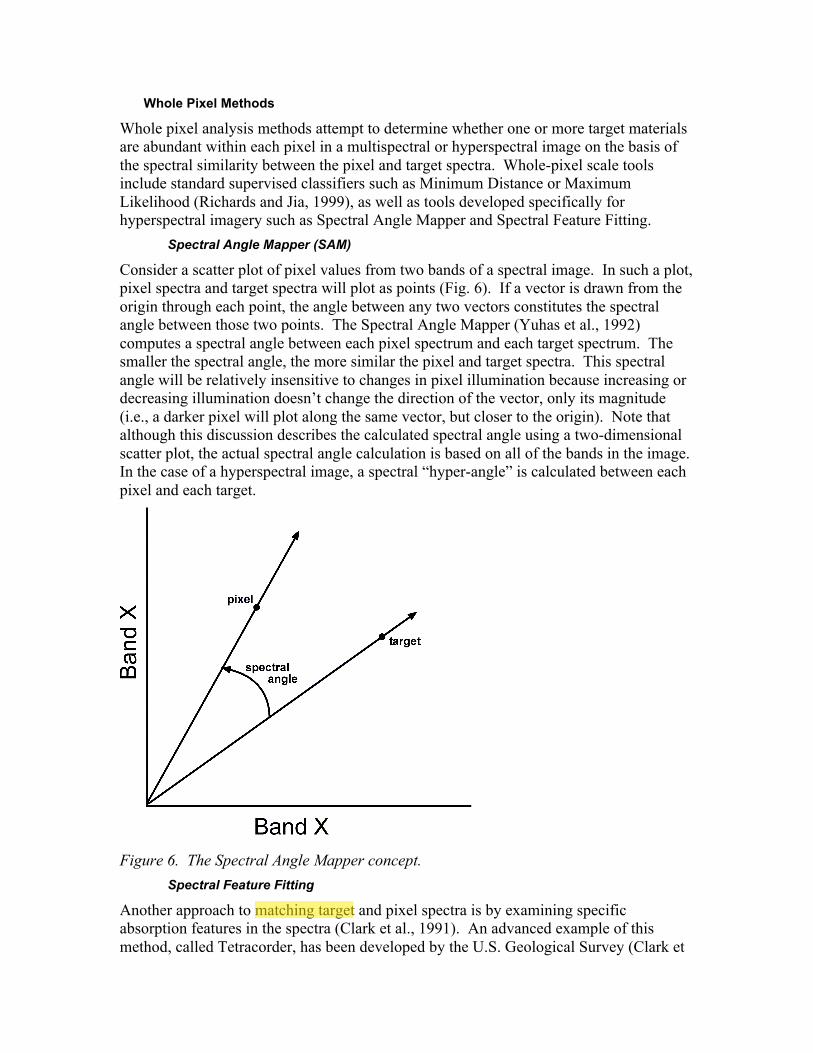
Consider a scatter plot of pixel values from two bands of a spectral image. In such a plot,pixel spectra and target spectra will plot as points (Fig. 6). If a vector is drawn from theorigin through each point, the angle between any two vectors constitutes the spectralangle between those two points. The Spectral Angle Mapper (Yuhas et al., 1992)computes a spectral angle between each pixel spectrum and each target spectrum. Thesmaller the spectral angle, the more similar the pixel and target spectra. This spectralangle will be relatively insensitive to changes in pixel illumination because increasing ordecreasing illumination doesn’t change the direction of the vector, only its magnitude(i.e., a darker pixel will plot along the same vector, but closer to the origin). Note thatalthough this discussion describes the calculated spectral angle using a two-dimensionalscatter plot, the actual spectral angle calculation is based on all of the bands in the image.In the case of a hyperspectral image, a spectral “hyper-angle” is calculated between eachpixel and each target.

Figure 6. The Spectral Angle Mapper concept.

Spectral Feature Fitting

Another approach to matching target and pixel spectra is by examining specificabsorption features in the spectra (Clark et al., 1991). An advanced example of thismethod, called Tetracorder, has been developed by the U.S. Geological Survey (Clark et

al., 2000). A relatively simple form of this method, called Spectral Feature Fitting, isavailable as part of ENVI. In Spectral Feature Fitting the user specifies a range ofwavelengths within which a unique absorption feature exists for the chosen target. Thepixel spectra are then compared to the target spectrum using two measurements: 1) thedepth of the feature in the pixel is compared to the depth of the feature in the target, and2) the shape of the feature in the pixel is compared to the shape of the feature in the target(using a least-squares technique).

Sub-Pixel MethodsSub-pixel analysis methods can be used to calculate the quantity of target materials ineach pixel of an image. Sub-pixel analysis can detect quantities of a target that are muchsmaller than the pixel size itself. In cases of good spectral contrast between a target andits background, sub-pixel analysis has detected targets covering as little as 1-3% of thepixel. Sub-pixel analysis methods include Complete Linear Spectral Unmixing, andMatched Filtering.

Complete Linear Spectral Unmixing

The set of spectrally unique surface materials existing within a scene are often referred toas the spectral endmembers for that scene. Linear Spectral Unmixing (Adams et al.,1986; Boardman, 1989) exploits the theory that the reflectance spectrum of any pixel isthe result of linear combinations of the spectra of all endmembers inside that pixel. Alinear combination in this context can be thought of as a weighted average, where eachendmember weight is directly proportional to the area the pixel containing thatendmember. If the spectra of all endmembers in the scene are known, then theirabundances within each pixel can be calculated from each pixel’s spectrum.

Unmixing simply solves a set of n linear equations for each pixel, where n is the numberof bands in the image. The unknown variables in these equations are the fractions of eachendmember in the pixel. To be able to solve the linear equations for the unknown pixelfractions it is necessary to have more equations than unknowns, which means that weneed more bands than endmember materials. With hyperspectral data this is almostalways true.

The results of Linear Spectral Unmixing include one abundance image for eachendmember. The pixel values in these images indicate the percentage of the pixel madeup of that endmember. For example, if a pixel in an abundance image for the endmemberquartz has a value of 0.90, then 90% of the area of the pixel contains quartz. An errorimage is also usually calculated to help evaluate the success of the unmixing analysis.

Matched Filtering

Matched Filtering (Boardman et al., 1995) is a type of unmixing in which only user-chosen targets are mapped. Unlike Complete Unmixing, we don’t need to find thespectra of all endmembers in the scene to get an accurate analysis (hence, this type ofanalysis is often called a ‘partial unmixing’ because the unmixing equations are onlypartially solved). Matched Filtering was originally developed to compute abundances oftargets that are relatively rare in the scene. If the target is not rare, special care must betaken when applying and interpreting Matched Filtering results.

Matched Filtering “filters” the input image for good matches to the chosen targetspectrum by maximizing the response of the target spectrum within the data andsuppressing the response of everything else (which is treated as a composite unknownbackground to the target). Like Complete Unmixing, a pixel value in the output image isproportional to the fraction of the pixel that contains the target material. Any pixel with avalue of 0 or less would be interpreted as background (i.e., none of the target is present).

One potential problem with Matched Filtering is that it is possible to end up with falsepositive results. One solution to this problem that is available in ENVI is to calculate anadditional measure called “infeasibility”. Infeasibility is based on both noise and imagestatistics and indicates the degree to which the Matched Filtering result is a feasiblemixture of the target and the background. Pixels with high infeasibilities are likely to befalse positives regardless of their matched filter value.

Summary

Hyperspectral sensors and analyses have provided more information from remotelysensed imagery than ever possible before. As new sensors provide more hyperspectralimagery and new image processing algorithms continue to be developed, hyperspectralimagery is positioned to become one of the most common research, exploration, andmonitoring technologies used in a wide variety of fields.

References

Aber, J. D., and Martin, M. E., 1995, High spectral resolution remote sensing of canopychemistry. In Summaries of the Fifth JPL Airborne Earth Science Workshop, JPLPublication 95-1, v. 1, pp. 1-4.

Adams, J. B., Smith, M. O., and Johnson, P.E., 1986, Spectral mixture modeling: A newanalysis of rock and soil types at the Viking Lander 1 site. Journal of GeophysicalResearch, vol. 91(B8), pp. 8090-8112.

Ben-Dor, E., Patin, K., Banin, A. and Karnieli, A., 2001, Mapping of several soilproperties using DAIS-7915 hyperspectral scanner data. A case study over clayeysoils in Israel. International Journal of Remote Sensing (in press).

Boardman, J. W., 1989, Inversion of imaging spectrometry data using singular valuedecomposition. Proceedings of the Twelfth Canadian Symposium on RemoteSensing, v. 4., pp. 2069-2072.

Boardman, J. W., Kruse, F. A., and Green, R. O., 1995, Mapping target signatures viapartial unmixing of AVIRIS data. In Summaries of the Fifth JPL Airborne EarthScience Workshop, JPL Publication 95-1, v. 1, pp. 23-26.

Clark, R. N., and Swayze, G. A., 1995, Mapping minerals, amorphous materials,environmental materials, vegetation, water, ice, and snow, and other materials:The USGS Tricorder Algorithm. In Summaries of the Fifth Annual JPL AirborneEarth Science Workshop, JPL Publication 95-1, v. 1, pp. 39 - 40.

Clark, R. N., Swayze, G. A., Gallagher, A., Gorelick, N., and Kruse, F. A., 1991,Mapping with imaging spectrometer data using the complete band shape least-squares algorithm simultaneously fit to multiple spectral features from multiple

materials. In Proceedings of the Third Airborne Visible/Infrared ImagingSpectrometer (AVIRIS) workshop, JPL Publication 91-28, pp. 2-3.

Clark, R. N., Swayze, G. A., and Gallagher, A., 1992, Mapping the mineralogy andlithology of Canyonlands, Utah with imaging spectrometer data and the multiplespectral feature mapping algorithm. In Summaries of the Third Annual JPLAirborne Geoscience Workshop, JPL Publication 92-14, v 1, pp. 11-13.

Clark, R. N., Swayze, G. A., Gallagher, A. J., King, T. V. V., and Calvin, W. M., 1993,The U. S. Geological Survey, Digital Spectral Library. Version 1: 0.2 to 3.0microns. U.S. Geological Survey Open File Report 93-592, 1340 pages.

Clark, R. N., Swayze, G. A., King, T. V. V., 2001, Imaging Spectroscopy: A Tool forEarth and Planetary System Science Remote Sensing with the USGS TetracorderAlgorithm, Journal of Geophysical Research (submitted).

Elvidge, C. D., 1990, Visible and infrared reflectance characteristics of dry plantmaterials. International Journal of Remote Sensing, v. 11(10), pp. 1775 - 1795.

Grove, C. I., Hook, S. J., and Paylor, E. D., 1992, Laboratory reflectance spectra for 160minerals 0.4 - 2.5 micrometers. JPL Publication 92-2.

King, R. N., Trude, V. V., Ager, C., and Swayze, G. A., 1995, Initial vegetation speciesand senescence/stress indicator mapping in the San Luis Valley, Colorado usingimaging spectrometer data. In Summaries of The Fifth Annual JPL AirborneEarth Science Workshop, vol. 1, p. 35-38.

Korb, A. R., Dybwad, P., Wadsworth, W., and Salisbury, J. W., 1996, Portable FTIRspectrometer for field measurements of radiance and emissivity. Applied Optics,v. 35, pp. 1679-1692.

Merton, R. N., 1999, Multi-temporal analysis of community scale vegetation stress withimaging spectroscopy. Ph.D. Thesis, Geography Department, University ofAuckland, New Zealand, 492p.

Richards, J.A., and Jia, X., 1999, Remote Sensing Digital Image Analysis, anIntroduction. Third Edition. Springer-Verlag: Berlin.

Salisbury, J. W., D'Aria, D. M., and Jarosevich, E., 1991a, Midinfrared (2.5-13.5micrometers) reflectance spectra of powdered stony meteorites. Icarus, v. 92, pp.280-297.

Salisbury, J. W., Wald, A., and D'Aria, D. M., 1994, Thermal-infrared remote sensingand Kirchhoff's law 1. Laboratory measurements. Journal of GeophysicalResearch, v. 99, pp. 11,897-11,911.

Salisbury, J. W., Walter, L. S., Vergo, N., and D'Aria, D. M., 1991b, Infrared (2.1- 25micrometers) Spectra of Minerals. Johns Hopkins University Press, 294 p.

Yuhas, R.H., Goetz, A. F. H., and Boardman, J. W., 1992, Discrimination among semi-arid landscape endmembers using the spectral angle mapper (SAM) algorithm. InSummaries of the Third Annual JPL Airborne Geoscience Workshop, JPLPublication 92-14, vol. 1, pp. 147-149.

AuthorPeg Shippert is the Earth Science Applications Specialist for Research Systems, Inc.(www.researchsystems.com), the makers of ENVI and IDL and a wholly ownedsubsidiary of Eastman Kodak. She has a Ph.D. in physical geography and more than 13years of experience analyzing multispectral and hyperspectral imagery for a wide varietyof applications.