an evaluation of hyperspectral and multispectral data for
TRANSCRIPT

AN EVALUATION OF HYPERSPECTRAL AND MULTISPECTRAL
DATA FOR MAPPING INVASIVE SPECIES IN AN AFRICAN
SAVANNA
Mahlatse Lucky Kganyago
214576229
A dissertation submitted to the College of Agriculture, Engineering and Science, in fulfilment
of the academic requirements for the degree of Master of Science in Geography and
Environmental Sciences
School of Agricultural, Earth and Environmental Sciences
University of KwaZulu-Natal,
Pietermaritzburg, South Africa
December 2015

i
DECLARATION
I, Mahlatse Lucky Kganyago, declare that:
The research reported in this document is my original work, unless indicated otherwise.
This dissertation has not been submitted for attainment of a degree or examination purposes at
another university.
This dissertation does not contain any data, graphics, and other information from other persons,
unless duly acknowledged.
This dissertation does not contain other persons’ writing, unless duly acknowledged as such. In
cases where written sources have been cited, their words have been paraphrased and general
information attributed to them has been referenced, and where exact words have been used, they
were placed inside quotation marks, referenced and italicized.
This dissertation does not contain text, graphics, and or tables directly copied and pasted from
the internet, unless otherwise sources were duly acknowledged within the content of this
dissertation.
This dissertation contains reproduced work from publications/manuscripts of which I am the first
author, as such my contribution was the greatest with co-authors providing guidance and such
publications have been duly referenced.
Signed:
Mahlatse Lucky Kganyago (214576229)
As the candidate’s supervisor/co-supervisor, I certify that the above declaration is true to the best
of my knowledge and have approved this dissertation for submission.
Signed:
Supervisor: Dr. John Odindi
Signed:
Co-supervisor: Dr. Paidamwoyo Mhangara
ii
PUBLICATIONS AND MANUSCRIPTS
The following manuscripts are under peer-review or being prepared for publication. I
substantially contributed to the study design, fieldwork, analysis, interpretation and discussion
of the results and the overall preparation of the manuscripts, hence I was the appropriate first
author in both manuscripts.
Kganyago, M., Odindi, J., Adjorlolo, C. & Mhangara, P. (Under Review). Determining optimal
spectral subset for discrimination of Parthenium hysterophorus: A hierarchical approach using
statistical filters and Support Vector Machine - Recursive Feature Elimination wrapper. ISPRS
Journal of Photogrammetry and Remote Sensing. [Chapter 2]
Kganyago, M., Odindi, J. Adjorlolo, C. & Mhangara, P. (In preparation). Evaluating the
Capability of Landsat 8 OLI and SPOT 6 for Discriminating Invasive Alien Species within the
Savanna Landscapes of KwaZulu-Natal, South Africa. Journal of Applied earth Observation and
Geo-information. [Chapter 3]
An oral presentation titled “Evaluating the Efficacy of Multispectral Remote Sensing for
Detecting and Estimating Patch Sizes of Parthenium Hysterophorus L. (Parthenium Weed) in
Kwazulu-Natal, South Africa” was presented by Kganyago, M. at 10th Biennial African
Association for Remote Sensing of the Environment (AARSE) Conference 2014, University of
Johannesburg, South Africa. [Chapter 3]
Signed:

iii
ABSTRACT
Invasive alien plant (IAP) species affects a range of ecosystem types in various regions of the
world. Therefore are now considered one of the main phenomena causing global change.
Invasive alien plants (IAP’s) cause considerable impacts on ecosystem processes and functions,
biodiversity, agriculture and human well-being. Parthenium hysterophorus is an IAP which is
widely spread across the globe. It is difficult to control and eradicate, and has detrimental impacts
on the natural environment and human health. However, there is no record of accurate and up-
to-date information on the distributions and extent of P. hysterophorus. This study evaluated the
capability of hyperspectral and multispectral data for mapping P. hysterophorus in northern
KwaZulu-Natal province, South Africa. First, the study sought to determine an optimal subset
of bands from canopy hyperspectral data for discrimination of P. hysterophorus from its co-
existing species. A novel hierarchical approach that integrates statistical filters and a wrapper
technique has been proposed to select optimal bands to solve the problem of high spectral
dimensionality and improve classification accuracy. A non-parametric algorithm, Support
Vector Machines (SVM) showed inferior classification accuracy, i.e. 76.19% and 78.57% when
using 20 best spectral bands from SVM – Recursive Feature Elimination (SVM-RFE) and entire
dataset (n = 1633), respectively. On the other hand, superior overall accuracy of 83.33% was
achieved when using ten spectral bands identified by the hierarchical approach. Next, SVM
classifier was adopted to evaluate the capability of multispectral data (i.e. Operational Land
Imager, OLI and SPOT 6) for determining the distribution and patch sizes of P. hysterophorus.
The results showed that SPOT 6 had a higher overall accuracy of 83.33% than OLI, i.e.76.39%.
While SPOT 6’s the higher spatial resolution was useful for better characterisation of the
distribution and patch sizes, the study found that the spectral configuration of OLI was more
important in identifying possible locations infested by P. hysterophorus. Overall, the study
demonstrated that fewer spectral bands selected by the proposed hierarchical approach have the
greatest potential for reliably discriminating IAP species using airborne and satellite
hyperspectral sensors. The study also demonstrated that the current information needs on IAP’s
can be addressed using accessible multispectral data, valuable for effective land management,
site specific weed management, and site prioritisation.

iv
DEDICATION
To my dear daughter, Oarona, you give me courage and strength to live each day.
To my dearly loved mother; Rebecca, my sisters; Lydia and Magdeline, my brothers; Joseph
(late), William and Thapelo, my nephews and my fiancée and best friend, Milly Mohlono, for
your motivations, laughter, love, and prayers that have kept me going.

v
ACKNOWLEDGEMENTS
Foremost, I thank God for granting me the ability to understand and to receive information from
his servants, for giving me the strength to carry on, for his patience and mercy, for preserving
my life, for providing me with great people to learn from and for his guidance.
I would like to express my sincere gratitude to the South African National Space Agency
(SANSA) for funding my studies and living expenses during my study period, for all the
opportunities to advance my competences and the exposure to conferences and forums to share
my work. I thank Dr. Paida Mhangara for his guidance, support, motivation and most of all, his
believe in me from the first day. I would like to thank Mr. Phila Sibandze, who assisted me to
adjust to the working environment, guided me towards achieving my personal, professional and
studying goals, and by the manner he carried his professional activities, inspired me to do the
same. I thank him for assistance during fieldwork, language editing and proof-reading of my
dissertation. I would also like to extend my sincere gratitude to all SANSA staff who in one way
or another contributed to my professional development, hence the completion of this study. I
would not have done it if it was not for your good wishes and support.
I would like to express my infinite appreciation and deepest gratitude to my supervisors, Dr.
John Odindi, Dr. Paida Mhangara and Dr. Clement Adjorlolo for their constant support,
invaluable critical comments and expert advice, wisdom, enthusiasm and determination to build
my scientific reasoning. Special thanks to Dr. Adjorlolo, who was diligently hands-on during the
fieldwork at Ndumo Game Reserve and shared his wide experience and knowledge in remote
sensing and ecology.
I would like to thank KZN Wildlife for their permission to conduct the study in Ndumo Game
Reserve. A Special thanks to Mr. Lucas Gumede for his assistance with the fieldwork and Mr.
Ian Rushworth for assisting in identifying the study area and facilitating the fieldwork. Last but
not least, I would like to thank my mother, who taught me to love, to laugh, to pray, to work
hard, to play and all other principles of life. I thank my dear daughter, Oarona and my fiancée,
Milly for being there for me always and giving me courage to continue living each day.

vi
Table of Contents
DECLARATION .......................................................................................................................... i
PUBLICATIONS AND MANUSCRIPTS .................................................................................. ii
ABSTRACT ................................................................................................................................ iii
DEDICATION ............................................................................................................................ iv
ACKNOWLEDGEMENTS ......................................................................................................... v
CHAPTER 1 ................................................................................................................................. 1
GENERAL INTRODUCTION .................................................................................................... 1
1.1. Background .................................................................................................................... 1
1.1.1. The potential of Remote Sensing for IAP species discrimination ......................... 3
1.1.2. Hyperspectral remote sensing of IAP species ........................................................ 4
1.1.3. Multispectral remote sensing of IAP species ......................................................... 5
1.1.4. Classification algorithms and vegetation indices for discriminating IAP species . 7
1.1.5. Challenges and opportunities for discrimination of P. hysterophorus ................... 8
1.2. Research problem .......................................................................................................... 9
1.3. Aim and Objectives ..................................................................................................... 10
1.3.1. Aim ....................................................................................................................... 10
1.3.2. Objectives ............................................................................................................. 10
1.4. Research questions ...................................................................................................... 10
1.5. Scope of the study ....................................................................................................... 11
1.6. Study area .................................................................................................................... 11
1.7. Chapter outline ............................................................................................................ 12
CHAPTER 2 ............................................................................................................................... 14
DETERMINING THE OPTIMAL SPECTRAL SUBSET FOR DISCRIMINATING
PARTHENIUM HYSTEROPHORUS ...................................................................................... 14
2.1. Introduction ................................................................................................................. 14
2.2. Materials and methods ................................................................................................. 16
2.2.1. Species description ............................................................................................... 16
2.2.2. Data collection...................................................................................................... 17
2.2.3. Pre-processing and analysis ................................................................................. 19

vii
2.2.4. SVM classification and validation ....................................................................... 21
2.3. Results ......................................................................................................................... 22
2.3.1. Kruskal-Wallis ANOVA ...................................................................................... 22
2.3.2. Inter-band correlation and AUC-ROC variable importance ................................ 24
2.3.3. SVM-RFE............................................................................................................. 25
2.3.4. SVM Classification and validation ...................................................................... 26
2.4. Discussions .................................................................................................................. 28
2.5. Conclusions ................................................................................................................. 32
CHAPTER 3 ............................................................................................................................... 34
EVALUATING THE CAPABILITY OF LANDSAT 8 OLI AND SPOT 6 FOR MAPPING
INVASIVE ALIEN SPECIES IN THE SAVANNA LANDSCAPES OF KWAZULU-NATAL.
.................................................................................................................................................... 34
3.1. Introduction ................................................................................................................. 34
3.2. Data and materials ....................................................................................................... 36
3.2.1. Data description.................................................................................................... 36
3.3. Methods ....................................................................................................................... 38
3.3.1. Pre-processing ...................................................................................................... 38
3.3.2. Support Vector Machines (SVM) Classification ................................................. 38
3.3.3. Distribution and patch sizes of P. hysterophorus ................................................. 39
3.3.4. Accuracy assessment and map comparisons ........................................................ 40
3.4. Results ......................................................................................................................... 41
3.4.1. Parameterisation of SVM classifier...................................................................... 41
3.4.2. SVM classification results .................................................................................... 41
3.4.3. Accuracy assessment and map comparisons ........................................................ 42
3.4.4. Distribution and patch sizes of P. hysterophorus ..................................................... 44
3.5. Discussions .................................................................................................................. 45
3.5.1. The capability of multispectral data for mapping P. hysterophorus .................... 45
3.5.2. Addressing information needs for optimising control mechanisms ..................... 48
3.6. Conclusions ................................................................................................................. 51
CHAPTER 4 ............................................................................................................................... 52
SYNTHESIS AND CONCLUSION .......................................................................................... 52

viii
4.1. Introduction ................................................................................................................. 52
4.2. Improving classification accuracy through feature subset selection and dimensionality
reduction ................................................................................................................................. 53
4.3. Optimal spectral bands for discrimination of P. hysterophorus .................................. 54
4.4. Reliable information for effective management of P. hysterophorus ......................... 57
4.5. Conclusions and Recommendations ............................................................................ 58
REFERENCES ........................................................................................................................... 60
APPENDICES ............................................................................................................................ 74

ix
List of Figures
Figure 1. Factors affecting reflectance properties in various regions of electromagnetic
spectrum and a comparison of contiguous spectral signature of P. hysterophorus (PH) and
discrete band positions of multispectral data (Landsat 8 OLI). ................................................... 4
Figure 2. Study area................................................................................................................... 12
Figure 3. Kruskal-Wallis ANOVA and post hoc Dunn’s test results for P. hysterophorus (PH)
and Acacia Trees (AT) (a); PH and Grass species (GS) (b) and PH and Other Plant Species
(OPS) (c). The frequency of occurrence of significant spectral bands (d), where PH can be
discriminated from all other co-existing species. ....................................................................... 23
Figure 4. Kendall's τ correlation analysis .................................................................................. 24
Figure 5. Spectral subset sizes evaluated by SVM-RFE on statistically filtered and entire
spectral datasets. ......................................................................................................................... 26
Figure 6. Differences in canopy and leaf structures of P. hysterophorus (a), Acacia Trees (b),
Grass Species (c) and Other Plant Species (d) ........................................................................... 30
Figure 7. P. hysterophorus infestations derived from Landsat 8 OLI (a) and SPOT 6 (b). ...... 42
Figure 8. Overall Quantity and Exchange difference for Landsat 8 (Left) and SPOT 6 (Right).
.................................................................................................................................................... 43
Figure 9. Receiver Operating Characteristic (ROC) curve variable importance for OLI and
SPOT 6. ...................................................................................................................................... 44
Figure 10. P. hysterophorus patch sizes calculated from OLI and SPOT 6.............................. 45
Figure 11. SPOT 6 patch sizes in communal croplands overlaid on aerial image acquired in
2009/10 and picture on the right represents the respective infested areas as seen in the field in
February 2014. ........................................................................................................................... 50
Figure 12. Canopy and leaf structures and spectral signatures of P. hysterophorus (PH), Acacia
Trees (AT), Grass species (GS) and Other plant species (OPS). ............................................... 54

x
List of Tables
Table 1. Potential multispectral data for mapping IAP species. .................................................. 7
Table 2. The number of plots and measurements per species ................................................... 19
Table 3. Number of significant wavelengths for each pair of classes separated by broad
spectral regions suggested by Fernandes et al. (2013). T denotes total number of input spectral
bands........................................................................................................................................... 23
Table 4. Selected spectral bands and their associated AUC-ROC importance. ........................ 25
Table 5. Confusion matrix for hierarchical approach ................................................................ 27
Table 6. Confusion matrix for entire spectral dataset ................................................................ 27
Table 7. Confusion matrix for a combination of 20 spectral bands ranked by SVM-RFE ....... 28
Table 8. Comparison of performance between the hierarchical approach, SVM-RFE and entire
spectral dataset. .......................................................................................................................... 32
Table 9. Landsat 8 OLI and SPOT 6 characteristics. ................................................................ 37
Table 10. Training and validation datasets for classifying P. hysterophorus........................... 38
Table 11. Confusion matrices for OLI and SPOT 6 datasets. ................................................... 43
Table 12. Comparison of OLI and SPOT 6 data for mapping P. hysterophorus. ..................... 44
Table 13. Summary of SVM classification results from OLI and SPOT 6. .............................. 46
Table 14. Previously selected bands for species discrimination separated by broad spectral
regions suggested by (Fernandes et al., 2013). .......................................................................... 56

1
CHAPTER 1
GENERAL INTRODUCTION
1.1. Background
Invasive alien Plants (IAP’s), also known as exotic weeds are non-indigenous plants introduced
naturally, accidentally and/or deliberately by humans in a new geographical environments
(Mandal, 2011). Modernity and globalisation have particularly played a major role in the spread
of IAP’s. In the recipient environment, the IAP’s grow rapidly, often out-competing native
species for nutrients, water and space (Dogra et al., 2010, He et al., 2011). Consequently, IAP’s
can among others alter ecosystem processes and functions, biodiversity, vegetation health and
agricultural production in their new colonies.
Parthenium hysterophorus (known in variant names that include Carrot grass, Bitter weed, Star
weed, White top, Wild feverfew, the ‘‘Scourge of India’’, Congress grass or Famine weed) is
one of the most widely spreading and problematic invasive weeds across the globe (Patel, 2011,
McConnachie et al., 2011, Dhileepan and McFadyen, 2012). It is an erect, ephemeral and
herbaceous weed thought to originate from Mexico, Central and South America. In the past
century, its invasion has been reported in among others North America, the Caribbean, Southern
and Eastern Africa, the Indian Ocean islands, Australia and India (Dhileepan, 2007, Patel, 2011).
Under favourable climatic conditions (rainfall >500mm per annum and temperatures from 10 to
25oC) it grows rapidly, up to 1.8 m or higher and produces creamy-white flowers in four to six
weeks after germination (Kumari and Kohli, 1987, Kandwal et al., 2009, Khan et al., 2012).
Dhileepan (2007) and Adkins and Shabbir (2014) note that in ideal conditions, P. hysterophorus
may geminate, grow and flower any time of the year. Each plant produces about 20 000 seeds
that can persist for several years. Due to their light weight, they can be easily dispersed for longer
distances by farm machinery, livestock, vehicles, wind, floods or flowing water and geminate
rapidly in favourable conditions (Javaid et al., 2009, McConnachie et al., 2011, Dogra, 2011).
The longevity and persistence of seeds in the soil during dry conditions, when native vegetation
is commonly reduced necessitates longer movement of grazing animals in search for pasture,
further increasing the seed distribution. This characteristic makes P. hysterophorus extremely
difficult to control and eradicate.
A number of studies, among others (Dhileepan, 2007, McConnachie et al., 2011) have reported
its severe impacts on ecosystem processes and functions, biodiversity, agriculture and human
health. In Australia for instance, Dhileepan (2007) note that native grass species decline with
2
increasing P. hysterophorus biomass, resulting in reduced pasture production while Nigatu et al.
(2010) found that dry grass biomass in Ethiopian pasture land was reduced by 28.9%, 59.4% and
90.4% in the low, medium and high P. hysterophorus infested areas respectively. Throughout its
lifecycle, P. hysterophorus releases toxic chemicals which inhibit germination and growth of co-
existing vegetation (McConnachie et al., 2011). In India for instance, Dogra et al. (2009) found
that P. hysterophorus significantly reduce the natural habitats and decrease productivity and
diversity of native plants, consequently altering the structure, function and dynamics of habitats.
It has been reported that prolonged human exposure to P. hysterophorus causes hay fever,
bronchitis, dermatitis, allergic rhinitis, black spots, diarrhoea, skin inflammation and asthma
(McConnachie et al., 2011). In livestock, the weed causes a reduction in quality of milk and milk
products and death, if significant amounts are consumed, (McConnachie et al., 2011, Strathie et
al., 2011) while in wildlife, it may cause degenerative changes in liver and kidney (Patel, 2011).
In South Africa, P. hysterophorus has been identified as a major threat to grazing and croplands
of northern KwaZulu-Natal province (Belz et al., 2007, Strathie et al., 2011). The weed has also
been found in Mpumalanga, North West and Limpopo provinces (Belz, et al. 2007; Strathie, et
al. 2011). Using a climatic suitability distribution model (CLIMEX), McConnachie et al. (2011)
demonstrated that other provinces, particularly those bordering highly infested countries such as
Swaziland and Mozambique are at high risk of invasion. Such findings necessitate accurate and
up-to-date information on the locations and distribution of P. hysterophorus to design relevant
mitigation measures. According to Franklin (2010) there is paucity of such information for
environmental research, resource management and conservation planning. Additionally,
information on spatial patterns of IAP’s is important for establishing ecological links to
underlying ecosystem diversity, structure and processes and habitats changes (Turner et al.,
2003).
Traditionally, the information on spatial patterns of IAP’s has relied heavily on the field-based
surveys. However, such techniques are often labour intensive, time consuming and costly
(Taylor et al., 2011). Cho et al. (2015) for intance note that IAP’s invading large and remote
areas are hardly surveyed because of point-based nature of the surveying methods. According to
Dorigo et al. (2012) the patchy nature in most emerging IAP species make them particularly
difficult to identify and locate in highly heterogeneous landscapes. For these reasons, availability
of information on P. hysterophorus distribution in South Africa are limited to coarse scale, i.e.
quarter degree (Henderson, 1999). Previously, aerial photography have been adopted (Everitt
and Judd, 1989), however their spectral and temporal intervals and cost may not be perfectly

3
optimised to characterise IAP’s distributions for operational purposes. For example, Lass et al.
(2005) note that factors such as high cost of colour-infrared photographs, photo processing and
interpretation, absence of quantitative data, variable interpretation and requirement for manual
scanning or digitizing have limited their application for detecting IAP’s. These challenges have
opened up opportunities for adoption of remotely sensed data for IAP species mapping.
1.1.1. The potential of Remote Sensing for IAP species discrimination
Remote Sensing has the capability to provide detailed quantitative land surface information at
various spatio-temporal scales at relatively lower cost. Its unique data characteristics and
capability to combine various methods (such as statistical models and mathematical algorithms)
provide powerful and objective ways of determining landscape composition. The use of data
captured by remote sensing is an attractive option for early detection, discrimination and
mapping of IAP’s, valuable for generating optimal mitigation strategies. Remote sensing
measurements capture electromagnetic energy from IAP’s in various wavelengths, hence enable
the detection and assessment of their bio-chemical and bio-physical properties (Jensen, 1983).
The interaction of electromagnetic radiation with plant leaves, i.e. reflectance, absorption or
transmittance, depends on plant’s bio-physical properties such as leaf tissue density,
arrangement, size, age, structure, texture and thickness. Furthermore, length of the plant stem,
presence of flowers and fruits and bio-chemical characteristics such as proteins, lipids, starch,
cellulose, chlorophyll, nitrogen, water and oil determine the spectral reflectance characteristics
(Clark and Roush, 1984, Narumalani et al., 2009, Usha and Singh, 2013). For example,
carotenoids, xanthophyll, anthocyanin and chlorophyll pigments are primarily absorbed in the
blue (i.e. 450nm-520nm) and red (i.e. 630nm-600nμm) regions of electromagnetic spectrum,
while the spongy mesophyll cells result in high reflectance in the 700-1200nm range that
constitute the near-infrared region (Jensen et al., 2007) (see Figure 1).
These spectral properties have been the basis for most vegetation studies, including the
development of empirical techniques such as vegetation indices for estimating leaf area index
(LAI) and biomass (Shen et al., 2009). Spectroscopy; the study of the interaction of
electromagnetic energy and earth’s surface features is commonly studied at field level and forms
the basis of most air-borne and satellite-based imaging systems (Milton et al., 2009). Therefore
an understanding of the spectral signatures of IAP species and their co-existing species allows
for an assessment of the feasibility of identification and discrimination prior to mapping
activities.
4
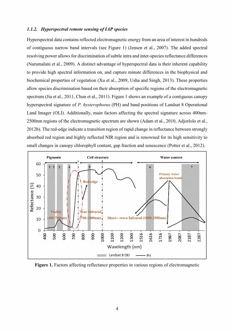
1.1.2. Hyperspectral remote sensing of IAP species
Hyperspectral data contains reflected electromagnetic energy from an area of interest in hundreds
of contiguous narrow band intervals (see Figure 1) (Jensen et al., 2007). The added spectral
resolving power allows for discrimination of subtle intra and inter-species reflectance differences
(Narumalani et al., 2009). A distinct advantage of hyperspectral data is their inherent capability
to provide high spectral information on, and capture minute differences in the biophysical and
biochemical properties of vegetation (Xu et al., 2009, Usha and Singh, 2013). These properties
allow species discrimination based on their absorption of specific regions of the electromagnetic
spectrum (Jia et al., 2011, Chun et al., 2011). Figure 1 shows an example of a contiguous canopy
hyperspectral signature of P. hysterophorus (PH) and band positions of Landsat 8 Operational
Land Imager (OLI). Additionally, main factors affecting the spectral signature across 400nm-
2500nm regions of the electromagnetic spectrum are shown (Adam et al., 2010, Adjorlolo et al.,
2012b). The red-edge indicate a transition region of rapid change in reflectance between strongly
absorbed red region and highly reflected NIR region and is renowned for its high sensitivity to
small changes in canopy chlorophyll content, gap fraction and senescence (Potter et al., 2012).
Figure 1. Factors affecting reflectance properties in various regions of electromagnetic
5
spectrum and a comparison of contiguous spectral signature of P. hysterophorus (PH) and
discrete band positions of multispectral data (Landsat 8 OLI).
Whereas airborne and spaceborne hyperspectral image data have been known to generate highly
reliable IAP species classifications (Yang and Everitt, 2010, Yang et al., 2011, Olsson and
Morisette, 2014), they are often costly and have limited global coverage, and therefore currently
limited to a small number of projects (Narumalani et al., 2009, Huang et al., 2009, He et al.,
2011). Furthermore, existing sensors e.g. EO-1 Hyperion and Compact High Resolution Imaging
Spectrometer (CHRIS) are insufficient (Buckingham and Staenz, 2008); hence there are
significant data gaps in most invaded areas. Alternatively, leaf and canopy level hyperspectral
measurements using field spectrometers have been used to understand the reflectance properties
of various species for discrimination purposes (Schmidt and Skidmore, 2003, Adam and
Mutanga, 2009, Fernandes et al., 2013), to estimate biochemical properties such as nitrogen
content (Bajwa et al., 2010, Wei et al., 2012), chlorophyll content (Xu et al., 2009) and leaf-
water content (De Jong et al., 2014, Mirzaie et al., 2014). Canopy hyperspectral data are cheaper
to acquire and allow for in-depth understanding of spectral signatures of IAP species in a
heterogeneous landscape for mapping. For example, Fernandes et al. (2013) note that optimal
spectral bands selected from canopy hyperspectral measurements are essential for selecting most
suitable satellite imagery for mapping. However, the adoption of canopy hyperspectral data is
often limited by their characteristic high data dimensionality, often resulting into lower
classification accuracies and high computational requirements (Pal and Foody, 2010). A novel
approach to select optimal spectral subset of bands that yield improved classification accuracy
and optimises computation is therefore proposed in chapter 2 of this dissertation.
1.1.3. Multispectral remote sensing of IAP species
For decades, multispectral remotely sensed data has been adopted to monitor the spread and
determine the distributions of IAP’s. Multispectral sensors capture reflected and emitted energy
from an area of interest in multiple broad band intervals (i.e. ~4 to 36) of the electromagnetic
spectrum (see Figure 1) (Jensen et al., 2007). To date, a wealth of historical and current low or
no cost multispectral data at different spatial and temporal resolutions exist (see Table 1). As a
result, researchers have extensively applied remotely sensed data from multispectral sensors such
as MODIS, NOAA/AVHRR, Landsat, ASTER and SPOT to monitor the spread and determine
the spatial distributions of IAP’S (Huang and Asner, 2009, Viana and Aranha, 2010, Zong et al.,
2010, Frazier and Wang, 2011, Qu et al., 2011). For example, moderate spatial resolution (30m)
data from Landsat TM, with six spectral bands in visible (VIS), near-infrared (NIR) and

6
shortwave infrared (SWIR) and SPOT 5, with 4 spectral bands in VIS, NIR and SWIR and a
10m spatial resolution have allowed for the detection of Spartina alterniflora (saltmarsh
cordgrass) with overall accuracies of 71% to 78.8% in China (Zong et al., 2010). Laba et al.
(2008) obtained overall accuracies of between 64.9% and 73.6% when mapping Trapa natans
(water chestnut), Phragmites australis (common reed), and Lythrum salicaria (purple
loosestrife) using Quickbird data (4 spectral bands in the VIS and NIR at 2.4m spatial
resolution). Generally, medium resolution sensors have been found useful for mapping larger
patches, i.e. >0.5 ha (Arzandeh and Wang, 2003).
Recent studies (Lantz and Wang, 2013, Adelabu et al., 2013, Müllerová et al., 2013) have shown
that very high spatial resolution data (i.e. <1m) combined with additional narrow bands, i.e. red
edge and yellow have high capability of detecting and discriminating species. Using Worldview-
2 imagery, with 8 multispectral bands and 2m spatial resolution for instance, Lantz and Wang
(2013) mapped the distribution of Phragmites australis (common reed) in a coastal wetland,
achieving a classification accuracy of 94%. Generally, developments in multispectral
instruments are expected to enable higher classification accuracies and provide further
opportunities for testing classification algorithms used for discriminating and determining IAP’s
distributions. Such new generation sensors include Worldview-3, which offers very high spatial
resolutions (1.24m-multispectral, 31cm-panchromatic, 3.7m-SWIR 3.7m, and 30m-Clouds,
Aerosols, Vapours, Ice, and Snow bands (CAVIS)) with super spectral resolution (8 VNIR
bands; 8 SWIR bands and 12 CAVIS bands). However, whereas very high resolution data may
provide higher classification accuracy, they are often costly for operational applications.
Consequently, data accessibility and cost from heritage missions such as SPOT and Landsat
provide an opportunity for mapping the distribution and patch sizes of P. hysterophorus in
infested areas of Kwa Zulu Natal province. SPOT 6 (launched in 2012), in comparison to its
predecessor, has an improved spatial resolution (i.e. 6m - multispectral bands, 1.5m -
panchromatic band) and four spectral bands in Visible and NIR regions. On the other hand,
Landsat 8 (launched in 2013) has 10 spectral bands in Visible, NIR, SWIR and TIR regions of
the electromagnetic spectrum. These datasets were evaluated for mapping the distribution and
patches of P. hysterophorus in Chapter 3 of this study. Table 1 outlines some of the potential
data for mapping IAP species.

7
Table 1. Potential multispectral data for mapping IAP species.
Moderate Resolution Sensors (<30m)
Sensor PAN Multispectral Swath
width
Revisiting
Period
Archive Programmable Accessibility
Landsat 8
OLI
15m 30m (VNIR,
CB, 2×SWIR
185km 16 days 2013 No Free
ASTER 15m (V +
2×NIR), 30m
(5×SWIR)
1999 Yes US$80/60km2
High Resolution Sensors (<10m)
SPOT 5 2.5m 10m (VNIR)
& 20m
(SWIR)
60km/120km 26 days 2002 Yes Free for non-
commercial
use in SA
SPOT 6 & 7 1.5m 6m (VNIR) 60km 1 to 3
days
2013 Yes Free for non-
commercial
use in SA,
otherwise
US$5.15/km2
Quickbird 0.6m 2.4
(VNIR+RE)
16.5km 1 to 3
days
2002 Yes US$16/km2
RapidEye 6.5m
(VNIR+RE)
1 day 2008 Yes US$1.28/km2
IKONOS 0.82m 3.2m (VNIR) 11km 1 to 3 1999 Yes US$10/km2
Very High Resolution Sensors (<0.5m)
GeoEye-1 0.5m 2m (VNIR) 15.2km 1 to 3 2008 Yes US$16/km2
Pleiades 0.5m 2m 20km Daily 2012 Yes US$13/km2
WorldView-
2
0.5m 2m (V, CB,
2×NIR, RE, Y)
16.4km Daily 2009 Yes US$16/km2
WorldView-
3
0.31m
nadir/
0.34
off-
nadir
1.24m
nadir/1.38m
off-nadir (V,
CB, 2×NIR,
RE, Y); 3.70m
nadir/4.10m
off-nadir
(8×SWIR) &
30m nadir
(CAVIS)
13.1 km <1 day 2014 Yes US$32/km2
Acronyms : ‘V’=standard Blue, Green & Red bands; ‘CB’ =coastal/aerosol ‘NIR’=Near Infrared band; ‘Y’=Yellow
band, ‘RE’=Red Edge, ‘SWIR’=Short-wave Infrared, ‘TIR’=Thermal Infrared band, ‘CAVIS’=Clouds, Aerosol,
Vapours, Ice and Snow bands
1.1.4. Classification algorithms and vegetation indices for discriminating IAP species
For decades, various parametric algorithms such as ISODATA, Parallelpiped, Minimum
Distance to Means (MDM) and Maximum Likelihood Classifier (MLC) have been used on
remotely sensed data. Such algorithms have a priori assumptions that the data is normally
distributed and utilise image statistics (such as mean, standard deviation and covariance
matrices) to allocate pixels to clusters (Memarian et al., 2013). Arzandeh and Wang (2003)
achieved overall accuracies of between 82% and 87% using MLC and multispectral data from
SPOT, Landsat and Indian Remote Sensing Satellite (IRS) for monitoring Phragmites australis
8
(Common reed). Whereas ISODATA and MLC have been the most commonly used parametric
algorithms, for monitoring and determining IAP’s spatial distribution (Theriault et al., 2006,
Viana and Aranha, 2010, Everitt et al., 2005), other studies (Chi et al., 2008, Mountrakis et al.,
2011) have established that classification using parametric algorithms is tedious (requiring
enormous training samples), and yield poor classification results when highly dimensional data
and small training sample are used. Furthermore, parametric algorithms do not take into account
the complexity of class distributions in multi-temporal datasets, i.e. non-normality and
multimodality (Gavier-Pizarro et al., 2012).
On the other hand, non-parametric machine learning algorithms such as Artificial Neural
Networks (ANN), Spectral Angle Mapper (SAM), Random Forests (RF), Decision Trees (DTs)
and Support Vector Machines (SVMs) have no prior assumptions about the data, can incorporate
ancillary data, and are flexible and adaptable (Carpenter et al., 1997). Such algorithms have
recently been successfully adopted on both hyperspectral and multispectral data (Pal and Mather,
2004, Gavier-Pizarro et al., 2012, Adelabu et al., 2013, Yagoub et al., 2014, Atkinson et al.,
2014). SVM was adopted in Chapter 2 and 3 of this dissertation for spectral discrimination and
mapping the distribution and patches of, P. hysterophorus.
1.1.5. Challenges and opportunities for discrimination of P. hysterophorus
In hyperspectral remote sensing of vegetation, challenges such as multicollinearity and
multidimensionality are commonly encountered (Adjorlolo et al., 2013, Peerbhay et al., 2013,
Pal, 2006). The Hughes phenomenon, also known as the ‘curse of dimensionality’ reduces the
performance of the classifier when there is limited training data (Hughes, 1968). In addition,
narrow and contiguous spectral bands in hyperspectral data are often correlated with one another,
resulting in highly unstable parameter estimates hence, increasing the generalization error of a
classifier (Clevers et al., 2007, Mirzaie et al., 2014). Although several techniques have been
proposed to overcome these challenges, none of them has been proven superior (Adam and
Mutanga, 2009, Jia et al., 2011). This provides an opportunity to test the performance of other
innovative techniques for dimensionality reduction and to improve classification accuracy.
In multispectral image classification, phenomena such as mixed pixels and spectral confusion
are common, where the former refers to pixels that contain two or more classes and the latter
occurs when two or more classes have similar reflectance properties (Hsieh et al., 2001, Yang et
al., 2011). Medium resolution (i.e. 10 – 30m) images often have pixels that cover larger areas,
hence patches of P. hysterophorus that cover smaller proportion of each pixel are likely to be

9
missed by the hard classifiers. For example, using Landsat TM to distinguish between native
vegetation and an invasive species Pennisetum ciliare (buffelgrass), Olsson et al. (2011) found
very low classification accuracy due to the heterogeneity of the landscape which resulted in
mixed pixels.
Generally, studies have indicated that higher spatial resolution image data (i.e. <10m) offer
greater resolving power, hence a higher probability that smaller patches can be detected with
higher accuracy (Jensen, 1983, Dorigo et al., 2012). However, this is not always the case as
spectral variability within one species, i.e. intra-species variability may be increased, resulting
in spectral confusions and reduced classification accuracy. As noted by Hsieh et al. (2001), high
spatial resolution imagery provides a wealth of spatial information about various objects on the
ground; however the classification results are not always as promising as can be expected. In
addition, it is challenging to distinguish IAP species from native species using discrete and broad
wavelengths in multispectral images, since these are less capable of defining minute spectral
differences between species. P. hysterophorus has sporadic growth and rapid spread; hence
usually have varying patch sizes. This variability in patch sizes and different phenology of one
species in an image may yield high uncertainty in the derived classification (Muad and Foody,
2012). As a result, a fair compromise between the spectral and spatial resolutions is fundamental
when choosing data for mapping IAP’s.
1.2. Research problem
Parthenium hysterophorus (Parthenium weed) has been identified as one of top 7 most
devastating weeds in the world. Considerable impacts on ecosystem processes and functions,
biodiversity, agriculture and human health have been reported. Hence, eradication and control
of the species has recently become the focus in literature, with several interventions being
proposed. In South Africa, P. hysterophorus invades savanna landscapes of northern KwaZulu-
Natal where it has become dominant. As a result, it need to be eradicated and controlled to
prevent further spread and introductions into new areas. Accurate and up-to-date information on
the locations and distribution of P. hysterophorus is required for designing relevant mitigation
measures. However, traditional field-based methods are costly, tedious, unsustainable and
inappropriate for large and inaccessible areas. In that regard, remotely sensed data from
hyperspectral and multispectral sensors can be exploited for providing useful information critical
for effective weed management and site prioritisation.
This study sought to address the following research problems:
10
i. The inherent high dimensionality in hyperspectral data reduces classification accuracy
due to Hughes effect.
ii. Among existing feature selection techniques, there is no single technique that has been
proved superior in literature, hence an opportunity exist to explore other techniques.
iii. The usefulness of the spatial and spectral configurations of OLI and SPOT 6 datasets
for characterizing the patches of P. hysterophorus, have never, to the best of our
knowledge, been explored.
1.3. Aim and Objectives
1.3.1. Aim
The aim of this study was to explore the capability of hyperspectral and multispectral data for
discriminating and mapping Parthenium hysterophorus.
1.3.2. Objectives
The objectives of the study were:
(i) To determine optimal subset of spectral bands from canopy hyperspectral data for accurately
discriminating P. hysterophorus and co-existing species.
(ii) To evaluate capability of multispectral data from Landsat 8 OLI and SPOT 6 for determining
P. hysterophorus distribution and patch sizes.
1.4. Research questions
This study attempted to address to the following research questions:
i. What is the optimal subset of bands for discriminating P. hysterophorus from its co-
existing species?
ii. How can classification accuracy be improved by reduced subset of bands versus entire
dataset?
iii. What is the utility of the spectral and spatial configurations of multispectral data (i.e.
OLI and SPOT 6) in mapping the patches of P. hysterophorus?

11
1.5. Scope of the study
This study explored the capability of hyperspectral and multispectral data for discriminating and
mapping P. hysterophorus in the Savanna landscapes of northern Kwa Zulu-Natal province. A
robust classification algorithm, i.e. Support Vector Machines (SVM) was used with canopy
hyperspectral and multispectral datasets to discriminate P. hysterophorus from co-existing
species and to determine its distribution and patch sizes, respectively. Specifically, Chapter 2
presents the potential of an innovative hierarchical approach to deal with high dimensionality in
hyperspectral data and to improve classification accuracy of P. hysterophorus while Chapter 3
presents the capability of multispectral data for providing accurate information on P.
hysterophorus distribution and patch sizes. According to (Turner et al., 2003), this information
is fundamental in understanding the ecological links to the diversity, structure and processes of
the ecosystem and habitats changes.
1.6. Study area
The study area is located in the northern part of Kwa Zulu-Natal province, South Africa
(Latitudes 26°45′ to 27°7′ and Longitudes 22°7′ to 32°20′; Figure 2). The area lies in the summer
rainfall belt, with an annual range of 500 – 2000mm. Temperatures are cooler (13.9 oC) during
winter and warm (21.7oC) in summer (Atkinson et al., 2014). The area falls within the savanna
biome, characterised by open Lowveld savanna vegetation, shrubs and grasses. Common tree
species include; Umbrella thorn (Acacia tortillis), Sweet thorn (Acacia karroo), and Tamboti
(Spirostachys Africana) while grass species include Spreading prinklegrass (Aristida congesta
subsp. Barbicollis) and Pinhole grass (Bothriochloa insculpta) that occur in highly disturbed
areas and Redgrass (Themeda triandra) and Spear grass (Heteropogon contortus) that dominate
less disturbed areas. The prevalence of non-native plants has become a serious problem in the
area where IAP’s such as P. hysterophorus have become increasingly prolific. P. hysterophorus
infestations are particularly evident along roads, in croplands, along fences and backyards,
disturbed grasslands and protected areas. P. hysterophorus was first recorded in Kwa Zulu Natal
province in 1880 and again after the floods in 1984 caused by Cyclone Demoina (McConnachie
et al., 2011). As a result, field surveys showed that Ndumo Game Reserve is one of the most
heavily infested reserves in the province; hence communal rangelands surrounding the reserve
are also infested. Spectroscopy data (Chapter 2) was collected within Ndumo Game Reserve (26°
54' 43'' S and 32° 15' 48'' E, total area 102 km2), while Landsat 8 OLI and SPOT 6 images
(Chapter 3) covered the reserve, communal farmlands and settlements (26o45′00″S and 32o
00′00″E).

12
Figure 2. Study area
1.7. Chapter outline
CHAPTER 1: GENERAL INTRODUCTION
The chapter provides a general background to Parthenium hysterophorus, including its
description, distribution and impacts, the advantages of using remote sensing data and algorithms
for discriminating IAP species. An overview of common challenges in remote sensing of IAP’s
are also briefly discussed. Additionally, research objectives, description of the study area, and
the scope of the study are outlined.
CHAPTER 2: DETERMINING THE OPTIMAL SPECTRAL SUBSET FOR
DISCRIMINATING PARTHENIUM HYSTEROPHORUS
This chapter adopts field spectroscopy data for discriminating P. hysterophorus and co-existing
species. A novel approach integrating statistical filters and Support Vector Machines – Recursive
Feature Elimination (SVM-RFE) for dealing with multidimensionality and co-linearity is
proposed. The performance (i.e. classification accuracy) of hierarchically selected bands was

13
compared to the performance of entire spectral data and a combination of 20 best spectral bands
selected by SVM-RFE.
CHAPTER 3: EVALUATING THE CAPABILITY OF LANDSAT 8 OLI AND SPOT 6 FOR
DISCRIMINATING INVASIVE ALIEN SPECIES WITHIN THE SAVANNA LANDSCAPES
OF KWAZULU-NATAL, SOUTH AFRICA.
This chapter explores the utility of multispectral data from Landsat 8 OLI and SPOT 6 sensors
for discriminating P. hysterophorus. The goal was to determine the optimal data for providing
useful information on the distribution and patch sizes of P. hysterophorus for control and
eradication, environmental and resource management and conservation planning. A robust
algorithm, Support Vector Machines was used for classifying both datasets. Each dataset was
evaluated using confusion matrix.
CHAPTER 4: SYNTHESIS AND CONCLUSION
This chapter presents a synthesis of the main findings of study, discuss the relevance of the
results, make necessary recommendations for future studies and provides the limitations of the
study.

14
CHAPTER 2
DETERMINING THE OPTIMAL SPECTRAL SUBSET FOR
DISCRIMINATING PARTHENIUM HYSTEROPHORUS
2.1. Introduction
Hyperspectral remotely sensed data have been proven to be valuable for discriminating woody
vegetation, herbaceous plants and grass species in sub-tropical and savanna grasslands
(Adjorlolo et al., 2013, Mansour et al., 2012, Adam and Mutanga, 2009, Jia et al., 2011, Peerbhay
et al., 2013, Atkinson et al., 2014). The major advantage of hyperspectral data is their narrow
spectral bandwidths and large number of contiguous spectral bands, which are useful for
distinguishing subtle differences in vegetation features (He et al., 2011). The higher sensitivity
of hyperspectral instruments to biophysical and biochemical reflectance properties of various
vegetation types make such instruments useful for characterizing plants species (Bajwa et al.,
2010, Jensen, 1983, Daughtry et al., 2000, Xu et al., 2009). However, for species discrimination,
the utility of hyperspectral data has been commonly impeded by its inherent properties such as
multidimensionality and multi-collinearity (Demir and Ertürk, 2008). Hughes (1968) observed
that the addition of more dimensions lead to a decrease in classification accuracy when training
sample is small, i.e. n < p. This phenomenon, also referred to as “the curse of dimensionality”
or Hughes effect, causes highly unstable parameter estimates and hence high generalization
errors for the classifier (Clevers et al., 2007). For example, Tadjudin and Landgrebe (1998)
determined that parametric classifiers such as Maximum Likelihood (ML) are less capable of
estimating mean and covariance statistics from multidimensional data, hence yield undesirable
classification accuracies, particularly with limited training data.
More robust non-parametric classifiers such as Support Vector Machines (SVM) have been
reported to efficiently handle noise and multidimensionality in hyperspectral data (Pal and
Mather, 2004, Cortes and Vapnik, 1995). Studies (Pal and Mather, 2004, Pal, 2006) have
adopted SVM classification algorithm using large training samples (>100 pixels per class) to
overcome the Hughes effect. The major challenge is that acquisition of large training samples
can be tedious, costly and time consuming, particularly where areas to be sampled are
inaccessible (Adam and Mutanga, 2009, Jia et al., 2011). Using Airborne Visible InfraRed
Imaging Spectrometer (AVIRIS) and Digital Airborne Imaging Spectrometer (DAIS) datasets,
Pal and Foody (2010) observed a significant decrease in SVM classification accuracy with an
increase in dimensionality for small training data (≤ 25 pixels per class). The authors concluded
15
that the Hughes effect was more prevalent when a small training data was used. In this regard,
feature selection and dimensionality reduction is fundamental to aid the classifier to use only the
relevant subset of predictor features that capture relevant properties of the response variable
(Camps-Valls and Bruzzone, 2005, Pal and Foody, 2010). Additionally, feature selection may
reduce the computational costs related to processing hyperspectral data, thus reducing training
time and simplifying classification tasks (Pal, 2009). Feature selection and dimensionality
reduction prior to classification have consequently become necessary in hyperspectral data
analysis and has led to better classification accuracies and increased computational efficiency
(Zhang and Ma, 2009, Pal and Foody, 2010, Löw et al., 2013).
Feature extraction techniques such as principal component analysis (Mather, 2004), maximum
noise fraction (Green et al., 1988) and partial least squares regression (Wold, 1995) transform
the original feature-space in order to provide fewer de-correlated components sorted by their
signal to noise ratio (SNR) (Huang et al., 2004). However, these techniques do not automatically
select relevant spectral bands for the classification model (Chun and Keleş, 2010). Critically,
these techniques use all spectral bands in the transformation, including redundant bands and may
be insensitive to subtle differences that are helpful for the discrimination of species (Tsai et al.,
2005, Yao and Tian, 2003). Filter-based techniques on the other hand evaluate the intrinsic worth
of each feature based on some relevance index such as correlation coefficients, test statistics or
information theory (Pal, 2009, Guyon and Elisseeff, 2006). Whereas they are computationally
efficient, they do not use a classifier to evaluate the performance of each feature and often ignore
the impact of class labels (Deng et al., 2013). Conversely, wrapper techniques such as Support
Vector Machines - Recursive Feature Elimination (RFE) (Guyon et al., 2002) use a classifier as
a ‘black-box’ to evaluate the predictive worth of each feature while embedded techniques
simultaneously perform feature selection and classification (Guyon and Elisseeff, 2006).
However, the technique's high computational requirements has limited its wide adoption with
commonly used classifiers (Pal, 2009).
Nevertheless, SVM-RFE (Guyon et al., 2002) are often preferred over filter-based and embedded
models due to their high performance and ability to overcome orthogonality assumptions. This
is achieved by adopting mutual information between features and using support vectors
exclusively as a decision function (Pal and Foody, 2010). Typically, the technique uses the
weight value calculated during the training stage of SVM as the ranking criterion for evaluating
features (Zhang and Ma, 2009, Pal and Foody, 2010). Pal (2009) compared the performance of
Greedy Feature Flip algorithm, Iterative Search Margin-based algorithm and SVM-RFE and
16
found that the performance of all the approaches were comparable when using best combination
of 20 features selected by respective algorithms from both DAIS and AVIRIS datasets. Pal and
Foody (2010) showed that smaller subsets of selected spectral bands ranked by SVM-RFE,
Random Forest and mutual information-based max-dependency (mRMR) techniques were
equally significant to achieve comparable accuracies with the entire dataset. Other studies
(Zhang and Ma, 2009, Li et al., 2011) found that SVM-RFE was affected by the dataset’s noise
and has high computational requirements. Generally, a number of studies, among others (Adam
and Mutanga, 2009, Pal and Foody, 2010, Jia et al., 2011) have shown that different approaches
result in dissimilar sets of optimal features due to different number and separability of classes,
study objectives and nature of the dataset. This indicates that there is no single superior
technique that can be used to select an optimal subset of spectral bands for improving
classification accuracy (Yang et al., 2005). Therefore, this study presents the potential of a
hierarchical approach for dimensionality reduction and subset size selection for improved
classification accuracy.
The study implements an integration of both filter and wrapper approaches to effectively reduce
dimensionality and concurrent selection of optimal subset of spectral bands for discrimination
of IAP species in the study area. The first step of analysis involves Kruskal-Wallis analysis of
variance (ANOVA) to identify spectral bands with significant differences in median at p < 0.05.
In the second step, inter-band correlation and Area under Receiver Operating Characteristic
curve (AUC-ROC) analysis are performed to remove redundancy while retaining relevant
spectral bands using AUC as a goodness measure. In the final step, we apply SVM-RFE to select
a minimum subset of spectral bands which together yield improved classification accuracy.
Using spectral reflectance characteristics on an area characterized by P. hysterophorus IAP and
co-existing species, we compare classification accuracy from the hierarchical approach against
the accuracy achieved from entire spectral dataset (n = 1633) and a combination of 20 best
spectral bands ranked by SVM-RFE. The choice of IAP species discrimination, particularly P.
hysterophorus in this study was based on several challenges in management of the species and
mapping of its distribution using conventional methods.
2.2. Materials and methods
2.2.1. Species description
Parthenium hysterophorus (Parthenium weed) is regarded as one of the seven most aggressive
and problematic weeds in the world (Dhileepan 2007). It is known to invade agricultural fields,

17
hence reduce agricultural production and affect livelihoods (Dhileepan, 2007, Patel, 2011). The
weed is also known to invade ecological systems, reducing biodiversity and compromising
ecological integrity and the ability to provide ecosystem goods and services (Dhileepan, 2007,
Patel, 2011). Typically, P. hysterophorus rapidly invades and colonizes disturbed areas such as
abandoned croplands, building peripheries, roadsides, fallow and overgrazed lands, waste lands
and cultivated fields (McConnachie et al., 2011). Each plant grows sporadically and rapidly,
flowers and produces approximately 25 000 light seeds, which are dispersible for longer
distances by vehicles, water, animals, farm machinery and wind (Javaid et al., 2009,
McConnachie et al., 2011, Dogra et al., 2011).
Throughout its lifecycle, P. hysterophorus releases toxic chemicals which inhibit germination
and growth of co-existing species (McConnachie et al., 2011). This leads to a decline in pasture
production (Dhileepan, 2007), dry grass biomass (Nigatu et al., 2010) and natural habitats and
biodiversity (Patel, 2011). Prolonged exposure and excessive consumption has been reported to
result in health complications in human populations, declined quality of milk and meat products
from cattle and degenerative changes in liver and kidney of sheep and buffalo (Patel, 2011).
Therefore, to mitigate these impacts, early detection is necessary for design and implementation
of management and eradication measures. Hence a need to determine the most optimal bands for
spectral discrimination of P. hysterophorus, valuable for mapping using remotely sensed
imagery.
2.2.2. Data collection
2.2.2.1. Field sampling
Field survey of several P. hysterophorus infested sites was conducted to identify the distribution
of P. hysterophorus. During the survey, it was also ensured that the conditions in which P.
hysterophorus exists, including co-existing species were identified prior to spectral data
collection. Based on the survey, 1×1m plots of homogeneous (>90%) juvenile P. hysterophorus
canopy cover and co-existing species were delineated. A total of 149 plots with P. hysterophorus
and co-existing species were then randomly selected from the study area (see Table 2). This was
done to account for intra-species variability and to ensure that both P. hysterophorus and co-
existing species were well represented. In each 1×1m plot, a minimum of three random positions
were selected for hyperspectral measurements.
2.2.2.2. Hyperspectral data collection

18
Spectral reflectance characteristics were acquired using a Spectral Evolution PSR-3500
Spectrometer (Spectral Evolution, Inc. © 2014) with a 350nm–2500nm spectral range. The
spectrometer has ~3.5nm spectral resolution at 350-1000nm, 10nm at 1500nm and 7nm at 2100.
The spectral bands from 350-1000nm, at 1500nm and at 2100nm have nominal spectral sampling
intervals of 1.5nm, 3.8nm and 2.5nm, respectively. The spectral measurement unit consisted of
spectrometer, a handheld Personal Digital Assistant (PDA) device and a fiber optic cable
attached to the pistol grip for easy handling. Garmin Montana 650 standard GPS with ±3m
accuracy was used for locating and navigating to the sampled plots.
P. hysterophorus and co-existing species canopy reflectance measurements were taken from
1×1m plots in early December 2014 (see Table 2 and Appendix 1). The scale of measurement
ensured that the spectral measurements were a representative mixture of radiance as determined
by the proportion, physical arrangement and reflective and transitive properties of plants
components (Clark and Roush, 1984). Each spectral curve was visualized on a PDA and noisy
measurements (including those affected by shadows) replaced by new measurements before
being recorded. Each observation measured by the spectrometer was an average of 10 scans, at
optimized integration time with a dark current correction and plots were tagged with a GPS
coordinate and a photograph. Each plot was represented by an average of 3-5 pure spectral
measurements, taken from distinct random positions within a plot. A fiber optic cable with a 25o
FOV was consistently held at nadir angle. Also, an observation distance of 0.5m above each
homogeneous canopy was maintained in all measurements. This yielded a circular surface area
measurement (i.e. instantaneous field of view - IFOV) with a radius of approximately 11.08cm.
In each case, the IFOV was significant to measure the radiances from targets without the
interference of background reflectance. To normalize target measurements and to minimize the
influence of the change of atmospheric conditions and solar irradiance (Mirzaie et al., 2014,
Darvishzadeh et al., 2008), a white reference panel (spectralon) reflectance was taken before and
after each plot measurements. All reflectance measurements were taken on cloudless or near
cloudless conditions between 10:00 and 14:00 South African Standard Time (GMT+02:00). This
was necessary to limit the variability due to changes in sun angle (Bajwa et al., 2010); to avoid
excessive shadows (Menges et al., 1985) and to minimize atmospheric perturbations and
Bidirectional Reflectance Distribution Function (BRDF) effects (Darvishzadeh et al., 2008).

19
Table 2. The number of plots and measurements per species
Species Number of Plots Number of
measurements
P. hysterophorus (PH) 65 195
Acacia trees (AT) 33 99
Grass species (GS) 19 57
Other plant species (OPS) 32 96
2.2.3. Pre-processing and analysis
2.2.3.1. Pre-processing
The original spectral measurements consisted of 1024 spectral data points, with varying spectral
resolution and sampling interval. These were interpolated to 1nm using Cubic spline
interpolation, yielding 2151 spectral data points. The interpolation to finer sampling intervals
was necessary to minimize errors that may arise from varying spectral sampling interval and
detector steps of the spectrometer (Clark and Roush, 1984, Gardner, 2003). The noisy spectral
bands (350-399nm; 1350-1465, 1790nm-1960nm and 2350nm-2500nm) were removed from
further analysis (Thenkabail et al., 2004). Noise removed spectral data were then subjected to
Savitzky Golay Filtering (Savitzky and Golay, 1964) experimental procedures with linear and
quadratic polynomials (i.e. p = 1, 2, 3) and different window sizes (i.e. m = 5, 11, 25). Savitzky
Golay Filter with parameters p = 2 and m = 11, resulted in relatively smooth spectral curves,
while closely maintaining the absorption features across all wavelengths (see Figure 3). Noise
removal and Savitzky Golay (SG) filtering resulted in 1633 spectral data points for further
analysis. Cubic spline interpolation and SG filtering were performed using “prospectr” package
(Stevens and Ramirez–Lopez, 2014) in R Statistical software.
2.2.3.2. Data analysis
Due to the aforementioned challenge in determining the optimal spectral bands from high
dimensional spectral data and lack of a single superior technique for selecting optimal spectral
bands, we implemented an innovative hierarchical technique consisting of Kruskal-Wallis
ANOVA, inter-band τ correlation and AUC-ROC variable importance and SVM-RFE. Kruskal-
Wallis ANOVA (Kruskal and Wallis, 1952) and post hoc Dunn’s test (Dunn, 1964) were used
to test the null hypothesis that there is no significant differences between the median spectral
signatures of P. hysterophorus and its co-existing species at 95% significance level (p < 0.05).
20
Kruskal-Wallis ANOVA is a rank-based non-parametric test used to compare multiple
independent samples. Contrary to one-way ANOVA, it calculates a unique initial table with p-
value of the test for all the wavelengths and all co-existing species simultaneously (Quinn and
Keough, 2002). The difference between medians of spectral signatures was tested as opposed to
difference of means since Kruskal-Wallis ANOVA does not assume a normal distribution of the
data (Lehman, 1975). Additionally, Kruskal-Wallis ANOVA is robust on different sample sizes
(Quinn and Keough, 2002).
Since the dimensionality of the data remained high even after significantly different spectral
bands were identified by Kruskal-Wallis ANOVA, we implemented inter-band correlation
analysis using Kendall’s tau (τ) and AUC-ROC variable importance. The correlation analysis
was implemented to identify and remove redundant spectral bands with a correlation coefficient
of >0.9, while AUC-ROC variable importance was used to estimate the importance of each
retained band (by correlation analysis) for discriminating P. hysterophorus and co-existing
species. Kendall’s τ (Joe, 1990) is a distribution-free measure of concordance between two
observed variables. A pair of points (xi, yi) and (xj, yj ) are said to be concordant if (yj − yi)/(xj −
xi) > 0 and discordant if (yj − yi)/(xj − xi) < 0 (Joe, 1990). In the current study, a correlation
coefficient of >0.9 was considered highly correlated for spectral bands of P. hysterophorus and
co-existing species being redundant. The spectral bands with correlation coefficient less than the
threshold of 0.9 were subjected to AUC-ROC variable importance available in “caret” package
(Kuhn, 2008) to determine their individual inter-species discriminatory ability. AUC-ROC
variable importance for multiple classes uses one-against-all strategy to perform ROC curve
analysis on each band with a series of cutoffs being applied to predict classes. For each cutoff, a
two dimensional space is formulated, where sensitivity is the vertical axis and 1-specificity is the
horizontal axis (see Formulae 1 and 2). Area under the ROC curve (AUC) is then calculated for
each class using trapezoid rule and the maximum AUC across the relevant pair-wise AUC's is
used as the variable importance measure. In essence, AUC is used as a goodness measure for
judging whether each band is important or not, where an area of 1 represents absolute importance
and an area of 0.5 indicates that the spectral band has no discriminative power (Deng et al.,
2013). Inter-band τ correlation and AUC-ROC variable importance allow filtering of redundant
and less important spectral bands, while maintaining those with high discriminating power
before SVM-RFE is applied.
Sensitivity = TP/(TP + FN) [1]
Specificity = TN/(TN + FP) [2]

21
Where; TP, FN, TN, FP denote true positive, false negative, true negative and false positive
respectively.
As a final step, we applied a wrapper feature selection approach, viz. Support Vector Machines
- Recursive Feature Elimination, to automatically choose the optimal subset of features that yield
high classification accuracy. SVM-RFE is a robust wrapper feature selection technique that uses
an objective decision function (1/2)||w||2 of SVMs to select optimal nested subset of features
ordered by their discriminatory ability (Guyon et al., 2002). It uses backward feature elimination
strategy, where a full set of features are used as the starting point of feature selection and features
that cause changes in the decision function are progressively eliminated. At each iteration, the
ranking scores of features are computed from coefficients of the weight vector w and the features
with least score wi2 are recursively eliminated (where wi
2 represents the corresponding ith
component of w). Unlike other feature selection techniques, SVM-RFE uses mutual information
between features and the decision function is based solely on support vectors, thus eliminating
orthogonality assumptions (Guyon et al., 2002, Pal and Foody, 2010). A detailed discussion of
SVM-RFE can be found in Guyon et al. (2002) and Pal (2006).
2.2.4. SVM classification and validation
The SVM classification algorithm was applied to verify that selected wavelengths by the
previous analysis can reliably discriminate P. hysterophorus (PH) and co-existing species. This
was done to determine the optimal hyperplane with maximum margin (Boser et al., 1992). The
procedure ensures that the samples with class labels ±1 are located on the either side of the
hyperplane and the distance (or optimal margin) of the closest training vectors (support vectors)
is maximized, thus reducing the generalization error of the overall classifier (Vapnik, 1999). A
training sample N can be represented by (yi, xi), i = 1, 2,..N), where yi represents class labels ±1
and xi is a feature vector with n components. The linear SVM classifier is represented by the
function f(x, α) → y, where α is the parameter of the classifier (Mercier and Lennon, 2003). In
a nonlinearly separable problem, a regularization parameter C and kernel parameter σ are
introduced. C is used to control the trade-off between the maximization of the margin between
the training data vectors, decision boundaries and margin errors of the training data. On the other
hand, σ is used to control the width of the kernel (i.e. polynomial, radial basis function (RBF) or
sigmoid kernel), allowing SVM to distinguish multi-modal classes in a high dimensional space
(Foody and Mathur, 2004). Decomposition approaches such as one-against-one and one-against-
all have been developed to deal with multiple-class classification problems, since the original
SVMs were developed for two-class problems. One-against-one approach applies (M(M −

22
1))/2 classifiers on each pair of classes and the mostly computed class label is kept for each
vector, while one-against-all approach iteratively applies M classifiers on each class against the
rest. M is the number of classes (Hsu and Lin, 2002, Mercier and Lennon, 2003). We used one-
against-all approach with an RBF kernel and a 10-fold cross validation (CV) within “kernlab” R
package (Karatzoglou et al., 2005). The tuning parameters for the classification model were
selected by evaluating candidate pairs of a constant σ directly estimated from the training data
by “sigest” function within “kernlab” and “caret” packages (Kuhn, 2008), and nine values of
possible C parameters, i.e. 0.25, 0.5, 1, 2, 4, 8, 16 and 32. Additional classification experiments
were performed on entire spectral dataset and a combination of 20 best spectral bands ranked by
SVM-RFE for comparison with the hierarchical approach. Classification accuracy was assessed
using confusion matrix and 95% confidence intervals (Congalton, 1991, Foody, 2002).
2.3. Results
2.3.1. Kruskal-Wallis ANOVA
Kruskal-Wallis ANOVA was used to determine if there are any statistical differences in spectral
signatures of PH and co-existing species at p < 0.05. The analysis rejected the null hypothesis
that there are no significant differences between the spectral signatures of PH and co-existing
species. A post hoc Dunn’s test was used to determine the pairwise significance of each spectral
band. The results are shown in Figure 3 and Table 3. Figures 3a, b, and c indicate the pairwise
significance between spectral signatures of PH and each of the co-existing species, i.e. Acacia
Trees - AT, Grass species - GS and Other Plant Species - OPS respectively. The grey areas
highlight the spectral bands with significant difference between the PH and each of the co-
existing species. The number of significant spectral bands were partitioned into six broad spectral
regions (blue: 350 – 449nm, green: 450 – 549nm, red: 550 – 649nm, red-edge: 650 – 749nm,
near infrared: 750 – 1299nm and shortwave infrared: 1300 – 2500nm) as suggested by (see
Table 3). Figure 3d indicates the frequency of significant spectral bands between all possible
species pairs. The significant spectral bands at p < 0.05 with higher frequency of occurrence (i.e.
maximum grey shading) have greater statistical separability for PH and all other co-existing
species.

23
Figure 3. Kruskal-Wallis ANOVA and post hoc Dunn’s test results for P. hysterophorus
(PH) and Acacia Trees (AT) (a); PH and Grass species (GS) (b) and PH and Other Plant
Species (OPS) (c). The shaded areas highlight all spectral bands that are significant for
discriminating PH and other species at p < 0.05. The frequency of occurrence of significant
spectral bands (d), where PH can be discriminated from all other co-existing species.
Table 3. Number of significant wavelengths for each pair of classes separated by broad
spectral regions suggested by Fernandes et al. (2013). T denotes total number of input spectral
bands.
Species pairs No. of significant Spectral bands at p<0.05
Blue
(45T)
Green (100T) Red (100T) Red-edge (100T) NIR (550T) SWIR (738T)
PH vs. AT 100% 85% 64% 95% 100% 56%
PH vs. GS 100% 78% 50% 93% 100% 48%
PH vs. OPS 49% 26% 21% 71% 67% 31%
Generally, the results indicate that PH can be discriminated from its co-existing species in most
spectral bands located in the visible, NIR and SWIR regions of the electromagnetic spectrum. It
is clear from the results that most wavelengths in the green, red-edge and NIR regions were

24
mostly significant for discrimination of PH from co-existing species. The spectral signatures for
PH and OPS seem to be closely related, since only a few wavelengths were significant in all
spectral regions, with the exception of the red-edge region, 71% (n = 71) (see Table 3). When
all possible pairs of species were considered, the results indicated that most spectral bands in the
red-edge and NIR regions provided relatively higher statistical separability, followed by the
SWIR and blue, green and red regions (see Figure 3d). This shows that the red-edge and NIR
regions of the electromagnetic spectrum have a greater potential to discriminate the species than
other regions. Overall, statistical significance test using Kruskal-Wallis ANOVA and post hoc
Dunn’s test, reduced data dimensionality by 63.32%, i.e. n = 1034. A total of 599 spectral bands
were carried over for further analysis.
2.3.2. Inter-band correlation and AUC-ROC variable importance
The spectral bands selected by Kruskal-Wallis ANOVA and post hoc Dunn’s test, i.e. n = 599;
were highly correlated (see Figure 4). We therefore implemented Kendall’s τ inter-band
correlation analysis to identify and remove spectral bands with a correlation coefficient of >0.9.
These were considered redundant and added no independent information to the discrimination
of PH and co-existing species.
Figure 4. Kendall's τ correlation analysis

25
The spectral bands resulting from inter-band correlation analysis were assessed for their
individual discriminative ability of the species using AUC-ROC variable importance. The results
are given in Table 4.
Table 4. Selected spectral bands and their associated AUC-ROC importance.
Spectral bands (nm) Total
Blue Green Red Red-edge NIR SWIR
Kendall’s τ
<0.9
427 537 562 658; 685;707 1115 1966; 1971; 1982; 1990; 2003;
2005; 2013
14
AUC-ROC
variable
importance
0.89 0.94 0.95 0.93;0.95;0.99 0.99 0.96; 0.96; 0.96; 0.96; 0.95; 0.95;
0.95
As indicated in Table 4, inter-band correlation and AUC-ROC analysis identified distinct
spectral bands with high individual discriminative ability for PH and co-existing species, n = 14.
Several spectral bands, i.e. seven; were selected in the SWIR region, three in the red-edge region
and one in the blue, green, red and NIR regions respectively. AUC-ROC variable importance for
spectral bands in most regions was high, i.e. >0.9, with the exception of the blue region. Inter-
band correlation and AUC-ROC variable importance were essential to further reduce
dimensionality and collinearity prior to wrapper-based feature selection and to identify potential
spectral bands for discrimination of PH and other co-existing species.
2.3.3. SVM-RFE
SVM-RFE was used as a final step in our hierarchical approach, and to judge the value of our
approach with the same dataset consisting of highly dimensional hyperspectral data, n = 1633.
The goal was to select a subset of spectral bands which together improve classification accuracy
from filtered spectral bands (by statistical analysis above) and entire spectral dataset. SVM-RFE
generated nested subsets of spectral bands that yield maximum CV accuracy. Based on 10-fold
CV analysis, SVM-RFE selected 10 out of 14 spectral bands with better CV accuracy of 83.12%,
compared to other subset sizes that were evaluated: 5 (79.34%), and 14 (79.15%). The optimal
subset from the hierarchical approach consisted of red-edge band, 707nm which had the highest
rank, followed by NIR band, 1115nm, SWIR bands, 1971nm, 1982nm, 1990nm, and 1966nm,
red-edge band, 685nm and two SWIR bands, 2003nm, 2013nm and 2005nm accordingly. On the
other hand, SVM-RFE on the entire dataset ranked all spectral bands according to their relative
discriminatory importance for classification of P. hysterophorus and co-existing species (i.e.

26
acacia, grass and other plants) and yielded better overall 10-fold CV accuracy of 89.16%. Other
evaluated subsets of spectral bands were 20 (63.19%), 50 (64.39%), 100 (62.82%), 500
(83.76%), 1000 (78.76%), and 1500 (87.2%) (Figure 5). We selected and tested a combination
of 20 best spectral bands ranked by SVM-RFE based on previous studies (Pal, 2009, Pal, 2006)
and entire spectral dataset for classification and comparison with our hierarchical approach.
Figure 5. Spectral subset sizes evaluated by SVM-RFE on statistically filtered and entire spectral datasets.
2.3.4. SVM Classification and validation
SVM classifier was used to determine the classification accuracy using entire spectral dataset, a
subset of spectral bands selected by our hierarchical approach and a combination of 20 best
spectral bands ranked by SVM-RFE. Each dataset was partitioned by stratified random sampling
to yield a 70% (n = 107) training and 30% (n = 42) validation datasets. Results (in Table 5)
indicate that our hierarchical approach yielded a superior overall classification accuracy of
83.33% (95% CI = 68.64%, 93.03%). On the other hand, classification results using the entire
spectral dataset (in Table 6) and a combination of 20 best spectral bands from SVM-RFE (in
Table 7) had inferior overall accuracies of 78.57% (95% CI=63.19%, 89.7%) and 76.19% (95%
CI=57.96%, 86.14%) respectively.

27
Table 5. Confusion matrix for hierarchical approach
Prediction Reference Totals UA (%)
PH AT GS OPS
PH 17 0 1 1 19 100.0
AT 0 7 0 1 8 50.0
GS 0 1 4 0 5 75.0
OPS 2 1 0 7 10 100
Totals 19 9 5 9 42
PA (%) 94.73 88.88 60.0 44.44
OA (%) 83.33% (95% CI = 68.64%, 93.03%)
Table 6. Confusion matrix for entire spectral dataset
Prediction Reference Totals UA (%)
PH AT GS OPS
PH 18 0 0 0 18 100.0
AT 1 8 2 5 16 50.0
GS 0 1 3 0 4 75.0
OPS 0 0 0 4 4 100
Totals 19 9 5 9 42
PA (%) 94.73 88.88 60.0 44.44
OA (%) 78.57% (95% CI=63.19%, 89.7%)

28
Table 7. Confusion matrix for a combination of 20 spectral bands ranked by SVM-RFE
Prediction Reference Totals UA (%)
PH AT GS OPS
PH 16 0 0 2 18 88.88
AT 0 9 2 2 13 69.23
GS 0 0 1 0 1 100.0
OPS 3 0 2 5 10 50.0
Totals 19 9 5 9 42
PA (%) 84.21 100.0 20.0 55.55
OA (%) 76.19% (95% CI=57.96%, 86.14%)
2.4. Discussions
The major limitation in the application of hyperspectral remote sensing for discrimination of
IAP’s has been the inherent multidimensionality in the dataset, with most studies opting for
multispectral data (Laba et al., 2008, Viana and Aranha, 2010, Lantz and Wang, 2013). Hence,
studies on techniques for dimensionality reduction and redundancy removal have recently
become dominant in recent remote sensing literature (Adam and Mutanga, 2009, Pal and Foody,
2010, Jia et al., 2011, Adjorlolo et al., 2013, Deng et al., 2013). A growing interest in the
potential of hyperspectral data is particularly due to the increasing current and planned
availability of open-license hyperspectral data for land cover mapping and monitoring, e.g.
Hyperion and Environmental Mapping and Analysis Program (EnMap). Additionally, due to
their adverse impacts on food security, human health and biodiversity and ecosystem services,
IAP’s such as P. hysterophorus have become a global concern. A number of studies (Khan et al.,
2012, Reddy et al., 2009) have recommended eradication of P. hysterophorus in its early growth
stage. Therefore, this Chapter aimed to identify a spectral subset of bands with high
discriminatory ability and therefore potential for early detection and discrimination of juvenile
P. hysterophorus using satellite or airborne hyperspectral imagery. To achieve this, we applied
a novel approach that integrates Kruskall-Wallis ANOVA, inter-band correlation and AUC-ROC
analysis and SVM-RFE for selection of optimal spectral subset of bands from highly dimensional
data, n = 1633. The approach was benchmarked against entire spectral dataset and a combination

29
of 20 best spectral bands ranked by SVM-RFE. A classification accuracy was used as an
evaluation measure.
Results in this study showed that using the proposed approach, statistical analysis and wrapper-
based models can be used conjunctively to select a minimum but optimal subset of spectral bands
for discrimination of P. hysterophorus and co-existing species. The first stage of the hierarchical
approach used Kruskal-Wallis ANOVA and post hoc Dunn’s test at p < 0.05 to identify spectral
bands that are significantly different between all species-pairs (i.e. PH and AT; PH and GS, and
PH and OPS). Although, results suggested that the spectral signatures of P. hysterophorus and
co-existing species are statistically different in many bands (n = 599), the frequency of
statistically different spectral bands was higher in the NIR and red edge regions (see Figure 3
and Table 3). This finding is similar to previous studies (Schmidt and Skidmore, 2003, Jia et al.,
2011) and reinforces the importance of these regions for species discrimination.
This study did not directly quantify the biochemical and biophysical properties of P.
hysterophorus and co-existing species, however, the observed significant differences in
reflectance and absorption properties in various spectral regions show the effect of such
properties. The significant differences in reflectance in the red edge region can be attributed to
differences in chlorophyll concentration and leaf area index between juvenile P. hysterophorus
and co-existing species. This assertion is evidenced by physiological properties of juvenile P.
hysterophorus, that are characterized by a short stem (2 - 6cm), about four to nine large dark
green leaves spread on or close to the ground and each plant has a diameter of 6 to 30cm (Khan
et al., 2012, Kumari and Kohli, 1987). These physiological properties ensured that effect of
background soils (that otherwise would have caused reduced red-edge reflectance) is minimized.
Also, due to its competitive nature relative to co-existing species, the differences in total pigment
concentration, chlorophyll-a and nitrogen content cause significant differences in reflectance in
the blue, green and red regions respectively (Blackburn, 1998, Gamon et al., 1997, Faurtyot and
Baret, 1997). Canopy structure and water content in P. hysterophorus canopies were responsible
for significant differences in the NIR region (Schmidt and Skidmore, 2003). Other subtle
biochemical compositions such as water content, cellulose, protein, starch, and sugars may have
caused significant differences in the SWIR (Curran, 2001, Carter, 1994). Overall, the results of
Kruskal-Wallis ANOVA indicate that P. hysterophorus can be discriminated against its co-
existing species in many (n = 599) spectral bands. The differences in canopy and leaf structure
of P. hysterophorus and co-existing species are indicated by Figure 6 below.

30
Figure 6. Differences in canopy and leaf structures of P. hysterophorus (a), Acacia Trees
(b), Grass Species (c) and Other Plant Species (d)
The retained spectral bands by Kruskal-Wallis ANOVA had high dimensionality and were
highly correlated (see Figure 4). AUC-ROC variable importance was adopted to evaluate each
un-correlated spectral band for its predictive worth before being considered for further analysis.
All un-correlated spectral bands had an AUC-ROC variable importance of >0.8, indicating their
high discriminatory ability (see Table 4). The conjunctive use of inter-band correlation and
AUC-ROC variable importance was useful for retaining distinct spectral bands with high
individual discriminatory ability, thus overcoming the shortcomings of statistical filters that do
not take class labels into consideration as noted by Pal (2009) and Deng et al. (2013). Most of
these spectral bands were located in the SWIR (n = 6) and red edge region (n = 3). The statistical
filters were computationally efficient and spectral bands selected can be evaluated with different
classifiers or wrapper-based feature selection techniques. As a final step of the hierarchical
approach, SVM-RFE was adopted to select the optimal subset of spectral bands from the
statistically filtered spectral bands by previous analyses. As shown in Table 7, this consisted of
10 spectral bands located in the red-edge region (685nm and 707nm), NIR region (1115nm) and
SWIR region (1971nm, 1982nm, 1990nm, 1966nm, 2003nm, 2013nm and 2005nm). For

31
management of IAP’s, these results imply that the selected subset of spectral bands have potential
to effectively map P. hysterophorus in its early growth stage using satellite and/or airborne
hyperspectral sensors.
SVM classification was used to assess the performance of the hierarchical approach, against
entire spectral dataset (n = 1633) and combination of 20 best spectral bands ranked by SVM-
RFE (see Table 8). The hierarchical approach yielded the highest overall classification accuracy
of 83.33%, outperforming both entire spectral dataset (78.57%) and combination of 20 best
spectral bands from SVM-RFE (76.19%). Although SVM classifier has been shown to be robust
to Hughes effect in other studies (Pal and Mather, 2004, Melgani and Bruzzone, 2004), this was
not the case in this study. The lower classification accuracy of the entire spectral dataset may be
attributed to its sensitivity to dimensionality, a finding consistent with Pal and Foody (2010) and
Zhang and Ma (2009). Furthermore, the higher training (cross-validation) accuracy of entire
spectral dataset, and subsequent lower classification accuracy are signs of over-fitting and
generalization errors due to high number of correlated spectral bands. The combination of 20
best spectral bands from SVM-RFE were all within red-edge region (650nm – 749nm) and NIR
(750nm – 1299nm) and were highly correlated, showing that SVM-RFE was not able to remove
redundancy in the data. As a result, classification accuracy was compromised. The second stage
of the hierarchical approach removed highly correlated bands and determined their individual
discriminatory importance. This discriminatory importance of spectral bands for discrimination
of P. hysterophorus is essential for land managers since it provide valuable information relating
to biophysical properties of the species and may assist in choosing an appropriate sensor for
mapping (Kuo et al., 2014).
Previous studies (Zhang and Ma, 2009) observed that SVM-RFE performs better than Modified
Recursive SVM (MR-SVM) when feature space is limited to 5 to 10 spectral bands. Similarly,
Pal and Foody (2010) suggested that a small subset of spectral bands (i.e. <12) would achieve
comparable accuracy with entire dataset when there is a small training data available (i.e. <25
pixels per class). The higher classification accuracy obtained by the hierarchical approach in this
study can be attributed to fewer (n = 14) statistically identified spectral bands with high
discriminatory ability before SVM-RFE was applied, which then selected 10 optimal spectral
bands. Prior statistical analysis ensured that kernel computation was optimized, hence reduced
computation time of SVM-RFE (Zhang and Ma, 2009). Overall, the results suggest that using
statistical filters and SVM-RFE feature selection conjunctively, may be beneficial for optimizing

32
the performance of SVM-RFE, improving classification accuracy of IAP’s and reducing
computation costs (see Table 8).
Table 8. Comparison of performance between the hierarchical approach, SVM-RFE and entire
spectral dataset.
Feature selection
approach
Subset sizes and performance Tuning parameters Training time
(s) Number of spectral
bands
Accuracy % C σ
Entire spectral
dataset
1633 78.57 2 0.0008693828 282.45
SVM-RFE 20 (Top best) 76.19 8 0.3173481438 15.73
Hierarchical
approach
10 83.33 4 0.3547367 13.40
Note: Training time was based on 64bit computer, with Intel Core i7 processor, CPU @ 2.2 GHz and 16GB RAM.
2.5. Conclusions
The objective of this chapter was to identify an optimal spectral subset of bands which maintains
discriminative properties of the entire spectral dataset and yield better classification accuracy.
To achieve this, we applied a novel approach that integrates Kruskall-Wallis ANOVA, inter-
band correlation and AUC-ROC analysis and SVM-RFE for selection of optimal subset of
spectral bands from highly dimensional data, n = 1633. Results suggest that using the
hierarchical approach, statistical analysis and wrapper-based technique, i.e. SVM-RFE can be
used conjunctively to select minimum but optimal subset of spectral bands for discrimination of
juvenile P. hysterophorus and co-existing species. At each stage of analysis, the hierarchical
approach identified useful spectral bands offering greatest capability for discriminating all
species-pairs. Therefore, these spectral bands have potential to discriminate juvenile P.
hysterophorus and its co-existing species using current and next generation satellite and airborne
hyperspectral sensors, offering potential for early detection and effective control of P.
hysterophorus. We therefore conclude that the use of statistical filters and SVM-RFE can
effectively overcome the problems of multidimensionality, computation and to some extent
collinearity when compared to using SVM-RFE on canopy hyperspectral data. In addition,
improved SVM classification accuracy was realized when using spectral subset selected by the
hierarchical approach, than entire spectral dataset and a combination of 20 best spectral bands
ranked by SVM-RFE. Although, it was not the objective of this study, the lower classification
accuracy observed when entire spectral data is classified provide evidence that SVM classifier

33
is sensitive to Hughes effect. Therefore, feature selection prior to classification when n<p can
greatly improve classification accuracy, even when robust classifiers are used. Results in this
study are valuable for operational discrimination and mapping of P. hysterophorus in its early
growth stage using airborne and satellite hyperspectral sensors, thus may aid effective control
and eradication the species.

34
CHAPTER 3
EVALUATING THE CAPABILITY OF LANDSAT 8 OLI AND SPOT 6
FOR MAPPING INVASIVE ALIEN SPECIES IN THE SAVANNA
LANDSCAPES OF KWAZULU-NATAL.
3.1. Introduction
Globally, invasive alien plants (IAP’s) species pose major threats to ecosystems, biodiversity,
agricultural production systems and socioeconomic development imperatives such as sustainable
human livelihoods. In particular, Parthenium hysterophorus (Parthenium weed) is one of the
seven most aggressive and problematic weeds in the world (Patel, 2011). The allellopathic nature
of the species, has seen it rapidly colonising disturbed areas such as abandoned croplands,
building peripheries, roadsides, railway-tracks, fallow agricultural areas and overgrazed lands,
waste lands and cultivated fields (McConnachie et al., 2011). As such, it has caused decline in
pasture production (Dhileepan, 2007), dry grass biomass (Nigatu et al., 2010), and natural
habitats and biodiversity (Patel, 2011). Under favourable conditions, P. hysterophorus may
geminate, grow and flower in most seasons of the year (Dhileepan, 2007). As a result, research
into optimal control mechanisms has increased in effort to contain and eradicate the species
(Dhileepan, 2007, Khan et al., 2012, Reddy et al., 2009).
Effective management of P. hysterophorus and conservation planning depends on accurate and
up-to-date information relating to its distribution patterns and patch sizes. Spatial distribution
and patch sizes information is critical for understanding spatial and structural variability of IAP’s
in the landscape (Turner, 2005). In addition, accurate information about the spatial distribution
and patch sizes would be useful for management and control of P. hysterophorus, and may aid
proper planning and allocation of resources, hence site specific weed management. Thus, such
(spatial distribution and patch sizes) information about P. hysterophorus would be invaluable to
a wide range of specialists and non-specialists including environmental researchers, conservation
and resource managers, and policy makers. However, such information has been limited or non-
existent in the past due to accessibility restrictions and cost of traditional methods (Franklin,
2010). These methods involve point-based field surveys and manual digitising from aerial
photographs are often laborious, time consuming, and costly, and have become less ideal for
characterising structural properties of IAP’s. Consequently, landscape and patch metrics based
on remote sensing data have become popular since they are easily interpretable and better depict
the changes in environmental resources and habitats (Kent, 2009). Landscape and patch metrics

35
calculated from FRAGSTATS spatial analysis program (McGarigal et al., 2002) have recently
been deemed useful for quantifying the structure of landscapes (Kupfer, 2012), hence can be
used to characterize the distribution patterns and patch sizes of P. hysterophorus. Satellite remote
sensing data overcomes the limitations of the traditional methods because of their capability to
provide data at various spatial and spectral resolutions in frequent and consistent time intervals.
Remotely sensed data thus provides comprehensive areal coverage, contain quantitative
information about the functional and structural characteristics of vegetation and present
opportunities for accurate and timeous mapping of P. hysterophorus (Underwood et al., 2003).
However, the accuracy of mapping IAP’s is a function of several factors including spatial
heterogeneity across landscapes, habitat types and variability of patch sizes (Dieleman and
Mortensen, 1999, Smith et al., 2002). In addition, the inherent characteristics of the data such
as its spatial and spectral configurations are fundamental in reliably determining IAP’s patches
and distribution. These factors also affect the subsequent landscape and patch metrics calculated
from the data.
As noted by He et al. (2011), the spatial resolution determines the smallest object that can be
mapped and the accuracy thereof. Jensen (1983) and Dorigo (2012) note that the smaller the
spatial resolution, the greater the resolving power of the data. This explains higher mapping
accuracies obtained with very high resolution data (i.e. <1m) from IKONOS, Rapid Eye,
Worldview-2 and QuickBird sensors (Adelabu et al., 2013, Lantz and Wang, 2013). However,
according to Hsieh et al. (2001), this is not always the case since the higher spatial resolution
may complicate the classification process by introducing intra-species spectral variability,
causing reduction in mapping accuracy. In addition, such data are costly for operational
applications over large areas and require additional processing capabilities (Jensen, 1983).
Alternatively, medium (20 - 30m) and high (5 - 10m) spatial resolution data from heritage
missions such as Landsat and Satellite Pour l’Observation de la Terre (SPOT) have visible and
near Infrared (NIR) bands that are useful for mapping vegetation species. Additionally, they are
available at low or no cost for civil applications (Table 1). Data from Landsat has been applied
extensively for land cover mapping (Bradley and Mustard, 2005, Wessels et al., 2004),
vegetation monitoring (Yang et al., 2013, Yang et al., 2012), species modelling and mapping
(Zong et al., 2010, Viana and Aranha, 2010), among others. Landsat has more than four decades
of medium resolution data covering the globe, while SPOT has about 29 years of relatively high
resolution data. Recently launched sensors from these missions; Landsat Operational Land
Imager (2013); hereafter OLI, and SPOT 6 (2013) continue to capture data on phenological,

36
functional and structural characteristics of vegetation sustainably and cost efficiency. However,
the usefulness of the spatial and spectral configurations (i.e. band positions and bandwidths) of
these sensors for mapping the distribution and patch sizes of P. hysterophorus is to the best of
our knowledge poorly understood.
Various methods have been developed in the past few decades to improve classification accuracy
in IAP’s mapping using multispectral data acquired by different sensors. These algorithms are
designed to take advantage of all spectral information contained in multivariate data to
distinguish different land cover classes. Traditional parametric algorithms such as Maximum
Likelihood have been extensively used for extraction of land cover information since 1980s
(Lillesand et al., 2014). However, such algorithms do not take into account the complexity of
class distributions in multiple datasets, i.e. non-normality and multimodality and perform poorly
with limited training data (Gavier-Pizarro et al., 2012, Cho et al., 2012). Since it is often difficult
to acquire large training samples due to cost, time, and accessibility (Adam and Mutanga, 2009),
non-parametric algorithms such as Artificial Neural Networks (Atkinson and Tatnall, 1997,
Carpenter et al., 1997), Spectral Angle Mapper (SAM), Random Forests (Breiman, 2001), and
Support Vector Machines (Vapnik, 1999, Hsu et al., 2003, Burges, 1998) have recently become
attractive for mapping vegetation at species level (Yang et al., 2011, Adelabu et al., 2013,
Adjorlolo et al., 2012a).
The aim of this chapter was to determine the capability of multispectral data for providing useful
information pertaining to the distribution and patch sizes of IAP species, Parthenium
hysterophorus. Specific objectives were to evaluate the capabilities (spatial and spectral
configurations) of OLI and SPOT 6 data for mapping P. hysterophorus and to compare landscape
and patch metrics from these datasets, valuable for effective land management, conservation
planning and site specific weed management. Support vector machines (SVMs) was used for
classifying both datasets, because of its capability to handle complex, multi-collinear, and non-
linear class distributions, and works better with limited training samples as compared to
traditional parametric algorithms (Foody and Mathur 2004; Yang et al. 2011; Adelabu et al.
2013).
3.2. Data and materials
3.2.1. Data description
3.2.1.1.Remotely sensed data

37
The Landsat 8 Operational Land Imager OLI multispectral scene of path 167 and row 79 was
acquired on February 12, 2014 at Processing Level 1T, i.e. Terrain Corrected and geo-rectified
to World Geodetic System (WGS) 84 datum and Universal Transverse Mercator (UTM) zone
36N coordinate system prior delivery. The image had minimal cloud cover (2.65%) and a root
mean square (RMS) error of 4.701 pixels. In addition, an ortho-rectified SPOT 6 multispectral
scene was acquired on April 28, 2013 and was delivered in WGS84/UTM zone 36S coordinate
system. Both images differed in spatial, spectral and radiometric configurations as indicated in
Table 9.
Table 9. Landsat 8 OLI and SPOT 6 characteristics.
Sensor Spatial
Resolution
Spectral regions Spectral
width
(FWHM)
Swath
width
Quantization
Landsat 8 OLI 30m Coastal/aerosol blue (430nm -
450nm)
15.98nm 185km 16 bits
Blue (450nm - 510nm) 60.04 nm
Green (530nm - 590nm) 57.33 nm
Red (640nm - 670nm) 37.47 nm
NIR* (850nm - 880nm) 28.25 nm
SWIR1* (1570nm - 1650nm) 84.72 nm
SWIR2* (2110nm - 2290nm) 186.66 nm
SPOT 6 6m Blue (450 nm - 520 nm) 166.0 nm 60km 12 bits
Green (530nm - 590nm) 60.6 nm
Red (620nm - 690nm) 70.0 nm
NIR* (760nm - 890nm) 121.1 nm
3.2.1.2. Training and validation data
Training and validation data were obtained from the field using a standard handheld GPS with
±3m accuracy (see Appendix 2), and true colour aerial imagery with a 0.5m spatial resolution.
GPS points were collected from P. hysterophorus patches greater than 5m. The data were
partitioned into 70% training and 30% validation following stratified random sampling (Table
10).

38
Table 10. Training and validation datasets for classifying P. hysterophorus.
Classes Class code No. of training
samples
No. of testing
samples
P. hysterophorus PH 85 36
Other Land cover OLC 87 36
Total 172 72
Note: OLC included bare land, built-up, grassland, dense vegetation, shrub-lands, wetlands and water areas.
3.3. Methods
3.3.1. Pre-processing
Landsat 8 OLI image was re-projected to WGS84/UTM zone 36S, to match the SPOT 6 image.
In addition, Landsat 8 OLI bands were stacked in the following order: coastal/aerosol blue, blue,
green, red, near-infrared (NIR), shortwave infrared 1 (SWIR1) and shortwave infrared 2
(SWIR2). Atmospheric correction was performed on the both Landsat 8 OLI and SPOT 6
datasets using Fast Line-of-Sight Atmospheric Analysis for Spectral Hypercubes (FLAASH)
module in ENVI (Cooley et al., 2002).
3.3.2. Support Vector Machines (SVM) Classification
Support Vector Machine (Burges, 1998, Hsu et al., 2003, Vapnik, 1999) is a state-of-the-art
algorithm for data classification and regression. Several studies have compared the capabilities
of SVMs with other algorithms for land cover classification (Foody and Mathur, 2004); species
mapping (Adelabu et al., 2013) and invasive species distribution modelling and mapping
(Pouteau et al., 2011, Gavier-Pizarro et al., 2012) with both multispectral and hyperspectral data.
In its original form, SVM delineates two binary classes by fitting an optimal separating
hyperplane to the training data in a multidimensional feature space (Janz, 2007). In this way,
training samples with labels +1 and -1 are located on either side of the hyperplane and the margin
between the closest training sample or support vectors and the hyperplane is maximised.
A search for optimal hyperplane with maximum margin ensures that the generalization error of
the overall classifier is minimised (Vapnik, 1999). In a multi-class problem, decomposition
techniques such as one-against-one and one-against-all have been developed (Hsu and Lin,
2002). In addition, a kernel function is used to project the input data into a higher dimensional
space where the classes are not linearly separable. Linear, polynomial, radial basis function
(RBF) and sigmoid kernels have been applied in literature, with RBF being common (Foody and
Mathur, 2004, Krahwinkler et al., 2011, Kuo et al., 2014). A comprehensive mathematical
description of SVMs is given in Burges (1998) and various SVMs variants as applied remote
39
sensing are reviewed in (Mountrakis et al., 2011). In this study, parameterisation was performed
from “Kernlab” and “caret” packages (Karatzoglou et al., 2004) in R statistical software and
classification performed in ENVI (Exelis Visual Information Solutions, Boulder, Colorado).
3.3.2.1. Parameterisation of SVM Classifier
The pixel values of known locations of P. hysterophorus extracted from the OLI and SPOT 6
datasets respectively, were used to find optimal parameters for SVM classification. The proper
selection of these parameters is necessary, since they both significantly affect the classification
results (Kaya, 2013). A Gaussian Radial Basis Function K(x_i, x_j =
exp (−σ||x_i – x_j ||2), σ > 0, xi and xj are feature vectors (Hsu et al., 2003) which requires the
user to specify a regularization parameter (C) and a kernel parameter (σ), was adopted. The role
of C parameter is to control the trade-off between the maximization of the margin between the
training data vectors and decision boundaries and margin errors of the training data. This
parameter allows SVM to deal effectively with potential noise in the data and class-confusions
(Van der Linden et al., 2010). A σ parameter, on the other hand; controls the width of the kernel,
allowing SVM to distinguish multi-modal classes in a high dimensional space (Van der Linden
et al., 2010, Foody and Mathur, 2004). A Gaussian RBF kernel is regarded a universal kernel;
therefore SVM model with Gaussian RBF can separate complex class distributions. The
effectiveness of Gaussian RBF kernel has been reported in literature, with high accuracies and
average processing times (Foody and Mathur, 2004, Krahwinkler et al., 2011, Kuo et al., 2014).
The optimal tuning parameters were selected by evaluating a grid of candidate tuning parameters
ranging from 0.01 and 1000 with a 10 fold cross-validation (CV). The optimal parameters were
selected based on highest CV performance of different pairs of C and σ (Rabe et al., 2010,
Atkinson et al., 2014).
3.3.3. Distribution and patch sizes of P. hysterophorus
The patch sizes of IAP’s are required on a yearly basis in order to aid effective site-specific weed
management and appropriate allocation of resources (Heijting et al., 2007). This study defines
two patch size classes, i.e. small (0.36 – 0.5 ha) and large (>0.51 ha), detectable with both OLI
and SPOT 6 in order to make the maps comparable without bias towards higher resolution data.
We used Mann-Whitney U test to determine the null hypothesis that there is no significant
difference between patch sizes calculated from OLI and SPOT 6.
The calculations of distribution and patch sizes were performed in FRAGSTATS 4.0 (McGarigal
et al., 2002). FRAGSTATS is a spatial pattern analysis program for quantifying the structure

40
(i.e. composition and configuration) of landscapes. Landscape metrics such as Total class area
(CA), Class percent of landscape (PLand) and Patch density (PD) were used in this study to
characterise the distribution of P. hysterophorus. CA is a measures of the extent of the landscape
that is comprised of P. hysterophorus, i.e. landscape composition. PLand measures the
proportion of total area occupied by P. hysterophorus; while PD measures the number of P.
hysterophorus patches per 100 ha. Furthermore, metrics such as Largest Patch Index (LPI),
Number of patches (NumPatches) and Patch area (PArea) were used to characterise patch sizes.
LPI measures proportion of total area occupied by the largest patch of P. hysterophorus,
NumPatches measures the number of P. hysterophorus and PArea is the area of every patch
classified as P. hysterophorus (Luck and Wu, 2002). Detailed descriptions and equations of these
metrics are provided in (McGarigal et al., 2002).
3.3.4. Accuracy assessment and map comparisons
In most image classification, an accuracy assessment using a confusion matrix and kappa
statistics is often expected (Congalton, 1991, Foody, 2002). However, Pontius Jr and Millones
(2011) argue that Kappa is redundant and misleading for practical applications and propose that
Kappa and its variants should not be used for accuracy assessment in remote sensing studies.
Instead, Pontius Jr and Millones (2011) recommend two mutually exclusive measures, viz.
quantity difference and allocation difference, which can be easily computed with a Pontius
Matrix available online at http://www.clarku.edu/~rpontius. According to Pontius Jr and
Millones (2011), quantity difference refers to the amount of disagreement between the two maps
(i.e. reference and comparison maps) that result from imperfect match in the proportions of the
classes. Allocation difference on the other hand refers to the amount of disagreement between
the two maps (i.e. reference and comparison maps) that result from imperfect match in the
allocation of the classes given their quantities (Pontius Jr and Millones, 2011, Pontius Jr and
Santacruz, 2014). Pontius Jr and Millones (2011) and Pontius Jr and Santacruz (2014) point out
that the allocation difference proposed is vague since it may be caused by both pairwise class
confusions and non-pairwise confusions. Consequently, they partitioned allocation difference
into two other components, i.e. shift and exchange differences that are caused by non-pairwise
confusions and pairwise confusions, respectively. For the reasons provided in Pontius Jr and
Millones (2011), this study adopted exchange (Formulae 3 & 5) and quantity differences
(Formulae 4 & 6) for error assessment of SVM classification results from OLI and SPOT 6
because for shift to occur, at least 3 classes are required (Pontius Jr and Santacruz, 2014). In

41
addition, a confusion matrix was used to determine producer’s (PA), user’s (UA) and overall
accuracies (OA).
ej = ∑ (ℰij+ℰji) =
2 × {[∑ MINIMUM(Cij,Cji)Ji=1
]}
∑ Ji=1
∑ CijJJ=1
Jj=1
[3]
Where; ej is the exchange difference for class j, which is the sum of all exchanges that involve
class j, i.e. all the exchange from i to J in some pixels and a transition from j to i in other identical
number of pixels. Cij is the number of pixels that are classified as i in a comparison map and j in
reference.
𝑞𝑗=
|∑ (Cij− Cji)Ji=1
| ×100%
∑ Ji=1
∑ CijJj=1
[4]
Where; q is the quantity difference for class j, in which ∑ (Cij − Cji)Ji=1 is the sum of the
difference between column total and row total for class j.
𝐸 = ∑ ej
Jj=1
2 [5]
Where; E is the overall exchange difference and is divided by two since summation of the
numerator double-counts the class-wise exchange difference.
Q = ∑ qj
Jj=1
2 [6]
Where; Q is the overall quantity difference, computed from the sum of class-wise quantity
difference and divided by two since this process double-count the class-wise quantity difference.
3.4. Results
3.4.1. Parameterisation of SVM classifier
The goal of parameterization was to identify the optimal regularisation C and kernel σ
parameters, by systematically testing wide ranges of combinations using a 2-dimentional grid
search with 10-fold cross validation accuracy (Janz, 2007, Rabe et al., 2010, Gavier-Pizarro et
al., 2012). The optimal pairs of regularisation C and kernel σ parameters for both OLI and SPOT
6 datasets; i.e. 100 and 0.1 respectively were selected by grid-search.
3.4.2. SVM classification results
Support vector Machine (SVM) classifier was used for mapping P. hysterophorus infestations.
The results of the classification from OLI and SPOT 6 were overlaid on SPOT 6 image, with

42
other land cover represented by the background (Figure 7). A visual assessment of the maps in
Figure 7 below showed that P. hysterophorus infestations estimated from SPOT 6 were lower
than in OLI.
Figure 7. P. hysterophorus infestations derived from Landsat 8 OLI (a) and SPOT 6 (b).
3.4.3. Accuracy assessment and map comparisons
The results of accuracy assessment using a confusion matrix (in Table 11) indicate that OLI had
lower overall classification accuracy of 76.39% when compared to SPOT 6, 83.33%. OLI results
for P. hysterophorus (PH) class had lower producer’s accuracy (PA) of 55.56% and higher user’s
accuracy (UA) of 95.24%. On the other hand, SPOT 6 had higher PA, 72.22% and UA, 92.86%
for the same class. By comparison, the PA for PH class was lower in OLI than in SPOT 6, while
the UA was slightly higher in OLI and lower in SPOT 6, i.e. 2.38% difference. Table 3 shows
confusion matrices of SVM classifications derived from OLI and SPOT 6.
a b
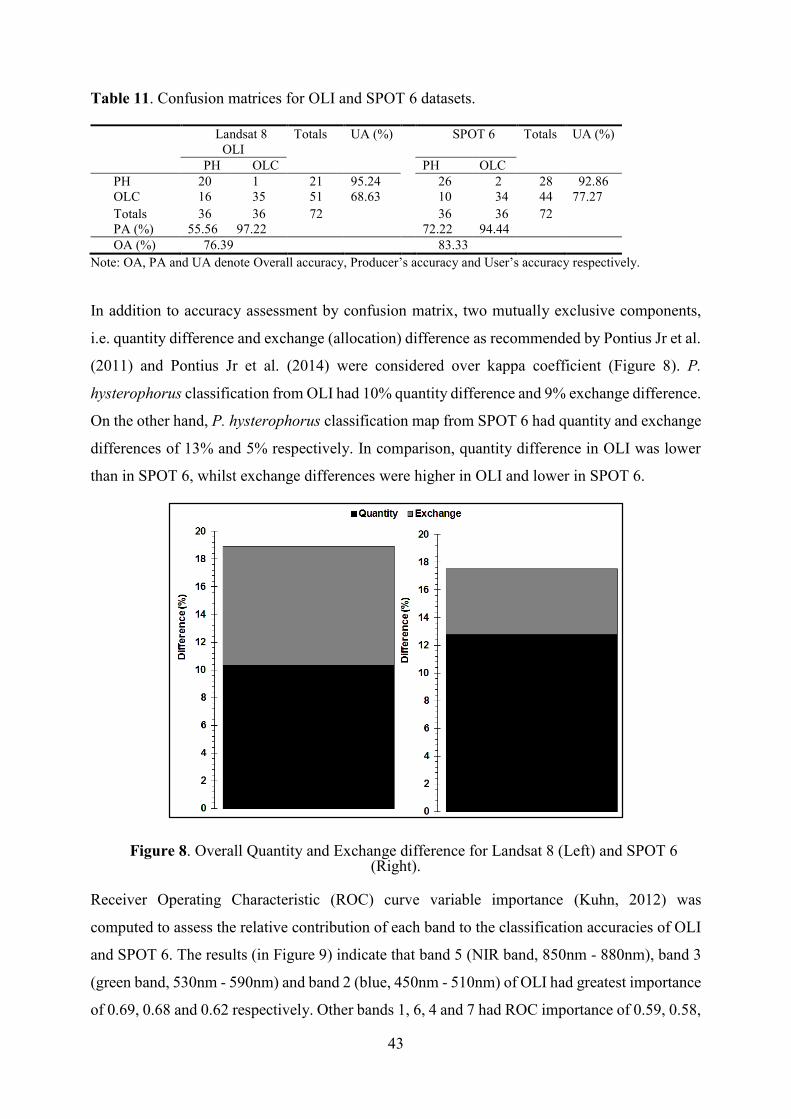
43
Table 11. Confusion matrices for OLI and SPOT 6 datasets.
Landsat 8
OLI
Totals UA (%) SPOT 6 Totals UA (%)
PH OLC PH OLC
PH 20 1 21 95.24 26 2 28 92.86
OLC 16 35 51 68.63 10 34 44 77.27
Totals 36 36 72 36 36 72
PA (%) 55.56 97.22 72.22 94.44
OA (%) 76.39 83.33
Note: OA, PA and UA denote Overall accuracy, Producer’s accuracy and User’s accuracy respectively.
In addition to accuracy assessment by confusion matrix, two mutually exclusive components,
i.e. quantity difference and exchange (allocation) difference as recommended by Pontius Jr et al.
(2011) and Pontius Jr et al. (2014) were considered over kappa coefficient (Figure 8). P.
hysterophorus classification from OLI had 10% quantity difference and 9% exchange difference.
On the other hand, P. hysterophorus classification map from SPOT 6 had quantity and exchange
differences of 13% and 5% respectively. In comparison, quantity difference in OLI was lower
than in SPOT 6, whilst exchange differences were higher in OLI and lower in SPOT 6.
Figure 8. Overall Quantity and Exchange difference for Landsat 8 (Left) and SPOT 6 (Right).
Receiver Operating Characteristic (ROC) curve variable importance (Kuhn, 2012) was
computed to assess the relative contribution of each band to the classification accuracies of OLI
and SPOT 6. The results (in Figure 9) indicate that band 5 (NIR band, 850nm - 880nm), band 3
(green band, 530nm - 590nm) and band 2 (blue, 450nm - 510nm) of OLI had greatest importance
of 0.69, 0.68 and 0.62 respectively. Other bands 1, 6, 4 and 7 had ROC importance of 0.59, 0.58,
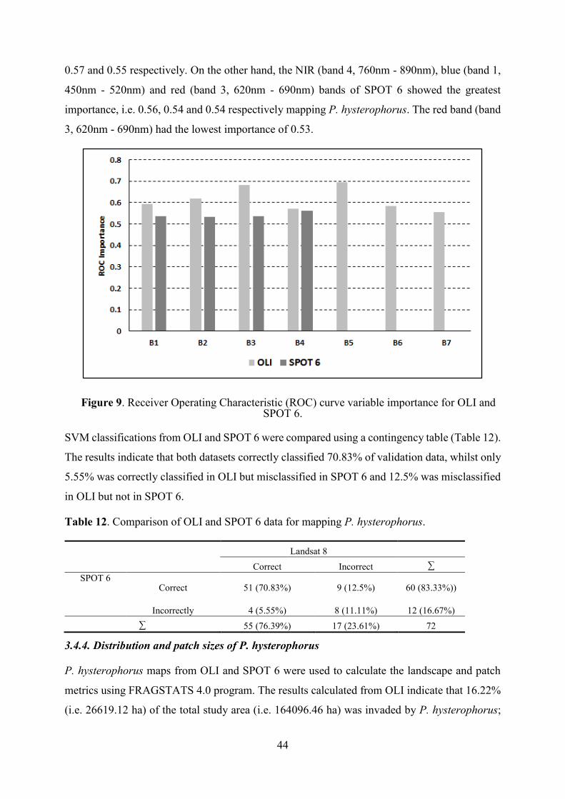
44
0.57 and 0.55 respectively. On the other hand, the NIR (band 4, 760nm - 890nm), blue (band 1,
450nm - 520nm) and red (band 3, 620nm - 690nm) bands of SPOT 6 showed the greatest
importance, i.e. 0.56, 0.54 and 0.54 respectively mapping P. hysterophorus. The red band (band
3, 620nm - 690nm) had the lowest importance of 0.53.
Figure 9. Receiver Operating Characteristic (ROC) curve variable importance for OLI and SPOT 6.
SVM classifications from OLI and SPOT 6 were compared using a contingency table (Table 12).
The results indicate that both datasets correctly classified 70.83% of validation data, whilst only
5.55% was correctly classified in OLI but misclassified in SPOT 6 and 12.5% was misclassified
in OLI but not in SPOT 6.
Table 12. Comparison of OLI and SPOT 6 data for mapping P. hysterophorus.
Landsat 8
Correct Incorrect ∑
SPOT 6 Correct 51 (70.83%) 9 (12.5%) 60 (83.33%))
Incorrectly 4 (5.55%) 8 (11.11%) 12 (16.67%)
∑ 55 (76.39%) 17 (23.61%) 72
3.4.4. Distribution and patch sizes of P. hysterophorus
P. hysterophorus maps from OLI and SPOT 6 were used to calculate the landscape and patch
metrics using FRAGSTATS 4.0 program. The results calculated from OLI indicate that 16.22%
(i.e. 26619.12 ha) of the total study area (i.e. 164096.46 ha) was invaded by P. hysterophorus;

45
the LPI was 0.26%, NumPatches was 29 607 and patch density was 18.04 patches per 100 ha.
On the other hand, the metrics calculated from SPOT 6 indicate that 6.38% (i.e. 10440.30 ha) of
the total study area (i.e. 163629.89 ha) was invaded by P. hysterophorus; the LPI was 0.15%,
NumPatches was 37 959 and patch density was 23.19 patches per 100ha. In comparison, the
metrics calculated from OLI were markedly higher than those from SPOT 6, with exception of
patch density. The results of the patch sizes calculated from OLI and SPOT 6 are presented in
Figures 10.
OLI SPOT
-50
0
50
100
150
200
250
300
350
400
450
Patc
h s
izes (
ha
)
Min-Max P. hysterophorus patches
Figure 10. P. hysterophorus patch sizes calculated from OLI and SPOT 6.
3.5. Discussions
3.5.1. The capability of multispectral data for mapping P. hysterophorus
Heritage missions such as Landsat and SPOT have a long record of remotely sensed data
covering the globe. This study exploited the capabilities of the new data from these missions for
mapping P. hysterophorus in an African savanna landscape. Despite their significant differences
in spatial resolutions, the two have visible and infrared bands which are valuable for mapping
vegetation species. Hence, have potential to characterize P. hysterophorus infestations in the
study area. The results indicated that SPOT 6 had better performance, 83.33% overall accuracy
than OLI, 76.39% (Table 13).
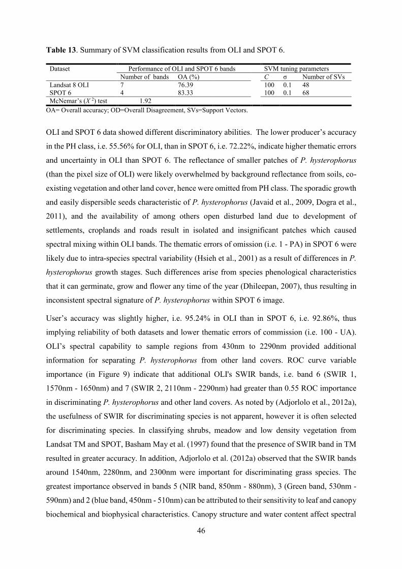
46
Table 13. Summary of SVM classification results from OLI and SPOT 6.
Dataset Performance of OLI and SPOT 6 bands SVM tuning parameters
Number of bands OA (%) C σ Number of SVs
Landsat 8 OLI 7 76.39 100 0.1 48
SPOT 6 4 83.33 100 0.1 68
McNemar’s (X 2) test 1.92
OA= Overall accuracy; OD=Overall Disagreement, SVs=Support Vectors.
OLI and SPOT 6 data showed different discriminatory abilities. The lower producer’s accuracy
in the PH class, i.e. 55.56% for OLI, than in SPOT 6, i.e. 72.22%, indicate higher thematic errors
and uncertainty in OLI than SPOT 6. The reflectance of smaller patches of P. hysterophorus
(than the pixel size of OLI) were likely overwhelmed by background reflectance from soils, co-
existing vegetation and other land cover, hence were omitted from PH class. The sporadic growth
and easily dispersible seeds characteristic of P. hysterophorus (Javaid et al., 2009, Dogra et al.,
2011), and the availability of among others open disturbed land due to development of
settlements, croplands and roads result in isolated and insignificant patches which caused
spectral mixing within OLI bands. The thematic errors of omission (i.e. 1 - PA) in SPOT 6 were
likely due to intra-species spectral variability (Hsieh et al., 2001) as a result of differences in P.
hysterophorus growth stages. Such differences arise from species phenological characteristics
that it can germinate, grow and flower any time of the year (Dhileepan, 2007), thus resulting in
inconsistent spectral signature of P. hysterophorus within SPOT 6 image.
User’s accuracy was slightly higher, i.e. 95.24% in OLI than in SPOT 6, i.e. 92.86%, thus
implying reliability of both datasets and lower thematic errors of commission (i.e. 100 - UA).
OLI’s spectral capability to sample regions from 430nm to 2290nm provided additional
information for separating P. hysterophorus from other land covers. ROC curve variable
importance (in Figure 9) indicate that additional OLI's SWIR bands, i.e. band 6 (SWIR 1,
1570nm - 1650nm) and 7 (SWIR 2, 2110nm - 2290nm) had greater than 0.55 ROC importance
in discriminating P. hysterophorus and other land covers. As noted by (Adjorlolo et al., 2012a),
the usefulness of SWIR for discriminating species is not apparent, however it is often selected
for discriminating species. In classifying shrubs, meadow and low density vegetation from
Landsat TM and SPOT, Basham May et al. (1997) found that the presence of SWIR band in TM
resulted in greater accuracy. In addition, Adjorlolo et al. (2012a) observed that the SWIR bands
around 1540nm, 2280nm, and 2300nm were important for discriminating grass species. The
greatest importance observed in bands 5 (NIR band, 850nm - 880nm), 3 (Green band, 530nm -
590nm) and 2 (blue band, 450nm - 510nm) can be attributed to their sensitivity to leaf and canopy
biochemical and biophysical characteristics. Canopy structure and water content affect spectral
47
properties in the NIR region of the electromagnetic spectrum (Schmidt and Skidmore, 2003). On
the other hand, the reflectance properties in the visible region are mainly due to pigment
concentration, chlorophyll and nitrogen content (Blackburn, 1998). OLI’s relatively narrow
bands (bandwidth less than 60nm in the visible and NIR) as compared to SPOT 6 bands (see
Table 9) also contributed to its better discriminatory ability and relatively lower commission
errors (i.e. 1 – UA). Overall the findings in this study are consistent with (Taylor et al., 2011)
who note that Landsat’s comprehensive sampling of the electromagnetic spectrum, spectral
resolution and band positioning were more important in mapping IAP’s.
Similarly, red (band 3, 620nm - 690nm) and NIR (band 4, 760nm - 890nm) bands of SPOT 6
show the greatest separability with maximum ROC importance, i.e. 0.56 and 0.53 respectively
in mapping P. hysterophorus (see Figure 5). Previous studies (Adelabu et al., 2013) observed
that red and NIR bands from Rapid-Eye data were more important than red-edge band for
mapping Colophospermum mopane and its coexisting species in a semi-arid environment. The
blue (band 1, 450 nm - 520 nm) band showed similar importance as the red band. Slightly higher
commission errors in SPOT 6 than OLI, were likely due its relatively broad bandwidths (all
greater than 60nm) which resulted into spectral overlaps between P. hysterophorus and co-
existing species. According to Taylor et al. (2011) these spectral similarities may have negative
impact on mapping accuracy. Although it was not within the scope of this study to compare the
effectiveness of classification algorithms, SVM algorithm adopted in this study showed
effectiveness in discriminating such spectral overlaps between P. hysterophorus and co-existing
species. This is evident from the observed higher number of support vectors (68) with SPOT 6
model as opposed to 48 in OLI model (see Table 13) which occurs when the classes are not
separable (Rabe et al., 2010). Results in this study are thus consistent with previous studies that
found that SVM was effective in handling complex, and non-linear class distributions (Yang et
al., 2011, Foody and Mathur, 2004). Augmented by SVM algorithm, the broader and limited
(only four) spectral bands of SPOT 6 performed better than OLI and were effective for reliably
mapping P. hysterophorus.
Overall, the results indicate that SPOT 6 had better capabilities in mapping P. hysterophorus
than OLI. The inferior overall accuracy was due to lower PA resulting from spectral mixing of
insignificant P. hysterophorus patches and other land cover. In terms of UA, OLI performed
better than SPOT 6 due to additional coastal blue and SWIR bands and narrower bandwidths as
compared to SPOT 6. Therefore, OLI’s spectral configuration was more superior to SPOT 6, and
can be used to identify the possible locations of P. hysterophorus. Related studies (Pu and

48
Landry, 2012, Fernandes et al., 2014) found that additional and strategically positioned bands of
Worldview-2 improved classification accuracy. SVM classification algorithm showed high
effectiveness in discriminating spectral overlaps of P. hysterophorus and other land covers that
occurred due to relatively broader SPOT 6 spectral bandwidths. ROC curve variable importance
from both datasets showed that visible and NIR bands were more important in mapping P.
hysterophorus. These results are consistent with (Adelabu et al., 2013, Adjorlolo et al., 2013)
who indicated that visible and NIR bands show greater discriminatory power in classifying and
mapping vegetation species.
3.5.2. Addressing information needs for optimising control mechanisms
The adverse impacts of IAP’s such as P. hysterophorus on agriculture, biodiversity, human well-
being and economy have necessitated investigations into different control and eradication
mechanisms and their effectiveness thereof (Strathie et al., 2011, Khan et al., 2012, Kumari and
Kohli, 1987). The paucity of spatial information about the distribution and patch sizes of IAP’s
hinders progress in achieving effective eradication. This study assessed the capability of OLI
and SPOT 6 in estimating the distribution and patch sizes of P. hysterophorus, valuable for
evaluating the effectiveness and optimizing control and eradication mechanisms. The
information on distribution and patch sizes is important for environmental research and
conservation planning, site specific weed management (SSWM) and for understanding
ecosystem diversity and habitat changes as a result of fragmentation by P. hysterophorus
(Franklin, 2010, Turner et al., 2003, Koller and Lanini, 2005). The distribution and patch sizes
of P. hysterophorus were calculated from OLI and SPOT 6 classification maps using
FRAGSTATS program.
Results from OLI indicated that approximately 16.22% of the study area is invaded by P.
hysterophorus, while SPOT 6 indicated that only 6% of the study area is invaded. The
discrepancies in the distributions can be attributed to significant differences in spatial resolutions
between the OLI and SPOT 6 datasets, i.e. 30m and 6m respectively. Although, minimum
mapping unit was the same for both datasets, the subsequent calculations of distribution and
patch sizes is a function of the pixel size of each dataset (He et al., 2011). OLI has a lower spatial
resolution when compared to SPOT 6, as a result it is expected that SPOT 6 will provide better
estimates of the distribution and patch sizes of P. hysterophorus. The lower spatial resolution of
OLI is inefficient of eliminating gaps inside larger P. hysterophorus patches, hence its
distribution results may be misleading. In addition, the training data for both datasets were
collected from 5m patches, hence greater generalisations can be expected in OLI than in SPOT
49
6. As a result, the overestimation of the distribution of P. hysterophorus was evident from OLI
results. On the other hand, the higher spatial resolution of SPOT 6 minimised spectral mixing
and detected isolated and insignificant patches. These discrete and insignificant P. hysterophorus
patches detected by SPOT 6 were removed by post-classification processing (which was more
effective in SPOT 6’s 6m pixels than 30m pixels of OLI), thus reducing subsequent calculations
of distribution and patch metrics.
The higher patch density, i.e. 23.19 per 100 ha in SPOT 6 and lower, i.e. 18.04 per 100 ha in
OLI is a result of the observed higher number of patches (NumPatches). With respect to
capabilities of the two datasets, the results demonstrated that SPOT 6’s spatial resolution was
more important in mapping of small patches (<0.5ha) and better delineation of patch boundaries
as compared to OLI. A similar study by (Fernandes et al., 2014) found that Worldview-2's spatial
resolution was unable to capture the boundaries of Arundo donax L. (Giant reed) in detail when
compared to airborne data. The capability to delineate boundaries and eliminate gaps inside
larger patches is desired for accurate estimation of patch sizes, since existing patches will likely
take advantage of available gaps in the landscape for their establishment and proliferation
(Malahlela et al., 2014). For invasion ecology, the results imply landscape fragmentation and
habitat loss as a result of P. hysterophorus invasion which possibly led to a replacement of native
species.
Patch size is the single most important information contained in the landscape (McGarigal et al.,
2002). An understanding of patch sizes will assist land managers to monitor changes in the
landscape and establish relationships between the invader and changes in the ecosystem and
habitats (Turner et al., 2003). Detailed visual assessment of P. hysterophorus maps from OLI
and SPOT 6 indicated that larger patches dominantly occur in communal croplands (Figure 11),
while smaller patches occur along roadsides and building peripheries. In essence, the LPI found
for both OLI, i.e. 0.26% and SPOT 6, i.e. 0.15% resulted from P. hysterophorus invasion in
cropland and overgrazed rangelands. Invasion, colonization and establishment of P.
hysterophorus in the study area can be attributed to landscape and habitat disturbance due to
human travel corridors, development of settlements and farming practices. The largest patches
in the landscape indicate successful colonization by P. hysterophorus, thus the results from OLI
imply greater establishment and dominance of the species than those from SPOT 6. Such largest
patches in the landscape, usually occurring in croplands and overgrazed grassland, imply a
decrease in productivity and extent of communal agricultural lands and appropriates the
opportunity of overgrazed lands to recover. On the other hand, patch sizes results (Figure 10)

50
indicated that most patches calculated from both OLI and SPOT 6 were less than 15 ha. Smaller
patches demonstrate new introductions, thus it may be beneficial to target such patches for
control and eradication purposes. On the other hand, larger patches can be targeted for
containment to prevent further spread. In consistency with the marked differences, i.e. 10.22%
observed in the distributions of the P. hysterophorus calculated from OLI and SPOT 6. Mann-
Whiney U test indicated that there is significant differences in patch sizes calculated from the
two datasets at P < 0.05. The differences emanates from overestimations by OLI pixels.
Figure 11. SPOT 6 patch sizes in communal croplands overlaid on aerial image acquired in 2009/10 and picture on the right represents the respective infested areas as seen in the field in
February 2014.
Overall, the distribution and patch sizes from OLI were higher than those calculated from SPOT
6. Both datasets demonstrate a potential in providing essential information for control and
management of P. hysterophorus. OLI’s relatively larger pixels would be suitable for
characterizing well-established, larger patches occurring in croplands and overgrazed rangelands
useful for large scale detection and monitoring. As a result, the distribution and patch sizes
calculated from OLI for small patches may be misleading. On the other hand, SPOT 6 is suitable
for delineating gaps and boundaries of smaller patches useful for site-specific weed management.

51
3.6. Conclusions
This chapter evaluated the capability of medium resolution multispectral data from Landsat 8
OLI and relatively high resolution SPOT 6 for reliably mapping the distribution and patch sizes
of P. hysterophorus using SVM classifier. In conclusion, OLI’s comprehensive spectral
sampling from 430nm to 2290nm, spectral resolution, and number of bands were important for
reliably separating P. hysterophorus and other land cover types. However, spectral mixing due
to larger pixel size limited its capability (i.e. inferior overall accuracy) to provide reliable
distribution and patch sizes information. In addition, OLI’s larger pixels resulted in
overestimations of the distributions and patch sizes, hence may be suitable for mapping well-
established patches for large scale monitoring. Although this study did not compare algorithms,
SVM showed effectiveness in discriminating spectral overlaps of P. hysterophorus and other
land covers within SPOT 6 bands. On the other hand, SPOT 6’s 6m resolution showed better
estimations of distributions and delineating gaps and boundaries in P. hysterophorus patches.
Ecologically, the distribution and patch sizes calculated from OLI and SPOT 6 showed higher
fragmentation of the landscape, habitat loss and decrease in productive land due to P.
hysterophorus invasion. As a result, small patches can be prioritised for eradication, while larger
patches can be contained to prevent further spread.
Overall, the study demonstrated the potential of medium resolution data from OLI and relatively
high resolution SPOT 6 in providing useful information necessary for effective land
management, site specific weed management, and site prioritisation in conservation plans.
Therefore this study provide the basis towards an IAP species detection and monitoring system
to identify and target both small and large patches for control and eradication.

52
CHAPTER 4
SYNTHESIS AND CONCLUSION
4.1. Introduction
In the savanna landscapes of northern Kwa Zulu Natal, P. hysterophorus has reached epidemic
proportions, thus posing a threat to biodiversity, agriculture, ecosystem functioning and services
and human well-being. The physiological characteristics of P. hysterophorus, in its vegetative
and mature growth stages are dominated by creamy-white flowers. These are produced in only
four to six weeks after germination, followed by the production of approximately 25 000 easily
dispersible seeds per plant (Dogra et al., 2011). The characteristics of P. hysterophorus during
vegetative and mature growing stages support its prolific spread and sporadic growth, making it
extremely difficult to contain and eradicate. As a result, the effectiveness of physical, chemical
and biological control mechanisms is increased during the juvenile growing stage (Reddy et al.,
2009, Khan et al., 2012). Thus, for early detection and optimization of eradication mechanisms,
it becomes essential to explore the potential of hyperspectral and multispectral remote sensing
data for discriminating and mapping P. hysterophorus. Conventional methods such as field
surveys and manual digitising are laborious, time consuming, costly, and inappropriate for large
and inaccessible areas.
The results in this study showed the potential of remote sensing for discriminating and mapping
a problematic IAP’s, P. hysterophorus. Specifically, the study demonstrated the capabilities of
canopy hyperspectral data in discriminating P. hysterophorus against its co-existing species. A
novel approach for overcoming Hughes effect and to select relevant combination of spectral
bands that improve accuracy has been proposed. The results were significant for understanding
the underlying inter-species spectral differences, and identifying optimal bands valuable for
operational mapping using airborne and satellite sensors, choosing suitable sensor for mapping
and early IAP species detection (Chapter 2). Based on the identified bands, accessible
multispectral data were chosen, i.e. OLI and SPOT 6 and the capability for providing the spatial
distribution and patch sizes of P. hysterophorus was pursued. The results demonstrated the
potential of the spectral and spatial configurations of OLI and SPOT 6 for reliably mapping the
distribution and patch sizes of P. hysterophorus (Chapter 3). The information about the spatial
distribution and patch sizes of P. hysterophorus is critical for identifying new infestations,
optimizing control mechanisms, and effective land management and conservation planning.

53
4.2. Improving classification accuracy through feature subset selection and
dimensionality reduction
The inherent high dimensionality characteristic of hyperspectral data has been identified as the
major limitation in literature (Adam and Mutanga, 2009, Adjorlolo et al., 2013). Large training
samples (n > 100 per class) are required in order to obtain better accuracies. However, in reality,
it is costly, tedious and time consuming to collect large samples (Adam and Mutanga, 2009). As
a result, reliable discrimination of species with hyperspectral data is compromised due to the
effect of n < p (Hughes, 1968). Therefore, selection of a smaller subset of bands that capture the
properties of the entire dataset has become a prerequisite for computational efficiency and
reliable classification accuracy (Zhang and Ma, 2009, Pal and Foody, 2010, Löw et al., 2013).
An innovative hierarchical approach integrating statistical significant tests, inter-band
correlation and variable importance, and SVM-RFE was proposed in Chapter 2. In comparison
with entire spectral dataset (n = 1633) and a combination of 20 best spectral bands selected by
SVM-RFEE, the proposed approach showed that a small subset of spectral bands, n = 10 was
significant for reliable discrimination of P. hysterophorus and co-existing species. In addition,
the hierarchical approach systematically reduced dimensionality and collinearity, hence the
selected subset can be used with usually preferred conventional classifiers such as Maximum
Likelihood. This is because the selected spectral bands retained important discriminative
properties of the entire dataset.
Important findings regarding the significance of feature selection and dimensionality reduction
in improving classification accuracy (as highlighted in Chapter 2) are:
1. SVM classification training time and accuracy improved when using 10 spectral bands
selected by the proposed hierarchical approach, than when using entire spectral
dataset and SVM-RFE.
2. The lower SVM classification accuracy with entire spectral data demonstrate the
effect of “curse of dimensionality” on SVM performance, hence higher classification
accuracy obtained with the hierarchical approach demonstrate the need for feature
selection and dimensionality reduction even when using powerful algorithms.
These findings are valuable for operational discrimination and mapping of P. hysterophorus in
its early growth stage using airborne and satellite hyperspectral sensors, thus may aid effective
control and eradication the species.

54
4.3. Optimal spectral bands for discrimination of P. hysterophorus
Canopy hyperspectral data provide an important starting point for in-depth understanding of
species spectral properties prior mapping. The differences in reflectance properties between
species are a representation of their differences in canopy and leaf biochemical and biophysical
properties (see Figure 12).
Figure 12. Canopy and leaf structures and spectral signatures of P. hysterophorus (PH), Acacia Trees (AT), Grass species (GS) and Other plant species (OPS).
Inter-species differences in reflectance properties facilitate species discrimination (Adam and
Mutanga, 2009, Chun et al., 2011), however, only few and specific spectral bands with high
discriminative ability between all species-pairs are desired. An innovative hierarchical approach
that integrates statistical filters (Kruskal Wallis ANOVA, Inter-band correlation and AUC-ROC
variable importance) and wrapper-based technique (SVM-RFE) was proposed to select a
minimum but optimal subset of spectral bands that capture relevant properties of the entire
dataset. At each stage of analysis, the useful spectral bands offering greatest capability for
discriminating all species-pairs were determined.
Specifically, Kruskall-Wallis ANOVA identified 599 spectral bands in all regions of the
electromagnetic spectrum that are statistically significant and have greater separability for P.
hysterophorus and its co-species. Subsequently, inter-band correlation and variable importance
identified 14 spectral bands that are less redundant and have high individual discriminative
ability in distinguishing P. hysterophorus from its co-species. Up to this stage, the identified
spectral bands are essential for operational applications with conventional classifiers such as

55
Maximum Likelihood. SVM-RFE selected the final and optimal subset of spectral bands (n =
10) that consisted of two red-edge bands located at 685nm and 707nm, one NIR band located at
1115nm and seven SWIR bands at 1971nm, 1982nm, 1966nm, 2003nm, 2013nm and 2005nm.
The usefulness of red-edge, NIR and SWIR regions for discriminating species has been reported
in literature (Schmidt and Skidmore, 2003, Mutanga and Skidmore, 2007, Adam and Mutanga,
2009). In addition, all selected spectral bands (in this study) were different from those selected
in other recent studies (see Table 14), reinforcing the assertion that there is no single technique
useful for all species types.

56
Table 14. Previously selected bands for species discrimination separated by broad spectral
regions suggested by (Fernandes et al., 2013).
Spectral
regions
Reference Selected band (s) Species
350 – 449nm
(Blue)
This study 0 P. hysterophorus
(Jia et al., 2011) 405nm, 424nm, 438 nm Opium poppy
(Adam and Mutanga, 2009) 0 Cyperus papyrus
450 – 549nm
(Green)
This study 0 P. hysterophorus
(Jia et al., 2011) 468nm, 524nm, 528nm Opium poppy
(Adam and Mutanga, 2009) 0 Cyperus papyrus
550 – 649nm
(Red)
This study 0 P. hysterophorus
(Jia et al., 2011) 0 Opium poppy
(Adam and Mutanga, 2009) 0 Cyperus papyrus
650 – 749nm
(Red-edge)
This study 685nm, 707nm P. hysterophorus
(Jia et al., 2011) 726nm, 736nm, 746nm, Opium poppy
(Adam and Mutanga, 2009) 745nm, 746nm Cyperus papyrus
750 –
1299nm
(NIR)
This study 1115nm P. hysterophorus
(Jia et al., 2011) 754nm, 760nm, 982nm,1207nm,
1220nm
Opium poppy
(Adam and Mutanga, 2009) 892nm, 932nm, 934nm, 958nm,
961nm, 989nm
Cyperus papyrus
1300 –
2500nm
(SWIR)
This study 1971nm, 1982nm, 1990nm,
1966nm, 2003nm, 2013nm,
2005nm
P. hysterophorus
(Jia et al., 2011) 1974nm, 1689nm Opium poppy
(Adam and Mutanga, 2009) 0 Cyperus papyrus
An important finding in Chapter 2 regarding optimal spectral bands for discrimination of P.
hysterophorus and co-existing species was that:
1. The identified fewer spectral bands by the hierarchical approach, n = 10 have greatest
potential for discriminating P. hysterophorus using current and next generation airborne
and satellite hyperspectral sensors. Considering the harmful impacts of P.
hysterophorus, the selected spectral bands can be used as a guidance for choosing

57
appropriate bands for detection and mapping of the distribution and patches of the
species.
4.4. Reliable information for effective management of P. hysterophorus
The spectral discrimination analysis in Chapter 2 identified 10 spectral bands for reliably
discriminating P. hysterophorus and its co-existing species using canopy hyperspectral data. The
optimal bands were located in the red edge (685nm, 707nm), NIR (1115nm) and SWIR (1971nm,
1982nm, 1990nm, 1966nm, 2003nm, 2013nm, 2005nm) regions of the electromagnetic
spectrum. As part of the analysis (in Chapter 2), inter-band correlation and variable importance
identified other important bands located in blue (427nm), green (537nm) and red (562nm)
regions. However, the identified bands do not fully coincide with the bands in most accessible
multispectral data. In addition, there was no hyperspectral image available that covers the study
area. In that regard, in order to address the challenges of the lack of information on the
distribution and patch sizes, we assessed the capability of multispectral data from heritage
missions, i.e. Landsat and SPOT. The advantage of the data from these missions is that they have
long record of data useful for understanding historical spread of IAP species, are sustainable, the
datasets are compatible and contain necessary spectral bands for mapping plant species (Adelabu
et al., 2013, Adjorlolo et al., 2013). The usefulness of the spatial and spectral configurations of
these datasets have never, to the best of our knowledge, been explored. As such, we compared
the capability of OLI and SPOT 6 for mapping the distribution and patch sizes of P.
hysterophorus.
Important findings in the study (Chapter 3) were:
1. The higher spatial resolution in SPOT 6 was useful for better characterization of the
distribution and patch sizes, while the spectral configuration in OLI was more important
in identifying possible locations infested by P. hysterophorus.
2. The landscape and patch metrics calculated from OLI were markedly different from
those calculated from SPOT 6 due to differences in resolution. This was due to the
inefficiency of OLI’s larger pixels in eliminating gaps inside larger P. hysterophorus
patches, while SPOT 6’s relatively smaller pixels minimised spectral mixing, and
detected isolated and insignificant patches.
Results from this study (Chapter 3) provide a basis for understanding the ecological relationships
between invasion of P. hysterophorus and changes in ecosystems and habitats (Turner et al.,
2003). The capability to eliminate gaps by SPOT 6 is desirable since the existing P.

58
hysterophorus patches will likely target such gaps in the landscape for their establishment and
proliferation (Malahlela et al., 2014). In addition, landscape and patch metrics from both datasets
suggests intense fragmentation and habitat loss as a result of P. hysterophorus invasion.
Therefore, these findings are critical for allocation of resources for controlling and eradicating
P. hysterophorus and effective land management and conservation planning (see Appendix B)
4.5. Conclusions and Recommendations
The aim of this study was to evaluate the capability of hyperspectral and multispectral data for
mapping problematic IAP’s, P. hysterophorus in the northern Kwa Zulu Natal province, South
Africa. It is clear from the findings in this dissertation that canopy hyperspectral data was useful
in identifying optimal spectral bands from highly dimensional data for discriminating P.
hysterophorus and co-existing species. In addition, the findings determined the potential of
widely accessible multispectral data from heritage missions (i.e. Landsat and SPOT) for
addressing the lack of information about the spatial distributions and patch sizes of P.
hysterophorus. Up-to-date and accurate information about the distribution and patch sizes of P.
hysterophorus is critical for understanding its spatial and structural variability in the landscape.
Also, the distribution and patch sizes maps may aid proper planning and allocation of resources,
hence useful for site-specific weed management.
The overall conclusions based on the objectives of this study as addressed in Chapter 2 and 3 are
as follows:
1. There is no single technique that has been proven superior in reducing dimensionality in
hyperspectral data (Yang et al., 2005) and identifying smaller subset of bands that
capture properties of the entire dataset (Adam and Mutanga, 2009, Pal and Foody, 2010,
Jia et al., 2011). The potential of an innovative hierarchical approach that integrates
statistical analysis and wrapper-based approach has been demonstrated. Ten
hierarchically selected spectral bands had better performance in classifying P.
hysterophorus and co-existing species when compared to entire spectral dataset and a
combination of 20 spectral bands selected by SVM-RFE.
2. In consistency with previous studies (Zhang and Ma, 2009, Pal and Foody, 2010), this
study found that SVM classifier was affected by Hughes effect when applied to entire
spectral dataset.
3. Previous studies observed that SVM-RFE performs better when feature space is limited
<12 bands (Zhang and Ma, 2009, Pal and Foody, 2010). Statistical filters prior to SVM-

59
RFE were useful for identifying bands with high statistical separability and importance
(n = 14), hence optimized its performance when applied within the Hierarchical
approach.
4. The higher spatial resolution of SPOT 6 offer the potential to provide up-to-date and
accurate information on spatial distributions and patch sizes of P. hysterophorus,
valuable for eradication resource allocation, effective land management and
conservation planning.
5. On the other hand, OLI’s comprehensive spectral sampling from 430nm – 2291nm,
relatively higher spectral resolution and band positioning can be used for locating larger
patches of P. hysterophorus, valuable for areas where the species is widely spread.
The major limitations of the study emanated from the lower quality of training data, hence
resulted in lower classification accuracy for OLI. As such, future studies should focus on
improving the quality of training and validation data, and explore the utility of vegetation indices
in addition to bands in mapping P. hysterophorus. Since OLI offered better spectral configuration
and SPOT 6 better spatial configuration, the two datasets can be combined in multiresolution or
multiscale classification model to produce higher classification accuracy and better elimination
of gaps and well-defined patch boundaries. Also, up-scaling to space-borne hyperspectral data
based on the future sensors such as EnMap, should be explored.

60
REFERENCES
ADAM, E. & MUTANGA, O. 2009. Spectral discrimination of papyrus vegetation (Cyperus
papyrus L.) in swamp wetlands using field spectrometry. ISPRS Journal of
Photogrammetry and Remote Sensing, 64, 612-620.
ADAM, E., MUTANGA, O. & RUGEGE, D. 2010. Multispectral and hyperspectral remote
sensing for identification and mapping of wetland vegetation: a review. Wetlands
Ecology and Management, 18, 281-296.
ADELABU, S., MUTANGA, O., ADAM, E. & CHO, M. A. 2013. Exploiting machine
learning algorithms for tree species classification in a semiarid woodland using
RapidEye image. Journal of Applied Remote Sensing, 7, 073480-073480.
ADJORLOLO, C., CHO, M. A., MUTANGA, O. & ISMAIL, R. 2012a. Optimizing spectral
resolutions for the classification of C3 and C4 grass species, using wavelengths of
known absorption features. Journal of Applied Remote Sensing, 6, 063560-1-063560-
15.
ADJORLOLO, C., MUTANGA, O., CHO, M. & ISMAIL, R. 2012b. Challenges and
opportunities in the use of remote sensing for C3 and C4 grass species discrimination
and mapping. African Journal of Range & Forage Science, 29, 47-61.
ADJORLOLO, C., MUTANGA, O., CHO, M. A. & ISMAIL, R. 2013. Spectral resampling
based on user-defined inter-band correlation filter: C 3 and C 4 grass species
classification. International Journal of Applied Earth Observation and Geoinformation,
21, 535-544.
ADKINS, S. & SHABBIR, A. 2014. Biology, ecology and management of the invasive
parthenium weed (Parthenium hysterophorus L.). Pest management science, 70, 1023-
1029.
ARZANDEH, S. & WANG, J. 2003. Monitoring the change of Phragmites distribution using
satellite data. Canadian Journal of Remote Sensing, 29, 24-35.
ATKINSON, J. T., ISMAIL, R. & ROBERTSON, M. 2014. Mapping bugweed (solanum
mauritianum) infestations in pinus patula plantations using hyperspectral imagery and
support vector machines. IEEE Journal of Selected Topics in Applied Earth
Observations and Remote Sensing, 7, 17-28.

61
ATKINSON, P. M. & TATNALL, A. 1997. Introduction neural networks in remote sensing.
International Journal of Remote Sensing, 18, 699-709.
BAJWA, S., MISHRA, A. & NORMAN, R. 2010. Canopy reflectance response to plant
nitrogen accumulation in rice. Precision agriculture, 11, 488-506.
BASHAM MAY, A. M., PINDER III, J. & KROH, G. 1997. A comparison of LANDSAT
Thematic Mapper and SPOT multi-spectral imagery for the classification of shrub and
meadow vegetation in Northern California, USA. International Journal of Remote
Sensing, 18, 3719-3728.
BELZ, R. G., REINHARDT, C. F., FOXCROFT, L. C. & HURLE, K. 2007. Residue
allelopathy in Parthenium hysterophorus L.—Does parthenin play a leading role? Crop
Protection, 26, 237-245.
BLACKBURN, G. A. 1998. Quantifying chlorophylls and caroteniods at leaf and canopy
scales: An evaluation of some hyperspectral approaches. Remote Sensing of
Environment, 66, 273-285.
BOSER, B. E., GUYON, I. M. & VAPNIK, V. N. A training algorithm for optimal margin
classifiers. Proceedings of the fifth annual workshop on Computational learning
theory, 1992. ACM, 144-152.
BRADLEY, B. A. & MUSTARD, J. F. 2005. Identifying land cover variability distinct from
land cover change: cheatgrass in the Great Basin. Remote Sensing of Environment, 94,
204-213.
BREIMAN, L. 2001. Random forests. Machine learning, 45, 5-32.
BUCKINGHAM, R. & STAENZ, K. 2008. Review of current and planned civilian space
hyperspectral sensors for EO. Canadian Journal of Remote Sensing, 34, S187-S197.
BURGES, C. J. 1998. A tutorial on support vector machines for pattern recognition. Data
mining and knowledge discovery, 2, 121-167.
CAMPS-VALLS, G. & BRUZZONE, L. 2005. Kernel-based methods for hyperspectral image
classification. IEEE Transactions on Geoscience and Remote Sensing, 43, 1351-1362.
CARPENTER, G., GJAJA, M. N., GOPAL, S. & WOODCOCK, C. E. 1997. ART neural
networks for remote sensing: vegetation classification from Landsat TM and terrain
data. IEEE Transactions on Geoscience and Remote Sensing, 35, 308-325.
CARTER, G. A. 1994. Ratios of leaf reflectances in narrow wavebands as indicators of plant
stress. Remote Sensing, 15, 697-703.

62
CHI, M., FENG, R. & BRUZZONE, L. 2008. Classification of hyperspectral remote-sensing
data with primal SVM for small-sized training dataset problem. Advances in Space
Research, 41, 1793-1799.
CHO, M. A., DEBBA, P., MUTANGA, O., DUDENI-TLHONE, N., MAGADLA, T. &
KHULUSE, S. A. 2012. Potential utility of the spectral red-edge region of
SumbandilaSat imagery for assessing indigenous forest structure and health.
International journal of applied earth observation and Geoinformation, 16, 85-93.
CHO, M. A., MALAHLELA, O. & RAMOELO, A. 2015. Assessing the utility WorldView-2
imagery for tree species mapping in South African subtropical humid forest and the
conservation implications: Dukuduku forest patch as case study. International Journal
of Applied Earth Observation and Geoinformation, 38, 349-357.
CHUN, B. B., JAFRI, M. Z. M. & SAN, L. H. Reflectance characteristic of certain mangrove
species at Matang Mangrove Forest Reserve, Malaysia. IEEE International Conference
on Space Science and Communication (IconSpace), 2011 2011. IEEE, 147-151.
CHUN, H. & KELEŞ, S. 2010. Sparse partial least squares regression for simultaneous
dimension reduction and variable selection. Journal of the Royal Statistical Society:
Series B (Statistical Methodology), 72, 3-25.
CLARK, R. N. & ROUSH, T. L. 1984. Reflectance spectroscopy: Quantitative analysis
techniques for remote sensing applications. Journal of Geophysical Research: Solid
Earth (1978–2012), 89, 6329-6340.
CLEVERS, J., VAN DER HEIJDEN, G., VERZAKOV, S. & SCHAEPMAN, M. 2007.
Estimating grassland biomass using SVM band shaving of hyperspectral data.
Photogrammetric Engineering & Remote Sensing, 73, 1141-1148.
CONGALTON, R. G. 1991. A review of assessing the accuracy of classifications of remotely
sensed data. Remote Sensing of Environment, 37, 35-46.
COOLEY, T., ANDERSON, G., FELDE, G., HOKE, M., RATKOWSKI, A., CHETWYND,
J., GARDNER, J., ADLER-GOLDEN, S., MATTHEW, M. & BERK, A. FLAASH, a
MODTRAN4-based atmospheric correction algorithm, its application and validation.
IEEE International Geoscience and Remote Sensing Symposium, 2002. IGARSS'02.
2002 2002. IEEE, 1414-1418.
CORTES, C. & VAPNIK, V. 1995. Support-vector networks. Machine Learning, 20, 273-297.
CURRAN, P. J. 2001. Imaging spectrometry for ecological applications. International Journal
of Applied Earth Observation and Geoinformation, 3, 305-312.

63
DARVISHZADEH, R., SKIDMORE, A., SCHLERF, M., ATZBERGER, C., CORSI, F. &
CHO, M. 2008. LAI and chlorophyll estimation for a heterogeneous grassland using
hyperspectral measurements. ISPRS Journal of Photogrammetry and Remote Sensing,
63, 409-426.
DAUGHTRY, C., WALTHALL, C., KIM, M., DE COLSTOUN, E. B. & MCMURTREY, J.
2000. Estimating corn leaf chlorophyll concentration from leaf and canopy reflectance.
Remote Sensing of Environment, 74, 229-239.
DE JONG, S. M., ADDINK, E. A. & DOELMAN, J. C. 2014. Detecting leaf-water content in
Mediterranean trees using high-resolution spectrometry. International Journal of
Applied Earth Observation and Geoinformation, 27, 128-136.
DEMIR, B. & ERTÜRK, S. 2008. Phase correlation based redundancy removal in feature
weighting band selection for hyperspectral images. International journal of Remote
sensing, 29, 1801-1807.
DENG, S., XU, Y., LI, L., LI, X. & HE, Y. 2013. A feature-selection algorithm based on
support vector machine-multiclass for hyperspectral visible spectral analysis. Journal of
Food Engineering, 119, 159-166.
DHILEEPAN, K. 2007. Biological control of parthenium (Parthenium hysterophorus) in
Australian rangeland translates to improved grass production. Weed Science, 55, 497-
501.
DHILEEPAN, K. & MCFADYEN, R. C. 2012. Parthenium hysterophorus L.–parthenium.
Biological control of weeds in Australia. CSIRO, Melbourne, 448-462.
DIELEMAN, J. & MORTENSEN, D. 1999. Characterizing the spatial pattern. Weed research,
39.
DOGRA, K., KOHLI, R. & SOOD, S. 2009. An assessment and impact of three invasive
species in the Shivalik hills of Himachal Pradesh, India. International Journal of
Biodiversity and Conservation, 1, 004-010.
DOGRA, K. S., SOOD, S. K., DOBHAL, P. K. & SHARMA, S. 2010. Alien plant invasion
and their impact on indigenous species diversity at global scale: A review. Journal of
ecology and the natural environment, 2, 175-186.
DOGRA, K. S., SOOD, S. K. & SHARMA, R. 2011. Distribution, Biology and Ecology of
Parthenium hysterophorus L.(Congress Grass) an invasive species in the North-Western
Indian Himalaya (Himachal Pradesh). African Journal of Plant Science, 5, 682-687.
DOGRA, K. S., SOOD, K.S. AND SHARMA, R. 2011. Distribution, Biology and Ecology of
Parthenium hysterophorus L. (Congress Grass) an invasive species in the North-

64
Western Indian Himalaya (Himachal Pradesh). African Journal of Plant Science, 5,
682-687.
DORIGO, W., LUCIEER, A., PODOBNIKAR, T. & ČARNI, A. 2012. Mapping invasive
Fallopia japonica by combined spectral, spatial, and temporal analysis of digital
orthophotos. International Journal of Applied Earth Observation and Geoinformation,
19, 185-195.
DORIGO, W., LUCIEER, A., PODOBNIKAR, T. & CARNI, A. 2012. Mapping invasive
Fallopia japonica by combined spectral, spatial, and temporal analysis of digital
orthophotos. International Journal of Applied Earth Observation and Geoinformation,
19, 185-195.
DUNN, O. J. 1964. Multiple comparisons using rank sums. Technometrics, 6, 241-252.
EVERITT, J. & JUDD, F. 1989. Using remote sensing techniques to distinguish and monitor
black mangrove (Avicennia germinans). Journal of Coastal Research, 737-745.
EVERITT, J. H., YANG, C. & DELOACH, C. 2005. Remote sensing of giant reed with
QuickBird satellite imagery. Journal of Aquatic Plant Management, 43, 81-85.
FAURTYOT, T. & BARET, F. 1997. Vegetation water and dry matter contents estimated from
top-of-the-atmosphere reflectance data: a simulation study. Remote Sensing of
Environment, 61, 34-45.
FERNANDES, M. R., AGUIAR, F. C., SILVA, J. M., FERREIRA, M. T. & PEREIRA, J. M.
2013. Spectral discrimination of giant reed (Arundo donax L.): A seasonal study in
riparian areas. ISPRS Journal of Photogrammetry and Remote Sensing, 80, 80-90.
FERNANDES, M. R., AGUIAR, F. C., SILVA, J. M., FERREIRA, M. T. & PEREIRA, J. M.
2014. Optimal attributes for the object based detection of giant reed in riparian habitats:
A comparative study between Airborne High Spatial Resolution and WorldView-2
imagery. International Journal of Applied Earth Observation and Geoinformation, 32,
79-91.
FOODY, G. M. 2002. Status of land cover classification accuracy assessment. Remote sensing
of environment, 80, 185-201.
FOODY, G. M. & MATHUR, A. 2004. A relative evaluation of multiclass image classification
by support vector machines. IEEE Transactions on Geoscience and Remote Sensing,
42, 1335-1343.
FRANKLIN, J. 2010. Mapping species distributions: spatial inference and prediction,
Cambridge University Press.

65
FRAZIER, A. & WANG, L. 2011. Characterizing spatial patterns of invasive species using
sub-pixel classifications. Remote Sensing of Environment, 115, 1997-2007.
GAMON, J., SERRANO, L. & SURFUS, J. 1997. The photochemical reflectance index: an
optical indicator of photosynthetic radiation use efficiency across species, functional
types, and nutrient levels. Oecologia, 112, 492-501.
GARDNER, J. L. 2003. Uncertainties in interpolated spectral data. Journal of Research-
National Institute of Standards and Technology, 108, 69-78.
GAVIER-PIZARRO, G. I., KUEMMERLE, T., HOYOS, L. E., STEWART, S. I., HUEBNER,
C. D., KEULER, N. S. & RADELOFF, V. C. 2012. Monitoring the invasion of an
exotic tree (Ligustrum lucidum) from 1983 to 2006 with Landsat TM/ETM+ satellite
data and Support Vector Machines in Córdoba, Argentina. Remote Sensing of
Environment, 122, 134-145.
GUYON, I. & ELISSEEFF, A. 2006. An introduction to feature extraction. Feature Extraction.
Springer.
GUYON, I., WESTON, J., BARNHILL, S. & VAPNIK, V. 2002. Gene selection for cancer
classification using support vector machines. Machine learning, 46, 389-422.
HE, K. S., ROCCHINI, D., NETELER, M. & NAGENDRA, H. 2011. Benefits of
hyperspectral remote sensing for tracking plant invasions. Diversity and Distributions,
17, 381-392.
HEIJTING, S., VAN DER WERF, W., STEIN, A. & KROPFF, M. 2007. Are weed patches
stable in location? Application of an explicitly two‐dimensional methodology. Weed
Research, 47, 381-395.
HENDERSON, L. 1999. The Southern African Plant Invaders Atlas (SAPIA) and its
contribution to biological weed control. African Entomology, 1, 159-163.
HSIEH, P.-F., LEE, L. C. & CHEN, N.-Y. 2001. Effect of spatial resolution on classification
errors of pure and mixed pixels in remote sensing. IEEE Transactions on Geoscience
and Remote Sensing, 39, 2657-2663.
HSU, C.-W., CHANG, C.-C. & LIN, C.-J. 2003. A practical guide to support vector
classification.
HSU, C.-W. & LIN, C.-J. 2002. A comparison of methods for multiclass support vector
machines. IEEE Transactions on Neural Networks, 13, 415-425.
HUANG, C.-Y. & ASNER, G. P. 2009. Applications of remote sensing to alien invasive plant
studies. Sensors, 9, 4869-4889.

66
HUANG, C., GEIGER, E., VAN LEEUWEN, W. & MARSH, S. 2009. Discrimination of
invaded and native species sites in a semi‐desert grassland using MODIS multi‐
temporal data. International Journal of Remote Sensing, 30, 897-917.
HUANG, Z., TURNER, B. J., DURY, S. J., WALLIS, I. R. & FOLEY, W. J. 2004. Estimating
foliage nitrogen concentration from HYMAP data using continuum removal analysis.
Remote Sensing of Environment, 93, 18-29.
HUGHES, G. 1968. On the mean accuracy of statistical pattern recognizers. IEEE
Transactions on Information Theory, 14, 55-63.
JANZ, A., VAN DER LINDEN, S., WASKE, B. AND HOSTER, P. 2007. imageSVM - A
user-Oriented Tool for Advanced Classification of Hyperspectral Data Uisng Support
Vector Machines. Proceedings 5th EARSel Workshop on Imaging Spectroscopy, 23-
25 April 2007 2007 Bruges, Belgium. EARSel, 1-5.
JAVAID, A., SHAFIQUE, S. & SHAFIQUE, S. 2009. Invasion of noxious alien weed
Parthenium hysterophorus L. in grazing lands of Lahore, Pakistan. Journal of Animal
and Plant Sciences, 19, 149-153.
JENSEN, J. R. 1983. Biophysical remote sensing. Annals of the Association of American
Geographers, 73, 111-132.
JENSEN, R., MAUSEL, P., DIAP’S, N., GONSER, R., YANG, C., EVERITT, J. &
FLETCHER, R. 2007. Spectral analysis of coastal vegetation and land cover using
AISA+ hyperspectral data. Geocarto International, 22, 17-28.
JIA, K., WU, B., TIAN, Y., LI, Q. & DU, X. 2011. Spectral discrimination of opium poppy
using field spectrometry. IEEE Transactions on Geoscience and Remote Sensing, 49,
3414-3422.
JOE, H. 1990. Multivariate concordance. Journal of multivariate analysis, 35, 12-30.
KANDWAL, R., JEGANATHAN, C., TOLPEKIN, V. & KUSHWAHA, S. 2009.
Discriminating the invasive species,‘Lantana’using vegetation indices. Journal of the
Indian Society of Remote Sensing, 37, 275-290.
KARATZOGLOU, A., MEYER, D. & HORNIK, K. 2005. Support vector machines in R.
Research Report Series/Department of Statistics and Mathematics, 21.
KARATZOGLOU, A., SMOLA, A., HORNIK, K. & ZEILEIS, A. 2004. kernlab-an S4
package for kernel methods in R. Journal of Statistical Software, 11.
KAYA, G. T. 2013. A hybrid model for classification of remote sensing images with linear
SVM and support vector selection and adaptation. IEEE Journal of Selected Topics in
Applied Earth Observations and Remote Sensing, 6, 1988-1997.

67
KENT, M. 2009. Biogeography and landscape ecology: the way forward—gradients and graph
theory. Progress in Physical Geography, 33, 424-436.
KHAN, H., MARWAT, K. B., HASSAN, G. & KHAN, M. A. 2012. Chemical control of
Parthenium hysterophorus L. at different growth stages in non-cropped area. Pakistan
Journal of Botany, 44, 1721-1726.
KOLLER, M. & LANINI, W. 2005. Site-specific herbicide applications based on weed maps
provide effective control. California agriculture, 59, 182-187.
KRAHWINKLER, P., ROßMANN, J. & SONDERMANN, B. Support vector machine based
decision tree for very high resolution multispectral forest mapping. IEEE International
Geoscience and Remote Sensing Symposium (IGARSS), 2011 2011. IEEE, 43-46.
KRUSKAL, W. H. & WALLIS, W. A. 1952. Use of ranks in one-criterion variance analysis.
Journal of the American statistical Association, 47, 583-621.
KUHN, M. 2008. Building predictive models in R using the caret package. Journal of
Statistical Software, 28, 1-26.
KUHN, M. 2012. Variable importance using the caret package. 19 March 2012 [Online]
http://www.icesi.edu.co/CRAN/web/packages/caret/vignettes/caretVarImp.pdf.
[Accessed 21 January 2015].
KUMARI, A. & KOHLI, R. 1987. Autotoxicity of ragweed parthenium (Parthenium
hysterophorus). Weed Science, 629-632.
KUO, B.-C., HO, H.-H., LI, C.-H., HUNG, C.-C. & TAUR, J.-S. 2014. A kernel-based feature
selection method for SVM with RBF kernel for hyperspectral image classification.
IEEE Journal of Selected Topics in Applied Earth Observations and Remote Sensing, 7,
317-326.
KUPFER, J. A. 2012. Landscape ecology and biogeography: Rethinking landscape metrics in a
post-FRAGSTATS landscape. Progress in Physical Geography, 0309133312439594.
LABA, M., DOWNS, R., SMITH, S., WELSH, S., NEIDER, C., WHITE, S., RICHMOND,
M., PHILPOT, W. & BAVEYE, P. 2008. Mapping invasive wetland plants in the
Hudson River National Estuarine Research Reserve using quickbird satellite imagery.
Remote Sensing of Environment, 112, 286-300.
LANTZ, N. J. & WANG, J. 2013. Object-based classification of Worldview-2 imagery for
mapping invasive common reed, Phragmites australis. Canadian Journal of Remote
Sensing, 39, 328-340.
LASS, L. W., PRATHER, T. S., GLENN, N. F., WEBER, K. T., MUNDT, J. T. &
PETTINGILL, J. 2005. A review of remote sensing of invasive weeds and example of

68
the early detection of spotted knapweed (Centaurea maculosa) and babysbreath
(Gypsophila paniculata) with a hyperspectral sensor. Weed Science, 53, 242-251.
LEHMAN, E. 1975. Statistical methods based on ranks. Holden Day, San Francisco,
California.
LI, Z., LI, L., ZHANG, R. & MA, J. 2011. An improved classification method for
hyperspectral data based on spectral and morphological information. International
journal of remote sensing, 32, 2919-2929.
LILLESAND, T., KIEFER, R. W. & CHIPMAN, J. 2014. Remote sensing and image
interpretation, John Wiley & Sons.
LÖW, F., MICHEL, U., DECH, S. & CONRAD, C. 2013. Impact of feature selection on the
accuracy and spatial uncertainty of per-field crop classification using Support Vector
Machines. ISPRS Journal of Photogrammetry and Remote Sensing, 85, 102-119.
LUCK, M. & WU, J. 2002. A gradient analysis of urban landscape pattern: a case study from
the Phoenix metropolitan region, Arizona, USA. Landscape ecology, 17, 327-339.
MALAHLELA, O., CHO, M. A. & MUTANGA, O. 2014. Mapping canopy gaps in an
indigenous subtropical coastal forest using high-resolution WorldView-2 data.
International Journal of Remote Sensing, 35, 6397-6417.
MANDAL, F. B. 2011. The management of alien species in India. International Journal of
Biodiversity and Conservation, 3, 467-473.
MANSOUR, K., MUTANGA, O., EVERSON, T. & ADAM, E. 2012. Discriminating
indicator grass species for rangeland degradation assessment using hyperspectral data
resampled to AISA Eagle resolution. ISPRS journal of photogrammetry and remote
sensing, 70, 56-65.
MCCONNACHIE, A., STRATHIE, L., MERSIE, W., GEBREHIWOT, L., ZEWDIE, K.,
ABDUREHIM, A., ABRHA, B., ARAYA, T., ASAREGEW, F. & ASSEFA, F. 2011.
Current and potential geographical distribution of the invasive plant Parthenium
hysterophorus (Asteraceae) in eastern and southern Africa. Weed research, 51, 71-84.
MCGARIGAL, K., CUSHMAN, S. A., NEEL, M. C. & ENE, E. 2002. FRAGSTATS: spatial
pattern analysis program for categorical maps.
MELGANI, F. & BRUZZONE, L. 2004. Classification of hyperspectral remote sensing images
with support vector machines. IEEE Transactions on Geoscience and Remote Sensing,
42, 1778-1790.
MEMARIAN, H., BALASUNDRAM, S. K. & KHOSLA, R. 2013. Comparison between
pixel-and object-based image classification of a tropical landscape using Système Pour

69
l’Observation de la Terre-5 imagery. Journal of Applied Remote Sensing, 7, 073512-
073512.
MENGES, R., NIXON, P. & RICHARDSON, A. 1985. Light reflectance and remote sensing
of weeds in agronomic and horticultural crops. Weed Science, 569-581.
MERCIER, G. & LENNON, M. Support vector machines for hyperspectral image
classification with spectral-based kernels. IEEE International Geoscience and Remote
Sensing Symposium, 2003. IGARSS'03. Proceedings., 2003 2003. IEEE, 288-290.
MILTON, E. J., SCHAEPMAN, M. E., ANDERSON, K., KNEUBÜHLER, M. & FOX, N.
2009. Progress in field spectroscopy. Remote Sensing of Environment, 113, S92-S109.
MIRZAIE, M., DARVISHZADEH, R., SHAKIBA, A., MATKAN, A., ATZBERGER, C. &
SKIDMORE, A. 2014. Comparative analysis of different uni-and multi-variate methods
for estimation of vegetation water content using hyper-spectral measurements.
International Journal of Applied Earth Observation and Geoinformation, 26, 1-11.
MOUNTRAKIS, G., IM, J. & OGOLE, C. 2011. Support vector machines in remote sensing:
A review. ISPRS Journal of Photogrammetry and Remote Sensing, 66, 247-259.
MUAD, A. M. & FOODY, G. M. 2012. Impact of land cover patch size on the accuracy of
patch area representation in HNN-based super resolution mapping. IEEE Journal of
Selected Topics in Applied Earth Observations and Remote Sensing, 5, 1418-1427.
MÜLLEROVÁ, J., PERGL, J. & PYŠEK, P. 2013. Remote sensing as a tool for monitoring
plant invasions: Testing the effects of data resolution and image classification approach
on the detection of a model plant species Heracleum mantegazzianum (giant hogweed).
International Journal of Applied Earth Observation and Geoinformation, 25, 55-65.
MUTANGA, O. & SKIDMORE, A. K. 2007. Red edge shift and biochemical content in grass
canopies. ISPRS Journal of Photogrammetry and Remote Sensing, 62, 34-42.
NARUMALANI, S., MISHRA, D. R., WILSON, R., REECE, P. & KOHLER, A. 2009.
Detecting and mapping four invasive species along the floodplain of North Platte River,
Nebraska. Weed Technology, 23, 99-107.
NIGATU, L., HASSEN, A., SHARMA, J. & ADKINS, S. W. 2010. Impact of Parthenium
hysterophorus on grazing land communities in north‐eastern Ethiopia. Weed biology
and management, 10, 143-152.
OLSSON, A. D., VAN LEEUWEN, W. J. & MARSH, S. E. 2011. Feasibility of invasive grass
detection in a desertscrub community using hyperspectral field measurements and
Landsat TM imagery. Remote Sensing, 3, 2283-2304.

70
PAL, M. 2006. Support vector machine-based feature selection for land cover classification: a
case study with DAIS hyperspectral data. International Journal of Remote Sensing, 27,
2877-2894.
PAL, M. 2009. Margin-based feature selection for hyperspectral data. International Journal of
Applied Earth Observation and Geoinformation, 11, 212-220.
PAL, M. & FOODY, G. M. 2010. Feature selection for classification of hyperspectral data by
SVM. IEEE Transactions on Geoscience and Remote Sensing, 48, 2297-2307.
PAL, M. & MATHER, P. M. 2004. Assessment of the effectiveness of support vector
machines for hyperspectral data. Future Generation Computer Systems, 20, 1215-1225.
PATEL, S. 2011. Harmful and beneficial aspects of Parthenium hysterophorus: an update. 3
Biotech, 1, 1-9.
PEERBHAY, K. Y., MUTANGA, O. & ISMAIL, R. 2013. Commercial tree species
discrimination using airborne AISA Eagle hyperspectral imagery and partial least
squares discriminant analysis (PLS-DA) in KwaZulu–Natal, South Africa. ISPRS
Journal of Photogrammetry and Remote Sensing, 79, 19-28.
PONTIUS JR, R. G. & MILLONES, M. 2011. Death to Kappa: birth of quantity disagreement
and allocation disagreement for accuracy assessment. International Journal of Remote
Sensing, 32, 4407-4429.
PONTIUS JR, R. G. & SANTACRUZ, A. 2014. Quantity, exchange, and shift components of
difference in a square contingency table. International Journal of Remote Sensing, 35,
7543-7554.
POTTER, C., LI, S., HUANG, S. & CRABTREE, R. L. 2012. Analysis of sapling density
regeneration in Yellowstone National Park with hyperspectral remote sensing data.
Remote Sensing of Environment, 121, 61-68.
POUTEAU, R., MEYER, J.-Y. & STOLL, B. 2011. A SVM-based model for predicting
distribution of the invasive tree Miconia calvescens in tropical rainforests. Ecological
Modelling, 222, 2631-2641.
PU, R. & LANDRY, S. 2012. A comparative analysis of high spatial resolution IKONOS and
WorldView-2 imagery for mapping urban tree species. Remote Sensing of Environment,
124, 516-533.
QU, Y., XIAO, Z., ZHOU, G., LIANG, X. & LI, X. Mapping the distribution of Crofton weed
(Eupatorium adenophorum spreng) in southwest of China using time series remote
sensing data. IEEE International Geoscience and Remote Sensing Symposium
(IGARSS), 2011 2011. IEEE, 660-663.

71
QUINN, G. P. & KEOUGH, M. J. 2002. Experimental design and data analysis for biologists,
Cambridge University Press.
RABE, A., VAN DER LINDEN, S. & HOSTERT, P. Simplifying support vector machines for
classification of hyperspectral imagery and selection of relevant features. 2nd
Workshop on Hyperspectral Image and Signal Processing: Evolution in Remote
Sensing (WHISPERS), 2010 2010. IEEE, 1-4.
REDDY, K. N., BRYSON, C. T. & BURKE, I. C. 2009. Ragweed parthenium (Parthenium
hysterophorus) control with preemergence and postemergence herbicides. Weed
Technology, 21, 982-986.
SAVITZKY, A. & GOLAY, M. J. 1964. Smoothing and differentiation of data by simplified
least squares procedures. Analytical chemistry, 36, 1627-1639.
SCHMIDT, K. & SKIDMORE, A. 2003. Spectral discrimination of vegetation types in a
coastal wetland. Remote sensing of Environment, 85, 92-108.
SHEN, M., CHEN, J., ZHU, X. & TANG, Y. 2009. Yellow flowers can decrease NDVI and
EVI values: evidence from a field experiment in an alpine meadow. Canadian Journal
of Remote Sensing, 35, 99-106.
SMITH, J. H., WICKHAM, J. D., STEHMAN, S. V. & YANG, L. 2002. Impacts of patch size
and land-cover heterogeneity on thematic image classification accuracy.
Photogrammetric Engineering and Remote Sensing, 68, 65-70.
STEVENS, A. & RAMIREZ–LOPEZ, L. 2014. An introduction to the prospectr package.
STRATHIE, L., MCCONNACHIE, A. & RETIEF, E. 2011. Initiation of biological control
against Parthenium hysterophorus L.(Asteraceae) in South Africa. African Entomology:
Biological control of invasive alien plants in South Africa (1999-2010): Special Issue 2,
19, 378-392.
TAYLOR, S., KUMAR, L. & REID, N. 2011. Accuracy comparison of Quickbird, Landsat
TM and SPOT 5 imagery for Lantana camara mapping. Journal of Spatial Science, 56,
241-252.
THENKABAIL, P. S., ENCLONA, E. A., ASHTON, M. S. & VAN DER MEER, B. 2004.
Accuracy assessments of hyperspectral waveband performance for vegetation analysis
applications. Remote sensing of environment, 91, 354-376.
THERIAULT, C., SCHEIBLING, R., HATCHER, B. & JONES, W. 2006. Mapping the
distribution of an invasive marine alga (Codium fragile spp. tomentosoides) in optically
shallow coastal waters using the compact airborne spectrographic imager (CASI).
Canadian Journal of Remote Sensing, 32, 315-329.

72
TSAI, F., LIN, E.-K. & WANG, H.-H. Detecting invasive plant species using hyperspectral
satellite imagery. IEEE InternationalGeoscience and Remote Sensing Symposium,
2005. IGARSS'05. Proceedings., 2005. IEEE, 3002-3005.
TURNER, M. G. 2005. Landscape ecology in North America: past, present, and future.
Ecology, 86, 1967-1974.
TURNER, W., SPECTOR, S., GARDINER, N., FLADELAND, M., STERLING, E. &
STEININGER, M. 2003. Remote sensing for biodiversity science and conservation.
Trends in ecology & evolution, 18, 306-314.
UNDERWOOD, E., USTIN, S. & DIPIETRO, D. 2003. Mapping nonnative plants using
hyperspectral imagery. Remote Sensing of Environment, 86, 150-161.
USHA, K. & SINGH, B. 2013. Potential applications of remote sensing in horticulture—A
review. Scientia Horticulturae, 153, 71-83.
VAN DER LINDEN, S., RABE, A., WIRTH, F., SUESS, S., OKUJENI, A. & HOSTERT, P.
2010. ImageSVM Classification, Manual for Application: ImageSVM. Version.
VAPNIK, V. N. 1999. An overview of statistical learning theory. IEEE Transactions on
Neural Networks, 10, 988-999.
VIANA, H. & ARANHA, J. 2010. Mapping invasive species (Acacia dealbata Link) using
ASTER/TERRA and LANDSAT 7 ETM+ imagery. Proceedings of the IUFRO
landscape Ecology Working Group International Conference, September 21-27, 2010,
Bragança, Portugal., Forest Landscapes and Global Change-new Frontiers in
Management, Conservation and Restoration. .
WEI, W., XIA, Y., TIAN, Y.-C., LIU, X.-J., JUN, N., CAO, W.-X. & YAN, Z. 2012. Common
spectral bands and optimum vegetation indices for monitoring leaf nitrogen
accumulation in rice and wheat. Journal of Integrative Agriculture, 11, 2001-2012.
WESSELS, K., DE FRIES, R., DEMPEWOLF, J., ANDERSON, L., HANSEN, A., POWELL,
S. & MORAN, E. 2004. Mapping regional land cover with MODIS data for biological
conservation: Examples from the Greater Yellowstone Ecosystem, USA and Pará State,
Brazil. Remote Sensing of Environment, 92, 67-83.
WOLD, S. 1995. PLS for multivariate linear modeling. Chemometric methods in molecular
design, 2, 195.
XU, J., LI, F., ZHANG, B., SONG, K., WANG, Z., LIU, D. & ZHANG, G. 2009. Estimation
of chlorophyll-a concentration using field spectral data: a case study in inland Case-II
waters, North China. Environmental monitoring and assessment, 158, 105-116.
73
YAGOUB, H., BELBACHIR, A. H. & BENABADJI, N. 2014. Detection and mapping
vegetation cover based on the Spectral Angle Mapper algorithm using NOAA AVHRR
data. Advances in Space Research, 53, 1686-1693.
YANG, C., GOOLSBY, J. A., EVERITT, J. H. & DU, Q. Applying spectral unmixing and
support vector machine to airborne hyperspectral imagery for detecting giant reed.
Geoscience and Remote Sensing Symposium (IGARSS), 2011 IEEE International,
2011. IEEE, 3664-3667.
YANG, J., WEISBERG, P. J. & BRISTOW, N. A. 2012. Landsat remote sensing approaches
for monitoring long-term tree cover dynamics in semi-arid woodlands: Comparison of
vegetation indices and spectral mixture analysis. Remote Sensing of Environment, 119,
62-71.
YANG, R.-M., AN, R., WANG, H.-L., CHEN, Z.-X. & QUAYE-BALLARD, J. 2013.
Monitoring wetland changes on the source of the three rivers from 1990 to 2009,
Qinghai, China. IEEE Journal of Selected Topics in Applied Earth Observations and
Remote Sensing, 6, 1817-1824.
YANG, Y. H., XIAO, Y. & SEGAL, M. R. 2005. Identifying differentially expressed genes
from microarray experiments via statistic synthesis. Bioinformatics, 21, 1084-1093.
YAO, H. & TIAN, L. 2003. A genetic-algorithm-based selective principal component analysis
(GA-SPCA) method for high-dimensional data feature extraction. IEEE Transactions
on Geoscience and Remote Sensing, 41, 1469-1478.
ZHANG, R. & MA, J. 2009. Feature selection for hyperspectral data based on recursive
support vector machines. International Journal of Remote Sensing, 30, 3669-3677.
ZONG, W., ZHOU, Y., LIN, W. & RUI, J. RS-based dynamic inspection and analysis on the
invasion of Spartina alterniflora in Chongming Dongtan national nature reserve,
Shanghai. 2nd International Conference on Information Science and Engineering
(ICISE), 2010 2010. IEEE, 4000-4003.

74
APPENDICES
Appendix 1. Spectral data collection - Field Notes sheet
General Info.
Plot No: Lat:
Date: Long:
Time: Photo:
Operator: Voice:
Others:
Environmental Info.
LU Type: Slope:
Soil Type: Aspect:
Soil Moisture: Geology:
Vegetation Info. (> 30% cover)
Spp 1: P. hysterophorus % Cover: Phenology:
Spp 2: % Cover: Phenology:
Spp 3: % Cover: Phenology:
Spectrometer Readings
Lens: 250 Date: Solar Azimuth:
# of Scans averaged per scan: 10
Sensor Height above Target/FOV: 0.5m
Scan # Target Time Sky Solar
Z
Sensor
A
Sensor
Z
FOV Comments
Comments

75
Appendix 2. GPS Data Collection - Field Notes Sheet
General Info.
Project Name: Date/Time:
Operator: Photo:
Others: Land Use:
Environmental Info.
Vegetation Type: Slope:
Soil Type: Aspect:
Other comments:
Vegetation Information
Spp 1: Parthenium Patch size: Phenology:
Spp 1: Not Parthenium Patch size: Phenology:
GPS Readings
Waypoint
No.
Lat. Long. Time Sky Patch
size
No.
satellites
Comments

76
Appendix 3. Personal communications
Panel 1: Information need.
Panel 2: The impact of distribution maps.