wavemaker 2.0: simulation and identification of …

Reliability of Marine Structures Program

WAVEMAKER 2.0:

SIMULATION AND IDENTIFICATION OF SECOND-ORDER RANDOM WAVES

Alok K. Jha Steven R. Winterstein

Civil Engineering Department, Stanford University

Supported by Office of Naval Research • Stanford RMS Program

June 1996 Report No. RMS-22

DISTRIBUTION STATEMENT A Approved for Public Release

Distribution Unlimited 20011123 056 Department of CIVIL ENGINEERING

STANFORD UNIVERSITY

WAVEMAKER 2.0:

SIMULATION AND IDENTIFICATION OF SECOND-ORDER RANDOM WAVES

Alok K. Jha Steven R. Winterstein

Civil Engineering Department, Stanford University

Supported by Office of Naval Research • Stanford RMS Program

June 1996 Report No. RMS-22

Acknowledgments

These simulation and identification analysis capabilities have been developed by the first author during the course of his ongoing Ph.D. studies. Early portions of these studies were supported principally by the industry sponsors of the Reliability of Ma- rine Structures Program of Stanford University.

Most recent developments have been funded by the Office of Naval Research, grant N00014-95-1-0366, under the supervision of Dr. Peter Majumdar, and grant N00014- 96-1-0641, under the supervision of Dr. Roshdy S. Barsoum. These developments have included spatial modeling of nonlinear waves, for application to stochastic ship load and response calculation, and identification analysis capabilities, for application to offshore structural analysis.

We gratefully acknowledge these sources of support.

in

Table of Contents

Acknowledgments iii

List of Figures vii

Abstract viii

1 Introduction to WAVEMAKER 2.0 1

2 Simulation of Second-Order Random Waves 3 2.1 Introduction 3 2.2 Methodology 4

2.2.1 Underlying Theory and Assumptions 4 2.2.2 Implementation 6 2.2.3 Multiple Spatial Locations 7

2.3 Input Specification 8 2.3.1 Wave Spectrum Specification 10

2.4 Output Format 11 2.4.1 Time History Output 12 2.4.2 Wave Statistics Output 12

2.5 Example 13

3 Identification of First-Order Waves 17 3.1 Introduction 17 3.2 Methodology 18

3.2.1 Newton-Raphson Scheme 21 3.2.2 Convergence Criteria 21 3.2.3 Implementation 22

3.3 Input Specification 23 3.4 Output Format 25 3.5 Examples 25

3.5.1 Example 1 26 3.5.2 Example 2 27

Table of Contents

4 Distribution 31

4.1 Copying the Diskette 31

4.2 Compiling the Source 32 4.3 Executing the Routine 33

List of References 35

A Output Files for Simulation Example 37

B Input/Output Files for Identification Example 41

C Random Models of Second-Order Waves and Local Wave Statistics 45

List of Figures

2.1 Simulated wave time histories at specified spatial locations 4 2.2 Simulated first- and second-order wave histories at location 0.0 ... . 15 2.3 Simulated second-order wave histories at location 0.0 and 60.0 .... 15

3.1 Identification of first-order wave components is done in contiguous windows of the observed history 23

3.2 Wave spectrum: observed vs. identified first- and second-order .... 28 3.3 Wave history: observed vs. identified first- and second-order ...... 28 3.4 Identified first-order vs. actual first-order wave history 29 3.5 Wave history in wave tank: observed vs. identified first- and second-order 30 3.6 Wave spectrum in wave tank: observed vs. identified first- and second-

order 30

vn

Abstract

WAVEMAKER is a FORTRAN subroutine to simulate random non-Gaussian ocean wave histories. It generates a first-order (Gaussian) wave process with an arbitrary power spectrum, and applies nonlinear corrections based on second-order hydrodynamics. Inputs to the routine include the first- order spectrum, the water depth, and a set of locations in the along-wave direction at which wave elevation histories are desired. It may thus provide useful input to estimate loads on spatially distributed ocean structures and ships.

The WAVEMAKER package also includes a separate driver program, which facilitates input/output and generates several analytical spectral models. Its input is specified in command-line format, similar to that of the TF- POP program for hydrodynamic post-processing also developed in the Stanford RMS program. An example problem is included to demonstrate the use of WAVEMAKER and its driver.

In terms of methodology, WAVEMAKER first uses standard frequency domain methods to generate first-order Gaussian histories at each location. For each of these, WAVEMAKER then evaluates the full set of second-order corrections according to hydrodynamic theory. Thus the first-order wave process, with N components at frequencies un, gives rise to a total of N2

corrections, spread over all sum frequencies un + u}m, and to another N2

corrections over all difference frequencies un - um. WAVEMAKER also includes the ability to identify the underlying first-

order Gaussian history from a given observed time history. This feature is particularly attractive for use in situations where the second-order nonlinearity in the waves is built-in into the structural response calculations. To avoid double-counting therefore, the input waves should be filtered to remove any second-order nonlinearity. WAVEMAKER takes in an input wave history and identifies its first- and second-order wave components. This identification, an inverse feature to simulation, is based on a Newton- Raphson scheme to solve N simultaneous nonlinear equations to identify the first-order waves which, when run through the second-order wave predictor, matches the observed waves.

Chapter 1

Introduction to WAVEMAKER 2.0

This release of WAVEMAKER software incorporates a major recent development achieved at the Reliability of Marine Structures Program. This is the ability to successfully identify the underlying first-order wave components for given target observed wave histories. WAVEMAKER 2.0 is fully backward compatible, that is, results from a run of earlier versions of WAVEMAKER can be exactly obtained with this new release. The input files to earlier versions can be directly used in this new version. A version history of WAVEMAKER follows:

• Version 1.0: Released in April 1995 and documented in Jha and Winter- stein, 1995, Report RMS-17, contains simulation capabilities for second- order random waves.

• Version 1.1: Released in August 1995, includes modification of tempo- rary intermediate output file to use less disk space and to reduce program execution time by approximately 50%. Additionally, a DOS executable of WAVEMAKER was included in this release.

• Version 2.0: Released June 1996, includes identification capabilities so that underlying first-order wave history can be retrieved from an observed wave history.

In this report, Chapter 2 includes a documentation of the simulation capabilities and is largely taken from Report RMS-17. Chapter 3 documents the newly developed identification analysis capabilities, and the appendices include sample input and output files for the simulation and identification examples presented in this report.

Chapter 1. Introduction to WAVEMAKER 2.0

Chapter 2

Simulation of Second-Order Random Waves

2.1 Introduction

It is common in many ocean engineering problems to seek to simulate a time trace of the wave elevation process, rj(t), at one or more locations in the along-wave direction. It is most typical to use a Gaussian model of 77(f) for this simulation, which is consistent with linear wave theory. This is due primarily to the ease of simulating Gaussian processes, e.g. with FFT (Fast Fourier Transform) methods for an arbitrary wave spectrum (e.g., Borgman, 1969).

We seek here to demonstrate and facilitate a similar frequency-domain simulation capability for nonlinear random waves at a set of spatial locations (e.g., Figure 2.1). These simulations split the wave elevation into a random first-order (linear) wave history, 771(f), and a corresponding nonlinear history 772 (t) which includes second-order corrections. FFT techniques are used to generate 771(f) with an arbitrary (first-order) wave spectrum, Sm(u). Physical principles are used to generate 772(f) from 771(f), based on second-order perturbation analysis of the underlying nonlinear hydrodynamic problem. Thus if the first-order wave process has N components, at frequencies w„, 772(f) includes N2 second-order corrections, spread over all sum frequencies wn + wm, and another N2 corrections over all difference frequencies un - um.

Note that these second-order wave models are not novel; they date back at least to the early 1960s (e.g., Longuet-Higgins, 1963). More novel, however, is their recent confirmation with respect to various statistics of field measurements (Marthinsen and Winterstein, 1992; Vinje and Haver, 1994) and wave tank studies of still more severe

Chapter 2. Simulation of Second-Order Random Waves

Wave Elevation , (meters) Location

(meters)

Time (sec)

Time (sec)

Time (sec)

Figure 2.1: Simulated wave time histories at specified spatial locations

seas (Winterstein and Jha, 1995; preprint included in Appendix C). Such second- order wave models also form the basis of state-of-the-art nonlinear diffraction analysis of floating structures (e.g., SWIM, 1995; WAMIT, 1995). Note also that the model of 772(*) used here varies explicitly with water depth, as predicted by second-order theory, to reflect increasing nonlinearity as we proceed to shallower water depths.

2.2 Methodology

2.2.1 Underlying Theory and Assumptions

We first consider 771 (t), the first-order wave elevation, at a specific reference location (say x=0). For either frequency-domain analysis or time-domain simulation, it is convenient to write 771 (i) as a discrete Fourier sum over positive frequencies uk:

N N

r]i(t) = ^Ak cos(wfct + 6k) = Re J2 Ak* k=i *=i

i(ukt+ek) (2.1)

To randomize Eq. 2.1, the phases 6k are taken to be uniformly distributed, mu- tually independent of each other and of the amplitudes Ak. Furthermore, we assign

2.2. Methodology 5

random amplitudes Ak with Rayleigh distributions, and mean-square value

E[Al) = 2Stl{u)k)du> = ol; dw = uk-uk^ (2.2)

Finally, for purposes of simulation the lowest frequency interval dw is governed by the total period T of the simulation:

du, = jr (2-3)

Together, Eqs. 2.1-2.2 ensure that each of the N frequency components in Eq. 2.1 is itself Gaussian. We also caution against the common use of choosing deterministic amplitudes, Ak=ak, particularly when interest lies in preserving higher moments of r}i(t)—or, similarly, the rms of second-order waves, loads, and responses. Use of deterministic amplitudes can give unconservative estimates; e.g., second-order rms values that are on average too small (Ude, 1994).

The resulting second-order wave at this elevation, r)2(t), is calculated from 77i(t) as

V2(t) = Vi(t) + ^V2(t) (2.4)

in which Ar]2(t) includes second-order corrections at sums and differences of all wave frequencies:

A%(t) = qRe £ £ AmAn[H^n^--^t+^-e^ + fl^e^^^*»*"»] (2.5)

In general, the functions H~n and F+n are known as quadratic transfer functions (QTFs), evaluated at the frequency pair u)m,un- Similar expressions arise in describ- ing loads and responses of floating structures; in this case H2 and Hf are calculated numerically from nonlinear diffraction analysis (e.g., WAMIT, 1995). The leading factor q is included in Eq. 2.5 to alert readers to different QTF definitions in the literature: various diffraction analyses use q=l (WAMIT, 1995) or q=l/2 (Molin and Chen, 1990).

In predicting motions of floating structures, in view of the relevant natural periods interest commonly lies with either H2 (slow-drift) or H% (springing) but not both. In contrast, in the nonlinear wave problem both sum and difference frequency effects play a potentially significant role. Fortunately, unlike QTF values found numerically from numerical diffraction, closed-form expressions are available for both the sum- and difference-frequency QTFs for second-order waves (e.g., Langley, 1987; Marthinsen

6 Chapter 2. Simulation of Second-Order Random Waves

and Winterstein, 1992). Including the effect of a finite water depth rf, for example, the sum-frequency QTF can be written as

9kmkn ±(. ,2 , , .2 , . , . . \ ■ fl wmkl+wmkl

mn ~ ^-9j^ty^Mkm + kn)d

-VTT + Tn^ + ^^n) (2-6)

in which the wave numbers A;n are related to the frequencies un by the linear dispersion relation. Note that this QTF definition assumes q=\/2 in Eq. 2.5. This is the convention assumed in WAVEMAKER. The corresponding difference-frequency transfer function, H~n, is found by replacing un by -un in Eq. 2.6.

2.2.2 Implementation

On input the simulation method requests the desired number of simulated points, npts, and the total duration T to be simulated. To take advantage of discrete FFT (Fast Fourier Transform) techniques, it assumes a regular spacing dt=T/npts between points. Eq. 2.1 is then rewritten as

npts/2 npts

rh(t) = E Ak «>SM + 9k) = Re £ Xke^ (2.7) /k=i *=i

Here the Xk are complex Fourier coefficients. The lower half of these directly reflect both the random amplitude Ak and phase 6k at frequency uk=k ■ du:

Xk = ±Akeie*; k = l...npts/2 (2.8)

The upper half are in turn taken as the complex conjugates (the symbol "*") of the lower half:

Xnpts-k = X*k; k = l...npts/2 (2.9)

This reflects that unique information is contained only the lower-half frequencies; indeed, any information in the upper half frequencies (above the Nyquist) is obscured by aliasing.

Thus, the first-order wave process is generated by assigning random Ak and 9k, defining Xk from Eqs. 2.8-2.9, and finally taking the inverse Fourier transform to recover the discretized time history r)i(tj). To see this, note that since dt-du=27r/npts,

2.2. Methodology '

Eq. 2.7 can be evaluated at t=dj to give npts

Vi(tj) = Re £ Xke2^k'npts (2.10)

This is precisely the definition of the discrete FFT.

As a minor technical issue, note that the conjugate symmetry here ensures that the "Real Part" operation in Eq. 2.1 is superfluous; i.e., no imaginary component is generated. Also, to conform with the FFT routine used the array of Xk values is shifted by one index: i.e., X\ corresponds to the frequency zero (the steady term, defined as zero), X2 to frequency ui=dw, X3 to frequency w2=2 • dw, and so forth.

The second-order correction is generated similarly. Starting with Eq. 2.5, substi- tuting 9=1/2, N=npts/2 (Eq. 2.7) and Xk from Eq. 2.8:

npts 12 npts/2

A»b(t) = 2Re j; £ XnXnH^J^^1 + X^IH^**-»* (2.11) m=l n=l

The leading factor reflects the product of q=l/2 and a net factor of 4 (since AiAn is 4 |XmXn|). The program then seeks to rewrite both the sum and difference frequency contributions in a Fourier sum analogous to Eq. 2.10. For example, the sum-frequency is assumed of the form

npts

Avtitj) = Re J2 Yk^k'npts (2.12)

k=i

The output Fourier coefficients, Yk, are evaluated by equating Eqs. 2.11 and 2.12. This implies a sum over all wave frequency pairs (wm, w„) in Eq. 2.11 that give rise to output sum frequency uk. The difference frequency Fourier coefficients are constructed in a similar way, and added on the sum frequency Yk coefficients. Once these combined Yk coefficients are found a (one-dimensional) inverse FFT is performed to recover the second-order time history.

2.2.3 Multiple Spatial Locations

The linear dispersion relation can be used to generalize Eq. 2.4, which generates a first-order wave at reference location x=0, to any other spatial location x in the along- wave direction. The linear dispersion relation is first used to find the wave number kn associated with each frequency un in Eq. 2.4. The modified first-order simulation then merely replaces unt + 0n in Eq. 2.4 by wnt - knx + 9n. Equivalently, the original phases 6n are first shifted to 6n - knx before applying Eq. 2.8 to define the wave Fourier amplitude Xn. These appropriately modified Xn are also used in Eq. 2.11 to find the corresponding second-order correction at this new location.


2.3 Input Specification

This section describes the various inputs required by the program and the syntax of the input to the driver routine for WAVEMAKER. This input is provided in the following

format:

keyword args where keyword is a reserved word and args are its arguments. A typical input file is in the following format:

# Typical input file: syntax description

simulate duration npts seed depth value psd psdtype psd-parameters define varlimit value define gravity value write history filenamel filename2 write statistics filename3 filename4 location nloc valuel value2

valuenloc

Each of these lines in a typical input file is explained below:

# Typical input file: syntax description Any line beginning with a "#" is treated as a comment line in the input file and is ignored by the program. Blank lines are also ignored by the program.

simulate duration npts seed The keyword simulate indicates to the program that the following three arguments in sequence are:

• duration: Total desired duration (in seconds) of each of the simulated wave histories (a real number).

2.3. Input Specification 9

• npts: Number of points required in each of the simulated wave histories (an integer).

• seed: A real number (131071.0 for example) for generation of random numbers. The seed may be changed by the user in order to generate a different set of wave histories. The number should be between 1.0 and 231.

The resulting dt (time step) in the simulated histories is duration/npts. The mxgrd variable in the driver program controls the maximum number of points allowed (Max- imum npts = 2xmxgrd) in a simulation. The released driver program has mxgrd = 4096, so that specified npts can to up to 8192. The user may increase or decrease mxgrd to suit his/her needs.

depth value This line specifies the water depth at the site of interest. The keyword is depth and value is a real number indicating the water depth. The units (meters, feet, etc.) of this value should be consistent with the units of other input parameters.

psd psdtype psd-parameters This line specifies the spectrum type to be used. The keyword is psd followed by its arguments, psdtype may be one of the following: jonswap, bimodal, or boxcar. If any other word is specified for psdtype, then it indicates to the program that an input spectrum is specified in a file whose name is same as the word specified in place of psdtype. More details regarding this input specification are given in the following subsection.

define varlimit value [optional command] If included, this line defines a constant varlimit whose value is a real number (between 0.0 and 1.0) equal to value. A warning is issued by the simulation routine, if the estimated second-order power above Nyquist frequency is more than value times the first-order power. If this line is not provided in the input file, then a default value of 0.01 is assigned to varlimit.

define gravity value [optional command] If included, this line specifies the acceleration due to gravity in consistent units. value, a real number, is assigned to gravity. If not included, a default value of 9.807 meters/sec2 is assumed.


write history filenamel filename2 [optional command] If included, this line specifies the files which contain the simulated time histories at each location. The keyword is write history. The file filenamel contains the underlying first-order (Gaussian) histories, and filename2 contains the corresponding second-order wave histories. The format of the output is presented in the following section. If this line is not provided in the input file then default names of gauss.hist and ngauss.hist are assigned to the output first- and second-order histories, respec-

tively.

write statistics filenames filename^ [optional command] This line specifies the files to which the statistics (mean, standard deviation, skewness, kurtosis, minimum, and maximum value) of the simulated histories should be written. The keyword is write statistics. The statistics for the simulated first-order histories at each spatial location is written out in filenames and the statistics for the total second-order histories are written in filename^. If this line is not provided in the input file then default names of gauss.stat and ngauss.stat are assigned to the output files for the first- and second-order history statistics, respectively.

location nloc This line specifies the number of spatial locations at which both the first- and total second-order wave histories should be simulated in time. The keyword is location. nloc (an integer) specifies the number of locations (maximum location allowed is 50). valuel, value2, ..., valuenlocare the spatial values (real numbers) in consistent units. The number of values should be equal to nloc. The user is forewarned that the specification of the spatial locations should be at the end of all other inputs required.

2.3.1 Wave Spectrum Specification

The input wave spectrum can be specified in various ways: spectrum values in an input file, or spectrum type with related parameters from a default library.

psd filename This specifies that the input spectrum be read from an input file named filename. The format of this file is two free-formatted values per line, specifying a natural frequency in radians per second and the one-sided PSD (power spectral density) ordinate for that frequency in consistent units of squared amplitude (feet2, meters2, etc.) per

2.4. Output Format 11

rad/sec. Lines beginning with a "#" are regarded as comments and ignored. The input spectrum may be specified on an irregular mesh. This is internally linearly interpolated to a spectrum on a regular mesh specified by duration and npts. The spectral ordinates below the minimum frequency and above the maximum frequency specified in the irregular mesh are assumed to be zero.

Spectral models from the library are called upon using any one of the following reserved names followed by their parameters (that are real numbers):

psd jonswap Hs Tp 7 psd bimodal Hs Tp

psd boxcar av 0J\o uhi

The keyword jonswap invokes a JONSWAP spectrum parameterized by the significant wave height Hs (defined as four times the standard deviation of the wave elevation process), spectral peak period Tp (in seconds), and the peakedness factor 7.

The keyword bimodal invokes a spectral model proposed by Torsethaugen (Bitner- Gregerson and Haver, 1991). This subdivides the Hs-Tp scattergram into three regions, and assigns bimodal spectral shapes in several of these regions. Therefore, the only input required for this bimodal option is Hs and Tp.

Finally, the keyword boxcar invokes a simple band-limited white-noise model of the first-order wave spectrum. Its parameters are the rms av, lower cutoff frequency a^o, and upper cutoff frequency u)hi of the first-order wave spectrum. As in other cases (e.g., the user-defined spectrum at various frequencies), the frequencies c^0, and uu here are assumed to be in units of rad/sec. Note also that non-zero values of the PSD at zero frequency are not allowed in either file input or library model selections.

2.4 Output Format

A total of four output files are produced by the driver program. Two output files contain the time histories: one for the underlying first-order wave histories and the other for the total second-order histories. The other two output files contain wave statistics: first four moments, minimum and maximum. Again, results for the first- and second-order wave histories are separated into two files.


2.4.1 Time History Output

As noted in the previous section, by default the first- and second-order histories are written to the files gauss.hist and ngauss.hist. Other choices of output filenames can be specified by the optional write history command. The format of this output depends on the number of spatial locations specified. If the number of locations (nloc) is less than or equal to 8 then the output is in Formatl otherwise the output is in Format2. Both of these formats write out 3 header lines beginning with a "#" sign. These are to be treated as comment lines in the output file. In order to explain the two format styles, say that the spatial locations specified are xl, x2, x3, ..., xnloc.

Formatl outputs data in n/oc+1 columns. The length of each column is equal to the number of points desired in each simulation. The first column contains the time increments in seconds going from 0 to T with dt = T/npts. Columns 2 through nloc+1 contain the simulated history values at the specified locations xl, x2, x3, ...xnloc, respectively. Thus, column 2 contains the wave elevation at location xl, column 3 contains wave elevation at location x2, and so on.

Format2 is for handling nloc greater than 8. The output begins with the time increment Ti in seconds on a line by itself. The time history values for the specified spatial locations at time Ti are written in the next line onwards, in sets of 10. So if 9 locations were specified (i.e., nloc = 9) then the time increment is printed on a line by itself followed by a line containing 9 time history values at that time increment. The next line contains the next time increment followed by another set of 9 values, and so on. If, on the other hand say 28 locations were specified, then a time increment is written on a line followed by 28 time history values (corresponding to 28 locations at that time increment) in the next 3 lines. The first line of the 3 lines contains 10 time history values for the first 10 locations specified. The next line contains 10 history values for locations 11 through 20 and the following line which is the third line of the set will contain only 8 history values for location 21 through 28.

2.4.2 Wave Statistics Output

The statistics of the simulated histories are also estimated by the driver program. These statistics include the mean, standard deviation, skewness, kurtosis, minimum, and maximum. As noted in the previous section, first- and second-order simulation results are written by default to the files gauss.stat and ngauss.stat, respectively. The optional command write statistics can alter this choice of output filenames.

The output format in both of these files begins with 2 header lines, each of which

2.5. Example 13

begins with a "#" sign. The output is in seven columns. The first column specifies the spatial location. The following six columns contain statistics of the wave history at the spatial location specified in column 1. Columns 2 through 7 contain, the mean, standard deviation, skewness, kurtosis, minimum,, and maximum value in that order.

The next section presents some sample output files, to illustrate use of the WAVEMAKER routine.

2.5 Example

In this section, we present a sample problem (copies of input and output files are enclosed on disk). To illustrate, consider a simulation which samples the wave process at regular intervals of length di=0.5 [sec] over a total duration of T=2048 [sec]; i.e., npts=A096 points. We assume here the first-order wave spectrum to be of JONS WAP form, with H, = 12 [m], Tp = 14 [sec] and a peakedness factor 7 = 3.3. We further seek to generate wave histories at 2 spatial locations: 0 and 60 [m]. Our input file for simulating waves using WAVEMAKER should be:

# Gaussian and Nongaussian Wave Input File

simulate 2048.0 4096 8123872.0 depth 70.0 psd jonswap 12.0 14.0 3.3 write history gauss.hist ngauss.hist write statistics gauss.stat ngauss.stat define varlimit 0.01 define gravity 9.807 location 2 0.0 60.0

Alternatively, if we intend to use the default definitions in the program then our input file could be (this will produce the same output as the extended version of the input file):


# Gaussian and Nongaussian Wave Input File # (Alternative format)

simulate 2048.0 4096 8123872.0 depth 70.0 psd jonswap 12.0 14.0 3.3 location 2 0.0 60.0

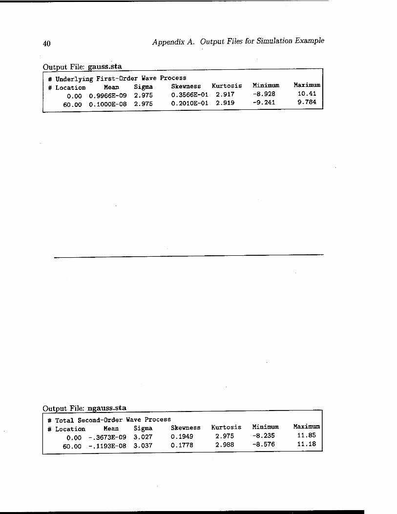
The output files created are: gauss.hist, ngauss.hist, gauss.stat, and ngauss.stat. The contents of these are listed in the following table:

Output File gauss.hist

ngauss.hist gauss.stat

ngauss.stat

Contents First-Order Time History Second-Order Time History First-Order History Statistics Second-Order History Statistics

Each of these output files is given in the Appendix A.

Figures 2.2 and 2.3 show a comparison of the simulated histories. Figure 2.2 compares the simulated first- and second-order wave time histories at the same location (the first of the two requested, defined arbitrarily as x=0 [m]). The file ngauss.stat includes the estimated skewness of the second-order waves. At this location the second-order wave history has a skewness of about 0.2. This positive skewness (compared to zero skewness of Gaussian waves) indicates the systematic nonlinear effects. This also gives rise to an asymmetry between peaks and troughs; in particular, the extreme wave crest in the second-order simulation systematically exceeds the corresponding extreme trough in absolute value. This tendency may be significant for potential deck impact problems, particularly in older jacket structures with relatively low deck levels.

Figure 2.3 compares the second-order wave histories predicted by simulation at the two spatial locations, separated by 60 [m]. The phase lag at these two locations is evident in the plot. It can be seen that a crest height at 0 [m] does not necessarily imply a crest of the same height at 60 [m].

2.5. Example 15

CO

i LU

100 Time (sec)

200

Figure 2.2: Simulated first- and second-order wave histories at location 0.0

15

10 -

c o CO

LU

-10

Location = 0.0 Location = 60.0

50 100 Time (sec)

150 200

Figure 2.3: Simulated second-order wave histories at location 0.0 and 60.0

Chapter 3

Identification of First-Order Waves

3.1 Introduction

In ocean engineering practice it is common to assume the waves to be Gaussian and any nonlinearity in the waves is embedded in the structural response analysis (e.g., WAMIT, 1995). It has been shown in Winterstein and Jha, 1995 that observed time histories generally contain nonlinearities, it is thus imperative to remove any second-order effects in the incident waves so that we do not double-count these effects in the resulting response estimation. Recent studies (Ude and Winterstein, 1996) have demonstrated the impact of double-counting such second-order effects on various structural response characteristics.

The methodology to identify the underlying first-order waves is to seek the implied first-order wave history which, when run through the second-order wave predictor, yields an incident wave that agrees with the target observed history at each time point. This identification is performed using a Newton-Raphson scheme to achieve simultaneous convergence at each complex Fourier component. If the observed history has N components, we iteratively solve N simultaneous nonlinear equations to identify the first-order components.

Due to computer memory limitations, the identification of the first-order history is performed on short contiguous windows of the observed history. This window size (mien) can be made equal to the observed history length in WAVEMAKER if the computer has sufficient RAM and swap space.

17

18 Chapter 3. Identification of First-Order Waves

3.2 Methodology

The idea here is to identify the implied first-order history 771 (<) (of an observed history Vobs(t)) which, when run through the second-order predictor, yields an incident wave that agrees with r)ohs(t). In the first-order wave process 771(f) (see Eq. 2.7), written as a Fourier sum of N frequencies,

N/2 N

mit) = E A* cosM + '*) = E x^kt ^l) k=\ k=l

we need to identify only the lower half Xk components, since the upper half values are complex conjugates of the lower half. Let us denote Xk = Uk + iVky where Uk, Vk

are the real amd imaginary parts of the complex Fourier component Xk, respectively.

The predicted second-order wave process (see Eq. 2.11) as evaluated from the

QTFs is

N/2 N/2

Am(t) = 2Re £ £ XmXnH+J^^ + XmX*nH^w—]t (3-2)

This may be rewritten in the form of a Fourier sum as

Ar72(t) = Ene^ (3-3)

where Yk = Yk+ + Yk are the combined sum and difference frequency components.

Here again, Yk possesses conjugate symmetry so that only the lower half contains unique information. Yk+ can be shown to be

y+ = £ XmXnH+n m+n,k

= £ [(UmUn-VmVn) + i(VmUn + UmVn)]H+n (3.4)

where the summation symbol indicates a double summation

N/2 N/2

J2 = £ E such that w™ + ^ = uk (3.5) m+n,k ro=l n=l

and

Yf. — 2_s ■^■m-^n^mn m—n,k

= E [(UmUn + VmVn) + i(VmUn-UmVn)]H-n (3.6) m—n,k

3.2. Methodology 19

where N/2 N/2

£ =EE SUch that \U™ ~ ^"1 m—n,k m=l n=l

Uk

The combined predicted wave process is

Vpred(t) = m(t) + &V2(t)

(3.7)

(3.8)

The identification scheme strives to simultaneously match r)pre(i(t) to the observed wave history 77obs(*) at every value of t. Alternatively, we can perform the identification in the frequency domain and strive to simultaneously match the predicted Fourier components to the observed Fourier components at all frequencies.

Vobs(t) can be represented in the frequency domain as

N

Vobs(t) = £ V"** (3.9) jfc=i

where Zks also possess conjugate symmetry. If the first-order components are identified exactly, from Eq.s 3.1, 3.3 and 3.9 we will have

Zk = Xk + Yk ; forallfc = l...iV/2 (3.10)

Note that the upper half values can be obtained from conjugate symmetry of the lower half values. In the Newton-Raphson identification scheme we will try to simultaneously minimize Xk + Yk - Zk; for k = 1... N/2 to achieve convergence. Now, this scheme requires a Jacobian of Xk + Yk - Zk with respect to the unknowns Xfc-such a complex differentiation will lead to numerical discontinuities so we will minimize an

equivalent real function yJY>i fk/N instead, where for k = 1... N/2

h = Re(Xk + Yk-Zk)

fk+N/2 - lm(Xk+Yk- Zk) (3.11)

The identification of the lower half Xk values requires a simultaneous solution of the nonlinear equations in 3.11 such that fk-*0 for all k = 1 N, or alternately J*£,i fk/N -4 0. We will formulate the Newton-Raphson scheme in vector form as

(3.12) " ReX "

ImX +

" ReY ' ImY

— ReZ ImZ

where bold face letters denote vectors, and vectors X,Y,Z contain the complex Fourier components Xk, Yk, Zk, k = 1... N/2, respectively. Here, [-§j^] is a vector containing the real part of X in the upper half and the imaginary part of X in the lower half.


Let us denote

A = " ReX "

ImX

B = " ReY "

ImY

C = ReZ ImZ

u

(3.13)

Note that the vector A, of length N, is constructed such that lower half values are the real parts of Xk; k = 1.. .N/2 and the upper half is the imaginary part of Xk\ k = 1...N/2. Similarly, B and C, each of length JV, contain real and imaginary parts of the lower half of the second-order correction and the observed Fourier components, respectively. The elements of A and B are denoted by at and bk, respectively, where l,k = 1...N. The objective function in vector notation now

is f (A) = A + B - C (3.14)

A first-order Taylor approximation of f(A) about a given A<°> is

f(A) = f(A<°>) + [J](A-A<°>) (3.15)

where [J] is a NxN Jacobian matrix denoting the derivatives of the elements fk in vector f (A) with respect to each of the unknowns a/ in A where k,l= 1...N. The Newton-Raphson scheme at iteration p + 1 is then formulated as

A(P+D = AW + h (3.16)

where h, a vector of length N, is found from a Cholesky decomposition followed by a back-substitution scheme from

(3.17) [ J]h = -f (AW)

It can be easily shown from Eq. 3.14 that the entries JM of the matrix [J] are

(3.18)

where dbk/dat indicates the partial derivative of bk with respect to ah and

To find dbk/dai, recall from notation in 3.13

bk = ReYk and bk+N/2 = lmYk for k = l...N/2

ai haXi = Ui and al+N/2 = ImXi = VJ for I = 1... N/2

3.2. Methodology 21

so that from Eq.s 3.4 and 3.6 we have

^ = £ {Vn6na + UMB+M+ E (.Un8ml + Um5nl)H- OUi m+n,k m—n,k

^± = £ -(Vn6ml + Vm5nl)H+n+ £ (VnSml + Vm5nl)H-n (3.20) oVi Tn-\-nJt Tfl—fljt

?^k = £ (VmSnl + Vn6mi)H+n + £ {Vm6nl-Vn5ml)H-v Out tn+n,k m—n,k

dlmYk = Y, (UnSmi + Um6ra)H+n+ £ {Un5ml - Um8nl) H;

°Vl m+n,fc

Schematically,

[J] = [I] +

where [J] is the identity matrix.

dUi

dUt

171—fl,fc

dReYk

dV,

dVt

(3.21)

3.2.1 Newton-Raphson Scheme

The algorithm for the Newton-Raphson scheme followed in WAVEMAKER is

1. Estimate C from observed history (Eq.s 3.9, 3.13) 2. Initial Guess A = C 3. Estimate B from A (Eq.s 3.4, 3.6, 3.13) 4. Find f(A) (Eq. 3.14) 5. Find [J] (Eq.s 3.20, 3.21) 6. Solve [J]h = -f(A) to find h 7. Update A = A + h 8. Check Convergence (see next section):

If converged terminate else go to 3

3.2.2 Convergence Criteria

The Newton-Raphson iteration scheme is terminated based on the following condi-

tions:


• Program Converged: If the rms of the increment vector h = y £f h\/N is less than a specified tolerance, the program is said to have converged. This convergence tolerance is specified as a fraction a (= 0.0001 in WAVEMAKER) of the standard deviation of the observed wave history av,obs-

• Program Diverging: If the rms of the identified first-order history a^i at any iteration p is larger than a specified fraction ß (= 200 in WAVEMAKER) of CT^obs then the identification scheme is restarted with a smaller initial guess which is a truncated and scaled down version of C. The truncation point is at twice the peak spectral frequency of r)obs(t) and the scaling factor is factnur (= 0.9r in WAVEMAKER), where r is the number of restarts heeded so far. Thus the restart guess in complex Fourier notation is

v _ / fo-ctnurZk ; Uk < 2u;peak /g 22) k ~ I 0 ; otherwise V ' ;

Maximum Iterations Reached: If the maximum allowed iterations, specified by the variable mxiter (= 10 in WAVEMAKER), is reached and the program has still not converged, then the program restarts the Newton- Raphson identification scheme with a smaller initial guess = factnurC. Maximum Restarts Reached: If the maximum allowed restarts, specified by the variable nuiter (= 5 in WAVEMAKER), is reached then the program terminates the identification scheme in the present window and proceeds to identify in the next observed history window.

3.2.3 Implementation

The first-order components for the observed wave history, of length 7Vobs, are identified in contiguous windows, each of length N < Nobs. The identification analysis is performed in this way to minimize the computer memory usage by WAVEMAKER. Recall that the Jacobian matrix [J] is a NxN matrix and the memory usage is directly governed by the matrix size of this variable. In principle, if there is sufficient memory we could set N = iVobs and identify the first-order component for the entire observed history in one window, however, this is not usually not the case and we resort to identifying in contiguous windows, as shown in Fig. 3.1.

The first-order component is identified independently in each of the windows in sequence. The last window is skipped if its contains points less than N.

3.3. Input Specification 23

512 1024 1536 2048 2560 3072 3584 4096 Time Index

Figure 3.1: Identification of first-order wave components is done in contiguous windows of the observed history

3.3 Input Specification

The input specification for the identification of first-order wave process is in a command- line format similar to the simulation input. A typical input file for identification is:

# Typical input file: syntax description

identify filename dt winsize depth value define varlimit value define gravity value write history filenamel filename^

# Typical input file: syntax description Any line beginning with a "#" symbol is treated as a comment line and is ignored.


Blank lines in the input file are ignored, as well.

define varlimit value define gravity value The keywords varlimit, gravity have the same meaning as in the simulation section and the user is referred to this section to understand the usage of these commands.

depth value The keyword depth as in the simulation section indicates the water depth at which the identification analysis is to be performed.

identify filename dt winsize The keyword identify indicates to the program that the user intends to identify the underlying first-order wave history for a given observed wave history. This command requires three arguments which in sequence are:

• filename: The name of the file, a character string, containing the observed wave time history for which the underlying first-order wave history is to be identified. The data in the first column in filename is read as the observed wave time history. Any blank lines in filename or lines that do not begin with a number are ignored.

• dt: This value, a real number, indicates the time resolution of the wave history provided in filename. In other words, dt is the time difference between two successive elevation values in the observed wave history.

• urinsize: An integer value indicating the window size or the number of points of the provided wave history to be used in each Newton-Raphson iteration. The first-order wave components are identified in windows (of size winsize) in sequence for the provided time history. If the last window contains number of points less than winsize then this window is ignored and the first-order components are not identified in this window.

The maximum value of winsize is mien set to 512 points in WAVEMAKER and can be changed according to the user's needs or according to the computer's limitations. Note that we require mien < 2xmxgrd in the program. These dimension values are set in this way so as to minimize the memory requirements of WAVEMAKER.

write history filenamel filename2 The command write history is used to specify the file names where the identified histories are to be written. The identified first-order wave history is written in file filenamel and the identified second-order, combined first- and second-order, and the observed wave histories are written in file filename^. Default values assigned to filenamel and filename2 are gauss.hist and ngauss.hist, respectively.

3.4. Output Format 25

3.4 Output Format

The output file names are governed by the command write history filenamel filename2 with default names being gauss.hist and ngauss.hist for filenamel and filename2,

respectively.

filenamel contains the identified first-order wave history in a column of real numbers. Each line of this file contains one real number indicating the elevation of the first-order wave history (see example output files in Appendix B). The time resolution of this first-order history is dt, equal to the dt provided in the input file using the command identify. This file also contains comment lines that begin with a "#" symbol as the first character on the line. The first comment line contains information on the contents of the file, and the following comment lines contain 3 integers: the first is the window number being identified, the second is the number of iterations required for convergence, and the third is the number of restarts needed for convergence.

filename2 contains the second-order correction, the combined first- and second- order waves, and the observed wave time history. The second-order correction is found from the identified first-order waves, and these two are added together to yield the combined second-order wave history. These histories are provided in three columns in filename2, or in other words each line contains three real numbers: the first is the second-order wave elevation, the second is the combined identified wave elevation, and the third is the observed wave history (see example output file in Appendix B). A match of the total identified and the observed wave histories will verify successfuly identification by WAVEMAKER. The time resolution of each of these histories is dt. This file also contains comment lines beginning with a "#" symbol that provides information similar to the comment lines in filenamel.

3.5 Examples

In this section we present two sample problems to illustrate the use of the identification capabilities of WAVEMAKER. Example 1 is based on the example presented in the simulation chapter. Sample input and output files of this identification example are included in the distribution diskette. Example 2 presented here demonstrates the identification of first-order components of a measured wave tank history. Note that sample input or output files of this second example are not included in the distribution.


3.5.1 Example 1

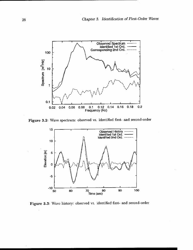
The example of the simulation capabilities of WAVEMAKER involved simulating a second- order wave history characterized by a JONSWAP spectrum with Hs = 12 [m], Tp = 14s and 7 = 3.3 in 70 [m] water depth. We will use the combined second-order simulated history and try to identify its first-order wave component and compare it to the input first-order component used to simulate the combined wave history. The input file for the identification run is

# Wave Identification Input File

identify hist.dat 0.5 512 depth 70.0 write history gauss.ide ngauss.ide define varlimit 0.01 define gravity 9.807

Alternatively, if we intend to use the default definitions in the program then our input file could be (this will produce the same output as the extended version of the input file):

# Wave Identification Input File # (Alternative format)

identify hist.dat 0.5 512 depth 70.0 write history gauss.ide ngauss.ide

The input file hist.dat contains a column of real numbers (see sample files listed in the appendix) which will be read in as the observed wave history. The first- order components will be identified for this observed history and placed in the file gauss.ide. The corresponding second-order components, the combined identified history and the observed wave history are written in the file ngauss.ide.

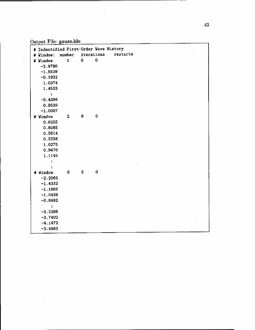
Output File gauss.ide

ngauss.ide

Contents Identified First-Order Time History Corresponding Second-Order Time History

3.5. Examples 27

Figure 3.2 shows the observed wave spectrum and the identified first-order spectrum along with the corresponding second-order wave spectrum. We see that small second-order contribution to the power spectrum, roughly a decade below the first- order spectrum even at frequencies twice the peak spectral frequency, suggests the difficulty in identifying these components. Figure 3.3 shows the observed wave history and the identified first-order wave history in cycles around the maximum crest height. Compare this to the simulation example where we solve the forward problem of finding the combined (first- plus second-order) history from a given underlying first-order wave spectrum. The identified first-order component in Fig. 3.3 is almost the same as the underlying first-order component (denoted Gaussian) in Fig. 2.2 and these two are shown together in Fig. 3.4. Note how close the two first-order components are, and any numerical differences can probably be further reduced by using a larger window size (greater than 512, for example) in the identification scheme.

3.5.2 Example 2

In this example we will identify the underlying first-order wave component for a measured wave tank history that reflects a water depth of about 300m. For this example the measured history is located in file wave.dat and has a dt = 0.424264 seconds. We will use windows of winsize = 512 to identify the first-order components. The input to WAVEMAKER is:

# Wave Identification Input File # using default definitions

identify wave.dat 0.424264 512 depth 300.0

Figure 3.5 shows a portion where the maximum crest height occurs in the measured wave tank history. The figure also shows the identified first-order and the corresponding second-order wave histories. Note how the second-order wave component affects the first-order peaks, amplifying the crests and moderating the troughs. Figure 3.6 shows the wave spectra for the measured history along with the first-order and the second-order spectra. Again, observe that the second-order energy is significantly small compared to the first-order, however, phase locking of the first- and the second- component (Fig. 3.5) leads to larger crests and flatter troughs.


r 1 1 1 1 1 1— i A Observed Spectrum

x—y laeniiTiea IST ura. \ oorresponaing ^na vjra. — ■ —

100 \ .«£%&

"N" V » I \ A

\ yCx /*

£ 10 -

E \ 'O-- 3 V v^\ h-

8 it

D. CO i

'^'- / /

/■- A /

\ A J i \ i V/ - \ i\! \y

■V" V

0.1 W' > ■ 1 1 1 1 1 :

0.02 0.04 0.06 0.08 0.1 0.12 0.14 0.16 0.18 0.2 Frequency (Hz)

Figure 3.2: Wave spectrum: observed vs. identified first- and second-order

15

c o eo

UJ

-10

Observed History Identified 1st Ord.

Identified 2nd Ord.

50 60 70 80 Time (sec)

90 100

Figure 3.3: Wave history: observed vs. identified first- and second-order

3.5. Examples 29

15

10

-10

Input IstOrd. Identified 1st Ord. +

50 100 Time (sec)

150 200

Figure 3.4: Identified first-order vs. actual first-order wave history


20

-15

-i r-

First-order Second-order

Observed

_l L-

3960 3980 4000 4020 4040 4060 4080 4100 4120 Time Index

Figure 3.5: Wave history in wave tank: observed vs. identified first- and second-order

0.1

First-order Second-order

Observed

0.05 0.1 0.15 Frequency (Hz)

0.2 0.25

Figure 3.6: Wave spectrum in wave tank: observed vs. identified first- and second-order

Chapter 4

Distribution

The WAVEMAKER routine and example files have been distributed on a DOS formatted 3.5 inch floppy diskette. The diskette contains the source code files (of the form *.f), example input (*.inp), and output files (*.sta, *.his, and *.ide). The diskette also contains this manual in postscript format in manual.ps.

4.1 Copying the Diskette

Copy the contents of the diskette on to your host computer (computer on which you will run WAVEMAKER). After the copying is done, your host computer should have:

• Example input files wavmkr.inp, wavide.inp, and hist.dat. • Example output files gauss.his, ngauss.his, gauss.sta, ngauss.sta,

gauss.ide, and ngauss.ide. • manual.ps containing this manual in postscript format • all the source files * .f and Makefile

Table 4.1 shows the input and output files that are specific to the simulation and to the identification examples.

31

32 Chapter 4. Distribution

Table 4.1: Distributed Files for Simulation and Identification Examples Simulation Example

File Type Input File

Output Files

File Type Input Files

Output Files

File Name wavmkr.inp gauss.his

ngauss.his

gauss . sta

ngauss .sta

Description Input to WAVEMAKER Simulated first-order wave histories at each specified location Simulated combined first- and second-order wave histories at each specified location Statistics of the simulated first- order histories at each specified lo cation Statistics of the simulated combined histories at each specified location

Identification Example File Name wavide.inp hist.dat

gauss.ide ngauss.ide

Description Input to WAVEMAKER Observed wave history for which underlying first-order history is to be identified Identified first-order wave history Identified second-order, combined first- and second-order, and observed wave histories

4.2 Compiling the Source

On a Unix workstation, the Makefile can be used to build the WAVEMAKER executable. To compile on your host Computer:

• change directory to the subdirectory containing the source code files • type "make wavmkr" (without the double quotes) at the Unix prompt

and press return

The above will compile all the files listed in Makefile and link them to make the executable wavmkr. Note that the executable wavmkr is still in the current directory, and may be moved to the directory which contains the input file, or you can specify the path to the executable file in order to run it from other directories.

4.3. Executing the Routine 33

On other operating systems and architectures, follow whatever is the standard procedure for compiling and linking FORTRAN source code distributed over multiple files.

WAVEMAKER has been developed on a Sun Sparcstation2, using version 1.4 of the Sun FORTRAN compiler. Every attempt has been made to adhere to the ANSI FORTRAN 77 standard, ensuring portability of the code.

4.3 Executing the Routine

At the Unix prompt type "wavmkr < wavmkr.inp" (without the double quotes) in order to execute WAVEMAKER and perform the simulation example analysis. The program reads input from the standard logical input unit. The logical units for standard input, standard output, and standard error are all used in WAVEMAKER. On the Sun compiler, 0 is used for standard error, 5 is standard input and 6 is standard output. If the appropriate unit numbers are different, they can be set using the IOER, IOIN, and IOOU variables in the WAVEMAKER driver program, and the package can be recompiled.

Run the example problem using the complied code to check if you get the same output as provided in the example output files. Note that wavmkr will overwrite any existing file if you specify its name as the target output file using the write command in the input file.

Similarly, at the Unix prompt type "wavmkr < wavide.inp" (without the double quotes) in order to execute WAVEMAKER and perform the identification example analysis. The resulting output histories can be compared to the corresponding example output histories to verify successful compilation of WAVEMAKER.

34 Chapter 4. Distribution

List of References

Bitner-Gregerson, E., and Haver, S. 1991. Joint environmental model for reliability calculations. Pages 472-478 of: Proceedings of the 1st international offshore and polar engineering conference (ISOPE).

Borgman, L. E. 1969. Ocean wave simulation for engineering design. Journal of waterways, harbors division, 95(4), 556-583. ASCE.

Jha, A. K., and Winterstein, S. R. 1995. Second-order random waves: Simulation in time and space. Tech. rept. RMS-17. Reliability of Marine Structures Program, Stanford University, Dept. of Civil Engineering.

Langley, R. S. 1987. A statistical analysis of non-linear random waves. Ocean engineering (pergamon), 14(5), 389-407.

Longuet-Higgins, M. S. 1963. The effect of non-linearities on statistical distributions in the theory of sea waves. Journal of fluid mechanics, 17(3), 459-480.

Marthinsen, T., and Winterstein, S. R. 1992. On the skewness of random surface waves. Pages 472-478 of: Proceedings of the 2nd international offshore and polar engineering conference, san francisco. ISOPE.

Molin, B, and Chen, X. B. 1990. Calculation of second-order sum-frequency loads on tip hulls. Tech. rept. Institute Francais du Petrele Report.

SWIM, 2.1. 1995. SWIM: Slow wave-induced motions- user's manual. Dept. of Ocean Engineering, M.I.T.

Ude, T. C. 1994. Second-order load and response models for floating structures: Probabilistics analysis and system identification. Tech. rept. RMS-16. Reliability of Marine Structures, Dept. of Civil Engr., Stanford University.

Ude, T. C, and Winterstein, S. R. 1996. Calibration of models for slow drift motions using statistical moments of observed data. In: 6th international offshore and polar engineering conference ISOPE. to appear.

35

og List of References

Vinje, T., and Haver, S. 1994. On the non-Gaussian structure of ocean waves. Pages 453-480 of: Proceedings of the 7th international conference on the behaviour of offshore structures (BOSS), vol. 2.

WAMIT, 4.0. 1995. WAMIT: A radiation-diffraction panel program for wave-body interactions-user's manual. Dept. of Ocean Engineering, M.I.T.

Winterstein, S. R., and Jha, A. K. 1995. Random models of second-order waves and local wave statistics. Pages 1171-1174 of: Proceedings of the 10th engineering mechanics speciality conference. ASCE.

Appendix A

Output Files for Simulation Example

37

38 Appendix A. Output Files for Simulation Example

Output File: gauss.his

# Underlying First-Order Wave Process # #

Wave Elevation at Spatial Location

Time(sec.)

0.000000

0.500000

1.000000

1.500000

2.000000

2.500000

3.000000

3.500000

4.000000

4.500000

5.000000

5.500000

6.000000

6.500000

7.000000 7.500000

8.000000

8.500000

9.000000 9.500000

10.000000

10.500000

11.000000

11.500000

2046.500000 2047.000000

2047.500000

0.00 -3.189 -1.754 -0.239 0.906 1.436 1. 1. 1. 1, 2. 2,

.681

.623

.595

.862

.282

.802 3.230 3.263 2.448 1.403 0.553

-0.121 -0.773 -1.216 -1.588 -2.433 -3.543 -4.310 -4.343

-3.871 -4.266 -4.040

60.00 -4.754 -5.466 -5.410 -4.667 -3.660 -2.714 -1.676 -0.875 -0.137 0.582 1.211 1.379 1.263 1.252 1.572 2.166 2.447 3.076 3.472 3.272 2.507 1.492 0.022

-1.441

0.056 -1.729 -3.447

Note that ":" indicates more numbers. Since the files are long, we present truncated versions of the output files.

39

Output File: ngauss.his Total Second-Order Wave Process

Wave Elevation at Spatial Location

Time(sec.)

0.000000

0.500000

1.000000

1.500000

2.000000

2.500000

3.000000

3.500000 4.000000

4.500000

5.000000

5.500000 6.000000

6.500000

7.000000

7.500000

8.000000

8.500000

9.00000.0

9.500000

10.000000

10.500000

11.000000

11.500000

12.000000

12.500000 13.000000

13.500000

2046.500000

2047.000000

2047.500000

0.00 -3.487 -2.747 -0.970 0.975 1.927 1.920 2.210 1.738 2.034 2.353 2.974 3.595 3.481 1.913 1.236 0.644 0.019

-0.826 -0.572 -1.304 -2.734 -3.700 -3.854 -4.087 -3.686 -2.784 -1.532 -1.026

60.00 -4.814 -5.039 -4.773 -4.589 -3.459 -2.768 -1.844 -0.534 -0.256 0.534 1.072 2.033 1.523 1.684 1.334 2.374 2.724 3.160 3.945 3.330 2.573 1.296

-1.195 -1.811 -2.346 -2.356 -2.498 -2.256

-3.594 -1.165 -3.918 -3.159 -3.660 -4.297

40 Appendix A. Output Files for Simulation Example

Output File: gauss.sta .

# Underlying First-Order Wave Process # Location Mean Sigma Skewness Kurtosis Minimum Maximum

0.00 0.9966E-09 2.975 0.3566E-01 2.917 -8.928 10.41 60.00 0.1000E-08 2.975 0.2010E-01 2.919 -9.241 9.784

Output File: ngauss.sta

# Total Second-Order Wave Process # Location Mean Sigma Skewness Kurtosis Minimum Maximum

0.00 -.3673E-09 3.027 0.1949 2.975 -8.235 11.85 60.00 -.1193E-08 3.037 0.1778 2.988 -8.576 11.18

Appendix B

Input/Output Files for Identification Example

41

42 Appendix B. Input/Output Files for Identification Example

Input File: hist.dat .

-3.487 -2.747 -0.970 0.975 1.927 1.920 2.210 1.738 2.034 2.353 2.974 3.595 3.480 1.914 1.236 0.644 0.019

-0.826 -0.572 -1.304 -2.734 -3.700

-1.458 -2.043 -2.767 -3.241 -3.594 -3.918 -3.660

Note that ":" indicates more numbers. Since the files are long, we present truncated versions of the output files.

43

Output File: gauss.ide # Indentified First-Order Wave History # Window: number iterations restarts # Window 16 0

-2.9780 -1.5528 -0.1932 1.0374 1.4503

-0.4398 0.9539 -1.0007

# Window 2 8 0 0.6255 0.8085 0.5614 0.5256 1.0275 0.9476 1.1145

# Window -2.2065 -1.4332 -1.1666 -1.0438 -0.8492

-3.2288 -3.7402 -4.1472 -3.4963

44 Appendix B. Input/Output Files for Identification Example

Output File: ngauss.ide # Identified 2nd-0rder Wave, Identified Total Wave, Input Wave History # Window: number iterations restarts

Window -0.5090 -1.1942 -0.7768 -0.0624 0.4767

-0.0489 -0.8702 -0.3039 2.0597

Window 0.1029 0.4542 0.3126 0.0864 0.1123 0.4375 0.0240

# Window -0.3825 0.3802 0.3296 0.2628 0.1202

-0.0122 0.1462 0.2292 -0.1637

1 6 -3.4870 -2.7470 -0.9700 0.9750 1.9270

7070 3100 6500 0590

8 .7284 .2627 .8740

0.6120 1.1399 1.3851 1.1385

8 5 -2.5890 -1.0530 -0.8370 -0.7810 -0.7290

-3.2410 -3.5940 -3.9180 -3.6600

0 -3.4870 -2.7470 -0.9700 0.9750 1.9270

-1.7070 -1.3100 0.6500 1.0590

0 0.7320 1.2660 0.8710 0.6120 1.1390 1.3860 1.1380

0 -2.5890 -1.0530 -0.8370 -0.7810 -0.7290

-3.2410 -3.5940 -3.9180 -3.6600

Appendix C

Random Models of Second-Order Waves and Local Wave Statistics

The following paper demonstrates the application of these nonlinear wave models and simulation techniques. It also shows how wave moments can be estimated analytically, and resulting estimates of extreme waves formed. Finally, various local wave characteristics found from the simulation are compared with field and wave tank data.

It has appeared in the Proceedings of the 10th Engineering Mechanics Specialty Conference, ASCE, held in Boulder, May 1995.

45

From Proceedings, It)"1 ASCE Eng. Mech. Specialty Conference Boulder, Colorado, Vol. 2, 1995, pp. 1171-1174

RANDOM MODELS OF SECOND-ORDER WAVES AND LOCAL WAVE STATISTICS

Steven R. Winterstein and Alok K. Jha Civil Eng. Dept., Stanford University

Abstract

We consider second-order random models of ocean waves at arbitrary water depths. We derive convenient new analytical results for wave moments, and show results for crests and other local wave statistics. Theoretical predictions are compared with observed wave tank results in extreme seas.

Introduction

Nonlinear hydrodynamic effects are of growing interest for ocean structures and vessels. This has spurred development of efficient methods to estimate statistics of second-order hydrodynamic models (e.g., Winterstein et al, 1994). Here we apply these to one of the most fundamental nonlinearities in ocean engineering: the wave elevation T}(t) at a fixed spatial location.

Linear wave theory results in a Gaussian model of 77(f). This ignores the marked asymmetry of 77(f): wave crests that systematically exceed subsequent troughs. This has several practical implications: (1) asymmetric waves are more likely to strike decks of offshore platforms, particularly older Gulf-of-Mexico structures with fairly low decks; and (2) unusually large dynamic response has been found in high, steep waves that may not follow linear theory.

Second-order random wave models are not new; indeed, they have been a research topic for more than 30 years (e.g., Longuet-Higgins, 1963) and remain so today (e.g., Marthinsen and Winterstein, 1992; Hu and Zhao, 1993; Vinje and Haver, 1994). How- ever, they have not yet entered common offshore engineering practice, which applies either (1) random linear (Gaussian) waves or (2) regular Stokes waves that fail to pre- serve Sn(Lj), the wave power spectrum. Several drawbacks to second-order random waves may be suggested: (1) they omit potentially important higher-order effects; and (2) convenient statistical analysis methods for second-order models are often lacking. We seek to address both concerns here—the first through systematic comparison of theory with observed wave tank results in extreme seas. The second issue is met by fitting new analytical results for wave moments, and using these to construct simple Hermite models of extreme crests.

Statistics of Second-Order Models

Our "input" is the first-order, Gaussian wave process 771(f) from linear theory. The standard Fourier sum for rji(t) is then ReJ2Ckexp(ioJkt), in which Cfc=Afcexp(i^) in

1171

SECOND-ORDER WAVES 1172

terms of Rayleigh distributed amplitudes, Ak, and uniformly distributed phases <f>k. The resulting "output" is x(t)=xi(t) + x2(t), in which

X! = Re £ CkEte***; *2 = Re £ £ CtC,[^^»( + H^^*] (1) fc * j

Here the transfer function #* describes first-order effects, while H& and il^ reflect second-order effects at sums and differences of all wave frequencies (w* ± o>/). In our case a?(<) is the second-order wave itself, for which fi^i and -^W are 6iven analytically (e.g., Marthinsen and Winterstein, 1992), and Hk=l. The same analysis applies more generally to the diffracted wave, applied force and response of large-volume structures, with numerical Hk and Hui estimates from second-order diffraction (Winterstein et al,

1994). Because x(t) is non-Gaussian, interest focuses on its skewness a3 and kurtosis a4.

In terms of the significant wave height Hs=4<rm and peak spectral period TP, these

are a3o* = m31(TP)H4

s + m33(TP)H6s (2)

(a4 - 3)4 = m42(TP)H§ + m44{TP)Hl (3)

The mij(Tp) are "response moment influence coefficients," the contribution to response moment (cumulant) i due to terms of order 0(x3

2). In general these are conveniently calculated from Kac-Siegert analysis (Eqs. 12-15, Winterstein et al, 1994). We assume here the spectrum of 771(f) is of the form H2

sTPf(uTP), so that r?x(i) scales in amplitude with Hs and in time with TP.

It is useful to define the unitless wave steepness sP=Hs/LP, in which the charac- teristic wave length LP=gTp/2ir uses the linear dispersion relation. For deep-water waves the coefficients mij(TP) are proportional to Lp3. Retaining leading terms in sP

from Eqs. 2-3: «3 = k3sP ; a4 - 3 = &4<*3 (4)

In particular, for a JONSWAP wave spectrum with peakedness factor 7, we have fit the following &3 and k4 expressions to results for a wide range of depths:

k3 = %. = 5.457-084 + •135(^-)-1"22 ; ** = ^ = l.^-*20 (5) sP -Lp a

3

The second term in this result for a3 reflects the effect of a finite water depth d: in shallower water a3 grows, as the waves begin to "feel" the bottom.

Note also that while the skewness varies linearly with steepness, the kurtosis varies quadratically. This suggests that nonlinear effects will be most strongly displayed by the skewness, and hence by the wave crests rather than the total peak-to-trough wave height. This second-order model may less accurately predict kurtosis, however, as higher-order omitted effects may be of the same order of magnitude.

Numerical Results

Figure 1 compares skewness predictions with results from wave tank tests. The tests include 18 large seastates (target #s=14.5m-15.5m), each over 3 hours in length, at water depths exceeding 300m. Figure 1 shows the resulting skewness and steepness in each hour of each test. While there is considerable scatter, regression on these data


gives the estimated slope &3=5.50, remarkably close to Eq. 5 with 7=1. The scatter in Figure 1 is also consistent: the observed aaz is found well-predicted by simulated hourly segments of second-order seastates. Figure 2 shows kurtosis estimates to deviate, however. The data yield the estimate fc4=4.2, roughly 3 times the value in Eq. 5 regardless of 7. This again supports theory, which suggests that unlike the skewness, the kurtosis may be notably affected by unmodelled, higher-order effects.

Wave Crests. Figure 3 shows the observed distribution of crest heights. These results combine six seastates with the same target spectrum, and hence give roughly 20 hours of similar wave conditions. As expected the Rayleigh model, based on linear theory, is significantly unconservative. An alternative empirical model (Haring et al, 1976) offers an improvement, but only mildly changes the Rayleigh for these deep-water conditions. Better agreement is found from a Non-Gaussian (Hermite) model, which uses a cubic distortion of the normal process (and hence its Rayleigh peaks) to match a3 and a4 (Winterstein et al, 1994). Here estimates of a3 and a4 use Eq. 5, tripling its k4 value to reflect unmodelled effects. These give excellent agreement with observed moments, though still somewhat unconservative crest predictions at higher levels.

Local Wave Characteristics. Figure 4 shows the conditional mean and standard deviation of crest height, given the peak-to-trough wave height. Again the data use 20 hours of wave tank studies, all with the same target wave spectrum. Also shown are corresponding estimates from simulation of Gaussian and Non-Gaussian (second-order) models. Due to the symmetry of the Gaussian model, its crests are on average 50% of the total wave height. The data shows systematically larger crests. The second-order model is found to predict this vertical asymmetry quite accurately.

We may also consider horizontal wave asymmetry: do crest front periods—during which 77 increases from its mean level to a crest—differ statistically from subsequent crest back periods? This temporal asymmetry is not predicted by either the Gaussian or second-order model. It is difficult, however, to find this asymmetry in the data: Figure 5 shows observed crest fronts to be quite close to 50% of the total crest period. Finally, Figure 6 shows the variation of wave period with crest height. All results show the same trend of increasing periods over small-to-moderate heights, and roughly constant period at large heights. The Non-Gaussian model appears to somewhat better predict results at larger crest height levels.

References Haring, R.E., A.R. Osborne, and L.-P. Spencer (1976). Extreme wave parameters based

on continental shelf storm wave records. Proc., 15th Coastal Eng. Conf., ASCE, 151-170.

Hu, S.J. and D. Zhao (1993). Non-Gaussian properties of second-order random waves. J. Engrg. Mech., ASCE, 119(2), 344-364.

Longuet-Higgins, M.S. (1963). The effect of non-linearities on statistical distributions in the theory of sea waves. J. Fluid Mech., 17(3), 459-480.

Marthinsen, T.M. and S.R. Winterstein (1992). On the skewness of random surface waves. Proc., 2nd Intl. Offshore Polar Eng. Conf., ISOPE, 472-478.

Vinje, T. and S. Haver (1994). On the non-Gaussian structure of ocean waves. Proc., BOSS-94, 2, 453-480.

Winterstein, S.R., T.C. Ude and T. Marthinsen (1994). Volterra models of ocean structures: extreme and fatigue reliability. J. Engrg. Mech., ASCE, 120(6), 1369-1385.


CO CO <D C

i CO

TJcSüriyl vedti

data 'o Observed trend —

Predicted; gamma=1 Predicted; gamma=3

o o °

1 ' ' Hourly data" o ' Observed trend

Predicted; gamma=1

0.026 0.03 0.034 0.038 Average steepness, sp=Hs/Lp

Figure 1: Skewness: Theory vs Data

1

0.1

0.02 0.04 0.06 0.08 Squared skewness, a3A2

Figure 2: Kurtosis: Theory vs Data

15-

Q 0 0.01 r

0.001

0.0001

i+f^j—i—i—r —i—i—r T

'■

^S

T

r Heidrun \w\ 1

Heidrun ne—i \\A> Rayleigh \\ \>v Hermrte \\ \l

f Haring et al.

■ i i ■ i

\ \ V

. 1 \ \ 1 >J

0 2 4 6 8 10 12 14 16 18 20 Crest Height (m)

Figure 3: Crest Heights: Theory vs Data

ü CD <n_

■o o CD Q.

c o

1C

8

6

-Data* i

- Gaussiain o

■Ndn-r-Gäussiän

CO CD

Ö

4 6 8 10 12 Crest Period (sec)

Figure 5: Variation of Crest Front Period with Total Crest Period

10 15 20 Wave Height (m)

Figure 4: Variation of Crest Height with Wave Height

2Q ■ ■

o 8.1! o

Q?1< CD > CO

s , -Data*

Gaussian o

•Non-Gaussian +

0 5 10 Crest Height (m)

Figure 6: Variation of Crest Height with Wave Period

15

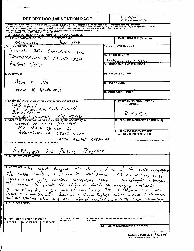
REPORT DOCUMENTATION PAGE Form Approved OMB No. 0704-0188

Public reporting burden for this collection of information is estimated to average 1 hour per response, including the time for reviewing instructions, searching data sources, gathering and maintaining the data needed, and completing and reviewing the collection of information. Send comments regarding this burden estimate or any other aspect of this collection of information, including suggestions for reducing this burden to Washington Headquarters Service, Directorate for Information Operations and Reports, 1215 Jefferson Davis Highway, Suite 1204, Arlington, VA 22202-4302, and to the Office of Management and Budget, Paperwork Reduction Project (0704-0188) Washington, DC 20503. PLEASE DO NOT RETURN YOUR FORM TO THE ABOVE ADDRESS.

1. REPORT DATE (DD-MM-YYYY)

O0-aL~/tt(, 2. REPORT DATE

^W ml* 3. DATES COVERED (From - To)

4. TITLE AND SUBTITLE

ftAMotf U/Al/ES.

5a. CONTRACT NUMBER

5b. GRANT NUMBER

hJ Poo/U-MW-O^/ 5c. PROGRAM ELEMENT NUMBER

6. AUTHOR(S) 5d. PROJECT NUMBER

5e. TASK NUMBER

5f. WORK UNIT NUMBER

7. PERFORMING ORGANIZATION NAME(S) AND ADDRESS(ES)

W 6ßoup , A r // 8. PERFORMING ORGANIZATION

REPORT NUMBER

/ZLMS-ZI

9. SPONSORING/MONITORING AGENCY NAME(S) AND ADDRESS(ES) Office of AMi/,4L ResEAtCtf

?0o tJozry Qu,ucv ST

10. SPONSOR/MONITOR'S ACRONYM(S)

11. SPONSORING/MONITORING AGENCY REPORT NUMBER

A-rrtJ: QosfJM RAtsouHJ 12. DISTRIBUTION AVAILABILITY STATEMENT

h PPfio i/eP fofc Pu U /c 7K El tASE 13. SUPPLEMENTARY NOTES

4. ABSTRACT -ffo TLfatf J«t**e^ fhl jhtory &»J »M oj Ht fa^At UA^M(k

Tht rou+fo S/«*Ja*t} & f-'^if- orJer u/«ua process w.'H A* a^l^ . ~"-

Pto»fcs. htfbry fn,^ *- /;W>* aki*-rjej -t,s^l fi,s^ry. 7"£ 1 h+tll%K+S«* 'J K* ,VHAV^

Z. CIID ICPTTCDMC 15. SUBJECT TERMS

16. SECURITY CLASSIFICATION OF: a. REPORT b. ABSTRACT c. THIS PAGE

17. LIMITATION OF ABSTRACT

18. NUMBER OF PAGES

19a. NAME OF RESPONSIBLE PERSON

19b. TELEPONE NUMBER {Include area code)

Standard Form 298 (Rev. 8-98) Prescribed byANSI-Std 239-18

wavemaker 2.0: simulation and identification of …

Documents