waves and oscillations: a prelude to quantum...
TRANSCRIPT


Waves and Oscillations

This page intentionally left blank

Waves and Oscillations
A Prelude to Quantum Mechanics
Walter Fox Smith
32010

3Oxford University Press, Inc., publishes works that furtherOxford University’s objective of excellencein research, scholarship, and education.
Oxford New YorkAuckland Cape Town Dar es Salaam Hong Kong KarachiKuala Lumpur Madrid Melbourne Mexico City NairobiNew Delhi Shanghai Taipei Toronto
With offices inArgentina Austria Brazil Chile Czech Republic France GreeceGuatemala Hungary Italy Japan Poland Portugal SingaporeSouth Korea Switzerland Thailand Turkey Ukraine Vietnam
Copyright © 2010 by Oxford University Press
Published by Oxford University Press, Inc.198 Madison Avenue, New York, New York 10016www.oup.com
Oxford is a registered trademark of Oxford University Press
All rights reserved. No part of this publication may be reproduced,stored in a retrieval system, or transmitted, in any form or by any means,electronic, mechanical, photocopying, recording, or otherwise,without the prior permission of Oxford University Press.
Library of Congress Cataloging-in-Publication DataSmith, Walter Fox.Waves and oscillations : a prelude to quantum mechanics /Walter Fox Smith.p. cm.Includes index.ISBN 978-0-19-539349-11. Wave equation. 2. Mathematical physics. I. Title.QC174.26.W28S55 2010530.12’4–dc22 2009028586
9 8 7 6 5 4 3 2 1
Printed in the United States of Americaon acid-free paper

This book is dedicated to my mother, Barbara Leavell Smith,and to my wife, Marian McKenzie

This page intentionally left blank

Preface
To the student
I wrote this book because I was frustrated by the other textbooks on this subject.Waves and oscillations are enormously important for current research, yet other booksdon’t stress these connections. The ideas and techniques that you will learn from thisbook are exactly what you need to be ready for a study of quantum mechanics. Everyphysics professor understands this linkage, and yet other books fail to emphasize it,and often use notations which are different from those used in quantum mechanics.Other books make little effort to keep you engaged. I can’t teach you by myself, norcan your professor; you have to learn, and to do this you must be active. In this book,I’ve provided tools so that you can assess your learning as you go; these are describedimmediately after the table of contents. Use them. Read with paper and pencil handy.As a scientist, you know that only by understanding the assumptions made and thedetails of the derivations can you have your own logical sense of how it all fits togetherinto a self-consistent whole. Visit this book’s website. There, you will find links tocurrent physics, chemistry, biology, and engineering research that is related to thetopics in each chapter, as well as lots of other stuff, some purely fun and some purelyeducational (but most of it both). Hopefully, there will be a second edition of this bookin the future; if you have suggestions for it, please e-mail me: [email protected].
To the instructor
Please visit the website of this book. You’ll find materials in the website that will makeyour life easier, including full solutions and important additional support materialsfor the end-of-chapter problems, lecture notes which complement the text (includingadditional conceptual questions, worked examples, applications to current researchand everyday life, animations, and figures), as well as custom-developed interactiveapplets, video and audio recordings, and much more. The following sections can beomitted without affecting comprehension of later material: 1.10, 1.12, 2.3–2.6, 3.5–3.6,4.5, 4.7–4.8, 6.6–6.7, 8.6–8.7, 9.9, 9.11, 10.8–10.9, and Appendix A. If necessary, onecan skip all of chapter 6, except for the part of section 6.5 starting with the “Coreexample” through the end of the section; however omitting the rest of chapter 6 means

viii Preface
that the students won’t be exposed to any matrix math or to the idea of an eigenvalueequation. (They are exposed copiously to eigenvectors and eigenfunctions in otherchapters, but the word “eigenvalue” is used only in chapter 6.) If you have questionsor comments, please contact me: [email protected].
Acknowledgments
This book builds on the enormous efforts of my predecessors. Like any textbook author,I have consulted many dozens of other works in developing my presentation. However,three stand out as particularly helpful: Vibrations and Waves, by A. P. French (Norton1971), The Physics of Vibrations and Waves, 6th Ed., by H. J. Pain (Wiley 2005), andThe Physics of Waves, by H. Georgi (Prentice-Hall, 1993).
I am deeply grateful to my physics colleague Peter J. Love, who cheerfullyanswered endless questions from me, taught from draft versions of the book andgave me essential feedback, and made key suggestions for several sections. I am alsomost thankful to my other colleagues in physics who supported me in this effort andanswered my many questions: Jerry P. Gollub, SuzanneAmador-Kane, Lyle D. Roelofs,and Stephon H. Alexander. I also received very valuable inputs from colleagues inmath, particularly Robert S. Manning, and chemistry, including Casey H. Londergan,Alexander Norquist, and Joshua A. Schrier. I also thank Jeff Urbach of GeorgetownUniversity and Juan R. Burciaga of Lafayette College who used draft versions of thetext in their courses, and provided helpful feedback.
I am profoundly thankful for the proof-reading efforts, and suggested edits andend-of-chapter problems from Megan E. Bedell, Martin A. Blood-Forsythe, AlexanderD. Cahill, Wesley W. Chu, Donato R. Cianci, Eleanor M. Huber, Anna M. Klales, AnnaK. Pancoast, Daphne H. Paparis,Annie K. Preston, and Katherine L. VanAken. Specialthanks are due to Andrew P. Sturner for his tireless efforts and suggestions, right up tothe last minute.
Finally, I am most deeply grateful to my family, for their support and encourage-ment throughout the writing of this book. My children Grace, Charlie, and Tom checkedup on my progress every day, and suggested things in everyday life connected towaves and oscillations. My good friend Michael K. McCutchan gave deep proofreadingand editing help, and support of all kinds throughout. Finally, words cannot expressmy gratitude for the efforts of my wife, Marian McKenzie, who did almost all thecomputerizing of figures, helped with editing, and provided the much-needed emotionalsupport. This book would never have been published without her encouragement.

Learning Tools Used in This Book
Throughout this text you will find a number of special tools which are designed to helpyou understand the material more quickly and deeply. Please spend a few moments toread about them now.
Concept test
This checks your understanding of the ideas in the preceding material.
Self-test
Similar to a concept test, but more quantitative. It will require a little work with penciland paper.
Core example
Unlike an ordinary example, these are not simply applications of the material justpresented, but rather are an integral part of the main presentation. There are some topicsthat are much easier to understand when presented in terms of a specific example, ratherthan in more abstract general terms.
Your turn
In these sections, you are asked to work through an important part of the mainpresentation. Be sure to complete this work before reading further.

x Learning Tools Used in This Book
Concept and skill inventory
At the end of each chapter, you’ll find a list of the key ideas that you should understandafter reading the chapter, and also a list of the specific skills you should be ready topractice.

Contents
Learning Tools Used in This Book ix
1. Simple Harmonic Motion 1
1. 1 Sinusoidal oscillations are everywhere 11. 2 The physics and mathematics behind simple sinusoidal motion 31. 3 Important parameters and adjustable constants of simple harmonic
motion 51. 4 Mass on a spring 81. 5 Electrical oscillators 101. 6 Review of Taylor series approximations 121. 7 Euler’s equation 131. 8 Review of complex numbers 141. 9 Complex exponential notation for oscillatory motion 161.10 The complex representation for AC circuits 181.11 Another important complex function: The quantum mechanical
wavefunction 241.12 Pure sinusoidal oscillations and uncertainty principles 26
Concept and skill inventory 29Problems 31
2. Examples of Simple Harmonic Motion 39
2.1 Requirements for harmonic oscillation 392.2 Pendulums 402.3 Elastic deformations and Young’s modulus 422.4 Shear 472.5 Torsion and torsional oscillators 492.6 Bending and Cantilevers 52
Concept and skill inventory 56Problems 58
3. Damped Oscillations 64
3.1 Damped mechanical oscillators 643.2 Damped electrical oscillators 68

xii Contents
3.3 Exponential decay of energy 693.4 The quality factor 703.5 Underdamped, overdamped, and critically damped behavior 723.6 Types of damping 74
Concept and skill inventory 76Problems 77
4. Driven Oscillations and Resonance 84
4.1 Resonance 844.2 Effects of damping 914.3 Energy flow 954.4 Linear differential equations, the superposition principle for driven
systems, and the response to multiple drive forces 994.5 Transients 1014.6 Electrical resonance 1044.7 Other examples of resonance: MRI and other spectroscopies 1074.8 Nonlinear oscillators and chaos 114
Concept and skill inventory 128Problems 129
5. Symmetric Coupled Oscillators and Hilbert Space 137
5.1 Beats: An aside? 1375.2 Two symmetric coupled oscillators: Equations of motion 1395.3 Normal modes 1425.4 Superposing normal modes 1465.5 Normal mode analysis, and normal modes as an alternate
description of reality 1495.6 Hilbert space and bra-ket notation 1535.7 The analogy between coupled oscillators and molecular energy
levels 1635.8 Nonzero initial velocities 1655.9 Damped, driven coupled oscillators 166
Concept and skill inventory 168Problems 170
6. Asymmetric Coupled Oscillators and the Eigenvalue Equation 179
6.1 Matrix math 1796.2 Equations of motion and the eigenvalue equation 1826.3 Procedure for solving the eigenvalue equation 1866.4 Systems with more than two objects 1916.5 Normal mode analysis for multi-object, asymmetrical systems 1946.6 More matrix math 1986.7 Orthogonality of normal modes, normal mode coordinates,
degeneracy, and scaling of Hilbert space for unequal masses 201

Contents xiii
Concept and skill inventory 208Problems 210
7. String Theory 216
7.1 The beaded string 2167.2 Standing wave guess: Boundary conditions quantize the
allowed frequencies 2197.3 The highest possible frequency; connection to waves in a
crystalline solid 2227.4 Normal mode analysis for the beaded string 2267.5 Longitudinal oscillations 2277.6 The continuous string 2307.7 Normal mode analysis for continuous systems 2317.8 k-space 234
Concept and skill inventory 236Problems 236
8. Fourier Analysis 246
8.1 Introduction 2468.2 The Fourier Expansion 2478.3 Expansions using nonnormalized orthogonal basis functions 2508.4 Finding the coefficients in the Fourier series expansion 2518.5 Fourier Transforms and the meaning of negative frequency 2548.6 The Discrete Fourier Transform (DFT) 2588.7 Some applications of Fourier Analysis 265
Concept and skill inventory 267Problems 268
9. Traveling Waves 280
9. 1 Introduction 2809. 2 The wave equation 2809. 3 Traveling sinusoidal waves 2849. 4 The superposition principle for traveling waves 2859. 5 Electromagnetic waves in vacuum 2879. 6 Electromagnetic waves in matter 2969. 7 Waves on transmission lines 3019. 8 Sound waves 3059. 9 Musical instruments based on tubes 3149.10 Power carried by rope and electromagnetic waves; RMS
amplitudes 3169.11 Intensity of sound waves; decibels 3209.12 Dispersion relations and group velocity 323
Concept and skill inventory 332Problems 334

xiv Contents
10. Waves at Interfaces 343
10.1 Reflections and the idea of boundary conditions 34310.2 Transmitted waves 34910.3 Characteristic impedances for mechanical systems 35210.4 “Universal” expressions for transmission and reflection 35610.5 Reflected and transmitted waves for transmission lines 35910.6 Reflection and transmission for electromagnetic waves in
matter: Normal incidence 36410.7 Reflection and transmission for sound waves, and summary of
isomorphisms 36710.8 Snell’s Law 36810.9 Total internal reflection and evanescent waves 371
Concept and skill inventory 378Problems 379
AppendixA Group Velocity for an Arbitrary
Envelope Function 388
Index 393

Waves and Oscillations

This page intentionally left blank

1 Simple Harmonic Motion
All around us, sinusoidal waves astound us!From “The Waves and Oscillations Syllabus Song,” by Walter F. Smith
1.1 Sinusoidal oscillations are everywhere
You are sitting on a chair, or a couch, or a bed, something that is more or less solid.Therefore, every atom within it has a well-defined position. However, if you could lookvery closely, you’d see that every one of those atoms right now is vibrating relative tothis assigned position. The hotter your chair the more violent the vibration, but evenif your chair were at absolute zero, every atom would still be vibrating! Of course, thesame is true for every atom in every solid object throughout the universe—right now,each one of them is vibrating relative to its assigned or “equilibrium” position withinthe solid.
The vibration of a particular one of these atoms might follow the pattern shown inthe top part of figure 1.1.1. The pattern appears complicated, but we will show in thecourse of this book that it is really just a summation of simple sinusoids (as shown inthe lower part of the figure), each of which is associated with a “normal mode” of thesolid that contains the atoms. (Over the next several chapters, we’ll explore what theterm “normal mode” means.)
The complexity shown in the top part of the figure arises because the solid hasmany “degrees of freedom”; every one of the atoms in the solid can move in threedimensions, and each atom is affected by the motion of its neighbors. The approach ofphysics, and it has been enormously successful in an astonishing variety of situations,is to build up an understanding of complex systems through a thorough understandingof simplified versions. For example, when studying trajectories, we begin with objectsfalling straight down in a vacuum, and gradually build up to an understanding of three-dimensional trajectories, including effects of air resistance and perhaps tumbling ofthe object.
So, to understand the motion of the atom, we begin with systems that have only onedegree of freedom, that is, systems that can only move in one direction and moreoverdon’t have neighbors that move. A good example is a tree branch. If you pull it straightup and then let go, the resulting motion looks roughly as shown in figure 1.1.2. Again,we see a sinusoidal motion, although in this case it is “damped,” meaning that over
1

2 Waves and Oscillations
Figure 1.1.1 Top: motion of an atom in asolid. Bottom: Sine waves that, whenadded together, create the waveformshown in the top part.
time the motion decays away. Hold a pen or a pencil loosely at one end with yourthumb and forefinger, with the rest of the pencil hanging below. Push the bottom of thepencil to one side, and then let go—the resulting motion looks similar to figure 1.1.2,though this time the quantity being plotted is the angle of the pencil relative tovertical.
In fact, if you take any object that is in an equilibrium position, displace it fromequilibrium, and then let go, you’ll get this same type of damped sinusoidal response,as we will show quite easily in section 1.2. This type of oscillation is enormouslyimportant, not only in the macroscopic motion of objects, machine parts, and so on butalso, perhaps surprisingly, in the performance of many electronic circuits, as well as in
Figure 1.1.2 Motion of a tree branchwhen pulled up and then released.

Chapter 1 ■ Simple Harmonic Motion 3
the detailed understanding of the motions of atoms and molecules, and their interactionwith light.
So, sinusoidal motion really is all around us, and something which any scientistmust understand deeply. However, there is another perhaps even more importantreason to study oscillations and waves: the mathematical tools and intuition youwill develop during this study are exactly what you need for quantum mechanics!This is not surprising, since much of quantum mechanics deals with the study of the“wave function” which describes the wave nature of objects such as the electron.However, the connection of the field of waves and oscillations to that of quantummechanics is much deeper, as you’ll appreciate later. For now, rest assured thatyou are laying a very solid foundation for your later study of quantum mechanics,which is the most important and exciting realm of current physics research andapplication.
1.2 The physics and mathematics behind simple sinusoidal motion
To start our quantitative study, we follow the approach of physics and considerthe simplest possible system: one with no damping. This means that all the forcesacting on the object are conservative and so can be associated with a potentialenergy.
A body in stable equilibrium is, by definition, at a local minimum of the potentialenergy versus position curve, as shown in figure 1.2.1. For convenience, we choosex = 0 at the equilibrium position. Except in pathological cases, the potential energyfunction U(x) near x = 0 can be approximated by a parabola, as shown. We write thisparabolic or “harmonic” approximation in the form U(x) ≈ 1
2 kx2 + const. for reasonsthat will become apparent in the next sentence.
Figure 1.2.1 The Harmonic Approximation, valid for small vibrations around equilibrium.

4 Waves and Oscillations
The force acting on the body can then be found using F = −dU
dx= −kx. The
relation
F = −kx (1.2.1)
is known as “Hooke’s Law,” after its discoverer Robert Hooke (1635–1703).1 Thequantity k is called the “spring constant.” To find the position of the body as a functionof time, x(t), we will follow a three-step procedure. We’ll use the same procedurethroughout the book, for progressively more complex systems. To save space, wesimply write x remembering that this is shorthand for the function x(t).
1. Write down Newton’s second law for each of the bodies involved.In this case, there is only one body, so we have
F = ma = md2x
dt2
F = −kx
⎫⎬⎭ ⇒ m
d2x
dt2= −kx. (1.2.2)
This is a “differential equation” or DEQ which simply means that it is an equationthat involves a derivative. (If you haven’t had a course in DEQs, don’t worry; we’llgo through everything you need to know for this course and for a first course inquantum mechanics.) This is called a “second order DEQ,” because it contains a secondderivative. The “solution” for this equation is a function x(t) for which the equationholds true—in this case, a function for which, when you take two time derivativesand multiply by m (as indicated on the left side of the equation), then you get backthe same function times −k (as indicated on the right side of the equation). This isthe solution that we are trying to find, since it tells us the position of the object atall times. One important thing to know right away is that there is no general recipefor finding the solution that works for all second-order DEQs. However, for many ofthe most important such equations in physics, we can guess a solution based on ourintuition and then check to determine whether our guess is really right, as shown in thefollowing steps.
1. Some scholars feel that Robert Hooke is one of the most underappreciated figures in science. Hewas the founder of microscopic biology (he coined the word “cell”), he discovered the red spot onJupiter and observed its rotation, he was the first to observe Brownian motion (150 years beforeBrown), and discovered Uranus 108 years before the more-publicized discovery by Herschel.Unfortunately, it seems that Hooke spread himself too thin, and never got around to publishingmany of his results. Hooke and Newton, though originally on friendly terms, later became fiercerivals. It appears that Hooke conceptualized the inverse square law of gravity and the ellipticalmotion of planets before Newton, and discussed this idea briefly with Newton. Newton (unlikeHooke) was able to show quantitatively how the inverse square law predicts elliptical orbits,and felt that Hooke was pushing for more recognition than he deserved in this very importantdiscovery. Some scholars feel that, when Newton became the president of the Royal Society (theleading scientific organization of the time in England), he may intentionally have “buried” thework of Hooke, but there is no hard evidence to support this.

Chapter 1 ■ Simple Harmonic Motion 5
To save space, we writed2x
dt2as x. (Each dot represents a time derivative,2 so that
x representsdx
dt.) We rearrange equation (1.2.2) slightly to give
x = − k
mx. (1.2.3)
This is called the “equation of motion.”
2. Using physical intuition, guess a possible solution.Observation of a mass bouncing on a spring suggests that its motion may be sinusoidal.The most general possible sinusoid can be expressed as
x = A cos (ωt + ϕ) (1.2.4)
The values of the “adjustable constants” A and ϕ depend on the initial conditions, aswe will discuss later.
3. Plug the guess back into the system of DEQs to see if it is actually a solution,and to determine whether there are any restrictions on the parameters that appearin the guess.In this case, the “system of DEQs” is the single equation (1.2.3). Before you look at thenext paragraph, plug the guess (1.2.4) into (1.2.3), verify that it is indeed a solution,and find what the “parameter” ω must be in terms of k and m.
You should have found that
ω =√
k/
m (1.2.5)
So, we see that sinusoidal vibration, also known as “simple harmonic motion” orSHM, is universally observed for vibrations that are small enough to use the HarmonicApproximation shown in figure 1.2.1.
As described in section 1.3, ω equals 2π times the frequency of the motion and iscalled the “angular frequency.”
1.3 Important parameters and adjustable constants of simpleharmonic motion
Figure 1.3.1 shows a graph of the SHM represented by equation (1.2.4). Any suchsinusoidal motion can be described with three quantities:
1. The amplitude A. As shown, the maximum value of x is A, and the minimumvalue is −A.
2. The dot notation was invented by Isaac Newton. It is very convenient for us, because we haveto deal with time derivatives so frequently. However, it is generally felt that, because historicalEnglish mathematicians continued to use this notation so long, they were held back relativeto their German counterparts, who used Gottfried Leibniz’s d/dt notation instead. (Leibniz’snotation is more flexible, and we will use it where convenient.)

6 Waves and Oscillations
Figure 1.3.1 Simple harmonic motionof period T and amplitude A.
2. The period T . This is the time between successive maxima, or equivalentlybetween successive minima. The period is the time needed for one completecycle, so that when the time t changes by T , the argument of the cosine inx = A cos (ωt + ϕ) must change by 2π . Therefore,
ω (t + T ) + ϕ = ωt + ϕ + 2π,
so that
T = 2π/ω (1.3.1)
(This equation is shown with a double border because we’ll be referring to itso frequently. Equations shown this way are so very important that you willfind it helpful to begin memorizing them right away.) The frequency f is givenby 1/T , so that
ω = 2π f (1.3.2)
For this reason, ω is called the “angular frequency.” We will use it continuallyfor the rest of the text, so get accustomed to it now! We will encounter variousdifferent angular frequencies later, so we give the special name ω0 to the angularfrequency of simple harmonic motion, that is,3
ω0 ≡ √k/m (1.3.3)
(Note: the “0” subscript here does not indicate a connection to t = 0, but it isuniversally used.)
3. The “initial phase” ϕ. The position at t = 0 is determined by a combination ofA and ϕ. It is easy to find the relation between these two “adjustable constants”
3. Physicists use the symbol “≡” to mean “is defined to be.”
Chapter 1 ■ Simple Harmonic Motion 7
on one hand and the initial position x0 and the initial velocity v0 on the other.From equation (1.2.4): x = A cos (ωt + ϕ) we obtain:
x0 = A cos ϕ and v0 = dx
dt
∣∣∣∣t=0
= −ω0A sin ϕ
Your turn: From these, you should now show that
A =√
x20 +
(v0
ω0
)2
(1.3.4a) and ϕ = tan−1( −v0
ω0x0
). (1.3.4b)
(We use the term “parameter” to refer to a quantity determined by the physicalproperties of a system, such as mass, spring constant, or viscosity. Thus, ω0 is aparameter. In contrast, we use “adjustable constant” to designate a quantity that isdetermined by initial conditions. Thus, A and ϕ are adjustable constants.)
As mentioned earlier, the equation of motion (1.2.3) is a second-order DEQ,because the highest derivative is of second order. It can be shown that the most generalsolution to a second-order DEQ contains two (and no more than two) adjustableconstants.4 (We know that this must be true for our case, since we need to be ableto take into account (1) the initial position and (2) the initial velocity when writingout a particular solution, therefore we need to be able to adjust two constants.)So, we can be confident that equation (1.2.4): x = A cos (ωt + ϕ) is the general
solution to equation (1.2.3): x = − k
mx. An example of a nongeneral solution would
be x = A sin ω0t; you should verify that this satisfies equation (1.2.3). But this is thesame as equation (1.2.4), with the particular choice ϕ = −π/2.
Look again at equation (1.3.3): ω0 = √k/m. There is something about it that is
absolutely astonishing. The angular frequency depends only on the spring constant andthe mass – it doesn’t depend on the amplitude! It would be very reasonable to expectthat, for a larger amplitude, it would take longer for the system to complete a cycle,since the mass has to move through a larger distance. However, at larger amplitudesthe restoring force is larger and this provides exactly enough additional accelerationto make the period (and so ω) constant. The fact that the frequency is independent ofamplitude is critical to many applications of oscillators, from grandfather clocks toradios to microwave ovens to computers. Most of these do not actually have separatemasses and springs inside them, but instead have combinations of components whichare described by exactly analogous DEQs, and so exhibit exactly analogous behavior.We’ll explore many of these in chapter 2, but we start now with the two most basic,and most important, examples.
4. For the special case of a “linear” (meaning no terms such as x2 or xx), “homogeneous” (meaningno constant term) DEQ, such as equation (1.2.3), this theorem is often phrased in the alternateform, “The general solution of a linear, homogeneous second-order DEQ is the sum of twoindependent solutions.”An example for our case would be x = A1 cos ω0t +A2 sin ω0t. However,you can easily show (see problem 1.7) that this can be expressed in the form x = A cos
(ω0t + ϕ
),
with A =√
A21 + A2
2 and ϕ = tan−1(−A2/A1
).

8 Waves and Oscillations
Figure 1.3.2 Left: the tangent function. Right: Because the arctan function is multivalued, youcan add π to the result your calculator returns (shown by the curve which passes through theorigin), and sometimes you need to do this to get the physically correct answer.
Aside: The arctangent function
The arctan function, which appears in equation (1.3.4b), is a slippery devil, because it’smultivalued, that is, tan−1x is only defined up to an additive factor of π . For example,tan−1(−1) can equal either −π/4 or 3π/4, as shown in figure 1.3.2b.
Your calculator is programmed always to return the value between −π/2 and π/2,but this is not always the correct answer for the particular situation. For example, considera case with A = 5 m and ω0 = 7 rad/s, with v0 = −24.75 m/s and x0 = −3.536 m. If youuse equation (1.3.4b) and plug in the numbers on your calculator, it will return ϕ = −π/4,but this is wrong, because x = A cos(ω0t − π/4) would mean x0 = A cos(−π/4) > 0 andx0 = −Aω0 sin(−π/4) > 0. To get the correct signs for x0 and x0 you must add π to theresult from your calculator, giving ϕ = 3π/4. So, every time you use your calculator tofind tan−1, you must think carefully about the result, and use other information from theproblem to determine whether you should add π to it to get the truly correct answer.See problem 1.10.
1.4 Mass on a spring
Any system described by a DEQ of the form (1.2.2), mx = −kx, has a time evolutionof the form (1.2.4), x = A cos(ωt + ϕ). The very simplest example is a mass thatfeels only one force, from an attached ideal spring. It is difficult to eliminate the forceof gravity, so instead we often counteract it with a frictionless supporting surface, asshown in figure 1.4.1a. The spring has an equilibrium length �. However, if we measurethe position of the mass relative to its equilibrium position, as shown, then the forceexerted by the spring has a very simple form:
F = −kx. (1.4.1)

Chapter 1 ■ Simple Harmonic Motion 9
Figure 1.4.1 a: Mass on a frictionless surface. Important: The vertical line and horizontalarrow marked “x” at the bottom of the figure show the definition of x: it is zero at the positionof the vertical line, and becomes positive in the direction of the arrow. In this example, thismeans that when the mass moves to the right of the position shown, x is positive, whereas ifthe mass moves to the left of the position shown then x is negative. We will use thiscombination of line and arrow to define the displacement x throughout the book. b–d: Mass ona vertical spring. The direction of positive x is downward.
As mentioned earlier, this is called Hooke’s law. It simply states that, when the massis to the right of its equilibrium position, so that x > 0, and the spring is stretched, thespring pulls back to the left, that is, in the −x direction. If instead the mass is to theleft of its equilibrium position (x < 0) and the spring is compressed, then (as predictedboth by equation (1.4.1) and common sense), the spring pushes to the right, that is, inthe positive x direction.
Often, we happen not to have any frictionless surfaces handy, so it is moreconvenient to suspend the mass vertically, as shown in figure 1.4.1 b–d. As a thoughtexperiment, we consider what would happen in the absence of gravity, as shown infigure 1.4.1b. As before, we measure the position of the mass relative to its equilibriumposition (in the absence of gravity); we’ll call this x′, as a reminder that this is beforegravity is turned on. As shown, we define x′ to be positive downward. The force of thespring is just the same as before:
F = −kx′. (1.4.2)
Now, we turn on gravity, as shown in figure 1.4.1c. This causes the spring to stretch outby an additional distance d, so that x′ = d, and the spring force is F = −kx′ = −kd.(The spring force is negative, which means that it is upward.) At the new equilibriumposition, the net force on the mass must be zero, that is, the spring force must cancelthe force of gravity. Since we have defined the down direction to be positive, the forceof gravity is positive, so
−kd + mg = 0 ⇔ d = mg
k. (1.4.3)
We now measure the position x of the mass relative to its new equilibrium position,as shown in figure 1.4.1c. In figure 1.4.1d, an additional downward force is applied,stretching the spring further and so creating a positive x. We see that
x′ = x + d

10 Waves and Oscillations
The total force on the mass is
FTot = −kx′ + mg = −k(x + d) + mg = −kx − kd + mg.
Substituting for d from equation (1.4.3) gives
FTot = −kx − kmg
k+ mg = −kx.
Thus, as long as we measure relative to the new equilibrium position, the combinedeffects of the spring and gravity give a total force which follows Hooke’s Law!
So, for either the situation of figure 1.4.1a or 1.4.1c and d, we have a total forceFTot = −kx, so we can use the result of equation (1.2.2), that is,
F = ma = mx
F = −kx
}⇒ mx = −kx
with the solution we found in section 1.2, x = A cos(ω0t + ϕ).
1.5 Electrical oscillators
Consider the circuit shown in figure 1.5.1. The capacitor, designated C, stores electricalcharge and potential energy, in much the same way that a spring can store potentialenergy. The capacitor always has equal and opposite charge q on its two plates. Forexample, at some instant in time it might have a charge +1.2 nC on the top plateand −1.2 nC on the bottom plate. At this instant, q = +1.2 nC. The capacitance C isdefined as the ratio of the charge to the voltage across the capacitor:
C ≡ q
Vc⇔ Vc = q
C. (1.5.1)
The inductor, designated L, consists of a number of loops of wire. As you’ll recallfrom a previous course, when electrical current I flows through the loops, it createsa magnetic field B, with associated magnetic flux φB linking through the loops. Theinductance is defined as
L ≡ φB
I. (1.5.2)
Faraday’s law tells us that there is an emf across the inductor given by
ε = −φB = −LI. (1.5.3)
Figure 1.5.1 Electrical oscillator.

Chapter 1 ■ Simple Harmonic Motion 11
Recall that the current is defined to be a time rate of change of charge. We define apositive current to be one that flows clockwise in the circuit, as shown in figure 1.5.1.We also define q to be positive when the upper plate is positive, as shown. Current isthe time derivative of charge, but, with our sign definitions, a positive I decreases thecharge on the capacitor. Therefore,
I = −q. (1.5.4)
Combining this with equation (1.5.3) gives
ε = +Lq. (1.5.5)
This is the voltage across the inductor, so
VL = Lq. (1.5.6)
Next, we will apply Kirchhoff’s loop rule, which says that when you go around theloop, the voltage changes must add up to zero:
Vc + VL =0 ⇒ q
C+ Lq = 0 ⇔
Lq = − 1
Cq (1.5.7)
This is isomorphic to equation (1.2.2), mx = −kx, meaning that it is exactly the same,except with different symbols. Right away, then, we know that the solution, whichmust be isomorphic to x = A cos(ω0t + ϕ), is q = A cos(ω0t + ϕ). The isomorphismis summarized in table 1.5.1.
Your turn (answer below5): Using the isomorphism, deduce what the angularfrequency ω0 is for the electrical oscllator.
Electrical oscillators are tremendously important in electronic circuits, from radiotuners to the clocks that regulate the speed of computers.
Table 1.5.1. Isomorphism between mechanical and electrical oscillators
Mass and spring Electrical oscillator
Position relative to equilibrium x Charge q on capacitorMass m Inductance LSpring constant k Inverse capacitance 1/C
5. Answer to self-test: Comparing equations (1.2.2) and (1.5.7), we see that m gets replaced by L,
while k gets replaced by 1/C. Therefore, ω0 =√
k
mbecomes ω0 =
√1
LC.
12 Waves and Oscillations
1.6 Review of Taylor series approximations
To move forward efficiently, we must take a little time now to go over two importantmathematical techniques. Later in this chapter, we’ll show that oscillatory motion canbe expressed in a more elegant way by using complex exponential functions. However,to develop those, we’ll need to use Taylor series, which we review in this section.
Much of the creative effort in physics is devoted to making reasonable approxima-tions so that we can study the most important behaviors of complex systems withoutgetting bogged down in a morass of hundreds of complex equations.The most importantapproximation tool is the Taylor series approximation.
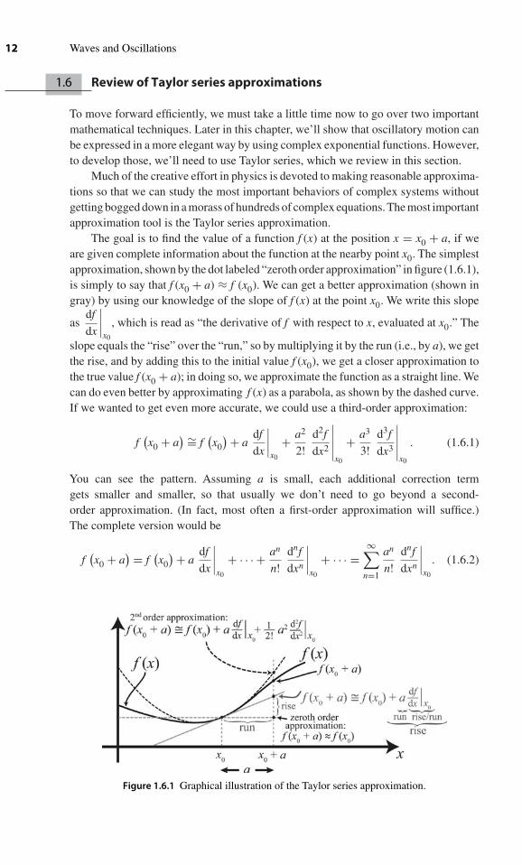
The goal is to find the value of a function f (x) at the position x = x0 + a, if weare given complete information about the function at the nearby point x0. The simplestapproximation, shown by the dot labeled “zeroth order approximation” in figure (1.6.1),is simply to say that f (x0 + a) ≈ f (x0). We can get a better approximation (shown ingray) by using our knowledge of the slope of f (x) at the point x0. We write this slope
asdf
dx
∣∣∣∣x0
, which is read as “the derivative of f with respect to x, evaluated at x0.” The
slope equals the “rise” over the “run,” so by multiplying it by the run (i.e., by a), we getthe rise, and by adding this to the initial value f (x0), we get a closer approximation tothe true value f (x0 + a); in doing so, we approximate the function as a straight line. Wecan do even better by approximating f (x) as a parabola, as shown by the dashed curve.If we wanted to get even more accurate, we could use a third-order approximation:
f(x0 + a
) ∼= f(x0
) + adf
dx
∣∣∣∣x0
+ a2
2!d2f
dx2
∣∣∣∣∣x0
+ a3
3!d3f
dx3
∣∣∣∣∣x0
. (1.6.1)
You can see the pattern. Assuming a is small, each additional correction termgets smaller and smaller, so that usually we don’t need to go beyond a second-order approximation. (In fact, most often a first-order approximation will suffice.)The complete version would be
f(x0 + a
) = f(x0
) + adf
dx
∣∣∣∣x0
+ · · · + an
n!dnf
dxn
∣∣∣∣x0
+ · · · =∞∑
n=1
an
n!dnf
dxn
∣∣∣∣x0
. (1.6.2)
Figure 1.6.1 Graphical illustration of the Taylor series approximation.

Chapter 1 ■ Simple Harmonic Motion 13
As an example, let’s find the Taylor series for the sine function:
f (θ) ≡ sin θ ⇒ df
dθ= cos θ,
d2f
dθ2= − sin θ,
d3f
dθ3= − cos θ,
d4f
dθ4= sin θ, . . .
Plugging this into equation (1.6.2), using θ as the variable instead of x, and expandingaround θ0 = 0 gives
sin θ = sin 0 + θ cos 0 + θ2
2! (− sin 0) + θ3
3! (− cos 0) + θ4
4! (sin 0) + θ5
5! (cos 0) + · · ·
⇒ sin θ = θ − θ3
3! + θ5
5! − · · · (1.6.3)
From this, we can see why the approximation
sin θ ∼= θ (θ in radians) (1.6.4)
works so well for small θ : there is no second-order correction term – the nextcorrection term is third order. (In fact, as you can show yourself on your calculator,this approximation works pretty well up to about θ = 0.4 radians = 23◦.)
Your turn: Show that
cos θ = 1 − θ2
2! + θ4
4! − · · · (1.6.5)
1.7 Euler’s equation
We will see in section 1.9 that there is a different way of expressing the solutionfor simple harmonic motion, x = A cos(ωt + ϕ), one which will become much moreconvenient when we begin treating more complicated systems. We will make use ofEuler’s equation:
eiθ = cos θ + i sin θ. (1.7.1)
Here, i ≡ √−1. The proof of this statement, and also the understanding of what itmeans to have a complex number as an exponent, comes through consideration ofseries expansions. Using the Taylor expansions we just derived for cos and sin, we canexpress the right side of this as
cos θ + i sin θ = 1 + iθ − θ2
2! − iθ3
3! + θ4
4! + · · · (1.7.2)
14 Waves and Oscillations
Now, we express the left side of equation (1.7.1) using a Taylor series, againexpanding around θ0 = 0:
eiθ = ei0 + θ iei0 + θ2
2! i2ei0 + θ3
3! i3ei0 + θ4
4! i4ei0 + · · ·
= 1 + iθ − θ2
2! − iθ3
3!+ θ4
4!+ · · ·
This is just the same as equation (1.7.2), which proves equation (1.7.1). This was firstdemonstrated by Leonhard Euler6 in 1748. You will use Euler’s equation every dayfor the rest of your life , so you are encouraged to commit it to memory.
1.8 Review of complex numbers
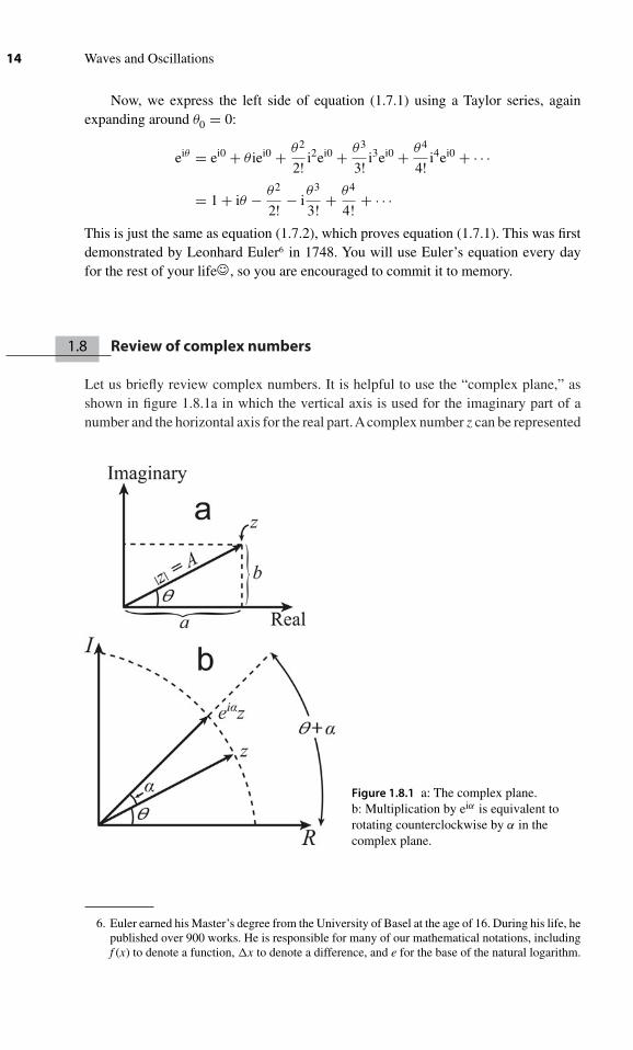
Let us briefly review complex numbers. It is helpful to use the “complex plane,” asshown in figure 1.8.1a in which the vertical axis is used for the imaginary part of anumber and the horizontal axis for the real part.Acomplex number z can be represented
Figure 1.8.1 a: The complex plane.b: Multiplication by eiα is equivalent torotating counterclockwise by α in thecomplex plane.
6. Euler earned his Master’s degree from the University of Basel at the age of 16. During his life, hepublished over 900 works. He is responsible for many of our mathematical notations, includingf (x) to denote a function, x to denote a difference, and e for the base of the natural logarithm.

Chapter 1 ■ Simple Harmonic Motion 15
as a vector in this plane, and we can write the “Cartesian representation” for the numberas z = a + ib. We see from the diagram that the length or magnitude of the vector isgiven by A = |z| = √
a2 + b2. Simple trigonometry then provides that
a = A cos θ and b = A sin θ, so that
z = a + ib = A cos θ + i(A sin θ) = Aeiθ
(using Euler’s equation) and also
θ = tan−1(b/a).
Your turn: If you’ve not already done so, read the aside about the arctan function insection 1.3. Then, explain why a more complete version of the above equation is
θ = tan−1 (b/
a) +
{0 if a > 0
π if a < 0
Let us collect all these useful relations into a single box:
z = a + ib “Cartesian representation”
– or –
z = Aeiθ “Polar representation,”
where
A = |z| =√
a2 + b2 and θ = tan−1(b/
a) +
{0 if a > 0π if a < 0
What happens in the complex plane when we multiply z by eiα?
eiαz = eiα Aeiθ = Aei(θ+α).
This is a vector in the complex plane which still has length A, but has been rotatedcounterclockwise by the angle α so that it now points in the direction given by θ + α,as shown in figure 1.8.1b. Thus,
Multiplying a number by eiα is equivalent to rotating its vector counterclockwise by α
in the complex plane.
Often we need to take the “complex conjugate” of a complex number:
To form the complex conjugate, simply replace every instance of i by −i.
For example, the complex conjugate of a+ib is just a−ib. We denote the complexconjugate with a star: the complex conjugate of z is z∗. As another example, if z = eiθ ,then z∗ = e−iθ . The complex conjugate is often used to calculate the magnitude of acomplex number. This is perhaps the easiest to see with a number expressed in polar
16 Waves and Oscillations
form: if z = Aeiθ (with A real), then z∗ = Ae−iθ , so that z∗z = A2 = |z|2. So, in general,we have
|z|2 = z∗z.
Finally, we introduce the notation for the real and imaginary parts of a complex number:
If z = a + ib, then Re z = a and Im z = b.
(Note that the i is not included in Im z.)
Self-test (answer below7): Show that, for any complex number z, Re z = Re(z∗) .
1.9 Complex exponential notation for oscillatory motion
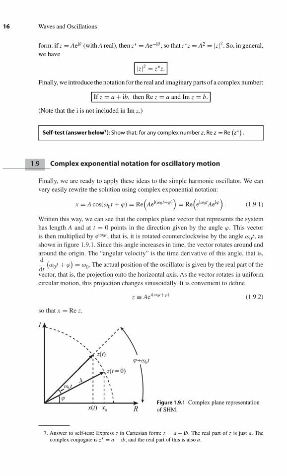
Finally, we are ready to apply these ideas to the simple harmonic oscillator. We canvery easily rewrite the solution using complex exponential notation:
x = A cos(ω0t + ϕ) = Re(
Aei(ω0t+ϕ))
= Re(
eiω0tAeiϕ)
. (1.9.1)
Written this way, we can see that the complex plane vector that represents the systemhas length A and at t = 0 points in the direction given by the angle ϕ. This vectoris then multiplied by eiω0t , that is, it is rotated counterclockwise by the angle ω0t, asshown in figure 1.9.1. Since this angle increases in time, the vector rotates around andaround the origin. The “angular velocity” is the time derivative of this angle, that is,d
dt
(ω0t + ϕ
) = ω0. The actual position of the oscillator is given by the real part of the
vector, that is, the projection onto the horizontal axis. As the vector rotates in uniformcircular motion, this projection changes sinusoidally. It is convenient to define
z ≡ Aei(ω0t+ϕ) (1.9.2)
so that x = Re z.
Figure 1.9.1 Complex plane representationof SHM.
7. Answer to self-test: Express z in Cartesian form: z = a + ib. The real part of z is just a. Thecomplex conjugate is z∗ = a − ib, and the real part of this is also a.

Chapter 1 ■ Simple Harmonic Motion 17
This method of portraying the motion brings out the physical significance of Aand ϕ more clearly. From figure 1.9.1, we can see that
ϕ = cos−1 x0
A, (1.9.3)
where x0 is the initial position. It is also clearer, perhaps, that A is related to the totalenergy of the system. From the discussion surrounding figure 1.2.1, we know that thepotential energy of a harmonic oscillator is given by
U (x) = 1
2kx2 + const.
Usually, it is convenient to choose the constant so that U(x) = 0 at the equilibriumposition x = 0, so that
U (x) = 1
2kx2. (1.9.4)
When x = A, the oscillator is at its maximum displacement, and so is momentarily atrest. Therefore, all the energy is in the form of potential energy, so that
E = 1
2kA2 ⇔ A =
√2E
k, (1.9.5)
where E is the total energy.It is also easy to show the relationships between position, velocity, and acceleration
using this complex plane picture. Take a moment now to convince yourself that theoperations of taking time derivatives and taking the real part of a quantity “commute,”that is, the order doesn’t matter, that is,
Redz
dt= d Re z
dt.
Therefore, we can write
x = Re z and x = Re z.
Plugging in for z from equation (1.9.2) gives
z = iω0z and z = −ω20z. (1.9.6)
Using Euler’s equation, we see that ei π2 = i, so that multiplication by i rotates a
complex plane vector counterclockwise by π/2. Equation (1.9.6) thus says that thecomplex plane vector representing the velocity, z, is rotated by a constant angle π /2“ahead” of the position vector z (and is scaled by the factor ω0). Similarly, since−1 = i · i, multiplication by −1 rotates a complex plane vector through 2 · (π/2) = π .Equation (1.9.6) thus says that z is always an angle π ahead of z (and is scaled byω2
0). These relationships are shown in figure 1.9.2; bear in mind that the position,velocity, and acceleration have different units, so the relative lengths of the vectors ineach picture are not meaningful. As shown in the upper left part of the figure, for theimportant special case of zero initial velocity, A = x0. We will use this result againlater.
This is a good time to point out that, although taking the real part does commutewith taking the derivative, addition, and multiplication by a real number, taking thereal part does not commute with multiplication by a complex number. For example,

18 Waves and Oscillations
Figure 1.9.2 Phase relationships for SHM. Top left: initial velocity = 0 shown for t = 0 . Topright: initial velocity = 0 shown for t > 0 . Bottom: Similar pictures for initial velocity <0.
if z1 = A1eiϕ1 and z2 = A2eiϕ2 , then Re[z1z2
] = Re[A1A2ei(ϕ1+ϕ2)
] = A1A2 cos(ϕ1 + ϕ2
),
whereas(Re z1
) (Re z2
) = A1A2 cos ϕ1 cos ϕ2. It is especially important to bear this inmind when calculating energies; for example, KE = 1
2 mx2 = 12 m (Re z)2 �= 1
2 mRe(z2).
1.10 The complex representation for AC circuits
In section 1.5, we discussed one type of electrical oscillator. However, there are manyother circuit examples in which the voltage and current vary sinusoidally in time.Such circuits are essential to the operation of virtually all analog (that is, nondigital)electronics, and the concepts involved in analyzing them are critical to the detailedunderstanding of all circuits. It is convenient to use a complex representation forthe currents and voltages in AC circuits, and this approach is used essentially by allscientists who work with circuits and essentially by all electrical engineers. So, thissection will provide a good chance to exercise the skills involving complex numbersthat we have just reviewed.
The simplest possibleAC circuit is shown in figure 1.10.1a. The signal generator onthe left of the circuit is a device that produces a voltage difference V0 cos ωt between itstwo terminals. In this circuit, it is connected to a resistor. Since only voltage differencesare physically important, we can define V ≡ 0 at any point in the circuit. For manyactual circuits, the V ≡ 0 point is ground (literally the voltage of the dirt under yourbuilding). For the rest of this section, we’ll use this convention; in the circuit shown, we

Chapter 1 ■ Simple Harmonic Motion 19
Figure 1.10.1 a: A signal generator (denoted by a sine waveinside a circle) connected to a resistor. b: Same circuit,drawn in the more conventional way using the groundsymbol. c: Complex representation for an AC voltage.
have grounded the lower terminal of the signal generator.Again, this does not affect theoperation of the circuit at all; it merely fixes the reference point with respect to whichvoltages are measured. The circuit can then be redrawn as shown in figure 1.10.1b; allpoints in the circuit with the ground symbol are connected together.
For a resistor, V = IR ⇔ I = V/R, so for this circuit I = V0
Rcos ωt.
Now, let’s apply the complex representation. The voltage is
V = V0 cos ωt = Re V , where V = V0eiωt
is the complex version of the voltage, as shown in figure 1.10.1c.8 Similarly, thecurrent is
I = V0
Rcos ωt = Re I, where I = V0
Reiωt .
Comparing this with the definition of V , we can write the complex version of Ohm’sLaw,
V = IZR,
where ZR = R is the “impedance” of the resistor. The impedance is a generalizedversion of the resistance; we will see below that it can be complex, so that we couldwrite it as |Z| eiϕ . Then, the general complex version of Ohm’s law would be
V = I |Z| eiϕ.
Since multiplying a complex number by the factor eiϕ rotates the complex plane vectorby angle ϕ, we see that the complex phase ϕ of the impedance is the phase differencebetween the current and the voltage. For a resistor, Z is real, so that the current and thevoltage are in phase, but we will see that, for inductors and capacitors, Z is imaginary,
8. We use the tilde (∼) above a symbol to indicate “complex version of,” so that V is the complexversion of V . Unfortunately, in many texts, V is simply written as V , and one must rememberthat, to find the actual voltage, one must take the real part.

20 Waves and Oscillations
Figure 1.10.2 a: A signal generator connected to acapacitor. b: An RC low-pass filter.
so that the current and voltage are not in phase, meaning that the sinusoidally varyingvoltage across a capacitor or inductor reaches a peak at a different time than thesinusoidally varying current flowing through it. (See problems 1.19, 1.22, and 1.23for more about these phase differences.) Note that the use of Z as a symbol for theimpedance is meant to tip you off that it may be a complex quantity, so it is conventionalnot to include the tilde over the Z .
So far, this is not terribly exciting. Things get more interesting when we introducea capacitor, as shown in figure 1.10.2a. We again use a signal generator to apply avoltage V0 cos ωt across the capacitor. This creates a time-dependent charge Q(t) onthe capacitor. To find the current, we use
Q = CVd/dt−−→ dQ
dt= C
dV
dt.
Since I = dQ
dt, we have
I = CdV
dt= C
d
dt
(V0 cos ωt
) = −CV0 ω sin ωt.
Now, let’s apply the complex representation. As before, we have
V = V0 cos ωt = Re V , where V = V0eiωt .
The current is
I = −CV0ω sin ωt = Re I, where I = iCV0 ωeiωt .
the complex version of Ohm’s Law in this case is
V = IZC,
where ZC is the impedance of the capacitor.
Your turn (answer below9): What is ZC in terms of C and ω?
9. ZC = V
I= V0eiωt
iCV0ωeiωt= 1
iωC.

Chapter 1 ■ Simple Harmonic Motion 21
To really see the power of this approach, we need to consider a more complicatedcircuit, such as that shown in figure 1.10.2b. No current is allowed to flow out of thecircuit at the point labeled VOUT ; instead, this is a place at which we will later calculatethe voltage. Again, we apply a voltage V0 cos ωt, this time to a series combination of aresistor and capacitor. What is the resulting current? It is related to the voltage acrossthe resistor by VR = IR, which is the real part of
VR = IZR. (1.10.1)
The total voltage across the series combination is the sum of the individual voltages:
VIN = VR + VC, which is the real part of
VIN = VR + VC ⇔ VR = VIN − VC ⇒ VR = VIN − IZC.
Substituting for VR from equation (1.10.1) gives
IZR = VIN − IZC ⇔ VIN = I(ZR + ZC
).
So, the total impedance is ZTOT = ZR + ZC, meaning that impedances in series add,just as one would expect from the behavior of resistors, i.e.,
Zseries = Z1 + Z2. (1.10.2)
In problem 1.20, you can show that impedances in parallel combine as one wouldexpect, that is,
1
Zparallel= 1
Z1+ 1
Z2. (1.10.3)
Core example: The low-pass filter. The circuit in figure 1.10.2b is one of the most usefuland common elements in analog circuitry. To understand why, let’s calculate VOUT:
VOUT = VC = IZC = VIN
ZTOTZC = VIN
ZC
ZR + ZC.
You may recognize this as the equation for a voltage divider; the fraction of the totalvoltage VIN that appears across the capacitor equals the fraction of the total impedancethat is due to the capacitor. Often, we are only interested in the amplitude of the outputvoltage expressed as a fraction of the amplitude of the input voltage. Recall that theamplitude of an oscillating quantity is the magnitude of the complex number thatrepresents it, as shown in figure 1.10.1c. Therefore,
amplitude of VOUT
amplitude of VIN=
∣∣∣VOUT
∣∣∣∣∣∣VIN
∣∣∣ .
You can show in problem 1.15 that, for any two complex numbers A and B,
∣∣∣∣AB∣∣∣∣ = |A|
|B| .
So,
amplitude of VOUT
amplitude of VIN=
∣∣∣∣VOUT
VIN
∣∣∣∣ =∣∣∣∣ ZC
ZR + ZC
∣∣∣∣ =∣∣ZC
∣∣∣∣ZR + ZC
∣∣ .continued

Referring to section 1.8, we see that
∣∣ZC
∣∣ =∣∣∣∣ 1iωC
∣∣∣∣ = 1ωC
and∣∣ZR + ZC
∣∣ =∣∣∣∣R + 1
iωC
∣∣∣∣ =√
R2 + 1
ω2C2 .
Therefore,
amplitude of VOUT
amplitude of VIN=
1ωC√
R2 + 1
ω2C2
= 1√ω2R2C2 + 1
= 1√1 +
(ω
ωLO
)2,
where
ωLO ≡ 1RC
.
The dependence of this ratio on the frequency of VIN is shown in figure 1.10.3. You cansee from these graphs, especially the log–log graph on the bottom, why this circuit iscalled a “low-pass filter.” If the angular frequency of VIN is well below ωLO, then theamplitude at the output is the same as the amplitude at the input, whereas if the angularfrequency of VIN is well above ωLO, then the output is dramatically smaller than the input.
Figure 1.10.3 Amplitude ratio for the low-pass filter shown in figure 1.10.2b. Top: linearaxes. Bottom: same data with log–log axes.
We can understand this behavior qualitatively, by remembering that the fractionof the input voltage that appears across the capacitor equals the fraction of the totalimpedance due to the capacitor. At low frequencies, the impedance of the capacitor islarge, so the fraction is nearly equal to 1, whereas at high frequencies the impedance ofthe capacitor is low, so the fraction approaches zero.
22

Chapter 1 ■ Simple Harmonic Motion 23
Finally, let us consider an inductor. We use the signal generator to apply a voltageV0 cos ωt = Re
(V0eiωt
)across the inductor. The magnitude of the voltage across the
inductor is
VL = LdI
dt⇔ dI
dt= VL
L
⇒ I = 1
L
∫VLdt = 1
L
∫V0 cos ωt dt = V0
Lωsin ωt + constant.
If the voltage amplitude V0 is zero, the current must be zero, so the constant must bezero. So,
I = V0
Lωsin ωt = Re I, where I = −i
V0
Lωeiωt,
since sin ωt = Re[−ieiωt
]. Thus, the impedance of the inductor is
ZL = V
I= V0eiωt
−iV0
Lωeiωt
= iωL.
Summarizing:
ZR = R ZC = 1
iωCZL = iωL. (1.10.4)
Concept test (answer below10): Does the circuit shown in figure 1.10.4 function
as a low pass filter (for whichamplitude of VOUT
amplitude of VIN= 1 for low frequencies and 0
for high frequencies), or instead does it function as a high-pass filter (for whichamplitude of V OUT
amplitude of V IN= 1 for high frequencies and 0 for low frequencies)? You
should be able to answer this question using qualitative reasoning, combined withequation (1.10.4).
Figure 1.10.4 An RL filter.
10. The output voltage divided by the input voltage equals the impedance of the resistor divided bythe total impedance. The impedance of the inductor is low for low frequency, meaning that mostof the total impedance is in the resistor, so VOUT ≈ VIN. On the other hand, at high frequencies,the impedance of the inductor is high, so the resistor represents a small fraction of the totalimpedance, and VOUT ≈ 0. So, this is a low-pass filter.

24 Waves and Oscillations
1.11 Another important complex function: The quantum mechanicalwavefunction
Our topics of study are waves and oscillations. However, one of the important reasonsfor mastering the concepts and techniques associated with these topics is that theyapply directly to quantum mechanics. Therefore, although we will not study quantummechanics per se in this book, we will point out some of the connections as we cometo them.
As you may know, small particles such as electrons display many wave-likeproperties. The wave nature of such a particle is described by the “wavefunction”� (the Greek capital letter psi). The wavefunction depends on both position and time,so we could write it as � (x, t), though usually we will simply write �. One of themost remarkable things about quantum mechanics is that � is inherently complex! Allthe information that can be known about the particle is contained in �, and in a latercourse you will learn how to extract from � quantities such as the momentum, angularmomentum, and energy. One aspect of � is relatively easy to understand: |� (x, t)|2is called the “probability density,” and is proportional to the probability of findingthe particle near the position x. For example, for the probability density shown infigure 1.11.1, the particle is likely to be found near x = −3 or 1 nm (1 nm = 10−9 m).This is called a “delocalized” wavefunction, since the particle might be found in twodifferent places. You’ll learn more about this in a later course.
Another example is that of an electron traveling at constant speed through avacuum; this is called a “free electron.” The wavefunction in this case is � (x, t) =ψ0e−iωteikx, where ψ0 (Greek lower case psi, with a naught subscript) is a constant,
k = ω
vpis called the “wavenumber,” and vp is the speed of the wave.11 This wavefunction
has an oscillatory dependence both on t and on x:
� (x, t) = ψ0e−iωteikx = ψ0 (cos ωt − i sin ωt) eikx = ψ0e−iωt (cos kx + i sin kx) .
Wavefunction for a free electron
This function is plotted in figure 1.11.2a and b.
Figure 1.11.1 A delocalized wavefunction.
11. The wavenumber k is also equal to 2π /λ, where λ is the “wavelength,” that is, the repeatinterval along the x-axis.

Chapter 1 ■ Simple Harmonic Motion 25
Figure 1.11.2 Real and imaginary parts ofthe wavefunction for an electron movingwith a constant velocity in a vacuum (i.e., a“free electron”). a: dependence on time ofthe wavefunction at x = 0. b: dependence onposition of the wavefunction at t = 0. c: Theprobability density is given by |�|2,showing that a free electron is completelydelocalized.
Self-test (answer below12): Show for � (x, t) = ψ0e−iωteikx that the probability density
|�|2 is equal to∣∣ψ0
∣∣2.
The result of this self-test is remarkable—there is no space or time dependence inthe probability density |�|2 for this case! This means that the particle is completelydelocalized—it is just as likely to be found at x = −100 nm as at x = +100 km, orat any other point, as shown in figure 1.11.2c. This waveform is an idealized version,since no real particle could be so infinitely spread out. However, real particles can behighly delocalized, even over macroscopic distances.
We will encounter � several more times in this text.
12. Answer to self-test: |�|2 = �∗� = (ψ∗
0 eiωte−ikx) (
ψ0e−iωteikx) = ψ∗
0 ψ0 = ∣∣ψ0
∣∣2

26 Waves and Oscillations
1.12 Pure sinusoidal oscillations and uncertainty principles
In real life, oscillations usually only last for a finite period of time. For example, wemight strike a piano key, hold it down for a short length of time (allowing the stringinside the piano to vibrate), and then release the key (which immediately stops thevibration). If we strike the key at t1 and release it at t2, the resulting vibration of aparticular point on the string might look as shown in figure 1.12.1.
It is important to realize that the waveform of figure 1.12.1 is not a pure sinusoidaloscillation, since it is not of the form (1.2.4): x = A cos(ωt + ϕ). Equation (1.2.4)describes an oscillation which goes on infinitely in time, stretching back in time tot → −∞, and forward in time to t → +∞. This is not merely a semantic distinction.We will see in our study of Fourier Analysis (chapter 8) that a function of the formshown in figure 1.12.1 can be created by adding together a very large number of puresinusoids, only one of which is at the angular frequency ω.
This means that, for a function such as that shown in figure 1.12.1, the angularfrequency is not “well-defined,” that is, the function cannot be characterized by asingle angular frequency. (If it could, we could write it as x = A cos(ωt + ϕ).) Wedon’t have to wait for chapter 8 to see this – we can develop a qualitative argumentnow that shows it. Imagine that we try to determine the frequency of the waveformshown in figure 1.12.1 by counting the number of times it crosses zero. (This, in fact, ishow frequencies are determined in most experiments, which usually rely on electronic“frequency counters.”) There are two zero-crossings per period. Therefore, if we define
N ≡ number of zero crossings and t ≡ t2 − t1,
Then,
T = t
(N/2)⇒ f = 1
T= N
2t.
However, in any real signal, the beginning and the end are not defined with absolutecrispness – there is always a question about exactly where we should begin countingthe zero-crossings and where we should stop. We’re only making a rough argumenthere, so let’s say that there’s an uncertainty of 1 in the value of N . In other words, we
can’t really be sure whether we should write f = N
2tor f = N + 1
2t. Thus, there is an
uncertainty in f :
f = N + 1
2t− N
2t= 1
2t.
Figure 1.12.1 Motion of one point on a piano string.

Chapter 1 ■ Simple Harmonic Motion 27
We have used simple arguments about a simple way of determining the frequency.However, more sophisticated arguments give the same qualitative results: the shorterthe time interval t, the greater the uncertainty in the frequency f . The moresophisticated arguments, which use a more careful definition of t and f , show
that f is always at least as big as1
4πt. This is for an ideal circumstance, where the
profile of the wave has an ideal shape. Of course, it is always possible to have a wavewith a less ideal profile, or to be sloppy in doing the measurements, so that in general
f ≥ 1
4πt⇔
f t ≥ 1
4π. (1.12.1)
Frequency–time uncertainty relationship
(valid for all types of waves and oscillations)
We can apply identical arguments to something (such as a wave on the surface of theocean) that oscillates as a function of x instead of as a function of t. A pure sinusoidaloscillation as a function of t can be written
y (t) = A cos(ωt + ϕ) ⇒
y (t) = A cos
(2π
Tt + ϕ
), (1.12.2)
where T is the repeat interval in time (the period). (Here, we use y (t) for the oscillatingfunction, to avoid confusion with the variable x which is used for the position in thenext equation. However, y (t) can stand for exactly the same types of things as we’vepreviously discussed, such as the position of an oscillating tree branch.) Similarly, wecan write a pure sinusoidal oscillation as a function of x as
y (x) = A cos
(2π
λx + ϕ
), (1.12.3)
whereλ is the repeat interval in space (the “wavelength”).We see that equations (1.12.2)and (1.12.3) are isomorphic. (Recall that this means that they are exactly the same,except that different symbols appear.) In the isomorphism t becomes x and T becomesλ. We can use exactly the same arguments that lead us to equation (1.12.1), but applythem to oscillations as a function of x instead. Since f = 1/T , this gives
(1
λ
)x ≥ 1
4π. (1.12.4)
Uncertainty relationship between inverse wavelength and position
(valid for all types of waves and oscillations)
The uncertainty relations (1.12.1) and (1.12.4) apply to any type of oscillation or wave,whether it is a simple harmonic oscillator or the quantum mechanical wavefunction.
One of the fundamental relations of quantum mechanics relates the energy Eof the particle to the frequency of oscillation of the wavefunction. (e.g., for a free

28 Waves and Oscillations
electron, the wavefunction is � (x, t) = ψ0e−iωteikx, and the frequency is f = ω
2π.)
This fundamental relation is
E = hf , (1.12.5)
where h = 6.6260690 × 10⁻³⁴ J s is called “Planck’s constant.” As you will learn ina later course, this relation comes from experimental results, and cannot be derivedfrom arguments based on classical physics. As you read through this text, bear in mindthat essentially everything we say about classical waves and oscillators applies to �
as well. In particular, essentially everything we say about the frequency of a classicaloscillator applies to the frequency of � as well, and that, by equation (1.12.5), thisfrequency is proportional to the energy of the particle.
Combining equation (1.12.5) with (1.12.1) gives
(E
h
)t ≥ 1
4π⇒
Et ≥ h
4π. (1.12.6)
This is called the “energy–time uncertainty principle.” It states that it is not possible toexactly determine the energy of a system if one can only observe it for a short time. Ifthe energy of a system cannot be precisely determined on short time scales, then this“energy–time uncertainty principle” requires that we modify our understanding of theconservation of energy to allow for “quantum fluctuations.” For example, it is possiblefor pairs of particles (one normal matter and one antimatter) to be spontaneously createdout of the vacuum, which requires a tremendous amount of energy (on a particle scale).These particles can exist only for a fleeting moment, and then annihilate with eachother, releasing the energy they had “borrowed” before anyone could notice it wasmissing! Perhaps surprisingly, the effects of these “virtual particles” can be observedexperimentally, for example through the Casimir effect.13
The other fundamental relation of quantum mechanics is
p = h
λ, (1.12.7)
where p is the momentum of the particle. As with equation (1.12.5), this relationcomes from experimental results, and cannot be derived from classical principles.
13. In the region between two metal plates, the density of virtual particles is lower than in the regionoutside the plates, resulting in a force that pushes the plates together. For more information, seePrecision Measurement of the Casimir Force from 0.1 to 0.9 μm, by U. Mohideen and AnushreeRoy, Phys. Rev. Lett. 81, 4549 (1998). A summary is available at http://focus.aps.org/v2/st28.html

Chapter 1 ■ Simple Harmonic Motion 29
Combining equation (1.12.7) with (1.12.4) gives
(p
h
)x ≥ 1
4π⇔
px ≥ h
4π. (1.12.8)
This is the more famous “Heisenberg uncertainty principle,” which states that it isnot possible to simultaneously determine a particle’s position and its momentum withabsolute precision. Both of these important quantum mechanical uncertainty relations(1.12.6) and (1.12.8) are direct consequences of attributing a wave nature to particlesand not the result of any other “quantum mechanical weirdness.”
Despite all the above arguments, we are very often in the situation where the timeinterval t is much, much longer than the period T . In such a case, the frequency isfairly well defined (i.e., f is small), and we need not worry much about the concernsraised in this section.
Concept and skill inventory for chapter 1
After reading this chapter, you should fully understand the following
terms:
Stable equilibrium (1.2)Hooke’s Law (1.2)DEQ (1.2)Simple Harmonic Motion (SHM) (1.2)Harmonic approximation (1.2)Amplitude, phase, frequency, angular frequency, period (1.2–1.3)Adjustable constants (1.2)Capacitor, inductor (1.5)Kirchhoff’s loop rule (1.5)Isomorphism (1.5)Taylor series (1.6)Euler’s equation (1.7)Complex plane (1.8)Magnitude of a complex number (1.8)Complex conjugate (1.8)Signal generator (1.10)Ground for electrical circuits (1.10)Complex version of Ohm’s Law (1.10)Impedance, as applied to electrical components (1.10)Low-pass filter (1.10)Log–log axes (1.10)Quantum mechanical wavefunction (1.11)Probability density (1.11)

30 Waves and Oscillations
Free electron (1.11)Wavenumber (1.11)Frequency–time uncertainty relation (1.12)Inverse wavelength – position uncertainty relation (1.12)Energy–time uncertainty relation (1.12)Heisenberg (momentum–position) uncertainty relation (1.12)
You should know what happens when:
A system described by the harmonic approximation is displaced from equilibrium andthen released (1.2–1.3)
A complex number is multiplied by eiα (1.8)An input voltage is applied to a low-pass filter (1.10)
You should understand the following connections:
Frequency, angular frequency, & period (1.2–1.3)Mass on a spring & an LC oscillator (1.5)Current in a circuit & charge on a capacitor; be able to tell whether I = q or instead
I = −q (1.5)Cosine representation & complex exponential representation for SHM (1.9)x & z (1.9)One-dimensional oscillation & rotation in the complex plane (1.9)V & V (1.10)
You should be familiar with the following additional concepts:
Dot notation for time derivatives (1.2)Angular frequency for a mass/spring (1.3)The frequency for SHM doesn’t depend on amplitude (1.3)Angular frequency for an LC oscillator (1.5)First-order Taylor series approximation for sin (1.6)Second-order Taylor series approximation for cos (1.6)Taking the real part doesn’t commute with multiplication by a complex number (1.9)Impedance of resistors, capacitors, and inductors (1.10)
You should be able to:
Check a proposed solution to a DEQ to determine if it’s correct and if there arerestrictions on the parameters (1.2)
Find the amplitude and phase given the initial position and velocity (1.3)Deal with the multi-valued aspect of the arctan function (1.3)Use the isomorphism between the mass/spring and the LC oscillator to quickly adapt
results from one system to the other (1.5)Given a function, create the Taylor series for it (1.6)Explain what it means to take the exponential of a complex number (1.7)

Chapter 1 ■ Simple Harmonic Motion 31
Go back and forth between Cartesian and polar representations for complex num-bers (1.8)
Find the magnitude of a complex number (1.8)Find the energy of an oscillator given either the spring constant and the amplitude or
the mass and the maximum velocity (1.9)
Calculate
∣∣∣∣VOUT
VIN
∣∣∣∣for any simple combination of resistors, inductors, and capacitors
(1.10)
In addition to all of the above, you should be able to combine the concepts
you’ve learned to address new situations.
Problems
Note: Additional problems are available on the website for this text.
Instructor: Ratings of problem difficulty, full solutions, and additional supportmaterials are available on the website.
1.1 What is the difference between a stable and unstable equilibrium? Giveexamples of each type of equilibrium from everyday life.
1.2 Plasma oscillations. To turn a gas into a “plasma,” one or more electronsmust be completely separated from each nucleus. This can be accomplishedby applying a very strong electric field (as in a spark or a lightning bolt), bythe absorption of ultraviolet light (as happens in the “ionosphere,” one of theupper layers of our atmosphere), or by heating to a very high temperature(as occurs in the sun). We will model a plasma as a “gas” of electronswith number density n. (In other words, there are n electrons per cubicmeter.) Each electron has charge -e and mass me. Occupying the samevolume is a gas of positively charged ions, each with charge +e. Becausethe ions were created by removing the electrons from neutral atoms, thenumber density of ions is also n. (In other words, there are n ions per cubicmeter.)
Consider a cube of plasma, with sidelength �. Somehow (e.g., by applyingan electric field), the electrons are all displaced a small distance x to the right.This creates a layer of negative charge on the right, and leaves behind a layerof positive charge on the left, as shown in figure 1.P.1. For simplicity, treateach of these layers as an infinite thin sheet of charge. The layers create anelectric field throughout the plasma, pointing to the right. This field exerts aforce to the left on the electrons filling the central region of the figure, andto the right on the ions. However, we’ll focus on the electrons because theyare so much lighter, and assume that the ions remain stationary.
When we turn off the original force that caused the displacement x ofthe cube of electrons, the electric field from the surface charge layerscauses the electrons to spring back toward the left. However, because oftheir finite mass, they overshoot the equilibrium position (corresponding to

32 Waves and Oscillations
Figure 1.P.1 Model for the ionosphere. The figureshows a cross-sectional view of a cube of sidelength �.The electrons are represented by the region that isshaded with down-slanting lines, while the positivecharges are represented by the region shaded withup-slanting lines. Elayers is the field due to the thinlayers of charge on the left and right surfaces.
displacement x = 0), move to the left of the ions, then are pulled back to theright, and so on, in an oscillatory motion. In this problem, you’ll calculatethe frequency of this oscillation.
(a) Explain why the field produced by the combination of the two charge
layers in the region between them is E = nex
ε0. (You may need
to refer back to your intro. E&M textbook. Remember that we’retreating the layers of charge as infinite sheets.)
(b) Explain why this leads to a restoring force on the electrons F =−n2e2�3
ε0x. (Remember that x � �, so that the total charge of
electrons that experiences the electric force is not significantlychanged by the small number in the displaced region x.)
(c) Explain why this means that the oscillation frequency is ω =√ne2
meε0. This is called the plasma frequency. Only radio waves with
frequencies significantly higher than this can propagate throughthe plasma. Lower frequency waves are instead reflected. Thus,AM radio waves (which are low frequency) can bounce off theionosphere, leading to very long transmission range under goodconditions (at night), whereas FM radio waves (higher in frequency)don’t bounce off the ionosphere, and so the transmission range ismuch more limited.
1.3 Derive equations (1.3.4a) and (1.3.4b) from the equations immediatelypreceding them.
1.4 Consider the potential energy described in problem 1.14. For low amplitudes,the motion of the object is well described by simple harmonic motion, sothat the period is independent of amplitude. However, once the amplitudegets high enough this is no longer true. As the amplitude increases, does the

Chapter 1 ■ Simple Harmonic Motion 33
period increase or decrease? Explain your reasoning thoroughly, and assumethat the amplitude is always less than π/β.
1.5 A particle of mass m moves in the potential energy U = αx2 + βx4, whereα and β are both positive. (a) What is the angular frequency of oscillationfor small amplitudes? (b) If the amplitude is increased far enough, one findsthat the angular frequency starts to depend on amplitude. Does the angularfrequency increase or decrease as the amplitude is increased? Explain yourreasoning.
1.6 We can rewrite equation (1.3.4a) to get ω0 = v0√A2 − x2
0
. This makes it seem
that ω0 depends on the amplitude and initial conditions. Explain this seemingcontradiction with equation (1.3.3).
1.7 Before doing this problem, read footnote 4 in section 1.3 about linearhomogeneous DEQs. Show that, as claimed in that footnote, A1 cos ω0t +A2 sin ω0t = A cos(ω0t + ϕ), with A =
√A2
1 + A22 and ϕ = tan−1
(−A2/A1
).
1.8 A mass sits on a platform which oscillates vertically in simple harmonicmotion at a frequency of 5 Hz. Show that the mass loses contact with theplatform when the amplitude exceeds 1 cm. (Assume g = 9.8 m/s2.) Hints:The mass loses contact with the platform if the downward acceleration ofthe platform exceeds g. To keep the math simple, choose a zero phase factor,i.e., choose x = A cos ω0t.
1.9 Home experiment (work with only one other student on this, and includehis/her name with your problem): The light emitted by a nonflatscreen TVmakes a good stroboscope. A given point on the screen is actually dark mostof the time; it is lit a small fraction of the time at a regular repetition rate,which we’ll call fTV. The object of this experiment is to measure fTV; I’lltell you that it’s either 30 or 60 Hz. As a very crude measurement, waveyour finger in steady oscillation in front of the screen at a rate of about 4Hz, for example. Your finger will block the light from the screen wherever ithappens to be when the screen flashes on. Roughly measure (as best you andyour partner can) the amplitude of your finger’s oscillation. Then measurethe separation between successive finger shadows at the point of maximumvelocity. Assume the motion is sinusoidal. Calculate the maximum velocityof the finger, given the amplitude and finger frequency. Put all of this togetherto find fTV. (Recall that you’re told that it’s either 30 or 60 Hz, so yourmeasurements need only be precise enough to get a rough answer whichallows you to determine which of these two possibilities is correct.)
1.10 Read the aside about the arctan function in section 1.3. Explain why a
more complete version of equation (1.3.4b) would be ϕ = tan−1
(−v0
ωx0
)+{
0 if x0 > 0π if x0 < 0
.
1.11 Before doing this problem, read footnote 4 in section 1.3 about linearhomogeneous DEQs. A particle far from the Earth feels the pull of gravity
F = −GMm
x2, where G is the gravitational constant, M the mass of the Earth,

34 Waves and Oscillations
m the mass of the particle, and x is the distance from the center of the Earth tothe particle. Assume that the particle moves along a straight line that passesthrough the center of the Earth, that gravity is the only force acting on it,and that for the time period we are considering the particle doesn’t touch thesurface of the Earth (i.e., that it’s out in space).
(a) Write a DEQ of motion for the particle. (As an example of whatI mean by a DEQ of motion, for the simple harmonic oscillator itwould be x + ω2
0x = 0.)(b) If x1 (t) is one solution of the DEQ and x2 (t) is another, is the
combination x1 + x2 necessarily a solution? Why or why not?
1.12 Analogy between a capacitor and a spring. (a) How is adding charge toa capacitor like compressing a spring? (b) Why is it that the inverse of Cisomorphic to k, rather than just C itself ?
1.13 In research-level theoretical physics, it is almost never possible to get anexact solution because of the complexity of the problems being considered.Therefore, it is essential to make appropriate approximations, so as to getphysical insight. TheTaylor series is central to many of these approximations.You have already seen two of the three most common applications of the
Taylor series: sin θ ∼= θ (for small θ) and cos θ ∼= 1 − θ2
2(for small θ).
In this problem, you will demonstrate the third of the three most commonapplications. Show that (1 + x)n ∼= 1 + nx for x � 1. (Note that this workswhether n is positive or negative, integer or fractional.)
1.14 The potential energy for a particular object is U (x) = −L cos βx, where Land β are both > 0. (This potential energy function is important in the studyof superconductivity.)
(a) Make a sketch of this potential energy from x = −2π
βto x = +2π
β.
Indicate the scale on the vertical axis.(b) The object has mass m and total energy ETOT = −L + G, where
0 < G � L. (The symbol “�” means “much less than.”) Add adashed line to your sketch indicating this total energy.
(c) At t = 0, the object is at x = 0. Show that its motion canbe approximated by a simple harmonic oscillation, and find theapproximate frequency of oscillation. Hint: recall that the Taylor
series expansion for cos θ is cos θ = 1 − θ2
2! + θ4
4! − · · · , so that
for θ �1, cos θ ∼= 1 − θ2
2! .
1.15 Let C1 and C2 be complex numbers. Show that
∣∣∣∣C1
C2
∣∣∣∣ =∣∣C1
∣∣∣∣C2
∣∣ . Reminder:∣∣C1
∣∣ means “magnitude of C1”1.16 For each of the following, express the quantity shown either in the
form a+ib (i.e., Cartesian representation) or in the form Aeiα (i.e., polarrepresentation), whichever you find easier for each part of the problem.

Chapter 1 ■ Simple Harmonic Motion 35
In case you might be confused by the way I’ve written things: “i 4.5” means“i times 4.5.”
(a) (3.2 + i 6.7) + (5.6 – i 4.5)(b) 6.1 ei 1.2 + 1.2 ei 1.7
(c) (3.2 + i 6.7)(5.6 – i 4.5)(d) (6.1 ei 1.2)(1.2 ei 1.7)(e) What point is this problem trying to get across?
1.17 Let z1 = 8eiπ/6and z2 = √2ei3π/4.
(a) Represent z1 and z2 in the complex plane.(b) Find the real and imaginary parts of z1 and z2.
Express each of the following in the form Aeiϕ , where A and ϕ arereal:
(c) z1 + z2(d) z3
1z22
1.18 A mass m = 10 kg is oscillating on a spring with k = 10 N/m with littledamping. The displacement of the mass can be described byx(t) = Re
{Ceiωt
}, where C =(1 – i) cm.
(a) What is the value of ω?(b) What is the amplitude of the motion?(c) The solution can also be expressed in the form x(t) = A cos(ωt +ϕ).
What is the value of ϕ ?(d) Describe the initial conditions of the motion, that is, specify the
position and velocity at t = 0. As for all numbers in physics (exceptdimensionless quantities) be sure to include units!
(e) Sketch two graphs, one of position versus time and the other ofvelocity versus time. Be sure to label both axes of each graphquantitatively.
(f) What is the energy of the oscillator?
1.19 For an RC low-pass filter (figure 1.10.2b), show that
∣∣∣∣VOUT
VIN
∣∣∣∣ drops by a
factor of 10 for each factor of 10 increase in ω, for ω � ωLO.1.20 Using methods similar to those leading to equation (1.10.2), show that the
complex impedances of two circuit elements in parallel combine in the wayspecified by equation (1.10.3).
1.21 A voltage V (t) = V0 cos ωt is applied across a capacitor with capacitanceC. (a) Without using a symbolic algebra program or graphing calculator,make a sketch with curves for both V (t) and I (t), showing two fullperiods of oscillation. Label your sketch quantitatively. (b) For a capacitor,does the current “lead” the voltage (meaning that the current reachesa peak before the voltage does), or does the voltage lead the current?(c) Using simple ideas about charging of the capacitor and the connectionbetween voltage and charge, explain why your answer to part (b) makessense.
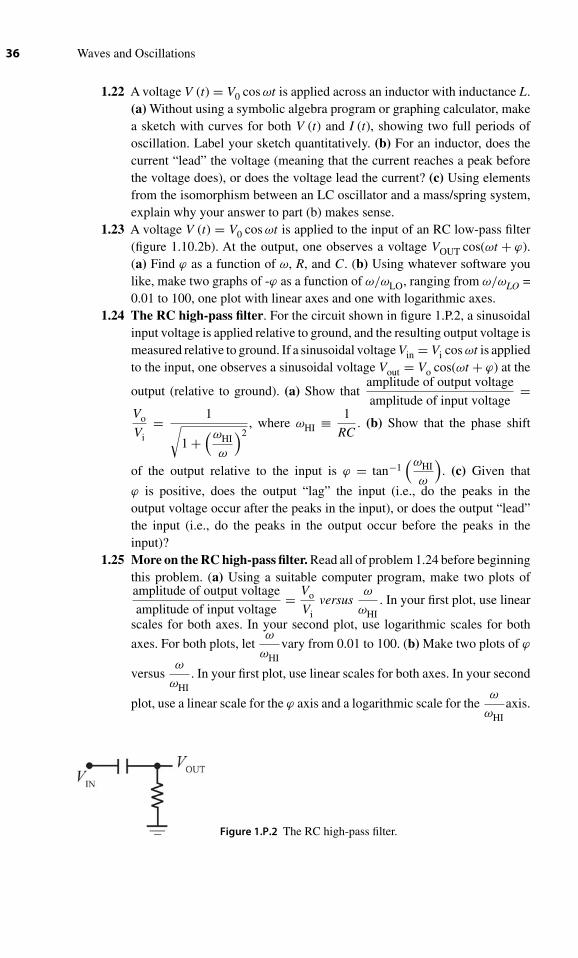
36 Waves and Oscillations
1.22 A voltage V (t) = V0 cos ωt is applied across an inductor with inductance L.(a) Without using a symbolic algebra program or graphing calculator, makea sketch with curves for both V (t) and I (t), showing two full periods ofoscillation. Label your sketch quantitatively. (b) For an inductor, does thecurrent “lead” the voltage (meaning that the current reaches a peak beforethe voltage does), or does the voltage lead the current? (c) Using elementsfrom the isomorphism between an LC oscillator and a mass/spring system,explain why your answer to part (b) makes sense.
1.23 A voltage V (t) = V0 cos ωt is applied to the input of an RC low-pass filter(figure 1.10.2b). At the output, one observes a voltage VOUT cos(ωt + ϕ).(a) Find ϕ as a function of ω, R, and C. (b) Using whatever software youlike, make two graphs of -ϕ as a function of ω/ωLO, ranging from ω/ωLO =0.01 to 100, one plot with linear axes and one with logarithmic axes.
1.24 The RC high-pass filter. For the circuit shown in figure 1.P.2, a sinusoidalinput voltage is applied relative to ground, and the resulting output voltage ismeasured relative to ground. If a sinusoidal voltage Vin = Vi cos ωt is appliedto the input, one observes a sinusoidal voltage Vout = Vo cos(ωt + ϕ) at the
output (relative to ground). (a) Show thatamplitude of output voltage
amplitude of input voltage=
Vo
Vi= 1√
1 +(ωHI
ω
)2, where ωHI ≡ 1
RC. (b) Show that the phase shift
of the output relative to the input is ϕ = tan−1(ωHI
ω
). (c) Given that
ϕ is positive, does the output “lag” the input (i.e., do the peaks in theoutput voltage occur after the peaks in the input), or does the output “lead”the input (i.e., do the peaks in the output occur before the peaks in theinput)?
1.25 More on the RC high-pass filter. Read all of problem 1.24 before beginningthis problem. (a) Using a suitable computer program, make two plots ofamplitude of output voltage
amplitude of input voltage= Vo
Viversus
ω
ωHI. In your first plot, use linear
scales for both axes. In your second plot, use logarithmic scales for both
axes. For both plots, letω
ωHIvary from 0.01 to 100. (b) Make two plots of ϕ
versusω
ωHI. In your first plot, use linear scales for both axes. In your second
plot, use a linear scale for the ϕ axis and a logarithmic scale for theω
ωHIaxis.
Figure 1.P.2 The RC high-pass filter.

Chapter 1 ■ Simple Harmonic Motion 37
For both plots, letω
ωHIvary from 0.01 to 100. (c) For ω � ωHI, show that
amplitude of output voltage
amplitude of input voltage= Vo
Vidrops by a factor of 10 for each factor of
10 decrease in ω.1.26 More on the RC low-pass filter. (a) Consider the RC low-pass filter shown
in figure 1.10.2b. If a voltage (relative to ground) Vin = Vi cos ωt is appliedto the input, one observes a sinusoidal voltage Vout = Vo cos (ωt + ϕ) at theoutput (relative to ground). Show that the phase shift of the output voltage
relative to the input is ϕ = tan−1
(− ω
ωLO
), where ωLO ≡ 1
RC. (b) Given
that ϕ is negative, does the output “lag” the input (i.e., do the peaks inthe output voltage occur after the peaks in the input), or does the output“lead” the input (i.e., do the peaks in the output occur before the peaks in theinput)?
1.27 The RL low-pass filter. One can use resistors and capacitors to build eitherlow-pass filters (see section 1.10) or high-pass filters (see problems 1.24and 1.25). It is also possible instead to use resistors and inductors forthese tasks; we’ll explore the low-pass version in this problem. In practicalcircuits, RC filters are much more common than RL filters, partly becauseit is easier to build an essentially ideal capacitor than to build an idealinductor. (There is always resistance in the wires used to wind an actualinductor, and there is always capacitance between the windings.) Also,inductors are generally bulkier and more expensive than the capacitorsthat could be used to build comparable filters. However, one does see RLfilters in some high frequency applications. Consider the circuit shown infigure 1.10.4. If a voltage (relative to ground) Vin = Vi cos ωt is applied tothe input, one observes a sinusoidal voltage Vout = Vo cos(ωt + ϕ) at the
output (relative to ground). (a) Show thatamplitude of output voltage
amplitude of input voltage=
Vo
Vi= 1√
1 +(
ω
ωLO
)2, where ωLO ≡ R
L. (b) Show that the phase shift of
the output relative to the input is ϕ = tan−1
(− ω
ωLO
). (Note that, except
for the definition of ωLO, these expressions are the same as for the RClow-pass filter.)
1.28 An electron in an atom can be excited from its original “ground state” toa well-defined and reproducible higher energy metastable “excited state.”The electron can then “fall” back down to the ground state, emitting aphoton in the process which has energy equal to the difference betweenthe ground state and the excited state. (As it turns out, this energy ischaracteristic of the type of atom, and so analysis of such photons can beused for determining the elements which are present in a sample.) Manyof these excited states have only a very short lifetime. For such a state,

38 Waves and Oscillations
if the experiment is performed carefully, one can determine that the photonsemitted from a large sample of material do not all have exactly the sameenergy, but instead there is a small spread. If a particular excited state hasa lifetime of 10−7 s, about how big a spread in photon energy would youexpect? Hint: Use the energy-time uncertainty relation; this is meant to bea very easy problem.

2 Examples of Simple Harmonic Motion
And I saw the cantilever jutting through the mist, resplendent in the light of dawn,oscillating jauntily like a promise of joy.
–Marian McKenzie
2.1 Requirements for harmonic oscillation
In this chapter, we will explore several examples of the remarkable variety of systemsthat show the harmonic oscillations described in chapter 1. There are two basicrequirements for a system to oscillate: (1) If the system is disturbed from equilibrium,there must be something (such as a force) that tends to bring it back toward equilibrium.For the oscillations to be of the sinusoidal form described in chapter 1, this restoringdrive must be proportional to the displacement from equilibrium, for example, thespring force F is proportional to x: F = −kx. (2) As the system moves towardequilibrium, there must be something (such as inertia) which tends to make the systemovershoot the equilibrium point.
Saying the same thing mathematically, if the system is described by a differentialequation of the form
F = −kx ⇒ md2x
dt2︸ ︷︷ ︸inertial term:satisfiescondition 2
= −kx︸︷︷︸restoring term:satisfiescondition 1
, (2.1.1)
then it will exhibit harmonic oscillations.Sometimes, it is easier to consider the energy of a system. If the system can be
described by an equation of the form
12 m
(dx
dt
)2
︸ ︷︷ ︸kineticenergy
+ 12 kx2︸︷︷︸
potentialenergy
= constant, (2.1.2)
then it will exhibit harmonic oscillation.
39

40 Waves and Oscillations
In other words, if we can show that a system obeys an equation either of the form(2.1.1) or of the form (2.1.2), then we can immediately conclude that
x = A cos(ω0t + ϕ
), where ω0 =
√k
m. (2.1.3)
2.2 Pendulums
Professor Roger Newton, author of the book Galileo’s Pendulum, recounts thiswonderful legend about Galileo, the world’s first experimental physicist, and arevelation that occurred during a church service in 1581:
He was seventeen and bored listening to the Mass being celebrated in the cathedral ofPisa. Looking for some object to arrest his attention, the young medical student beganto focus on a chandelier high above his head, hanging from a long, thin chain, swinginggently to and fro in the spring breeze. How long does it take for the oscillations to repeatthemselves, he wondered, timing them with his pulse. To his astonishment, he foundthat the lamp took as many pulse beats to complete a swing when hardly moving at allas when the wind made it sway more widely.1
This description of one of the first quantitative observations of experimental physicsshows the historic importance of pendulums in physics. We will see in chapter 4 thatpendulums provide an excellent illustration of chaos theory. Pendulums are commonin everyday life, from a baby’s swing to a grandfather clock, from a fair ride to awrecking ball.
We recognize Galileo’s observation that the period is independent of the amplitude,as a characteristic of simple harmonic motion. In the case of the pendulum, althoughthere is an obvious mass, there is no obvious spring. Yet, since it does have a position ofstable equilibrium, we should be able to model the potential energy near this positionas a parabola, and so we should be able to find an “effective spring constant” thatarises from the combination of gravity and the tension in the string.
Let’s consider an arbitrary rigid object of mass m that can rotate in the x–y planeabout a pivot P, as shown in figure 2.2.1. We’ll show that, for small amplitudes ofswing, the energy takes the form (2.1.2). In the figure, we displace the pendulum byan angle θ from equilibrium. The potential energy is determined by the position of thecenter of mass (marked CM in the figure): U = mgy, where y is the height of the CMabove its equilibrium position.
Your turn: Show that, if θ is small, then
U ∼= 12 mg �CM θ2. (2.2.1)
1. Roger G. Newton, Galileo’s Pendulum: From the Rhythm of Time to the Making of Matter,Harvard University Press, Cambridge, MA, 2004, p. 1.

Chapter 2 ■ Examples of Simple Harmonic Motion 41
Figure 2.2.1 A pendulum of arbitrary form.
Hint: Use the Taylor expansion for cos θ , which you derived in section 1.6:
cos θ = 1 − θ2
2! + θ4
4! − · · · (1.6.5)
( If θ is small, this means that cos θ ∼= 1 − θ2
2! .)
The motion is a pure rotation about P, so the kinetic energy is K = 12 Iω2, where
I is the moment of inertia for rotations about P and ω = θ is the angular velocity.Combining this with your result (2.2.1) gives the total energy:
E = U + K = 12 mg �CM θ2 + 1
2 I θ2 . (2.2.2)
Since the total energy is constant, this has exactly the same form as
(2.1.2) : 12 kx2 + 1
2 mx2 = constant,
so that we immediately know that the pendulum displays simple harmonic motion,that is, that
θ = θ0 cos(ω0t + ϕ
), where ω0 =
√mg �CM
I. (2.2.3)
Motion of a pendulum (mass need not be concentrated at a point).
I = moment of inertia about pivot, �CM = length from pivot to CM
Core example: the simple pendulum. The simplest example of a pendulum is a compactmass (the “pendulum bob”) at the end of a thin rod of length �; we assume the massof the rod is negligible compared to that of the bob. In this case, the moment of inertiaabout the pivot point is I = m�2. Plugging this into equation (2.2.3) gives
ωsimplependulum
=√
g
�. (2.2.4)

42 Waves and Oscillations
For more complicated objects, one often uses the parallel axis theorem, which youmay have seen proved in an introductory physics book:
I = ICM + mh2 , (2.2.5)
The parallel axis theorem
where ICM is the moment of inertia for rotations about the center of mass and h is thedistance from the pivot point P to the center of mass. By breaking a complicated objectup into smaller symmetrical objects and applying the parallel axis theorem, one cancompute I of the complicated object.
Although the harmonic motion of the pendulum is most easily seen by consideringthe time dependence of θ (as we have done earlier), we can also show that there is aharmonic variation in the horizontal position x. For a simple pendulum I = m�2, sothat equation (2.2.2) becomes
E = 12 mg�θ2 + 1
2 m�2θ2 = 12
mg
��2θ2 + 1
2 m�2θ2 = 12
mg
�(�θ)2 + 1
2 m
[d
dt(�θ)
]2
.
As we can see from the figure, in the limit of small displacements, the arc length �θ ∼= x,so that
E ∼= 12
(mg
�
)x2 + 1
2 mx2.
Since this has the same form as the energy of a mass/spring system, E = 12 kx2 + 1
2 mx2,
we see that the effective spring constant for the pendulum is kpendulum = mg
�. This
means that the net restoring force, which is created by a combination of gravity andthe string tension, is
Fpendulum = −kpendulum x = −mg
�x. (2.2.6)
“Pendulum force” resulting from the combination
of gravity and tension for a simple pendulum.
We will use this result again in chapter 5.
2.3 Elastic deformations and Young’s modulus
All materials are at least a little stretchy, although the amount an object can be stretchedbefore breaking is often too small to see with the naked eye. This stretchiness, andthe vibrations that occur when an object is stretched or twisted and then released,determine the engineering limits of building materials, the performance limits ofautomotive components, and the behavior of a new class of devices known as MicroElectroMechanical Systems (MEMS).2 In the remainder of this chapter, we’ll explore
2. These devices, which combine mechanical motion with electrical actuation or sensing, arefabricated using techniques of photolithography, electron beam lithography, and various types of

Chapter 2 ■ Examples of Simple Harmonic Motion 43
Figure 2.3.1 Top: a relaxed spring atits equilibrium length. Bottom: When
the spring is stretched, the left andright halves stretch by equal amounts.
various types of elastic (i.e., reversible) deformations, and their importance in scienceand everyday life.
The simplest way to deform an object is to stretch or compress it. Consider a longobject of uniform cross-section, such as a beam, which is anchored at the left end. Ifa force is applied to the right end, one always observes that the beam stretches by anamount proportional to the force. This comes as no surprise – before the force is applied,the beam is in equilibrium, and by the arguments in chapter 1 any displacement fromequilibrium is countered by a force Fspring = −kx. Therefore, to produce a displacementx, we must apply Fapplied = −Fspring = kx.
The spring constant k depends on the material from which the beam is made;diamond is stiffer than rubber. However, k also depends on the cross-sectional areaand length of the beam. We wish to divide out these geometric dependencies to geta parameter that describes the springiness or stiffness of the material itself. First, weconsider the dependence on length. How does k change if the beam is cut to half itslength? Since we’re modeling the beam as a spring, this is equivalent to asking whathappens to the spring constant of a spring when it is cut in half.
Imagine a spring of equilibrium length � which is attached to a wall on the left side.A dog pulls on the right end, stretching it by an amount�, as shown in figure 2.3.1.The force exerted by the spring on the dog is
Fby spring = −k �
⇔ k = − Fby spring
�= − Fby spring
extension. (2.3.1)
anisotropic (meaning directionally dependent) etching. The sizes of the devices range from thediameter of a human hair down to the molecular regime, allowing extremely fast response timesand, for devices designed to detect trace chemicals, extraordinary sensitivity. We will discussMEMS devices in sections 2.6 and 3.4. You can learn more about MEMS in problem 2.14, andin the website for this text, under the entry for this section.

44 Waves and Oscillations
The dog must be exerting an equal and opposite force k � on the right end of thespring. Since the right half of the spring doesn’t accelerate, we know there must beanother force to balance this; this force is exerted by the left half on the right half
Fby lefthalf
= −k �.
The extension of the left half is�
2. Therefore, by analogy with equation (2.3.1), the
spring constant of the left half is
klefthalf
= −F
by lefthalf
extension= − (−k �)
(�/2)= 2k.
Therefore, when a spring is cut in half, the spring constant gets doubled. (Another wayto see this: for the same extension, the coils of a short spring are distorted more thanthe coils of a long spring, therefore the shorter spring exerts a bigger force.)
Of course, this also means that, if the length of the spring (or in our case the length
of the beam) is doubled, the spring constant is halved. Thus, k ∝ 1
�. (The symbol ∝
means “proportional to.”)
Your turn (answer3 at bottom of page): Explain why k is proportional to the cross-sectional area A of the beam.
Putting these results together, we can write k ∝ A
�or
k = EA
�, (2.3.2)
where the proportionality constant E is called “Young’s Modulus,”4 and � is theequilibrium length of the beam.
We can also write
Fspring = −kx = −EA
�x ⇔ Fspring
A= −E
x
�.
The force applied to the beam, Fapplied, is equal and opposite to the force Fspring appliedby the beam, so that
Fapplied
A= E
x
�. (2.3.3)
3. Answer: We can divide the beam into N smaller beams running in parallel along the length. Theforce from a single one of these would be Fsmall = −ksmall x, where x is the amount by whichthe beam is stretched. The force from the entire beam is the total of the forces from the smallbeams: FTOT = NFsmall = − (
Nksmall
)x, so that the total spring constant is k = Nksmall. If the
cross-sectional area A is doubled, then N doubles, so k ∝ A.4. This is named after Thomas Young, who is most famous for his 1801 two-slit experiment, which
established the wave nature of light. Young was also a physician, and figured out how the eyefocuses on objects at different distances. He was familiar with twelve languages by the age offourteen, and later was involved in the translation of the Rosetta stone.

Chapter 2 ■ Examples of Simple Harmonic Motion 45
The quantity
σ ≡ F
A(2.3.4)
is called the stress. It is usually best to think of the F in this relation as being Fapplied.The stress has units of pressure; in SI units, 1 Pa (“Pascal”) = 1 N/m2. The quantity
ε ≡ x
�(2.3.5)
(the amount by which the beam stretches divided by its equilibrium length) is calledthe strain. Combining equations (2.3.3)–(2.3.5),
σ = Eε. (2.3.6)
In idiomatic English, the terms “stress” and “strain” are used in very similar ways,for example, “The stress of this job is killing me.” or, “I can’t stand the strain of thisresponsibility.” We can see above that, as used in physics and engineering, these arequite different quantities, with different units. The stress is usually best thought ofas something applied to the sample, while the strain is usually best thought of as theresponse of the sample to the stress. It might help you to remember that “stress” soundslike the first part of “pressure.”
Figure 2.3.2 shows a graph of strain versus stress for a typical metal beam.Rearranging equation (2.3.6) gives ε = σ/E, so that the slope of this graph is 1/E.For low stress, the graph is linear, as predicted by equation (2.3.6). However, oncethe stress becomes large enough, the beam no longer follows this relation. As shown,when the strain reaches the “elastic limit” (typically about 0.2% for metals), the springconstant decreases, then the beam “yields” and stretches a great deal with no additionalincrease in the applied stress. Then (again for metal beams), the microscopic structurechanges in a process called “strain hardening,” and finally the beam breaks. Table 2.3.1lists typical values of three important material parameters.
Figure 2.3.2 Strain vs. stress for a typical metal beam.

46 Waves and Oscillations
Table 2.3.1. Typical values of material parameters:
Material Young’s Modulus E Yield stress Shear Modulus G(109 N/m2) (106 N/m2) (109 N/m2)
Aluminum 75 300 28Brass 100 250 40Steel 200 400 75Concrete 20 40a
(compression only)Rock 50 100a
(compression only)Plastic 2 20 0.1Rubber 0.002 3 0.0005Wood 10 40Carbon nanotube 1000 60000
aThese materials do not exhibit yielding. The number quoted is the ultimate stress. i.e.the stress at breakage.
Self-test (answer below5): From table 2.3.1, we see that the values of E are a few hundredtimes larger than the values of the yield stress. How are E and the yield stress related?
Example: Scientists often need to isolate sensitive scientific equipment, such as atomicforce microscopes (AFMs), from building vibrations. An economical and effective way todo this is to place the equipment on a platform that is suspended on soft springs. As we’llsee in chapter 4, the effectiveness of this vibration isolation is best when the vibration
frequency of the system, ω0 =√
km is as low as possible. A scientist wants to suspend
an AFM of mass 5.4 kg (including the mass of the platform) using a rubber bungee cordof equilibrium length 1.2 m. If she wants ω0 = 10.0 rad/s, what is the required diameterfor the rubber cord? (Assume the mass of the cord is negligible compared to that ofthe AFM.)
Solution: ω0 =√
km ⇒ k = ω2
0m. Plugging in the numbers gives k = 540 N/m. From
equation (2.3.2), we have k = E A�
⇔ A = k�E . From table 2.3.1, the Young’s Modulus
for rubber is E = 0.002 × 10⁹ N/m2. Plugging in � = 1.2 m gives A = 3.2 cm2. SinceA = π
(d/2
)2, where d is the diameter, this gives d = 2.0 cm.The cord stretches a distance given by |F| = kx = mg ⇔ x = mg
k = 9.8 cm when theload is applied to it. The stress under load is approximately σ = mg
A = 1.6× 10⁵ N/m2,well below the yield stress.6
5. Answer to self-test: The yield stress is approximately equal to the Young’s modulus multipliedby the elastic limit, which is about 0.2%.
6. As the cord stretches, its cross-sectional area decreases somewhat, so this value for the stressis less than the true value. We can get a different estimate by assuming that the volume of thecord remains constant, so that A� = Astress (� + x) ⇔ Astress = A�
�+x , where Astress is the cross-
sectional area with the load applied. Plugging in the numbers gives Astress = 3.0 cm2, so that ournew estimate of the stress under load is σ = mg
Astress= 1.8× 10⁵ N/m2. This is greater than the
actual stress, because the volume actually increases when a beam (or in this case a bungee cord)

Chapter 2 ■ Examples of Simple Harmonic Motion 47
2.4 Shear
If we apply a force perpendicular to the face of a solid object, then it is stretched orcompressed, and the force over the area is the stress, as discussed in section 2.3. Theforce can be spread uniformly over the surface, resulting in a uniform pressure or stressσ = F/A. A force that is instead applied parallel to the face is called a shear force. Ifthis force is applied uniformly over the top surface of the cube shown in figure 2.4.1a,and this face has area A, then the shear stress is
σshear ≡ Fapplied
A. (2.4.1)
Figure 2.4.1 a: A force applied parallel to a face is called a shear force. For static equilibrium,forces must be applied to three other faces of the cube, as shown. This results in shear strain, asshown on the right. By imagining that we divide the cube into small parallel beams, such asthat shown shaded on the right, we can see that the force with which the cube resists the sheardeformation is proportional to the area of the top surface. b: Shear oscillations (side view).c: Front and back surfaces of a crystal from a quartz crystal microbalance, with gold electrodesapplied. Image from Wikimedia Commons.
is put under stress. For most materials, the volume increases by a fraction in the range ε/3 to ε/2.So, the correct value for σ is between this overestimate of 1.8 × 10⁵ N/m2 and the underestimateof 1.6 × 10⁵ N/m2 given in the main text above. For metal beams, the changes in volume and incross-sectional area are much smaller, and can often be ignored.

48 Waves and Oscillations
For static equilibrium to be achieved, this force to the right on the top surface mustbe balanced by an equal force to the left on the bottom surface. (Again, we assumethis force is applied uniformly over the surface.) However, this pair of forces wouldtend to rotate the cube clockwise. So, to provide zero net torque about the centerof the cube, we need forces on the left and right sides, as shown in figure 2.4.1a,and again we assume these are spread uniformly over the surface. This combinationof forces produces a condition of pure shear, resulting in the deformation shown inthe right side of figure 2.4.1a. If we imagine slicing the cube into thin horizontalslices, each slice is moved a little to the right of the one below it; this is called“shear strain.”
By now, it will not surprise you that the solid resists an applied shear force witha force F
springshear
= −kshearx. We can see from the figure that the displacement x is
proportional to the length �. Since kshear = −F
springshear
x= Fapplied
x, we see that kshear ∝
1
�. By the same arguments as in section 2.3, we could imagine dividing the solid
into smaller parallel beams, each of which resists the shear force, so that kshear ∝ A.
Combining these results, we get kshear ∝ A
�, or
kshear = GA
�, (2.4.2)
where the proportionality constant G is called the Shear Modulus.7
As in section 2.3, we can also write
kshear x = Fapplied ⇒ GA
�x = Fapplied ⇔ Fapplied
A= G
x
�.
We define the shear strain to be
γ ≡ x
�. (2.4.3)
Therefore,
σshear = Gγ. (2.4.4)
In addition to the shear modulus, we can also define the shear yield stress and theshear ultimate stress, which play roles analogous to those discussed in section 2.3. Thevalues of all three numbers are typically about half those of the corresponding numbersfor stretching/compression. (Some values are listed in table 2.3.1.)
Shear is particularly important in the design of earthquake-resistant buildings. Inmany earthquakes, there is a strong lateral oscillation of the ground, resulting in largeshear stress applied to the building. Buildings which are not specifically designed towithstand this type of stress are severely damaged by it.
7. This is named after William Shear (1701–1785), who also invented scissors. He received adoctorate from Oxford at the age of 14, and … OK, just kidding.

Chapter 2 ■ Examples of Simple Harmonic Motion 49
Since we can define a spring constant for shear, we see that an object can undergoshear oscillations, as shown in figure 2.4.1b. You can easily produce such oscillationsby placing a cube of jello on a plate and moving the plate sideways (simulating anearthquake).
Connection to current research: Quartz Crystal Microbalances
A piezoelectric material responds to an applied voltage by changing its shape. The mostcommercially important examples are quartz crystals (which exhibit a small but veryreproducible shape change) and lead zirconium titanate ceramics (which produce alarger but less reproducible change). In a quartz crystal microbalance (QCM), a quartzcrystal in the shape of a thin disk is prepared in such a way that it can be excited intoshear oscillations by the application of appropriate voltages to gold electrodes on thecrystal surface, as shown in figure 2.4.1c.
Because the mass is distributed through the thickness of the crystal, the quantitativeanalysis of these oscillations is beyond the level of this book. However, the frequency of
oscillation is given byω0 =√
keff
meff, where keff is an effective spring constant (proportional
to the shear modulus), and meff is an effective mass.The most common use for QCMs is for monitoring vacuum depositions of thin films.
For example, one might wish to coat a silicon wafer with a layer of copper, to formconnecting wires between micro-fabricated circuits. One can apply such a coating inseveral ways, including “thermal evaporation.” In this technique, the wafer is mountedface down in a vacuum chamber, and almost all the air is pumped out. Below thewafer, a pellet of copper is heated until it melts. Once the copper is liquid, it starts toevaporate. The thermal energy of the copper atoms that evaporate off the liquid is quitehigh so that they travel in straight lines until they strike the wafer. The thickness ofthe copper film thus applied to the wafer is measured using a QCM, which is mountedjust to the side of the wafer. The copper atoms coat the surface of the quartz crystal(as well as the silicon wafer), increasing its mass and thus changing ω0. This changecan be measured so accurately that it is routine to measure thicknesses down to oneatomic layer!
QCMs can also be used in aqueous solutions. Typically, the surface of the QCM sensorcrystal is first coated with a receptor chemical, such as the antibody for a particular virus.When the virus is introduced into the solution, it binds to the antibody resulting inan increase in the effective mass of the oscillating crystal. This technique can be usedto make sensors, to study the progress of chemical reactions, to sort through possibleanti-cancer drugs, and for many other applications.
2.5 Torsion and torsional oscillators
As a child, you probably played with a yo-yo, and had trouble with it when the stringgot twisted up. You may have held the top of the string, with the yo-yo resting at thebottom of the string, and watched it slowly untwist, picking up rotational velocity as

50 Waves and Oscillations
Figure 2.5.1 a: A yo-yo twisting onthe end of its string. b: Twisting athin-walled tube.
it went, as shown in figure 2.5.1a. You may have noticed that the yo-yo didn’t stoprotating when the string was untwisted, but instead kept rotating, twisting the stringin the other direction. Eventually, the yo-yo came to rest briefly before starting torotate in the opposite direction because of this new twist. Your yo-yo was acting asa torsional oscillator. As we’ll explore, more sophisticated versions have been veryimportant in the history of physics and continue to be important in current research onsuperfluids, supersolids, and other topics.
We begin by considering a thin-walled tube, as shown in figure 2.5.1b. Think ofit as a collection of thin strips, one of which is highlighted. We wish to calculate thepotential energy stored in this system when we twist it, and show that this has the formof the energy stored in a spring, U = 1
2 kx2. From there, we will be able to find theangular frequency of oscillation.
If we twist the top of the tube by a small angle θ , the strip experiences a shear
strain given bylateral displacement
length= x
�= rθ
�. Therefore, it produces a force
Fspringshear
= −kshearx = −kshearrθ.
Using equation (2.4.2): kshear = GA/� we then have
Fspring = −GAstrip
�rθ,
where Astrip is the cross-sectional area of the strip. The resulting torque is
τspringstrip
= rFspringshear
= −GAstrip
�r2θ.
To find the total torque from all the strips, we simply replace Astrip by the total cross-sectional area of the tube, A = 2πrt (valid for t � r), where t is the wall thickness ofthe tube:
τspringtube
= −2πGr3t
�θ. (2.5.1)

Chapter 2 ■ Examples of Simple Harmonic Motion 51
To create the twist, we must apply a torque of equal magnitude and opposite sign:
τapplied = 2πGr3t
�θ.
The work that we do in creating the twist is stored as potential energy. Recall fromyour earlier study of mechanics that the work done in a rotation is W = ∫
τ dθ , whichis analogous to the work done in a translation, W = ∫
F dx. Therefore,
U = Won system =θ∫
0
τapplied dθ = 2πGr3t
�
θ∫0
θ dθ = 12
(2πG
r3t
�
)θ2, (2.5.2)
which, as hoped, has the same form as the potential energy of a conventional spring.To complete our argument and find the angular frequency of oscillation, we must
consider the rotational kinetic energy. In most cases of interest, the object being twisted(the string of the yo-yo, or the tube) is used to support a much more massive object,such as the body of the yo-yo, which is called the rotor. For simplicity, we assume thatthe rotational kinetic energy of the rotor is much larger than that of the twisted elementthat supports it, so that
K = 12 Irotorω
2 = 12 Irotor
(dθ
dt
)2
.
Therefore, the total energy is
E = K + U = 12 Irotor
(dθ
dt
)2
+ 12
(2πG
r3t
�
)θ2. (2.5.3)
This is isomorphic to (i.e., is identical to except for a change of symbols)equation (2.1.2):
E = 12 m
(dx
dt
)2
+ 12 kx2,
so that we can rewrite ω0 =√
km for this case as
ωtubetorsion
=√
2πGr3t
Irotor�. (2.5.4)
In problem 2.12, you can show that, if the rotor is supported by a solid cylinder (e.g.,a wire or a string) instead of a tube, the torque and angular frequency of oscillation areinstead given by
τspringwire
= −πGr4
2�θ ω
wiretorsion
=√
πGr4
2Irotor�. (2.5.5)
Perhaps the most famous use of a torsional oscillator occurred in 1798, when HenryCavendish8 used one to measure the gravitational attraction between two pairs of lead
8. Henry Cavendish made important contributions to chemistry as well as physics. He was the first toisolate hydrogen gas, and showed that water is made from hydrogen and oxygen. He performed

52 Waves and Oscillations
Figure 2.5.2 Schematic diagram of the Cavendishexperiment. (Figure by Chris Burks.)
spheres, as shown in figure 2.5.2. The larger sphere in each pair was 1 ft (30.5 cm) indiameter, and the smaller was 2 in. (51 mm). To isolate the experiment from air currents,the instrument was housed inside a wooden box inside a specially built brick shed. Theoperation and observations could all be performed by Cavendish from outside the shed,using ropes, pulleys, and telescopes. To measure the gravitational interaction, he usedthe apparatus in “torsion balance” mode: he brought the large spheres close to the smallones, and measured how much the gravitational attraction caused the wire to twist; thiswas a static, not oscillating, experiment. However, to determine the torsional spring
constant of the wire (the quantityπGr4
2�in equation (2.5.5)), he moved the large balls
far away, and set the rotor (composed of the two small balls and the horizontal crossbarthat connects them) into oscillation. By measuring the resulting oscillation frequency,he could then deduce the spring constant.
Connection to current research: Torsional oscillators are used to investigate the phasetransitions of liquid helium to a superfluid and to a supersolid. See problem 2.13 tolearn more.
2.6 Bending and Cantilevers
When you jump on the end of a diving board, setting up a beautiful dive or anenthusiastic cannonball, you apply a force straight down. Although this is parallel
many important experiments on electricity, including a precise demonstration of the inversesquare law for the force between two charges, but never published most of his work. He was veryshy, especially around women; he communicated with his women servants via notes. His mainsocial outlet was attendance at scientific meetings. However, even once his scientific reputationwas well-established, he could sometimes be observed standing outside the door of a meeting,trying to work up enough courage to go in. He was fabulously wealthy; upon his death his estateamounted to nearly a million pounds sterling, a tremendous sum. (At that time, a gentlemancould live comfortably on 500 pounds a year.)
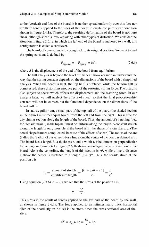
Chapter 2 ■ Examples of Simple Harmonic Motion 53
to the (vertical) end face of the board, it is neither spread uniformly over this face norare there forces applied to the sides of the board to create the pure shear conditionshown in figure 2.4.1a. Therefore, the resulting deformation of the board is not pureshear, although shear is involved along with other types of distortion. We consider thesituation in figure 2.6.1a, in which the left end of the board is anchored to a wall; thisconfiguration is called a cantilever.
The board, of course, tends to spring back to its original position. We want to findthe spring constant k, defined by
Fapplied = −Fspring = kd, (2.6.1)
where d is the displacement of the end of the board from equilibrium.The full analysis is beyond the level of this text, however we can understand the
way that the spring constant depends on the dimensions of the board with a simplifiedanalysis. When the board is bent, the top half is stretched while the bottom half iscompressed; these distortions produce part of the restoring spring force. The board isalso subject to shear, which affects the displacement and the restoring force. In ouranalysis later, we will neglect the effects of shear, so that the final proportionalityconstant will not be correct, but the functional dependence on the dimensions of theboard will be.
In static equilibrium, a small part of the top half of the board (the shaded sectionin the figure) must feel equal forces from the left and from the right. This is true forany similar section along the length of the board. Thus, the amount of stretching (i.e.,the “tensile strain”) in the top half must be uniform along the length. A constant stretchalong the length is only possible if the board is in the shape of a circular arc. (Theactual shape is more complicated, because of the effects of shear.) The radius of the arc(called the “radius of curvature”) for a line along the center of the board is defined as r.The board has a length L, a thickness t, and a width w (the dimension perpendicularto the page in figure 2.6.1). Figure 2.6.1b shows an enlarged view of a section of theboard. Along the centerline, the length of this section is rθ , while a line a distancez above the center is stretched to a length (r + z)θ . Thus, the tensile strain at theposition z is
ε = amount of stretch
equilibrium length= [(r + z) θ − rθ]
rθ= z
r.
Using equation (2.3.6), σ = Eε we see that the stress at the position z is
σ = Ez
r.
This stress is the result of forces applied to the left end of the board by the wall,as shown in figure 2.6.1a. The force applied to an infinitesimally thick horizontalslice of the board (figure 2.6.1c) is the stress times the cross-sectional area of theslice:
dF = σavw dz = Ez
rw dz.
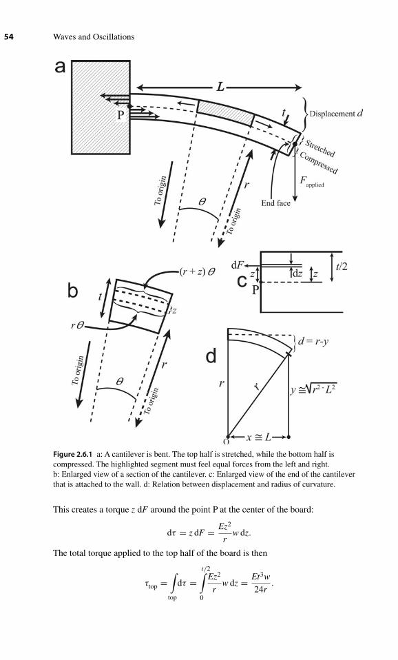
54 Waves and Oscillations
Figure 2.6.1 a: A cantilever is bent. The top half is stretched, while the bottom half iscompressed. The highlighted segment must feel equal forces from the left and right.b: Enlarged view of a section of the cantilever. c: Enlarged view of the end of the cantileverthat is attached to the wall. d: Relation between displacement and radius of curvature.
This creates a torque z dF around the point P at the center of the board:
dτ = z dF = Ez2
rw dz.
The total torque applied to the top half of the board is then
τtop =∫
top
dτ =t/2∫0
Ez2
rw dz = Et3w
24r.

Chapter 2 ■ Examples of Simple Harmonic Motion 55
A torque of the same magnitude arises from the forces applied to the bottom half, sothat the total torque around point P arising from the forces exerted by the wall is
τwall = 2τtop = Et3w
12r.
For static equilibrium, this must be equal in magnitude to the torque produced by theforce applied at the end of the board, Fapplied = kd. For small deflections, this torque is
τapplied = Fapplied L = kd L.
Equating the magnitudes of the torques gives
kd L = Et3w
12r⇔
k = Et3w
12rd L. (2.6.2)
Now, we must find the radius of curvature r in terms of the displacement d. Recall thatwe have approximated the shape of the bent board as a circle. We define the origin tobe at the center of the circle. The end of the board is at the position (x, y), where forsmall displacement x ∼= L. As we can see from figure 2.6.1d, the displacement is
d = r − y ∼= r −√
r2 − L2 = r − r
√1 − L2
r2.
For small displacements, the curvature is slight, that is, r � L. So, we can approximatethe square root using a Taylor series approximation:
√1 + x ∼= 1 + x/2 for x � 1.
Therefore,
d ∼= r − r
(1 − L2
2r2
)= L2
2r. (2.6.3)
Substituting this into equation (2.6.2) gives
k = Et3w
12rL2
2rL
= Et3w
6L3. (2.6.4)
The full analysis, including effects of shear, gives the exact result
kcantilever = Et3w
4L3. (2.6.5)
This is proportional to 1/L3; a factor of 1/L2 comes from the fact that the board iscurved, so that the displacement is geometrically proportional to L2 , equation (2.6.3).The third factor of L comes from the moment arm for the torque exerted by Fapplied.The spring constant is also proportional to t3w = t2 (tw). The first two factors of t comefrom the fact that the strain is proportional to the thickness, and from the moment armfor the force from the wall which provides the stress leading to this strain. The factor(tw) is the cross-sectional area of the board—a board with larger area of course has alarger spring constant.
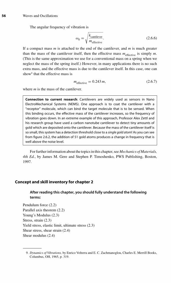
56 Waves and Oscillations
The angular frequency of vibration is
ω0 =√
kcantilever
meffective. (2.6.6)
If a compact mass m is attached to the end of the cantilever, and m is much greaterthan the mass of the cantilever itself, then the effective mass meffective is simply m.(This is the same approximation we use for a conventional mass on a spring when weneglect the mass of the spring itself.) However, in many applications there is no suchextra mass, and the effective mass is due to the cantilever itself. In this case, one canshow9 that the effective mass is
meffective = 0.243 m, (2.6.7)
where m is the mass of the cantilever.
Connection to current research: Cantilevers are widely used as sensors in NanoElectroMechanical Systems (NEMS). One approach is to coat the cantilever with a“receptor” molecule, which can bind the target molecule that is to be sensed. Whenthis binding occurs, the effective mass of the cantilever increases, so the frequency ofvibration goes down. In an extreme example of this approach, Professor Alex Zettl andhis research group have used a carbon nanotube cantilever to detect tiny amounts ofgold which are deposited onto the cantilever. Because the mass of the cantilever itself isso small, this system has a detection threshold close to a single gold atom! As you can seefrom figure 2.6.2, the addition of 51 gold atoms produces a change in frequency that iswell above the noise level.
For further information about the topics in this chapter, see Mechanics of Materials,4th Ed., by James M. Gere and Stephen P. Timoshenko, PWS Publishing, Boston,1997.
Concept and skill inventory for chapter 2
After reading this chapter, you should fully understand the following
terms:
Pendulum force (2.2)Parallel axis theorem (2.2)Young’s Modulus (2.3)Stress, strain (2.3)Yield stress, elastic limit, ultimate stress (2.3)Shear stress, shear strain (2.4)Shear modulus (2.4)
9. Dynamics of Vibrations, by Enrico Volterra and E. C. Zachmanoglou, Charles E. Merrill Books,Columbus, OH, 1965, p. 319.

Chapter 2 ■ Examples of Simple Harmonic Motion 57
Figure 2.6.2 Deposition of gold atoms onto a cantilever made from a carbon nanotube (shownschematically at the top) increases the mass of the cantilever, thus decreasing the vibrationfrequency (left vertical scale of the graph). During the shaded time periods (e.g. 60 s to 76 s),no atoms are deposited, so the frequency is constant. During the unshaded periods, atoms areadded, and the frequency decreases. Images Courtesy Zettl Research Group, LawrenceBerkeley National Laboratory and University of California at Berkeley.
Rotor (2.5)Cantilever (2.6)
You should know what happens when:
A spring is cut in half (2.3)
You should be able to:
Recognize by considerations of either force or energy when a system will oscillate,and be able to identify the effective mass and spring constant (2.1).

58 Waves and Oscillations
Calculate the oscillation frequency for any pendulum made up from symmetricalobjects (2.2)
Calculate the oscillation frequency for extension/compression (2.3), shear (2.4),torsional (2.5), and cantilever (2.6) oscillators
In addition to all of the above, you should be able to combine the concepts
you’ve learned to address new situations.
Problems
Note: Additional problems are available on the website for this text.
Instructors: Difficulty ratings for the problems, full solutions, and importantadditional support materials are available on the website.
2.1 True or False? If true, explain. If false, give a corrected version.If the net force on an object is zero at some position, and the object is
moved a short distance away and then released, it will then oscillate inharmonic motion.
2.2 The Sears Tower in Chicago was the tallest building in the world for 22 yearsand still holds the record for the highest antennas on top of a building. Thebuilding itself is 442 m high. The building sways considerably in the famouswinds of Chicago; on a typical day, the top floors sway laterally by up to15 cm, causing the toilets to slosh and occasionally giving people motionsickness. The total mass of the tower is 2.02 × 10⁸ kg. The average cross-sectional area is equivalent to a square 63 m on a side. If the tower is hit bya sudden gust of wind (which then suddenly stops), the tower is observed tosway back and forth with a period of 8 s. Model the building as a cantileverwith square cross-section (63 m on a side) and length of 442 m. (a) If wepretend the building is made from a uniform slab of material, what is theYoung’s modulus of this material? (b) You should have found a rather lowvalue, which is not surprising given that the volume of the Sears Tower ismostly air. To get a reasonable comparison, multiply your result by the ratioof the density of structural steel (7,850 kg/m3) to the average density of theSears Tower. You should still get a Young’s modulus which is considerablyless than that of steel, but this is reasonable since much of the weight of thetower does not contribute to its rigidity.
2.3 Radioactive materials emit three kinds of particles. When radioactivity wasfirst discovered, the identity of these particles wasn’t known, so they werenamed α, β, and γ particles. We now know that α-particles are helium nuclei,that is, two neutrons and two protons combined into a nucleus, β-particlesare electrons, and γ -particles are high-energy photons. In this problem, treateach of these as a point particle. An α-particle is fixed at the origin. Anelectron is fixed at x0 = 2.00 nm. (a) A negative fluorine ion is written F−.This is just a fluorine atom with an extra electron, and has essentially thesame mass as a fluorine atom. If the F− is placed at a position xeq, which

Chapter 2 ■ Examples of Simple Harmonic Motion 59
is to the right of x0, the total force on it is zero. What is the value of xeq?Treat all three particles as point charges. (b) Make a qualitative argumentfor why this is a position of stable equilibrium for the F−. (c) If the F− ismoved slightly from this position and then released, it oscillates. What is thefrequency of oscillation? (Hint: it is of order 1010 Hz. Begin by finding theeffective spring constant kspring. You are expected to find the mass of an Fatom by using the web or another reference source.)
2.4 You must do exercise 2.3 before doing this exercise. We allow the F− tomove relative to its equilibrium position xeq. (a) What is the potential energyfunction U(x) for the F−, assuming it is to the right of x = 2.00 nm? (SetU ≡ 0 at x = xeq.) (b) Using a suitable computer program, graph the potentialenergy for the F− over the x-range from xeq − 1 nm to xeq + 1 nm, andsuperimpose on this the graph of the harmonic (i.e., parabolic) approximationto this potential energy using your effective spring constant from exercise 2.3.
2.5 The Lennard–Jones Potential. Two neutral atoms have an attractiveinteraction due to a dynamic rearrangement of the electron clouds, called theVan der Waals attraction. It is frequently modeled using the Lennard–Jonespotential (proposed in 1924 by Sir John Lennard–Jones):
U (r) = 4ε
[(σ
r
)12 −(σ
r
)6]
,
where r is the distance between the two atoms and ε and σ are constants. Thisfunction is shown in figure 2.P.1. The positive term represents the repulsionexperienced at very short distances, which increases extremely rapidly asthe atoms are brought close together, while the negative term represents theattraction, which is more important at longer distances. (a) For what valueof r is the potential energy a minimum? (Express your answer in termsof σ .) (b) For the interaction of two argon atoms, ε = 1.654 × 10⁻²¹ J andσ = 3.405 Å, where 1 Å (pronounced “Angstrom”) is 10−10 m, and is namedafter Anders Ångström, one of the founders of spectroscopy. Assume thesenumerical values are exact. What is the value of U at the minimum in thiscase? (This is called the “bond energy” since it is the difference in potentialenergy between the bonded atoms and the situation with the atoms very farapart.) Quote your answer to six significant digits, and express your answerin electronvolts, where 1 eV= 1.60217653×10⁻¹⁹ J is the amount of energyan electron acquires as it moves through a voltage difference of 1 V.Atypical
Figure 2.P.1 The Lennard-Jones potential.

60 Waves and Oscillations
covalent bond has a bond energy of 2–4 eV, so we can see that Van der Waalsbonds are much weaker. (c) What is the value of U for an r which is 0.1 Ålarger than the minimum? (Again, express your answer in electronvolts, andquote to six significant digits.) (d) Using your numbers from parts (b) and(c), estimate the effective spring constant k for this system? (e) If the systemis displaced from equilibrium, by pulling the atoms further apart than theequilibrium distance you found in part (b) and then releasing them, bothatoms oscillate relative to the center of mass. This means that the center ofthe “spring” that connects them doesn’t move. So, you can picture this aseach atom oscillating on a spring half as long connected to a brick wall.Recalling that a spring half as long has twice the spring constant, what is thefrequency of oscillation? (You are expected to look up the mass of an Argonatom on the web or other reference source.)
2.6 What is wrong with the following reasoning: For a pendulum made froma thin rod, we can consider all the mass to be concentrated at the centerof mass. Therefore, the effective length is �/2, so the angular frequency is
ω0 =√
g
�/2=
√2g
�.
2.7 (a) If one wishes to make a pendulum with the longest possible period, howshould the mass be distributed along the length of the pendulum? Explainyour answer. (b) Your friend thinks it would be keen to make a pendulumwith a period of 1 h. Is this a practical idea? (Explain your reasoning.)
2.8 A pendulum is made from a light string that is 0.750-m long, with a smallbob of mass 0.500 kg at the end. The pendulum swings with an x-amplitudeof 5 cm. What is the energy present in this oscillation?
2.9 The tallest skyscraper (defined as having the highest occupied floor) in theworld is Taipei 101, in Taipei, Taiwan. The highest occupied floor is 439.2 mabove ground. A pendulum is suspended from this height (using a cantileverto get the support point out laterally away from the building). The pendulumis made from a steel rod that is 1 cm in diameter, with a 30-cm radius steelsphere attached at the bottom. The bottom of the sphere is 10 cm above theground. Assuming wind forces can be ignored, what is the period of thispendulum?
2.10 Assuming that wind forces can be neglected, what is the highest that one canmake a solid concrete tower of uniform cross-section (Take the density ofconcrete to be 2,400 kg/m3.)?
2.11 You are part of the design team for a manufacturer of air conditioning units.Aparticular large unit is to be mounted on four rubber feet, one at each corner.You are charged to decide on the size of these feet. The mass of the unit is1,000 kg. Its weight is equally distributed on the four feet. (a) What is theminimum area for each of the four feet? (Assume the yield stress for rubberin compression is the same as that in extension.) To play it safe, you decideon an area that is three times the minimum. (b) Your boss tells you, “We haveto be careful to avoid resonance with the frequency of the motors inside theunit.” (You’ll learn more about resonance in chapter 4.) She continues, “So,make sure the frequency of vertical oscillations is less than 5 Hz.” Does this

Chapter 2 ■ Examples of Simple Harmonic Motion 61
impose a minimum or a maximum limit on the thickness of the feet? (Assumethe mass of the rubber is negligible compared to that of the air conditioningunit.) Explain. (c) Based on what your boss has told you, choose a thicknessfor the feet. (d) If the air conditioning unit moves laterally in sinusoidalmotion, this imposes forces on the rubber that we will approximate as pureshear. What would the frequency of such oscillations be?
2.12 For a torsional oscillator, show that, if the rotor is supported by a solidcylinder (e.g., a wire or a string), the torque and angular frequency ofoscillation are given by
τspringwire
= −π Gr4
2�θ ω
wiretorsion
=√
π Gr4
2Irotor�.
(The rotor is assumed to have a much greater moment of inertia than thewire.)
2.13 Supersolid helium At very low temperatures, helium exhibits a variety ofastounding behaviors. At atmospheric pressure, helium gas liquefies whenthe temperature is reduced below 4.2 K. When the temperature is reducedbelow about 2 K, the liquid becomes a “superfluid” meaning that it has zeroviscosity, so that objects can move through it with zero drag. This effectwas demonstrated experimentally using torsional oscillators. Unlike all othermaterials, helium remains liquid all the way down to zero Kelvin, unless it isplaced under a pressure of at least 25 atmospheres. Above 25 atmospheres,it does become solid. In 2004, E. Kim and M. H. W. Chan (Science 305,1941–1944) used a torsional oscillator to demonstrate that, below about0.23 K the solid becomes a “supersolid,” which can flow without resistancein much the same way that the superfluid can. (It is difficult to conceive ofhow a solid could behave this way, but the experimental evidence is fairlyclear.) Figure 2.P.2 shows a schematic diagram of the torsional oscillator theyused. The rotor is suspended on a hollow tube made of beryllium–copper(BeCu), a very springy alloy. The tube has an inner diameter of 0.400 mm andan outer diameter of 2.20 mm. The rotor itself consists of a solid cylinder ofBeCu 12.8 mm in diameter and 5.00 mm high.Around this is a hollow annularregion that is filled with the helium, and around this is a hollow aluminumcylinder that has an inner diameter of 15.0 mm, an outer diameter of 17.0 mm,and a height that is also 5.00 mm.Adisk of BeCu that is 1-mm thick and has adiameter of 17.0 mm is attached to the top, and a second such disc is attachedto the bottom, sealing off the annular region between the BeCu cylinderand the aluminum cylinder. The annular region is filled with solid helium.Take the density of BeCu to be 8,350 kg/m3, that of aluminum to be 2,700kg/m3, and that of solid helium to be 172 kg/m3. Take the shear modulus ofBeCu to be 4.83 × 10¹⁰ N/m2. Assume all the preceding values are exact.Assume that the moment of inertia for the rotor assembly (including top andbottom caps, both cylinders, and the annular region filled with helium) ismuch larger than that of the BeCu tube from which it is suspended. (a) Whenthe helium is in the normal solid state, what is the oscillation frequency f for

62 Waves and Oscillations
Figure 2.P.2 Torsional oscillator used to detect the transition to supersolid helium.
this system, calculated to five significant figures? (Recall that the momentof inertia for a disk or solid cylinder is 1
2 MR2). (b) When the helium makesthe transition to the supersolid state, it no longer rotates along with therest of the rotor, so it doesn’t contribute to the moment of inertia. What isthe oscillation frequency under this condition, calculated to five significantfigures? (It was by detecting this change in oscillation frequency that Kimand Chan demonstrated the transition to supersolid helium.)
2.14 Micro ElectroMechanical Systems (MEMS). You are designing a sensorto detect biological pathogens in drinking water. Your sensor is based on acantilever which is micromachined from silicon, with a length of 300 μm, awidth of 100 μm, and a thickness of 1 μm. (Assume these dimensions areexact.) Because silicon is a crystal, the relevant value of Young’s modulusdepends on the direction relative to the crystal axes; assume it is exactly 165GPa for this problem. Assume the density of silicon is exactly 2,330 kg/m3.(a) What is the oscillation frequency f for your cantilever? (Give a resultwith eight significant figures, assuming all the numbers used as inputs areexact.) (b) You now coat your cantilever with a layer of receptor molecules,which can bind the pathogen. Each receptor molecule has a molecular weightof 278.1 u, where 1 u = 1.66053886 × 10⁻²⁷ kg. The receptor molecules

Chapter 2 ■ Examples of Simple Harmonic Motion 63
coat all the exposed surfaces of your cantilever, each occupying an averagearea of exactly (5 nm)2. Assume that this distributed mass counts towardthe effective mass in the same way that the mass of the silicon itself counts.What is the new oscillation frequency? (c) Each of the pathogens you mustdetect has a mass of 20,000 u. Assuming that 1% of the receptor moleculesbind a pathogen, what is the new oscillation frequency? (Again, assume thatthe distributed mass of the bound pathogens counts the same way that themass of the silicon itself counts.) (d) What is the minimum time for whichyou must make a frequency measurement to detect the difference betweenthe frequencies in parts (b) and (c)?

3 Damped Oscillations
Decay is inherent in all component things.Work out your salvation with diligence.
— The next-to-last thing said by the Buddha
3.1 Damped mechanical oscillators
Any real macroscopic oscillator that is displaced from equilibrium and released does notactually show the pure sinusoidal oscillations described in chapter 1; instead, the oscil-lations decay over time, as shown in figure 3.1.1. Fundamentally, this damping occursbecause a macroscopic oscillator is always coupled to its surroundings, even if weakly,and the energy initially present in the oscillation leaks away through these couplings.For example, the string of a violin is coupled to the body of the violin. If the stringis set into vibration, it causes the body to vibrate, which in turn sets the air vibratingand broadcasts sound waves, which carry away energy. The violin body also transmitsvibrations into the violinist, providing another channel for energy to leak away.
Following the approach of physics, we start by studying the simplest possible formof energy leakage: a drag force, also known as a “viscous damping force.” If you stickyour hand out of the window of a moving car, you feel the force of the air pushingagainst you. The force is opposite to the velocity of the car and increases the faster yougo. Thus, we might reasonably expect that the force of the air is
Fdrag = −bv, (3.1.1)
where b is a constant, and the minus sign shows that the force is in the opposite directionto the velocity.
Quantitative experiments with various objects show that equation (3.1.1) is correct,but only if the object is moving slowly enough that the airflow around it isn’t turbulent.The transition from nonturbulent or “laminar” flow at low speeds to turbulent flow athigher speeds can be visualized in a wind tunnel. In wind tunnel tests, it is easier to holdthe object fixed and blow the air past it, as shown in figure 3.1.2a. At low to moderatewind speeds, the air simply moves around the object, as shown in figure 3.1.2b. Athigher speeds, turbulent flow sets in, as shown in figure 3.1.2c, and the drag force isno longer described by equation (3.1.1). We will discuss the turbulent regime a littlemore in section 3.6.
64

Chapter 3 ■ Damped Oscillations 65
Figure 3.1.1 Decaying oscillations.
Figure 3.1.2 a: A stream of smoke isused to test the aerodynamics of a car in a
wind tunnel. The car is stationary, andlarge fans (not shown) force a flow of air
past it. The smoke flows smoothly overthe car without turbulence, indicating
laminar flow. This is desirable becauseit reduces air drag, improving fuel
efficiency. (Image courtesy of NASA.)b: A sphere in a wind tunnel. At lowspeeds, the airflow is laminar. c: Athigher speeds, the flow is turbulent.
For now, we focus on the laminar flow regime. It is important in its own right,and mathematically convenient. Further, many of the conclusions we will draw applyqualitatively to other energy leakage mechanisms. In this regime, the drag force isgiven by equation (3.1.1).
Now, we apply the same procedure as in chapter 1 to find the motion of a massexperiencing both a restoring force from a spring and a viscous damping force.
1. Write Newton’s second law for each object in the systemThere is only one object in this system, so we have
mx = FTotal ⇒ mx = −kx︸︷︷︸springforce
−bv︸︷︷︸viscousdamping
that is,
mx + bx + kx = 0 (3.1.2)
or
x + γ x + ω20x = 0, (3.1.3)

66 Waves and Oscillations
Figure 3.1.3 (decaying envelope) × (oscillating function) = decaying oscillation.
where
γ ≡ b
m(3.1.4)
characterizes the damping, and ω0 ≡√
km is the angular frequency of oscillations in
the absence of damping (i.e., in the absence of a drag force).Following the lead of chapter 1, we now cast the problem into complex form.
Equation (3.1.3) is the real part of
z + γ z + ω20z = 0, (3.1.5)
where z may be complex. If we can find a solution to equation (3.1.5), we automaticallyget a solution to equation (3.1.3) by setting x = Re z (since the operation of taking thereal part commutes with taking derivatives).
2. Use physical and mathematical intuition to guess a solutionAs suggested in figure 3.1.3, the solution might be of the form
x = [decaying envelope function] × A0 cos(ωvt + ϕ),
where ωv is the angular frequency in the presence of viscous damping (to bedetermined). It is not clear what the mathematical form of the decaying envelopefunction should be. However, we can start by trying a decaying exponential, since thisis easy to handle mathematically.1 So, we’ll try
[decaying envelope function] ?= e−σ t, (3.1.6)
1. We could instead try to guess the envelope function from energy considerations. Since Work =Force × distance, Power = Force × velocity. Therefore, the power dissipated by the dampingforce is P = Fdampv = −bv2. The average power over a cycle is then given by Paverage = 〈P〉 =⟨
dEdt
⟩= −b
⟨v2⟩, where the angle brackets indicate the average over a cycle. Let us assume for
now that the damping is relatively light. Then, the velocity will vary approximately sinusoidallyover a single cycle. The average value of the square of a sinusoid is exactly half the maximumof the square, as you can show by integration in problem 3.4. Therefore,
⟨v2⟩ = 1
2 v2max = E/m

Chapter 3 ■ Damped Oscillations 67
where the constant σ is to be determined. So, our complete guess is
x?= e−σ tA0 cos
(ωvt + ϕ
) = Re (z) ,
where z = A0e−σ tei(ωvt+ϕ) (3.1.7)
3. Plug the guess back into the differential equation to see if it is indeed asolution, and whether there are restrictions on the parameters.Let’s prepare to plug equation (3.1.7) into (3.1.5) by computing the derivatives:
z = A0eiϕe(−σ+iωv) t,
z = (−σ + iωv
)z,
z = (−σ + iωv
)2z.
Plugging into equation (3.1.5), z + γ z + ω20z = 0, gives(−σ + iωv
)2z + γ
(−σ + iωv
)z + ω2
0 z = 0.
Cancelling the z’s gives(−σ + iωv
)2 + γ(−σ + iωv
) + ω20 = 0,
⇒ σ 2 − i2σωv − ω2v − γ σ + iγωv + ω2
0 = 0.
This is actually two equations; the real part of the left side must equal the real part ofthe right side, and also the imaginary part of the left side must equal the imaginary partof the right side. So,
imaginary part: − 2σωv + γωv = 0 ⇒ σ = γ
2
(since E = 12 mv2
max). Plugging this in yields⟨dE
dt
⟩= −b
E
m⇒
⟨dE
dt
⟩= −γ E. (3.1.8)
If we restrict ourselves to timescales much longer than one period, we can write this as
dE
dt= −γ E ⇒ dE
E= −γ dt
Integrating both sides gives ln E = −γ t + const. ⇒ E = e-γ t+const. = econst.e−γ t . SettingE (t = 0) ≡ E0, we can identify the constant, so that
E = E0 e−γ t . (3.1.9)
The damping force does not affect the potential energy, so we still have U = 12 kx2 ⇒ E = 1
2 kx2max.
Combining this with equation (3.1.9) gives xmax =√
2Eok e− γ
2 t . This is of the same form asequation (3.1.6).

68 Waves and Oscillations
(in agreement with footnote 1 about guessing the envelope function from energyconsiderations), and
real part: σ 2 − ω2v − γ σ + ω2
0 = 0.
Substituting for σ gives
γ 2
4− ω2
v − γ 2
2+ ω2
0 = 0 ⇒
ωv =√
ω20 − γ 2
4. (3.1.10)
Thus, our guess
z = A0e− γ2 tei(ωv t+ϕ). (3.1.11)
is indeed a solution, but only if equation (3.1.10) is satisfied. This means that x isgiven by
x = Re (z) = A0e− γ2 t cos
(ωvt + ϕ
). (3.1.12)
Note that ωv is smaller than ω0, as shown by equation (3.1.10). This is perhapsintuitively reasonable, since the viscous damping slows down the oscillating mass.However, for most cases of practical interest, the difference between ωv and ω0 issmall, as we’ll explore further in section 3.4. The adjustable constants A0 and ϕ aredetermined by the initial position and velocity, as you can explore in problem 3.7.
3.2 Damped electrical oscillators
In section 1.5, we analyzed an LC oscillator. Now, we add a damping element to thecircuit: a resistor, as shown in figure 3.2.1. Air drag converts mechanical energy intothermal energy; a resistor converts electrical energy into thermal energy. The voltagesacross the capacitor and inductor are
VC = q
C(1.5.1) and VL = Lq. (1.5.6).
The magnitude of the voltage across the resistor is given by Ohm’s Law:∣∣VR
∣∣ = IR.We go clockwise around the loop when evaluating voltage changes, and we also define
Figure 3.2.1 Damped electricaloscillator.

Chapter 3 ■ Damped Oscillations 69
positive current to be clockwise. Since the voltage drops across the resistor, VR = −IR.As in section 1.5, positive Idecreases the charge on the capacitor, so I = −q. Therefore,
VR = −IR = qR.
Kirchhoff’s loop rule (which says that the sum of the voltage changes around a loopmust be zero) then gives
VL + VR + VC = 0 ⇒
Lq + Rq + 1
Cq = 0. (3.2.1)
This is isomorphic to (i.e., identical to except for a change of symbols) (3.1.2):
mx + bx + kx = 0.
Therefore, we simply change symbols in the solution (3.1.12):
q = A0e− γ2 t cos
(ωvt + ϕ
), (3.2.2)
where, as before, ωv =√
ω20 − γ 2
4 .
Your turn (answer2 below): Explain why, for the electrical oscillator, γ ≡ R
Land
ω0 ≡√
1LC
.
3.3 Exponential decay of energy
The solution for the damped mass/spring is
(3.1.12) : x = A0e− γ2 t cos
(ωvt + ϕ
).
If the damping is relatively light, then γ is small, and the amplitude of oscillationschanges only slowly. In this limit, we can say that the amplitude of oscillation is
A = A0 e− γ2 t, (3.3.1)
so that, within each cycle the potential energy reaches a maximum value of
Umax = E tot = 12 kA2 = 1
2 kA20e−γ t
⇒ E tot = E0e−γ t, (3.3.2)
where the initial energy is E0 = 12 kA2
0. This gives us a more direct interpretation of γ :in a time γ −1, the energy is reduced by a factor 1/e.
2. Comparing equation (3.1.2) with (3.2.1), we see that m becomes L, b becomes R, and k becomes
1/C. Making these substitutions into γ ≡ b/m and ω0 ≡ √k/m gives γ ≡ R
L and ω0 ≡√
1LC .

70 Waves and Oscillations
Concept test (answer3 below): Although the energy decays by a factor 1/e in a timeγ −1, according to equation (3.3.1) it takes a time 2γ −1 for the amplitude to decay bya factor 1/e. How can the energy decay more quickly than the amplitude?
Self-test (answer4 below): How long does it take for the energy to decay to 1% ofits initial value? Express your answer in terms of γ −1.
3.4 The quality factor
In virtually all circumstances, whether in science or engineering, people don’t specifythe degree of damping by providing a value for the b that appears in Fdamp = −bv, orfor γ ≡ b/m. Instead, they quote the quality factor Q:
Q ≡ ω0
γ. (3.4.1)
Since ω0 and γ both have units of s−1, this is a dimensionless number. It is a ratio ofthe rate of oscillations to the rate of energy loss through damping. A system with lowdamping has a low value of γ , and therefore a high Q.
High Q ⇔ low damping
For many applications, a large Q is desirable, because one often wants the oscillationto persist for a long time. Also, a large Q means that the decay of oscillations is slow, sothat the actual waveform is close to a perfect sinusoid, allowing for the most accuratetiming. In a good watch, the time is determined by counting the vibrations of a quartzcrystal having a Q of about 105. (The crystal is often in the shape of a tuning fork,as shown in figure 3.4.1. The usual oscillation frequency is 32,768 Hz = 215 Hz. It iseasy in digital circuitry to divide a frequency into half. Doing this 15 times results ina frequency of 1 Hz, which can be used to drive the second hand of the watch.)
However, in other applications, a low Q is preferable. For example, when thesuspension of a car is set into oscillation by driving over a pothole, the occupantswould prefer that it not keep oscillating for a long time! The suspension of a typicalcar has a Q of about 1.
3. Since E = 12 kA2, the amplitude need only decrease by a factor of
√2 in order for the energy to
decrease by a factor of 2.4. ln (100) γ −1 ∼= 4.6γ −1.
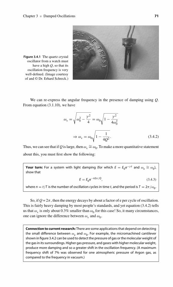
Chapter 3 ■ Damped Oscillations 71
Figure 3.4.1 The quartz crystaloscillator from a watch must
have a high Q, so that itsoscillation frequency is very
well-defined. (Image courtesyof and © Dr. Erhard Schreck.)
We can re-express the angular frequency in the presence of damping using Q.From equation (3.1.10), we have
ωv =√
ω20 − γ 2
4= ω0
√1 − γ 2
4ω20
⇒ ωv = ω0
√1 − 1
4Q2. (3.4.2)
Thus, we can see that if Q is large, then ωv∼= ω0. To make a more quantitative statement
about this, you must first show the following:
Your turn: For a system with light damping (for which E = E0e−γ t and ωv∼= ω0),
show that
E = E0e−n2π/Q, (3.4.3)
where n = t/T is the number of oscillation cycles in time t, and the period is T = 2π/ω0.
So, if Q = 2π , then the energy decays by about a factor of e per cycle of oscillation.This is fairly heavy damping by most people’s standards, and yet equation (3.4.2) tellsus that ωv is only about 0.3% smaller than ω0 for this case! So, it many circumstances,one can ignore the difference between ωv and ω0.
Connection to current research: There are some applications that depend on detectingthe small difference between ωv and ω0. For example, the micromachined cantilevershown in figure 3.4.2 can be used to detect the pressure of gas or the molecular weight ofthe gas in its surroundings. Higher gas pressure, and gases with higher molecular weight,produce more damping and so a greater shift in the oscillation frequency. (A maximumfrequency shift of 7% was observed for one atmospheric pressure of Argon gas, ascompared to the frequency in vacuum.)
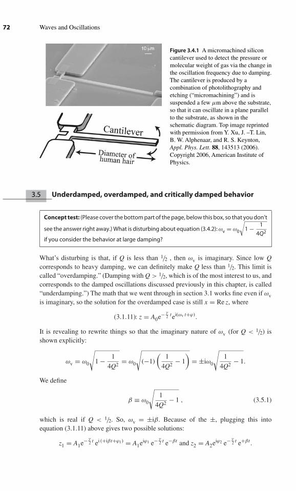
72 Waves and Oscillations
Figure 3.4.1 A micromachined siliconcantilever used to detect the pressure ormolecular weight of gas via the change inthe oscillation frequency due to damping.The cantilever is produced by acombination of photolithography andetching (“micromachining”) and issuspended a few μm above the substrate,so that it can oscillate in a plane parallelto the substrate, as shown in theschematic diagram. Top image reprintedwith permission from Y. Xu, J. –T. Lin,B. W. Alphenaar, and R. S. Keynton,Appl. Phys. Lett. 88, 143513 (2006).Copyright 2006, American Institute ofPhysics.
3.5 Underdamped, overdamped, and critically damped behavior
Concept test: (Please cover the bottom part of the page, below this box, so that you don’t
see the answer right away.) What is disturbing about equation (3.4.2): ωv = ω0
√1 − 1
4Q2
if you consider the behavior at large damping?
What’s disturbing is that, if Q is less than 1/2 , then ωv is imaginary. Since low Qcorresponds to heavy damping, we can definitely make Q less than 1/2. This limit iscalled “overdamping.” (Damping with Q > 1/2, which is of the most interest to us, andcorresponds to the damped oscillations discussed previously in this chapter, is called“underdamping.”) The math that we went through in section 3.1 works fine even if ωvis imaginary, so the solution for the overdamped case is still x = Re z, where
(3.1.11): z = A0e− γ2 tei(ωv t+ϕ).
It is revealing to rewrite things so that the imaginary nature of ωv (for Q < 1/2) isshown explicitly:
ωv = ω0
√1 − 1
4Q2= ω0
√(−1)
(1
4Q2− 1
)= ±iω0
√1
4Q2− 1.
We define
β ≡ ω0
√1
4Q2− 1 , (3.5.1)
which is real if Q < 1/2. So, ωv = ±iβ. Because of the ±, plugging this intoequation (3.1.11) above gives two possible solutions:
z1 = A1e− γ2 t ei (+iβt+ϕ1) = A1eiϕ1 e− γ
2 t e−βt and z2 = A2eiϕ2 e− γ2 t e+βt .

Chapter 3 ■ Damped Oscillations 73
As discussed in footnote 3 of section 1.3, the general solution of a linear, homogeneoussecond order differential equation, such as the differential equation (3.1.5): z + γ z +ω2
0z = 0 that describes the damped oscillator, is the sum of two independent solutions,such as z1 and z2 above. Therefore, the most general solution is:
z = z1 + z2 = e− γ2 t
[A1eiϕ1 e−βt + A2eiϕ2 e+βt
].
The actual behavior is
x = Re z = e− γ2 t [A1 cos ϕ1e−βt + A2 cos ϕ2e+βt] .
We define B1 ≡ A1 cos ϕ1 and B2 ≡ A2 cos ϕ2, so that finally
x = e− γ2 t [B1e−βt + B2e+βt] . (3.5.2)
Overdamped behavior (i.e., behavior for Q < 1/2)
The constants B1 and B2 are determined by the values of x (t = 0) and x (t = 0). Notethat there is no oscillation involved. Therefore, the system can cross the equilibriumpoint at most once, as shown in figure 3.5.1a. (You can show this rigorously inproblem 3.14.)
The case Q = 1/2 is called “critical damping.” It is only of mathematical interest,since in any real system Q would never exactly equal 1/2, but would always be at leastslightly greater or slightly less. However, for thoroughness, and because the name“critical damping” makes it sound as though it ought to be important, we discuss itbriefly.
Again, the math from section 3.1 is unchanged, so that
x = Re[A0e− γ
2 tei (ωvt+ϕ)].
However, now ωv = ω0
√1 − 1
4Q2 = 0, so that
x = Re[A0e− γ
2 tei ϕ]
= A0 cos ϕ e− γ2 t .
Figure 3.5.1 a: In the overdamped case, there is at most one crossing of the equilibrium point;even this can only occur if the initial velocity is high and the initial position is close to x = 0.b and c: Comparison of underdamped and critically damped systems. In part b, the initialvelocity is zero but the initial position is nonzero. In part c, the initial position is zero but theinitial velocity is non-zero. In both cases, the underdamped system (Q = 0.6) returns toequilibrium a little more quickly than the critically damped system.

74 Waves and Oscillations
We define B = A0 cos ϕ, so that
x = B e− γ2 t, (3.5.3)
Where B is determined by the values of x(t = 0) and x (t = 0).
Concept test: (Please cover the bottom part of the page, below this box, so that youdon’t see the answer right away.) Something about that last phrase should trouble you.What is troubling about it?
As you’ve probably realized, we can’t get the desired values of both x(t = 0) andx(t = 0) with just the one adjustable constant B. Therefore, equation (3.5.3) can’t bethe complete solution for the critically damped case. In problem 3.15, you can showthat the complete solution is
x = B e− γ2 t + Dt e− γ
2 t . (3.5.4)
Critically damped behavior (i.e., behavior for Q = 1/2)
It is sometimes claimed that, if an engineer wants to design a system that movesfrom a displaced value to equilibrium as quickly as possible, then s/he should makeit critically damped. This is incorrect, although it is not far from the truth, as shownin figure 3.5.1b and c—an underdamped system with a Q a little above the criticallydamped limit returns more quickly to equilibrium.
3.6 Types of damping
As we discussed in section 3.1, for low speeds the drag force is given by
(3.1.1) : Fdrag = −bv,
where v is the speed. For a sphere of radius r,
bsphere = 6π rμ, (3.6.1)
Stokes’ Law
where μ is the viscosity of the surrounding fluid. This relation was derived by GeorgeStokes in 1851.5
Recall, as discussed briefly in section 3.1, that the flow of the fluid around a movingobject is laminar at low speeds, and turbulent at higher speeds, as shown in figure 3.6.1.
5. Stokes made important contributions in mathematics and physics, including central results influid dynamics, the first description of fluorescence, and early ideas that were close to the markin correctly explaining spectroscopic lines. Stokes’ theorem, a central result in vector calculus, isnamed for him, although it was derived by Lord Kelvin. (It was associated with Stokes becauseduring oral exams he would ask students to derive it.) However, Stokes was himself generous insharing credit with Kelvin on other fronts, so perhaps this misnomer reflects his good karma.

Chapter 3 ■ Damped Oscillations 75
Table 3.6.1. Viscosities of common fluids
Fluid μ (kg m−1 s−1)
Air 1.784 .× 10−5
Water 1.004 .× 10−3
Light motor oil ∼ 0.1Honey ∼ 10Peanut butter ∼ 250
Figure 3.6.1 Smoke from an incense stickinitially shows laminar flow, but when it
has accelerated to a high enough velocity asit rises, it transitions to turbulent flow.(Image © Matt Trommer/Dreamstime.com)
The conditions for this transition are determined by the Reynolds number:
Re ≡ ρ v L
μ, (3.6.2)
where L is the characteristic length and ρ is the density of the fluid. (For flow in a pipe,L is the pipe diameter. For a sphere moving through a liquid, L is the diameter of thesphere.) Re is a dimensionless number.6 For Re < 2,000, the flow is laminar, while for
6. The number is named for Osborne Reynolds (1842–1912). There is a wonderful anecdote told bySir J. J. Thomson (who discovered the electron), a student of Reynolds at Manchester University:“Occasionally in the higher classes he would forget all about having to lecture and, after waitingfor ten minutes or so, we sent the janitor to tell him that the class was waiting. He would comerushing into the room pulling on his gown as he came through the door, take a volume of Rankine[a standard textbook of the time] from the table, open it apparently at random, see some formulaor other and say it was wrong. He then went up to the blackboard to prove this. He wrote on

76 Waves and Oscillations
Re > 4,000 the flow is turbulent. For a baseball moving through air, the transition thusoccurs at about 0.6 m/s. Be careful not to confuse the notation Re for Reynolds numberwith Re meaning “real part of.” Usually the correct interpretation will be obvious fromcontext.
In turbulent flow, Fdrag ∝ v2, as you can show in problem 3.21. The fact that theforce depends on the square of the velocity makes the differential equation describingthe motion of an oscillator experiencing such a force impossible to solve analytically,although the motion can be solved by numerical methods. To be specific, in thatproblem, you can show that in turbulent flow
Fdrag = Cd
2Av2ρ, (3.6.3)
where A is the cross-sectional area. The “drag coefficient” Cd varies from about 0.03for a high-performance jet airplane to about 0.3 for an automobile to about 1.1 for aperson standing up. (In fact, the drag coefficient is not really constant, and dependssomewhat on the velocity.)
There are a number of other mechanisms which can suck energy out of anoscillation, and so provide damping. A good example is friction, which provides aforce essentially independent of velocity. This can be addressed analytically, but it issurprisingly messy, and is beyond the scope of this text.Another type of damping comesfrom atomic-scale motions within the oscillator, the details of which are a subject ofcurrent research. Because of these motions, if you put a mass/spring system in a vacuumand set it oscillating, the motion eventually damps out, although all fluid damping hasbeen eliminated. Although important aspects of the behavior of damped oscillatorsvary from one type of damping to another, we can still use the results obtained forviscous damping in this chapter and the next as a qualitative guide.
Concept and skill inventory for chapter 3
After reading this chapter, you should fully understand the following
terms:
Viscous drag (3.1, 3.6)Laminar flow (3.1, 3.6)Turbulence (3.1, 3.6)Envelope function (3.1)
the board with his back to us, talking to himself, and every now and then rubbed it all out andsaid it was wrong. He would then start afresh on a new line, and so on. Generally, towards theend of the lecture, he would finish one which he did not rub out, and say this proved Rankinewas right after all. This, though it did not increase our knowledge of facts, was interesting, for itshowed the workings of a very acute mind grappling with a new problem.” (From Recollectionsand Reflections, by Sir J. J. Thomson, Macmillan, New York, 1937, p. 15, cited in Eurekas andEuphorias: The Oxford Book of Scientific Anecdotes, by Walter Gratzer, Oxford University Press,Oxford, England, 2004, p. 333.)

Chapter 3 ■ Damped Oscillations 77
Exponential decay (3.1)Quality factor (3.4)Underdamped, overdamped, critically damped (3.5)Reynolds number (3.6)Drag coefficient (3.6)
You should understand the following connections:
Damping and coupling to other parts of the universe (3.1)Resistors and air resistance (3.2)Damped electrical oscillators and damped mechanical oscillators (3.2)Q and damping (3.4)Laminar versus turbulent flow and v versus v2 damping (3.1, 3.6)
You should be familiar with the following additional concepts:
A single complex equation contains two equations, one for the real part and one forthe imaginary part (3.1)
You should be able to:
Find the amplitude or energy of a damped oscillator as a function of time (3.1–3.2)Calculate the speed at which the drag force changes from being proportional to v tobeing proportional to v2
In addition to all of the above, you should be able to combine the concepts
you’ve learned to address new situations.
Problems
Note: Additional problems are available on the website for this text.
Instructors: Difficulty ratings for the problems, full solutions, and importantadditional support materials are available on the website.
3.1 Consider two identical oscillators of the type shown in figure 1.4.1a. For oneof the oscillators, the surface is frictionless, but there is viscous dampingFdrag = −bv. For the other, the surface has coefficient of kinetic frictionμk, but there is no viscous damping. The masses are both pulled away fromequilibrium the same distance to the right and then released. When they firstreach the equilibrium position, the magnitude of the viscous damping forcefor the first oscillator is equal to the magnitude of the frictional force forthe second oscillator. Which oscillator damps down to one tenth the initialamplitude more quickly? Explain your reasoning.
3.2 Eddy current damping. A changing magnetic field B creates an electro-
motive force ε = −dφB
dt, where φB ≡ ∫
B · n dA is the magnetic flux. If a

78 Waves and Oscillations
changing field is applied to a bulk piece of metal, the resulting current patternis complicated, since the current isn’t confined to simple geometries bywires. Such currents are called “eddy currents,” and are used to provide adamping force for vibration isolation in sensitive scientific equipment. Theyare also used to provide a braking force for large trains, resulting in less wearon the main brakes. When the train engineer throws the appropriate lever,permanent magnets are brought close to the rails, without touching them.
The motion of the train then causes adφB
dtthrough any loop within the rail.
Thus,dφB
dtis proportional to the train speed; we will take the proportionality
constant to be α, so thatdφB
dt= αv. The current that flows within the rail is
proportional to ε = −dφB
dt; we will take the proportionality constant for the
average current I to be R: ε = IR. What is the damping constant b in termsof α and R?
3.3 Exponentials versus Power law. Using a suitable computer program,superpose plots of the functions e−t/τ and t−n. Choose whatever value youlike for the constants τ and n. (Suggestion: the plots are easier to make ifyou choose n to be no greater than 20.) Try to make the power law (t−n)decay faster than the exponential. Make two plots: in the first, let the verticalaxis range from 0 to 2. In the second plot, choose the scales for the axes toshow that, even though the power law may initially decay faster than theexponential, the exponential eventually always catches up and falls belowthe power law.
3.4 Show that the average value of the square of a sinusoid (averagedover one cycle) is exactly half the maximum value (of the squaredsinusoid).
3.5 Time dependence of the dissipated power. For a damped harmonicoscillator, use a suitable computer program to superpose plots of x (t) andthe power dissipated as a function of time. (Choose whatever values youlike for the relevant parameters, and make sure your plot covers at leastone full period.) Comment qualitatively on why your plot looks the wayit does.
3.6 A bank account earns interest according todB
dt= gB, where B is the account
balance and g is a constant.
(a) Write an equation for B(t) (i.e., B as a function of time) in terms ofB0 (the value of B at t = 0) and g.
(b) If B0 = $100.00, and after 1 year B has increased by 5.00%, what isthe value of g? Hint: quote g in units of year −1. In financial terms,g is the “continually compounded interest rate,” while 5% is the“Annual Percentage Rate” or APR.
3.7 We found in section 3.1 that the position of a damped oscillator is givenby x = A0e− γ
2 t cos(ωvt + ϕ). Without using a symbolic algebra programor calculator, find A0 and ϕ in terms of the initial position x0, the initial

Chapter 3 ■ Damped Oscillations 79
Figure 3.P.1 An RLC circuit suddenly has a nonzero voltage applied to it.
velocity x0, ωv, and γ . Hint: You should be able to show that tan ϕ = B
D,
where B and D are constants involving x0, x0, ωv, and γ . To find A0, youwill need to find cos ϕ. To do this, draw a right triangle with B and D as thetwo legs.
3.8 For the circuit shown in figure 3.P.1, at times t < 0 the output of the voltagesupply is set to 0 V, there is no current flowing, and there is no charge on thecapacitor. At t = 0, the voltage supply is suddenly changed to a voltage V0,as shown, and remains constant thereafter.
(a) Show that, for t > 0, the charge q on the capacitor is described bythe following differential equation:
q + R
Lq + 1
LCq = V0
L.
(b) Show that
q = A + Be−α t cos(ωt + ϕ)
is the solution to the above differential equation, and determine thevalues of A, α, and ω in terms of V0, R, L, and C.Hints:
1. Cast the problem into complex form.
2. If f(t) is a function of time, and f (t) + G = H, where G andH are constants, then we must have G = H and f (t) = 0.(Otherwise the equation f (t) + G = H could not be satisfiedfor all times.)
3. You may, if desired, use exact analogies if they are appro-priate in solving this problem. It is not necessary for you to
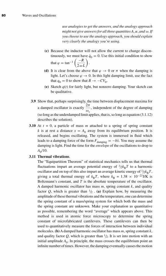
80 Waves and Oscillations
use analogies to get the answers, and the analogy approachmight not give answers for all three quantities A, α, and ω. Ifyou choose to use the analogy approach, you should explainvery clearly the analogy you’re using.
(c) Because the inductor will not allow the current to change discon-tinuously, we must have q0 = 0. Use this initial condition to show
that ϕ = tan−1
( −R
2 ω L
).
(d) It is clear from the above that ϕ → 0 or π when the damping islight. Let’s choose ϕ → 0. In this light damping limit, use the factthat q0 = 0 to show that B → −CV0.
(e) Sketch q(t) for fairly light, but nonzero damping. Your sketch canbe qualitative.
3.9 Show that, perhaps surprisingly, the time between displacement maxima for
a damped oscillator is exactly2π
ωv, independent of the degree of damping
(so long as the underdamped limit applies, that is, so long as equation (3.1.12)describes the solution).
3.10 At t = 0, a particle of mass m attached to a spring of spring constantk is at rest a distance x = A0 away from its equilibrium position. It isreleased, and begins oscillating. The system is immersed in fluid whichleads to a damping force of the form Fdamping = −bx. You may assume thedamping is light. Find the time for the envelope of the oscillations to drop toA0/10.
3.11 Thermal vibrations.The “Equipartition Theorem” of statistical mechanics tells us that thermalfluctuations impart an average potential energy of 1/2kBT to a harmonicoscillator and on top of this also impart an average kinetic energy of 1/2kBT ,giving a total thermal energy of kBT , where kB = 1.38 × 10⁻²³J/K isBoltzmann’s constant, and T is the absolute temperature of the oscillator.A damped harmonic oscillator has mass m, spring constant k, and qualityfactor Q, which is greater than 1/2 . (a) Explain how, by measuring theamplitude of these thermal vibrations and the temperature, one can determinethe spring constant of a mass/spring system for which both the mass andthe spring constant are unknown. Make your explanation as quantitativeas possible, remembering the word “average” which appears above. Thismethod is used in atomic force microscopy to determine the springconstant of microfabricated cantilevers. These cantilevers can then beused to quantitatively measure the forces of interaction between individualmolecules. (b) A damped harmonic oscillator has mass m, spring constant k,and quality factor Q, which is greater than 1/2. It is set into motion with aninitial amplitude A0. In principle, the mass crosses the equilibrium point aninfinite number of times. However, the damping eventually causes the motion

Chapter 3 ■ Damped Oscillations 81
to become smaller than random thermal motions. In terms of m, k, Q, A0,kB, and T about how long does this take?
3.12 For a damped harmonic oscillator, show that if Fdamp = −bxβ , then theenergy as measured on timescales longer than an oscillation period onlydecays exponentially if β = 1. Assume light damping. You may also assumethat Paverage = GPmax, where P is the dissipated power and G is a constant.Hint: If you assume that E decays exponentially, what differential equationinvolving Pav = E must be obeyed? Then, in this equation, write E in termsof the maximum kinetic energy. Finally, develop a second equation for Eusing Fdamp = −bxβ .
3.13 Damping by radiation. From classical electromagnetism, one can showthat the instantaneous power of electromagnetic radiation that is emitted
by a point charge q undergoing acceleration a is P = q2a2
6π ε0 c3, where c =
2.9979 × 10⁸ m/s is the speed of light and ε0 = 8.8542 × 10⁻¹² C2/Nm2 is thepermittivity of free space. Consider an electron that oscillates in harmonicmotion about a stable position with frequency f and amplitude A. It is heldclose to this position by forces from other charges. As usual, we assume thatthe net restoring force has a magnitude proportional to displacement awayfrom equilibrium. In this problem, you’ll show that the energy radiated awayprovides an effective viscous damping force.Assume that the energy radiatedby the electron in one cycle is much less than the energy in the oscillator, sothat over one cycle the motion is approximately sinusoidal. (a) Show that the
energy radiated in one cycle is Ecycle = 4π3e2A2f 3
3ε0c3. (b) Show that therefore
E
t∝ E, where E is the energy lost in one cycle and t equals one period.
(c) By comparison with equation (3.1.8), which appears in footnote 1, showthat the energy decays exponentially, just as with a viscous damping force,and find the time for the energy to decrease by a factor of e. (d) Show that
Q ∼= 3ε0mc3
e2f, where m is the mass of the electron.
3.14 Show that an overdamped oscillator can cross the equilibrium point onetime at most.
3.15 Show that x = Dte− γ2 t is a solution to equation (3.1.3) for the case of critical
damping. (In section 3. 5, we showed that x = Be− γ2 t is also a solution, so
the general solution is x = Be− γ2 t + Dte− γ
2 t .)3.16 For a given object moving through air or water, is the speed needed to
produce turbulence higher in air or water? Explain.3.17 Consider a round rock of radius r in a shallow stream. For about what velocity
of the stream should the flow around the rock become turbulent, accordingto the ideas discussed in this chapter? Is this velocity consistent with yourexperience?
3.18 You are designing a chemical processing plant, in which water from a pipeis used to fill a spherical reaction vessel that is 2 m in diameter. If there isturbulence inside the pipe, then the required pressure to force the water

82 Waves and Oscillations
through is significantly higher, so this is to be avoided. If the reactionvessel must be filled in less than 100 min, what is the minimum pipediameter?
3.19 Calibration of laser tweezers. As you may recall from an electricity andmagnetism course, matter is attracted to regions of high electric field. (Theatoms in the matter are polarized by the field, so that each atom forms adipole. The two ends of the dipole experience fields of different strength,leading to a net force.) You may also recall that light consists of rapidlyoscillating electric and magnetic fields. Combining these two ideas, we seethat there is an attractive force which draws matter into a region with themost intense light. For example, if you shine a laser beam into a drop of waterin which there are small plastic spheres suspended, the spheres are attractedinto the beam. This is called a “laser tweezers apparatus.” By moving thebeam around, you can drag one of these spheres wherever you like. Youcan also grab a living cell that is floating around in the water, and drag itaround without harming it. By combining two laser tweezers with a morepowerful laser that can cut through the cell wall (“laser scissors”), you canfuse two cells together. Going back to the plastic beads, you can attach onesort of molecule to the surface of a bead, allow it to bind to another sort ofmolecule on a different bead or on a solid surface, and measure the strengthof the binding by tugging with the laser tweezers. In order to perform thisexperiment, you must calibrate the strength of the force applied to the beadby the laser tweezers. Since the tweezers hold the bead in a position of stableequilibrium, the force applied to the bead by the laser can be approximatedby Hooke’s law, F = −kx, where x is the displacement of the center of thebead away from the center of the laser beam. One way to find the springconstant x is to flow water (or another fluid) past the bead at a known speedv0 and measure the resulting displacement x0 of the bead. Find an expressionfor k in terms of x0, v0, the viscosity μ of the surrounding fluid, the densityρ of the fluid, and the radius r of the bead, assuming the flow remainslaminar.
3.20 (a) Explain how our guess for the complex version of the solution of thedamped oscillator, (3.1.7): z = A0e−σ tei(ωvt+ϕ)could be written in the formz = Ceαt , where C and α are both complex. (b) Show that z = Ceαt is nota solution for the damped oscillator in the turbulent regime, where (3.6.3):
Fdrag = Cd
2Av2ρ.
3.21 Drag force for turbulent flow. (a) It is easier to think about drag forcesin a reference frame in which the object is stationary and the fluid medium(air, water, etc.) is moving past it. In laminar flow, the fluid moves aroundthe object with relatively little net disruption to its velocity. However, inturbulent flow, the velocity of the fluid is changed violently. Consider thevolume of fluid that will impinge on the object in a time t, as shown infigure 3.P.2. This has a length v t, and a cross-sectional area A equal to thatof the object.Assume that a fraction Cd/2 of the momentum of this volume offluid is transferred to the object. (Cd is called the “drag coefficient.”) Show

Chapter 3 ■ Damped Oscillations 83
Figure 3.P.2 In time t, all the air in the cylinder will hit the front of the spherical object.
that the resulting force on the object has a magnitude Fdrag = Cd
2Av2ρ,
where ρ is the density of the fluid. (b) For an airplane, Cd ≈ 0.03. Whatpower is required from the engines for an airplane with A = 15 m2 to flyat a speed of 150 kph near sea level, where the density of air is 1.2 kg/m3?(c) Repeat part (b) for a speed of 300 kph.

4 Driven Oscillations and Resonance
When you drive an oscillator at its resonant frequencyThen the amplitude of the oscillation will become huge.In the equation above, it becomes infinite,But in practice there will be some dampingThat prevents that.
You have known this since your childhood,This is how you swing on a swing.If you live in a snowy climate, you know(or at least should know) that a trickTo get your car out of a snow bank isTo rock it back and forth—
If you get the frequency right you will make the car oscillateWith a large amplitudeAnd dislodge it.
The electrical analogue is used to tune a radio.From “The Driven Oscillator” (not originally intended to be a poem)
by Professor B. Paul Padley, Rice University
4.1 Resonance
As we saw in chapter 3, the oscillations of a macroscopic oscillator decay over timebecause the energy leaks out into the surroundings. For an oscillation to be sustained,this energy loss must be balanced by the energy added to the oscillator. We see examplesof this all the time. A child on a swing uses her legs to pump the amplitude higher andhigher. The seat in a bus vibrates, because it is driven by the engine which is shakingin a regular way. A washing machine shakes, especially in the spin cycle; in this case,the energy is provided by the motor which spins the tub with the clothes in it. Thecurrent inside a radio receiver oscillates, driven by the radio waves broadcast by thetransmitter. The straps on your backpack, and your hair (if it’s long enough) swingback and forth as you walk, driven by the energy you put into moving your legs (whichalso moves your body up and down a little with each step).
84

Chapter 4 ■ Driven Oscillations and Resonance 85
The behavior of oscillators that are driven, including the above examples, isperhaps the single most important idea in all of physics. Essentially every area ofphysics has strong connections with driven oscillators, and many seemingly unrelatedphenomena can be understood qualitatively by analogy with driven oscillators.
You have probably noticed that if an oscillator is driven with a periodic force ofjust the right frequency, the motion of the oscillator becomes very large, much largerthan for other frequencies of drive force. For example, if you have an old car that rattlessometimes, you may have noticed that the rattle is worst when the engine is running ata particular speed—for lower speeds or for higher speeds the rattle is less noticeable.This phenomenon of a strong response at a certain frequency is called “resonance.” Itcan be annoying and even destructive, leading to failure of mechanical components,but it can also be used to almost magical effect in the design of ultrasensitive detectors,and in medical imaging, as shown in figure 4.1.1.
Following the approach of physics, we begin with the simplest possible drivenoscillator: a mass on a spring. However, by now you recognize that this can representa vast array of physical systems, including electronic circuits (which we’ll explorelater in this chapter). We will also assume to start that the energy injected into theoscillator comes from the simplest possible periodic source: a sinusoidal driving force.However, this is actually no restriction at all, since we will show that any periodicdriving force can be represented as a sum of sinusoids, and that the response of the linear
Figure 4.1.1 Magnetic resonance images of a human brain. (Image © KatrinaBrown/Dreamstime.com)
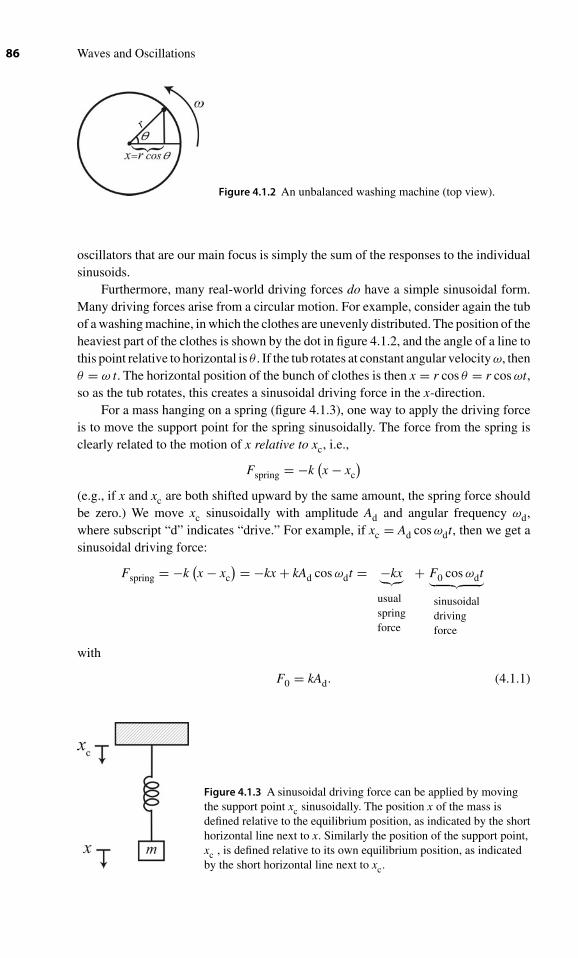
86 Waves and Oscillations
Figure 4.1.2 An unbalanced washing machine (top view).
oscillators that are our main focus is simply the sum of the responses to the individualsinusoids.
Furthermore, many real-world driving forces do have a simple sinusoidal form.Many driving forces arise from a circular motion. For example, consider again the tubof a washing machine, in which the clothes are unevenly distributed. The position of theheaviest part of the clothes is shown by the dot in figure 4.1.2, and the angle of a line tothis point relative to horizontal is θ . If the tub rotates at constant angular velocity ω, thenθ = ω t. The horizontal position of the bunch of clothes is then x = r cos θ = r cos ωt,so as the tub rotates, this creates a sinusoidal driving force in the x-direction.
For a mass hanging on a spring (figure 4.1.3), one way to apply the driving forceis to move the support point for the spring sinusoidally. The force from the spring isclearly related to the motion of x relative to xc, i.e.,
Fspring = −k(x − xc
)(e.g., if x and xc are both shifted upward by the same amount, the spring force shouldbe zero.) We move xc sinusoidally with amplitude Ad and angular frequency ωd,where subscript “d” indicates “drive.” For example, if xc = Ad cos ωdt, then we get asinusoidal driving force:
Fspring = −k(x − xc
) = −kx + kAd cos ωdt = −kx︸︷︷︸usualspringforce
+ F0 cos ωdt︸ ︷︷ ︸sinusoidaldrivingforce
with
F0 = kAd. (4.1.1)
Figure 4.1.3 A sinusoidal driving force can be applied by movingthe support point xc sinusoidally. The position x of the mass isdefined relative to the equilibrium position, as indicated by the shorthorizontal line next to x. Similarly the position of the support point,xc , is defined relative to its own equilibrium position, as indicatedby the short horizontal line next to xc.

Chapter 4 ■ Driven Oscillations and Resonance 87
Before starting our quantitative analysis, let’s qualitatively consider what toexpect. If the frequency of the drive is very low, then the mass should simply moveup and down together with the support point, that is, x = xc = Ad cos ωdt. On theother hand, if ωd is very high, then the sign of the drive force keeps changing at a highfrequency. So, the drive force doesn’t have much time to accelerate the mass before thesign of the drive force changes. So, for large ωd, we expect a small motion of the mass.Somewhere between low ωd and high ωd we expect to find a resonant response,that is, a special frequency of drive force for which the mass oscillates with largeamplitude.
The damped oscillator without a drive force is just a special case of the dampeddriven oscillator, with zero drive amplitude, that is, F0 = 0. Thus, the full solutionfor the oscillator with both driving and damping should include the possibility ofan oscillation at angular frequency ωv that decays away exponentially and has anamplitude and phase that depend on the initial position and velocity. However, fortimes well beyond t = 0, it is reasonable to expect that the effect of these initialconditions will decay away, and that we will see a “steady-state” oscillation in whichthe energy per cycle delivered to the system by the drive equals the energy per cyclethat leaks away from the system because of the damping. This “steady-state solution”is actually the one of most interest, since it persists indefinitely.
We consider a general sinusoidal drive force
Fdrive = F0 cos ωdt, (4.1.2)
which might be applied by a motion of the support point (equation (4.1.1), or mightbe applied in some other way.
To find the behavior of the system, x(t), we again follow our three-step procedure:
1. Write Newton’s second law for each object in the system:
mx = −kx − bx + F0 cos ωdt ⇔mx + bx + kx = F0 cos ωdt ⇔ (4.1.3a)
x + γ x + ω20 x = F0
mcos ωdt. (4.1.3b)
1b. Cast the DEQ into complex formFollowing the lead given by previous chapters, we write the simplest complexdifferential equation for which equation (4.1.3b) is the real part:
z + γ z + ω20 z = F0
meiωdt (4.1.4)
with x = Re(z).
2. Guess a solution, based on physical and mathematical intuitionDriven oscillators appear to show a regular motion, at least once the steady-statediscussed earlier has been achieved. It is not obvious whether the angular frequencyof this motion would be that of oscillation without damping or driving (ω0) or thatof oscillation with damping but no driving (ωv), or that of the drive (ωd) , or somecombination of these. So, for now, we write the angular frequency of the motion in

88 Waves and Oscillations
steady-state as ωs. To be as general as possible, we include a phase factor, and of coursean amplitude. Thus, our guess is
z?= Aei(ωs t−δ).
Here, the phase factor is written as −δ, rather than, for example, +ϕ. We do thisbecause it will turn out that δ as defined this way is always positive, though this is notyet obvious. The above guess can be rewritten
z?= Ae−iδeiωs t . (4.1.5)
3. Substitute the guess into the DEQ to see if it is a solution, and if there arerestrictions on the parameters
Your turn: Plug our guess (4.1.5) into (4.1.4) to show that
(−ω2s A + iγ ωsA + ω2
0A)e−iδeiωst ?= F0
meiωd t . (4.1.6)
We see that the left side oscillates at an angular frequency ωs, while the right sideoscillates at ωd. So, if they are to be equal, we must have ωs = ωd. In other words(assuming other aspects of our guess turn out to be correct):
In the steady-state, the oscillator moves with the same angular frequency asthe drive.
This is perhaps an unexpected result. In the steady-state, the system does not movewith its “natural” angular frequency ω0 or at ωv, but rather it moves at ωd.
So, our guess now becomes
z?= Ae−iδeiωd t , (4.1.7)
and is shown graphically in figure 4.1.4. But we haven’t yet shown that our guess reallyworks. Since ωs = ωd, equation (4.1.6) becomes
(−ω2dA + iγ ωdA + ω2
0A)e−iδeiωdt ?= F0
meiωd t .
⇒ (−ω2dA + iγ ωdA + ω2
0A)e−iδ ?= F0
m.
⇔ (ω20 − ω2
d)A + iγ ωd A?= F0
meiδ

Chapter 4 ■ Driven Oscillations and Resonance 89
Figure 4.1.4 Our guess represented in thecomplex plane. Note that, since the units of z and
F0 are different, the length of the two vectorscannot be compared.
For this equation to hold, the real part of the left side must equal the real part of theright side, and also the imaginary part of the left side must equal the imaginary part ofthe right side:
Real: (ω20 − ω2
d)A?= F0
mcos δ. (4.1.8)
Imaginary: γ ω dA?= F0
msin δ. (4.1.9)
To make these equations true, we will need particular values of A and δ. To isolate A,we square these two equations and add them, giving
A = A(ωd
) = F0/m√(ω2
0 − ω2d)2 + (γ ωd)2
, (4.1.10)
in which we emphasize that A is a function of ωd. To isolate δ, we instead divideequation (4.1.9) by (4.18), giving
tan δ(ωd
) = γ ωd
ω20 − ω2
d
, (4.1.11)
again emphasizing that δ is a function of ωd.1
So, our guess (4.1.7) is indeed a solution of the differential equation (4.1.4)! (Butonly if A and δ are as given above.) Of course,
x = Re (z) = A cos (ωdt − δ). (4.1.12)
We can see from equation (4.1.10) that the amplitude depends on the angular frequencyof the drive, ωd. It might appear from the equation that the maximum amplitude occurs
1. It is correct to write δ(ωd
) = tan−1 γ ωd
ω20 − ω2
d
, however recall that one must be careful with the
tan−1 function. For a negative argument, your calculator (or Mathematica or other equivalentprogram) returns a negative value for the tan−1. Since we want δ to be positive, we must add π
to such a result.

90 Waves and Oscillations
Figure 4.1.5 Amplitude and phase of adamped driven oscillator as a function of theangular frequency of the drive.
at ωd = ω0; this is almost right, but the actual maximum is at a slightly lower value2 ofωd. However, the difference is quite small, except for heavy damping, and is usuallyunimportant. (We shall discuss this in more detail in section 4.2.) This maximumamplitude is the resonance discussed earlier in this section.
We also see from equation (4.1.11) that the phase δ by which the oscillator’sresponse lags behind the drive force also depends on ωd. When ωd = ω0, equation(4.1.11) becomes tan δ → ∞, so that δ = π/2. The dependencies of A and δ on ωd areshown in figure 4.1.5.
We see from equation (4.1.10) that the response amplitude at high frequenciesapproaches zero, as anticipated in our initial qualitative discussion. In the oppositelimit, ωd → 0, equation (4.1.10) reduces to
A(ωd → 0
) = F0/m
ω20
= F0
k.
If the drive force is applied by moving the support point, then, using equation (4.1.1):F0 = kAd, this becomes
A(ωd → 0
) = Ad, (4.1.13)
which is also as we anticipated.
2. To see this, we rewrite equation (4.1.10):
A = F0/m√(ω2
0 − ω2d)2 + (γ ωd)2
= 1
ωd
F0/m√(ω2
0 − ω2d)2
ω2d
+ γ 2
︸ ︷︷ ︸peaks at ωd=ω0
.
The second part of this has a peak at exactly ωd = ω0. However, it is multiplied by the factor1/ωd, which increases as ωd decreases, shifting the peak to a slightly lower value of ωd.

Chapter 4 ■ Driven Oscillations and Resonance 91
4.2 Effects of damping
The shapes of the curves in figure 4.1.5 are profoundly important for applications ofresonance, both those applications in which we want to maximize resonance effects(such as in radio receivers) and applications in which we want to minimize them (suchas in building designs). These curves are strongly affected by the degree of damping,as we’ll explore in this section.
Often, it is revealing to re-express functions in terms of their dependence ondimensionless variables; this frequently reveals a universal behavior that was obscuredin the original form of the function. In our case, we will try re-expressing the steady-state amplitude A and the phase shift δ of the response relative to the drive force.In equations (4.1.10) and (4.1.11), these two functions are expressed in terms of theangular frequency of the drive, ωd and the factor γ ≡ b/m which characterizes thedamping. We will now re-express them in terms of ωd/ω0 and Q ≡ ω0/γ , both ofwhich are dimensionless.
Your turn: Starting from equation (4.1.10), A = F0/m√(ω2
0 − ω2d)2 + (γ ωd)2
, and using
γ = ω0/Q, show that A = F0/m
ω0 ωd
√(ω0
ωd− ωd
ω0
)2
+ 1
Q2
.
We can rewrite this result as A = F0
mω20
ω0/ωd√(ω0
ωd− ωd
ω0
)2
+ 1
Q2
. Since ω0 ≡√
k
m, this
becomes
A = F0
k
ω0/ωd√(ω0ωd
− ωdω0
)2 + 1Q2
. (4.2.1)
We can now see the universal behavior that we hoped would arise; the particular valuesof ωd and ω0 are not really central – what really matters is the ratio ωd/ω0.
If the drive force is applied by moving the support point, then equation (4.1.1):F0 = kAd, so that
A = Adω0/ωd√(
ω0ωd
− ωdω0
)2 + 1Q2
. (4.2.2)
This relation is graphed in figure 4.2.1. Several different curves are shown for differentvalues of Q. The most important effect of increasing the Q (i.e., lowering the damping)is to make the peak higher and sharper.
A more subtle effect is that the peak, which is always at an angular frequency closeto ω0, moves even closer to ω0 as Q increases. You can show in problem 4.8 that the

92 Waves and Oscillations
Figure 4.2.1 Dependence of steady state amplitude on ωd /ω0.
peak occurs at
ωd, peak = ω0
√1 − 1
2Q2. (4.2.3)
Recall from chapter 3 that Q = 2π corresponds to reasonably heavy damping. (Withouta driving force, the energy decays by a factor of 1/e per cycle, and the amplitude decaysby a factor of 1/
√e ∼= 0.61 per cycle.) Substituting Q = 2π into equation (4.2.3) gives
ωd,peak = 0.994 ω0. For light damping, ωd,peak is even closer to ω0, so for most purposesthe difference can be ignored.
For moderate to light damping, for which the peak amplitude occurs at ωd∼= ω0,
we can obtain a useful result for the height of the peak. Substituting ωd = ω0 intoequation (4.2.2) gives
A(ωd = ω0
) = QAd. (4.2.4)
In other words,
For light to moderate damping:(peak response amplitude) ∼= Q × (drive amplitude).
Since the low-frequency response amplitude is equal to the drive amplitude, we couldalso say that the peak response amplitude is Q times the low-frequency responseamplitude.
For ωd � ω0, the response becomes
A = Adω0/ωd√(
ω0ωd
− ωdω0
)2 + 1Q2
lim ωd�ω0−−−−−−→ Ad
(ω0
ωd
)2
, (4.2.5)
so that, at high frequencies, the response is universal, and does not even depend on thedegree of damping.

Chapter 4 ■ Driven Oscillations and Resonance 93
Figure 4.2.2 Phase shift δ of thesteady-state response.
Now, we will consider how the graph of the phase shift δ is affected by damping.Again, we begin by expressing δ in terms of the dimensionless quantities ωd/ω0 and Q.
Your turn: Starting from equation (4.1.11), tan δ = γ ωd
ω20 − ω2
d
, and using γ = ω0/Q,
show that
tan δ = 1/Qω0
ωd− ωd
ω0
. (4.2.6)
This relation is graphed in figure 4.2.2.3 At low ωd, the phase shift is zero, meaning(as we anticipated) that the oscillator moves in phase with the drive. At high ωd, thephase shift is 180◦; the oscillator is exactly out of phase with the drive. At ωd = ω0, thephase shift is exactly 90◦. The effect of increasing the Q (i.e., lowering the damping)is to sharpen the transition from δ = 0 at low drive frequency to δ = π at high-drivefrequency.
Connection to current research: Tapping Mode Atomic Force Microscopy
The Atomic Force Microscope (AFM), invented in 1986 by Gerd Binnig, Calvin Quate,and Christoph Gerber, images a sample by touching it very lightly with a sharp tipmounted on the end of a cantilever (figure 4.2.3). The upward force exerted on thetip by the sample causes a bend in the cantilever, so that this force can be measuredquantitatively. In the original mode of operation (“contact mode”), the tip is first loweredinto contact with the sample until a pre-set force is achieved (typically about 100nN). Then, the tip is moved laterally across the sample. As it moves, the force ismonitored, and the base of the cantilever is moved up or down as needed to keepthe force constant at the pre-set level. In this way, the microscope “feels” the shape
continued
3. We can rewrite equation (4.2.6) as δ = tan−1 1/Qω0
ωd− ωd
ω0
. Recall that, in this case if the argument
of the tan−1 function is negative, that is, if ωd > ω0, we must add π to the result given by acalculator or a program like Mathematica in order to get the correct value of δ. (See footnote 1after equation (4.1.11).)

of the surface, while only applying a light force. This works well for semiconductor andmetal samples, but the lateral motion of the tip is very destructive for the soft sampleswhich are of most interest in biology and in molecular electronics.
Figure 4.2.3 The cantilever for an atomic force microscope (top image) must have amoderately high Q, so that a small amplitude vibration applied at the base of thecantilever results in a vibration amplitude at the tip of about 100 nm. The length of thecantilever is 125 μm, about the same as the diameter of a human hair. Thepyramid-shaped tip located at the end of the cantilever (bottom image) must be verysharp to obtain high resolution images. (Image courtesy of Veeco Instruments Inc.)
In 1993, Zhong, Inniss, Kjoller, and Elings introduced the Tapping modeTM AFM. (Thetrademark belongs to Digital Instruments (now part of Veeco Corporation), which wasfounded by Virgil Elings and is the leading manufacturer of AFMs.) In this mode, the baseof the cantilever is vibrated vertically by means of a piezoelectric crystal. The frequencyof vibration is chosen to match the resonant frequency of the cantilever, so that the tipvibrates with an amplitude of about 100 nm. The vibration amplitude is measured, andthe base of the cantilever is slowly lowered toward the sample. When the tip beginsto tap the sample, this contact reduces the oscillation amplitude. The base is loweredfurther until the amplitude reaches a pre-set value. Then, as in contact mode, the baseof the cantilever is moved laterally across the sample. As it moves, the amplitude of thetip’s oscillation is monitored, and the base of the cantilever is moved up or down asneeded to keep the amplitude constant. Because the tip only touches the sample brieflyduring each cycle of oscillation, the lateral forces applied to soft features on the sampleare minimized, so that they can be imaged without damage.
The Q of the cantilever is typically about 100. Therefore, since A(ωd = ω0
) = QAd,the drive amplitude Ad applied by the piezoelectric crystal to the base of the cantileverneeds to be only about 1 nm in order to produce the desired tip vibration amplitudeA of 100 nm. This large ratio is essential, because if one had to vibrate the base by the full100 nm, the entire AFM would vibrate, dramatically degrading image quality.
94

Chapter 4 ■ Driven Oscillations and Resonance 95
4.3 Energy flow
Energy is perhaps the most fundamental idea in physics. In many situations, includingmany parts of quantum mechanics, finding the energy is the central problem. We willfind that, for damped driven oscillators, a careful consideration of the energy for thesteady-state behavior provides insights that can be very broadly applied.
The power (energy per time) supplied to the oscillator by the drive force is
Pdrive = Fdrivev.
In the steady-state, x = A cos (ωdt − δ), and so
v = x = −Aωd sin(ωdt − δ
) = Aωd sin(δ − ωdt
) = Aωd cos(δ − π/2 − ωdt
)= Aωd cos
(ωdt + π/2 − δ
)Therefore,
Pdrive = (F0 cos ωdt
)︸ ︷︷ ︸Fdrive
(Aωd cos
(ωdt + π/2 − δ
))︸ ︷︷ ︸v
. (4.3.1)
Concept test (answer4 below): For what value of ωd/ω0 are the oscillations of Fdrivein phase with the oscillations in v? Hint: review figure 4.2.2.
Since, for the value you just found, the oscillations are always in phase, Pdrive isalways positive, that is, the drive force always supplies power to the oscillator. For anyother value of ωd/ω0, the oscillations of Fdrive are not in phase with the oscillations in v;therefore, for some parts of the cycle Pdrive is positive (the drive force supplies power tothe oscillator), and for some parts of the cycle Pdrive is negative (the oscillator suppliespower to the entity providing the drive force). An example is shown in figure 4.3.1a.We can define Pdrive, av to be the power supplied by the drive averaged over a cycle.For the example shown in figure 4.3.1a, Pdrive is positive for most of the cycle, soPdrive, av > 0.
As ωd → 0, δ → 0, so that Fdrive and v are out of phase by π /2. For this condition,the net energy flowing from the drive to the oscillator is zero (i.e., Pdrive, av = 0), assuggested in figure 4.3.1b. (You can show rigorously that the net energy flow is zeroin problem 4.11.) As ωd → ∞, δ → π , so that Fdrive and v are out of phase by π /2 inthe other direction; again the net flow of energy from the drive over a cycle is zero.Putting all this together, we expect that the graph of Pdrive, av as a function of ωd/ω0must start at zero, reach a peak (probably at ωd/ω0 = 1), and then go back to zero.
Let’s examine this quantitatively. The average power, Pdrive, av, can be computedusing the average value theorem from calculus:
Pdrive,av = 1
T
T∫0
Pdrivedt,
4. For the oscillations to be in phase, we need δ = π /2, which occurs when ωd/ω0 = 1.

96 Waves and Oscillations
Figure 4.3.1 a: Fdrive and v for the case δ = 45◦. In the shaded regions, the two have oppositesign, so Pdrive is negative, meaning that the oscillator supplies power to the drive. In the otherregions, Fdrive and v have the same sign, so Pdrive is positive, and the drive supplies power tothe oscillator. (Since Fdrive and v have different units, the vertical scales cannot be compared.)b: Fdrive and v for ωd → 0; in this limit δ → 0, so Fdrive and v are out of phase by π /2. In theshaded regions, the two have opposite sign, so Pdrive is negative, meaning that the oscillatorsupplies power to the drive. In the other regions, Fdrive and v have the same sign, so Pdrive ispositive, and the drive supplies power to the oscillator. (The velocity scale for this plot isgreatly magnified compared to part a; for small ωd , the velocity is also small.)
where T is the period of the steady-state motion. Plugging in our expression fromequation (4.3.1), we get
Pdrive = 1
T
T∫0
(F0 cos ωdt
)Aωd cos
(ωdt + π/2 − δ
)dt
= F0Aωd
T
T∫0
cos ωdt cos(ωdt + π/2 − δ
)dt.
This integral can be evaluated using Mathematica, or a similar symbolic algebraprogram or calculator; it can also be done “by hand” as shown in the footnote.5 Bearing
5. First, we re-express the second term in the integral: cos(ωdt + π/2 − δ
) = cos(δ −
π/2 − ωdt) = sin
(δ − ωdt
). Therefore, Pdrive = F0Aωd
T
T∫0
cos ωdt sin(δ − ωdt
)dt.
Next, we use sin (A + B) = sin A cos B + cos A sin B, so that Pdrive =

Chapter 4 ■ Driven Oscillations and Resonance 97
Figure 4.3.2 Geometric representation of equation (4.2.6).
in mind that T = 2π/ωd, the result is
Pdrive, av = F0Aωd
2sin δ. (4.3.2)
To evaluate sin δ, we can represent equation (4.2.6) geometrically, as shown infigure 4.3.2. From this, we see that
sin δ = 1/Q√(ω0ωd
− ωdω0
)2 + 1Q2
.
Your turn: Substitute the above, and also equation (4.2.1): A = F0
k
ω0/ωd√(ω0
ωd− ωd
ω0
)2
+ 1
Q2
into equation (4.3.2), and show that the result is
Pdrive, av = F20ω0
2kQ
1(ω0
ωd− ωd
ω0
)2
+ 1
Q2
. (4.3.3)
F0Aωd
T
[sin δ
T∫0
cos ωdt cos(−ωdt
)dt + cos δ
T∫0
cos ωdt sin(−ωdt
)dt
]. This simplifies
to Pdrive = F0Aωd
T
[sin δ
T∫0
cos2 ωdt dt − cos δT∫0
cos ωdt sin ωdt dt
]. These are both
standard integrals which can be looked up in a table. The first one is especially important:T∫0
cos2 ωdt dt =[
t
2+ 1
4ωdsin 2ωdt
]T
0
. Since T = 2π/ωd, the second term evaluates to
zero at both limits, so that the integral is just T /2. Since we integrated over a wholeperiod, we can see that the average value of a squared sinusoid over one period is 1/2.The second integral can also be looked up in a table (or you can integrate it by parts):T∫0
cos ωdt sin ωdt dt =[
1
2ωdsin2 ωdt
]T
0
. Since T = 2π/ωd, this evaluates to zero at both limits.
Putting this all together gives Pdrive = F0Aωd
T
T
2sin δ = F0Aωd
2sin δ.

98 Waves and Oscillations
This relation is plotted in figure 4.3.3a. Inspection of the equation shows that the peakis at exactly ωd/ω0 = 1. As for the graph of A versus ωd (figure 4.2.1), larger Q (lessdamping) leads to a higher and sharper peak.
The width of the peak is quite important for a variety of applications. One commonway to define the width is the “full width at half maximum,” or FWHM, which is thewidth at half of the peak height, as shown in figure 4.3.3b. Let us calculate the FWHMexactly. Referring to equation (4.3.3), we see that the values of ωd corresponding tohalf the maximum height are determined by
(ω0
ω±− ω±
ω0
)2
= 1
Q2, (4.3.4)
where ω± is either ω+ or ω−. First, we consider ω−. Since ω0 > ω−, equation (4.3.4)gives
ω20 − ω2
− = ω0 ω−Q
⇔ ω2− + ω0 ω−
Q− ω2
0 = 0 ⇒ ω− =−ω0
Q ±√
ω20
Q2 + 4ω20
2.
Since ω− must be greater than 0, we choose the positive square root, giving
ω− = − ω0
2Q+ 1
2
√ω2
0
Q2+ 4ω2
0.
Figure 4.3.3 a: Power delivered by drive force to oscillator (averaged over a cycle) as afunction of ωd. This is called the power resonance curve. b: Definition of FWHM.
Chapter 4 ■ Driven Oscillations and Resonance 99
Next, we consider ω+. Since ω+ > ω0, equation (4.3.4) gives
ω2+ − ω20 = ω0 ω+
Q ⇔ ω2+ − ω0 ω+Q − ω2
0 = 0
⇒ ω+ =ω0
Q±
√ω2
0
Q2+ 4ω2
0
2.
Since ω+ must be greater than 0, we choose the positive square root, giving
ω+ = ω0
2Q+ 1
2
√ω2
0
Q2+ 4ω4
0 .
The FWHM is given by ω+ − ω−, so that
FWHM = ω0
Q= γ. (4.3.5)
Full Width at Half Maximum for the graph of Pdrive, av versus ωd.
This important equation tells us that systems with more damping have a broader powerresonance peak. This is a very universal behavior, which is observed even for systemswith turbulence or frictional damping.
4.4 Linear differential equations, the superposition principle fordriven systems, and the response to multiple drive forces
What happens if we apply a nonsinusoidal drive force, or if we apply two or threedifferent sinusoids at different frequencies and amplitudes? We will show in chapter 8that any function can be represented as a sum of sinusoids. Therefore, if we can figureout how a damped driven oscillator responds to multiple sinusoidal drives, it will berelatively easy, after understanding the contents of chapter 8, to determine the responseto any driving force.
We will make use of an important property of the differential equation governinga damped driven oscillator:
mx = −kx − bx + F0 cos ωdt ⇒ x + γ x + ω20 x = F0
mcos ωdt.
This differential equation is linear, meaning that it has no terms proportional to x2, orto x2, or to xx, etc. That means, for example, that if we multiply x by two, then theentire left side of the above equation becomes twice as big. (This would not be true,for example, if the left side were x2.) It also means, as we’re about to show, that we cansimply add the steady-state solutions for each of the individual driving forces to get thesteady-state solution for the combined driving force. The term on the right side, whichdoes not depend on x, and which comes from the drive (also called the excitation) iscalled the “source term.”
100 Waves and Oscillations
We’ll be able to see the pattern for the response to any number of sinusoidal drivingforces by considering the case of just two:
Fdrive = F1 cos ω1t + F2 cos ω2t.
To find the behavior of the system, x(t), we begin to follow our three-step procedure,though this time it will be surprisingly easy so that we don’t have to go through thewhole process.
1. Write Newton’s second law for each object in the system:
mx = −kx − bx + F1 cos ω1t + F2 cos ω2t ⇒
x + γ x + ω20 x = F1
mcos ω1t + F2
mcos ω2t. (4.4.1)
If the drive force is simply Fdrive = F1 cos ω1t, then we know that the steady-state response is x1 (t) = A1 cos
(ω1t − δ1
), where A1 and δ1 are as given by
equations (4.1.10) and (4.1.11), simply replacing F0 by F1 and ωd by ω1:
A1 = F1/m√(ω2
0 − ω21)2 + (γ ω1)2
and tan δ1 = γ ω1
ω20 − ω2
1
. (4.4.2)
We know that, for this simple drive force, we have
x1 + γ x1 + ω20 x1 = F1
mcos ω1t. (4.4.3)
Similarly, if the drive force is simply Fdrive = F2 cos ω2t, then the steady-state responseis x2 (t) = A2 cos
(ω2t − δ2
), where A2 and δ2 are defined analogously to equation
(4.4.2). For this simple drive force, we have
x2 + γ x2 + ω20 x2 = F2
mcos ω2t. (4.4.4)
Adding equation (4.4.4) to (4.4.3) gives
x1 + γ x1 + ω20 x1 + x2 + γ x2 + ω2
0 x2 = F1
mcos ω1t + F2
mcos ω2t
⇔ (x1 + x2
) + γ(x1 + x2
) + ω20
(x1 + x2
) = F1
mcos ω1t + F2
mcos ω2t
.
⇒ xtot + γ xtot + ω20 xtot = F1
mcos ω1t + F2
mcos ω2t, (4.4.5)
where xtot (t) ≡ x1 (t) + x2 (t) = A1 cos(ω1t − δ1
) + A2 cos(ω2t − δ2
). We see that
equation (4.4.5) is the same as equation (4.4.1). Therefore,
The steady-state response of a damped driven oscillator to two sinusoidal drive forces issimply the sum of the steady state responses to each force by itself.
It is easy to see that if we have seven sinusoidal drive forces, or seventy timesseven sinusoidal drive forces, then the steady-state response is simply the sum of theindividual responses.

Chapter 4 ■ Driven Oscillations and Resonance 101
Figure 4.4.1 Waves on a water surface are governed by a linear differential equation (if theyare small in amplitude), and so different wave patterns simply add, as shown here. Image ©Andrew Davidhazy, Rochester Institute of Technology.
This principle, that the total solution is simply the sum of the individual solutions,is called the “superposition principle” and only works for linear differential equations.Luckily, many important differential equations in physics are linear, so we can use thisprinciple in many contexts. (See, e.g., figure 4.4.1.)
The superposition principle for driven systems: For a system governed by a linear
differential equation, the total response to multiple excitations is the sum of the
response for each excitation applied individually.
4.5 Transients
Recall that the goal of section 4.1 was to find the steady-state behavior, that is, thebehavior after any effects of initial conditions have decayed away because of thedamping. Indeed, examination of the solution we found there shows that there are noconstants that can be adjusted to take into account variations of the initial position orvelocity:
(4.1.12): x = A cos(ωdt − δ), where
(4.1.10): A = F0/m√(ω2
0 − ω2d)2 + (γ ωd)2
and
(4.1.11): tan δ(ωd
) = γ ωd
ω20 − ω2
d
.
In almost every case, the steady-state behavior is the only thing of interest. But, thereare a few circumstances in which the initial behavior, which does depend on x0 andx0, is important. (See, e.g., figure 4.5.1.)
The solution x = A cos (ωdt − δ) is a solution to our differential equation,
(4.1.3b): x + γ x + ω20 x = F0
mcos ωdt,

102 Waves and Oscillations
Figure 4.5.1 The overall impression made by a musical instrument is strongly influenced bythe “attack,” that is, the way a note starts up from silence. This is an example of transientbehavior, and the transition to steady state. The graph shows a simulation of the attack for aflute; the larger amplitude waveform shows air density variations inside the flute, while thesmaller waveform shows the variation outside near the mouthpiece. Top image © GalinaBarskaya | Dreamstime.com. Bottom image © and courtesy of Dr. Helmut Kuehnelt.
but it cannot be the general solution; we know the general solution must include twoadjustable constants, which can be changed to reflect the effects of x0 and x0. So, wecan anticipate that the general solution must be the sum of x = A cos (ωdt − δ) withsomething that decays away over time and that depends on x0 and x0. It is actuallyquite easy to find the general solution, using the work we have already done.
Consider the special case F0 = 0; this is one of the cases that must be describedby the general solution. The differential equation for this special case is
x + γ x + ω20 x = 0, (4.5.1)
which describes the damped oscillator without driving. We already found the generalsolution for this case in section 3.1:
(3.1.12): x = A0 e− γ2 t cos
(ωvt + ϕ
),

Chapter 4 ■ Driven Oscillations and Resonance 103
where A0 and ϕ are determined by the initial conditions x0 and x0. Since this is thesolution to equation (4.1.3b): x + γ x + ω2
0 x = F0m cos ωdt for the special case of
F0 → 0, it is reasonable to guess that the general solution to equation (4.1.3b) is thesum of this and equation (4.1.12):
xG?= A0e− γ
2 t cos(ωvt + ϕ
)︸ ︷︷ ︸transient behavior
+ A cos(ωdt − δ
)︸ ︷︷ ︸steady-state behavior
. (4.5.2)
We can see that this works for the special case F0 = 0 (since, according to equation(4.1.10), A = 0 for this case), and also that it works for the steady-state, since the firstterm decays away over time. It has two adjustable constants A0 and ϕ, as we knowthe general solution must. Is it in fact a solution of our differential equation (4.1.3b)above?
To facilitate our checking, we introduce some nomenclature: equation (4.5.1) iscalled the “homogeneous” version of equation (4.1.3b), because it has zero on the rightside. So, equation (3.1.12) is the general solution to the homogeneous version of thedifferential equation, and we’ll call it xH:
xH = A0e− γ2 t cos
(ωvt + ϕ
). (4.5.3)
The steady-state solution (4.1.12) is a “particular solution” to the full version (theinhomogeneous version) of the differential equation (4.1.3b), so we call it xP:
xP = A cos(ωdt − δ
). (4.5.4)
Now, we are ready to check whether our guess xG?= xH + xP is a solution to
equation (4.1.3b):
xG + γ xG + ω20 xG
?= F0
mcos ωdt,
⇔ d2
dt2
(xH + xP
) + γd
dt
(xH + xP
) + ω20
(xH + xP
) ?= F0
mcos ωdt
⇔(
xH + γ xH + ω20 xH
)+
(xP + γ xP + ω2
0 xP
)?= F0
mcos ωdt.
We know that xH is a solution of equation (4.5.1): x + γ x + ω20 x = 0, so the first term
in parentheses equals zero. We know that xP is a solution of equation (4.1.3b), so thesecond term in parentheses equals F0
m cos ωdt. Thus, the equation is indeed satisfied,and the general solution for the damped driven harmonic oscillator is
xG = A0e− γ2 t cos
(ωvt + ϕ
)︸ ︷︷ ︸transient behavior
+ A cos(ωdt − δ
)︸ ︷︷ ︸steady- state behavior
, (4.5.5)
where A0 and ϕ are determined by the initial conditions x0 and x0. A typical exampleis shown in figure 4.5.2.

104 Waves and Oscillations
Figure 4.5.2 The full solution (bottom trace)for the damped driven harmonic oscillator isthe sum of the general solution for thedamped oscillator xH (top gray trace) and thesteady-state solution xP (top black trace).
4.6 Electrical resonance
In section 3.2, we discussed the RLC electrical oscillator, shown in the top part offigure 4.6.1. We applied Kirchhoff’s loop rule to obtain
VL + VR + VC = 0 ⇒Lq + Rq + q
C= 0.
To add driving, we open the loop and apply a drive voltage, as shown in the bottompart of figure 4.6.1. Now, instead of the voltage changes around the loop summing tozero, they must sum to the applied voltage, so that
Lq + Rq + q
C= V0 cos ωdt. (4.6.1)
This is isomorphic to the differential equation for the damped driven mass/springsystem, (4.1.3a):
mx + bx + kx = F0 cos ωdt.
So, the full isomorphism is as shown in table 4.6.1.
Concept test (answer below6): In terms of R, L, and C , what is Q for the circuit shownin the bottom part of figure 4.6.1?
6. Q = ω0/γ . For the mass/spring, ω0 = √k/m, which translates for the electrical oscillator
into ω0 = √1/LC. For the mechanical oscillator, γ = b/m, which translates into γ = R/L.
Combining gives Q =√
1
LC
L
R= 1
R
√L
C.
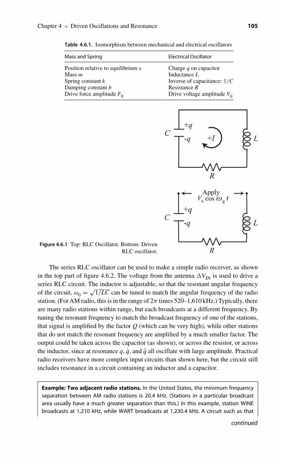
Chapter 4 ■ Driven Oscillations and Resonance 105
Table 4.6.1. Isomorphism between mechanical and electrical oscillators
Mass and Spring Electrical Oscillator
Position relative to equilibrium x Charge q on capacitorMass m Inductance LSpring constant k Inverse of capacitance: 1/CDamping constant b Resistance RDrive force amplitude F0 Drive voltage amplitude V0
Figure 4.6.1 Top: RLC Oscillator. Bottom: DrivenRLC oscillator.
The series RLC oscillator can be used to make a simple radio receiver, as shownin the top part of figure 4.6.2. The voltage from the antenna VIN is used to drive aseries RLC circuit. The inductor is adjustable, so that the resonant angular frequencyof the circuit, ω0 = √
1/LC can be tuned to match the angular frequency of the radiostation. (ForAM radio, this is in the range of 2π times 520–1,610 kHz.) Typically, thereare many radio stations within range, but each broadcasts at a different frequency. Bytuning the resonant frequency to match the broadcast frequency of one of the stations,that signal is amplified by the factor Q (which can be very high), while other stationsthat do not match the resonant frequency are amplified by a much smaller factor. Theoutput could be taken across the capacitor (as shown), or across the resistor, or acrossthe inductor, since at resonance q, q, and q all oscillate with large amplitude. Practicalradio receivers have more complex input circuits than shown here, but the circuit stillincludes resonance in a circuit containing an inductor and a capacitor.
Example: Two adjacent radio stations. In the United States, the minimum frequencyseparation between AM radio stations is 20.4 kHz. (Stations in a particular broadcastarea usually have a much greater separation than this.) In this example, station WINEbroadcasts at 1,210 kHz, while WART broadcasts at 1,230.4 kHz. A circuit such as that
continued

Figure 4.6.2 Top: The front end of a simple radio receiver. The arrow on the inductor indicatesthat it has a variable inductance, allowing the resonance frequency of the LRC circuit to betuned to match the frequency of the desired radio station. Bottom: Radio broadcast towers areoften grouped together to take advantage of a good site. As we’ll see in chapter 9, thedifferential equation governing radio waves is linear, so the different signals simply add. Aresonant RLC circuit inside a receiver, tuned to the broadcast frequency of one of the stations,is used as part of the circuitry that selects one of the stations out of the many signals that arereceived. Image © Tose | Dreamstime.com.
shown in figure 4.6.2 is tuned to a resonant angular frequency of 2π · 1, 210 kHz. What isthe required Q if the power dissipated in the resistor due to the WART signal is to be halfthe power dissipated due to the WINE signal?
Solution: Because the circuit is tuned to the angular frequency of WINE, the centerangular frequency ω0 for the power resonance curve (see figure 4.3.3b) is that of WINE. Insteady state, the power dissipated is equal to the power provided by the drive. We needthe power dissipated by the WART signal to be half that dissipated by the WINE signal,meaning that the angular frequency of the WART signal should correspond to the halfmaximum point of the power resonance curve (marked ω+ in figure 4.3.3b). We knowfrom equation (4.3.5) that the full width at half maximum of the power resonance curve
is given by FWHM = ω0Q ⇔ Q = ω0
FWHM. We need half the FWHM to equal the difference
in angular frequency between WART and WINE:
FWHM2
= 2π × 20.4 kHz ⇔ FWHM = 4π × 20.4 kHz.
Recall that the resonant angular frequency of the circuit is given as ω0 = 2π ×1, 210 kHz.
So, we have Q = 2π × 1, 210 kHz4π × 20.4 kHz
= 29.7.
106

Chapter 4 ■ Driven Oscillations and Resonance 107
4.7 Other examples of resonance: MRI and other spectroscopies
Of course, every oscillator described in chapter 2 can exhibit resonance when driven.However, the idea of resonance, meaning a strong response of system at or near aparticular excitation frequency, appears in many other situations as well. In this section,we briefly explore two of these.
Semiclassical description of Magnetic Resonance Imaging (MRI). MRI isbased on the phenomenon of Nuclear Magnetic Resonance (NMR). The nuclei inthe atoms of the body are comprised of protons and neutrons. We will treat these usinga “semiclassical” description, meaning a hybrid of classical and quantum mechanicalideas. Although this description does not capture the full quantum mechanical truth,it does allow us to get a feel of what is going on, and it also allows fully quantitativepredictions for the results of experiments. In this description, we visualize the protonsas tiny spinning spheres. Because the protons carry charge, the spin creates a circulatingelectrical current. As you’ll recall from a course in electricity and magnetism, acirculating current creates a magnetic field. Therefore, as shown in figure 4.7.1, eachproton acts as a tiny bar magnet, albeit one with some unusual properties. Becausethe magnetic moment μ of the proton is due to the spin, it is proportional to the spinangular momentum J:
μ = γ J, (4.7.1)
where the proportionality constant γ is called the gyromagnetic ratio, and dependson the type of the nucleus. (In quantum mechanics, one often uses J to represent theangular momentum, rather than L.)
Now, we apply an external magnetic field, Bapplied. (In an MRI instrument, this isusually produced by current flowing through a large coil that surrounds the patient.)From introductory electricity and magnetism, this field creates a torque on any magnetic
Figure 4.7.1 Semiclassical model for the magnetic moment of a proton. The proton is picturedas a spinning sphere, which creates a magnetic field similar to that of a bar magnet. Thus, theproton has a magnetic moment μ. An applied external magnetic field exerts a torque τ on thismagnetic moment; the torque points into the page.

108 Waves and Oscillations
moment (including that of the nucleus):
τ = μ × Bapplied. (4.7.2)
The torque tends to align the magnetic moment along the direction of Bapplied.However, quantum mechanics tells us that, surprisingly, μ doesn’t actually fully
line up with Bapplied; instead, there is a well-defined angle θ between these two vectors.One of the most important types of nuclei used for MRI is hydrogen; this is abundantin virtually all the molecules that make up the body. For hydrogen, θ = 54.7◦.
Because μ is not fully lined up with Bapplied, we have a body with a significantangular momentum (the nucleus) that experiences a torque. As you may recall from ademonstration in an earlier course involving a weighted bicycle wheel or a gyroscope,surprising things happen in this circumstance. Let’s take the example of a child’s topthat is tilted, as shown in figure 4.7.2a. In the side view, we can calculate the torquedue to gravity around the point at the bottom of the top. The weight can be taken asapplied at the center of mass, and therefore creates a torque
τ = r × F.
Using the right-hand rule for the cross-product, this torque points out of the page.Another way to find the direction of the torque: If the top weren’t spinning, it wouldfall down, rotating counterclockwise about the point at the bottom. Curling the fingersof your right hand in the direction of rotation that the torque is “trying” to produce, yourthumb points out of the page, in the direction of τ . However, because the top alreadyhas angular momentum, this torque does not cause it simply to fall over. Recall that
τ = dL/dt ⇔ dL = τdt,
where L is the angular momentum of the top. Therefore, the change in the angularmomentum is in the direction of τ , which is perpendicular to L. So, the length of Ldoesn’t change, but its direction does: in time dt, the the tip of the L vector moves aninfinitesimal amount out of the page. Since L is along the axis of rotation of the top,this means that the axis of rotation moves as well. This doesn’t fundamentally changethe situation, so the direction of the torque τ changes by an infinitesimal amount aswell, and is still perpendicular to L. Thus, the tip of L will trace out a circle with a“radius” (in units of angular momentum) equal to the x-component of L, as shown infigure 4.7.2c:
“radius” of circle = Lx = L sin θ.
This motion of the axis of rotation is called “precession.” If there were no friction toslow down the spinning of the top, it would continue to precess in this way withoutever falling down.
The “speed” (in units of angular momentum per time) of the tip of L as it movesalong this circle is τ = dL/dt. Therefore, the time it takes for one full circle is
time = “distance”
“speed”= 2π “radius”
τ= 2πL sin θ
τ.
The frequency of the precession is the inverse of this time:
f = τ
2πL sin θ. (4.7.3)

Chapter 4 ■ Driven Oscillations and Resonance 109
Figure 4.7.2 a and b: A child’s top that is tilted experiences a torque which is perpendicular tothe angular momentum L. c: The torque causes L to precess around a circle. d: We define areference frame that rotates at the precession rate. In MRI, a pulse of RF radiation is applied,with the magnetic field along the x-axis (in the nonrotating frame).
Applying these ideas to the nucleus with the applied external magnetic field, the tip ofμ precesses in the same way as does the axis of rotation of the top, moving in a circlearound the direction of Bapplied. As the tip moves in this circle, the vector μ sweepsthrough a cone, as shown in figure 4.7.2d.7 Combining equations (4.7.2) and (4.7.3),and using J to denote the magnitude of the spin angular momentum (rather than L),we find that the precession frequency is
f = τ
2πJ sin θ= μBapplied sin θ
2πJ sin θ= μBapplied
2πJ.
7. Recall that this is a semi-classical treatment. In a fully quantum mechanical treatment, thedirection of μ cannot be fully determined, due to an uncertainty principle similar to thosediscussed in section 1.12. We discussed there how the momentum and the position of a particlecannot both be precisely defined simultaneously. Similarly, it turns out that the components ofμ along the x-, y-, and z-axes cannot all be precisely defined simultaneously. In our example, thelength of μ is precisely defined, and the component along the direction of Bapplied is preciselydefined, but the components in the other directions are completely undefined. We sometimes saythat μ is “delocalized” around the cone. Careful consideration of these effects produce the sameresults as our semi-classical argument.

110 Waves and Oscillations
Substituting for μ from equation (4.7.1) gives
f = γ JBapplied
2πJ⇒ .
fLarmor = γ
2πBapplied, (4.7.4)
where this precession frequency is named the “Larmor frequency” after Joseph Larmor,an Irish physicist who occupied the same professorship at Cambridge University asdid Isaac Newton. Because there is no dissipation in the system, the magnetic momentμ of the nucleus precesses around the direction of Bapplied forever, unless somethingelse happens.
For MRI, the “something else” happens when we apply a pulse of radio frequency(RF) electromagnetic radiation, with a frequency equal to fLarmor. Let us define thez-axis to lie along Bapplied. The MRI machine is arranged so that this RF radiationtravels in the z-direction.As you may recall from a course in electricity and magnetism,electromagnetic radiation consists of waves of perpendicular electric and magneticfields, both of which are perpendicular to the direction of travel. (We shall explorethese in more detail in chapter 9.) Therefore, the magnetic field of the RF radiation,Brad could oscillate along any direction in the x–y plane. For convenience, we take it tooscillate along the x-axis. This oscillation at frequency fLarmor and angular frequencyωLarmor = 2π fLarmor can be considered to be the sum of two counter-rotating magneticfield vectors, each of which has angular velocity ωLarmor, as shown in figure 4.7.3a.We call the clockwise-rotating vector Brad, cl; it rotates at the same rate and in the samedirection as does the precessing magnetic moment μ of the nucleus.
We now consider what things look like in a rotating reference frame x’, y’, z’ thatrotates clockwise along with μ, with z’ parallel to z. Since Brad, cl rotates at the samerate as μ, it points in a constant direction in this frame. Let us define this direction tobe x’, as shown in figure 4.7.3b.
Figure 4.7.3 a: An oscillating magnetic field alongthe x-axis equals the sum of two counter-rotatingmagnetic fields. If the angular frequency of the RFpulse equals the Larmor frequency, then Brad, clrotates at the precession rate, and so is stationary inthe rotating reference frame. b: Taking Brad, cl to liealong x′, it causes a precession of the magnetizationaround the x′ axis. If the pulse length is chosensuitably, the magnetization can be rotated by 90◦.
Chapter 4 ■ Driven Oscillations and Resonance 111
At this point, we take a step back from thinking about the individual nuclei, andinstead consider the net magnetization M of a small region of the patient inside theMRI machine. This magnetization is due to the average of the magnetic moments ofthe nuclei, and so points along z. We have seen that a magnetic moment precessesabout the direction of an applied magnetic field. Because the magnetization is dueto the average of many magnetic moments, it also precesses about any applied field.Before the application of Brad, M is parallel to Bapplied, and so is stationary. WhenBrad is applied, Brad, cl points in a constant direction in the rotating reference frame,and M precesses about it. (In the rotating reference frame, Brad, ccl rotates at angularfrequency 2ωLarmor, and so has no average effect.)
We can control how far M precesses by the duration of the RF radiation pulse.Because M results from the average of all the individual magnetic moments of theatoms, the precession of M around the magnetic field due to the RF pulse, as seen inthe rotating frame, is governed by the same physics leading to equation (4.7.4), so thatthe angular rate of rotation is ω = γ Brad, cl. In the simplest version of MRI, the pulselength is chosen so that M precesses by 90◦ in the rotating reference frame, so thatafter this precession it lies along the y’ axis, as shown in figure 4.7.3b. A pulse of thislength is called a 90◦ or π /2 pulse.
In the stationary reference frame, the y’axis rotates clockwise at angular frequencyωLarmor around the z-axis. Therefore, after a 90◦ pulse has been applied so that M liesalong the y’ axis, it also rotates clockwise at ωLarmor. This rotating magnetizationbroadcasts electromagnetic radiation, which can be detected by the MRI machine.This whole mechanism only works when the frequency of the radiation in the RF pulsematches fLarmor. Any other frequency of radiation would have a magnetic field that isnot stationary in the rotating frame, and so produces no average effect.
Several different techniques are used to get contrast between different body tissuesin MRI. The simplest is associated with the effect of nearby electrons on the Bappliedthat is felt by a particular nucleus. The externally applied magnetic field affects themotion of these electrons, and since moving electrons create a magnetic field, the totalmagnetic field experienced by the nucleus depends on the local density of electrons.Nuclei in different types of molecules, and in different parts of the same molecule, aresurrounded by different densities of electrons. From equation (4.7.4), fLarmor dependson the total Bapplied. Therefore, these nuclei respond to different frequencies for theRF radiation pulse, giving contrast.
The rotation of M away from Bapplied increases the potential energy of the system;this energy comes from the RF radiation pulse. We have seen that this transfer ofenergy from the radiation to the nucleus can only occur if the radiation has the correctfrequency, fLarmor.
There is a rather different way of understanding the transfer of energy fromthe radiation to the nucleus, which generalizes to many other situations, but is lessconnected to classical physics. Even in a rather strong applied magnetic field, the effectof the field on the nuclei is small compared to that of random thermal fluctuations. Thisfact does not affect the above arguments, which are based on the average magnetization.Let us consider again the particular case of hydrogen nuclei. If one measures μz (thecomponent of μ in the direction of Bapplied), then surprisingly one finds that the resultis always one of two possibilities. Slightly more than half the time, one gets the result

112 Waves and Oscillations
for μz that one would expect from figure 4.7.1, with θ = 54.7◦; this is called “spin up,”because the direction of the nuclear spin axis is as close to the direction of Bappliedas it ever gets. Slightly less than half the time one gets the result, one would expectfor θ = 180◦ − 54.7◦ = 125.3◦; this is called “spin down.” This surprising findingthat only these two results are measured and nothing in between, is a purely quantummechanical effect with no classical analog. You might ask, “Weren’t we just talkingabout the magnetization precessing by 90◦? Isn’t that an in-between result?” However,recall that that part of our discussion was centered on the magnetization of a smallregion inside the patient, which is the combined result of the magnetic moments ofmany individual spins. Each of the individual spins is either “spin up” (meaning that itpoints somewhere along the upward-pointing cone, with an angle of 54.7◦ to Bapplied)or it is “spin down.” The combined effect of all these spins is the magnetization of thesmall region, which can change direction in an essentially continuous way.
The spin angular momentum of the hydrogen nucleus, which is simply a proton,is a fixed quantity. It is a property of the particle, much as the charge is. The magnitudeof this angular momentum is
J =√
3
2h,
where h = h2π
= 1.05457 × 10⁻³⁴ Js and h = 6.6260693 × 10⁻³⁴ Js are both called“Planck’s constant.” To avoid confusion to the extent possible, h is usually just called“h-bar.” So, for the spin-up result, the z-component of the spin angular momentum is
jz↑ =√
3
2h cos 54.7◦ = h
2,
where the up arrow indicates “spin up.” Using equation (4.7.1), this means that
μz↑ = γh
2.
Similarly, for the “spin down” possibility, we have
μz↓ = −γh
2.
From introductory electricity and magnetism, the potential energy for a magnetic dipolein an applied field is
U = − μ· Bapplied.
In our case, Bapplied is in the z-direction, so
U = −μzBapplied.
Therefore, the potential energies for spin up and spin down are
U↑ = −γh
2Bapplied and U↓ = γ
h
2Bapplied.
The difference between these is
U = U↓ − U↑ = γ hBapplied.

Chapter 4 ■ Driven Oscillations and Resonance 113
You may recall from section 1.12 that there is a connection between oscillationfrequency and energy for an electron:
(1.12.5): E = hf .
It turns out that the same relation applies to light. Experimentally, we find that,whenever energy is absorbed from light, it is always absorbed in discrete packetscalled “photons,” each of which has energy given by equation (1.12.5), with f equalto the oscillation frequency of the light. To “promote” the hydrogen nucleus from thelower energy spin up state to the higher energy spin down state, and to conserve energy,the system must absorb a photon from the RF radiation pulse that has energy
E = hf = U = γ hBapplied ⇒
f = γ hBapplied
h= γ Bapplied
2π.
At this point, there may be chills running up and down your spine, because thisfrequency, which we have arrived at using purely quantum mechanical methods,is exactly the same as the Larmor frequency (4.7.4), which we derived usingsemi-classical methods!8
Other types of spectroscopy. By either line of reasoning, only radiation of frequencyvery close to fLarmor can transfer energy to the system of nuclear magnetic moments.The quantum version of the argument generalizes perfectly to a large variety ofcircumstances. For example, in ultraviolet/visible spectroscopy, light is passed througha solution containing molecules of interest. Within the molecules, the electrons occupyquantum mechanical states with well-defined energies. It is possible to promote anelectron from a low-energy state to a higher-energy state by the absorption of a photonwith a frequency f such that hf equals the energy difference between the two states.This is essentially the same process that we described earlier, in which the absorptionof a photon from the RF radiation pulse promotes the hydrogen nucleus from the spinup state to the spin down state.
In a more sophisticated version of the argument, we would see that the frequencymatch need not be exact, although the energy transfer is greatest when there is anexact match. This is closely analogous to the resonant response of a damped, drivenmass/spring system; the system absorbs the most energy from the drive force whenthe frequency of the drive matches the resonant frequency of the system, but energycan also be absorbed from drives with frequencies that do not match the resonanceexactly. Recall that the width of the power resonance curve for a mass/spring systemincreases when the damping is increased. Also recall that the damping represents acoupling of the energy in the oscillator to other parts of the universe, such as the airsurrounding the mass. In just the same way, the range of radiation frequencies thatcan be absorbed by a molecule increases when the molecule is coupled to other things
8. For more detailed treatments, see Introduction to Physics in Modern Medicine, 2nd Ed., bySuzanne Amador Kane, CRC Press, Boca Raton FL, 2009, and Physical Methods for Chemists,2nd Ed., by Russell S. Drago, Surfside Scientific Publishers, Gainesville, FL, 1992.

114 Waves and Oscillations
in the universe. Thus, the frequency range is very small when the molecule is in adilute gas phase, becomes broader when the gas molecules collide more frequently(“pressure broadening”), and becomes much broader when it sticks via multiple strongbonds to the surface of a solid. (Note that there are additional mechanisms that broadenthe frequency range in actual spectroscopic experiments, such as local variations inthe environments felt by different copies of the same molecule.)
4.8 Nonlinear oscillators and chaos
In all real systems, Hooke’s Law F = −kx is only valid for a small enough displacementaway from equilibrium. Beyond this limit, the restoring force is no longer proportionalto displacement. This nonlinearity leads to a host of fascinating effects, many of whichare of great practical importance. Unfortunately, even the simplest modification toF = −kx leads to a differential equation with no analytic solutions, meaning that nocombination of exponentials, trigonometric functions, polynomials, etc., gives an exactsolution. Therefore, scientists and engineers approximate actual systems with a linearrestoring force whenever possible. Nonlinear systems can be studied quantitatively,using a combination of sophisticated approximation techniques and numerical (i.e.,computer-based) methods, but these techniques are beyond the scope of this text.9 Inthis section, we use rough and mostly qualitative arguments to explore a few of themost important phenomena.
Harmonic generation10
The potential energy for Hooke’s Law is U = 12 kx2. It will make the math easier
when we consider a nonlinear oscillator to maintain the symmetry of the potentialenergy around x = 0. (Later, we will consider nonsymmetrical potentials qualitatively.)The simplest modification that preserves the symmetry is the addition of a termproportional to x4:
U = 12 kx2
(1 + αx2
), (4.8.1)
where α is a constant. We assume that the nonlinearity is small, meaning that
αA2 � 1,
where A is the maximum magnitude of x. This potential energy is shown in figure 4.8.1a,and compared to the harmonic potential energy U = 1
2 kx2. (You can see that, for smallx the harmonic potential is a good approximation.) Instead of only thinking about amass on a non-Hookian spring, we can extend our thinking and consider any particle
9. It is not too difficult to use a computer for numerical integration; you might inquire with yourinstructor about doing an independent project in this area.
10. This discussion is adapted from that in Vibrations and Waves in Physics, 3rd Ed., byIan G. Main, Cambridge University Press, Cambridge, 1993, pp. 93–97.

Chapter 4 ■ Driven Oscillations and Resonance 115
which experiences this potential. For example, the particle might be an atom whichexperiences a potential due to chemical bonds with its neighbors.
If the particle has total energy E, then it can move between points 1 and 2 markedin figure 4.8.1a. When released from point 1, the particle oscillates between the twopoints. The condition αA2 � 1 is equivalent to
( 12 kA2
)αA2 � ( 1
2 kA2). You can see
from figure 4.8.1a that this is not obeyed for the energy E chosen for our example,although we do have
( 12 kA2
)αA2 <
( 12 kA2
). (For our example, αA2 = 0.6.) We use
this example to highlight the changes that occur when the potential energy is notharmonic. Because our example does not obey αA2 � 1, the results obtained beloware only qualitatively correct for our example. However, they are quantitatively correctfor oscillations with lower E, corresponding to lower oscillation amplitude. (For anenergy corresponding to half the amplitude of our example, αA2 = 0.15, which is smallenough compared to 1 that the results below would be fairly good approximations.)
Because the potential energy is not harmonic, we expect that x (t) will not be asimple cosine function, that is, we will not simply have x = A cos ωt as we did forthe simple harmonic oscillator. In fact, figure 4.8.1b shows the actual behavior thatwe will derive below, for the example energy shown in figure 4.8.1a. Also shown infigure 4.8.1b is a cosine (dashed line) with the same amplitude and angular frequencyas the actual x (t). You can see that the two curves are almost identical, but not quite.Figure 4.8.1d shows the slopes (i.e., x) for these two curves, which shows the differencea little more clearly.
Concept test (answer below11): In the regions near x = 0, the shape of the x curvecorresponding to x(t) is a little flatter than the x curve corresponding to the cosine. Whyis this to be expected, based on the shape of U(x)?
However, even though x(t) is not sinusoidal, it still must be a periodic function(if we ignore damping). We will show in chapters 7 and 8 that any periodic functioncan be expressed as a weighted sum of the sinusoids with the same periodicity; this isthe process of Fourier synthesis. In our case, the period for oscillation from 1 to 2 andback to 1 is T , as shown in figure 4.8.1b. We define ω ≡ 2π/T . Of course, the functioncos ωt has periodicity T , meaning that it has the same shape from t = 0 to t = T as itdoes from t = T to t = 2T . However, the function cos 2ωt also has periodicity T ; itcompletes two full cycles during the time T , and in the interval from t = T to t = 2Tit again completes two full cycles. In fact any function cos nωt, where n is an integer,has periodicity T , as do the functions sin nωt. Even the integer n = 0 works; this justgives a constant for either the sin or the cos. Therefore, we must be able to write
x(t) = const. + a1 cos ωt + b1 sin ωt + a2 cos 2ωt + b2 sin 2ωt
+ a3 cos 3ωt + b3 sin 3ωt + · · · (4.8.2)
where the a’s and b’s are constants.
11. Because the potential energy curve U(x) is flatter near x = 0 than a harmonic potential energy12 kx2, the velocity for the U(x) case does not change as much near x = 0.

116 Waves and Oscillations
Figure 4.8.1 a: A nonharmonic potential energy U (x) is compared with the harmonic potentialenergy 1
2 kx2. A particle is released at rest from point 1, so that it has total energy E. Thereafter,it oscillates between points 1 and 2. At point 1, x is only approximately equal to A, because ofthe added cos 3ωt term in equation (4.8.7). b: The full solution x (t) from equation (4.8.7) isplotted as a solid line, and compared with a cosine of the same amplitude and angularfrequency (dashed line). Although they are almost the same, x (t) is slightly below the cosinefrom t = 0 to t = T/4, and slightly above the cosine from t = T/4 to t = T/2. c:Comparisonof three cosines and one sine. Sines have odd symmetry about t = T/2, and so cannotcontribute to x (t). Cosines of even multiples of ωt, such as cos 2ωt have even symmetry aboutt = T/4, and so cannot contribute to x (t). Only cosines of odd multiples of ωt, such as the twoshown in black, have the correct symmetries. d: The black curves are the same as in part b –x (t) is shown as a solid black line, and a cosine with the same amplitude and angularfrequency is shown as a dashed black line. The grey curves show the time derivatives, that is, xfor each of the black curves, so that the solid gray curve is the time derivative of x (t) and thedashed gray curve is the time derivative of the cosine.

Chapter 4 ■ Driven Oscillations and Resonance 117
However, because our potential energy function is symmetrical, we know that theshape of x(t) from point 1 to 2 must be the mirror image of the shape from point 2 to 1,that is, x(t) must have even symmetry about the time T /2, as shown in figure 4.8.1b.The sines have odd symmetry about T /2 as shown in figure 4.8.1c, therefore all the b’smust equal zero. Furthermore, again because of the symmetry of the potential energy,the shape of x(t) as the particle moves from point 1 (at t = 0) to x = 0 (at t = T/4)should be the time reversed version of the shape as the particle moves from x = 0(at t = T/4) to point 2 (at t = T/2), that is, x(t) must have odd symmetry about thetime T /4, as shown in figure 4.8.1b. The odd cosines (cos ωt, cos 3ωt, etc.) have thisproperty, but the even cosines don’t, as shown in figure 4.8.1c. Therefore, the a’s witheven subscripts must all be zero. Finally, because of the symmetry of the potentialenergy function, the average position of the particle must be zero, so that the first termin equation (4.8.2) (“const.”) must be zero. Therefore, we have
x(t) = a1 cos ωt + a3 cos 3ωt + a5 cos 5ωt + · · · .
Because we have assumed that the nonlinearity is small, it is reasonable to expect thatthe departure from harmonic behavior represented by the cos 3ωt and higher terms isalso small. Therefore, we can write
x(t) ∼= A(cos ωt + ε3 cos 3ωt + ε5 cos 5ωt + · · ·) , (4.8.3)
where A = a1, ε3 = a3/A, etc., and ε3, ε5, etc., are much less than 1.The restoring force associated with the potential energy (4.8.1) is
Fr = −dU
dx= − d
dx
(12 kx2 + 1
2 kαx4)
= −kx − 2kαx3.
In the absence of damping, this is the only force that acts on the mass. Therefore,we have
Fr = mx ⇒ x − Fr
m= 0 ⇒
x + ω20x + 2ω2
0αx3 = 0, (4.8.4)
where ω0 ≡ √k/m. To determine the coefficients in equation (4.8.3), we need to plug
it into equation (4.8.4). To prepare for this, we first evaluate the messiest term:
2ω20αx3 = 2ω2
0αA2A(cos ωt + ε3 cos 3ωt + ε5 cos 5ωt + · · ·)3
.
Unlike the other terms in equation (4.8.4), this has the overall multiplicative factor ofαA2, which is much smaller than 1. Therefore, since the ε’s are small, we ignore allterms proportional to ε3 or ε5, etc. (Such terms would be proportional, for example, toε3αA2, and so would be utterly negligible compared to the terms in equation (4.8.4)that are not proportional to an ε or to αA2.) This leaves us with
2ω20αx3 ∼= 2ω2
0αA2A cos3 ωt.
You can show in problem 4.21 that cos3 θ = 14 cos 3θ + 3
4 cos θ . Applying this to theabove gives
2ω20αx3 ∼= ω2
0αA2
2A(cos 3ωt + 3 cos ωt).

118 Waves and Oscillations
Substituting this and equation (4.8.3) into (4.8.4) and cancelling the common factorof A gives
− ω2 (cos ωt + 9ε3 cos 3ωt + 25ε5 cos 5ωt + · · ·)+ ω2
0
(cos ωt + ε3 cos 3ωt + ε5 cos 5ωt + · · ·)
+ ω20αA2
2(cos 3ωt + 3 cos ωt) ∼= 0. (4.8.5)
For this to be valid at all times, the coefficients of cos ωt must sum to zero, as mustthe coefficients of cos 3ωt and the coefficients of cos 5ωt, etc. Setting the sum of thecoefficients of cos ωt to zero we get
− ω2 + ω20 + 3ω2
0αA2
2∼= 0 ⇒
ω ∼= ω0
√1 + 3αA2
2. (4.8.6)
Thus, depending on the sign of α, the angular frequency will be shifted up or downrelative to ω0, by an amount that depends on the amplitude A. Thus, one of the hallmarksof harmonic oscillation, that the frequency is independent of amplitude, is removedwhen we consider a non-linear restoring force. In our example, ω = 1.38 ω0, a quitesubstantial shift.
Returning to equation (4.8.5), setting the sum of the coefficients of cos 3ωt to zerogives
−9ε3ω2 + ε3ω
20 + ω2
0αA2
2∼= 0.
Plugging in equation (4.8.6) yields
−9ε3ω20
(1+ 3αA2
2
)+ε3ω
20 + ω2
0αA2
2∼=0⇒−8ε3ω
20 − 27
2ε3ω
20αA2 + 1
2ω2
0αA2 ∼=0.
The middle term is proportional to both ε3 and αA2, and so is negligible compared tothe others. This leaves us with
ε3∼= 1
16αA2.
Thus, as we had anticipated, the departure from harmonic behavior in x(t) is small,and proportional to the departure from linearity in the restoring force.
Finally, in equation (4.8.5) setting the sum of coefficients of cos 5ωt to zero gives
−25ε5 ω2 + ω20ε5
∼= 0.
Plugging in equation (4.8.6) yields
−25ε5 ω20
(1 + 3αA2
2
)+ ω2
0ε5∼= 0 ⇒ −24ε5ω
20
(1 + 3αA2
2
)∼= 0.
Since αA2 � 1, this gives
−24ε5ω20 ≈ 0 ⇒ ε5 ≈ 0.
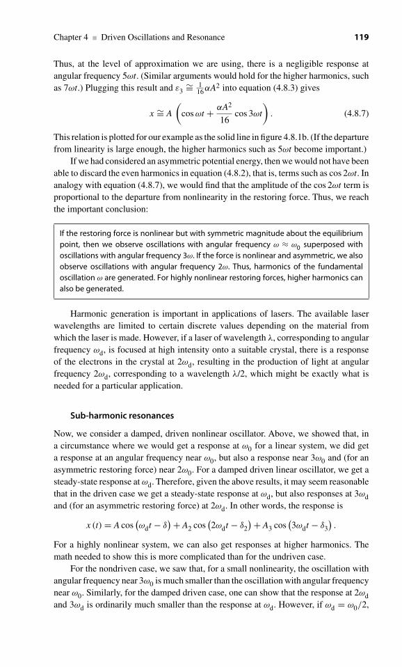
Chapter 4 ■ Driven Oscillations and Resonance 119
Thus, at the level of approximation we are using, there is a negligible response atangular frequency 5ωt. (Similar arguments would hold for the higher harmonics, suchas 7ωt.) Plugging this result and ε3
∼= 116αA2 into equation (4.8.3) gives
x ∼= A
(cos ωt + αA2
16cos 3ωt
). (4.8.7)
This relation is plotted for our example as the solid line in figure 4.8.1b. (If the departurefrom linearity is large enough, the higher harmonics such as 5ωt become important.)
If we had considered an asymmetric potential energy, then we would not have beenable to discard the even harmonics in equation (4.8.2), that is, terms such as cos 2ωt. Inanalogy with equation (4.8.7), we would find that the amplitude of the cos 2ωt term isproportional to the departure from nonlinearity in the restoring force. Thus, we reachthe important conclusion:
If the restoring force is nonlinear but with symmetric magnitude about the equilibriumpoint, then we observe oscillations with angular frequency ω ≈ ω0 superposed withoscillations with angular frequency 3ω. If the force is nonlinear and asymmetric, we alsoobserve oscillations with angular frequency 2ω. Thus, harmonics of the fundamentaloscillation ω are generated. For highly nonlinear restoring forces, higher harmonics canalso be generated.
Harmonic generation is important in applications of lasers. The available laserwavelengths are limited to certain discrete values depending on the material fromwhich the laser is made. However, if a laser of wavelength λ, corresponding to angularfrequency ωd, is focused at high intensity onto a suitable crystal, there is a responseof the electrons in the crystal at 2ωd, resulting in the production of light at angularfrequency 2ωd, corresponding to a wavelength λ/2, which might be exactly what isneeded for a particular application.
Sub-harmonic resonances
Now, we consider a damped, driven nonlinear oscillator. Above, we showed that, ina circumstance where we would get a response at ω0 for a linear system, we did geta response at an angular frequency near ω0, but also a response near 3ω0 and (for anasymmetric restoring force) near 2ω0. For a damped driven linear oscillator, we get asteady-state response at ωd. Therefore, given the above results, it may seem reasonablethat in the driven case we get a steady-state response at ωd, but also responses at 3ωdand (for an asymmetric restoring force) at 2ωd. In other words, the response is
x (t) = A cos(ωdt − δ
) + A2 cos(2ωdt − δ2
) + A3 cos(3ωdt − δ3
).
For a highly nonlinear system, we can also get responses at higher harmonics. Themath needed to show this is more complicated than for the undriven case.
For the nondriven case, we saw that, for a small nonlinearity, the oscillation withangular frequency near 3ω0 is much smaller than the oscillation with angular frequencynear ω0. Similarly, for the damped driven case, one can show that the response at 2ωdand 3ωd is ordinarily much smaller than the response at ωd. However, if ωd = ω0/2,

120 Waves and Oscillations
then the response at 2ωd = ω0 is amplified by the resonance of the system. If Q islarge, the response at 2ωd = ω0 can thus be significantly larger than the response atωd. Similar comments apply for ωd = ω0/3. Thus, we can excite the resonance of asystem with a drive force frequency below the resonant frequency.
Sub-harmonic resonances are often annoying. For example, parts of speakers inan audio system can be modeled as mass/spring oscillators. (Since all the parts are inequilibrium positions, we know that there are spring-like forces holding them there.)If the volume is turned up high, the sound drives the mechanical components of thespeaker at high amplitude, so that the nonlinear region of the restoring force becomesimportant. When the frequency of the sound is half or one third of the resonantfrequency of a part, it can be excited through the sub-harmonic resonance effect,resulting in an unpleasant buzz.
Mixing
A resistor has a linear current–voltage relationship:
V = IR ⇒ I = GV ,
where G ≡ 1/R is the conductance. If we apply the voltage
V = V1 cos ω1t + V2 cos ω2t (4.8.8)
to a resistor, nothing very exciting happens. The resulting current is simply
I = V/R = GV1 cos ω1t + GV2 cos ω2t.
However, now let’s consider a circuit element with a nonlinear current–voltagerelationship, such as
I = GV (1 + αV ) = GV + αGV2,
where α is a constant. (Note: the current as a function of voltage for any device canbe written as a Taylor series, so for anything other than a resistor there will be aterm proportional to V2 and/or V3. Thus, we need not be talking about a very exoticcomponent; something like a diode would exhibit the effects we discuss here).Applyingthe voltage (4.8.8) to this nonlinear device gives a current
I = GV1 cos ω1t + GV2 cos ω2t + αG(V1 cos ω1t + V2 cos ω2t
)2. (4.8.9)
It is the third term which is of most interest:
αG(V1 cos ω1t + V2 cos ω2t
)2
= αG(
V21 cos2 ω1t + 2V1V2 cos ω1t cos ω2t + V2
2 cos ω2t)
. (4.8.10)
Now, we use two trigonometric identities:
cos2 θ = 12 (1 + cos 2θ) and cos A cos B = 1
2 [cos (A + B) + cos (A − B)] .

Chapter 4 ■ Driven Oscillations and Resonance 121
Applying these to equation (4.8.10) gives
αG(V1 cos ω1t + V2 cos ω2t
)2 = αG
2
[V2
1 + V22 + V2
1 cos 2ω1t + V22 cos 2ω2t
+2V1V2 cos(ω1 + ω2
)t + 2V1V2 cos
(ω1 − ω2
)t].
Thus, the current has components that oscillate at ω1 and ω2 (as we can see fromequation (4.8.9), but also components that oscillate at 2ω1, 2ω2, ω1 +ω2, and ω1 −ω2.
It is these last two that are perhaps the most interesting. We could call them thesum angular frequency and the difference angular frequency. The difference angularfrequency plays the key role in the technique of “heterodyning,” which is used invirtually every radio receiver. In AM radio, the information to be transmitted is used asan envelope function for a “carrier wave.” The carrier wave must have a much higherfrequency (around 1 MHz) than the audio information (about 10 kHz). In FM radio,the information to be transmitted is instead used to control the frequency of the carrierwave; a variation in the audio wave causes a small change in the carrier frequency.In either case, inside the radio receiver, the signal from the antenna is mixed with thesignal from a “local oscillator,” which is simply a source of AC voltage at a frequencynear that of the carrier. The mixing occurs by applying both signals to a nonlinearelement, as described earlier. Because the frequency of the local oscillator is close tothat of the carrier wave, the difference frequency generated by the mixing is a muchlower frequency, and so this signal can more easily be processed by subsequent circuitsin the receiver.
The same mixing effects occur in a nonlinear oscillator that is driven by two forcesat angular frequencies ω1 and ω2; this results in a response that is the sum of functionsthat oscillate at 2ω1, 2ω2, ω1 + ω2, and ω1 − ω2, with amplitudes proportional tothe amplitudes of the drive forces. (The math required to show this for the caseof a nonlinear oscillator is more complicated than for the nonlinear circuit elementdescribed earlier.)
Sensitivity to initial conditions
For some systems with nonlinear restoring forces, one observes (for appropriate choicesof parameters) very complicated motion, even though the system itself is simple,and fully described by exact equations. In a system without a driving force, motioneventually ceases due to dissipation, but the final state of the system can be sensitiveto the tiniest changes in the initial conditions.
One example is the “magnetic pendulum,” consisting of a rigid pendulum armending in a small piece of iron, which hangs above a flat surface that has three identicalmagnets on it, as shown in the top part figure 4.8.2. One of the magnets is colored white,one black, and one gray. The piece of iron is attracted to each of the magnets, by a forceproportional to 1/r3. Thus, the end of the pendulum moves in response to a nonlinearforce. If the pendulum is started from rest near one of the magnets, it simply swingstoward the magnet, and oscillates around it until damping brings it to rest close to thatmagnet. Each of these three possible final resting points is called an “attractor.”
If the pendulum is released at rest at a point far away from any of the magnets,it follows a very complex trajectory. Eventually, it does come to rest at one of the
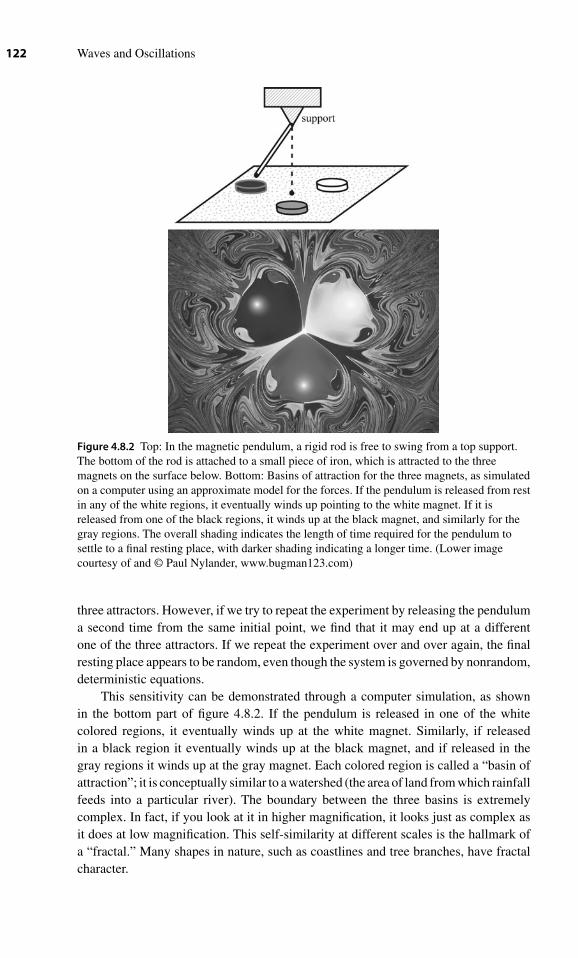
122 Waves and Oscillations
Figure 4.8.2 Top: In the magnetic pendulum, a rigid rod is free to swing from a top support.The bottom of the rod is attached to a small piece of iron, which is attracted to the threemagnets on the surface below. Bottom: Basins of attraction for the three magnets, as simulatedon a computer using an approximate model for the forces. If the pendulum is released from restin any of the white regions, it eventually winds up pointing to the white magnet. If it isreleased from one of the black regions, it winds up at the black magnet, and similarly for thegray regions. The overall shading indicates the length of time required for the pendulum tosettle to a final resting place, with darker shading indicating a longer time. (Lower imagecourtesy of and © Paul Nylander, www.bugman123.com)
three attractors. However, if we try to repeat the experiment by releasing the penduluma second time from the same initial point, we find that it may end up at a differentone of the three attractors. If we repeat the experiment over and over again, the finalresting place appears to be random, even though the system is governed by nonrandom,deterministic equations.
This sensitivity can be demonstrated through a computer simulation, as shownin the bottom part of figure 4.8.2. If the pendulum is released in one of the whitecolored regions, it eventually winds up at the white magnet. Similarly, if releasedin a black region it eventually winds up at the black magnet, and if released in thegray regions it winds up at the gray magnet. Each colored region is called a “basin ofattraction”; it is conceptually similar to a watershed (the area of land from which rainfallfeeds into a particular river). The boundary between the three basins is extremelycomplex. In fact, if you look at it in higher magnification, it looks just as complex asit does at low magnification. This self-similarity at different scales is the hallmark ofa “fractal.” Many shapes in nature, such as coastlines and tree branches, have fractalcharacter.

Chapter 4 ■ Driven Oscillations and Resonance 123
Figure 4.8.3 a: Free body diagram for a pendulum. b: Phase space plot for the damped,undriven pendulum.
Chaos
If a system with nonlinear restoring forces is also subjected to a periodic drive force,this can result in “chaos,” in which the system is not only extremely sensitive to initialconditions, but also is sensitive to minute perturbations at any later time. Even a tinyperturbation, such as a gentle puff of air, leads to a huge change in the later behavior.12
Furthermore, a chaotic system exhibits very complicated, ongoing nonperiodic motion,even though the drive force is periodic and the system is fully described by exactequations.
The damped, driven pendulum provides a good example of chaotic behavior.Let us find the exact version of the differential equation that governs this system.We showed in section 2.2 that, for small displacements, the restoring force for thependulum is proportional to displacement. However, this is an approximation; as shownin figure 4.8.3a, the restoring force is Fr = mg sin θ . Therefore, the restoring torque is
τ = −�mg sin θ.
12. This sensitivity to initial conditions and small perturbations is often referred to as the “butterflyeffect.” The name stems from a talk given in 1963 by one of the founding fathers of the field ofchaos. During the talk, Edward Lorenz said of chaos theory, “One meteorologist remarked thatif the theory were correct, one flap of a seagull’s wings would be enough to alter the course ofthe weather forever.” In later talks, the seagull evolved into a butterfly.

124 Waves and Oscillations
We include a viscous drag force
Fdrag = −bv = −b�θ,
which produces an associated torque
τdrag = −b�2θ .
Finally, we include a periodic driving torque τ0 cos ωdt. The angular version ofFTOT = mx is τTOT = I θ , which gives us
−�mg sin θ − b�2θ + τ0 cos ωdt = I θ .
For a simple pendulum, I = m�2, so that
− �mg sin θ − b�2θ + τ0 cos ωdt = m�2θ ⇔θ + γ θ + ω2
0 sin θ = τ0
m�2cos ωdt, (4.8.11)
with γ ≡ b/m and ω0 ≡ √g/�. This is a differential equation in the variable θ . Because
of the sin θ term, it is nonlinear, and therefore there is the possibility that, for appropriatechoices of parameters, the system will show chaotic behavior.
To visualize the behavior of the system, we need a couple of new tools. A phasespace plot is simply a plot with one axis for each variable that is time-dependent andthat is needed to specify the state of the system. (Such quantities are called “dynamicalvariables.”) For the case of zero driving torque, there are only two such variables: theangular position θ and the angular velocity θ . We can specify the state of the systementirely13 by giving the values of θ and θ . Thus, if we make a plot with θ on thehorizontal axis and θ on the vertical axis, then each point in the plot specifies a stateof the system. If we release the pendulum from rest at θ0, with zero driving torque, itfollows the phase space path shown in figure 4.8.3b, spiraling in toward rest at θ = 0.
One can show that, for a system to exhibit chaos, there must be at least threedynamical variables. When we turn on the driving torque, we get the third variable:ωdt, which is the argument of the cos ωdt term in equation (4.8.11), and is thereforecalled the “drive phase.” Now, in order to completely specify the state of the system,we need to specify θ , θ , and ωdt. You might ask, “Why not just use t as the dynamicalvariable instead of ωdt?” The answer is that we don’t actually need to know the timein order to specify the state of the system, but we do need to know the argument ofthe cos ωdt term; we do need to know whether the drive torque is at a maximum ora minimum, or somewhere in between, and whether it is increasing or decreasing atthe moment in question. Note that ωdt is an angular variable, measured in radians; thedrive torque has the same value at ωdt = 0 as it does at ωdt = 2π .
Since we now have three-dynamical variables, we need a three-dimensional phasespace to represent the system. The axis for ωdt need only run from 0 to 2π . Let’s now
13. Note that we need not also specify θ , since (for τ0 = 0) we can use equation (4.8.11) to calculateθ from θ and θ . Also note that specifying θ by itself is not enough to determine the state of thesystem. For example, if θ = 0, the pendulum could be swinging to the right or to the left.

Chapter 4 ■ Driven Oscillations and Resonance 125
Figure 4.8.4 a: Phase space plot for the damped, driven pendulum in steady state. The angle θ
is shown on the left-right axis, the angular velocity θ is shown on the axis that is more-or-lessperpendicular to the page, and the drive phase ωdt is shown on the vertical axis. The systemstarts at a maximum value of θ , as shown by point a and by the small picture labeled a, thenprogresses through points b–e. b: Similar plot for the pendulum with arbitrary initialconditions, leading to transient behavior that decays over time.
drive the pendulum at low amplitude (low enough that the nonlinearities are notimportant). We know that, in steady state, it follows simple harmonic motion:
θ = A cos(ωdt − δ
) ⇒ θ = −ωd A sin(ωdt − δ
).
As an example, we choose ωd = 215ω0, which gives δ ∼= 0. This means that θ = A
and θ = 0 at t = 0. The phase space plot for this steady-state behavior is shown infigure 4.8.4a; it is a helix that starts at the bottom. The phase space point representingthe system moves up the helix, and reaches the top of the helix at ωdt = 2π , which isequivalent to ωdt = 0, so the phase space point jumps down to the bottom of the helixand starts up again.
If we start the system with some arbitrary initial conditions, there will be sometransient behavior near t = 0, which damps away in time, until the system reachessteady state, as we explored in section 4.5; this behavior is shown in figure 4.8.4b.Once the transients damp away, the system returns to the helix phase space path thatrepresents the steady state. Therefore, this helix is the attractor for this system. It is a

126 Waves and Oscillations
Figure 4.8.5 a: Trajectory in the θ − θ plane for pendulum driven at low amplitude. b: APoincaré section of this motion. Parts c and f of the figure represent a higher amplitude motionof the pendulum, and so are at a larger scale than parts a and b. c: Trajectory in the θ − θ planefor higher drive torque, showing period doubling. d: A Poincaré section of this motion.e:Trajectory in the θ − θ plane for even higher drive torque, showing chaotic behavior. f: APoincaré section of this motion. g: A Poincaré section for a pendulum with less damping thanthe one shown in parts a–f, showing chaotic behavior. (Note that, unlike the other figures in theleft column, this is a Poincaré section rather than a phase space plot.) h: Zoom-in on the upperright part of the Poincaré section, showing that the complexity of the attractor does notdiminish as we zoom in. Parts c–h used with permission from Chaotic Dynamics: AnIntroduction, 2nd Ed., by G. L. Baker and J. P. Gollub, Cambridge University Press,Cambridge, 1996.
more complex attractor than the three points for the magnetic pendulum, and representsa dynamic behavior, but the idea is the same; it represents the behavior that the systemeventually settles into.
Because it is complicated to look at the three-dimensional phase space plot, oneoften instead just shows the projection onto the plane of the θ and θ axes (the θ − θ
plane). For the driven pendulum at low-drive amplitude in steady state shown infigure 4.8.4a, this projection is an ellipse, as shown in figure 4.8.5a.

Chapter 4 ■ Driven Oscillations and Resonance 127
Now, imagine that we illuminate the pendulum with a strobe lamp, which flashesonce per cycle of the drive torque. At each flash, we measure θ and θ , and plot thispoint in the θ − θ plane. The resulting plot is called a “Poincaré section.” For thesteady-state motion shown in figure 4.8.5a, the Poincaré section is simply a point, asshown in figure 4.8.5b. A single flash of the strobe is enough to create this particularPoincaré section, because the pendulum is in simple periodic motion. It is called asection because it is a slice through the three-dimensional phase space. We can chooseto have the strobe flashes occur at ωdt = 0, 2π , 4π , etc., in which case we get a slice atthe bottom of the cube shown in figure 4.8.4a. If instead we have the flashes occur atωdt = π , 3π , 5π , etc., then we get a slice halfway up the cube. By varying the timingof the flashes, we can map out different slices through the attractor. (Again, for thecase of low-drive amplitude, the attractor is the helix shown in figure 4.8.4a).
Next, we gradually increase the amplitude of the drive, τ0, while keeping ωd fixed.For our example, we now choose ωd = 2
3ω0. We discussed earlier in this section that,for small nonlinearity and a symmetric potential energy function, there is a responsenot only at ωd, but there is also a third harmonic response at 3ωd, which in this caseequals 2ω0. Therefore, there can be an interplay between this response and the naturalresonance angular frequency of the system, ω0. The period of the drive torque isT = 2π
ωd= 3
22πω0
. In a time interval 2T , the drive torque goes through exactly two cycles,the third harmonic response goes through exactly six cycles, while any oscillation atω0 goes through exactly three cycles. We can imagine therefore that the periodicity ofthe system could change, due to this interplay, from T to 2T , and this “period doubling”is indeed observed experimentally. The projection onto the θ − θ plane of the phase-space trajectory is shown in figure 4.8.5c, and a Poincaré section in figure 4.8.5d. Inthis case, two successive flashes of the strobe are needed to complete the Poincarésection; in subsequent flashes, the point representing the system alternates betweenthe first two points. As we increase the drive amplitude further, the system is driven tohigher amplitudes, and samples the nonlinearity of the restoring force more.Additionalcomplexities are added to the motion (such as the pendulum going “over the top”), andthe period gets longer, but the motion is still periodic.
Then, with a small additional increase in the drive amplitude, the motion suddenlychanges character. It is no longer periodic, as shown by the θ − θ plane plot infigure 4.8.5e, and the Poincaré section (figure 4.8.5f) becomes suddenly much morecomplex. In this case, many strobe flashes (in principle an infinite number) are neededto complete the Poincaré section, because the motion is not periodic. However, we seethat the motion is not completely random; even with a large number of flashes, manyparts of the Poincaré section remain blank.Again, the Poincaré section is a slice parallelto the θ − θ plane through the phase space attractor for the chaotic state (the equivalentof the helix of figure 4.8.4a). Just from this slice, we can tell that the attractor has amuch more complicated shape, and so it is called a “strange attractor.” If we attempt toexamine the Poincaré section it in more detail, by expanding the plot in a small region,it still looks just as complex, as suggested in figures 4.8.5g and h. Thus, the strangeattractor exhibits a fractal nature.
There are many plots, simulations, and animations relating to the chaotic pendulumavailable on the web; for a few suggestions, go to the web page for this text, and consultthe part for this chapter section.

128 Waves and Oscillations
Chaos is important in a remarkably wide range of fields, including economics,medicine, meteorology, physics, and chemistry. We have only scratched the surfaceof the rich and active fields of chaos and nonlinear dynamics. For further study, youmight begin with the very approachable text by Baker and Gollub.14
Concept and skill inventory for chapter 4
After reading this chapter, you should fully understand the following
terms:
Resonance (4.1)Steady state (4.1, 4.5)Amplitude resonance curve (4.1–4.2)Power resonance curve (4.3)FWHM (4.3)Superposition principle for driven systems (4.4)Transient (4.5)MRI (4.7)NMR (4.7)Magnetic moment (4.7)Precession (4.7)RF (4.7)Gyromagnetic ratio (4.7)Larmor frequency (4.7)Rotating reference frame (4.7)Spin up and spin down (4.7)Nonlinear differential equation (4.8)Harmonic generation (4.8)Frequency doubling (4.8)Subharmonic resonance (4.8)Mixing (4.8)Sensitivity to initial conditions (4.8)Dynamical variable (4.8)Basin of attraction (4.8)Phase space (4.8)Attractor (4.8)Strange attractor (4.8)Chaos (4.8)Fractal (4.8)
14. Chaotic Dynamics: An Introduction, 2nd Ed., by G. L. Baker and J. P. Gollub, CambridgeUniversity Press, Cambridge, 1996.

Chapter 4 ■ Driven Oscillations and Resonance 129
You should understand the following connections:
Motion of the support point and resulting drive force (4.1)Frequency of drive and frequency of steady-state response (4.1)Phase of drive and phase of response (4.1–4.2)Height of amplitude resonance curve and Q (4.2)Width of power resonance curve and γ (4.3)Height and width of power resonance curve (4.3)Average power supplied and average power dissipated in steady state (4.3)General solution for damped driven harmonic oscillator and solution for dampedoscillator (4.5)Damped driven mass/spring and driven RLC circuit (4.6)Protons and a child’s top (4.7)Torque and precession (4.7)Angular momentum and magnetic moment (4.7)Symmetry of potential energy curve and which harmonics are generated (4.8)
You should be familiar with the following additional concepts:
Advantages of expressing things in terms of dimensionless variables (4.2)
You should be able to:
Find the steady-state response amplitude and phase given information about theoscillator, the damping, and the drive (4.1–4.2)Find the response of a damped oscillator to superposed drive forces (4.4)Given the gyromagnetic ratio and Bapplied, calculate the RF frequency that producesNMR (4.7)Explain what a Poincaré section is (4.8)Explain what an attractor is (4.8)
In addition to all of the above, you should be able to combine the concepts
you’ve learned to address new situations.
Problems
Note: Additional problems are available on the website for this text.
Instructor: Ratings of problem difficulty, full solutions, and important additionalsupport materials are available on the website.
4.1 The following statement is incorrect. Provide a corrected version. “If youdrive a damped oscillator at a frequency other than ω0, the oscillator stilloscillates at its resonance frequency ω0. The amplitude of the responsedepends on how close the drive frequency is to the resonance frequency.”
4.2 Connection to current research: Frequency ModulationAFM. InAtomicForce Microscopy, a very sharp tip is used to “feel” the topography of the

130 Waves and Oscillations
sample by moving the tip in an x–y pattern over the region to be imagedwhile monitoring the force between the tip and sample. For the highestresolution images, the tip is not allowed to “touch” the sample. Instead, itis brought close enough to feel an attractive interaction (due to Van derWaals and other forces). As the tip is moved laterally over the sample,a feedback circuit adjusts the z-position of the tip to keep this attractiveforce constant. The record of the adjustments needed in z then gives thetopography of the sample. The tip is mounted at the end of a cantilever,which is set into oscillation, as shown schematically in figure 4.P.1a. (Theactual amplitude of vibration is much less than that shown; for the imagein figure 4.P.1b, the vibration amplitude was only 0.8 nm.) The attractiveforce between tip and sample is measured through its effect on the resonantfrequency of the cantilever/tip system. Ordinarily, this technique is used inultrahigh vacuum, and can give sub-atomic imaging resolution, as shown infigure 4.P.1b and c. For such an image, the measured forces are due to theinteractions of individual atomic orbitals!
The force of interaction between the tip and sample is shown schematicallyin figure 4.P.1d. The position of the tip x is measured relative to theequilibrium position in the absence of this interaction; note that downwardis defined as the positive direction for x. When the tip moves down (towardthe sample), the force is initially attractive (positive). As the tip starts to“touch” the surface, the force becomes repulsive (negative). A typical pointnear which the AFM might be operated is shown as x0. (a) Briefly explainwhy, near this point, we can model the force between tip and sample as
F ∼= F0 − kts
(x − x0
), where kts ≡ − dF
dx
∣∣∣x0
. (b) Note that kts functions like
a spring constant. It is negative because it acts oppositely to the spring ofthe cantilever; when the tip is closest to the sample (the point marked “A” inpart a of the figure), the cantilever pulls it up whereas the tip–sample force isattractive and so pulls it down. Let the spring constant of the cantilever be k,and the effective mass of the cantilever and tip be m. Explain why, if
∣∣kts
∣∣ � k,then the oscillation angular frequency is approximately ω ∼= ω0 +ω, where
ω0 ≡√
km and ω ≡ ω0
kts2k . (Therefore, by measuring the frequency shift,
one can measure the force of interaction between the tip and sample.)4.3 It should be clear that, for a damped driven harmonic oscillator that has
reached steady state, the average power supplied to the system by thedriving forces is equal to the average power dissipated by the damping force.However, for most drive frequencies there are parts of the cycle in whichpower flows from the oscillator to the entity providing the driving force (the“driver”), and other parts of the cycle during which power flows from thedriver into the oscillator. Thus, in general, the energy of the oscillator is notconstant during the cycle, even though its value averaged over the wholecycle is constant.Assume that k, m, and b are known. For what finite, nonzerovalue of ωd is the instantaneous power supplied by the driver exactly equalto the instantaneous power dissipated by the damping force at every instantin the cycle? Show your reasoning clearly. Hints: This means that the energy
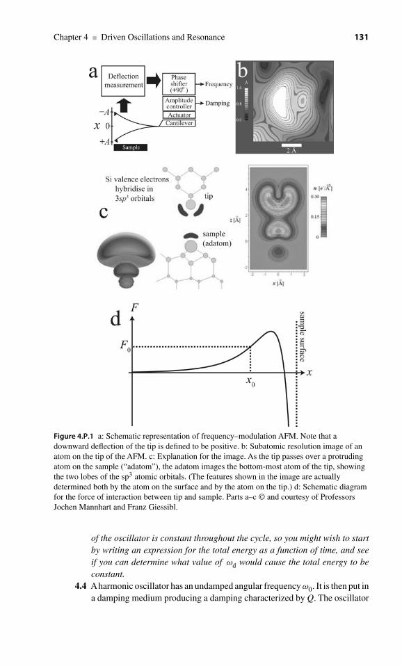
Chapter 4 ■ Driven Oscillations and Resonance 131
Figure 4.P.1 a: Schematic representation of frequency–modulation AFM. Note that adownward deflection of the tip is defined to be positive. b: Subatomic resolution image of anatom on the tip of the AFM. c: Explanation for the image. As the tip passes over a protrudingatom on the sample (“adatom”), the adatom images the bottom-most atom of the tip, showingthe two lobes of the sp3 atomic orbitals. (The features shown in the image are actuallydetermined both by the atom on the surface and by the atom on the tip.) d: Schematic diagramfor the force of interaction between tip and sample. Parts a–c © and courtesy of ProfessorsJochen Mannhart and Franz Giessibl.
of the oscillator is constant throughout the cycle, so you might wish to startby writing an expression for the total energy as a function of time, and seeif you can determine what value of ωd would cause the total energy to beconstant.
4.4 Aharmonic oscillator has an undamped angular frequency ω0. It is then put ina damping medium producing a damping characterized by Q. The oscillator

132 Waves and Oscillations
is driven at a frequency such that, in the steady state, the response x lagsbehind Fdrive by 45◦, meaning that the drive force reaches each peak a littleearlier than x does. The drive force amplitude is F0, and k is the effectivespring constant for the oscillator.
(a) Show that the response amplitude is A =√
2 F0Q2
k(√
1+4Q2−1) , and that
the dissipated power is Pdiss = ω0QF20
2k sin2 (ωdt − δ).
(b) Sketch qualitative graphs of the drive, response, potential energy,velocity, and dissipated power over one complete steady-state cycle.Align the graphs in a vertical column, or superpose the graphs, sothat the relationships between the five quantities are as clear aspossible.
4.5 Amass is subjected to a spring force Fspring = −kx, a damping force Fdamp =−bx, an oscillating drive force Fdrive = F0 cos ωdt, and an additionaldecaying force Fextra = De−β t , where D and β are positive constants.
(a) Write the differential equation for x that describes this system.(b) Write the simplest possible complex version of your DEQ from part
a, that is, the simplest complex DEQ whose real part is your DEQfrom part a.
(c) Show that z = Aeiϕeiωt is not a solution for your DEQ from part b,no matter what the values of A, ϕ, and ω are.
4.6 Driving a pendulum with vertical motion. Make your own simplependulum. (One easy way is to squeeze the tea out of a used teabag thathas a string.) First, get your pendulum swinging by holding the end ofthe string and moving your hand laterally. Find the resonant frequency,and measure it roughly. With the pendulum still swinging, see if you cankeep it going by moving your hand vertically instead of horizontally. If youexperiment enough, you should be able to do this, though it only works if thependulum is already swinging when you start moving your hand vertically.(a) What is the ratio of the frequency of your hand motion when you’removing your hand vertically divided by the frequency of your hand motionwhen you move your hand horizontally, assuming you drive the pendulum atresonance in both cases? (b) Explain your finding about the frequency ratioqualitatively.
4.7 Go to the website for this text, and under chapter 4 open the “Damped DrivenHarmonic Oscillator” applet. Use it to answer the following questions:
(a) To use this animation, select a quality factor (Q) of 15 with the sliderand then select a drive frequency by clicking on either of the twographs. Try some different values of Q and drive frequency. At whatdrive frequency do you get the greatest amplitude?
(b) The phase graph shows the phase relationship between the motionof the drive and the motion of the oscillator. What is the phaserelationship between the motion of the drive and the motion of the

Chapter 4 ■ Driven Oscillations and Resonance 133
oscillator at the point that you just found of greatest amplitude?How about at the two extremes of very low drive frequency andvery high drive frequencies?
(c) Now, click the check box labeled “Show Velocity” and observe thesmall velocity indicator to the right of the oscillator. What is itsphase relationship to the drive force at resonance? Why does thismake sense in terms of the power being delivered by the drive forceto the oscillator?
(d) Generally speaking, how does varying Q affect the amplitude andphase diagrams?
(e) This animation ignores “transients.” Because of this, what state ofa damped-driven harmonic oscillator system are we seeing?
(f) How does the steady-state response frequency compare to the drivefrequency at resonance? Well below resonance? Well above it?
4.8 Show that the peak of the amplitude resonance curve shown in figure 4.1.5
or 4.2.1 is at ωd = ω0
√1 − 1
2Q2 . Do not use a symbolic algebra program or
calculator.4.9 What, if anything, does the quality factor Q of a lightly damped mechanical
oscillator have to do with each of the following? Be brief, but as quantitativeas possible. (a) The rate at which the oscillator loses energy in the absenceof a driving force. (b) The “amplification factor” at resonance, that is, theamplitude of the oscillator’s motion when a driving force at the resonancefrequency is applied, as compared to the amplitude of motion when the sameamplitude driving force is applied at very low frequency. (c) The phase shiftat resonance. (Assume the damping is light enough that amplitude resonance,velocity resonance, acceleration resonance, and power resonance all occurat essentially the same frequency.) (d) The full width at half-maximum of the“power resonance curve,” that is, the graph of power absorbed as a functionof drive frequency.
4.10 A simple pendulum is made by attaching a steel sphere (ρ = 7,850 kg/m3)of radius 2.00 cm to the end of a thin string that is 1.00-m long. In thisproblem, take the resonant frequency to be
√g/L, where L is the distance
from the support point to the center of the sphere; assume that the dampingis light enough that the differences between ω0, ωv, and the peak angularfrequency for the amplitude response curve can be ignored. The support point(at the top of the string) is moved laterally (in the x-direction) in a sinusoidalpattern at the resonant frequency, with amplitude 1.00 μm = 1.00 × 10⁻⁶ m.What is the steady-state amplitude of the sphere’s motion in the x-direction?Assume that the air provides viscous damping, that is, that the airflow is notturbulent.)
4.11 Using the results of section 4.1, show explicitly that, in steady state, the netenergy provided by the drive force to a damped driven oscillator over oneperiod equals the energy dissipated by the damping force.
4.12 Steady-state response to a square wave. In section 8.4, we will show thatthe square wave (shown in black in figure 4.P.2) can be represented as an

134 Waves and Oscillations
Figure 4.P.2 Synthesizing a square wavefrom sinusoids.
infinite sum of sinusoids:
Square wave = cos ωt − cos 3ωt
3+ cos 5ωt
5− · · ·
The sum of the first three terms is shown in gray in the figure—you cansee that it roughly approximates the square wave. The preciseness of theapproximation improves as more terms are added. If a force with a squarewave time dependence is used as the drive force for a damped drivenharmonic oscillator, is the steady-state response a square wave? Explainyour answer thoroughly.
4.13 The curve of power dissipated versus drive frequency for a damped drivenoscillator is shown in figure 4.P.3. (The power dissipated averaged overa cycle in steady state is equal to the power absorbed from the driveforce.)
(a) What is the Q for this system?(b) The oscillator is driven at resonance until steady state is achieved.
The drive force is then suddenly turned off. About how long does ittake for the oscillations to die away? (Give your answer in seconds;all the numerical information you need is in the graph.)
(c) Now, instead, the oscillator is driven with fd = 850Hz. The driveforce is then turned off; thereafter, the oscillator continues tooscillate for a short time. At what frequency (approximately) does
Figure 4.P.3 A power resonance curve.

Chapter 4 ■ Driven Oscillations and Resonance 135
it oscillate during this part of the experiment (after the drive forceis turned off)? Explain briefly.
4.14 For the damped driven harmonic oscillator, find expressions for the adjustableconstants A0 and ϕ that appear in equation (4.5.2) in terms of the initialposition x0, the initial velocity x0, the steady-state amplitude A, the steady-state phase shift δ, ωv, and ωd. Do not use a symbolic algebra program orcalculator. Hints: Don’t expect the final result to be “neat.” You should beable to show that tan ϕ = B
D , where B and D are constants involving x0, x0,ωv, and γ . To find A0, you will need to find cos ϕ. To do this, draw a righttriangle with B and D as the two legs.
4.15 A weasel holds an object of mass m at its equilibrium position x = 0. Themass hangs from a spring of constant k in a medium which provides Fdamp =−bx. The support point for the spring is moving, with position given byxC = Ad cos ωdt. The angular drive frequency ωd happens to exactly equal√
km . (Don’t forget this, and its implications—otherwise, the math is a mess!)At t = 0, the weasel releases the mass, so that it can begin moving. Given
these initial conditions, what is the complete solution x(t)? Everything inyour solution should be expressed in terms of the symbols above only.However, you may make your life easier by defining symbols of your ownin terms of those above, then expressing your solution using these newsymbols.
4.16 An electrical engineer wishes to design an RLC oscillator, of the type shownin figure 4.6.1. The engineer wants the resonant response to be very strong,but also wants the system to respond strongly to a broad range of frequencies.Explain briefly why both goals can’t be achieved.
4.17 Radio station WJJZ has hired you to help design radio receivers to go inthe waiting rooms of doctors’ offices. Each of these radios is to receive theWJJZ broadcast only—there will be no “tuning” knob. One of your fellowengineers hands you part of the schematic diagram for the radio, shown in thetop part of figure 4.6.2. The input voltage to the LCR circuit from the antennais VIN = V0 cos ωdt, and the output voltage is taken across the capacitor(and then sent to the rest of the radio). “I already chose L = 0.1 μH,” hesays. “You pick out the values for R and C.” (Note: “μ” means “×10−6”).
(a) The broadcast frequency of WJJZ is f = 101.9 MHz. (Note: “M”means “ ×106”). What value of C should you pick so that the abovecircuit will resonate at this frequency? (Assume the circuit is verylightly damped.)
(b) Rival station WART broadcasts at f ′ = 101.5 MHz. The steady-state oscillation amplitude of your circuit (i.e., the amplitude ofVOUT) must be 100 times smaller at this frequency than at theWJJZ frequency, assuming equal drive (input) voltages for the twofrequencies. What is the required value for R ? Again, assume verylight damping. Your answer need only be correct to within a fewpercent. Hint: Don’t forget that q = CV ⇒ VOUT = q
C .

136 Waves and Oscillations
Figure 4.P.4 A parallel RLC oscillator.
(c) Of course, the WJJZ management would be happy if the amplitudefor WART is even less than 100 times below that for WJJZ. Bearingthis in mind, is the R you just calculated the maximum allowed Ror the minimum allowed R? Explain.
(d) What is the Q of your circuit?
4.18 The parallel RLC oscillator. Consider the circuit shown in figure 4.P.4.This is driven by applying a current I0 cos ωt, as shown. Assume the systemis underdamped. (a) What is the resonance frequency ω0? (b) What is theFWHM of the power resonance curve?
4.19 For this problem, the RLC oscillator shown in figure 4.6.1 is driven notsimply by the voltage V0 cos ωt, but instead by the more complicated voltageV1 cos ω1t + V2 sin ω2t. What is the charge on the capacitor, q (t), once thesystem reaches the steady state?
4.20 A patient is undergoing MRI. A particular proton in her brain experiences atotal applied magnetic field (including contributions from nearby electrons)of 1.50 T. The gyromagnetic ratio for a proton is γ = 2π · 42.576 MHz/T. (a)What frequency of RF radiation will this proton respond to most strongly?(b) For simplicity, in this part of the problem assume that the net magneticmoment and the net angular momentum of the protons in the local region ofthe brain can be treated by considering only their z-components. The mainmagnetic field in the MRI machine is applied in the z-direction. The magneticfield of the RF radiation is described by Brad = B0 cos ωt i. If B0 = 30.0μT,how long of an RF pulse should be applied to rotate the magnetization fromthe z-direction into the x–y plane?
4.21 Show that cos3 θ = 14 cos 3θ + 3
4 cos θ . (You will probably want to use asymbolic algebra program to do this.) This trigonometric identity is used insection 4.8.
4.22 Online exploration of a chaotic pendulum. Go to the entry for this problemon this book’s website, and follow the instructions there.

5 Symmetric Coupled Oscillators
and Hilbert Space
Gentlemen, I do not see that the sex of the candidate is an argument against heradmission as a privatdozent. After all, the senate is not a bathhouse.
– David Hilbert, arguing in favor of allowing Emmy Noether a position at theUniversity of Göttingen
5.1 Beats: An aside?
If you strike a tuning fork and listen, the resulting pressure variation at your ear issinusoidal. We might write the variation in pressure (relative to the average backgroundpressure) as
x1 = Re z1, where z1 = Aeiω1t .
Now, imagine that we strike two tuning forks of slightly different angular frequencies,ω1 and ω2. The resulting pressure variation at your ear is simply the sum of the
variations from the two forks. A/V: You can hear this right now by going to thisbook’s web page and clicking on the “listen to beats” link under this chapter section.This sound is remarkable – you perceive it as a single note (i.e., a single frequency)with an oscillating loudness! We can see how the loudness variations come aboutgraphically, as shown in figure 5.1.1a. This effect turns out to be of tremendousimportance for our future studies, so let’s see how it comes about mathematically.
To simplify the math, we’ll look at the case where the two amplitudes are thesame, that is,
z = z1 + z2 = A(eiω1t + eiω2t). (5.1.1)
It will help to define
ωe ≡ ω1 − ω2
2and ωav ≡ ω1 + ω2
2. (5.1.2)
(The subscript e is used for the first one because we will see that it is the angularfrequency of an envelope function.) You should verify right now that
ω1 = ωav + ωe and ω2 = ωav − ωe.
137

138 Waves and Oscillations
Figure 5.1.1 a: Two oscillations of slightly different frequencies (top) are added together(bottom). At first, the two waves are in phase, and so the sum has large amplitude. As timeprogresses, the two waves get out of phase, so the amplitude of the sum gets small. Withfurther passage of time, the waves start to get back into phase. b: A rapidly oscillating functionmultiplied by a slowly varying envelope function of period 2π/ωe (top) produces beats(bottom).
Therefore,
z = A[ei(ωav+ωe)t + ei(ωav−ωe)t
]
Your turn: Use the above and Euler’s equation (eiθ = cos θ + i sin θ ) to show that
z = 2Aeiωavt cos ωet
This means that
x = Re z = 2A︸︷︷︸constructiveinterferenceat maximum
cos ωavt︸ ︷︷ ︸rapid
oscillation
cos ωet︸ ︷︷ ︸slow oscillation
due to the transitionfrom constructive to
destructive interference(and back):
an envelope function
We see that x is the product of three terms: an overall amplitude, a rapid oscillation atthe average angular frequency, and a slow oscillation (corresponding to the oscillatingloudness). The slow oscillation is called an “envelope function,” because you can thinkof it as a time-dependent amplitude for the rapid oscillation, that is,
x = 2A cos ωet︸ ︷︷ ︸time-dependent
amplitude
cos ωavt︸ ︷︷ ︸rapid
oscillation
(5.1.3)
This multiplication is shown graphically in figure 5.1.1b. The slow variations inamplitude are called “beats,” and you’ll often hear people talking about one frequency“beating” against another, that is, the signals at two close frequencies combine to

Chapter 5 ■ Symmetric Coupled Oscillators and Hilbert Space 139
create beats. Following the usual convention, we define the beat period as the periodbetween maximum amplitudes, as shown, that is,
Tbeat ≡ π
ωe= 2π
ω1 − ω2(5.1.4)
Note that this is half the period of the envelope function. The beat frequency is thensimply
fbeat = 1
Tbeat= ω1 − ω2
2π⇒
fbeat = f1 − f2 (5.1.5)
Self-test (answer below1): Serious musicians sometimes use this phenomenon fortuning their instruments. Two guitar players are trying to bring their guitars to the samepitch. They both pluck their lowest string, and hear beats. One of the players beginsadjusting the pitch of her string, and the beat period gets shorter. Should she keepadjusting in this direction?Applet: Click on the “beats applets” link under this chapter section on this book’s webpage to see other ways of understanding beats.
5.2 Two symmetric coupled oscillators: Equations of motion
You probably have seen much of the material up to this point in previous courses, thoughnot at the same level of detail, nor with such a thrilling and masterful presentation.2
Now, we begin the truly new (and really neat!) stuff. We will begin by considering twocoupled oscillators, and this will lead directly to our treatment of waves (which we’llview as a large set of coupled oscillations), and to the most important ideas underlyingquantum mechanics.
The simplest and easiest-to-draw example of coupled oscillators is a set of twopendula, connected by a spring, as shown in figure 5.2.1a. To start with, we use pendulawith the same length and the same mass. Note that we define the position of each massrelative to its own equilibrium point, so that when the system is at equilibrium (bothpendula hanging straight down), we have x1 = 0 and x2 = 0. Also, for simplicity wewill ignore damping and driving forces for now.
If you displace mass 1 from equilibrium while holding mass 2 steady (at x2 = 0),
and then release both, you will observe a remarkable behavior. A/V: You can see a
1. If the beat period is getting shorter, the beat frequency is getting larger. According to equation(5.1.5), this means the two frequencies are getting farther apart. Therefore, she should stop andadjust in the other direction instead. Perfectly matched pitches will result in a very long beatperiod (in principle infinitely long).
2. I asked my wife for ideas on how to punch up the humor of this sentence, but her suggestionswere all too funny to include in a physics text.
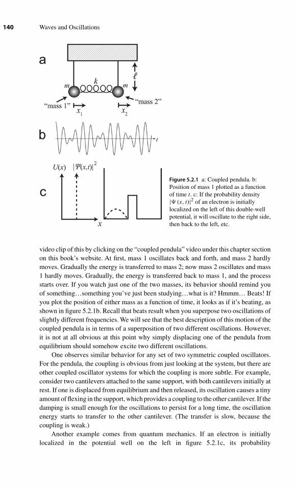
140 Waves and Oscillations
Figure 5.2.1 a: Coupled pendula. b:Position of mass 1 plotted as a functionof time t. c: If the probability density|� (x, t)|2 of an electron is initiallylocalized on the left of this double-wellpotential, it will oscillate to the right side,then back to the left, etc.
video clip of this by clicking on the “coupled pendula” video under this chapter sectionon this book’s website. At first, mass 1 oscillates back and forth, and mass 2 hardlymoves. Gradually the energy is transferred to mass 2; now mass 2 oscillates and mass1 hardly moves. Gradually, the energy is transferred back to mass 1, and the processstarts over. If you watch just one of the two masses, its behavior should remind youof something…something you’ve just been studying…what is it? Hmmm… Beats! Ifyou plot the position of either mass as a function of time, it looks as if it’s beating, asshown in figure 5.2.1b. Recall that beats result when you superpose two oscillations ofslightly different frequencies. We will see that the best description of this motion of thecoupled pendula is in terms of a superposition of two different oscillations. However,it is not at all obvious at this point why simply displacing one of the pendula fromequilibrium should somehow excite two different oscillations.
One observes similar behavior for any set of two symmetric coupled oscillators.For the pendula, the coupling is obvious from just looking at the system, but there areother coupled oscillator systems for which the coupling is more subtle. For example,consider two cantilevers attached to the same support, with both cantilevers initially atrest. If one is displaced from equilibrium and then released, its oscillation causes a tinyamount of flexing in the support, which provides a coupling to the other cantilever. If thedamping is small enough for the oscillations to persist for a long time, the oscillationenergy starts to transfer to the other cantilever. (The transfer is slow, because thecoupling is weak.)
Another example comes from quantum mechanics. If an electron is initiallylocalized in the potential well on the left in figure 5.2.1c, its probability

Chapter 5 ■ Symmetric Coupled Oscillators and Hilbert Space 141
density3 eventually moves entirely over to the right well, and then back to the left,just as the energy of the two coupled pendula moves back and forth.
Getting back to the example of the coupled pendula, our task (similar to those inthe previous chapters) is to find x1(t) and x2(t) given the initial conditions. We begin ourthree-step procedure, through instead of steps 2 and 3 we will use a different method,in section 5.3.
1. Write Newton’s second law for each object in the system:
Your turn: Convince yourself that the force due to the spring on mass 1 is given by
Fspring, 1 = −k(x1 − x2
).
Hint: First find the force when mass 1 is held at x1 = 0 but mass 2 is allowed to move.Then find the force when mass 2 is held at x2 = 0 but mass 1 is allowed to move.
The above equation shows mathematically that the force on mass 1 depends not onlyon the position of mass 1, but also on the position of mass 2, so that the motion ofthe two masses is “coupled.” The total force on mass 1 is the sum of the spring forceand the “pendulum force” discussed in chapter 3. Recall that, for small displacementsfrom equilibrium, the tension in the string and gravity combine to produce a spring-likeforce given by
Fpendulum = −mg
�x
Therefore, the total force on mass 1 is
F1 = −mg
�x1 − k
(x1 − x2
) = mx1
⇔ x1 + g
�x1 + k
m
(x1 − x2
) = 0. (5.2.1a)
Similarly, the differential equation governing the motion of mass 2 is
x2 + g
�x2 + k
m
(x2 − x1
) = 0. (5.2.1b)
These are a set of two DEQs, representing the motion of two objects. The equationsare “coupled” because x2 appears in the first equation and x1 appears in the secondequation. This mathematical coupling of the equations is a direct result of the physicalcoupling of the masses. The coupling makes the equations difficult to solve, becausewe must simultaneously find the solutions x1 (t) and x2 (t) for both equations. It wouldbe much easier to find solutions if we could decouple the equations, that is, if we couldfind a way to write two other second-order differential equations that also completelydescribe the system, but which aren’t coupled. There is a general recipe for doing this,and we will study it, but for this simple case we will use physical insight instead.
3. The concept of probability density was discussed in section 1.11.

142 Waves and Oscillations
5.3 Normal modes
If we could succeed in describing the system with two uncoupled differential equations,then (because they’re uncoupled), each would represent a completely independent typeof motion, without any energy transfer between the two. This would be analogous to thetwo pendula shown in figure 5.2.1a, but with no spring between. These two uncoupledoscillators are described by two uncoupled DEQs:
−mg
�x1 = mx1 ⇔ x1 + g
�x1 = 0
x2 + g
�x2 = 0
⎫⎪⎬⎪⎭ Two uncoupled DEQs (5.3.1)
In this analogy, we can set mass 1 moving, and no energy is ever transferred to mass 2.Mass 1 continues oscillating in a simple “steady-state” motion, that is, it oscillates withconstant amplitude.
For the coupled pendula, can we think of a way in which the system can movein a steady state, in which each mass oscillates with constant amplitude? We will callthis way of moving a “normal mode.” In fact, we need to think of two normal modes,since we know that we’ll need two second-order DEQs to describe the system. (Afterall, we started with two DEQs, equations 5.2.1a and b.)
One of these normal modes is easy to guess, as shown in figure 5.3.1. This iscalled the “pendulum mode”; the two masses swing in phase. Since x1 is alwaysequal to x2, the spring never gets stretched or compressed, so it never exerts anyforce. If there is no damping, the system would continue swinging in this modeforever.
Concept test: See if you can figure out the other normal mode for this system. In otherwords, figure out a different way in which the system can move forever in a steady state.Don’t look any further until you’ve put an honest effort into thinking about this.
This other normal mode is called the “breathing mode,” and is shown in figure 5.3.2a.This is a completely antisymmetrical motion. Therefore, if we excite this mode only,there is no way to generate the symmetrical motion that would lead to the pendulummode. Another way to understand why this mode would continue in a steady state isthat the center point of the spring never moves. Therefore, you could attach the center
Figure 5.3.1 In the pendulum mode, the system oscillates between these two configurations.Each mass oscillates with constant amplitude.

Chapter 5 ■ Symmetric Coupled Oscillators and Hilbert Space 143
Figure 5.3.2 a: In the breathingmode, the system oscillates
between these two configurations.Each mass oscillates with
constant amplitude. b: In thebreathing mode, the center point
of the spring doesn’t move, so wecould pretend that it’s attached to
a wall.
point to an immovable anchor without changing anything, turning the two pendula intotwo uncoupled oscillators moving in unison (though in opposite directions).
Now that we’ve found these two normal modes, let’s find the two differentialequations that describe them, and then see how they’re related to the original differentialequations 5.2.1a and b. We can characterize the pendulum mode by defining
sp ≡ 1√2
(x1 + x2
). (5.3.2)4
When the system moves in the pendulum mode, there is an oscillation of sp. If the
system is “purely” in the pendulum mode, then x1 = x2, so sp = √2x1 = √
2x2,so this definition might seem to be of little use. However, we will soon considermore complicated motions, involving a superposition of the pendulum mode andthe breathing mode, and then we will really need this definition. You can show inproblem 5.17 that sp always shows a simple harmonic oscillation, even when themotions of x1 and x2 are more complicated (because of a superposition of the twomodes). Therefore, sp is called the “normal mode coordinate” for the pendulummode.
In the pure pendulum mode, the spring never stretches, so the motion of eachpendulum is that of a simple pendulum. Therefore, we have
F1 = mx1 = −mg
�x1 ⇔ x1 + g
�x1 = 0.
System in pendulum mode
In the pendulum mode, we have sp = √2x1, so that sp = √
2 x1. Therefore, we couldjust as well write
sp + g
�sp = 0. (5.3.3)
This differential equation describes the motion of the pendulum mode. It has the form
of a simple harmonic oscillator DEQ, x + k
mx = 0. Therefore, the angular frequency
4. The factor of 1/√
2 in this definition might seem unneeded, but eventually it will make thingseasier to think about.

144 Waves and Oscillations
of oscillation is given by the equivalent of ω =√
k
m:
ωp =√
g
�(5.3.4)
There is a different way of deriving the DEQ (5.3.3), which is quite revealing. Inspiredby the definition of sp, equation (5.3.2), we try adding together equations (5.2.1), after
multiplying each by 1/√
2:
1√2
[x1 + g
�x1 + k
m
(x1 − x2
) = 0
](5.2.1a)
+ 1√2
[x2 + g
�x2 + k
m
(x2 − x1
) = 0
](5.2.1b)
______________________________
1√2
[(x1 + x2
) + g
�
(x1 + x2
) = 0]
Using the definition sp = 1√2
(x1 + x2), this becomes
sp + g
�sp = 0, (5.3.5)
which is just the same as equation (5.3.3). Note that to do this second derivation, wedid not require that the system be in pendulum mode, so this equation must alwayshold, whether the system is in the pendulum mode, the breathing mode, or some morecomplicated motion.
Now, for the breathing mode. We can characterize the breathing mode by defining
sb ≡ 1√2
(x1 − x2
). (5.3.6)
When the system moves in the breathing mode, sb oscillates. (If the system is “purely”in the breathing mode, then x2 = −x1, so sb = √
2x1.) Again, you can show inproblem 5.17 that, even when the system is in a superposition of the two modes,sb still moves in simple harmonic fashion. Therefore, sb is called the normal modecoordinate for the breathing mode.
Since the center of the spring never moves, we could imagine replacing the righthalf of the apparatus by a brick wall, as shown in figure 5.3.2b; this would not affect themotion of mass 1. Therefore, the motion of the left mass is that of a simple harmonicoscillator; we just need to figure out the effective spring constant. (Of course, oncewe have found the motion of the left mass, we can easily find the motion of the rightmass, since, in the breathing mode, x2 = −x1.) There are two forces acting on the left
mass: the “pendulum force,” with effective spring constantmg
�, and the force from the
spring, which is effectively half its original length. Recall from section 2.3 that whenthe length of a spring is cut in half, the spring constant is doubled. Applying this to our

Chapter 5 ■ Symmetric Coupled Oscillators and Hilbert Space 145
analysis of the breathing mode, the effective total spring constant ismg
�+ 2k, so that
F1 = mx1 = −(mg
�+ 2k
)x1 ⇔ x1 +
(g
�+ 2k
m
)x1 = 0. (5.3.7)
System in breathing mode
Since (in the breathing mode), we have sb = √2x1, we could just as well write
sb +(
g
�+ 2k
m
)sb = 0 (5.3.8)
This differential equation describes the motion of the breathing mode. It has the form
of a simple harmonic oscillator DEQ, x + k
mx = 0. Therefore, the angular frequency
of oscillation is given by the equivalent of ω =√
k
m:
ωb =√
g
�+ 2k
m(5.3.9)
We see that the breathing mode has a higher frequency than the pendulum mode,and that the difference in frequencies increases with the strength of the coupling,represented by k. We’ll discuss this important feature at length in section 5.7.
As for the pendulum mode, there is a different, more mathematical way of derivingthe breathing mode. Inspired by the definition of sb, equation (5.3.6), we try subtractingequations (5.2.1), after multiplying each by 1/
√2:
1√2
[x1 + g
�x1 + k
m
(x1 − x2
) = 0
](5.2.1a)
− 1√2
[x2 + g
�x2 + k
m
(x2 − x1
) = 0
](5.2.1b)
_________________________________________
1√2
[(x1 − x2
) + g
�
(x1 − x2
) + 2k
m
(x1 − x2
) = 0
]
Using the definition sb = 1√2
(x1 − x2), this becomes
sb +(
g
�+ 2k
m
)sb = 0, (5.3.10)
which is just the same as equation (5.3.8). Again, we did not need to require thatthe system be in breathing mode, so this equation must always hold, whether thesystem is in the pendulum mode, the breathing mode, or some more complicatedmotion.

146 Waves and Oscillations
Recap: We began by describing the system of two coupled pendula in terms of themotion of each mass, as described by the pair of differential equations
DEQs describing the pendulum bobs:
⎧⎪⎨⎪⎩
(5.2.1a): x1 + g
�x1 + k
m
(x1 − x2
) = 0
(5.2.1b): x2 + g
�x2 + k
m
(x2 − x1
) = 0
The motion of each pendulum bob can be complicated, with energy being transferredback and forth between the two bobs, and it is difficult to solve these differentialequations because they are coupled.
Using physical insight, we discovered two simpler ways in which the system couldmove, the “pendulum mode” and the “breathing mode.” When the system is in one ofthese modes, the behavior is a simple oscillation, with no transfer of energy from onemode to the other. We showed that the behavior of these two modes could be describedby the pair of differential equations
DEQs describing the normal modes:
⎧⎪⎨⎪⎩
(5.3.5) : sp + g
�sp = 0
(5.3.10) : sb +(
g
�+ 2k
m
)sb = 0
where
sp ≡ 1√2
(x1 + x2
)and sb ≡ 1√
2
(x1 − x2
)are the “normal mode coordinates.” Since these DEQs have the form of simple harmonicoscillators, we could easily see that
ωp =√
g
�(5.3.4)
and
ωb =√
g
�+ 2k
m(5.3.9)
We showed that the second pair of DEQs could be derived from the first simply byadding or subtracting them.
Note that we don’t really need to continue with steps 2 and 3 of our three-step procedurefor solving the differential equations, since we’ve just shown that the motion of thissystem can be understood in terms of two simple oscillators (the pendulum mode andthe breathing mode). However, we do need to get a better understanding of how thesemodes combine to produce the complex behavior of the pendulum bobs that you sawin the video.
5.4 Superposing normal modes
Because the pair of DEQs (5.3.5) and (5.3.10) that describes the two normal modes canbe derived from the pair of DEQs (5.2.1a) and (5.2.1b) that describes the motion of thetwo pendulum bobs, each pair represents just as good a way of describing the complete

Chapter 5 ■ Symmetric Coupled Oscillators and Hilbert Space 147
Figure 5.4.1 a: Any initial condition can be expressed as an appropriately weightedsuperposition of the normal modes. b: Express this initial condition as a weightedsuperposition of the normal modes.
behavior of the system as does the other. However, because each normal mode acts asa simple oscillator (completely independent of the other mode), it is easy to predict itsbehavior in time.
By choosing the phases and amplitudes of the two modes correctly, we can createany desired initial condition for the two pendulum bobs. For example, as shown infigure 5.4.1a, we can create the initial condition shown in the video clip (the oneyou watched at the beginning of section 5.2) by adding together equal amounts ofpendulum and breathing modes.
After we let go, the pendulum and breathing modes oscillate independently.For such a mixture of modes, we can’t directly observe the oscillations of eachmode. Instead, we see the effect of the combination of both modes on each of thetwo masses:
sp ≡ 1√2
(x1 + x2
)and sb ≡ 1√
2
(x1 − x2
)⇔ x1 = 1√
2
(sp + sb
)and x2 = 1√
2
(sp − sb
)(5.4.1)
A remarkable insight: Thus, the “beating” behavior that we observe, say for mass 1,
is due to the superposition of the pendulum mode ( at angular frequency ωp =√
g
�
)
and the breathing mode (at a different angular frequency, ωb =√
g
�+ 2k
m
)! (Recall
from section 5.1 that superposing two oscillations of equal amplitude but differentfrequencies results in beating.)
In fact, we now understand that any behavior of the system can be understood interms of a superposition of the two normal modes.
Your turn: Describe the initial condition shown in figure 5.4.1b (both pendula areinitially at rest) in terms of a superposition of the two normal modes, in a way similar tofigure 5.4.1a.

148 Waves and Oscillations
Example: A set of coupled pendula has m = 0.10 kg for both masses, but k and � areunknown. At t = 0, the left mass is held at x1 = 2.0 cm and the right mass is held atx2 = 0 cm. The masses are then released. At first, the left mass oscillates with a periodof about 1.1 s, and the right mass is nearly motionless. At t = 10 s, the two masses areoscillating with approximately equal amplitudes. At t = 20 s, the right mass is oscillatingstrongly, and the left mass is nearly motionless. At t = 30 s, the two masses are oscillatingwith approximately equal amplitude. At t = 40 s, the left mass is oscillating strongly, andthe right mass is nearly motionless. Find approximate values for k and �.Solution: This beating behavior is caused by mixing together the two normal modes,with their two characteristic frequencies. For example, the motion of the left mass isa superposition of two different sinusoids of angular frequencies ωb and ωp, and thevariations in the amplitude for the left pendulum are due to the beating that results fromthis superposition. The time between maximum amplitudes (e.g., for the left pendulum)
is 40 s, so that the beat frequency is fbeat = 140
Hz .
We have that
(5.1.5) : fbeat = f1 − f2,
where in this case f1 = fb = ωb
2πand f2 = fp = ωp
2π. So,
fb − fp = 140
Hz ⇒ ωb − ωp =( π
20rad/s
). (5.4.2)
The period of the fast oscillations is given by Tfast = 2π
ωav= 2π
ωb + ωp
2
= 4π
ωb + ωp,
and we’re told that this equals 1.1 s for this example. Therefore, (1.1 s) = 4π
ωb + ωp⇔
ωb + ωp =(
4π
1.1rad/s
). Subtracting this from equation (5.4.2) gives
ωb − ωp =( π
20rad/s
)−
[ωb + ωp =
(4π
1.1rad/s
)]
______________________
−2ωp =( π
20rad/s
)−
(4π
1.1rad/s
)⇔
ωp = 5.6 rad/s =√
g
�
⇒ � = 32 cm
Finally,
ωb − ωp = π
20rad/s ⇒ ωb = 5.7 rad/s
ωb =√
g
�+ 2k
m⇒ k = m
2
(ω2
b − g
�
)⇒ k = 0.088 N/m

Chapter 5 ■ Symmetric Coupled Oscillators and Hilbert Space 149
5.5 Normal mode analysis, and normal modes as an alternatedescription of reality
The breathing mode and the pendulum mode are the two normal modes of the coupledpendulum system. We will see that we can find similar normal modes even for verycomplicated systems of many masses interacting through many different forces. Allthese normal modes share the characteristics of the breathing and pendulum modesshown above, leading us to the definition:
Definition of a normal mode: A way in which the system can move in a steady state,in which all parts of the system move with the same frequency. The parts may havedifferent (perhaps zero or negative) amplitudes.
Given any set of initial conditions, we can determine the fractions of pendulum-modeand breathing-mode which are needed to produce those initial conditions. This processis called “normal mode analysis.” We can then use these normal mode amplitudes todetermine the future behavior of the system as a function of time:
Normal mode analysis:
1. Express the initial state of the system in terms of a superposition of the normalmodes, with an appropriate amplitude and phase for each mode.
2. Write the time dependent expressions for each normal mode coordinate,
e.g. sp = Re[Apei(ωpt+ϕp)
]3. If desired, form the appropriate combination of the normal mode coordinates to
find the positions of the masses (x1, x2, etc.)
For now, we will only consider situations in which the initial velocities are zero, sincethis makes the math easier and shows the important ideas. However, we will treat themore general case later in this chapter. It is easiest to explain normal mode analysiswith an example:
Core example: A set of coupled pendula has m = 0.10 kg, � = 0.15 m, and k = 5.0 N/m.At t = 0, the left mass is held at x1 = 1.0 cm and the right mass is held at x2 = 3.0 cm.The masses are then released. What is the position of mass 1 at t = 5.0 s?Solution: First we make the normal modes description of the system. As we saw inchapter 1, for a single oscillator that begins at rest, the initial position is equal to theamplitude of the motion. Similarly in this case, because the initial velocities are zero,the amplitude for each normal mode is equal to the initial value of the normal mode
coordinate,5 as defined by sp ≡ 1√2
(x1 + x2
)and sb ≡ 1√
2
(x1 − x2
).
continued
5. You might be concerned that the two modes might have nonzero initial velocities sp0and sb0which, when added together, could produce zero initial velocity for both pendula.

150 Waves and Oscillations
Plugging in the initial values of x1 and x2, we get sp = 4.0√2
cm = 2√
2 cm and sb = − 2.0√2
cm = −√2 cm. Each mode acts as an independent oscillator. Since the initial velocities are
zero, the phase factor ϕ in the solution s = Re[Aei(ωt+ϕ)
]is zero (as we saw in chapter 1),
so we can simply use s = A cos ωt. So, we have:
sp = (2√
2 cm)
cos ωpt and sb = (−√2 cm
)cos ωbt.
From equation (5.4.1), we have x1 = 1√2
(sp + sb
), so
x1 = (2 cm) cos ωpt − (1 cm) cos ωbt.
The angular frequencies of the normal modes are ωp =√
g
�= 8.1 rad/s and ωb =√
g
�+ 2k
m= 13 rad/s. Plugging these and t = 5.0 s into the above expression for x1
gives x1(t = 5.0 s) = −1.9 cm.
Why do we care so much about describing things in terms of normal modes? Thereare several reasons. First, as shown in the above “core by example” section, and as we’llsee as we progress through the book, the normal modes description provides by far theeasiest way of describing the behavior of a complicated system as a function of time,given the initial conditions. Secondly, our two most important senses, sight and hearing,perceive the world in a way that is closely related to normal modes. For example, whenyou hear a musical note being played, you don’t perceive a rapid oscillation of airpressure, but rather you hear a single pitch. When you see something that emits bluelight, you don’t perceive a rapidly oscillating electric field; instead, you see “blue.”Normal modes are also very important in understanding the spectra of chemicals; theinfrared spectrum reveals the frequencies of the vibrational normal modes.
Finally, the normal mode picture presents an alternate, and a very powerful,way of looking at the world. We will see that, for systems in which the motion isone-dimensional, the number of normal modes is equal to the number of particles.For example, in the two-pendulum system there were two normal modes. In a threependulum system, there would be three normal modes, etc. For each system, we caneither choose to describe the motion of each particle, or we can instead choose todescribe the motion of each normal mode. In a somewhat fantastic analogy, imaginetrying to completely describe a person. One way of doing it (analogous to describing thepositions of the two masses in our coupled pendula) would be to specify the positionsand velocities of all the electrons and nuclei that make up the person. But, instead,we might say, “This person is a mixture of 40% Hillary Clinton, 20% Frank Sinatra,20% Snoop Dogg, and 20% Julia Roberts.” Such a description would be similar to
However, for the pendulum mode the velocities of the two pendula are always equal, whilefor the breathing mode they are always opposite. Therefore, while it is possible to add cancellingvelocities for one of the two pendula, the velocities for the other would not cancel. The only wayto get zero initial velocity for both pendula is to have zero initial velocity for both modes.

Chapter 5 ■ Symmetric Coupled Oscillators and Hilbert Space 151
the normal modes way of describing the coupled pendula—the system is described interms of its archetypical behaviors. Such a description places no limits on the system,and does not require any less information (to describe an arbitrary person in termsof personality archetypes might require 1025 different archetypes), but is often morerevealing.
Energy of a superposition state
By equation (5.4.1), x1 = 1√2
(sp + sb
). So, when the system is purely in the pendulum
mode, the amplitude of the left pendulum bob isAp√
2, where Ap is the amplitude of the
pendulum mode, that is, the amplitude of sp. Therefore, the energy of the left bob is
1
2keff
( Ap√2
)2
, where the effective spring constant keff is entirely due to the “pendulum
force,” so that keff = mg
�. Since ωp =
√g
�, we could also write that the energy of the
left bob is 14 mω2
pA2p. The right bob has the same amount of energy, so that the total
energy is 12 mω2
pA2p. For convenience, we define Ep ≡ 1
2 mω2p (1 m)2; this is the energy
the pendulum mode would have for an amplitude of 1 m. Using this, the total energy
of the system in the pure pendulum mode can be expressed asA2
p
(1 m)2Ep.
If instead the system is in a pure breathing mode, then identical arguments show
that the total energy isA2
b
(1 m)2Eb, where Ab is the amplitude of motion of the left bob
in this breathing mode (which of course is the same as that of the right bob), andEb ≡ 1
2 mω2b (1 m)2 is the energy the mode would have for an amplitude of 1 m.
Now, let’s consider the energy when the system is in a state in which the twomodes are superposed. Since each mode can be considered as a completely independentoscillator, the total energy is simply the sum of the energies of the two modes, that is,
ETOT = A2p
(1 m)2Ep + A2
b
(1 m)2Eb (5.5.1)
We see that this is a sort of weighted sum, with the weights given by the squares of theamplitudes of each mode. We’ll see in the next few pages that this is closely related tothe energy of a quantum mechanical system that is in a superposition of two quantumstates.
Analogy between quantum superpositions
and normal mode superpositions
In quantum mechanics, normal modes play an absolutely central role. For example,each electron in an atom can be in one of several “quantum states,” labeled 1s, 2s, 2p,etc. Each of these states is a different normal mode for the electron. For a quantummechanical particle, there is a simple relationship between the total energy of the

152 Waves and Oscillations
particle and the angular frequency of oscillation:
E = hω,
where h ≡ h
2π. (Both h ≈ 1.055 × 10⁻³⁴ J s and h ≈ 6.63 × 10⁻³⁴ J s are called
“Planck’s constant.”) Therefore, each normal mode in quantum mechanics not only hasa characteristic angular frequency of oscillation, but also a corresponding energy. Thisexplains why the normal modes of a quantum system are called “energy eigenstates.”(“Eigen” means “characteristic” in German.) When the system is in one of these energyeigenstates, the quantum mechanical wavefunction � oscillates at the same frequencyat all points, just as the two pendula oscillate at the same frequency when the systemis in the pendulum mode (or the breathing mode). Just as in the coupled pendulumsystem, it is also possible to add together or superpose energy eigenstates to createmore complicated states. For example, say that �a represents a state with energy Ea,and �b represents a state with energy Eb. We could create a state with a superpositionof these two:
�mix =(
Aaeiϕa)
�a +(
Abeiϕb)
�b
Here, we have explicitly indicated the amplitudes Aa and Ab being used in thesuperposition, as well as the phases ϕa and ϕb. The quantum mechanical wavefunctionis inherently complex (!), so we don’t take the real part. This mixed state is exactlyanalogous to mixing together a pendulum mode of amplitude Ap and a breathing modeof amplitude Ab, for the coupled pendulum system.
Just as the energy in the coupled pendulum mixed state “sloshes” back and forthbetween the two pendula, the probability distribution for an electron in such a quantumstate is complicated, and the peak of probability “sloshes around” from one place toanother.
However, there is one area in which this otherwise very good analogy doesn’t work.If you measure the energy of the electron in this mixed quantum state, you always getEa or Eb, and never anything in between. This indeed is a “quantum mystery,” one thatyou will learn more about elsewhere, and one that has no analogy in the classical world.However, the probability of measuring energy Ea turns out to be A2
a , and the probabilityof measuring Eb turns out to be A2
b. Therefore, if you could prepare a million identicalelectrons, all initially in this same superposed state, and measure their energies, thenthe average energy of all these measurements would be
Eaverage = A2aEa + A2
bEb
The average energy, defined in this way, is called the “expectation value” of theenergy. (This is somewhat of a misnomer, since we don’t actually expect any singlemeasurement to match the expectation value. Rather, each single measurement willyield either Ea or Eb.) Comparing this with equation 5.5.1 shows that there is aclose analogy between the classical energy of the coupled pendulum system and theexpectation value of the energy for the quantum mechanical system.

Chapter 5 ■ Symmetric Coupled Oscillators and Hilbert Space 153
5.6 Hilbert space and bra-ket notation
There is a powerful way of thinking about superposing normal modes to create morecomplicated behavior, or the inverse operation of analyzing complicated behavior intoits simpler normal mode components.Again, for now we restrict ourselves to situationsin which both pendula have zero initial velocity. We could then visualize all the possibleinitial conditions as points or vectors on a plane, with the initial position of mass 1,x10, as the horizontal axis, and the initial position of mass 2, x20, on the vertical axis.Choosing a point in this plane, that is, choosing a set of initial conditions, completelyspecifies the behavior of the system for all subsequent times, as shown in the exampleof figure 5.6.1.
This plane is the simplest example of a Hilbert space6; so far there is not muchremarkable about it, but if we define things carefully we can generalize to much morecomplicated Hilbert spaces, which can be used to describe much more complicatedsystems, and we will gain enormous power! Mwah hah hah!!
Ahem. For example, if we had three masses in the system, we would need athree-dimensional Hilbert space to represent all the possible initial states of the system(again, sticking for now with the requirement that all the initial velocities be zero).If we had four masses, we would need a four-dimensional Hilbert space. If we had100 masses, we would need a 100-dimensional Hilbert space. If we want to describea continuous system, such as a rope, we could divide it up into an infinite number ofinfinitesimally small masses; we would need an infinite-dimensional Hilbert space todescribe such a system. Choosing one point/vector in such a space would correspondto specifying one coordinate along each of the infinite number of axes which define thespace. This infinite list of numbers is basically the same as a function; to completelydefine a function, you must define the value of the function at an infinite number ofpoints along the x-axis. So, each different point in an infinite-dimensional Hilbert spacesignifies a different function.
Figure 5.6.1 If we require theinitial velocities of both pendula tobe zero, then any initial conditioncan be depicted as a vector on the
plane shown in the right part of thefigure. The vector can be specifiedin column matrix format, with x10
in the top line and x20 in thebottom line.
6. The general definition of Hilbert space is a vector space with a defined “inner product”. Theinner product is a rule for combining two vectors to create a new quantity; for ordinary vectors inthree-dimensional space, the dot product is the inner product. Formally, a Hilbert space must be“complete” in a sense that is carefully defined by mathematicians, but this restriction is seldomimportant in physics.
154 Waves and Oscillations
But, for now, let’s stick to our two-dimensional Hilbert space that describes oursystem of two coupled pendula. Each vector in this space can be represented as acolumn matrix, with the top entry showing the component along the x10 axis and thebottom entry showing the component along the x20 axis, as shown in the figure. Thisway of representing vectors may be new to you; it works well when you need tomultiply a vector by a matrix, which we’ll do in chapter 6.
Let’s see how vector multiplication works in this notation. Here’s the way you’reused to taking dot products:
A · B = AxBx + AyBy. (5.6.1)
However, eventually (once we allow the initial velocities to be nonzero) we will need todeal with vectors that have complex components. For such vectors, the above definitionmust be modified. We want the dot product of any vector with itself to equal the squareof the length of the vector. This should be real, but
A · A = AxAx + AyAy
isn’t real if Ax or Ay is complex. Therefore, we instead define an extended version ofthe dot product:
A · B ≡ A∗xBx + A∗
yBy, (5.6.2)
where the ∗ indicates “complex conjugate.” Recall from section 1.8 that, to take thecomplex conjugate of any number, you simply replace any occurrence of i by −i. Forexample, if C = a + ib = Aeiϕ , then C∗ = a − ib = Ae−iϕ . Thus, equation (5.6.2) isthe same as equation (5.6.1) if the components are real. The complex conjugate makesit easy to find the magnitude of a complex number; if C = a + ib = Aeiϕ , then
Cartesian version: CC∗ = (a + ib) (a − ib) = a2 + b2 = |C|2
Polar version: CC∗ =(
Aeiϕ) (
Ae−iϕ)
= A2
Using the extended definition of the dot product, equation (5.6.2), we have
A · A = A∗xAx + A∗
yAy = ∣∣Ax
∣∣2 + ∣∣Ay
∣∣2,which is thus guaranteed to be real.
In the language of Hilbert space, we refer to dot products as “inner products.”To take the inner product of two vectors using matrix notation, we must first take theadjoint (also called the “Hermitian transpose” or “Hermitian conjugate”) of the one onthe left. Taking the adjoint means: write the matrix as a row instead of a column, andtake the complex conjugate of the entries. Here’s how this works:
A ≡(
A1A2
)⇒ adjoint of A is A† ≡ (
A∗1 A∗
2
),
where the † superscript means “adjoint.” The next step in taking the inner product ofA and B is to multiply A† with B using the rules of matrix multiplication. We’ll reviewthe full rules later. For now, we simply multiply the left entry of A† by the top entry of

Chapter 5 ■ Symmetric Coupled Oscillators and Hilbert Space 155
B and add this to the product of the right entry of A† and the bottom entry of B:
B ≡(
B1B2
)Inner product of A and B = (
A∗1 A∗
2
) (B1B2
)= A∗
1B1 + A∗2B2. (5.6.3)
This gives the same result as the extended definition of the dot product, equation (5.6.2).(Recall that, for now, all the vectors in our Hilbert space are real, but we want to makefully general definitions.)
Bra-ket notation In 1930, Paul Dirac introduced a wonderful notation that simplfiesthe writing of inner products; the advantages are not immediately obvious, but thisnotation is almost universally used for quantum mechanics, so you may as well begingetting used to it. Instead of writing a vector in Hilbert space as A or �A, we insteadwrite it as |A〉. The “|〉” that surrounds the “A” plays the same role as the arrow in�A – it simply tells you that the quantity is a vector. (In fact you can see that the
“|〉” sort of looks like an arrow.) A vector written with this new notation is called a“ket” – part of a little physics joke, as you’ll see. Thus, we write
|A〉 =(
A1A2
)
The adjoint of |A〉 is written 〈A| – this is called a “bra”:
〈A| ≡(A∗
1 A∗2
)Finally, the inner product of the vectors |A〉 and |B〉 is written 〈A | B〉:
|B〉 =(
B1B2
)
〈A | B〉 = (A∗1 A∗
2)
(B1B2
)= A∗
1B1 + A∗2B2.
Because this brings together the “bra” 〈A| with the “ket”|B〉, it forms a “bra-ket,”or bracket. Get it? Heh, heh.
Now, that you’re done rolling in the aisles, let’s see if you really did get it.
Concept test: If the ket |A〉 is given by |A〉 =(
2−7 + 3i
), what is the corresponding bra?
(Answer below.7)
7. 〈A| = (2 − 7 − 3i).
156 Waves and Oscillations
Self-test: If |B〉 =(
4 − 2i5
), and |A〉 =
(2
−7 + 3i
), what is the value of their inner
product,〈A | B〉? (Answer below.8)
We will use the terms “vector in Hilbert space” (or simply “vector”) and “ket”interchangeably.9
Aside: Representing kets with column matrices. Most physicists and mathematicians
are comfortable writing a vector in ordinary space as r =(xy
), where the top line of
the column matrix means the position along the x-axis and the bottom line means theposition along the y-axis. Perhaps r indicates the position of a flea on the surface of atable. If we choose to use a different coordinate system, perhaps one that is rotated by45◦ clockwise relative to the original one, this does not affect the position of the flea, sothat the meaning of r is unchanged. However, we would have to change the way r isrepresented by the column matrix. For example, if in the original coordinate system S we
have r =(
11
), then in the rotated coordinate system S’ we would have r =
(0√2
). In
order to make sense of either of these equations, we have to know what “basis” is beingused, in other words whether the top line of the column matrix means the value of x(in the original coordinate system) or instead the value of x ’ (in the rotated coordinatesystem), and similarly for the bottom line. To avoid this possible confusion, we could
write r →S
(11
), where the arrow with the S under it means “in the S coordinate system,
is represented by.” However, this notation, although explicit, can be cumbersome. So, as
long as it is clear which coordinate system is in use, we simply write r =(
11
).
Exactly the same arguments apply for vectors in Hilbert space. In our case, when we
write |A〉 =(
A1A2
), this is shorthand for |A〉 →
positionsof masses
(A1A2
), where the arrow means “in a
coordinate system where the axes indicate the positions of the masses, is representedby.” This is the coordinate system shown in the right part of figure 5.6.1. However, wecould describe the same Hilbert space using a coordinate system with rotated axes. Themeaning of |A〉 would be unchanged, but we would have to change the entries in thecolumn matrix accordingly for this new basis, just as we did for the case of the flea.
continued
8.
〈A | B〉 = (2 − 7 − 3i
) (4 − 2i5
)= 2 (4 − 2i) + (−7 − 3i) 5
= (8 − 35) + (−4 − 15) i = −27 − 19i.
9. Note that mathematicians typically write the inner product as 〈A, B〉, instead of 〈A | B〉, but themeaning is exactly the same.

Chapter 5 ■ Symmetric Coupled Oscillators and Hilbert Space 157
In this book, we will consistently use the coordinate system where each line of thecolumn vector corresponds to the position of one of the masses, so we will simply write
|A〉 =(
A1A2
)with this understanding. As David Griffiths writes,10 “Technically, the ‘equals’
signs here [in equations such as |A〉 =(
A1A2
)] mean ‘is represented by’, but I don’t think
any confusion will arise if we adopt the customary informal notation.”
Now, back to the Hilbert space for our coupled pendulum system. Recall that thehorizontal axis represents x10 (the initial position of the left bob), while the verticalaxis represents x20. Also, recall that, to start with, we are restricting ourselves to theimportant special case of zero initial velocities.
Some vectors in this Hilbert space represent the normal modes; two examples are
shown in figure 5.6.2. Note that any vector of the form(a
a
), that is any vector with the
same entry in the top and bottom, would represent a “pure” pendulum mode. However,the one shown in the diagram (the one labeled “pendulum”) is special: it has length 1.A vector of length 1 is called a “normalized” vector. The components of the vectorsshown are dimensionless. That is, the length of each vector shown here is simply 1,not (1 m). This is exactly like the unit vectors i and j that you’re used to for regularx–y space; they are vectors of length 1.
Figure 5.6.2 The eigenvectors for thesymmetric coupled pendulum system.
10. Introduction to Quantum Mechanics, 2nd Ed., Pearson Prentice-Hall, Upper Saddle River,NJ, 2005, p. 120.

158 Waves and Oscillations
The normalized vectors in the Hilbert space that represent the normal modes arecalled “eigenvectors.” As you can show in problem W5.1 (on the website for this text),the eigenvectors lie along the axes that give the initial values of the pendulum mode
coordinate sp ≡ 1√2
(x1 + x2
)and the breathing mode coordinate sb ≡ 1√
2
(x1 − x2
).
Thus, we could label these axes sp0 and sb0, as shown in figure 5.6.2. However, it isthe eigenvectors, rather than the axes, that are more important conceptually.
Note that the two eigenvectors are perpendicular or “orthogonal” to each other.Although this is obvious to the eye, we can check it by taking their inner product,which should equal zero for orthogonal vectors:
(1/√
2 1/√
2) (
1/√
2−1
/√2
)= 1
2− 1
2= 0 � (5.6.4)
Let us define symbols for the two eigenvectors:
∣∣ep
⟩ =(
1/√
21/
√2
)= 1√
2
(11
)and
∣∣eb
⟩ = 1√2
(1
−1
),
where the “e” stands for eigenvector. In terms of these symbols, we could writeequation (5.6.4) as
⟨ep
∣∣ eb
⟩ = 0.
Your turn: Verify that⟨ep
∣∣ eb
⟩ = 0,⟨ep
∣∣ ep
⟩ = 1, and⟨eb
∣∣ eb
⟩ = 1.
We could describe any vector in the plane by suitable combinations of the twoeigenvectors. For example, the black vector shown in figure 5.6.3 has x10 = (1 cm)and x20 = (0.5 cm). Therefore, we can write it in terms of its components (shown by
the black dashed lines) along the x10 and x20 axes:
(1 cm
0.5 cm
). However, we could also
write it in terms of its components (as shown by the gray dashed lines) along the axes
Figure 5.6.3 The black vector can be resolved intocomponents either along the x10 and x20 axes (asshown by the black dashed lines) or along thependulum mode and breathing mode axes (asshown by the gray dashed lines).

Chapter 5 ■ Symmetric Coupled Oscillators and Hilbert Space 159
defined by the two eigenvectors. In other words, we could write it as
(1 cm
0.5 cm
)= (1.5 cm)√
2
(1/
√2
1/√
2
)+ (0.5 cm)√
2
(1/
√2
−1/√
2
)
= (1.5 cm)√2
∣∣ep
⟩ + (0.5 cm)√2
∣∣eb
⟩
Your turn: Verify that the sum of vectors on the right actually adds up to the vector onthe left.
This shows graphically that we can use the normal modes representation as a differentand equally good way to describe the system. Either we can describe the initial conditionshown in figure 5.6.3 as “the left pendulum is displaced 1 cm to the right and the rightpendulum is displaced 0.5 cm to the right,” or we could instead say “the pendulum mode
has an amplitude of(1.5 cm)√
2and the breathing mode has an amplitude of
(0.5 cm)√2
.”
Note that either description requires two pieces of information (plus the informationthat the initial velocities are zero). The normal mode description can be seen as a wayof describing the same plane of points, but with axes that are rotated by 45◦.
Since we can describe any vector in the Hilbert space using suitable combinationsof the eigenvectors, the set of two eigenvectors is called a “complete basis.” We mightalso say that this set of vectors “spans” the space. Because the eigenvectors are normaland orthogonal, they form a “complete orthonormal basis.” Often, the word “complete”is dropped, and we simply say that the set of two eigenvectors form an “orthonormalbasis.”
Terminology review:
Hilbert space11: A vector space with a defined inner product. As used in this book: aspace in which each point represents a particular configuration of the system.In most applications of Hilbert space, the space has infinite dimensions, so eachpoint represents a function. In fact, it might be helpful for you to start thinkingof the vectors in our plane as functions that are evaluated only at two points(at mass 1 and at mass 2). However, if that idea confuses you now, don’t startthinking that way yet.
Column matrix (also called column vector): a matrix of the form(
A1A2
)that represents a
vector: the top entry represents the component along the horizontal axis, andthe bottom entry represents the component along the vertical axis.
continued
11. There are a number of amusing anecdotes about David Hilbert. When Hilbert spaces were juststarting to be used in a variety of mathematical fields, as well as in physics, he attended aconference with the mathematician Richard Courant. Listening to a series of presentations aboutdifferent uses of Hilbert space, Hilbert leaned over to Courant and asked, “Richard, exactlywhat is a Hilbert space?”

160 Waves and Oscillations
Adjoint (or Hermitian transpose or Hermitian conjugate): The adjoint of(
A1A2
)is(A∗
1 A∗2
).
Ket: Another name for a vector in Hilbert space. For example, |A〉 =(
A1A2
).
Bra: The adjoint of a ket. For example, 〈A| = (A∗
1 A∗2
)Inner product: Generalized version of the dot product:
⟨A∣∣B
⟩ = (A∗
1 A∗2
) (B1B2
)= A∗
1B1 +A∗
2B2Normalized vector: A vector in the Hilbert space that has length 1; the length is
dimensionless. (The unit vectors i and j are examples of normalized vectorsin x–y space.) The inner product of a normalized vector with itself equals 1.
Orthogonal vectors: Vectors that are perpendicular to each other. They have an innerproduct of zero.
Complete basis: A set of vectors, linear combinations of which can be used to createany vector in the Hilbert space. For a two-dimensional Hilbert space, any twovectors that are nonparallel would form a complete basis.
Complete orthonormal basis (or simply “orthonormal basis”): A set of orthogonalnormalized vectors that form a complete basis. (The unit vectors i and j form acomplete orthonormal basis for x–y space.)
The component of an arbitrary vector∣∣x0
⟩along the sp0 axis gives the amplitude of
the pendulum mode needed to create the initial conditions represented by∣∣x0
⟩, and the
component of∣∣x0
⟩along the sb0 axis gives the amplitude of the breathing mode that is
needed. To find these components, we simply take inner products (just as you can usedot products to find the components of a vector in x–y space: Dx = i · D):
amplitude of pendulum mode = Ap = ⟨ep
∣∣ x0
⟩where
∣∣ep
⟩ ≡ 1√2
(11
)amplitude of breathing mode = Ab = ⟨
eb
∣∣ x0
⟩where
∣∣eb
⟩ ≡ 1√2
(1
−1
)⇒ ∣∣x0
⟩ = ⟨ep
∣∣ x0
⟩∣∣ep
⟩ + ⟨eb
∣∣ x0
⟩∣∣eb
⟩(5.6.5)
(zero initial velocities)
Again, this is exactly analogous to the process of expressing ordinary vectors incomponents:
i ⇔ ∣∣ep
⟩j ⇔ ∣∣eb
⟩Dx = i · D ⇔ amplitude of pendulum mode = Ap = ⟨
ep
∣∣ x0
⟩Dy = j · D ⇔ amplitude of breathing mode = Ab = ⟨
eb
∣∣ x0
⟩D = (
i · D)i + (
j · D)j ⇔ ∣∣x0
⟩ = ⟨ep
∣∣ x0
⟩∣∣ep
⟩ + ⟨eb
∣∣ x0
⟩∣∣eb
⟩

Chapter 5 ■ Symmetric Coupled Oscillators and Hilbert Space 161
How do we use Hilbert space to help with thinking about normal mode analysis?Let’s use the symbol |x(t)〉 to represent a vector with the positions of both pendula asa function of time, that is,
|x (t)〉 ≡(
x1 (t)x2 (t)
)
Consider the special case of a pure breathing mode. Then,∣∣x0
⟩must have the form∣∣x0
⟩ = Ab
∣∣eb
⟩ = Ab√2
(1
−1
), where Ab is the amplitude of the breathing mode. (Recall
that∣∣x0
⟩ = Ab√2
(1
−1
)means x10 = Ap/
√2 and x20 = −Ap/
√2.) For this simple case
of a pure breathing mode, we know that both pendulum bobs just oscillate with angular
frequency ωb, so that the time dependence is |x (t)〉 = Ab√2
cos ωbt
(1
−1
).
Similarly, if we take the special case of a pure pendulum mode, then
∣∣x0
⟩ = Ap
∣∣ep
⟩ = Ap√2
(11
)and
∣∣x (t)⟩ = Ap√
2cos ωpt
(11
).
Example: Let’s rework the example from section 5.5 using these new ideas: A set ofcoupled pendula has m = 0.10 kg, � = 0.15 m, and k = 5.0 N/m. At t = 0, the left massis held at x1 = 1.0 cm and the right mass is held at x2 = 3.0 cm. The masses are thenreleased. What is the position of mass 1 at t = 5.0 s?Solution (using Hilbert space to represent things graphically): The initial positionvector in Hilbert space is shown in figure 5.6.4. The components along the eigenvectorsrepresent the initial amplitude of each normal mode.
Figure 5.6.4 The initial position vector∣∣x0
⟩is resolved into components along the axes
defined by∣∣ep
⟩and
∣∣eb
⟩.
continued

162 Waves and Oscillations
Concept test (answer below12): We’re about to find the components quantitatively,but first estimate what they are from the figure (which is drawn to scale).
To find these components quantitatively, we take the inner product of eacheigenvector with the vector representing the initial condition of the system,
∣∣x0
⟩ =(1.0 cm3.0 cm
):
component of pendulum mode = ⟨ep
∣∣ x0
⟩ = 1√2
(1 1
)(1.0 cm3.0 cm
)
= (1 cm)√2
(1.0 + 3.0) = 2√
2 cm
component of breathing mode = ⟨eb
∣∣ x0
⟩ = 1√2
(1 −1
)(1.0 cm3.0 cm
)
= (1 cm)√2
(1.0 − 3.0) = −√2 cm
Using equation (5.6.6), we then have
|x (t)〉 =(√
2 cm) (
2 cos ωpt∣∣ep
⟩ − cos ωbt∣∣eb
⟩) =(√
2 cm)[
2 cos ωpt1√2
(11
)
− cos ωbt1√2
(1
−1
)]
=(
2 cos ωpt − cos ωbt
2 cos ωpt + cos ωbt
)cm
Concept test: From the above, read off the expression for x1(t) (the position of the leftmass as a function of time), and verify that it matches what we got when we worked thissame example in section 5.5.
For a superposition of breathing and pendulum modes, we then have
∣∣x0
⟩ = Ab
∣∣eb
⟩ + Ap
∣∣ep
⟩ = Ab√2
(1
−1
)+ Ap√
2
(11
)
and |x (t)〉 = Ab√2
cos ωbt
(1
−1
)+ Ap√
2cos ωpt
(11
).
12. The component of pendulum mode is about 2.8 cm, and the component of breathing mode isabout −1.4 cm.

Chapter 5 ■ Symmetric Coupled Oscillators and Hilbert Space 163
Since Ab = ⟨eb
∣∣ x0
⟩and Ap = ⟨
ep
∣∣ x0
⟩, we can rewrite this as
|x (t)〉 = ⟨ep
∣∣ x0
⟩cos ωpt
∣∣ep
⟩ + ⟨eb
∣∣ x0
⟩cos ωbt
∣∣eb
⟩(5.6.6)
(zero initial velocities)
This way of writing |x (t)〉 is called the “normal mode expansion.”This way of solving the problem may seem harder than the way we used in
section 5.5. However, the ideas you are using, of taking inner products in Hilbert space,are much more powerful, and can be readily adapted to more complicated situations.Once you get used to these ideas, you will find this approach quite intuitive. (OK, Iadmit that that’s pretty much like saying, “Once you get used to eating ketchup on yourcereal, you’ll be used to eating ketchup on your cereal.” But Hilbert space really is asuperior and clearer way of thinking about the world.)
5.7 The analogy between coupled oscillatorsand molecular energy levels
Our discussion of coupled oscillators is completely general, and applies to any twoidentical coupled oscillators. Here, again, are the expressions we found for the angularfrequencies of the normal modes:
ωp =√
g
�and ωb =
√g
�+ 2k
m.
A larger k corresponds to a stronger spring connecting the two pendula, that is, tostronger coupling. From the above equations, we can draw a very important conclusion,which turns out to be true for all systems: the difference in frequency between thetwo normal modes (called the “frequency splitting”) gets bigger as the coupling getsstronger.
Stronger coupling produces larger splitting of normal mode frequencies.
As discussed in section 5.5, for quantum mechanical systems, the energy ofa normal mode (i.e., the energy of an “energy eigenstate”) is proportional to thefrequency. Therefore, we expect that when two quantum oscillators are coupledtogether, the resulting system will have two energy eigenstates, with a splitting inenergy which increases with the strength of the coupling. This is precisely what isobserved! For example, let’s make a hydrogen molecule (H2) by bringing two hydrogenatoms gradually closer together. Each hydrogen atom consists of a proton with anelectron near it. The electron is bound to the nucleus by electrostatic forces, andcannot go far from the nucleus. This is analogous to the situation for one of ourpendula; the pendulum bob cannot go far from the equilibrium position, because the“pendulum force” tends to push it back. The analogy is not perfect, because the potential

164 Waves and Oscillations
Figure 5.7.1 The analogy between molecular energy levels and coupled oscillators. Like theprotons discussed in section 4.7, the electrons have spin angular momentum. Like the protons,each electron can be in a “spin up” or “spin down” state. Therefore, the electrons are shown asarrows, with a spin up electron shown as an up arrow and a spin down electron shown as adown arrow.
energy function experienced by the electron is not the same as that experienced by thependulum, but the qualitative conclusions are the same.
The energy eigenstates of the electrons in the isolated atoms (when they are farapart) are called “atomic orbitals,” and the associated energies are called “atomicenergy levels.” If we bring the two atoms gradually closer together, they interactmore strongly. This is analogous to starting with two pendula which are completelyuncoupled, then gradually increasing the strength of the coupling by increasing k. Inthe coupled pendula case, the system can assume one of two normal modes. In thehydrogen case, the electrons in the molecule can assume one of two molecular energyeigenstates; these are often called “molecular orbitals,” and each has an associated“molecular energy level.” Figure 5.7.1 shows the way this process is usually shown,with energy on the vertical axis. For stable molecules, such as H2, one of the twomolecular energy levels lies below the original atomic energy levels. If both electronsmove into this one level, then the total energy of the system is lowered relative to theseparate atoms, so the molecule is stable. Therefore, the associated eigenstate is calleda “bonding orbital.”13
13. Note that we are using a different analogy between quantum and classical systems here thanat the end of section 5.5. There, we drew an analogy between a single atom and the system oftwo coupled pendula, with the different atomic orbitals (1s, 2s, etc.) analogous to the differentnormal modes of the coupled pendula. Here, instead, we think of the two pendula as analogousto two H-atoms, but we only consider a single atomic orbital for each atom. Both analogies areappropriate, but they are distinct.

Chapter 5 ■ Symmetric Coupled Oscillators and Hilbert Space 165
5.8 Nonzero initial velocities
So far, we have concentrated on situations for which all parts of the system (i.e., bothpendula) are at rest at t = 0. But what if they aren’t? How do we determine the futurebehavior of the system, and the weighting of the different normal modes, if the initialvelocities are nonzero?
It turns out that this question is not very important for quantum mechanics. Thetime derivative of the real part of the wavefunction � evaluated at a particular pointis analogous to the velocity of one of our pendula, and usually � is chosen so thatthis time derivative is zero at t = 0 for all points. (It turns out that this corresponds tochoosing � to be real everywhere at t = 0.)
However, for mechanical systems, this is a reasonable question to ask, and it’s nothard to answer. Since the two differential equations that describe the normal modes canbe derived from the original coupled differential equations that describe the motionof the pendulum bobs (and vice-versa), any state of the system can be described as asuperposition of the normal modes. Therefore, the most general description is
|x (t)〉 = Re[Apei(ωpt+ϕp)∣∣ep
⟩ + Abei(ωbt+ϕb)∣∣eb
⟩],
where Ap is the amplitude of the pendulum mode, Ab is the amplitude of the breathingmode, ϕp is the phase of the pendulum mode, and ϕb is the phase of the breathing mode.
To write things more compactly, we can set Cp ≡ Apeiϕp and Cb ≡ Abeiϕb , so that
|x (t)〉 = Re[Cpeiωpt
∣∣ep
⟩ + Cbeiωbt∣∣eb
⟩], (5.8.1)
where Cp and Cb are the “complex amplitudes.” (The restriction of zero initial velocitieswhich we have used up to this point is equivalent to requiring Cp and Cb to be real, aswe will soon see.) Again, the above is called the “normal mode expansion.” Remember
that this is a vector equation: |x (t)〉 ≡(
x1 (t)x2 (t)
). Our goal is to find Cp and Cb, given
the initial conditions.The velocity is obtained by taking the time derivative:
|x (t)〉 =(
x1 (t)x2 (t)
)= Re
[iωpCpeiωpt
∣∣∣ep
⟩+ iωbCbeiωbt
∣∣eb
⟩].
Plugging t = 0 into these expressions gives
∣∣x0
⟩ ≡(
x10x20
)=
(x1 (t = 0)x2 (t = 0)
)= Re
[Cp
∣∣∣ep
⟩+ Cb
∣∣eb
⟩]
and∣∣x0
⟩ ≡(
x1 (t = 0)x2 (t = 0)
)= Re
[iωpCp
∣∣∣ep
⟩+ iωbCb
∣∣eb
⟩]
We write the complex amplitudes in Cartesian form:
Cp = Re Cp + i Im Cp and Cb = Re Cb + i Im Cb,

166 Waves and Oscillations
so that∣∣x0
⟩ = Re Cp
∣∣ep
⟩ + Re Cb
∣∣eb
⟩and
∣∣x0
⟩ = −ωpIm Cp
∣∣ep
⟩ − ωbIm Cb
∣∣eb
⟩.
Note that Re Cp
∣∣ep
⟩is shorthand for
(Re Cp
) ∣∣ep
⟩. Following what we did in section
5.6, let’s see what happens if we take inner products with these:⟨ep
∣∣ x0
⟩ = ⟨ep
∣∣ {Re Cp
∣∣ep
⟩ + Re Cb
∣∣eb
⟩} = ⟨ep
∣∣Re Cp
∣∣ep
⟩+⟨ep
∣∣Re Cb
∣∣eb
⟩= Re Cp
⟨ep
∣∣ ep
⟩︸ ︷︷ ︸
1
+Re Cb
⟨ep
∣∣ eb
⟩︸ ︷︷ ︸
0
⇒ ⟨ep
∣∣ x0
⟩ = Re Cp (5.8.2a)
and ⟨ep
∣∣ x0
⟩ = −ωpImCp. (5.8.2b)
Similarly, ⟨eb
∣∣ x0
⟩ = Re Cb (5.8.2c)
and ⟨eb
∣∣ x0
⟩ = −ωbIm Cb. (5.8.2d)
(As promised, you can see that if the initial velocities are zero, then Cp and Cb are
real.) So, we’re done; given the initial positions∣∣x0
⟩(which, recall has x10 in the top
row and x20 in the bottom row), and given the initial velocities∣∣x0
⟩, we can determine
the complex coefficients Cp and Cb in the normal mode expansion (5.8.1).
Self-test (answer below14): At t = 0, mass 1 (the pendulum bob on the left) has position1.3 cm and velocity −1.9 cm/s, while mass 2 (the bob on the right) has position −0.3 cmand velocity −0.2 cm/s. For this system, ωp = 5.0 rad/s and ωb = 7.0 rad/s. Find thecoefficients Cp and Cb that appear in the normal mode expansion of |x (t)〉.
5.9 Damped, driven coupled oscillators
Let’s add damping forces to both pendula, and a drive force which is exerted only onthe left pendulum (this reflects a common real-world situation in which a driving forceis applied only at one point of a complicated system):
Fdamp, 1 = −bx1, Fdamp, 2 = −bx2, Fdrive, 1 = F0 cos ωdt, Fdrive, 2 = 0
14. Answer to self-test: Cp = (0.71 + i 0.30) cm , Cb = (1.1 + i 0.17) cm.

Chapter 5 ■ Symmetric Coupled Oscillators and Hilbert Space 167
Your turn: Recall that γ ≡ b/m. Show that the differential equations that describethis system are
x1 + γ x1 +(
k
m+ g
�
)x1 − k
mx2 = F0
mcos ωdt (5.9.1)
and
x2 + γ x2 +(
k
m+ g
�
)x2 − k
mx1 = 0 (5.9.2)
Inspired by what we did for the undamped, undriven case, we try adding these equations(after multiplying by 1/
√2):
(5.9.1)√2
− (5.9.2)√2
⇒(x1 + x2
)√
2+ γ
(x1 + x2
)√
2+
(k
m+ g
�
) (x1 + x2
)√
2− k
m
(x1 + x2
)√
2
= F0√2m
cos ωdt
⇒ sp + γ sp + g
�sp = F0
/√2
mcos ωdt, where sp ≡ 1√
2
(x1 + x2
)
This is just the equation for an ordinary damped driven harmonic oscillator, with
resonant frequency ω0 =√
g
�= ωp. The quantity that oscillates is sp , the normal
mode coordinate for the pendulum mode. Note that the effective amplitude of thedriving force is F0
/√2, reflecting the fact that the energy from the driving force is
responsible for the motion of two masses instead of just one.If instead we take the difference between equation (5.9.1) and (5.9.2) (after
multiplying by 1/√
2), we find
(5.9.1)√2
+ (5.9.2)√2
⇒(x1 − x2
)√
2+ γ
(x1 − x2
)√
2+
(k
m+ g
�
) (x1 − x2
)√
2− k
m
(x1 − x2
)√
2
= F0√2m
cos ωdt
⇒ sb + γ sb +(
g
�+ 2k
m
)sb = F0
/√2
mcos ωdt,
where sb ≡ 1√2
(x1 − x2
)s
Again, this is just the equation for an ordinary damped driven harmonic oscillator,
with resonant frequency ω0 =√
g
�+ 2k
m= ωb. The quantity that oscillates is sb , the
normal mode coordinate for the breathing mode.The conclusion is that this system behaves like two completely independent
damped, driven oscillators, one corresponding to the pendulum mode and one to

168 Waves and Oscillations
Figure 5.9.1 For a damped driven coupledoscillator system, each part of the systemshows a resonant response at the frequenciescorresponding to each of the normal modes.This shows the amplitude of response ofmass 2 of a two-pendulum system, with thedrive force applied to mass 1. The curve forthe amplitude of response for mass 1 issimilar.
the breathing mode! Since x1 = 1√2
(sp + sb
), mass 1 shows a large amplitude of
oscillation near both ωp and ωb. The steady-state amplitude of oscillation for mass 2is shown in figure 5.9.1.
This behavior also occurs in more complicated coupled oscillator systems – oneobserves a resonant response at each normal mode frequency. This explains, forexample, why the absorption spectrum for a chemical shows an absorption peak ateach normal mode frequency.
Self-test (answer below)15: In figure 5.9.1, the peak at ωb is higher than the one at ωp.Explain why. Hint: Recall that Q = ω0/γ .
Concept and skill inventory for chapter 5
After reading this chapter, you should fully understand the following
terms:
Beats (5.1)Coupled differential equations (5.2)Normal mode (5.5)Breathing mode (5.3)Pendulum mode (5.3)Normal mode analysis (5.5)Hilbert space, as applied to a system of two identical coupled oscillators (5.6)Column matrix (5.6)Adjoint (5.6)ket (5.6)Inner product (5.6)bra-ket notation (5.6)
15. For light damping, the peak amplitude is about Q times the drive amplitude. Since Q ≡ ω0
γ, and
γ is the same for both modes, the Q for the breathing mode (which has a higher characteristicfrequency) is higher, so the peak is higher.

Chapter 5 ■ Symmetric Coupled Oscillators and Hilbert Space 169
Orthogonal vectors (5.6)Normalized vector (5.6)Orthonormal basis (5.6)Eigenvector (5.6)
You should know what happens when:
Two sinusoids of equal amplitude but different frequency are added together (5.1)A system is excited into a pure normal mode (5.5)A system is excited into a superposition of normal modes (5.4)Two hydrogen atoms are brought close to each other (5.7)A set of two identical coupled oscillators, with damping, is driven by a periodic forceapplied to one of them. (5.9)
You should understand the following connections:
Beats & Superpositions of normal modes (5.1, 5.4)Resolving an ordinary vector into its x- and y-components & Normal mode analysisfor a symmetric coupled oscillator system with zero initial velocity (5.6)Vectors & Column matrices (5.6)Kets & Vectors (5.6)Bras & Row matrices (5.6)Coupled oscillators & Molecular energy levels (5.7)Superpositions of normal modes & Superpositions of quantum energy eigenstates (5.7)Normal modes & Eigenvectors (5.6)Normal mode coordinates (sp and sb) & the coordinates of the two oscillators (5.3)
You should be familiar with the following additional concepts:
The effect of the strength of the coupling on the separation of normal modefrequencies (5.7)
You should be able to:
Go back and forth between beat frequency and the frequencies of the underlyingsinusoids (5.1)
Given the properties of a system of two identical coupled oscillators, describe thenormal modes and find their frequencies. (5.3)
Compute inner products (5.6)Given the initial positions for a system of two identical coupled oscillators, and given zero
initial velocities, find the amplitudes of the normal modes. (5.6)Similarly, for nonzero initial velocities, find the amplitudes of the normal modes. (5.8)For either of the above, write down the positions of each oscillator as a function of
time. (5.6)For a damped, driven pair of identical coupled oscillators, calculate the resulting steady
state motion (5.9)

170 Waves and Oscillations
In addition to all of the above, you should be able to combine the concepts
you’ve learned to address new situations.
Problems
Note: Additional problems are available on the website for this text.
Instructors: Difficulty ratings for the problems, full solutions, and importantadditional support materials are available on the website.
5.1 Musical scales. The frequencies of notes in standard musical notation aredefined in terms of ratios. For example, an octave is defined as a factor oftwo in frequency. The standard “concert A” is 440 Hz, so that one octavebelow concertAis 220 Hz. Each octave is divided into twelve half steps, withthe same frequency ratio between any two notes separated by a half step, asshown in figure 5.P.1 on a piano keyboard. Each of the black keys on thepiano has two names. For example, the black key just above concert A can becalledA# (pronounced “Asharp”), meaning that it is a half-step aboveA, or itcan be called B� (pronounced “B flat”), meaning that it is a half step below B.
(a) Show that the frequency ratio between half-steps is 1.05946.16
(b) The lowest note on a standard piano is the A that is four octavesbelow concert A. If this note is played simultaneously with the A#just above it, and both notes are played at the same volume, whatbeat frequency is heard?
Figure 5.P.1 Musical notes on a piano keyboard.
16. This is called the “well-tempered” scale. It gives the exact desired frequency ratio for notesseparated by an octave (i.e., a ratio of 2), but only gives approximations for other harmoniccombinations. For example, the two notes in a “major fifth” chord should have a frequency ratio

Chapter 5 ■ Symmetric Coupled Oscillators and Hilbert Space 171
Figure 5.P.2 A pair of masses connected by springs to immovable walls.
5.2 Two tuning forks of frequencies 440 and 446 Hz are struck at the sametime with the same intensity. The resulting beat pattern is recorded with amicrophone (placed an equal distance from both forks) and amplified. At theoutput of the amplifier, the maximum amplitude of the rapid oscillations is2 Volts (abbreviated 2 V).
(a) What is the time Tbeat between successive amplitude maxima?(b) What is the voltage of this wave as a function of time?
5.3 Two identical pendula are coupled by a spring, and are oscillating. One has
a position x(t) = (2 cm) cos
[(3
20rad/s
)t
]cos
[(9
2rad/s
)t
]. What are the
angular frequencies of the normal modes, ωp and ωb?5.4 Figure 5.P.2 shows a pair of masses, connected to immovable walls by
springs. Gravity is negligible. Describe the normal modes of this system,and find their angular frequencies.
5.5 Two pendula, each with mass 0.30 kg and length 0.50 m, are coupled bya spring. One of the masses is clamped while the other is pulled aside andthen released, resulting in an oscillation with ω = 5.00 rad/s. Find ωp, ωb,and Tbeat.
5.6 Careful observations of a pair of coupled pendula produce the plot shownin figure 5.P.3 of the x-position of the left pendulum bob. (a) Given that thetime between maxima is 1.0 s (as shown), what is the approximate value ofthe pendulum length �? (Assume g = 9.80 m/s2.) (b) Assuming your valueof � from part a is exact, what is the value of k/m?
5.7 Quantum beats. As discussed in section 5.5, one can put a quantum systeminto a superposition state, made up from two fundamental states called“energy eigenstates.” This is analogous to putting a coupled pendulumsystem into a superposition of breathing and pendulum modes. In either thequantum or the classical system, one can then observe beating phenomena,because the frequencies of the normal modes (for the classical system) orenergy eigenstates (for the quantum system) are not quite the same. Just as
of exactly 1.5; we can get close to this using the well-tempered scale by using two notes separatedby seven half steps: 1.059467 = 1.49831. However, for some musicians and unusually discerninglisteners, even this small departure from the ideal ratio creates a jarring effect and changes theemotional quality of the music. Therefore, instruments which do not have fixed intervals, such asviolins, are sometimes played using scales with slightly different ratios between the half-steps,so that chords such as the major fifth sound more perfect. In such a scale, A# and B� are slightlydifferent.
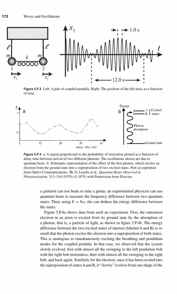
172 Waves and Oscillations
Figure 5.P.3 Left: A pair of coupled pendula. Right: The position of the left mass as a functionof time.
Figure 5.P.4 a: A signal proportional to the probability of ionization plotted as a function ofdelay time between arrival of two different photons. The oscillations shown are due toquantum beats. b: Schematic representation of the effect of the first photon, which excites anelectron from the ground state into a superposition of two excited states. Part (a) reprintedfrom Optics Communications, 31, G. Leuchs et al., Quantum Beats Observed inPhotoionization, 313–316 (1979), © 1979, with Permission from Elsevier.
a guitarist can use beats to tune a guitar, an experimental physicist can usequantum beats to measure the frequency difference between two quantumstates. Then, using E = hω, she can deduce the energy difference betweenthe states.
Figure 5.P.4a shows data from such an experiment. First, the outermostelectron in an atom is excited from its ground state by the absorption ofa photon, that is, a particle of light, as shown in figure 5.P.4b. The energydifference between the two excited states of interest (labeled A and B) is sosmall that the photon excites the electron into a superposition of both states.This is analogous to simultaneously exciting the breathing and pendulummodes for the coupled pendula. In that case, we observed that the systemslowly evolved, first with almost all the swinging in the left pendulum bobwith the right bob motionless, then with almost all the swinging in the rightbob, and back again. Similarly for the electron, once it has been excited intothe superposition of statesAand B, it “slowly” evolves from one shape of the

Chapter 5 ■ Symmetric Coupled Oscillators and Hilbert Space 173
“electron cloud” (call it shape 1) to another (call it shape 2) and then back.In this context, “slowly” means on the order of tens of ns (nanoseconds),which is indeed slow on the timescale of many atomic events.
It turns out that, when the electron cloud is in shape 1, it is easier toremove the electron entirely from the atom than it is when the electron cloudis in shape 2. In other words, the probability for ionization of the atom (byabsorption of a second photon) is higher for shape 1 than shape 2. The authorsof this paper used a pair of photon pulses to exploit this fact. A photon fromthe first pulse excites the electron into the superposition of states A and B,and a photon from the second pulse might be able to ionize the atom, if thephoton arrives when the electron cloud is in shape 1. Figure 5.P.4a showsa signal called “β4” measured by the experimenters, which is proportionalto the probability of ionization. The horizontal axis shows the time delaybetween the two photon pulses.
Using this data, deduce the energy difference between states A and B;express your answer in electron Volts (abbreviated eV), where 1 eV = 1.602× 10⁻¹⁹ J. (For comparison, the energy difference between the ground stateand state B in this atom is 3.68 eV. You should find that the energy differencebetween A and B is much smaller than this.) Note that the actual energy leveldiagram is more complex than the simplified version shown here, whichexplains why the graph above is only roughly sinusoidal.
5.8 State what is wrong with the following statement: “There is no differencebetween a normal mode and an eigenvector – the two terms are inter-changeable.” (As part of your response, provide a corrected version of thestatement.)
5.9 State what is wrong with the following paragraph: “Consider an undampedmass on a spring. When the mass is given an initial ‘kick’ (by impartingsome initial velocity), thereafter it always oscillates at ω0 = √
k/m, no matterwhether the initial kick is to the left or to the right, and no matter how hard thekick is. Now, consider an undamped symmetric coupled pendulum system.In the same way, if the left mass is given an initial kick (while the rightmass is left initially motionless, but released immediately after the kick), thesystem always oscillates at one of the normal mode frequencies, either ωpor ωb, depending on whether the initial kick is to the right or to the left.”(As part of your response, provide a corrected version of the statement.)
5.10 Two coupled identical pendula of mass 3 kg are oscillating, having started atrest with positions x1 (0) = 0.22 m and x2 (0) = −0.15 m. Mass 1 has Tfast =0.5 s (where Tfast is the period of the rapid oscillations) and Tbeat = 10 s.
(a) Find the amplitudes of the breathing and pendulum modes.(b) Find the position of mass 1 as a function of time.
5.11 Two coupled pendula are oscillating with |x(t)〉 =(
1
7√
2m
)cos [(5 rad/s) t](
11
)+
(1
3√
2m
)cos [(6.1 rad/s) t]
(1
−1
). They started from rest. What
were their initial positions?

174 Waves and Oscillations
5.12 Practice with inner products Let |A〉 =(
1.2 − 3i−2
)and |B〉 =
(6.87.1
).
(a) Evaluate 〈A | B〉 and 〈B | A〉.(b) Show that, for any two vectors |C〉 and |D〉 (which may have
complex components),〈C | D〉 = 〈D | C〉∗. In other words, showthat, to reverse the order of an inner product, you need only takethe complex conjugate of the value. (The vectors are assumed to betwo-dimensional, such as |A〉 and |B〉 are.)
(c) Find a vector that is orthogonal to |B〉, and verify the orthogonalityusing an inner product.
(d) Find a vector that points in the same direction as |B〉 but has length 1,and verify its length using an inner product.
5.13 Symmetric coupled pendula applet. Please open a browser and go to thelisting for this problem on this book’s web page. Click on the link labeled“Hilbert Space for Coupled Pendula,” and wait for the applet to load. (It maytake a couple of minutes.)Exercises (please work through all these; written responses are needed onlyas indicated by boldface):
(a) Try to set up the pendula in a pure pendulum mode (by clicking onthe Hilbert Space plot in the applet above) and then click on the‘Go!’ button. Now try a few different amplitudes.
(b) Now, set up the pendula in a pure breathing mode. Again, try a fewdifferent amplitudes.
(c) For positive breathing amplitude (downward and to the right), isthe initial position of the left pendulum bob positive or negative?How about the right one?
(d) Now set up a beat pattern so that energy is transferred back and forthbetween the two pendulum bobs periodically. First, make a perfectbeat pattern where each bob periodically comes to a complete stop,and then set up some more complicated behavior.
(e) For the beating state that you just created, look carefully at thegraphs at the bottom of the applet. Are these graphs showing thecorrect behavior of the pendulum and breathing modes? Is thebehavior of the system simply an addition of these two modes?
(f) Try pressing the button labeled “Drop Lines,” and describe whatthis is showing.
(g) Describe how the colors used in the animation help to makeconnections between the three different pictures of the applet.
(h) The angular frequency of the pendulum mode is ωp =√
g
�. The
angular frequency of the breathing mode is ωb =√
g
�+ 2k
m.
Recall what we learned about beats: A cos ω1t + A cos ω2t =2A cos ωet cos ωavt where ωav = ω1 + ω2
2and ωe = ω1 − ω2
2.

Chapter 5 ■ Symmetric Coupled Oscillators and Hilbert Space 175
Given a linear combination of these two normal modes, whatis the period and frequency of the envelope? Qualitatively, howdoes changing the spring constant (k) affect these results? Testthis hypothesis by changing k in the animation.
(i) The normal modes are mutually orthogonal – they do not influenceeach other. Why is this an illuminating way to look at a system?
(j) In order to predict the behavior of a system of coupled oscillatorsas a function of time, why is it more useful to know theamplitudes of the normal modes than the initial positions ofthe pendulum bobs?
(k) What vectors in the Hilbert space are associated with uniquefrequencies?
(l) Using the language of taking projections of vectors onto differ-ent axes, describe the process of normal mode analysis.
5.14 For a pair of symmetric pendula (or any other symmetric coupled oscillatorsystem) that is restricted to zero initial velocities, verify that the followingpeculiar-looking equation is correct:
|ep〉〈ep| + |eb〉〈eb| = 1.
Hint: Consider what happens when you apply each side of the equation toan arbitrary Hilbert space vector |A〉, that is, when you write ( |ep〉〈ep| +|eb〉〈eb| ) |A〉 = 1|A〉 . If you can explain why this equation must be true, then(because |A〉 is arbitrary), the original version of the equation must also becorrect.
5.15 Each pendulum bob in a pair of symmetric coupled pendula has mass 0.25 kg,and pendulum length 2.5 m. The bobs are connected by a spring of constant0.25 N/m. Initially, both are held immobile, with the left bob 0.25 m to theleft of its equilibrium position and the right bob at its equilibrium position.At time t = 0.25 s, they are released. Find the position of each bob as afunction of t.
5.16 A set of identical coupled pendula has ωp = 5.0 rad/s and ωb = 7.0 rad/s.The coefficients in the normal mode expansion are Cp = (0.10 m)ei(0.35) andCb = (0.15 m)ei(0.15). What is the initial position and velocity of mass 2?
5.17 For the symmetric coupled pendulum system, consider an arbitrary superpo-sition of pendulum and breathing modes, one for which the initial velocitiesare not necessarily zero. Show that, even in this superposition, the normalmode coordinates sp and sb oscillate in simple harmonic motion.
5.18 A symmetric coupled pendulum system has m = 1.5 kg, � = 0.8 m, andk = 30 N/m. At t = 0, the left bob is at a position of 5 cm, with a speed of−2 cm/s, while the right bob is at -2 cm with a speed of 3 cm/s.
(a) Show that ωp = 3.50 rad/s and that ωb = 7.23 rad/s.(b) Find |x (t)〉. Hint: after finding the real and imaginary parts of the
complex amplitudes, express the complex amplitudes in polar form,then do your taking of the real part.

176 Waves and Oscillations
5.19 A pair of symmetric coupled pendula has the following initial conditions:the left bob is at position −3.1 cm with velocity −10 cm/s, and the right bobis at position −0.2 cm with velocity 5 cm/s. Each bob has m = 1.2 kg andstring length � = 0.45 m; the spring constant is k = 2.5 N/m. At t = 5.3 s,what is the position of each bob? Show all your work clearly.
5.20 State what is wrong with the following paragraph: “Consider a symmetriccoupled pendulum system, with damping, and with a periodic drive forceapplied to the left pendulum bob, as discussed in section 5.9. When a driveforce of angular frequency ωd is applied, the steady-state motion x1 (t) ofthe left bob is always the sum of an oscillation at ωb and an oscillationat ωp. As ωd is varied, the relative amplitude of the responses at ωb andωp changes.” (As part of your response, provide a corrected version of theparagraph.)
5.21 Two lightly damped identical pendula are coupled together with a spring withspring constant 15.0 N/m. The masses of the pendula are 3.00 kg, their lengthsare 1.20 m, and the damping coefficient is b = 0.500 kg/s. The support pointSL for the left pendulum (where the string is attached to the ceiling) canbe moved left and right in a sinusoidal pattern, while the support point forthe right pendulum is held motionless. (a) At what angular frequency shouldthe support point SL be moved to produce the largest steady state responsein the coupled pendulum system? (b) Make a semi-quantitative argumentshowing that, if the system is driven at this angular frequency (by movingSL), the response of the pendulum mode is negligible, bearing in mind that thesystem is lightly damped. Hint: Calculate the FWHM of the power resonancecurve. If the drive frequency is further away from the resonance frequencythan four times the FWHM, the response will be very small indeed. (c) Forthe angular frequency you calculated in part (a), what is the ratio of theamplitude of the right pendulum to the amplitude of motion of SL?
5.22 (Please do problems 5.4 and 5.20 before beginning this exercise.)You are partof a team designing an experiment for the International Space Station. Partof the experiment involves a large box, labeled B in figure 5.P.5a. Duringthe experiment, box B will float inside the space station, in an air-filledchamber. It will be tethered by a spring to a vibrating panel, labeled P, whichis attached to the side of the space station. Panel P will oscillate left and rightat a very low frequency (0.010 Hz); these vibrations should be transmittedvia the tether to box B. However, other team members have told you thatunwanted effects will cause panel P also to oscillate with the same amplitudeat frequencies of 75.0 Hz. In other words, the motion of panel P will be
xP = Ad
(cos ωwt + cos ωut
),
where ωw = 2π (0.010 Hz) is the angular frequency of the wanted oscil-lations, ωu = 2π (75.0 Hz) is the angular frequency of the unwantedoscillations, and A = 0.05 m is the amplitude of oscillation.
Your job is to finalize the design of the tether, which must be 1.23 m long,so as to minimize the transmission of the unwanted oscillations.You are given

Chapter 5 ■ Symmetric Coupled Oscillators and Hilbert Space 177
Figure 5.P.5 Three configurations fortethering box B to panel P, which is part of
the International Space Station.
a spring which is 1.23 m long, and has a spring constant of 154 N/m. Box Bhas a mass of 54.7 kg. Tests of the air resistance of box B show that, whenit is moving at 2.00 m/s, it experiences a force from the air of 1.53 N.
(a) If you simply connect box B to panel P using the spring, as shownin figure 5.P.5a, explain why the resulting steady-state behavior ofbox B, xB (t), is simply the steady-state behavior for xP = Ad cos ωwtadded to the steady state behavior for xP = Ad cos ωut.
(b) If you now wait for a steady state to be achieved, what is the ratioof the amplitude of unwanted oscillations of box B (at 75.0 Hz) tothe amplitude of wanted oscillations of box B (at 0.010 Hz)?
You take the results of your calculations to your team leader.“Well,” she says, “that’s a pretty impressive reduction of those 75 Hzoscillations. Unfortunately, this is not good enough—the undesiredoscillations must be reduced in amplitude even further. Even moreunfortunately, it’s too late to order a different spring to use as thetether.”
Then, inspiration strikes you! You could cut the spring into twopieces, and insert an extra mass in the middle, as suggested in figure5.P.5b. This would change the resonant characteristics of the system,and so might improve rejection of the undesired oscillations. “Goodidea!” says your leader, “Crunch the numbers for me.”

178 Waves and Oscillations
You have a mass of 5.00 kg available; to simplify your calculation,assume it has a diameter which is negligible on the scale of thelength of the spring. Air resistance tests on the 5.00 kg mass showthat, when it is moving at 2.00 m/s, it experiences a force from theair of 0.33 N.
As you showed in part (b), the amplitude of oscillation of box Bat 75.0 Hz is very small in any case. Therefore, to make your lifesimpler in determining the best configuration, you should make theassumption that the amplitude of motion of box B at the unwantedfrequency (75 Hz) is essentially zero, although we will still beinterested in the forces exerted on it at this frequency.
(c) Explain qualitatively why the steady-state amplitude of oscillationsof box B at the wanted frequency of 0.010 Hz is essentially the samefor configurations a and b.
(d) Compare the force exerted on box B at 75 Hz for configurationb to that for configuration a. (You should find that the force forconfiguration b is almost 1,000 times lower!)
(e) “That’s great!” says your team leader. “But what if we take youridea even further? How about if we cut the original spring into threepieces, and add another intermediate mass?” She sketches anotherpossibility (figure 5.P.5c). At first you think, “If one mass madethe situation better, then two masses will work even better, andwould reduce the 75 Hz force exerted on box B even more!” Butthen, you begin to realize that may not be right. Making the sameassumption that box B is essentially immobile, calculate the normalmode frequencies for configuration c. Calculate the Q factor foreach of the normal modes. Then, use rough approximations to showthat, in fact the force transmitted at the unwanted frequency is alittle larger than for configuration b.

6 Asymmetric Coupled Oscillators
and the Eigenvalue Equation
Asymmetric bobsCoupled inunevendance—
Now I am enthralled.
—Marian McKenzie
6.1 Matrix math
What if we have a coupled oscillator system, similar to the coupled pendula of chapter 5,in which the two oscillators are not identical? For example, what if one of the massesis larger, or one of the pendulum strings is longer? This is a very important question formechanical systems. It also has important quantum mechanical analogs, such as theformation of molecules from two different types of atoms (e.g., the CO2 molecule).
Before we dive into the physics, it will be helpful to set up the fundamentalsof matrix math. As you have seen in chapter 5, matrices provide a powerful wayof describing coupled oscillators. For asymmetric systems, we will need moresophisticated matrix operations.
Matrix multiplication
It is easiest to explain matrix multiplication with an example:⎛⎝ A B C
D E FG H I
⎞⎠
⎛⎝ j k l
m n op q r
⎞⎠
=⎛⎝ Aj + Bm + Cp Ak + Bn + Cq Al + Bo + Cr
Dj + Em + Fp Dk + En + Fq Dl + Eo + FrGj + Hm + Ip Gk + Hn + Iq Gl + Ho + Ir
⎞⎠ .
We see that multiplying two 3 × 3 matrices creates a new 3 × 3 matrix, and that toform each entry, we multiply each of the three terms in the corresponding row of the
179

180 Waves and Oscillations
left matrix with each of the three terms in the corresponding column of the right matrix:⎛⎜⎝
A B CD E F−−−−−→G H I
⎞⎟⎠
⎛⎝
−−−−→
j k lm n op q r
⎞⎠
=⎛⎜⎝ Aj + Bm + Cp Ak + Bn + Cq Al + Bo + Cr
Dj + Em + Fp Dk + En + Fq Dl + Eo + Fr
Gj + Hm + Ip��
��Gk + Hn + Iq Gl + Ho + Ir
⎞⎟⎠ .
This means that the width (number of columns) of the left matrix must match the height(number of rows) of the right matrix. Therefore, we can multiply a three-entry columnvector by a 3 × 3 matrix:⎛
⎝ A B CD E FG H I
⎞⎠
⎛⎝ j
kl
⎞⎠ =
⎛⎝ Aj + Bk + Cl
Dj + Ek + FlGj + Hk + Il
⎞⎠ .
We see that multiplying a vector by a matrix creates a new vector, which will ordinarilyhave a different length and direction. You can think of this as the matrix acting on avector to change it into a different vector. For example, the matrix(
0 −11 0
)
acts on a vector (one with two entries, of course) to rotate it by 90◦
counterclockwise,without changing its length.
Self-test: Verify that the above matrix, when applied to the vector
(23
), works as
described.
Of course, we can also create a matrix that changes the length of any vector withoutrotating it: the matrix (
A 00 A
)changes the length of any vector by a factor A:(
A 00 A
)(ab
)=
(AaAb
)= A
(ab
).
However, most matrices, when they act on a vector, change both the length and thedirection.
The way that a matrix acts on a vector to change it into a different vector isanalogous to the way a function behaves: a function acts on a number to change it intoa different number. For example, the function y (x) = x2 can act on the number 2 tochange it into the number 22 = 4. Taking this one step further, we will soon encounter“operators.” An operator acts on a function to change it into a different function. For
example, the operatord
dxacts on the function x3 to change it into the function 3x2.

Chapter 6 ■ Asymmetric Coupled Oscillators and the Eigenvalue Equation 181
Figure 6.1.1 A view of someone (as seen from the back),with right arm extended, palm facing down. The matrix A
represents a counterclockwise (as viewed from above)rotation about the vertical axis, while the matrix B
represents a counterclockwise (as viewed from the left)rotation about the horizontal axis.
You should be aware that matrix multiplication doesn’t commute, that is, the orderof multiplication matters. For example,
(A BC D
)(e fg h
)=
(Ae + Bg Af + BhCe + Dg Cf + Dh
)
while
(e fg h
)(A BC D
)=
(Ae + Cf Be + DfAg + Ch Bg + Dh
).
Since matrices can be used to represent rotations, we can see how this lack ofcommutation works for one particular case. Stand up now (really!). Hold your right armup, so that it’s parallel to the floor, extending to the right away from your body, with yourpalm facing down, as shown in figure 6.1.1. We denote matrices using capital bold-faceletters that have hats. Let the matrix A represent a 90
◦rotation counterclockwise (as
viewed from above) about a vertical axis passing through your right shoulder (ouch!).Let the matrix B represent a 90
◦rotation counterclockwise (as viewed from someone
standing to your left) about a horizontal axis which passes through both your shoulders.Now, let the combination AB act on your arm:
AB (arm pointing right, palm down) = A [B (arm pointing to right, palm down)]= A (arm pointing right, palm pointing back)= arm pointing forward, palm pointing right
If instead you do the operations in the other order, the result is very different:
BA (arm pointing right, palm down) = B [A (arm pointing to right, palm down)]= B (arm pointing forward, palm down)= arm pointing down, palm pointing back
Determinants
The study of determinants dates back to the third century BC in China, actuallypreceding the study of matrices. The word “determinant” was coined by Gauss in1801, because they determine whether a system of equations (represented by a matrix)

182 Waves and Oscillations
has a unique solution. We will use this property to find the frequencies of the normalmodes.
The determinant of a 2 × 2 matrix is defined as follows:
det
(a bc d
)≡ ad − bc. (6.1.1)
For larger matrices, you must use a multi-step procedure. First, you put alternating +and − signs above the columns. Then, multiply the top left matrix element by the +sign you just wrote above it and by the determinant of the smaller matrix formed byignoring the top row and the left column, thus forming the first term in the determinant:
det
⎛⎜⎜⎝
+ − +a b cd e fg h i
⎞⎟⎟⎠ = +a det
(e fh i
)+ . . .
Now, move to the next entry in the top row. Multiply it by the − sign you wrote aboveit, and by the determinant of the smaller matrix formed by ignoring the top row andthe second column:
det
⎛⎜⎜⎝
+ − +a b cd e fg h i
⎞⎟⎟⎠ = +a det
(e fh i
)− b det
(d fg i
)+ . . .
Repeat this procedure, adding terms to the determinant, until you get to the rightmostentry of the top row; for our example, there is only one more term:
det
⎛⎜⎜⎝
+ − +a b cd e fg h i
⎞⎟⎟⎠ = +a det
(e fh i
)− b det
(d fg i
)+ c det
(d eg h
)
Using this procedure, you can, for example, reduce the calculation of the determinantof a 5 × 5 matrix to the calculation of the determinants of five 4 × 4 matrices. Each ofthese can in turn be reduced to the calculation of four 3 × 3 matrices. Each of these canbe reduced to the calculation of three 2 × 2 matrices, for which you can use equation(6.1.1).
In practice, for the determinants of anything larger than a 3 × 3 matrix, you mayprefer to use a symbolic algebra program, such as Mathematica. Instructions are givenon the website for this book, under the listing for this section.
6.2 Equations of motion and the eigenvalue equation
We’ll start by considering just two nonidentical oscillators, but the method we developwill be easily generalizable to a larger number. Our model system is one with twocoupled pendula, where the lengths and masses might be different, as shown infigure 6.2.1. We expect that there are normal mode solutions for this system, and

Chapter 6 ■ Asymmetric Coupled Oscillators and the Eigenvalue Equation 183
Figure 6.2.1 An asymmetric coupled pendulum system.
once we have found them, we can use the techniques of chapter 5 to perform normalmode analysis, and find the behavior of the system as a function of time, given theinitial conditions. However, it is no longer obvious exactly what the normal modesare; it appears likely that there would be some type of breathing mode, and some typeof pendulum mode, but perhaps the amplitudes for the two bobs would be different.
In Hilbert space terms, we are trying to find the two eigenvectors, that is, thetwo vectors that describe the initial positions of the bobs for the normal modes (forzero initial velocities). It will turn out that these eigenvectors are always mutuallyperpendicular, reflecting the fact that the different normal modes act as completelyindependent oscillators.1
To find the normal modes, we fall back on the procedure used in chapters 1–4:
Step 1: Apply FTotal = mx to each object in the system to get one differential equaitonfor each object.
Your turn: Show that the application of FTotal = mx to the left bob gives
x1 + ω2Ax1 − k
m1x2 = 0, (6.2.1)
where ω2A ≡ g
�1+ k
m1(6.2.2)
Concept test: Explain why ωA represents the angular frequency at which bob 1 wouldoscillate if bob 2 were held fixed at x2 = 0. (Answer below.2)
1. However, for systems of coupled oscillators with unequal masses, the axes of Hilbert space (i.e.,the x10 and x20 axes for the case of a two-oscillator system) must be scaled according to thesquare root of the corresponding mass for this orthogonality to work out correctly. There is noquantum mechanical analogy for this, so we will not spend much time on it. (The analogy wouldbe a particle whose mass depends on position.) The procedure is detailed in section 6.7.

184 Waves and Oscillations
Similarly, applying FTotal = mx to the right bob gives
x2 + ω2B x2 − k
m2x1 = 0, (6.2.3)
where ω2B ≡ g
�2+ k
m2. (6.2.4)
Step 2: Guess a solution. We believe there will be normal mode solutions, that is,solutions in which all parts of the system move with the same frequency, but may havedifferent (perhaps negative or zero) amplitudes. Also, based on our experience withthe symmetric coupled pendula, we expect that the phases of all the objects in a normalmode will be the same.3 The most general way to represent such a motion would be
x1 = Re z1 z1?= X1eiϕeiωt .
x2 = Re z2 z2?= X2eiϕeiωt .
Note that the phases and frequencies are the same for both bobs; only the amplitudesX1 and X2 are different. By the correct choice of when t = 0, we can arrange to haveϕ = 0, so that our guess simplifies to
z1?= X1eiωt z2
?= X2eiωt . (6.2.5)
With this choice of when t = 0, we see that the amplitudes have a simple interpretation:X1 = x10 and X2 = x20.
Step 3: Plug the guess into the DEQs, and see whether it works, and whether there arerestrictions on the parameters in the guess. By analogy with the symmetric coupledpendulum system, we expect that there will be restrictions on ω and on the relative
amplitudes, that is, on the ratioX2
X1. Plugging equation (6.2.5) into (6.2.1) gives
− ω2X1 eiωt + ω2AX1 eiωt − k
m1X2 eiωt = 0
⇔ ω2AX1 − k
m1X2 = ω2X1. (6.2.6a)
2. The total force on bob 1 is the pendulum force −m1g
�1x1 plus the spring force, which depends
on the relative position of the two bobs: Fspring = −k(x1 − x2
). Thus, if x2 = 0, the total
force reduces to Ftotal = −keffx1, where keff = m1g
�1+ k. Therefore, bob 1 will oscillate with
ω =√
keff
m1=
√g
�1+ k
m1.
3. “But wait!” you say, “In the breathing mode, aren’t the bobs 180◦
out of phase?” This is indeed onecorrect way of describing the breathing mode of symmetric coupled pendula: positive amplitudesfor both bobs, and 180
◦phase difference. However, it is completely equivalent to say that one
bob has a negative amplitude, and that the phase factors are the same. That’s the option we’llchoose.

Chapter 6 ■ Asymmetric Coupled Oscillators and the Eigenvalue Equation 185
Similarly, plugging into equation (6.2.3) gives
ω2BX2 − k
m2X1 = ω2X2. (6.2.6b)
We saw in chapter 5 that matrix methods were helpful. So, let us cast equations (6.2.6)into matrix form, with the top line of the matrix equation representing (6.2.6a), andthe bottom line representing (6.2.6b):
⎛⎜⎜⎝
ω2A − k
m1
− k
m2ω2
B
⎞⎟⎟⎠
(X1X2
)= ω2
(X1X2
). (6.2.7)
Your turn: Verify that the top line of equation (6.2.7) really does representequation (6.2.6a), and that the bottom line really does represent equation (6.2.6b).
Note that this equation looks similar in some ways to one encountered in section 6.1,(A 00 A
)(ab
)= A
(ab
).
However, the important difference is that when any vector
(ab
)is multiplied by the
matrix
(A 00 A
), only the length of the vector is changed (and not its direction).
In contrast, equation (6.2.7) only works for a small number of special vectors. Forexample, if we apply the matrix in equation (6.2.7) to an “arbitrary” vector such as(
10
), we get
⎛⎜⎜⎝
ω2A − k
m1
− k
m2ω2
B
⎞⎟⎟⎠
(10
)=
⎛⎜⎝ ω2
A
− k
m2
⎞⎟⎠ �= const.
(10
).
Each special vector for which equation (6.2.7) does hold represents the initial positionsX1 and X2 of the bobs in one of the normal modes. Therefore, these special vectorsare the eigenvectors, multiplied by an amplitude.
Example: in the symmetric coupled pendula, we found that the breathing mode was
represented by the eigenvector∣∣eb
⟩ = 1√2
(1
−1
). We could excite this mode with any
overall amplitude. For example, we could set x10 = 5 cm and x20 = −5 cm. Then, (makinguse of the facts that, for the symmetric case ωA = ωB and m1 = m2 = m) the left side of
continued

186 Waves and Oscillations
equation (6.2.7) would read⎛⎜⎜⎝
ω2A − k
m1
− k
m2ω2
B
⎞⎟⎟⎠
(X1X2
)=
⎛⎜⎝ ω2
A − k
m
− k
mω2
A
⎞⎟⎠
(5 cm
−5 cm
).
Let’s verify that equation (6.2.7) really holds for this case, bearing in mind that for this
symmetric case ω2A ≡ g
�+ k
m:
⎛⎜⎝ ω2
A − k
m
− k
mω2
A
⎞⎟⎠(
5 cm−5 cm
)=⎛⎜⎝ ω2
A (5 cm) − k
m(−5 cm)
− k
m(5 cm)+ω2
A (−5 cm)
⎞⎟⎠=
(ω2
A + k
m
)(5 cm
−5 cm
)
=[(
g
�+ k
m
)+ k
m
](5 cm
−5 cm
)=(
g
�+ 2k
m
)(5 cm
−5 cm
)=ω2
b
(5 cm
−5 cm
).�
As we had arranged, ω which appears in equation (6.2.7) is the normal mode frequency.
Each different eigenvector (or simple multiple thereof) which solves equation(6.2.7) is associated with a different squared normal mode angular frequency ω2. Ourjob now becomes finding the eigenvectors and corresponding “eigenvalues” ω2 forwhich equation (6.2.7) holds. This form of equation is called an “eigenvalue equation”:
(6.2.7):
⎛⎜⎜⎝
ω2A − k
m1
− k
m2ω2
B
⎞⎟⎟⎠
︸ ︷︷ ︸matrix A
(X1X2
)︸ ︷︷ ︸
eigenvector
= ω2︸︷︷︸eigenvalue
(X1X2
)︸ ︷︷ ︸
eigenvector
.
To write this in bra-ket notation, we define∣∣eu
⟩ ≡(
X1X2
), where the subscript “u”
indicates unnormalized, that is, the vector∣∣eu
⟩does not necessarily have length 1. Later,
we will discuss the (simple) process for normalizing eigenvectors. With this notation,the equation becomes:
A∣∣eu
⟩ = ω2∣∣eu
⟩.
6.3 Procedure for solving the eigenvalue equation
Matrix eigenvalue equations such as equation (6.2.7) have been studied for a long time,and there is a well-developed recipe to find the eigenvalues and eigenvectors.
Step A: Write the characteristic equationThe “characteristic equation” is the same as the eigenvalue equation, just
rearranged so that the right side is zero.

Chapter 6 ■ Asymmetric Coupled Oscillators and the Eigenvalue Equation 187
Your turn: Show that the eigenvalue equation
(6.2.7):
⎛⎜⎜⎝
ω2A − k
m1
− k
m2ω2
B
⎞⎟⎟⎠
(X1X2
)= ω2
(X1X2
)
eigenvalue equation for two coupled oscillators
is equivalent to ⎛⎜⎜⎝
ω2A − ω2 − k
m1
− k
m2ω2
B − ω2
⎞⎟⎟⎠
︸ ︷︷ ︸B
(X1X2
)︸ ︷︷ ︸
|eu〉
= 0. (6.3.1)
characteristic equation for two coupled oscillators
(Here, the “0” on the right side is shorthand for
(00
).) Hint: Remember that each matrix
equation is shorthand for two regular equations. If you can show that this pair of regularequations for (6.3.1) is equivalent to the pair for (6.2.7), then you’ve shown that the matrixequation (6.3.1) is equivalent to the matrix equation (6.2.7).
Step B: Use theorem from linear algebraThere is a general theorem that states that any equation of the form of
equation (6.3.1), that is, of the form B r = 0, can hold if and only if det B = 0.Proof for 2 × 2 case:
(a bc d
)︸ ︷︷ ︸
B
(ef
)= 0 ⇒
Top line : ae + bf = 0 ⇔ e = −bf
aBottom line : ce + df = 0
⎫⎬⎭ ⇒ c
(−bf
a
)+ df = 0 ⇔
−cb + ad = 0 ⇔ det B = 0�
Applying this theorem to equation (6.3.1) gives us a quadratic equation for ω2:
B r = 0 ⇒ det B = 0, that is,
.(ω2
A − ω2) (
ω2B − ω2
)− k2
m1m2= 0 ⇔
ω4 − ω2(ω2
A + ω2B
)+
(ω2
Aω2B − k2
m1m2
)= 0.

188 Waves and Oscillations
Using the quadratic equation for the variable ω2 , we obtain
ω2 =ω2
A + ω2B ±
√(ω2
A + ω2B
)2 − 4
(ω2
Aω2B − k2
m1m2
)2
=ω2
A + ω2B ±
√(ω2
A
)2 + 2ω2Aω2
B + (ω2
B
)2 − 4ω2Aω2
B + 4k2
m1m2
2
=ω2
A + ω2B ±
√(ω2
A
)2 − 2ω2Aω2
B + (ω2
B
)2 + 4k2
m1m2
2
⇒ ω2 =ω2
A + ω2B ±
√(ω2
A − ω2B
)2 + 4k2
m1m2
2(6.3.2)
eigenvalues for two coupled oscillators
Note that this equation tells us both values of ω (i.e., the angular frequencies of bothnormal modes) because of the “±.”
Often, this is as far as we need to go, since often we only care about the frequenciesof the normal modes. However, sometimes we also wish to know the way in which themasses are moving, which means we need to find the eigenvectors. (Again, for a purenormal mode state, the eigenvectors tell us the relative initial positions of each mass,and each mass oscillates in simple harmonic motion, with amplitude equal to its initialposition.)
Step C: To find the eigenvectors, take the eigenvalues, one at a time, and substitutethem into the characteristic equation. Solve for X2 in terms of X1.
Note that we cannot find the actual values of both X1 and X2, but only theirrelative values, since we are only making use of the underlying interactions of thesystem, and not of the initial conditions; each normal mode can be excited with anarbitrary amplitude, as determined by the initial conditions. Implementing step C forthe general case, even for a system of only two coupled oscillators, is very messy andnot very instructive. Instead, we will illustrate with a special case.
Core example: Consider the special case of coupled pendula with equal masses m1 =m2 = m = 1 kg , but unequal lengths �1 = 4.33 m and �2 = 2.30 m, and let k = √
3 N/m.This is shown in figure 6.3.1. Then,
k2
m2 = 3 rad4/s4,
and ω2A ≡ g
�1+ k
m1= (2.26 + √
3) rad2/s2 = 4 rad2/s2,

Chapter 6 ■ Asymmetric Coupled Oscillators and the Eigenvalue Equation 189
Figure 6.3.1 An example of an asymmetric coupled pendulum system with equalmasses.
while ω2B ≡ g
�2+ k
m2= (4.26 + √
3) rad2/s2 = 6 rad2/s2.
Plugging these into equation (6.3.2) gives
ω2 = 4 + 6 ±√
(4 − 6)2 + 4 · 32
rad2/s2
= 10 ± √4 + 12
2rad2/s2 =
{73
rad2/s2 ⇒ ω ={√
7√3
rad/s.
We anticipate that the higher value of ω corresponds to a breathing-type mode, and thelower value to a pendulum type mode. Now, to find the eigenvectors. For the breathingmode, substitute ω2 = 7 rad2/s2 into the characteristic equation (6.3.1):⎛
⎜⎜⎝ω2
A − ω2 − k
m1
− k
m2ω2
B − ω2
⎞⎟⎟⎠
(X1X2
)= 0 ⇒
(4 − 7 −√
3−√
3 6 − 7
)rad2/s2
(X1X2
)= 0.
We now divide both sides by 1 rad2/s2, giving(4 − 7 −√
3−√
3 6 − 7
)(X1X2
)= 0 ⇒ Top line: − 3X1 − √
3 X2 = 0 ⇔ X2 = − √3 X1
Note: the bottom line of the above matrix equation tells us the same thing:
Bottom line: − √3 X1 − X2 = 0 ⇔ X2 = −√
3X1.
This redundancy arises because we cannot specify the actual values of X1 and X2, butonly their relative values, since we are only making use of the underlying interactionsof the system, and not of the initial conditions. As expected for a breathing-type mode,the amplitude for right bob, X2 is opposite in sign to that for the left bob. We also
continued

190 Waves and Oscillations
see that the amplitude for the right bob (the one with the shorter string) is larger in thismode. Expressing our result in column matrix form, we have found that the eigenvector
for the breathing mode (not yet normalized) is∣∣eub
⟩ =(
1−√
3
). This is illustrated in
figure 6.3.2a.
Figure 6.3.2 Normal modes for the system shown in figure 6.3.1. a: breathing mode.b: pendulum mode.
Your turn: Find the eigenvector for the pendulum mode by substituting ω2 = 3 rad2/s2
into the characteristic equation, (6.3.1), and then using the top line of the resulting
matrix equation to show that X2 = 1√3
X1. Now, show that the bottom line of the matrix
equation says the same thing.As expected for the pendulum mode, the amplitudes have the same sign for both
bobs, but now the right bob has a smaller amplitude, as shown in figure 6.3.2b. Expressingour result in column matrix form, we have found that the eigenvector for the pendulum
mode (not yet normalized) is∣∣∣eup
⟩=
(1
1/√
3
).

Chapter 6 ■ Asymmetric Coupled Oscillators and the Eigenvalue Equation 191
6.4 Systems with more than two objects
To generalize these ideas to a larger system of coupled oscillators, we use exactly thesame methods.4 Assuming there are N objects in the system, here is the procedure:
1. Write FTOT = mx for each object. This creates a system of N coupleddifferential equations.
2. Guess a normal mode solution, that is, guess that the position of object j isgiven by
xj?= Re
[Xj eiωt
],
where ω is the angular frequency of the normal mode, and Xj is the amplitude ofoscillation of object j . As before, we have chosen the time when t ≡ 0 so that theoverall phase factor ϕ = 0. Therefore, the amplitude Xj of object j is equal to the initialposition xj0 of object j.
3. Plug the guess back into the system of differential equations. All the terms willcontain the eiωt factor, so this can be cancelled out, leaving a system of N coupledlinear equations involving the variables Xj.
4. Write the system of equations as an eigenvalue equation, that is, a matrixequation of the form
A∣∣eu
⟩ = ω2∣∣eu
⟩,
where A is an N × N matrix, and∣∣eu
⟩is the column vector
⎛⎜⎝
X1X2...
⎞⎟⎠.
5. Rearrange the eigenvalue equation to form the characteristic equation, that is,the equivalent equation which has the form
B∣∣eu
⟩ = 0.
6. To find the eigenvalues ω2, set
det B = 0
This will give an N th-order equation for ω2, with N solutions.
4. The ideas described here work just as well for any system with more than two “degrees offreedom,” whether there are one, two, or more objects. Here, a “degree of freedom” is a wayin which the system can move that is completely independent of other degrees of freedom, atleast before the coupling between degrees of freedom is added. For example, a rigid object inthree-dimensional space has six degrees of freedom, since it can move in three directions, androtate about three axes. As another example, if we had two particles, each of which was keptnear a particular point in three-dimensional space by restoring forces, and these particles werecoupled together by a spring, that would be a system with six degrees of freedom. In our maindiscussion, however, we’ll stick to particles that are constrained to move in only one dimension,since this is easier to illustrate and conceptually simpler.

192 Waves and Oscillations
7. To find the eigenvectors, take each value of ω2, one at a time, and substitute itback into the characteristic equation. Solve for X2, X3 , etc., in terms of X1.
This procedure is guaranteed to work. (For systems of five or more objects, it willnot usually be possible to solve for the eigenvalues analytically, but they can alwaysbe found by numerical approximation.) This is a tremendously important realization,since we have just proved that, for a system of N objects, we will always be able to findN normal modes. In principle, we could write a system of N uncoupled differentialequations to represent these modes. (This is seldom necessary, but we certainly coulddo it.) This system of DEQs would represent the behavior of the system just as well asthe system of N DEQs which describes the positions of the N objects. Therefore, wecan quite generally conclude:
For a one-dimensional system, the number of normal modes is equal to the
number of masses. Therefore, giving the amplitudes and phases of all the
normal modes provides just as complete a description of the system as giving
x(t) for each object in the system.
We will do a fairly generic example of a one-dimensional system with three objects,from which it will be obvious how to generalize to a one-dimensional system with anynumber of objects. Consider the system shown in figure 6.4.1. Masses 1 and 3 areconnected by the long spring k13.
1. Applying FTOT = mx to m1 gives
−k1x1 − m1g
�x1 − k12
(x1 − x2
) − k13
(x1 − x3
) = m1x1. (6.4.1)
This is the real part of
−k1z1 − m1g
�z1 − k12
(z1 − z2
) − k13
(z1 − z3
) = m1z1. (6.4.2)
(We won’t bother to apply FTOT = mx to the other masses, since the pattern willbecome obvious just from m1.)
Figure 6.4.1 system of three coupledpendula with all possible couplings.
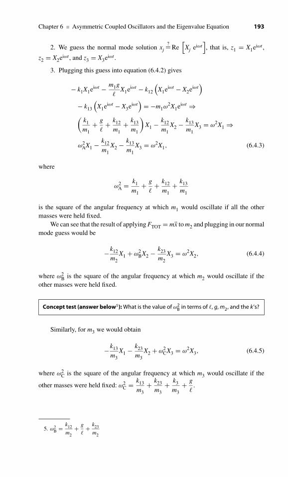
Chapter 6 ■ Asymmetric Coupled Oscillators and the Eigenvalue Equation 193
2. We guess the normal mode solution xj?= Re
[Xj eiωt
], that is, z1 = X1eiωt ,
z2 = X2eiωt , and z3 = X3eiωt .
3. Plugging this guess into equation (6.4.2) gives
− k1X1eiωt − m1g
�X1eiωt − k12
(X1eiωt − X2eiωt
)− k13
(X1eiωt − X3eiωt
)= −m1ω
2X1eiωt ⇒(k1
m1+ g
�+ k12
m1+ k13
m1
)X1 − k12
m1X2 − k13
m1X3 = ω2X1 ⇒
ω2AX1 − k12
m1X2 − k13
m1X3 = ω2X1, (6.4.3)
where
ω2A = k1
m1+ g
�+ k12
m1+ k13
m1
is the square of the angular frequency at which m1 would oscillate if all the othermasses were held fixed.
We can see that the result of applying FTOT = mx to m2 and plugging in our normalmode guess would be
−k12
m2X1 + ω2
BX2 − k23
m2X3 = ω2X2, (6.4.4)
where ω2B is the square of the angular frequency at which m2 would oscillate if the
other masses were held fixed.
Concept test (answer below5): What is the value of ω2B in terms of �, g, m2, and the k’s?
Similarly, for m3 we would obtain
−k13
m3X1 − k23
m3X2 + ω2
CX3 = ω2X3, (6.4.5)
where ω2C is the square of the angular frequency at which m3 would oscillate if the
other masses were held fixed: ω2C = k13
m3+ k23
m3+ k3
m3+ g
�.
5. ω2B = k12
m2+ g
�+ k23
m2

194 Waves and Oscillations
4. We can write equations (6.4.3), (6.4.4), and (6.4.5) in matrix form:
⎛⎜⎜⎜⎜⎜⎜⎝
ω2A −k12
m1−k13
m1
−k12
m2ω2
B −k23
m2
−k13
m3−k23
m3ω2
C
⎞⎟⎟⎟⎟⎟⎟⎠
⎛⎝X1
X2X3
⎞⎠ = ω2
⎛⎝X1
X2X3
⎞⎠ . (6.4.6)
In fact, now that we’ve gone through this procedure, you can probably construct theequivalent of equation (6.4.6) for whatever system is given just by inspection.
From here, we could in principle go on to steps 5, 6, and 7 to find the eigenvaluesand eigenvectors. However, it is much easier to do this using a symbolic algebraprogram (such as Mathematica), especially if there are more than three objects. Explicitinstructions for how to do this, including an example, are given on the website for thistext under the listing for this section.
6.5 Normal mode analysis for multi-object, asymmetrical systems
Our treatment of normal mode analysis in section 5.8 depended only on theorthonormality of the normalized eigenvectors, so we can use exactly the samemethods for asymmetric systems with many objects, as long as we use the normalizedeigenvectors. We will go over things again below, to make sure this is clear. However,first we need to understand the process for normalizing eigenvectors.
How to normalize eigenvectors
If we find a vector∣∣eu
⟩which solves the eigenvalue equation A
∣∣eu
⟩ = ω2∣∣eu
⟩, then the
vector D∣∣eu
⟩(where D is a constant, perhaps a complex constant) will also solve the
equation, since
A∣∣eu
⟩ = ω2∣∣eu
⟩ ⇔ DA∣∣eu
⟩ = D ω2∣∣eu
⟩ ⇔ A(D∣∣eu
⟩) = ω2 (D ∣∣eu
⟩).
Thus, there are an infinite number of vectors, all pointing along the same direction inHilbert space but with different lengths, which solve the eigenvector equation for aparticular eigenvalue ω2. However, there is one vector that is particularly helpful: thenormalized eigenvector, that is, the vector that has length 1 in this direction. (Again,just 1, not 1 m.)
Core example:
For the example from the end of section 6.3, we found that the eigenvector for
the breathing mode is of the form∣∣eub
⟩ =(
1−√
3
). To normalize it, we just divide by the

Chapter 6 ■ Asymmetric Coupled Oscillators and the Eigenvalue Equation 195
length: Length =√
12 +(−√
3)2 = 2. So, the normalized eigenvector is
∣∣eb
⟩ =∣∣eub
⟩Length
=⎛⎝ 1
2
−√
32
⎞⎠ .
As a check, if we’ve correctly normalized it we should have⟨eb|eb
⟩ = 1:
(12
−√
32
)⎛⎝ 1
2
−√
32
⎞⎠ = 1
4+ 3
4= 1�
The above normalization procedure is only valid when the masses are equal; themore general procedure is treated in section 6.7.
Normal mode analysis
Here, I convince you that we only need a complete orthonormal basis in order to usethe same formulas for normal mode analysis as we derived in section 5.8. Let
∣∣e1
⟩be
the normalized eigenvector for mode n = 1, and∣∣e2
⟩be the normalized eigenvector for
mode n = 2, and so on. Be careful not to confuse the mode index n with the mass index j.
For example,∣∣e1
⟩ =⎛⎜⎝
X1X2...
⎞⎟⎠ is a vector of length 1 specifying the initial positions of
the masses (with zero initial velocities) for normal mode n = 1. The subscript “1” in∣∣e1
⟩refers to mode number 1, whereas the subscript “1” in X1 refers to mass number
1. It is easy to tell which type of index is being used from the context: any subscripton a vector (e.g.,
∣∣e1
⟩) or a frequency (e.g., ω1) is a mode index. We will consistently
use the symbol n or m for the mode index and the symbol j for the mass index.As detailed earlier, giving the amplitudes and phases of all the normal modes
provides just as complete a description of the system as giving x(t) for each object in
the system. This means that, for any state of the system, the vector |x (t)〉 =⎛⎜⎝
x1 (t)x2 (t)
...
⎞⎟⎠
can be written as a superposition of the normal modes, that is,
|x (t)〉 = Re
[N∑
n=1
Cneiωn t∣∣en
⟩](6.5.1)
(Again, the∣∣en
⟩’s (i.e.,
∣∣e1
⟩,∣∣e2
⟩, etc.) are the normalized eigenvectors representing the
different normal modes.)This is the more general version of the normal mode expansion
for two coupled oscillators, (5.8.1): |x (t)〉 = Re[Cpeiωpt
∣∣∣ep
⟩+ Cbeiωbt
∣∣eb
⟩].
To find the complex amplitudes Cn in the normal mode expansion (6.5.1) fromthe initial positions and velocities of the masses, we follow the example of section 5.8.

196 Waves and Oscillations
According to equation (6.5.1), the initial positions of the objects are given by6
∣∣x0
⟩ ≡⎛⎜⎝
x10x20...
⎞⎟⎠ = Re
[N∑
n=1
Cn
∣∣en
⟩], (6.5.2)
and the initial velocities are given by
∣∣x0
⟩ ≡⎛⎜⎝
x10x20
...
⎞⎟⎠ = d
dt[|x (t)〉]t=0 = d
dt
[Re
[N∑
n=1
Cneiωnt∣∣en
⟩]]t=0
= Re
[N∑
n=1
iωnCn
∣∣en
⟩]. (6.5.3)
Next, we write the complex amplitudes in Cartesian form:
Cn = Re Cn + i Im Cn.
This allows us to rewrite equations (6.5.2) and (6.5.3):
∣∣x0
⟩ = Re
[N∑
n=1
Cn
∣∣en
⟩] =N∑
n=1
Re(Cn
) ∣∣en
⟩, (6.5.4)
(since the∣∣en
⟩’s are real) and
∣∣x0
⟩ = Re
[N∑
n=1
iωnCn
∣∣en
⟩] = Re
[N∑
n=1
iωn
(Re Cn + i Im Cn
) ∣∣en
⟩]
Re
[N∑
n=1
ωn
(iRe Cn − Im Cn
) ∣∣en
⟩] = −N∑
n=1
ωn Im(Cn
) ∣∣en
⟩. (6.5.5)
For the remainder of this section, we assume the masses of coupled oscillatorsare equal. This is the case of most interest, because it is most closely analogous withquantum mechanics. The general case of nonequal masses is treated in section 6.7.
Next, we need a couple of results regarding the normalized eigenvectors. Thenormal modes do not interact with each other, therefore the eigenvectors are mutuallyorthogonal, that is, ⟨
em|en
⟩ = 0 if n �= m
(We prove this more rigorously in section 6.7.) The eigenvectors∣∣en
⟩are normalized,
that is, ⟨en|en
⟩ = 1
6. Note that here, we use the subscript “0” to indicate t = 0. It does not indicate n = 0. (In fact,there is no mode n = 0, since we start numbering the modes at n = 1.)

Chapter 6 ■ Asymmetric Coupled Oscillators and the Eigenvalue Equation 197
We can summarize the above two equations by writing⟨em|en
⟩ = δmn, (6.5.6)
where the “Kronecker delta function” (pronounced “Crow-neck-er”) is defined by
δmn ≡{
1 if n = m0 if n �= m
(6.5.7)
Now, following the lead of section 5.8, we try taking the inner product of∣∣x0
⟩with
each of the normalized eigenvectors:
⟨em|x0
⟩ = ⟨em
∣∣ ( N∑n=1
Re(Cn
) ∣∣en
⟩) =N∑
n=1
Re(Cn
) ⟨em|en
⟩.
(Note that we must use⟨em
∣∣ in the left side of the inner product above, rather than⟨en
∣∣,because the subscript n is already being used in the summation on the right side of theinner product.) Because of orthonormality (as expressed in equation (6.5.6)), all theterms in the sum are zero, except the one for which m = n, and for that term we have⟨em=n|en
⟩ = 1. Therefore, ⟨em|x0
⟩ = Re(Cm
).
Since we have eliminated the sum over n, we could just as well write this as⟨en|x0
⟩ =Re
(Cn
)⇒ Re
(Cn
) = ⟨en|x0
⟩, (6.5.8a)
which is the generalized version of equation (5.8.2a): Re(
Cp
)=
⟨ep|x0
⟩.
Next, again following the lead of section 5.8, we try taking the inner product of∣∣x0
⟩with each of the normalized eigenvectors:
⟨em|x0
⟩= ⟨em
∣∣(−N∑
n=1
ωnIm(Cn
)∣∣en
⟩)=−N∑
n=1
ωnIm(Cn
)⟨em|en
⟩=−ωmIm(Cm
).
Again, since the sum over n has been eliminated, we could write this as⟨en|x0
⟩ = −ωnIm
(Cn
)⇒ Im
(Cn
) = − 1
ωn
⟨en|x0
⟩, (6.5.8b)
which is the generalized version of equation (5.8.2b): Im(
Cp
)= − 1
ωp
⟨ep|x0
⟩.
Note that for the important special case of∣∣x0
⟩ = 0, Im(Cn
) = 0, so that theamplitudes that appear in the normal mode expansion (6.5.1) reduce to Cn =Re
(Cn
) =⟨en|x0
⟩.
Stated in graphical terms, this means that, in the normal mode expansion for thespecial case
∣∣x0
⟩ = 0, the coefficient along the Hilbert space axis corresponding tomode n is given by the inner product of the initial state of the system
∣∣x0
⟩with the

198 Waves and Oscillations
normalized eigenvector for that mode,∣∣en
⟩. Just as for the coupled pendulum, this idea
of taking inner products to find the “projections” of the state of the system along thenormal mode “directions” in Hilbert space (by taking these inner products) is exactlyanalogous to the process of finding the projections of an ordinary vector along thex- or y-axis (by taking dot products with i or j).
6.6 More matrix math
In this section, we go over a few additional aspects of matrix math that are needed forsection 6.7, and that are also quite important for the study of quantum mechanics.
Inverse matrices and the identity matrix
One can show that, if and only if the determinant of a matrix A doesn’t equal zero,then one can find the inverse matrix A−1, such that
AA−1 = A−1A = I,
where I is the identity matrix:
I =⎛⎜⎝
1 0 · · ·0 1 0... 0
. . .
⎞⎟⎠ .
Note that multiplying by I has no effect on anything, just as multiplying by 1. Forexample, in multiplication of 2 × 2 matrices, we have
IA =(
1 00 1
) (a bc d
)=
(a bc d
).
This means that the matrix A−1 “undoes” the effect of the matrix A. For instance, ifthe matrix A rotates vectors by 31
◦clockwise about the z-axis, then the matrix A−1
rotates vectors by 31◦
counterclockwise about the z-axis.
Another feature of bra-ket notation
We’ve discussed how, unlike multiplication of numbers, the order matters for matrixmultiplication. However, matrix multiplication is associative, meaning, for example,that
A(
BC)
=(
AB)
C.
We can take advantage of this in bra-ket notation. Let’s define an arbitrary bra 〈g| =(g1 g2
), an arbitrary ket |x〉 =
(x1x2
), and an arbitrary matrix A =
(a bc d
). Then,
we can write
〈g| A |x〉 .

Chapter 6 ■ Asymmetric Coupled Oscillators and the Eigenvalue Equation 199
One might think that this is ambiguous. Should we interpret this as(〈g| A
)|x〉, meaning
first do the matrix multiplication 〈g| A, then matrix multiply the result by |x〉? Or,
should we instead interpret it as 〈g|(
A |x〉)
? However, because matrix multiplication is
associative, these two interpretations give the same result. (You can show this explicitlyin problem 6.16.) So, when interpreting 〈g| A |x〉, we can think of A “operating” to theleft on 〈g| or operating to right on |x〉.
Hermitian matrices
In the next section, and frequently in the study of quantum mechanics, you’ll need totake the adjoint of A |x〉: [
A |x〉]† =?
By considering a system of two masses, we’ll be able to see the general pattern. Let
|x〉 =(
x1x2
)and A =
(a bc d
).
Then,
A |x〉 =(
a bc d
) (x1x2
)=
(ax1 + bx2cx1 + dx2
).
To take the adjoint, we change it from a column matrix to a row matrix, and take thecomplex conjugate of the entries:[
A |x〉]† = (
a∗x∗1 + b∗x∗
2 c∗x∗1 + d∗x∗
2
).
Claim: We can write this as [A |x〉
]† = 〈x| A†,
where A† is the adjoint of A, that is, the matrix formed by interchanging columns (thefirst row becomes the first column, etc.) and then taking the complex conjugate of theentries.
Check:
A† =(
a∗ c∗b∗ d∗
)⇒ 〈x| A† = (
x∗1 x∗
2
)( a∗ c∗b∗ d∗
)
= (a∗ x∗
1 + b∗ x∗2 c∗ x∗
1 + d∗ x∗2
)�
Most of the matrices in the next section, and virtually all the matrices of interestin quantum mechanics, have the special property that they are “self adjoint,” meaningthat
A† = A.
We will use the more common term “Hermitian” for such matrices, instead of “selfadjoint.”

200 Waves and Oscillations
Concept test (answer below7): Which of the following matrices are Hermitian?
(a)
⎛⎜⎜⎝
ω2A − k
m1
− k
m2ω2
B
⎞⎟⎟⎠ (b)
(Ai 00 A
)(c)
(−3 −√
3−√
3 −1
)rad2/s2
In fact, we can see that any 2 × 2 Hermitian matrix can be written as
A =(
a bb∗ c
). (6.6.1)
Form of a 2 × 2 Hermitian matrix, with a and c real.
For Hermitian matrices, we have[A |x〉
]† = 〈x| A† = 〈x| A. (6.6.2)
Adjoint of products of Hermitian matrices.
In the next chapter section (and in quantum mechanics), we will need to take the adjoint
of AB |x〉, where A and B are both Hermitian. We will show that[AB |x〉
]† = 〈x| BA.
To begin, we define
|β〉 ≡ B |x〉 .
so that [AB |x〉
]† =[A |β〉
]†.
Using equation (6.6.2), this means that[AB |x〉
]† = 〈β| A. (6.6.3)
Since B is Hermitian, we have that
〈β| ≡[B |x〉
]† = 〈x| B† = 〈x| B.
Plugging this into equation (6.6.3) gives[AB |x〉
]† = 〈x| BA. (6.6.4)
True if A and B are Hermitian.
We see that, when taking the adjoint, we must reverse the order of the two matrices.
Therefore,[AB
]† = BA. Since this is not necessarily equal to AB, we see that the
product of two Hermitian matrices need not be Hermitian.
7. Only (c) is Hermitian. However, (a) would be Hermitian if m1 = m2.

Chapter 6 ■ Asymmetric Coupled Oscillators and the Eigenvalue Equation 201
6.7 Orthogonality of normal modes, normal mode coordinates,degeneracy, and scaling of Hilbert space for unequal masses
For the symmetric coupled pendulum system, we saw in chapter 5 that the quantity sp ≡1√2
(x1 + x2
), which characterizes the motion of the pendulum mode, always oscillates
at ωp, even when the system is in a superposition of pendulum and breathing modes,
and that the quantity sb ≡ 1√2
(x1 − x2
), which characterizes the breathing mode,
always oscillates at ωb. The quantities sp and sb are called “normal mode coordinates”;each is the special linear combination of the coordinates of the masses that oscillatesat the normal mode angular frequency.
Later in the chapter, we found the eigenvectors for these modes,∣∣∣ep
⟩= 1√
2
(11
)
and∣∣eb
⟩ = 1√2
(1
−1
). Therefore, defining |x (t)〉 ≡
(x1 (t)x2 (t)
), we can write
sp = ⟨ep|x (t)
⟩and sb = ⟨
eb|x (t)⟩.
We will show in this section8 that, for the case of equal masses, the analogousexpressions for normal mode coordinates hold even for asymmetrical systems withmany masses, that is, that the coordinate
sn ≡ ⟨en|x (t)
⟩, (6.7.1)
where∣∣en
⟩is one of the eigenvectors of the system, oscillates at the associated angular
frequency ωn. (As for the symmetric coupled pendulum system discussed in chapter5, the coordinate sn is associated with an sn0 axis in Hilbert space, and the direction ofthis axis is defined by
∣∣en
⟩.)
When the masses are unequal, we must modify the recipe for finding normal modecoordinates. We will show that the normal mode coordinate for unequal masses is
sn ≡ ⟨en
∣∣ M |x (t)〉 , (6.7.2)
Normal mode coordinate for the case of unequal masses.
where the “mass matrix” is M =⎛⎜⎝
m1 0 · · ·0 m2 0... 0
. . .
⎞⎟⎠ and |x (t)〉 ≡
⎛⎜⎝
x1(t)x2 (t)
...
⎞⎟⎠. Note
that M is Hermitian. Also, when all the masses equal m, equation (6.7.2) becomesxn ≡ m
⟨en|x (t)
⟩; this is the same as equation (6.7.1) except for the constant m, which
only affects the overall scaling of the normal mode coordinate.Now, we must show that equation (6.7.2) is indeed the correct definition for the
normal mode coordinate in the general case, meaning that sn oscillates at frequency
8. Most of this presentation is based on that in The Physics of Waves, by Howard Georgi(Prentice-Hall, Englewood Cliffs, NJ, 1993), pp. 81–2.

202 Waves and Oscillations
Figure 6.7.1 The same system of threecoupled pendula as shown in figure 6.4.1.
ωn, so that
sn ∝ cos(ωnt + ϕn
). (6.7.3)
To show this, we need only prove that
sn = −ω2nsn. (6.7.4)
We consider the three-mass system shown in figure 6.4.1, reproduced here forconvenience as figure 6.7.1. (It will be clear how to extend the arguments to a systemwith any number of masses.) Recall that the result of applying FTOT = mx to mass 1was (6.4.1):
−k1x1 − m1g
�x1 − k12
(x1 − x2
) − k13
(x1 − x3
) = m1x1 ⇒
− (k11 + k12 + k13
)x1 + k12x2 + k13x3 = m1x1,
where k11 is the total spring constant associated with restoring forces that act on m1but are not associated with coupling to m2 or m3. In the example of figure 6.4.1,k11 = k1 + m1g/�. We could also write the above as
−kAx1 + k12x2 + k13x3 = m1x1, (6.7.5a)
where kA = m1ω2A = k11 + k12 + k13. Applying FTOT = mx to m2 and to m3 would
similarly result in
k12x1 − kBx2 + k23x3 = m2x2 (6.7.5b)
and
k13x1 + k23x2 − kCx3 = m3x3, (6.7.5c)
where kB = m1 ω2B = k12 + k22 + k23, and k22 = m2g/� is the total spring constant
associated with restoring forces that act on m2, but are not associated with coupling tom1 or m2. (The constant kC is defined analogously to kA.)
Your turn: Show that we can then rewrite equations (6.7.5) as
−K |x (t)〉 = Md2
dt2 |x (t)〉 , (6.7.6)

Chapter 6 ■ Asymmetric Coupled Oscillators and the Eigenvalue Equation 203
where
K =⎛⎜⎝ kA −k12 −k13
−k12 kB −k23−k13 −k23 kC
⎞⎟⎠ ,
and is Hermitian.
Taking the inner product of both sides of equation (6.7.6) with∣∣en
⟩gives
−⟨en
∣∣K∣∣x(t)⟩ = ⟨en
∣∣M d2
dt2
∣∣x(t)⟩.Since neither
⟨en
∣∣ nor M has any time dependence, we can rearrange the right side,giving
−⟨en
∣∣K∣∣x(t)⟩ = d2
dt2
⟨en
∣∣M∣∣x(t)⟩,Recall that our proposed sn is given by equation (6.7.2): sn ≡ ⟨
en
∣∣M∣∣x(t)⟩. Therefore,the above gives
sn = −⟨en
∣∣K∣∣x(t)⟩.Comparing this with what we need to prove, (6.7.4): sn = −ω2
nsn, we see that wemust show ⟨
en
∣∣K∣∣x(t)⟩ = ω2nsn. (6.7.7)
The eigenvalue equation for this system is (6.4.6):⎛⎜⎜⎜⎜⎜⎜⎝
ω2A −k12
m1−k13
m1
−k12
m2ω2
B −k23
m2
−k13
m3−k23
m3ω2
C
⎞⎟⎟⎟⎟⎟⎟⎠
⎛⎝X1
X2X3
⎞⎠ = ω2
⎛⎝X1
X2X3
⎞⎠ .
We could rewrite this as
A∣∣en
⟩ = ω2n
∣∣en
⟩, (6.7.8)
where
A =
⎛⎜⎜⎜⎜⎜⎜⎝
ω2A −k12
m1−k13
m1
−k12
m2ω2
B −k23
m2
−k13
m3−k23
m3ω2
C
⎞⎟⎟⎟⎟⎟⎟⎠ .
It will be helpful to separate out the part involving the masses:
A = M−1 K, (6.7.9)

204 Waves and Oscillations
where
M−1 =
⎛⎜⎜⎜⎜⎜⎜⎝
1
m10 0
01
m20
0 01
m3
⎞⎟⎟⎟⎟⎟⎟⎠ ,
and is Hermitian.
Your turn: Do the matrix multiplication to verify that A = M−1 K.
Therefore, we can rewrite equation (6.7.8) as
M−1K∣∣en
⟩ = ω2n
∣∣en
⟩.
The adjoint of this equation is [M−1K
∣∣en
⟩]† = ω2n
⟨en
∣∣.Since both M−1 and K are Hermitian, we can apply equation (6.6.4):
[AB
∣∣x⟩]† =⟨x∣∣BA, giving ⟨
en
∣∣KM−1 = ω2n
⟨en
∣∣.Taking the inner product with M
∣∣x(t)⟩
gives⟨en
∣∣KM−1M∣∣x(t)
⟩ = ω2n
⟨en
∣∣M∣∣x(t)⟩.
The right side of this includes sn ≡ ⟨en
∣∣M∣∣x(t)⟩, so we can rewrite the above as⟨
en
∣∣KM−1M∣∣x(t)
⟩ = ω2n sn
Note that MM−1 = M−1M = I. Therefore,⟨en
∣∣KM−1M∣∣x(t)
⟩ = ⟨en
∣∣K∣∣x(t)⟩ ⇒ ⟨
en
∣∣K∣∣x(t)⟩ = ω2
nsn,
which is (6.7.7), completing the proof that sn, as defined by equation (6.7.2): sn ≡⟨en
∣∣M∣∣x(t)⟩, is indeed the normal mode coordinate.
Let us be clear about the interpretation of sn ≡ ⟨en
∣∣M∣∣x(t)⟩. This does not mean
that, in order to excite normal mode number 1, we must position the masses in an initialpattern of positions proportional to M
∣∣e1
⟩. Rather, as usual, we should position them in
a pattern proportional to∣∣e1
⟩; when they are then released, the system will be in a pure
mode 1 oscillation. However, if we instead excite the system into a superposition ofmodes, then (assuming unequal masses) the coordinate that displays a simple sinusoidalmotion at angular frequency ω1 is s1 ≡ ⟨
e1
∣∣M∣∣x(t)⟩. Other coordinates, such as
⟨e1|x(t)
⟩,
do not show simple sinusoidal motion when the system is in a superposition. (Theydo show simple sinusoidal motion when the system is in a pure mode, as do allcoordinates.)

Chapter 6 ■ Asymmetric Coupled Oscillators and the Eigenvalue Equation 205
Figure 6.7.2 Top: Coupled pendula withunequal masses. For the example discussed in thetext, m1 = 1 kg, m2 = 2 kg, � = 1 m, k = 1 N/m,
and g = 10 m/s2. Bottom: Position versus. time foreach of the two masses (x1 and x2) and for each of
the normal mode coordinates (s1 and s2).
As an example, consider the two-pendulum system shown in the top of figure 6.7.2,in which m1 = 1 kg, m2 = 2 kg, � = 1 m, k = 1 N/m, and g = 10 m/s2. You can showin problem 6.17 that the (unnormalized) eigenvectors for this system are
∣∣e1
⟩ =(
11
)and
∣∣e2
⟩ =(−2
1
).
Therefore, to excite mode 2 (which is a breathing-like mode), we could displace m12 cm to the left of equilibrium, displace m2 1 cm to the right of equilibrium, and releasethem. The system would then oscillate in mode 2, in which m1 moves with an amplitudeof 2 cm and m2 moves with an amplitude of 1 cm, both with an angular frequency ω2.In this pure mode, any linear combination of x1 and x2 oscillates at ω2, since both x1and x2 oscillate at ω2. If instead we excite the system by holding m1 at equilibrium,displacing m2 to the right by 1 cm, and releasing, then both modes are excited. (Unlikethe case for equal masses, this does not excite both modes equally; we’ll see belowhow to calculate the amplitudes for the two modes.) The resulting behavior is thereforecomplicated, as shown in figure 6.7.2. However, s1 shows simple harmonic oscillationat angular frequency ω1 and s2 shows simple harmonic oscillation at the slightly higherangular frequency ω2, as shown in the figure.
Next, we wish to show that, for the case of equal masses, the normal modes aremutually orthogonal. We’ll keep our arguments general, so that we’ll easily be able tosee how to adapt things for unequal masses. Again, we’ll consider a system of threemasses, but it will be obvious how to generalize the argument to any number of masses.We consider an arbitrary state of the system, which is formed by a superposition of the

206 Waves and Oscillations
normal modes:∣∣x(t)⟩ = A1 cos(ω1t + ϕ1
)∣∣e1
⟩ + A2 cos(ω2t + ϕ2
)∣∣e2
⟩ + A3 cos(ω3t + ϕ3
)∣∣e3
⟩=
∑p
Ap cos(ωpt + ϕp
)∣∣ep
⟩,
where p is the mode index, and ranges from 1 to 3. Taking the inner product with M|en〉gives ⟨
en
∣∣M∣∣x(t)⟩ = ⟨en
∣∣M∑p
Ap cos(ωpt + ϕp
)∣∣ep
⟩=
∑p
Ap cos(ωpt + ϕp
)⟨en
∣∣M∣∣ep
⟩.
We know from equations (6.7.2) and (6.7.3) that sn = ⟨en
∣∣M∣∣x(t)⟩ ∝ cos(ωnt + ϕn
).
Inserting this into the above gives
cos(ωnt+ϕn
)∝∑p
Apcos(ωpt+ϕp
)⟨en
∣∣M∣∣ep
⟩.
Since both sides of this equation must oscillate at the same angular frequency, we musthave ⟨
en
∣∣M∣∣ep
⟩ = 0 for ωn �= ωp. (6.7.10)
We cannot quite yet write⟨en
∣∣M∣∣ep
⟩ = 0 for n �= p, since it is possible that two ormore of the normal modes have the same angular frequency. Such modes are called“degenerate.” (The quantum mechanical analog is a situation in which two or moreof the stable states have the same energy.) For example, with appropriate choices ofspring constants and masses, one might be able to arrange ω1 = ω2, so that usingequation (6.7.8): A
∣∣en
⟩ = ω2n
∣∣en
⟩we would have
A∣∣e1
⟩ = ω21
∣∣e1
⟩(6.7.11)
and
A∣∣e2
⟩ = ω22
∣∣e2
⟩ = ω21
∣∣e2
⟩. (6.7.12)
Forming the combination β1 (6.7.11) + β2 (6.7.12), where β1 and β2 are constantsgives
β1A∣∣e1
⟩ + β2A∣∣e2
⟩ = β1ω21
∣∣e1
⟩ + β2ω21
∣∣e2
⟩ ⇒A[β1
∣∣e1
⟩ + β2
∣∣e2
⟩] = ω21
[β1
∣∣e1
⟩ + β2
∣∣e2
⟩].
Thus, the vector[β1
∣∣e1
⟩ + β2
∣∣e2
⟩]is also an eigenvector with eigenvalue ω2
1. In otherwords,any linear combination of degenerate eigenvectors is also an eigenvector withthe same eigenvalue. In particular, the vector
∣∣e′2
⟩ ≡ ∣∣e2
⟩ − ⟨e1
∣∣ M∣∣e2
⟩⟨e1
∣∣ M∣∣e1
⟩ ∣∣e1
⟩is an eigenvector with eigenvalue ω2
1.

Chapter 6 ■ Asymmetric Coupled Oscillators and the Eigenvalue Equation 207
Your turn: Show that⟨e1
∣∣ M∣∣e′
2
⟩ = 0.
Thus, we can always choose a set of eigenvectors that fulfill
⟨en
∣∣M∣∣ep
⟩ = 0 for n �= p. (6.7.13)
Equivalent of orthogonality for unequal masses
For equal masses, we have ⟨en
∣∣M∣∣ep
⟩ = m⟨en|ep
⟩ ⇒⟨en|ep
⟩ = 0 for n �= p, (6.7.14)
Orthogonality of normal modes for equal masses
which is the general orthogonality condition we set out to prove.When the masses are not equal, we can still use all the results from section 6.5
simply by inserting the M matrix inside each inner product. The normalizationcondition becomes ⟨
en
∣∣ M∣∣en
⟩ = 1 (6.7.15)
Equivalent of normalization for the case of unequal masses
If the eigenvectors are scaled so that the above holds, then the equivalent of (6.5.6),⟨em|en
⟩ = δmn becomes
⟨en
∣∣ M∣∣en
⟩ = δmn. (6.7.16)
Equivalent of orthonormality for the case of unequal masses
All the subsequent arguments of section 6.5 follow just the same way, simply insertingM inside each inner product. Thus, assuming the eigenvectors have been scaled tosatisfy equation (6.7.15), the coefficients in the superposition (6.5.1),
|x (t)〉 = Re
[N∑
n=1
Cneiωn t∣∣en
⟩],
are given by the equivalent of (6.5.8a), Re(Cn
) = ⟨en|x0
⟩,
Re(Cn
) = ⟨en
∣∣ M∣∣x0
⟩, (6.7.17a)
and by the equivalent of (6.5.8b), Im(Cn
) = − 1
ωn
⟨en|x0
⟩,
Im(Cn
) = − 1
ωn
⟨en
∣∣ M∣∣x0
⟩. (6.7.17b)

208 Waves and Oscillations
One way of interpreting this insertion of M inside each inner product is to considerHilbert space to be rescaled. We can define
M1/2 =⎛⎝
√m1 0 00
√m2 0
0 0√
m3
⎞⎠ , so that M = M1/2 M1/2.
Therefore, for example, ⟨en
∣∣ M∣∣x0
⟩ = ⟨en
∣∣ M1/2 M1/2∣∣x0
⟩.
Since M1/2 is Hermitian, we can think of the above as the inner product of the vectorM1/2
∣∣x0
⟩with the vector M1/2
∣∣en
⟩. Thus, we could consider each of the axes of Hilbert
space, corresponding to the motion of x1, x2, and x3, to be scaled by the factor√
m1,√m2, or
√m3 respectively, so that the x1 axis becomes the x1
√m1 axis, and so on. In
this scaled Hilbert space∣∣e1
⟩would be perpendicular to
∣∣e2
⟩.
Example: Returning to the example shown in figure 6.7.2, the two (unnormalized)
eigenvectors∣∣e1
⟩ =(
11
)and
∣∣e2
⟩ =(−2
1
)are not perpendicular to each other in an
unscaled Hilbert space space, as shown in figure 6.7.3a. However,⟨e1
∣∣ M∣∣e2
⟩ = 0; wecan show this graphically using Hilbert space axes that are scaled by the square rootof the mass, as shown in figure 6.7.3b. Also shown in figure 6.7.3b are versions of theeigenvectors after the equivalent of normalization has been applied, for example:
“normalized” version of∣∣e1
⟩ =∣∣e1
⟩√⟨e1
∣∣ M∣∣e1
⟩ .
Concept and skill inventory for chapter 6
After reading this chapter, you should fully understand the following
terms:
Determinant (6.1)Eigenvalue, eigenvector, eigenvalue equation (6.2)Characteristic equation (6.3)Mode index (6.5)Kronecker delta function (6.5)Inverse of a matrix (6.6)Identity matrix (6.6)Hermitian matrix (6.6)Mass matrix (6.7)Degenerate modes (6.7)
You should know what happens when:
One takes the adjoint of a product of Hermitian matrices (6.6)

Chapter 6 ■ Asymmetric Coupled Oscillators and the Eigenvalue Equation 209
Figure 6.7.3 a: When the masses for a coupled oscillator system are unequal, the eigenvectorsare not orthogonal in an unscaled Hilbert space. b: If the axes are scaled by the square root ofthe mass, then the eigenvectors are orthogonal. Also shown are the “normalized” versions ofthe eigenvectors, that is, the versions that have length 1 in the scaled Hilbert space.
You should understand the following connections:
The number of modes & the number of masses for a 1D system (6.4)
You should understand the difference between:
The eigenvalue & the angular frequency for a mode (6.2)Mass index & mode index (6.5)
You should be familiar with the following additional concepts:
Matrix multiplication doesn’t commute. (6.1)Matrix multiplication is associative. (6.6)Scaling of Hilbert space for unequal masses (6.7)
You should be able to:
Multiply matrices. (6.1)Find determinants by hand for 2 × 2 and 3 × 3 matrices. (6.1)

210 Waves and Oscillations
Explain what an eigenvalue equation is. (6.2)For a system with several objects and couplings, derive the set of DEQs that describes
the system, and go from that set of DEQs to the eigenvalue equation. (6.4)Given the eigenvalue equation, check a proposed vector to see if it’s an eigenvector
and (if it is) to find the associated eigenvalue. (6.4)Given the eigenvalue equation, find the eigenvalues and eigenvectors for systems of
two or three coupled oscillators. (6.3–6.4)Normalize an eigenvector. (6.5)Given the eigenvectors and eigenvalues for a system of coupled equal masses, and given
the initial positions and velocities, express the state of the system as a superpositionof normal modes. Then be able to find the position as a function of time for eachmass. (6.5)
Given the eigenvectors and eigenvalues for a system of coupled unequal masses,and given the initial positions and velocities, express the state of the system asa superposition of normal modes. Then, be able to find the position as a function oftime for each mass. (6.7)
In addition to all of the above, you should be able to combine the concepts
you’ve learned to address new situations.
6.8 Problems
Note: Additional problems are available on the website for this text.
Instructor: Ratings of problem difficulty, full solutions, and important additionalsupport materials are available on the website.
6.1 (a) Find the matrix that reflects a conventional two-dimensional vector r =(xy
)across the y-axis, as shown in figure 6.P.1. Show your reasoning clearly.
(b) Find the matrix that reflects a vector across the x-axis. (c) Find the matrixthat reflects a vector across the line y = x.
6.2 2D rotation matrix. Derive the matrix that rotates a conventional two-dimensional vector counterclockwise through an angle ϕ. In other words,
if r =(
xy
), then find the matrix A such that Ar is a vector with the same
length as r, but rotated counterclockwise by ϕ. Show your reasoning clearly.
Hint: start by writing r = r
(x/ry/r
), where r is the length of r.
Figure 6.P.1 The vector r is reflected across they-axis.

Chapter 6 ■ Asymmetric Coupled Oscillators and the Eigenvalue Equation 211
6.3 Inverse of a matrix. As we have discussed, a matrix A can operate on avector, either in conventional space or Hilbert Space, to transform it intoanother vector through a combination of rotation, scaling, and reflections.In many cases, one can find an inverse matrix A−1, which undoes thesechanges. In other words, if Ar = r′, then A−1r′ = r. We could also writethis as A−1Ar = r. This means that the combination A−1A has no net effect,so that we could write A−1A = I, where I is the “identity matrix,” a matrixwith 1’s on the diagonal and 0 elsewhere. For a two-dimensional space,
I =(
1 00 1
). (a) It is not always possible to find an inverse of a matrix. If
the operation of A destroys information about the original vector r, then itwill be impossible to reconstruct r from the vector Ar = r′. Give an example,for a two-dimensional system, of a matrix A that has no inverse, and explainhow your matrix destroys information. (b) One can show (see any text onlinear algebra) that A has an inverse if and only if det A �= 0. Given this,
which of the following matrices does not have an inverse: (i)(
2 11 −2
)
(ii)(
1 21 2
)(iii)
(1 2
−1 2
). (c) Show that the determinant for your matrix
from part a is zero. (d) Verify that the inverse of
(1 23 4
)is
(−2 132 − 1
2
).
6.4 (You should complete problems 6.1 and 6.2 before doing this problem.)(a) Create a single matrix that rotates a conventional two-dimensional vectorcounterclockwise through an angle ϕ and then reflects it across the y-axis.
Verify that your matrix has the expected effect on the vector
(x00
)for the
case ϕ = 45◦. (b) Create a single matrix that reflects a conventional two-
dimensional vector across the y-axis, and then rotates it counterclockwisethrough an angle ϕ. Verify that your matrix has the expected effect on the
vector
(x00
)for the case ϕ = 45
◦.
6.5 3D rotation matrices. (a) The matrix Rx =⎛⎝ 1 0 0
0 cos θ − sin θ
0 sin θ cos θ
⎞⎠ rotates
a conventional three-dimensional vector r through an angle θ counter-clockwise around the x-axis (as viewed looking from the positive x-axistoward the origin). Demonstrate that this matrix works as expected on
the vector r =⎛⎝ x0
y00
⎞⎠ for the case θ = 45
◦. (Recall that i × j = k.)
(b) The matrix Ry =⎛⎝ cos θ 0 sin θ
0 1 0− sin θ 0 cos θ
⎞⎠ rotates a conventional three-
dimensional vector r through an angle θ counterclockwise around the y-axis(as viewed looking from the positive y-axis toward the origin). Create a singlematrix that rotates a vector by 90
◦counterclockwise about the y-axis and

212 Waves and Oscillations
then 90◦
counterclockwise about the x-axis. Show your reasoning clearly,
and then show that your matrix has the expected effect on the vector
⎛⎝ 0
0z0
⎞⎠.
(c) Create a single matrix that rotates a vector by 90◦
counterclockwiseabout the x-axis and then 90
◦counterclockwise about the y-axis. Show your
reasoning clearly, and then show that your matrix has the expected effect on
the vector
⎛⎝ 0
0z0
⎞⎠.
6.6 For a particular coupled oscillator system, of the form shown in figure 6.2.1,m1 = 0.200 kg, m2 = 0.400 kg, and k = 3.00 N/m. If m2 is fixed and m1 isdisplaced from equilibrium and then released, one observes that m1 oscillateswith a period of 1.068 s. If instead m1 is fixed and m2 is displaced fromequilibrium and then released, one observes that m2 oscillates with a periodof 0.919 s. What are the periods for the normal modes of this system (withneither mass held fixed)?
6.7 The coupled oscillator system shown in figure 6.P.2 has m1 = 0.300 kg,m2 = 0.500 kg, and kR = 4.00 N/m. The masses slide on a frictionlesssurface. If m2 is fixed and m1 is displaced from equilibrium and then released,one observes that m1 oscillates with a period of 1.257 s. If instead m1 is fixedand m2 is displaced from equilibrium and then released, one observes thatm2 oscillates with a period of 2.221 s. What are the periods for the normalmodes of this system (with neither mass held fixed)?
6.8 (a) Derive the set of coupled differential equations that describes the systemof coupled pendula in figure 6.P.3. The position of the left mass isx1, and is measured relative to its equilibrium position. Similarly, theposition of the right mass is x2, and is measured relative to its equilibriumposition.
(b) Derive the eigenvalue equation for this system. Show all your stepsexplicitly.Hint: Answer is
(ω2
A −ω20
−ω20 ω2
A
)(X1X2
)= ω2
(X1X2
),
where ω2A ≡ g
�+ 2k
mand ω2
0 ≡ k
m
Figure 6.P.2 Two masses coupled by springs slideon a frictionless surface.
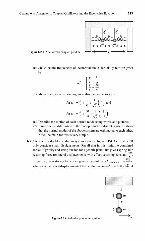
Chapter 6 ■ Asymmetric Coupled Oscillators and the Eigenvalue Equation 213
Figure 6.P.3 A set of two coupled pendula.
(c) Show that the frequencies of the normal modes for this system are givenby
ω2 =
⎧⎪⎨⎪⎩
g
�+ k
mg
�+ 3k
m
(d) Show that the corresponding normalized eigenvectors are:
for ω2 = g
�+ k
m: 1√
2
(11
)and
for ω2 = g
�+ 3k
m: 1√
2
(1
−1
)(e) Describe the motion of each normal mode using words and pictures.(f) Using our usual definition of the inner product for discrete systems, show
that the normal modes of the above system are orthogonal to each other.Note: the math for this is very simple.
6.9 Consider the double-pendulum system shown in figure 6.P.4. As usual, we’llonly consider small displacements. Recall that in this limit, the combinedforces of gravity and string tension for a generic pendulum give a spring-like
restoring force for lateral displacements, with effective spring constantmg
L.
Therefore, the restoring force for a generic pendulum is Fpendulum = −mg
Lx,
where x is the lateral displacement of the pendulum bob relative to the lateral
Figure 6.P.4 A double pendulum system.

214 Waves and Oscillations
position of the support point. (a) Derive the eigenvalue equation (in matrixform) for this system. (b) Now write the characteristic equation, and use itto find the normal mode frequencies. (c) Finally, find the eigenvectors.
6.10 The CO2 molecule. Carbon dioxide is a linear molecule with a carbon atomat the center which is double-bonded to two oxygen atoms, as suggestedin figure 6.P.5. The two springs are identical, and have spring constantk = 3628 N/m. We’ll assume that the carbon atom is a 12C isotope (themost common kind, having six protons and six neutrons), meaning that ithas a mass of exactly 12 u = 1.993 × 10⁻²⁶ kg, and that the oxygen atomsare both 16O, meaning that the mass of each is 2.66 × 10⁻²⁶ kg. Find theeigenvectors and normal mode frequencies for this system. For each normalmode, describe the oscillation in words as well as by giving the eigenvector.(You are encouraged to use a symbolic algebra program such as Mathematicaor Maple for this problem, though it is not necessary.)
6.11 (You should do problem 6.6 before this problem.) Find the normalizedeigenvectors for the system described in problem 6.6.
6.12 (You should do problem 6.7 before this problem.) Find the normalizedeigenvectors for the system described in problem 6.7.
6.13 Consider the system shown in figure 6.P.6. (a) Find the matrix A that appearsin the eigenvalue equation A |e〉 = ω2 |e〉, where |e〉 is an eigenvector. (b) Forthe special case m1 = m2 = 1 kg, m3 = m4 = 2 kg, �α = 1 m, �β = 2 m,
k13 = 2 N/m, k24 = 4 N/m, and g = 4 m/s2, show that∣∣ea
⟩ =⎛⎜⎜⎝
0.653−0.2710.653
−0.271
⎞⎟⎟⎠ is
an eigenvector for this system, without using a symbolic algebra program.
Figure 6.P.5 Model for a CO2 molecule.
Figure 6.P.6 A system of four coupled pendula.

Chapter 6 ■ Asymmetric Coupled Oscillators and the Eigenvalue Equation 215
(c) Determine the angular frequency of oscillation ωa for the mode describedby
∣∣ea
⟩. (d) Make approximate sketches of the positions of the masses for
this mode at t = 0 and at t = π/ωa. (e) Show that∣∣ea
⟩is normalized, without
using a symbolic algebra program.6.14 For the system shown in figure 6.P.6, consider the special case m1 = 1 kg,
m2 = 2 kg, m3 = 3 kg, m4 = 4 kg, �α = 1 m, �β = 2 m, k13 = 3 N/m,
k24 = 6 N/m, and g = 10 m/s2. Use a symbolic algebra program to find thenormalized eigenvectors and corresponding angular frequencies. Make clearwhich eigenvector goes with which angular frequency. For each eigenvector,make a rough sketch of the positions of the masses at t = 0 and at t = π/ω,where ω is the angular frequency for that mode.
6.15 Do not use a symbolic algebra program or calculator for this problem. Theasymmetric coupled pendulum system shown in fig. 6.2.1 has l1 = 1.00 m,l2 = 0.500 m, k = 1.50 N/m, m1 = m2 = 0.500 kg. The masses are releasedfrom rest at t = 0, with initial positions x1 = −0.025 m and x2 = 0.045 m.What are the positions of the two masses as a function of time?
6.16 Let’s define an arbitrary bra 〈g| = (g1 g2
), an arbitrary ket |x〉 =
(x1x2
),
and an arbitrary matrix A =(
a bc d
). Show explicitly that 〈g| A |x〉 is
unambigous, that is, show that(〈g| A
)|x〉 is the same as 〈g|
(A |x〉
).
6.17 Consider the two-pendulum system shown in figure 6.7.2, in which m1= 1 kg, m2 = 2 kg, � = 1 m, k = 1 N/m, and g = 10 m/s2. Verify
that the (unnormalized) eigenvectors for this system are∣∣e1
⟩ =(
11
)
and∣∣e2
⟩ =(−2
1
).

7 String Theory
Midnight. No waves,no wind, the empty boatis flooded with moonlight.
—Dogen (1200–1253)
Each string I touchSends out its love in wavesAnd now the boat is full.
—Marian McKenzie
In some of the most complicated theories of modern physics, elementary particles arerepresented in terms of the normal modes of extremely short (10−35 m) strings. Usually,these theories are hyperdimensional, that is, they use more than the normal number(four) of spacetime dimensions; several string theories have ten dimensions or more.Often, string theorists investigate a slice through this multidimensional space. A slicethrough three-dimensional space has two dimensions, and is called a “membrane.”A slice through a five-dimensional space might have four dimensions, and would becalled a “4-brane.” In general, a slice with p dimensions is called, get this, a “p-brane.”This proves that even the most advanced theoretical physicists have a sense of humor!So far, it has been very difficult to test string theories experimentally.
In this chapter, we will study ordinary macroscopic strings. This will lead usto an understanding of the normal modes of continuous systems, and of how thenormal modes are modified when a system is not truly continuous (e.g., when itconsists of atoms). Surprisingly, our study of strings will also lead us to a fundamentalunderstanding of Fourier analysis, a completely mathematical idea in which anyarbitrary function can be constructed by adding together sine waves. Finally, as inprevious chapters, we will point out the deep connections between these macroscopicoscillating systems and quantum mechanics.
7.1 The beaded string
We begin by considering a massless string of length L stretched between two walls,so that it is under tension T . The string has N beads (each of mass m) spaced at even
216

Chapter 7 ■ String Theory 217
Figure 7.1.1 a: A massless string under tension T with small beads equally spaced along itslength. b: Geometry needed for calculating the force on bead j.
intervals a, as shown in figure 7.1.1a. We assume gravity is unimportant. If the stringis plucked, it vibrates. Each bead feels a force from the string coupling it to the bead onits left, and a second force from the string coupling it to the bead on its right. Therefore,this is a system of N coupled oscillators. As in chapter 6, we expect that such a systemwill display normal modes, and we will use a similar procedure to find out what theyare. For mathematical convenience, we introduce two fictitious beads at the ends ofthe string, as shown.
We wish to find the ways in which this system can move. We follow our multi-stepprocedure.
Step 1: Write FTOT = my for each mass. We will take the approximation of smalldisplacements from equilibrium. In this limit, when the system oscillates the changein the magnitude of the string tension T is negligible. So, from figure 7.1.1b, we seethat the y-component of the force acting on mass j is
FTOT, y = −T sin θL − T sin θR, (7.1.1)
where
sin θL = yj − yj−1√a2 +
(yj − yj−1
)2

218 Waves and Oscillations
For small displacements from equilibrium,(
yj − yj−1
)� a, so we can write
sin θL∼= yj − yj−1
aand similarly sin θR
∼= yj − yj+1
a
Substituting these into equation (7.1.1) gives
FTOT, y = −T
a
(yj − yj−1 + yj − yj+1
)= myj
⇔ − T
ma
(−yj−1 + 2yj − yj+1
)= yj (7.1.2)
Let us define
ωA ≡√
2T
ma. (7.1.3)
This is the angular frequency at which one mass would oscillate if its neighbors wereheld fixed, as you can see by setting yj−1 = yj+1 = 0 in equation (7.1.2). The simplestcomplex equation whose real part is the above would be
−ω2A
2
(−zj−1 + 2zj − zj+1
)= zj, (7.1.4)
where yj = Re zj. Since j can range from 1 to N , this represents a system of Ncoupled DEQs.
Step 2: Use physical and mathematical intuition to guess a solution. Based on ourexperience with the system of two coupled oscillators, we hope that this system maydisplay normal modes, in which each bead moves with the same frequency. The mostgeneral possible such guess would be
zj?= Yj eiωn t . (7.1.5)
Where ωn is the angular frequency of the normal mode, n is the mode index, and Yj isthe amplitude of bead j. (As before, we have chosen the definition of the moment whent = 0 so that the phase of the normal mode ϕ = 0.) We expect for a system of N beadsthat there will be N normal modes, each of which has its own characteristic frequency.
Step 3: Plug the guess into the system of DEQs. Plugging our normal modesguess (7.1.5) into (7.1.4) gives
− ω2A
2
(−Y( j−1)e
iωnt + 2Yjeiωnt − Y( j+1)e
iωnt)
= −ω2nYje
iωnt
⇒ ω2A
2
(−Y( j−1) + 2Yj − Y( j+1)
)= ω2
nYj (7.1.6)
This is a system of N coupled linear equations. In principle, we could solve itusing the methods of section 6.3, that is, we could write it as a matrix eigenvalueequation, rearrange it to a characteristic equation, set the determinant equal to zero tofind the eigenvalues, and plug these back into the characteristic equation to find theeigenvectors.

Chapter 7 ■ String Theory 219
7.2 Standing wave guess: Boundary conditions quantize the allowedfrequencies
Obviously, this procedure would be tedious for a system of more than a few beads.However, we can get to the answer much more quickly by using additional physicalinsight to guess what the eigenvectors are, that is, to guess what the initial positions ofthe beads are for a normal mode. We have all played with ropes, telephone cords, andso on, and have observed “standing waves,” in which the rope oscillates between thepositions shown by the solid lines and the dashed lines in figure 7.2.1. Each part of therope oscillates up and down with the same frequency, so these represent the normalmodes of the system. It is reasonable to expect that the normal modes of the beadedstring would be similar.
In these standing waves, each part of the string oscillates with a different amplitude.From figure 7.2.1c we see that the amplitude of oscillation for a point at position x isgiven by,
amplitude = An sin
(2π
x
λn
),
where λn is the wavelength of the standing wave and An is the amplitude of the standingwave.
Therefore, we will make the following guess for the positions of the beads on thebeaded string:
amplitude = Yj?= An sin
(2π
xj
λn
), (7.2.1)
where xj is the x-position of bead j. This is our “standing wave guess” for the form ofthe eigenvectors; each different value of j in the above equation (corresponding to eachdifferent bead) gives a different line of the column matrix representing the eigenvector.
Figure 7.2.1 a: In the lowest-frequency standing wave (n = 1), the rope oscillates between theshape shown by the solid curve and that shown by the dashed curve. b: Similar curves for then = 2 standing wave. c: The n = 3 standing wave.

220 Waves and Oscillations
Because the string must go to y = 0 at the boundaries, we must fit an integernumber of half-wavelengths between the walls, that is,
nλn
2= L ⇔
λn = 2L
n. (7.2.2)
Since the wavelength cannot take on a continuous range of values, but only thoseallowed by the above equation, we see that the imposition of boundary conditions has“quantized” the allowed values of λ. To save writing (and to follow well-establishedconvention), we define the “wavenumber”
kn ≡ 2π
λn= n
π
L. (7.2.3)
Thus, the wavenumber is 2π divided by the periodicity in space (λ) , just as the angularfrequency ω is 2π divided by the periodicity in time (T ). Using this, equation (7.2.1)can be written
Yj?= An sin
(kn xj
)(7.2.4)
(Again, n is the mode index and j is the mass index.)Figure 7.2.1 shows that the n = 2 mode has one “node,” that is, one spot in the
middle where the rope doesn’t move. The n = 3 mode has two nodes, and so on. Quitegenerally:
Number of nodes + 1 = n.
To see if our standing wave guess for the eigenvectors works, we plug equation (7.2.4)into (7.1.6). (Recall that equation (7.1.6) was obtained by combining FTOT = my withour normal mode guess.) After canceling the common factor of An, this gives
−ω2A
2sin
(knxj−1
)+ ω2
A sin(
knxj
)− ω2
A
2sin
(knxj+1
)?= ω2
n sin(
knxj
).
Now, xj−1 = xj − a, and xj+1 = xj + a, so this becomes
−ω2A
2
[sin
(knxj − kna
)+ sin
(knxj + kna
)]+ ω2
A sin(
knxj
)?= ω2
n sin(
knxj
).
Next we use the standard formula sin (A + B) = sin A cos B + cos A sin B, andrecall that cos (−θ) = cos θ , while sin (−θ) = − sin θ , to obtain
− ω2A
2
[(sin knxj cos kna − cos knxj sin kna
)+
(sin knxj cos kna + cos knxj sin kna
)]+ ω2
A sin(
knxj
)?= ω2
n sin(
knxj
)⇔ −ω2
A sin knxj cos kna + ω2A sin
(knxj
)?= ω2
n sin(
knxj
)⇔ −ω2
A cos kna + ω2A
?= ω2n

Chapter 7 ■ String Theory 221
So, our standing wave guess does work, but only if1
ω2n = ω2
A
(1 − cos kna
). (7.2.5)
Using the trigonometric identity2
1 − cos θ = 2 sin2 θ
2,
Equation (7.2.5) becomes
ω2n = 2ω2
A sin2 kna
2= 2ω2
A sin2(
nπa
2L
). (7.2.6)
Recall that the imposition of the boundary conditions required that λn can only take ondiscrete values, as given by equation (7.2.2), or equivalently that the wavenumber kncan only take on discrete values as given by equation (7.2.3) . Now, we can see thatthe boundary conditions also force ωn to take on discrete values. This is a very generaland very important observation:
Imposition of boundary conditions quantizes the normal mode frequencies.
Exactly the same thing happens in quantum mechanics: imposition of boundaryconditions (i.e., restricting the electron to a finite region of space, such as the regionnear an atomic nucleus) quantizes the allowed frequencies of the wavefunction �,and since E = hω, this is equivalent to quantizing the allowed energies. Thus, we seethat one of the most famous results of quantum mechanics, the idea that an electronin an atom can only take on certain allowed levels of energy, is directly the result ofattributing a wave nature to the electron, and restricting this wave to a small regionin space.
We can see from equation (7.2.6) that the smaller the region is (i.e., the smaller Lis), the greater the interval between allowed frequencies. Similarly in quantummechanics, the more tightly we confine the electron, the larger the interval betweenallowed energies. This effect is important in determining the energy levels of atoms.
1. This is an example of a “dispersion relation,” that is, a relation between ω and k. It’s likely thatall the waves you have studied in previous courses, including standing waves in organ pipes or onviolin strings, had linear dispersion relations, that is, relations in which ω is directly proportional
to k. For example, for electromagnetic waves in vacuum, we have c = λ
T= 2π/k
2π/ω= ω
k⇔
ω = ck. Clearly, the dispersion relation for standing waves on a beaded string, equation (7.2.5)is nonlinear. We’ll discuss dispersion relations in more depth in chapter 9, and explain why theyare called “dispersion relations.”
2. It is not hard to prove this from more fundamental identities:
cos θ = cos
(θ
2+ θ
2
)= cos2 θ
2− sin2 θ
2⇒ 1 − cos θ = 1 − cos2 θ
2︸ ︷︷ ︸sin2
θ
2
+ sin2 θ
2= 2 sin2 θ
2

222 Waves and Oscillations
It also dictates the behavior of electrons that are not tightly attached to any singleatom, such as electrons in metals. Such electrons can roam throughout the metal.Using electron beam lithography, experimentalists can make metal samples that arevery small, down to only about 100 atoms on a side! As the sample is made smaller,they can observe the transition from having a “continuum” of energy levels (becausethe energy interval between levels is too small to observe) to having clearly quantizedlevels. Such “mesoscopic” samples (between the truly microscopic atomic scale andthe macroscopic scale) display many exciting properties, and may form the basis ofnew types of extremely small transistors.
Let us collect all our results. Plugging the standing wave eigenvectors (7.2.4)into our “normal mode guess” equation (7.1.5): zj = Yje
iωnt gives the completedescription of the normal modes:
zj = An sin(knxj
)eiωnt .
The actual displacement of bead j would be given by the real part of this, so that
yj = An sin(
knxj
)︸ ︷︷ ︸
spatialvariation
cos(ωnt
)︸ ︷︷ ︸timevariation
xj = ja λn = 2L
nn = 1, 2, 3, · · · kn = n
π
L
ωn = √2 ωA sin
(nπa
2L
)ωA ≡
√2T
ma
(7.2.7)
System in pure normal mode n.
7.3 The highest possible frequency; connection to waves in acrystalline solid
We know that the number of normal modes should match the number of objects3
in the system (for a system such as this in which the objects can only move in onedimension), that is, that the maximum value of the mode index n should be N . However,from the above, there is no apparent limit on n. Let’s look more carefully. Fromequation (7.2.7), we have that the frequencies of the normal modes are given by
ωn = √2 ωA sin
(nπ
2
a
L
). (7.3.1)
We see right away that the normal mode frequencies can never exceed√
2 ωA, so thatwe already have a hint that the number of normal modes might actually be limited.
3. More generally, the number of normal modes should match the number of degrees of freedom.

Chapter 7 ■ String Theory 223
Figure 7.3.1 A string with three beads.
Figure 7.3.2 ωn versus n for N = 3.
From figure 7.3.1 we see that
L = (N + 1) a. (7.3.2)
Plugging this into equation (7.3.1) gives
ωn = √2 ωA sin
(π
2
n
N + 1
). (7.3.3)
If we plot ωn as a function of n, it clearly reaches a maximum at n = N + 1; this isshown in figure 7.3.2 for the case N = 3. We can already see graphically4 that ω5 = ω3,or more generally that ωN+2 = ωN . This means that at least the time dependence ofthe n = N + 2 “mode” is the same as that of the n = N mode, suggesting that then = N + 2 is not a new mode at all, but rather is really the same as the n = N mode.(Similarly, we can see that the time dependence of the n = N + 3 “mode” is the sameas that of the n = N − 1 mode, etc.)
4. This is also easy to show symbolically: from equation (7.3.3) we have ωN+2 = √2 ωA
sin
(π
2
N + 2
N + 1
)= √
2 ωA sin
(π · 2 (N + 1)
2 (N + 1)− π · N
2 (N + 1)
)= √
2 ωA sin
(π − π · N
2 (N + 1)
).
Now, sin (π − x) = − sin (−x) = sin x. So, ωN+2 = √2 ωA sin
(π
2
N
N + 1
)= ωN .

224 Waves and Oscillations
Does the spatial dependence of the n = N + 2 mode bear out this hunch? Fromequation (7.2.7), we have that for mode n = N + 2
yj = AN+2 sin kN+2xj cos ωN+2 t.
Where AN+2 is the overall amplitude of the mode. The spatial dependence of this is
yj (t =0)=AN+2sinkN+2xj =AN+2sin
(π
N +2
Lxj
)=AN+2sin
(2π
2(N +1)−N
2Lxj
)
=AN+2sin
{2π
[2(N +1)xj
2(N +1)a− N xj
2L
]}=AN+2sin
{2π
[2(N +1)ja
2(N +1)a− N xj
2L
]}
=AN+2sin
{2π j−π
N
Lxj
}=AN+2sin
{−π
N
Lxj
}where the last step works because j is an integer. Finally, since sin (−x) = − sin x and
kN = πN
L, we have
yj (t = 0) = −AN+2 sin(
kN xj
).
This is the same as the spatial dependence of the n = N mode, differing only by aminus sign that can be absorbed into the amplitude.
This is shown graphically in figure 7.3.3; note that the function An sin knxj onlytakes on physical reality at the positions xj of the beads; we can draw the continuousmathematical function An sin knx as shown by the dashed lines, but this does notrepresent the shape of the string. Since the string is massless, it simply forms straightline segments between the beads, as shown by the solid line. The same bead positions
Figure 7.3.3 As shown here for the case N = 3, the mode n = N + 2 gives the same beadlocations (i.e., has the same spatial dependence) as the mode n = N . The mathematicalfunctions A3 sin k3 x (black dashed line) and A5 sin k5 x (gray dashed line) only take onphysical reality at the positions of the beads. Because the string is massless, it follows straightlines (solid lines) between the beads.

Chapter 7 ■ String Theory 225
can be characterized using the black dashed curve (with kN ) or the gray dashed curve(with kN+2).
Thus, since the spatial and time dependence of the n = N + 2 are the same as forn = N , we see that the n = N + 2 mode is not actually a new, independent mode, butis really the same as the n = N mode. We could make similar arguments to show thatthe spatial dependence of the n = N + 3 mode is the same as the n = N − 1 mode,and so on. So, all the modes with n = N + 2 or greater simply reproduce the modeswith n = N or smaller.
But what about the n = N +1 “mode”? We see from figure 7.3.2 that the frequencyfor this “mode” doesn’t match the frequency of any other mode, and yet we know thatthere should be only N modes. The solution to this dilemma comes from consideringthe spatial dependence. For n = N + 1, we have
kN+1 = (N + 1)π
L= (N + 1)
π
(N + 1) a= π
a.
This means that λN+1 = 2π
kN+1= 2a. Therefore, the spatial dependence for this mode
is as shown in the top part of figure 7.3.4. Each bead is at a node, and so the beadsnever move. Therefore, this is not really a “mode,” but rather a very complicated wayof saying that the beads are allowed to remain motionless!
Here’s another way of understanding why there is a highest possible mode, thatis, a shortest possible wavelength. Note that, in the highest actual mode (n = N), thepositions of the masses alternate up–down–up, and so on, as shown in figures 7.3.3and 7.3.4 bottom. Thus, this is the “most wiggliness” that can be represented by thesystem, that is, the shortest wavelength.
Figure 7.3.4 Top: For n = N + 1, each bead is at a node. Bottom: For n = N , there is analternating up-down pattern, so that the string is displaying the most “wiggliness” possible.

226 Waves and Oscillations
These ideas are illustrated further in the applet for this section on the website forthis text.
A crystal is a regular array of atoms. Examples include all metals (usually made ofmany tiny “crystallites” stuck together) and the silicon wafers used to make integratedcircuits. Each atom in a crystal is in stable equilibrium, and therefore (using thearguments of chapter 1) can be modeled as a harmonic oscillator. So, one line of atomsin a crystal can be modeled as a beaded string. Since there is a well-defined highestfrequency of normal mode for a beaded string, there is a well-defined highest frequencyof vibration for a crystal. Because the masses are small, and the restoring forces arerelatively strong, this frequency is fairly high – on the order of about 1013Hz. Thishighest frequency can be observed experimentally – both using spectroscopic methodsand using heat capacity measurements.
7.4 Normal mode analysis for the beaded string
Our analysis in section 6.5 was fully general, and applies perfectly well to the beadedstring. This means that any behavior of the system can be represented as a superpositionof the normal modes. Here’s the way we stated that back in section 6.5:
(6.5.1): |x (t)〉 = Re
[N∑
n=1
Cn eiωnt∣∣en
⟩].
For the beaded string, the beads move in the y-direction, so it makes more sense towrite this as
|y (t)〉 ≡⎛⎜⎝
y1 (t)y2 (t)
...
⎞⎟⎠ = Re
[N∑
n=1
Cneiωnt∣∣en
⟩], (7.4.1)
Normal mode expansion for beaded string
where y1(t) is the position of bead 1, and∣∣en
⟩is the normalized eigenvector for mode n.
We already know the form of the eigenvectors, though they aren’t yet normalized. Insection 7.2, we found that the entries in each line of the eigenvector are
(7.2.4): Yj = An sin(
kn xj
),
so that the eigenvectors are given by
∣∣en
⟩ = An
⎛⎜⎝
sin knx1sin knx2
...
⎞⎟⎠ .

Chapter 7 ■ String Theory 227
To find the normalized eigenvectors, we set⟨en
∣∣ en
⟩ = 1
⇒ A∗n
(sin knx1 sin knx2 · · ·)An
⎛⎜⎝
sin knx1sin knx2
...
⎞⎟⎠ = 1 ⇒ ∣∣An
∣∣2 = 1N∑
j=1sin2 knxj
.
You can show in problem 7.6 that
N∑j=1
sin2 knxj = N + 1
2. (7.4.2)
For convenience, we may as well choose An to be real, so that
An =√
2
N + 1
and
∣∣en
⟩ =√
2
N + 1
⎛⎜⎝
sin knx1sin knx2
...
⎞⎟⎠ (7.4.3)
Normalized eigenvectors for beaded string.
Self-test: Verify that the above is indeed correctly normalized for the case N = 3 andn = 2.
Because the analysis of section 6.5 was fully general, we can find the coefficients Cnin the normal mode expansion (7.4.1) by using the formulas
(6.5.8a): Re Cn = ⟨en | y0
⟩and (6.5.8b): Im Cn = − 1
ωn
⟨en | y0
⟩.
(Here, we have replaced the x’s by y’s to fit the current situation.)
7.5 Longitudinal oscillations
As discussed in section 7.4, the beaded string is a good model for vibrations in asolid. However, the atoms in a solid can vibrate in two distinct ways. So far, we havediscussed transverse vibrations, in which the motion is the y-direction, perpendicularto the direction in which the wavelength is defined (the x-direction). For a solid, thiswould correspond to planes of atoms sliding laterally without changing the distancebetween planes, as shown in the left part of figure 7.5.1. However, the planes of atomscan also vibrate along the x-direction, so that the distance between planes oscillates,as shown in the right part of figure 7.5.1. The one-dimensional model for this type ofoscillation is a chain of beads connected by springs. We measure the x-position of each

228 Waves and Oscillations
Figure 7.5.1 Transverse andlongitudinal oscillations in asolid.
Figure 7.5.2 Quantities defined for longitudinal oscillations.
bead relative to its equilibrium position, however to avoid confusion with the variablex, we describe this displacement using the symbol δ, as shown in figure 7.5.2.
Your turn: Explain why the total force on bead j is FTOT = −k(δj − δj−1
)− k
(δj − δj+1
).
Since FTOT = mδj, this gives
− k
m
(−δj−1 + 2δj − δj+1
)= δj. (7.5.1)
This equation is isomorphic with equation (7.1.2), the differential equation describingtransverse oscillations on the beaded string:
− T
ma
(−yj−1 + 2yj − yj+1
)= yj.
Table 7.5.1. Isomorphism between transverse and longitudinal waves
Quantity Transverse Longitudinal
Displacement yj δj
Angular frequency of vibrationwith neighbors fixed
ωA =√
2Tam ωA =
√2km

Chapter 7 ■ String Theory 229
Thus, the solutions are exactly the same as for transverse vibrations, with thesubstitutions indicated in table 7.5.1 above, giving
δj = An sin(
knxj
)︸ ︷︷ ︸
spatialvariation
cos(ωnt
)︸ ︷︷ ︸timevariation
xj = ja λn = 2L
nn = 1, 2, 3, · · · kn = n
π
L
ωn = √2 ωA sin
(nπa
2L
)ωA ≡
√2k
m
(7.5.2)
System in pure normal mode n
Figure 7.5.3 shows the vibrations of the mode n = 1. At t = 0, all the beads aredisplaced to the right, resulting in a bunching near the right side. A half period later,the beads are all displaced to the left, resulting in bunching near the left side.
Let’s apply this model to a thin solid rod of cross-sectional area A, which is wedgedbetween two massive walls, with one end of the rod pushing against each wall. Wetreat each plane of atoms perpendicular to the axis of the rod as a bead, with massm = ρAa, where a is the spacing between atomic planes. From equation (2.3.2), the
spring constant of a solid with cross-sectional area A and length a is k = EA
a, where
Figure 7.5.3 Displacements at t = 0 and half a period later for the mode n = 1 for longitudinaloscillations.

230 Waves and Oscillations
E is the Young’s modulus. Thus, ωA =√
2k
m=
√2EA
ρAa2= 1
a
√2E
ρ. If we consider, for
example, the low n modes of a rod with at least several mm of length, we have na � L,so that
ωn = √2 ωA sin
(nπa
2L
) ∼=√
2 ωAnπa
2L,
where we have used the approximation (1.6.4): sin θ ∼= θ , valid for small θ . Therefore,
ωn∼=
√2
1
a
√2E
ρnπa
2L= n
√E
ρ
π
L. (7.5.3)
7.6 The continuous string
It is easy to extend the results of section 7.4 to a continuous string with finite mass.We simply imagine shrinking the distance a between the beads (by adding more beadsonto the string), while also making the beads less massive, so as to keep the mass perunit length constant. Then, in the limit a → 0 (and N → ∞), we have a continuous,massive string.
We can readily find the frequencies of the normal modes in this limit. Fromequation (7.2.7), we have for the beaded string
ωn = 2
√T
masin
(nπa
2L
)= 2
√T
masin
(π
2
n
N + 1
).
In the limit N → ∞, the argument of the sin becomes infinitesimal, so we can use
sin x −−→x→0
x.
Therefore, as we allow N → ∞, we obtain
ωn = 2
√T
ma
(nπa
2L
)= √
T
√a
mnπ
L. (7.6.1)
We define the mass per unit length:
μ ≡ m
a,
so that equation (7.6.1) becomes
ωn = nπ
L
√T
μ= nω1, (7.6.2)
Normal mode frequencies for continuous string
where ω1 = π
L
√T
μ. Note that, unlike for the beaded string, these frequencies are all
multiples of the fundamental frequency ω1, and that they increase linearly with themode index n. One way to understand this is by considering the graph of ωn for thebeaded string, as shown in figure 7.6.1. The peak of this graph is at n = N + 1, so
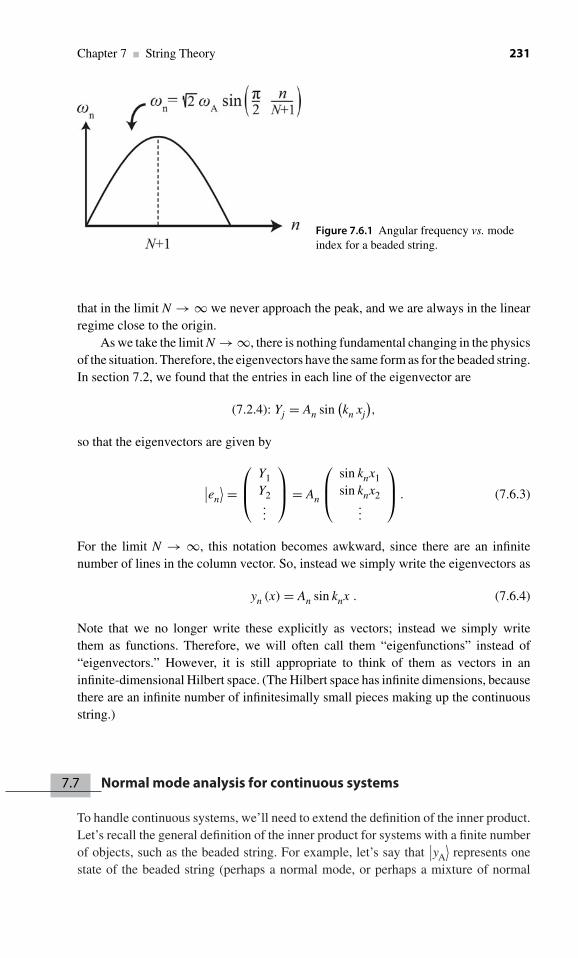
Chapter 7 ■ String Theory 231
Figure 7.6.1 Angular frequency vs. modeindex for a beaded string.
that in the limit N → ∞ we never approach the peak, and we are always in the linearregime close to the origin.
As we take the limit N → ∞, there is nothing fundamental changing in the physicsof the situation. Therefore, the eigenvectors have the same form as for the beaded string.In section 7.2, we found that the entries in each line of the eigenvector are
(7.2.4): Yj = An sin(kn xj
),
so that the eigenvectors are given by
∣∣en
⟩ =⎛⎜⎝
Y1Y2...
⎞⎟⎠ = An
⎛⎜⎝
sin knx1sin knx2
...
⎞⎟⎠ . (7.6.3)
For the limit N → ∞, this notation becomes awkward, since there are an infinitenumber of lines in the column vector. So, instead we simply write the eigenvectors as
yn (x) = An sin knx . (7.6.4)
Note that we no longer write these explicitly as vectors; instead we simply writethem as functions. Therefore, we will often call them “eigenfunctions” instead of“eigenvectors.” However, it is still appropriate to think of them as vectors in aninfinite-dimensional Hilbert space. (The Hilbert space has infinite dimensions, becausethere are an infinite number of infinitesimally small pieces making up the continuousstring.)
7.7 Normal mode analysis for continuous systems
To handle continuous systems, we’ll need to extend the definition of the inner product.Let’s recall the general definition of the inner product for systems with a finite numberof objects, such as the beaded string. For example, let’s say that
∣∣yA
⟩represents one
state of the beaded string (perhaps a normal mode, or perhaps a mixture of normal

232 Waves and Oscillations
modes), and that∣∣yB
⟩represents some different state. We can write
∣∣yA
⟩ =⎛⎜⎝
yA1yA2...
⎞⎟⎠ and
∣∣yB
⟩ =⎛⎜⎝
yB1yB2...
⎞⎟⎠ ,
where, for the state∣∣yA
⟩, yA1 is the position of bead 1, yA2 is the position of bead 2,
and so on.The inner product is defined as
⟨yA | yB
⟩ ≡ (y∗
A1 y∗A2 · · ·)
⎛⎜⎝
yB1yB2...
⎞⎟⎠ =
N∑j=1
y∗AjyBj . (7.7.1)
For a continuous system, there would be an infinite number of objects, so this wouldbecome an infinite sum, which we can write using an integral. Therefore, we definethe inner product of two continuous functions yA (x) and yB (x) to be
⟨yA (x) | yB (x)
⟩ ≡L∫0
y∗A (x) yB (x) dx, (7.7.2)
where the range x = 0 to x = L is the size of the continuous system. For a systemwith a differently defined size, the limits of integration would be changed, so that theintegral is still over the entire system.
Although equation (7.7.2) is the well-established convention for the definitionof the inner product, it is not quite equivalent to the definition (7.7.1) for discretesystems, since each term in the sum which the integral represents is multiplied by theextra factor dx. It should be clear that, even with this extra factor, the eigenfunctionsare still orthogonal (i.e., the inner product of two different eigenfunctions is still zero),since zero times dx is still zero.
5. From equation (7.6.3), we have yn (x) = An sin knx and ym (x) = Am sin kmx. According to
equation (7.7.2), their inner product is⟨yn (x)
∣∣ ym (x)⟩ =
L∫0
A∗n sin knx Am sin kmx dx = A∗
nAm ×[sin
(kn − km
)x
2(kn − km
) − sin(kn + km
)x
2(kn + km
)]L
0
. Recall that kn = nπ
L, so that kn − km = (n − m)
π
L
and kn + km = (n + m)π
L. Therefore,
⟨yn (x)
∣∣ ym (x)⟩ = A∗
nAm
[sin [(n − m) π]
2(kn − km
) −
sin [(n + m) π]
2(kn + km
) − 0 + 0
]. Since n and m are integers, this equals zero, Q.E.D.

Chapter 7 ■ String Theory 233
Self-test (answer below5): Verify that the eigenfunctions yn (x) and ym (x) for thecontinuous string are indeed orthogonal if n �= m. You may need this integral, givenin the form you would find it in an integral table:∫
sin px sin qx dx = sin(p − q
)x
2(p − q
) − sin(p + q
)x
2(p + q
) p �= ±q
(Although this is the common way to write this, it is somewhat ambiguous; it shouldbe read ∫
sin px sin qx dx = sin[(
p − q)
x]
2(p − q
) − sin[(
p + q)
x]
2(p + q
) p �= ±q
Your turn: Show that the normalized eigenfunctions for the continuous string aregiven by
yn (x) =√
2L
sin knx (7.7.3)
Ignore the following paragraph if it confuses you, but you might find itinteresting. Compare equation (7.7.3) with the normalized eigenvectors for the beadedstring:
(7.4.3):∣∣en
⟩ =√
2
N + 1
⎛⎜⎝
sin knx1sin knx2
...
⎞⎟⎠
Normalized eigenvectors for beaded string
By recalling that L = (N + 1) a, we see that the result (7.7.3) for the continuous stringis the same as that for the beaded string, except that the continuous string result isdivided by
√a; for the continuous string, the “spacing” between “beads” is a = dx, so
that the normalized eigenfunctions have been divided by√
dx . When we take the innerproduct of two such functions, we effectively divide by
√dx twice; this compensates
for the “extra” factor of dx in the definition of the inner product that was discussed atthe top of the previous page.
You should recall that the normalized eigenvectors for discrete systems weredimensionless. From equation (7.7.3), we can see that the normalized eigenfunctionsfor the continuous string have units of meters −1/2. This might seem strange, but itis indeed correct, and necessary to make the normal mode analysis formulas workout correctly. It might make you feel better to know that the wave function for one-dimensional quantum mechanics (analogous to our one-dimensional continuous string)also has units of meters −1/2.
234 Waves and Oscillations
As for the beaded string (and the coupled pendula), any state of the system can bewritten as a superposition of the normal modes, that is,
y (x, t) = Re
[ ∞∑n=1
Cneiωntyn (x)]
. (7.7.4)
Normal mode expansion for continuous string
(If the system is truly continuous, then there are an infinite number of normal modes.)Because the analysis of section 6.5 was fully general, we can find the coefficients Cnin the normal mode expansion (7.7.4) by using the formulas
(6.5.8a): Re Cn = 〈yn(x)|y0(x)〉 and
(6.5.8b): Im Cn = − 1
ωn〈yn(x)|y0(x)〉 .
(Here, we have replaced the x’s by y’s, and vectors by functions to fit the currentsituation.) Again, for the important special case y0 (x) = 0, the process of normalmode analysis is exactly analogous to the process of taking projections of ordinaryvectors onto the x- and y-axes (although now there are an infinite number of axes ontowhich we must take projections!).
7.8 k-Space
As for the other coupled oscillator systems that we’ve studied, we can fully specifythe behavior of the continuous string either by specifying y (x, t) or by specifyingall the amplitudes Cn in the normal mode expansion. Let’s consider the importantspecial case y0 (x) = 0, for which Im Cn = 0. Then, we can write the normal modeexpansion (7.7.4) as
y(x, t) =N∑
n=1
Cn cos ωnt yn (x) ,
where Cn = Re Cn = ⟨yn (x) | y0 (x)
⟩Normal mode expansion for y0 (x) = 0.
At t = 0, this reduces to
y(x, t = 0) =√
2
L
N∑n=1
Cn sin knx. (7.8.1)
Each Cn is associated with a kn. We could thus make a plot of Cn versus k, as shownin figure 7.8.1 for a particular y (x, t = 0) which involves mixing several normalmodes. The initial shape of the string can be specified either by plotting y versusx, or by plotting Cn versus k. The latter view is called “k-space.” We can make a

Chapter 7 ■ String Theory 235
Figure 7.8.1 k-space for the continuous string.
Figure 7.8.2 Three-dimensional view of normal mode analysis at t = 0. (Note that the pictureis somewhat schematic. For example, the actual perspective from viewpoint B would not allowone to tell whether each Cn was positive or negative.)
three-dimensional plot, as shown in figure 7.8.2, which symbolizes the process ofnormal mode analysis at t = 0. Looking from viewpoint A, we can imagine adding upthe sinusoids to produce y (x, t = 0); this is the real space view. However, we could justas well look from viewpoint B, which gives the k-space view. This idea of looking atthings in k-space turns out to be tremendously important in crystallography, solid-statephysics, and many other areas.

236 Waves and Oscillations
Concept and skill inventory for chapter 7
After reading this chapter, you should fully understand the following
terms:
Standing wave (7.2)Wavenumber (7.2)Dispersion relation (7.2)Longitudinal waves (7.5)k-space (7.8)Real space (7.8)
You should understand the following connections:
Boundary conditions & allowed frequencies (7.2)Mode index & number of nodes (7.2)Bead spacing & maximum wiggliness (7.3)Transverse & longitudinal oscillations (7.5)Normal modes for beaded & continuous strings (7.6)Hilbert space vectors & continuous functions (7.6)Representations of a function in real space & in k-space (7.8)
You should be familiar with the following additional concepts:
Highest frequency/smallest wavelength standing wave for a beaded string (7.3)Functions only taking on physical reality at certain positions (7.3)
You should be able to:
Find the frequency for a given normal mode of a beaded string (7.2)Explain why there is a minimum wavelength for standing waves on a beaded
string (7.3)Analyze a given pattern of initial velocities and positions for a beaded string into a
superposition of normal modes (7.4)Find the frequency for a given normal mode of a continuous string (7.6)Analyze a given pattern of initial velocities and positions for a continuous string into
a superposition of normal modes (7.7)Take inner products of continuous functions (7.7)
In addition to all of the above, you should be able to combine the concepts
you’ve learned to address new situations.
Problems
Note: Additional problems are available on the website for this text.

Chapter 7 ■ String Theory 237
Instructor: Ratings of problem difficulty, full solutions, and important additionalsupport materials are available on the website.
7.1 State what is wrong with the following: “When a beaded string is in purenormal mode 2, the displacement of bead 1 is given by A sin k1x2 cos ω1t,where A is the amplitude of motion of the bead.” (There might be more thanone thing wrong.)
7.2 Orthogonality of normal modes for the beaded string
(a) Find the normalized eigenvectors for the beaded string with N = 3.Let’s call them
∣∣e1
⟩,∣∣e2
⟩, and
∣∣e3
⟩. (The subscripts here refer to the
mode index n, not to the mass index j.)(b) Show that
⟨en | en
⟩ = 1 for all possible values of n, thus verifyingthat you have correctly normalized the eigenvectors.
(c) Show that⟨en | em
⟩ = 0 for all possible combinations of n and mwhere n �= m, thus verifying that the eigenvectors are mutuallyorthogonal.
7.3 Beaded string appletGo to the website for this text, and under chapter 7 open the “Beaded StringApplet.”
Write out answers to all questions in boldface.
(a) This applet demonstrates some properties of standing waves on abeaded string. You may select the number of beads (masses) and thedesired normal mode to display with the two sliders at the bottom ofthe applet. Additionally, you may at any time choose to slow downthe animation with the “Slow” check box.
(b) First, look at a string with 4 beads on it. Set that up using the“masses” slider. Now look at the normal modes for this configurationby varying the “mode” slider. How many normal modes are there?Try a few other configurations consisting of different numbers ofbeads. In general, for this one dimensional case (beads can onlymove up and down), how does the number of normal modesrelate to the number of beads?
(c) The main goal of this applet is to visually demonstrate the fact thatthere is a maximum meaningful normal mode index n for waves ona beaded string. As we have just seen, the maximum index relatesto the number of beads on the string. What happens if you try togenerate normal modes with indices higher than the maximumpossible mode for a situation? Try it. What do the blue andred waves represent? Explain why these two waveforms do notrepresent the actual string. What would the actual string looklike? Take a moment to try the animation with a number of differentnormal mode frequencies and numbers of beads. Think about whatyou have seen.
(d) Explain what the graph in the lower left represents. Why is theright part shown as a dashed line?

238 Waves and Oscillations
(e) If there is a maximum normal mode index for a beaded string,what does this imply about the possible frequencies of waves thatcan exist on the string? Explain. What does this imply aboutwaves in a crystal lattice (which can be thought of as a threedimensional array of beads on springs)?
(f) Given the normal modes for a beaded string, could one constructa Hilbert space to represent this system? What would it looklike? How many dimensions would it have?
7.4 Driven beaded string. A string with N beads, each of mass m and spacinga, is under tension T . At the left, the string is attached to a fixed wall, asusual. However, on the right, it is attached to a wall which oscillates upand down with amplitude h and angular frequency ωd. This means that the“fictitious bead” on the left has y0 ≡ 0 as usual, but the fictitious bead onthe right has yN+1 ≡ h cos ωdt. The differential equations of motion for thissystem are the same as for the undriven case (because the way the beadsinteract with each other is unchanged); only the boundary conditions aredifferent.
(a) Explain why it’s reasonable to guess that a solution for this problem
would be yj?= Yj cos
(ωdt − δ
).
(b) Given the form of the above guess, explain why we expect that Yjneed not equal yj0.
(c) Since the differential equations of motion are the same as for theundriven case, it’s reasonable to guess that the amplitudes Yj varywith position in the same way, that is, it’s reasonable to guess
Yj?= A sin α xj, where the values of A and α are to be determined.
Use yN+1 ≡ h cos ωdt to find δ and A in terms of α, h, a, and N .
(d) Plug our guesses yj?= Yj cos
(ωdt − δ
)and Yj
?= A sin α xj into theequation (7.1.2) (which was derived simply by applying F = mx tomass j):
− T
ma
(−yj−1 + 2yj − yj+1
)= yj
Verify that the guesses work, and show that cos (α a) = 1 −ω2
d(2
T
ma
) .
(e) Explain why the above implies that if ωd > 2
√T
mathen α is
complex. Hint: Set α = αr + iαi, use cos (α a) = Re[eiα a
], and
show that for ωd > 2
√T
ma, αi must be nonzero.
(f ) Explain why a complex value of α means that the wave dampsexponentially in space. Hint: recall that sin x = Im
[eix
].
(g) What does that phrase “damps exponentially in space” mean?

Chapter 7 ■ String Theory 239
(h) Why is it reasonable that the frequency 2
√T
mashould be the highest
frequency which does not give exponential damping in space?
7.5 Normal mode analysis for the beaded string. (You are encouraged to useMathematica, Maple, or other symbolic algebra program for this problem,though it is not necessary.) A beaded string has three beads, each of mass1.00 kg, spaced at 1.00 m intervals. The string has tension 100 N. The initialpositions and velocities of the beads are:
y1 = −2.55033 cm y1 = −35.8043 cm/s
y2 = 3.51028 cm y2 = 1.38233 cm/s
y3 = −0.885746 cm y3 = 15.6333 cm/s
(a) Write explicit equations for y1 (t) , y2 (t) , and y3 (t) that are validfor all times. Your equations should be in terms of cosines, ratherthan Re
[eiωt
]. Note: Remember that the arctan returns a result
that is only defined up to an additive factor ofπ .Therefore, thinkcarefully about the result your calculator or program returnsto you – is it in the correct quadrant of the complex plane? Ifnot, you need to add π to it.
(b) Plug t = 0 into your expressions from part (a), and verify that theygive the correct values for the initial positions.
7.6 Show thatN∑
j=1sin2 knxj = N + 1
2, where kn = nπ
L, xj = ja, L = (N + 1) a,
and n and N are integers. (We used this result in section 7.4.) You shouldprobably use a symbolic algebra program for this; please see the additionalinstructions on the web page for this book.
7.7 Fret spacing on guitars. (Read problem 5.1 before doing this problem; youneed not actually do that problem first, though.) A standard guitar has sixstrings. Each is held under tension, stretched between the bridge (near themiddle of the main body of the guitar) and the nut (near the end of the neck),as shown in figure 7.P.1. A series of frets is positioned just below the strings.When the guitarist uses a finger just behind one of the frets to push one ofthe strings against the fretboard, the effective length L of the string is thedistance from the bridge to the fret, as shown. The frets are spaced so that theguitarist can create notes in half-step intervals. For example, if the higheststring is plucked without using any fret, then the full length of the string(from the bridge to the nut) vibrates, producing a note of E above middle C.(The main pitch produced is from the fundamental, i.e., the n = 1 mode.)If the guitarist pushes down behind the first fret (the one closest to the nut),and then plucks the string, it instead produces an F#. If the guitarist pushesdown behind the second fret, the string produces an F#. If the length frombridge to nut is L0, what is the equation that determines the position forfret number j, where j = 1 for the fret closest to the nut, and positions are

240 Waves and Oscillations
Figure 7.P.1 Top: The frets on a guitar allow the guitarist to vary the effective length of eachstring in a controlled way. Bottom: side view of a finger pressing a string down behind a fret.(Top image © Milinz | Dreamstime.com)
measured relative to the bridge? (Recall from problem 5.1 that the ratio offrequencies for notes that are a half-step apart is 1.05946.)
7.8 Harmonics on guitars. Rather than using the frets (see problem 7.7),guitarists sometimes use an alternate technique. Instead of using a fingerto press the string against the fretboard, the finger is placed lightly on thestring, at a carefully selected point. The string is plucked, and then, as quicklyas possible, the lightly pressing finger is released. The string emits a note thatis bell-like in tone. If the lightly pressed finger is placed at a point halfwayalong the length of the string, the frequency of the note sounded is twicethat of the fundamental frequency of the string. Explain what is happening.(Various such “harmonics” can be produced by different placements of thelightly pressed finger. These can be used to produce notes much higherthan the guitar could ordinarily make. For an example, go to the websitefor this text, and under this chapter find the listing for this problem. Thistechnique is also very important for rock guitarists; you can see lots ofexamples by doing an internet video search using the words rock guitarharmonics.)
7.9 You can make a crude musical instrument by stretching a rubber bandand plucking it. Try it. This will work best with a relatively thick band,held close to your ear. For the most reproducible results, hook your fingersthrough the band, rather than pinching it between your fingers. Important:you should notice that the band stretches fairly easily to a certain length, andthen becomes much stiffer. We will concentrate on the range of fairly easy

Chapter 7 ■ String Theory 241
stretching. Start with the band stretched most of the way, and slowly let itrelax as you pluck it again and again, holding it very close to your ear so youcan hear clearly. Let it relax all the way to the point where it is slack. Then,stretch it out most of the way, and listen again as you let it relax. Using theideas you’ve learned in this book, make a simple quantitative model for howthe pitch should depend on length, and compare your model qualitativelywith your observations. (You will probably find that the behavior is morecomplicated if you start with the band slack and stretch it out than it isif, as directed, you start with it stretched and allow it to relax. This showsthat the model you have developed doesn’t capture all the physics of thissituation.)
7.10 Areasonably accurate model for the dispersion relation of an actual stretchedpiano string is
ω = ak + bk3,
where a and b are constants. Find an expression for all of the possibleoscillatory frequencies of a piano string of length L.
7.11 A string of mass M and length L is attached to walls at either end, and isunder tension T . The string is held at rest in the following shape: y = B forL
2< x <
3L
4, and y = 0 for the rest of the string. The string is released
at t = 0. (a) Find y(x, t). You may express your answer as an infiniteseries, so long as you have defined all the symbols in your series. (b) Usingwords, diagrams, and equations, describe what you did in part a by makinganalogies with a system of conventional two-dimensional vectors in ordinaryx − y space.
7.12 (You may wish to complete problem 7.11 first.) A string of mass M andlength L is attached to walls at either end, and is under tension T . At t = 0,
the string has the following shape: y = B forL
2< x <
3L
4, and y = 0 for the
rest of the string. At t = 0 the velocity distribution is y = E forL
4< x <
L
2,
and y = 0 for the rest of the string. E has units of m/s. Given these initialconditions, find y(x, t). (Note that this velocity pattern is not the same as theinitial position pattern – one is nonzero on the right side of the string, andthe other is nonzero on the left side of the string.) You may express youranswer as an infinite series, so long as you have defined all the symbols inyour series.
7.13 A continuous string with mass per unit length μ is stretched with tension Tbetween two walls, one at x = 0 and the other at x = L. At t = 0, its shape
is given by y (x, t = 0) = L
100
x2
L2, and it is at rest. What is the complex
coefficient for the n = 2 mode in the normal mode expansion for theseinitial conditions? You may need the following integral (given in the formyou would find it in an integral table):∫
x2 sin ax dx = 2x
a2sin ax +
(2
a3− x2
a
)cos ax.

242 Waves and Oscillations
7.14 A string of mass M and length L is attached to walls at either end, and isunder tension T . Prior to t = 0, the string is held fixed with the followingshape:
y0(x) =
⎧⎪⎪⎨⎪⎪⎩
4
L2Gx2 0 ≤ x ≤ L
24
L2G(x − L)2 L
2≤ x ≤ L
⎫⎪⎪⎬⎪⎪⎭ , where G is a constant.
(a) Sketch this shape.(b) At t = 0, the string is released. For the normal mode expansion,
briefly explain why it is unnecessary to calculate the imaginaryparts of the expansion coefficients.
(c) Calculate the coefficients in the normal mode expansion. It mightbe helpful to note the solutions to the following integrals:∫
x2sinAx dx= (2−A2x2)cos(Ax)
A3+ 2xsin(Ax)
A2∫(x−B)2sin(Ax)dx= (2−A2(B−x)2)cos(Ax)+2A(x−B)sin(Ax)
A3.
(d) You should have found that coefficients for the even n terms in theexpansion are all zero. Explain why, based on symmetry.
(e) Write an expression for y(x, t). You may express your answer as aninfinite series, so long as you have defined all the symbols in yourseries.
7.15 At t = 0, the shape of a string under tension T which has mass/length μ isa complicated shape, as shown in figure 7.P.2, and the string is motionlessat this instant. (The vertical scale is greatly exaggerated; displacement fromequilibrium is actually small, so that our usual approximations work well.)The distance between the walls is L. Assume damping is negligible. It is
Figure 7.P.2 Top: Initial shape of string. Bottom:inverse of the original shape.

Chapter 7 ■ String Theory 243
observed that at t = τ , the string returns to exactly the same shape. Theshape also recurs at t = 2τ , 3τ , and so on.
(a) Using ideas of normal mode analysis, explain this surprising result,and also find the value of τ in terms of the other parameters above.
(b) Explain why the inverse of the original shape, that is, the one shownin the lower part of the figure, is never observed.
7.16 The particle in a box. In section 1.11, we discussed the quantum mechanicalwavefunction � (x, t). As you will learn in a later course on quantummechanics, it is governed by Schrödinger’s equation:
− h2
2m
∂2�
∂ x2+ U (x) � = ih
∂�
∂ t,
where h is Plank’s constant, m is the mass of the particle (usually an electron),U(x) is the potential energy the particle would have at position x, and � =� (x, t) is the “wave function” which describes the particle. Note that thisis a linear differential equation, so that we can superpose solutions for it
just as we did for the string stretched between two walls. The notation∂�
∂tmeans “partial derivative of � with respect to x.” This simply means “takethe derivative of � with respect to t, treating x as a constant.” Similarly,
the notation∂2�
∂x2means “second partial derivative of � with respect to x”,
which means “take the second derivative of � with respect to x, treating t asa constant.” You should not get too worried about this notation; it is neededbecause y is a function of both x and t, but there is really nothing mysteriousabout it.
You can see right away, from the presence of the “i” in the above equationthat � is intrinsically complex. Therefore, in what follows there is no needto think about taking real parts of anything.
Consider a particle in the potential U ={
0 0 < x < L∞ x < 0 or x > L
. If the
particle has a finite total energy then it cannot exist outside the region x = 0to x = L, since outside this region its potential energy would exceed its totalenergy by an infinite amount. Therefore, the boundary conditions are that� must go to zero at x = 0 and at x = L. This is very analogous to whathappens to y for a continuous string stretched between two walls.
(a) We can guess that the normal modes of this “particle in a box”system are given by
�n ={
Cn ψn (x) e−iωnt inside the well0 outside the well
,
where the functions ψn (x) = A sin knx are the normalized eigen-functions, and A is a constant that you’ll determine in part (c) ofthis problem. Verify that this guess is correct by plugging it intothe Schrodinger equation and showing that it works. As part ofdoing this checking, you should find the dispersion relation that

244 Waves and Oscillations
is required to make the guess work. (Note that this guess hasthe factor e−iωnt , rather than the factor eiωnt that you might haveexpected from our discussion of standing waves on a rope. For therope waves, since we take the real part anyway, it wouldn’t havemade a difference to include the minus sign in the exponential,although we followed well-established convention by not includingit. As you can see from this exercise, the minus sign really is neededin the quantum mechanical version.)
(b) What is the condition on kn in order for the boundary conditions tobe satisfied?
(c) Find the value of A that correctly normalizes the eigenfunctions forthis situation. You may do this mathematically, or by referring toresults we have previously obtained.
(d) Make an argument for why the eigenfunction for the lowest-frequency normal mode is orthogonal to the eigenfunction for thesecond lowest-frequency normal mode. Note that a response suchas, “All eigenfunctions are orthogonal.” is not acceptable; you mustdemonstrate that the eigenfunctions are orthogonal by mathematicalor logical argument.
(e) Now consider this particular initial condition: At t = 0, � =⎧⎨⎩B
L
4< x <
L
20 elsewhere
. Explain why this means that all the coefficients
Cn that appear in the normal mode expansion of � must be real.Hint: This is a consequence of the fact that � is real everywhereat t = 0. Also, recall that there is no Re[…] in the normal modeexpansion for this situation, as indicated by the boldface text in theintroduction to this problem.
(f) Given the initial conditions of part (e), find� (x, t).You may expressyour answer in terms of an infinite series, so long as all quantities inthe series are explicitly defined, including evaluation of all integrals.Hint: As you showed in part e, all the coefficients Cn are real.Recall that, for a string stretched between two walls we get thatall real coefficents if all the initial velocities are zero. Therefore,having a quantum mechanical wavefunction � that is initially realeverywhere is fully analogous to a stretched string with zero initialvelocity everywhere.
(g) Now, consider a different initial condition, which is formed bysuperposing equal amplitudes of the second-lowest-frequency nor-mal mode and the third-lowest-frequency normal mode. The result-ing superposition shows a “sloshing” back and forth of � (x, t).What is the period of this sloshing, in terms of h, m, and L ? Explain.
7.17 k-space picture for plucked guitar string. The tonal quality of a notesounded by a guitar string depends on where along its length the string isplucked. (For this problem, assume the string is played at full length, withoutusing any frets.) The graphs in figure 7.P.3 show the k-space picture for two

Chapter 7 ■ String Theory 245
Figure 7.P.3 Two possible k-space graphs.
different plucking positions, with amplitude on the vertical axis and k onthe horizontal axis. The scales are the same for both graphs. For one of thegraphs, the string was plucked at the halfway point, that is, a finger halfwayalong the length of the string pulled it slightly away from equilibrium andthen released it. For the other picture, the string was plucked one quarterof the way along its length. Which graph is which? Explain your reasoningthoroughly, including an explanation for why some of the peaks are missingfrom one of the graphs.
8 Fourier Analysis
You need to move past Fourier transfers, and start thinking quantum mechanics.—Maggie Madsen, signal analyst character, the Transformers movie (2007).
8.1 Introduction
Although the above quote is a bit mangled (presumably the writer meant “Fouriertransforms”), it accurately conveys that the first thing any scientist does with acomplicated data set is to subject it to Fourier analysis, that is, the scientist findshow the data can be expressed as a sum of sinusoids. As with normal mode analysis,this gives a powerful and drastically different view of the data, one that is often veryrevealing. Fourier analysis is absolutely omnipresent in modern technology. The jpgimage compression algorithm is based on Fourier analysis. The performance of fiberoptic cables is evaluated using Fourier analysis. Diffraction methods used to determinethe structure of proteins are based on Fourier analysis.1
As an example of how illuminating this method can be, consider the function y(x)shown in the left part of figure 8.1.1. It appears quite irregular, and would be difficult todescribe in any simple way. However, this is just the sum of the three sinusoids shownin the middle part of the figure. The right part shows a graph of the amplitude of thesinusoids (in other words the factor A in A cos (kx + ϕ)) as a function of wavenumber
k = 2π
λ), and a graph of the phase ϕ of the sinusoids. This is just as complete a
description as the graph of y(x), yet it is much more revealing. In this chapter, we will
1. Joseph Fourier (1768–1830) lived a varied and tempestuous life. He was a strong supporter ofthe French revolution, but later became aghast at the excesses of the Terror, and tried to withdrawfrom the committee. This almost led to his beheading. He was sent to Egypt by Napoleon, alongwith 164 other scholars, to “civilize” the country. Fourier spent three years there catalogingantiquities and other discoveries. This exposure to warm climates may be responsible for hishabit of keeping his rooms uncomfortably warm, while wearing a heavy coat. He made importantcontributions to the study of heat propagation, and it was in this connection that he developedthe idea of summing sinusoids to represent other functions. However, this notion met with agreat deal of resistance from the leading French mathematicians of the time, including Laplace,Legendre, and Poisson.
246
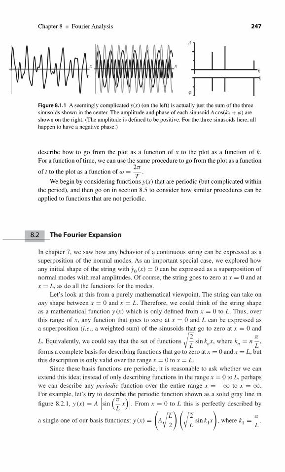
Chapter 8 ■ Fourier Analysis 247
Figure 8.1.1 A seemingly complicated y(x) (on the left) is actually just the sum of the threesinusoids shown in the center. The amplitude and phase of each sinusoid A cos(kx + ϕ) areshown on the right. (The amplitude is defined to be positive. For the three sinusoids here, allhappen to have a negative phase.)
describe how to go from the plot as a function of x to the plot as a function of k.For a function of time, we can use the same procedure to go from the plot as a function
of t to the plot as a function of ω = 2π
T.
We begin by considering functions y(x) that are periodic (but complicated withinthe period), and then go on in section 8.5 to consider how similar procedures can beapplied to functions that are not periodic.
8.2 The Fourier Expansion
In chapter 7, we saw how any behavior of a continuous string can be expressed as asuperposition of the normal modes. As an important special case, we explored howany initial shape of the string with y0 (x) = 0 can be expressed as a superposition ofnormal modes with real amplitudes. Of course, the string goes to zero at x = 0 and atx = L, as do all the functions for the modes.
Let’s look at this from a purely mathematical viewpoint. The string can take onany shape between x = 0 and x = L. Therefore, we could think of the string shapeas a mathematical function y (x) which is only defined from x = 0 to L. Thus, overthis range of x, any function that goes to zero at x = 0 and L can be expressed asa superposition (i.e., a weighted sum) of the sinusoids that go to zero at x = 0 and
L. Equivalently, we could say that the set of functions
√2
Lsin knx, where kn = n
π
L,
forms a complete basis for describing functions that go to zero at x = 0 and x = L, butthis description is only valid over the range x = 0 to x = L.
Since these basis functions are periodic, it is reasonable to ask whether we canextend this idea; instead of only describing functions in the range x = 0 to L, perhapswe can describe any periodic function over the entire range x = −∞ to x = ∞.For example, let’s try to describe the periodic function shown as a solid gray line in
figure 8.2.1, y (x) = A∣∣∣sin
(π
Lx)∣∣∣. From x = 0 to L this is perfectly described by
a single one of our basis functions: y (x) =(
A
√L
2
)(√2
Lsin k1x
), where k1 = π
L.

248 Waves and Oscillations
Figure 8.2.1 Solid gray line: Aperiodic function y(x). Dashedline: An effort to represent y(x)using a sinusoid works only overthe range x = 0 to x = L.
Figure 8.2.2 Functions of the form sin(
nπ
Lx)
with odd n (top graphs) don’t have periodicity
L, while those with even n (bottom graphs) do.
However, outside the range 0 to L, this description doesn’t work at all, as shown
in the figure. The problem is obvious: the basis function
√2
Lsin k1x doesn’t match
the periodicity of y (x). In fact, of the set of basis functions
√2
Lsin knx, all those
with odd n don’t have periodicity L, as shown in the top graphs of figure 8.2.2.However, all those with even n do have periodicity L, as shown in the bottomgraphs.
So, it is tempting simply to discard all the basis functions with odd n. That would
leave the functions
√2
Lsin
(nπ
Lx)
, with even n. We could write this set more simply
by writing them as
√2
Lsin
(n
2π
Lx
), where now n can take on any value from 1 to ∞.
We can simplify the notation even further by redefining the wavenumbers for Fourieranalysis:
kn ≡ n2π
λfor Fourier analysis, (8.2.1)

Chapter 8 ■ Fourier Analysis 249
where λ is the periodicity of the function being analyzed. (In the example above,λ = L.)Each of the wavenumbers in equation (8.2.1) corresponds to fitting an integer numbern of wavelengths between 0 and λ. Compare this to our expression from normal mode
analysis, kn = nπ
L, which corresponds to fitting a half-integer number of wavelengths
between 0 and L. Using the Fourier analysis definition of kn, we can write the remainingbasis functions (the ones we didn’t throw out) as sin knx. (Note that we have omitted
the
√2
λprefactor; this is the well-established convention for Fourier analysis. Because
we are not including this in the basis functions, they are no longer normalized; we’llsee soon that it is easy to compensate for this.)
However, since we started with a basis complete enough to describe functionsthat go to zero at x = 0 and L, over the range x = 0−L, it’s clear that the basis willno longer be complete once we discard half its members. To restore completeness, weneed to add back in an equal number of basis functions, but this time we’ll make surethey have periodicity λ. What additional functions could we add to the basis? Hmm…
if only there were some function other than sin(
n2π
λx)
= sin knx that had periodicity
λ. If only… Aha! cos knx! In fact, it can be shown (though we will not do so here)that the set of functions sin knx combined with the set of functions cos knx forms acomplete basis for describing functions y (x) with periodicity λ, so long as y (x) has anaverage value of zero. To describe functions with nonzero average value, we must addone more basis function to our set: a constant.
So, it is reasonable to expect that any function y (x) with periodicity λ can beexpressed as a weighted superposition of the functions sin knx, cos knx, and a constant.This statement expressed mathematically reads
y (x) = ao
2+
∞∑n=1
[an cos knx + bn sin knx
]. (8.2.2)
Fourier series expansion
In the above, the an’s and bn’s are the coefficients in the expansion; in section 8.4, wewill find how to determine their values, and show that they are real.
Self-test (answer below2): What is the basis function that is the constant part of theFourier expansion?
We have not rigorously shown that the set sin knx, cos knx, and a constant formsa complete basis for all functions with periodicity λ. However, this is plausible basedon our experience with the normal mode expansion (the completeness of which weshowed with full rigor), and can be shown rigorously.
2. Each coefficient an or bn multiplies the corresponding basis function. We see that a0 multipliesy(x) = ½, so the constant basis function in the Fourier expansion is ½.

250 Waves and Oscillations
8.3 Expansions using nonnormalized orthogonal basis functions
As mentioned earlier, by a well-established convention, the normalization factor
√2
λis not included in the basis functions for Fourier analysis; for example, we use sin knx
as basis functions, rather than
√2
λsin knx. It’s pretty obvious how to compensate in
this particular case: we simply absorb the
√2
λinto the coefficients an and bn. However,
compensating for nonnormalized basis functions in the more general case is easy.Say we have a set of functions yn (x) that form a complete orthogonal basis. The
“complete” part of this means that we can write
y (x) =∑
n
Cnyn (x), (8.3.1)
where y (x) is any function that can be described by this basis, and the Cn’s arethe expansion coefficients (which may be complex). The “orthogonal” part means⟨ym (x)
∣∣ yn (x)⟩ = 0, if m �= n.
If the basis functions yn (x) are normalized, that is,⟨yn (x)
∣∣ yn (x)⟩ = 1, then it’s
easy to find the Cn’s:
⟨ym (x)
∣∣ y (x)⟩ = ⟨
ym (x)∣∣ (∑
n
Cn
∣∣yn (x)⟩) =
∑n
Cn
⟨ym (x)
∣∣ yn (x)⟩ = Cm,
where in the last step we used⟨ym (x)
∣∣ yn (x)⟩ = δmn. Therefore,
Cm = ⟨ym (x)
∣∣ y (x)⟩.
At this point, we can replace the index m by n, giving
Cn = ⟨yn (x)
∣∣ y (x)⟩. (8.3.2)
(Note that this is just what we got before for the case of the normal mode expansionwith y0 (x) = 0.)
However, what if the basis functions aren’t normalized? In other words, what if⟨yn (x)
∣∣ yn (x)⟩ = Fn, where Fn �= 1?
Claim: The generalized version of equation (8.3.2) is
Cn =⟨yn (x)
∣∣ y (x)⟩⟨
yn (x)∣∣ yn (x)
⟩ . (8.3.3)
Obviously, this reduces to equation (8.3.2) when yn (x) is normalized.Proof :
⟨ym (x)
∣∣ y (x)⟩ = ⟨
ym (x)∣∣ (∑
n
Cn
∣∣yn (x)⟩) =
∑n
Cn
⟨ym (x)
∣∣ yn (x)⟩
= Cm
⟨ym (x)
∣∣ ym (x)⟩,
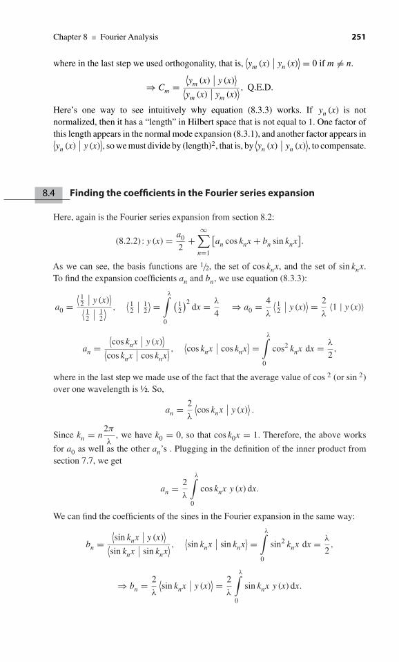
Chapter 8 ■ Fourier Analysis 251
where in the last step we used orthogonality, that is,⟨ym (x)
∣∣ yn (x)⟩ = 0 if m �= n.
⇒ Cm =⟨ym (x)
∣∣ y (x)⟩⟨
ym (x)∣∣ ym (x)
⟩ , Q.E.D.
Here’s one way to see intuitively why equation (8.3.3) works. If yn (x) is notnormalized, then it has a “length” in Hilbert space that is not equal to 1. One factor ofthis length appears in the normal mode expansion (8.3.1), and another factor appears in⟨yn (x)
∣∣ y (x)⟩, so we must divide by (length)2, that is, by
⟨yn (x)
∣∣ yn (x)⟩, to compensate.
8.4 Finding the coefficients in the Fourier series expansion
Here, again is the Fourier series expansion from section 8.2:
(8.2.2) : y (x) = a0
2+
∞∑n=1
[an cos knx + bn sin knx
].
As we can see, the basis functions are 1/2, the set of cos knx, and the set of sin knx.To find the expansion coefficients an and bn, we use equation (8.3.3):
a0 =⟨ 1
2
∣∣ y (x)⟩⟨ 1
2
∣∣ 12
⟩ ,⟨ 1
2
∣∣ 12
⟩ =λ∫
0
( 12
)2dx = λ
4⇒ a0 = 4
λ
⟨ 12
∣∣ y (x)⟩ = 2
λ〈1 | y (x)〉
an =⟨cos knx
∣∣ y (x)⟩⟨
cos knx∣∣ cos knx
⟩ , ⟨cos knx
∣∣ cos knx⟩ =
λ∫0
cos2 knx dx = λ
2,
where in the last step we made use of the fact that the average value of cos 2 (or sin 2)over one wavelength is ½. So,
an = 2
λ
⟨cos knx
∣∣ y (x)⟩.
Since kn = n2π
λ, we have k0 = 0, so that cos k0x = 1. Therefore, the above works
for a0 as well as the other an’s . Plugging in the definition of the inner product fromsection 7.7, we get
an = 2
λ
λ∫0
cos knx y (x) dx.
We can find the coefficients of the sines in the Fourier expansion in the same way:
bn =⟨sin knx
∣∣ y (x)⟩⟨
sin knx∣∣ sin knx
⟩ , ⟨sin knx
∣∣ sin knx⟩ =
λ∫0
sin2 knx dx = λ
2,
⇒ bn = 2
λ
⟨sin knx
∣∣ y (x)⟩ = 2
λ
λ∫0
sin knx y (x) dx.

252 Waves and Oscillations
Let’s collect these results:
y(x) = a0
2+
∞∑n=1
[an cos knx + bn sin knx
].
an = 2
λ
λ∫0
cos knx y (x) dx.
bn = 2
λ
λ∫0
sin knx y (x) dx.
kn = n2π
λ.
(8.4.1)
Fourier analysis for a function of x that has periodicity λ
Example: What is the Fourier series expansion for the square wave, shown as the leftgraph in figure 8.4.1?Solution: We can represent the square wave y(x) using the Fourier series expansionshown in the top line of equation (8.4.1). Let’s begin by calculating the an’s:
an = 2λ
λ∫0
cos knx y (x) dx = 2λ
⎡⎢⎣
λ/2∫0
cos knx (1) dx +λ∫
λ/2
cos knx (−1) dx
⎤⎥⎦
= 2λ
[1kn
sin knx
∣∣∣∣λ/2
0− 1
knsin knx
∣∣∣∣λλ/2
]
= 2λkn
[sin
(n
2π
λ
λ
2
)− sin 0 − sin
(n
2π
λλ
)+ sin
(n
2π
λ
λ
2
)]= 0.
Thus, all of the cosine coefficients in the Fourier expansion are zero. We could haveanticipated this based on symmetry: the square wave function is antisymmetric aboutthe point x = λ/2, whereas the cosine functions are all symmetrical about this point.
Figure 8.4.1 Left: Square wave. Middle: The square wave is antisymmetrical about x = λ/2,whereas the cosine is symmetrical. Right: Gray trace shows the sum of the first three non-zeroterms in the Fourier series expansion of the square wave.

Chapter 8 ■ Fourier Analysis 253
This is shown for the case n = 1 in the middle part of the figure. However, the sinefunctions do have the required symmetry, so we can anticipate that the bn’s will benonzero:
bn = 2λ
λ∫0
sin knx y (x) dx = 2λ
⎡⎢⎣
λ/2∫0
sin knx (1) dx +λ∫
λ/2
sin knx (−1) dx
⎤⎥⎦
= 2λ
[− 1
kncos knx
∣∣∣∣λ/2
0+ 1
kncos knx
∣∣∣∣λλ/2
]
= 2λkn
[− cos
(n
2π
λ
λ
2
)+ cos 0 + cos
(n
2π
λλ
)− cos
(n
2π
λ
λ
2
)]
= 2
λ n2π
λ
[− cos nπ + 1 + cos n2π − cos nπ ] = 2nπ
[1 − cos nπ ] .
If n is odd, then bn = 4nπ
, while if n is even then bn = 0. Plugging these results into the
top line of equation (8.4.1), we obtain
y (x) = 4π
(sin
2π
λ+ 1
3sin
3 · 2π
λ+ · · ·
)(8.4.2)
Fourier expansion for a square wave.
As you can see, each succeeding term is smaller (because of the factor 1/n). The rightgraph in figure 8.4.1 shows the sum of the first three terms. You can perhaps see howthe series begins to approximate the square wave. The approximation becomes betteras more terms are added.
Self-test (answer below3): Use symmetry arguments to explain why all the sines witheven n have zero coefficients.
You can show in problem 8.2 that an alternate version to equation (8.4.1) for theFourier series expansion is
y (x) = a0
2+
∞∑n=1
An cos(knx + ϕn
), (8.4.3)
where An =√
a2n + b2
n and ϕn = tan−1
(−bn
an
). This is the version used for
figure (8.1.1).We can also use Fourier analysis for a function of t. In fact, this is much more
common than using it for functions of x. Everything works in exactly the same way.The periodicity in x is replaced by the periodicity in t: λ → T . The wave number is
3. Although these terms are antisymmetrical about x = λ/2, they are also antisymmetrical aboutx = λ/4, whereas the square wave is symmetrical about this point.

254 Waves and Oscillations
replaced by the angular frequency: kn = n2π
λ→ ωn = n
2π
T. With these substitutions,
equation (8.4.1) becomes
y(t) = a0
2+
∞∑n=1
[an cos ωnt + bn sin ωnt
].
an = 2
T
λ∫0
cos ωnt y (t) dt.
bn = 2
T
λ∫0
sin ωnt y (t) dt.
ωn = n2π
T.
(8.4.4)
Fourier analysis for a function of t that has periodicity T
The version of equation (8.4.3) for functions of time is
y (t) = a0
2+
∞∑n=1
An cos(ωnt + ϕn
). (8.4.5)
8.5 Fourier Transforms and the meaning of negative frequency
Complex exponential version of Fourier analysis
In problem 8.3, you will show that the Fourier expansion can be written in termsof complex exponentials, rather than sines and cosines. You will show that wecan write
y(x) =∞∑
n=−∞Cneikn x, where Cn = 1
λ
λ∫0
y(x) e−iknxdx. (8.5.1)
You will also show that, although the Cn’s are complex, there is always cancellationof the imaginary part of the term n = m with the term n = −m, so that there is no needto take the real part of the summation to get y (x). One can show that the Cn ’s in thisexpansion are related to the an’s and bn’s in the sine/cosine expansion:
Cn = 1
2
(an − ibn
)and C−n = 1
2
(an + ibn
). (8.5.2)
This means for example, that for a case where C−n = Cn, we have bn = 0, that is, apure cosine term, while if C−n = −Cn, then we have an = 0, that is, a pure sine term.From equation (8.5.2), we can see that we must always have
∣∣C−n
∣∣ = ∣∣Cn
∣∣.

Chapter 8 ■ Fourier Analysis 255
Fourier transforms
If we take the limit λ → ∞, then the function y (x) is no longer truly periodic. However,
we can still express it as an infinite sum of sinusoids. Since kn = n2π
λ, as we increase λ
the kn’s get closer together. In the limit λ → ∞, the spacing between the kn’s becomesinfinitesimal. Now, instead of associating each Cn with a kn, it is more helpful to think ofa continuous function C(k). By convention, this is instead called Y (k). In problem 8.4,you can show that in the limit λ → ∞, equation (8.5.1) becomes
y(x) = 1√2π
∞∫−∞
Y (k)eikxdk, where Y (k) = 1√2π
∞∫−∞
y(x)e−ikxdx (8.5.3)
Fourier Transforms for a function of x
Y (k), which represents the Fourier amplitude as a function of k, is called the “FourierTransform” of y (x). At first, this might appear intimidating, but remember that anintegral is just an infinite sum, so that we are still expressing y (x) as a sum of thesinusoids eikx, each weighted by the factor Y (k).
It is easy to adapt this for functions of time: ω = 2π
Tplays the role of k = 2π
λ, so
that we can express any function of time y (t)as a weighted sum of the sinusoids eiωt :
y(t) = 1√2π
∞∫−∞
Y (ω)eiωtdω, where Y (ω) = 1√2π
∞∫−∞
y(t)e−iω tdt. (8.5.4)
Fourier Transforms for a function of t
Example: Fourier transform of a Gaussian. The Gaussian function is quite importantin several different contexts. It is defined as
y(t) = Ae−(t−t0)2/2σ 2, (8.5.5)
a bell-shaped curved centered on t0, as shown in figure 8.5.1a. For simplicity, let’sexamine the case t0 = 0, so that
y(t) = Ae−t2/2σ 2. (8.5.6)
Your turn: Verify that y(t) falls to A / 2 at t = ±σ
√−2 ln 1
2 = ±1.18 σ , so that the FullWidth at Half Maximum (FWHM) is 2.35 σ .
Using equation (8.5.4), we see that the Fourier transform of equation (8.5.6) is
Y (ω) = 1√2π
∞∫−∞
Ae−t2/2σ 2e−iω tdt. (8.5.7)
continued

256 Waves and Oscillations
Figure 8.5.1 a: The Gaussian. b: A Gaussian centered on t = 0 and its Fourier transform.The width (in time) of the y(t) Gaussian is inversely proportional to the width (in ω) ofthe Y (ω) Gaussian. Therefore a broad range of frequencies is needed to synthesize anarrow pulse.
This is a standard definite integral, which you can look up in a table (or evaluate with asymbolic calculus program):
∞∫−∞
e−(ax2+bx+c
)dx =
√π
ae(b2−4ac
)/4a. (8.5.8)
In our case, x → t, a → 1
2σ 2 , b → iω, and c → 0, so
Y (ω) = A√2π
√2πσ 2e−ω2/
(2/σ 2
)= Aσe−ω2/
(2/σ 2
).
We see that this has the same form as equation (8.5.6), that is, that the Fourier transformof a Gaussian function of time y (t) is a Gaussian function of angular frequency, Y (ω).
The FWHM of y (t) is 2.35 σ , so the FWHM of Y (ω) is 2.351σ
, as shown in figure 8.5.1b.
Thus, we arrive at a quite important conclusion: to Fourier synthesize a very narrowGaussian (one with a very small FWHM), we need a very broad range of frequencies (i.e.,a Gaussian Y (ω) with a very large FWHM).4 This conclusion holds in general: to Fouriersynthesize a function y (t) with variations on time scales as short as t, we must use
Fourier components covering a range of angular frequencies that is of order1t
.
4. As you can show in problem 8.18, this leads directly to the Heisenberg uncertainty principle.

Chapter 8 ■ Fourier Analysis 257
Meaning of the negative frequencies in the Fourier transform
The integral in equation (8.5.4) which represents the Fourier synthesis of y (t), y(t) =1√2π
∞∫−∞
Y (ω)eiω tdω, includes both positive and negative angular frequencies. Let’s
consider a particular positive angular frequency ω0. We can see that for each such afrequency in the integral, there is a corresponding negative frequency -ω0. Since theintegral is an infinite sum, the contributions at these frequencies are added together aspart of the integral: Y
(ω0
)eiω0 t + Y
(−ω0
)e−iω0 t . This sum must be real, since y (t)
is real, and this imposes a restriction on the relationship between Y(ω0
)and Y
(−ω0
),
as we explore below.The function eiω0t represents a vector of length 1 rotating counterclockwise in the
complex plane, while for e−iω0t the vector rotates clockwise, as shown in the top partof figure 8.5.2. If we add them together, then the imaginary part of e−iω0t cancels theimaginary part of eiω0t , leaving only a real function: eiω0 t + e−iω0 t = 2 cos ω0t. Ofcourse, we could multiply both by any real number, and still get cancellation of theimaginary parts: Aeiω0 t + Ae−iω0 t = 2A cos ω0t. Finally, we can add a positive phaseshift to the eiω0tand a negative phase shift of equal magnitude to the e−iω0t , and stillget cancellation of the imaginary parts:
Aei(ω0 t+ϕ) + Ae−i(ω0 t+ϕ) = 2A cos(ω0t + ϕ
), (8.5.9)
as shown in the bottom part of figure 8.5.2. This is the only way to get such cancellation.Applying these ideas to the sum Y
(ω0
)eiω0 t + Y
(−ω0
)e−iω0 t which is part of the
Fourier integral, we see that if we express Y(ω0
)in the form Y
(ω0
) = Aeiϕ , then we
Figure 8.5.2 Top: The imaginaryparts of two counter-rotating
complex plane vectors can cancelonly if the angular frequencies are
equal and the magnitudes areequal. Bottom: The phase factors
ϕ must be of equal magnitude andopposite sign for the imaginary
parts to cancel.
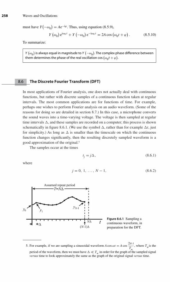
258 Waves and Oscillations
must have Y(−ω0
) = Ae−iϕ . Thus, using equation (8.5.9),
Y(ω0
)eiω0 t + Y
(−ω0
)e−iω0 t = 2A cos
(ω0t + ϕ
). (8.5.10)
To summarize:
Y(ω0
)is always equal in magnitude to Y
(−ω0
). The complex phase difference between
them determines the phase of the real oscillation cos(ω0t + ϕ
).
8.6 The Discrete Fourier Transform (DFT)
In most applications of Fourier analysis, one does not actually deal with continuousfunctions, but rather with discrete samples of a continuous function taken at regularintervals. The most common applications are for functions of time. For example,perhaps one wishes to perform Fourier analysis on an audio waveform. (Some of thereasons for doing so are detailed in section 8.7.) In this case, a microphone convertsthe sound waves into a time-varying voltage. The voltage is then sampled at regulartime intervals , and these samples are recorded on a computer; this process is shownschematically in figure 8.6.1. (We use the symbol , rather than for example t, justfor simplicity.) As long as is smaller than the timescale on which the continuousfunction changes significantly, then the resulting discretely sampled waveform is agood approximation of the original.5
The samples occur at the times
tj = j, (8.6.1)
where
j = 0, 1, . . . , N − 1, (8.6.2)
Figure 8.6.1 Sampling acontinuous waveform, inpreparation for the DFT.
5. For example, if we are sampling a sinusoidal waveform A cos ωt = A cos2π t
Tw, where Twis the
period of the waveform, then we must have � Tw in order for the graph of the sampled signalversus time to look approximately the same as the graph of the original signal versus time.

Chapter 8 ■ Fourier Analysis 259
and N is the number of samples. The result is a set of N data points: y(t0),
y(t1), . . . , y
(tN−1
). (In the example of the audio waveform, y would be the voltage.)
How can we represent this dataset in angular frequency space (the equivalent of k-spacefor functions of t), using ideas of Fourier analysis? In other words, how can we findthe “Fourier spectrum” of the dataset?
The algorithm used in such a situation is called the Discrete Fourier Transform(DFT). It assumes that the function has a periodicity T = N. However, most oftenthe continuous function that is being sampled (such as an audio waveform) does notactually have this periodicity, since N and are ordinarily determined by the hardwareand software used for data acquisition, rather than being determined by the systembeing examined.6 This assumption that the DFT algorithm makes about the periodicitycan cause serious inaccuracies in the Fourier transform that it calculates, particularlybecause the data point at the end of the set is usually at a different y-value than thedata point at the beginning. Thus, the assumed repeating function has a sharp step atthe beginning of each period. This would lead to spurious high-frequency peaks in theFourier spectrum. To avoid this, the input function is usually multiplied by a “window-ing function,” as shown in figure 8.6.2, forcing the start and end points to zero.Althoughthis windowing procedure does introduce some distortions into the Fourier spectrum,the benefits of eliminating the sharp step at the beginning of the period outweigh thesedrawbacks. You can explore the windowing operation more in problem 8.16.
Because the algorithm assumes a periodicity of T = N (equal to the measure-ment time), the lowest angular frequency in the Fourier spectrum is
ω1 = 2π
N, (8.6.2)
and the higher angular frequencies are integer multiples of this:
ωn = nω1 = n2π
N, where T = N is the total measurement time (8.6.3)
Figure 8.6.2 Because the DFT assumes the function has periodicity T , problems occur if (as isusually the case) the beginning and ending values of the sampled waveform (left) are notequal; this causes a sharp step in the assumed waveform. To avoid this problem, the sampledinput waveform (left) is multiplied by a windowing function (center) to produce a waveform(right) that goes to zero at the beginning and end of the time interval T . This example showsthe “Hanning window”, one of the most common windowing functions; it is simply an offsetcosine.
6. For example, if one is recording a vocalist singing a note at 440.3 Hz, corresponding to a periodof 2.271 ms, it is unlikely that the equipment used to make the recording will record for a timecorresponding to an exact multiple of 2.271 ms.
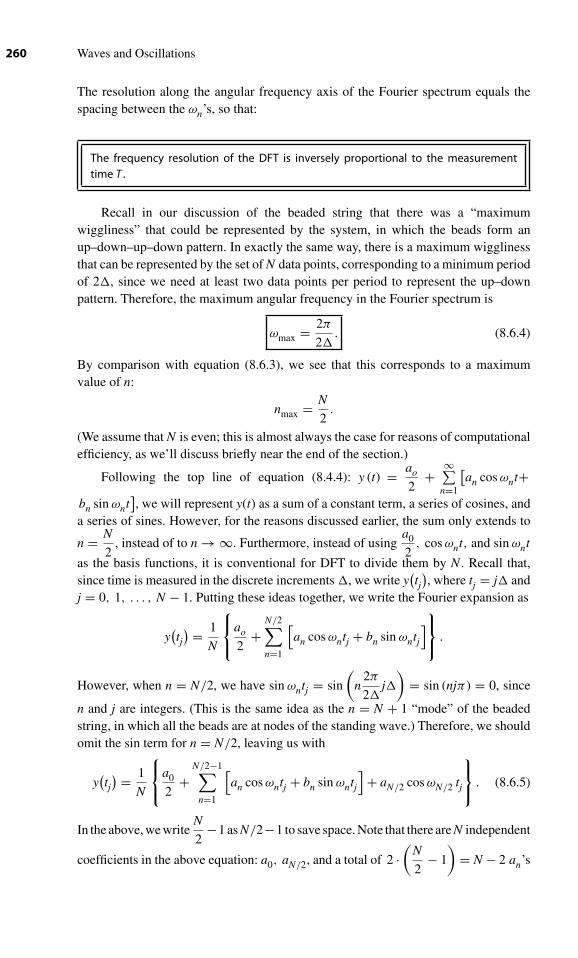
260 Waves and Oscillations
The resolution along the angular frequency axis of the Fourier spectrum equals thespacing between the ωn’s, so that:
The frequency resolution of the DFT is inversely proportional to the measurementtime T .
Recall in our discussion of the beaded string that there was a “maximumwiggliness” that could be represented by the system, in which the beads form anup–down–up–down pattern. In exactly the same way, there is a maximum wigglinessthat can be represented by the set of N data points, corresponding to a minimum periodof 2, since we need at least two data points per period to represent the up–downpattern. Therefore, the maximum angular frequency in the Fourier spectrum is
ωmax = 2π
2. (8.6.4)
By comparison with equation (8.6.3), we see that this corresponds to a maximumvalue of n:
nmax = N
2.
(We assume that N is even; this is almost always the case for reasons of computationalefficiency, as we’ll discuss briefly near the end of the section.)
Following the top line of equation (8.4.4): y (t) = ao
2+
∞∑n=1
[an cos ωnt+
bn sin ωnt], we will represent y(t) as a sum of a constant term, a series of cosines, and
a series of sines. However, for the reasons discussed earlier, the sum only extends to
n = N
2, instead of to n → ∞. Furthermore, instead of using
a0
2, cos ωnt, and sin ωnt
as the basis functions, it is conventional for DFT to divide them by N . Recall that,since time is measured in the discrete increments , we write y
(tj), where tj = j and
j = 0, 1, . . . , N − 1. Putting these ideas together, we write the Fourier expansion as
y(tj) = 1
N
⎧⎨⎩ao
2+
N/2∑n=1
[an cos ωntj + bn sin ωntj
]⎫⎬⎭ .
However, when n = N/2, we have sin ωntj = sin
(n
2π
2j
)= sin (njπ) = 0, since
n and j are integers. (This is the same idea as the n = N + 1 “mode” of the beadedstring, in which all the beads are at nodes of the standing wave.) Therefore, we shouldomit the sin term for n = N/2, leaving us with
y(tj) = 1
N
⎧⎨⎩a0
2+
N/2−1∑n=1
[an cos ωntj + bn sin ωntj
]+ aN/2 cos ωN/2 tj
⎫⎬⎭ . (8.6.5)
In the above, we writeN
2−1 as N/2−1 to save space. Note that there are N independent
coefficients in the above equation: a0, aN/2, and a total of 2 ·(
N
2− 1
)= N − 2 an’s

Chapter 8 ■ Fourier Analysis 261
and bn’s in the summation. Given that we started with N independent values of y, it islogical that we should have N independent coefficients in the Fourier expansion.
It is customary to write the DFT using complex exponentials instead of sines andcosines. The expansions for cosine and sine in terms of complex exponentials are:
cos ωnt = eiωnt + e−iωnt
2and sin ωnt = eiωnt − e−iωnt
2i= −i
eiωnt − e−iωnt
2.
Therefore, we can write equation (8.6.5) as
y(tj)= 1
N
⎧⎨⎩a0
2+
N/2−1∑n=1
[an
eiωntj +e−iωntj
2−ibn
eiωntj −e−iωntj
2
]+aN/2cosωN/2 tj
⎫⎬⎭.
(Because the cos ωN/2 t term has no accompanying sin term, we choose not to expressit as a complex exponential.)
Your turn: Show that, by defining
Cn ≡ 12
(an − ibn
)and C−n ≡ 1
2
(an + ibn
), (8.6.6)
we can rewrite the above equation as
y(tj) = 1
N
⎧⎨⎩a0
2+
N/2−1∑n=1
[Cneiωntj + C−ne−iωntj
]+ aN/2 cos ωN/2 tj
⎫⎬⎭ .
Because of equation (8.6.3): ωn = n2π
N, we have that −ωn = ω−n. Using this, we
can compress the above equation to
y(tj) = 1
N
⎧⎨⎩
N/2−1∑n=−(N/2−1)
Cneiωntj + aN/2 cos ωN/2 tj
⎫⎬⎭ , (8.6.7)
where we have defined b0 ≡ 0, so that the entry in the sum for n = 0 is C0eiω0tj =a0
2e0 = a0
2.
For all values of n other than N /2, the basis functions in this expansion are∣∣∣yn
(tj)⟩ ≡ eiωntj
N. To find the coefficients Cn, we can use the version of equation (8.3.3):
Cn =⟨yn (x)
∣∣ y (x)⟩⟨
yn (x)∣∣ yn (x)
⟩ that would be appropriate for a function of time, that is,
Cn =⟨yn
(tj) ∣∣ y
(tj)⟩
⟨yn
(tj) ∣∣ yn
(tj)⟩ .
Because we have a discrete set of data y(tj), the inner products are taken in the same
way as we would for a beaded string. For example,
⟨yn
(tj) ∣∣∣yn
(tj)⟩=N−1∑
j=0
(eiωntj
N
)∗(eiωntj
N
)=
N−1∑j=0
(e−iωntj
N
)(eiωntj
N
)=
N−1∑j=0
1
N2= 1
N,

262 Waves and Oscillations
where the last step follows because there are N identical terms in the sum. Therefore,the coefficients Cn are given by
Cn = N⟨yn
(tj) ∣∣ y
(tj)⟩ = N
N−1∑j=0
e−iωntj
Ny(tj)
⇒ Cn =N−1∑j=0
e−iωntj y(tj). (8.6.8)
Similarly, to find aN/2, we use
aN/2 =⟨yN/2
(tj) ∣∣ y
(tj)⟩
⟨yN/2
(tj) ∣∣ yN/2
(tj)⟩ , (8.6.9)
where∣∣yN/2
(tj)⟩ = cos ωN/2tj
N. The denominator is
⟨yN/2
(tj) ∣∣ yN/2
(tj)⟩ =
N−1∑j=0
cos2 ωN/2tjN2
.
Recall from equations (8.6.3) and (8.6.1) that ωn = n2π
Nand tj = j, so that ωN/2 tj =
π j. Plugging this in gives
⟨yN/2
(tj) ∣∣ yN/2
(tj)⟩ =
N−1∑j=0
cos2 π j
N2=
N−1∑j=0
(±1)2
N2= 1
N.
Therefore, equation (8.6.9) becomes
aN/2 = N⟨yN/2
(tj) ∣∣ y
(tj)⟩ = N
N−1∑j=0
cos ωN/2tjN
y(tj) ⇒
aN/2 = NN−1∑j=0
cos π j
Ny(tj). (8.6.10)
Since
e−iωN/2 tj = e−iπ j = cos (−π j) + i sin (−π j) = cos π j,
we can write equation (8.6.10) as
aN/2 =N−1∑j=0
e−iωN/2 tj y(tj).
Since this has the same format as equation (8.6.8), we can write
aN/2 cos ωN/2 tj = CN/2 cos ωN/2 tj = CN/2 cos π j. (8.6.11)
Since
eiωN/2 tj = eiπ j = cos π j + i sin π j = cos π j,

Chapter 8 ■ Fourier Analysis 263
we can write equation (8.6.11) as
aN/2 cos ωN/2 tj = CN/2eiωN/2tj .
Now, we insert this into equation (8.6.7) to give
y(tj) = 1
N
⎧⎨⎩
N/2−1∑n=−(N/2−1)
Cneiωntj + CN/2eiωN/2tj
⎫⎬⎭ . (8.6.12)
In the above, n ranges from −(
N
2− 1
)to
(N
2− 1
). However, it is conventional for
DFT to change this range. Recall from equations (8.6.3) and (8.6.1) that ωn = n2π
N
and tj = j, so ωn tj = nj
N2π . Therefore,
eiωn+N tj = ei (n+N)jN 2π = ei N j
N 2πei n jN 2π = eij2πei n j
N 2π = ei n jN 2π = eiωn tj .
This means that we can add N to the index n for any of the terms of the sum in equation(8.6.12) without changing anything. We will do this for all the negative values of n, sothat, for example,
n = −(
N
2− 1
)+N−−→ N
2+ 1 and n = −1
+N−−→ N − 1. (8.6.13)
Using this, equation (8.6.12) becomes
y(tj) = 1
N
⎧⎨⎩
N/2−1∑n=0
Cneiωntj +N−1∑
n=N/2+1
Cneiωntj + CN/2eiωN/2tj
⎫⎬⎭
⇒ y(tj) =
N−1∑n=0
Cneiωntj , (8.6.14)
where equation (8.6.8):
Cn =N−1∑j=0
y(tj)
e−iωntj .
Equation (8.6.8) for the coefficients is called the Discrete Fourier Transform (DFT),while equation (8.6.14), which describes the Fourier synthesis of y
(tj), is called the
Inverse Discrete Fourier Transform (IDFT).In equation (8.6.14), the term for n = 0 is the constant term, and the terms for n = 1
to n = N
2− 1 correspond to the positive frequencies ω1 to ωN/2 − 1. However, because
of the transformation (8.6.13), the terms from n = N
2+ 1 to n = N − 1 correspond to
the negative frequencies ω−(N/2 − 1) to ω−1. Finally, the term for n = N/2 is derivedfrom a sum of positive and negative frequency terms. Although this is the conventionalsequence for the DFT, it is not very intuitive, because the highest frequency componentsare those near n = N/2, while the components near n = N − 1 correspond to low

264 Waves and Oscillations
Figure 8.6.3 a: A function y sampled at 1000 times tj . b: The magnitude of the DFT for thisfunction. Note the symmetry about n = N/2. If one is only interested in the magnitude of the
Fourier spectrum, then the points from n = N
2+ 1 to n = N − 1 can be ignored.
frequencies (as do the components near n = 0). As with the Fourier Transform (seesection 8.5), there is no need to take the real part of anything in any of the abovediscussions. There is therefore the same condition that the magnitude of the Cn for apositive frequency must equal the magnitude of the Cn for the corresponding negativefrequency, so that these terms can combine to cancel the imaginary parts. Because ofthe transformation (8.6.13), this means that∣∣Cn
∣∣ = ∣∣CN−n
∣∣ . (8.6.15)
Figure 8.6.3a shows a sequence of N = 1,000 data points as a function of time,in which there is no obvious pattern. Figure 8.6.3b shows the magnitude of the DFTof this data (i.e.,
∣∣Cn
∣∣as a function of n) , with the conventional sequence of n values,that is, the sequence of equation (8.6.14). The pattern is symmetrical about the pointn = N/2 = 500. In fact, if one is only interested in the magnitudes
∣∣Cn
∣∣, which is often
the case, then the points from n = N
2+ 1 to n = N − 1 can be ignored, and one can
focus just on the values for n = 0 to n = N
2.
It would appear from equations (8.6.14) and (8.6.8) that computing the DFT wouldtake a number of steps proportional to N2, since there are N different coefficients Cn,and to compute each of these one must do the sum (8.6.8) which has N entries. However,if N = 2m, where m is an integer, then one can use a computer algorithm called the“Fast Fourier Transform” (FFT) to compute the DFT, and this takes a number ofsteps that is only proportional to N log N , a tremendous improvement. You may have

Chapter 8 ■ Fourier Analysis 265
heard of research on quantum computers, in which data is represented by quantumsuperpositions. Such computers have not yet been fully realized, but one can showthat they could be used to compute DFTs with a number of steps proportional only to(log N)2, a tremendous further improvement.
Because the DFT is of enormous scientific and commercial importance, a greatdeal has been written about it. To learn more, you might begin with the classictext “Numerical Recipes”,7 although you should beware that it follows the unusual
convention of usinge−iωntj
Nas the basis functions for the Fourier synthesis of y, rather
than usingeiωntj
Nas do most authors and as we have done above. The text by Julius O.
Smith8 is also very approachable, and includes reviews of all the necessary math.
8.7 Some applications of Fourier Analysis
Fourier analysis is so widespread in science and engineering that there are applicationsin virtually every subfield. In this section, we explore two of them briefly.
Sonograms and whale calls. For scientists studying birds and animals, it canbe very helpful to have a visual representation of the characteristic calls made by aparticular species. A microphone converts the sound into a time-varying voltage. Thevoltage is sampled at regular time intervals for a measurement period T . The DFTfor this dataset is calculated, and then the process is immediately repeated.
Self-test (answer below9): (This is a hard self-test the first time you encounter it. So,don’t spend too long on it before looking at the answer.) A scientist wishes to createa DFT of the sound of a whale call. She wants to make a plot of
∣∣Cn
∣∣ versus angularfrequency, with the angular frequency ranging from 0 to 2π · (1,000 Hz), and with aresolution in angular frequency of 2π · (10 Hz). What values of the sampling interval
and the measurement period T should she use?
A “sonogram” is a series of DFT plots at successive times, with∣∣Cn
∣∣indicated bya gray scale, frequency f = ω/2π on the vertical scale, and time on the horizontalscale. (The time steps on the horizontal axis are equal to T , the time needed to collectenough data for a DFT.) Figure 8.7.1a shows the sonogram for the call of a right whale,showing that the call has three simultaneous frequency components, at about 250, 550,
7. Numerical Recipes: The Art of Scientific Computing, 3rd Ed., by W.H. Press, S. A. Teukolsky,W. T. Vetterling, and B. P. Flannery, Cambridge University Press, Cambridge, 2007.
8. Mathematics of the Discrete Fourier Transform with Audio Applications, 2nd Ed., by Julius O.Smith III, BookSurge Publishing, 2007.
9. From equation (8.6.4), we have ωmax = 2π
2, so we need
1
2= 1, 000 Hz ⇔ = 0.5 ms.
Equation (8.6.3) states ωn = n2π
N, so the angular frequency resolution is
2π
N= 2π
T. Setting
this equal to 2π · (10 Hz) gives T = 0.1 s.

266 Waves and Oscillations
Figure 8.7.1 a: Sonogram of a Right whale. b: Sonograms for four different species of whale.Note the different time and frequency scales. Darker shades of gray darker gray indicate larger∣∣Cn
∣∣. Images courtesy of and © Prof. Christopher W. Clark, Cornell University.
and 850 Hz. This would be almost impossible to tell from the graph of voltage versustime from the microphone. Figure 8.7.1b compares the calls from four different speciesof whales.
There are fewer than 400 right whales remaining in the world. Although thesewhales were heavily hunted in the past, collisions with ships account for many currentfatalities. Scientists are working to protect these whales using underwater microphoneson buoys to detect their calls, then warning ships away from possible collisions. It isessential to distinguish the calls of the right whales from other sounds in the ocean,to avoid false positives. The current generation of detection buoys uses relativelysimple techniques in an effort to select out the most significant signals, but the resultsleave much to be desired. Scientists are hopeful that a future generation of buoys,with computerized analysis of sonograms, will lead to more accurate detection. Youcan learn more about this effort, including viewing a live map of the most recent rightwhale detections, and listening to the calls, by visiting the links listed under this sectionon the web page for this text.
JPEG image compression. According to the old saying, “A picture is wortha thousand words.” In fact, it takes 11 kB(kilobytes) to store 1,000 words (at leastin the format used by my word processor), but it takes 9 MB (megabytes) to storea reasonably high resolution (three megapixel) image if it is not compressed first.Although storage has become inexpensive, the transmission of data is still a bottleneckin many circumstances, so it is important to reduce the amount of data needed torepresent photographs and other images. After compression by the jpeg algorithm, thesame photo can be reduced to about 1 MB in size with no loss of quality that is visibleto the eye. In fact, it can be compressed to about 100 kB with only a little loss ofquality, unless one examines a magnified version. So, a more accurate version of thesaying might be, “A picture is worth at least 10,000 words.”
There are several image compression algorithms in wide use. The jpeg (“jointphotographic experts group”) method works especially well on photos, but canintroduce significant artifacts into schematic diagrams and other figures with sharp

Chapter 8 ■ Fourier Analysis 267
edges and high contrast. In the jpeg method, the image is divided into squares of8 × 8 pixels. The colors are represented by three numbers for each pixel, with onenumber indicating the overall brightness and the other two indicating hue. Becausethese numbers are functions of x and y (rather than of time), the Fourier transform isin terms of wavenumbers (rather than angular frequencies). Each of the three sets ofcolor numbers for each 8 × 8 square is run through a version of the DFT called the“Discrete Cosine Transform” (DCT). This uses only cosines as basis functions, ratherthan both sines and cosines. However, the wavenumber spacing between the cosinesof the DCT is half that of the wavenumber spacing for DFT, so that the total number ofbasis functions is the same. (Recall that, for normal mode analysis of a beaded string
we use only sines, with kn = nπ
L, whereas for Fourier analysis of a function of x we
use both sines and cosines, but with twice the wavenumber spacing: kn = n2π
λ.) In
addition to the difference in basis functions, the DCT used for jpeg is a two-dimensionaltransform; this is essentially a product of transforms in the x- and y-directions.
The advantage for jpeg of expressing the information in the 8 × 8 square as asum of cosines is that the eye is less sensitive to the high wavenumber (i.e., shortwavelength) components, and usually these components are smaller than the lowwavelength components. Therefore, after using the DCT to compute the coefficientsin the sum of cosines, the higher wavenumber coefficients can be represented withvery low accuracy, or even set to zero, with little perceptible change in the imageafter the inverse transformation (to go back from the cosines to the real-spacecolors of the pixels) has been applied. This is how the jpeg algorithm achievesmuch of its compression, although significant compression is also obtained byother steps.
Concept and skill inventory for chapter 8
After reading this chapter, you should fully understand the following
terms:
Basis function (8.2)Complete basis (8.2)Orthogonal functions (8.3)Fourier series expansion (8.4)Fourier transform (8.5)Negative frequency (8.5)Discrete Fourier Transform (DFT) (8.6)Sonogram (8.7)
You should understand the following connections:
Fourier analysis & normal mode analysis (8.2)The frequency resolution of the DFT & the measurement time (8.6)The maximum angular frequency of the DFT & the sampling interval (8.6)

268 Waves and Oscillations
You should understand the difference between:
Fourier series expansions & Fourier transforms (8.5)
You should be familiar with the following additional concepts:
The Fourier transform of a Gaussian is a Gaussian; the FWHMs are inverselyrelated (8.5)
You should be able to:
Express any periodic function as a weighted sum of sines and cosines (8.4)Use symmetry arguments to deduce which Fourier expansion coefficients are zero (8.4)Given a complete set of orthogonal basis functions, express any function as a weighted
sum of the basis functions, even if they aren’t normalized (8.3)Find the Fourier transform of a function that isn’t periodic (8.5)Calculate the DFT by hand for very small datasets (e.g., up to four points) (8.6)
Explain the meaning of the DFT terms from n = N
2+ 1 to n = N − 1 (8.6)
In addition to all of the above, you should be able to combine the concepts
you’ve learned to address new situations.
Problems
Note: Additional problems are available on the website for this text.
Instructors: Difficulty ratings for the problems, full solutions, and importantadditional support materials are available on the website.
8.1 Show that all the terms in the Fourier expansion (including sines, cosines,and the constant term) of y(x) are orthogonal to each other. There are fivecombinations you must test: sines versus sines, sines versus cosines, sinesversus constant, cosines versus cosines, and cosines versus constant.You may need the following integrals:
∫sin px sin qx dx = sin (p − q) x
2 (p − q)− sin (p + q) x
2 (p + q)p �= ±q
∫cos px cos qx dx = sin (p − q) x
2 (p − q)+ sin (p + q) x
2 (p + q)p �= ±q
∫sin px cos qx dx = − cos (p − q) x
2 (p − q)− cos (p + q) x
2 (p + q)
8.2 Show that an alternate version to equation (8.4.1) for the Fourier seriesexpansion is
y (x) = a0
2+
∞∑n=1
An cos(knx + ϕn
),

Chapter 8 ■ Fourier Analysis 269
where An =√
a2n + b2
n and ϕn = tan−1
(−bn
an
). (This is the version used
for figure 8.1.1.)8.3 The complex version of the Fourier expansion. Frequently, instead of
thinking of the Fourier expansion in terms of sines and cosines, it is moreconvenient to think of it in terms of complex exponentials. (a) Assume that
the set of complex exponentials eiknx, where kn = n2π
λand n ranges from
−∞ to +∞, forms a complete basis for functions y(x) with periodicity λ,so long as we allow the expansion coefficients to be complex. (It is reasonableto assume that this is a complete basis, since each exponential contains somecos character and some sin character, and since we can vary the balancebetween the sin and cos by varying the balance between real and imaginaryin the expansion coefficient.) This means that we can write
y(x) =∞∑
n=−∞Cneikn x.
Note: There is no “Re” in the above expression; this is intentional andcorrect.Show that the basis functions in this expansion are mutually orthogonal.Hint: Remember that for a Fourier expansion, the inner product is definedas an integral from 0 to λ. (b) Show that the expansion coefficients
are given by Cn = 1
λ
λ∫0
e−iknxy(x) dx. Hint: you may wish to refer to the
discussion of generic orthonormal function expansions with nonnormalizedbasis functions in section 8.3. (c) If y(x) is real (the usual case), then all theimaginary parts of the expansion above must somehow cancel out. Showin detail how this happens. Hint: Cancellation occurs between the term atn = m and the term at n = -m.
8.4 The Fourier transform. So far, we’ve discussed how any function withperiodicity λ can be expressed as a sum of sines and cosines with thesame periodicity (plus a constant term); the difference in the wavenumberk between the longest wavelength sinusoidal component and the next-to-
longest is given by k1 = 2π
λ. (In fact the difference between any two
“adjacent” (in k-space) sinusoidal components is k1.) It is also possible toexpress even nonperiodic functions in this way, so long as we allow thisspacing to become infinitesimal. In this problem, you’ll derive the equationswhich apply in this limit.
In problem 8.3, you can show that the complex exponential version ofFourier analysis is
y(x) =∞∑
n=−∞Cneiknx, (1)
where kn = n2π
λand Cn = 1
λ
λ∫0
e−iknxy (x) dx.

270 Waves and Oscillations
It should be fairly clear that, to evaluate the Cn’s, it is only necessary tointegrate over one period of y(x); as long as we use the same integrationinterval for all the Cn’s, we can choose whatever interval corresponding toone period that we like. In particular, it will make things look prettier if,instead of integrating from 0 to λ, we integrate from −λ/2 to λ/2, that is, wecould just as well write:
Cn = 1
λ
λ/2∫−λ/2
e−iknxy (x) dx. (2)
We can think of a nonperiodic y(x) as a periodic function with λ → ∞.According to the above equation, all the Cn’s appear to go to zero in thislimit, so we must proceed carefully. Although the Cn’s do get smaller, thenumber of them in any interval from k to k+ dk gets bigger, so the net resultwinds up still being OK, as you’ll show. As shown in the above equation(on the right), each Cn depends on the value of kn = nk1, so instead ofwriting them as Cn, we might write them as C(kn). In the limit λ → ∞, thespacing (in k-space) between the C’s becomes infinitesimal. In this limit, wecan write them as C(k) instead of C(kn). Unless something pathological ishappening, all the C’s in the interval k to k+ dk will have the same value, ifwe’re taking the limit dk → 0. A representative one of the C’s in this intervalwould have the value
C (k) = 1
λ
λ/2∫−λ/2
e−ik xy (x) dx. (3)
To form y(x) from these C’s, we must form an integral over k instead of thesum shown in (1). This integral (in the limit λ → ∞) would be given by
y(x) =∞∫
−∞(# of C’s in the interval k to k + dk) (value of a typical C(k)
in this range)eikx,
where the (value of a typical C(k) in this range) would be given by (3)
(a) Show that the (# of allowed C’s in the interval k to k+ dk) is given
byλ
2πdk. (This is almost trivial.)
(b) Use this result to show that
y(x) = 1√2π
∞∫−∞
Y (k)eikxdk, where Y (k) = 1√2π
∞∫−∞
y(x)e−ikxdx.
Note: Y (k) and y(x) are referred to as a “Fourier transform pair.” They containthe same information, but one version, y(x), is expressed in regular space,while the other, Y (k), is expressed in k-space.
8.5 What is the Fourier series representation for the triangle wave, shown infigure 8.P.1?
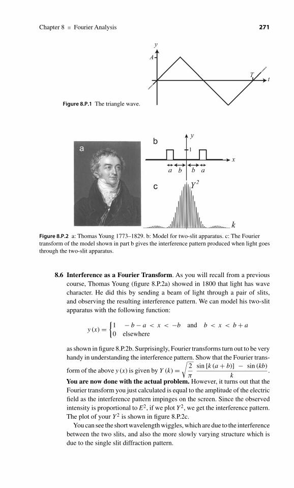
Chapter 8 ■ Fourier Analysis 271
Figure 8.P.1 The triangle wave.
Figure 8.P.2 a: Thomas Young 1773–1829. b: Model for two-slit apparatus. c: The Fouriertransform of the model shown in part b gives the interference pattern produced when light goesthrough the two-slit apparatus.
8.6 Interference as a Fourier Transform. As you will recall from a previouscourse, Thomas Young (figure 8.P.2a) showed in 1800 that light has wavecharacter. He did this by sending a beam of light through a pair of slits,and observing the resulting interference pattern. We can model his two-slitapparatus with the following function:
y (x) ={
1 − b − a < x < −b and b < x < b + a0 elsewhere
as shown in figure 8.P.2b. Surprisingly, Fourier transforms turn out to be veryhandy in understanding the interference pattern. Show that the Fourier trans-
form of the above y (x) is given by Y (k) =√
2
π
sin [k (a + b)] − sin (kb)
k.
You are now done with the actual problem. However, it turns out that theFourier transform you just calculated is equal to the amplitude of the electricfield as the interference pattern impinges on the screen. Since the observedintensity is proportional to E2, if we plot Y2, we get the interference pattern.The plot of your Y2 is shown in figure 8.P.2c.
You can see the short wavelength wiggles, which are due to the interferencebetween the two slits, and also the more slowly varying structure which isdue to the single slit diffraction pattern.

272 Waves and Oscillations
In fact, one can show that the Fourier transform of the “aperture function”always gives the amplitude of the electric field, so that the square of theFourier transform gives the interference pattern.
8.7. (a) Find the Fourier transform of y = Ae−a|x| , where a > 0.(b) Find the FWHM (full width at half maximum) of y, and set this
FWHM equal to W .(c) Express the FWHM of the Fourier transform of y in terms of W .
8.8. In problem 8.4, you showed that we can express any function y(x) in theform
y(x) = 1√2π
∞∫−∞
Y (k)eikxdk. (1)
You also showed that, if we write y(x) this way, then its “Fourier transform”Y (k) can be found by
Y (k) = 1√2π
∞∫−∞
y(x)e−ikxdx. (2)
The above equations are my favorite way of writing the Fourier transform,since they emphasize the symmetry between y(x) and Y (k). Althoughabout half the world uses the above way of writing the Fourier transform,unfortunately the other half uses a slightly different formulation. In thisversion, we instead express y(x) as
y(x) = 1
2π
∞∫−∞
Y (k)eikxdk. (3)
For this way of expressing y(x) , the expression for Y (k) (equation 2) needs tobe adjusted slightly to be correct. What would be the correct expression forY (k) to go with equation 3? Explain your answer thoroughly. Hint: Thereis almost no additional math required for this problem. It will probably helpyou to think in terms of basis functions/vectors in Hilbert space, althoughthere are other good ways to do this problem.
8.9 Time scaling of the Fourier transform. Consider a function y(t) withFourier transform Y (ω). The function y′ (t) = y (at) is the same as y(t),except that it is compressed by the factor a along the time axis. For example,if there is a peak in y(t) at t = 1s, and a = 2, then the same peak appears iny′ (t) = y (at) at t = 0.5 s. Assuming a > 0 show that the Fourier transform
of y′ (t) is Y ′ (ω) = 1
aY(ω
a
). (This means that Y ′ (ω) is expanded by the
factor a along the ω axis.)8.10 Fourier transform of the Dirac delta function
(a) Explain briefly why the Kronecker delta function has the propertythat it “picks out” the “matching” term in a series, that is,
∞∑n=−∞
f (n) δmn = f (m), where f is a function.

Chapter 8 ■ Fourier Analysis 273
(b) The Kronecker delta function only works for discrete variables, suchas n in the example above or kn for a finite-length string stretchedbetween two walls. However, it is often handy to have a similarfunction which works for continuous variables. This is called the“Dirac delta function,” and is written δ(x − a). It has the propertythat for x �= a, δ(x − a) = 0 (this is analogous to the Kroneckerdelta function). However, for x = a, δ(x − a) = "∞", where theinfinity is in quotes because the “extent” of the infinity is carefullydefined below. However, it is correct to picture the graph of δ (x − a)versus x as being zero everywhere except for an infinitely tall andinfinitely narrow spike at x = a. Here’s the final part of the definitionof the Dirac delta function: the height of the spike is the “rightamount of infinity” so that
∞∫−∞
f (x) δ (x − a) dx = f (a) ,
which is analogous to the equation in part a) of this problem, thatis, the Dirac delta function “picks out” the “matching” term in theintegral. Find the Fourier transform of the Dirac delta function forthe case a = 0.
(c) Now that you know the answer, explain how you might havepredicted it qualitatively based on the example “Fourier Transformof a Gaussian” in section 8.5.
(d) What is the “inverse Fourier transform” of δ(k − k0
)for the case
k0 = 0? (The “inverse Fourier transform” means the function y(x)whose Fourier transform is δ
(k − k0
).)
(e) When a (or k0) is not equal to zero, things are slightly morecomplicated, though in a philosophical sense they are still aboutthe same. What is the inverse Fourier transform of δ
(k − k0
)for k0
not necessarily equal to zero?(f) Now that you know the answer to the above, explain why it makes
qualitative sense.
8.11 More about the Dirac delta function. Read the first two parts of problem8.10. (You need not actually do them before you do this problem). In part b ofthat problem, you can show that the Fourier transform of δ (x) is 1/
√2π .This,
of course, means that the Fourier transform of δ (t) is also 1/√
2π . (a) Use
this as a starting point for this problem, and show that∞∫
−∞eiωt dω = 2πδ (t).
(b) Explain why, therefore,∞∫
−∞e−iωt dω = 2πδ (t).
8.12 The left column of figure 8.P.3 shows several different functions of time.The right column shows the magnitudes of the Fourier amplitudes for thesefunctions, though the order has been scrambled, for example plot g doesnot show the Fourier amplitudes for the function y (t) in part a. “Fourieramplitude” means the amplitude An in the Fourier expansion expressed

274 Waves and Oscillations
Figure 8.P.3 The left column shows various functions of time, with the same vertical andhorizontal scale for each plot. The right column shows the magnitude of the Fourier amplitudeas a function of ω, with the same horizontal scale for each plot. The insets for j and k showmagnified views of the low-ω region; the horizontal scale on the two insets is the same.Note that parts h and i each show just a single dot, near the top left.
as (8.4.5): y (t) = a0
2+
∞∑n=1
An cos(ωnx + ϕn
). The Fourier amplitudes are
plotted as a function of ω. Which entry from the right column goes witheach of the entries from the left column? Explain each of your choicesbriefly.

Chapter 8 ■ Fourier Analysis 275
8.13 Parseval’s theorem. We have seen that energy is proportional to the squareof amplitude. For example, the potential energy of a simple harmonicoscillator is 1
2 kA2. Therefore, it is reasonable to expect that the sums ofsquares of amplitudes in the time domain are proportional to the sums ofsquares of amplitudes in the frequency domain, since both sums should beproportional to the energy. (a) We begin with a simple illustration of this
idea. Let y (t) = A1 cos ω1t + A2 cos ω2t, where ω1 = 2π
Tand ω2 = 2ω1.
The sum of squares of amplitudes in the frequency domain would simplybe A2
1 + A22. To find the “sum of squares of amplitudes in the time domain,”
we must integrate:T∫0
[y (t)]2 dt. Show that this is proportional to A21 + A2
2.
(b) In part a, we considered Fourier synthesis of a periodic function, asdescribed in section 8.4. Now, we consider Fourier transforms. As you’llrecall from section 8.5, these involve complex exponentials. Therefore,instead of discussing the “sum of squares of amplitudes,” we discuss the“sum of squares of magnitudes.” Prove Parseval’s theorem, which states
that∞∫
−∞|y (t)|2 dt =
∞∫−∞
|Y (ω)|2 dω, where y (t)and Y (ω) are a Fourier
transform pair, as defined by (8.5.4). Hint: use the result of problem 8.11 ;since this is a mathematical result, you can interchange the symbols ω andt and it will still be correct.
8.14 State whether each of the following is true or false. If true, explain whybriefly. If false, explain why and provide a corrected version that is notsimply a negation of the original statement. Important: assume that y (t) is real.
(a) In the Fourier transform (8.5.4), the imaginary part of Y (ω) is justa mathematical convenience. We could just as well write
y(t) = 1√2π
∞∫−∞
Y (ω)eiω tdω,
where Y (ω) = Re
⎡⎣ 1√
2π
∞∫−∞
y(t)e−iω tdt
⎤⎦ .
(b) In the Fourier transform (8.5.4), the negative frequencies are just amathematical convenience. We could just as well write
y(t) = 2Re
⎡⎣ 1√
2π
∞∫0
Y (ω)eiω tdω
⎤⎦ ,
where Y (ω) = 1√2π
∞∫−∞
y(t)e−iω tdt.
8.15 Aliasing. We have discussed why the maximum angular frequency thatcan be represented by samples taken at time intervals spaced by is
ωN/2 = 2π
2= π
. (The corresponding frequency, fc = ωN/2
2πis called the
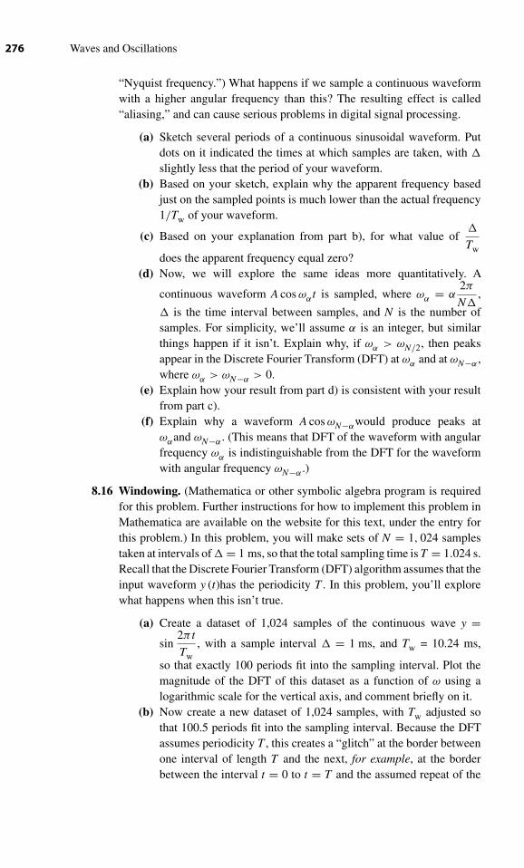
276 Waves and Oscillations
“Nyquist frequency.”) What happens if we sample a continuous waveformwith a higher angular frequency than this? The resulting effect is called“aliasing,” and can cause serious problems in digital signal processing.
(a) Sketch several periods of a continuous sinusoidal waveform. Putdots on it indicated the times at which samples are taken, with
slightly less that the period of your waveform.(b) Based on your sketch, explain why the apparent frequency based
just on the sampled points is much lower than the actual frequency1/Tw of your waveform.
(c) Based on your explanation from part b), for what value of
Twdoes the apparent frequency equal zero?
(d) Now, we will explore the same ideas more quantitatively. A
continuous waveform A cos ωαt is sampled, where ωα = α2π
N,
is the time interval between samples, and N is the number ofsamples. For simplicity, we’ll assume α is an integer, but similarthings happen if it isn’t. Explain why, if ωα > ωN/2, then peaksappear in the Discrete Fourier Transform (DFT) at ωα and at ωN−α ,where ωα > ωN−α > 0.
(e) Explain how your result from part d) is consistent with your resultfrom part c).
(f) Explain why a waveform A cos ωN−αwould produce peaks atωαand ωN−α . (This means that DFT of the waveform with angularfrequency ωα is indistinguishable from the DFT for the waveformwith angular frequency ωN−α .)
8.16 Windowing. (Mathematica or other symbolic algebra program is requiredfor this problem. Further instructions for how to implement this problem inMathematica are available on the website for this text, under the entry forthis problem.) In this problem, you will make sets of N = 1, 024 samplestaken at intervals of = 1 ms, so that the total sampling time is T = 1.024 s.Recall that the Discrete Fourier Transform (DFT) algorithm assumes that theinput waveform y (t)has the periodicity T . In this problem, you’ll explorewhat happens when this isn’t true.
(a) Create a dataset of 1,024 samples of the continuous wave y =sin
2π t
Tw, with a sample interval = 1 ms, and Tw = 10.24 ms,
so that exactly 100 periods fit into the sampling interval. Plot themagnitude of the DFT of this dataset as a function of ω using alogarithmic scale for the vertical axis, and comment briefly on it.
(b) Now create a new dataset of 1,024 samples, with Tw adjusted sothat 100.5 periods fit into the sampling interval. Because the DFTassumes periodicity T , this creates a “glitch” at the border betweenone interval of length T and the next, for example, at the borderbetween the interval t = 0 to t = T and the assumed repeat of the

Chapter 8 ■ Fourier Analysis 277
function y that occurs in the interval t = T to t = 2T . Sketch byhand what the assumed y looks like near this border.
(c) Plot the magnitude DFT of this new dataset (again with a logarithmicscale for the vertical axis), and comment briefly on it.
(d) Now create a “windowed” version of the dataset from part b, usingthe Hanning window described in figure 8.6.2. This eliminates the“glitch,” but of course distorts the input waveform in other ways.Again, plot the magnitude of the DFT, and comment briefly on howthis plot compares to those from parts (a) and (c).
8.17 Samples are taken of a continuous waveform at 1 ms intervals. Only N = 4samples are taken. (a) For this part, the samples have the following values: A,−A, A, −A. Compute by hand the Discrete Fourier Transform of this dataset,and explain how your results fit with expectations. (b) For this part, thesamples have the following values: A, 0, -A, 0. Compute by hand the DiscreteFourier Transform of this dataset, and explain how your results fit withexpectations.
8.18 The Heisenberg Uncertainty Principle and expectation values. As we’vediscussed at various points in this text, the “probability density” fora quantum mechanical particle is given by |�|2, where � (x, t) is thewavefunction. So far, I’ve only said that |�|2is proportional to the probabilityof finding the particle near a particular position. The exact definition isthat the probability of finding the particle somewhere between x = a andx = b is
b∫a
|�|2 dx
∞∫−∞
|�|2 dx
.
You might recognize the term on the bottom as a normalizing factor; thenumerator is the integrated probability density over the range of interest,whereas the denominator is the integrated probability density over all space.If the wavefunction is properly normalized (the same idea as normalizing aneigenfunction), then the denominator equals 1.
In this problem, we will focus on what happens at t = 0. Let us defineψ (x) ≡ � (x, t = 0), so that the above probability of finding the particlesomewhere between x = a and x = b can be written as
b∫a
|ψ |2 dx
∞∫−∞
|ψ |2 dx
.
Now, we are equipped to understand the concept of “expectation value.”Let’s say we measure some function of the position of the particle, f (x).This means that if the particle is at x = a, then a measurement of f yieldsf (a). If we imagine preparing a large number of particles in identical initial

278 Waves and Oscillations
states, and measuring f for each of them, then sometimes we’ll get f (a),sometimes f (b), sometimes something else. If |ψ |2 is large near x = a andsmall near x = b, we are more likely to get the result f (a) than the resultf (b). The appropriately weighted average of many measurements of f on alarge number of initially identical particles is called the “expectation valueof f ,” and is computed like this:
〈 f 〉 =
∞∫−∞
|ψ |2 f (x) dx
∞∫−∞
|ψ |2 dx
.
For example, if f (x) = x2, then
⟨x2
⟩=
∞∫−∞
|ψ |2 x2 dx
∞∫−∞
|ψ |2 dx
.
The “standard deviation” of x is a measure of the width (in x) of the of thegraph of |ψ |2 versus x, and is defined as
x ≡√⟨
(x − 〈x〉)2⟩.
The quantity (x − 〈x〉) is the difference between x and the average value ofx. By squaring this, we get a number that is positive whether or not x isgreater than 〈x〉. In the above equation, we take the average of this square,then take the square root of the average, so as to get back to something thathas the same units as x. Thus, x is the Root of the Mean of the Square ofthe difference between x and 〈x〉. I capitalized the words “root,” “mean,”and “square” because you will encounter this same idea in chapter 9; atthat point it will be referred to as the “rms” amplitude. The x definedin this way is the “more careful definition” of the width that was referredto in our initial discussion of the Heisenberg uncertainty principle, back insection 1.12.
(a) Assume that ψ = Ae−x2/2σ 2, where A and σ are constants. Show
that x = σ√2
. Hint: because ψ is symmetrical about x = 0, we
have right away that 〈x〉 = 0.(b) We can write any wavefunction ψ as a Fourier sum: ψ (x) =
1√2π
∞∫−∞
Y (k)eik xdx. The Fourier transform Y (k) plays the same
role in k-space that ψ (x) plays in real space. For example, theprobability of measuring a k for the particle that lies between

Chapter 8 ■ Fourier Analysis 279
ka and kb is
kb∫ka
|Y |2 dk
∞∫−∞
|Y |2 dk
.
We can define the width (in k) of the graph of |Y |2versus k:
k ≡√⟨
(k − 〈k〉)2⟩,
where, for example,
⟨k2
⟩=
∞∫−∞
|Y |2 k2 dk
∞∫−∞
|Y |2 dk
.
For the ψ assumed in part (a), show that k = 1
σ√
2.
(c) Combine the results of parts (a) and (b) to show that x k = 1
2,
as claimed in section 1.12.(d) For a quantum mechanical particle, the momentum is given by p =
hk, where h is Planck’s constant. Show that therefore, for the ψ
assumed in part (b), x p = h
2. (In fact, the ψ assumed in part
(b) gives the minimum value for x p, so that in general we have
x p ≥ h
2, which is Heisenberg’s uncertainty relation.)

9 Traveling Waves
Only for one does my heart resonateLike a column of air in the windI seek the one whose frequency suits meTo release the sound within.
— Anonymous
9.1 Introduction
So far, we’ve examined oscillations limited to a finite region of space, such as thestanding waves on a rope stretched between two walls. Such situations are analogousto the quantum mechanical problem of an electron confined to a finite region of space.For example, the electron might be confined by its attraction to a nucleus, as suggestedin figure 9.1.1. These “bound states” will make up at least 75% of your work in anintroductory quantum mechanics course, and will lead, for example, to the structureof the periodic table. However, we can also make waves that move.
One of the joys of physics is in discovering hidden connections. In this chapter, wewill explore electromagnetic waves (such as light) in vacuum and in matter, waves onropes, sound waves, and waves on transmission lines. We will find that the mathematicalstructure for all of these waves is identical, once we find the appropriate variables tostudy. In each case, we will find that there are two components to the wave; in theexample of electromagnetic waves in vacuum, these are the oscillating electric andmagnetic fields.
9.2 The wave equation
Let’s begin by looking at traveling waves on a string, because they’re easy to visualize.(Later, we’ll examine other types of traveling waves, such as electromagnetic waves.)We begin with the beaded string. Recall from section 7.1 that bead j experiences tensionforces from the the string connecting to bead j − 1 (on the left) and from the string
280
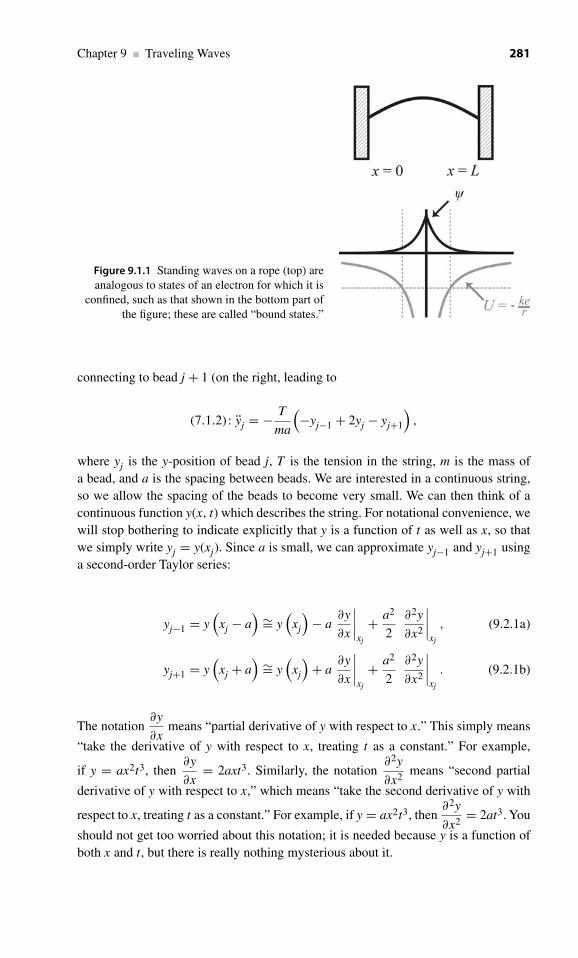
Chapter 9 ■ Traveling Waves 281
Figure 9.1.1 Standing waves on a rope (top) areanalogous to states of an electron for which it is
confined, such as that shown in the bottom part ofthe figure; these are called “bound states.”
connecting to bead j + 1 (on the right, leading to
(7.1.2) : yj = − T
ma
(−yj−1 + 2yj − yj+1
),
where yj is the y-position of bead j, T is the tension in the string, m is the mass ofa bead, and a is the spacing between beads. We are interested in a continuous string,so we allow the spacing of the beads to become very small. We can then think of acontinuous function y(x, t) which describes the string. For notational convenience, wewill stop bothering to indicate explicitly that y is a function of t as well as x, so thatwe simply write yj = y(xj). Since a is small, we can approximate yj−1 and yj+1 usinga second-order Taylor series:
yj−1 = y(
xj − a) ∼= y
(xj
)− a
∂y
∂x
∣∣∣∣xj
+ a2
2
∂2y
∂x2
∣∣∣∣xj
, (9.2.1a)
yj+1 = y(
xj + a) ∼= y
(xj
)+ a
∂y
∂x
∣∣∣∣xj
+ a2
2
∂2y
∂x2
∣∣∣∣xj
. (9.2.1b)
The notation∂y
∂xmeans “partial derivative of y with respect to x.” This simply means
“take the derivative of y with respect to x, treating t as a constant.” For example,
if y = ax2t3, then∂y
∂x= 2axt3. Similarly, the notation
∂2y
∂x2means “second partial
derivative of y with respect to x,” which means “take the second derivative of y with
respect to x, treating t as a constant.” For example, if y = ax2t3, then∂2y
∂x2= 2at3. You
should not get too worried about this notation; it is needed because y is a function ofboth x and t, but there is really nothing mysterious about it.
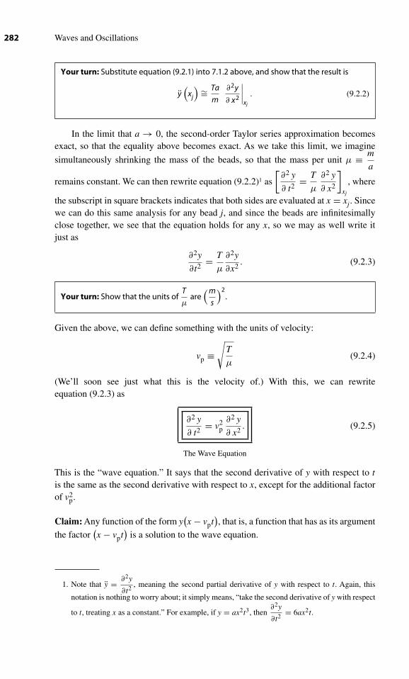
282 Waves and Oscillations
Your turn: Substitute equation (9.2.1) into 7.1.2 above, and show that the result is
y(xj
) ∼= Ta
m
∂2y
∂ x2
∣∣∣∣xj
. (9.2.2)
In the limit that a → 0, the second-order Taylor series approximation becomesexact, so that the equality above becomes exact. As we take this limit, we imagine
simultaneously shrinking the mass of the beads, so that the mass per unit μ ≡ m
a
remains constant. We can then rewrite equation (9.2.2)1 as
[∂2 y
∂ t2= T
μ
∂2 y
∂ x2
]xj
, where
the subscript in square brackets indicates that both sides are evaluated at x = xj. Sincewe can do this same analysis for any bead j, and since the beads are infinitesimallyclose together, we see that the equation holds for any x, so we may as well write itjust as
∂2y
∂t2= T
μ
∂2y
∂x2. (9.2.3)
Your turn: Show that the units ofT
μare
(m
s
)2.
Given the above, we can define something with the units of velocity:
vp ≡√
T
μ(9.2.4)
(We’ll soon see just what this is the velocity of.) With this, we can rewriteequation (9.2.3) as
∂2 y
∂ t2= v2
p∂2 y
∂ x2. (9.2.5)
The Wave Equation
This is the “wave equation.” It says that the second derivative of y with respect to tis the same as the second derivative with respect to x, except for the additional factorof v2
p.
Claim: Any function of the form y(x − vpt
), that is, a function that has as its argument
the factor(x − vpt
)is a solution to the wave equation.
1. Note that y = ∂2y
∂t2, meaning the second partial derivative of y with respect to t. Again, this
notation is nothing to worry about; it simply means, “take the second derivative of y with respect
to t, treating x as a constant.” For example, if y = ax2t3, then∂2y
∂t2= 6ax2t.
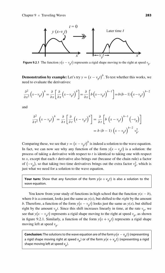
Chapter 9 ■ Traveling Waves 283
Figure 9.2.1 The function y(x − vpt
)represents a rigid shape moving to the right at speed vp.
Demonstration by example: Let’s try y = (x − vpt
)b. To test whether this works, we
need to evaluate the derivatives:
∂2
∂ x2
(x−vpt
)b = ∂
∂ x
[∂
∂ x
(x−vpt
)b]= ∂
∂ x
[b(
x−vpt)b−1
]=b (b−1)
(x−vpt
)b−2
and
∂2
∂ t2
(x − vpt
)b = ∂
∂ t
[∂
∂ t
(x − vpt
)b]
= ∂
∂ t
[b(
x − vpt)b−1 (−vp
)]
= b (b − 1)(
x − vpt)b−2
v2p.
Comparing these, we see that y = (x − vpt
)bis indeed a solution to the wave equation.
In fact, we can now see why any function of the form y(x − vpt
)is a solution: the
process of taking a derivative with respect to t is identical to taking one with respectto x, except that each t derivative also brings out (because of the chain rule) a factorof
(−vp
), so that taking two time derivatives brings out the extra factor v2
p, which isjust what we need for a solution to the wave equation.
Your turn: Show that any function of the form y(x + vpt
)is also a solution to the
wave equation.
You know from your study of functions in high school that the function y(x − b),where b is a constant, looks just the same as y(x), but shifted to the right by the amountb. Therefore, a function of the form y
(x − vpt
)looks just the same as y(x), but shifted
right by the amount vpt. Since this shift increases linearly in time, at the rate vp, we
see that y(x − vpt
)represents a rigid shape moving to the right at speed vp, as shown
in figure 9.2.1. Similarly, a function of the form y(x + vpt
)represents a rigid shape
moving left at speed vp.
Conclusion: The solutions to the wave equation are of the form y(x − vpt
)(representing
a rigid shape moving right at speed vp) or of the form y(x + vpt
)(representing a rigid
shape moving left at speed vp).

284 Waves and Oscillations
So, we see that the string can indeed sustain traveling waves, with speed vp =√T
μ. Note that each infinitesimal segment of the string moves straight up and down
(in the + or −y direction) as the wave passes, even though the wave is moving rightor left (in the + or −x direction).
There is something quite remarkable about the conclusion in the box above: thespeed of the wave, vp, doesn’t depend on the shape. In particular, for sinusoidal wavesthe speed doesn’t depend on the wavelength or the amplitude!
9.3 Traveling sinusoidal waves
The most important example of a traveling wave is a sinusoid; We know from Fourieranalysis that any function can be formed by summing up sinusoids. Recall from
chapter 7 that a sine wave of wavenumber k = 2π
λ(where λ is the wavelength) and
amplitude A is written A sin kx. To make this travel to the right, we simply replace xby
(x − vpt
):
y = A sin[k(
x − vpt)]
= A sin(
kx − kvpt)
. (9.3.1)
When t advances from 0 to2π
k vp, the argument of the sin increases by 2π . Therefore,
the period of the wave is T = 2π
k vp. Since the angular frequency is given by ω ≡ 2π
T,
we see that ω = kvp ⇔
vp = ω
k. (9.3.2)
This is really nothing new. You’ve known since you were a toddler that the speed
of a sinusoidal wave is given by v = λ
T. We can reexpress this in terms of k and ω:
v = λ
T= 2π/k
2π/ω= ω
k.
Using equation (9.3.2), we can rewrite equation (9.3.1), to express a right-travelingsinusoidal wave as
y = A sin (k x − ω t) ,
which is the most common way of writing it. The speed of the wave is the speed atwhich the crest (corresponding to a phase of 90
◦) or the trough (corresponding to a
phase of 270◦) advances, so it is called the “phase velocity,” hence the use of “p” as a
subscript in vp.

Chapter 9 ■ Traveling Waves 285
9.4 The superposition principle for traveling waves
In section 4.4, we found that when an oscillator is driven by multiple drive forces,the resulting response is simply the sum of the responses to each drive force on itsown. This is a consequence of the linearity of the differential equation governing theoscillator. In this section, we explore a related consequence of linearity, but this timefor a system that is not driven. In particular, we will explore whether we can combineleft- and right-moving waves, and what happens when they “collide.”
Claim: For any differential equation that is linear (i.e., there are no terms proportionalto y2 or to y y, etc.) and homogeneous (i.e., there are no terms that are constant), if yAis a solution to the differential equation, and yB is a different solution, then the linearcombination AyA + ByB (where Aand B are constants) is also a solution.
Proof for the wave equation: To say that yA is a solution to the wave equation simplymeans that
∂2 yA
∂ t2= v2
p∂2 yA
∂ x2. (9.4.1)
Similarly, to say that yB is a solution simply means that
∂2 yB
∂ t2= v2
p∂2 yB
∂ x2. (9.4.2)
Now, we multiply equation (9.4.1) by A, multiply equation (9.4.2) by B and add themtogether:
A∂2yA
∂ t2+B
∂2yB
∂ t2=v2
p
(A
∂2yA
∂ x2+B
∂2yB
∂ x2
)⇔ ∂2
(AyA +ByB
)∂ t2
=v2p
∂2
∂ x2
(AyA +ByB
),
which shows that AyA + ByB is a solution to the wave equation. (Perhaps you can seehow you could do this same type of proof for any linear, homogeneous differentialequation.)
This principle of superposing (i.e., adding together) solutions is a very powerfulone, and one that you will use a lot in quantum mechanics, which is governed by theSchrodinger equation
− h2
2 m
∂2�
∂ x2+ U � = ih
∂ �
∂ t, (9.4.3)
where m is the mass of the electron, U is the potential energy of the electron, and� (x, t) is the electron wavefunction, which is analogous to y (x, t). You can see thatthis differential equation is linear (i.e., it contains no terms proportional to �2 or to� �, etc.) and homogeneous (i.e., it contains no constant terms), so it must obey thePrinciple of Superposition.
As applied to waves that obey the wave equation, the Principle means, for example,that we can have left- and right-traveling waves propagating at the same time. As theymove into the same area, they simply add up, as shown in figure 9.4.1, but they don’talter each other in any profound way – each just keeps going, and eventually they passthrough each other with no change!

286 Waves and Oscillations
Figure 9.4.1 For waves governed by a lineardifferential equation, left- and right-travelingwaves simply add together, and pass through eachother without other effect; this is the Principle ofSuperposition.
Recall from chapter 7 that when a string is stretched between two walls, that is,when we impose the boundary conditions that y = 0 at x = 0 and x = L, the solutionsare standing waves. The basic physics of the string that we used in chapter 7 are exactlythe same as the physics we used to derive the wave equation. We know that the left- andright-traveling wave solutions are the only solutions to the wave equation, so it must bepossible to express standing waves as a superposition of traveling waves. For example,a pure normal mode n of a string between two walls is
y = Cn sin knx cos ωnt. (9.4.4)
(Note how, for a standing wave such as this, the time and space dependence appearin the arguments of two different functions, whereas for a traveling wave they appeartogether in the argument of one function.) Can we express this as a superposition oftraveling waves?
Your turn: Use the basic trig identity sin (A + B) = sin A cos B + cos A sin B to show that
Cn
2sin
(knx + ωnt
) + Cn
2sin
(knx − ωnt
) = Cn sin knx cos ωnt,
that is, that the sum of two equal-amplitude waves traveling in opposite directions
produces a standing wave!
This result is important in a number of contexts. For example, in solid-state physicsthe “energy gaps” which are responsible for the electronic properties of semiconductorsarise as the result of a standing wave which forms when electron waves of certainspecial wavelengths undergo diffraction from the lattice of atoms in the semiconductorcrystal, creating a “backscattered” wave which travels in the opposite direction fromthe original, and has the same amplitude.

Chapter 9 ■ Traveling Waves 287
Note that standing waves are a special case, because of the imposition of theboundary conditions. Therefore, although we can superpose the more general solutions(traveling waves) to create the special case solution (standing waves), we can’tgo the other way, that is, we can’t superpose standing waves to create travelingwaves.
9.5 Electromagnetic waves in vacuum
The phenomena of electricity and magnetism are governed by Maxwell’s fourequations:
Gauss’s Law:
∮E · n dA = Qnet, enclosed
ε0(9.5.1)
“Electric field lines can only begin on + charges and can only end on − charges.
The electric field due to a point charge is given by E = 14πε0
Q
r2 ”
Gauss’s Law for magnetic fields:
∮B · n dA = 0 (9.5.2)
“There are no magnetic monopoles.”
Faraday’s Law:
∮E · d
⇀
� = − ddt
∫B · n dA (9.5.3)
“A time-varying B creates a spatially varying E.”
Ampère’s Law:
∮B · d
⇀
� = μ0 Inetthreading
+μ0ε0ddt
∫E · n dA (9.5.4)
“Magnetic fields are created by currents or by time-varying E.”
Maxwell’s equations restrict which combinations of electric fields, magnetic fields,and charge are allowed. For example, the magnetic field pattern shown in figure 9.5.1is not allowed by equation (9.5.2). Let us ask whether “plane waves” are allowed in
Figure 9.5.1 This magnetic field is not consistent withequation (9.5.2).
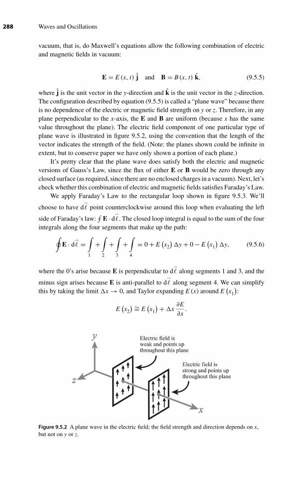
288 Waves and Oscillations
vacuum, that is, do Maxwell’s equations allow the following combination of electricand magnetic fields in vacuum:
E = E (x, t) j and B = B (x, t) k, (9.5.5)
where j is the unit vector in the y-direction and k is the unit vector in the z-direction.The configuration described by equation (9.5.5) is called a “plane wave” because thereis no dependence of the electric or magnetic field strength on y or z. Therefore, in anyplane perpendicular to the x-axis, the E and B are uniform (because x has the samevalue throughout the plane). The electric field component of one particular type ofplane wave is illustrated in figure 9.5.2, using the convention that the length of thevector indicates the strength of the field. (Note: the planes shown could be infinite inextent, but to conserve paper we have only shown a portion of each plane.)
It’s pretty clear that the plane wave does satisfy both the electric and magneticversions of Gauss’s Law, since the flux of either E or B would be zero through anyclosed surface (as required, since there are no enclosed charges in a vacuum). Next, let’scheck whether this combination of electric and magnetic fields satisfies Faraday’s Law.
We apply Faraday’s Law to the rectangular loop shown in figure 9.5.3. We’ll
choose to have d⇀
� point counterclockwise around this loop when evaluating the left
side of Faraday’s law:∮
E · d⇀
� . The closed loop integral is equal to the sum of the fourintegrals along the four segments that make up the path:∮
E · d⇀
� =∫1
+∫2
+∫3
+∫4
= 0 + E(x2
)y + 0 − E
(x1
)y, (9.5.6)
where the 0’s arise because E is perpendicular to d⇀
� along segments 1 and 3, and the
minus sign arises because E is anti-parallel to d⇀
� along segment 4. We can simplifythis by taking the limit x → 0, and Taylor expanding E (x) around E
(x1
):
E(x2
) ∼= E(x1
) + x∂E
∂x.
Figure 9.5.2 A plane wave in the electric field; the field strength and direction depends on x,but not on y or z.

Chapter 9 ■ Traveling Waves 289
Figure 9.5.3 Geometry forapplying Faraday’s Law to the
plane wave (9.5.5).
Plugging this into equation (9.5.6) gives∮E · d
⇀
� ∼= ∂E
∂xx y. (9.5.7)
The equality becomes exact in the limit x → 0.
Now we turn our attention to the right side of Faraday’s Law: − d
dt
∫B · n dA. The
direction of n is determined by our choice of the directionality of d⇀
�: curl the fingers
of your right hand in the direction of d⇀
� , and your thumb points in the direction ofn, along k in this case. The form of the magnetic field we’re investigating is (9.5.5):B = B (x, t) k, therefore B · n = B (x, t). Since x is infinitesimal, and since B doesn’tdepend on y, B is uniform over the area bounded by the loop. Therefore, B · n =B x y. Plugging this and equation (9.5.7) into Faraday’s Law (9.5.3) gives
∂E
∂xx y = −∂B
∂tx y ⇒
∂E
∂x= −∂B
∂t. (9.5.8)
So, fields of the form E = E (x, t) y and B = B (x, t) z are allowed by Faraday’s law,so long as E and B are related as shown by equation (9.5.8).
There is one more Maxwell equation that we must check, Ampère’s law:∮B · d
⇀
� = μ0 Inetthreading
+μ0ε0d
dt
∫E · n dA.
Since we are considering fields in a vacuum, Inetthreading
= 0. The reasoning following
from this is almost exactly the same as the reasoning for Faraday’s law. You can showin problem 9.6 that the result is
∂B
∂x= −μ0ε0
∂E
∂t. (9.5.9)

290 Waves and Oscillations
Let’s combine equations (9.5.9) with (9.5.8). We begin by taking∂
∂xof both sides of
equation (9.5.8), giving
∂2E
∂2x= − ∂
∂x
∂B
∂t= − ∂
∂t
∂B
∂x.
Now, we use equation (9.5.9) to substitute for∂B
∂x, giving
∂2E
∂2x= − ∂
∂t
(−μ0ε0
∂E
∂t
)⇒
∂2E
∂2x= μ0ε0
∂2E
∂t2.
This is the wave equation, (9.2.5):∂2 y
∂ t2= v2
p∂2 y
∂ x2, with E playing the role of y, and
phase velocity
c = 1√ε0μ0
(9.5.10)
If you plug in the numbers on this, you find a speed of 2.998 × 10⁸ m/s, exactly equalto the speed of light!
What about the magnetic field? You can make any wave by adding up sinusoids.So, for simplicity, let’s consider
E = E0 sin k (x − ct) j.
Since the phase velocity c = ω/k, we can rewrite this as E = E j with
E = E0 sin (kx − ωt) . (9.5.11)
Plugging this into equation (9.5.8):∂E
∂x= −∂B
∂tgives
∂B
∂t= −E0k cos(kx − ωt)
integrate withrespect to t−−−−−−−→ B = E0
k
ωsin (kx − ωt) + const.
Because we are interested in waves, we’ll set the constant equal to zero. (The presenceof the constant means that we’re allowed to have a uniform, constant magnetic fieldin addition to the electromagnetic wave.) Since c = ω/k, this gives
B = E01
csin (kx − ωt) = E
c⇒
E = cB. (9.5.12)
Relation between amplitudes of E and B for an electromagnetic wave in vacuum
Because of this direct proportionality, we see that the electric and magnetic componentsof the wave are in phase. This means that the magnetic field also propagates as a wave,moving at speed c.

Chapter 9 ■ Traveling Waves 291
We have just shown that plane waves are allowed by all four of Maxwell’sequations, but only if they travel at speed c and have E = cB. These electromagneticwaves (which include light, radio waves, X-rays, microwaves, gamma rays, etc.)consist of a self-sustaining oscillation, in which the changing magnetic field createsa changing electric field, which in turn creates a changing magnetic field, etc. Thewhole thing can only keep going if it travels at exactly c. The realization that thespeed of light is a consequence of Maxwell’s equations led directly to Einstein’stheory of special relativity: If we assume that the laws of physics are the same inall reference frames traveling at constant velocity, then Maxwell’s equations mustapply equally well in all such frames, and the speed of light must be exactly the samein all such frames. This is the basic postulate of special relativity, and immediatelyleads to such counterintuitive results as the speed of a light beam emanating from theflash light being exactly the same as perceived in the frame in which the flashlightis at rest as it is in a frame moving at speed 0.999 c in the direction the beam istraveling!
Your turn: On the previous page, we showed that E (x, t) = cB (x, t) for a wave movingin the positive x-direction, meaning that the E and B waves are in phase. Now, show thatE (x, t) = −cB (x, t) for a wave moving along the negative x-direction, meaning that theE and B waves are out of phase.
For any electromagnetic (em) wave, the propagation direction is given by the“Poynting vector”:
S = 1
μ0E × B. (9.5.13)
(The fortuitously named John Henry Poynting was a student of Maxwell.) Insection 9.10, we’ll see that this vector not only points in the direction of prop-agation, but also has a magnitude equal to the intensity (power per area) ofthe wave.
At the risk of being repetitive, let us reinforce the true nature of a plane wave,the type of wave we’ve been discussing. Recall that we began with the assumption(9.5.5) that E and B depend on x, but not on y or z. Some students misinterpretthis to mean that the wave exists only as a ray along the x-axis. This incorrectthinking is reinforced by the usual graphical way of portraying a plane wave, shownin figure 9.5.4a. This shows the magnitudes of E and B for points along the x-axis,using the convention that the length of the vector represents the strength of the field.However, this picture must not be taken to mean that E and B are zero at pointsthat aren’t on the x-axis. Instead, since E and B depend only on x, and not on yor z, the picture would be the same for any line parallel to the x-axis, as shownin figure 9.5.4b. Figure 9.5.5 shows the correspondence between the two ways ofportraying the strength of the electric field. In the foreground, the strength is indicatedby the spacing between field lines; this emphasizes that the field extends throughoutspace, and is has the same strength and direction throughout any plane perpendicularto the x-axis. In the background, the strength of the field is indicated by the length of thevectors.

Figure 9.5.4 a: The conventional way ofportraying an electromagnetic wave,showing the magnitudes of the electric andmagnetic fields along the x-axis. b: Anotherportrayal, emphasizing that the magnitudesof the fields are equal at equivalent pointsalong any line parallel to the x-axis.
Figure 9.5.5 Two ways of portraying a plane wave of the electric field.
292

Chapter 9 ■ Traveling Waves 293
Key equations for isomorphisms. Over the rest of this chapter, we will developisomorphisms (exact analogies) between em waves in vacuum and various other typesof waves. The essential relations are:
(9.5.8) : ∂E
∂x= −∂B
∂tand (9.5.9) : ∂B
∂x= −μ0 ε0
∂E
∂t.
All the other results follow from these two relations, including the fact that the twocomponents of the wave (in this case E and B) each obey the wave equation, therelation between the magnitude of the two components (E = cB), and the speed of
the wave c = 1√ε0μ0
. So, if we can find equations relating the two components of
a wave that are isomorphic to equations (9.5.8) and (9.5.9), then there is a complete
isomorphism. It will sometimes make things a bit easier to substitute c = 1√ε0μ0
into
equation (9.5.9), so that the two essential relations become
(9.5.8) : ∂E
∂x= −∂B
∂t
and∂B
∂x= − 1
c2
∂E
∂t. (9.5.14)
Isomorphism with rope waves. As a guide to developing the isomorphism betweenrope waves and em waves in vacuum, we refer back to the isomorphism between themechanical oscillator and the electrical oscillator. From section 1.5, we have:
Table 9.5.1. Isomorphism between mechanical and electrical oscillators
Mass and spring Electrical oscillator
Position relative to equilibrium x Charge q on capacitorMass m Inductance LSpring constant k Inverse capacitance 1/C
For the mechanical oscillator, the oscillations are a result of the restoring forcewhich tends to bring the system back toward equilibrium and the momentum whichtends to make the system overshoot the equilibrium point. The restoring force isassociated with the spring constant k which is isomorphic to 1/C. The capacitor isassociated with electric fields. Therefore, we may expect some type of connectionbetween the restoring force in a rope and the E for the em wave. The momentumis associated with the mass m which is isomorphic to L. The inductor is associatedwith magnetic fields. Therefore, we may expect some type of connection between themomentum of a rope wave and the B for the em wave.
Now, let’s get more quantitative. For a rope wave, we speak of the mass per length,μ, rather than simply the mass (which would be infinite for an infinitely long rope).
Thus, the transverse momentum per unit length is given by μ∂y
∂t. For simplicity, we
will refer to this as the “momentum wave,” and use the symbol py ≡ μ∂y
∂t, bearing in
mind that this is really the transverse momentum per unit length. We will hope thatthis is isomorphic to B, and search for the quantity (related to the restoring force) thatis isomorphic to E.
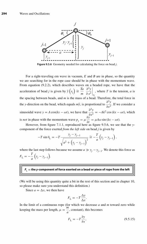
294 Waves and Oscillations
Figure 9.5.6 Geometry needed for calculating the force on bead j.
For a right-traveling em wave in vacuum, E and B are in phase, so the quantitywe are searching for in the rope case should be in phase with the momentum wave.From equation (9.2.2), which describes waves on a beaded rope, we have that the
acceleration of bead j is given by y(
xj
) ∼= Ta
m
∂2y
∂ x2
∣∣∣∣xj
, where T is the tension, a is
the spacing between beads, and m is the mass of a bead. Therefore, the total force in
the y-direction on the bead, which equals my, is proportional to∂2y
∂x2. If we consider a
sinusoidal wave y = A cos(kx − ωt), we have that∂2y
∂x2= −Ak2 cos (kx − ωt), which
is not in phase with the momentum wave py = μ∂y
∂t= μAω sin (kx − ωt).
However, from figure 7.1.1, reproduced here as figure 9.5.6, we see that the y-component of the force exerted from the left side on bead j is given by
−T sin θL = −Tyj − yj−1√
a2 +(
yj − yj−1
)2∼= −T
a
(yj − yj−1
),
where the last step follows because we assume a � yj − yj−1. We denote this force as
FL = −T
a
(yj − yj−1
).
FL ≡ the y-component of force exerted on a bead or piece of rope from the left
(We will be using this quantity quite a bit in the rest of this section and in chapter 10,so please make sure you understand this definition.)
Since a = x, we then have
FL = −Ty
x.
In the limit of a continuous rope (for which we decrease a and m toward zero while
keeping the mass per length, μ = m
a, constant), this becomes
FL = −T∂y
∂x, (9.5.15)

Chapter 9 ■ Traveling Waves 295
where now we interpret this as the y-component of the force exerted from the left sideon a tiny segment of the rope. To check whether this is in phase with the momentumwave, we again consider the sinusoidal wave y = A cos(kx − ωt). For this, FL =−T
∂y
∂x= TAk sin (kx − ωt), which is in phase with the momentum wave py = μ
∂y
∂t=
μAω sin (kx − ωt).It may seem odd that the y-component of the force exerted from the left should be
so important. However, if you hold the left end of a long rope with your hand, you mustexert a y-component of force (from the left) on this end to start a wave propagatingdown the rope. Saying the same thing in a different way: for right-traveling waves, it isthe y-component of force exerted from the left which is responsible for the propagationof a wavefront to the right on a rope that is initially at equilibrium; the force from theleft is what pulls an initially quiescent piece of rope away from equilibrium. We willsee in chapter 10 that this idea of the y-component of force exerted from the left is quiteimportant for the behavior of right-traveling waves when they encounter an interfacebetween two ropes with different values of μ.
So, are the momentum wave py ≡ μ∂y
∂tand the y-force-from-the-left wave
FL = −T∂y
∂xrelated in the same ways as B and E? From equation (9.2.2), we have for
the beaded rope
∂2y(
xj
)∂t2
= Ta
m
∂2y
∂ x2
∣∣∣∣xj
⇔T∂2y
∂ x2
∣∣∣∣xj
= m
a
∂2y(
xj
)∂t2
⇒− ∂
∂x
[−T
∂y
∂x
]= ∂
∂t
[m
a
∂y
∂t
]⇒
∂
∂xFL =− ∂
∂t
[μ
∂y
∂t
]isomorphicwith←−−−−−−−−→(9.5.8): ∂E
∂x=−∂B
∂t.
We see that, in the isomorphism for this equation, FL plays the role of E, and py ≡ μ∂y
∂tplays the role of B, as expected.
To complete the isomorphism between rope waves and em waves in a vacuum,we need to find the equation for a rope that is isomorphic with equation (9.5.14):∂B
∂x= − 1
c2
∂E
∂t. Because the order of derivatives doesn’t matter, we have
∂
∂x
∂y
∂t= ∂
∂t
∂y
∂x.
From equation (9.2.4), vp ≡√
T
μ⇒ μ = T
v2p
. Combining this with the above gives
μ∂
∂x
∂y
∂t= T
v2p
∂
∂t
∂y
∂x⇒ ∂
∂x
[μ
∂y
∂t
]= − 1
v2p
∂
∂t
[−T
∂y
∂x
]⇒
∂
∂xpy = − 1
v2p
∂
∂tFL
isomorphic with←−−−−−−−−→(9.5.14) : ∂B
∂x= − 1
c2
∂E
∂t.
So, there is a complete isomorphism between rope waves and em waves in a vacuum.
Therefore, there is a isomorphism between the phase velocity for rope waves, vp =√
T
μ,

296 Waves and Oscillations
Table 9.5.2. Isomorphism between rope waves and electromagnetic waves in a vacuum
Rope waves Electromagnetic waves in vacuum
Transverse velocity y B/μ0y-component of force from the left Electric field E
FL = −T∂y
∂xMass per length μ Permeability of free space μ0Tension T Inverse of permittivity of free space: 1/ε0
and the phase velocity for em waves in a vacuum, c = 1√μ0 ε0
. However, it is not clear
whether we can push things further than this. For example, is T isomorphic to 1/μ0 andμ isomorphic to ε0, or instead is T isomorphic to 1/ε0 and μ isomorphic to μ0? Sinceμ is associated with momentum (which is isomorphic to B) and μ0 is associated withB, one might expect that μ might be isomorphic to μ0. Further, since T is associatedwith the force from the left (which is isomorphic to E ) and ε0 is associated with E,one might expect that T is isomorphic to 1/ε0. In problem 9.5, you can show that these
are indeed the correct isomorphisms. Since py ≡ μ∂y
∂tis isomorphic to B and μ is
isomorphic to μ0, we see that y = ∂y
∂tis isomorphic to B
/μ0, and this version of the
isomorphism turns out to be somewhat more useful.The remaining isomorphisms with other types of waves will take a lot less effort
to develop!
Self-test: Use this isomorphism and E = cB first to show that the FL wave is in phase
with the y wave, and then to show that∂y
∂t= −vp
∂y
∂xfor a rope wave. (You should find
this helpful for problem 9.2. You can derive this expression using a different methodin problem 9.1.)
Since E = cB for right-moving em waves in vacuum, the E and B waves are inphase. By the isomorphism, this means that the FL and y waves are in phase for right-moving rope waves. For left-moving waves, E = −cB (as you showed earlier in thissection), so E and B are out of phase. By the isomorphism, this means that the FL andy waves are out of phase for left-moving rope waves.
9.6 Electromagnetic waves in matter
A full description of electric and magnetic fields in matter is well beyond this text.For a deeper understanding, you should consult an introductory electrodynamics text.2
2. The best treatment at the undergraduate level is Introduction to Electrodynamics, 3rd Ed.,by David J. Griffiths (Prentice-Hall, Upper Saddle River, NJ, 1999).

Chapter 9 ■ Traveling Waves 297
Figure 9.6.1 Part a: when electric dipoles alignwith a field, the field they create opposes the
applied field. Part b: when magnetic dipoles alignwith a field, the field they create enhances the
applied field.
What follows is just the basics for simple geometries and the most commonmaterials.
When the space between the plates of a parallel plate capacitor is filled with aninsulating material, the atoms and molecules within the material become polarizedby the electric field; each atom or molecule becomes an electric dipole, as shownschematically in figure 9.6.1a. (Note that the polarization is caused not only by thefield due to the plates, but instead by the combined field of the plates and all the otherdipoles in the material.) If we consider a line of such dipoles within the material, wesee that the electric field due to the dipoles opposes the electric field due to the plates,so that the total field between the plates is reduced. The factor of reduction is calledthe dielectric constant:
κ = Eplates
Etotal. (9.6.1)
The parallel plate capacitor provides a particularly simple geometry; in a morecomplicated geometry, the relationship between the total field and the field due tothe “free charge” (the charge on the plates) is more complicated. For almost allmaterials, the dielectric constant really is constant, meaning that it doesn’t dependon the strength of the electric field (at least until the field gets quite strong). Anotherway of saying this is that the degree of polarization is linearly proportional to thetotal electric field. We will focus exclusively on these “linear materials,” thoughyou should be aware that there are some materials for which the behavior is morecomplicated.
An insulating material is also called a “dielectric,” derived from the Greek “dia”meaning “through,” therefore indicating that an electric field can penetrate through adielectric. This is a bit of a misnomer, since the dielectric constant for typical insulatingsolids is from about 2–8, meaning that the field in a parallel plate capacitor is reducedby a factor of 2–8 by the presence of the dielectric. We define the permittivity of thedielectric material to be
ε = κε0. (9.6.2)
Thus, ε is always greater than or equal to ε0.

298 Waves and Oscillations
Similarly, when the space inside a solenoid is filled with matter, the magneticdipoles associated with the spin of the electrons and with the orbital motion ofthe electrons are affected by the magnetic field. The effect on the electron spinsis shown schematically in figure 9.6.1b. Again, the dipoles associated with theelectron spin align “with” the field of the solenoid coil (meaning that the north poleof each dipole is on the right, and the south pole on the left), but for magneticdipoles the field due to the dipole within the dipole points from south to north,in the same direction as the field from the coil. (This is opposite to what happensfor an electric dipole; inside the dipole, the field due to the dipole points frompositive to negative.) Therefore, the field of the spin dipoles enhances the field dueto the coils somewhat. A material with this type of behavior is therefore called“paramagnetic,” from the Greek “para” meaning “alongside.” However, in othermaterials, the magnetic response is dominated by the interaction with the orbital motionof the electron, which is more complicated. The net effect of this interaction is to makethe magnetic moment associated with the orbital motion align opposite the field ofthe coils. Thus, if the solenoid is filled with a material dominated by this type ofresponse, the total field is smaller than without the material. Such materials are called“diamagnetic.” Again, we restrict ourselves to linear materials for which the degreeof polarization is proportional to the total field. We define the permeability of thematerial to be
μ = μ0
(1 + χm
), (9.6.3)
where χm (Greek letter “chi”-sub-m) is the “magnetic susceptibility.” For diamagneticmaterials, the susceptibility is negative, and typically ranges from 10−6 to 10−5. Forparamagnetic materials, the susceptibility is positive, and typically ranges from 10−5
to 10−4. In any case, the effect on the total field is quite small, in strong contrast to thecase for dielectrics. (Note that we are not discussing ferromagnetic materials such asiron, which dramatically affect the magnetic field.) Thus, for linear materials, μ is closeto μ0; it is slightly less for diamagnetic materials, and slightly more for paramagneticmaterials.
It is convenient to define a new field called “H”:
H = 1
μB. (9.6.4)
Even for linear materials there is no simple physical interpretation for H other thanwhat is evident from the above equation. Within the material, it is still the magnetic fieldB that exerts the force F = qv × B on moving charges. However, H is calculationallyconvenient. (It turns out that, for symmetrical geometries, you can calculate H justfrom the currents in coils, without referring to the complexities of the diamagnetic orparamagnetic materials.)
The standard form of Maxwell’s equations is still correct within any material,whether linear or not. However, it is sometimes convenient to separate the effects of the“free charges” (such as the charges on capacitor plates and the charges flowing througha solenoid coil) from those of “bound charges” (the charges which rearrange slightlywhen atoms and molecules are polarized by an electric field) and “bound currents” (thecurrents associated with electron spin and orbital motion). To create the alternate set of
Chapter 9 ■ Traveling Waves 299
Maxwell’s equations which is valid in a linear material, we simply replace ε0 by ε, μ0by μ, and all charges by just the free charges. The two equations we care about mostare Faraday’s law and Ampère’s Law. Applying the recipe to Ampère’s Law, we get∮
B · d⇀
� = μ0 Inetthreading
+ μ0 ε0d
dt
∫E · n dA
︸ ︷︷ ︸Ampere’s Law for any circumstance
→
∮B · d
⇀
� = μ Ifreenetthreading
+μ εd
dt
∫E · n dA.
︸ ︷︷ ︸An alternate version of Ampere’s Lawfor an isotropic linear material
We can rearrange this a bit to obtain∮1
μB · d
⇀
� = Ifreenetthreading
+ εd
dt
∫E · n dA.
If we restrict ourselves to materials that are not electrically conducting (so that
Ifreenetthreading
= 0), and make use of H = 1
μB, we get
∮H · d
⇀
� = εd
dt
∫E · n dA . (9.6.5)
Recall that the original version of Ampère’s Law in vacuum,∮
B · d⇀
� = μ0 ε0d
dt∫E · n dA , when applied to a plane wave led to equation (9.5.9),
∂B
∂x= −μ0 ε0
∂E
∂t.
So, we can see that equation (9.6.5) leads to
∂H
∂x= −ε
∂E
∂t⇒
∂ (μH)
∂x= −εμ
∂E
∂t
isomorphic with←−−−−−−−−→(9.5.14) : ∂B
∂x= − 1
c2
∂E
∂t.
We see that μH plays the role of B, E plays the role of E, and εμ plays the role of 1/c2.To complete the isomorphism, we must find the equation for em fields in matter
that is isomorphic to equation (9.5.8):∂E
∂x= −∂B
∂t. If we apply the recipe of replacing
ε0 by ε, μ0 by μ, and all charges by just the free charges to Faraday’s Law, there is nochange:∮
E · d⇀
� = − d
dt
∫B · n dA︸ ︷︷ ︸
Faraday’s Law for any circumstance
−→∮
E · d⇀
� = − d
dt
∫B · n dA.︸ ︷︷ ︸
An alternate version of Faraday’s Lawfor linear materials

300 Waves and Oscillations
However, since B = μ H, we can rewrite this as
∮E · d
⇀
� = − d
dt
∫μ H · n dA. (9.6.6)
Recall that the original version of Faraday’s law when applied to a plane wave led to
equation (9.5.8),∂E
∂x= −∂B
∂t, so we can see that equation (9.6.6) leads to
∂E
∂x= −∂ (μH)
∂t
isomorphic with←−−−−−−−−→(9.5.8) : ∂E
∂x= −∂B
∂t.
Thus, the isomorphism between em waves in a vacuum and em waves in linearmaterials is complete. As for the case with rope waves, it will be convenient to writethe isomorphism in terms of B/μ0, which is isomorphic to μH/μ = H:
Table 9.6.1. Isomorphism between electromagnetic waves in linear materials and in a vacuum
Electromagnetic waves in linear materials Electromagnetic waves in vacuum
H B/μ0Electric Field E Electric Field EPermeability μ Permeability of free space μ0Permittivity ε Permittivity of free space ε0
Since B = μH, you may well ask, “Why bother to write H in the isomorphismrather than just B/μ”? Indeed, we could well have done so. We will see that when weconsider reflections at a boundary between two different media (with different valuesof μ), it is somewhat easier to phrase things in terms of H.
Concept test (answer below3): What is the speed of em waves in linear materials?
Concept test (answer below4): Recall that in section 9.5 I stated that the intensity
(power per area) for em waves in vacuum is S = 1μ0
E × B. Use this to explain why the
intensity of em waves in linear materials is given by the magnitude of
S = E × H. (9.6.7)
3. In vacuum, c = 1√μ0 ε0
, so in linear media vp = 1√μ ε
.
4. From equation (9.5.13), in vacuum S = 1
μ0E × B = E ×
(Bμ0
). Using the isomorphism,
this translates into S = E × H.

Chapter 9 ■ Traveling Waves 301
Concept test (answer below5): Explain why the intensity of em waves in linear materialsis given by
S =√
ε
μE2. (9.6.8)
9.7 Waves on transmission lines
One of the two most important applications for em waves is the transmission ofinformation. For example, we use em waves for radio and television broadcasts.However, we frequently want to have better control of where information goes, and forthese applications we use cables, such as those used for telephone, cable TV, computernetworks, speaker wires, and so on. Such cables are called “transmission lines” byphysicists. The information is always transmitted through a pair of conductors. For atelephone line, there are two wires twisted together. For cable TV, there is a centralwire surrounded by a cylindrical outer conductor, with plastic insulation between.(This is called a “coaxial cable.”) For transmission of information on circuit boards,the transmission line often consists of a wire above a sheet of metal called a “groundplane”; the ground plane acts as the second conductor. Sometimes, the metal chassisof an apparatus, or the ground itself, is used as one of the two conductors needed fora transmission line.
Depending on the system, the information is either represented by the time-varyingvoltage difference between the two conductors, or by the time-varying current travelingthrough them (into a target device on one wire, and back out on the other). No matterwhether the information is transmitted by applying a controlled voltage to one end ofthe transmission line or by applying a controlled current, it propagates as a linked waveof current and voltage travelling along the line. The current creates a magnetic field,and the voltage difference between the two conductors is associated with an electricfield between them, so that the wave is actually a self-sustaining em phenomenon;the mathematics are analogous to those for an em wave in a vacuum, with the currentanalogous to B and the voltage analogous to E. We will see that, in a standard coaxialcable such as you may have used in the laboratory to connect electrical signals to anoscilloscope, the wave travels at 2/3 c.
Our reasoning about these waves begins with two points: (i) Any two conductorsthat aren’t infinitely far apart have a capacitance between them. (ii) Any length of wire,even if it’s straight, has some inductance. One way to see this is that when you run acurrent through a straight wire, it sets up a magnetic field. It takes energy to create this
5. From (9.5.12), E = cB = 1√μ0 ε0
μ0
(B
μ0
)=
√μ0
ε0
(B
μ0
). This translates into E =
√μ
εH ⇔
H =√
ε
μE. Substituting this into equation (9.6.7) gives equation (9.6.8).

302 Waves and Oscillations
Figure 9.7.1 Model for a transmission line.
field (recall from introductory electricity and magnetism that there is an energy densityassociated with the magnetic field), so you know by a Lenz’s law type of argumentthat this means it will be “harder” to start current flowing through the wire, which is
exactly the characteristic of an inductor: V = LdI
dtis the voltage produced across an
inductor when the current through it is changed, in the same way that V = IR is thevoltage produced across a resistor when the current I flows through it.
Using (i) and (ii), you should now find it reasonable that any transmission linecan be modeled as a series of inductors along one wire (the top wire in figure 9.7.1)and capacitors to the other wire, as shown. For a coaxial cable, the top wire would bethe inner conductor and the lower wire would be the cylindrical outer conductor. Forthe single wire running above a ground plane, the top wire would be the wire runningabove the ground and the lower wire would be the ground plane. We begin with the“lumped circuit element” model shown; very soon, we will take the limit where thesize of each cell in the model becomes infinitesimally small, corresponding to the limitof a continuous transmission line. For mathematical simplicity, we assume the lowerwire is grounded, that is, that it is at zero voltage. We define the current circulatingwithin each cell to be positive when it is moving clockwise, as shown, that is, movingto the right on the top wire and to the left on the bottom wire.
We will find an isomorphism between this system and em waves in vacuum.
Your turn: (a) Explain briefly why Ij−1 − Ij = dqj
dt, and why this equals C
dVj
dt.
(b) Explain briefly why LdIjdt
= Vj − Vj+1
From the result of part (b), we have
LdIj
dt= Vj − Vj+1 = −
(Vj+1 − Vj
)≡ −V .
Dividing both sides of this by the cell size a gives
L
a
dIj
dt= −V
a⇔ V
a= −L
a
dIj
dt.

Chapter 9 ■ Traveling Waves 303
We define L0 to be the inductance per unit length. Therefore L/alim a→0−−−−−→ L0 . So, in
the limit that the cell size becomes infinitesimal, the above becomes
∂V
∂x= −L0
∂I
∂t⇔
∂V
∂x= −∂
(L0I
)∂t
isomorphic with←−−−−−−−−→(9.5.8) : ∂E
∂x= −∂B
∂t.
In the isomorphism, V plays the role of E, and L0I plays the role of B.To show that the isomorphism is complete, we must find the equation that is
isomorphic to equation (9.5.9):∂B
∂x= −μ0ε0
∂E
∂t. From part (a) of “Your turn” given
earlier, we have
CdVj
dt= Ij−1 − Ij = −
(Ij − Ij−1
)≡ −I.
Dividing both sides of this by the cell size a gives
I
a= −C
a
dVj
dt.
We define C0 to be the capacitance per unit length. Therefore C/alim a→0−−−−−→ C0 . So,
in the limit that the cell size becomes infinitesimal, the above becomes
∂I
∂x= −C0
∂V
∂t⇔
∂(L0I
)∂x
= −L0C0∂V
∂t
isomorphic with←−−−−−−−−→(9.5.9) : ∂B
∂x= −μ0ε0
∂E
∂t.
Again, V plays the role of E and L0I plays the role of B. We also see that the combinationL0C0 plays the role of the combination μ0ε0. As for the isomorphism between ropewaves and em waves in vacuum, it is not clear whether L0 is isomorphic with μ0 and C0with ε0, or instead whether L0 is isomorphic with ε0 and C0 with μ0. However, sinceL0 is associated with the current (which is isomorphic to B), and μ0 is associated withB, one might expect that L0 might be isomorphic to μ0. Further, since C0 is associatedwith the voltage (which is isomorphic to E), and ε0 is associated with E, one mightexpect that C0 is isomorphic to ε0. By considering the power transmitted in the wave,you can show that this hunch is correct; see problem 9.14.
So, the isomorphism between waves on transmission lines and em waves invacuum is complete. For convenience in comparing with other isomorphisms, wesay that 1/C0 is isomorphic to 1/ε0, instead of saying that C0 is isomorphic to ε0(which is equivalent). Also, we write the isomorphism in terms of L0I/L0 = I , whichis isomorphic to B/μ0. See table 9.7.1.
We can use this isomorphism to quickly obtain some important results for waveson transmission lines:
1. Em waves in vacuum are a self-sustaining combination of a wave in E anda wave in B. By the isomorphism, waves on a transmission line are a self-sustaining combination of a wave in Vand a wave in I .

304 Waves and Oscillations
Table 9.7.1. Isomorphism between waves on a transmission line and electromagneticwaves in a vacuum
Waves on a transmission line Electromagnetic waves in vacuum
I B/μ0
V Electric Field E
Inductance per length L0 Permeability of free space μ0
Inverse of capacitance per length: 1/C0 Inverse of permittivity of free space: 1/ε0
2. The speed of em waves in vacuum is c = 1√μ0ε0
, so the phase velocity of
waves on transmission lines is
vp = 1√L0C0
. (9.7.1)
Standard RG58 coaxial cable (the type used in laboratories, and the type that hasa BNC coaxial connector at the end) has C0 = 100 pF/m and L0 = 250 nH/m;
plugging in these numbers gives vp = 1√L0C0
= 2.00 × 10⁸ m/s, or almost
exactly 2/3 c. The coaxial cable typically used for cable television, RG6,has C0 = 53.1pF/m and L0 = 348 nH/m; plugging in these numbers gives
vp = 1√L0C0
= 2.33 × 10⁸ m/s, which is a bit more than 3/4 c.
3. For em waves in vacuum travelling in the positive x-direction, E (x, t) =c B (x, t) = 1√
μ0ε0B (x, t) =
√μ0
ε0
B (x, t)
μ0. Using the isomorphism, this means
that for waves on transmission lines,
V (x, t) =√
L0
C0I (x, t) . (9.7.2)
(Wave traveling in + x-direction)
This means that the current flowing to the right on the top wire is in phasewith the voltage; the current on the bottom wire is always opposite that on thetop wire.
As for em waves in vacuum, for a transmission line wave traveling in the−x-direction, there is a negative sign added to the relation between V and I ,so that
V (x, t) = −√
L0
C0I (x, t) . (9.7.3)
(Wave traveling in − x-direction)

Chapter 9 ■ Traveling Waves 305
9.8 Sound waves
For most of us, sound is second only to light as the most important type of wave.Sounds fill our lives, inform us about our surroundings, and are the main medium forinter-personal relations. Sound is a traveling wave of fluctuations in the pressure anddensity of the air. (All the arguments we will make will work just as well for soundwaves in water or any other medium.) As shown in figure 9.8.1, the fluctuations inpressure P and density ρ are small compared to the background pressure and density.In fact, the fluctuations shown in the picture are greatly exaggerated; in a typical soundwave, the pressure and density only change by about 0.1% of the background value.We define P′ to be the change in pressure relative to the background, and ρ′ to be thechange in density relative to the background, so that
P (t) = P0 + P′ (t) (9.8.1)
and ρ (t) = ρ0 + ρ′ (t) . (9.8.2)
Figure 9.8.1 A sound waveconsists of small variations in
the pressure and density,which are in phase, as shown
in parts (a) and (b). Parts(c)–(e) shown the relationships
between the variation inpressure ρ′, the displacement
δ, and velocity v = dδ/dt. Thedisplacement (δ) and variationin pressure (ρ′) waves are 90
◦
out of phase, but the velocitywave is in phase with the
density wave. The uniformlyspaced dots underneath parts b
and d represent the originalpositions of packets of air
molecules. The arrowsrepresent the displacement
imparted to these packets bythe sound wave, with positivedisplacement δ correspondingto right-pointing arrows. The
bottom row of dots shows thedisplaced positions of the airpackets. From this part of the
figure, you can see how thedisplacement wave gives rise
to the variation in density.

306 Waves and Oscillations
Higher density means higher pressure, so the pressure and density waves are inphase, as shown. As we did for em waves, we will focus on plane waves in our studyof sound, that is, waves in which the pressure and density only depend on x, not on yor z. This means that all points in a plane perpendicular to the x-axis have the samepressure and density.
The density fluctuations are caused by displacements of the air molecules fromtheir evenly spaced positions, as suggested by the dots in the figure which are closertogether at the peaks in the density and by the arrows below the dots which indicate thedisplacements required to achieve this clumping. The displacements point toward thepeaks in the density and away from the valleys. As we did in our study of longitudinalstanding waves, we define the displacement of an air molecule (in the x-direction)relative to its original position to be δ (x, t).
We will show below that the pressure variations are governed by the waveequation, so that we get traveling waves. This means, for example, that we canhave a sinusoidal traveling wave in the displacement, δ = δ0 sin (kx − ωt). Sincethe displacement is in the x-direction, there is a corresponding wave in the velocity:
v ≡ dδ
dt= −δ0ω cos(kx − ωt), so that the velocity wave is in phase with the density
wave, as shown. Because this velocity is due to the relatively small variations in P andρ, the velocity itself is also small.
The air or other medium must obey two basic equations: the continuity equation(which is really a statement of the conservation of mass) and Euler’s equation (adifferent Euler’s equation from eiθ = cos θ + i sin θ , and one that is really a statementof F = ma). Below, we derive these two equations, and then combine them to showthat the pressure variations are described by the wave equation.
The continuity equation
We consider a region of square cross-section, with length along the x-axis, as shownin figure 9.8.2. Let’s think about the mass of air in the shaded section of infinitesimalthickness that lies between x and x + dx. At a particular instant t, the mass flowing intothis section per unit time is
mass
time= mass
volume· volume
time= ρ (x, t)
A · distance
time= ρ (x, t) A v (x, t) .
Similarly, the mass flowing out of the section per unit time isρ (x + dx, t) A v (x + dx, t).Therefore, the change in mass contained in the section per unit time is
Figure 9.8.2 Geometry for the derivationof the Continuity Equation and Euler’sequation.
Chapter 9 ■ Traveling Waves 307
dm
dt= {ρ (x) A v (x)} − {ρ (x + dx) A v (x + dx)} .
We can use a first-order Taylor series for ρ (x + dx) and v (x + dx):
ρ (x + dx) = ρ (x) + ∂ρ
∂xdx and v (x + dx) = v (x) + ∂v
∂xdx.
Because dx is infinitesimal, these expressions are exact. Plugging them into theexpression above gives
dm
dt= {ρ (x) A v (x)} −
{[ρ (x) + ∂ρ
∂xdx
]A
[v (x) + ∂v
∂xdx
]}.
= −A
[∂ρ
∂xdx v (x) + ρ (x)
∂v
∂xdx + ∂ρ
∂xdx
∂v
∂xdx
].
Since the last term is of order dx2, it is negligible compared to the others, so
1
A
dm
dt= −
[∂ρ
∂xdx v (x) + ρ (x)
∂v
∂xdx
]⇔
1
A dx
dm
dt= −
[∂ρ
∂xv (x) + ρ (x)
∂v
∂x
]. (9.8.3)
For the shaded section in figure 9.8.2, ρ = m
A dx. We also have that
∂ (vρ)
∂x= ∂ρ
∂xv (x)+
ρ (x)∂v
∂x. Substituting these into equation (9.8.3) gives the continuity equation:
∂ρ
∂t+ ∂ (vρ)
∂x= 0. (9.8.4)
The continuity equation for a system with variation in the x-direction only.
Next, we will do some massaging of this which, together with a massagedversion of Euler’s equation, will lead to the wave equation for the pressure. Pluggingequation (9.8.2):ρ (t) = ρ0 + ρ′ (t) into the above gives
∂ρ0
∂t︸︷︷︸=0
+∂ρ′∂t
+ ∂
∂x
[v(ρ0 + ρ′)] = 0 ⇒
∂ρ′∂t
+ ρ0∂v
∂x+ ∂ (vρ′)
∂x= 0.
Since both v and ρ′ are small, the last term is negligible compared to the other two,giving
∂ρ′∂t
+ ρ0∂v
∂x= 0. (9.8.5)
Pressure is a function of density. Expanding the pressure in a Taylor series gives
P (ρ) = P(ρ0 + ρ′) = P
(ρo
)︸ ︷︷ ︸P0
+ρ′ ∂P
∂ρ+
(terms of order ρ′2 and higher
).

308 Waves and Oscillations
Since ρ′ is small, we ignore the higher order terms. Also, we define
v2s ≡ ∂P
∂ρ. (9.8.6)
(Soon, you will understand the reason why we chose the symbol v2s to represent this
derivative.) So,
P (ρ, t) = P0 + ρ′ v2s ⇒ ∂P
∂t= v2
s∂ρ′∂t
⇔ ∂ρ′∂t
= 1
v2s
∂P
∂t.
Since P (t) = P0 + P′ (t), we have that∂P
∂t= ∂P′
∂t. Plugging this into the above gives
∂ρ′∂t
= 1
v2s
∂P′∂t
.
Now, we plug this into equation (9.8.5), giving
1
v2s
∂P′∂t
+ ρ0∂v
∂x= 0. (9.8.7)
Taking∂
∂tof both sides yields
1
v2s
∂2P′∂t2
+ ρ0∂
∂t
∂v
∂x= 0.
The order of partial derivatives doesn’t matter, so we could write this as
ρ0∂
∂x
∂v
∂t= − 1
v2s
∂2P′∂t2
. (9.8.8)
This is as far as we need to go with massaging the continuity equation. We’ll usethis result a bit later to get the wave equation for the pressure. You should examinefigure 9.8.3 at this point.
Figure 9.8.3 This surfer is probablythinking about partial derivatives,since they are so important for theunderstanding of waves. Image ©Quincy Dein/Dreamstime.com

Chapter 9 ■ Traveling Waves 309
Euler’s equation. The shaded section in figure 9.8.2 experiences a force AP (x) fromthe left side (pushing to the right), and a force of magnitude AP (x + dx) from the rightside (pushing to the left). So, the net force is Fnet = A [P (x) − P (x + dx)]. ApplyingF = ma to the section then gives
Fnet = A [P (x) − P (x + dx)] = (ρ A dx)dv
dt.
Again, we use a first-order Taylor series: P (x + dx) = P(x) + ∂P
∂xdx, so that
−∂P
∂xdx = ρ dx
dv
dt⇒
−∂P
∂x= ρ
dv
dt. (9.8.9)
Recall that v is a function of both x and t. Therefore, the full derivativedv
dtcan be
expressed in terms of the partial derivatives via
dv
dt= ∂v
∂t+ ∂v
∂x
dx
dt= ∂v
∂t+ ∂v
∂xv.
Plugging this into equation (9.8.9) gives
−∂P
∂x= ρ
(∂v
∂t+ v
∂v
∂x
). (9.8.10)
Euler’s equation for a system with variation in thex − direction only.
Again, we will now do a bit of massaging of this, in our pursuit of the wave equationfor the pressure.
Your turn: Use equations (9.8.10), (9.8.1): P (t) = P0 + P′ (t), (9.8.2): ρ (t) = ρ0 + ρ′ (t),and the fact that both v and ρ’ are small to show that
−∂P′∂x
= ρ0∂v
∂t. (9.8.11)
Taking∂
∂xof both sides gives
−∂2P′∂x2
= ρ0∂
∂x
∂v
∂t.
Finally, we use equation (9.8.8), ρ0∂
∂x
∂v
∂t= − 1
v2s
∂2P′∂t2
to substitute for the right side,
giving
−∂2P′∂x2
= − 1
v2s
∂2P′∂t2
⇔
∂2P′∂t2
= v2s∂2P′∂x2
. (9.8.12)

310 Waves and Oscillations
This is the wave equation, equation (9.2.5):∂2y
∂t2= v2
p∂2y
∂x2. So, sound behaves as a linear
wave, with speed given by equation (9.8.6): v2s ≡ ∂P
∂ρ!
Concept test (answer below6): What is the difference between vs and v?
The speed of sound. To find the speed of sound vs ≡√
∂P
∂ρ, we must ask what should
be held constant when evaluating the partial derivative. Clearly, the pressure doesdepend on the absolute temperature T , so perhaps it is T that should be held constant.However, in fact the compressions and expansions of the air in a sound wave arefast enough that the temperature is not constant; it is higher in regions where the gasis compressed and lower in regions where it is expanded. So, instead of holding Tconstant, it is a better approximation to hold the total energy of the system constant. Inother words, when we think of the air being compressed in part of the sound wave, it isbetter to assume that in this compression all the work done on the gas goes to increaseits energy (so that its temperature goes up), rather than assuming that the compressionis done at constant temperature (which would require that we allow energy to leakout as the gas is compressed). Note that the work done on the part of the gas beingcompressed is done by other parts of the gas, so that the total energy is constant.This type of compression, in which all the energy used to compress the gas staysin the gas and none leaves, is called an “adiabatic” compression, from the Greek adia batos, “not through to pass,” meaning that no energy leaks out of (or into) thesystem. So,
vs =√
∂P
∂ρ
∣∣∣∣adiabatic
. (9.8.13)
The density is ρ = Nm
V⇔ V = Nm
ρ, where m is the mass of a gas molecule and
N is the number of molecules in volume V . Therefore, we have that
∂P
∂ρ= ∂P
∂V
dV
dρ= ∂P
∂V
(−Nm
ρ2
). (9.8.14)
We can model air using the ideal gas law:
PV = NkBT = nRT , (9.8.15)
where n = N/
NA is the number of moles of gas, NA = 6.022×10²³ isAvogadro’s num-ber, kB = 1.381 × 10²³ J/K is Boltzmann’s constant, and R = NAkB = 8.314 J mol−1
K−1 is the Universal Gas Constant. So, we see that, if T were held constant, we
6. The quantity vs is the phase velocity of the wave, that is, the speed at which the crests of the soundwave move through space. It is constant in time. The quantity v is defined as dδ/dt, that is, thetime derivative of the displacement of the air molecules relative to their equilibrium positions.As shown in figure 9.8.1e, v varies sinusoidally in space. So, as the wave propagates, v alsovaries sinusoidally in time.

Chapter 9 ■ Traveling Waves 311
would have P = constant
V, where the constant would be NkBT . However, in fact as
the gas is compressed adiabatically, the temperature increases, so that the pressureincreases more quickly with a decrease in volume. One can show that, for an adiabaticcompression,
P = C
Vγ, (9.8.16)
where C is a constant and the “adiabatic index” γ depends on the type of gas; for air,γ = 1.40. Therefore, using equation (9.8.14),
∂P
∂ρ= ∂P
∂V
(−Nm
ρ2
)= γ C
Vγ+1
Nm
ρ2.
Since C = PVγ , we have
∂P
∂ρ= γ P
V
Nm
ρ2= γ P
ρ.
So, vs ≡√
∂P∂ρ
⇒
vs =√
γ P0
ρ0, (9.8.17)
Speed of sound in a gas
where we have explicitly indicated that one uses the equilibrium values of the pressureand density to calculate the speed of sound, since the speed of sound is an averageproperty of the gas, not something that varies on the scale of the wavelength of thesound. For air under standard conditions, ρ0 = 1.2 kg/m3 and P0 = 1.01 × 10⁵ Pa.(Recall that 1 Pa, pronounced “one Pascal,” equals 1 N/m2.) Plugging in these numbersgives vs = 343 m/s, which matches very well with experimental values.
We are also interested in the speed of sound in liquids. Recall from section 2.3 that
Young’s modulus E was defined by equation (2.3.3):Fapplied
A= E
x
�, where Fapplied
is the force applied to one face of a solid with cross-sectional area A and length �
and x = −� is the magnitude of the resulting change in length of the solid. Since
Fapplied/A is pressure, we could rewrite this as P = −E�
�, so that
∂P
∂�= −E
�⇔ E = −�
∂P
∂�.
If the pressure is instead applied “hydrostatically” (meaning that it is applied to allfaces), then we usually think about the change in the volume of the solid, instead of thechange in the length. We define the bulk modulus by analogy with Young’s modulusto be
B ≡ −V∂P
∂V. (9.8.18)

312 Waves and Oscillations
The same definition works equally well for liquids, which also get compressed whenpressure is applied hydrostatically. Rearranging equation (9.8.18) gives
∂P
∂V= −B/V .
Substituting this into equation (9.8.14) gives
∂P
∂ρ= B
V
Nm
ρ2= B
ρ.
Since vs ≡√
∂P
∂ρ, we then have
vs =√
B
ρ0, (9.8.19)
Speed of sound in a liquid.
where again we have explicitly indicated that we use the equilibrium value of thedensity to calculate the speed of sound. Now, as discussed earlier, for sound wavesthe compressions are close to adiabatic. However, the bulk modulus is usuallymeasured under constant temperature (“isothermal”) conditions. Luckily, for a liquidthe difference between adiabatic compressions and isothermal compressions is muchsmaller than for a gas, because the pressure increase when the volume is decreased isdetermined more by changes in the interaction between molecules due to the reductionin the average distance between them, so that the change in the temperature of themolecules is not as important in determining the change in pressure. So, using typicaltabulated values of B for liquids works well with equation (9.8.19). For example,experimental values for the bulk modulus of fresh water at 20
◦C range from 2.19 to
2.22 GPa, and the density is 1,000 kg/m3. Thus, equation (9.8.19) predicts a speed ofsound in water of 1,480–1,490 m/s, which is fairly close to the experimental value of1,498 m/s.
Finally, we are also interested in the speed of sound in solids. When part of a solidis compressed, it bulges out. Unlike in a liquid, the neighboring parts of the solid resistthis bulging, effectively increasing the bulk modulus for the part being compressed.Furthermore, the parts of the solid which are outside the region of the sound waveexert shear stress on the parts that are inside the region, further increasing the effectivestiffness. A full discussion of these effects is beyond the level of this book. However,one can show7 that for typical solids,
vs ≈√
1.5 B
ρ0. (9.8.20)
Approximation for speed of sound in a typical solid.
7. Understanding the Properties of Matter, 2nd Ed., by Michael de Podesta (Taylor and Francis,London, 2002), p. 287.

Chapter 9 ■ Traveling Waves 313
For example, for aluminum the bulk modulus is 75.5 GPa, and the density is2,698 kg/m3, so that equation (9.8.20) predicts vs = 6,480m/s, whereas the experi-mental value is 6,374 m/s.
Isomorphism with em waves in a vacuum. As with the other types of waves we’vestudied, we can form an isomorphism between sound waves and em waves in a vacuum.We start with equation (9.8.11):
−∂P′∂x
= ρ0∂v
∂t⇔
∂P′∂x
= −∂(ρ0v
)∂t
isomorphic with←−−−−−−−−→(9.5.8) : ∂E
∂x= −∂B
∂t.
In the isomorphism, the pressure variation P′ plays the role of E and the momentum-per-volume ρ0v plays the role of B.
To complete the isomorphism, we must find the equation for sound that is
isomorphic with equation (9.5.14):∂B
∂x= − 1
c2
∂E
∂t. We make use of equation (9.8.7):
1
v2s
∂P′∂t
+ ρ0∂v
∂x= 0 ⇒
∂(ρ0v
)∂x
= − 1
v2s
∂P′∂t
isomorphic with←−−−−−−−−→(9.5.14) : ∂B
∂x= − 1
c2
∂E
∂t.
Again the pressure variation P′ plays the role of E and the momentum-per-volume ρ0vplays the role of B.
For sound waves in a gas, we have equation (9.8.17): vs =√
γ P0
ρ0, which, by the
above reasoning, is isomorphic to c = 1√μ0 ε0
. As in previous isomorphisms, it is not
clear exactly how to form the isomorphisms between the quantities γ , P0, and ρ0 andthe quantitites μ0 and ε0. However, since ρ0 is associated with the momentum-per-volume ρ0 v (which is isomorphic to B), and μ0 is associated with B, one might expectthat ρ0 might be isomorphic to μ0. Further, since P0 is associated with the pressurevariation (which is isomorphic to E), and ε0 is associated with E, one might expectthat γ P0 is isomorphic to 1/ε0. By considering the power transmitted in the wave, youcan show that this hunch is correct; see problem 9.16. Therefore, the isomorphism iscomplete. Instead of writing that ρ0 v is isomorphic to B, it is more convenient to saythat v is isomorphic to B/μ0.
Table 9.8.1. Isomorphism between sound waves in gases and electromagneticwaves in a vacuum
Sound waves Electromagnetic waves in vacuum
Velocity v ≡ dδ/dt B/μ0Pressure variation P′ Electric Field EEquilibrium density ρ0 Permeability of free space μ0γ P0 Inverse of permittivity of free space: 1/ε0

314 Waves and Oscillations
Concept test (answer below8): What is the relationship between the magnitude ofthe pressure variation wave P′ and the magnitude of the velocity wave v ≡ dδ/dt?
9.9 Musical instruments based on tubes
All wind instruments, from the oboe to the organ, whether woodwind or brass, are basedon resonance in a tube filled with air. We saw in section 9.4 that we can superpose twowaves of equal amplitude traveling in opposite directions to create a standing wave.This is true for any system described by the wave equation. Since sound is describedby the wave equation, we know that there can be standing waves of sound. These aresimilar to the standing waves we found for strings; they are the normal modes of theair-filled tube. For the string fixed at both ends, the normal modes fit an integer numberof half wavelengths between the walls. As we’ll see, the boundary conditions for tubesof air can be different, so that in some cases the condition instead is that we must fitan odd integer number of quarter wavelengths between the ends.
There are two types of boundary conditions. In a flute, the player blows air acrossthe mouthpiece, which is near one end of the flute. The mouthpiece is an open hole,so that the pressure at this end of the flute is kept essentially constant at atmosphericpressure. The other end of the flute is open, so the pressure there is also essentiallyconstant. Thus, the boundary conditions for a flute are that the variation in pressure P′must go to zero at the ends, just as for a string fixed between two walls the amplitudemust go to zero at the walls. We could also say that there must be a node of the standingwave in pressure at each end of the flute. Therefore, the condition for determiningthe frequencies of the normal modes is that we must fit an integer number of halfwavelengths into the length of the flute:
L = nλn
2⇔ λn = 2L
n. (9.9.1)
The phase velocity of the wave is the speed of sound, so that
vs = ω
k= 2π f
2π/λ
= λf ⇒
f = vs
λ. (9.9.2)
Substituting from equation (9.9.1) gives
fn = nvs
2L. (9.9.3)
Resonant frequencies for an air tube open at both ends.
The lowest frequency mode, n = 1, is called the “fundamental.” There is a pressurenode at each end of the flute, and an “antinode” (a point of maximum amplitude) at
8. We use the isomorphism to translate (9.5.12), E = cB = cμ0B
μ0into P′ = vsρ0 v.

Chapter 9 ■ Traveling Waves 315
the center. The next mode, n = 2, is called the “first harmonic”; this has pressure nodesat both ends and also in the middle. The n = 3 mode is called the “second harmonic,”and so on. We can see from equation (9.9.3) that the frequency progression of thenormal modes is quite simple for a tube open at both ends: f1, 2f1, 3f1, and so on. Whenthe system is excited with a wide range of frequencies simultaneously (as when a fluteplayer blows across the mouthpiece), the response at the resonant frequencies is muchstronger than the response at other frequencies (because the quality factor Q is high),resulting in a well-defined musical pitch. Most instruments are designed so that thefundamental mode is excited with the highest amplitude, but the excitation of the othermodes in addition is critical to the musical timbre of the instrument.
It is also worthwhile to consider what the wave in displacement looks like. Wesaw in figure 9.8.1 that the displacement wave is 90
◦out of phase with the pressure
wave. Therefore, for a standing wave:
A node in the pressure wave corresponds to an antinode in the displacement wave,and vice-versa.
So, the standing waves for a flute look as shown in figure 9.9.1a.
Concept test (answer below9): In figure 9.9.1a, how can you tell that the solid line forthe displacement curve occurs at the same time as the solid line for the pressure curve,rather than at the same time as the dashed line for the pressure curve?
Figure 9.9.1 a: Pressure and displacement standing waves for an air tube with both ends open,for the mode n = 1. b: Displacement standing waves for a tube that is closed on the left endand open on the right. Top: fundamental (n = 1). Bottom (n = 2).
9. High pressure requires high density. For the solid line, the pressure is highest at the center, sowe need positive displacements for the left half and negative displacements for the right half.

316 Waves and Oscillations
There are some types of musical instruments in which one end of the tube is closed.For example, some pipes on organs are like this. In all organ pipes, air is blown in atthe bottom end, providing the constant pressure boundary condition discussed above.However, for some pipes the top end is open, and for others it is closed. (These twotypes produce a different quality of musical note, as we’ll explore below.) There mustbe a node in the displacement at a closed end, since the end prevents motion along theaxis of the tube.
Also, for any instrument which is excited at one end by vibrating lips (trumpet,etc.) or by a vibrating reed (clarinet, etc.), it is appropriate to count that end as closed, aswe can easily see. Consider a mass on a spring that is driven at its resonant frequency bymoving the support point up and down. In steady state, the amplitude of the motion ofthe mass is Q times the amplitude of the support point motion (assuming the dampingis not too heavy). Therefore, compared to the motion of the mass, the support pointis almost a fixed point. The analogy for a trumpet is that the motion of the lips at themouthpiece is very small compared to the motion of the air molecules at the antinodesof the standing wave, so we can consider the mouthpiece end to essentially be a nodeof the displacement.
Let’s consider a tube with the left end closed (corresponding to a node in thedisplacement) and the right end open (corresponding to a node in the pressure, andso an antinode in the displacement). For the longest wavelength normal mode (thefundamental), we fit a quarter wavelength into the length, as shown in the top partfigure 9.9.1b. In the mode with next shorter wavelength, shown in the lower part ofthe figure, we fit 3/4 of a wavelength into the length. In the next mode, we would fit5/4 of a wavelength. We can see that the general pattern is
L = (2n − 1)λn
4⇔ λn = 4L
2n − 1.
From equation (9.9.2), f = vs
λ, so
fn = (2n − 1)vs
4L. (9.9.4)
Resonant frequencies for an air tube open one end and closed at the other.
Unlike the case when both ends are open, the frequency progression is morecomplicated: f1, 3f1, 5f1, and so on. Because the frequencies corresponding to evenmultiples of f1 are missing, the musical timbre of an instrument with one end closedis quite different from one with both ends open.
9.10 Power carried by rope and electromagnetic waves; RMSamplitudes
Earlier, we noted that transmission of information is one of the two most importantapplications for waves. The other is the transmission of energy. Almost all the energywe use on our planet has been transmitted to us via em waves from the sun. (Much of itwas transmitted hundreds of millions of years ago, and stored up in the form of fossil

Chapter 9 ■ Traveling Waves 317
Figure 9.10.1 A wave train propagates tothe right. The part of the rope to the right
of the dashed vertical line is initiallystationary, but starts moving once the
wave impinges on it, showing that thewave must carry energy.
fuels.) Microwave ovens use em waves with a wavelength of about 10 cm to transmitenergy into the water molecules in food.10 Infrared lasers are used for surgery and forcutting metal. Dentists use ultraviolet light (with a wavelength of about 300 nm) toharden dental adhesives.
It is easy to see that energy is carried by a rope wave. For the wave train shownin figure 9.10.1, the pieces of the rope on the right are initially at rest, and so have nokinetic energy. However, as the wave reaches them, they begin to move, so the wavehas moved energy from left to right. The further the wavefront moves to the right, themore energy has been moved from the region to the left of the dashed vertical lineinto the region on the right. Thus, if the wave is originally semi-infinite (i.e., it extendsinfinitely far to the left), it must contain an infinite amount of energy. So, we see that,instead of discussing the total energy in a wave, it is more useful to discuss the powercarried by a wave, that is, the energy per unit time. For a sinusoidal rope wave, youcan show in problem 9.15 that the power is given by
P = 12μA2ω2vp, (9.10.1)
where μ is the mass per unit length, A is the amplitude, ω is the angular frequency,and vp is the speed. The important thing to note about this relation is that the power isproportional to the square of the amplitude; this is a universal feature of all waves.
Most applications of waves for power transmission rely on em waves. It is notdifficult to find the power transmitted by em waves in vacuum, if we make use of tworesults that you may have encountered in introductory electricity and magnetism: thereis energy density (i.e., energy per unit volume) in the electric field and in the magneticfield:
Energy density of E : ηE = ε0
2E2 (9.10.2)
Energy density of B : ηB = 1
2μ0B2. (9.10.3)
10. Scientists have investigated the use of microwaves for heating homes for decades. The basic ideais that very low level microwaves would be broadcast throughout the home, heating the humanswithin. Because the heat is mostly absorbed by the humans and not the furniture or the air, muchless energy is wasted than in conventional heating systems. However, so far these ideas havenot progressed beyond the experimental stage, because of concerns over whether such a systemcould be successfully marketed.

318 Waves and Oscillations
Figure 9.10.2 A box of volume Adx.
For em waves in vacuum, E = cB. Plugging this into equation (9.10.3) gives
ηB = 1
2μ0
E2
c2= 1
2μ0
E2
1/(μ0ε0
) = ε0
2E2.
So, we see that, for em radiation in vacuum, the energy is carried equally in the magneticand electric fields. The total energy density is thus
ηRad = ε0E2 (9.10.4)
Energy density of em radiation in vacuum
To calculate the power delivered by these waves, we first calculate the energy containedin a box of cross-sectional area A, as shown in figure 9.10.2. The box has an infinitesimallength dx along the direction of wave travel, so that E is essentially constant throughoutthe box. The volume of the box is A dx, so the energy contained within it is ε0E2A dx.We imagine that the box moves forward with the wave, and that we have placed aperfect energy absorber right in front of the box. Then, the entire energy content of thebox is deposited into the absorber in a time dx/c. The power is given by
P = Energy
time= ε0E2A dx
dx/
c= cε0E2A.
The wavefronts of a plane wave are infinite in the y- and z-directions, so that to calculatethe power of such a wave, we would need a box with infinite A, which according tothe above would be infinite. This is not a helpful notion – it is much more useful toquote the power per unit area, which is the definition of intensity:
Intensity ≡ Power
area≡ S = cε0E2. (9.10.5)
To bring this to the standard form, we use E = cB, so that
S = cε0E (cB) = c2ε0EB =(
1
μ0ε0
)ε0EB = 1
μ0EB. (9.10.6)

Chapter 9 ■ Traveling Waves 319
Recall that we had earlier found that the Poynting vector points in the direction ofpropagation. We defined it as
S = 1
μ0E × B, (9.10.7)
Instantaneous intensity of an em wave in vacuum.
and now we see that it has magnitude equal to the intensity of the wave.Since E and B vary sinusoidally in time, this shows that the intensity of an em wave
varies in time. This is seldom of any importance – usually we are far more interested inthe average intensity. We revert temporarily to the form of the instantaneous intensitygiven by equation (9.10.5):
S = cε0E2.
So, the average intensity would be given by
〈S〉 = cε0
⟨E2
⟩, (9.10.8)
where the angle brackets indicate an average over one period.We define the “root mean square” or “rms” amplitude in terms of this average:
Erms ≡√⟨
E2⟩. (9.10.9)
So, Erms is the square root of the mean of the square of E. The concept of rms amplitudeis quite important for the study of almost all time-varying phenomena.
Thus,
〈S〉 = cε0E2rms.
Since E = cB, we have Erms = cBrms, so that
〈S〉 = c2ε0Erms Brms = 1
μ0Erms Brms.
Thus, we see that equation (9.10.7),
S = 1
μ0E × B,
Instantaneous intensity (if E and B are amplitudes) or average intensity(if E and B are rms amplitudes) of an em wave in vacuum
can be interpreted in two ways, both of which are correct. Either it can indicate a time-varying vector with instantaneous magnitude equal to the instantaneous intensity ofthe wave, or (and this is the more usual interpretation) we can use the rms amplitudesof E and B to calculate the cross product, with a result that gives the averageintensity.
Most often, rms amplitudes are used for sinusoidal waves. In this case, the relationbetween the amplitude (i.e., the peak value) and the rms amplitude is simple. We make

320 Waves and Oscillations
use of the handy fact (which we encountered in chapter 4) that the average of a sinusoidsquared over a full wavelength is half the peak value,11 that is,
For a sinusoid,⟨E2
⟩= E2
peak
2.
Plugging this into the definition of rms amplitude, (9.10.9), gives
Erms ≡√⟨
E2⟩ =
√E2
peak
2= Epeak√
2.
So, for a sinusoidal waveform, the rms amplitude is just the (peak) amplitude over√
2.
Self-test (answer below12): Sketch a waveform for which Erms ≈ Epeak
20.
9.11 Intensity of sound waves; decibels
For a sound wave, the energy is carried partly by the kinetic energy associated withthe oscillating longitudinal velocity, and partly by the potential energy associated withthe compressions and expansions of the medium. We first consider the density of thekinetic energy, which is given by
ηK ≡ kinetic energy
volume=
12 mv2
volume= 1
2ρv2.
Your turn: Employing the same ideas used to develop (9.10.5), show that the intensityof kinetic energy for sound waves is
SK = 12 vsρ0v2. (9.11.1)
The above is the instantaneous kinetic energy intensity, which is highest at the velocitypeaks and valleys of the sound wave. Usually, we are more interested in the intensityaveraged over a wavelength. For a sinusoidal right-moving wave, we have
v = v0 sin (kx − ωt), (9.11.2)
where v0 is the amplitude of the longitudinal velocity wave, and is not to be confused
with the phase velocity of the sound wave, vs = ω
k. We can compute the the average
11. Recall, that cos2 ωd t = 1
2
(1 + cos 2ωd t
)and that
⟨cos 2ωd t
⟩ = 0 over a complete cycle.
12. Answer to self-test: One possibility is a train of pulses, with the waveform equal to zero betweenpulses, and with the repeat period equal to 20 times the pulse width.

Chapter 9 ■ Traveling Waves 321
kinetic energy intensity by plugging equation (9.11.2) into (9.11.1):⟨SK
⟩ = 12 vsρ0
⟨v2⟩= 1
2 vsρ0v20
⟨sin2 (kx − ωt)
⟩.
Again, we make use of the fact that the average of the square of a sinusoid over oneperiod is half. Therefore, ⟨
SK
⟩ = 14 vsρ0v2
0.
In problem 9.11, you can show that the potential energy averaged over a wavelengthis equal to the kinetic energy averaged over a wavelength. (This is analogous to thesituation for em waves in a vacuum, for which we saw that the energy is equallydivided between the electric and magnetic components.) Therefore, the total averageintensity is
〈S〉 = 12 vsρ0v2
0. (9.11.3)
It is more common to discuss sound intensity in terms of pressure. Plugging
equation (9.11.2) into (9.8.11), −∂P′∂x
= ρ0∂v
∂t, gives
∂P′∂x
= ωρ0v0 cos(kx − ωt). (9.11.4)
We saw (figure 9.8.1) that the pressure wave is in phase with the velocity wave.Therefore, we must have
P′ = Pm sin (kx − ωt) ⇒∂P′∂x
= Pm k cos(kx − ωt). (9.11.5)
(Note that Pm is the amplitude of the pressure wave, while P0 is the constant backgroundpressure.) Comparing equations (9.11.5) and (9.11.4), we see that
Pm k = ω ρ0 v0 ⇔ v0 = Pmk
ω
1
ρ0⇒
v0 = Pm1
vsρ0. (9.11.6)
So, we can re-express equation (9.11.3) as
〈S〉 = P2m
2vsρ0.
It is more common to deal with the rms amplitude of the pressure, which, for a sinusoidalwave is
Prms = Pm√2,
so that
〈S〉 = P2rms
vsρ0. (9.11.7)
Average intensity of a sound wave in terms of the rms amplitude Prms of the pressure variation.

322 Waves and Oscillations
Sound intensity is usually quoted in decibels, abbreviated dB:
dB ≡ 10 log10〈S〉⟨Sref
⟩ , (9.11.8)
where⟨Sref
⟩is the intensity of a sound wave with Pref ,rms = 2 × 10⁻⁵ Pa; this
corresponds to the quietest sound that can be perceived by a human. We can re-expressthis equation as
〈S〉⟨Sref
⟩ = 10dB/10, (9.11.9)
which shows that each 10 dB increase in the intensity corresponds to a factor of 10increase in intensity.
Self-test (answer below13): Does a 5 dB increase in intensity correspond to a factor of5 increase in intensity?
Since vs and ρ0 are the same for 〈S〉 and⟨Sref
⟩, we also have
dB ≡ 10 log10P2
rms
P2ref, rms
⇒
dB = 20 log10Prms
Pref, rms. (9.11.10)
Example: What is the rms amplitude of pressure in a sound wave of intensity 0 dB?
Answer: dB = 20 log10Prms
Pref, rms⇒
Prms = Pref, rms10dB/20. (9.11.11)
So, for 0 dB, Prms = Pref, rms = 2 × 10⁻⁵ Pa.
Concept test (answer below14): How much larger is the rms amplitude of pressure ina sound wave of 10 dB intensity than in a sound wave of −10 dB intensity?
Decibels are used in many other measurements as well. For example, sometimesvoltage is quoted in decibels, and the symbol “dBV” is used, meaning decibels relative
13.〈S〉⟨Sref
⟩ = 10dB/10 = 105/10 = √10 = 3.162, so a 5 dB increase corresponds to a factor of 3.162
increase in intensity.
14. For the −10 dB wave, Prms = Pref, rms10−10/20 = 1√10
Pref, rms. For the 10 dB wave, Prms =Pref, rms1010/20 = √
10 Pref, rms, so it has ten times larger amplitude than the −10 dB wave. Wecan see that, in general, each increase of 20 dB corresponds to a factor of 10 increase in theamplitude (and a factor of 100 increase in the intensity).

Chapter 9 ■ Traveling Waves 323
to a reference level of 1 V:
dBV ≡ 20 log10V
(1 V).
Again, each increase of 20 dB corresponds to a factor of 10 increase in Voltage. Fora resistor, power is proportional to V2, so that an increase of 20 dB corresponds to afactor of 100 increase in power, and an increase of 10 dB corresponds to a factor of10 increase in power.
9.12 Dispersion relations and group velocity
When I first encountered the definition below as an undergraduate, I did not fullyappreciate how frequently it would be important. So, be forewarned: you will hearabout dispersion relations at least once a month for the rest of your physics life!
Dispersion relation: The relation between angular velocity ω and wave-
number k.
Why is this called the “dispersion” relation? We have seen that the phasevelocity (i.e., the velocity of the crests or, equivalently, of the troughs) is given byequation (9.3.2):
vp = ω
k.
This is one way of presenting the dispersion relation. For most of the waves we havestudied, vp is a constant, independent of k and ω. In other words, for most of thewaves we have studied, including waves on a rope, em waves in vacuum, and waveson transmission lines, the speed of the wave does not depend on its wavenumber orfrequency. This fact becomes extremely important for the propagation of pulses, suchas that shown here in figure 9.12.1. (The vertical axis would be y for a wave on arope, E for an em wave, or V for a wave on a transmission line.) As you learned in thesection 8.5 (on Fourier Transforms), such a wave, even though it is not periodic, canbe synthesized by adding together an infinite number of sinusoids. Now, consider whathappens as the wave propagates. As long as all these sinusoids propagate at the samespeed, the pulse maintains its shape, since all the sinusoids continue to add together in
Figure 9.12.1 A propagating pulse.

324 Waves and Oscillations
the same way, except for the overall motion. However, if vp depends on wavelength,then the different Fourier components travel at different speeds, and so the pulse soongets dispersed. Hence the name “dispersion relation.”
As we’ll argue below, there are many examples of wave propagation for whichvp does depend on ω or k, so the dispersion relation is nonlinear The phenomenonof dispersion has enormous practical consequences. In some cases, the dispersion isdesirable, so as to separate different frequency components of a signal. For example, aprism takes advantage of the differences in speed within the glass for different colors(wavelengths) of light to bend them into different paths. In other cases, the dispersionis very undesirable, and must be minimized. For example, when data is transmitted asa series of pulses through fiber optic cables, it is quite important that the shape of eachpulse not change too much as it propagates through the kilometers of glass betweenrelay stations. (It turns out that there is a very fortuitous window of wavelengths,for which the glass used for fibers has a nearly linear dispersion relation, and verylow absorption. This particular window happens to match almost perfectly with thewavelength produced by inexpensive solid-state lasers.)
The propagation of light through glass is one of the most important examplesof dispersion. The full details of this propagation are beyond the scope of this book,so here we present a qualitative model. As the light wave moves into the material,it exerts a force, which varies sinusoidally in time, on the electrons, causing them tovibrate. (It also exerts a force on the nuclei, but they are so much more massive thatthey hardly move at all.) The vibrating electrons, because they are accelerated charges,emit em radiation. The total wave propagating through the glass is the superpositionof the original wave with this re-radiated wave coming from each electron. The speedat which this total wave propagates depends on the details of how all these wavesinterfere with each other.
Since the electrons are originally in equilibrium, we can qualitatively model themas harmonic oscillators. Therefore, the phase of their response relative to the drive(provided by the incoming wave) depends on the ratio of the drive frequency (i.e., thefrequency of the incoming wave) to the resonant frequency of the oscillators. Since thisratio changes as the frequency of the incoming wave changes, the phase relationshipbetween the incoming wave and the re-radiated wave from the electrons changes, andso the speed of propagation changes. Therefore, although we can write the dispersion
relation in the form (9.3.2): vp = ω
k, vp is a function of ω, and so the dispersion relation
is nonlinear.You have already encountered another nonlinear dispersion relation: the one for a
beaded string, which is the same as the relation for atoms in a crystalline solid. Recallfrom equation (7.2.7):
kn = nπ
Lωn = √
2ωA sin(
nπ a
2L
)ωA ≡
√2T
am
Combining these expressions gives
ωn = √2ωA sin
(a
2kn
), (9.12.1)
which is an example of a nonlinear dispersion relation.

Chapter 9 ■ Traveling Waves 325
We’ll consider one more example: quantum mechanical waves. We have men-tioned a few times that quantum mechanical particles, such as electrons, have a wavenature, and are described by a wavefunction � (x, t). As for other types of waves, thiswavefunction has a frequency and a wavelength.As we discussed briefly in section 5.5,it turns out that the energy of any quantum mechanical particle (such as an electron, aphoton, or a quantized vibration of a crystal called a “phonon”) is given by
E = hω. (9.12.2)
(You may have seen this equation in an equivalent form, such as E = hf or E = hν,where h = 2π h and f or ν (“nu”) represents the frequency.) It turns out that themomentum of the particle is given by
p = hk. (9.12.3)
These two equations form the basis of quantum mechanics. Therefore, when youencounter them in a quantum mechanics course, be sure you understand the exper-imental justification for them.
For a particle with mass, such as the electron, we can express the kinetic energyin terms of the momentum:
KE = 12 mv2
e =(mve
)2
2m= p2
2m,
where ve is the speed of the electron. Substituting from equation (9.12.3) gives
KE = h2k2
2m.
For a “free electron”, that is, an electron which is simply traveling through spacewithout any forces on it, the energy is entirely kinetic. Therefore,
E = hω = KE = h2k2
2m⇔
ω = hk2
2m. (9.12.4)
Dispersion relation for a free electron
This is a another example of a nonlinear dispersion relation. The fact that it’s nonlinearimmediately tells us that quantum waves with different wavelengths travel at differentspeeds:
vp = ω
k= hk2
/2m
k= hk
2m, (9.12.5)
so that higher wavenumber (smaller wavelength) quantum waves go faster.Let’s check our understanding. Plugging into the above from equation (9.12.3)
gives
vp = hk
2m= p
2m= mve
2m= ve
2.
The speed of the electron wave, the wave that represents the electron, is half the speedof the electron itself!
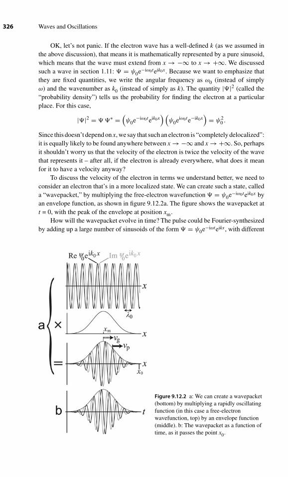
326 Waves and Oscillations
OK, let’s not panic. If the electron wave has a well-defined k (as we assumed inthe above discussion), that means it is mathematically represented by a pure sinusoid,which means that the wave must extend from x → −∞ to x → +∞. We discussedsuch a wave in section 1.11: � = ψ0e−iω0teik0x. Because we want to emphasize thatthey are fixed quantities, we write the angular frequency as ω0 (instead of simplyω) and the wavenumber as k0 (instead of simply as k). The quantity |�|2 (called the“probability density”) tells us the probability for finding the electron at a particularplace. For this case,
|�|2 = � �∗ =(ψ0e−iω0teik0x
) (ψ0eiω0te−ik0x
)= ψ2
0 .
Since this doesn’t depend on x, we say that such an electron is “completely delocalized”:it is equally likely to be found anywhere between x → −∞ and x → +∞. So, perhapsit shouldn’t worry us that the velocity of the electron is twice the velocity of the wavethat represents it – after all, if the electron is already everywhere, what does it meanfor it to have a velocity anyway?
To discuss the velocity of the electron in terms we understand better, we need toconsider an electron that’s in a more localized state. We can create such a state, calleda “wavepacket,” by multiplying the free-electron wavefunction � = ψ0e−iω0teik0x byan envelope function, as shown in figure 9.12.2a. The figure shows the wavepacket att = 0, with the peak of the envelope at position xm.
How will the wavepacket evolve in time? The pulse could be Fourier-synthesizedby adding up a large number of sinusoids of the form � = ψ0e−iωteikx, with different
Figure 9.12.2 a: We can create a wavepacket(bottom) by multiplying a rapidly oscillatingfunction (in this case a free-electronwavefunction, top) by an envelope function(middle). b: The wavepacket as a function oftime, as it passes the point x0.

Chapter 9 ■ Traveling Waves 327
k’s (and corresponding ω’s) for each sinusoid. Each of these sinusoids propagates at
the speed given by equation (9.12.5), vp = hk
2m, so we can propagate each sinusoid
forward in time, and then add them up to see how the wavepacket has propagated. Wewill show that, if we use an envelope which varies slowly enough, then, over short tomoderate time intervals, the envelope propagates without changing its shape, at a speedvg (called the “group velocity”) which matches that of the electron itself. (This means,of course, that the group velocity is different from the phase velocity vp.) This idea ofgroup velocity is critically important for all types of waves governed by a nonlineardispersion relation.
Figure 9.12.2a shows the wavepacket as a function of x. If instead we considerthe behavior as a function of time as the pulse passes the point x0, the plot of � versustime would look as shown in figure 9.12.2b. For the rest of this section, we will thinkprimarily in terms of the dependence on time, instead of the dependence on x.
We will set aside this electron wavepacket for now, but come back to it after we’vefigured out how to calculate the group velocity. For now, let’s consider a differentexample for which the ideas of dispersion and group velocity are important; we’lluse this example as a basis for explicitly showing that the envelope can propagatewithout changing its shape, even for a system with a nonlinear dispersion relation. Ourexample is the important problem of sending information through a fiber optic cable.For example, figure 9.12.3 shows the voltage output from a microphone as I speakthe word, “Hi!.” The horizontal axis is in seconds, so that the entire word lasts about1/4 second. The first part of this is the “H” sound; if you look carefully, you can seea repeating pattern in this part, one copy of which is highlighted with a box. You cansee a different repeating pattern in the last part of the word, which is the “i” sound.The highlight box is 10-ms wide, and the sharpest features in it are perhaps 0.5-mswide. We can see that, later on in the word, there are even sharper features that areabout 0.1-ms wide. So, to Fourier synthesize this waveform, we’d need sinusoids with
frequencies from about1
0.25 sto about
1
0.1 msm, or about 4 Hz to 10 kHz. This is
a typical range for audio signals. We define the function shown in figure 9.12.3 tobe f (t).
Figure 9.12.3 The word “Hi!” as recorded with a microphone. The vertical axis is proportionalto the variation in air pressure relative to background, while the horizontal axis is time in s.

328 Waves and Oscillations
Say that we’d like to send this word over a fiber optic cable. We will study fiberoptics in more detail in section 10.9, but just from the name you can tell that they’reintended to transmit optical signals, that is, signals with frequencies from about 1014
to 1015 Hz. As we discussed earlier, the frequencies in our audio signal f (t) only go upto about 10 kHz, so if we converted the signal to an em wave, it wouldn’t be able topropagate through the fiber optic. One solution is to use the audio signal to “modulate”a fixed-frequency “carrier wave,” that is, to use f (t) as an envelope function for a puresinusoid:
y (t) = f (t)︸︷︷︸envelopefunction
cos ωct︸ ︷︷ ︸carrierwave
(9.12.6)
where the angular frequency ωc of the carrier is in the frequency range that canpropagate through the fiber optic. This idea is illustrated in figure 9.12.4.
To begin with, instead of the complicated f (t) that represents the “Hi!” sound,let’s use a pure sinusoid as the audio signal that is to be transmitted:
f (t) = B cos ωat,
where ωa is an audio frequency, perhaps 2π · 10 kHz, and B is the amplitude. Thus,
y (t) = B cos ωat cos ωct.
Recall from our discussion of beats equation (5.1.3):
A cos ω1t + A cos ω2t = 2A cos ωet cos ωavt,
where, from equation (5.1.2),
ω1 = ωav + ωe and ω2 = ωav − ωe.
Figure 9.12.4 A part of an audio waveform (black) is used as an envelope function for arapidly oscillating carrier wave.

Chapter 9 ■ Traveling Waves 329
Figure 9.12.5 A rapidlyoscillating carrier wavemultiplied by a simple
sinusoidal envelope functionis equal to the sum of two
sinuoids, each at an angularfrequency close to that
of the carrier.
To apply this to our case, we make the following subsitutions: 2A → B, ωe → ωa, andωav → ωc. Therefore,
ω1 = ωc + ωa and ω2 = ωc − ωa, (9.12.7)
⇒ ωc = ω1 + ω2
2and ωa = ω1 − ω2
2, (9.12.8)
and y (t) = B cos ωat cos ωct = B
2cos ω1t + B
2cos ω2t. (9.12.9)
This relation, shown graphically in figure 9.12.5, says that by using the audio signalas an envelope function for the carrier wave, we shift the frequency up close to ωc.(For a fiber optic, ωc ∼ 2π
(1014 Hz
), while ωa ∼ 2π
(104 Hz
), so ωc ± ωa is very
close to ωc in percentage terms.) So, we can now transmit the signal through thefiber optic.15
The glass from which the fiber optic is made has a nonlinear dispersion relation,so we must inquire whether the shape of the envelope function is preserved as thewave propagates. So far, we’ve only been considering the wave as a function of time.To change it to a propagating wave, we replace ω1t by k1x − ω1t, where k1 is thewavenumber corresponding to ω1, and we replace ω2t by k2x − ω2t. Applying this
15. This is essentially how AM (“amplitude modulation”) radio works, but the carrier is a radio wavewith ωc ∼ 2π
(106 Hz
).

330 Waves and Oscillations
recipe to equation (9.12.9), and using equation (9.12.8) gives
y (x, t) = B cos
[(k1x − ω1t
) − (k2x − ω2t
)2
]cos
[(k1x − ω1t
) + (k2x − ω2t
)2
]
= B
2cos
(k1x − ω1t
) + B
2cos
(k2x − ω2t
). (9.12.10)
We will assume that the slope of the function ω (k) is approximately constant over therange ω1 to ω2, so that the wavenumber of the carrier wave is equal to the average ofk1 and k2:
kc = k1 + k2
2. (9.12.11)
We also define
kd ≡ k1 − k2
2. (9.12.12)
Using these, together with equation (9.12.8), we can simplify equation (9.12.10) to
y (x, t) = B cos(kdx − ωat
)︸ ︷︷ ︸envelope function
cos(kcx − ωct
)︸ ︷︷ ︸carrier wave
= B
2cos
(k1x − ω1t
) + B
2cos
(k2x − ω2t
). (9.12.13)
We see that the envelope function travels at the speed vg = ωa
kd= ω1 − ω2
k1 − k2. Recall
that we assume that the slope of the function ω (k) is approximately constant over therange ω1 to ω2, therefore
vg = dω
dk
∣∣∣∣kc
. (9.12.14)
Group velocity (the velocity of the envelope for a wave packet)
In appendix B, it is shown that these ideas all work equally well for a morecomplicated envelope function f (t), rather than the simple sinusoid we used. If f (t)can be Fourier synthesized from sinusoids with angular frequencies from 0 up to ωm,then y (t) = f (t) cos ωct is shown in the appendix to have Fourier components withangular frequencies from ωc − ωm to ωc + ωm. The corresponding traveling wave isshown to have an envelope whose shape is determined by f (t), which travels at thegroup velocity (9.12.14):
y (x, t) = carrier wave︸ ︷︷ ︸travels atvp= ωc
kc
· envelope︸ ︷︷ ︸shape determinedby f (t), travels at
vg≡ dωdk
∣∣∣kc

Chapter 9 ■ Traveling Waves 331
Figure 9.12.6 An example of an envelope modulating a carrier for a travelling wave.
(To obtain the above, we again require thatdω
dkbe constant over the range ωc − ωm to
ωc + ωm.) An example is shown in figure 9.12.6.
To recap:
If we start with an envelope function f (t) having nonzero Fourier components from 0to ωm, and multiply it by a carrier wave cos ωct:
1. The resulting wavepacket y (t) = f (t) cos ωct has Fourier components withangular frequencies from ωc − ωm to ωc + ωm.
2. Ifdω
dkis constant over the range ωc − ωm to ωc + ωm, then the envelope of
the wavepacket doesn’t change shape, and propagates at the group velocity
vg ≡ dω
dk
∣∣∣∣kc
.
3. The peaks and valleys of the carrier wave (which is modulated by the envelope)
propagate at vp = ωc
kc.
Does the idea of group velocity solve the conundrum about electron waves? Let’scheck to see whether the group velocity for a localized electron wavepacket equals thevelocity of the electron itself:
ω = hk2
2m⇒ vg ≡ dω
dk= 2hk
2m= p
m= mve
m= ve
√(Phew!!)
In general, vg can be equal to, greater than, or less than vp. It even occurs in somereal systems that vg is negative, even though all the Fourier component waves havepositive vp!

332 Waves and Oscillations
Figure 9.12.7 A hypothetical dispersionrelation.
Concept test (answer below16): For the hypothetical dispersion relation shown infigure 9.12.7 here, identify (a) a point where vp = vg, (b) a point where vp < vg, (c) apoint where vp > vg > 0, and (d) a point where vp > 0 > vg.
Concept and skill inventory for chapter 9
After reading this chapter, you should fully understand the following
terms:
Traveling wave (9.1)Partial derivative (9.2)The wave equation (9.2)Superposition principle for traveling waves (9.4)Plane wave (9.5)
16. vp ≡ ω/
k is the slope of a straight line drawn from the origin to a point on the dispersion curve,
while vg ≡ dω/
dk is the slope of the curve itself. Therefore, as shown in figure 9.12.8, at point 1they are equal. At point 2, vp > vg > 0. (The group velocity is only slightly positive at point 2.)At point 3, vp < vg. At point 4, vp > 0 > vg.
Figure 9.12.8 Solution to concept test.

Chapter 9 ■ Traveling Waves 333
Poynting vector (9.5)Momentum wave (9.5)Dielectric constant (9.6)Permittivity (9.6)Magnetic susceptibility (9.6)Permeability (9.6)H (9.6)Transmission line (9.7)Displacement wave for sound (9.8)Velocity wave for sound (9.8)Bulk modulus (9.8)Adiabatic (9.8)Continuity equation (9.8)Euler’s equation for fluids (9.8)rms amplitude (9.10)dB (9.11)Dispersion relation (9.12)Carrier wave (9.12)Group velocity (9.12)
You should know what happens when:
Two waves “collide” (9.4)Two equal amplitude sinusoidal traveling waves going in opposite directions are
superposed (9.4)
You should understand the following connections:
Phase velocity, angular frequency, & wavenumber (9.3)Traveling waves & standing waves (9.4)Magnitudes of electric & magnetic fields for em waves in vacuum (9.5)Directions of E, B, & S for em waves (9.5)y, B, H, I, & v (9.5–9.8)FL, E, V , & P′ (9.5–9.8)μ, μ0, μ , L0, & ρ0(9.5–9.8)T , 1/ε0, 1/ε , 1/C0, & γ P0 (9.5–9.8)H & B (9.6)Maxwell’s equations in vacuum & in linear materials (9.6)Density, pressure, displacement, & velocity components of a sound wave (9.8)Fundamental frequency for a wind instrument, length of the air column, speed of sound,
whether one or both ends are open (9.9)Nodes in the pressure wave & antinodes in the displacement wave for a wind
instrument (9.9)rms amplitude & average value (9.10)Graph of the dispersion relation, group velocity, & phase velocity (9.12)

334 Waves and Oscillations
You should understand the differences between:
The functional forms of left- & right-traveling waves (9.2)v & vs (9.8)Power & intensity (9.10)
You should be familiar with the following additional concepts:
The two quantities isomorphic to E and B are in phase for right-traveling waves andout of phase for left-traveling waves. (9.5)
The energy, power, or intensity is proportional to amplitude.2 (9.10)
You should be able to:
Take a partial derivative. (9.2)Test a proposed solution to a differential equation involving partial dervatives. (9.2)Recognize an isomorphism based on (9.5.8) and either (9.5.9) or (9.5.14).Use isomorphisms to quickly copy results for em waves in vacuum to other
systems (9.5–9.8)Calculate the speed of sound for a gas, liquid, or solid (9.8)Calculate the resonant frequencies for a wind instrument with one or both ends
open (9.9)Convert between dB and power or amplitude ratios (9.11)Calculate the group velocity from the dispersion relation (9.12)Explain the difference between the group velocity and the phase velocity (9.12)
In addition to all of the above, you should be able to combine the concepts
you’ve learned to address new situations.
Problems
Note: Additional problems are available on the website for this text.
Instructor: Ratings of problem difficulty, full solutions, and important additionalsupport materials are available on the website.
9.1 (a) Use the fact that any right-travelling wave can be expressed as y (x − vt)
to show that y = −v∂ y
∂ xfor a right-traveling wave.
(b) Use the fact that any left-travelling wave can be expressed as y (x + vt)
to show that y = v∂ y
∂ xfor a left-traveling wave.
9.2 The left end of a long rope with μ = 0.1 kg/m and T = 50 N is moved inthe pattern shown in figure 9.P.1, creating a pulse which then propagates tothe right along the rope. The left end of the rope is at x = 0. Make a sketchof the rope from 0 to 20 m at t = 0.50 s. On your sketch, label the widthand height of the pulse quantitatively, as well as the position of the leftmostpoint on the pulse.

Chapter 9 ■ Traveling Waves 335
Figure 9.P.1 The left end of a rope ismoved in the pattern shown here.
9.3 In a region of outer space, the electric and magnetic fields are described by
E (x, y, z, t) = E0 sin (kx − ωt) j B (x, y, z, t) = B0 sin (kx − ωt) k
The electric field magnitude is greater than zero for 0 < x < 0.4 m, goes tozero at x = 0.4 m, and is negative for 0.4 m < x < 0.8 m.
(a) Using the convention that the length of the vector indicates thestrength of the field, sketch the electric and magnetic fields for pointsalong the x-axis from the origin to x = 1.6 m, at t = 0. Label yoursketch quantitatively.
(b) In which direction is the wave propagating? Explain how youcan tell.
(c) What is the value of k?(d) What is the value of ω?(e) If E0 = 5 × 10⁻⁵ N/C, what is the value of B0?(f) Consider the following four points, with coordinates (x, y, z)
measured in meters: Point 1: (1, 0, 0). Point 2: (1, 0, 1). Point 3:(1.1, 0, 1). Point 4: (1.1, 0, 0). At t = 0, rank the electric field atthese points from largest to smallest. If the field is zero at any point,state that explicitly. If the field is equal at two or more points, statethat explicitly.
(g) Now, make a similar ranking for the magnitude of the magnetic fieldat points 1-4.
(h) Now consider the following other points (again with dimensions inmeters): Point 5: (1, 1, 1). Point 6: (1, −1, 1). Point 7: (1, −1, −1).Point 8: (1, 1, −1). Specify the strength and direction of the electricand magnetic fields at each of these points at t = 0.
(i) A completely different wave is also sinusoidal, and also hasmagnetic and electric fields that depend only on x and t. At t = 0,the magnetic field at the origin is B0 j and the electric field at theorigin is E0k, where B0 and E0 are both positive. In which directionis the wave propagating? How can you tell?
9.4 A wave pulse is traveling to the right on a rope with μ = 0.100 kg/m andT = 20.0 N. The pulse consists of two straight sloping sections, with a sharppeak at the center. (To the left of the peak, the rope has a positive slope, andto the right of the peak it has a negative slope.) Both sloping sections are atangles of 30
◦relative to the horizontal. The peak height is 3.00 cm. Make a

336 Waves and Oscillations
sketch showing the transverse velocity (i.e., the velocity in the y-direction)along the length of the rope, and label your sketch quantitatively, includingthe numerical value for the maximum velocity.
9.5 From the isomorphism between rope waves and em waves in a vacuum,
we have that vp =√
T
μis isomorphic to c = 1√
μ0 ε0. We cannot tell from
this what the individual isomorphisms are between the quantities T and μ
on one hand and the quantities μ0 and ε0 on the other. However, since μ
is associated with the momentum μy (which is isomorphic to B) and μ0 isassociated with B, one might expect that μ might be isomorphic to μ0. Thiswould then require that T is isomorphic to 1/ε0, which makes sense, sinceT is associated with the force from the left (which is isomorphic to E ), andε0 is associated with E. Note that we have not proved this isomorphism.However, check it by applying it to the Poynting vector for an em wave invacuum. What should this translate into for a rope wave? Does it translatecorrectly?
9.6 For an em plane wave in vacuum, assume that E is parallel to j and B is
parallel to k.ApplyAmpère’s law∮
B · d⇀
� = μ0 Inetthreading
+μ0ε0d
dt
∫E · n dA
to a rectangular loop in the x − z plane to show that∂B
∂x= −μ0ε0
∂E
∂ t. This
is equation (9.5.9) that we used to derive the wave equation for em waves.Hint: The derivation of the above equation is essentially the same as thederivation of equation (9.5.8).
9.7 Circular polarization. (a) The “polarization” of an em wave refers tothe direction of the electric field. Thus, for the em waves we’ve explicitlyconsidered, the polarization is along the y-axis. However, this is not at allrequired. For example, we could have the polarization along the z-axis andstill have a wave propagating in the x-direction. The electric field for such awave would be given by E = E0 cos(kx − ωt) k , where E0 > 0. Explain whythe magnetic field for this wave would be given by B = −B0 cos(kx − ωt) j ,where B0 > 0. (Your explanation need not be very mathematical; you shouldinclude a diagram or two.)For the rest of the problem, consider the following electric field (invacuum):
E = E0 cos(kx − ωt) j + E0 sin(kx − ωt) k
(b) Qualitatively describe the behavior of the above electric field, as seenby an observer at the origin. (Hint: radiation with this type of electric fieldis called “circularly polarized.”) (c) How must k be related to ω? (d) Whatis the magnetic field that must accompany the above electric field? Be sureto specify both the magnitude (in terms of E0 and known constants) asa function of position and time, and the direction, using the unit vectorsi, j, and k. The best way to accomplish both these tasks will be to use aCartesian representation, as I did for E. Explain your reasoning briefly.
Chapter 9 ■ Traveling Waves 337
9.8 Waves in three dimensions. We have seen that waves in a one-dimensionalsystem are described by the wave equation
v2p
∂2y
∂x2= ∂2y
∂ t2,
where y = y (x, t). The function y might describe the displacement of a rope,but we have also seen that this equation describes other types of waves, suchas em waves. We have seen that the solutions of this equation that represent
right-moving waves can be written as y(
x − vp t)
= y
[1
k
(kx − kvp t
)]=
y
[1
k(kx − ωt)
]. Written in this way, we can think of the multiplication by
1
kas part of the action of the function; this means that we could either think
of the generic form of a right moving wave as any function y(
x − vpt)
, or
as any function f(kx − ωt). For example, a right-moving sinusoid can bewritten as f(x, t) = A sin (kx − ωt). This gives a wave with wavenumber k,
wavelength λ = 2π
k, angular frequency ω, and phase velocity vp = ω
k.
For a three-dimensional medium which is isotropic (i.e., in which alldirections are equivalent), the wave equation becomes
v2p
(∂2f
∂x2+ ∂2f
∂y2+ ∂2f
∂z2
)= ∂2f
∂ t2,
where now the “thing that is waving” (perhaps the displacement of the ropeor the electric field) is f (x, y, z, t). We can write this in shorter form byintroducing the “Laplacian” operator (named in honor of P. S. de Laplace):
∇2 ≡ ∂2
∂ x2+ ∂2
∂ y2+ ∂2
∂ z2.
This is also often called “del squared,” since it can be thought of as⇀∇ · ⇀∇,
where⇀∇ is del, also known as the gradient operator:
⇀∇ ≡ i∂
∂ x+ j
∂
∂ y+ k
∂
∂ z.
With this, we can write the three-dimensional wave equation for isotropicmedia as
v2p ∇2f = f .
(a) Show that f (k · r − ω t) is a solution to this equation, where k =kx i + ky j + kzk is the three-dimensional version of the wavenumber,
and is called the “wave vector.” (Of course, r = x i+y j+ z k.) In theprocess, find the relation between kx , ky , kz , ω, and vp.
(b) Describe qualitatively what the components of k represent. Hint:Consider the limiting cases when one of the three is equal to 1 m−1,and the other two equal zero.
9.9 Phase relationships for left-traveling sound waves. In section 9.8, weshowed that, for a right-traveling sound wave, the pressure, density, and

338 Waves and Oscillations
velocity are all in phase, while the displacement is 90◦
out of phase withthem. What are the phase relationships between these four components ofthe wave for a left-traveling wave?
9.10 Standing waves of sound. We know that we can create a standing wave bysuperposing left- and right-traveling waves of equal amplitudes.
(a) Superpose two traveling displacement waves of amplitudeδ0
2to
show that the displacement and velocity components of a standingwave of sound are given by
δ = δ0 sin kx cos ωt and v ≡ ∂δ
∂t= −δ0ω sin kx sin ωt.
(b) For a standing wave that is one wavelength long, sketch δ at t = 0,and indicate the displacement vectors in a way similar to the vectorsshown in figure 9.8.1. From your sketch, explain why the densitywave must be ρ′ = −ρm cos kx cos ωt.
(c) Recalling that the potential energy is associated with the pressurewave, which is always in phase with the density wave, explain whyyour results mean that at the time when the kinetic energy of thestanding wave is maximized, the potential energy is zero, and viceversa.
9.11 Potential energy in sound waves. The potential energy of a sound wavedepends on the pressure. At the time of maximum pressure amplitude fora standing wave, the distribution of pressure over a wavelength is exactlythe same as it is over a wavelength of a traveling wave. Therefore, thepotential energy of one wavelength’s worth of a standing wave is the sameas the potential energy of one wavelength’s worth of a traveling wave. Inproblem 9.10, you can show that the kinetic and potential energies for astanding wave of sound are out of phase, that is, that at the time whenthe kinetic energy of the standing wave is maximized, the potential energyis zero, and vice versa. By conservation of energy, this means that themaximum kinetic energy of one wavelength’s worth of a standing waveequals the maximum potential energy, which by the above reasoning equalsone wavelength’s worth of a traveling wave’s potential energy. (a) Foran air tube of length L and cross-sectional area A that is closed at bothends, the standing wave in the velocity would be (see problem 9.10)v = −δ0ω sin kx sin ωt = −v0 sin kx sin ωt, where v0 is the amplitude of thevelocity wave. Use this to show that, for the mode with λ = L, the maximumkinetic energy of the air tube is Kmax = 1
4ρ0Av20 L. Hint: Start by dividing
the tube into slices of infinitesimal thickness dx along the length of the tube,and finding the maximum kinetic energy dKmax of a slice.(b) Explain why this means that the average potential energy intensity of atraveling sound wave is
⟨SU
⟩ = 14 vsρ0v2
0.9.12 Make yourself a mug of hot cocoa. Holding the mug by the handle, stir the
cocoa vigorously, then use your spoon to tap–tap–tap on the rim of the mug.You should hear a musical pitch that changes over time.You can stir the cocoa

Chapter 9 ■ Traveling Waves 339
again and repeat the experiment. (If you are unable to do this yourself, youcan watch a video of me doing it by going to the entry for this problem on thewebsite for this text. However, it’s a lot more fun to do it yourself.) Explainqualitatively what’s going on.
9.13 Is each of the following statements true or false? If true, explain briefly. Iffalse, briefly explain why, and provide a corrected version that is not simplya negation of the original.
(a) In a vacuum, em radiation is carried in both the magnetic and electricfields. The amount of energy carried in the electric field is sometimesmore (and therefore sometimes less) than the amount carried in themagnetic field.
(b) If the electric field points along the −y axis and the magnetic fieldpoints along +z axis, then the Poynting vector (which shows thedirection of wave propagation) points along the −x axis.
(c) Since we can superpose a left-moving wave with a right-movingwave to create an expression for a standing wave, we can alwaysexpress any traveling wave as the sum of two or more standingwaves.
(d) An em wave is traveling in a linear material. When it entersa different material that has the same permeability but a largerpermittivity, its velocity increases.
9.14 Power in transmission line waves. From the isomorphism between trans-mission line waves and em waves in vacuum, we have that L0C0 isisomorphic to μ0 ε0. We cannot tell from this what the individual isomor-phisms are between the quantities L0 and C0 on one hand and the quantitiesμ0 and ε0 on the other. However, since L0 is associated with the current(which is isomorphic to B/μ0), and μ0 is associated with B, one mightexpect that L0 might be isomorphic to μ0. This would then require C0 isisomorphic to ε0, which makes sense since C0 is associated with the voltage(which is isomorphic to E ), and ε0 is associated with E. Check this proposedisomorphism by applying it to the Poynting vector for an em wave in vacuum.What should this translate into for a waves on a transmission line? Does ittranslate correctly?
9.15 Power in a rope wave. A traveling rope wave carries both kinetic andpotential energy. In this problem, you will find the total power carried by thewave. Consider a sinusoidal wave traveling to the right y = A cos(kx − ωt).The rope has tension T and mass per unit length μ.
(a) Show that the kinetic energy in one wavelength’s worth of this waveis 1
4λμA2ω2. Hint: you may as well make the calculation at t = 0.Also, recall that the average value of the square of a sinusoid is 1/2 .
(b) Calculating the potential energy for a traveling wave is moredifficult, so we will use a trick. The potential energy is determinedby the shape, and the shape of one wavelength’s worth of a

340 Waves and Oscillations
traveling wave is the same as one wavelength’s worth of a standingwave (at a moment when the wave is at its maximum amplitude).Therefore, the potential energy of one wavelength’s worth of atraveling wave is the same as the maximum potential energy ofone wavelength’s worth of a standing wave. Explain why this is thesame as the maximum kinetic energy of one wavelength’s worth of astanding wave.
(c) Show that the maximum kinetic energy in one wavelength’s worthof a standing rope wave of amplitude A is 1
4λμA2ω2.(d) Show that the power in a traveling rope wave is P = 1
2μA2ω2vp.
9.16 Completing the isomorphism between sound waves and em waves in
vacuum. For sound waves in a gas, we have vs =√
γ P0
ρ0, which is
isomorphic to c = 1√μ0 ε0
. We cannot tell from this what the individual
isomorphisms are between the quantities γ , P0, and C0 on one hand and thequantities μ0 and ε0 on the other. However, since ρ0 is associated with themomentum-per-volume ρ0 v (which is isomorphic to B), and μ0 is associatedwith B, one might expect that ρ0 might be isomorphic to μ0. This wouldthen require that γ P0 is isomorphic to 1/ε0, which is reasonable since P0is associated with the pressure variation (which is isomorphic to E ), andε0 is associated with E. By considering the power transmitted in the wave,show that this hunch is correct. Hint: Note that in (9.11.3), 〈S〉 = 1
2 vsρ0v20,
the quantity given is the average intensity.9.17 The 287th Annual Solar System Olympics is being held on Venus, where
conditions are rather different from here. On Earth, the atmospheric pressureis 101.3 kPa. The 100-m dash is held in Sandworm’s Borough Stadium onthe surface of Venus, where the atmospheric pressure is 92 times that of Earthand the atmospheric density is 65 kg/m3. The atmosphere is mostly CO2,and is at a temperature of 400
◦C. Assume the adiabatic index (γ ) of this
atmosphere is 1.235. The starter, standing at the start line, fires the startingpistol.
(a) How long will it take for the sound of the gun going off to reach atimer standing at the finish line?
(b) What is the rms amplitude of pressure in the sound wave that comesout of the barrel of the gun, if the sound intensity measured rightnext to the muzzle is 140 dB?
(c) After a blistering 8.69 s, a human crosses the finish line ahead ofall of the other competitors. We are now at the medal ceremony,and the Aphrodite Orchestra is playing Joe Diffie’s “Third Rockfrom the Sun,” the planetary anthem of Earth. The flautist, whohappens to be from Pluto, has placed an extension onto the end ofher flute to take into account the atmospheric conditions on Venus.Assuming the conditions from part a still apply, how long must theflute become if the flute is tuned so that its first harmonic occurs

Chapter 9 ■ Traveling Waves 341
at 880 Hz? How long must a clarinet be if it were to fit the samecharacteristics?
9.18 A wave y1 = A cos(k1x − ω1t) is superposed with a wave y2 = Acos(k2x − ω2t), where k1 is fairly close to k2. (a) What is the group velocity ofthe resulting waveform, that is, the velocity of the envelope? (b) What is thewavelength of the rapidly oscillating function contained within the envelope?(c) What is the speed of the crests of the rapidly oscillating function?
9.19 A Gaussian wavepacket of light travels through a sheet of glass whichhas a nonlinear dispersion. Explain what is wrong with the followingstatement: “When the wavepacket emerges from the glass, the high-frequency components are shifted to the front of the packet, and thelow-frequency components are shifted to the back.”
9.20 For waves in deep water (depth at least as large as the wavelength), withamplitude much less than the wavelength, the dispersion relation is ω2 =gk + γ k3
ρ. The gk part of this dominates at small k (i.e., at large wavelength),
and describes the situation when the restoring force is provided by gravity(g is the acceleration of gravity). Waves in this regime are called “gravity
waves.” Theγ k3
ρdominates at large k, and describes the situation when
the restoring force is provided by surface tension; γ is the surface tension(7.2 × 10⁻² N/m for pure water), and ρ is the density (1,000 kg/m3). Wavesin this regime are called “capillary waves.” (a) At what wavelength do thesetwo terms make equal contributions? (b) Use a graphing program to makea plot of ω as a function of k for wavelengths ranging from 5 mm to 20 cm.On the same graph show separate curves for pure gravity waves and purecapillary waves as dashed lines, and label each of the three curves. (c) Forgravity waves (waves with a wavelength long enough that surface tensioneffects are negligible), what is the phase velocity in terms of g and k? (d) Forgravity waves, show that the group velocity for waves having wavenumbersin a range centered on k is half the phase velocity. (e) For capillary waves(which have a wavelength short enough that the gk term can be ignored),what is the phase velocity in terms of k, γ , and ρ? (f) For capillary waves,show that the group velocity for waves having wavenumbers in a rangecentered on k is 3/2 the phase velocity.
9.21 Em waves in the ionosphere. (This is an example of a problem that looksmuch more intimidating than it really is.) So far, we have considered emwaves in vacuum. One of the layers of the Earth’s atmosphere is made ofmostly ionized gas, and is called the “ionosphere.” It is responsible for long-range transmission of AM radio, since the radio waves bounce off this layerand then back down to Earth. Suppose that em waves in the ionosphere aregoverned by the following differential equation:
∂2E
∂t2= c2 ∂2E
∂x2− ω2
0E,

342 Waves and Oscillations
where c and ω0 are known constants. You are told that all possible solutionsof this equation can be expressed in the form
E (x, t) =∞∫
−∞ε (k) ei(kx−ωt)dk,
where ε (k) is a function of k.
(a) A naïve student might think that the above could only representright-moving waves. Explain why this is incorrect.
(b) Given that the above is a solution to the differential equation, whatmust be the dispersion relation? Hint: rearrange the differentialequation so that you have zero on one side. Then, bear in mind thatintegrating with respect to k commutes with taking the derivativewith respect to x or t. Finally, if you can make the integrand zero,then the integral will definitely be zero.
(c) A burst of sine waves with a small range of angular frequenciescentered on ω1 is emitted from the point x = 0. The burst has aduration τ . Approximately how long will it take the burst to reachthe point x = L?

10 Waves at Interfaces
Come with me if you want to live!—Arnold Schwarzenegger as the Terminator in Terminator 2: Judgment Day
So far, we have discussed waves traveling through an unchanging medium. However,interesting and surprising things happen at the interface between two differentmediums, leading to a wealth of important science and applications. In this chapter,we begin by studying the behavior of wave pulses on ropes when they encounter aboundary at which the mass/length of the rope suddenly changes. Although this maynot sound very exciting, bear in mind that waves on a rope are exactly analogous towaves in any elastic medium. Therefore, for example, by understanding how transversewaves on a rope behave, we immediately discover the behavior for torsional wavesin solids. For learning purposes, waves on ropes have the distinct advantage that theyare easily visualized and relatively easy to understand intuitively. Furthermore, themethods we use for determining the behavior of rope waves at interfaces are almostexactly the same as those you will use in a future course to understand the behavior ofquantum waves at interfaces, a most important problem indeed. We will also explicitlydiscuss the behavior at interfaces of sound waves, waves on transmission lines, andelectromagnetic waves in a vacuum. The work we do with rope waves will serve uswell when we reach these other, perhaps more interesting, types of waves, since wewill again find isomorphisms for the behavior at interfaces.
10.1 Reflections and the idea of boundary conditions
In section 1.11, we discussed the simplest type of quantum mechanical wave,� (x, t) =ψ0e−iωteikx. We showed that an electron described by such a wave function iscompletely delocalized, that is, it is equally probable to be found at any point in space.Often, we are interested in electrons which are more localized; a possible wavefunctionfor such an electron is shown schematically in figure 10.1.1a. (Recall that the quantummechanical wavefunction is inherently complex; only the real part is shown in thefigure.) This “wave packet” is travelling in a region of constant potential energy U,but is about to encounter a place where U suddenly increases. We will not treat this
343

344 Waves and Oscillations
Figure 10.1.1 A Quantum mechanicalwavepacket approaching a place wherethe potential energy suddenly changes(a) is analogous to a rope wavepacketapproaching a place where themass/length suddenly changes (b).
problem quantitatively in this book, but it is quite analogous to the problem of a wavepacket on a rope wave shown in figure 10.1.1b.
At the moment shown, the wave packet (or pulse) is traveling on a rope withlow mass/length μ1, and is about to encounter an interface at which the mass/lengthsuddenly increases to a larger value μ2. (The tension is the same in the two parts of therope.) For now, we assume that any conversion of the energy in the wave into thermalenergy is negligible. We then recognize that some of the energy in the pulse might betransmitted into the heavier part of the rope as a pulse traveling further to the right, butsome might also be reflected as a pulse traveling to the left in the lighter part of therope. Our job is as follows: given the shape of the incident pulse, find the shape of thetransmitted and reflected pulses. We define the following:
Table 10.1.1. Functions for rope waves
R1(x − v1t) Function describing the incident pulse, which travels to the right in medium 1(the left part of the rope).
L1(x + v1t) Function describing the reflected pulse, which travels to the left in medium 1.R2(x − v2t) Function describing the transmitted pulse, which travels to the right in medium 2
(the right part of the rope).
We want to describe things for all times, including the time before the pulseencounters the interface, the time during the encounter, and the time after the encounter.During the encounter, the left part of the rope has both the tail end of the pulse (movingright) and also the front end of the reflection (moving left). So, in general, the motionof the rope to the left of the interface (medium 1) is
y1 (x, t)︸ ︷︷ ︸motion ofmedium 1
= R1
(x − v1t
)︸ ︷︷ ︸incident,
right-movingwave
+ L1
(x + v1t
)︸ ︷︷ ︸reflected,
left-movingwave
, (10.1.1)

Chapter 10 ■ Waves at Interfaces 345
while the motion of the rope to the right of the interface (medium 2) is
y2 (x, t)︸ ︷︷ ︸motion ofmedium 2
= R2
(x − v2t
)︸ ︷︷ ︸transmitted,
right-movingwave
. (10.1.2)
So, given the function R1, our task is to find L1 and R2. In this section, we’ll find L1.The properties of medium 1 determine how fast pulses travel, but place no
constraint on the shape of the pulse. Similarly, the properties of medium 2 determineonly the speed of waves in that medium. So, the details of L1 and R2 must be determinedby the properties of the interface itself, combined, of course, with the details of R1.There are two important properties of the interface; these are referred to as “boundaryconditions”:
1. At the interface, the rope must be continuous. We set x = 0 at the interface, sothis condition is
y1 (0, t) = y2 (0, t) (10.1.3)
⇒ [R1 + L1
]x=0 = R2
∣∣x=0 .
Taking the time derivative of this gives[∂R1
∂t+ ∂L1
∂t
]x=0
= ∂R2
∂t
∣∣∣∣x=0
. (10.1.4)
2. Figure 10.1.2 shows the interface at a time when the pulse is passing through it.We consider an infinitesimal segment of the rope, at the interface. This segmenthas infinitesimal mass. Therefore, to avoid infinite acceleration, the net forceapplied to it must be zero. It experiences a force T2 from the right part of therope and a force T1 from the left part. For these forces to cancel, they mustpoint in opposite directions. Since the tension force in a rope points along therope, this means that
∂y1
∂x
∣∣∣∣x=0
= ∂y2
∂x
∣∣∣∣x=0
(10.1.5)1
⇒[
∂R1
(x − v1t
)∂x
+ ∂L1
(x + v1t
)∂x
]x=0
= ∂R2
(x − v2t
)∂x
∣∣∣∣∣x=0
. (10.1.6)
Since R1 is a function of the combination(x − v1t
), we have that
∂R1
(x − v1t
)∂x
= ∂R1
(x − v1t
)∂(−v1t
) . (10.1.7)
1. The same combination of boundary conditions, that is, continuity of the wavefunction (10.1.3)and continuity of its derivative (10.1.5) are used to solve the equivalent problem in quantummechanics.

346 Waves and Oscillations
Figure 10.1.2 Top: Forces on an infinitesimal segment of rope at the interface must cancel, toavoid infinite acceleration. Bottom: As we’ll see later in this chapter, reflection of light off thesurface of water is closely analogous to reflection of rope waves off the interface between alight rope and a heavy one. This shows the 3rd Avenue bridge in Minneapolis. Image ©Geoffrey Kuchera | Dreamstime.com
Now, we use the chain rule:
∂R1
(x − v1t
)∂(−v1t
) = ∂R1
(x − v1t
)∂t
dt
d(−v1t
) = ∂R1
(x − v1t
)∂t
(d(−v1t
)dt
)−1
= − 1
v1
∂R1
(x − v1t
)∂t
.
Combining this with equation (10.1.7) gives
∂R1
(x − v1t
)∂x
= − 1
v1
∂R1
(x − v1t
)∂t
.
Applying this, and the analogous expressions for R2 and L1 to equation (10.1.6) yields
⇒[− 1
v1
∂R1
∂t+ 1
v1
∂L1
∂t
]x=0
= − 1
v2
∂R2
∂t
∣∣∣∣x=0
.

Chapter 10 ■ Waves at Interfaces 347
Using equation (10.1.4) to substitute for∂R2
∂t
∣∣∣∣x=0
in the above, gives
[− 1
v1
∂R1
∂t+ 1
v1
∂L1
∂t
]x=0
= − 1
v2
[∂R1
∂t+ ∂L1
∂t
]x=0
.
Integrating with respect to time, and multiplying by −v1v2, we obtain[v2R1 − v2L1 = v1R1 + v1L1 + const.
]x=0 ⇔[(
v2 − v1
)R1 = (
v2 + v1
)L1 + const
]x=0 .
This equation must hold true under all conditions. In particular, it must be true whenthe rope is at equilibrium, that is, when R1 = L1 = 0. Therefore, the constant mustequal zero. So, finally, we get [
L1 = R1v2 − v1
v2 + v1
]x=0
. (10.1.8)
Core example: Applying the reflection equation.
We consider the case v1 = 3v2, so that[L1 = −1
2R1
]x=0
. Each part of the incident pulse
causes the corresponding part of the reflected pulse, so that the sequence before andafter the encounter with the interface is as shown in figure 10.1.3a. Note that only thebehavior for x < 0 is shown; in section 10.3, we’ll figure out the behavior for x > 0.
Concept test 1 (answer below2): For the situation shown in the core example above,make a sketch of R1, L1, and y1 for a time during the encounter of the pulse with theinterface, so that the sketch of R1 looks as shown in figure 10.1.3b. At this time, onlyabout the first quarter of the pulse has encountered the interface.
Concept test 2 (answer below3): If we attach the end of a rope to a wall, and launch apulse at this interface (as shown in figure 10.1.5), what does the reflection look like wellafter the encounter of the pulse with the interface? Hint: Think about the wall as if it werea very heavy rope. What is the speed in such a rope?
The opposite limit, of v2 → ∞, is more difficult to contrive. We must attach theleft part of the rope to something that has the same tension, but zero mass. The onlyway to do this is to use a massless ring, which slides without friction on a pole, asshown in figure 10.1.7. This arrangement is obviously a bit ridiculous, but the analogsfor other types of waves are important, and we’ll discuss them later in this chapter.
2. The answer to Concept test 1 is shown in figure 10.1.4.
3. The speed of a rope wave is√
T/μ. We think of the wall as a rope with infinite μ, so that
v2 = 0. Using equation (10.1.8) this gives[L1 = −R1
]x=0, so the reflection is the same size as
the incident pulse, but inverted, as shown in figure 10.1.6.

Figure 10.1.3 a: The behavior ofthe part of the rope to the left ofthe interface for the caseL1 = −R1/2. b: R1 for a time earlyin the encounter of the pulse withthe interface. Don’t look yet at thenext figure.
Figure 10.1.4 The reflection of a pulseduring the encounter with the interface.
Figure 10.1.5 A pulse about to hit a brickwall.
348

Chapter 10 ■ Waves at Interfaces 349
Figure 10.1.6 The reflected pulse wellafter the encounter with the brick wall.
Figure 10.1.7 Reflection of a pulse off amassless ring which slides without
friction on a pole.
In this limit, equation (10.1.8) gives[L1 = R1
]x=0, so that the reflected pulse has the
same amplitude as the incident pulse, and is not inverted.
10.2 Transmitted waves
Imagine you are a dog holding the left end of a rope which is under tension, as shown infigure 10.2.1. Suddenly, you move your head up, launching a right-moving wavefront,as shown.
The same thing happens at the interface, for a rope wave; the motion of the pointat the interface (the left end of the heavy part of the rope) launches the transmittedpulse into the right part of the rope.
Figure 10.2.1 If you suddenly move your head up, you will launch a right-moving wavefront.

350 Waves and Oscillations
In this case, we only need the boundary condition that the rope is continuous atthe interface:
y1 (0, t) = y2 (0, t)
⇒ [R1 + L1
]x=0 = R2
∣∣x=0 .
Your turn: Use this, and the results of section 10.1, to show that[R2 = R1
2v2
v2 + v1
]x=0
. (10.2.1)
Thus, the transmitted wave has an amplitude relative to the incident wave of2v2
v2 + v1. Because it travels at speed v2, it is compressed or expanded in the horizontal
direction by the ratio v2
/v1.
Core example: Shape of the transmitted wave pulse.
Again, we consider the case v1 = 3v2. From equation (10.2.1), we see that R2 = R1
/2.
We launch the same pulse as before toward the interface. As shown in figure 10.2.2a,
the transmitted pulse is scaled by the factor2v2
v2 + v1in the in the y-direction, and by the
factor v2
/v1in the x-direction.
Concept test (answer below4): Sketch R1, R2, L1, y1, and y2 at the point in time whenthe first quarter of the pulse has encountered the interface, that is, at the time shown infigure 10.2.2b. Make your sketch as quantitative as possible.
Self-test (answer below5): Now, let v1 = 13
v2, so that the left side of the rope is heavier.
Use the same incident pulse as is shown in figure 10.2.2. Sketch R1, R2, L1, y1, and y2 fora point in time well after the pulse has encountered the interface. Make your sketch asquantitative as possible.
Sinusoidal waves are particularly important, partly because any wave can beexpressed as a sum of sinusoids, as we saw in chapter 8. What happens to a sinusoidal
4. The answer to the Concept Test is shown in figure 10.2.3.5. Answer to Self-test: Using equation (10.1.8), the amplitude of the reflected pulse is half
that of the incident pulse, and the reflection is noninverted (i.e., the amplitude is positive).Using equation (10.2.1), the amplitude of the transmitted pulse is 3/2 that of the incident pulse.Because v2 is three times v1, the transmitted pulse is stretched in the horizontal direction bya factor of three. Putting this all together gives figure 10.2.4. It might at first appear that thisviolates conservation of energy, since the transmitted pulse is higher and wider than the incidentpulse. However, since medium 2 is lighter, it takes less energy to create pulses in it.

Chapter 10 ■ Waves at Interfaces 351
Figure 10.2.2 a: An incident pulse (top) is partly transmitted and partly reflected (bottom).Note that the reflected pulse travels three times as fast as the transmitted pulse. b: Onequarter of the way through the encounter. Don’t look yet at the next figure.
Figure 10.2.3 Reflection and transmission of a pulse during the encounter with the interface.
wave when it encounters an interface? As for all other waves, the horizontal scalefor the transmitted wave is changed by the factor v2
/v1, so that the wavelength in
medium 2 is
λ2 = v2
v1λ1. (10.2.2)

352 Waves and Oscillations
Figure 10.2.4 Reflection and transmission for a case where the speed is three times greater onthe right side of the interface.
Does the angular frequency change?
v2 = ω2
k2⇔ ω2 = v2k2 = 2πv2
λ2= 2πv2
v2
v1λ1
= 2πv1
λ1= v1k1 = ω1.
So:
When a sinusoidal wave moves from one medium to another, the wavelength
changes, but the frequency doesn’t change.
We can also see this by considering that each crest of the transmitted wave is launchedby a crest in the incident wave.
10.3 Characteristic impedances for mechanical systems
Concept test (answer below6): We saw in section 10.1 that, when a rope waveencounters a brick wall, it is reflected with full amplitude but inverted. If it insteadencounters a massless ring that slides frictionlessly on a pole, it is reflected with fullamplitude but noninverted. One might expect that there would be some middle groundwhere there is no reflection at all, that is, a condition halfway between an inverted anda noninverted reflection. Perhaps if we attach the rope to a ring that has some carefullychosen mass, and that slides frictionlessly on a pole, we could suppress the reflection.Explain, using fundamental physical principles, why this couldn’t work.
As we saw in chapter 9, transmission lines (such as coaxial cables) can supportelectromagnetic waves, which behave in many ways like waves on ropes. Thus, we
6. The wave pulse carries energy. Since the ring slides frictionlessly, it cannot dissipate the energy,so the only way for energy to be conserved is by generating a reflection.

Chapter 10 ■ Waves at Interfaces 353
Figure 10.3.1 Top: model for a cable TVtransmitter attached to a coaxial cable.
Bottom: schematic for a cable TVnetwork; the lines represent coaxial
cables.
can expect that, when a wave pulse travelling along a coaxial cable reaches the endof the cable, reflections will be generated (just as reflections are generated when apulse reaches the end of a rope attached to a wall or a ring). This could create a veryserious problem for the operator of a cable television system. To broadcast on such asystem, waves are launched into the cable, as shown schematically in the top part offigure 10.3.1. This signal must be sent to many houses, as shown in the bottom part;if reflections are generated at each one, there will be terrible interference problems,dramatically reducing picture quality. What is needed is some way to end the cable (aswe must do at each house) but suppress the reflections. The device attached to the endof the cable that accomplishes this suppression is called a “terminator.”
This is analogous to the problem of suppressing reflections for a rope wave, andthe basic solution is the same in both cases. If instead of ending the cable, we attachedan infinite length of cable of the same type, clearly no reflections would be generated.So, how can we make a compact device that “feels” like an infinite length of cable?For a rope, how can we make a compact device that feels like an infinite length of ropeunder tension?
For the rope, we will borrow an idea from our earlier study of ac circuits, insection 1.10. There, we encountered the generalized version of the resistance, calledthe impedance. This is defined as Z ≡ V /I , where V is the complex version of thevoltage and I is the complex version of the current. For a resistor, we have simplyZ = R; because this is real, the current and voltage are in phase for a resistor. However,
for a capacitor we found that Z = 1
iωC; because this is purely imaginary, the current
and voltage are 90◦ out of phase for a capacitor. One might say that the impedancecharacterizes the way a circuit element “feels.” We will define the equivalent quantityfor a mechanical system, and then show that, if we construct a compact object with thesame impedance it does indeed suppress reflections.
What is the mechanical equivalent of the impedance Z ≡ V /I? Recall theisomorphism between the damped driven mechanical and electrical oscillators:
(4.1.3a) : mx + bx + kx = F0 cos ωdt
(4.6.1) : Lq + Rq + q
C= V0 cos ωdt

354 Waves and Oscillations
So, the voltage is isomorphic with the applied force, and the current (which equals q) isisomorphic with the velocity x. By analogy with Z ≡ V /I , this suggests the followingdefinition of the mechanical impedance:
Z ≡ Fapplied
z, (10.3.1)
Definition of mechanical impedance for a compact object
where Fapplied is the complex version of the applied force (e.g., for the damped driven
oscillator, Fapplied = F0eiωdt) and z is the complex version of the velocity y (e.g., for the
damped driven oscillator in a steady-state, z = d
dt
[Aei(ωdt−δ)
]). If Fapplied is in phase
with the velocity y, then Z is real, just as the impedance is real for an electrical circuitif the voltage is in phase with the current. However, if Z is complex, then Fapplied isnot in phase with y. Since Z may generally be complex, we don’t bother to include thetilde above it.
Self-test (answer below7): For a damped driven harmonic oscillator, what is theimpedance Z? Express your answer in terms of F0, A, δ , and ωd.
For an extended object such as a rope, we must be a bit more careful with ourdefinition. Imagine you are holding the left end of a rope in your hand. You can launchwaves down the rope by moving your hand up and down, exerting a force on the tinypiece of the rope you are actually touching. However, this is not the only force thispiece of rope feels; it also feels a force from the rest of the rope, off to its right. So,because our definition involves the applied force, we could also write it (for the caseof right-moving waves) as the force coming from the left side of a piece of rope:
Z ≡ FL
z,
Definition of mechanical impedance for right-traveling waves
where FL is the complex version of FL (the y-component of the force exerted on apiece of rope from its left end), and z (x, t) is the complex version of the velocity in they-direction, that is, y = Re z. We already know from the arguments of section 9.5 thatFL is in phase with y for a right-moving wave, so Z is real, and we can simply write
Z = FL
y(10.3.2)
Mechanical impedance for right-traveling waves.
7. Answer to self-test: Z =Fapplied
z= F0eiωdt
d
dt
[Aei(ωdt−δ)
] = −ieiδ F0
ωdA= ei(δ−π/2) F0
ωdA. So, when
δ = π/2 (which occurs when ωd = ω0), the impedance is real, meaning that the drive force isin phase with the velocity, as we already knew.

Chapter 10 ■ Waves at Interfaces 355
It is not difficult to calculate Z , since we already know from equation (9.5.15) that
FL = −T∂y
∂x. So, we need to express y in terms of
∂y
∂x, so that when we take the ratio we
will get a constant. For a right moving wave, the solution to the wave equation is of the
form y (x − vt). Therefore, by the chain rule, y = ∂y
∂t= −v
∂y
∂x. (For example, if y =
A sin [k (x − vt)], then∂y
∂t= −kvA cos [k (x − vt)], while
∂y
∂x= kA cos [k (x − vt)].)
Therefore,
Z =−T
∂y
∂x
−v∂y
∂x
= T
v.
From equation (9.2.4), v =√
Tμ
, so that
Zrope = √Tμ (10.3.3)
For a left-traveling wave, the solution to the wave equation is of the form y (x + vt),
so that y = ∂y
∂t= +v
∂y
∂x. Since the impedance should be a property of the rope, and
should not depend on the direction of wave travel, we therefore see that we must alterthe definition (10.3.2) for the case of left-moving waves:
Z = −FL
y.
Mechanical impedance for left-traveling waves.
Just to check: Z = −−T
∂y
∂x
v∂y
∂x
= T
v= √
Tμ, as desired. You may be wondering why, for
left-traveling waves, we don’t instead define Z = +Fr/y , where Fr is the y-componentof force applied to a segment of rope from the right. This would be correct, but it is notas convenient. We wish to build on the isomorphisms developed in chapter 9, whichare all based on FL, so it is better to stick with FL in this chapter as well. Furthermore, itis easier to discuss boundary conditions when we use the same quantity FL to describeleft- and right-traveling waves.
Let us return now to right-traveling waves. If you hold the left end of the rope,the force you apply to it is FL. Because the velocity y is in phase with FL, it is in phasewith the force you apply. Thus, the rope “feels” different from a small rock, for whichthe acceleration is in phase with the force you apply. The difference comes becausethe end of the rope feels not only the force you are exerting now, but also the forcefrom the part of the rope just to its right. That part of the rope is at a position thatis determined by the propagating wave, that is, that is determined by the force youexerted on the end of the rope a short time ago.
So, how can we terminate the rope in such a way as to suppress reflections? Inother words, which compact object has the same impedance as an infinite length ofrope, so that it feels the same as an infinite length of rope? In other words, whichcompact system has a velocity that is in phase with the applied force? The answer

356 Waves and Oscillations
Figure 10.3.2 By connecting a rope to a massless ringimmersed in a suitably chosen damping fluid, we cansuppress reflections.
is a massless ring, sliding on a frictionless pole, and immersed in a viscous dampingmedium. Because the ring is massless, the net force applied to it must be zero (otherwiseits acceleration would be infinite). Therefore, the force applied to it (in this case by therope) must be opposite the damping force, that is,
Fapplied = − (−by) = by, (10.3.4)
so that, as we need, the y-velocity is in phase with the applied force. The impedance ofsuch a ring is the ratio of the force to the velocity, so that Z damped
masslessring
= b, and to suppress
reflections of waves traveling down the rope, we just match impedances (so that thering feels like an infinite rope), that is, we choose the size of the ring and the viscosityof the damping medium so that
b = √Tμ.
One way to accomplish this would be to have the rope be vertical, and the ring beimmersed in a pool of liquid, as suggested in figure 10.3.2. Note that the dampingprovides a way to absorb the energy of incident pulses.
Now, unless you plan to create a telephone company based on tin cans tiedtogether with strings, the previous discussion might seem rather contrived. However, insection 10.4 we will develop the ideas needed to determine reflection and transmissionfor all the types of waves we have studied, making use of the isomorphisms uncoveredin chapter 9. Then, in section 10.5, we apply these ideas to the more practicalconsiderations of how to suppress reflections in transmission lines (such as coaxialcables).
10.4 “Universal” expressions for transmission and reflection
We saw in section 9.5 that the displacement wave y (x, t) is not isomorphic to any of thequantities that characterize other wave types. Instead, the velocity wave y is isomorphicto, for example, B/μ0 for an electromagnetic wave in vacuum, and FL is isomorphicto, for example, the electric field E of an electromagnetic wave in vacuum. We will seethat all these isomorphisms remain faithful when we consider the boundary conditions

Chapter 10 ■ Waves at Interfaces 357
for each of the various types of waves. Therefore, it is worthwhile for us to considerthe reflection and transmission for the y wave and the FL wave. However, for the mostgeneral case we must allow the tension T to be different in the two parts of the rope.To accomplish this, we imagine that the two halves are connected by a massless ringwhich slides frictionlessly on a pole, so that the pole can supply the force needed forthe tensions to be different. To the left of the pole we have rope 1, and to the right wehave rope 2.
What is the boundary condition on FL? Consider the forces exerted on the masslessring. The force exerted on the ring by the section of rope to its left is, of course, FL1,where “1” in the subscript indicates the force is exerted on the left side of the interface.The ring exerts a force FL2 on the rest of the rope to its right, where “2” indicatesthe force is exerted on the right side of the interface. By Newton’s third law, this isopposite to the force exerted by the rope to its right on the ring, so that the net force(in the y-direction) exerted on the ring is FL1 − FL2. Since the ring is massless, the netforce must be zero (otherwise its acceleration would be infinite), so that[
FL1 = FL2
]x=0 . (10.4.1)
Boundary condition for FL
In other words, the boundary condition for FL is that it must be continuous at theinterface.
As we did when considering the displacement y of the rope, we can express FLin rope 1 (to the left of the interface) as the sum of the right-traveling incident waveFL, R1 and the left-traveling reflected wave FL, L1:
FL1 = FL, R1 + FL, L1.
On the right side of the interface, there is only the transmitted wave:
FL2 = FL, R2.
Therefore, the boundary condition becomes[FL, R1 + FL, L1 = FL, R2
]x=0
. (10.4.2)
What is the boundary condition for y? We know that the rope itself must be continuous,that is,
[y1 = y2
]x=0. Taking the time derivative of this gives[
y1 = y2
]x=0 . (10.4.3)
Boundary condition for y
Expressing this in the R1, L1, R2 notation, we have[yR1 + yL1 = yR2
]x=0 . (10.4.4)
We will begin by finding the reflected and transmitted y waves. For notationalconvenience, in what follows we omit the explicit reminders that we are consideringthe behavior at the interface x = 0. Dividing equation (10.4.2) by (10.4.4) gives
FL, R1 + FL, L1
yR1 + yL1= FL, R2
y R2.
358 Waves and Oscillations
From equation (10.3.2), Z2 = FL, R2
yR2, so that above becomes
FL, R1 + FL, L1 = Z2
(yR1 + yL1
). (10.4.5)
From equation (10.3.4), we have that, for the reflected wave (which travels left)
Z1 = −FL, L1
yL1⇔ FL, L1 = −yL1Z1.
Substituting this into equation (10.4.5) gives
FL, R1 − yL1Z1 = Z2
(yR1 + yL1
).
Dividing by yR1 gives
FL, R1
yR1︸ ︷︷ ︸Z1
− yL1
yR1Z1 = Z2
(1 + yL1
yR1
)⇒ Z1 − Z2 = yL1
yR1
(Z1 + Z2
) ⇒
yL1 = yR1Z1 − Z2
Z1 + Z2, or (10.4.6)
[yreflected = yincident
Zi − Zt
Zi + Zt
]x=0
, (10.4.7)
where Zi = Z1 is the impedance for the rope on the incident side and Zt = Z2 is theimpedance for the rope on the transmitted side.
Your turn: Use equation (10.4.6) to substitute for yL1 in equation (10.4.4) and show that[ytransmitted = yincident
2Zi
Zi + Zt
]x=0
, (10.4.8)
Concept test (answer below8): A right-traveling pulse gets to the end of a rope, whichis attached to a massless ring which slides frictionlessly on a pole. Is the reflected y pulseinverted or not with respect to the incident y pulse? Use the results of this section to getyour answer.
For FL, the expressions for reflection and transmission are different. The reflectedwave moves left in rope 1, so
Z1 = −FL, L1
yL1⇔ FL, L1 = −yL1Z1 = −yL1
FL, R1
yR1.
8. The massless ring has zero impedance (since an infinitesimal force in the y-direction is all that’sneeded to produce a velocity and Z = FL
/y). Plugging Z2 = 0 into equation (10.4.6) gives
[yreflected = yincident]x=0, so the reflected velocity pulse is uninverted.

Chapter 10 ■ Waves at Interfaces 359
Using equation (10.4.6) to substitute for yL1, we then have that, at the interface,
FL, L1 = −FL, R1Z1 − Z2
Z1 + Z2or
[FL, reflected = FL, incident
Zt − Zi
Zi + Zt
]x=0
. (10.4.9)
The transmitted wave moves right in rope 2, so
Z2 = FL, R2
yR2⇔ FL, R2 = yR2Z2.
Using (10.4.8) to substitute for yR2, we get that, at the interface
FL, R2 =(
yR12Z1
Z1 + Z2
)Z2.
Using Z1 = FL, R1
yR1⇔ yR1 = FL, R1
Z1, we obtain
FL, R2 =(
FL, R1
Z1
2Z1
Z1 + Z2
)Z2 = FL, R1
2Z2
Z1 + Z2, so that
[FL, transmitted = FL, incident
2Zt
Zi + Zt
]x=0
. (10.4.10)
Concept test (answer below9): As in the previous concept test, a right-traveling pulsegets to the end of a rope, which is attached to a massless ring which slides frictionlesslyon a pole. Is the reflected FL pulse inverted or not with respect to the incident FL pulse?Again, use the results of this section to get your answer.
10.5 Reflected and transmitted waves for transmission lines
Now, let’s consider what happens when a wave pulse on a transmission line encountersan interface where the properties of the line (such as the inductance per length L0 orthe capacitance per length C0) change suddenly, as suggested in figure 10.5.1. As for
Figure 10.5.1 An interface between twotypes of coaxial cable.
9. Plugging Zt = 0 into equation (10.4.9), we see that[FL, reflected = −FL, incident
]x=0
, so the
reflected FL pulse is inverted, and thus is opposite in phase to the reflected y pulse.

360 Waves and Oscillations
a rope, we can anticipate that there will be a reflected pulse and a transmitted pulse.We will be able to use our isomorphisms to find the expressions for the reflected andtransmitted pulses with no additional work, after checking to make sure the boundaryconditions are the same. We have previously made isomorphisms between rope wavesand electromagnetic waves in vacuum, and between electromagnetic waves in vacuumand waves on transmission lines:
Table 10.5.1. Isomorphism between rope waves, em waves in vacuum, and waves on atransmission line
Rope waves Electromagnetic waves Waves on a transmissionin vacuum line
Transverse velocity y B/μ0 Iy-component of force from
the left FL = −T∂y
∂x
Electric field E V
Mass per length μ Permeability of free space μ0 Inductance per length L0Tension T Inverse of permittivity of Inverse of capacitance per
free space 1/ε0 length 1/C0
Therefore, y for the rope wave is isomorphic to I for the transmission line wave, andso on.
We have two boundary conditions:1 The voltage at the left side of the interface must equal the voltage on the right
side, that is,
[Vi = Vt
]x=0 . (10.5.1)
From equation (10.4.1), this is the same as the boundary condition for theisomorphic quantity FL:
[FLi = FLt
]x=0.
2 The current at the left side of the interface must equal the current at the rightside of the interface, that is,
[Ii = It
]x=0 .
From equation (10.4.3), this is the same as the boundary condition for the iso-morphic quantity y,
[yi = yt
]x=0. Therefore, the isomorphism is complete even
for reflections and transmissions, and we can immediately make use of the iso-morphic expressions for transmission and reflection for a rope wave. To do so,we need the expression for the impedance of the transmission line. For the ropeZ = √
Tμ, so, reading off the isomorphism, the impedance for the transmissionline is
Z =√
L0
/C0. (10.5.2)

Chapter 10 ■ Waves at Interfaces 361
By equation (10.3.2), for the rope wave Z = FL
yfor a right-moving wave, so for waves
on transmission lines
Z = V
I, (10.5.3)
Impedance for right-moving waves on transmission lines
in accordance with our expectations for the impedance of electrical circuits.The voltage wave on the transmission line is isomorphic to FL. So, translating
equations (10.4.9) and (10.4.10), we have
[Vreflected = Vincident
Zt − Zi
Zi + Zt
]x=0
. (10.5.4)
Reflection for the V of a transmission line wave.
and
[Vtransmitted = Vincident
2Zt
Zi + Zt
]x=0
. (10.5.5)
Transmission for the V of a transmission line wave.
The I wave on the transmission line is isomorphic to y. So, translating equations (10.4.7)and (10.4.8) we have
[Ireflected = Iincident
Zi − Zt
Zi + Zt
]x=0
, (10.5.6)
Transmission for the I of a transmission line wave
[Itransmitted = Iincident
2Zi
Zi + Zt
]x=0
, (10.5.7)
Reflection for the I of a transmission line wave
Concept test (answer below10): A right-travelling wave gets to the end of a coaxialcable, at which point a wire has been attached connecting the inner conductor to theouter conductor. Is the reflected current pulse inverted or not with respect to the incidentcurrent pulse?
10. The wire connecting the inner to the outer conductor has zero impedance, so Zt = 0. Pluggingthis into equation (10.5.6), we see that
[Ireflected = Iincident
]x=0, so the reflected current pulse is
uninverted.

362 Waves and Oscillations
Figure 10.5.2 a: Schematic picture of aterminator for a transmission line. Aresistance equal to the characteristicimpedance of the transmission line isconnected between the two conductors.This “feels” like an infinite length ofcable, and so generates no reflectionsb: Two types of terminators for coaxialcables. On the left is an inline terminator,and on the right is a stub terminator. Bothhave 50 � between inner and outerconductors. c: Typical arrangements forsuppressing reflections at the inputs of anoscilloscope, using an inline terminatoron the left, and a coax T and stubterminator on the right.
Concept test (answer below11): As in the previous concept test, a right-traveling wavegets to the end of a coaxial cable, at which point a wire has been attached connectingthe inner conductor to the outer conductor. Is the reflected voltage pulse inverted or notwith respect to the incident current pulse?
Finally, to suppress reflections, at the end of the cable we simply connect a resistorwith resistance equal to the characteristic impedance of the cable, as illustrated infigure 10.5.2a. Standard RG58 coaxial cable (the type used in laboratories, and the typethat has a BNC coaxial connector at the end) has C0 = 100 pF/m and L0 = 250 nH/m;
plugging in these numbers gives Z =√
L0
C0= 50 �. Thus, a 50 � resistor connected
from the inner to the outer conductor feels (electrically) the same as an infinite lengthof cable. In practice, one either connects the end of the cable to a target device thatalready has an input impedance of 50 �, or instead one uses a “terminator.” There are
11. Plugging Zt = 0 into equation (10.5.4), we see that[Vreflected = −Vincident
]x=0, so the reflected
voltage pulse is inverted, and thus is opposite in phase to the reflected current pulse. This makessense, since we know that for left-traveling waves the voltage is opposite in phase to the current.

Chapter 10 ■ Waves at Interfaces 363
two common styles, as shown in figure 10.5.2b and c, either of which can be usedto make a nonreflecting connection to a device with high input impedance such as anoscilloscope. Either of the styles of terminators has a 50 � resistor connecting the innerand outer conductors of the coax.
We are now equipped to really understand what the term “characteristic impedanceof a transmission line” means:
The characteristic impedance of a transmission line is (1) The resistance one could
connect between the two wires at the end of the line to suppress reflections and (2)
The resistance one would measure at the left end of an infinitely-long transmission
line.
Meaning 2 may be difficult to understand at first. One way to measure resistanceis to apply a known voltage and measure the resulting current. When you firstapply the voltage to the transmission line, you launch a voltage wavefront down theline, accompanied of course by a current wavefront, as shown in figure 10.5.3. Theequipment you’re using is supplying current to charge up the capacitance between thetwo conductors of the transmission line; as time goes on, and the voltage wavefrontpropagates out, more and more length must be charged up. Since the capacitance perunit length is constant, this means that charge must be delivered at a constant rateto the inner conductor (and removed from the outer conductor). Thus, you wouldmeasure a constant current going into the inner conductor, and coming out of theouter conductor. While the wavefronts are propagating out along the infinite cable, thecurrent you measure would be exactly the same DC current as you’d get from a 50 �
resistor.If you take a 1-m length of standard coaxial cable, with nothing connected to
either end, apply a fixed voltage between the inner and outer conductors at the leftend, and measure the resulting current, you’ll get zero current, instead of the DCcurrent mentioned above. This is because it takes a very short time for the propagating
Figure 10.5.3 When you first apply avoltage to the left end of a transmission line,
you generating a wavefront in the voltagewhich propagates down the line,
accompanied by a wavefront in the current.

364 Waves and Oscillations
wavefronts in figure 10.5.3 to reach the end of this cable. Because it is not terminatedwith a 50 � resistor, a reflection is generated, which comes back to the left end of thecable, generating a new reflection which goes back to the right end, and so on. Veryquickly, the whole thing settles down into a state with no propagating waves, but rathera steady DC voltage difference and no current flowing.
Self-test (answer below12): A voltage difference of 50 V is suddenly applied to the innerconductor of a standard coax cable, relative to the outer conductor. The cable is 100-mlong. For a very short time, the observed current going into the inner conductor (andcoming out of the outer conductor) has a well-defined constant value. It then startschanging, and settling toward zero current. What is the well-defined constant value, andfor how long is it observed?
10.6 Reflection and transmission for electromagnetic waves in matter:Normal incidence
Next, we consider what happens when a light wave encounters the boundary betweentwo linear materials, assuming the wave propagates in a direction perpendicular tothe boundary. We will be able to use our isomorphisms to find the expressions for thereflected and transmitted pulses with no additional work, after checking to make surethe boundary conditions are the same. We have previously made isomorphisms betweenrope waves and electromagnetic waves in vacuum, and between electromagnetic wavesin vacuum and in linear materials:
Table 10.6.1. Isomorphism between rope waves, em waves in vacuum, and em waves inlinear materials
Rope waves Electromagnetic waves Electromagnetic waves inin vacuum linear materials
Transverse velocity y B/μ0 H = B/μy-component of force from
the left FL = −T∂y
∂x
Electric field E Electric field E
Mass per length μ Permeability of free space μ0 Permeability μTension T Inverse of permittivity of free
space 1/ε0
Inverse of permittivity 1/ε
So, for example, H is isomorphic to y.
12. Until the wavefront propagates to the end of the cable and back, the information that thecable is not infinitely long is unknown. As we saw in section 9.7, the speed of waves on
standard coax cable is 2/3 c, so the constant current condition lasts for a time2 × (100 m)
23 c
=1μ s. The amount of current is I = V/Z = 1A.

Chapter 10 ■ Waves at Interfaces 365
What is the boundary condition for E? At the interface between two linearmaterials, there can be surface charge, which affects the component of E perpendicularto the interface but not the component parallel to the interface. Therefore, for anelectromagnetic wave which propagates perpendicular to the interface (so that E isparallel to the interface), E must be continuous at the interface. This is the sameboundary condition as for the isomorphic quantity for a rope wave, FL, which mustalso be continuous at the interface as discussed in section 10.4.
What is the boundary condition for H? Recall from section 9.6 that in linearmaterial, we can create an alternate version of Maxwell’s equations by replacing μ0with μ, ε0 with ε, and all references to charge with references to free charge. Therefore,the alternate version of Ampère’s law in an isotropic linear medium is∮
B · d⇀
� = μ Ifreenetthreading
+μ εd
dt
∫E · n dA.
If μ and ε vary in space, then we must bring them inside the integrals:∮1
μB · d
⇀
� = Ifreenetthreading
+ d
dt
∫ε E · n dA. (10.6.1)
Consider the Ampèrian loop shown in figure 10.6.1, which straddles the interface. Ifwe make the height of the loop infinitesimal, then terms that depend on the area of theloop, such as
∫E · n dA, and any ordinary current flowing through the loop become
negligible. Surface currents can still be important, since their current density is infinite.However, we will assume that the materials in question are nonconducting, so the
surface current is zero. Then, since H = 1
μB for a linear material, equation (10.6.1)
simplifies to∮
H · d⇀
� = 0. The contributions to this integral from the vertical arms ofthe loop are negligible, since we have made the height of the loop infinitesimal. Fora plane wave propagating perpendicular to the interface, we align the top and bottomarms of the loop along the axis of H, so that we get H1� − H2� = 0. (The direction
of d⇀
� for the bottom arm of the loop is opposite to that for the top arm, leading tothe minus sign for the H2� term.) Therefore, H1 = H2, meaning that H is continuousacross the interface. This is the same boundary condition as for the isomorphic quantityin a rope wave, y, which is continuous across the interface.
Therefore, the isomorphism is complete even for reflections and transmissions,and we can immediately make use of the isomorphic expressions for transmission andreflection for a rope wave. To do so, we need the expression for the impedance ofthe transmission line. For the rope Z = √
Tμ, so, reading off the isomorphism, the
Figure 10.6.1 An Ampèrian loopat the interface. The top andbottom arms have length �.

366 Waves and Oscillations
impedance for electromagnetic waves in linear materials is
Z =√
μ/ε. (10.6.2)
By equation (10.3.2), for the rope wave Z = FL
yfor a right-moving wave, so for waves
in linear materials
Z = E
H. (10.6.3)
Impedance for right-moving electromagnetic waves in linear materials
The E in an electromagnetic wave is isomorphic to FL. So, translating equation (10.4.9)we have [
Ereflected = EincidentZt − Zi
Zi + Zt
]x=0
. (10.6.4)
For problems in optics, it is conventional to work in terms of the index of refraction
n ≡ c
vp=
√με
μ0 ε0. (10.6.5)
For most materials, μ ∼= μ0. Making use of this as we plug equation (10.6.2) into(10.6.4), we obtain at x = 0
Ereflected∼= Eincident
√μ0
εt−
√μ0
εi√μ0
εi+
√μ0
εt
= Eincident
√εi − √
εt√εt + √
εi⇒
[Ereflected
∼= Eincidentni − nt
nt + ni
]x=0
. (10.6.6)
Concept test (answer below13): If ni > nt, is the reflection inverted relative to theincident wave or not? If ni < nt, is the reflection inverted or not?
13. From equation (10.6.6), we can see that if ni > nt (e.g., a wave travelling from glass to air), thenthe coefficient for the reflected amplitude is positive, so that the reflected wave is uninverted(albeit smaller than the incident wave). On the other hand, if ni < nt (e.g., a wave travellingfrom air to glass), then the coefficient is negative, so the reflection is inverted. This distinctionis important for various interference phenomena (see, for example, problem 10.16), and so it isworth remembering. Here’s a mnemonic that may be helpful: “Air to glass, switch head and ass.Glass to air, the phase don’t care.”

Chapter 10 ■ Waves at Interfaces 367
Often in optics we are more interested in the intensity than the amplitude. From equation
(9.6.8), S =√
ε
μE2, so
Sreflected∼= Sincident
(ni − nt
nt + ni
)2
. (10.6.7)
Your turn: Use the isomorphism to show that[Etransmitted = Eincident
2Zt
Zi + Zt
]x=0
. (10.6.8)
and (assuming μ ∼= μ0 for both materials)[Etransmitted = Eincident
2ni
nt + ni
]x=0
. (10.6.9)
In problem 10.13, you can show that if μ ∼= μ0 then
St = Si4nint(
ni + nt
)2. (10.6.10)
10.7 Reflection and transmission for sound waves, and summary ofisomorphisms
Finally, we consider what happens when a sound wave encounters the boundarybetween two media (e.g., air and water), assuming the wave propagates in a direction
perpendicular to the boundary. In section 9.8, we showed that the velocity wave v ≡ dδ
dt(where δ is the longitudinal displacement) is isomorphic to B/μ0 for an electromagneticwave in vacuum, which is in turn isomorphic to the transverse velocity y for a rope wave.We also showed that the pressure variation P′ is isomorphic to E an electromagneticwave in vacuum, which is in turn isomorphic to FL for a rope wave.
What is the boundary condition for the pressure variation P′? Consider a volumeelement of infinitesimal thickness centered on the interface. The net force on thiselement must be zero (to avoid infinite acceleration). Therefore, the pressure must bethe same on either side of the element, so that P′ must be continuous at the interface.This is the same boundary condition as for the isomorphic quantity for a rope wave,FL, which must also be continuous at the interface as discussed in section 10.4.
What is the boundary condition for v? The two materials at the interface mustremain in contact with each other, so that the displacement δ must be continuous at the
interface. Therefore, its derivative v ≡ dδ
dtis continuous across the interface. This is
the same boundary condition as for the isomorphic quantity in a rope wave, y, whichis continuous across the interface. Therefore, the isomorphism is again complete.

368 Waves and Oscillations
We are now ready to summarize all the isomorphisms we have discussed:
Table 10.7.1. Summary of Isomorphisms for waves
Electromagnetic Waves onwaves in transmission
Rope waves linear matter lines Sound waves
Transversevelocity y
H = B/μ(B/μ0 invacuum)
I Velocityv ≡ ∂δ
/∂t
y-component offorce from the left
FL = −T∂y
∂x
Electric field E V Pressurevariation P′
Mass per length μ Permeability μ Inductance perlength L0
Equilibriumdensity ρ0
Tension T Inversepermittivity 1/ε
Inverse ofcapacitance perlength: 1/C0
γ P0
Phase velocity√
T/μ 1
/√εμ 1
/√C0L0
√γ P0
/ρ0
(for a gas)
Impedance Z√
μT√
μ/ε
√L0
/C0
√ρ0 γ P0
(for a gas)
Impedance Zfor right-moving waves
FL
/y E
/H V
/I P′/v
Amplitudereflectioncoefficients
FLr = FLiZt − Zi
Zi + ZtEr = Ei
Zt − Zi
Zi + ZtVr = Vi
Zt − Zi
Zi + ZtP′
r = P′i
Zt − Zi
Zi + Zt
yr = yiZi − Zt
Zi + ZtHr = Hi
Zi − Zt
Zi + ZtIr = Ii
Zi − Zt
Zi + Ztvr = vi
Zi − Zt
Zi + Zt
Amplitudetransmissioncoefficients
FLt = FLi2Zt
Zi + ZtEt = Ei
2Zt
Zi + ZtVt = Vi
2Zt
Zi + ZtP′
t = P′i
2Zt
Zi + Zt
yt = yi2Zi
Zi + ZtHt = Hi
2Zi
Zi + ZtIt = Ii
2Zi
Zi + Ztvt = vi
2Zi
Zi + Zt
10.8 Snell’s Law
What happens when waves of any type in a two- or three-dimensional system encounteran interface at an angle, rather than encountering it at normal incidence? We definethe “wavefront” to be a line drawn along the crest of the wave. (For waves in threedimensions, the wavefront is a plane.) Usually, the wavefront is perpendicular to thedirection of propagation; this direction is shown as a “ray.” Experimentally, we findthat if a wave has straight wavefronts in medium 1, the transmitted wavefronts inmedium 2 are also straight, as shown in figure 10.8.1. We found in our study ofone-dimensional waves that the frequency in medium 2 is the same as in medium

Chapter 10 ■ Waves at Interfaces 369
Figure 10.8.1 Straight wavefronts incident from medium 1 lead to straight wavefronts inmedium 2, with the same frequency.
1; this is a consequence of causality, since each crest in the incident wave launches acrest in the transmitted wave.
Therefore, v = λ
T= λf ⇒ v1
v2= λ1f
λ2f= λ1
λ2.
From the figure, λ1 = a sin θ1 and λ2 = a sin θ2. Therefore,v1
v2= sin θ1
sin θ2.
Your turn: Using the definition of the index of refraction, n ≡ c
vand the above equation,
show that
n1 sin θ1 = n2 sin θ2 , (10.8.1)
Snell’s Law
where n1 is the index of refraction in medium 1 and n2 is the index in medium 2.
Snell’s Law describes refraction. For example, if medium 1 is air (for whichn1
∼= 1) and medium 2 is glass (for which n2 is in the range 1.5–1.9), so that n2 > n1,then θ2 must be smaller than θ1, meaning that the ray “refracts toward the normal,”as shown in figure 10.8.1. On the other hand, if n2 < n1 (as would be the case fora glass-to-air interface), then θ2 > θ1, meaning that the ray refracts away from thenormal.
Example: A plano-convex lens. All of geometric optics can be derived from thesimple idea that there must be some curved surface which refracts parallel incomingrays so that they meet a distance f behind the lens, where f is called the focallength. For manufacturing convenience, most lenses are made with spherical surfaces,
continued

Figure 10.8.2 Refraction for a plano-convex lens.
even though this only approximately produces the desired convergence to a point. (Thelack of ideal performance for such lenses is called “spherical aberration.”) We considera plano-convex lens, as shown in figure 10.8.2, made from glass of refractive index n1.The lens is immersed in air, which we take to have index of refraction n2
∼= 1. The “opticaxis” is the horizontal line drawn through the center of the lens. Consider a ray of lightparallel to the optic axis, a distance y above it. Because it strikes the planar surface ofthe lens at normal incidence, it is not refracted there, however it is refracted at the pointwhere it encounters the curved surface of the lens, at point A. This surface has radius ofcurvature R; because the surface is spherical, a radius line drawn from A to the centerof curvature is perpendicular to the lens surface. Therefore, the angle of incidence θ1 isthe angle between this radius and the incident ray, as shown. We will consider only raystraveling close to the optic axis; this is called the “paraxial approximation.” Therefore, allthe angles involved are small; for example, the smaller y is, the smaller θ1 and θ2 are.At point A, Snell’s Law gives n1 sin θ1 = n2 sin θ2. Since the angles are small, we havesin θ ∼= θ , so that Snell’s Law becomes
n1θ1∼= n2θ2 = θ2.
From the figure, the “bending angle” is given by
ϕ = θ2 − θ1∼= n1θ1 − θ1 ⇒
ϕ ∼= θ1
(n1 − 1
)(10.8.2)
and
tan ϕ = y
f⇒
ϕ ∼= y
f, (10.8.3)
where, in the paraxial approximation ϕ is small, so sin ϕ ∼= ϕ, cos ϕ ∼= 1, and tan ϕ ∼= ϕ.Combining equations (10.8.2) and (10.8.3) gives
y
f∼= θ1
(n1 − 1
).
370

Chapter 10 ■ Waves at Interfaces 371
From the figure, y is approximately equal to the arclength θ1R, so that
θ1R
f∼= θ1
(n1 − 1
) ⇒1f
∼= 1R
(n1 − 1
). (10.8.4)
So, a more strongly curved lens (one with small R) has a shorter focal length f , as isreasonable.
10.9 Total internal reflection and evanescent waves
Consider what happens when the incident medium has a higher index of refractionthan the transmitted medium. Snell’s law, equation (10.8.1), gives,
ni sin θi = nt sin θt ⇔ sin θt = ni
ntsin θi.
Since ni > nt, the refracted angle θt is greater than the incident angle θi, as shown infigure 10.9.1a. As θi increases, θt also increases, reaching 90◦ at a critical value of θidetermined by
sin 90◦ = ni
ntsin θi ⇒
θi ≡ θc = sin−1 nt
ni. (10.9.1)
For values of θi greater than θc, there is no real angle θt which satisfies Snell’s law, sothere is no transmitted ray. Therefore, all the incident energy goes into the reflectedray; this is called total internal reflection.
If you’ve ever gone under water and looked up, you have seen total internalreflection. If you look straight up, you can see whatever is above the water (usuallythe sky). But, if you look off to the side, you’ll notice that the underside of the wateracts like a mirror, as shown in figure 10.9.2a.
Perhaps the most important application of total internal reflection is for fiberoptics. As shown in figure 10.9.2b, if you shine a laser into the end of a long pieceof glass or plastic, at an angle reasonably close to parallel to the long axis (i.e., at anangle such that θi > θc), then it reflects back and forth between the sides, as shownin the figure. By encoding information into pulses of a laser beam, this can be usedto transmit information (e.g., telephone and internet signals) over long distances. Infact, essentially all long-range information transmission is now done with either fiberoptics or satellite transmission.
The plastic used for the figure scatters the laser beam quite a bit (which allows us tovisualize the beam), resulting in considerable energy loss, as you can see. Commercialfiber optics are made using ultra high purity glass, so that a signal can be transmittedfor very long distances. There is still the need to regenerate the signal periodically,using a “repeater” which includes a receiver, elements that sharpen the pulses,

Figure 10.9.1 a: Angles of reflection andrefraction for a ray incident frommedium 1. For the case shown, ni > nt,so that the refracted ray is bent awayfrom the normal. If θi is large enough,then θt = 90◦. For even larger values ofθi, there is no real value of θt that satisfiesSnell’s Law, so there is no transmittedpropagating wave. The incident,transmitted, and reflected rays all lie inthe x–y plane. b: View looking along theincident ray (the viewpoint shown by theeye symbol in part (a)). The electric fieldvector for the incident wave can oscillatealong any axis perpendicular to thedirection of propagation. For example, itcan oscillate in the ±z-direction (whichof course is perpendicular to the directionof propagation); this polarization islabeled EA. Alternatively, the electricfield can oscillate in the x–y plane (butperpendicular to the direction ofpropagation); this polarization is labeledEB. Of course, the polarization could bealong any axis in between those of EAand EB.
Figure 10.9.2 a: The hand’s image isreflected by the underside of the water, dueto total internal reflection. (Image courtesyof and © Jacob J. Loman) b: A laser beambounces inside a block of the plastic PMMA,due to total internal reflection. (Image fromWikimedia Commons.)
372

Chapter 10 ■ Waves at Interfaces 373
and a transmitter. However, because of the very low absorption, the repeater stationscan be 100 km apart, roughly 100 times further than for conventional copper wirecable. In fact, the maximum distance between repeaters for fiber optics is not limitedby absorption, but rather by effects of dispersion (see section 9.12) which tends to smearout the pulses as they propagate. To avoid such dispersion, engineers must design thefiber optic system to use wavelengths of light over which the dispersion relation is closeto linear. There are several “windows” of such wavelengths for properly processedglass, and fortuitously some of these coincide with wavelengths at which other criticalcomponents, such as optical amplifiers, can be made to work efficiently. Most fiberoptic cables are operated at wavelengths near 1,500 nm, corresponding to the infrared.The frequency of this infrared light is 2 × 10¹⁴ Hz, so that, in principle, the lengthof each laser pulse can be extremely short, allowing a vast amount of information tobe transmitted quickly over a single fiber. There are practical limitations associatedwith dispersion and with the equipment connected to the fibers that limit the datarate to much less than the theoretical maximum, although recent tests have achievedtransmission rates of up to 1.4 × 1013 bits per second, over distances of up to 160 kmbetween repeaters.14 By contrast, a typical copper cable has a maximum transmissionrate of 4 × 109 bits per second, with a much shorter run between repeaters. Thus, acoaxial cable assembly containing 144 fibers, which is only 1.2 cm in diameter, cancarry the same information as three copper cable assemblies, each 7.5 cm in diameter,each of which contains hundreds of twisted copper wire pairs. The weight and costof the fiber is far less. Additionally, the different twisted wire pairs within a coppercable assembly exhibit significant “crosstalk” (the signal from one pair leaks ontoanother); this is completely eliminated for fiber optics. Copper wiring is usually usedfor local connections, because it is much simpler to connect the wires together, and theequipment costs are lower.
Fiber optics are made with a central core that has a high index of refraction,surrounded by a cladding layer with a lower index. As we have discussed earlier, byusing total internal reflection, one can eliminate the refracted beam. However, as wewill now show, the oscillating electric and magnetic fields actually do extend beyondthe interface, in the form of an “evanescent wave.” As we’ll see, this has importantimplications for the design of fiber optics, as well as for the operation of certainscientific instruments.
In sections 9.5 and 9.6, we considered a wave propagating in the x-direction, withthe electric field oscillating in the ± y-direction, and the H field (or the B field for awave in vacuum) oscillating in the ± z-direction. However, we could also make a wavepropagating in the x-direction for which the electric field oscillates in the ± z-direction(and the H field in the ∓ y-direction), or in fact any direction perpendicular to thedirection of propagation. The axis along which the electric field points determines the“polarization” of the light. For the geometry of figure 10.9.1a, there are two distinctpolarizations: (A) The electric field can oscillate parallel to the z-axis; this possiblepolarization is labeled EA in part b of the figure. For this polarization, the electric field
14. NTT press release, Sept. 29, 2006.

374 Waves and Oscillations
is parallel to the interface. (B) The electric field can oscillate in the x–y plane, but in adirection perpendicular to the propagation; this possible polarization is labeled EB. Thex–y plane contains the incident, refracted, and reflected rays, and is sometimes calledthe “plane of incidence.” Of course, the electric field could oscillate along any axisbetween these two extremes, but these other angles can be formed as a superposition ofEA and EB. We will consider EA and EB separately, and apply boundary conditions tofind the electric and magnetic fields in the transmitted medium for θi > θc, that is, forangles of incidence such that there is no transmitted ray. We will find that the resultsare similar for both cases.
Case A: Electric field polarized parallel to interface. We begin by consideringthe case θi < θc, so that there is a transmitted ray. A wave traveling in the x-directioncan be written f (kx − ωt) , where k ≡ 2π/λ is the wavenumber. In problem 9.8, youcan show that f (k · r − ω t) represents a wave traveling in the direction of k, with|k| = k = 2π/λ, where k is called the wavevector. Thus, the incident electric field canbe written
Ei = k Ei0 cos(ki · r − ωt
) = Re Ei, where Ei = k Ei0 ei(ki·r−ωt), (10.9.2)
where ki is the incident wavevector and k is the unit vector in the z-direction. From
figure 10.9.1a, we have ki = ki
(i cos θi + j sin θi
). So, we can rewrite the magnitude
of the incident electric field as
Ei = Re Ei, where Ei = Ei0 ei(xki cos θi+yki sin θi−ωt).
At the interface at t = 0, this reduces to
Ei (x = 0, t = 0) = Ei0 ei yki sin θi . (10.9.3)
Now, for the reflected beam. Recall from the concept test at the end of section 10.6that when light reflects off a glass-to-air interface there is no inversion of the phase(“glass to air, the phase don’t care”). Therefore, the reflected electric field is simply
Er = Re Er, where Er = k Er0 ei(kr·r−ωt).
From figure 10.9.1a, we have kr = kr
(−i cos θr + j sin θr
). Plugging this into the
above gives
Er = Er0 ei(−xkr cos θr+ykr sin θr−ωt) ⇒Er (x = 0, t = 0) = Er0 ei ykr sin θr . (10.9.4)
Finally, the transmitted electric field is
Et = ReEt, where Et = k Et0 ei(kt·r−ωt) ⇒Et = Et0ei(xkt cos θt+ykt sin θt−ωt) ⇒ (10.9.5)
Et (x = 0, t = 0) = Et0 ei ykt sin θt . (10.9.6)

Chapter 10 ■ Waves at Interfaces 375
Recall from section 10.6 that one of the boundary conditions is that the componentof the electric field parallel to the interface is continuous across the interface. For thepolarization we are considering in this case, the entire electric field is parallel to theinterface. Therefore, we must have
Ei (x = 0, t = 0) + Er (x = 0, t = 0) = Et (x = 0, t = 0) .
Substituting from equations (10.9.3), (10.9.4), and (10.9.6), we get
Ei0 ei yki sin θi + Er0 ei ykr sin θr = Et0 ei ykt sin θt . (10.9.7)
This equation can only hold for all values of y if the factors that appear in theexponentials are equal.15 Thus,
iyki sin θi = iykr sin θr = iykt sin θt, (10.9.8)
and therefore
Ei0 + Er0 = Et0. (10.9.9)
From equation (10.9.8) we get two significant results. First, since the speed is the samefor the incident and reflected waves (as is the frequency), and since v = ω
/k ⇔
k = ω/v, we have that ki = kr. So, using the first equality in equation (10.9.8),we have
θi = θr, (10.9.10)
or “the angle of incidence equals the angle of reflection,” as you probably alreadyknew.
From equation (10.9.8) we also have
sin θt = ki
ktsin θi = ω
/vi
ω/
vt
sin θi.
Since n ≡ c/v, this gives
sin θt = ni
ntsin θi, (10.9.11)
which is Snell’s Law arrived at by a somewhat different route from that in section 10.8.Even for total internal reflection, where θi > θc, the boundary conditions still
hold, and so the above arguments still hold. Therefore, there is still a transmittedwave, although we will see that it has a different mathematical form. (You can see
15. This may not be immediately obvious; the following may help to clarify. Define a new variableα ≡ eiy. Then, equation (10.9.7) becomes Ei0α
ki sin θi + Er0αkr sin θr = Et0α
kt sin θt . You know thatin any equation, the coefficients of like powers of the variable must be equal. In this equation, wehave three different-looking exponents of α. If the two exponents on the left side of the equation(ki sin θi and kr sin θr) were different, then the exponent on the right side (kr sin θr) could onlyequal one of them, so the equation could not hold. Therefore, all three exponents must be equalto each other. (Also, we must have Ei0 + Er0 = Et0.)

376 Waves and Oscillations
from equation (10.9.9) that there must be a transmitted wave, since we have defined
the amplitudes Ei0, Er0, and Et0 to be positive.) We still have sin θt = ni
ntsin θi, but for
θi > θc we haveni
ntsin θi > 1, so that θt is an imaginary angle.
Your turn: Using sin θt = eiθt − e−iθt
2, show that we can have sin θt > 1 if θt is imaginary.
Must θt be a positive imaginary number (of the form +iA) or a negative imaginarynumber (of the form –iA)?
We can write
cos θt =√
1 − sin2 θt =√
1 − n2i
n2t
sin2 θi ⇒
cos θt = i
√n2
i
n2t
sin2 θi − 1 ⇒
cos θt = i
nt
√n2
i sin2 θi − n2t , (10.9.12)
where for θi > θc the quantity inside the square root of equation (10.9.12) is positive.The transmitted electric field is still given by equation (10.9.5):
Et = Et0ei(xkt cos θt+ykt sin θt−ωt).
Substituting for cos θt using equation (10.9.12), and for sin θt using equation (10.9.11)gives
Et = Et0 e−x ktnt
√n2
i sin2 θi−n2t e
i(
yktnint
sin θi−ωt).
Your turn: Since k = ω
vand n = c
v, we have that kt = ω nt
c. Use this to show that
Et = Et0 e−κx ei(key−ωt), (10.9.13)
where
κ ≡ ω
c
√n2
i sin2 θi − n2t , (10.9.14)
and the wavenumber for the “evanescent” wave in the transmitted medium is
ke ≡ ω ni
csin θi. (10.9.15)
Equation (10.9.13) describes a wave that travels in the +y-direction, parallel tothe interface. (The polarization is still along the z-axis.) As described by the e−κx
term, the wave dies off exponentially with distance into the transmitted medium. Wewill explore the implications of this “evanescent wave” after we consider the otherpolarization.

Chapter 10 ■ Waves at Interfaces 377
Case B: electric field polarized in the plane of incidence. If the electric fieldlies in the x–y plane, then H is parallel to the interface, that is, parallel to the z-axis.Recall from section 10.6 that the component of H that is parallel to the interface iscontinuous across the interface. Since this is the same condition as we had for E for thecase A polarization, the entire rest of the argument is identical, with the substitution ofH for E. Thus, we obtain
Ht = Ht0 e−κx ei(key−ωt), (10.9.16)
with the same values for κ and ke. Again, this describes a wave propagating in the+y-direction, and exponentially decaying in the x-direction. The connections betweenE and H are more complicated in this circumstance than in an infinite expanse of linear
matter (we don’t simply have E =√
μ
εH), so the waves in the transmitted medium
are different for the two polarizations (in ways beyond their polarization), but they arequalitatively very similar.
Because the evanescent wave propagates parallel to the interface, there isordinarily no transmission of power into the transmitted medium, so that the powerof the reflected beam equals the power of the incident beam. However, the oscillatingelectromagnetic field of the evanescent wave can cause local excitation of atoms whichabsorb at that frequency. For this reason, the cladding which provides the low indexof refraction around the high-index core of a fiber optic must be very pure, to avoidabsorption by impurity atoms.
Connection to current research: Total Internal Reflection Fluorescence Microscopy.This type of absorption is used to advantage in Total Internal Reflection FluorescenceMicroscopy (TIRFM). In fluorescence, an electron in an atom is excited to a high energystate using ultraviolet light. As the electron returns to its original state through a series ofsteps, it emits visible light of a characteristic wavelength. In TIRFM, a sample of interest(usually biological) is applied to the surface of a quartz substrate. Ultraviolet light istransmitted within the substrate, contained by total internal reflection. The associatedevanescent wave extends at most 100 nm into the biological sample, so only atomswithin this thickness can be excited by the wave and fluoresce. Thus, the image of thefluorescent light comes from the very thin layer of sample in contact with the quartz;this localization can be very important for various experiments. For example, Gunnarsonand co-authors used a sequence of tethers to attach individual DNA molecules to aquartz substrate, as shown schematically in figure 10.9.3a. The arrows at the bottomof the figure schematically represent the rays of UV light bouncing off the top surfaceof the substrate because of total internal reflection. The bound DNA molecules thenbind to complementary DNA strands which are attached to fluorescent self-assemblednanospheres in the solution above. Only the bound nanospheres fluoresce, due to thesmall extent of the evanescent wave. Thus, each bright spot in the image (figure 10.9.3b)represents the binding of a nanosphere to a single DNA molecule. The simplest wayto use this technique is to test for the presence of the complementary DNA strandin a target solution. However, it can also be used in other ways. For example, bymeasuring how much time each nanosphere stays bound, the scientists can detectwhether there are any mismatches in the base sequences of the two complementaryDNA strands.

378 Waves and Oscillations
Figure 10.9.3 a: Schematic diagram showing how DNA molecules that are 30 bases long(“30-mers”) are attached via a series of tethering molecules to a quartz substrate.Self-assembled fluorescent nanospheres in the solution then attach to the DNA. b: Sequence ofTIRFM images. Each spot (highlighted by a grey circle) is a single nanosphere attached to asingle DNA molecule. Reprinted with permission from A. Gunnarson et al., Nano Letters 8,183–8 (2008). Copyright 2008 American Chemical Society.
Concept and skill inventory for chapter 10
After reading this chapter, you should fully understand the following
terms:
Boundary conditions (10.1)Characteristic impedance for mechanical systems (10.3)FL (10.3)Terminator (10.5)Characteristic impedance of a transmission line (10.5)Index of refraction (10.6)Snell’s Law (10.8)Refraction (10.8)Total internal reflection (10.9)Evanescent wave (10.9)
You should understand the following connections:
y, B, H, I, & v (10.5–10.7)FL, E, V , & P′ (10.5–10.7)μ, μ0, μ , L0, & ρ0(10.5–10.7)T , 1/ε0, 1/ε , 1/C0, & γ P0 (10.5–10.7)
You should understand the difference between:
The phase of an em wave reflected off a glass-to-air interface & the phase of an emwave reflected off an air-to-glass interface (10.6)

Chapter 10 ■ Waves at Interfaces 379
You should be familiar with the following additional concepts:
For a right-traveling wave, the motion of the left end of the rope determines the waveshape. (10.2)
You should be able to:
Calculate the characteristic impedance of a mechanical system (10.3)Find the shape of the transmitted and reflected pulses on ropes given the shape of the
incident pulse and the speeds on each side of the interface (10.1–10.2)Find the shape of the transmitted and reflected pulses for rope waves, transmission line
waves, em waves in vacuum or linear media, and sound waves, given the shape ofthe incident pulse and the information needed to calculate the impedance (10.4–10.7)
Explain how to suppress reflections with a compact terminator for rope waves (10.3)or transmission line waves (10.5)
Calculate the angle of refraction (10.8)Calculate the critical angle for total internal reflection (10.8)Calculate the amplitude of an evanescent wave in the transmitted medium (10.8)
In addition to all of the above, you should be able to combine the concepts
you’ve learned to address new situations.
Problems
Note: Additional problems are available on the website for this text.
Instructor: Ratings of problem difficulty, full solutions, and important additionalsupport materials are available on the website.
10.1 “The Wave” Spectators in large, round stadiums often perform a maneuvercalled “the wave,” in which a “pulse” of people standing and wavingtheir arms propagates around the stadium while the rest of the peopleremain seated. In this problem, you’ll model this phenomenon with a “peerpressure” model, in which the motion of a particular spectator is completelydetermined by what the people to his left and right are doing. (In otherwords, there is no free will in this model!) Here’s the mathematical formfor our model:
yp = −s(
yp − yp−1
)β − s(
yp − yp+1
)β
,
where β and s are constants, yp is the position of the pth spectator, yp−1is the position of the spectator to his left, and yp+1 is the position of thespectator to his right.Assume that negative values of y are allowed (perhapsby crouching down in the seat), as well as positive values. The normal sittingposition corresponds to y = 0. We will focus only on spectators in the frontrow, and assume that this row extends without a break around the entirecircular stadium. Note that, for pulses shorter than the circumference of thestadium, this is like an infinitely long chain of people. We’ll assume that

380 Waves and Oscillations
Figure 10.P.1 Waveform for “the wave.”
the big changes in y occur on length scales much longer than the spacingbetween spectators, but still much shorter than the stadium circumference.
(a) A pulse with a triangular shape (as shown in figure 10.P.1)propagates without changing shape, and an identical pulse travelsin the opposite direction. When the peaks of the two pulses reachthe same point, the instantaneous value of y is twice the peakheight of either pulse alone. The pulses continue on, without havingaffected each other by their “collision.” What must be the value ofβ? Explain.
(b) Now there is a single triangular pulse, as shown in the figure. QueenElizabeth II is in the front row. It is an experimental fact that shewill not participate in the wave. Mathematically, we could say thaty = 0 for the queen, no matter what the people near her are doing.Describe what happens when the pulse gets to the queen’s position.
(c) The wave has now died away, and everyone in the stadium issitting (i.e., y = 0 for everyone). Now, the queen decides tostand up, and continues standing. Describe qualitatively whathappens.
10.2 Reflection and transmission of two pulses. Two ropes under tension arejoined together, with v1 = 1/2v2, where v1 is the velocity of waves in the leftrope and v2 is the velocity in the right rope. As shown figure 10.P.2, pulsesapproach the interface from both sides. The pulse on the right has half theheight of that on the left, but the same width.
(a) Sketch the shape of the rope for the instant when the halfway pointof the left pulse reaches the interface.
(b) Sketch the shape of the rope well after both pulses have reachedthe interface.
10.3 For sinusoidal waves on a rope that encounter an interface with a differentkind of rope, show that energy is conserved, that is, that the power of the
Figure 10.P.2 Pulses incident from left and right on an interface.

Chapter 10 ■ Waves at Interfaces 381
Figure 10.P.3 a: Photo of an Australian bull whip. b: Model for a whip. c: A sinusoidal wave isincident from the left. Image credit for part a: © 1998 by C. Goodwin (license atartlibre.org/licence/lal/en/).
incident wave equals the sum of the powers for the reflected and transmittedwaves.
10.4 Modeling a whip. Instead of an abrupt interface from one material toanother, one can create a “gradual” interface, in which the speed of wavepropagation changes smoothly from v1 to v2. If such a gradual interface ismade just right, reflections can be almost eliminated. This has importantpractical consequences for coupling high-frequency circuits to antennas,and also for designing a whip. As shown in figure 10.P.3, a real whip has agradually tapering diameter. We will use a simplified model, as shown inpart (b). At the left, we assume a uniform diameter, with wave speed v1.In the middle, there is a tapering region. At the right, there is a uniform,smaller diameter, with wave speed v2. The tension T is the same throughout.Assume the tapering region is made “perfectly,” so that there is no reflectionfor waves coming in from the left.
A sinusoidal wave train propagates to the right, along the thick portion,as shown in part (c). To make the whip “crack,” the transverse velocityy must exceed the speed of sound in air (vs = 330m/s), once the wavetrain propagates into the thinner part of the rope on the right. Whatis the minimum value of C1 required for this to happen, given the otherinformation in the figure? You should give a numerical answer. Hint:Because of the gradual interface, you cannot use the formula for anabrupt interface to find the amplitude of the transmitted wave. Instead,use conservation of energy to find this amplitude.

382 Waves and Oscillations
10.5 (a) Write an expression for the mechanical impedance of a damped, drivenharmonic oscillator as a function of frequency in terms of k, b, m, F0, andωd. To keep things neat, you may write your expression in terms of otherquantities, so long as you define these other quantities in terms of k, b, m,F0, and ωd. Assume the oscillator is in steady state. (b) You should findthat your expression for Z is complex. What does that imply?
10.6 Aweasel holds the left end of a long rope which is under tension and initiallyat rest. The weasel then starts to move the end up and down sinusoidally.Show that power delivered by the weasel to the rope, averaged over a cycle,is equal to the power in the wave.
10.7 In section 10.5, I claimed that if you had an infinitely long coaxial cableand applied a constant voltage V to the left end of it, you would need tosupply a constant current I = V/Z , where Z is the characteristic impedanceof the coax, in order to charge up the capacitance between the inner andouter conductors, as the wavefront of V propagates to the right. Althoughwe have already made arguments that show this is correct in section 10.5,sometimes it is helpful to see things from more than one point of view.Starting from Q = CV , and taking into account the time dependence of theeffective capacitance (as the wavefront propagates to the right), show that,indeed, I = V/Z .
10.8 The characteristic impedance of standard coaxial cable is 50 �. (a) Explainwhat this means. (b) Why do we not measure a resistance of 50 � whenwe connect a normal ohmmeter between the inner and outer conductors ofa coaxial cable found in any of our labs?
10.9 Standard coaxial cable has C0 = 100 pF/m and L0 = 250 nH/m. The rightend of a length of standard coax is connected to a length of a different kindof coax which also has C0 = 100 pF/m but has L0 = 500 nH/m. A rightmoving current pulse is sent down this cable. Describe quantitatively whathappens when the pulse encounters the junction. Include comments aboutthe relative height and width of the incident current pulse, reflected currentpulse, and transmitted current pulse. Also include comments about therelative height and width of the incident voltage pulse, reflected voltagepulse, and transmitted voltage pulse.
10.10 Disappearing beads. If colorless, transparent plastic beads are put into aliquid that has the same refractive index as the beads, they become invisible.Explain.
10.11 RFID tags. A radio frequency identification (RFID) tag is a small deviceattached to an item that needs to be tracked. To locate or identify the item,one uses a “reader” unit to broadcast a radio frequency (RF) electromagneticwave (which we’ll call the interrogation signal) into the area containing theitem with the attached RFID tag. The tag then sends back an RF responsesignal indicating both its presence and a tracking number. The lowest costversions of these tags are powered by the energy in the interrogation signal.There are several different methods for generating the response wave. Wecan model one of these technologies by an antenna which can be connectedto ground by an electrically controlled switch. When the switch is closed,

Chapter 10 ■ Waves at Interfaces 383
current can flow from the antenna to ground. When the switch is open, nocurrent flows. When the circuit within the RFID tag detects the interrogationsignal, it opens and closes the switch in a specific pattern determined by thetracking number associated with that particular tag. By controlling the flowof current in the antenna, the circuit controls the strength of the reflectedelectromagnetic wave (as you’ll explore in this problem); this reflectedwave is used as the response signal. (a) Explain qualitatively why thereflected signal is stronger when the switch is closed than when it is open.(b) Assume the electric field of the interrogation signal at the position ofthe RFID tag is Ei cos ωt, where the incident amplitude Ei is positive. Isthe reflected wave given by Er cos ωt or instead by −Er cos ωt, where Er ispositive. Explain your reasoning. (Note: you are not expected to determinethe magnitude of Er.)
10.12 Impedance matching. Suppose you want to maximize the transmission ofa wave from medium 1 to medium 2, but they have different impedancesZ1 and Z2. You might think that inserting a slab of a third medium, call itmediumA, in between would lower the transmission, because now there aretwo interfaces (one between 1 and A, and another between A and 2), withreflections occurring at both interfaces. However, if the impedance of A,ZA, is chosen correctly, the net transmission from 1 to 2 can be significantlyenhanced. (a)Assuming that all the impedances are real (and positive), whatis the best choice for ZA to maximize net transmission? (Note: you shouldignore second-order reflection effects. For example, you should not worryabout the fact that the wave which is reflected to the left off of the A-2interface will be partly reflected back to the right off of the 1-A interface.Such effects would only increase the overall enhancement achieved byadding the slab of A.) (b) For the case Z2 = 3Z1, by what factor can theoverall amplitude transmission be enhanced?
10.13 For electromagnetic plane waves that propagate in a direction perpendicularto the interface between two linear materials, both of which have μ ∼= μ0,show that
St∼= Si
4nint(ni + nt
)2.
10.14 Show that, for electromagnetic waves in linear materials with μ ∼= μ0[Hreflected
∼= Hincidentnt − ni
ni + nt
]x=0
and
[Htransmitted
∼= Hincident2nt
ni + nt
]x=0
.
10.15 A plane wave of light with intensity 1.25 kW/m2 travels through the air,and strikes a thick pane of glass at normal incidence. (The intensity isaveraged over one cycle of the wave; intensity is always quoted in thisway.) The glass has μ ∼= μ0, and dielectric constant κ = 5.6. Assume thatthe electric and magnetic fields are mutually perpendicular in the glass andthe air. (a) What are the rms amplitudes of the electric and magnetic fields

384 Waves and Oscillations
for the incident wave? (b) What are the rms amplitudes of the electric andmagnetic fields for the reflected wave? (c) What are the rms amplitudes ofthe electric and magnetic fields for the transmitted wave?
10.16 Thin film interference. Extraordinarily beautiful patterns can be made byreflection of light off thin films.You have probably seen the colorful patternsof light reflecting from a thin film of oil or gasoline as it spreads on a watersurface. By suspending a soap film vertically, one can observe spectacularpatterns as the soapy fluid flows toward the bottom. (For examples, simplydo an internet image search for “soap film.”) In this problem, you willinvestigate this phenomenon. The index of refraction for soapy liquid isapproximately 1.4. (Take this as exact for this problem.) Consider a filmin the y–z plane of soapy liquid with thickness d. The film was createdby dipping a hoop into a bucket of soapy liquid, and then holding thehoop vertically. Over time, the soapy liquid flows from the top to thebottom, so that the thickness of the film at the top gets smaller. We aima beam of light at this top part. (a) Take the incident light to be travelingin the +x-direction, so that it is at normal incidence to left side of the film(hereafter referred to as the “front side”). Show that only 2.78% of theincident intensity is reflected. (b) The result of part (a) means that the beamtransmitted into the soapy liquid is essentially as strong as the incidentbeam. Explain briefly why the intensity reflected off the back surface ofthe film (i.e., the right surface, where there is a liquid-to-air interface) is2.78% of the intensity of the beam that was transmitted through the frontsurface.
Almost all the light that is reflected off the back surface will get throughthe front surface. (Again, only 2.78% gets re-reflected off the front surfaceback to the right.) Therefore, there are two beams reflected to the −x-direction, one from the front surface and one from the back, and thesebeams are of almost equal intensity. Experimentally, one observes thatas the soap film gets thinner, eventually the top part (which is thinnest)“disappears,” meaning that it reflects essentially no light. At this point, thethickness of the film at the top part is less than 10 nm. (c) Explain why thisreflects essentially no light. (Bear in mind that the wavelength of visiblelight in air is 380–750 nm.) (d) At a point lower down in the film, whereit is thicker, the film appears blue (corresponding to a wavelength in air of480 nm), meaning that the light reflected back to the left is primarily blue.What is the approximate thickness of the soap film at this point?
10.17 Anti-reflection coatings. (You should do problems 10.12 and 10.16 beforethis.) In problem 10.12, you showed how to maximize transmission ofa wave from one medium to another by inserting a slab of appropriateimpedance between them. This, of course, also minimizes reflection. Thismethod for minimizing reflection works for all wavelengths of incidentwaves, and for all types of waves. In this problem, we consider lightwaves in particular. Frequently, optical components such as lenses have“anti-reflection” coatings applied, to minimize the reflection. (a) For a lensmade from glass with index of refraction 1.52, which is to be used in

Chapter 10 ■ Waves at Interfaces 385
air, what index of refraction should the coating have? (Assume the lightimpinges on the lens at normal incidence.) (b) The impedance matchingcondition tells you the index of refraction needed for the coating, butsays nothing about the optimum thickness. For the soap film treated inproblem 10.16, the reflection was minimized at all wavelengths for a filmthickness less than 10 nm. Why not use this same strategy, and just makethe anti-reflection coating less than 10-nm thick? (c) In fact, one mustknow the wavelength of the light being used to choose the best thicknessfor the coating. If the lens is to be used for light from an Argon ion laser(wavelength of 488 nm in air), what is the best choice for the thickness ofthe anti-reflection coating?
10.18 Prisms. Figure 10.P.4 shows a schematic picture of white light entering aprism (from the left), and being split into its component colors. Based onthis, make a qualitative sketch of the dispersion relation for light in glass.Your sketch should show whether the curve slopes up or down, and whetherit is concave up, concave down, straight, or some other shape. Hint: Thewavelength of red light is longer than that of blue light.
10.19 In a particular setup for Total Internal Reflection Fluorescence Microscopy(TIRFM), the ultraviolet light is provided by a laser, so that the angle ofthe light relative to the surface of the quartz is well-defined, but can bevaried by turning a knob on the apparatus. Explain how this would allowthe experimenter to control the thickness of the sample that is being probed.
10.20 Dispersion in a fiber optic cable. A fiber optic cable is used to transmita series of laser pulses that represent computer data. The range ofwavenumbers used to Fourier synthesize the pulses spans from k1 to k2,with an average value of kav. Over this range, the dispersion relation for theglass used for the fiber optic can be approximated by ω = αk + αβ k2/kav,where β is a small dimensionless number. For the pulses to remain readable,the wave at k1 must stay in almost exactly the same alignment relative tothe wave at k2 as the pulse propagates; the maximum allowable relativeshift of these two waves is a distance of 0.01/kav. What is the approximatemaximum distance between repeater stations, assuming that this dispersionis the limiting factor?
10.21 One-way viewing? You have probably seen “one-way mirrors” in televi-sion shows. Typically, a criminal suspect is being interrogated in one room,while several police officers watch through a one-way mirror from another
Figure 10.P.4 A prism is used to separate white light into beams of different wavelengths.

386 Waves and Oscillations
room. To the criminal, the mirror looks like a mirror, so that he only seeshis own reflection, but for the policemen it works like a window, so thatthey can see the criminal. In fact, this one-way effect is completely due tothe difference in lighting between the two rooms. The “one-way mirror”is coated with a thinner layer of reflective metal than a normal mirror, sothat perhaps 80% of the light is reflected and 20% is transmitted, insteadof having 100% transmission. The fraction transmitted and reflected isthe same in both directions. However, the room with the criminal is keptbrightly lit, whereas the other room is kept fairly dark. Thus, almost all ofthe light the criminal sees comes from his own room, whereas most of thelight that the policemen see comes from the criminal’s room.
You can easily demonstrate this for yourself. Find a CD-R (i.e., a CDthat you might write data onto using your computer) that is silvery on bothsides. (Some CD-R’s are painted or have a label on one side; these won’twork for our purpose.) If you hold the CD-R up to a bright light, you shouldbe able to see the light dimly through the CD-R, because the metal coatingis not very thick. Now stand in front of a mirror and hold the CD-R tightagainst your right eye. Looking at yourself in the mirror with your left eye,you can’t see your right eye. But, looking with your right eye, you can stillsee the reflection of yourself in the mirror. (It’s a bit hazy, because of thegrooves in the CD.)
Having recently learned about total internal reflection, an inventorproposes a scheme for a true one-way viewing system that would workeven if both rooms are equally illuminated. The inventor wishes to patenthis idea. As a patent office clerk, you are called on to decide whetherthe idea has merit. In the drawing that accompanies the patent application(figure 10.P.5), the two rooms are separated by a large piece of glass witha triangular cross section. The application reads, “Light from the policeofficer on the left undergoes total internal reflection at the glass-to-airinterface, as shown by the black ray, and so does not reach the criminal.However, since the index of refraction of air is lower than that of glass, there
Figure 10.P.5 A proposed scheme for one-way viewing. According to the scheme, light fromthe prisoner reaches the policeman, but light from the policeman undergoes total internalreflection, and so does not reach the prisoner. What is wrong with this reasoning?

Chapter 10 ■ Waves at Interfaces 387
is no such total internal reflection for the light coming from the criminal (asshown by the gray ray), so the police officer can see him.” What is wrongwith this argument?
10.22 Your head is 1-m below the surface of a swimming pool. Looking straightup, you can see a circle of the sky, but beyond this circle (i.e., at largerangles relative to straight up) the bottom surface of the water looks silvery.The index of refraction for water is 1.33. What is the radius of the circle onthe surface of the water outside of which the surface is silvery?

A Group Velocity for an Arbitrary
Envelope Function
In this appendix, we wish to show that the group velocity vg = dω
dk
∣∣∣∣kc
is the velocity
of the envelope of a wavepacket that is composed of Fourier components withwavenumbers centered on kc. First, we will show that we can easily construct sucha wave packet by multiplying a sinusoidal oscillation with wavenumber kc by anenvelope function.
We consider an envelope function f (x) that is composed of only low-wavenumber(long wavelength) Fourier components, that is, the Fourier components are onlynonzero for |k| < km, where km is the maximum wavenumber needed to Fouriersynthesize f (x). We can write f (x) as a sum of its Fourier components:
f (x) = 1√2π
∞∫−∞
F (k) eikxdk, (A1)
where we write the Fourier transform as F(k) rather than Y (k), and F(k) is nonzeroonly from −km to km, that is, only for |k| < km. We place no other restrictions on F(k),so that our arguments are valid for a very general envelope function f (x), restrictedonly by the range of frequencies of the sinusoids summed to create it. We use f (x) asan envelope function for a carrier wave:
y (x) = f (x) cos kcx = Re [z (x)] , (A2)
where
z (x) = f (x) eikcx.
An example of the function y (x) is shown in figure A1. Using (A1), we can write
z (x) =⎡⎣ 1√
2π
∞∫−∞
F (k) eikxdk
⎤⎦ eikcx.
This presentation is based in part on that in The Physics of Waves, by Howard Georgi,Prentice-Hall, Englewood Cliffs, NJ, 1993, pp. 235–6.
388

Appendix A ■ Group Velocity for an Arbitrary Envelope Function 389
Figure A1 Multiplying an envelope function by ahigh-wavenumber “carrier wave” creates the
modulated function shown at the bottom.
Because the integral is over k, we can take the factor eikcx inside the integral, giving
z (x) = 1√2π
∞∫−∞
F (k) ei (k+kc)xdk.
We define k′ = k + kc ⇔ k = k′ − kc, so that
z (x) = 1√2π
∞∫−∞
F(k′ − kc
)eik′ xdk′.
Since k′ is merely a variable of integration, we can drop the prime, so that
z (x) = 1√2π
∞∫−∞
F(k − kc
)eik xdk. (A3)
Note that this has the same form as the Fourier expansion of z (x):
z (x) = 1√2π
∞∫−∞
Z (k) eik xdk.
Thus, the Fourier transform of z (x) is Z (k) = F(k − kc
).
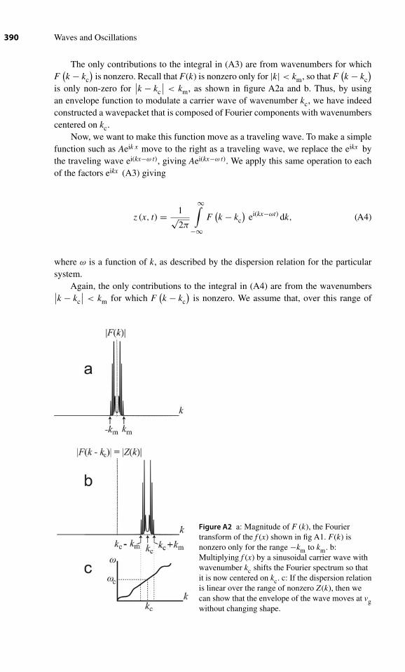
390 Waves and Oscillations
The only contributions to the integral in (A3) are from wavenumbers for whichF(k − kc
)is nonzero. Recall that F(k) is nonzero only for |k| < km, so that F
(k − kc
)is only non-zero for
∣∣k − kc
∣∣ < km, as shown in figure A2a and b. Thus, by usingan envelope function to modulate a carrier wave of wavenumber kc, we have indeedconstructed a wavepacket that is composed of Fourier components with wavenumberscentered on kc.
Now, we want to make this function move as a traveling wave. To make a simplefunction such as Aeik x move to the right as a traveling wave, we replace the eikx bythe traveling wave ei(kx−ω t), giving Aei(kx−ω t). We apply this same operation to eachof the factors eikx (A3) giving
z (x, t) = 1√2π
∞∫−∞
F(k − kc
)ei(kx−ωt) dk, (A4)
where ω is a function of k, as described by the dispersion relation for the particularsystem.
Again, the only contributions to the integral in (A4) are from the wavenumbers∣∣k − kc
∣∣ < km for which F(k − kc
)is nonzero. We assume that, over this range of
Figure A2 a: Magnitude of F (k), the Fouriertransform of the f (x) shown in fig A1. F(k) isnonzero only for the range −km to km. b:Multiplying f (x) by a sinusoidal carrier wave withwavenumber kc shifts the Fourier spectrum so thatit is now centered on kc. c: If the dispersion relationis linear over the range of nonzero Z(k), then wecan show that the envelope of the wave moves at vgwithout changing shape.

Appendix A ■ Group Velocity for an Arbitrary Envelope Function 391
wavenumbers we can write the dispersion relation as
ω = ωc + (k − kc
) dω
dk
∣∣∣∣kc
, (A5)
where ωc = ω(kc
)is the angular frequency corresponding to the wavenumber kc of
the carrier wave. In words, our assumption (A5) says that ω depends linearly on k,though it need not be directly proportional. An example of such a dispersion relationis shown in figure A2c. (In fact, if km is small enough, then any dispersion relationwill satisfy this restriction, since any function is linear over a small enough range.)
Defining vg = dω
dk
∣∣∣∣kc
, we can rewrite equation (A5) as
ω = ωc + (k − kc
)vg. (A6)
Substituting this into equation (A4) gives us
z (x, t) = 1√2π
∞∫−∞
F(k − kc
)ei kxe−iωcte−i kvgteikcvgtdk.
Now, we define k′′ ≡ k − kc ⇔ k = k′′ + kc, so that
z (x, t) = 1√2π
∞∫−∞
F(k′′) ei (k′′+kc)xe−iωcte−i (k′′+kc)vgteikcvgtdk.
= 1√2π
∞∫−∞
F(k′′) ei (kcx−ωct)eik′′(x−vgt)dk′′.
Again, k′′ is just a variable of integration, so we can rewrite it as k:
z (x, t) = 1√2π
∞∫−∞
F (k) ei (kcx−ωct)eik(x−vgt)dk ⇒
z (x, t) = ei (kcx−ωct) 1√2π
∞∫−∞
F (k) eik(x−vgt)dk. (A7)
Since equation (A1): f (x) = 1√2π
∞∫−∞
F (k) eikxdk, we have that
f(
x − vgt)
= 1√2π
∞∫−∞
F (k) eik(x−vgt)dk,
so that equation (A7) becomes
z (x, t) = ei (kcx−ωct) f(
x − vgt)
.
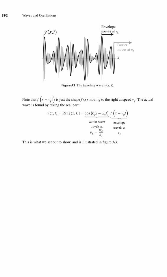
392 Waves and Oscillations
Figure A3 The traveling wave y (x, t).
Note that f(
x − vgt)
is just the shape f (x) moving to the right at speed vg. The actual
wave is found by taking the real part:
y (x, t) = Re [z (x, t)] = cos(kcx − ωct
)︸ ︷︷ ︸carrier wave
travels at
vp = ωc
kc
f(
x − vgt)
︸ ︷︷ ︸envelope
travels at
vg
This is what we set out to show, and is illustrated in figure A3.

Index
AC circuits 18adiabatic compression 310adiabatic index 311adjoint 154adjustable constants 7AFM 93, 130aliasing 275AM radio 32, 106, 121, 329, 341Ampère’s Law 287amplitude 5amplitude, resonance 89–92analogy: normal mode analysis & vector
analysis 160analogy: particle in a box & string 243analogy: quantum bound states & standing
waves on string 280analogy: rope waves & quantum waves 344analysis, general, with orthonormal basis 250Angstrom 59angular frequency 6Annual Percentage Rate 78antinode 314anti-reflection coating 384APR 78arctangent 8atomic energy levels 164Atomic Force Microscopy (AFM) 93, 130attractor 122, 125average value of squared sinusoid 97Avogadro’s number 310
bank interest 78basin of attraction 123basis 156basis functions 248beaded string 216beaded string, driven 238
beaded string, eigenvector 227beaded string, normal mode analysis 226beats 137Boltzmann’s Constant 310bonding orbital 164bound charge 298bound current 298boundary condition 220–221boundary conditions 345bra 155bra-ket notation 155breathing mode 142bulk modulus 311butterfly effect 123
c 290cantilever 52–56cantilever, effective mass of 56cantilever, spring constant of 55capacitance per unit length 303capacitor 10capacitor, impedance of 19capillary waves 341carbon nanotube 57carrier wave 121, 328, 330, 331, 388–390Cartesian representation 15Casimir effect 28causality 368Cavendish experiment 52Cavendish, Henry 51chaos 123characteristic equation 186–187characteristic impedance 360, 363, 382characteristic length 75charge 10circular polarization 336clarinet 316
393

394 Index
CO2 molecule 214coaxial cable 301cocoa 338commuting operations 17, 181complete basis 159complex conjugate 15complex exponential 13complex plane 14complex version of current 19complex version of voltage 19Continuity Equation 307continuous functions, inner
product of 232continuous string 230contrast for MRI 111cosine, Taylor series for 13coupled DEQs 141coupled oscillators, driven 166coupled pendula 139critically damped behavior 73crystals, waves in 226current 10current, complex version of 19
damped electrical oscillator 68damping 64damping constant 64dB 322DCT 267decibels 322degenerate modes 206del 337delocalized particle 24delta function, Dirac 272delta function, Kronecker 197denegeracy 206DEQ 4DEQ, linear 7DEQs, coupled 141derivative, partial 281determinant 181–182DFT 263DFT, frequency resolution 259DFT, maximum frequency for 260DFT, order of frequencies 263–264diamagnetic 298dielectric 297dielectric constant 297difference frequency 121
differential equation 4dipole 297Dirac delta function 272Dirac notation 155Discrete Cosine Transform 267Discrete Fourier Transform (see DFT) 263dispersion relation 221, 323displacement in a sound wave 305diving board 52–56DNA 377dog pulling a spring 43dot notation 5double pendulum 213drag coefficient 76drag force 64driven beaded string 238driven coupled oscillators 166driven oscillator in complex plane 89driven oscillator, energy of 95–99driven oscillator, full solution for 103driving force, sinusoidal 86dynamical variables 124
earthquakes 48eddy currents 77effective mass of a cantilever 56effective spring constant 40eigenfunctions for string 233eigenstates 152eigenvalue 186eigenvalue equation 186eigenvalues for two coupled oscillators 188eigenvector 157, 186eigenvector for beaded string 227elastic limit 45electrical oscillator 10electrical oscillator, damped 68electrical resonance 104electromagnetic waves 289, 290, 292electron volt 173electron, group velocity of 331em waves 289, 290, 292energy density of B 317energy density of E 317energy density of em radiation 318energy of a superposition state 151energy of driven oscillator 95–99energy, exponential decay of 69energy, potential, of an oscillator 17

Index 395
energy, total, of an oscillator 17energy-time uncertainty principle 28envelope function 66equation of motion 5equilibrium 3equilibrium length 8, 44equipartition theorem 80Euler, Leonhard 14Euler’s equation 13Euler’s equation for fluids 309eV 173evanescent wave 373, 376, 377evaporation, thermal 49expectation value 152, 277exponential decay of energy 69exponential, complex 13
Faraday’s Law 10, 78, 287Fast Fourier Transform 265FFT 265fiber optics 324, 328, 329, 371, 373filter, low pass 21, 37first harmonic 314first-order approximation 12flute 102, 314flux, magnetic 10, 78FM radio 32, 121FMAFM 130force from the left 294Fourier analysis 252–254, 269Fourier analysis, complex
exponential 254, 269Fourier analysis, wavenumber 248Fourier expansion 252–254, 269Fourier transform 255, 269Fourier, Joseph 246fractal 123, 128free charge 297free electron 24free electron dispersion relation 325frequency 6frequency modulation AFM 130frequency resolution 259frequency, highest possible 223frequency-time uncertainty relation 27fret 240full solution for driven oscillator 103Full Width at Half Maximum 98–99, 256functions for rope waves 344
functions, inner product of 232fundamental 314FWHM 98–99, 256
Galileo 40gas pressure sensor 71–72Gauss’s Law 287Gaussian function 255general solution 7, 103gravity waves 341ground plane 301ground, electrical 18group velocity 327, 329, 330, 388group velocity derivation 388group velocity of electron 331guitar 239–240gyromagnetic ratio 107–108gyroscope 108
Hanning window 259harmonic approximation 3harmonic generation 114, 119harmonics on a guitar 240Heisenberg uncertainty principle 29, 277helium, supersolid 61helix 125Hermitian conjugate 154Hermitian matrix 199Hermitian transpose 154heterodyning 121H-field 298hi 327highest possible frequency 223highest possible wavenumber 225high-pass filter 36Hilbert space 153Hilbert space, rescaling for unequal
masses 208Hilbert, David 159homogeneous differential equation 7, 102Hooke, Robert 4Hooke’s Law 4hot cocoa 338hydrostatic pressure 311
ideal gas law 310identity matrix 198

396 Index
IDFT 263impedance 19impedance matching 383impedance of capacitor 19impedance of inductor 23impedance of linear materials 366impedance, characteristic 360, 363, 382impedance, mechanical 354–355index of refraction 366inductance per unit length 303inductor 10inductor, impedance of 23initial position 7initial velocity 7inner product 154inner product of functions 232instrument, reed 316instruments, musical 314intensity 318intensity of em waves 300interest, bank 78Inverse Discrete Fourier Transform 263inverse matrix 198, 211ionosphere 31, 341isomorphism 11isomorphism: em waves in linear
materials & in vacuum 300isomorphism: em waves in vacuum & rope
waves 296, 336isomorphism: longitudinal & transverse
waves 228isomorphism: mechanical & electrical
oscillators 105isomorphism: sound & em waves 313, 340isomorphism: transmission line waves &
em waves in vacuum 304, 339isomorphisms, key equations for 293isomorphisms, summary of 368isothermal compression 312
jpeg image compression 266
ket 155key equations for isomorphisms 293keyboard 170Kirchoff’s Loop Rule 11Kronecker delta function 197k-space 234–235
laminar flow 64Laplacian 337Larmor frequency 110laser tweezers 82LC oscillator 10Lennard-Jones potential 59lens 370lensmakers equation 371light 291light, speed of 290linear DEQ 7linear materials 297linear materials, impedance of 366linear materials, Maxwell’s equations in 299local oscillator 121longitudinal oscillations 227low-pass filter 21, 37lumped circuit element model 302
magnetic flux 10, 78magnetic moment 107magnetic pendulum 122Magnetic Resonance Imaging 85, 107magnetic susceptibility 298magnetization 110magnitude of a complex number 15mass matrix 201material parameters table 46matrix multiplication 179–180maximum frequency for DFT 260maximum wiggliness 225Maxwell’s equations 287Maxwell’s equations in linear materials 299mechanical impedance 354–355MEMS 42, 62microphone 327mixing 120mnemonic for phase upon reflection 366mode index 195molecular energy levels 164molecular orbitals 164moment of inertia 41momentum wave 293momentum, quantum mechanical 28momentum, transverse 293MRI 85, 107musical instruments 314musical scales 170
Index 397
Nano ElectroMechanical Systems 56nanotube, carbon 57negative frequencies 257NEMS 56Newton, Isaac 4NMR 107node 220nonlinear dispersion 324non-linear oscillators 114non-normalized basis functions 250normal mode analysis 149, 195normal mode analysis for beaded
string 226normal mode coordinates 143, 144, 201normal mode expansion 161normal modes 142, 149normalized vector 157normalizing eigenvectors 194Nuclear Magnetic Resonance 107
Ohm’s Law 19operator 180optic axis 370organ pipes 316orthogonal 158orthogonality of eigenvectors 205–207orthonormal basis 159orthonormal basis, general analysis with 250orthonormality, equivalent of for unequal
masses 207oscillation, harmonic, requirements for 39oscillator, driven, energy of 95–99oscillator, driven, full solution for 103oscillator, driven, in complex plane 89oscillator, electrical 10overdamped behavior 72
Pa 45panic, let’s not 326parallel axis theorem 42parallel impedance 21parallel RLC oscillator 136paramagnetic 298parameter 7Parseval’s theorem 275partial derivative 281particle in a box 243particular solution 103
Pascal 45p-brane 216peak frequency 91pendulum 40pendulum force 42pendulum mode 142pendulum, simple 41period 6period doubling 126permeability 298permittivity 297personality archetypes 151phase 6phase factor for driven oscillator 88, 89phase space 124phase upon reflection, mnemonic
for 366phase velocity 284, 323phonon 325photon 113piezoelectric 49Planck’s constant 28plane wave 288, 292plano-convex lens 370plasma 31plasma frequency 32Poincaré section 125polar representation 15polarization 297, 374polarization, circular 336potential energy of an oscillator 17power carried by waves 317power for driven oscillator 98power in transmission line waves 339power resonance curve 98Poynting vector 291, 300, 319precession 108pressure 305pressure broadening 114prism 385probability density 24proton 107pure sinusoid 26
Q 70, 92QCM 47, 49quality factor 70, 92quantization of energies 221quantization of frequencies 221

398 Index
quantum beats 171quantum superpositions 151Quartz Crystal Microbalance 47, 49quietest sound 322
radiation damping 81radio 32, 106, 121, 329, 341radio frequency 110radio receiver 105–106radio, AM 32, 106, 121, 329, 341radio, FM 32, 121radioactive particles 58ray 368RC filter 21, 36, 37real space 235reed instrument 316reflected wave 344, 347, 358–359reflection 375refraction 369rescaling Hilbert space for unequal
masses 208resistor 19resonance 84resonance amplitude 89–92resonance curve, power 98Reynolds number 75Reynolds, Osborne 75RF 110RFID tags 383RG58 cable 304, 362rigid shape moving 283RL filter 23, 37RLC oscillator 105, 136rms amplitude 319room mean square amplitude 319rope waves, functions for 344rotating reference frame 110rotation matrix 210, 211rotor 51rubber band 240
sampling 258scales, musical 170Schrödinger’s equation 285Sears Tower 58second-order approximation 12second-order DEQ 4self-adjoint 200
self-sustaining oscillation 291semiclassical description 107sensitivity to initial conditions 121sensor, gas pressure 71–72series impedance 21shear 47shear modulus 48shear modulus table 46Shear, William 48SHM 6signal generator 18simple harmonic motion 6simple harmonic motion, in complex
plane 16, 18simple pendulum 41sine, Taylor series for 13sinusoid, pure 26slippery devil 8smallest possible wavelength 225Snell’s Law 369, 375solution for a DEQ 4sonogram 265sound intensity 321sound waves 305sound, speed of (see speed of sound) 311spectroscopy 113speed of light 290speed of sound 310speed of sound in a gas 311speed of sound in liquid 312speed of sound in solid 312spherical aberration 370spin angular momentum 107spin down 112, 164spin up 112, 164spring 9spring constant 4spring cut in half 43spring, vertical 9square wave 134, 252squared sinusoid, average value of 97stable equilibrium 3standard deviation 278standing waves 219steady state behavior 87Stokes, George 74Stokes’ Law 74strain 45strain hardening 45

Index 399
strange attractor 128stress 45string, beaded, driven 238string, eigenfunctions 233string, frequencies for 230string, normal mode analysis 234sub-harmonic resonance 119superposing normal modes 146Superposition Principle for driven
systems 101Superposition Principle for traveling
waves 285supersolid 61surface tension 341susceptibility 298
Taipei 101 60tapping mode AFM 93Taylor series 12Taylor series, three important
uses of 34television 33terminator 343, 362thermal evaporation 49thermal vibrations 80thickness monitor 49thin film interference 384three-dimensional waves 337three-step procedure 4tilde 19TIRFM 377top, child’s 108torque due to magnetic field 108torsion balance 52torsional oscillator 51total energy of an oscillator 17total internal reflection 371transients 102transmission line waves, power in 339transmission line, impedance
of 360, 363, 382transmission lines 301transmitted wave 344, 350, 358–359transverse momentum 293traveling wave 283traveling wave speed 284triangle wave 270trumpet 316tube, torsion of 50–51
turbulent flow 64two-slit experiment 271
ultimate stress 45uncertainty 26underdamped behavior 72Universal Gas Constant 310
Van der Waals attraction 59viscosities, table of 75viscosity 74viscous damping 64voltage 10voltage, complex version of 19
washing machine 86watch crystal 70–71water waves 341wave equation 282wave equation, solutions 283wave function, real and imaginary
parts 25wavefront 368wavefunction 24wavenumber 24, 220wavenumber for Fourier analysis 248wavepacket 326waves in crystals 226wavevector 337weasel 135, 382well-tempered scale 170whale call 266wind instruments 314wind tunnel 64windowing 259, 276wire, torsion of 61
yield stress 45yield stress table 46yielding 45Young, Thomas 44, 271Young’s modulus 44Young’s modulus table 46
zeroth-order approximation 12