wavex: extracting wavelets from seismic data - … · the mathematica® journal wavex: extracting...

The Mathematica® Journal

WaveX: Extracting Wavelets from Seismic DataJohn M. NovakMathematica is a powerful tool for the analysis and manipulation of data. Itcan be used to provide a competitive edge in many commercial endeavors,including the field of petroleum exploration. One of the many tools cre-ated in Mathematica by GMG/AXIS for internal use is WaveX, a tool forextracting relative wavelets from seismic data based on well log informa-tion. Here we demonstrate some of the uses of the tool and discuss howMathematica allowed us to create a superior tool.

‡ The ProblemPetroleum exploration employs a variety of methods for characterizing theearth! s subsurface while seeking potential hydrocarbon reservoirs. One of themost common techniques used on land is to create vibrations on the surface,perhaps by a dynamite explosion, then to listen via an array of geophones forechoes from beneath the surface. This and associated technologies are collec-tively called seismic exploration.

The seismic data recorded by the sensors around the explosion are processed andmassaged to extract meaningful signals, which may be visualized as an image ofthe subsurface. These images can then be analyzed with the goal of understand-ing something about the structure of the earth, such as the types and nature ofthe rock and whether fluids, such as oil or gas, exist within pores in the rock.

One way to calibrate the seismic data gathered at the surface with the propertiesof the earth is to drill a hole, or well, into the earth. We can more directlymeasure the characteristics of the earth at that point. This information can thenbe compared to the seismic data, a process called a well tie. Tying the wellinvolves matching correlative events observed in the well (or the well log, typicallyacoustic velocity and bulk density measurements) with the seismic data. Thisprocess generates a waveform whose features can be used to assess and adjust theseismic data. This waveform is called a wavelet. (The wavelet is not the same asthe mathematical structure of the same name.) The character of the extractedwavelet can also provide feedback about the quality of the well tie.

Commercial software used for tying wells and extracting wavelets imposescertain algorithms and methodologies upon the user. GMG/AXIS Geophysicsdesired a more flexible tool that could be modified to suit the peculiarities ofindividual data sets and could be adapted to different algorithms. Mathematicaappeared to be an effective platform on which to create this tool.

The Mathematica Journal 9:3 © 2005 Wolfram Media, Inc.

Commercial software used for tying wells and extracting wavelets imposescertain algorithms and methodologies upon the user. GMG/AXIS Geophysicsdesired a more flexible tool that could be modified to suit the peculiarities ofindividual data sets and could be adapted to different algorithms. Mathematicaappeared to be an effective platform on which to create this tool.

‡ The SolutionWith the creation of a number of functions for seismic file import, graphicsdisplay, and data analysis, Mathematica was converted into a powerful environ-ment for well ties and wavelet extraction. The following sequence of inputsdemonstrates an example workflow using this functionality in Mathematica 5.

The flow begins by loading the packages with the required utility. On produc-tion machines, this is typically autoloaded.

<< Seismic‘

Next, we load in the data, consisting of the well log to be tied and a window ofseismic data from receivers near the well location. In this case, we specify one setof data, or trace, from each side of the well location, forming a 3 µ 3 grid oftraces. The data set can then be manipulated by a handle, which we return andhere store in the variable dset.

dset = LoadWaveXData@"welllog.las", "seismic.segy", 1DColumns:8DEPTH, CALI, DT, EGRCN, ERHOB, ILD, COND, TDPAIR_DT, DT_CLEAN,

GR_MEDIAN, GR_DT, GR, USEDPOR, QL_VSH, DT_NODEPTH, SONIC_ROTATION,DT_ND_EDIT, DT_EDIT, DT_ND_CORRECTED, COAL, DT_EDIT_BACKUP,DT_EDIT_DRIFT, DT_EDIT_COPY, DT_EDIT_CORRECTED, DT_SEISMIC<

run1

Separating out the correlation stage from the data loading allows us to iteratecorrelations without the expense of reloading the data.

The well log data typically consists of a series of measurements of rock velocityand density at half-foot increments. Seismic data is measured in time, while thelog data is in depth; these must be put in the same domain for further compari-son. By finding the rock velocities within the well, we can estimate the traveltime for a shock wave going from the surface, down to a particular depth, andback up to the receiver. This data is usually not complete, however, which maycause us to incorrectly estimate a travel time corresponding to depth. Well logdata can also suffer from systematic errors in measurement, which can beaccounted for when tying the log by applying a small time shift between the welllog (sonic) and the seismic data. The user does this by specifying the correspon-dence between particular times in the two data sets. The sonic can also bestretched out in time to compensate for other systematic effects; this is given as arange of percentage stretches. A portion of the seismic and the sonic are thencorrelated over some range of lags, given below as 900 milliseconds of datacorrelated over ±200 milliseconds.

556 John M. Novak


283-488283-488

283-489283-489

283-490283-490

284-488284-488

284-489284-489

284-490284-490

285-488285-488

285-489285-489

285-490285-490

283-488283-488

283-489283-489

283-490283-490

284-488284-488

284-489284-489

284-490284-490

285-488285-488

285-489285-489

285-490285-490

200. 200.

150. 150.

100. 100.

50. 50.

0 00 0

-50. -50.

-100. -100.

-150. -150.

-200. -200.

0.182

0.305

0.243

-1.0% 1.0%

The well log data typically consists of a series of measurements of rock velocityand density at half-foot increments. Seismic data is measured in time, while thelog data is in depth; these must be put in the same domain for further compari-son. By finding the rock velocities within the well, we can estimate the traveltime for a shock wave going from the surface, down to a particular depth, andback up to the receiver. This data is usually not complete, however, which maycause us to incorrectly estimate a travel time corresponding to depth. Well logdata can also suffer from systematic errors in measurement, which can beaccounted for when tying the log by applying a small time shift between the welllog (sonic) and the seismic data. The user does this by specifying the correspon-dence between particular times in the two data sets. The sonic can also bestretched out in time to compensate for other systematic effects; this is given as arange of percentage stretches. A portion of the seismic and the sonic are thencorrelated over some range of lags, given below as 900 milliseconds of datacorrelated over ±200 milliseconds.

WaveXCorrelate@dset, StretchRange Ø 8-1, 1, 2<,SonicTie Ø 950, TieLength Ø 900, CorrelationLength Ø 200D;

So, each extracted seismic trace is cross-correlated with each stretched sonic log.For the parameters used previously, this results in 18 time series of ±200 millisec-onds in length. We are interested in knowing the value and location of the peakcorrelation coefficients. The function ShowCorrelations displays all the correla-tions, instantaneous amplitude envelopes, pointers to the peak locations, and soon. The bar on the left gives the color coding for the correlation pointers; thisexample underlays the data with a density plot of the amplitudes, which in somecases may make some features more obvious.

ShowCorrelations@dset, ColorFunction Ø GrayScaleD

Examining the previous graph, we may decide that 1% stretch provides the bestcorrelations. We select it for further operations.

PickStretch@dset, 1.0Drun2

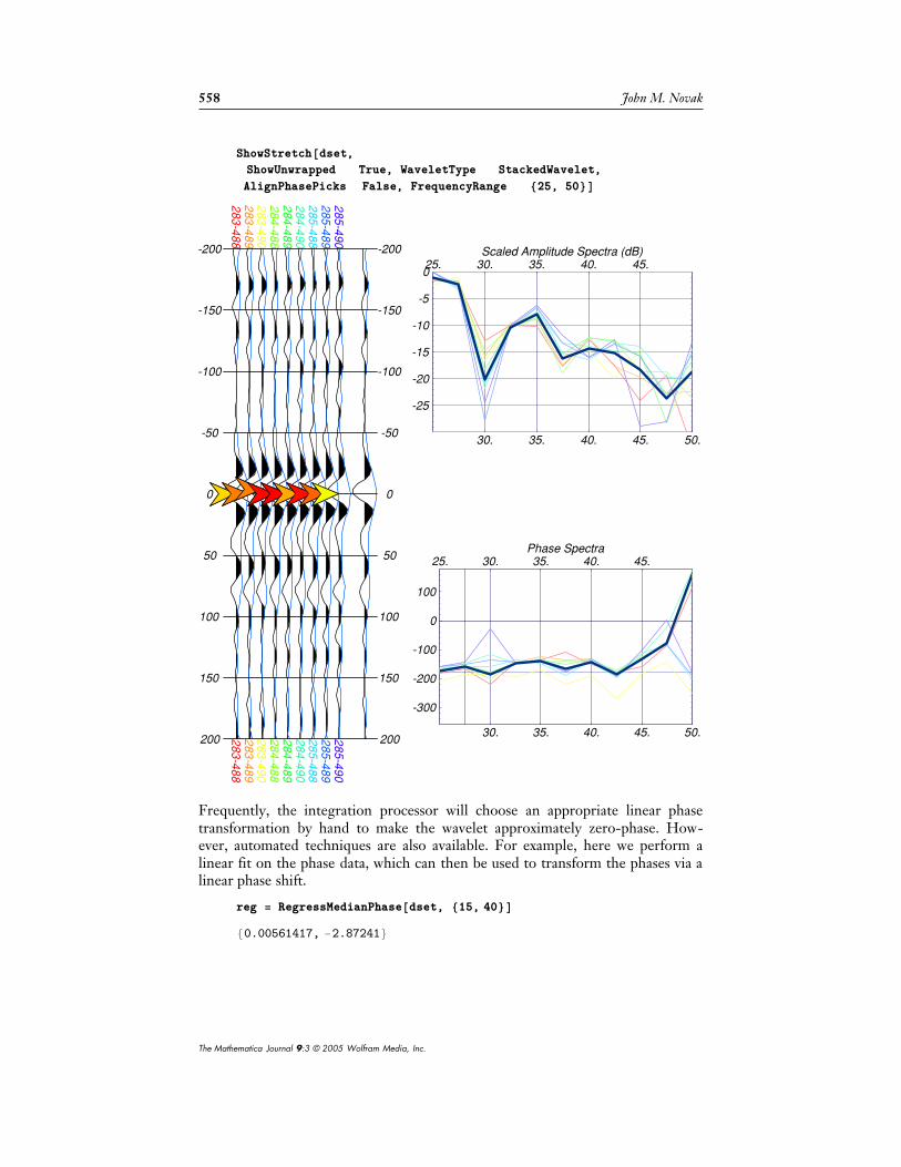
The correlations are combined to give us a prototype for the wavelet. They maybe combined in different ways, the simplest being a stack, or average. The idealseismic wavelet in this context is zero-phase; for our purposes this means wewant the phase spectra over the dominant frequency range to be near zero.ShowStretch can be used to display the characteristics of the correlations andthe extracted wavelet (where the wavelet is the rightmost vertical trace in thefollowing graphic).

WaveX: Extracting Wavelets from Seismic Data 557


283-488283-488

283-489283-489

283-490283-490

284-488284-488

284-489284-489

284-490284-490

285-488285-488

285-489285-489

285-490285-490

-200 -200

-150 -150

-100 -100

-50 -50

0 0

50 50

100 100

150 150

200 200

30. 35. 40. 45. 50.

-25

-20

-15

-10

-5

025. 30. 35. 40. 45.

Scaled Amplitude Spectra (dB)

30. 35. 40. 45. 50.

-300

-200

-100

0

100

25. 30. 35. 40. 45.Phase Spectra

ShowStretch@dset,ShowUnwrapped Ø True, WaveletType Ø StackedWavelet,AlignPhasePicks Ø False, FrequencyRange Ø 825, 50<D

Frequently, the integration processor will choose an appropriate linear phasetransformation by hand to make the wavelet approximately zero-phase. How-ever, automated techniques are also available. For example, here we perform alinear fit on the phase data, which can then be used to transform the phases via alinear phase shift.

reg = RegressMedianPhase@dset, 815, 40<D80.00561417, -2.87241<

558 John M. Novak


LinearPhaseShift@dset, regDrun2

We can view the transformed wavelet, which now looks much closer to thedesired shape with a strong central peak and balanced side lobes.

ShowStretch@dset, WaveletType Ø StackedWavelet,AlignPhasePicks Ø False, FrequencyRange Ø 825, 50<D

This extracted wavelet and the well logs can then be used to generate a syntheticseismic trace, which can be compared to the actual seismic data to verify thequality of the tie. If the tie is good, we would expect events (significant peaks andtroughs in the time series) to be aligned between the synthetic and the realseismic. The synthetic data is generated by assuming that a sufficiently largevelocity or density contrast in the rock will correspond to a reflection; thus, fromthe well logs, we can generate a time series of reflection coefficients that, whenconvolved with a wavelet, should look much like the seismic data.



283-488283-488

283-489283-489

283-490283-490

284-488284-488

284-489284-489

284-490284-490

285-488285-488

285-489285-489

285-490285-490

-200 -200

-150 -150

-100 -100

-50 -50

0 0

50 50

100 100

150 150

200 200

30. 35. 40. 45. 50.

-25

-20

-15

-10

-5

025. 30. 35. 40. 45.

Scaled Amplitude Spectra (dB)

30. 35. 40. 45. 50.

-150

-100

-50

0

50

100

150

25. 30. 35. 40. 45.Phase Spectra

This extracted wavelet and the well logs can then be used to generate a syntheticseismic trace, which can be compared to the actual seismic data to verify thequality of the tie. If the tie is good, we would expect events (significant peaks andtroughs in the time series) to be aligned between the synthetic and the realseismic. The synthetic data is generated by assuming that a sufficiently largevelocity or density contrast in the rock will correspond to a reflection; thus, fromthe well logs, we can generate a time series of reflection coefficients that, whenconvolved with a wavelet, should look much like the seismic data.

Seismic data is frequently collected from a single line of sensors, in which casethe data is called 2D, or from a grid of sensors, where it is known as 3D. In thiscase, the data is 3D, but for conciseness we will only compare the synthetic to asingle line of receivers via the Show3DØFalse option. Furthermore, as indicatedpreviously, the start of the well data is often questionable, so we frequently createan artificial well log for this starting section, which can be adjusted for thealignment we derived. Here we suggest to the routines that the first 800 feet ofdata can be replaced by an artificial curve.

ShowSynthetic@dset, VelocitiesCutoff Ø 800, Show3D Ø FalseDms0

200

400

600

800

1000

1200

1400

1600

1800

2000

ft0

1000

2000

3000

4000

5000

6000

7000

8000

9000

10000

11000

12000

140 40

Slownessms0

200

400

600

800

1000

1200

1400

1600

1800

2000

560 John M. Novak


ms0

200

400

600

800

1000

1200

1400

1600

1800

2000

ft0

1000

2000

3000

4000

5000

6000

7000

8000

9000

10000

11000

12000

140 40

Slownessms0

200

400

600

800

1000

1200

1400

1600

1800

2000

Once we are satisfied with the results, the extracted wavelet, synthetic seismic,and modified logs can be saved for handling elsewhere.

Naturally, the previous flow demonstrates only a few of the many options avail-able to a user; many of these functions include numerous options to control thenature of the display or the format of the data. A large selection of transforma-tions to perform on the data are also present, and Mathematica’s programmingenvironment allows arbitrary additional manipulations as required.

‡ Detailed IssuesHere are a few of the many particular design issues encountered in creating thetool suite, which may be of special interest to programmers.

· Data StructuresOne feature that an experienced Mathematica user will immediately notice is theuse of a handle to the data (a string name), instead of the more familiar func-tional manipulation of lists of data. There are several reasons for this unusualdesign choice, the most important of which is that seismic data sets can be verylarge. If the data lists were returned directly by load routines and the user forgotto suppress the output, it is likely that the machine would hang for significantamounts of time as the front end attempts to format the output data. For WaveXmanipulations, this might be tens of thousands of data points; for other manipula-tions of seismic data, this could easily be hundreds of thousands of data points onthe low end. (Data sets of hundreds of gigabytes are not uncommon, thoughthese are not read all at once into Mathematica.) The use of handles in this toolsetis an attempt to shield the user from this effect.



One feature that an experienced Mathematica user will immediately notice is theuse of a handle to the data (a string name), instead of the more familiar func-tional manipulation of lists of data. There are several reasons for this unusualdesign choice, the most important of which is that seismic data sets can be verylarge. If the data lists were returned directly by load routines and the user forgotto suppress the output, it is likely that the machine would hang for significantamounts of time as the front end attempts to format the output data. For WaveXmanipulations, this might be tens of thousands of data points; for other manipula-tions of seismic data, this could easily be hundreds of thousands of data points onthe low end. (Data sets of hundreds of gigabytes are not uncommon, thoughthese are not read all at once into Mathematica.) The use of handles in this toolsetis an attempt to shield the user from this effect.

The handles also provide a convenient means of grouping associated data,forming a sort of ad-hoc database. For example, a number of functions will placeintermediate results in a symbol of the form name[handle]=data, which can thenbe retrieved for later analysis. Over time, utilities have been evolved for this toolsuite to streamline the process and allow the user to determine what data isavailable after operations. The data can then be easily extracted for input intomore traditional Mathematica functions, though of course the user must then takespecial care to suppress large output.

For a parallel to other functions, consider the use of handles to streams (e.g.,InputStream) or to notebooks (e.g., NotebookObject). While in these cases, thehandle is to data stored in an external program, the basic principle is similar.

· File FormatsThere are a number of file formats for handling both seismic data and well logs.However, two particular formats are most common. The SEG-Y format forseismic data is a binary format, which typically has floating-point values stored ina rarely used IBM floating-point format, a header section using EBCDIC charac-ter encoding, and record headers in a binary integer format. The LAS format forlog data, on the other hand, is an ASCII text format storing data in a simplecolumnar format, but with a series of headers that detail various useful sorts oflog information. Each format provides its own challenges for the implementationof import/export routines.

One immediate design point that had to be considered was whether this function-ality should tie into the standard functions Import and Export. In the end, thisdecision was driven primarily by implementation time constraints, and thesimpler choice of creating separate functions for the import and export of thesedata types was used.

An issue regarding the reading of binary data had to do with efficiency. Seismicdata sets are quite large, so care was first taken to provide mechanisms forextracting only the specified portions of the data. The use of stream manipula-tion capabilities via StreamPosition was quite valuable. Unfortunately, we arestill constrained by 2 gigabyte limits in Mathematica’s file-handling capabilities,but there is optimism that with the increasing availability of 64-bit computing,we will soon be able to deal with larger files.

Because the trace data was stored in a nonstandard format, we could not drawdirectly on the Experimental‘BinaryImport function, or on the Utilities‘BiÖnaryFiles‘ standard package. Instead, a list of bytes was read in via ReadÖList[stream, Byte], which could then be transformed by internal conversionroutines. The functions initially partitioned the list into groups of four bytes,which then were transformed into the corresponding floating-point numbers. Asmall compiled function (generated with Compile) was used for the transforma-tion, which provided some speed improvement. However, it was discovered thatif the flat list of input bytes were provided to a compiled function that processeda whole trace at once, a substantial performance improvement could be seen.The lesson is that compiled functions become more useful if we can move theentire processing loop inside, though unfortunately some sacrifice in modularitymust be made with the current capabilities of Compile.

562 John M. Novak


Because the trace data was stored in a nonstandard format, we could not drawdirectly on the Experimental‘BinaryImport function, or on the Utilities‘BiÖnaryFiles‘ standard package. Instead, a list of bytes was read in via ReadÖList[stream, Byte], which could then be transformed by internal conversionroutines. The functions initially partitioned the list into groups of four bytes,which then were transformed into the corresponding floating-point numbers. Asmall compiled function (generated with Compile) was used for the transforma-tion, which provided some speed improvement. However, it was discovered thatif the flat list of input bytes were provided to a compiled function that processeda whole trace at once, a substantial performance improvement could be seen.The lesson is that compiled functions become more useful if we can move theentire processing loop inside, though unfortunately some sacrifice in modularitymust be made with the current capabilities of Compile.

The SEG-Y and LAS formats were developed by industry organizations, but notall implementors follow the data format guidelines precisely. This meant that theroutines had to be written to account for variations found in practice. This wasparticularly common for the LAS data format, where we encountered a numberof files that were contrary to the design specification. The code had to be suffi-ciently modular to be easily adapted to these variations. Rule-based program-ming proved to be quite valuable in this context.

‡ ConclusionsMathematica’s powerful programming capabilities combined with the notebookinterface proved to be an effective system for performing well ties and extractingthe relative wavelet, among many other geophysically-related tasks. A significantamount of development was required to start operating in the data environment,but once targeted data import, export, and visualization functionality was avail-able, the possibilities were limited only by the researcher’s imagination.

The use of Mathematica has expanded into many areas in our company, includingwell log editing, residual velocity analysis, amplitude-versus-offset analysis, andother specialized uses, as well as report preparation for clients (via HTMLexport) and internal research. Mathematica has once again proven itself to be apowerful environment for technical computation.

About the AuthorJohn M. Novak developed a number of Mathematica’s standard add-on packagesand applications for Wolfram Research, Inc. He now works for the AXIS ImagingDivision of the seismic data processing company GX Technology (a subsidiary ofInput/Output, Inc.), helping to spread the use of Mathematica to new arenas.

John M. NovakGX Technology Corporation225 E. 16th Ave. Suite 1200Denver, CO [email protected]



wavex: extracting wavelets from seismic data - … · the mathematica® journal wavex: extracting...

Documents