appendix a introduction to mathematica...
TRANSCRIPT
Appendix A
Introduction toMathematicaCommands
c© Copyright 2004 by Jenny A. Baglivo. All Rights Reserved.
Mathematica (Wolfram Research, Inc.) is a system for doing mathematics onthe computer and for reporting the results. Mathematica has numerical, graphical,and symbolic capabilities. Its basic features include arbitrary precision arithmetic;differential and integral calculus (routines for both symbolic and numerical eval-uation); infinite and finite series, limits and products; expansion and factoring ofalgebraic expressions; linear algebra; solving systems of equations; and two- andthree-dimensional graphics. Mathematica packages and custom tools include pro-cedures for probability and statistics.
This chapter briefly describes the Mathematica commands used in the labo-ratory problems. The first section covers commands provided by the system, andcommands loaded from Mathematica packages. The second section covers the cus-tomized tools provided with this book. An index to the commands appears at theend of the chapter.
A.1 Standard commands
This section introduces the standard Mathematica commands used in the laboratoryproblems. Standard commands include commands provided by the system and com-mands loaded from add-on packages when the StatTools packages are initialized.Note that commands from the
Graphics‘FilledPlot‘,Statistics‘DataManipulation‘,Statistics‘DescriptiveStatistics‘,Statistics‘DiscreteDistributions‘, andStatistics‘ContinuousDistributions‘
packages are loaded when StatTools‘Group1‘ and StatTools‘Group2‘ are initial-ized, commands from
Statistics‘ConfidenceIntervals‘ and
1
2 Appendix A. Introduction to Mathematica Commands
Statistics‘HypothesisTests‘
are loaded when StatTools‘Group3‘ is initialized, and commands from
Statistics‘LinearRegression‘
are loaded when StatTools‘Group4‘ is initialized.Online help for each Symbol discussed in this section is available by evaluating
?Symbol. Additional help and examples are available in the Help Browser.
A.1.1 Built-in constants and functions
Frequently used constants and arithmetic functions, functions for sums and prod-ucts, functions from calculus, functions used in counting problems, the numericalapproximation function (N), boolean functions, logical operators and connectors,and a function for producing random integer and random real numbers are summa-rized below.
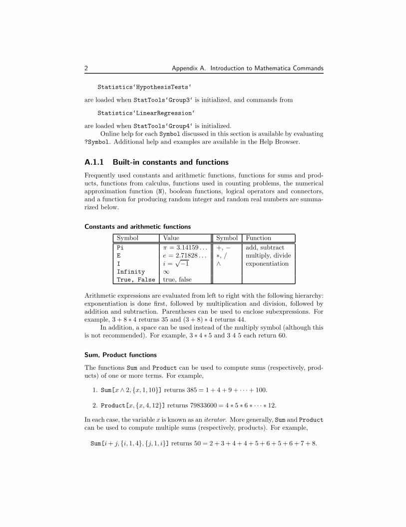
Constants and arithmetic functions
Symbol Value Symbol Function
Pi π = 3.14159 . . . +, − add, subtractE e = 2.71828 . . . ∗, / multiply, divideI i =
√−1 ∧ exponentiation
Infinity ∞True, False true, false
Arithmetic expressions are evaluated from left to right with the following hierarchy:exponentiation is done first, followed by multiplication and division, followed byaddition and subtraction. Parentheses can be used to enclose subexpressions. Forexample, 3 + 8 ∗ 4 returns 35 and (3 + 8) ∗ 4 returns 44.
In addition, a space can be used instead of the multiply symbol (although thisis not recommended). For example, 3 ∗ 4 ∗ 5 and 3 4 5 each return 60.
Sum, Product functions
The functions Sum and Product can be used to compute sums (respectively, prod-ucts) of one or more terms. For example,
1. Sum[x ∧ 2, {x, 1, 10}] returns 385 = 1 + 4 + 9 + · · · + 100.
2. Product[x, {x, 4, 12}] returns 79833600 = 4 ∗ 5 ∗ 6 ∗ · · · ∗ 12.
In each case, the variable x is known as an iterator. More generally, Sum and Product
can be used to compute multiple sums (respectively, products). For example,
Sum[i + j, {i, 1, 4}, {j, 1, i}] returns 50 = 2 + 3 + 4 + 4 + 5 + 6 + 5 + 6 + 7 + 8.
A.1. Standard commands 3
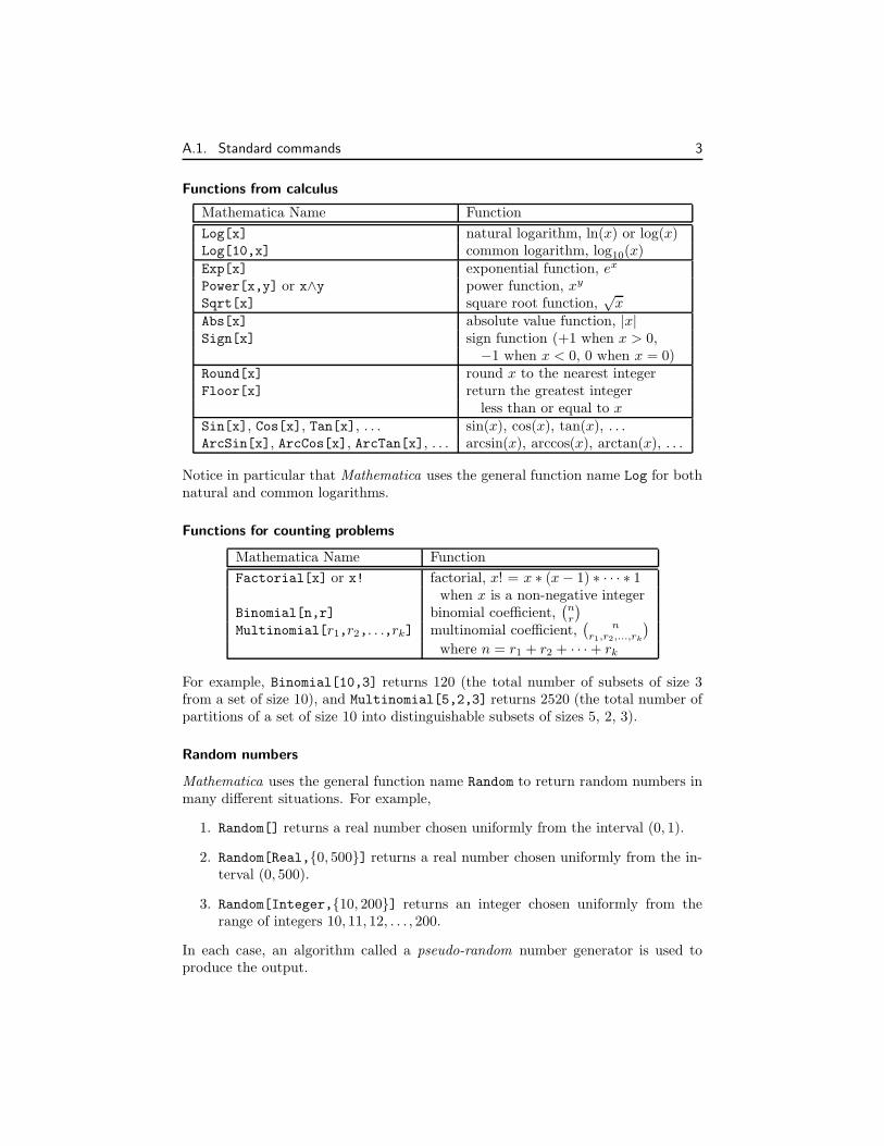
Functions from calculus
Mathematica Name Function
Log[x] natural logarithm, ln(x) or log(x)Log[10,x] common logarithm, log10(x)Exp[x] exponential function, ex
Power[x,y] or x∧y power function, xy
Sqrt[x] square root function,√
xAbs[x] absolute value function, |x|Sign[x] sign function (+1 when x > 0,
−1 when x < 0, 0 when x = 0)Round[x] round x to the nearest integerFloor[x] return the greatest integer
less than or equal to xSin[x], Cos[x], Tan[x], . . . sin(x), cos(x), tan(x), . . .ArcSin[x], ArcCos[x], ArcTan[x], . . . arcsin(x), arccos(x), arctan(x), . . .
Notice in particular that Mathematica uses the general function name Log for bothnatural and common logarithms.
Functions for counting problems
Mathematica Name Function
Factorial[x] or x! factorial, x! = x ∗ (x − 1) ∗ · · · ∗ 1when x is a non-negative integer
Binomial[n,r] binomial coefficient,(nr
)
Multinomial[r1,r2,. . .,rk] multinomial coefficient,(
nr1,r2,...,rk
)
where n = r1 + r2 + · · · + rk
For example, Binomial[10,3] returns 120 (the total number of subsets of size 3from a set of size 10), and Multinomial[5,2,3] returns 2520 (the total number ofpartitions of a set of size 10 into distinguishable subsets of sizes 5, 2, 3).
Random numbers
Mathematica uses the general function name Random to return random numbers inmany different situations. For example,
1. Random[] returns a real number chosen uniformly from the interval (0, 1).
2. Random[Real,{0, 500}] returns a real number chosen uniformly from the in-terval (0, 500).
3. Random[Integer,{10, 200}] returns an integer chosen uniformly from therange of integers 10, 11, 12, . . . , 200.
In each case, an algorithm called a pseudo-random number generator is used toproduce the output.
4 Appendix A. Introduction to Mathematica Commands
Numerical approximation
Mathematica returns exact answers whenever possible. The N function can beused to compute approximate (decimal) values instead. For example, N[E] returns2.71828 and N[40!] returns 8.15915 1047.
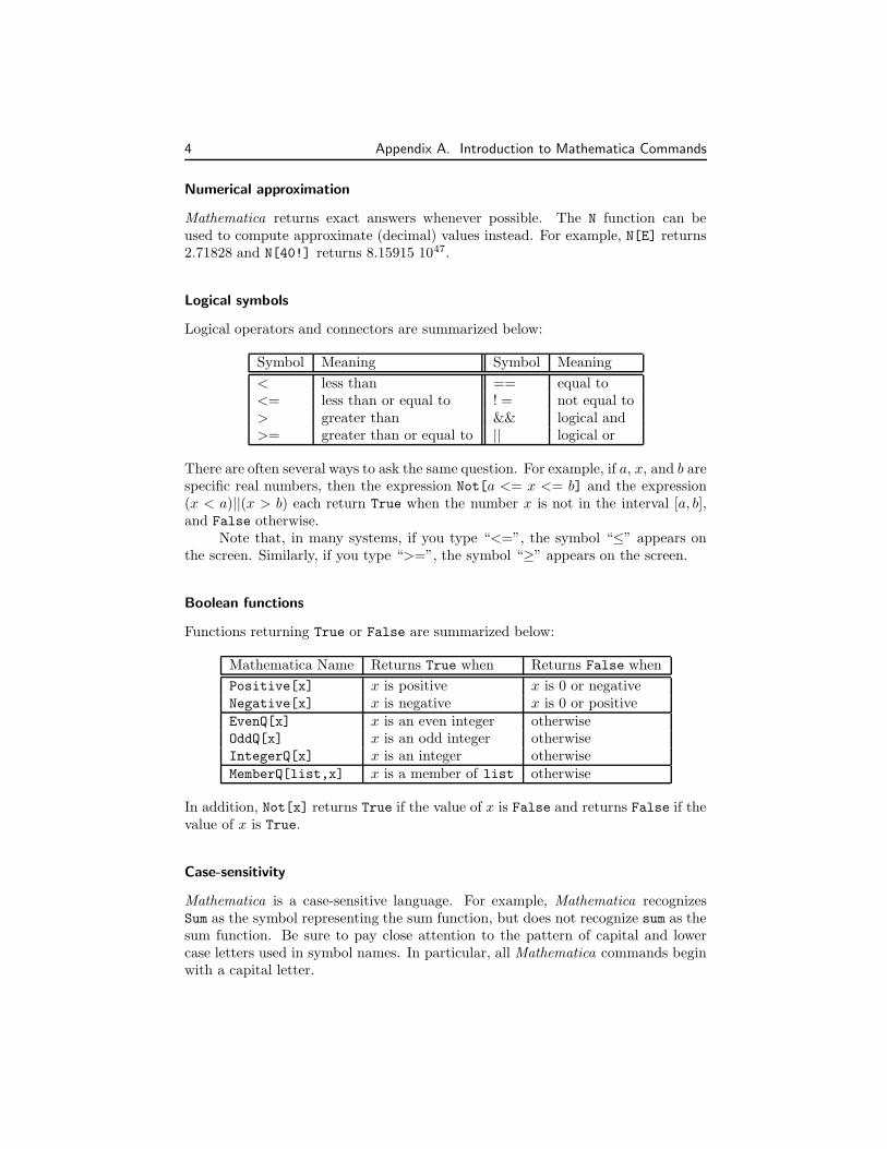
Logical symbols
Logical operators and connectors are summarized below:
Symbol Meaning Symbol Meaning
< less than == equal to<= less than or equal to ! = not equal to> greater than && logical and>= greater than or equal to || logical or
There are often several ways to ask the same question. For example, if a, x, and b arespecific real numbers, then the expression Not[a <= x <= b] and the expression(x < a)||(x > b) each return True when the number x is not in the interval [a, b],and False otherwise.
Note that, in many systems, if you type “<=”, the symbol “≤” appears onthe screen. Similarly, if you type “>=”, the symbol “≥” appears on the screen.
Boolean functions
Functions returning True or False are summarized below:
Mathematica Name Returns True when Returns False when
Positive[x] x is positive x is 0 or negativeNegative[x] x is negative x is 0 or positiveEvenQ[x] x is an even integer otherwiseOddQ[x] x is an odd integer otherwiseIntegerQ[x] x is an integer otherwiseMemberQ[list,x] x is a member of list otherwise
In addition, Not[x] returns True if the value of x is False and returns False if thevalue of x is True.
Case-sensitivity
Mathematica is a case-sensitive language. For example, Mathematica recognizesSum as the symbol representing the sum function, but does not recognize sum as thesum function. Be sure to pay close attention to the pattern of capital and lowercase letters used in symbol names. In particular, all Mathematica commands beginwith a capital letter.
A.1. Standard commands 5
A.1.2 User-defined variables and functions
Naming conventions for user-defined variables and functions, immediate and delayedassignments to symbols, echoing results to the screen, patterns and function defi-nitions, functions for clearing and removing symbols, and functions for conditionalstatements and building multi-step procedures are discussed below.
Naming conventions, assignment, echoing
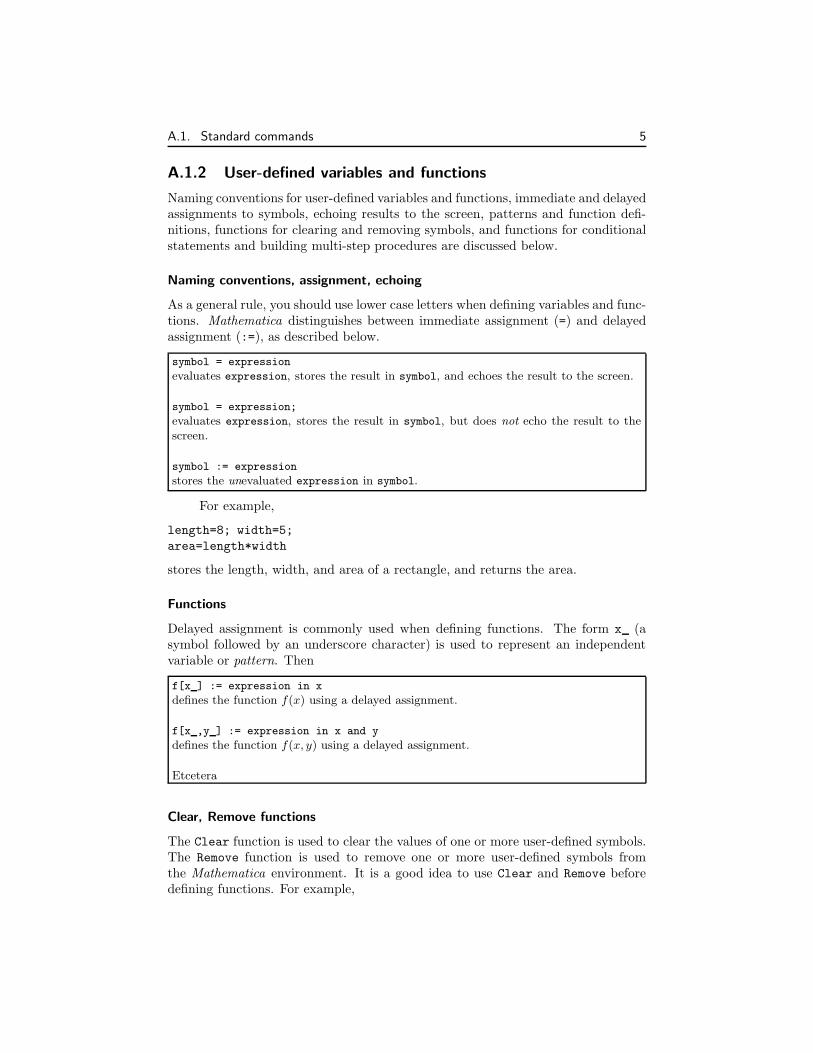
As a general rule, you should use lower case letters when defining variables and func-tions. Mathematica distinguishes between immediate assignment (=) and delayedassignment (:=), as described below.
symbol = expression
evaluates expression, stores the result in symbol, and echoes the result to the screen.
symbol = expression;
evaluates expression, stores the result in symbol, but does not echo the result to thescreen.
symbol := expression
stores the unevaluated expression in symbol.
For example,
length=8; width=5;
area=length*width
stores the length, width, and area of a rectangle, and returns the area.
Functions
Delayed assignment is commonly used when defining functions. The form x (asymbol followed by an underscore character) is used to represent an independentvariable or pattern. Then
f[x ] := expression in x
defines the function f(x) using a delayed assignment.
f[x ,y ] := expression in x and y
defines the function f(x, y) using a delayed assignment.
Etcetera
Clear, Remove functions
The Clear function is used to clear the values of one or more user-defined symbols.The Remove function is used to remove one or more user-defined symbols fromthe Mathematica environment. It is a good idea to use Clear and Remove beforedefining functions. For example,
6 Appendix A. Introduction to Mathematica Commands
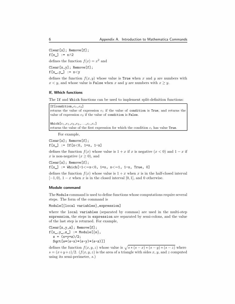
Clear[x]; Remove[f];
f[x ] := x∧2defines the function f(x) = x2 and
Clear[x,y]; Remove[f];
f[x ,y ] := x<y
defines the function f(x, y) whose value is True when x and y are numbers withx < y, and whose value is False when x and y are numbers with x ≥ y.
If, Which functions
The If and Which functions can be used to implement split-definition functions:
If[condition,e1,e2]
returns the value of expression e1 if the value of condition is True, and returns thevalue of expression e2 if the value of condition is False.
Which[c1,e1,c2,e2,. . .,cr,er]
returns the value of the first expression for which the condition ci has value True.
For example,
Clear[x]; Remove[f];
f[x ] := If[x<0, 1+x, 1-x]
defines the function f(x) whose value is 1 + x if x is negative (x < 0) and 1 − x ifx is non-negative (x ≥ 0), and
Clear[x]; Remove[f];
f[x ] := Which[-1<=x<0, 1+x, x<=1, 1-x, True, 0]
defines the function f(x) whose value is 1 + x when x is in the half-closed interval[−1, 0), 1 − x when x is in the closed interval [0, 1], and 0 otherwise.
Module command
The Module command is used to define functions whose computations require severalsteps. The form of the command is
Module[{local variables},expression]where the local variables (separated by commas) are used in the multi-stepexpression, the steps in expression are separated by semi-colons, and the valueof the last step is returned. For example,
Clear[x,y,z]; Remove[f];
f[x ,y ,z ] := Module[{s},s = (x+y+z)/2;
Sqrt[s*(s-x)*(s-y)*(s-z)]]
defines the function f(x, y, z) whose value is√
s ∗ (s − x) ∗ (s − y) ∗ (s − z) wheres = (x+y+z)/2. (f(x, y, z) is the area of a triangle with sides x, y, and z computedusing its semi-perimeter, s.)
A.1. Standard commands 7
A.1.3 Mathematica lists
The basic Mathematica data structure is the list (defined below). Functions forcomputing the length of a list, for sorting a list, for building lists, and for extractingelements and sublists are summarized below.
Definition of list
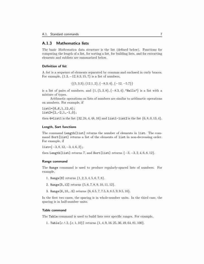
A list is a sequence of elements separated by commas and enclosed in curly braces.For example, {1.3,−12, 8.3, 15, 7} is a list of numbers,
{{5, 3.3}, {12.1, 2}, {−8.3, 4}, {−12,−5.7}}
is a list of pairs of numbers, and {1, {5, 3, 8}, {−8.3, 4}, "Hello"} is a list with amixture of types.
Arithmetic operations on lists of numbers are similar to arithmetic operationson numbers. For example, if
list1={8,6,1,12,4};list2={2,-2,1,-1,0};then 4*list1 is the list {32, 24, 4, 48, 16} and list1-list2 is the list {6, 8, 0, 13, 4}.
Length, Sort functions
The command Length[list] returns the number of elements in list. The com-mand Sort[list] returns a list of the elements of list in non-decreasing order.For example, if
list={−3, 8, 12,−3, 4, 6, 2};then Length[list] returns 7, and Sort[list] returns {−3,−3, 2, 4, 6, 8, 12}.
Range command
The Range command is used to produce regularly-spaced lists of numbers. Forexample,
1. Range[8] returns {1, 2, 3, 4, 5, 6, 7, 8}.
2. Range[5,12] returns {5, 6, 7, 8, 9, 10, 11, 12}.
3. Range[6,10,.5] returns {6, 6.5, 7, 7.5, 8, 8.5, 9, 9.5, 10}.
In the first two cases, the spacing is in whole-number units. In the third case, thespacing is in half-number units.
Table command
The Table command is used to build lists over specific ranges. For example,
1. Table[x∧ 2, {x, 1, 10}] returns {1, 4, 9, 16, 25, 36, 49, 64, 81, 100}.
8 Appendix A. Introduction to Mathematica Commands
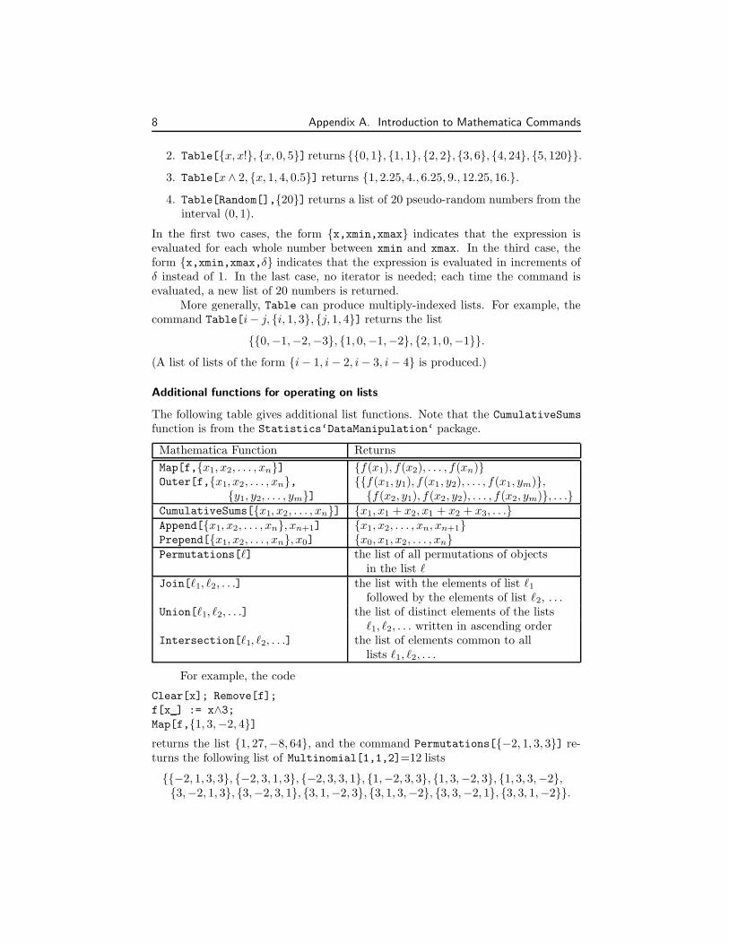
2. Table[{x, x!}, {x, 0, 5}] returns {{0, 1}, {1, 1}, {2, 2}, {3, 6}, {4, 24}, {5, 120}}.3. Table[x ∧ 2, {x, 1, 4, 0.5}] returns {1, 2.25, 4., 6.25, 9., 12.25, 16.}.4. Table[Random[],{20}] returns a list of 20 pseudo-random numbers from the
interval (0, 1).
In the first two cases, the form {x,xmin,xmax} indicates that the expression isevaluated for each whole number between xmin and xmax. In the third case, theform {x,xmin,xmax,δ} indicates that the expression is evaluated in increments ofδ instead of 1. In the last case, no iterator is needed; each time the command isevaluated, a new list of 20 numbers is returned.
More generally, Table can produce multiply-indexed lists. For example, thecommand Table[i− j, {i, 1, 3}, {j, 1, 4}] returns the list
{{0,−1,−2,−3}, {1, 0,−1,−2}, {2, 1, 0,−1}}.(A list of lists of the form {i− 1, i − 2, i− 3, i − 4} is produced.)
Additional functions for operating on lists
The following table gives additional list functions. Note that the CumulativeSums
function is from the Statistics‘DataManipulation‘ package.
Mathematica Function Returns
Map[f,{x1, x2, . . . , xn}] {f(x1), f(x2), . . . , f(xn)}Outer[f,{x1, x2, . . . , xn}, {{f(x1, y1), f(x1, y2), . . . , f(x1, ym)},
{y1, y2, . . . , ym}] {f(x2, y1), f(x2, y2), . . . , f(x2, ym)}, . . .}CumulativeSums[{x1, x2, . . . , xn}] {x1, x1 + x2, x1 + x2 + x3, . . .}Append[{x1, x2, . . . , xn}, xn+1] {x1, x2, . . . , xn, xn+1}Prepend[{x1, x2, . . . , xn}, x0] {x0, x1, x2, . . . , xn}Permutations[`] the list of all permutations of objects
in the list `Join[`1, `2, . . .] the list with the elements of list `1
followed by the elements of list `2, . . .Union[`1, `2, . . .] the list of distinct elements of the lists
`1, `2, . . . written in ascending orderIntersection[`1, `2, . . .] the list of elements common to all
lists `1, `2, . . .
For example, the code
Clear[x]; Remove[f];
f[x ] := x∧3;Map[f,{1, 3,−2, 4}]returns the list {1, 27,−8, 64}, and the command Permutations[{−2, 1, 3, 3}] re-turns the following list of Multinomial[1,1,2]=12 lists
{{−2, 1, 3, 3}, {−2, 3, 1, 3}, {−2, 3, 3, 1}, {1,−2, 3, 3}, {1, 3,−2, 3}, {1, 3, 3,−2},{3,−2, 1, 3}, {3,−2, 3, 1}, {3, 1,−2, 3}, {3, 1, 3,−2}, {3, 3,−2, 1}, {3, 3, 1,−2}}.
A.1. Standard commands 9
Select function
The Select function can be used to choose elements of a list satisfying a givencriterion. For example,
Clear[x]; Remove[f];
f[x ] := x < 10;
Select[{18, 3,−2, 12, 5,−19, 3},f]returns the sublist of elements less than 10, {3,−2, 5,−19, 3}.
Note that “unnamed” (or pure) functions are often used in Select commandsin the laboratory problems. For example, the single command
Select[{18, 3,−2, 12, 5,−19, 3},(#<10)&]gives the same result as above. (The & says that the expression in parentheses isan unnamed function whose argument is #.)
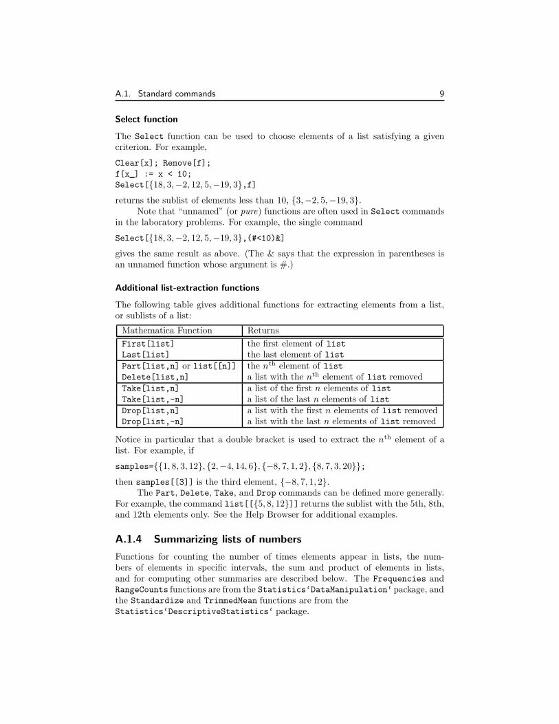
Additional list-extraction functions
The following table gives additional functions for extracting elements from a list,or sublists of a list:
Mathematica Function Returns
First[list] the first element of listLast[list] the last element of list
Part[list,n] or list[[n]] the nth element of listDelete[list,n] a list with the nth element of list removedTake[list,n] a list of the first n elements of listTake[list,-n] a list of the last n elements of listDrop[list,n] a list with the first n elements of list removedDrop[list,-n] a list with the last n elements of list removed
Notice in particular that a double bracket is used to extract the nth element of alist. For example, if
samples={{1, 8, 3, 12}, {2,−4, 14, 6}, {−8, 7, 1, 2}, {8, 7, 3, 20}};then samples[[3]] is the third element, {−8, 7, 1, 2}.
The Part, Delete, Take, and Drop commands can be defined more generally.For example, the command list[[{5, 8, 12}]] returns the sublist with the 5th, 8th,and 12th elements only. See the Help Browser for additional examples.
A.1.4 Summarizing lists of numbers
Functions for counting the number of times elements appear in lists, the num-bers of elements in specific intervals, the sum and product of elements in lists,and for computing other summaries are described below. The Frequencies andRangeCounts functions are from the Statistics‘DataManipulation‘package, andthe Standardize and TrimmedMean functions are from theStatistics‘DescriptiveStatistics‘ package.
10 Appendix A. Introduction to Mathematica Commands
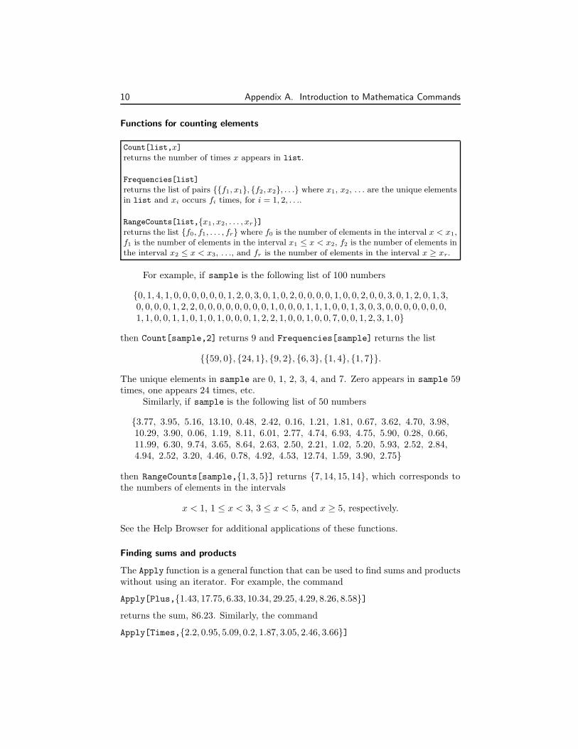
Functions for counting elements
Count[list,x]returns the number of times x appears in list.
Frequencies[list]
returns the list of pairs {{f1, x1}, {f2, x2}, . . .} where x1, x2, . . . are the unique elementsin list and xi occurs fi times, for i = 1, 2, . . ..
RangeCounts[list,{x1 , x2, . . . , xr}]returns the list {f0, f1, . . . , fr} where f0 is the number of elements in the interval x < x1,f1 is the number of elements in the interval x1 ≤ x < x2, f2 is the number of elements inthe interval x2 ≤ x < x3, . . ., and fr is the number of elements in the interval x ≥ xr.
For example, if sample is the following list of 100 numbers
{0, 1, 4, 1, 0, 0, 0, 0, 0, 0, 1, 2, 0, 3, 0, 1, 0, 2, 0, 0, 0, 0, 1, 0, 0, 2, 0, 0, 3, 0, 1, 2, 0, 1, 3,0, 0, 0, 0, 1, 2, 2, 0, 0, 0, 0, 0, 0, 0, 0, 1, 0, 0, 0, 1, 1, 1, 0, 0, 1, 3, 0, 3, 0, 0, 0, 0, 0, 0, 0,1, 1, 0, 0, 1, 1, 0, 1, 0, 1, 0, 0, 0, 1, 2, 2, 1, 0, 0, 1, 0, 0, 7, 0, 0, 1, 2, 3, 1, 0}
then Count[sample,2] returns 9 and Frequencies[sample] returns the list
{{59, 0}, {24, 1}, {9, 2}, {6, 3}, {1, 4}, {1, 7}}.
The unique elements in sample are 0, 1, 2, 3, 4, and 7. Zero appears in sample 59times, one appears 24 times, etc.
Similarly, if sample is the following list of 50 numbers
{3.77, 3.95, 5.16, 13.10, 0.48, 2.42, 0.16, 1.21, 1.81, 0.67, 3.62, 4.70, 3.98,10.29, 3.90, 0.06, 1.19, 8.11, 6.01, 2.77, 4.74, 6.93, 4.75, 5.90, 0.28, 0.66,11.99, 6.30, 9.74, 3.65, 8.64, 2.63, 2.50, 2.21, 1.02, 5.20, 5.93, 2.52, 2.84,4.94, 2.52, 3.20, 4.46, 0.78, 4.92, 4.53, 12.74, 1.59, 3.90, 2.75}
then RangeCounts[sample,{1, 3, 5}] returns {7, 14, 15, 14}, which corresponds tothe numbers of elements in the intervals
x < 1, 1 ≤ x < 3, 3 ≤ x < 5, and x ≥ 5, respectively.
See the Help Browser for additional applications of these functions.
Finding sums and products
The Apply function is a general function that can be used to find sums and productswithout using an iterator. For example, the command
Apply[Plus,{1.43, 17.75, 6.33, 10.34, 29.25, 4.29, 8.26, 8.58}]returns the sum, 86.23. Similarly, the command
Apply[Times,{2.2, 0.95, 5.09, 0.2, 1.87, 3.05, 2.46, 3.66}]
A.1. Standard commands 11
returns the product, 109.258.Note that the shorthand Plus@@list can be used to find the sum of the
numbers in list, and the shorthand Times@@list can be used to find the productof the numbers in list.
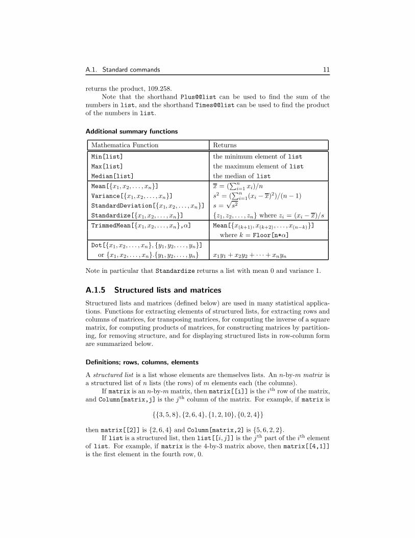
Additional summary functions
Mathematica Function Returns
Min[list] the minimum element of list
Max[list] the maximum element of list
Median[list] the median of list
Mean[{x1, x2, . . . , xn}] x = (∑n
i=1 xi)/n
Variance[{x1, x2, . . . , xn}] s2 = (∑n
i=1(xi − x)2)/(n − 1)
StandardDeviation[{x1, x2, . . . , xn}] s =√
s2
Standardize[{x1, x2, . . . , xn}] {z1, z2, . . . , zn} where zi = (xi − x)/s
TrimmedMean[{x1, x2, . . . , xn},α] Mean[{x(k+1), x(k+2), . . . , x(n−k)}]where k = Floor[n*α]
Dot[{x1, x2, . . . , xn}, {y1, y2, . . . , yn}]or {x1, x2, . . . , xn}.{y1, y2, . . . , yn} x1y1 + x2y2 + · · · + xnyn
Note in particular that Standardize returns a list with mean 0 and variance 1.
A.1.5 Structured lists and matrices
Structured lists and matrices (defined below) are used in many statistical applica-tions. Functions for extracting elements of structured lists, for extracting rows andcolumns of matrices, for transposing matrices, for computing the inverse of a squarematrix, for computing products of matrices, for constructing matrices by partition-ing, for removing structure, and for displaying structured lists in row-column formare summarized below.
Definitions; rows, columns, elements
A structured list is a list whose elements are themselves lists. An n-by-m matrix isa structured list of n lists (the rows) of m elements each (the columns).
If matrix is an n-by-m matrix, then matrix[[i]] is the ith row of the matrix,and Column[matrix,j] is the jth column of the matrix. For example, if matrix is
{{3, 5, 8}, {2, 6, 4}, {1, 2, 10}, {0, 2, 4}}
then matrix[[2]] is {2, 6, 4} and Column[matrix,2] is {5, 6, 2, 2}.If list is a structured list, then list[[i, j]] is the jth part of the ith element
of list. For example, if matrix is the 4-by-3 matrix above, then matrix[[4,1]]
is the first element in the fourth row, 0.
12 Appendix A. Introduction to Mathematica Commands
Exchanging rows and columns
The Transpose function can be used to exchange the rows and columns of an n-by-m matrix. For the 4-by-3 matrix above, for example, Transpose[matrix] returnsthe following 3-by-4 matrix
{{3, 2, 1, 0}, {5, 6, 2, 2}, {8, 4, 10, 4}}.
Inverse of a matrix, product of matrices
If matrix is an n-by-n matrix of numbers, then Inverse[matrix] returns the in-verse of the matrix (if it exists). For example, the commands
matrix = {{2, 5}, {1, 3}};Inverse[matrix]
return the inverse of the 2-by-2 matrix, {{3,−5}, {−1, 2}}.If m1 is an n-by-m matrix of numbers and m2 is an m-by-p matrix of numbers,
then the command m1.m2 returns the n-by-p matrix product. For example, thecommands
m1={{8, 0, 2}, {1,−4, 1}};m2={{4, 1}, {0, 3}, {−1,−3}};m1.m2
return the 2-by-2 matrix {{30, 2}, {3,−14}}. Similarly, given the 2-by-2 invertiblematrix above, the command matrix.Inverse[matrix] returns the 2-by-2 identitymatrix, {{1, 0}, {0, 1}}.
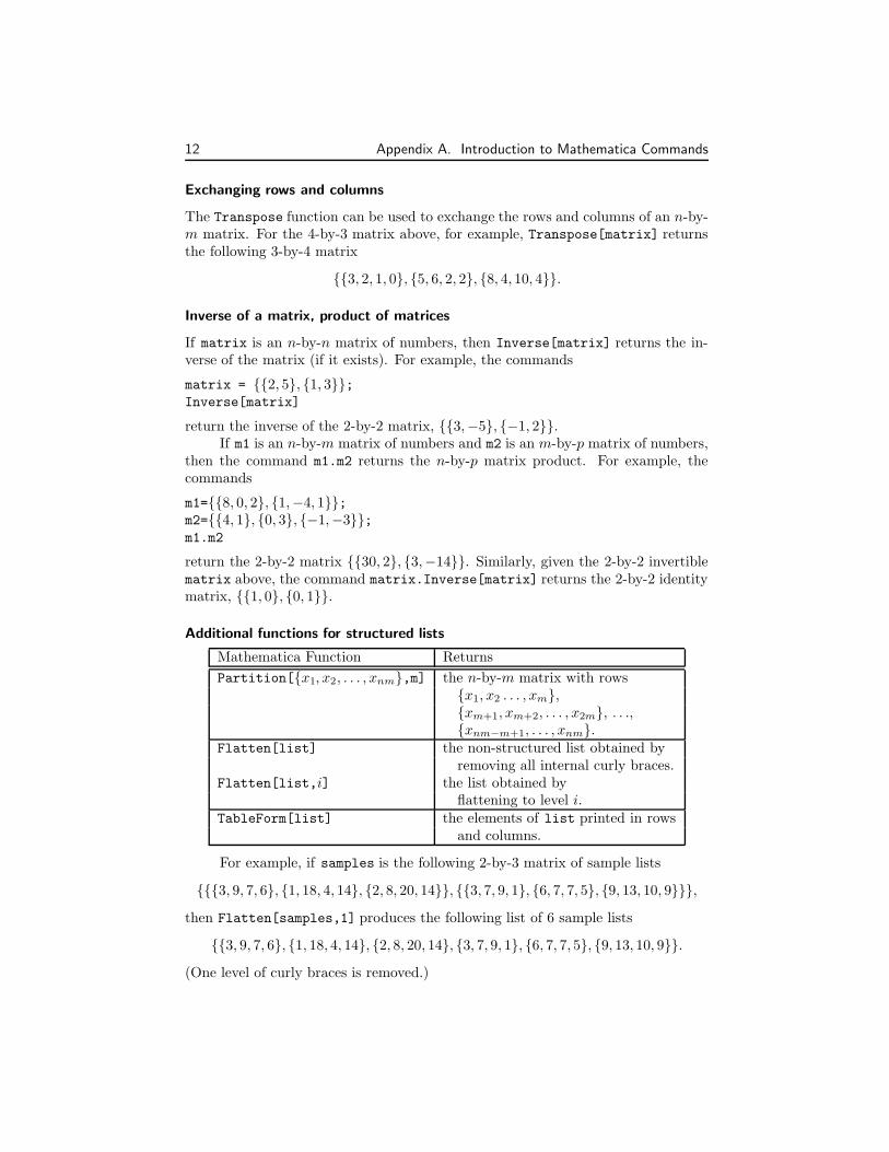
Additional functions for structured lists
Mathematica Function Returns
Partition[{x1, x2, . . . , xnm},m] the n-by-m matrix with rows{x1, x2 . . . , xm},{xm+1, xm+2, . . . , x2m}, . . .,{xnm−m+1, . . . , xnm}.
Flatten[list] the non-structured list obtained byremoving all internal curly braces.
Flatten[list,i] the list obtained byflattening to level i.
TableForm[list] the elements of list printed in rowsand columns.
For example, if samples is the following 2-by-3 matrix of sample lists
{{{3, 9, 7, 6}, {1, 18, 4, 14}, {2, 8, 20, 14}}, {{3, 7, 9, 1}, {6, 7, 7, 5}, {9, 13, 10, 9}}},
then Flatten[samples,1] produces the following list of 6 sample lists
{{3, 9, 7, 6}, {1, 18, 4, 14}, {2, 8, 20, 14}, {3, 7, 9, 1}, {6, 7, 7, 5}, {9, 13, 10, 9}}.
(One level of curly braces is removed.)
A.1. Standard commands 13
-3 -2 -1 1 2 3x
0.2
0.4
0.6
0.8
1y
-3 -2 -1 1 2 3 x
0.2
0.4
0.6
0.8
1y
-3 -2 -1 1 2 3 x
0.2
0.4
0.6
0.8
1y
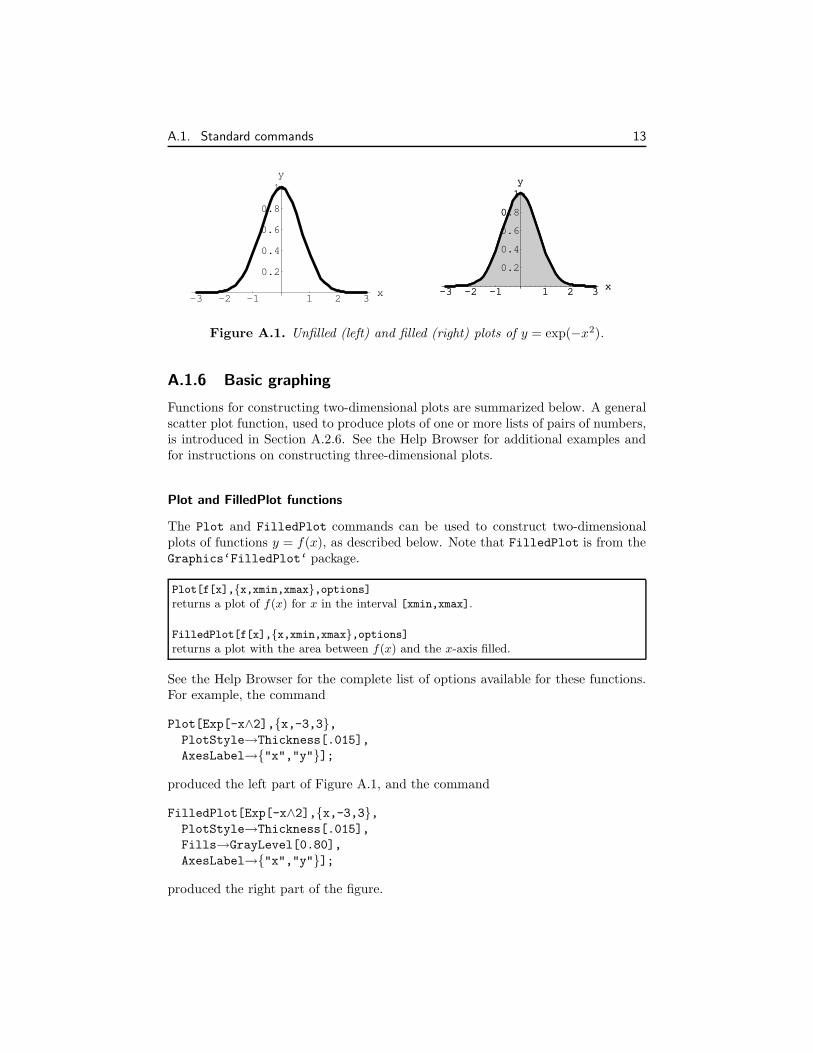
Figure A.1. Unfilled (left) and filled (right) plots of y = exp(−x2).
A.1.6 Basic graphing
Functions for constructing two-dimensional plots are summarized below. A generalscatter plot function, used to produce plots of one or more lists of pairs of numbers,is introduced in Section A.2.6. See the Help Browser for additional examples andfor instructions on constructing three-dimensional plots.
Plot and FilledPlot functions
The Plot and FilledPlot commands can be used to construct two-dimensionalplots of functions y = f(x), as described below. Note that FilledPlot is from theGraphics‘FilledPlot‘ package.
Plot[f[x],{x,xmin,xmax},options]returns a plot of f(x) for x in the interval [xmin,xmax].
FilledPlot[f[x],{x,xmin,xmax},options]returns a plot with the area between f(x) and the x-axis filled.
See the Help Browser for the complete list of options available for these functions.For example, the command
Plot[Exp[-x∧2],{x,-3,3},PlotStyle→Thickness[.015],
AxesLabel→{"x","y"}];
produced the left part of Figure A.1, and the command
FilledPlot[Exp[-x∧2],{x,-3,3},PlotStyle→Thickness[.015],
Fills→GrayLevel[0.80],
AxesLabel→{"x","y"}];
produced the right part of the figure.
14 Appendix A. Introduction to Mathematica Commands
A.1.7 Derivatives and integrals
Functions for computing derivatives and partial derivatives, and for computing def-inite and indefinite integrals are summarized below.
Derivatives and partial derivatives
The command D[expression,x] returns the derivative (or partial derivative) ofexpressionwith respect to x. The expression can contain any number of symbols.For example, if expression is the polynomial
7 + a x2 − 2 b x y + 15 c x3 z2,
then D[expression,x] returns 2 a x − 2 b y + 45 c x2 z2.For functions of one variable, the shorthand f′[x] can also be used to return
the derivative. For example,
Clear[x]; Remove[f];
f[x ] := Sin[2*x];
f′[x]
returns 2 Cos[2 x]. Similarly, f′′[x] returns -4 Sin[2 x].
Definite and indefinite integrals
The Integrate command is used to compute antiderivatives and to compute definiteintegrals. For the function above, for example, Integrate[f[x],x] returns theantiderivative -Cos[2 x]/2 and the command
Integrate[f[x], {x,0,Pi/4}]returns 1/2. (The area under the curve y = f(x) and above the interval [0, π/4] onthe the x-axis is 1/2 square units.)
More generally, Integrate can be used to compute multiple integrals. Forexample, the commands
Clear[x,y];
Integrate[x∧2 + 4y∧2, {x,0,3}, {y,0,x}]return 189/4. (The volume under the surface z = x2 +4y2 and above the triangularregion in the xy-plane with corners (0, 0), (3, 0), (3, 3) is 189/4 cubic units.)
Assumptions in definite integrals
The option Assumptions is used to specify conditions on symbols in the integrand.For example, the commands
Clear[a,x];
Integrate[Exp[-a*x], {x,0,∞}, Assumptions → a> 0]
return 1/a. (If a > 0, then the value of the integral exists and equals 1/a.) See theHelp Browser for additional situations where the Assumptions option is used.
A.1. Standard commands 15
A.1.8 Symbolic operations and solving equations
Functions for working with polynomial and rational expressions, for replacing oc-currences of one subexpression with another, and for solving equations exactly andapproximately are summarized below.
Working with polynomial and rational expressions
Mathematica Function Action
Expand[expression] multiplies out the products and powersin expression.
Factor[expression] returns an equivalent product of factors.Together[expression] combines terms of expression over a
common denominator.Apart[expression] splits expression into partial fractions.Simplify[expression] returns a simplied form.Coefficient[polynomial,x,r] returns the coefficient of xr in the
expanded polynomial.
For example, the command
Clear[t];
expression = Expand[(1 + t)∧8]returns the polynomial
1 + 8 t + 28 t2 + 56 t3 + 70 t4 + 56 t5 + 28 t6 + 8 t7 + t8
and the command Coefficient[expression,t,4] returns 70.
Replacing subexpressions
The ReplaceAll function is used to replace all occurrences of one subexpressionwith another (or all occurrences of many subexpressions with others).
Mathematica Function Action
ReplaceAll[expression,x→a] replaces all occurrences of x inor expression /. x→a expression with a.
ReplaceAll[expression,{x→ a, y → b, . . .}] replaces all occurrences ofor expression /. {x → a, y → b, . . .} x with a, y with b, etc.
An expression of the form lhs→rhs is called a rule. The rule lhs→rhs means“replace the lefthand side (lhs) with the value of the righthand side (rhs).”
For example, if expression contains the polynomial
5 x2 − 15 x y + 27 z2
then the command
expression /. x→(y+z)∧2returns the polynomial
27 z2 − 15 y (y + z)2
+ 5 (y + z)4
16 Appendix A. Introduction to Mathematica Commands
Solving equations
The Solve and NSolve functions can be used to find solutions to polynomial andrational equations:
Mathematica Function Action
Solve[equation, x] solves equation for x.NSolve[equation,x] solves equation for x numerically.Solve[{e1, e2, . . .}, {x1, x2, . . .}] solves the system of equations e1, e2, . . .,
for variables x1, x2, . . ..NSolve[{e1, e2, . . .}, {x1, x2, . . .}] solves the system numerically.
For example, the command
Solve[240+10*x-45*x∧2+5*x∧3==0,x]
returns the list of replacement rules {{x → −2}, {x → 3}, {x → 8}}. (Each rulecorresponds to a root of the polynomial equation 240+10x−45x2+5x3 = 0.) Notethat a double equal sign (==) is used in the first argument of Solve.
FindRoot command
More generally, FindRoot can be used to find approximate solutions to equationsusing a sequence of iterations:
FindRoot[equation,{x, x0}]searches for a numerical solution to equation starting from x = x0.
FindRoot[{e1 , e2, . . .}, {x, x0}, {y, y0}, . . .]searches for a numerical solution to the system of equations e1, e2, . . . in variables x, y,. . . using the starting values x = x0, y = y0, . . ..
For example, the graphs of y = x+4 and y = ex/3 have a point of intersectionbetween x = 6 and x = 8. Using x = 7 as a starting value, the command
FindRoot[x+4 == Exp[x/3], {x,7}]
returns the list {x → 7.26514}, indicating that the point of intersection has x-coordinate approximately 7.26514. Note that a double equal sign (==) is used inthe first argument of FindRoot.
A.1.9 Univariate probability distributions
The following tables give information on the discrete and continuous families ofdistributions used in the book. The information is from the
Statistics‘DiscreteDistributions‘ andStatistics‘ContinuousDistributions‘ packages.
A.1. Standard commands 17
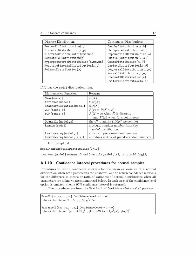
Discrete Distributions Continuous Distributions
BernoulliDistribution[p] CauchyDistribution[a,b]
BinomialDistribution[n,p] ChiSquareDistribution[n]
DiscreteUniformDistribution[n] ExponentialDistribution[λ]GeometricDistribution[p] FRatioDistribution[ν1,ν2]
HypergeometricDistribution[n,mm,nn] GammaDistribution[α,β]NegativeBinomialDistribution[r,p] LaplaceDistribution[µ,β]PoissonDistribution[λ] LognormalDistribution[µ,σ]
NormalDistribution[µ,σ]StudentTDistribution[n]
UniformDistribution[a,b]
If X has the model distribution, then
Mathematica Function Returns
Mean[model] E(X)Variance[model] V ar(X)StandardDeviation[model] SD(X)CDF[model,x] F (x) = P (X ≤ x)PDF[model,x] P (X = x) when X is discrete,
and F ′(x) when X is continuous.
Quantile[model,p] the pth quantile (100pth percentile)Random[model] a pseudo-random number from the
model distributionRandomArray[model,r] a list of r pseudo-random numbersRandomArray[model,{r, s}] an r-by-s matrix of pseudo-random numbers
For example, if
model=ExponentialDistribution[1/10];
then Mean[model] returns 10 and Quantile[model,1/2] returns 10 Log[2].
A.1.10 Confidence interval procedures for normal samples
Procedures to return confidence intervals for the mean or variance of a normaldistribution when both parameters are unknown, and to return confidence intervalsfor the difference in means or ratio of variances of normal distributions when allparameters are unknown are summarized below. In each case, if the confidence leveloption is omitted, then a 95% confidence interval is returned.
The procedures are from the Statistics‘ConfidenceIntervals‘ package.
MeanCI[{x1, x2, . . . , xn},ConfidenceLevel→ 1 − α]
returns the interval x ± tn−1(α/2)√
s2/n.
VarianceCI[{x1 , x2, . . . , xn},ConfidenceLevel→ 1 − α]returns the interval
[(n − 1)s2/χ2
n−1(1 − α/2), (n − 1)s2/χ2n−1(α/2)
].
18 Appendix A. Introduction to Mathematica Commands
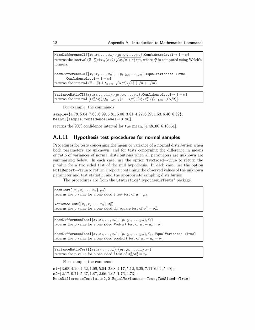
MeanDifferenceCI[{x1 , x2, . . . , xn},{y1, y2, . . . , ym},ConfidenceLevel→ 1 − α]
returns the interval (x−y)±tdf (α/2)√
s2x/n + s2
y/m, where df is computed using Welch’sformula.
MeanDifferenceCI[{x1 , x2, . . . , xn}, {y1, y2, . . . , ym},EqualVariances→True,
ConfidenceLevel→ 1 − α]returns the interval (x − y) ± tn+m−2(α/2)
√s2
p (1/n + 1/m).
VarianceRatioCI[{x1 , x2, . . . , xn},{y1, y2, . . . , ym},ConfidenceLevel→ 1 − α]returns the interval
[(s2
x/s2y)/fn−1,m−1(1 − α/2), (s2
x/s2y)/fn−1,m−1(α/2)
].
For example, the commands
sample={4.79, 5.04, 7.63, 6.99, 5.81, 5.08, 3.81, 4.27, 6.27, 1.53, 6.46, 6.32};MeanCI[sample,ConfidenceLevel→0.90]
returns the 90% confidence interval for the mean, [4.48106, 6.18561].
A.1.11 Hypothesis test procedures for normal samples
Procedures for tests concerning the mean or variance of a normal distribution whenboth parameters are unknown, and for tests concerning the difference in meansor ratio of variances of normal distributions when all parameters are unknown aresummarized below. In each case, use the option TwoSided→True to return thep value for a two sided test of the null hypothesis. In each case, use the optionFullReport→True to return a report containing the observed values of the unknownparameter and test statistic, and the appropriate sampling distribution.
The procedures are from the Statistics‘HypothesisTests‘ package.
MeanTest[{x1, x2, . . . , xn}, µ0]
returns the p value for a one sided t test test of µ = µ0.
VarianceTest[{x1 , x2, . . . , xn}, σ20]
returns the p value for a one sided chi square test of σ2 = σ20 .
MeanDifferenceTest[{x1 , x2, . . . , xn},{y1, y2, . . . , ym}, δ0]
returns the p value for a one sided Welch t test of µx − µy = δ0.
MeanDifferenceTest[{x1 , x2, . . . , xn},{y1, y2, . . . , ym}, δ0, EqualVariances→True]
returns the p value for a one sided pooled t test of µx − µy = δ0.
VarianceRatioTest[{x1 , x2, . . . , xn},{y1, y2, . . . , ym},r0]
returns the p value for a one sided f test of σ2x/σ2
y = r0.
For example, the commands
s1={3.68, 4.29, 4.62, 1.09, 5.54, 2.68, 4.17, 5.12, 6.25, 7.11, 6.94, 5.49};s2={2.17, 0.71, 5.67, 1.87, 2.06, 1.05, 1.76, 4.73};MeanDifferenceTest[s1,s2,0,EqualVariances→True,TwoSided→True]
A.1. Standard commands 19
return the p value for a two sided pooled t test of the equality of means (δo = 0) asa Mathematica rule, TwoSidedPValue→0.0113969.
A.1.12 Linear and nonlinear least squares
Functions for finding linear and nonlinear least squares formulas, and for linearregression analyses are summarized below.
Fit function
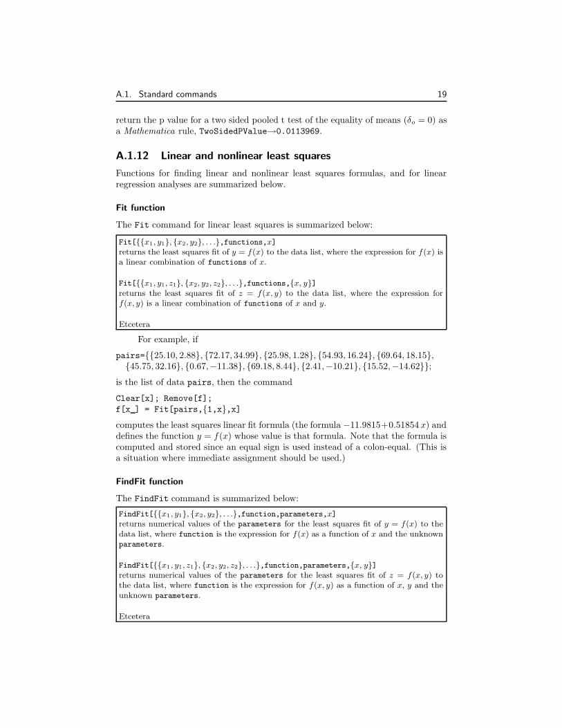
The Fit command for linear least squares is summarized below:
Fit[{{x1, y1}, {x2, y2}, . . .},functions,x]returns the least squares fit of y = f(x) to the data list, where the expression for f(x) isa linear combination of functions of x.
Fit[{{x1, y1, z1}, {x2, y2, z2}, . . .},functions,{x, y}]returns the least squares fit of z = f(x, y) to the data list, where the expression forf(x, y) is a linear combination of functions of x and y.
Etcetera
For example, if
pairs={{25.10, 2.88}, {72.17, 34.99}, {25.98, 1.28}, {54.93, 16.24}, {69.64, 18.15},{45.75, 32.16}, {0.67,−11.38}, {69.18, 8.44}, {2.41,−10.21}, {15.52,−14.62}};
is the list of data pairs, then the command
Clear[x]; Remove[f];
f[x ] = Fit[pairs,{1,x},x]computes the least squares linear fit formula (the formula −11.9815+0.51854 x) anddefines the function y = f(x) whose value is that formula. Note that the formula iscomputed and stored since an equal sign is used instead of a colon-equal. (This isa situation where immediate assignment should be used.)
FindFit function
The FindFit command is summarized below:
FindFit[{{x1 , y1}, {x2, y2}, . . .},function,parameters,x]returns numerical values of the parameters for the least squares fit of y = f(x) to thedata list, where function is the expression for f(x) as a function of x and the unknownparameters.
FindFit[{{x1 , y1, z1}, {x2, y2, z2}, . . .},function,parameters,{x, y}]returns numerical values of the parameters for the least squares fit of z = f(x, y) tothe data list, where function is the expression for f(x, y) as a function of x, y and theunknown parameters.
Etcetera
20 Appendix A. Introduction to Mathematica Commands
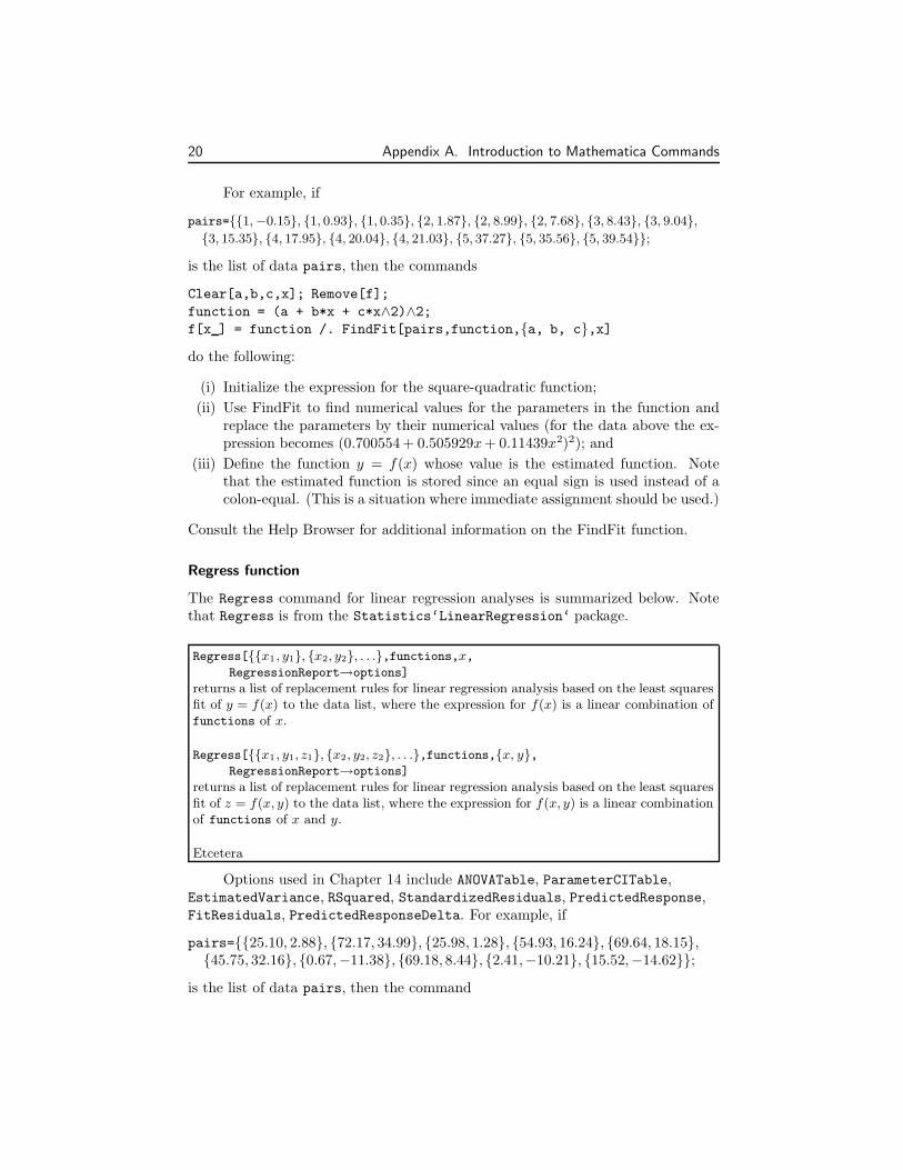
For example, if
pairs={{1,−0.15}, {1, 0.93}, {1, 0.35}, {2, 1.87}, {2, 8.99}, {2, 7.68}, {3, 8.43}, {3, 9.04},
{3, 15.35}, {4, 17.95}, {4, 20.04}, {4, 21.03}, {5, 37.27}, {5, 35.56}, {5, 39.54}};
is the list of data pairs, then the commands
Clear[a,b,c,x]; Remove[f];
function = (a + b*x + c*x∧2)∧2;f[x ] = function /. FindFit[pairs,function,{a, b, c},x]
do the following:
(i) Initialize the expression for the square-quadratic function;
(ii) Use FindFit to find numerical values for the parameters in the function andreplace the parameters by their numerical values (for the data above the ex-pression becomes (0.700554 + 0.505929x + 0.11439x2)2); and
(iii) Define the function y = f(x) whose value is the estimated function. Notethat the estimated function is stored since an equal sign is used instead of acolon-equal. (This is a situation where immediate assignment should be used.)
Consult the Help Browser for additional information on the FindFit function.
Regress function
The Regress command for linear regression analyses is summarized below. Notethat Regress is from the Statistics‘LinearRegression‘ package.
Regress[{{x1 , y1}, {x2, y2}, . . .},functions,x,RegressionReport→options]
returns a list of replacement rules for linear regression analysis based on the least squaresfit of y = f(x) to the data list, where the expression for f(x) is a linear combination offunctions of x.
Regress[{{x1 , y1, z1}, {x2, y2, z2}, . . .},functions,{x, y},RegressionReport→options]
returns a list of replacement rules for linear regression analysis based on the least squaresfit of z = f(x, y) to the data list, where the expression for f(x, y) is a linear combinationof functions of x and y.
Etcetera
Options used in Chapter 14 include ANOVATable, ParameterCITable,EstimatedVariance, RSquared, StandardizedResiduals, PredictedResponse,FitResiduals, PredictedResponseDelta. For example, if
pairs={{25.10, 2.88}, {72.17, 34.99}, {25.98, 1.28}, {54.93, 16.24}, {69.64, 18.15},{45.75, 32.16}, {0.67,−11.38}, {69.18, 8.44}, {2.41,−10.21}, {15.52,−14.62}};
is the list of data pairs, then the command
A.2. Custom tools 21
Clear[x];
results = Regress[pairs,{1, x},x,RegressionReport→{ANOVATable, RSquared}];
does the following:
(i) Carries out a linear regression analysis where the hypothesized conditionalexpectation is E(Y |X = x) = β0 + β1x; and
(ii) Stores a list containing the analysis of variance f test and the coefficient ofdetermination in results.
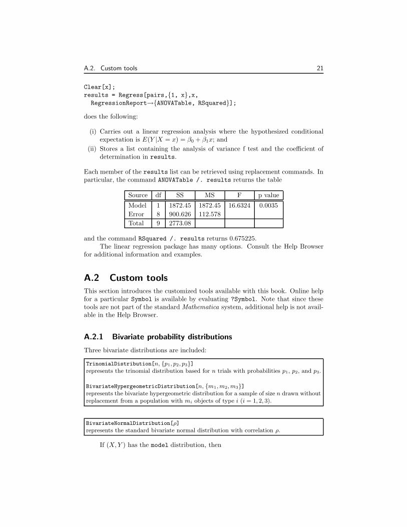
Each member of the results list can be retrieved using replacement commands. Inparticular, the command ANOVATable /. results returns the table
Source df SS MS F p value
Model 1 1872.45 1872.45 16.6324 0.0035
Error 8 900.626 112.578
Total 9 2773.08
and the command RSquared /. results returns 0.675225.The linear regression package has many options. Consult the Help Browser
for additional information and examples.
A.2 Custom tools
This section introduces the customized tools available with this book. Online helpfor a particular Symbol is available by evaluating ?Symbol. Note that since thesetools are not part of the standard Mathematica system, additional help is not avail-able in the Help Browser.
A.2.1 Bivariate probability distributions
Three bivariate distributions are included:
TrinomialDistribution[n, {p1, p2, p3}]represents the trinomial distribution based for n trials with probabilities p1, p2, and p3.
BivariateHypergeometricDistribution[n, {m1, m2, m3}]represents the bivariate hypergeometric distribution for a sample of size n drawn withoutreplacement from a population with mi objects of type i (i = 1, 2, 3).
BivariateNormalDistribution[ρ]represents the standard bivariate normal distribution with correlation ρ.
If (X, Y ) has the model distribution, then
22 Appendix A. Introduction to Mathematica Commands
Mathematica Function Returns
Mean[model] {E(X), E(Y )}Variance[model] {V ar(X), V ar(Y )}StandardDeviation[model] {SD(X), SD(Y )}Correlation[model] Corr(X, Y )
PDF[model,x,y] the joint PDF at (x, y)
Random[model] a pseudo-random pair from the
model distribution
RandomArray[model,r] a list of r pseudo-random pairs
RandomArray[model,{r, s}] an r-by-s matrix of pseudo-random pairs
For example, if
model=TrinomialDistribution[10,{0.2, 0.3, 0.5}];then Mean[model] returns {2., 3.} and Correlation[model] returns −0.327327.
A.2.2 Multinomial distribution and goodness-of-fit
The multinomial model is included:
MultinomialDistribution[n, {p1, p2, . . . , pk}]represents the multinomial distribution for n trials with probabilities p1, p2, . . ., pk.
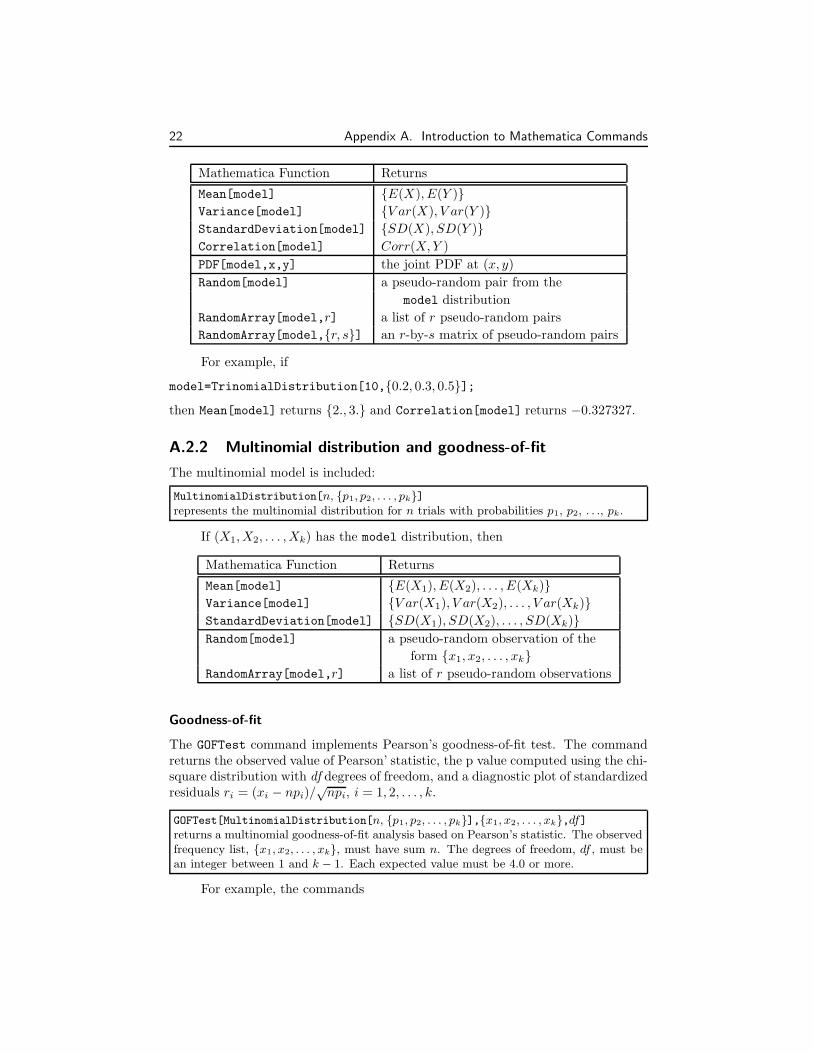
If (X1, X2, . . . , Xk) has the model distribution, then
Mathematica Function Returns
Mean[model] {E(X1), E(X2), . . . , E(Xk)}Variance[model] {V ar(X1), V ar(X2), . . . , V ar(Xk)}StandardDeviation[model] {SD(X1), SD(X2), . . . , SD(Xk)}Random[model] a pseudo-random observation of the
form {x1, x2, . . . , xk}RandomArray[model,r] a list of r pseudo-random observations
Goodness-of-fit
The GOFTest command implements Pearson’s goodness-of-fit test. The commandreturns the observed value of Pearson’ statistic, the p value computed using the chi-square distribution with df degrees of freedom, and a diagnostic plot of standardizedresiduals ri = (xi − npi)/
√npi, i = 1, 2, . . . , k.
GOFTest[MultinomialDistribution[n, {p1, p2, . . . , pk}],{x1, x2, . . . , xk},df]returns a multinomial goodness-of-fit analysis based on Pearson’s statistic. The observedfrequency list, {x1, x2, . . . , xk}, must have sum n. The degrees of freedom, df , must bean integer between 1 and k − 1. Each expected value must be 4.0 or more.
For example, the commands
A.2. Custom tools 23
observed = {16, 11, 6, 17};model = MultinomialDistribution[50, {0.25, 0.25, 0.25, 0.25}];GOFTest[model, observed, 3]
return a plot of standardized residuals from the test of the null hypothesis that theobserved frequency list is consistent with an equiprobable model, the observed valueof Pearson’s statistic (6.16), and the p value based on the chi-square distributionwith 3 df (0.104). Further, the commands
expected = Mean[model];
N[(observed - expected)/Sqrt[expected]]
return the list of standardized residuals, {0.989949,−0.424264,−1.83848, 1.27279}.The sum of squares of the standardized residuals is the value of Pearson’s statistic.
A.2.3 Generating subsets
Functions for generating random subsets, and lists of subsets are included.
RandomSubset[n, r]returns a randomly chosen subset of r distinct elements from the collection {1, 2, ..., n},written in ascending order. Each subset is chosen with probability 1/
(n
r
).
RandomSubset[n]returns a randomly chosen subset of distinct elements from the collection {1, 2, ..., n},written in ascending order. Each subset is chosen with probability 1/2n.
AllSubsets[n, r]returns the list of all
(n
r
)subsets of r distinct elements from the collection {1, 2, ..., n}.
AllSubsets[n]returns the list of all 2n subsets of distinct elements from the collection {1, 2, ..., n}.
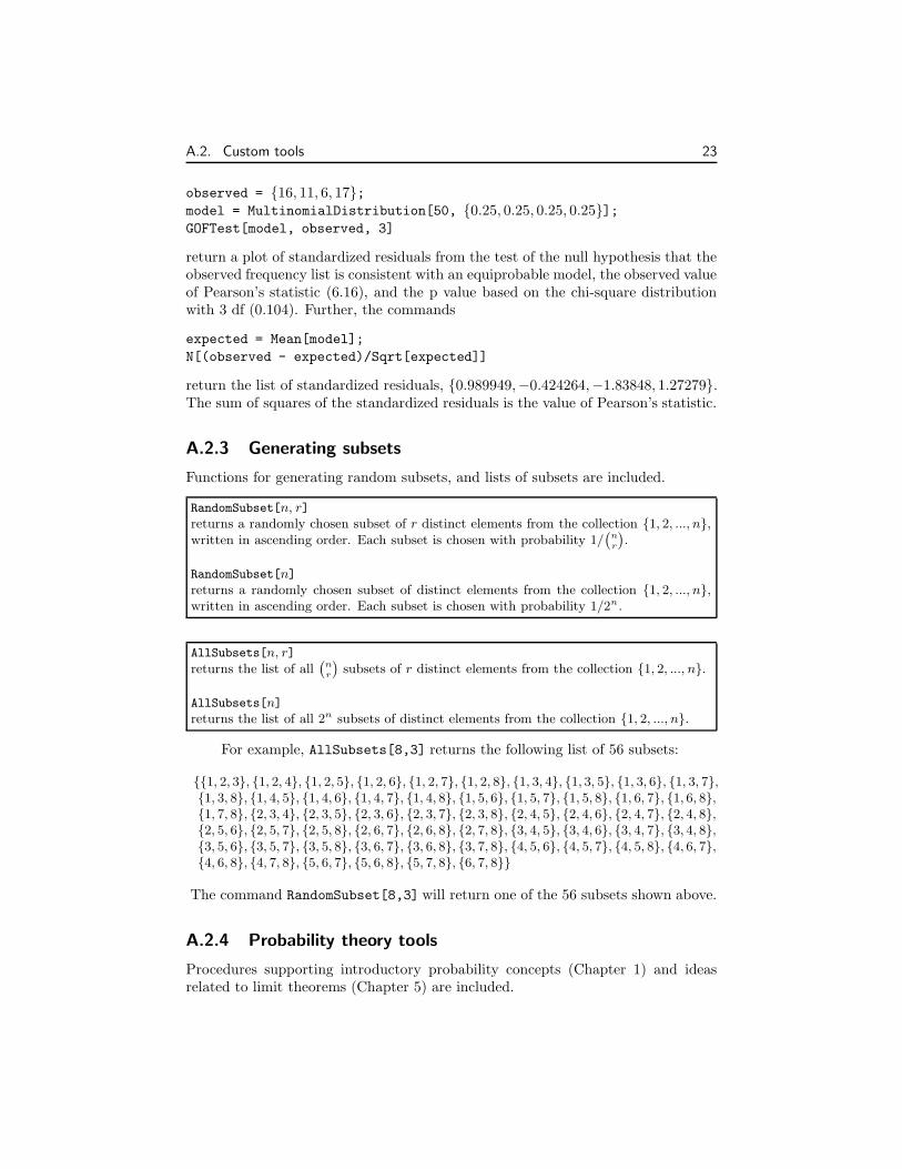
For example, AllSubsets[8,3] returns the following list of 56 subsets:
{{1, 2, 3}, {1, 2, 4}, {1, 2, 5}, {1, 2, 6}, {1, 2, 7}, {1, 2, 8}, {1, 3, 4}, {1, 3, 5}, {1, 3, 6}, {1, 3, 7},{1, 3, 8}, {1, 4, 5}, {1, 4, 6}, {1, 4, 7}, {1, 4, 8}, {1, 5, 6}, {1, 5, 7}, {1, 5, 8}, {1, 6, 7}, {1, 6, 8},{1, 7, 8}, {2, 3, 4}, {2, 3, 5}, {2, 3, 6}, {2, 3, 7}, {2, 3, 8}, {2, 4, 5}, {2, 4, 6}, {2, 4, 7}, {2, 4, 8},{2, 5, 6}, {2, 5, 7}, {2, 5, 8}, {2, 6, 7}, {2, 6, 8}, {2, 7, 8}, {3, 4, 5}, {3, 4, 6}, {3, 4, 7}, {3, 4, 8},{3, 5, 6}, {3, 5, 7}, {3, 5, 8}, {3, 6, 7}, {3, 6, 8}, {3, 7, 8}, {4, 5, 6}, {4, 5, 7}, {4, 5, 8}, {4, 6, 7},{4, 6, 8}, {4, 7, 8}, {5, 6, 7}, {5, 6, 8}, {5, 7, 8}, {6, 7, 8}}
The command RandomSubset[8,3] will return one of the 56 subsets shown above.
A.2.4 Probability theory tools
Procedures supporting introductory probability concepts (Chapter 1) and ideasrelated to limit theorems (Chapter 5) are included.
24 Appendix A. Introduction to Mathematica Commands
Card and lottery games
RandomCardHand[n]returns a plot of a randomly chosen hand of n distinct cards from a standard deck of 52cards. Each hand is chosen with probability 1/
(52
n
).
RandomCardHand[n,CardSet→list]
returns a plot of a randomly chosen hand of n distinct cards with the cards whosenumerical values are in list highlighted. Add the option Repetitions→ r to repeat theexperiment “choose n cards and record the number of cards in list” r times and returnthe results.
RandomCardHand[]
returns a plot of the numerical values of each card in a standard deck.
RandomLotteryGame[nn,n]returns the results of a random state lottery game: (1) the state randomly chooses asubset of n distinct numbers from the collection {1, 2, ..., nn} (shown as vertical lines);(2) the player randomly chooses a subset of n distinct numbers from the same collection(shown as black dots for numbers matching the state’s picks, and red dots otherwise).Each choice of subset is equally likely.
RandomLotteryGame[nn,n,Repetitions→ r]repeats the experiment “play the game and record the number of matches” r times andreturns the list of results.
Simple urn model
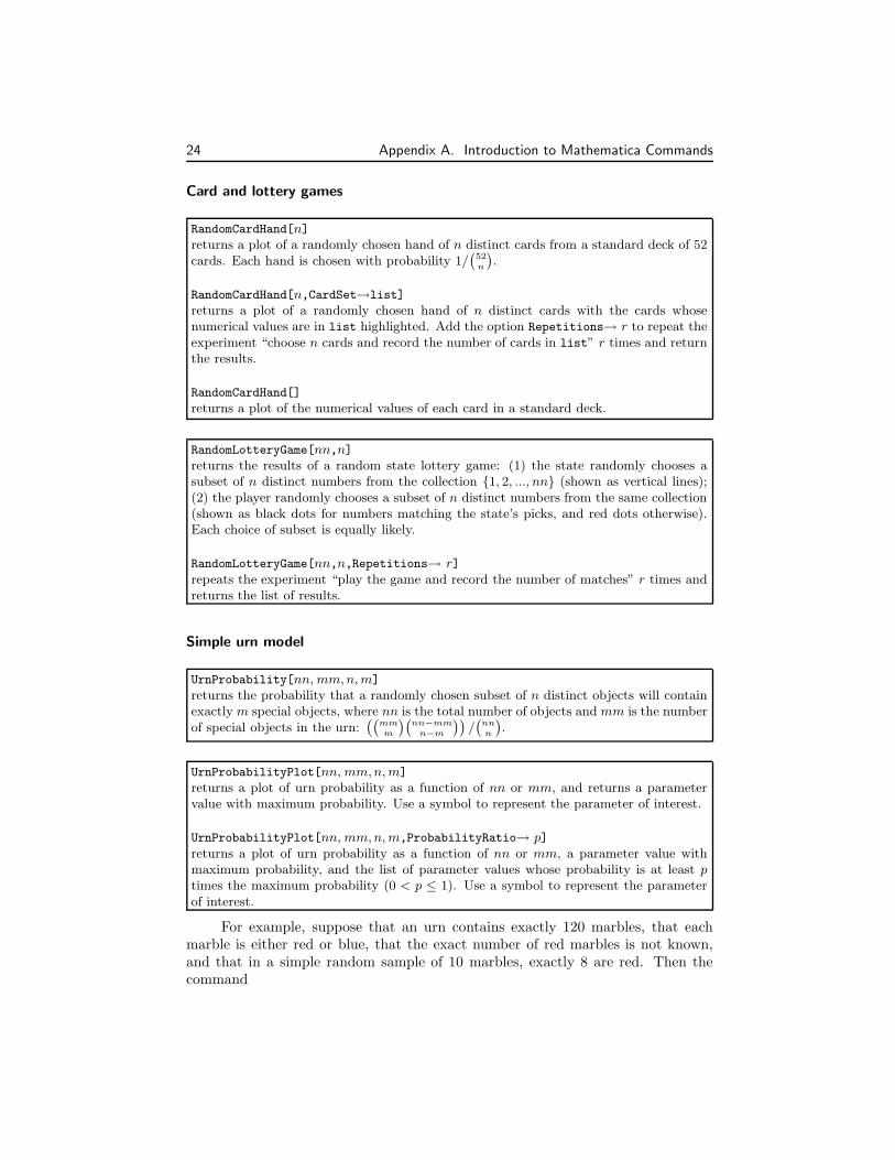
UrnProbability[nn, mm,n, m]
returns the probability that a randomly chosen subset of n distinct objects will containexactly m special objects, where nn is the total number of objects and mm is the numberof special objects in the urn:
((mm
m
)(nn−mm
n−m
))/(
nn
n
).
UrnProbabilityPlot[nn, mm,n, m]
returns a plot of urn probability as a function of nn or mm, and returns a parametervalue with maximum probability. Use a symbol to represent the parameter of interest.
UrnProbabilityPlot[nn, mm,n, m,ProbabilityRatio→ p]returns a plot of urn probability as a function of nn or mm, a parameter value withmaximum probability, and the list of parameter values whose probability is at least ptimes the maximum probability (0 < p ≤ 1). Use a symbol to represent the parameterof interest.
For example, suppose that an urn contains exactly 120 marbles, that eachmarble is either red or blue, that the exact number of red marbles is not known,and that in a simple random sample of 10 marbles, exactly 8 are red. Then thecommand

A.2. Custom tools 25
Clear[mm];
UrnProbabilityPlot[120,mm,10,8,ProbabilityRatio→0.25]
returns a plot of urn probabilities as a function of the unknown total number ofred marbles (mm), a report identifying 96 as the most likely number of red marbles,the urn probability when mm=96 (0.315314), and a list of estimates of mm with urnprobabilities at least 0.25× 0.315314 (the list is 68, 69, . . . , 113).
Sequences of running sums and averages
RandomSumPath[model,n]generates a random sample of size n from the univariate model distribution and returnsa line plot of running sums, along with the value of the nth sum.
RandomAveragePath[model,n]generates a random sample of size n from the univariate model distribution and returnsa line plot of running averages, along with the value of the nth average.
RandomWalk2D[{pNE , pNW , pSE, pSW},n]returns a plot of a random walk of n steps in the plane beginning at the origin, along withthe final position. The walk goes northeast one step with probability pNE , northwestwith probability pNW , southeast with probability pSE, and southwest with probabilitypSW .
RandomWalk2D[{pNE , pNW , pSE, pSW},n,Repetitions→ r]returns a list of r final positions of random walks of n steps beginning at the origin.
A.2.5 Statistics theory tools
Procedures supporting estimation theory concepts (Chapter 7) and hypothesis test-ing theory concepts (Chapter 8) are included.
Maximum likelihood estimation
The LikelihoodPlot function allows you to visualize ML estimation in specificsituations, as described below.
LikelihoodPlot[model,data]
returns a plot of the likelihood function for the given single-parameter model and data.Use a symbol to represent the parameter to be estimated.
LikelihoodPlot[]
returns the list of allowed models and parameters.
For example, the commands
sample={5.51, 0.05, 1.57, 4.72, 4.09, 2.40, 6.90, 5.37, 3.15, 3.87};Clear[σ];LikelihoodPlot[NormalDistribution[3,σ],sample]
26 Appendix A. Introduction to Mathematica Commands
return a normal likelihood plot for the sample data and the ML estimate of σ2,4.31603. The computations assume that the sample data are the values of a randomsample from a normal distribution with µ = 3.
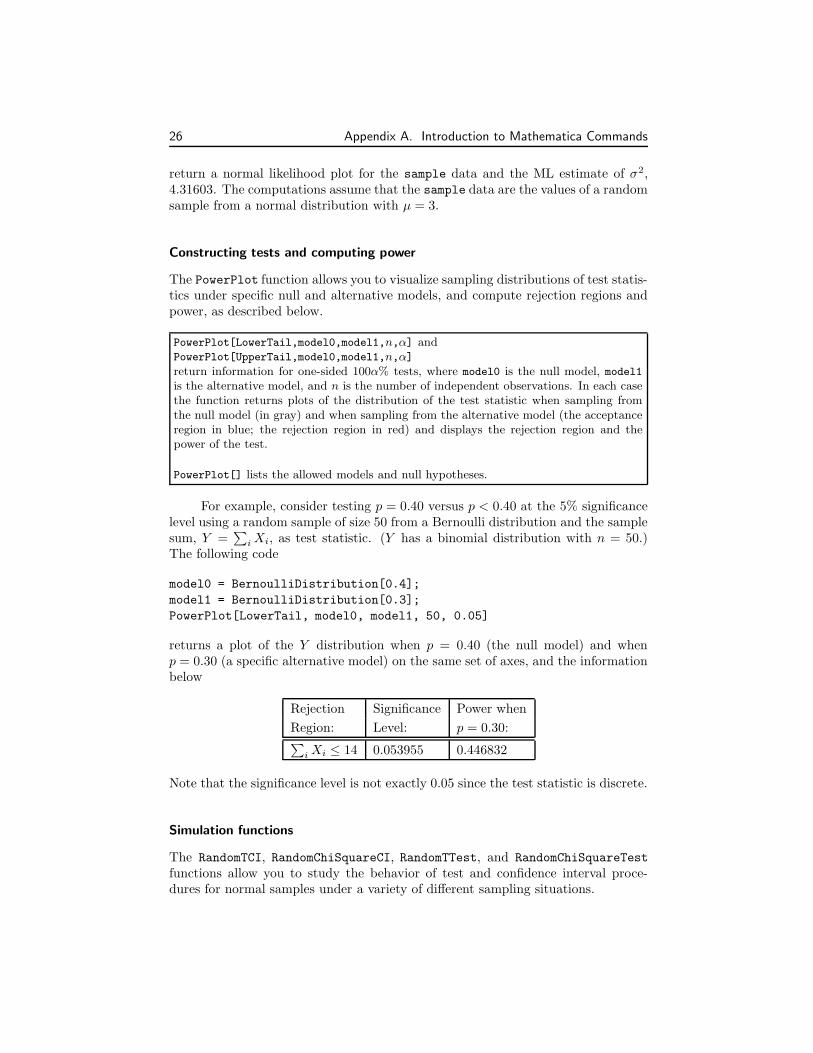
Constructing tests and computing power
The PowerPlot function allows you to visualize sampling distributions of test statis-tics under specific null and alternative models, and compute rejection regions andpower, as described below.
PowerPlot[LowerTail,model0,model1,n,α] andPowerPlot[UpperTail,model0,model1,n,α]return information for one-sided 100α% tests, where model0 is the null model, model1is the alternative model, and n is the number of independent observations. In each casethe function returns plots of the distribution of the test statistic when sampling fromthe null model (in gray) and when sampling from the alternative model (the acceptanceregion in blue; the rejection region in red) and displays the rejection region and thepower of the test.
PowerPlot[] lists the allowed models and null hypotheses.
For example, consider testing p = 0.40 versus p < 0.40 at the 5% significancelevel using a random sample of size 50 from a Bernoulli distribution and the samplesum, Y =
∑i Xi, as test statistic. (Y has a binomial distribution with n = 50.)
The following code
model0 = BernoulliDistribution[0.4];
model1 = BernoulliDistribution[0.3];
PowerPlot[LowerTail, model0, model1, 50, 0.05]
returns a plot of the Y distribution when p = 0.40 (the null model) and whenp = 0.30 (a specific alternative model) on the same set of axes, and the informationbelow
Rejection Significance Power when
Region: Level: p = 0.30:∑
i Xi ≤ 14 0.053955 0.446832
Note that the significance level is not exactly 0.05 since the test statistic is discrete.
Simulation functions
The RandomTCI, RandomChiSquareCI, RandomTTest, and RandomChiSquareTest
functions allow you to study the behavior of test and confidence interval proce-dures for normal samples under a variety of different sampling situations.
A.2. Custom tools 27
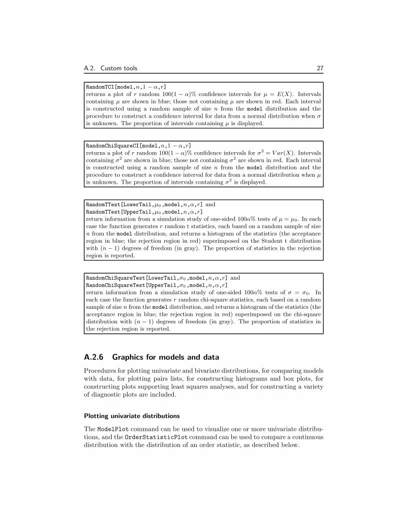
RandomTCI[model,n,1 − α,r]returns a plot of r random 100(1 − α)% confidence intervals for µ = E(X). Intervalscontaining µ are shown in blue; those not containing µ are shown in red. Each intervalis constructed using a random sample of size n from the model distribution and theprocedure to construct a confidence interval for data from a normal distribution when σis unknown. The proportion of intervals containing µ is displayed.
RandomChiSquareCI[model,n,1 − α,r]returns a plot of r random 100(1 −α)% confidence intervals for σ2 = V ar(X). Intervalscontaining σ2 are shown in blue; those not containing σ2 are shown in red. Each intervalis constructed using a random sample of size n from the model distribution and theprocedure to construct a confidence interval for data from a normal distribution when µis unknown. The proportion of intervals containing σ2 is displayed.
RandomTTest[LowerTail,µ0,model,n,α,r] andRandomTTest[UpperTail,µ0,model,n,α,r]return information from a simulation study of one-sided 100α% tests of µ = µ0. In eachcase the function generates r random t statistics, each based on a random sample of sizen from the model distribution, and returns a histogram of the statistics (the acceptanceregion in blue; the rejection region in red) superimposed on the Student t distributionwith (n − 1) degrees of freedom (in gray). The proportion of statistics in the rejectionregion is reported.
RandomChiSquareTest[LowerTail,σ0,model,n,α,r] andRandomChiSquareTest[UpperTail,σ0,model,n,α,r]return information from a simulation study of one-sided 100α% tests of σ = σ0. Ineach case the function generates r random chi-square statistics, each based on a randomsample of size n from the model distribution, and returns a histogram of the statistics (theacceptance region in blue; the rejection region in red) superimposed on the chi-squaredistribution with (n − 1) degrees of freedom (in gray). The proportion of statistics inthe rejection region is reported.
A.2.6 Graphics for models and data
Procedures for plotting univariate and bivariate distributions, for comparing modelswith data, for plotting pairs lists, for constructing histograms and box plots, forconstructing plots supporting least squares analyses, and for constructing a varietyof diagnostic plots are included.
Plotting univariate distributions
The ModelPlot command can be used to visualize one or more univariate distribu-tions, and the OrderStatisticPlot command can be used to compare a continuousdistribution with the distribution of an order statistic, as described below.
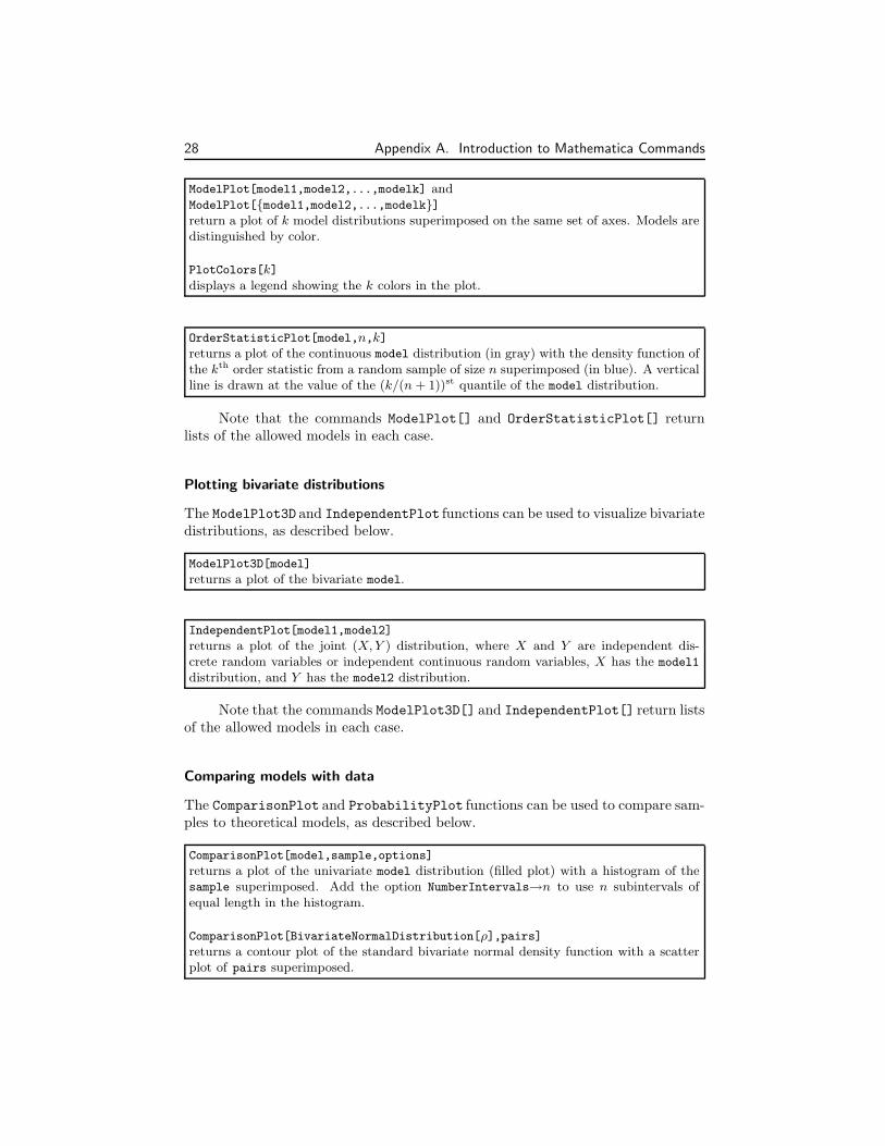
28 Appendix A. Introduction to Mathematica Commands
ModelPlot[model1,model2,...,modelk] andModelPlot[{model1,model2,...,modelk}]return a plot of k model distributions superimposed on the same set of axes. Models aredistinguished by color.
PlotColors[k]displays a legend showing the k colors in the plot.
OrderStatisticPlot[model,n,k]returns a plot of the continuous model distribution (in gray) with the density function ofthe kth order statistic from a random sample of size n superimposed (in blue). A verticalline is drawn at the value of the (k/(n + 1))st quantile of the model distribution.
Note that the commands ModelPlot[] and OrderStatisticPlot[] returnlists of the allowed models in each case.
Plotting bivariate distributions
The ModelPlot3D and IndependentPlot functions can be used to visualize bivariatedistributions, as described below.
ModelPlot3D[model]
returns a plot of the bivariate model.
IndependentPlot[model1,model2]
returns a plot of the joint (X, Y ) distribution, where X and Y are independent dis-crete random variables or independent continuous random variables, X has the model1
distribution, and Y has the model2 distribution.
Note that the commands ModelPlot3D[] and IndependentPlot[] return listsof the allowed models in each case.
Comparing models with data
The ComparisonPlot and ProbabilityPlot functions can be used to compare sam-ples to theoretical models, as described below.
ComparisonPlot[model,sample,options]
returns a plot of the univariate model distribution (filled plot) with a histogram of thesample superimposed. Add the option NumberIntervals→n to use n subintervals ofequal length in the histogram.
ComparisonPlot[BivariateNormalDistribution[ρ],pairs]returns a contour plot of the standard bivariate normal density function with a scatterplot of pairs superimposed.

A.2. Custom tools 29
ProbabilityPlot[model,sample]
returns a probability plot of sample quantiles (vertical axis) against model quantiles(horizontal axis) of the continuous model. Add the option SimulationBands→True toadd bands showing the minimum and maximum values for order statistics in 100 randomsamples of size Length[sample] from the model distribution.
Note that the commands ComparisonPlot[] and ProbabilityPlot[] returnlists of the allowed models in each case.
Plotting pairs lists, and lists of triples
The ScatterPlot command is a multi-purpose function designed to produce singleand multiple list plots, as described below.
ScatterPlot[pairs1,pairs2,. . .,pairsk,options] andScatterPlot[{pairs1, pairs2, ..., pairsk},options]return a multiple list plot of k lists of pairs using PlotColors[k] to distinguish thesamples.
ScatterPlot[{{x1 , y1, z1}, {x2, y2, z2}, . . .},options]returns a list plot of {{x1, y1}, {x2, y2}, . . .} using color to distinguish the unique z-values.
ScatterPlot[]
returns a list of the allowed options.
The options include adding axes and plot labels, producing line plots (wheresuccessive pairs are joined by line segments), adding a least squares fit line and dis-playing the sample correlation (for a single list of pairs), and visualizing permutationand bootstrap methods (for a single list of pairs).
Constructing histograms and box plots
The SamplePlot command is used to construct an empirical histogram of sampledata (or several histograms on the same set of axes), and the BoxPlot command isused to construct side-by-side box plots of sample data, as described below.
SamplePlot[list1,list2,..,listk],options andSamplePlot[{list1,list2,...,listk},options]return a plot of k empirical histograms superimposed on the same set of axes usingPlotColors[k] to distinguish the samples. Labels may be added to the plot. Add theoption NumberIntervals→n to use n subintervals of equal length in each histogram.
BoxPlot[list1,list2,...,listk,options] andBoxPlot[{list1,list2,...,listk},options]return a plot of k side-by-side box plots. Labels may be added to the plot.
Plots supporting least squares analyses
The SmoothPlot and PartialPlot functions support least squares analyses (Chap-ter 14). The SmoothPlot command returns a scatter plot of one or more lists of
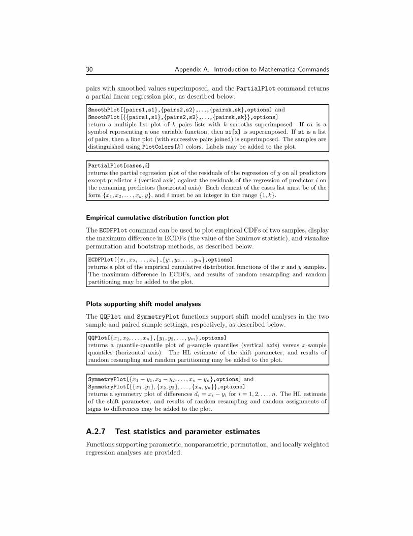
30 Appendix A. Introduction to Mathematica Commands
pairs with smoothed values superimposed, and the PartialPlot command returnsa partial linear regression plot, as described below.
SmoothPlot[{pairs1,s1},{pairs2,s2},. . .,{pairsk,sk},options] andSmoothPlot[{{pairs1,s1},{pairs2,s2},. . .,{pairsk,sk}},options]return a multiple list plot of k pairs lists with k smooths superimposed. If si is asymbol representing a one variable function, then si[x] is superimposed. If si is a listof pairs, then a line plot (with successive pairs joined) is superimposed. The samples aredistinguished using PlotColors[k] colors. Labels may be added to the plot.
PartialPlot[cases,i]returns the partial regression plot of the residuals of the regression of y on all predictorsexcept predictor i (vertical axis) against the residuals of the regression of predictor i onthe remaining predictors (horizontal axis). Each element of the cases list must be of theform {x1, x2, . . . , xk, y}, and i must be an integer in the range {1, k}.
Empirical cumulative distribution function plot
The ECDFPlot command can be used to plot empirical CDFs of two samples, displaythe maximum difference in ECDFs (the value of the Smirnov statistic), and visualizepermutation and bootstrap methods, as described below.
ECDFPlot[{x1, x2, . . . , xn},{y1, y2, . . . , ym},options]returns a plot of the empirical cumulative distribution functions of the x and y samples.The maximum difference in ECDFs, and results of random resampling and randompartitioning may be added to the plot.
Plots supporting shift model analyses
The QQPlot and SymmetryPlot functions support shift model analyses in the twosample and paired sample settings, respectively, as described below.
QQPlot[{x1, x2, . . . , xn},{y1, y2, . . . , ym},options]returns a quantile-quantile plot of y-sample quantiles (vertical axis) versus x-samplequantiles (horizontal axis). The HL estimate of the shift parameter, and results ofrandom resampling and random partitioning may be added to the plot.
SymmetryPlot[{x1 − y1, x2 − y2, . . . , xn − yn},options] andSymmetryPlot[{{x1 , y1}, {x2, y2}, . . . , {xn, yn}},options]returns a symmetry plot of differences di = xi − yi for i = 1, 2, . . . , n. The HL estimateof the shift parameter, and results of random resampling and random assignments ofsigns to differences may be added to the plot.
A.2.7 Test statistics and parameter estimates
Functions supporting parametric, nonparametric, permutation, and locally weightedregression analyses are provided.

A.2. Custom tools 31
Pooled t and Welch t statistics
PooledTStatistic[{x1 , x2, . . .}, {y1, y2, . . .},δ0]
returns the pooled t statistic for the test of the null hypothesis E(X) − E(Y ) = δ0.
WelchTStatistic[{x1 , x2, . . .}, {y1, y2, . . .},δ0]
returns the Welch t statistic for the test of the null hypothesis E(X) − E(Y ) = δ0.
Sample correlation and rank correlation statistics
Correlation[{x1 , x2, . . . , xn}, {y1, y2, . . . , yn}] andCorrelation[{{x1 , y1}, {x2, y2}, . . .}]return the sample correlation coefficient.
RankCorrelation[{x1 , x2, . . . , xn}, {y1, y2, . . . , yn}] andRankCorrelation[{{x1 , y1}, {x2, y2}, . . .}]return the value of Spearman’s rank correlation coefficient.
Note that each function allows two types of input: either separate lists of x-and y- coordinates, or a list of (x, y) pairs.
Statistics for one or more samples
RankSumStatistic[{x1 , x2, . . . , xn}, {y1, y2, . . . , ym}]returns the value of Wilcoxon’s rank sum statistic for the first sample, R1.
SignedRankStatistic[{x1 − y1, x2 − y2, . . .}] andSignedRankStatistic[{{x1 , y1}, {x2, y2}, . . .}]return the value of Wilcoxon’s signed-rank statistic, W+.
SmirnovStatistic[{x1 , x2, . . .}, {y1, y2, . . .}]returns the maximum absolute difference between the empirical cumulative distributionfunctions for the x and y lists.
TrendStatistic[{x1 , x2, . . . xn}]returns the value of Mann’s trend statistic.
KruskalWallisStatistic[{sample1,sample2,. . .,sampleI}]returns the value of the Kruskal-Wallis statistic for the list of samples, where each sampleis a list of two or more numbers.
FriedmanStatistic[{sample1,sample2,. . .,sampleI}]returns the value of the Friedman statistic, where the input is a matrix of real numbers.The number of samples, and the common number of observations in each sample, mustbe at least 2.
32 Appendix A. Introduction to Mathematica Commands
Shift parameter estimation
The HodgesLehmannDelta function can be used to compute the HL estimate of theshift parameter in two sample and paired sample analyses, as described below.
HodgesLehmannDelta[sample1,sample2]
returns the HL estimate of ∆=Median(X)−Median(Y ) for independent samples.
HodgesLehmannDelta[{x1 − y1, x2 − y2, . . .}] andHodgesLehmannDelta[{{x1 , y1}, {x2, y2}, . . .}]return the HL estimate of ∆=Median(X − Y ) for paired samples.
Locally weighted regression estimation
The LowessSmooth function can be used to approximate the conditional expectationof Y given X for fixed values of X , as described below.
LowessSmooth[{{x1 , y1}, {x2, y2}, . . .},p]returns a list of pairs of the form (unique x-value, smoothed y-value) using a lowesssmooth with 100p% of the data included at each point.
LowessSmooth[{{x1 , y1}, {x2, y2}, . . .},p,x0]
returns the smoothed y-value when x = x0.
The LowessSmooth function implements Cleveland’s locally weighted regres-sion method using tricube weights. The robustness step is omitted. The algorithmis described in the book by Chambers, Cleveland, Kleiner, and Tukey (WadsworthInternational Group, 1983, page 121). (See Section 14.4.)
A.2.8 Methods for quantiles and proportions
Functions for computing sample quantiles and quantile confidence intervals usingthe methods discussed in Chapter 9, and for constructing confidence intervals forthe probability of success in Bernoulli/binomial experiments are included. In eachconfidence interval procedure, if the confidence level option is omitted, then a 95%confidence interval is returned.
Estimating quantiles
SampleQuantile[{x1 , x2, . . . , xn},p]returns the pth sample quantile, where 1/(n + 1) ≤ p ≤ n/(n + 1).
SampleQuartiles[{x1 , x2, . . . , xn}]returns the sample 25th, 50th, and 75th percentiles, where n ≥ 3.
SampleInterquartileRange[{x1 , x2, . . . , xn}]returns the sample interquartile range, where n ≥ 3.
A.2. Custom tools 33
QuantileCI[{x1 , x2, . . . , xn},p,ConfidenceLevel→ 1 − α]returns a 100(1 − α)% confidence interval for the pth model quantile.
Estimating Bernoulli/binomial probability of success
BinomialCI[x,n,ConfidenceLevel→ 1 − α]returns the 100(1−α)% confidence interval for the binomial success probability p basedon inverting hypothesis tests, where x is the number of successes in n trials (0 ≤ x ≤ n).The maximum number of iterations used to search for the endpoints is set at 50; toincrease this limit, add the option MaxIterations→m (for some m).
A.2.9 Rank-based methods
Functions for (1) computing ranks and signed ranks, (2) conducting rank sum,signed rank, rank correlation, trend, Kruskal-Wallis, and Friedman tests, and (3)constructing confidence intervals for the shift parameter in two sample and pairedsample settings are provided. Each test and confidence interval procedure takes tiesinto account. (Reference: Lehmann, Holden-Day, Inc., 1975.)
Computing ranks and signed ranks
Ranks[{x1, x2, . . .}]returns a list of ranks for the single sample.
Ranks[{{x1 , x2, . . .}, {y1, y2, . . .}, . . .}]returns a list of lists of ranks for each sample in the combined sample.
SignedRanks[{x1 − y1, x2 − y2, . . .}] andSignedRanks[{{x1 , y1}, {x2, y2}, . . .}]return the list of signed ranks for the sample of differences {x1 − y1, x2 − y2, . . .}.
For example, if samples is the following list of two samples,
{{104.6, 82.5, 66.8, 113.4, 135.6, 122.4}, {93.6, 110.2, 74.8, 81.8}}
then Ranks[samples] returns {{6, 4, 1, 8, 10, 9}, {5, 7, 2, 3}}.
Rank sum and signed rank tests
RankSumTest[{x1 , x2, . . . , xn}, {y1, y2, . . . , ym},options]returns the results of a one sided rank sum test using R1 as test statistic.
SignedRankTest[{x1 − y1, x2 − y2, . . .},options] andSignedRankTest[{{x1 , y1}, {x2, y2}, . . .},options]returns the results of a one-sided Wilcoxon signed rank test using W+ as test statistic.
34 Appendix A. Introduction to Mathematica Commands
In each case, p values are computed using the normal approximation to thesampling distribution of the test statistic; to use the exact sampling distribution,add the option ExactDistribution→True. The exact distribution should be usedwhen sample sizes are small.
To conduct a two sided test, add the option TwoSided→True. For additionaloptions, evaluate the commands ?RankSumTest and ?SignedRankTest.
Rank correlation test
RankCorrelationTest[{x1 , x2, . . . , xn}, {y1, y2, . . . , yn},options] andRankCorrelationTest[{{x1 , y1}, {x2, y2}, . . .},options]return the results of a one sided test of randomness using the Spearman rank correlationcoefficient as test statistic.
P values are computed using the normal approximation to the sampling dis-tribution of the rank correlation statistic. To conduct a two sided test, add theoption TwoSided→True.
Trend test
TrendTest[{x1 , x2, . . . , xn},options]returns the results of a one sided test of randomness using Mann’s trend statistic.
P values for the trend test are computed using the normal approximation tothe sampling distribution of the test statistic; to use the exact sampling distribution,add the option ExactDistribution→True. The exact distribution should be usedwhen sample sizes are small.
To conduct a two sided test, add the option TwoSided→True.
Kruskal-Wallis and Friedman tests
KruskalWallisTest[{sample1,sample2,. . .,sampleI}]returns results of a Kruskal-Wallis test for the list of samples, where each sample is alist of two or more numbers.
FriedmanTest[{sample1,sample2,. . .,sampleI}]returns results of a Friedman test, where the input is a matrix of real numbers. Thenumber of samples, and the common number of observations in each sample, must be atleast 2.
In each case, p values are computed using the chi-square approximation to thesampling distribution of the test statistic.
Confidence interval procedures for shift parameters
RankSumCI[{x1 , x2, . . . , xn}, {y1, y2, . . . , ym},ConfidenceLevel→ 1 − α]returns a 100(1 − α)% confidence interval for Median(X)−Median(Y ).
A.2. Custom tools 35
SignedRankCI[{x1 − y1, x2 − y2, . . .},ConfidenceLevel→ 1 − α] andSignedRankCI[{{x1 , y1}, {x2, y2}, . . .},ConfidenceLevel→ 1 − α]returns a 100(1 − α)% confidence interval for Median(X − Y ).
In each case, confidence intervals are computed using the normal approxima-tion to the sampling distribution of the statistics; to use the exact sampling distri-bution, add the option ExactDistribution→True. The exact distribution shouldbe used when sample sizes are small. If the confidence level option is omitted, thena 95% confidence interval is returned.
A.2.10 Permutation methods
Functions for computing random reorderings, and permutation confidence intervalsfor the slope in a simple linear model are provided. The confidence interval methodis discussed in the book by Maritz (Chapman & Hall, 1995, page 120).
Random reordering of sample data
RandomPartition[{sample1,sample2,. . .,samplek}]returns a random partition of the objects in
Flatten[{sample1,sample2,. . .,samplek},1]
into lists of lengths n1=Length[sample1], . . ., nk=Length[samplek], respectively. Thechoice of each partition is equally likely.
RandomPermutation[sample]
returns a random permutation of the objects in the sample list. The choice of eachpermutation is equally likely.
RandomSign[{x1 , x2, . . .}]returns a list of numbers whose kth term is either +xk or −xk. Each list is chosen withprobability 1/2m, where m is the number of non-zero elements in {x1, x2, . . .}.
For example, if samples is the following list of 3 lists:
{{a, b, c, d}, {e, f, g}, {h, i, j, k, `}}
then RandomPartition[samples] could return any one of the Multinomial[4,3,5]= 27720 partitions of the objects a, b, . . . , ` into sublists of lengths 4, 3, 5. Onepossibility is
{{k, `, i, c}, {g, a, j}, {f, h, b, d, e}}.
Permutation confidence interval for slope
SlopeCI[pairs, ConfidenceLevel→ 1 − α, RandomPermutations→ r]returns an approximate 100(1−α)% permutation confidence interval for the slope basedon r random permutations, where pairs is a list of pairs of numbers.
36 Appendix A. Introduction to Mathematica Commands
For example, if
pairs={{19.53, −115.42}, {12.17, −106.79}, {13.75, −47.13}, {0.92, 36.09}, {11.71, 33.95},
{4.33, 24.06}, {5.74, 6.59}, {19.81,−93.56}, {3.06, 8.26}, {11.00, −29.24}};
is the list of data pairs, then the command Fit[pairs,{1,x},x] returns the linearleast squares fit formula, 47.2251− 7.40484 x, and the command
SlopeCI[pairs, RandomPermutations→2000]
returns an approximate 95% confidence interval for the slope based on 2000 randompermutations. A possible result is [−11.441,−3.09877].
A.2.11 Bootstrap methods
Functions for computing random resamples, summarizing bootstrap results, andconstructing approximate bootstrap confidence intervals using Efron’s improvedprocedure (the BCa method) in the nonparametric case are provided. The confi-dence interval procedure is discussed in the book by Efron and Tibshirani (Chapman& Hall, 1993, page 184).
Random resample of sample data
RandomResample[sample]
returns a random sample of size Length[sample] from the observed distribution of thesample data.
Note that a random resample is not the same as a random permutation of thesample data. In a random resample, observations are chosen with replacement fromthe original sample list.
Summarizing bootstrap estimation results
The BootstrapSummary command returns a histogram of estimated errors super-imposed on the normal distribution with the same mean and standard deviation,estimates of bias and standard error, and simple approximate confidence intervals(Section 12.2), as described below.
BootstrapSummary[results,observed,ConfidenceLevel→ 1 − α]returns a summary of results from a bootstrap analysis, where observed is the observedvalue of the scalar parameter of interest. The summary includes simple 100(1 − α)%confidence intervals for the parameter of interest.
The BootstrapSummary function is appropriate for summarizing the resultsof both parametric and nonparametric bootstrap analyses.
A.2. Custom tools 37
Improved bootstrap confidence intervals
BootstrapCI1[sample,f, ConfidenceLevel→ 1 − α,RandomResamples→ r]
returns a 100(1−α)% bootstrap confidence interval for a parameter θ based on r randomresamples from sample. The symbol f represents a real-valued function of one variableused to estimate θ from a sample list.
BootstrapCI2[{sample1,sample2,. . .},f, ConfidenceLevel→ 1 − α,RandomResamples→ r]
returns a 100(1−α)% bootstrap confidence interval for a parameter θ based on r randomresamples from each sample in the list. The symbol f represents a real-valued functionof one variable (a list of sample lists) used to estimate θ.
In each case, if the confidence level option is omitted, then a 95% confidenceinterval is returned. If the random resamples option is omitted, then 1000 randomresamples are used.
A.2.12 Analysis of variance methods
Functions for one-way layouts, blocked designs, and balanced two-way layouts, andfor Bonferroni analyses are provided. (See Chapter 13.)
One-way layout
AnovaOneWay[{sample1,sample2,...,sampleI}]returns analysis of variance results for the one-way layout, where each sample is a list of2 or more numbers. The output includes an analysis of variance table and a line plot ofestimated group means.
BonferroniOneWay[{sample1,sample2,...,sampleI},α]returns results of a Bonferroni analysis for the one-way layout, where each sample is a listof 2 or more numbers. The overall significance level is at most α. The output includes thetotal number of comparisons, the rejection region for each test, the appropriate samplingdistribution for the test statistics, and a list of significant mean differences.
Note that an estimated difference in means, say µi − µk, is included in theoutput list of the Bonferroni analysis if the two sided pooled t test of µi = µk isrejected at the α/m level, where m =
(I2
).
Blocked design
AnovaBlocked[{sample1,sample2,...,sampleI}]returns results of analysis of variance for the blocked design, where the input is a matrixof real numbers. The number of samples, and the common number of observations ineach sample, must be at least 2. The output includes an analysis of variance table anda line plot of estimated group effects.
38 Appendix A. Introduction to Mathematica Commands
BonferroniBlocked[{sample1,sample2,...,sampleI},α]returns results of a Bonferroni analysis for the blocked design, where the input is a matrixof real numbers. The number of samples, and the common number of observationsin each sample, must be at least 2. The overall significance level is at most α. Theoutput includes the total number of comparisons, the rejection region for each test, theappropriate sampling distribution for the test statistics, and a list of significant meandifferences.
Note that an estimated difference in means, say µi. − µk., is included in theoutput list of the Bonferroni analysis if the two sided paired t test of µi. = µk. isrejected at the α/m level, where m =
(I2
).
Balanced two-way layout
AnovaTwoWay[{row1,row2,...,rowI}]returns results of analysis of variance for the balanced two-way layout, where the inputis a matrix of samples of equal lengths. The number of rows, the number of columns,and the common number of observations per sample must each be at least 2. The outputincludes an analysis of variance table and line plots of estimated group means by row,using PlotColors[I] to distinguish the plots.
A.2.13 Contingency table methods
Functions for analyzing I-by-J frequency tables, generating random tables for per-mutation analyses, analyzing the odds ratio in fourfold tables, Fisher’s exact test,and McNemar’s test are provided. (See Chapter 15.)
Analysis of two-way tables
The function TwoWayTable is a general routine for analyzing I-by-J frequency ta-bles using Pearson’s statistic, the Kruskal-Wallis statistic, or the Spearman rankcorrelation statistic, as described below.
TwoWayTable[table]
returns results of an analysis of independence of row and column factors, or of homo-geneity of row or column models, using Pearson’s chi-square test. The output includesa table of standardized residuals.
TwoWayTable[table,Method→MeanTable]
returns a table of estimated cell expectations for tests of independence of row and columnfactors, or of homogeneity of row or column models.
TwoWayTable[table,Method→KruskalWallis]
returns results of a Kruskal-Wallis test of equality of row distributions.
TwoWayTable[table,Method→RankCorrelation,options]
returns results of a one sided test of independence of row and column distributions; fora two sided test, add the option TwoSided→True.
A.2. Custom tools 39
Note that the chi-square approximation to the sampling distribution of Pear-son’s statistic is adequate when all estimated cell expectations are 5.0 or more. Fortables with small cell expectations, a permutation analysis can be done.
Generating random tables
RandomTable[table]
returns a random two-way frequency table with the same row and column totals as tablebased on the general permutation strategy.
Odds ratio analyses in fourfold tables
The OddsRatioCI function returns a large sample approximate confidence intervalfor the odds ratio based on the normal approximation to the sampling distribution oflog(OR); use the ExactMethod→True option to construct an interval when samplesizes are small (Section 15.4). If the confidence level option is omitted, then a 95%confidence interval is returned. The small sample method is discussed in the bookby Agresti (John Wiley & Sons, 1990, page 67).
OddsRatioCI[{{x11 , x12}, {x21, x22}}, ConfidenceLevel→ 1 − α]returns an approximate 100(1 − α)% confidence interval for the odds ratio. All cellfrequencies must be positive.
OddsRatioCI[{{x11 , x12}, {x21, x22}},ConfidenceLevel→ 1 − α,ExactMethod→True]
returns a 100(1 − α)% confidence interval for the odds ratio based on inverting hypoth-esis tests. All cell frequencies must be positive. The maximum number of iterationsused to search for the endpoints is set at 50; to increase this limit, add the optionMaxIterations→m.
Tests for fourfold tables
FisherExactTest[{{x11 , x12}, {x21, x22}}]returns results of the two sided Fisher exact test.
McNemarTest[{{x11 , x12}, {x21, x22}}]returns exact and approximate results of McNemar’s test for paired samples.

40 Appendix A. Introduction to Mathematica Commands
Index
! (factorial function), 3!= (not equal), 4′ (derivative), 14( ) (for subexpressions), 2∗ (multiply), 2+ (add), 2− (subtract), 2/ (divide), 2< (less than), 4<= (less than or equal to), 4== (equal), 4> (greater than), 4>= (greater than or equal to), 4→ (for rules), 15|| (logical or), 4∧ (power function), 2{ } (for lists), 7. (dot product), 11, 12/. (replace all function), 15:= (delayed assignment), 5; (result not returned), 5= (immediate assignment), 5? (for online help), 2, 21@@ (apply function), 11[[ ]] (list part), 9, 11[ ] (for function arguments), 5# (in unnamed function), 9& (in unnamed function), 9&& (logical and), 4(for patterns), 5
absolute value function, 3AllSubsets function, 23And function, 4AnovaBlocked function, 37AnovaOneWay function, 37AnovaTwoWay function, 38
antiderivative function, 14Apart function, 15Append function, 8Apply function, 10arithmetic functions, 2assignment
delayed, 5immediate, 5
assumptionsin definite integrals, 14
binomial coefficient, 3BinomialCI function, 33bivariate distributions, 21BonferroniBlocked function, 38BonferroniOneWay function, 37boolean functions, 4bootstrap confidence intervals, 37BootstrapSummary function, 36BoxPlot function, 29
card games, 24case-sensitive, 4CDF function, 17Clear function, 5Coefficient function, 15colors in plots, 28Column function, 11combinations, number of, 3ComparisonPlot function, 28confidence intervals
binomial probability, 33bootstrap, 37difference in means, 18mean, 17odds ratio, 39quantiles, 33
41
42 Index
random chi-square, 27random t, 27ratio of variances, 18shift parameters, 34simple bootstrap, 36slope, 35variance, 17
constants, 2contingency tables, 38Correlation function, 22, 31Count function, 10CumulativeSums function, 8
D function, 14definite integral function, 14
assumptions, 14delayed assignment, 5Delete function, 9derivative function, 14distributions
bivariate, 21multinomial, 22univariate, 17
Dot product, 11, 12Drop function, 9
E constant, 2ECDFPlot function, 30EvenQ function, 4Expand function, 15exponential function, 3
Factor function, 15Factorial function, 3False constant, 2FilledPlot function, 13FindFit function, 19FindRoot function, 16First function, 9FisherExactTest function, 39Fit function, 19Flatten function, 12Floor function, 3Frequencies function, 10FriedmanStatistic function, 31FriedmanTest function, 34
function, 5pure, 9unnamed, 9
gamescard hands, 24state lottery, 24
GOFTest function, 22
histograms, 29HodgesLehmannDelta function, 32hypothesis tests
one-way anova, 37blocked anova, 37contingency tables, 38difference in means, 18Fisher exact test, 39Friedman test, 34goodness-of-fit, 22Kruskal-Wallis test, 34McNemar test, 39means, 18random chi-square, 27random t, 27rank correlation, 34rank sum test, 33ratio of variances, 18signed rank test, 33trend, 34two-way anova, 38variances, 18
I constant, 2If function, 6immediate assignment, 5IndependentPlot function, 28Infinity constant, 2IntegerQ function, 4Integrate function, 14Intersection function, 8Inverse function, 12inverse trigonometric functions, 3iterator, 2
Join function, 8
KruskalWallisStatistic function, 31
Index 43
KruskalWallisTest function, 34
Last function, 9least squares, 19Length function, 7LikelihoodPlot function, 25line plot, 29list plot, 29lists, 7
append function, 8count function, 10cumulative sums, 8delete from list, 9dot product, 11drop from list, 9first element, 9flatten, 12frequencies, 10intersection function, 8join function, 8last element, 9length of list, 7map function, 8maximum element, 11mean of list, 11median of list, 11membership function, 4minimum element, 11outer product, 8part of list, 9partition, 12permutations function, 8prepend function, 8product of elements, 10range counts, 10range function, 7select function, 9sort the list, 7standard deviation of list, 11standardize the list, 11sum of elements, 10table command, 7table form, 12take from list, 9trimmed mean, 11union function, 8
variance of list, 11logarithmic function, 3logical connectors, 4logical operators, 4LowessSmooth function, 32
Map function, 8matrix, 11
ith row, 11jth column, 11inverse, 12product, 12transpose, 12
Max function, 11McNemarTest function, 39Mean function, 11, 17, 22MeanCI function, 17MeanDifferenceCI function, 18MeanDifferenceTest function, 18MeanTest function, 18Median function, 11MemberQ function, 4Min function, 11ModelPlot function, 28ModelPlot3D function, 28Module command, 6multinomial coefficient, 3multinomial distribution, 22multinomial goodness-of-fit, 22multiple list plot, 29
N function, 4Negative function, 4Not function, 4NSolve function, 16numerical approximation, 4
OddQ function, 4OddsRatioCI function, 39Or function, 4OrderStatisticPlot function, 28Outer product function, 8
Part of list, 9PartialPlot function, 30Partition function, 12
44 Index
partitions, number of, 3pattern, 5PDF function, 17, 22Permutations function, 8Pi constant, 2Plot function, 13PlotColors function, 28plotting
BoxPlot, 29colors, 28ComparisonPlot, 28ECDFPlot, 30FilledPlot, 13histograms, 29IndependentPlot, 28ModelPlot, 28ModelPlot3D, 28OrderStatisticPlot, 28PartialPlot, 30Plot, 13ProbabilityPlot, 29QQPlot, 30SamplePlot, 29ScatterPlot, 29SmoothPlot, 30SymmetryPlot, 30
PooledTStatistic function, 31Positive function, 4Power function, 3PowerPlot function, 26Prepend function, 8ProbabilityPlot function, 29Product function, 2pseudo-random numbers, 3pure function, 9
QQPlot function, 30Quantile function, 17QuantileCI function, 33quantiles, sample values, 32
Random function, 3, 17, 22RandomArray function, 17, 22RandomAveragePath function, 25RandomCardHand function, 24RandomChiSquareCI function, 27
RandomChiSquareTest function, 27RandomLotteryGame function, 24RandomPartition function, 35RandomPermutation function, 35RandomResample function, 36RandomSign function, 35RandomSubset function, 23RandomSumPath function, 25RandomTable function, 39RandomTCI function, 27RandomTTest function, 27RandomWalk2D function, 25Range function, 7RangeCounts function, 10RankCorrelation function, 31RankCorrelationTest function, 34Ranks function, 33RankSumCI function, 34RankSumStatistic function, 31RankSumTest function, 33Regress function, 20Remove function, 5ReplaceAll function, 15Round function, 3rules, 15running averages, 25running sums, 25
SampleInterquartileRange function, 32SamplePlot function, 29SampleQuantile function, 32SampleQuartiles function, 32ScatterPlot function, 29Select function, 9shift parameter
confidence interval, 34estimate, 32
Sign function, 3SignedRankCI function, 35SignedRanks function, 33SignedRankStatistic function, 31SignedRankTest function, 33Simplify function, 15SlopeCI function, 35SmirnovStatistic function, 31SmoothPlot function, 30
Index 45
Solve function, 16Sort function, 7square root function, 3StandardDeviation function, 11, 17,
22Standardize function, 11state lottery game, 24structured list, 11subsets
list of all subsets, 23random subset, 23
Sum function, 2symbolic operations, 15SymmetryPlot function, 30
Table command, 7TableForm function, 12Take function, 9Together function, 15Transpose function, 12TrendStatistic function, 31TrendTest function, 34trigonometric functions, 3TrimmedMean function, 11True constant, 2TwoWayTable function, 38
Union function, 8univariate distributions, 17unnamed function, 9UrnProbability function, 24UrnProbabilityPlot function, 24
Variance function, 11, 17, 22VarianceCI function, 17VarianceRatioCI function, 18VarianceRatioTest function, 18VarianceTest function, 18
WelchTStatistic function, 31Which function, 6