1 introduction to mathematica - bilder.buecher.de file2 1 introduction to mathematica imental data...

1 Introduction to Mathematica

1.1 What is Mathematica?

Mathematica is a computer program (or, more correctly, a system of computerprograms) for performing mathematical operations such as symbolic manipulation,numerical calculations, graphics, and programming. Mathematica is sometimes de-scribed as a computer algebra system, probably in deference to the strong sym-bolic but somewhat limited numerical capabilities of its earliest versions, but ithas evolved into system that is now a very practical tool for large scale numeri-cal calculations. Its applications can range from simple calculations to complicatedprograms, and Mathematica can be a powerful tool for quantitative geoscientistssuch as geologists, geographers, geophysicists, hydrologists, and oceanographers.Because it is a general mathematics system rather than a task-specific application,however, its utility may not be apparent at first glance. It does not, after all, solvespecific geoscientific problems any more than do programming languages such asC or FORTRAN or spreadsheet programs. Over the years I have encountered manygeoscientists who know that Mathematica exists, but are not sure what it does withregard to the specific problems they face in their research or professional practice.The short answer is that it does nothing geoscientific in particular, but has the poten-tial to do just about anything that a user can imagine. Computational Geoscienceswith Mathematica is intended to help fill that gap a by illustrating how Mathematicacan be used to formulate, solve, and visualize a variety of problems of interest togeoscientists.

Mathematica was first published by Wolfram Research in 1988 and the latestversion, 5.0, was released during Summer 2003. This book was written using ver-sions of Mathematica ranging from 4.1 through 5.0, and care has been taken toensure that the examples will work with both version 5.0 and its immediate prede-cessor, version 4.2. Version 5.0 is available for Windows 98/Me/NT 4.0/2000/XPand several versions of the Unix (including Macintosh OS X) and Linux operatingsystems. Specialized versions are available for web applications, grid computingusing computer clusters or multiprocessor computers, and student use.

The functionality of Mathematica, which includes many standard packages withspecialized functions in areas such as statistics and graphics, can be expanded withpackages available through Wolfram Research, other commercial sources, or thepublic domain. Packages that may be of interest to geoscientists, but which are notcovered in this book, include a database access kit, digital image processing, exper-

2 1 Introduction to Mathematica

imental data analysis, real time 3-D graphics, fuzzy logic, neural networks, signalprocessing, time series analysis, and wavelets. Readers interested in those packagesshould contact Wolfram Research for more information about their capabilities andavailability.

1.2 Getting Help

Mathematica offers several kinds of documentation and online help. One source isThe Mathematica Book (Wolfram, 1999), the current edition of which is writtenfor version 4.0. A paper copy is included with professional (but not student) ver-sions of Mathematica. Mathematica also offers a Help menu that includes a HelpBrowser (which can access a digital copy of The Mathematica Book), a ten-minutetutorial, a hyperlink to a web information center maintained by Wolfram Research(http://library.wolfram.com/infocenter), and a hyperlink to the general Wolfram Re-search web site (http://www.wolfram.com). If you know the name of a function,typing ?function then pressing Enter will return a brief description of the functionwith a hyperlink to more information. If you only know part of the function name,typing a question mark followed at least the first letter of the function name andthen pressing Command-k will return a list of Mathematica functions that matchthe letters typed.

There are a number of good introductory books about Mathematica, in par-ticular The Beginner’s Guide to Mathematica Version 4 (Glynn and Gray, 2000).Another useful source of information is the comp.soft-sys.math.mathematica news-group, which can be accessed through http://groups.google.com. For those wishingto retain expert help, Wolfram Research maintains a list of accredited Mathematicaconsultants.

1.3 Installing and Running Mathematica

Virtually any modern personal computer or workstation should have enough mem-ory and computational speed to run Mathematica although, as with all software, themore memory and the faster the processor the better. The examples in this bookwere all developed using an iMac computer with a 700 MHz G3 processor, 512 MbRAM, and Macintosh OS X. Free 30 day trial versions of Mathematica are availablefrom Wolfram Research (http://www.wolfram.com).

If you are installing Mathematica on your own personal computer, insert the CDand follow the directions that appear on your screen. Start up Mathematica as youwould any other program. If you are using Mathematica over a computer network,consult your system administrator or help desk for details.

The Getting Started directory in the Mathematica help browser offers severalintroductory lessons that may be useful for first-time users. To access them, se-lect the Help Browser from the Help menu. The Help Browser item Tour includesa 10 minute introduction that covers many features of Mathematica, and Getting

1.4 How the Book is Organized 3

Started offers an introduction to entering and executing basic Mathematica com-mands.

Although it may not be apparent, Mathematica consists of two programs: a ker-nel that performs calculations and a front end that handles input and output. Al-though it is possible to use Mathematica with a front end on one computer and thekernel on another, this book assumes that both are running on the same computer.When you click on the Mathematica icon, you will start the front end. The first timeyou execute a statement from the front end, there will be a short pause while thekernel starts.

To install the CompGeosci.m package included with this book, copy it fromthe CD to one of the directories along Mathematica’s default file search path.This will differ among operating systems and versions. To obtain a list of the de-fault paths, type $Path and press the Enter key. Some of the directories listedmay be accessible only to system administrators on multi-user systems, in whichcase the package may have to be installed in a local user library. On the sys-tem being used to write this book, the package has been put into the directory/Users/bill/Library/Mathematica/Applications. Consult your system administratoror help desk for guidance if you are using a multi-user system.

1.4 How the Book is Organized

Each of the chapters in Computational Geosciences with Mathematica was preparedas a Mathematica document known as a notebook. Therefore, readers with copies ofMathematica can open the accompanying digital versions of the chapters and followthe calculations as they read. Notebooks can contain combinations of text, mathe-matical input and output, graphics, and even sound. Mathematical variables are gen-erally denoted by italics, whereas Mathematica functions and references to specificvariables within the Mathematica examples are denoted using the same courierfont that Mathematica uses for its default input and output. Appendix A is a listof Mathematica functions included in the CompGeosci package accompanying thisbook and Appendix B (CD only) is an overview of color in Mathematica graphics.

The beginning of each chapter notebook includes a series of Needs statements,which tell Mathematica which of its standard packages will be used in that note-book. If you are following the examples on your own computer, make sure to exe-cute the Needs statement before any others in the notebook. Many of the examplesin this book make use of data sets contained on the accompanying CD. If you planto follow the examples, you can copy the data files to a directory on your hard diskor access them directly from the CD. You will, however, have to change the file pathgiven in the examples to correspond to the location on your computer.


1.5 A Brief Tour of Mathematica

1.5.1 Symbolic and Numerical Operations

When Mathematica is started with its default settings, two things appear: a blankwindow named Untitled and a Basic Input palette filled with mathematical operatorsand Greek letters. Mathematica accepts expressions written either in standard textor using operators and symbols pasted from the Basic Input palette. To enter anexpression, position the cursor near the top of the blank window, click the mouse tomake it active, type in a simple expression, and press either Enter or Shift-Return.Using 2/3 as an example, the result is:

In[1]:= 2/3

Out[1]=2

3

After pressing enter, the intial expression is assigned an input number (in this case 1)and a corresponding output line is shown immediately below. Mathematica distin-guishes between exact integer expressions and approximate numerical expressions,and therefore returned a value of 2/3 rather than 0.666667. Important irrational num-bers such as Π are also manipulated as symbols unless Mathematica is forced to as-sign a numerical approximation. Purely symbolic expressions can also be used, forexample

In[2]:= a/b

Out[2]=a

b

Input and output numbers are reset each time the Mathematica kernel is started.Therefore, if you start Mathematica, save and close the window, and then open anew window the input and output numbers will continue in sequence because thekernel was not restarted.

One of Mathematica’s strengths is its ability to perform symbolic manipulation,for example algebra and calculus. It can find symbolic solutions to many kinds ofequations, for example

In[3]:= Solve�a/b �� 4,b�

Out[3]= ��b �a

4��

Likewise, the solution to 3 x� 7 � 18 is

In[4]:= Solve�3 x � 7 �� 18, x�

Out[4]= ��x �11

3��

Note that multiplication can be specified using an asterisk (3 � x), by placing aspace between two variables (3 x), or by using the multiplication operator from the

1.5 A Brief Tour of Mathematica 5

Basic Input palette (3 � x). As discussed in Chapter 3, matrix and vector multipli-cation is slightly more specific and the multiplication operators cannot be switchedindiscriminantly. The same approach works for sets of equations

In[5]:= Solve��2 x � 6y �� 18, 7 x � 8 y �� 7, �x,y�

Out[5]= ��x �93

29,y �

56

29��

and equations involving real numbers

In[6]:= Solve�a/b �� 4.0,b�

Out[6]= ��b � 0.25 a��

Solve is one of Mathematica’s standard functions, which all begin with upper-case letters and have arguments enclosed in square brackets. There are hundredsof standard functions, and hundreds more in packages accompanying the standardMathematica distribution. They are listed alphabetically in The Mathematica Bookand can also be viewed using the Help Browser. Mathematica uses curly braces,�, to enclose lists of expressions or variables such as the lists of two equations andtwo variables above. It can also evaluate just about any derivative or integral thatis likely to be included in standard mathematical references. A simple example, thederivative of x2with respect to x, is

In[7]:= x x2

Out[7]= 2 x

Integrating the result to recover the original expression,

In[8]:= � 2 x�x

Out[8]= x2

The derivative and integral symbols were pasted into the Mathematica notebook byclicking on the Basic Input palette. If the limits of integration are specified, Mathe-matica will also calculate a definite integral.

In[9]:= �b

a

2x�x

Out[9]= �a2 � b2

Say we know the values of a and b. They can be substituted into the result aboveusing a replacement rule specified with the /. operator. For example, if a � 3.0 andb � 7.2

In[10]:= % /. �a � 3.,b � 7.2

Out[10]= 42.84

Using the replacement rule evalutes the expression with a � 3.0 and b � 7.2 onlyin this instance, and does not permanently change the value of the expression. The


% sign is shorthand for the previous output, and %% is shorthand for the output linebefore that. Output lines in general can be referenced using either %n or Out�n�,where n is the output line number. Alternatively, the the definite integral could havebeen evaluated numerically by using real numbers for the limits of integration.

In[11]:= �7.2

3.

2 x�x

Out[11]= 42.84

The � sign is used to permanently assign values to variables. Variables can be nu-merical values

In[12]:= x � 7.2

Out[12]= 7.2

lists or tables of values

In[13]:= data � �1.2, 4.6, 9.2, 4.9

Out[13]= �1.2,4.6,9.2,4.9�

or the results of operations

In[14]:= solution � Solve�3 z �� 4.2,z�

Out[14]= ��z � 1.4��

Once a value is assigned to a variable name, it can be used like any other variable.For example,

In[15]:=�x

Out[15]= 2.68328

because we previously assigned the value of 7.2 to x. To ensure that it does notcause confusion further on, we can also clear the value of x.

In[16]:= Clear�x�

In can sometimes be desirable to suppress output, which can be done with a semi-colon.

In[17]:= sinx � Sin�10. ��

In this case, a result is calculated and assigned to the variable name sinx but is notdisplayed. Entering the variable name will display the result

In[18]:= sinx

Out[18]= 0.173648

Like other computer languages, Mathematica requires angular measurements to bespecified in radians. The built-in variable Degree is a conversion factor (Π/180)


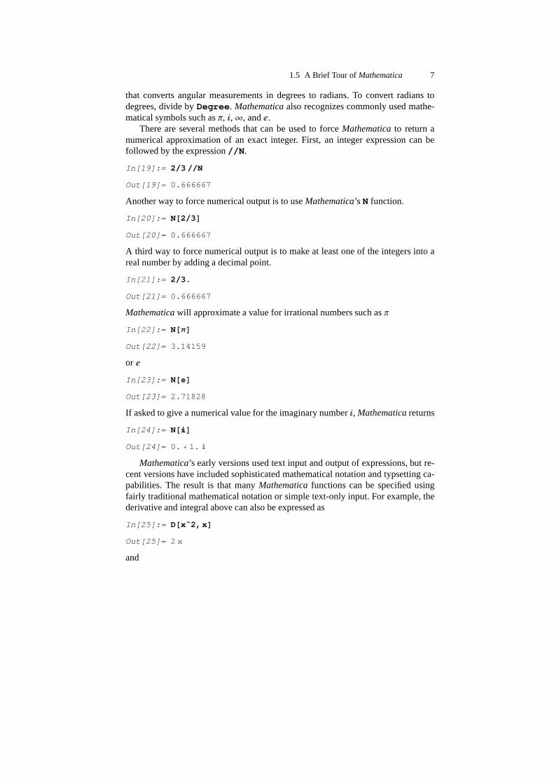
that converts angular measurements in degrees to radians. To convert radians todegrees, divide by Degree. Mathematica also recognizes commonly used mathe-matical symbols such as Π, �, �, and �.

There are several methods that can be used to force Mathematica to return anumerical approximation of an exact integer. First, an integer expression can befollowed by the expression //N.

In[19]:= 2/3 //N

Out[19]= 0.666667

Another way to force numerical output is to use Mathematica’s N function.

In[20]:= N�2/3�

Out[20]= 0.666667

A third way to force numerical output is to make at least one of the integers into areal number by adding a decimal point.

In[21]:= 2/3.

Out[21]= 0.666667

Mathematica will approximate a value for irrational numbers such as Π

In[22]:= N�Π�

Out[22]= 3.14159

or �

In[23]:= N��

Out[23]= 2.71828

If asked to give a numerical value for the imaginary number �, Mathematica returns

In[24]:= N��

Out[24]= 0. � 1. �

Mathematica’s early versions used text input and output of expressions, but re-cent versions have included sophisticated mathematical notation and typsetting ca-pabilities. The result is that many Mathematica functions can be specified usingfairly traditional mathematical notation or simple text-only input. For example, thederivative and integral above can also be expressed as

In[25]:= D�xˆ2,x�

Out[25]= 2 x

and


In[26]:= Integrate�2 x,x�

Out[26]= x2

The definite integral of 2 x from a � 3.0 to b � 7.2 can be specified as

In[27]:= Integrate�2 x,�x,3.0,7.2�

Out[27]= 42.84

Likewise, the square root of 2.8 can be represented by either

In[28]:=�2.8

Out[28]= 1.67332

or

In[29]:= Sqrt�2.8�

Out[29]= 1.67332

or

In[30]:= 2.81/2

Out[30]= 1.67332

Special symbols such as Π, �, and � can be represented using the text equivalents Pi,I, and E.

1.5.2 Vector and Matrix Operations

Mathematica treats vectors of symbols, integers, and real numbers as lists and ma-trices as lists of lists. A list of data might be

In[31]:= data � �1.2, 4.8, 2.8, 7.2, 9.1, 6.5

Out[31]= �1.2,4.8,2.8,7.2,9.1,6.5�

whereas one list is used to represent each row of a matrix using a Table.

In[32]:= m � ��a,b,�c,d

Out[32]= ��a,b�,�c,d��

Elements of lists or tables can be isolated using either Part or double square brack-ets ��. The first element in the second row of m is

In[33]:= Part�m,2,1�

Out[33]= c

or, equivalently,

In[34]:= m��2,1��

Out[34]= c


Matrices can also be filled with values following some functional relationshipby using the Table function.

In[35]:= Table�i � j, �i,1,3,�j,1,3�

Out[35]= ��1,2,3�,�2,4,6�,�3,6,9��

In[36]:= MatrixForm�%�

Out[36]=��

1 2 32 4 63 6 9

��

Matrices can be displayed in more traditional form using //MatrixForm orMatrixForm��.

In[37]:= m// MatrixForm

Out[37]= �a bc d�

In[38]:= MatrixForm�m�

Out[38]= �a bc d�

They can also be constructed by clicking on the matrix button in the Basic Inputpalette. Many of Mathematica’s functions are listable, meaning that they can beapplied to lists (or lists of lists). To calculate the square root of each element indata, for example, apply the square root function to the entire list.

In[39]:=�data

Out[39]= �1.09545,2.19089,1.67332,2.68328,3.01662,2.54951�

Squaring the list returns the original values.

In[40]:= %2

Out[40]= �1.2,4.8,2.8,7.2,9.1,6.5�

Chapter 3 discusses mathematical operations on matrices, including dot and crossproducts.


1.5.3 2-D and 3-D Graphing

Mathematica contains functions for 2-D and 3-D graphing of functions, lists, andarrays of data. The following statement plots sin x over the range of 0 � x � 2 Π.

In[41]:= Plot�Sin�x�,�x,0,2 Π�

1 2 3 4 5 6

-1

-0.5

0.5

1

Out[41]= -Graphics-

This statement adds a title and labels to the two axes.

In[42]:= Plot�Sin�x�,�x,0,2 Π,PlotLabel� > "Example Plot",

AxesLabel � �"x","sin x"�

1 2 3 4 5 6x

-1

-0.5

0.5

1

sin x Example Plot

Out[42]= -Graphics-


A different function, ListPlot, is used for lists of data. If a list of single val-ues is given, for example the list data defined above, ListPlot will assumethat they are dependent variables and that the independent variable has the values1, 2, 3 . . .

In[43]:= ListPlot�data,PlotStyle� > PointSize�0.02��

2 3 4 5 6

4

6

8

Out[43]= -Graphics-

The dots can be connected using the option PlotJoined � True.

In[44]:= ListPlot�data,PlotJoined � True�

2 3 4 5 6

4

6

8

Out[44]= -Graphics-

Here is a data list with x and y values.

In[45]:= ��1., 0.8,�2.9, 0.7,�3.2,0.7,�4.2, 0.5

Out[45]= ��1.,0.8�,�2.9,0.7�,�3.2,0.7�,�4.2,0.5��


In this case, Mathematica plots the first element of each pair as the independentvariable and the second element as the dependent variable.

In[46]:= ListPlot�%,PlotJoined � True�

1.5 2 2.5 3 3.5 4

0.55

0.6

0.65

0.7

0.75

0.8

Out[46]= -Graphics-

Functions of two variables can be visualized as 3-D surface plots, contour plots, ordensity plots.

In[47]:= Plot3D�Sin�x� Sin�y�,�x,0,2 Π,�y,0,2 Π,

ColorOutput � GrayLevel�

0

2

4

6 0

2

4

6

-1

-0.5

0

0.5

1

0

2

4

6

Out[47]= -SurfaceGraphics-

As with other Mathematica functions, options can be used to control the details ofthe plots. The plot below sets the number of points at which the function is evaluateto 50 instead of the default value of 25.



ColorOutput � GrayLevel,PlotPoints � 50�

0

2

4

6 0

2

4

6

-1

-0.5

0

0.5

1

0

2

4

6


and this one removes the mesh.


ColorOutput � GrayLevel,Mesh � False�

0

2

4

6 0

2

4

6

-1

-0.5

0

0.5

1

0

2

4

6


The Plot3D default is to shade surfaces using three simulated colored light sources(rendered here using gray levels; see Appendix C for a detailed discussion of color


and lighting). Setting Lighting � False removes the lighting and shades thesurface according to its height.


ColorOutput � GrayLevel,Lighting � False�

0

2

4

6 0

2

4

6

-1

-0.5

0

0.5

1

0

2

4

6


Setting Shading � False produces a wire-mesh plot and using Hidden�Surface � False renders the surface transparent.


ColorOutput � GrayLevel,Shading � False,

HiddenSurface � False�

0

2

4

6 0

2

4

6

-1

-0.5

0

0.5

1

0

2

4

6



To see a complete list of the options available for any Mathematica function, useOptions�function_name�.

In[52]:= Options�Plot3D�

Out[52]= �AmbientLight � GrayLevel 0�,AspectRatio � Automatic,

Axes � True,AxesEdge � Automatic,AxesLabel � None,

AxesStyle � Automatic,Background � Automatic,

Boxed � True,BoxRatios � �1,1,0.4�,

BoxStyle � Automatic,ClipFill � Automatic,

ColorFunction � Automatic,ColorFunctionScaling � True,

ColorOutput � Automatic,Compiled � True,

DefaultColor � Automatic,DefaultFont � $DefaultFont,

DisplayFunction � $DisplayFunction,Epilog � ��,

FaceGrids � None,FormatType � $FormatType,

HiddenSurface � True,ImageSize � Automatic,

Lighting � True,LightSources � ��1.,0.,1.�,

RGBColor 1,0,0��,��1.,1.,1.�,

RGBColor 0,1,0��,��0.,1.,1.�,

RGBColor 0,0,1��,Mesh � True,

MeshStyle � Automatic,Plot3Matrix � Automatic,

PlotLabel � None,PlotPoints � 25,

PlotRange � Automatic,PlotRegion � Automatic,

Prolog � ��,Shading � True,

SphericalRegion � False,TextStyle � $TextStyle,

Ticks � Automatic,ViewCenter � Automatic,

ViewPoint � �1.3,�2.4,2.�,

ViewVertical � �0.,0.,1.��


The functionContourPlot works in a similar manner, but with different options.

In[53]:= ContourPlot�Sin�x� Sin�y�,�x,0,2 Π,�y,0,2 Π,


0 1 2 3 4 5 60

1

2

3

4

5

6

Out[53]= -ContourGraphics-

Here is the same function plotted with 3, instead of the default 10, contours.


ColorOutput � GrayLevel,Contours � 3�

0 1 2 3 4 5 60

1

2

3

4

5

6



This time, without shading the contour intervals.


ColorOutput � GrayLevel,ContourShading � False�

0 1 2 3 4 5 60

1

2

3

4

5

6


Density plots display a function of two variables using continuous shades or colorsinstead of contour intervals. Here is one with the default mesh

In[56]:= DensityPlot�Sin�x� Sin�y�,�x,0,2 Π,�y,0,2 Π,


0 1 2 3 4 5 60

1

2

3

4

5

6

Out[56]= -DensityGraphics-


and one without the default mesh.

In[57]:= DensityPlot�Sin�x� Sin�y�,�x,0,2 Π,�y,0,2 Π,

ColorOutput � GrayLevel,Mesh � False�

0 1 2 3 4 5 60

1

2

3

4

5

6

Out[57]= -DensityGraphics-

The functions ListPlot3D, ListContourPlot, and ListDensityPlotproduce similar plots from 2-D matrices or arrays of data. None of these three ac-cept independent values, and the horizontal coordinates are simply row and columnnumbers. To illustrate, first fill a table with values of sin x sin y over the ranges0 � x � 2 Π and 0 � y � 2 Π, with grid increments of Π/10. The semi-colon is usedto suppress the output of the resulting table.

In[58]:= Table�Sin�x� Sin�y�,�x,0,2 Π, Π/10,�y,0,2 Π, Π/10�


Then, plot the results using ListPlot3D.

In[59]:= ListPlot3D�%,ColorOutput � GrayLevel�

5

10

15

20

5

10

15

20

-1

-0.5

0

0.5

1

5

10

15

20


To change the horizontal coordinates from row and column numbers, use theMeshRange option.

In[60]:= ListPlot3D�%%,ColorOutput � GrayLevel,

MeshRange � ��0,2 Π,�0,2 Π�

0

2

4

6 0

2

4

6

-1

-0.5

0

0.5

1

0

2

4

6



1.5.4 User-Defined Functions

Mathematica allows the definition of functions that can range from one-line state-ments to complicated programs involving logical operations, calculations, andgraphics. A simple example of a function to calculate the square of a numer is:

In[61]:= x2�x_� �� x2

The combined colon and equal sign, ��, delays the assignment of the value x2to x2until the function is executed, and is therefore different than x2 �x2. Once a functionis defined, it can be used just like any of the built-in Mathematica functions.

In[62]:= x2�9.5�

Out[62]= 90.25

An equivalent way to accomplish the same thing is to use the Function function

In[63]:= Function�x2,x2�

Out[63]= Function x2,x2�

In[64]:= x2�5�

Out[64]= 25

or, using Mathematica shorthand,

In[65]:= �#12�&

Out[65]= #12&

In[66]:= %�5�

Out[66]= 25

The shorthand version can produce very compact programs and is often used byexpert Mathematica programmers, but can also be very difficult for others to readand understand.

Mathematica contains a variety of functions useful for flow control in longerprograms – for example If, Do, While, and For – that can be used for traditionalprocedural programming. It also contains functions such as Map and Apply thatcan be used for functional programming. Here are four different ways to calculatethe sines of a table of real numbers:

In[67]:= values � Table�x,�x,10. �, 40. �, 10. ��

Out[67]= �0.174533,0.349066,0.523599,0.698132�

In[68]:= Map�Sin,values�

Out[68]= �0.173648,0.34202,0.5,0.642788�

In[69]:= Sin�values�

Out[69]= �0.173648,0.34202,0.5,0.642788�


In[70]:= Table�Sin�values��i��,�i,Length�values��

Out[70]= �0.173648,0.34202,0.5,0.642788�

In[71]:= Do�values��i�� Sin�values��i��,

�i,Length�values�� values

Out[71]= �0.173648,0.34202,0.5,0.642788�

Complicated multi-line programs can be built up using the Module function,which allows for local variables and functions to be defined. Here is a simple appli-cation of Module that takes a list of data, determines its length, calculates its meanand standard deviation, and then returns all three results in a list.

In[72]:= Example�data_� ��

Module��len, mean, dev,

len � Length�data�

mean �1

len

len

�i�1

data��i��

dev �1

len � 1

�len

�i�1

�data��i�� mean�2

Return��len,mean,dev�

�

Using the previously defined list data, the results are:

In[73]:= Example�data�

Out[73]= �6,5.26667,1.30833�

Outside of the module, however, the variables len, mean, and dev have no values.

In[74]:= �len,mean,dev

Out[74]= �len,mean,dev�

1.5.5 Data Import and Export

Mathematica can import and export many common kinds of data and image files.The general Import function can in most cases recognize file types and make theappropriate conversions.Import assumes that any file name ending in .dat containsrows and columns of data. For example, the file example.dat contains four rows eachconsisting of four columns of data.

In[75]:= Import�"/Users/bill/Mathematica_Book/example.dat"�

Out[75]= ��1,2,3,4�,�5,6,7,8�,�9,10,11,12�,�13,14,15,16��


If List is specified as the file format, however, Mathematica will treat the data asa single list.

In[76]:= Import�"/Users/bill/Mathematica_Book/example.dat",

"List"�

Out[76]= �1,2,3,4,5,6,7,8,9,10,11,12,13,14,15,16�

The file path name can be pasted into an Import statement by selecting Get FilePath. . . from the Input menu. The same syntax works for graphics files.

In[77]:= Import�"/Users/bill/Mathematica_Book/pako.jpg"�

Out[77]= -Graphics-

Using the syntax above, Mathematica will use the file suffix to identify the file for-mat. See the Mathematica documentation for information on files without suffixes.Graphics files do not appear until they are specifically shown using the Show func-tion.

In[78]:= Show�%�

Out[78]= -Graphics-

The Export function works similarly to the Import function except that both anexpression (the data or image to be exported) and a file name must be specified.

1.5.6 Mathematica Packages

Mathematica functions and programs can be stored as text files known as packagesand loaded when needed. The standard distribution of Mathematica includes dozensof packages with special functions for algebra, calculus, graphics, linear algebra, nu-merical mathematics, and statistics. To see a complete list of the standard packagesaccompanying Mathematica, bring up the Help Browser window, choose Add-ons

1.6 References and Recommended Reading 23

& Links in the far left column, then Standard Packages in the middle column. Theright column will contain a list of directories, each of which contains several add-on packages that can be loaded whenever they are needed. Additional packages areavailable from Wolfram Research, from other commercial developers, and in thepublic domain (generally downloadable from the internet). This book includes apackage named CompGeosci, which contains a number of functions for specializedplots and calculations as well as color functions that are useful for color graphics.Users can also write their own packages, although the details of package writing arebeyond the scope of this book.

Mathematica packages can be loaded in two ways. The first is to use<< package_name, which loads the specified package. This is generally notthe recommended method because problems can arise if a package is loadedmore than once during a Mathematica session. The preferred method is to useNeeds�package_name�, which loads parts of the package as needed and will notload part of a package more than once.

Package names can be specified either using their complete file path or, if theyare located along one of Mathematica’s default file paths, using their directory (con-text in Mathematica terms) and package name. For example, to load the packageDescriptiveStatistics from the Statistics directory (context) located along one of thedefault file paths, enter

In[79]:= Needs�"Statistics‘DescriptiveStatistics‘"�

Note that the `character is not a single quotation mark! It is the character locatedbeneath the tilde (~) character in the upper left hand corner of most keyboards.Tosee a listing of the default file path for the installation of Mathematica on yourcomputer,type $Path and press Enter.To see a list of the packages that have beenloaded during a given Mathematica session, type $Packages and press Enter.

1.6 References and Recommended Reading

Glynn, J. and Gray, T., 2000, The Beginner’s Guide to Mathematica Version 4: CambridgeUniversity Press.

Wolfram, S., 1999, The Mathematica Book (4th ed.): Cambridge University Press.

1 introduction to mathematica - bilder.buecher.de file2 1 introduction to mathematica imental data...

Documents