Redesign of the National Resident Matching ProgramProgram

We turn next to think about 

• Theory as an input to design d h it’ t th l i t• and why it’s not the only input, 

• and what some other inputs might be…

To put it another way, we want to think about what makes design difficult, taking as a case study the redesign of the NRMP.

Roth, A. E. and Elliott Peranson, “The Redesign of the Matching Market for American Physicians: Some Engineering Aspects of Economic Design,” American Economic Review, 89, 4, September, 1999, 748‐780.

Some NRMP "match variations:” What makes the NRMP different from a simple college admissions model is that it has complications which sometimes cause two positions to be linked to one another, and sometimes cause the number of positions to change. p g

In the first category of differences are couples, who submit rank orders of pairs of programs and must be matched to two positions;orders of pairs of programs and must be matched to two positions; and applicants who match to 2nd year positions and have supplemental lists which must then be consulted to match them to 1st year positions. 

In the second category are requests by residency programs to have g y q y y p gan even or an odd number of matches, and reversions of unfilled positions from one program to another.  2

These complications matter for two related reasons:

1. They may change the properties of the match; and

2. The clearinghouse algorithm must be designed to accommodate them

Let’s take a look at how we might model couples, for example (keeping in mind that we’ll eventually have toexample (keeping in mind that we ll eventually have to take account of all the match variations, not just couples…)p )

3

Married couples looking for two residencies weren’t an issue in the medical job market until the 1970’sj

Harry S. Jonas, MD, Sylvia I. Etzel, ”Undergraduate Medical Education,” JAMA, Aug 26, 1988, vol. 260, 8 1063‐1071, 3008. 4

8035/16,468=.49

Chart 4, http://www.aamc.org/data/facts/charts1982to2010.pdf

5

An initial “couples algorithm” in the 1970’sp g• Couples (after being certified by their dean) could register for the match as a couple.– They had to specify one member of the couple as the “leading member.”

– They submitted a separate rank order list of positions for each member of the couple

• The leading member went through the match as if single.g

• The other member then had his/her rank order list edited to remove positions not in the ‘same community’ as the one the leading member hadcommunity  as the one the leading member had matched to.– Initially the NRMP determined communities; in a later version when couples were still defecting couples couldversion, when couples were still defecting, couples could specify this themselves.

6

A similar algorithm is used in Scotland dtoday

• “Linked applicants• To accommodate linked applicants, a joint preference list is formed for each such pair, using their individual preference lists and the programme compatibilitypreference lists and the programme compatibility information. If such a pair, a and b, have individual preferences p1, p2, . . . , p10 and q1, q2, . . . , q10 respectively (with a the higher scoring applicant), thenrespectively (with a the higher scoring applicant), then the joint preference list of the pair (a,b) is (p1,q1), (p1,q2), (p2,q1), (p2,q2), (p1,q3), (p3,q1), (p2,q3), (p3 q2) (p9 q10) (p10 q9) (p10 q10) (except that(p3,q2), . . ., (p9,q10), (p10,q9), (p10,q10) (except that incompatible pairs of programmes are omitted) “

• http://www.nes.scot.nhs.uk/sfas/About/default.asp

7

But this didn’t work well for couples• Why?• The iron law of marriage: You can’t be happier thanThe iron law of marriage: You can t be happier than your spouse.

• Couples consume pairs of jobs. So an algorithm that only asks for their preference orderings over individualjobs can’t hope to avoid instabilities (appropriately redefined to include couples’ preferences)redefined to include couples  preferences)

• But even if we ask couples for their preferences over pairs of jobs, we may still have a problem: Roth (1984) b d h h f bl h bobserved that the set of stable matchings may be 

empty when couples are present.

8

A More Complex Market: Matching with Couples This model is the same as the college admissions model, except the set g , pof workers is replaced by a set of applicants that includes individuals and couples.

Denote the set of applicants by A = A1C, where A1 is the set of e ote t e set o app ca ts by , e e s t e set o(single) applicants who seek no more than one position, and C is the set of couples {ai, aj} such that ai is in the set A2 (of husbands) and aj is in the set A3, and the sets of applicants A1, A2, and A3 together make up theset A3, and the sets of applicants A1, A2, and A3 together make up the entire population of individual applicants, A' = A1A2A3. 

Each couple c={ai aj} in C has preferences over ordered pairs of positionsEach couple c={ai,aj} in C has preferences over ordered pairs of positions, i.e. an ordered list of elements of FxF.  The first element of this list is some (ri,rj) in FxF which is the couples' first choice pair of jobs for ai and ajrespectively and so forthrespectively, and so forth. 

Applicants in the set A1 have preferences over residency programs, and residency programs (firms) have preferences over the individuals in A'residency programs (firms) have preferences over the individuals in A , just as in the simple model discussed earlier.  (That is, firms view the members of a couple as two distinct individuals…) 9

A matching is a set of pairs in FxA‘.

Each single applicant, each couple, and each residency program submits to the centralized clearinghouse a Rank Order List (ROL) that is their stated preference ordering of acceptable alternativesthat is their stated preference ordering of acceptable alternatives.

A  matching  is blocked by a single applicant (in the set A1), or by id if h h i di id la residency program, if matches that agent to some individual or 

residency program not on its ROL.  

A matching is blocked by an individual couple (ai,aj) if they are matched to a pair (ri,rj) not on their ROL.  

A residency program r and a single applicant a in A1 together block a matching  precisely as in the college admissions market, if th t t h d t th d ld b th f t bthey are not matched to one another and would both prefer to be. 

10

A couple c=(a1,a2) and residency programs r1 and r2 block  if the couple prefers (r1,r2) to (c), and either r1 and r2 each would prefercouple prefers (r1,r2) to (c), and either r1 and r2 each would prefer to be matched to the corresponding couple member, or if one of them would prefer, and the other already is matched to the corresponding co ple member That is c and (r r ) block ifcorresponding couple member.  That is, c and (r1,r2) block  if

1. (r1,r2) >c(c); and if either 2. {(a1 (r1), and  a1 >r1 ai for some ai (r1)  or a1 is acceptable to 

r1 and |(r1)| < q1 } and either a2(r2) or {a2 (r2),  a2 >r2 ajfor some a (r ) or a is acceptable to r and |(r )| < q }for some aj (r2)  or a2 is acceptable to r2 and |(r2)| < q2}

or 3. a1(r1) and {a2 (r2), and a2 >r2 aj for some aj (r2)    or a2 is 1 ( 1) { 2 ( 2), 2 r2 j j ( 2) 2

acceptable to r2 and |(r2)| < q2} 

11

A matching is stable if it is not blocked by any individual or by a an individual and a residency program, or by a couple together with one or two 

dresidency programs

Theorem 5 11 (Roth ’84): In the college admissionsTheorem 5.11 (Roth  84): In the college admissions model with couples, the set of stable matchings may be empty.p y

Proof: by (counter)example. (Which was sufficient, when I didn’t have design responsibility…)

12

Example‐‐market with one couple and no stable matchings (motivated by Klaus and Klijn, and Nakamura (JET corrigendum 2009 to K&K JET 2005): j , ( g )

Let c=(s1,s2) be a couple, and suppose there is another single student s3, and two hospitals h1 and h2.  Suppose that the acceptable matches for each agent, in order of preference, are given by

c: (h1,h2);  s3: h1, h2,h hh1: s1, s3; h2: s3, s2

Then no individually rational matching μ (i.e. no μ that matches agents only to acceptable mates) is stable We consider two cases depending on whether theacceptable mates) is stable. We consider two cases, depending on whether the couple is matched or unmatched.

Case 1: μ(c)=(h1 h2) Then s3 is unmatched and s/he and h2 can block μCase 1: μ(c) (h1,h2). Then s3 is unmatched, and s/he and h2 can block μ, because h2 prefers s3 to μ (h2)=s2.

Case 2: μ (c)=c (unmatched).  If μ (s3)=h1, then (c, h1,h2) blocks μ. If μ (s3)=h2 μ ( ) ( ) μ ( ) , ( , , ) μ μ ( )or μ (s3)=s3 (unmatched), then (s3,h1) blocks μ.

13

Why is the couples problem hard?Why is the couples problem hard?• Note first that the ordinary deferred acceptance algorithm won’t in general produce a stablealgorithm won t in general produce a stable matching (even when one exists, and even when couples state preferences over pairs of positions)p p p p )– In the worker proposing algorithm, if my wife and I apply to a pair of firms in Boston, and our offers are held and I am later displaced by another worker myheld, and I am later displaced by another worker, my wife will want to withdraw from the position in which she is being held (and the firm will regret having 

d h l h ld h )rejected other applications to hold hers)– In the firm proposing algorithm, it may be hard for a couple to determine which offers to holdcouple to determine which offers to hold.

14

Furthermore, the following example shows that even when the set of stable matchings is non‐empty, it may no longer have the nice properties we’ve come to expect.

Matching with couples  (Example of Aldershof and Carducci, ’96)4 h i l {h1 h4} h i h i i4 hospitals {h1,…h4} each with one position;  2 couples {s1,s2} and {s3,s4}

Preferences:Preferences:h1 h2 h3 h4 {s1,s2} {s3,s4}S4 s2 s2 s2 h3h2 h2h1S3 s3 s4 s3 h2h3 h2h3S3 s3 s4 s3 h2h3 h2h3

S1 s1 h2h4 h1h3h3h4 h4h1u h3 h4h3u h2u h4h3 uh2 u

15

There are exactly two stable matchings:  h1,…h4 are either t h d tmatched to:

h1 h2 h3 h4(s4 s2 s1 s3) h1, h2, h4, {s1,s2} prefer this

or to

(s4 s3 s2 u) h3, {s3,s4} prefer this

So, even when stable matchings exist, there need not be an optimal stable matching for either side and employmentoptimal stable matching for either side, and employment levels may vary.

16

So we can start to note theorems about simple markets whose conclusions pdo not carry over to markets with the NRMP match variations (even just with couples).

In a simple matching market:

1. the set of stable matchings is always nonempty

2. the set of stable matchings always contains a "program optimal" stable matching, and an "applicant optimal" stable matching. 

3. the same applicants are matched and the same positions are filled at every stable matching.  

Similarly, strategic results about simple markets won’t carry over unchanged to the more complex medical market. p

17

Strategic behavior in simple markets (without match variations):

1. In simple markets, when the applicant proposing algorithm is used, but not when the hospital proposing algorithm is used, no applicant can possibly improve his match by submitting an ROL that is different from his trueimprove his match by submitting an ROL that is different from his true preferences.

2. In simple markets when the program proposing algorithm is used, every2. In simple markets when the program proposing algorithm is used, every applicant who can do better than to submit his true preferences as his ROL can do so by submitting a truncation of his true preferences.  

3. In simple markets, when the program proposing algorithm is used, the only applicants who can do better than to submit their true preferences are those who would have received a different match from the applicant proposing algorithm.  

Furthermore, the best such applicants can do is to obtain the applicant optimal t hmatch.

18

Descriptive Statistics: NRMP

1987 1993 1994 1995 1996APPLICANTS Primary ROL’s 20071 20916 22353 22937 24749Applicants with Supplemental ROL’

1572 2515 2312 2098 2436ROL’s Couples Applicants who are Coupled 694 854 892 998 1008PROGRAMSPROGRAMS Active Programs 3225 3677 3715 3800 3830Active Programs with ROL Returned

3170 3622 3662 3745 3758

Potential Reversions of Unfilled Positions

Programs Specifying R i

69 247 276 285 282Reversion Positions to be Reverted if Unfilled

225 1329 1467 1291 1272

Programs Requesting Even 4 2 6 7 8og a s eques g veMatching

4 2 6 7 8

Total Quota Before Match 19973 22737 22801 22806 22578 19

Because conclusions about simple markets can have counterexamples in the complex medical market, there were points at which we had to rely on computational explorations to see how close an approximation the simple theory provides for the complex marketthe complex market.

We relied on computation in three places:

Computational experiments were used in the algorithm design.

Computational explorations of the data from previous years were used to study the effect of different algorithmsyears were used to study the effect of different algorithms.

Theoretical computation, on simple markets, was used to d t d th l ti b t k t l it dunderstand the relation between market complexity and 

market size.20

Before we talk about computational experiments, let’s think about what class of algorithms we might want to explore.

The deferred acceptance algorithm for simple matching models gave us a one pass algorithm; it starts with everyone unmatched, and never cycles.  Our sense was that we weren’t going to be able to do that in the complexOur sense was that we weren t going to be able to do that in the complex problem, but rather that we’d have to build a stable matching (if one existed), resolving blocking pairs as we identified them.

E.g. if (m',w') is a blocking pair for a matching , a new matching  can be obtained from  by satisfying the blocking pair if m' and w' are matched to one another at their mates at (if any) are unmatched at and all otherone another at , their mates at  (if any) are unmatched at , and all other agents are matched to the same mates at  as they were at .

But even for the simplest models (e g the marriage model) this can cycleBut even for the simplest models (e.g. the marriage model) this can cycle, and might not converge to a stable matching (an observation originally due to Donald Knuth: see the discussion of Example 2.4 in Roth and Sotomayor).Sotomayor).

In the marriage model there’s a way around this problem. 21

Theorem 2.33 (Roth and Vande Vate): Let  be an arbitrary matching for (M W P) Then therean arbitrary matching for (M, W, P).  Then there exists a finite sequence of matchings 1,...,k, such that = is stable and for each i =such that  = 1,… k is stable, and for each i = 1,...,k‐1, there is a blocking pair (mi, wi) for isuch that follows from by satisfying thesuch that i+1 follows from i by satisfying the pair (mi, wi).

22

Elements of the proof:  Let 1 be an arbitrary (w.l.o.g individually rational) matching with blocking pair (m1,w1).  Let 2 be the matching obtained by satisfying the blocking pair, and define the set A(1) = {m1,w1}.

Inductive assumption: Let A(q) be a subset of MW such that there are no blocking pairs for q+1 contained in A(q), and such that  q+1 does not match any agent in A(q) to any agent outside of A(q).q+1 y g (q) y g (q)

Then if q+1 isn’t stable, there is a blocking pair (m’,w’) such that at most one of m’ and w’ is contained in A(q).    (If neither of {m’w’} is in A(q) let A(q+1) = A(q){m’w’} and let be obtained{m ,w } is in A(q), let A(q+1) = A(q){m ,w } and let q+2 be obtained from q+1 by satisfying the blocking pair (m’,w’).

Otherwise, one of the pair is in A(q), say m’ (in the other case the symmetric argument will apply).   Let A(q+1) = A(q){w’}.  Now run the deferred acceptance algorithm, just in the set A(q+1), starting with 

23

w’ proposing and continuing until a matching is reached with no blocking pairs among the members of A(q+1).  The output is q+2.  

This suggests a new class of algorithms, of which the deferred acceptance l i h i i lalgorithm is a special case. 

Start with an arbitrary matching , and select a subset A of agents such th t th bl ki i f t i d i A d d t t hthat there are no blocking pairs for  contained in A, and  does not match any agent in A to any agent not in A.  

(F l A ld b i f t t h d d i l(For example, A could be a pair of agents matched under , or a single agent, or the set of all men.)  

A new player say woman w is selected to join A If no man in A is part of aA new player, say woman w, is selected to join A.  If no man in A is part of a blocking pair with woman w, we may simply add her to A without changing the matching.  Otherwise, select the man m whom woman wmost prefers among those in A with whom she forms a blocking pair and form a newamong those in A with whom she forms a blocking pair, and form a new matching by satisfying this blocking pair.  If there is a woman w' = (m), then she is left unmatched at this new matching, and so there may now be a blocking pair (w' m') contained in A If so choose the blocking pair mosta blocking pair (w ,m ) contained in A.  If so, choose the blocking pair most preferred by w' to form the next new matching.  

24

The process continues in this way within the set A{w}, like the deferred acceptance algorithm with women proposing, satisfying the blocking pairs which p g p p g, y g g parise at each step until the process terminates with a matching i having no blocking pairs within Ai = S{w}.  

The process can now be continued with the selected set A growing at eachThe process can now be continued, with the selected set Ai growing at each stage.  At each stage, the selected set has no blocking pairs in it for the associated matching I, and so the process converges to a stable matching when Ak = MW.Ak  MW.

In the deferred acceptance algorithm with men proposing, the initial matching is the one at which all agents are single, and the initial set A is A=W.

In the deferred acceptance algorithm with men proposing, the welfare of the women rises monotonically throughout the algorithm. In this more general class of algorithms there is no parallel, since agents from either side may be introduced into the set A.  But the set A itself grows, so the algorithm converges.

So, we’ll be looking for an algorithm that accumulates agents not involved in blocking pairs…g p

25

Computational experiments in the algorithm design.The process by which the applicant‐proposing algorithm was designed p y pp p p g g g

is roughly as follows. First, a conceptual design was formulated and circulated for comment, based on the family of algorithms explored (for the marriage model) in Roth and Vande Vate (1990). ("Random Paths to Stability in Two‐Sided Matching," Econometrica, 58, 1990, 1475‐1480.)

To code this into a working algorithm, a number of choices had to be made, concerning the sequence in which operations would be conductedconcerning the sequence in which operations would be conducted.  

Most of these decisions can be shown to have no effect on the outcome of simplematches, but could potentially effect the outcome when the p , p yNRMP match variations are present. 

Consequently, we performed computational experiments before making sequencing choices.  

(Throughout the algorithm design process, we also posted progress reports on h b h h il bl ll i d i Si d ithe web, where they were available to all interested parties.  Since designs often have to be adopted my multiple constituencies, the design processmight be important…) 26

• Do sequencing differences cause substantial or predictable changes in the match result (e.g. do applicants or programs selected first do ( g pp p gbetter or worse than their counterparts selected later)?

• Does the sequence of processing affect the likelihood that an algorithm will produce a stable matching?algorithm will produce a stable matching?  

Experiments to test the effect of sequencing  were conducted using data from three NRMP matches: 1993, 1994, and 1995.three NRMP matches: 1993, 1994, and 1995.

The results were that sequencing effects existed, but were unsystematic, and effected on the order of 1 in 10,000 matches. 

(In the majority of years and algorithm sequences examined, the match was unaffected by changes in sequencing of algorithm operations, and in the majority of the remaining cases only 2 applicants received different matches.)

However sequencing decisions did influence the speed of convergence to a t bl t histable matching.

27

Based on the sequencing experiments described above, the following decisions were made pertaining to the design of the applicant proposing p g g pp p p galgorithm for the NRMP:

1 All single applicants are admitted to the algorithm for processing1. All single applicants are admitted to the algorithm for processing before any couples are admitted.

2. Single applicants are admitted for processing in ascending sequence b l dby applicant code.

3. Couples are admitted for processing in ascending sequence by the lower of the two applicant codes of the couple.

When a program is selected from the program stack for processing, the applicants ranked by the program are processed in ascending order by program rank number (i.e. in order of the program’s preferences).

28

29

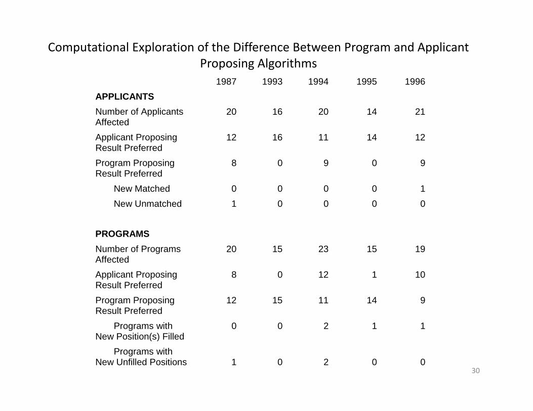
Computational Exploration of the Difference Between Program and Applicant Proposing Algorithms

1987 1993 1994 1995 1996APPLICANTS Number of Applicants Affected

20 16 20 14 21

Applicant Proposing Result Preferred

12 16 11 14 12

Program Proposing Result Preferred

8 0 9 0 9

New Matched 0 0 0 0 1 New Unmatched 1 0 0 0 0 PROGRAMSPROGRAMS Number of Programs Affected

20 15 23 15 19

Applicant Proposing Res lt Preferred

8 0 12 1 10Result Preferred Program Proposing Result Preferred

12 15 11 14 9

Programs with New Position(s) Filled

0 0 2 1 1New Position(s) Filled Programs with New Unfilled Positions 1 0

2 0 0

30

If this were a simple market, the small number of applicants p , ppwhose matching is changed when we switch from hospitals proposing to applicants proposing would imply that there was also little room for strategic behavior when it comes time toalso little room for strategic behavior when it comes time to state rank order lists.

f d f h l h l k hWe can find out if this is also true in the complex market with computational experiments.  It turns out that we don’t have to experiment on each individual separately, to put an upper p p y p ppbound on how many individuals could profitably manipulate their preferences.

(For the moment, we treat the submitted preferences as the true preferences—we’ll see in a minute why that is justified.)

31

Computational experiments to find upper bounds for the scope of strategic behaviorbehavior

Truncations at the match point (to check if examining truncations is sufficient in the multi‐pass algorithm…)

Difference in result for both the program proposing algorithm and the applicant proposing algorithm when applicant ROLs truncated at the match point:

1993 1994 1995

none 2 applicants improve, same positions filled

2 applicants improve, same positions filled

Difference in result for the program proposing algorithm when program ROLs truncated at the match point:

1993 1994 1995

none none 2 applicants do worse, same positions filled

32

Difference in result for the applicant proposing algorithm when program ROLs truncated at the match point:

1993 1994 1995

none3 applicants do worse, same number of positions filled, but not same positions [3 programs filled one less position 1 program filled 1 more

none

position, 1 program filled 1 more position, 1 program filled 2 more positions, 1 additional position was reverted from one program to another].

33

Results for Iterative Truncations of Applicant ROL’s just above the match point

1993 1994

Program Proposing Algorithm Applicant Proposing Program Proposing Algorithm Applicant Proposing

Truncated Truncated &  Truncated Truncated &  Truncated Truncated &  Truncated Truncated & Improved Improved Improved Improved

Run 1 17209 4546 17209 4536 17725 4935 17725 4934

Run 2 4546 2093 4536 2082 4935 2361 4934 2359

Run 3 2093 1036 2082 1023 2361 1185 2359 1183

Run 4 1036 514 1023 498 1185 602 1183 598

Run 5 514 258 498 241 602 292 598 287

Run 6 258 135 241 116 292 151 287 143

Run 7 135 73 116 52 151 75 143 66

Run 8 73 48 52 25 75 40 66 31

Run 9 48 34 25 12 40 27 31 17

Run 10 34 27 12 5 27 18 17 7

Run 11 27 24 5 2 18 14 7 3

Run 12 24 22 2 0 14 13 3 2

Run 13 22 22 13 13 2 234

The truncation experiments with applicants' ROLs yield the following upper bounds for the two algorithms in the years studied.

Upper limit of the number of applicants who could benefit by truncating their lists at one above their original match point:above their original match point: 

1987 1993 1994 1995 1996

Program‐Proposing Algorithmg p g g12 22 13 16 11

Applicant‐Proposing Algorithm0 0 2 2 9

As expected, more applicants can benefit from list truncation under the program‐proposing algorithm than under the applicant‐proposing algorithm.   Note that the number of applicants who could even potentially benefit from truncating their ROLs under the program‐proposing algorithm is in each year almost exactly equal to the number of applicants who received a preferred 

t h d th li t i t h (li 2 f T bl 2) Thi tmatch under the applicant proposing match (line 2 of Table 2).  This suggests that this upper bound is very close to the precise number that would be predicted in the absence of match variations. 35

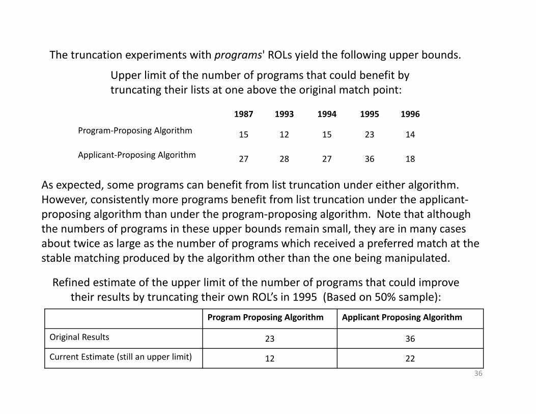
The truncation experiments with programs' ROLs yield the following upper bounds.

Upper limit of the number of programs that could benefit byUpper limit of the number of programs that could benefit by truncating their lists at one above the original match point:

1987 1993 1994 1995 1996

P P i Al ithProgram‐Proposing Algorithm 15 12 15 23 14

Applicant‐Proposing Algorithm 27 28 27 36 18

A d b fi f li i d i h l i hAs expected, some programs can benefit from list truncation under either algorithm. However, consistently more programs benefit from list truncation under the applicant‐proposing algorithm than under the program‐proposing algorithm.  Note that although the numbers of programs in these upper bounds remain small, they are in many cases p g pp , y yabout twice as large as the number of programs which received a preferred match at the stable matching produced by the algorithm other than the one being manipulated. 

Refined estimate of the upper limit of the number of programs that could improveRefined estimate of the upper limit of the number of programs that could improve their results by truncating their own ROL’s in 1995  (Based on 50% sample):

Program Proposing Algorithm Applicant Proposing Algorithm

Original Results 23 36Original Results 23 36

Current Estimate (still an upper limit) 12 2236

Residency programs have another dimension on which they can manipulate; they not only have to report their preferences, but also how many positions they wish to fill.  As we’ve seen in examples of the (simple) college‐admissions model and as in multi‐unitwe ve seen in examples of the (simple) college‐admissions model, and as in multi‐unit auctions, they may potentially benefit from demand reductions.

(And for an impossibility theorem on avoiding capacity manipulation, see Sonmez, Tayfun [1997], "Manipulation via Capacities in Two‐Sided Matching Markets," Journal of Economic Theory, 77, 1, November, 197 204 )197‐204.)

Revised Estimate of the Upper Bound of the Number of Programs That Could Improve Their Remaining Matches By Reducing Quotas 

1987 1993 1994 1995 1996

Program Proposing Algorithm 28 16 32 8 44

A li t P i Al ith 8 24 16 16 32Applicant Proposing Algorithm 8 24 16 16 32

This will be worth thinking about again—a small cloud on the horizon—when we id h i i f id hi f h iconsider what temptations may exist for residency programs to hire some of their 

people early, before the match.  If there are such temptations, they may not be counterbalanced by a tendency to do worse in the match, on the contrary, reducing demand may have small spillover benefits in the match for the remaining y p gcandidates…

37

Overall, the striking thing about all these computational results is how small the set of stable outcomes appear to be; i.e. how few applicants or programs are affected by a switch from program proposing to applicant proposing and how small are theswitch from program proposing to applicant proposing, and how small are the opportunities to misrepresent preferences or capacities.

But we don’t really understand the structure of the set of stable matchings when there are couples, supplementary lists, and reversion of positions from one program to another.  So there’s a chance that we’re making a big mistake here.  

For example, we know that program and applicant optimal stable matchings no longer b ’ b d h f bl h b l k h fexist, but we’ve been studying the set of stable matchings by looking at the outcomes of 

the program and applicant proposing algorithms.  Maybe the set of stable matchings isn’t all located between these two matchings when all the match variations are present; maybe the set of stable matchings just appears to be small because we don’t know where y g j ppto look.   

Even if our conclusions are correct, we’d like to know why.  Could it be some spooky interaction between the size of the market and the presence of complications?  Or does p pthe core simply get small as the market gets large, even in simple markets?

Two approaches:• Empirical: examine some simple marketsp p• Theoretical/computational: explore some artificial simple markets 

38

The Thoracic surgery match is a simple match, with no match variations.  It exactly fits the college admissions model; those theorems all apply.

Descriptive statistics and original Thoracic Surgery match results

1991 1992 1993 1994 1996

Applicant ROL’s 127 183 200 197 176Applicant ROLs 127 183 200 197 176

Active Programs 67 89 91 93 92

Program ROL’s 62 86 90 93 92

Total Quota 93 132 141 146 143

Positions Filled 79 123 136 140 132

Difference in Thoracic Surgery results when algorithm changed from program proposing to applicant proposing:

1991 1992 1993 1994 1996

none 2 applicants improve2 programs do worse

2 applicants improve2 programs do worse none none

39

Theoretical computation on a simple model

Simple model: n firms, n workers, (no couples) uncorrelated preferences, each worker applies to kuncorrelated preferences, each worker applies to k firms.

C(n) = number of workers matched differently at μF and μW

40

Large core with k=n: C(n)/n is the proportion of workers who receive different matches at different stable matchings, in a simple market (no couples) with n workers and n firms (each of which employs one worker) when preferences are uncorrelated and each preference list consists of all n agents on the other side ofuncorrelated and each preference list consists of all n agents on the other side of the market. (from Roth and Peranson, 1999)  Note that as the market grows large in this way, so does the set of stable matchings, in the sense that for large markets, almost every worker is effected by the choice of stable matching.

41

Small core of large markets, with k fixed as n grows: C(n)/n is the proportion of workers who receive different matches at different stable matchings in a simpleworkers who receive different matches at different stable matchings, in a simple market with n workers and n firms, when each worker applies to k firms, each firm ranks all workers who apply, and preferences are uncorrelated. (from Roth and Peranson, 1999).  Note that for any fixed k, the set of stable matchings grows small as n grows large.

42

The numerical results show us that C(n)/n gets small as n getsThe numerical results show us that C(n)/n gets small as n gets large when k is fixed, (even) for uncorrelated preferences.

And of course, in these simulated markets, we see that the core gets small not because of strategic behavior—these are the true g gpreferences.

This also implies that in large markets it is almost a dominant strategy for every agent to reveal his true preferences—only one in a thousand could profit by strategically mis‐stating preferences (if they had full information about all preferences).

43

In my class in the Spring of 2003, I posed the following as an Open Problem:  Prove:  The core gets small (in some expected value sense) 

h k l f h b f d ’ las the market gets large, if the number of interviews doesn’t also get large.

Two of the students in that class did so…Nicole Immorlica and Mohammad Mahdian, “Marriage, Honesty and Stability” Immorlica SODA 2005 53‐62Stability,  Immorlica, SODA 2005, 53‐62.

Theorem (Immorlica and Mahdian, 2003:) C id i d l i h d i hi h hConsider a marriage model with n men and n women, in which each woman has an arbitrary complete preference list, and each man has a random list of at most k women as his preference list (chosen uniformly and independently).Then, the expected number of women who have more than one stable husband is bounded by a constant that only depends on kstable husband is bounded by a constant that only depends on k (and not on n).(So, as n gets large, the proportion of such women goes to zero…) 44

More recently two former students have substantiallyMore recently, two former students have substantially generalized the result, to state that, as the market gets large, the opportunity for firms to manipulate either g , pp y ptheir preferences or their capacities gets small, in the sense that the proportion of firms with such an opportunity will go to zero.

Theorem (Kojima and Pathak AER 2009): In the limit asTheorem (Kojima and Pathak, AER 2009): In the limit, as n goes to infinity in a regular sequence of random (many‐to‐one) markets, the proportion of employers(many to one) markets, the proportion of employers who might profit from (any combination of) preference or capacitymanipulation goes to zero in the worker proposing deferred acceptance algorithm.

45

Still (mostly) open empirical puzzleStill (mostly) open empirical puzzle

• Why do these algorithms virtually always findWhy do these algorithms virtually always find stable matchings, even though couples are present (and so the set of stable matchingspresent (and so the set of stable matchingscould be empty)?

46

Stylized facts1 Applicants who participate as couples constitute a small1. Applicants who participate as couples constitute a small 

fraction of all participating applicants.2. The length of single applicants' rank order lists is small 

relative to the number of possible programsrelative to the number of possible programs.3. Applicants who participate as couples rank more programs 

than single applicants. However, the number of distinct programs ranked by a couple member is small relative to theprograms ranked by a couple member is small relative to the number of possible programs.

4. The most popular programs are ranked as a top choice by a small number of applicantssmall number of applicants.

5. A pair of hospital programs ranked by doctors who participate as a couple tend to be in the same region. 

6 E th h th li t th iti6. Even though there are more applicants than positions, many programs still have unfilled positions at the end of the centralized match.

7 A bl hi i i ll i i h k f7. A stable matching exists in all nine years in the market for clinical psychologists.

47

Two initial approachesTwo initial approaches

• Kojima Fuhito Parag A Pathak and Alvin EKojima, Fuhito, Parag A. Pathak, and Alvin E. Roth, " Matching with Couples: Stability and Incentives in Large MarketsIncentives in Large Markets

• Stability in large matching markets with complementarities (previously calledcomplementarities (previously called Matching with Couples ‐ Revisited) Itai Ashlagi Mark Braverman and AvinatanAshlagi, Mark Braverman and AvinatanHassidim(Extended abstract appears in EC 11.)

48

Random marketsRandom markets• A  random market is a tuple Γ=(H,S,C,  {Hⁿ}, k PQ ρ) where k is a positive integer (max lengthk,P,Q,ρ), where k is a positive integer (max length of ROL’s), P=(p{h}){h∈H} and Q=(q{h}){h∈H} are probability distributions on H, and ρ is a function hi h t f H twhich maps two preferences over H to a 

preference list for couples.• Hospitals’ preference orderings are essentiallyHospitals  preference orderings are essentially arbitrary, and take account of their capacities, and couples preferences are formed from their indi id al preferences (dra n from probabilitindividual preferences (drawn from probability distribution Q, different than P for singles), via an essentially arbitrary function ρ .

49

Random large markets• A sequence of random markets is (Γ¹,Γ²,…), where 

Γⁿ=(Hⁿ,Sⁿ,Cⁿ,≽{Hⁿ},kⁿ,Pⁿ,Qⁿ,ρⁿ) is a random market in which |Hⁿ|=n is the number of hospitals. | | p

Definition: A sequence of random markets (Γ¹, Γ², …) is regularif there exist λ>0, a ∈[0,(1/2)), b>0, r≥1, and positive integers k and κ such that for all n,integers k and κ such that for all n,  

1.kⁿ=k,  (constant max ROL length, doesn’t grow with n)2.|Sⁿ| ≤λn, |Cⁿ| ≤bna, (singles grow no more than 

proportionally to positions—e g λ>1 and couples growproportionally to positions—e.g. λ>1, and couples grow slower than root n)

3.κh≤κ for all hospitals h in Hⁿ (hospital capacity is bounded) 4 ( / )∈[(1/ ) ] d ( / )∈[(1/ ) ] f ll h it l h h′ i4. (ph/ph′)∈[(1/r),r] and (qh/qh′)∈[(1/r),r] for all hospitals h,h′ in 

Hⁿ. (The popularity of hospitals as measured by the prob of being acceptable to docs does not vary too much as the market grows i e no hospital is everyone’s favorite (inmarket grows, i.e. no hospital is everyone s favorite (in after‐interview preferences)

50

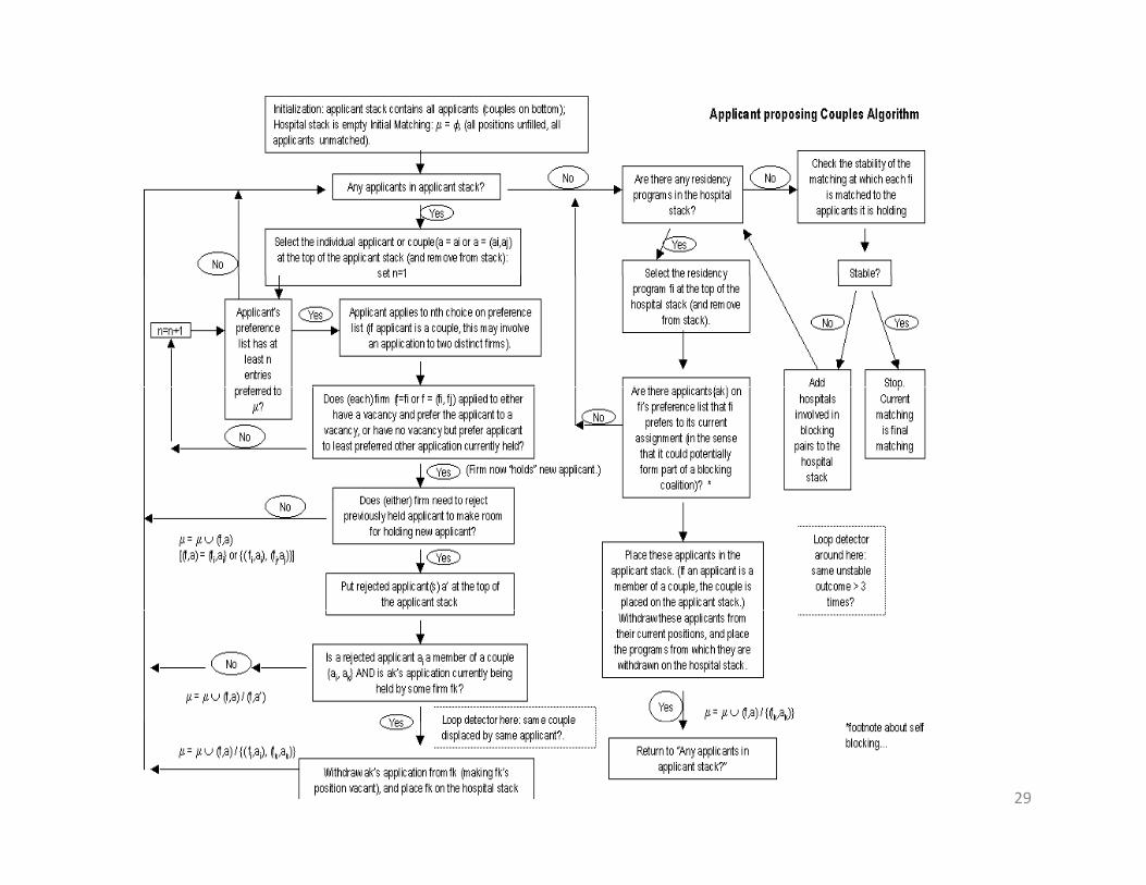
A (really simple) sequential couples algorithm (like left side of RP flow chart)algorithm (like left side of RP flow chart)

1.run a deferred acceptance algorithm for a sub‐market composed of all hospitals and single doctors, but without couples,

2.one by one, place couples by allowing each couple to apply to pairs of hospitals in order of their preferences (possibly displacing some doctors from their tentative matches), and

3 b l i l h di l d b l b ll i3.one by one, place singles who were displaced by couples by allowing each of them to apply to a hospital in order of her preferences.    

We say that the sequential couples algorithm succeeds if there is no instance in the algorithm in which an application is made to ainstance in the algorithm in which an application is made to a hospital where an application has previously been made by a member (or both members) of a couple except for the couple who is currently applying. Otherwise, we declare a failure and terminate th l iththe algorithm.

Lemma: If the sequential couples algorithm succeeds, then the resulting matching is stable.

51

Stable matchings exist, in the limitStable matchings exist, in the limit

• Theorem: Suppose that (Γ¹ Γ² ) is a regularTheorem: Suppose that (Γ ,Γ ,…) is a regular sequence of random markets. Then the probability that there exists a stable matchingprobability that there exists a stable matching in the market induced by Γⁿ converges to one as the number of hospitals n approachesas the number of hospitals n approaches infinity.

52

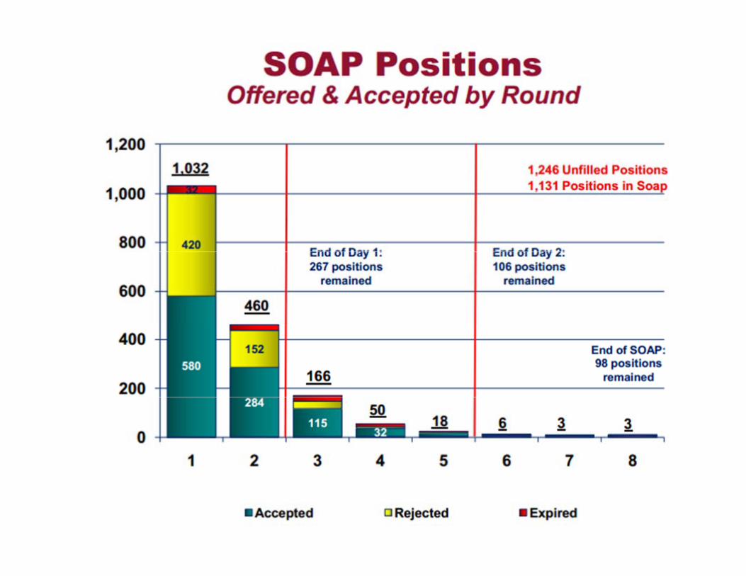
Key element of proofKey element of proof• if the market is large, then it is a high probability event that there are a large number of hospitalsevent that there are a large number of hospitals with vacant positions at the end of Step 2 (even though there could be more applicants than g pppositions) (i.e. the Scramble will remain important in large markets.)

• So chains of proposals beginning when a couple displaces a single doc are much more likely to terminate in an empty position than to lead to aterminate in an empty position than to lead to a proposal to a hospital holding the application of a couple member.p

53

Formal statementProposition: many hospitals have vacancies in large markets

There exists a constant  > 0 such that (1) the probability that, in a sub‐market without couples the doctor proposing deferred acceptancecouples, the doctor‐proposing deferred acceptance algorithm produces a matching in which at least n hospitals have at least one vacant position converges to one as n approaches infinity, and

(2) the probability that the sequential couples algorithm produces a stable matching and at leastalgorithm produces a stable matching and at least n hospitals have at least one vacant position in the resulting matching converges to one as n 

h fapproaches infinity.54

CorollaryCorollary

• Corollary: Suppose that (Γ¹ Γ² ) is a regularCorollary: Suppose that (Γ ,Γ ,…) is a regular sequence of random markets. Then the probability that the Roth‐Peranson algorithmprobability that the Roth Peranson algorithm produces a stable matching in the market induced by Γⁿ converges to one as the numberinduced by Γ converges to one as the number of hospitals n approaches infinity.

55

Stable Clearinghouses (those now using the  Roth Peranson Algorithm)

NRMP / SMS: Primary Care Sports Medicine (1994)Medical Residencies in the U.S. (NRMP) (1952)Abdominal Transplant Surgery (2005) Child & Adolescent Psychiatry (1995) Colon & Rectal Surgery (1984) Combined Musculoskeletal Matching Program (CMMP) 

Radiology • Interventional Radiology (2002) • Neuroradiology (2001) • Pediatric Radiology (2003) Surgical Critical Care (2004) 

• Hand Surgery (1990) Medical Specialties Matching Program (MSMP) • Cardiovascular Disease (1986) 

• Gastroenterology (1986‐1999; rejoined in 2006) 

Thoracic Surgery (1988) Vascular Surgery (1988) 

Postdoctoral Dental Residencies in the United States• Oral and Maxillofacial Surgery (1985))

• Hematology (2006) • Hematology/Oncology (2006) • Infectious Disease (1986‐1990; rejoined in 1994) • Oncology (2006) • Pulmonary and Critical Medicine (1986) • Rheumatology (2005) 

Oral and Maxillofacial Surgery (1985)• General Practice Residency (1986)• Advanced Education in General Dentistry (1986)• Pediatric Dentistry (1989)• Orthodontics (1996)Psychology Internships in the U.S. and CA (1999)gy ( )

Minimally Invasive and Gastrointestinal Surgery (2003) Obstetrics/Gynecology • Reproductive Endocrinology (1991) • Gynecologic Oncology (1993) • Maternal‐Fetal Medicine (1994) • Female Pelvic Medicine & Reconstructive Surgery (2001)

y gy p ( )Neuropsychology Residencies in the U.S. & CA (2001)Osteopathic Internships in the U.S. (before 1995)Pharmacy Practice Residencies in the U.S. (1994)Articling Positions with Law Firms in Alberta, CA(1993)Medical Residencies in CA (CaRMS) (before 1970)• Female Pelvic Medicine & Reconstructive Surgery (2001) 

Ophthalmic Plastic & Reconstructive Surgery (1991) Pediatric Cardiology (1999) Pediatric Critical Care Medicine (2000) Pediatric Emergency Medicine (1994) Pediatric Hematology/Oncology (2001)

Medical Residencies in CA (CaRMS) (before 1970)

********************British (medical) house officer positions• Edinburgh (1969)• Cardiff (197x)

56

Pediatric Hematology/Oncology (2001) Pediatric Rheumatology (2004) Pediatric Surgery (1992) 

• Cardiff (197x)

New York City High Schools (2003)Boston Public Schools (2006)

Self‐blocking couples:  A different kind of (modeling) problem that we spent a little time thinking about is raised by the following partial example:thinking about is raised by the following partial example:

Let C = {a1, a2} have preferences: (H1, H2), (H2, H3)

Suppose the relevant part of the hospital preferences areSuppose the relevant part of the hospital preferences areH1:  a1, …H2: a1, a2H3: a2, …

Consider a (partial) allocation that has C={a1,a2} matched to H2, H3.  That is, C gets it’s second choice, [(a1,H2), (a2,H3)]

Note that C would prefer the matching at which it was matched to H1,H2, i.e. [(a1,H1), (a2,H2)]

But {C, H1, H2} don’t block the original matching because H2 prefers a1 to a2.

But maybe we should think of a modified definition in which {C, H1, H2}does block the original matching, since C can withdraw a2 from H2…  As an administrative matter, C wouldn’t like to hear that they had gotten their second choice only because they had listed it as acceptable…

57

ScrambleScramble

• if the market is large then it is a highif the market is large, then it is a high probability event that there are a large number of hospitals with vacant positions atnumber of hospitals with vacant positions at the end of a centralized match with short preference lists (even though there could bepreference lists (even though there could be more applicants than positions) (i.e. the Scramble will remain important in largeScramble will remain important in large markets.)

58

59

60

61

62

63

64

65

66