wearable tactile pressure sensing for compression …
TRANSCRIPT

Wearable Tactile Pressure Sensing for Compression
Garments and Control of Active Compression
Devices
by
Steven Baron Lao
A thesis
presented to the University of Waterloo
in fulfillment of the
thesis requirement for the degree of
Master of Applied Science
in
Mechanical Engineering
Waterloo, Ontario, Canada, 2015
© Steven Baron Lao 2015

ii
Author’s Declaration
I hereby declare that I am the sole author of this thesis. This is a true copy of the thesis, including any
required final revisions, as accepted by my examiners.
I understand that my thesis may be made electronically available to the public.

iii
Abstract
Compression garments on the lower limbs have been used for the treatment of venous deficiencies for
centuries. More recently, healthy athletes have used similar garments for an edge in performance and
improved recovery times. The basis for their use is the increase of blood circulation that helps oxygenate
muscles. Active compression devices that apply intermittent compression are less prevalent but have the
potential to generate a greater impact on blood circulation. A new study into the effects of active
compression required the development of an active compression system that would apply intermittent
compression in a reliable manner.
In the present thesis, a control system to facilitate active compression and generate a positive impact on
blood circulation is pursued. This development involved setting up the timing of the compression and
implementing a controller that regulates the compression pressure. A new capacitive sensor for pressure
feedback to the controller is also evaluated.
In the resulting active compression system that was built, an electrocardiogram (ECG) and heel switch are
used to determine the timing of the compression. The ECG synchronizes the compression with the
heartbeat, while the heel switch prevents compression from being applied when the calf muscles are
contracted because the compression would not have an effect in that scenario. When the timing criteria is
met, sequential compression up the calf is applied with five inflatable cuffs to push the blood up the leg and
towards the heart. The pressure is sensed during each compression and used in an iterative learning
controller that regulates the amount of compression applied.

iv
Acknowledgements
I would like to acknowledge the many people who had contributed to my research and helped me on my
journey to complete this thesis.
Foremost, I would like to thank Professor Armaghan Salehian for the opportunity to work on this project
for my Master’s degree and providing the funding. Her relentless support and guidance has been vital to
my personal development and growth.
I am also appreciative to Dr. Keyma Prince and Professor Sean Peterson for their guidance and mentorship
on this project. The challenges they posed pushed me to be more critical and broaden my horizons.
To my lab mates, Mohammed Ibrahim, Blake Martin, Tim Pollock, and Hamza Edher, thanks for sharing
your thoughts, and bouncing ideas and encouragement during challenging moments. The friendly
atmosphere in the lab has made this experience much more enjoyable.
A special thanks to Professor Richard Hughson for providing access to his lab and equipment, which was
crucial to the collection of data. Also to Dr. Kathryn Zuj and Krysta Peralto for their help with the collection
of data in the lab.
Finally, I would like to thank everyone at StretchSense for their assistance in the development of the custom
pressure sensor.

v
Table of Contents
Author’s Declaration ..................................................................................................................................... ii
Abstract ........................................................................................................................................................ iii
Acknowledgements ...................................................................................................................................... iv
Table of Contents .......................................................................................................................................... v
List of Figures ............................................................................................................................................. vii
List of Tables ............................................................................................................................................... ix
Nomenclature ................................................................................................................................................ x
Chapter 1 Introduction ............................................................................................................................... 1
1.1. Motivation ..................................................................................................................................... 2
1.2. Scope of Work .............................................................................................................................. 2
1.3. Thesis Organization ...................................................................................................................... 3
Chapter 2 Background and Literature Review .......................................................................................... 4
2.1. Cardiovascular System .................................................................................................................. 4
2.2. Medical Compression Therapy ..................................................................................................... 7
2.2.1. Compression garments .......................................................................................................... 7
2.2.2. Intermittent pneumatic compression ..................................................................................... 8
2.3. Tactile Pressure Sensors................................................................................................................ 9
2.3.1. Pneumatic-based ................................................................................................................. 10
2.3.2. Piezoresistive ...................................................................................................................... 11
2.3.3. Strain Gauge ........................................................................................................................ 12
2.3.4. Piezoelectric ........................................................................................................................ 13
2.3.5. Capacitive ........................................................................................................................... 13
2.3.6. Summary ............................................................................................................................. 14

vi
Chapter 3 Active Compression System Control ...................................................................................... 16
3.1. Original Experimental Test Bed ................................................................................................. 16
3.2. Modifications to Experimental Test Bed .................................................................................... 19
3.2.1. Pressure Sensing System Testing ........................................................................................ 19
3.2.2. Timing of Actuation ............................................................................................................ 21
3.2.3. Compression Pressure Feedback ......................................................................................... 24
3.3. Results and Discussion ............................................................................................................... 25
Chapter 4 Pressure Sensing ..................................................................................................................... 29
4.1. Motivation for a new sensor........................................................................................................ 29
4.2. Capacitive Sensor ........................................................................................................................ 30
4.3. Experimental Methods ................................................................................................................ 30
4.4. Results and Discussion ............................................................................................................... 32
4.4.1. Stretch Sensor ..................................................................................................................... 32
4.4.2. Generation 1 ........................................................................................................................ 33
4.4.3. Generation 2 ........................................................................................................................ 34
4.4.4. Generation 3 ........................................................................................................................ 40
4.5. Temperature and Humidity Factors ............................................................................................ 45
4.6. Control Feedback with Gen 3 StretchSense Sensor .................................................................... 47
Chapter 5 Conclusions and Future Work ................................................................................................. 50
5.1. Conclusions ................................................................................................................................. 50
5.2. Future Work ................................................................................................................................ 51
References ................................................................................................................................................... 52

vii
List of Figures
Figure 1: Functional diagram of the cardiovascular system [10] .................................................................. 4
Figure 2: Diagram of heart [12] .................................................................................................................... 5
Figure 3: ECG waveform [14] ...................................................................................................................... 6
Figure 4: Skeletal muscle pump mechanism [15] ......................................................................................... 7
Figure 5: Normal and shear stresses on sensor ........................................................................................... 10
Figure 6: PicoPress bladder ........................................................................................................................ 11
Figure 7: Interlink FSR (top) and Tekscan FlexiForce (bottom) piezoresistive sensors ............................ 12
Figure 8: Strain gauge diagram ................................................................................................................... 13
Figure 9: Parallel plate capacitor model ..................................................................................................... 13
Figure 10: Pneumatic compression system diagram; adapted from [39] .................................................... 16
Figure 11: Five out of six pneumatic cuffs wrapped around the calf portion of the leg ............................. 17
Figure 12: One pressure sensing bank with four PicoPress bladders and one pressure transducer ............ 19
Figure 13: Test apparatus using two inflatable bladders ............................................................................. 19
Figure 14: Comparison of manometer reading and PicoPress sensor reading in test apparatus ................. 20
Figure 15: ECG R-peak detection ............................................................................................................... 22
Figure 16: Flow chart of smart timing algorithm ........................................................................................ 24
Figure 17: Active compression system overview ....................................................................................... 26
Figure 18: Iterative learning control applied to regulate the pressure by controlling the length of time the
solenoid is switched on. .............................................................................................................................. 27
Figure 19: ILC controller handling step changes in target pressure (step occurs at 10s mark) .................. 28
Figure 20: Diagram of test configurations for pressure sensor validation .................................................. 31
Figure 21: Piston test schematic ................................................................................................................. 31
Figure 22: StretchSense standard stretch-mode sensor and circuit board ................................................... 32
Figure 23: Gen 1 StretchSense pressure sensor with circuit board and battery .......................................... 34
Figure 24: A pair of Gen 2 StretchSense sensors with circuit board and battery ....................................... 35
Figure 25: Bladder test with Gen 2 sensors ................................................................................................ 36
Figure 26: Mass test repeated four times (Gen 2) ....................................................................................... 37
Figure 27: Piston test (Gen 2) ..................................................................................................................... 38
Figure 28: Bladder test (Gen 2)................................................................................................................... 39
Figure 29: Curvature test (Gen 2) ............................................................................................................... 40

viii
Figure 30: Testing protocol for applied load on sensor in the static tests ................................................... 41
Figure 31: Mass test (Gen 3) ....................................................................................................................... 42
Figure 32: Accuracy of Gen 3 sensor in mass test ...................................................................................... 43
Figure 33: Piston test (Gen 3) ..................................................................................................................... 43
Figure 34: Bladder test (Gen 3)................................................................................................................... 44
Figure 35: Curvature test (Gen 3) ............................................................................................................... 45
Figure 36: Gen 3 Mass test at 29°C and 26°C ............................................................................................ 46
Figure 37: No load capacitance vs temperature .......................................................................................... 47
Figure 38: ILC with StretchSense as feedback handling a 50 to 60mmHg step change ............................. 49

ix
List of Tables
Table 1: Qualitative summary of advantages and disadvantages of common pressure sensing modalities
[25-38] ........................................................................................................................................................ 14
Table 2: Sequence of cuff inflation to achieve “milking” effect................................................................. 18

x
Nomenclature
𝐴 – Area (m2)
BPM – Beats per minute
𝐶 – Capacitance (F)
DAQ – Data acquisition unit
DVT – Deep vein thrombosis
𝐸 – Young’s modulus (MPa)
ECG – Electrocardiogram
𝐻𝑅 – Heart rate
𝐼 – Current (A)
IPC – Intermittent pneumatic compression
𝐿 – Length (m)
myRIO – A National Instruments real-time controller
psi – Pounds per square inch (pressure)
𝑃 – Pressure (mmHg)
𝑅 – Resistance (Ω)
𝑡 – Time (s)
𝑇 – Temperature (°C)
𝑉 – Voltage (V)
𝜀0 – Vacuum permittivity (8.854 ∙ 10−12 F/m)
𝜀𝑟 – Relative permittivity
𝜖 – Strain (mm/mm)
𝜌 – Resistivity (Ωm)
𝜎 – Stress (Pa)

1
Chapter 1 Introduction
The circulatory system is a complex system that facilitates the distribution of nutrients to cells through
the body. The cardiovascular system is part of the circulatory system that is responsible for the transport
of blood. The circulation of blood is vital as it contains nutrients and oxygen to supply tissues and
carries waste away from them. The "Second Heart" is a mechanism that aids in pumping blood from
the lower legs back up to the heart and is important in maintaining adequate circulation in the lower
extremities.
The overarching objective of this research is to develop an active compression system to improve
venous blood flow in the lower extremities and study its effects on the human body. This compression
system is to be a non-invasive device that covers the calf and squeezes in a sequential manner from the
ankle to knee. The sequential compression up the leg is meant to mimic a “milking” action to stimulate
blood return through the veins, which in turn increases the overall blood flow. This increased blood
circulation may benefit muscle output and recovery as the muscles receive more oxygen and nutrients
to function. The increased blood flow and venous pressure may also benefit the heart as it does not need
to pump as hard to induce blood return from the lower extremities. Guyton and Jones noted that an
increase in the central venous pressure of several mmHg can increase cardiac output by threefold [1].
Compression therapy is commonly used to aid with venous deficiencies [2, 3]. Deficiencies in the
muscles or valves are fairly common and cause various problems that range from mild discolouration
to discomfort and development of ulcers or blood clots [2, 3]. This is due to blood pooling in the lower
leg and not circulating sufficiently in the veins. To date, the compression therapy has often involved
either passive compression or intermittent pneumatic compression. Passive compression uses stockings
or bandages that apply a fixed pressure while worn. Intermittent pneumatic compression on the other
hand has multiple compartments that fill with air periodically. These compression devices reduce the
local venous blood volume, which is redistributed closer towards the heart and allows the heart to refill
easier. The blood velocity in the veins also increase due to a decrease in vein diameter.
Compression for healthy users may also be beneficial, as suggested by the recent prevalence of
compression gear used by athletes. Producers of compression wear often makes claims of improved
performance, enhanced blood flow, better muscle oxygenation, reduced fatigue and faster recovery [4-
7].

2
In the following work, the development of a control system that applies active compression to the lower
extremities to assist the “Second Heart” and improve blood flow in the lower limbs is presented.
1.1. Motivation
The motivation for this work is to devise a system that can be used to study active compression in more
detail and determine if there is a benefit to their use. This system requires meticulous attention to
contributing factors and the control of variables. With the complexity of the human body there are many
variables to take into account.
In the engineering of the active compression system, providing consistent, repeatable pressures is
paramount. Another important factor is the timing of the compression. The pulse of the heart creates
pulsatile blood flow, so the timing of the compression relative to heartbeat must avoid impeding this
flow. This is difficult because the heart rate is a highly variable depending on what a person is doing.
Another important variable to control is the pressure being applied to the leg since the compression is
thought to be the driving factor that will improve blood flow. This necessitates a very consistent method
of applying compression to each participant in the future studies.
The shape, size and tissue compliance of the leg is different for each person. These factors are also
variable in time as a person flexes their muscles. This makes it difficult to apply pressure consistently
to a leg. A robust controller needs to be able to account for these variances and changes over time. To
regulate the pressure, the controller needs to accurately measure how much pressure is being applied to
the leg.
For the same reasons that is it difficult to apply pressure consistently, it is also difficult to measure the
pressure applied. Furthermore, the sensor needs to be low profile and soft so that it can rest between
the leg and compression system. So far, no ideal sensor has been found that can reliably and accurately
measure pressure applied to the leg in this type of application.
1.2. Scope of Work
The work presented in this thesis focuses on the control of the active compression system. The
biological implications and effects of the compression are being studied by others and are not within
the scope of the present thesis.
The scope of this thesis is specifically in the design of the control system to facilitate the active
compression protocol and the characterization of a new pressure sensor to measure the pressure applied.
The control system development includes controlling the timing and synchronization of the actuation
device and integrating a feedback loop from the pressure sensor to measure and regulate the amount of

3
pressure applied on the leg. The work involving the new pressure sensor is in the pursuit of a mobile
pressure sensing system that can sit between a person’s leg and the actuation device.
1.3. Thesis Organization
This thesis will be structured in the following manner:
Chapter 2 provides an overview of the state of the art in the areas of pressure sensing and
research in compression therapy. This information provided a baseline for the operating range
and key specifications of the control system and pressure sensors.
Chapter 3 presents the details of the control system that operates a pneumatic compression
system that is synchronized with the heart rate. Iterative Learning Control (ILC) is implemented
to regulate the pressure of the actuation on the calf.
Chapter 4 provides a detailed evaluation of a new pressure sensor to use as the feedback sensor
for the compression actuator.
Chapter 5 presents conclusions of the results and recommendations for future work in this
area.

4
Chapter 2 Background and Literature Review
This chapter presents background information on the operation of the cardiovascular system and the effects
of compression on the lower limbs. A review of technologies used for tactile pressure sensing is also
presented.
2.1. Cardiovascular System
The cardiovascular system is responsible for transporting blood cells, oxygen, nutrients, and waste products
throughout the body [8-10]. The main components of the cardiovascular system are the heart, blood, vessels
and lungs. Blood, which is the transport medium containing the essential substances for bodily function,
circulates through a closed network of vessels. One such function is to supply muscles with oxygen. A
functional diagram of the circulatory system is shown in Figure 1. The diagram shows the deoxygenated
blood (in blue) from the veins drawn into the right-side of the heart and ejected to the lungs. Lungs
oxygenate the blood cells (in red) before the blood re-enters the left-side of the heart. From the left-side of
the heart, the blood enters the arteries and the oxygenated blood cells are used by different parts of the body.
Figure 1: Functional diagram of the cardiovascular system [10]
5
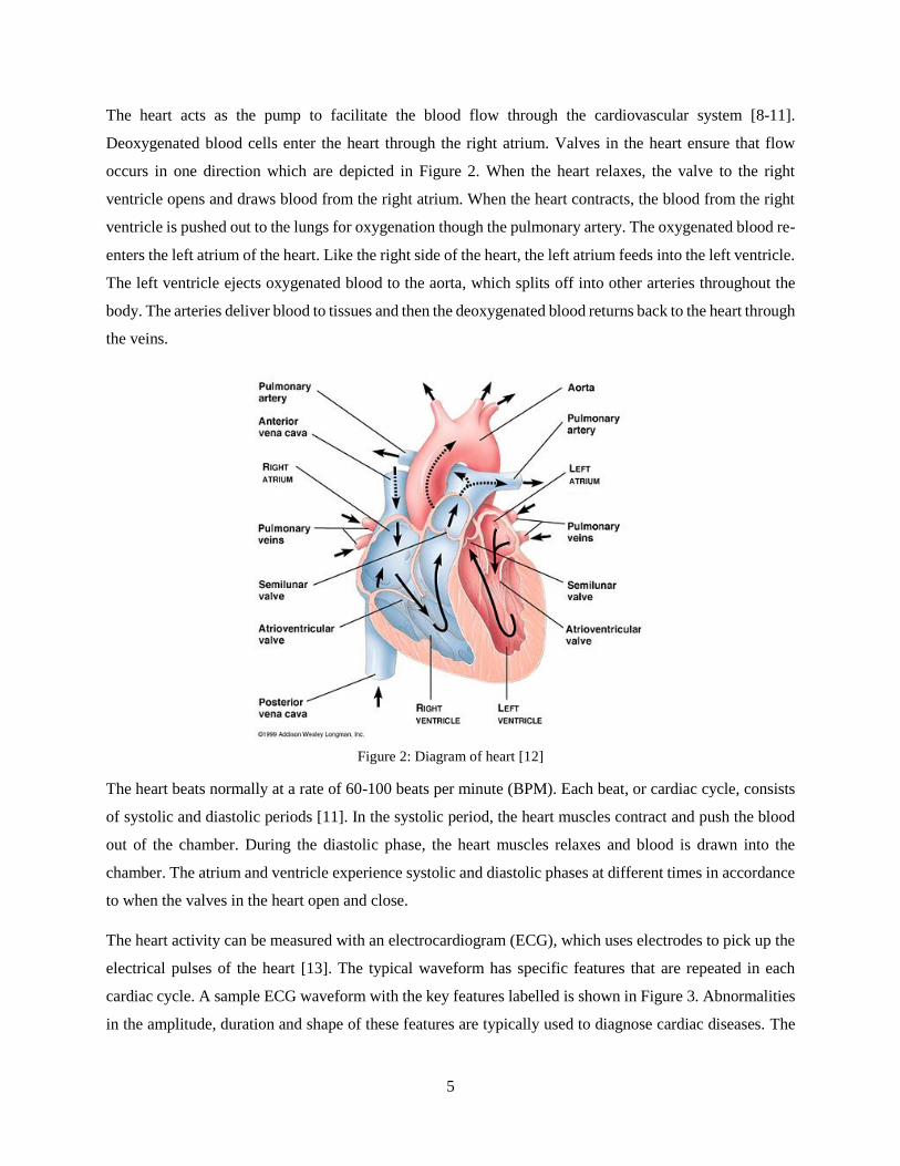
The heart acts as the pump to facilitate the blood flow through the cardiovascular system [8-11].
Deoxygenated blood cells enter the heart through the right atrium. Valves in the heart ensure that flow
occurs in one direction which are depicted in Figure 2. When the heart relaxes, the valve to the right
ventricle opens and draws blood from the right atrium. When the heart contracts, the blood from the right
ventricle is pushed out to the lungs for oxygenation though the pulmonary artery. The oxygenated blood re-
enters the left atrium of the heart. Like the right side of the heart, the left atrium feeds into the left ventricle.
The left ventricle ejects oxygenated blood to the aorta, which splits off into other arteries throughout the
body. The arteries deliver blood to tissues and then the deoxygenated blood returns back to the heart through
the veins.
Figure 2: Diagram of heart [12]
The heart beats normally at a rate of 60-100 beats per minute (BPM). Each beat, or cardiac cycle, consists
of systolic and diastolic periods [11]. In the systolic period, the heart muscles contract and push the blood
out of the chamber. During the diastolic phase, the heart muscles relaxes and blood is drawn into the
chamber. The atrium and ventricle experience systolic and diastolic phases at different times in accordance
to when the valves in the heart open and close.
The heart activity can be measured with an electrocardiogram (ECG), which uses electrodes to pick up the
electrical pulses of the heart [13]. The typical waveform has specific features that are repeated in each
cardiac cycle. A sample ECG waveform with the key features labelled is shown in Figure 3. Abnormalities
in the amplitude, duration and shape of these features are typically used to diagnose cardiac diseases. The

6
P wave marks the contraction of the atrium. The QRS complex represent the relaxation of the atrium and
contraction of the ventricles. Finally, the T wave represents the relaxation of the ventricles.
Figure 3: ECG waveform [14]
Although the cardiovascular system is a closed system, each part of the cardiovascular system is capable of
storing variable volumes of blood [8]. A change in blood pressure, flow, or volume in one section of the
body, such as the leg, does not immediately result in an overall increase. This behaviour is similar to the
effect of a capacitor in an electrical circuit. Like wires in a circuit, parts of the cardiovascular system are
joined by vessels and the flow through these vessels are governed by resistances and capacitances.
The largest reservoir of blood exists in the veins [9]. The venous system consists of low pressure vessels
due to the higher total resistance at the end of the circuit and their distance from the heart. To counteract
the low pressure and maintain return flow toward the heart, the veins contain one-way valves that prevent
retrograde flow [9, 11]. This is important as the venous blood in the legs must also counteract hydrostatic
pressure. When a person is standing, the blood in the lower limbs is pushed down due to gravity and the
elevation of the heart. The hydrostatic pressure (𝑃 = 𝜌𝑏𝑙𝑜𝑜𝑑𝑔ℎ, where 𝜌𝑏𝑙𝑜𝑜𝑑 is the density of blood, 𝑔 is
the gravitational acceleration, and ℎ is the elevation difference) is approximately 50-70mmHg.
The skeletal muscle pump (colloquially known as the “Second Heart”) is a mechanism that helps overcome
the effect of gravity [15]. When muscles around the veins contract, they expand and apply pressure on the
veins as seen in Figure 4 that forces blood through the series of valves and towards the heart. In individuals
with venous deficiencies, these valves are ineffective in preventing backflow. Compression therapy is
prescribed to alleviate these problems.

7
Figure 4: Skeletal muscle pump mechanism [15]
Furthermore, a strong link exists between the central venous pressure - the pressure of blood entering the
right atrium of the heart - and overall blood flow. Guyton and Jones pointed out that a change in central
venous pressure of a few mmHg may half or double cardiac output [1]. The venous system is believed to
have a powerful influence on the average blood flow around the body [9]. This effect is part of the reason
compression therapy is used to preload the blood to the heart and thereby increase blood flow [2].
2.2. Medical Compression Therapy
Compression therapy is often used to prevent the occurrence of deep vein thrombosis (DVT) and other
venous deficiencies [3, 16, 18]. DVT is the formation of blood clots in the deep veins of the legs due to
poor circulation or pooling of blood in the legs. The blood clot can cause pain or swelling, or cause
complications if the blood clot dislodges and creates a clot in the lungs (pulmonary embolism). Passive
compression is the application of a constant pressure through the use of compression garments, such as
socks or bandages. Meanwhile, active compression uses intermittent pressure which is through the use of
intermittent pneumatic compression (IPC).
2.2.1. Compression garments
In medical settings, an established practice for centuries to treat venous diseases is the use of compression
garments [2, 3, 16, 18]. The passive compression is applied using bandages or graduated compression
stockings. These garments apply a graduated pressure that is highest at the ankle and progressively
decreases toward the heart. This gradient pressure encourages the return of blood to the heart for

8
recirculation. Bandages must be applied by trained individual as the pressure and gradient is controlled by
the wrapping technique. On the other hand, graduated compression stockings can be worn like regular
socks. However, the individual variations in the shape and dimensions of each person’s leg can cause
improper pressure profiles [3]. A reverse gradient where the pressure is higher near the top of the sock can
produce a tourniquet effect and increase the risk of blood stasis [3].
The action of the compression garments is to counteract the hydrostatic pressure and reduce the diameter
of veins in the lower limbs [2, 18]. The external compression applied to the leg negates the pressure
differential due to the elevation of the heart. The reduction in the diameter of veins redistributes the volume
of blood from the superficial veins to deep veins, which improve muscle pumping and the flow in the deep
veins [19]. The reduced volume of blood in the legs leads to increased volume in the central parts of the
body and increased preload of the heart [2]. If the arterial flow is unaffected, the venous blood velocity also
increases with the decreased diameter of veins, which decreases the chances of stasis. It is important to note
that compression should not impede arterial flow. At conventional pressures, the arteries should be
unaffected as they are deeper under the skin and have higher blood pressures than the veins.
The pressure of compression garments ranges usually between 15-40mmHg at the ankle (highest pressure).
In certain situations, very strong pressures between 40-60mmHg can also be prescribed if needed. However,
the garments are more likely to be uncomfortable at higher pressures so lower compression pressures are
preferred. Investigations have found that the pressure to affect the vein diameter depends on the position of
the subject [2, 16, 18]. A person in the supine position would require less pressure to narrow the veins than
a person standing up. This is expected due to the hydrostatic pressure difference as discussed previously.
In the standing position, a pressure of approximately 30mmHg to start narrowing the diameter of the veins
and a pressure of approximately 75mmHg is enough to completely occlude the larger veins in the calf [16].
A recent study found that compression stockings had little effect on healthy subjects that did not suffer from
venous diseases [20]. The compression socks used in this study had a pressure range of 15-25 mmHg. The
main effect observed was a decrease in the blood volume in the legs, but no changes in overall blood flow.
The low pressure range of the stockings used in the study may have been a factor as noted previously it
would require 30mmHg to start seeing initial narrowing of the diameter of the veins for subjects that are
standing [18, 20].
2.2.2. Intermittent pneumatic compression
Intermittent pneumatic compression devices uses inflatable bladders that wrap around the leg and connect
to a pump that periodically inflates and deflates to apply pressure. IPC is an established and proven method
of preventing DVT [17, 21, 22]. Commercially available IPC products also differ widely in their coverage

9
(foot only, calf only, calf and thigh), number of cuffs, timing of actuation and pressure [21]. Most devices
inflate the cuffs to a pressure between 65-120 mmHg at a rate of three compressions per minute [23].
However, the air pressure in the cuffs has been shown to be inconsistent with pressure measurements taken
at the interface between the skin and the cuff and also shown to produce a non-uniform pressure on the leg
[21]. Nevertheless, the intermittent compression on the leg mimics the effect of the calf muscle pump as
described in Section 2.1, thereby preventing stasis and increasing venous return to the heart [17].
A pulse-synchronized IPC device was studied by Tochikubo and Kura [24]. Their IPC device consisted of
four cuffs that inflated individually at pressure between 40-80mmHg. One cuff would inflate during each
cardiac cycle starting from the bottom cuff to the top cuff. A photoplethysmogram clipped to the ear was
used to determine the blood flow and apply compression during ventricular diastole. The pulse-
synchronization was found to increase blood flow by 65% more than without compression. Without the
pulse-synchronization the blood flow only increased by 23%.
The results of this pulse-synchronized IPC device are encouraging for the method proposed in this research.
The compression in this work will be applied sequentially up the leg in one cardiac cycle instead of four
cycles, which should lead to higher blood flow. Other improvements to the timing will also be discussed in
the following chapter.
2.3. Tactile Pressure Sensors
Pressure sensors are often conceived as devices that measure the force per unit area that is holding a gas or
liquid in a vessel. Examples of such are tire pressure sensors and scuba tank pressure gauges. In these cases,
the nature of fluids permits a consistent and uniform excitation of the sensing element under the applied
pressure. However, the sensors that are desired for this application are tactile pressure sensors that measure
the force of physical contact between two objects. This physical contact can induce multiple components
of normal and shear forces in multiple axes as shown in Figure 5. Therefore, the physical interaction
between two objects is less predictable than the pressure in a fluid medium. Since the desired sensor should
be thin, the shear forces on the faces in the xy-plane are most susceptible to introducing errors. Moreover,
a sensor with a larger surface area would introduce errors if a non-uniform pressure is applied. The
flexibility and curvature of the sensor may also be an issue as it presents additional variables. The desired
pressure measurement of interest in this application is solely the normal component in the z-direction, but
these variables may obstruct the measurement.

10
Figure 5: Normal and shear stresses on sensor
In studies of compression garments, tactile pressure sensors are used to measure the compression pressure
applied by the garment. Tactile pressure sensors are also commonly used in the robotics industry and
commercial industry. These sensors are used for feedback on robotic manipulators and their end-effectors.
In commercial products, ergonomic studies are done to improve the comfort of consumer devices. These
tactile sensors operate with the use of pneumatic, piezoresistive, strain gauge, piezoelectric, or capacitive
technology [25, 26].
Each sensing technology has its own advantages and disadvantages. Furthermore, each sensing solution has
design trade-offs that are balanced and used to tailor sensors for a specific application. Due to these design
trade-offs and the variation in sensing requirements for different applications, direct comparisons of
specifications for each sensor technology is not possible [25, 26]. However, general characteristics for
performance and limitations of each technology is discussed below.
For compression garments, a consensus paper was generated to establish a list of desirable characteristics
for an ideal sensor to measure the interface pressure [27]. To date, no sensor has been able to meet all the
criteria. Some key characteristics are low cost, flexibility, durability, small surface area, thin profile, low
hysteresis, high sampling rate and little creep.
2.3.1. Pneumatic-based
Pneumatic-based sensors use bladders or compartments that are filled with a small volume of air [28]. These
are then connected to a pressure transducer through a rigid hose and kept sealed as a closed system when
placed at the measurement site. The pressure transducer is used to measure the pressure inside this closed
system. As the bladder is compressed, the volume of the bladder decreases and the pressure must increase
y x
z
σx
σy
σz
τxz
τxy
τyz
τzx τzy
τyx

11
(assuming temperature is constant). The assumption is made that the internal pressure measured by the
transducer is in equilibrium with the applied external pressure and therefore they are equivalent [28].
These sensors are commonly used in studies involving compression garments such as stockings and
bandages. Commercially available devices such as the Salzmann MST MKIV [29], MediGroup Kikuhime
[30], or Microlab PicoPress [31] (shown in Figure 6), are thin and flexible sensors that can be slipped under
compression devices to measure the interface pressure between the leg and compression device. Pneumatic-
based pressure sensors are currently the most popular method for measuring the pressure applied by
compression garments [32]. They have been found to have repeatable results within +/- 3mmHg [27, 31].
However, these sensors are sensitive to curvature which can lead to overestimated pressures by up to 150%
[32].
Figure 6: PicoPress bladder
2.3.2. Piezoresistive
Pressure sensitive inks, rubbers or elastomers that change in resistance under mechanical loads are used in
piezoresistive elements [26]. These piezoresistive sensors are connected to simple circuits that use the
relationship of the Ohm’s Law (𝑉 = 𝐼𝑅, where 𝑉 is the voltage (V), 𝐼 is the current (A), and 𝑅 is the
resistance (Ω)). In these circuits, the voltage or current is held constant, while the current or voltage is
measured to find the change in resistance.
Piezoresistive sensors are usually recognized for their thin profile, lightweight and low cost. Products such
as the Tekscan FlexiForce [33] and Interlink Electronics FSR [34] (both shown in Figure 7) have been
evaluated in studies for compression garments [32, 35]. These studies reported that the low-cost sensors
were acceptable for the requirements of their targeted applications. The piezoresistive sensors also had
negligible responses to thermal changes. However, the sensors suffered from hysteresis and drift, where a

12
constant load held for a period of time would cause a change in output. It was also found that the
piezoresistive sensors were drastically affected by curvatures under 32mm in radius. Furthermore, there is
a minimum load necessary to excite the sensor. This minimum activation load means that the sensor is
unreliable at measuring pressures under 15mmHg. Due to the errors attributed by repeatability, hysteresis
and linearity, the total error of the sensor is approximately +/- 10mmHg [32].
Figure 7: Interlink FSR (top) and Tekscan FlexiForce (bottom) piezoresistive sensors
2.3.3. Strain Gauge
Like piezoresistive sensors, strain gauges also respond in a change in resistance under mechanical strain
[26, 36]. Strain gauges are also thin and lightweight. Strain gauges consist of metallic traces that are applied
on a flexible substrate. The metallic trace is usually formed in a thin winding snake pattern as shown in
Figure 8. The resistance, 𝑅 (Ω), of the segments of the trace can be found by the equation:
𝑅 = 𝜌𝐿
𝐴 (1)
where 𝜌 is the resistivity (Ωm), 𝐿 is the length of the segment (m), and 𝐴 is the cross-sectional area (m2) of
the trace. As the segments are strained in expansion, the length would increase and the cross-sectional area
would decrease according to Hooke’s law. Both of these changes result in an increase in the resistance. The
inverse would be true for the case where the segments contract. Due to the trace pattern of the longer
segments along the sensitive direction of the strain gauge, changes in strain in that direction would have a
much larger response. Meanwhile, strains in the transverse direction would have a negligible response.
13
Figure 8: Strain gauge diagram
With the strain gauge bonded to another substrate with known elastic properties, the strain can be related
to the stress or pressure in the sensitive direction. Since the strain gauge is longest in the sensitive direction,
a pressure sensor that measures normal stress in the z-direction according to Figure 5 would result in a very
thick package. Additional challenges with strain gauges are the thermal and humidity sensitivity, and high
hysteresis due to their mechanical nature [26].
2.3.4. Piezoelectric
Piezoelectric materials exhibit a change in voltage under mechanical stress. Electric dipoles in the material
will align under mechanical deformation of the material, which creates a charge difference between the
electrodes of the material. Piezoelectric materials are known for their high sensitivity and fast response for
capturing high frequency content [26]. However, due to charge leakage, the voltage dissipates under static
loads; therefore piezoelectric sensors are mainly used for measuring dynamic loads [25, 26].
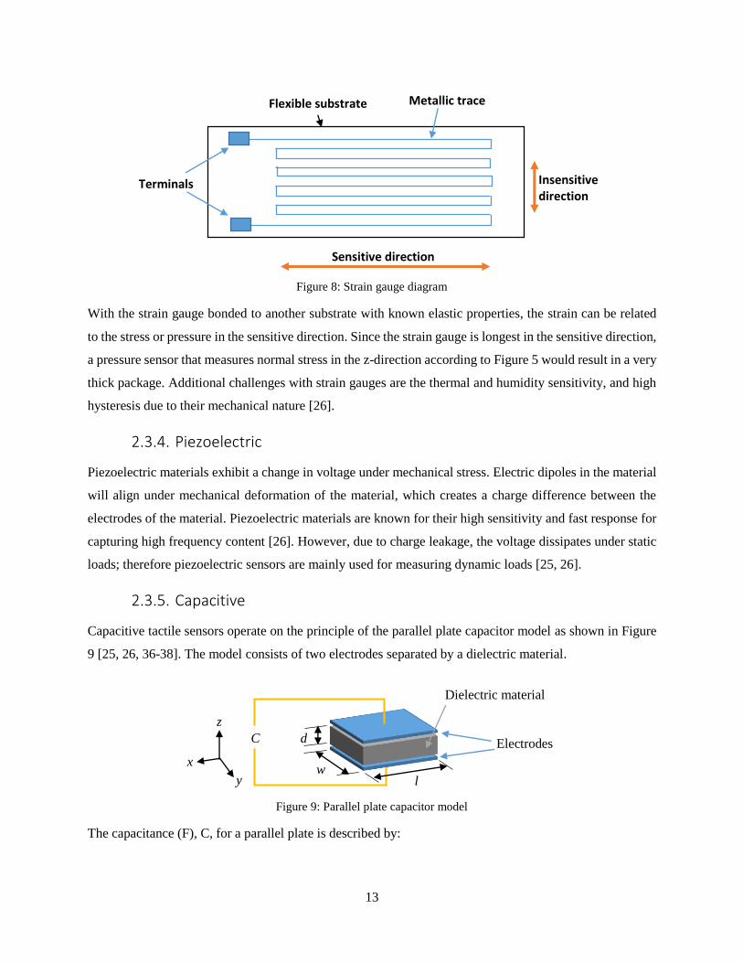
2.3.5. Capacitive
Capacitive tactile sensors operate on the principle of the parallel plate capacitor model as shown in Figure
9 [25, 26, 36-38]. The model consists of two electrodes separated by a dielectric material.
Figure 9: Parallel plate capacitor model
The capacitance (F), C, for a parallel plate is described by:
Flexible substrate Metallic trace
Terminals
Sensitive direction
Insensitive direction
Electrodes
Dielectric material
d
w l
C
x
z
y

14
𝐶 = 𝜀𝑟𝜀0𝐴
𝑑 (2)
where 𝜀𝑟 is the relative permittivity (unitless) of the dielectric, 𝜀0 is the vacuum permittivity (F/m), 𝐴 is the
area (m2) of the capacitor given by the length multiplied by the width, and 𝑑 is the thickness (m) of dielectric
material.
Compression of the capacitive sensor in the z-direction causes a decrease in the thickness and increase in
the area of the sensor according to Hooke’s Law [37]. Eqn 2 shows that both of these factors cause the
capacitance to increase. Capacitive sensors are highly sensitive to these changes. However, the accurate
measurement of capacitance can be a challenge and needs more complex circuitry. Measurements also
require filtering to reduce measurement noise [25, 26]. Hysteresis is a significant factor as the dielectric
material is often a silicone rubber that expands at a slower rate than it contracts [37]. An advantage of the
capacitive sensor is the temperature sensitivity is usually negligible [25, 38].
2.3.6. Summary
Tactile sensors need to be designed for a specific task because there are many sensor requirements that
significantly differ across applications. As mentioned previously, there can also be wide variances in the
capabilities and limitations of sensors even within the same category. Furthermore, the lack of a standard
method of characterizing sensors leads to difficulties in making direct comparisons between different
studies. This lack of consistency makes technological advancements hard to benchmark. Few studies have
been performed to evaluate metrological properties of these sensors [28]. Additionally, each application
reports results and specifications differently, which makes direct comparisons problematic. For that reason,
a qualitative summary of the advantages and disadvantages of the sensor technologies found in literature is
presented in Table 1.
Table 1: Qualitative summary of advantages and disadvantages of common pressure sensing modalities [25-38]
Advantages Disadvantages
Pneumatic-based Low cost
Thin profile
Latency
Large size
Sensitive to curvature
Piezoresistive Low cost
Thin profile
Flexible
Hysteresis
Drift
Low repeatability
Strain gauge Low cost
Good sensitivity
Flexible
Bulky size in direction of
measurement
Hysteresis
Temperature sensitive

15
Piezoelectric High sensitivity
High frequency response
Dynamic measurements only
Capacitive High sensitivity
Relatively low temperature
sensitivity
Susceptible to noise
Complex electronics
A significant challenge in the evaluation of these tactile pressure transducers is the lack of an established
method of applying pressure. Some studies may derive their results from well-controlled bench tests, or use
a sphygmomanometer wrapped around a solid cylinder. Both of these conditions are quite different from
in-situ tests against a person’s tissue, which has more variables. However, without a standard applicator of
pressure or measurement system to calibrate test results against, the challenge is to solve a circular
reference. This problem is like the chicken and egg dilemma. A method is proposed to evaluate a new
pressure sensor below whereby multiple bench test setups are used to introduce new variables individually
that mimic the expected in-situ condition. Each test setup can then be compared against each other as
verification of the results.

16
Chapter 3 Active Compression System Control
From the literature discussed in Chapter 2, the target pressure for the compression is between 20-100mmHg
as that is the common range that most compression devices apply. These compressions should make a
“milking” effect that pushes blood up the leg at every heartbeat. An active compression system that
consisted of a pneumatically powered compression system and pressure sensing system was built previously
for this application. Those systems and modifications to them that facilitate a more effective active
compression protocol are described in this chapter.
3.1. Original Experimental Test Bed
A pneumatic actuation system was previously built that could apply compression on the calf through the
use of six inflatable cuffs. A diagram of the pneumatic system is shown in Figure 10. A large air compressor
and air tank are used to supply the air to the system. A high flow pressure regulator (Control Air 700-BD)
reduces the upstream air pressure from the tank from 100psi to approximately 10-15psi. This regulated
pressure feeds into a manifold that branches out to the six inflatable cuffs. Each cuff is controlled by a 5-
way, 3-position pneumatic control valve (SMC VQZ3351). The control valves are plumbed to enable one
position that inflates the cuff, one position that keeps the cuff closed, and one position that vents the cuff
pressure to atmosphere. The control valves are solenoid actuated, which are activated by a data acquisition
unit (DAQ). The DAQ (NI cDAQ 9178) is programmed with LabVIEW.
Figure 10: Pneumatic compression system diagram; adapted from [39]

17
The inflatable pneumatic cuffs are designed similar to a sphygmomanometer (blood pressure cuff) except
it is constructed with a bicycle tire inner tube inside a fabric covering. The cuffs have a height of 2.5” to
allow the cuffs to be wrapped around the calf between the knee and ankle. Each cuff is a different length to
accommodate the differences in circumference along the calf. An image of the cuffs wrapped around a
subject’s leg is shown in Figure 11; typically only five cuffs are used as the sixth cuff sits very close to the
knee. The system facilitates a “milking” effect that pushes the venous blood upwards by sequentially
inflating the pneumatic cuffs from the ankle to the knee. The compression is applied very briefly to force
the venous blood through the valves of the veins and then the compression is released; one full compression
sequence takes 200ms from the time it starts to inflate the bottom cuff to when the top cuff deflates.
Figure 11: Five out of six pneumatic cuffs wrapped around the calf portion of the leg
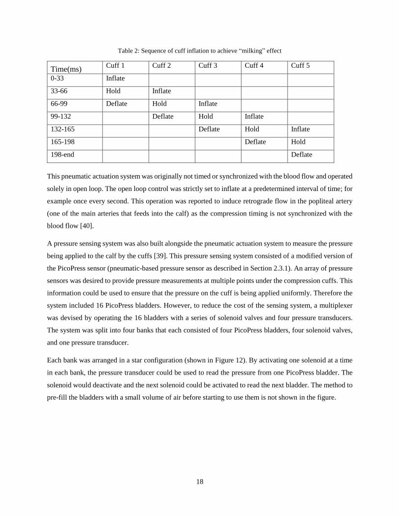
To achieve the “milking” effect, the inflation of each cuff is staggered as shown in the timeline on Table 2.
The three positions of the directional control valve allow the cuff to be in three states of inflation, hold, or
deflation. The hold state is where the cuff is kept sealed.
18
Table 2: Sequence of cuff inflation to achieve “milking” effect
Time(ms) Cuff 1 Cuff 2 Cuff 3 Cuff 4 Cuff 5
0-33 Inflate
33-66 Hold Inflate
66-99 Deflate Hold Inflate
99-132 Deflate Hold Inflate
132-165 Deflate Hold Inflate
165-198 Deflate Hold
198-end Deflate
This pneumatic actuation system was originally not timed or synchronized with the blood flow and operated
solely in open loop. The open loop control was strictly set to inflate at a predetermined interval of time; for
example once every second. This operation was reported to induce retrograde flow in the popliteal artery
(one of the main arteries that feeds into the calf) as the compression timing is not synchronized with the
blood flow [40].
A pressure sensing system was also built alongside the pneumatic actuation system to measure the pressure
being applied to the calf by the cuffs [39]. This pressure sensing system consisted of a modified version of
the PicoPress sensor (pneumatic-based pressure sensor as described in Section 2.3.1). An array of pressure
sensors was desired to provide pressure measurements at multiple points under the compression cuffs. This
information could be used to ensure that the pressure on the cuff is being applied uniformly. Therefore the
system included 16 PicoPress bladders. However, to reduce the cost of the sensing system, a multiplexer
was devised by operating the 16 bladders with a series of solenoid valves and four pressure transducers.
The system was split into four banks that each consisted of four PicoPress bladders, four solenoid valves,
and one pressure transducer.
Each bank was arranged in a star configuration (shown in Figure 12). By activating one solenoid at a time
in each bank, the pressure transducer could be used to read the pressure from one PicoPress bladder. The
solenoid would deactivate and the next solenoid could be activated to read the next bladder. The method to
pre-fill the bladders with a small volume of air before starting to use them is not shown in the figure.

19
Figure 12: One pressure sensing bank with four PicoPress bladders and one pressure transducer
During use, the PicoPress bladders can be placed under the compression cuffs to determine the amount of
pressure being applied to the leg. The combination of the compression system and pressure sensing system
to facilitate the active compression protocol and modifications to these two systems are discussed in
following section.
3.2. Modifications to Experimental Test Bed
To improve the performance and functionality of the test bed, three significant changes to the system were
made. First, the multiplexing functionality of the pressure sensing system was discarded after testing
demonstrated significant issues. Secondly, “smart timing” of the compression system was added to the
compression system to apply compression that was synchronized with the blood flow in the leg and calf
muscle activity. Finally, closed loop feedback is incorporated from the pressure sensing system to control
the cuff inflation.
3.2.1. Pressure Sensing System Testing
The pressure sensing system was initially tested with an apparatus whereby a PicoPress sensor was
sandwiched between two large inflatable bladders (diagram shown in Figure 13). The bladders are inflated
to a certain pressure by the hand pump and manometer, which is presumed to be equivalent to the external
pressure applied to the PicoPress sensor.
Figure 13: Test apparatus using two inflatable bladders
A comparison between the manometer and PicoPress sensor reading was in agreement with each other
within +/- 3mmHg when the PicoPress bladder was pre-filled with a sufficient volume of air as shown in
the results of Figure 14. However, if the PicoPress was pre-filled with too much air it would overestimate
Bladder Sensor
Manometer
and hand pump

20
the pressure applied. This occurred due to the thickness of bladder when it is overfilled. Under-filling the
PicoPress would cause an underestimation because the PicoPress bladder could be squeezed flat and there
would be no more air to build pressure in the closed system.
Figure 14: Comparison of manometer reading and PicoPress sensor reading in test apparatus
One issue with the configuration of the multiplexing system is the large volume of air between the PicoPress
bladder and the pressure transducer. Traditionally, a PicoPress bladder would be connected directly to a
pressure transducers through a small diameter tube. However, the multiplexing system incorporates a
manifold, which has a large volume relative to the PicoPress bladder, to branch off into the separate
bladders. This additional volume requires a larger volumetric change of the bladder to produce the same
change in pressure than the traditional PicoPress setup. The larger change in volume requires more pre-
filled air in the system to prevent the PicoPress bladders from becoming fully vacated under low pressures.
This also means that the sensor itself is thicker, which presents issues when the sensor is resting on curved
surfaces (as noted in Section 2.3.1). Furthermore, the higher change in volume requires more displacement
that produces a delayed sensor response. A delayed response is unfavourable for making dynamic
measurements and sensor feedback, which is discussed further later in this chapter.
Another issue with the multiplexing system was the fact that compressed air could travel between PicoPress
bladders and cause the measurements to be unreliable after cycling a few times. This can be clearly
demonstrated with the following example. Imagine the multiplexing system is pre-filled with a volume of

21
air and then closed off, and then one PicoPress bladder is kept under a constant load (such as 50mmHg)
and another bladder is kept under no load (0mmHg). If the multiplexing system switched between these
two bladders by activating and deactivating the corresponding solenoids, pressurized air would be trapped
in the manifold every time the loaded bladder is deactivated. When the unloaded bladder is activated, the
pressurized air from the manifold then enters the lower pressure bladder. As the multiplexer cycles through
the two sensors, the higher pressure air will enter the lower pressure bladder until the two reach equilibrium.
This would result in the two sensors reading the average pressure (25mmHg) even though the one sensor
was constantly under 50mmHg and the other was 0mmHg. This issue inherently makes the concept of
multiplexing unfeasible as the PicoPress sensor needs to be operated as a closed system. Therefore, the
multiplexing system was deactivated and only one PicoPress bladder is used in each bank of the pressure
sensing system.
3.2.2. Timing of Actuation
Initial testing of the compression system found that retrograde flow could be induced due to the poor timing
of compressions. To combat this effect, the compression should be applied at the end of ventricular systole
(refer to Section 2.1 and Figure 3), which is when the blood ceases to be ejected from the left side of the
heart and the right side draws blood from the veins. As noted previously, an ECG can be used to detect
electrical pulses of the heart and determine the state of the cardiac cycle.
Therefore, an ECG was selected to synchronize the compression system to the heart cycle. The desired
event is marked by the T-wave on the ECG. However, the most prominent features in an ECG waveform
are the QRS complex and R-peak. They are used to indicate the starting point for extracting other features
of the ECG waveform and diagnosis [41]. For example, the heart rate is calculated based on the time
(period) between successive R-peaks (called the R-R interval) using the following formula:
𝐻𝑅 =60
𝑡𝑅𝑅 (3)
where 𝐻𝑅 is the heart rate (BPM), and 𝑡𝑅𝑅 is the time between R-peaks (seconds).
By detecting each R-peak in real-time, a reference point within each cardiac cycle can be established. From
the reference point, a delay can be added to reach the systole to diastole transition. There are multiple
methods for detecting that have been established in literature [41]. For the fastest and simplest computation
method, a custom R-peak detection algorithm based on amplitude and time was selected. Since the R-peak
is represented by a very sharp spike, the algorithm looks at a 50ms window and searches for an occurrence
where three conditions are met. The first condition is for a maximum at the middle of the window. The
second condition is for the maximum to be greater than the set threshold. The final condition is for the start

22
and end of the window to have a value less than the threshold. These conditions would result in a triangular
profile in a short time period. A 300ms timeout after the detection of an R-peak was added to prevent any
possible false positive detections in that short amount of time (a 300ms period corresponds to a heart rate
of 200BPM).
To test this algorithm, it was run in MATLAB on a sample ECG signal sourced through a Collins ECG
machine, which outputs an amplified and filtered the signal from the ECG leads on the person’s body. A
snapshot of a five second ECG window is shown in Figure 15 where a threshold of 1V was used. In two
separate five minute ECG samples, the algorithm was able to detect 100% of the R-peaks.
Figure 15: ECG R-peak detection
For the live system, a National Instruments myRIO was used as the controller that would read signals from
the ECG machine and run the R-peak detection algorithm in real-time at a rate of 1000Hz. At the detection
of the R-peak, the myRIO would wait a period of time and then send a signal to the compression system to
start a compression sequence.
The delay between the detection of the R-peak and the start of one compression sequence is added to make
sure the blood is no longer flowing down the arteries of the leg when compression is applied. This delay
has two components. The first being the time between heart contractions (marked by the R-peaks) to when
the blood stops exiting the left ventricle. This time is believed to be a constant fraction of the heart rate or
the R-R interval. For a shorter R-R interval, the length of time that the blood exits the heart should also be
shorter. However, the R-R interval for each beat is unknown at the time of operation since knowledge of
the time of the next beat would require a non-causal system. Therefore, instead the time of the previous R-
R interval is used for the calculation. The second component of the delay is the pulse wave delay between
when the pulse occurs at the heart to when it reaches the leg. Therefore the delay algorithm is:
𝑡𝑑𝑒𝑙𝑎𝑦,𝑖 = tRR,i−1 ∗ k𝑓𝑎𝑐𝑡𝑜𝑟 + t𝑝𝑢𝑙𝑠𝑒 𝑤𝑎𝑣𝑒 𝑑𝑒𝑙𝑎𝑦 (4)
23
where 𝑡𝑑𝑒𝑙𝑎𝑦,𝑖 is the time that the controller waits after the detection of an R-peak to trigger the compression
sequence (in seconds), 𝑡𝑅𝑅,𝑖−1 is the R-R interval of the previous heartbeat (seconds), the k𝑓𝑎𝑐𝑡𝑜𝑟is the
constant fraction of the R-R interval. k𝑓𝑎𝑐𝑡𝑜𝑟 and t𝑝𝑢𝑙𝑠𝑒 𝑤𝑎𝑣𝑒 𝑑𝑒𝑙𝑎𝑦 are variables that can be modified on the
fly using the active compression system’s interface. The pulse wave delay is different for each person due
to the complexity of the cardiovascular system, so this delay is measured just prior to the use of the active
compression system. The measurement is taken with the aid of a Doppler ultrasound that senses the arterial
blood flow in the leg. By taking a few sample waveforms of the blood flow in the leg and plotting it with
the trigger signal for the compression system, the variable for the pulse wave delay can be increased or
decrease until the trigger signal overlaps with the point when the pulsatile blood flow in the leg is zero.
The synchronization with the heartbeat and the additional delay facilitate compression while blood is
returning to the heart. However, another element to consider for the smart timing of the active compression
system is the muscle activity in the calf. As described in Section 2.1, the skeletal muscle pump supplements
venous blood flow when muscles contract and squeeze blood through a series of valves in the veins. The
compression system would not have an effect when the calf muscles are already contracted since the blood
is squeezed through the veins. Thus, the compression system should not be run when the calf muscle is
contracted to reduce wasted energy.
The muscle activity is detected with a simple switch that is placed at the heel of the subject. When the
subject raises their heel, the calf muscles are activated and contracted. Whereas the calf muscles will be
relaxed when the heel is down on the floor. The switch used for this application is a piezoresistive sensor
(introduced in Section 2.3.2). These sensors detect the pressure being applied to them with low accuracy,
but the desired information from the sensor is a coarse measurement of whether the heel is up or down on
the floor. So the sensor is connected to a Schmidt trigger to convert the analog signal to a digital signal,
which is read by the myRIO. When the heel is down and the correct timing for the blood flow in the leg
occurs, the trigger to the compression system will be sent. If the heel is up, then the trigger signal will not
be sent.
The operations and decisions made by myRIO to achieve the desired smart timing described in this section
is depicted by the flow chart in Figure 16.

24
Figure 16: Flow chart of smart timing algorithm
3.2.3. Compression Pressure Feedback
The third major improvement to the active compression system is the addition of feedback control to
regulate the pressure applied by the pneumatic compression system. As outlined in Section 3.1, the pressure
of each cuff is controlled by a pressure regulator and a pneumatic directional control valve. There are a few
challenges to achieve the “milking” sequence (shown in Table 2) in a 200ms window due to the speed that
events must take place.
For the cuff to apply the desired pressure in the short period of time, the pressure regulator needs to be set
higher to maintain a high flow rate of the air travelling through the hoses. Therefore, in this application the
regulator cannot be used to set the compression pressure like in a pneumatic cylinder where a regulator
controls its force. Instead, the directional control valve opens and closes after a set period of time to stop
the cuff from inflating further.
However, due to the different lengths of the cuffs, the pressure in each cuff is not the same when inflated.
The larger cuffs would need more time to inflate as the volume is larger. Furthermore, the compliance of
the calf would have an effect on the inflation of the cuffs. Due to muscle and tissue composition, the
compliance of the leg varies significantly. For example, the front part of the leg is usually bony whereas
the back is more compliant. In addition, the muscle activity changes the shape and compliance of the leg.
The circumference of the leg changes as muscles contract and muscles reposition under the skin. These
variations make it challenging to maintain the pressure of the cuffs.
Furthermore, pneumatic systems are highly nonlinear systems due to the compressibility of air [42]. The
compressibility of air makes the system response sensitive to external loads and temperature changes [42].
The inflatable bladder in this case would be affected by different external loads through the changes in

25
compliance of the leg. Temperature will also be a factor as the person’s body temperature changes over
time, especially if the user is exercising.
To apply the correct pressure reliably and consistently, a feedback mechanism was developed to control the
inflation of the compression cuffs. This mechanism melded the compression and sensing systems since the
two would operate together.
Due to latencies in the control valve activation and slow response time of the pressure sensor, the control
loop of the actuator cannot operate based on the immediate feedback. A traditional methods, such as a PID
controller, would not work in this scenario. The control valve uses a solenoid coil to help switch the position
of a sliding spool that redirects air between the ports of the valve. The time to charge the solenoid coil and
move the spool takes up to 35ms to operate [43]. Even though it takes up to 35ms to fully complete the
switch, air will start to pass through during the transition. This makes it possible to inflate the cuffs for
33ms even though the switch is not fully completed. The delay from the sensor input also makes it difficult
to use immediate sensor feedback to control the inflation.
Instead, the feedback operates on an iterative learning control (ILC) strategy to regulate the maximum
pressure that the cuff applies in each compression cycle. The ILC method works by correcting the control
signal based on the control signal and error measured in the previous iteration. ILC controllers are regularly
used in repetitive operations since the error will theoretically converge to zero over many iterations [42].
The control law for the controller can be written as:
𝑢𝑖 = 𝑢𝑖−1 + 𝐾(𝑒𝑖−1) (5)
where 𝑢 is the control signal, 𝑖 is the iteration, 𝑒 is the error from the target pressure and 𝐾 is the correction
function. The length of time each solenoid is enabled and inflating the bladder is the control signal that is
corrected iteratively in this case.
In this application, the compression system’s DAQ will record the pressures read by the PicoPress sensors
from the start of compressions to 100ms after compressions end. The extra 100ms is to account for the
delay in the response time of the sensor. After collecting the pressure data, it determines the maximum
pressure each cuff exerted and calculates a new timing for each control valve.
3.3. Results and Discussion
The complete active compression system with the modifications described in the previous section is called
the “smart active compression system”. A diagram that outlines the system is shown in Figure 17. The
diagram shows the ECG and heel switch that are used to synchronize the compression with the blood flow
in the leg. The compression system also uses four of the PicoPress sensors to determine the time to actuate

26
the directional control valves that inflate the cuffs (potential improvements to the pressure sensing system
are pursued in the next chapter). As a temporary stopgap due to the missing sensor for cuff 3, the time of
that control valve is the average of the 2nd and 4th cuff.
Figure 17: Active compression system overview
An example of the ILC controller operating during a pilot test is shown in Figure 18. In this test the pressure
from one of the cuffs is measured with a PicoPress sensor as the compression system is synchronized with
the heart rate and muscle activity. The brief pauses after each three or four compressions is due to pauses
when the muscle calf is exerted and no compression is applied. As shown in the figure, the length of time
that the solenoid is on to inflate the cuff when the compression is applied is adjusted after each cycle if
necessary to maintain the desired target pressure.
ECG
Heel Switch
Compression Actuation
Pressure Sensing
Cuff 5
Cuff 4
Cuff 3
Cuff 2
Cuff 1
Sensor 5
Sensor 4
Sensor 2
Sensor 1
Pulse wave delay
Feedback
Knee
Ankle

27
Figure 18: Iterative learning control applied to regulate the pressure by controlling the length of time the solenoid is
switched on.
One advantage of the ILC controller is the ability to use actuation or sensor systems that have a slower
response time since the control feedback is dependent on the response in the previous cycle. Moreover, the
response time of the future wireless actuation and sensing systems may also be hindered by latency in
transmissions.
As a safety feature, the ILC controller also samples the pressure measurements in real time and will stop
inflating the cuffs if the measurement has already reached the target pressure. Therefore, the framework for
a bang-bang controller is also implemented in such case that actuation and sensor solutions that have a
faster response times are used in the future. Another safety addition is a cap on how much the time the
correction function can change between iterations. This allows for more gradual pressure changes for user
comfort and prevents a sudden unsafe increase in compression.
The smart active compression system’s ILC controller was tested with 15 subjects. For the test, the pressure
target was originally set to 50mmHg, and then step changes were made to 60, 80, and 50mmHg as the
ability of the controller to maintain the desired pressure was evaluated. The first five subjects were used to
tune the controller and then the parameters were fixed for the remaining 10 subjects to test its effectiveness.
In 32% of the test cases, the sensor measurements were deemed unreliable. The sensor data was not reaching
the expected pressure although the control valve was open for up to 60ms (which is double the usual time)

28
and the cuff was clearly inflating. This issue may have been caused by the PicoPress being pre-filled with
too little air. Or it may have been caused by the pneumatic cuff sliding off the sensor and not applying
pressure to the PicoPress bladder to be sensed.
In another 3% of the test cases, the controller was not able to settle on the desired pressure because of the
non-linear response of changing the solenoid timing. For example, a 1ms change was changing the pressure
by 20mmHg. This was because the timing was near the point where the solenoid valve is transitioning from
partially open to fully open. This could be solved by reducing the upstream pressure regulator to shift the
operating time of the ILC controller and control valves outside of this transition point.
Of the successful test cases, the average number of iterations to lock on to the target pressure after the step
change was 4.2 iterations. An example of an 80 to 50mmHg target pressure step change that takes 3
iterations is shown in Figure 19. After achieving the target pressure, the ILC control correctly adjusted for
changes in the pressure as the subject moved. The controller maintained compression within +/- 2mmHg
of the set pressure.
Figure 19: ILC controller handling step changes in target pressure (step occurs at 10s mark)

29
Chapter 4 Pressure Sensing
The pressure sensing for this application is a significant hurdle given the multitude of requirements and the
difficulty of evaluating sensors. This chapter discusses the need for a new sensing system to replace the
PicoPress system and the evaluation of a new sensor.
4.1. Motivation for a new sensor
The PicoPress system that was originally designed for multiplexing had a number of issues that
compromised its accuracy, which was described in Section 3.2.1. The multiplexing system was
unsuccessful and the four sensors did not have enough spatial resolution. It was not suited for dynamic
measurements as there was a delayed response time. Controlling the pre-fill volume of the PicoPress
bladder was difficult and it had significant effects on sensor accuracy. The system also suffered from
occasional air leaks which incapacitated the sensor until the leak was plugged. Furthermore, the system was
not mobile due to the bulky size of the pressure transducers and number of wires required.
Some of the deficiencies with the PicoPress system could be addressed with a redesign of the components
and layout; such as the use of smaller pressure transducers could significantly improve the packaging of the
system and help make it more portable. Instead, a new sensor was pursued to find an overall better solution
that could meet more of the application’s needs.
A survey of the desired requirements for the new sensor solution was taken to determine the needs for the
active compression system application. Some of the requirements were drawn from the consensus paper by
Partsch et al. which makes recommendations for ideal characteristics of ideal sensors in compression
garments [27].
Since one of the goals for this active compression device is for users to wear it during everyday tasks such
as walking around, the sensor system needs to be portable. Portability is improved by the reducing the size
of the sensor packaging, the weight, and power consumption. In terms of measurement accuracy, an
accuracy of +/- 5mmHg in the range between 0-100mmHg was deemed acceptable. A thin sensor is
important for reducing error
For the control of the active compression system, a high sampling rate from the sensor is desired. Given the
inflation time is approximately in the range of 33ms, the controller needs to be able to react within that
timeframe. A sampling rate between 500-1000Hz would provide 16-33 data points in 33ms, which would
be sufficient to depict the inflation profile. If paired with a better actuation system that had a better response

30
time, perhaps a better control method could also be used that reacted on immediate feedback instead of the
ILC controller. For example, a bang-bang controller could be used to activate the actuator until the target
pressure has been reached and then immediately turn off the actuation.
An array of sensors is also needed to measure the pressure applied by the compression device at multiple
points on the leg. A system with 25 sensors was desired to be able to measure five points around the
circumference of each cuff. For the 25 sensors to fit on the leg, each sensor element must also small. Since
pressure is a distributed measurement over an area, a smaller size would also be better at detecting pressure
concentrations instead of an average measurement over a large area. Moreover, a smaller sensor would be
less affected by the curvature of the surface it rests on.
In summary, the quantitative requirements are:
+/- 5mmHg accuracy for the range of 0-100mmHg
500-1000Hz sampling rate
Area of 5mm x 5mm
0.5mm in thickness
It is important to reiterate that the ideal sensor with the desired characteristics for this type of application is
still an on-going challenge and no sensor has been found yet [27]. This is evident as the testing of the sensor
is discussed in this chapter and compromises are made to the sensor requirements.
4.2. Capacitive Sensor
Capacitive sensing technology was chosen based on the factors described in Section 2.3. Capacitive sensors
are remarked for their high sensitivity and stability. However, they need more complex circuitry to measure
the capacitance and they are highly susceptible to noise. This technology was pursued in a partnership with
a private company, StretchSense Ltd, who would provide the engineering and manufacturing of the sensor
and circuitry. The testing and validation for use in the active compression system would in turn be
completed at the University of Waterloo. The development stages and validation of the sensor is discussed
in the rest of this chapter.
4.3. Experimental Methods
The validation of any sensor heavily relies on empirical testing. With the number of condition variables
inherent with this application, testing in a controlled and consistent manner is important to make
assessments. However, there is currently no standard method of testing and validating pressure sensors for
pressure sensing applications of compression garments. A circular reference exists since a repeatable

31
actuator is required to test a sensor, and an accurate sensor is required to ensure an actuator applies the
correct pressure.
To study the variations introduced when taking in-situ pressure measurements on a leg, a series of tests was
formulated to examine behavior of sensors in different modes. Figure 20 depicts the four bench test setups
that were considered to validate the sensor. Each test is used to incrementally move towards the conditions
similar to a leg, while verifying the sensor’s accuracy at each stage. The four tests are called the mass test,
piston test, bladder test, and curvature test.
Figure 20: Diagram of test configurations for pressure sensor validation
The mass test is performed on a flat surface where the sensor lays. A wide plate is placed on top to ensure
the load is distributed evenly. Masses are stacked incrementally on the plate to apply loads. The applied
pressure to the sensor is simply found by calculating weight per unit area. This test is meant to examine
repeatability, linearity and hysteresis for the sensor readings in static conditions.
In the piston test, the sensor is placed on top of a dynamic load cell and an impulse is applied to the unit by
the piston. The piston powered from an air compressor and is controlled using a pneumatic control valve,
a pressure regulator and a flow control valve as shown in Figure 21. The regulator and flow control valve
are used to apply a force similar in profile to the pneumatic actuation system (similar to the pulses on Figure
18). With this test, the dynamic response and repeatability over a large number of cycles is tested. In these
tests, the peak values of the load cell and the sensor measurements are compared.
Figure 21: Piston test schematic
For the bladder test, the sensor is placed between two inflatable bladders in a vice. The bladders are inflated
by a hand pump and the pressure is measured with a manometer from a sphygmomanometer. This setup
Bladder
Sensor
a) Mass test b) Piston test c) Bladder test d) Curvature test
M
R Mass
Sensor
Piston
Sensor
Load cell
Bladder Pipe
Sensor
Cross section Front

32
mimics a condition where the sensor rests against a soft, compliant surface and used as additional
verification of the previous test conditions.
The fourth test is used to determine the change in behavior due to curvature of the sensor. The sensor is
placed inside a range of pipes of different diameters, so it rests on a curved surface. Then a balloon is
inserted inside the pipe and inflated to apply pressure. The pressure of the balloon is compared to the
sensor’s reading for the different levels of curvatures.
4.4. Results and Discussion
The partnership with StretchSense produced multiple iterations of a capacitive sensor to address the needs
listed in Section 4.1. The development of the sensor is described below.
4.4.1. Stretch Sensor
The typical products that StretchSense produced in the past were stretchable capacitive sensors that measure
displacement [44]. One of their standard stretch sensor is shown in Figure 22; the dimensions of this sensor
is roughly 78mm x 16.5mm x 0.9mm. The sensor is made of silicone rubber and coated with electrodes (in
black) to construct a parallel plate capacitor. As described in Section 2.3.5, the capacitance of a parallel
plate changes in response to changes in cross-sectional area and thickness. In the figure, the sensor is
attached to a circuit board (green) that measures the capacitance through a proprietary method and filters
the data which is output through a Bluetooth connection.
Figure 22: StretchSense standard stretch-mode sensor and circuit board
Although this sensor is not designed for pressure sensing, simple tests were performed to see its response.
For example, the change in capacitance if a smaller 5mm x 5mm area was subjected to 100mmHg of
pressure was measured. This was done by placing a small 5mm x 5mm spacer on the sensor and placing a
34g mass on it. No change in response was detected since the circuit board was not sensitive enough.
The theoretical capacitance calculated using Eqn 2 for a silicone rubber material (relative permittivity of 4
[45]) with dimensions of 5mm x 5mm x 0.9mm is 0.98pF. The change in dimensions using a normal stress
in the z-direction can be computed using the generalized Hooke’s law [46], given by:

33
𝜖𝑥 =1
𝐸(𝜎𝑥 − 𝜈(𝜎𝑦 + 𝜎𝑧))
𝜖𝑦 =1
𝐸(𝜎𝑦 − 𝜈(𝜎𝑥 + 𝜎𝑧))
𝜖𝑧 =1
𝐸(𝜎𝑧 − 𝜈(𝜎𝑥 + 𝜎𝑦))
(6)
where 𝜖 is the strain (unitless), 𝜎 is stress (Pa), 𝜈 is the Poisson’s ratio of the material (unitless), and 𝐸 is
the Young’s modulus for the material (Pa). A Poisson’s ratio of 0.49 and Young’s modulus of 50MPa is
used for the calculation [45]. The corresponding change in dimensions, results in a change of capacitance
of 0.0005pF. This calculation shows why the circuit did not sense the 34g load. The circuit board measures
the capacitance to a minimum resolution of 0.1pF. Therefore, a much more sensitive capacitance
measurement would be required to sense the 34g load or the parameters of the sensor need to be changed
(sensor dimensions or material changes).
Another issue with this circuit board is the output is updated at a rate of 100Hz and there is a latency over
the Bluetooth connection. This does not meet the sampling frequency outlined previously. A higher
sampling rate and a wired connection was requested to meet the needs of this application.
4.4.2. Generation 1
According to StretchSense, the sensor could be made thinner and layered to increase the capacitance and
change in capacitance under load. A thinner sensor would increase capacitance since the thickness of a
parallel plate is inversely related to the capacitance. Meanwhile, layering the sensor increases the area of
the parallel plate without increasing the actual area of the sensor. However after further review of the sensor
design, StretchSense determined that the specifications needed to be relaxed to meet budget and schedule
limitations.
Since the resolution of the circuit board could not be improved, both the area and thickness of the sensor
had to be increased to increase the sensor capacitance. Although the parallel plate will decrease in thickness,
the thickness of the overall sensor will be increased since the parallel plate will be folded over itself multiple
times. The sampling frequency also needed to be reduced to achieve the accuracy required. This was
explained by StretchSense that the measurement of the capacitance requires time to be accurate. The
capacitance measurements also need to be filtered which takes computation time on the circuit board.
The concessions that were made were to increase the dimensions of the sensor to 20mm x 20mm x 3mm
and decrease the sampling rate to 330Hz. A wired connection was also built into the first iteration of the
pressure sensor to read the data instead of using Bluetooth which had a transmission latency. The first

34
custom sensor and upgraded circuit board that was designed for this application (herein called Gen 1) is
shown in Figure 23. The upgraded circuit board also had a new method of attaching five sensors two one
board, and five of these boards could be stacked to facitilitate the required 25 sensor array.
The sensor has holes punched in it to increase the amount of change in capacitance. It was noticed that the
silicone rubber tends to bludge out at the edges and this effect increased the change in capacitance. So the
holes were added to have more edges for this to occur. The sensor is also attached to the circuit board
through a coaxial cable, which is an advantage as the sensors can be placed in any location as long as the
cable is long enough. This can be helpful in future situations if a higher spatial resolution in one point of
the leg is required for a specific examination; the sensors can then be re-arranged as needed.
Figure 23: Gen 1 StretchSense pressure sensor with circuit board and battery
Since the Gen 1 sensor was an early stage prototype, no significant testing was done on the unit. Although
it was noticed that the tab on the sensor, which is used as the connection point to the parallel plate capacitor,
was very sensitive to deformation. A slight motion in the tab would affect the capacitance measurement
and essentially appear as additional noise. This occurred because the tab is an extension of the parallel plate,
so the motion was actually producing a deformation on the parallel plate which obviously affects the
capacitance of the sensor.
4.4.3. Generation 2
The next generation of sensors, Gen 2, used the same circuit board as Gen 1. The changes to the sensor
included a smaller tab on the sensor to reduce the tab sensitivity and larger holes to increase the change in

35
capacitance. These two changes can be visually noticed in Figure 24. A batch of five Gen 2 sensors were
produced for testing. The five sensors are labelled W01 to W05.
Figure 24: A pair of Gen 2 StretchSense sensors with circuit board and battery
The sensor’s tab sensitivity was examined by placing all five sensors in the bladder test setup at the same
time; the bladders are large enough that the sensors can be placed inside the test setup with ample spacing
between them. Since the inflatable bladders are soft and deformable, they naturally apply pressure on the
sensor tabs. This test is important since this scenario is expected in the final application when the sensor is
placed under a cuff. Two cyclic loads were applied in increments of 10mmHg, with each load being held
for 45 seconds. The results (in Figure 25) show the effect of the tab sensitivity in the first four sensors,
which is especially remarkable in W01 and W03. The difference in capacitance between sensors is expected
since each sensor would have to be calibrated. However, the expected result is for a trend similar to W05,
where there are clear steps or changes in capacitance between the load increments. In the other sensors, the
tab deformation introduced significant levels of noise, which make them ineffective.

36
Figure 25: Bladder test with Gen 2 sensors
Tests were continued on W05 as that sensor seemed to be the most reliable. The suite of four test setups
was completed with W05.
The mass test was performed as outlined in Section 4.3. Loads were applied with 50g masses that were
stacked on the sensor up to 550g and then the masses were removed with the same increment. This was
repeated four times and the results are shown in Figure 26, where the mean capacitance measurement is
plotted along with error bars for each increment. The error bars indicate +/- twice the standard deviation,
which gives a 95% confidence that values lie between the bars. The graph is plotted with the capacitance
on the x-axis since the use of the sensor would require the reading of the capacitance to determine the
pressure applied. And so it indicates the range of possible pressure applied for a given capacitance
measurement.
From Figure 26, important metrics of the sensor can be derived. By applying a linear fit through the data
points, the sensitivity of the sensor can be determined from its slope. The slope of the fit is 0.0933
pF/mmHg. The width of the error bars indicate the level of measurement noise seen at each increment. The
average measurement noise is +/- 0.38pF; corresponding to +/- 4.1mmHg when converted using the sensor
sensitivity. There is also a discrepancy between measurements when the masses are being loaded and
unloaded, this was attributed to hysteresis. The data points with increasing load are shown with green
triangles pointed upwards, while the decreasing loads are shown in red with triangles pointed down. The
average difference due to hysteresis is +/- 5.5mmHg. The mass test indicate the sensor has a total error of
approximately +/- 12mmHg.

37
Figure 26: Mass test repeated four times (Gen 2)
The piston tests shows the repeatability of the sensor over the course of approximately 1400 loading cycles
(shown in Figure 27). Since only the peak measurements are compared in the piston test, there are no error
bars. The hysteresis is also not captured since the maximum load at each piston cycle is being recorded.
This results in a lower overall error of +/- 8mmHg when measuring the scatter in the plot.

38
Figure 27: Piston test (Gen 2)
For the bladder test, the results are plotted similar to the mass test in Figure 28. The sensitivity is 0.095
pF/mmHg, which is within 2% of the sensitivity measured from the mass test. The average width of the
error bars is +/- 0.329pF; equivalent to +/- 3.5mmHg. The hysteresis also produces +/- 3.5mmHg of error.
The total error measured from the bladder test is +/- 12mmHg.

39
Figure 28: Bladder test (Gen 2)
Finally, the curvature testing was performed on two sizes of pipes and the results are shown in Figure 29.
As shown in the graph, the curvature is having a very strong effect on the response of the sensor. One
concern is the rapidly decreasing sensor sensitivity when the sensor is more curved. The difference in the
profiles can potentially be alleviated, if the sensor is resting against a rigid plate of fixed curvature. The
sensors could then be calibrated with each rigid plate and the plate that closely fits a person’s leg profile
could be used during in-situ measurements.
The test results showed that the Gen 2 sensor was not sufficient to meet the requirements. The accuracy of
the sensor was in the range of +/- 12mmHg. This can be reduced to +/- 8mmHg if only the maximum
pressure at each cycle is used as seen in the piston tests because the error from hysteresis is ignored. This
is true for the required application since the control algorithm of the smart active compression system only
uses the maximum pressure from each compression cycle as discussed in Section 3.2.3. However, the +/-
8mmHg is still outside of the required level of accuracy. The measurement noise is a large contribution to
the error.

40
Figure 29: Curvature test (Gen 2)
A suggested improvement from StretchSense to the data collected above was to apply a larger level of
filtering in the circuitry, which is a moving-average filter, to reduce the amount of measurement noise.
Applying a wider moving average filter would inherently cause the response time of the sensor to slow
down since more samples of the sensor need to be read. This will be compensated for by doubling the
internal sampling rate of the circuit in the next generation of the sensor. The hysteresis would also be
reduced by changing the material stiffness. The final change in the next iteration of the sensor is the addition
of shielding on the sensor tab to prevent the tab sensitivity issue seen in Figure 25.
Another suggestion was to allow the sensor to “bed-in” before testing, which are essentially loading cycles
performed to warm up the sensor and acclimate to new conditions. This was reported to greatly improve
repeatability.
4.4.4. Generation 3
For the mass and bladder tests, a protocol has been established whereby the test data is collected and
sectioned into three parts. The sensor is subjected to static loads at increments of (approximately) 10mmHg
that are held for 30 seconds at a time. The average and standard deviation of the capacitance for a 10 second
period in the middle of the 30 seconds is collected for each increment. The loading profile (as shown in
Figure 30) follows four incremental loading and unloading cycles and nine direct loading and unloading

41
cycles. The incremental cycles are used to gain a measure of the hysteresis inherent in the sensor.
Meanwhile, the direct loading cycles more closely match the use-case for these sensors because the
compression to the leg is intermittent and the peak pressure applied will mainly be of interest for the control
algorithm of the actuation. The first incremental loading and unloading cycle (gray section in Figure 30) is
discarded for a “bedding-in” cycle as recommended by StretchSense to allow the sensor to acclimate to a
new position. The second incremental loading and unloading cycle (blue section) is then used to calibrate
the sensor. A 3rd-order polynomial fit is applied to the calibration data and this curve fit is then used to
convert the capacitances measurements of the remaining validation data (pink section) to the pressures
predicted by the sensor.
Figure 30: Testing protocol for applied load on sensor in the static tests
As part of the modifications for the third generation of sensors (herein called Gen 3), the firmware on the
circuit board was updated to increase the internal sampling frequency and add more filtering to reduce the
measurement noise. Additional shielding and a thin layer of silicone was added to the sensor tab to reduce
the tab sensitivity. These two changes improved the measurement noise from +/- 0.38pF to +/- 0.12pF. The
Gen 3 sensors have a different mechanical stiffness to reduce the hysteresis. The Gen 3 sensors were
evaluated using the same method as the previous generation of sensors to determine the sensitivity,
hysteresis and repeatability of the new sensors.
Of the five Gen 3 sensors received, labelled W06-W10, four sensors failed due to different issues upon
arrival. One sensor had a short when pressures over 70mmHg was applied (W06), two sensors suffered
from tab sensitivity similar to the last generation (W08 and W09), and the last sensor was found to be out
of specifications according to StretchSense’s testing and should not have been sent to us (W10). These
failures were not found during StretchSense’s internal testing process.

42
The four tests were run on the working Gen 3 sensor (W07). The mass test was performed using the new
loading protocol established as shown in Figure 31. The same masses as before were stacked on top of the
sensor in 50g increments. However, due to slight differences in the area of the sensor, the pressure for a
given mass is different and the 550g maximum load only corresponds to 80mmHg. The sensitivity of the
sensor is 0.0847 pF/mmHg. The average width of the error bars are reduced to +/- 0.12pF; equivalent to +/-
1.4mmHg. The error from hysteresis is +/- 3.0mmHg. Compared to Gen 2, the sensitivity is slightly lower
and the hysteresis is about the same, but the measurement noise is reduced by a third. The overall error is
just outside +/- 5mmHg, which can be seen in the sensor prediction in Figure 32.
Figure 31: Mass test (Gen 3)

43
Figure 32: Accuracy of Gen 3 sensor in mass test
The piston test is shown in Figure 33 and it shows the error being +/- 5mmHg. These results are in
agreement with the mass test results and it shows the improvement of the Gen 3 sensor over Gen 2.
Figure 33: Piston test (Gen 3)
The bladder test was repeated three times within 48 hours as shown in Figure 34. Each time the test was
performed the setup was disassembled and reassembled. The test results show an offset of 2pF in one of

44
the test cases, however it is noteworthy that the sensitivity of the sensor for the three tests is the same. The
causes for the offset are explored further in the next section. The sensor sensitivity is 0.100 pF/mmHg,
which is 18% higher than the results from the mass test. It is believed that the sensor tab, which is an
extension of the parallel plate, is more sensitive to compression than the Gen 2 sensor and this results in a
larger response. The average measurement noise was +/- 0.18pF; equivalent to +/- 1.8mmHg.
Figure 34: Bladder test (Gen 3)
As expected, the curvature of the sensor has an effect similar to the Gen 2 sensors. The results of the
curvature test are shown in Figure 35. The curvature of the sensor has a strong effect on its response. This
means that the curvature will have to be controlled by backing the sensor with a rigid plate due to the large
effect of curvature.

45
Figure 35: Curvature test (Gen 3)
4.5. Temperature and Humidity Factors
To examine the offsets seen between the bladder tests in Figure 34, the effect of temperature and humidity
is studied. Given that the bladder test had an offset of 2pF and the sensitivity of the sensor is 0.1 pF/mmHg,
that offset is equivalent to 20mmHg. This is a significant source of error.
The first test done was to adjust the temperature while performing the mass test. In this test, the temperature
of the sensor was allowed to settle to a temperature of 29°C and the mass test was performed. The
temperature was then dropped to 26°C and the mass test repeated, then the mass test was done again two
hours later. As shown in Figure 36, there is a notable offset with the change in temperature. Like the bladder
test, sensitivity of the sensor is the same even though there is an offset. This offset will be called the no-
load offset.

46
Figure 36: Gen 3 Mass test at 29°C and 26°C
Further tests were performed to characterize the offset by measuring the capacitance under no load and
varying the temperature. The sensor was placed on a Peltier module, which acted as a hot/cold plate, to
control the temperature of the sensor. The capacitance and humidity was measured at different temperatures
and plotted in Figure 37. The temperature sensitivity, or thermal coefficient, of the sensor is approximately
-0.38pF/°C, which can be corrected for with a temperature probe. However, the humidity is also a factor
that is more difficult to account for.
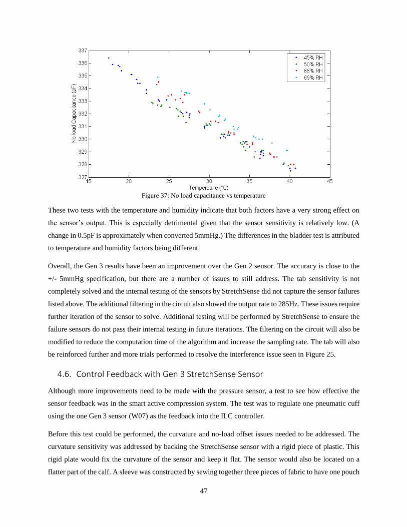
47
Figure 37: No load capacitance vs temperature
These two tests with the temperature and humidity indicate that both factors have a very strong effect on
the sensor’s output. This is especially detrimental given that the sensor sensitivity is relatively low. (A
change in 0.5pF is approximately when converted 5mmHg.) The differences in the bladder test is attributed
to temperature and humidity factors being different.
Overall, the Gen 3 results have been an improvement over the Gen 2 sensor. The accuracy is close to the
+/- 5mmHg specification, but there are a number of issues to still address. The tab sensitivity is not
completely solved and the internal testing of the sensors by StretchSense did not capture the sensor failures
listed above. The additional filtering in the circuit also slowed the output rate to 285Hz. These issues require
further iteration of the sensor to solve. Additional testing will be performed by StretchSense to ensure the
failure sensors do not pass their internal testing in future iterations. The filtering on the circuit will also be
modified to reduce the computation time of the algorithm and increase the sampling rate. The tab will also
be reinforced further and more trials performed to resolve the interference issue seen in Figure 25.
4.6. Control Feedback with Gen 3 StretchSense Sensor
Although more improvements need to be made with the pressure sensor, a test to see how effective the
sensor feedback was in the smart active compression system. The test was to regulate one pneumatic cuff
using the one Gen 3 sensor (W07) as the feedback into the ILC controller.
Before this test could be performed, the curvature and no-load offset issues needed to be addressed. The
curvature sensitivity was addressed by backing the StretchSense sensor with a rigid piece of plastic. This
rigid plate would fix the curvature of the sensor and keep it flat. The sensor would also be located on a
flatter part of the calf. A sleeve was constructed by sewing together three pieces of fabric to have one pouch

48
for the sensor and one pouch for the plate to be slip into. This sleeve was then taped to the leg loosely so
that the sensor was not experiencing any load. The no-load offset was mitigated by adding a thermistor to
measure the temperature near the sensor. A linear correction factor of -0.38pF/°C was added to the
capacitance measurement to compensate for the thermal effects. The effect of humidity was addressed by
using the capacitance measurement when the sensor was loosely taped to the leg as the zero pressure. The
assumption was that the humidity would remain fairly constant for the short period of time that the test was
run.
The conversion of the capacitance to pressure used the following equation:
𝑃 = 𝑘𝑠𝑒𝑛𝑠𝑖𝑡𝑖𝑣𝑖𝑡𝑦 ∗ (𝐶 − 𝐶𝑧𝑒𝑟𝑜 + 𝑘𝑡ℎ𝑒𝑟𝑚𝑎𝑙 𝑐𝑜𝑒𝑓𝑓𝑖𝑐𝑖𝑒𝑛𝑡 ∗ (𝑇 − 𝑇𝑧𝑒𝑟𝑜)) (7)
where 𝑃 is the pressure prediction (mmHg), 𝑘𝑠𝑒𝑛𝑠𝑖𝑡𝑖𝑣𝑖𝑡𝑦 is the sensor sensitivity (mmHg/pF), 𝐶 is the
capacitance of the sensor (pF), 𝐶𝑧𝑒𝑟𝑜 is the capacitance measured when the sensor is zeroed and has no-
load (pF), 𝑘𝑡ℎ𝑒𝑟𝑚𝑎𝑙 𝑐𝑜𝑒𝑓𝑓𝑖𝑐𝑖𝑒𝑛𝑡 is the thermal coefficient of the sensor (pF/°C), 𝑇 is the temperature
measured by the thermistor (°C), and 𝑇𝑧𝑒𝑟𝑜 is the temperature measured when the sensor is zeroed and has
no-load (°C).
The pressure measurement from Eqn 7 was used to replace one of the inputs from the PicoPress sensor to
the ILC controller. The design of the LabVIEW program allowed a simple change in code to facilitate this
new sensor input. The result was very similar to the previous setup with the PicoPress as feedback. Figure
38 shows the ILC controller operating with the Gen 3 sensor as feedback responding to a step change in
target pressure from 50 to 60mmHg. It was able to make the step change in 4 iterations. This is expected
since the ILC controller should work regardless of the type of sensor input; as long as the sensor information
is accurate, the controller will operate the same before.
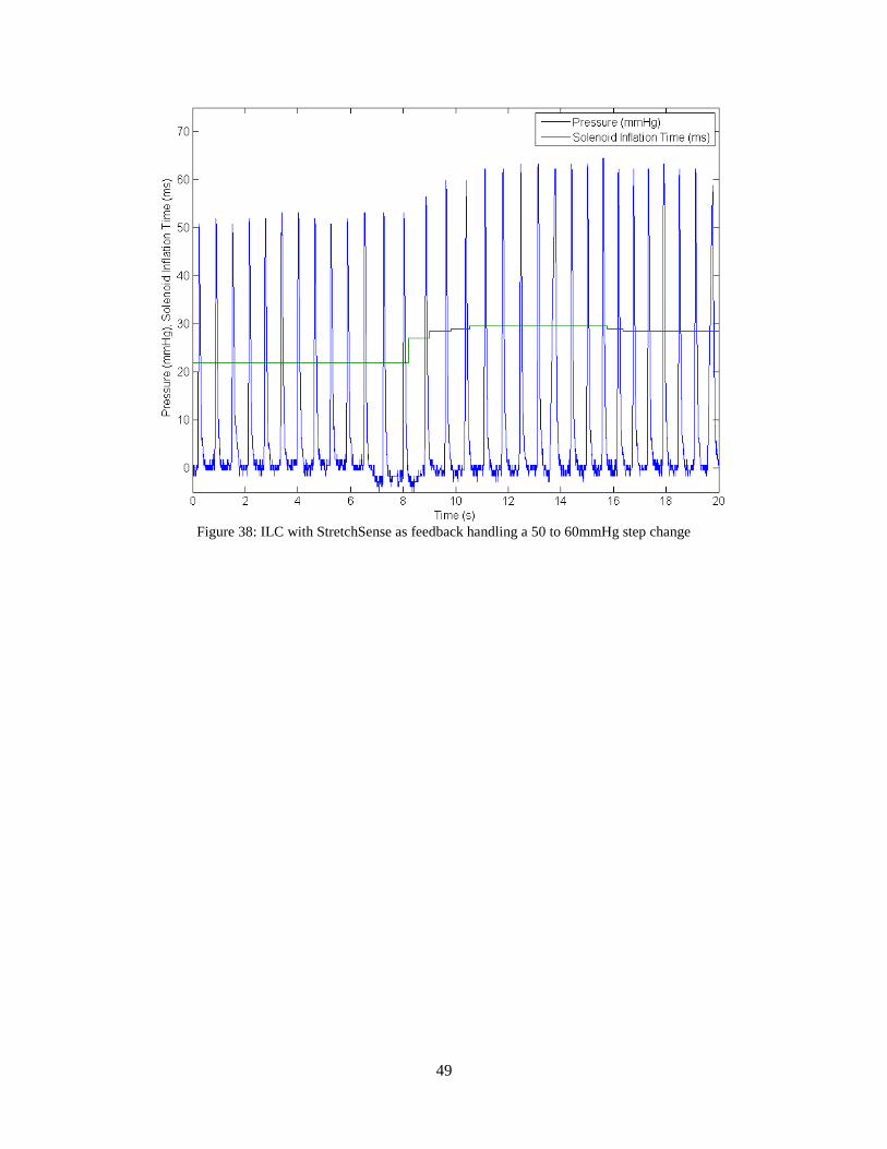
49
Figure 38: ILC with StretchSense as feedback handling a 50 to 60mmHg step change

50
Chapter 5 Conclusions and Future Work
5.1. Conclusions
The goal of this research was to develop a control system to consistently apply an intermittent pressure
around a leg for a study in active compression on the lower extremities. The control system consisted of a
new timing algorithm to apply compression at the end the flow of a blood pulse in the leg. The timing
algorithm uses an ECG to detect the heartbeat and a delay that accounts for pulse wave delay, and a heel
switch that prevents the compression from operating when the calf muscles are contracted. The control
system also includes an iterative learning controller for regulating the amount of pressure applied to the leg.
The feedback control was originally using a custom PicoPress system with a multiplexer, but difficulties
with the accuracy and size of the system warranted a new sensing system. This new sensing system used a
capacitive sensing modality developed by StretchSense that has been evaluated.
Based on the testing performed in this research, the follow conclusions are presented:
1. Multiplexing of PicoPress sensors is not feasible
The PicoPress sensor requires operation in a closed system. By sharing one pressure transducer
across multiple PicoPress bladders, there must be a small volume of air being shared. This causes
pressurized air to move between bladders and so the closed system requirement is broken.
2. R-peak detection with 3-point thresholding is reliable for healthy subjects
A method of detecting the R-peak was needed to synchronize the compression with the heartbeat.
The custom algorithm developed in Section 3.2.2 was able to detect 100% of R-peaks in the two
test samples and during the testing of the active compression system. One caveat is that the subjects
tested were all healthy adults.
3. An ILC controller is well suited for regulating a pneumatic compression system
The ILC controller developed for this active compression system successfully regulated the
pressure being applied to the leg under varied conditions. The strength of the controller is in its
adaptability and continuous correction of the actuator. The ILC controller was able to meet step
changes in the target pressure in an average of 4.2 iteration.
4. Pressure sensing for compression garments is an on-going challenge

51
The difficulties of discovering a tactile pressure sensor for the pressure range, the sampling
frequency, size, and accuracy required is demonstrated. Although a capacitive sensing modality
seemed to be the most promising technology, trade-offs were made that compromised the ideal
specifications originally defined for this application.
5. Capacitive sensors shown to be viable as pressure sensing technology in compression garments
The capacitive StretchSense sensor still does not meet the relaxed specifications. However, the Gen
3 sensor results are very close to the required specifications and future iterations will attempt to
resolve the remaining issues. The Gen 3 sensor was successfully used in a short test that read its
data as the feedback into the ILC controller.
6. Curvature has a very significant effect on capacitive pressure sensors
The curvature of the sensor greatly affects its output. Without a method controlling this variable,
the pressure predicted can be skewed by 30mmHg or more. A rigid backing and sleeve was made
to keep the sensor flat when in use.
5.2. Future Work
This thesis presents a functioning active compression system. The system can be used as a basis for future
work and continued improvements. A few items that can be improved upon are:
Continued improvements to the StretchSense sensor. The Gen 3 sensor did not meet the accuracy
and sampling rate required. Further iterations of the sensor can attempt to address those
deficiencies.
Improve sensitivity of capacitance measurement. The low sensor sensitivity and measurement
resolution of 0.1pF mean that the minimum pressure resolution is about 1mmHg. Improving the
pressure resolution may help improve sensor accuracy because it can potentially be less sensitive
to noise and thermal changes. Efforts should be made to increase sensor sensitivity.
Longer studies necessary to verify stability of StretchSense sensors. The temperature and humidity
effects were addressed with simple measures that worked for the tests with the ILC controller. Tests
for a longer period of time should be performed to ensure the results are consistent.
Making the compression system more mobile. The current pneumatic compression system is not
portable and is difficult to use in studies that require the subject to walk or exercise. A more portable
system would be beneficial.

52
References
[1] Guyton, A. C., & Jones, C. E. (1973). Central venous pressure: physiological significance
and clinical implications. American heart journal, 86(4), 431.
[2] Calne, S. (Ed.). (2003). Understanding compression therapy. London, UK: Medical
Education Partnership.
[3] Morris, R. J., & Woodcock, J. P. (2004). Evidence-based compression: prevention of
stasis and deep vein thrombosis. Annals of surgery, 239(2), 162.
[4] Troynikov, O., Ashayeri, E., Burton, M., Subic, A., Alam, F., & Marteau, S. (2010).
Factors influencing the effectiveness of compression garments used in sports. Procedia
Engineering, 2(2), 2823-2829.
[5] Wardiningsih, W., Troynikov, O., Molotnikov, A., & Estrin, Y. (2013). Influence of
Protective Pad Integrated into Sport Compression Garments on their Pressure Delivery to
Athlete's Lower Limbs. Procedia Engineering, 60, 170-175.
[6] Ali, A., Creasy, R. H., & Edge, J. A. (2011). The effect of graduated compression
stockings on running performance. The Journal of Strength & Conditioning Research,
25(5), 1385-1392.
[7] Michael, J. S., Dogramaci, S. N., Steel, K. A., & Graham, K. S. (2014). What is the effect
of compression garments on a balance task in female athletes?. Gait & posture, 39(2),
804-809.
[8] Thiriet, M. (2014). Anatomy and Physiology of the Circulatory and Ventilatory Systems.
New York: Springer.
[9] Noordergraaf, A. (2011). Blood in Motion. Springer Science & Business Media.
[10] Laboratoires URGO. (2009). Retrieved November 10, 2015, from
http://www.urgo.co.uk/260-the-venous-system-within-the-cardiovascular-system
[11] Thiriet, M. (2014). Anatomy and Physiology of the Circulatory and Ventilatory Systems.
New York: Springer.
[12] Human Heart. (2012). Retrieved November 10, 2015, from http://www.infohow.org/wp-
content/uploads/2012/11/Human-Heart.jpg
[13] Barill, T. (2003). An ECG Primer.
[14] Cardiac Cycle. (2015). Retrieved November 10, 2015, from
https://cnx.org/contents/22c3f969-ab9d-4df0-8baf-5b1a99372fac@3/Cardiac-Cycle
[15] Blood Flow, Blood Pressure, and Resistance. (2015). Retrieved November 10, 2015, from
http://cnx.org/contents/[email protected]:133/Blood-Flow-
Blood-Pressure-and-
[16] Lord, R. S., & Hamilton, D. (2004). Graduated compression stockings (20− 30 mmHG)
do not compress leg veins in the standing position. ANZ journal of surgery, 74(7), 581-
585.
[17] Dai, G., Gertler, J. P., & Kamm, R. D. (1999). The effects of external compression on
venous blood flow and tissue deformation in the lower leg. Journal of biomechanical
engineering, 121(6), 557-564.
[18] Partsch, B., & Partsch, H. (2005). Calf compression pressure required to achieve venous
closure from supine to standing positions. Journal of vascular surgery, 42(4), 734-738.

53
[19] Born, D. P., Holmberg, H. C., Goernert, F., & Sperlich, B. (2014). A novel compression
garment with adhesive silicone stripes improves repeated sprint performance–a multi-
experimental approach on the underlying mechanisms. BMC sports science, medicine and
rehabilitation, 6(1), 21.
[20] Book, J. (2014). Investigating the Impact of External Passive Compression on Central
and Peripheral Hemodynamics (Master’s thesis). University of Waterloo, Waterloo, ON.
[21] Lurie, F., Scott, V., Yoon, H. C., & Kistner, R. L. (2008). On the mechanism of action of
pneumatic compression devices: Combined magnetic resonance imaging and duplex
ultrasound investigation. Journal of vascular surgery, 48(4), 1000-1006.
[22] Sheldon, R. D., Roseguini, B. T., Laughlin, M. H., & Newcomer, S. C. (2013). New
insights into the physiologic basis for intermittent pneumatic limb compression as a
therapeutic strategy for peripheral artery disease. Journal of vascular surgery, 58(6),
1688-1696.
[23] Sheldon, R. D., Roseguini, B. T., Thyfault, J. P., Crist, B. D., Laughlin, M. H., &
Newcomer, S. C. (2012). Acute impact of intermittent pneumatic leg compression
frequency on limb hemodynamics, vascular function, and skeletal muscle gene expression
in humans. Journal of Applied Physiology, 112(12), 2099-2109.
[24] Tochikubo, O., Ri, S., & Kura, N. (2006). Effects of pulse-synchronized massage with air
cuffs on peripheral blood flow and autonomic nervous system. Circulation Journal,
70(9), 1159-1163.
[25] Yousef, H., Boukallel, M., & Althoefer, K. (2011). Tactile sensing for dexterous in-hand
manipulation in robotics—A review. Sensors and Actuators A: physical, 167(2), 171-187.
[26] Tiwana, M. I., Redmond, S. J., & Lovell, N. H. (2012). A review of tactile sensing
technologies with applications in biomedical engineering. Sensors and Actuators A:
physical, 179, 17-31.
[27] Partsch, H., Clark, M., Bassez, S., BENIGNI, J. P., Becker, F., Blazek, V., ... &
Neumann, M. (2006). Measurement of lower leg compression in vivo: recommendations
for the performance of measurements of interface pressure and stiffness. Dermatologic
surgery, 32(2), 224-233.
[28] Flaud, P., Bassez, S., & COUNORD, J. L. (2010). Comparative in vitro study of three
interface pressure sensors used to evaluate medical compression hosiery. Dermatologic
Surgery, 36(12), 1930-1940.
[29] Pressure Measuring Device MST MK IV. (2015). Retrieved November 2, 2015, from
http://www.salzmann-group.ch/4/400/3/130/130/0/index.html
[30] Kikuhime. (2014). Retrieved November 2, 2015, from
http://www.advancis.co.uk/products/other-products/kikuhime
[31] Pico Press. (2014). Retrieved November 3, 2015, from http://www.microlabitalia.it/case-
history.php?azione=show&url=pico-press
[32] Burke, M., Murphy, B., & Geraghty, D. (2014, November). Measurement of sub-bandage
pressure during venous compression therapy using flexible force sensors. In SENSORS,
2014 IEEE (pp. 1623-1626). IEEE.
[33] FlexiForce Load/Force Sensors and Systems. (n.d.). Retrieved November 2, 2015, from
https://www.tekscan.com/flexiforce-load-force-sensors-and-systems
[34] FSR 402. (2015). Retrieved November 2, 2015, from
http://www.interlinkelectronics.com/FSR402.php

54
[35] Ferguson-Pell, M., Hagisawa, S., & Bain, D. (2000). Evaluation of a sensor for low
interface pressure applications. Medical engineering & physics, 22(9), 657-663.
[36] Najarian, S., Dargahi, J., & Mehrizi, A. (2009). Artificial tactile sensing in biomedical
engineering. New York: McGraw Hill Professional.
[37] Siegel, D. M., Drucker, S. M., & Garabieta, I. (1987, March). Performance analysis of a
tactile sensor. In Proc. IEEE Conf. on Robotics and Automation (Vol. 3, pp. 1493-1499).
[38] Ko, W. H., & Wang, Q. (1999). Touch mode capacitive pressure sensors. Sensors and
Actuators A: Physical, 75(3), 242-251.
[39] (C. Prince, personal communication, September 2013).
[40] (C. Prince, personal communication, August 2014).
[41] Sadhukhan, D., & Mitra, M. (2012). R-Peak detection algorithm for ECG using double
difference and RR interval processing. Procedia Technology, 4, 873-877.
[42] Chen, C. K., & Hwang, J. (2005). Iterative learning control for position tracking of a
pneumatic actuated X–Y table. Control Engineering Practice, 13(12), 1455-1461.
[43] 5 Port Solenoid Valve. (2011). Retrieved November 20, 2015, from
http://www.smcpneumatics.com/pdfs/VQZ_5PT.pdf
[44] StretchSense. (2015). Retrieved November 2, 2015, from http://stretchsense.com/
[45] Silicone Rubber. (2015). Retrieved November 26, 2015, from
http://www.azom.com/properties.aspx?ArticleID=920
[46] Hibbeler, R. (2011). Mechanics of materials (8th ed.). Boston: Prentice Hall.