web appendices for “the technology of skill...
TRANSCRIPT

Web Appendices for“The Technology of Skill Formation”
Flavio Cunha and James Heckman
Article published in American Economic Review 97(2), May 2007
Contents
A Deriving the Technology of Skill Formation from its Primitives 2
B Comparing the Technology of Skill Formation to the Ben-PorathModel 12B.1 The General Technology of Skill Formation . . . . . . . . . . . 12B.2 Relationship with the Ben-Porath (1967) Model . . . . . . . . . 14
C An OLG/Complete Markets Model 16
D Program Definitions, Tables and Figures 20
1

A Deriving the Technology of Skill Formationfrom its Primitives
A Model of Skill Formation
In the models presented in this section of the appendix and in CHLM,parents make decisions about their children. We ignore how the parentsget to be who they are and the decisions of the children about their ownchildren. Appendix C develops a generationally consistent model.
Suppose that there are two periods in a child’s life, “1” and “2”, beforethe child becomes an adult. Adulthood comprises distinct third and fourthperiods. The child works for two periods after the two periods of childhood.Models based on the analysis of Becker and Tomes (1986) assume only oneperiod of childhood. We assume that there are two kinds of skills: θC andθN.For example, θC can be thought of as cognitive skill and θN as noncognitiveskill. Our treatment of ability is in contrast to the view of the traditionalliterature on human capital formation that views IQ as innate ability. In ouranalysis, IQ is just another skill. What differentiates IQ from other cognitiveand noncognitive skills is that IQ is subject to accumulation during criticalperiods. That is, parental and social interventions can increase the IQ of thechild, but they can do so successfully only for a limited time.
Let Ikt denote parental investments in child skill k at period t, k = C,N and
t = 1, 2. Let h′ be the level of human capital as the child starts adulthood.It depends on both components of (θC
2 , θN2 ). The parents fully control the
investment of the child. A richer model incorporates, among other features,investment decisions of the child as influenced by the parent through pref-erence formation processes (see Carneiro, Cunha, and Heckman, 2003, andCunha and Heckman, 2007a).
We first describe how skills evolve over time. Assume that each agentis born with initial conditions θ1 =
(θC
1 , θN1
). These can be determined by
parental environments. At each stage t let θt =(θC
t , θNt
)denote the vector of
skill or ability stocks. The technology of production of skill k at period t is
θkt+1 = f k
t
(θt, Ik
t
), (A-1)
for k = C,N and t = 1, 2. We assume that f kt is twice continuously differ-
entiable, increasing and concave. In this model, stocks of both skills andabilities produce next period skills and the productivity of investments.Cognitive skills can promote the formation of noncognitive skills and vice
2

versa.Let θC
3 , θN3 denote the level of skills when adult. We define adult human
capital h′ of the child as a combination of different adult skills:
h′ = g(θC
3 , θN3
). (A-2)
The function g is assumed to be continuously differentiable and increasingin
(θC
3 , θN3
). This model assumes that there is no comparative advantage in
the labor market or in life itself.1
To fix ideas, consider the following specialization of our model. Ignorethe effect of initial conditions and assume that first period skills are just dueto first period investment:
θC2 = f C
1
(θ1, IC
1
)= IC
1
andθN
2 = f C1
(θ1, IC
1
)= IN
1 ,
where IC1 and IN
1 are scalars. For the second period technologies, assume aCES structure:
θC3 = f C
2
(θ2, IC
2
)(A-3)
={γ1
(θC
2
)α+ γ2
(θN
2
)α+
(1 − γ1 − γ2
) (IC2
)α} 1α where
1 ≥ γ1 ≥ 0,1 ≥ γ2 ≥ 0,1 ≥ 1 − γ1 − γ2 ≥ 0,
and
θN3 = f N
2
(θ2, IN
2
)(A-4)
={η1
(θC
2
)ν+ η2
(θN
2
)ν+
(1 − η1 − η2
) (IN2
)ν} 1ν where
1 ≥ η1 ≥ 0,1 ≥ η2 ≥ 0,1 ≥ 1 − η1 − η2 ≥ 0,
where 11−α is the elasticity of substitution in the inputs producing θC
3 and 11−ν
is the elasticity of substitution of inputs in producing θN3 where α ∈ (−∞, 1]
and ν ∈ (−∞, 1]. Notice that IN2 and IC
2 are direct complements with (θC2 , θ
N2 )
1Thus we rule out one potentially important avenue of compensation that agents canspecialize in tasks that do not require the skills in which they are deficient. In CHLM webriefly consider a more general task function that captures the notion that different tasksrequire different combinations of skills and abilities.
3

irrespective of the substitution parameters α and ν, except in limiting cases.The CES technology is well known and has convenient properties. It
imposes direct complementarity even though inputs may be more or lesssubstitutable depending on α or ν. We distinguish between direct comple-mentarity (positive cross partials) and CES-substitution/complementarity.Focusing on the technology for producing θC
3 , when α = 1, the inputs areperfect substitutes in the intuitive use of that term (the elasticity of substi-tution is infinite). The inputs θC
2 , θN2 and IC
2 can be ordered by their relativeproductivity in producing θC
3 . The higher γ1 and γ2, the higher the produc-tivity of θC
2 and θN2 respectively. When α = −∞, the elasticity of substitution
is zero. All inputs are required in the same proportion to produce a givenlevel of output so there are no possibilities for technical substitution, and
θC3 = min
{θC
2 , θN2 , I
C2
}.
In this technology, early investments are a bottleneck for later investment.Compensation for adverse early environments through late investments isimpossible.
The evidence from numerous studies reviewed in the text and in CHLMcited shows that IQ is no longer malleable after ages 8-10. Taken at facevalue, this implies that if θC is IQ, for all values of IC
2 , θC3 = θ
C2 . Period 1 is a
critical period for IQ but not necessarily for other skills and abilities. Moregenerally, period 1 is a critical period if
∂θCt+1
∂ICt
= 0 for t > 1.
For parameterization (A-3), this is obtained by imposing γ1+ γ2 = 1.The evidence on adolescent interventions surveyed in CHLM shows
substantial positive results for such interventions on noncognitive skills (θN3 )
and at most modest gains for cognitive skills. Technologies (A-3) and (A-4)can rationalize this pattern. Since the populations targeted by adolescentintervention studies tend to come from families with poor backgrounds,we would expect IC
1 and IN1 to be below average. Thus, θC
2 and θN2 will be
below average. Adolescent interventions make IC2 and IN
2 relatively large forthe treatment group in comparison to the control group in the interventionexperiments. At stage 2, θC
3 (cognitive ability) is essentially the same inthe control and treatment groups, while θN
3 (noncognitive ability) is higherfor the treated group. Large values of
(γ1 + γ2
)(associated with a small
coefficient on IC2 ) or small values of
(η1 + η2
)(so the coefficient on IN
2 is
4

large) and high values of α and ν can produce this pattern. Another casethat rationalizes the evidence is when α → −∞ and ν = 1. Under theseconditions,
θC3 = min
{θC
2 , θN2 , I
C2
}, (A-5)
whileθN
3 = η1θC2 + η2θ
N2 +
(1 − η1 − η2
)IN2 . (A-6)
The attainable period 2 stock of cognitive skill(θC
3
)is limited by the mini-
mum value ofθC2 , θ
N2 , I
C2 . In this case, any level of investment in period 2 such
that IC2 > min
{θC
2 , θN2
}is ineffective in incrementing the stock of cognitive
skills. Period 1 is a bottleneck period. Unless sufficient skill investments aremade in θC in period 1, it is not possible to raise skill θC in period 2. Thisphenomenon does not appear in the production of the noncognitive skill,provided that
(1 − η1 − η2
)> 0. More generally, the higher ν and the larger(
1 − η1 − η2), the more productive is investment IN
2 in producing θN2 .
To complete the CES example, assume that adult human capital h′ is aCES function of the two skills accumulated at stage two:
h′ ={τ(θC
3
)φ+ (1 − τ)
(θN
3
)φ} ρφ
, (A-7)
where ρ ∈ (0, 1), τ ∈ [0, 1], and φ ∈ (−∞, 1]. In this parameterization, 11−φ is
the elasticity of substitution across different skills in the production of adulthuman capital. Equation (A-7) reminds us that the market, or life in gen-eral, requires use of multiple skills. Being smart isn’t the sole determinantof success. In general, different tasks require both skills in different pro-portions. One way to remedy early skill deficits is to make compensatoryinvestments. Another way is to motivate people from disadvantaged envi-ronments to pursue tasks that do not require the skill that deprived earlyenvironments do not produce. A richer theory would account for this choiceof tasks and its implications for remediation.2 For the sake of simplifyingour argument, we work with equation (A-7) that captures the notion thatskills can trade off against each other in producing effective people. Highlymotivated, but not very bright, people may be just as effective as bright butunmotivated people. That is one of the lessons from the GED program. (SeeHeckman and Rubinstein, 2001, and Heckman, Stixrud, and Urzua, 2006.)
The analysis is simplified by assuming that investments are general in
2See the appendix in CHLM.
5
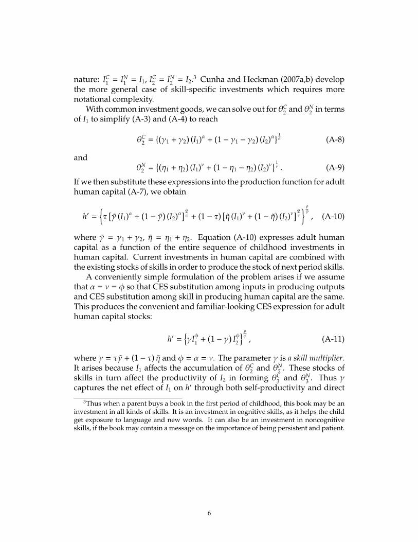
nature: IC1 = IN
1 = I1, IC2 = IN
2 = I2.3 Cunha and Heckman (2007a,b) developthe more general case of skill-specific investments which requires morenotational complexity.
With common investment goods, we can solve out for θC2 and θN
2 in termsof I1 to simplify (A-3) and (A-4) to reach
θC2 =
{(γ1 + γ2
)(I1)α +
(1 − γ1 − γ2
)(I2)α
} 1α (A-8)
andθN
2 ={(η1 + η2
)(I1)ν +
(1 − η1 − η2
)(I2)ν
} 1ν . (A-9)
If we then substitute these expressions into the production function for adulthuman capital (A-7), we obtain
h′ ={τ[γ̃ (I1)α +
(1 − γ̃
)(I2)α
] φα + (1 − τ)
[η̃ (I1)ν +
(1 − η̃
)(I2)ν
] φν
} ρφ
, (A-10)
where γ̃ = γ1 + γ2, η̃ = η1 + η2. Equation (A-10) expresses adult humancapital as a function of the entire sequence of childhood investments inhuman capital. Current investments in human capital are combined withthe existing stocks of skills in order to produce the stock of next period skills.
A conveniently simple formulation of the problem arises if we assumethat α = ν = φ so that CES substitution among inputs in producing outputsand CES substitution among skill in producing human capital are the same.This produces the convenient and familiar-looking CES expression for adulthuman capital stocks:
h′ ={γIφ1 +
(1 − γ
)Iφ2
} ρφ, (A-11)
where γ = τγ̃ + (1 − τ) η̃ and φ = α = ν. The parameter γ is a skill multiplier.It arises because I1 affects the accumulation of θC
2 and θN2 . These stocks of
skills in turn affect the productivity of I2 in forming θC3 and θN
3 . Thus γcaptures the net effect of I1 on h′ through both self-productivity and direct
3Thus when a parent buys a book in the first period of childhood, this book may be aninvestment in all kinds of skills. It is an investment in cognitive skills, as it helps the childget exposure to language and new words. It can also be an investment in noncognitiveskills, if the book may contain a message on the importance of being persistent and patient.
6

complementarity.4 11−φ is a measure of how easy it is to substitute between I1
and I2 where the substitution arises from both the task performance (humancapital) function in equation (A-7) and the technology of skill formation.Within the CES technology, φ is a measure of the ease of substitution ofinputs. In this analytically convenient case, the parameter φ plays a dualrole. First, it informs us how easily one can substitute across differentskills in order to produce one unit of adult human capital h′. Second, it alsorepresents the degree of complementarity (or substitutability) between earlyand late investments in producing skills. In this second role, the parameterφ dictates how easy it is to compensate for low levels of stage 1 skills inproducing late skills.
In principle, compensation can come through two channels: (i) throughskill investment or (ii) through choice of market activities, substitutingdeficits in one skill by the relative abundance in the other through choiceof tasks. We do not develop the second channel of compensation in thisappendix, deferring it to later work. It is discussed in Carneiro, Cunha, andHeckman (2003).
When φ is small, low levels of early investment I1 are not easily reme-diated by later investment I2 in producing human capital. The other faceof CES complementarity is that when φ is small, high early investmentsshould be followed with high late investments. In the extreme case whenφ → −∞, (A-11) converges to h′ = (min {I1, I2})
ρ. We analyzed this case inCHLM. The Leontief case contrasts sharply with the case of perfect CESsubstitutes, which arises when φ = 1: h′ =
[γI1 +
(1 − γ
)I2]ρ. When we
impose the further restriction that γ = 12 , we generate the model that is im-
plicitly assumed in the existing literature on human capital investments thatcollapses childhood into a single period. In this special case, only the total
4Direct complementarity between I1 and I2 arises if
∂2h∂I1∂I2
> 0.
As long as ρ > φ, I1 and I2 are direct complements, because
sign(∂2h∂I1∂I2
)= sign(ρ − φ).
This definition of complementarity is to be distinguished from the notion based on theelasticity of substitution between I1 and I2, which is 1
1−φ . When φ < 0, I1 and I2 aresometimes called complements. When φ > 0, I1 and I2 are sometimes called substitutes.When ρ = 1, I1 and I2 are always direct complements, but if 1 > φ > 0, they are CESsubstitutes.
7

amount of human capital investments, regardless of how it is distributedacross childhood periods, determines adult human capital. In the case ofperfect CES substitutes, it is possible in a physical productivity sense tocompensate for early investment deficits by later investments, although itmay not be economically efficient to do so.
When ρ = 1, we can rewrite (A-11) as
h′ = I1
{γ +
(1 − γ
)ωφ
} 1φ,
where ω = I2/I1. Fixing I1 (early investment), an increase in ω is the same asan increase in I2. The marginal productivity of late investment is
∂h′
∂ω=
(1 − γ
)I1
{γ +
(1 − γ
)ωφ
} 1−φφωφ−1.
For ω > 1 and γ < 1, marginal productivity is increasing in φ and(1 − γ
).
Thus, provided that late investments are greater than earlier investments,the more substitutable I2 is with I1 (the higher φ) and the lower the skillmultiplier γ, the more productive are late investments. Figure A1 graphsthe isoquants for ∂h′
∂ω when ω = 2. It shows that a high φ trades off with ahigh γ. As
(φ, 1 − γ
)increases along a ray, ∂h′
∂ω increases. For a fixed skillmultiplier γ, the higher φ, the higher the marginal productivity of secondperiod investment.
If, however, ω < 1 as in Figure A2, then ∂h′∂ω could be decreasing as(
φ, 1 − γ)
increases along a ray and the trade-off between φ and(1 − γ
)along a
(∂h′∂ω , ω
)isoquant is reversed. If I1 is large relative to I2 (i.e., ω < 1),
for a fixed γ the marginal product of I2 is decreasing in φ. More CES com-plementarity implies greater productivity (see Figure A2).5 The empiricallyrelevant case for the analysis of investment in disadvantaged children isω > 1 as shown in Figure C3, so greater CES-substitutability and a smallerskill multiplier produce a higher marginal productivity of remedial secondperiod investment.
5One can show that at sufficiently low values ofφ, the marginal productivity is no longerincreasing in φ.
8

0.2 0.3 0.4 0.5 0.6 0.7 0.8-3
-2. 5
-2
-1. 5
-1
-0. 5
0
0.5
1
Skill Multiplier (γ)
0.098918
0.098918
0.19784
0.19784
0.29676
0.29676
0.39567
7
0.49459
9351
Figure A1
when I2/I1 = 2.
The indifference curves of the marginal productivity of theratio of late to early investments as a function of φ and γ
Define ω = I2I1, the ratio of late to early investments in human capital. From the homogeneity of degree one
we can rewrite the technology as:
h = I1£γ + (1− γ)ωφ
¤ 1φ .
The marginal product of the ratio of late to early investment, ω, holding early investment constant, is
∂h
∂ω= (1− γ) I1
£γ + (1− γ)ωφ
¤ 1−φφ ωφ−1
This figure displays the indifference curves of ∂h∂ω when ω = 0.5. Each indifference curve shows the corresponding
level of ∂h∂ω . Note that for a given value of γ the value of the function tends to decrease as we increase φ. The
function also increases as we decrease γ.
2
9

0.2 0.3 0.4 0.5 0.6 0.7 0.8-3
-2. 5
-2
-1. 5
-1
0. 5
0
0.5
1
Skill Multiplier (γ)
0.3
0.5046
0.63492
0.6
0.76525
0.76525
0.89557
0.89557
0.89
1.02591.0259
Figure A2The indifference curves of the marginal productivity of the
ratio of late to early investments as a function of φ and γwhen I2/I1 = 1/2.
Consider the CES specification for the technology of human capital formation:
h =hγIφ1 + (1− γ) Iφ2
i 1φ
Define ω = I2I1, the ratio of late to early investments in human capital. From the homogeneity of degree one we
can rewrite the technology as:
h = I1£γ + (1− γ)ωφ
¤ 1φ .
The marginal product of the ratio of late to early investment, ω, holding early investment constant, is
∂h
∂ω= (1− γ) I1
£γ + (1− γ)ωφ
¤ 1−φφ ωφ−1
This figure displays the indifference curves of ∂h∂ω when ω = 0.5. Each indifference curve shows the corresponding
level of ∂h∂ω . Note that for a given value of γ the value of the function tends to decrease as we increase φ. However,
the function may not be monotonic with respect to γ.
1
10

����� 7� The Ratio of Optimal Early and Late Investments ����Under Di�erent Assumptions About the Skill Formation Technology
Low Self-Productivity: � � ���������� High Self-Productivity: � � �����
�����
High Degree of Complementarity: � � � ����� � as �� �� ��
��� � as �� ��
Low Degree of Complementarity: � � � � � ����� � as �� � ��
���� as �� �
����� This table summarizes the behavior of the ratio of optimal early to late investments according to four cases: �� and �� havehigh complementarity, but self-productivity is low; �� and �� have both high complementarity and self-productivity; �� and �� havelow complementarity and self-productivity; and �� and �� have low complementarity, but high self-productivity. When �� and ��exhibit high complementary, complementarity dominates and is a force towards equal distribution of investments between earlyand late periods. Consequently, self-productivity plays a limited role in determining the ratio ��
��(row 1). On the other hand, when
��and �� exhibit a low degree of complementarity, self-productivity tends to concentrate investments in the ���� period ifself-productivity is low, but in the ���� period if it is high (row 2).
11

B Comparing the Technology of Skill Formationto the Ben-Porath Model
B.1 The General Technology of Skill Formation
Let θt be a L × 1 vector of skills or abilities at stage t. Included are purecognitive abilities (e.g. IQ) as well as noncognitive abilities (time preference,self control, patience, judgment). The notation is sufficiently flexible toinclude acquired skills like general education or a specific skill. Agents startout life with vector θ1 of skills (abilities). The θ1 are produced by genes andin utero environments which are known to affect child outcomes (see, e.g.,the essays in Keating and Hertzman, 1999).
Let It be a K × 1 vector of investments at stage t. These include all inputsinvested in the child including parental and social inputs. The technologyof skill formation can be written as
θt+1 = ft (θt, It)
where ft is a stage-t function mapping skill (ability) levels and investmentat stage t into skill (ability) levels at the end of the period. For simplicitywe assume that ft is twice continuously differentiable in its arguments. Itsdomain of definition is the same for all inputs. The inputs may be differentat different stages of the life cycle, so the inputs in It may be different fromthe inputs at period τ different from t.
Universal self-productivity at stage t is defined as
∂θt+1
∂θt=∂ ft
∂θt> 0.
In the general case this is a L × L matrix. More generally, some componentsof this matrix may be zero at all stages while other components may alwaysbe positive. In principle, some skills could have negative effects in someperiods. At some stages, some components may be zero while at otherstages they may be positive.
Universal direct complementarity at stage t is defined by the L×K matrix:
∂2θt+1
∂θt∂I′t> 0.
Higher levels of θt raise the productivity of It. Alternatively, higher levels of
12

It raise the productivity of θt. Again, in the general case, some componentsat some or all stages may have zero effects, and some may have negativeeffects. They can switch signs across stages.
This notation is sufficiently general to allow for the possibility that somecomponents of skill are produced only at certain critical periods. Period t iscritical for skill (ability) j if
∂θt+1, j
∂It, 0,
for some levels of θt, It = it, but
∂θt+k+1, j
∂It+k= 0, k > 0,
for all levels of θt, It = it.Sensitive periods might be defined as those periods where, at the same
level of input θt, It, the ∂θt+1∂It
are high. More formally, letting θt = ϑ, It = i, t isa sensitive period for skill (or ability) j if
∂θt+k+1, j
∂It+k
∣∣∣∣∣∣θt+k=ϑ,It+k=i
<∂θt+1, j
∂It
∣∣∣∣∣∣θt=ϑ,It=i
, for k , 0.
Clearly there may be multiple sensitive periods, and there may be sensitivitywith respect to one input that is not true of other inputs.
An alternative definition of critical and sensitive periods works witha version of the technology that solves out θt+1, j as a function of laggedinvestments and initial conditions θ1 = θ1:
θt+1, j =Mt, j (It, It−1, . . . , I1, θ1) , j = 1, . . . , J.
Stage t∗ is a critical period for θt+1, j if investments are productive at t∗ but notat any other stage k , t∗. Formally,
∂θt+1, j
∂Ik=∂Mt, j (It, It−1, . . . , I1, θ1)
∂Ik≡ 0, k , t∗, j = 1, . . . , J,
for all θ1, I1, . . . , It, but
∂θt+1, j
∂It∗=∂Mt, j (It, It−1, . . . , I1, θ0)
∂It∗> 0, j = 1, . . . , J,
for some θ1, I1, . . . , It.
13

Stage t∗ is a sensitive period for θt+1, j if at the same level of inputs, invest-ment is more productive at stage t∗ than at stage t. Formally, t∗ is a sensitiveperiod for θt+1, j if for k , t∗,
∂θt+1, j
∂Ik
∣∣∣∣∣∣θ1=θ1,Ik=ik,k=1,...,t,k,t∗
≤∂θt+1, j
∂It∗
∣∣∣∣∣∣θ1=θ1,Ik=ik,k=1,...,t
.
The inequality is strict for at least one period k = 1, . . . , t, k , t∗.This definition of critical periods agrees with the previous one. Our
second definition of sensitive periods may not agree with the previous one,which is defined only in terms of the effect of investment on the next period’soutput. The second definition fixes the period at which output is measuredand examines the marginal productivity of inputs in producing the output.It allows for feedback effects of the investment in j on output beyond jthrough self-productivity in a way that the first definition does not.
At each stage t, agents can perform certain tasks. The level of perfor-mance in task l at stage t is Tl,t = Tl,t (θt). For some tasks, and some stages,components of θt may be substitutes or complements. Thus we can, inprinciple, distinguish complementarity or substitution in skills (abilities) instage t in task performance from complementarity or substitution in skillproduction. Agents deficient in some skills may specialize in some tasks.This is an alternative form of remediation compared to remediation throughskill investment (see CHLM).
B.2 Relationship with the Ben-Porath (1967) Model
The conventional formulation of the technology of skill formation is dueto Ben-Porath, who applied the concept of a production function to theformation of adult skills. Our analysis has many distinctive features whichwe elaborate after first reviewing his analysis. Let θt be scalar humancapital. This corresponds to a model with one skill (general human capital).His model postulates that human capital at time t + 1 depends on humancapital at t, invariant ability (denoted κ), and investment at t, It. It may bea vector. The same type of investments are made at each stage. Skill ismeasured in the same units over time. His specification of the investmenttechnology is
θt+1 = f (It, θt, κ)
14

where f is concave in It. The technology is specialized further to allow fordepreciation of scalar human capital at rate ρ. Thus we obtain
θt+1 = g (It, θt, κ) +(1 − ρ
)θt.
When ρ = 0, there is no depreciation. “θt” is carried over (not fully depre-ciated) as long as ρ < 1.
Self-productivity in his model arises when ∂θt+1∂θt=
∂g(κ,θt,It)∂θt
+(1 − ρ
)> 0.
This comes from two sources: a carry over effect, (1 − ρ) > 0, arising fromthe human capital that is not depreciated, and the effect of θt on grossinvestment
(∂g(κ,θt,It)
∂θt> 0
). If g (It, θt, κ) = φ1 (θt, κ) + φ2 (It, κ), there is no
essential distinction between(1 − ρ
)θt and g (It, θt, κ) as sources of self-
productivity if we allow ρ to depend on κ(ρ (κ)
).
Complementarity of all inputs is defined as
∂2g (It, θt, κ)∂θt∂I′t
> 0.
In a more general case, some components of this vector may be negativeor zero. In the case of universal complementarity, the stock of θt raises themarginal productivity of It. Direct complementarity and self-productivity,singly and together, show why skill begets skill. Our model generalizes theBen-Porath model by (a) allowing for different skill formation technologiesat different stages to capture the notion of critical and sensitive periods; (b)allowing qualitatively different investments at different stages; (c) allowingfor both skill and ability formation and (d) considering the case of vectorskills and abilities.
His model features the opportunity cost of time as an essential ingredient.His “neutrality assumption”,
(θt+1 = f (Itθt, κ)
), guarantees that productivity
in the market (opportunity costs) increases at the same rate as productivity ofhuman capital in self production. For an analysis of parental investment inyoung children, child time and its opportunity costs are not relevant. Thus,his neutrality assumption is not relevant. In the original Ben-Porath paper,a Cobb-Douglas technology is used. We allow for more general substitutionpossibilities among investments.
15

C An OLG/Complete Markets Model
Consider the following formulation of the problem in the text in a completemarkets framework. An individual lives for 2T years. The first T yearsthe individual is a child of an adult parent. From age T + 1 to 2T theindividual lives as an adult and is the parent of a child. The individual diesat the end of the period in which he is 2T years-old, just before his child’schild is born. This is an overlapping generations model in which at everycalendar year there are an equal and large number of individuals of everyage t ∈ {1, 2, ..., 2T}.
A household consists of an adult parent, born in generation g, and hischild, will be the next generation of this dynasty, generation g + 1. In whatfollows, we will use the subscript g to denote the state and control variablesof the parent, and g+ 1 to denote those of the child.6 Furthermore, note thatwhen the child is t years-old, the parent is T+ t years-old. It suffices to keeptrack of the age of the child.
Children are assumed to make no decisions. The parents invest in theirchildren because of altruism. We first consider the case in which all parentshave the same preferences and supply labor inelastically. Let Ig,t denoteparental investments in child skill when the child is t years-old, wheret = 1, 2, . . . ,T. The output of the investment process is a skill vector.
We now describe how skills evolve over generations. Assume that eachagent is born with initial conditions θg+1,1. Let hg denote the parental char-acteristics (e.g., their IQ, education, etc.). Let hg+1 denote the level of skillsas the child starts adulthood.7 The technology of skill formation is
hg+1 = m2
(θg+1,1, hg, Ig,1, Ig,2
). (C-1)
At the beginning of adulthood, the parents of generation g draw two randomvariables: the initial level of skill of the child, θg+1,1 and a permanent shockεg to their human capital endowment. We use p
(θg+1,1, εg
)to denote the
joint density of these random variables. Let q(θg+1,1, εg
)denote the price
of a claim that delivers one unit of consumption good if the initial skilllevel is θg+1,1 and the permanent shock is εg and zero otherwise. Uponreaching adulthood, the parents receive a bequest that contains bg
(θg+1,1, εg
)6Note that if the parent is born in year y the child will be born in year y + T. We define
generations in terms not of year of birth but order of birth within a dynasty.7In the text, we use h′ to denote this value. Here we use a generationally consistent
notation.
16

of such claims. For every generation g, the state variables for the parent aredescribed by the vector ψg =
(εg, θg+1,1, hg, bg
(θg+1,1, εg
)).
Let cg,1 and cg,2 denote the consumption of the household in the firstand second period of the lifecycle of the child. The parents decide howto allocate the resources among consumption and investments at differentperiods as well as bequests in claims bg+1 (θ, ε) which may be positive ornegative. Assuming that human capital (parental and child) is scalar, thebudget constraint is
cg,1+Ig,1+cg,2 + Ig,2
(1 + r)+
∫bg+1 (θ, ε) q (θ, ε) dθdε
(1 + r)2 = whgεg+whgεg
(1 + r)+bg+1
(θg+1,1, εg
).
(C-2)Let β denote the utility discount factor and δ denote the parental altru-
ism toward the child. Let u (.) denote the utility function. The recursiveformulation of the problem of the parent is
V(εg, θg+1,1, hg, bg
(θg+1,1, εg
))= max
u(cg,1
)+ βu
(cg,2
)+
+β2δE[V
(εg+1, θg+2,1, hg+1, bg
(θg+2,1, εg+1
))] .
(C-3)The problem of the parent is to maximize (C-3) subject to the budget
constraint (C-2) and the technology of skill formation (C-1). The first-orderconditions for investments are:
δβ2E(∂V∂hg+1
)∂hg+1
∂Ig,1= u′
(cg,1
)(C-4)
δβ2E(∂V∂hg+1
)∂hg+1
∂Ig,2=
u′(cg,1
)1 + r
. (C-5)
The levels of investments do not depend on parental resources. Baddraws for the productivity shock εg are protected by the financial marketsthrough a larger bequest b
(θg+1,1, εg
). The early and late investments are
determined so that the marginal cost of an extra unit of investment is equalto the marginal expected payoff of that same unit:
δβ2∞∑τ=1
1
(1 + r)2τE[(
1 +1
1 + r
)wεg+τ
∂hg+τ
∂hg+1
]∂hg+1
∂I1,g+1= 1 (C-6)
17
δβ2∞∑τ=1
1
(1 + r)2τE[(
1 +1
1 + r
)wεg+τ
∂hg+τ
∂hg+1
]∂hg+1
∂I2,g+1=
11 + r
. (C-7)
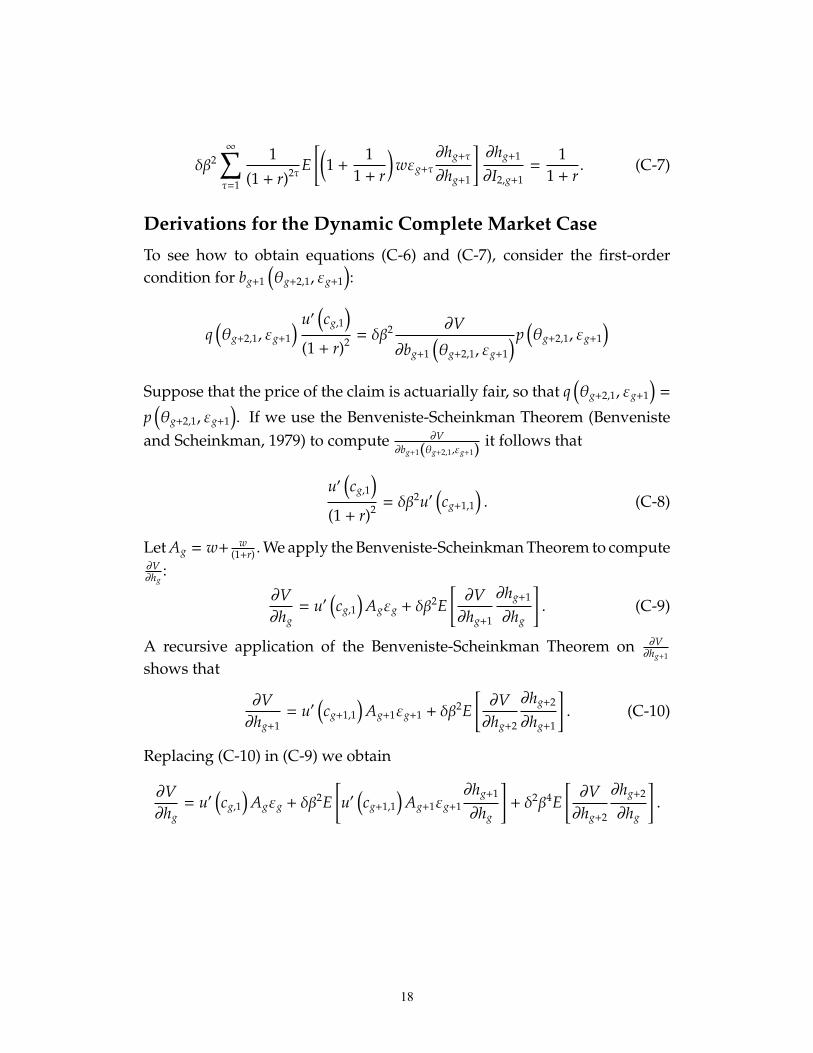
Derivations for the Dynamic Complete Market Case
To see how to obtain equations (C-6) and (C-7), consider the first-ordercondition for bg+1
(θg+2,1, εg+1
):
q(θg+2,1, εg+1
) u′(cg,1
)(1 + r)2 = δβ
2 ∂V
∂bg+1
(θg+2,1, εg+1
)p(θg+2,1, εg+1
)Suppose that the price of the claim is actuarially fair, so that q
(θg+2,1, εg+1
)=
p(θg+2,1, εg+1
). If we use the Benveniste-Scheinkman Theorem (Benveniste
and Scheinkman, 1979) to compute ∂V∂bg+1(θg+2,1,εg+1) it follows that
u′(cg,1
)(1 + r)2 = δβ
2u′(cg+1,1
). (C-8)
Let Ag = w+ w(1+r) .We apply the Benveniste-Scheinkman Theorem to compute
∂V∂hg
:
∂V∂hg= u′
(cg,1
)Agεg + δβ
2E[∂V∂hg+1
∂hg+1
∂hg
]. (C-9)
A recursive application of the Benveniste-Scheinkman Theorem on ∂V∂hg+1
shows that
∂V∂hg+1
= u′(cg+1,1
)Ag+1εg+1 + δβ
2E[∂V∂hg+2
∂hg+2
∂hg+1
]. (C-10)
Replacing (C-10) in (C-9) we obtain
∂V∂hg= u′
(cg,1
)Agεg + δβ
2E[u′
(cg+1,1
)Ag+1εg+1
∂hg+1
∂hg
]+ δ2β4E
[∂V∂hg+2
∂hg+2
∂hg
].
18

Continuining with the recursion we conclude that
∂V∂hg=
+∞∑τ=0
(δβ2
)τE[u′
(cg+τ,1
)Ag+τεg+τ
∂hg+τ
∂hg
].
Now, use (C-8) to obtain
∂V∂hg= u′
(cg,1
) +∞∑τ=0
1
(1 + r)2τE[Ag+τεg+τ
∂hg+τ
∂hg
]. (C-11)
By replacing (C-11) into (C-4) and (C-5) we obtain (C-6) and (C-7).
19

D Program Definitions, Tables and Figures
Descriptions of Intervention Programs Discussed in the Text
Head Start. Head Start is a national program targeted to low-income pre-school aged children (ages 3–5) that promotes school readiness byenhancing their social and cognitive development through the pro-vision of educational, health, nutritional, social and other services toenrolled children and families. There is a new program, Early HeadStart, that begins at age 1.
Perry Preschool Program. The Perry preschool experiment was an inten-sive family enhancement preschool program administered to ran-domly selected disadvantaged black children enrolled in the programover five different waves between 1962 and 1967. Children were en-rolled 2 1
2 hours per day, 5 days a week, during the school year andthere were weekly 1 1
2 -hour home visits. They were treated for 2 years,ages 3 and 4. A control group provides researchers with an appropriatebenchmark to evaluate the effects of the preschool program.
The Abecedarian Project. The Abecedarian Project recruited children bornbetween 1972 and 1977 whose families scored high on a “High Risk”index. It enrolls and enriches the family environments of disadvan-taged children beginning a few months after birth and continuing untilage 5. At age 5—just as they were about to enter kindergarten—allof the children were reassigned to either a school age interventionthrough age 8 or to a control group. The Abecedarian program wasmore intensive than the Perry program. Its preschool program was ayear-round, full-day intervention.
Chicago Parent-Child Center. The CPC was started in 1967, in selectedpublic schools serving impoverished neighborhoods of Chicago. Us-ing federal funds, the center provided half-day preschool program fordisadvantaged 3- and 4-year-olds during the 9 months that they werein school. In 1978, state funding became available, and the programwas extended through third grade and included full-day kindergarten.
20

Tables
D1 Economic benefits and costs
D2 Test Scores and the Timing of Income: White Males, CNLSY/1979
Figures
1 Repeated from published paper, Children of NLSY, Average Standard-ized Score, PIAT Math by Permanent Income Quartile
D0 Trend in Mean Cognitive Score by Maternal Education
D00 Children of NLSY: Average Standarized Score, Peabody Picture Vo-cabulary Test by Permanent Income Quartile
D1a Children of NLSY: Average percentile rank on PIAT Math score, byincome quartile
D1b Children of NLSY: Adjusted average PIAT Math score percentiles, byincome quartile
D2a Children of NLSY: Average percentile rank on anti-social behaviorscore, by income quartile
D2b Children of NLSY: Adjusted average anti-social behavior score per-centile, by income quartile
D3a Children of NLSY: Average percentile rank on anti-social behaviorscore, by race
D3b Children of NLSY: Adjusted average anti-social behavior score per-centile, by race
D4a Early Childhood Longitudinal Study (ECLS): (a) Reading
D4b Mean trajectories, high and low poverty schools (ECLS): (b) Math
D5a Average trajectories, grades 1–3, high and low poverty schools (Sus-taining Effects Study): (a) Reading
D5b Average trajectories, grades 1–3, high and low poverty schools (Sus-taining Effects Study): (b) Math
D6a Average achievement trajectories, grades 8–12 (NELS 88): (a) Science
21

D6b Average achievement trajectories, grades 8–12 (NELS 88): (b) Math
D7a Growth as a function of student social background (ECLS): (a) Reading
D7b Growth as a function of student social background (ECLS): (b) Math
D8a Growth as a function of school poverty for poor children (SustainingEffects Study): (a) Reading
D8b Growth as a function of school poverty for poor children (SustainingEffects Study): (b) Math
D9a Perry Preschool Program: IQ, by age and treatment group
D9b Perry Preschool Program: educational effects, by treatment group
D9c Perry Preschool Program: economic effects at age 27, by treatmentgroup
D9d Perry Preschool Program: arrests per person before age 40, by treat-ment group
D10a College participation of HS graduates and GED holders: white males
D10b College participation by race: dependent high school graduates andGED holders (males, 18–24)
22
Perry Chicago CPC
Child Care 986 1,916
Earnings 40,537 32,099
K-12 9,184 5,634
College/Adult -782 -644
Crime 94,065 15,329
Welfare 355 546
FG Earnings 6,181 4,894
Abuse/Neglect 0 344
Total Benefits 150,525 60,117
Total Costs 16,514 7,738
Net Present Value 134,011 52,380
Benefits-To-Costs Ratio 9.11 7.77
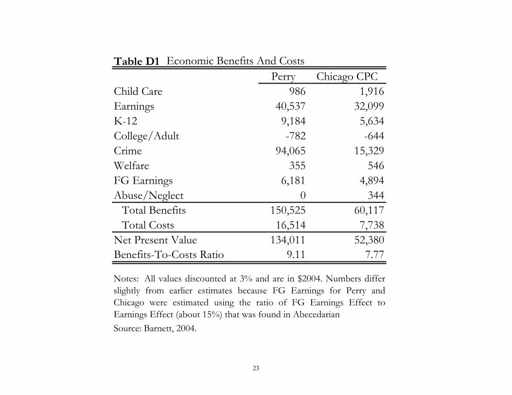
Table D1 Economic Benefits And Costs
Notes: All values discounted at 3% and are in $2004. Numbers differ
slightly from earlier estimates because FG Earnings for Perry and
Chicago were estimated using the ratio of FG Earnings Effect to
Earnings Effect (about 15%) that was found in Abecedarian
Source: Barnett, 2004.
23

Coefficient t-statistic Coefficient t-statistic Coefficient t-statistic Coefficient t-statisticFamily Permanent Income 0-14b 0.1899 4.1300 0.2963 3.5600 0.2877 2.8200 0.1879 2.2400Family Permanent Income 0-4c -0.1224 -1.5800Family Permanent Income 5-9d -0.0527 -0.6400Family Permanent Income 10-14e 0.0346 0.5900Mother's Abilityf 0.2729 9.5700 0.2742 9.4600 0.2607 8.9500 0.2606 8.8100Mother's Age at Test Date 0.0070 1.1500 0.0069 1.0700 0.0059 0.9400 0.0053 0.8400Constant -0.9315 -3.8600 -0.8847 -3.5100 -1.0599 -4.2400 -0.9916 -4.0000Number of ObservationsR2
cFamily Permanent Income from age 0 to age 4 of the child. It is the average (inflation-adjusted) family income from age 0 to age 4 of the child. dFamily Permanent Income from age 5 to age 9 of the child. It is the average (inflation-adjusted) family income from age 5 to age 9 of the child. eFamily Permanent Income from age 10 to age 14 of the child. It is the average (inflation-adjusted) family income from age 10 to age 14 of the child. fAFQT of the Mother (NLSY/79).
White Males, CNLSY/1979
Table D2
aThe Ability Factor at ages 12-13 is obtained in the following way. First, we standardize the scores in PIAT Math and PIAT Reading Recognition so that at each age each score has mean zero and variance one. Then, we factor analyze the scores at each age and extract one factor. The factor values at age 12 and age 13 are combined to form only one factor. Let f12, f13 denote the factors at age 12 and 13, respectively. Let d12 take the value one if the factor at age 12 is nonmissing. Let d13 take the value one if the factor at age 13 is nonmissing. Then we construct the factor f as f = d12*f12 + (1-d12)*d13*f13.bFamily Permanent Income from age 0 to age 14 of the child. It is the average (inflation-adjusted) family income from age 0 to age 14 of the child.
Test Scores and the Timing of Income
8710.1777
8600.1739
883
Ability Factor at ages 12-13a
Ability Factor at ages 12-13a
0.1748855
0.1718
Ability Factor at ages 12-13a
Ability Factor at ages 12-13a
24

Figure 1Children of the NLSY
Average Standardized ScorePIAT Math by Permanent Income Quartile
-0.8000
-0.6000
-0.4000
-0.2000
0.0000
0.2000
0.4000
0.6000
0.8000
5 6 7 8 9 10 11 12 13 14
Age
Bottom Quartile Second Quartile Third Quartile Top Quartile
This figure shows the average standardized score in the PIAT Math test from ages 5 to 14 by quartile of familypermanent income. The sample consists of all Children of NLSY/79. Family permanent income is the mean familyincome from age 0 to age 18 of the child. At each age, we standardize the PIAT math score so it has mean zero andvariance one. That is, let mi,t denote the score of child i at age t. Let µt, σ
2t denote the mean and variance of the
PIAT-Math score at age t. We construct the variable zi,t as:
zi,t =mi,t − µt
σt
We then proceed by calculating the mean zi,t by quartile of family income. Let 1 (qi = Qj) denote the function thattakes the value one if the family permanent income of child i is in quartile Qj and zero otherwise. Let z̄j,t denotethe mean standardized score at age t of the children whose permanent income is in quartile Qj :
z̄j,t =∑
i zi,t1 (qi = Qj)∑i 1 (qi = Qj)
25
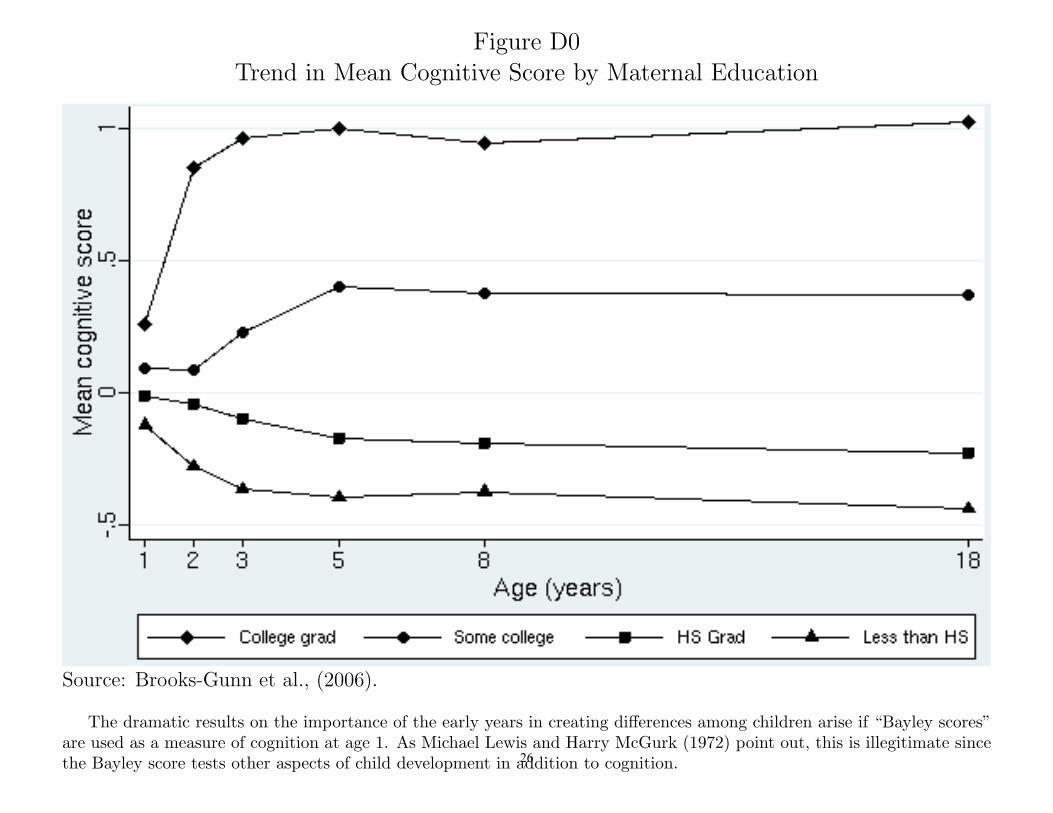
Figure D0Trend in Mean Cognitive Score by Maternal Education
Source: Brooks-Gunn et al., (2006).
The dramatic results on the importance of the early years in creating differences among children arise if “Bayley scores”are used as a measure of cognition at age 1. As Michael Lewis and Harry McGurk (1972) point out, this is illegitimate sincethe Bayley score tests other aspects of child development in addition to cognition.26

Figure D00Children of NLSY
Average Standardized Score Peabody Picture Vocabulary Test by Permanent Income Quartile
-0.8000
-0.6000
-0.4000
-0.2000
0.0000
0.2000
0.4000
0.6000
0.8000
3 4 5 6 7 8 9 10 11 12 13 14
Age
Bottom Quartile Second Quartile Third Quartile Top QuartileelitrauQ poT
Source: Full Sample of Children of the National Longitudinal Survey of Youth. Please see our website for a full explanation of this figure. 27

D1a
28

D1b
29

D2a
a s behavior s
30

D2b
behavior
31

D3abehavior
32

D3bbehavior
33

Early Childhood Longitudinal Study (ECLS)
(a) Reading
10
20
30
40
50
60
70
55 65 75 85
Age (months)
Rea
ding
Sco
re
Low povertyHigh povery
Figure D4a
Source: Raudenbush (2006)34

Mean trajectories, high and low poverty schools (ECLS)
(b) Math
10
20
30
40
50
60
55 65 75 85
Age (months)
Mat
h Sc
ore
Low povertyHigh poverty
Figure D4b
Source: Raudenbush (2006)35

Average trajectories, Grades 1-3, high and low poverty schools (Sustaining Effects Study)
(a) Reading
350
400
450
500
550
70 75 80 85 90 95
Age (months)
Rea
ding
Sco
re
Low povertyHigh Poverty
Figure D5a
Source: Raudenbush (2006)36

Average trajectories, Grades 1-3, high and low poverty schools (Sustaining Effects Study)
(b) Math
350
400
450
500
550
70 75 80 85 90 95
Age (months)
Mat
h Sc
ore
Low povertyHigh poverty
Figure D5b
Source: Raudenbush (2006)37

Average achievement trajectories, Grades 8-12 (NELS 88).(a) Science
15
20
25
30
8 10 12
Grade
Scie
nce
Scor
e
Low povertyHigh poverty
Figure D6a
Source: Raudenbush (2006)
38
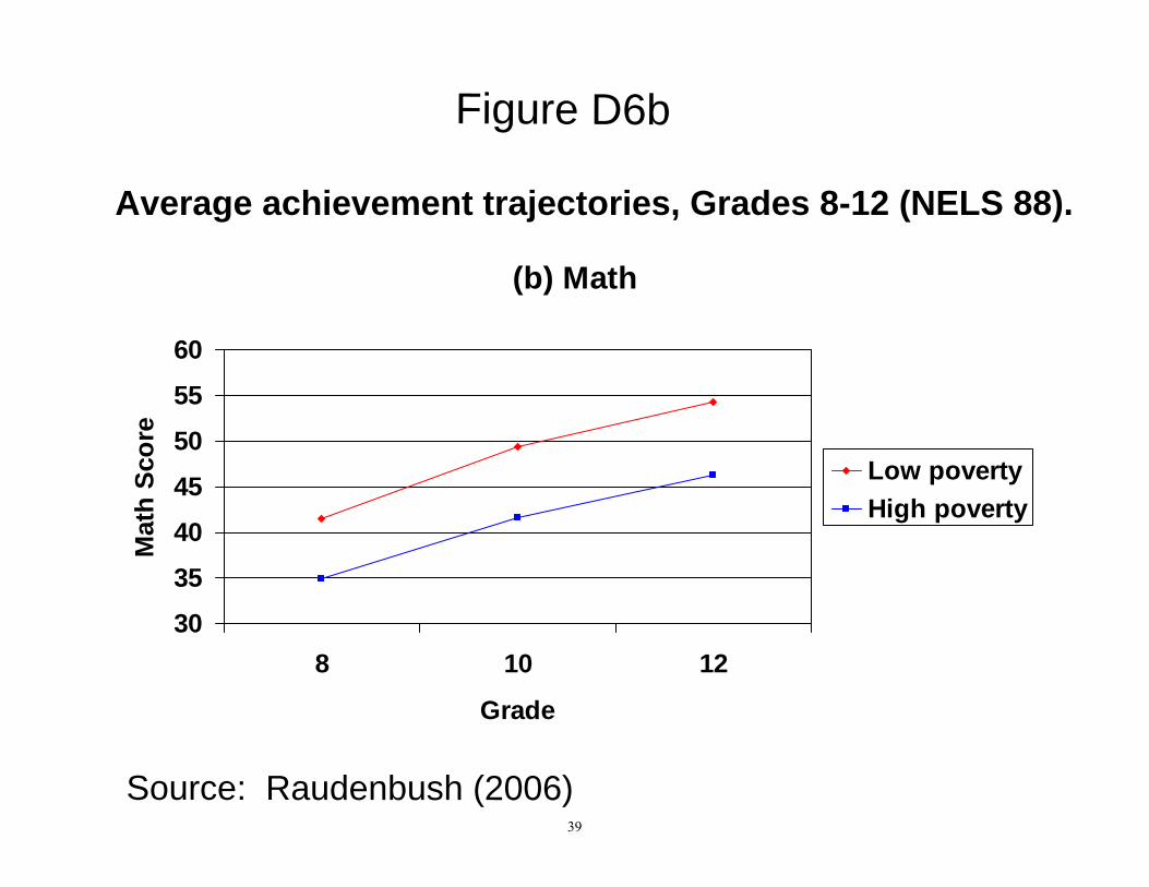
Average achievement trajectories, Grades 8-12 (NELS 88).
(b) Math
30
35
40
45
50
55
60
8 10 12
Grade
Mat
h Sc
ore
Low povertyHigh poverty
Figure D6b
Source: Raudenbush (2006)39

Growth as a function of student social background: ECLS
(a) Reading
10
20
30
40
50
60
70
55 65 75 85
Age (months)
Rea
ding
Sco
re
Hi SESLow SES
Figure D7a
Source: Raudenbush (2006)40

Growth as a function of student social background: ECLS
(b) Math
10
20
30
40
50
60
70
55 65 75 85
Age (months)
Mat
h Sc
ore
Hi SESLow SES
Figure D7b
Source: Raudenbush (2006)41
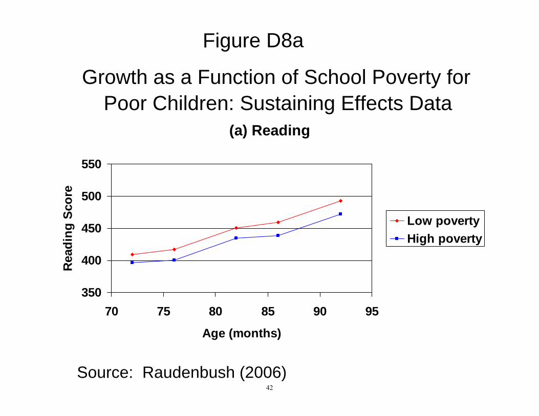
Growth as a Function of School Poverty for Poor Children: Sustaining Effects Data
(a) Reading
350
400
450
500
550
70 75 80 85 90 95
Age (months)
Rea
ding
Sco
re
Low povertyHigh poverty
Figure D8a
Source: Raudenbush (2006)42
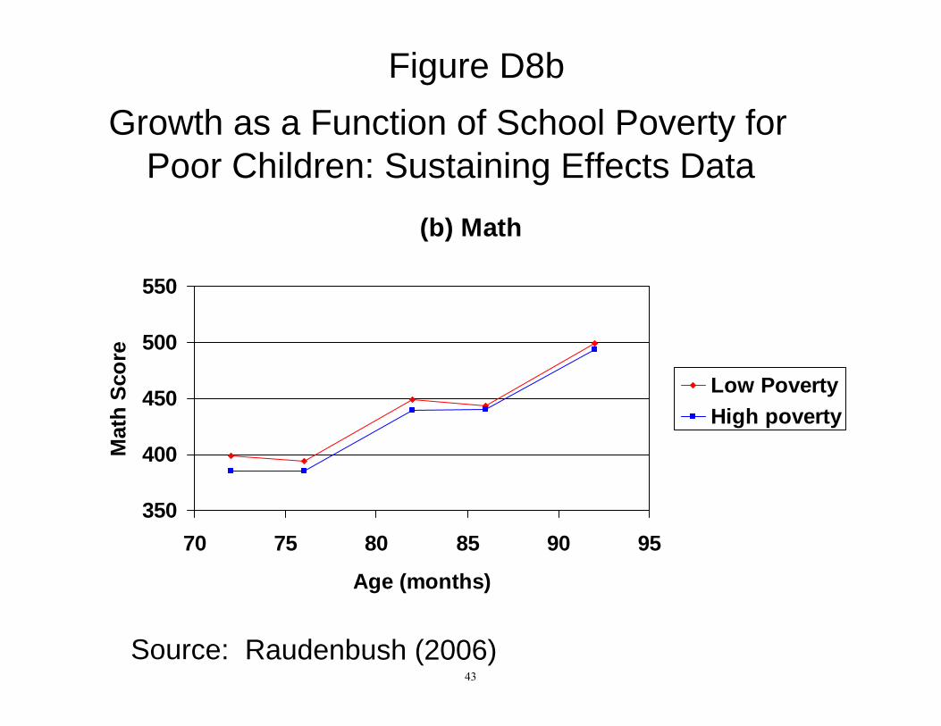
Growth as a Function of School Poverty for Poor Children: Sustaining Effects Data
(b) Math
350
400
450
500
550
70 75 80 85 90 95
Age (months)
Mat
h Sc
ore
Low PovertyHigh poverty
Figure D8b
Source: Raudenbush (2006)43

79.6
95.5 94.9
91.3 91.7
88.1 87.7
85
78.5
83.3 83.5
86.387.1 86.9 86.8
84.6
75
80
85
90
95
100
IQ
4 5 6 7 8 9 10Entry
Age
Treatment Group Control Group
Source: Perry Preschool Program. IQ measured on the Stanford Binet Intelligence Scale (Terman & Merrill, 1960).Test was administered at program entry and each of the ages indicated.
Perry Preschool Program: IQ, by Age and Treatment Group
Figure D9a
44

45%
66%
15%
49%
34%
15%
0% 10% 20% 30% 40% 50% 60% 70%
On Time Grad.from HS
High Achievementat Age 14*
SpecialEducation
Source: Barnett (2004).Notes: *High achievement defined as performance at or above the lowest 10th percentile on the California AchievementTest (1970).
Perry Preschool Program: Educational Effects, by Treatment Group
Figure D9b
Treatment Control
45

14%
29%
13%
36%
7%
29%
0% 10% 20% 30% 40%
Never on Welfareas Adult*
Own Home
Earn +$2,000Monthly
Source: Barnett (2004). *Updated through Age 40 using recent Perry Preschool Program data, derived from self reportand all available state records.
Perry Preschool Program: Economic Effects at Age 27, by Treatment Group
Figure D9c
Treatment Control
46

1.2 3.9 .4
2.1 6.7 .6
0 2 4 6 8 10
Treatment
Control
Source: Perry Preschool Program. Juvenile arrests are defined as arrests prior to age 19.
Perry Preschool Program: Arrests per Person before Age 40, by Treatment Group
Figure D9d
Felony Misdemeanor Juvenile
47

D10a: College participation of HS graduates and GED holdersWhite Males
40.00%
45.00%
50.00%
55.00%
60.00%
65.00%
70.00%
75.00%
80.00%
85.00%
90.00%
1970
1972
1974
1976
1978
1980
1982
1984
1986
1988
1990
1992
1995
1997
1999
Perc
enta
ge
Family income bottom quartile Family income third quartile Family income top half
White Females
30.00%
40.00%
50.00%
60.00%
70.00%
80.00%
90.00%
100.00%
1970
1972
1974
1976
1978
1980
1982
1984
1986
1988
1990
1992
1995
1997
1999
Perc
ent
High School Graduates of Regular Day School Programs, Public and PrivatePercentage of 17 Year Olds
USA, 1971-1999
66.0
68.0
70.0
72.0
74.0
76.0
78.0
1971
1972
1973
1974
1975
1976
1977
1978
1979
1980
1981
1982
1983
1984
1985
1986
1987
1988
1989
1990
1991
1992
1993
1994
1995
1996
1997
1998
1999
Source: (1) the Department of Education National Center for Education Statistics and (2) American Council on Education, General Educational Development Testing Service.
Family Income Bottom Quartile Family Income Third Quartile Family Income Top Half
48

D10b: College participation by race Dependent high school graduates and GED holders
Males, ages eighteen to twenty-four
0.4
0.45
0.5
0.55
0.6
0.65
0.7
1971
1973
1975
1977
1979
1981
1983
1985
1987
1989
1991
1993
1995
1997
Year
Rat
e
White Black HispanicNote: Three-year moving averages are shown
49

References
Becker, G. S. and N. Tomes (1986, July). Human capital and the rise and fallof families. Journal of Labor Economics 4(3, Part 2), S1–S39.
Ben-Porath, Y. (1967, August). The production of human capital and the lifecycle of earnings. Journal of Political Economy 75(4, Part 1), 352–365.
Benveniste, L. M. and J. A. Scheinkman (1979, May). On the differentiabilityof the value function in dynamic models of economics. Econometrica 47(3),727–732.
Brooks-Gunn, J., F. Cunha, G. Duncan, J. J. Heckman, and A. Sojourner(2006). A reanalysis of the IHDP program. Unpublished manuscript,Infant Health and Development Program, Northwestern University.
Carneiro, P., F. Cunha, and J. J. Heckman (2003, October 17). Interpretingthe evidence of family influence on child development. In The Economicsof Early Childhood Development: Lessons for Economic Policy, Minneapo-lis, Minnesota. The Federal Reserve Bank. Presented at ”The Economicsof Early Childhood Development: Lessons for Economic Policy Confer-ence,” Minneapolis Federal Reserve Bank, Minneapolis, MN. October 17,2003.
Cunha, F. and J. J. Heckman (2007a). Formulating, identifying and estimat-ing the technology of cognitive and noncognitive skill formation. Un-published manuscript, University of Chicago, Department of Economics.Forthcoming, Journal of Human Resources.
Cunha, F. and J. J. Heckman (2007b, May). The technology of skill formation.American Economic Review 97(2). Forthcoming.
Heckman, J. J. and Y. Rubinstein (2001, May). The importance of noncog-nitive skills: Lessons from the GED testing program. American EconomicReview 91(2), 145–149.
Heckman, J. J., J. Stixrud, and S. Urzua (2006, July). The effects of cognitiveand noncognitive abilities on labor market outcomes and social behavior.Journal of Labor Economics 24(3), 411–482.
Keating, D. P. and C. Hertzman (Eds.) (1999). Developmental Health and theWealth of Nations: Social, Biological, and Educational Dynamics. New York:Guilford Press.
50