websem aero acoustic simulation dec2013
TRANSCRIPT

Restricted © LMS International 2013 All rights reserved.
Flow-induced noise simulationVirtual.Lab Acoustics Rev12Raphael Hallez – Product Manager Acoustics

20XX-XX-XX
Restricted © LMS International 2013 All rights reserved.
Page 2
Flow phenomena
What happens in the presence of flow ?
Wave convection:
- Significant at high Mach (M=vflow/c>0.3)
- Flow is NOT the noise source
- Flow influences the wave propagation
- Example: Aeroengine Inlet, muffler,…
Steady
Flow
Noise Source
Wave propagation is modified by flow
Flow-induced vibrations:
- Fluctuations from unsteady turbulent flow
- Flow acts as a loading of the flexible structure
- Example: Aircraft fuselage TBL loading, train
door,…
Turbulent
Flow
Structural vibrations
Structure-borne noise
Flow-induced noise � Aeroacoustics:
- Fluctuations from unsteady turbulent flow
- Flow acts as a noise source
- Acoustic waves propagate in medium at rest or are
convected by the mean flow component
- Example: pantograph, landing gear, cooling fan,…
Turbulent
Flow
Flow fluctuations
Flow-induced noise

20XX-XX-XX
Restricted © LMS International 2013 All rights reserved.
Page 3
Flow-Induced Noise phenomena
• Flow-induced noise = noise generated by turbulent flow
phenomena
• Vortices, turbulent eddies
• Vortex shedding (von Karman vortex street)
• Turbulent boundary layers and boundary layer separation
• Rotating surfaces in a fluid (propellers, fans)
• Level of turbulence in the flow, characterized by Reynolds number:
• Low Re � Large flow scales
• High Re � Large flow scales + smaller flow scales
• Unsteady vortices on many scales interact with each other and with
steady or moving surfaces ���� Noise generation
µ
ρVL=Re
SpeedSound
VelocityFlowMach =

20XX-XX-XX
Restricted © LMS International 2013 All rights reserved.
Page 4
Flow-induced noise simulation examples
• External Aeroacoustics:
• Turbulent flow interacts with static body and radiates noise outside
• Challenge: Capture the sources and reflection/scattering on large
surfaces
• Train bogie, Landing Gear, Wiper
• Internal Aeroacoustics / Confined flow:
• Propagation of sources (duct noise and blower noise) in ducting
system and radiation through outlet
• Challenge: Capture the acoustic reflections on duct walls (guided
waves)
• HVAC, exhaust, intake, ECS
• Mixed Internal-External Aeroacoustics
• Transmission through flexible panel � Aero-Vibro-Acoustics
• Challenge: Capture Hydrodynamic+Acoustic loading, capture
dynamics of system
• Windnoise (side mirror, A-pillar), fuselage TBL

20XX-XX-XX
Restricted © LMS International 2013 All rights reserved.
Page 5
Flow-Induced Noise : A Challenge for Numerical Simulation
� Acoustic field = part of the flow field � most straightforward approach: Direct Computational AeroAcoustics (CAA) (=direct numerical simulation of both the unsteady turbulent flow and the noise it generates)
But not practical because :
� High order schemes needed to capture acoustic propagation (numerical instabilities)
� High numerical cost of a direct CAA � prohibitive at low Mach and high Reynolds numbers
� Also, specific issues related to CFD discretisation techniques applied to acoustics
• Dissipation and dispersion errors
• Non-reflecting Boundary conditions
p’ = 4.4934739 Pa
hydrodynamicfield
acousticfield
� at low - moderate Mach numbers: orders of magnitude of difference between
• Length scales: λac = Lturb / M
• Magnitudes: O(M4) of the flow energy radiates into the far field
20XX-XX-XX
Restricted © LMS International 2013 All rights reserved.
Page 6
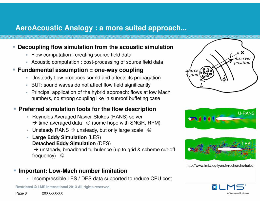
AeroAcoustic Analogy : a more suited approach...
� Decoupling flow simulation from the acoustic simulation
� Flow computation : creating source field data
� Acoustic computation : post-processing of source field data
� Fundamental assumption = one-way coupling
� Unsteady flow produces sound and affects its propagation
� BUT: sound waves do not affect flow field significantly
� Principal application of the hybrid approach: flows at low Mach
numbers, no strong coupling like in sunroof buffeting case
sourceregion
observerposition
L
λ
d
� Preferred simulation tools for the flow description
� Reynolds Averaged Navier-Stokes (RANS) solver
� time-averaged data � (some hope with SNGR, RPM)
� Unsteady RANS � unsteady, but only large scale �
� Large Eddy Simulation (LES)
Detached Eddy Simulation (DES)
� unsteady, broadband turbulence (up to grid & scheme cut-off
frequency) ☺
� Important: Low-Mach number limitation
� Incompressible LES / DES data supported to reduce CPU cost
http://www.lmfa.ec-lyon.fr/recherche/turbo
U-RANS
LES

20XX-XX-XX
Restricted © LMS International 2013 All rights reserved.
Page 7
Aero-Acoustic Sources
Turbulent Flow
Moving Surfaces
Steady Surfaces
No Surfaces
(or smooth surfaces)
Quadrupoles
Dipoles on surfaces (+ Quadrupoles in wake)
Rotating Dipoles (+ Quadrupoles in wake)

20XX-XX-XX
Restricted © LMS International 2013 All rights reserved.
Page 8
Source Generation in Virtual.Lab
Dipole Sources
• Flow-induced noise in presence of static surfaces with compact regions
• Requires pressure data on the walls (compressible or incompressible)
Quadrupole Sources :
• Flow-induced noise without presence of surfaces (turbulent jets) or non-
compact regions
• Requires velocity vector data in flow volume
Fan Sources = Rotating Dipoles Sources
• Flow-induced noise caused by rotating surfaces (fan)
• Requires pressure data on one or all blades surface for multiple
revolutions

20XX-XX-XX
Restricted © LMS International 2013 All rights reserved.
Page 9
Simulation Process based on Aeroacoustic analogy
Fluid Dynamics
AcousticsTransient CFD
Simulation
Aeroacoustic sources
Virtual.Lab Acoustics Computation
Data Mapping + Fourier Transform
Acoustics Results
Turbulent Flow Field

20XX-XX-XX
Restricted © LMS International 2013 All rights reserved.
Page 10
CFD-Acoustics Coupling in Virtual.Lab
VIRTUAL.LAB supports CFD data stored in CGNS
format files (CFD General Notation System)
Following commercial CFD codes already support
CGNS export for aero-acoustical data :
• CFX (Ansys)
• FLUENT (Ansys)
• STAR-CD 4 / STAR-CCM+ (CD Adapco)
• PowerFlow (EXA)
• CFD++ (Metacomp)
• SCRYU/Tetra (Cradle Software)
• Fine Turbo (Numeca)
• OpenFoam

20XX-XX-XX
Restricted © LMS International 2013 All rights reserved.
Page 11
What can Virtual.Lab do more than CFD alone?
Effect of acoustics on flow (strong feedback)
far-field scattering
Absorbing materials
Flow-induced vibration
CFD Direct CAA � � � �CFD postprocessing(FWH) � � � �Hybrid Approach
(CFD + Virtual.Lab) � � � �

20XX-XX-XX
Restricted © LMS International 2013 All rights reserved.
Page 12
Dipole sources from Compressible CFD ���� Curle
• Curle’s solution (1955) to Lighthill’s equation in presence of solid rigid boundaries (neglecting viscous effects)
• Quadrupole incident field negligible for low Mach numbers (Power ratio = M2)
• Mathematically exact solution But: Pf must satisfy acoustic boundary conditions
• OK if the flow description is compressible
• if the flow description is incompressible and surface is not acoustically compact, the solution is inaccurate (missing acoustic reflection and scattering effects)
Quadrupoles (negligible
at low Mach numbers)Dipole Surface pressure

20XX-XX-XX
Restricted © LMS International 2013 All rights reserved.
Page 13
Curle’s analogy: what the compactness assumption means
� Curle assumes the CFD captures all acoustic effects on the source surfaces (hydrodynamic pressure+acoustic scattered pressure)
� Not true for incompressible CFD or non-compact surfaces
� Surface with sources will be seen as acoustically transparent!

20XX-XX-XX
Restricted © LMS International 2013 All rights reserved.
Page 14
Dipole sources from Incompressible CFD ����Neumann Dipoles
Import CFD pressure Pf and define surface
dipoles
Transform dipoles into
acoustic (Neumann) BCs
Compute acoustic solution
• flow wall pressure can be used to define appropriate boundary conditions of an equivalent acoustic boundary value problem
• If flow is compressible � equivalent to Curle
• If flow is incompressible, G is the Green’s function of Laplace problem (infinite sound speed)
� More flexible: can be applied to Indirect BEM and FEM
� More accurate than standard Curle (recomputes acoustic scattering and reflection effects)

20XX-XX-XX
Restricted © LMS International 2013 All rights reserved.
Page 15
Example: Trailing edge noise prediction based on incompressible-flow pressure
Reference solution
Curle
New formulation

20XX-XX-XX
Restricted © LMS International 2013 All rights reserved.
Page 16
Virtual.Lab AeroAcoustics - Slide 16
Flow:
Acoustic:
Example: Rod-Airfoil Noise prediction based on incompressible-flow pressure
FEM mesh

20XX-XX-XX
Restricted © LMS International 2013 All rights reserved.
Page 1717 copyright LMS International - 2010
Example: Rod-Airfoil Noise prediction based on incompressible-flow pressure
•Comparison with measurements
Neumann dipoles
1 freq 495 freq 4 cores
FEM Neumann Incompressible 2min+10s 11min+1h20 3min+20 min

20XX-XX-XX
Restricted © LMS International 2013 All rights reserved.
Page 18
Virtual.Lab Aero-Acoustics
Dipole Source Generation – Step by step
Import CFD surface pressure data
(centroids/nodes)
Map CFD pressure on acoustic mesh + Fourier transform

20XX-XX-XX
Restricted © LMS International 2013 All rights reserved.
Page 19
Virtual.Lab Aero-Acoustics
Dipole Source Generation – Step by step
Define Surface Dipole Boundary Condition (distributed dipoles are defined on
acoustic mesh � boundary condition)
Solve the acoustic response case (FEM or BEM) + post-process…

20XX-XX-XX
Restricted © LMS International 2013 All rights reserved.
Page 20
Virtual.Lab Aero-Acoustics
Special feature : Conservative mapping
���� Specific conservative mapping algorithm to preserve information
over a large range of flow scales:
Fine CFD mesh Coarse Acoustic mesh
Map turbulent flow field
� Flow scales very small
� CFD mesh has extremely
small cells (Millions of DOFs)
� Acoustic wavelength large
compared to Flow scales
� Acoustic mesh coarser than
CFD mesh (Lelement=~λ/6)
∫∫ =
MeshAcousticMeshCFD
PdSpds

20XX-XX-XX
Restricted © LMS International 2013 All rights reserved.
Page 21
Quadrupole sources for more complex problems
(for high Reynolds number, isentropic flow and low Mach
number)
• Lighthill’s equation : incident field from quadrupoles + scattering on surfaces
• more generic :
• non compact source regions
• Aero-vibro-acoustics
• Higher flow speed
• But:
• Difficult to deal with volume data set
• Singularity for sources close to walls
• Mapping from CFD to coarse acoustic mesh

20XX-XX-XX
Restricted © LMS International 2013 All rights reserved.
Page 22
Quadrupole sourcesNew formulation in Virtual.Lab R13
New implementation in Virtual.Lab R13:
• Best performance: supported by FEMAO solver (Adaptive order FEM)
• Improved Usability: CFD data directly read by solver (linux support)
• Improved Accuracy: No mapping required on intermediate mesh, no singularity issue.
� FEMAO = FEM Adaptive Order solver:
� Start from coarse mesh (less than 1 element /
wavelength!)
� Solver automatically increases the element order
at high frequency
� Most efficient FEM solver for broad frequency
computation
� Most accurate scattering modeling
� Up to 20 times Less memory and faster
computation time than standard FEM!
FEMAO Acoustic mesh
36 000 nodes
Max freq FEM: 200 Hz
Max freq FEMAO: 4000 Hz

20XX-XX-XX
Restricted © LMS International 2013 All rights reserved.
Page 23
Fan noise components
• Aeronautical
• Energy
• Automotive
Fan Noise
Tonal (Discrete Frequency)
Broadband
Unsteady pressure fluctuations on the blade surface
Incoming turbulence (Leading edge)
Self-noise (Trailing edge)
Tip vortex shedding
Component Source

20XX-XX-XX
Restricted © LMS International 2013 All rights reserved.
Page 24
Rotor-stator configuration – noise generation mechanisms
1 Rotor leading-edge noise 2 Rotor trailing-edge noise 3 Wake interaction noise on stator
� Interaction of inflow turbulence with leading edge
� Depends on inflow turbulence
� Modeled with fan source
� Interaction of boundary layer with trailing edge
� Important for high rotation speed
� Modeled with fan source
Flow
RROOTTOORR SSTTAATTOORR
� Interaction of rotor wake with stator
� Modeled with surface dipoles

20XX-XX-XX
Restricted © LMS International 2013 All rights reserved.
Page 25
FWH formulation for fan noise
Constructive interference:
sound of the total fan =
B x (sound of a single blade)
Sound
emitted at
BPFHs
Sum over
BLHs
Bessel function: modulation of
the Doppler frequency shift
during blade revolution
Radius where
force is applied Thrust
harmonic
Drag
harmonic
� Tonal fan noise formulation:
• Fan blade represented by a rotating point dipole (force obtained by
integration of CFD surface pressure)
• Rotation effects (Doppler shift) accounted for analytically (no rotating
mesh)
• If blade is large, automatically split into compact segments
• Captures both Tonal and Broadband components
• Needs unsteady pressure for multiple blade revolutions

20XX-XX-XX
Restricted © LMS International 2013 All rights reserved.
Page 26
Industrial Case Study
Radial Fan Noise : internal pressure distribution
Internal SPL distribution in the blower
ducts (around 3 kHz)� Observe intake and outlet
noise maxima in external SPL distribution
0
10
20
30
40
50
60
70
1 2 3 4 5 6 7 8 9
Microphones
Pre
ssu
re L
evel
dB
(A)
Measurement
Computed
20XX-XX-XX
Restricted © LMS International 2013 All rights reserved.
Page 27
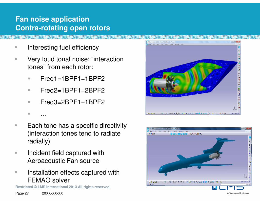
Fan noise applicationContra-rotating open rotors
� Interesting fuel efficiency
� Very loud tonal noise: “interaction
tones” from each rotor:
� Freq1=1BPF1+1BPF2
� Freq2=1BPF1+2BPF2
� Freq3=2BPF1+1BPF2
� …
� Each tone has a specific directivity
(interaction tones tend to radiate
radially)
� Incident field captured with
Aeroacoustic Fan source
� Installation effects captured with
FEMAO solver

20XX-XX-XX
Restricted © LMS International 2013 All rights reserved.
Page 28
Aero-acousticsExample HVAC Duct
Source regions
(vorticity)
Flow:
Acoustic:
Dipoles on the flap Far-field acoustic radiation
101
102
103
30
40
50
60
70
80
90
100
110
frequency (Hz)
SP
L (
dB
)
CFDexperiments (Jaeger et al. 2008)
Instantaneous velocity
From consortium of German car manufacturers - Audi, BMW, Daimler, Porsche and
Volkswagen where LMS participated

20XX-XX-XX
Restricted © LMS International 2013 All rights reserved.
Page 2910
110
210
330
40
50
60
70
80
90
100
110
frequency (Hz)
SP
L (
dB
)
CFDexperiments (Jaeger et al. 2008)
CFD results: pressure on the wall
C
101
102
103
30
40
50
60
70
80
90
100
110
frequency (Hz)
SP
L (
dB
)
CFDexperiments (Jaeger et al. 2008)
101
102
103
30
40
50
60
70
80
90
100
110
frequency (Hz)
SP
L (
dB
)CFDexperiments (Jaeger et al. 2008)
B
A
B
C
- Very good agreement downstream the flap
- Overprediction in the elbow separation region
A

20XX-XX-XX
Restricted © LMS International 2013 All rights reserved.
Page 30
Acoustic modeling
Source region (dipoles)
exterior field points
Inlet (absorbent panel Z = ρc)
� Aeroacoustic sources: distributed dipoles defined from CFD pressure
� Implementation in FEM: transformation of CFD pressure into equivalent
Neumann BCs (more details in AIAA2012-2070)
� 267 030 TETRA4 elements
� computation time: 10 s/freq
PML
FEM model

20XX-XX-XX
Restricted © LMS International 2013 All rights reserved.
Page 31
HVAC Flap Application case - accuracy
Acoustic radiation – Averaged over all measurement points:
New Neumann-based source modeling
Experimental
Numerical (FEM)

20XX-XX-XX
Restricted © LMS International 2013 All rights reserved.
Page 32
Virtual.Lab AeroAcoustics - Slide 32
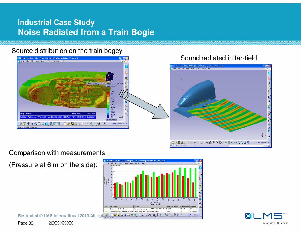
Industrial Case Study
Noise Radiated from a Train Bogie
High speed train - CFD done with EXA Powerflow (Lattice-Boltzman) – Courtesy of Bombardier
Surface Velocity magnitude Vorticity
Pressure coefficientVelocity magnitude
20XX-XX-XX
Restricted © LMS International 2013 All rights reserved.
Page 33
Virtual.Lab AeroAcoustics - Slide 33
Industrial Case Study
Noise Radiated from a Train Bogie
Comparison with measurements
(Pressure at 6 m on the side):
Source distribution on the train bogeySound radiated in far-field

20XX-XX-XX
Restricted © LMS International 2013 All rights reserved.
Page 34
Flow-induced Vibrations
� Flow acts as a structural pressure loading:
� pump vibration
� Windnoise (turbulence around A-pilar, mirror)
� turbulent Boundary layer loading on fuselage or hull
� How to get pressure loading?
� Directly from CFD (compressible)
� From Aeroacoustic source propagation (side mirror
noise)
� From analytical models (Corcos, Chase)
� How to compute vibro-acoustic response
� Apply loading on structural model (modal or direct)
� Compute vibration in a weakly or strongly-coupled
model
� Apply vibration as Boundary Condition for acoustic
model with FEMAO

20XX-XX-XX
Restricted © LMS International 2013 All rights reserved.
Page 35
Windnoise application case Description and modeling process
A-pillar Turbulence
Mic.
Glass Interior Walls
Outer Walls (Rigid)
External CFD
Model – Transient
Flow
Vibrating Surfaces
(Side Glass, Windshield)
Acoustics Model
(Car Interior)
Coupled Vibration & Acoustics Model
LMS Virtual.Lab Acoustics
Inflow
CFD Model
ANSYS Fluent
• Noise prediction at interior of the HSM (Hyundai Simplified Model released by
HKMC) caused by transient external aerodynamic sources around A-pillar

20XX-XX-XX
Restricted © LMS International 2013 All rights reserved.
Page 36
CFD Model
• CFD Domain consists of 45 million cells
• 2nd order implicit transient formulation (time step: 2.0e-
5s)
• Total physical time = 1 s (5120 time steps)
• 4 different cases: 110 and 130 km/h, 0 and 10 deg.
Yaw
• Solver : ANSYS Fluent (Pressure Based, Double
Precision, Transient , Gradient – Least Square Cell
Based)
• Turbulence Model Transient : DDES – SST K-Omega
• Total computation time: 15 days for the transient run
and 12 Hours for steady run with Intel 2*6 core Xeon
5680, 4 m/c connected via infiniband (total 48 cores)

20XX-XX-XX
Restricted © LMS International 2013 All rights reserved.
Page 37
Transient Flow Field of 110kph, 10deg Yaw
Velocity Contours at Z = 0.5 m Pressure Contours at Z = 0.5 m
Iso-surface of Q-Criterion colored by velocity magnitude

20XX-XX-XX
Restricted © LMS International 2013 All rights reserved.
Page 38
Flow
Vibration
Acoustics
Aero-Vibro-acoustic modeling strategy
� compressible flow simulation captures Unsteady Turbulent flow
� contains both hydrodynamic and acoustic components �
Directly applied as structural pressure loading
� Assume vibration has no influence on the flow � uncoupled flow-
vibration approach
� Structural FE model captures dynamics of structure
� Modal approach is used (with uniform modal damping)
� Windows vibration defined as Boundary condition for Acoustic
model.
� Assume Vibration is independent from fluid loading � weakly
coupled vibro-acoustic approach (OK for target frequencies)
� Acoustic radiation computed with FEM-AO solver (adaptive
order)

20XX-XX-XX
Restricted © LMS International 2013 All rights reserved.
Page 39
Structural model CFD loading
� CFD Surface Pressure is mapped onto Structural mesh in LMS Virtual.Lab
� 5120 time steps, dt = 2e-5s, T = 0.1s
� Pressure is transformed from time to frequency (df=10Hz) and applied as distributed
pressure loading
� No time averaging is performed here (could be done if time history is long enough to
improve convergence of predictions)
� Structural modes computed with LMS Virtual.Lab structural solver
CFD Pressure 500 Hz Structural mode shape Window FRF
20XX-XX-XX
Restricted © LMS International 2013 All rights reserved.
Page 40
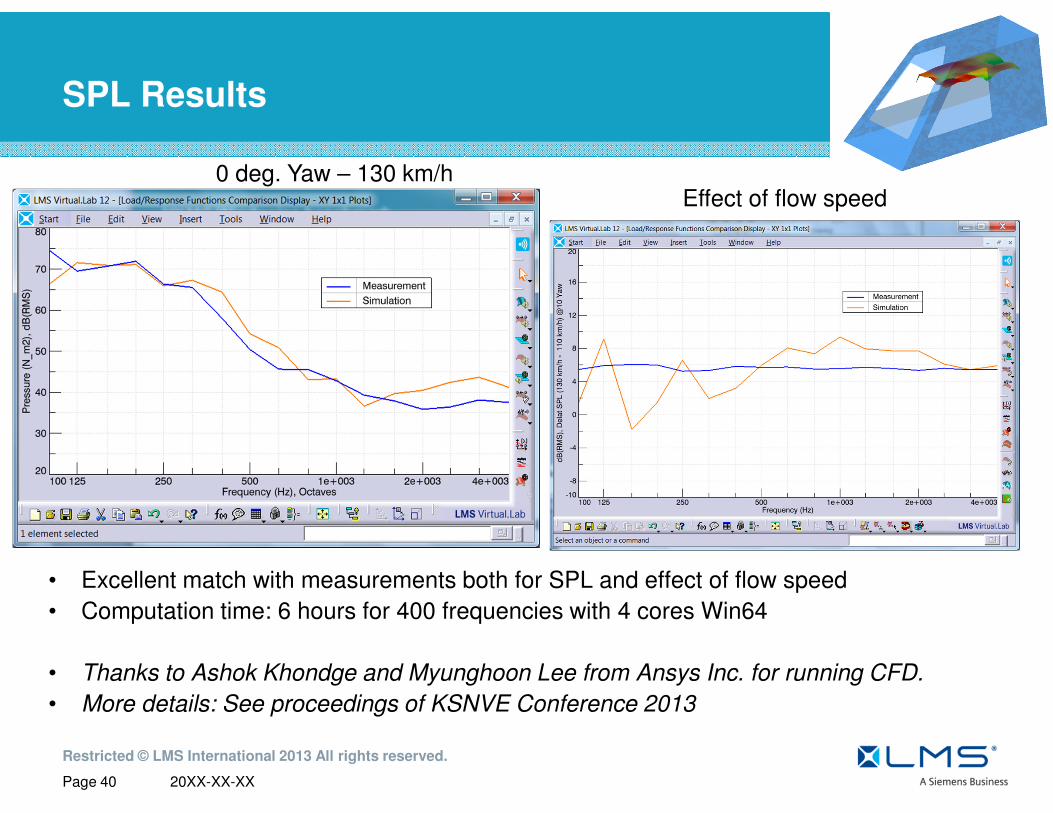
SPL Results
• Excellent match with measurements both for SPL and effect of flow speed
• Computation time: 6 hours for 400 frequencies with 4 cores Win64
• Thanks to Ashok Khondge and Myunghoon Lee from Ansys Inc. for running CFD.
• More details: See proceedings of KSNVE Conference 2013
0 deg. Yaw – 130 km/hEffect of flow speed

20XX-XX-XX
Restricted © LMS International 2013 All rights reserved.
Page 41
Conclusions
� Virtual.Lab Acoustics powerful tool for aero-acoustics simulation
� Various aeroacoustic sources for accurate modeling:
� Dipole sources for compressible and incompressible flow description
� Quadrupole sources in FEMAO solver
� Fan sources for tonal and broadband noise
� Virtual.Lab for Flow-induced vibrations:
� Integrated vibro-acoustic solver
� Poro-elastic and visco-elastic material modeling

20XX-XX-XX
Restricted © LMS International 2013 All rights reserved.
Page 42
Pour toutes informations complémentaires
Pour toutes informations complémentaires, vous pouvez contacter :
� Yohann MESMIN :
�T : +33 (0) 1 34 52 17 55
�M : +33 (0) 6 18 55 17 60