weighted nuclear norm minimization method for … ft.pdfweighted nuclear norm minimization method...
TRANSCRIPT
Weighted Nuclear Norm Minimization
Method for Massive MIMO Low-Rank
Channel Estimation Problem
A thesis submitted
in partial fulfillment for the degree of
Doctor of Philosophy
by
M.VANIDEVI
Department of Avionics
INDIAN INSTITUTE OF SPACE SCIENCE AND
TECHNOLOGYThiruvananthapuram - 695547
March 2018
CERTIFICATE
This is to certify that the thesis titled Weighted Nuclear Norm Minimization
Method for Massive MIMO Low-Rank Channel Estimation Problem,
submitted by M. Vanidevi, to the Indian Institute of Space Science and Technol-
ogy, Thiruvananthapuram, for the award of the degree of Doctor of Philosophy,
is a bonafide record of the research work done by her under our supervision. The
contents of this thesis, in full or in parts, have not been submitted to any other
Institute or University for the award of any degree or diploma.
Name of the Supervisor
Dr. N. Selvaganesan
Associate Professor
Department of Avionics, IIST
Place: Thiruvananthapuram
March 2018
i
DECLARATION
I declare that this thesis titled Weighted Nuclear Norm Minimization Method
for Massive MIMO Low-Rank Channel Estimation Problem submitted
in partial fulfillment of the Degree of Doctor of Philosophy is a record of orig-
inal work carried out by me under the supervision of Dr. N. Selvaganesan,
and has not formed the basis for the award of any degree, diploma, associateship,
fellowship or other titles in this or any other Institution or University of higher
learning. In keeping with the ethical practice in reporting scientific information,
due acknowledgments have been made wherever the findings of others have been
cited.
M. Vanidevi
SC10D014
Place: Thiruvananthapuram
March 2018
ii

ACKNOWLEDGEMENTS
I express my sincere gratitude to my guide Dr. N. Selvaganesan for guiding me
in my research study, for his patience and motivation. His guidance helped me in
all the time of research and useful suggestion in writing of this thesis. I could not
have imagined having a better advisor and mentor for my Ph.D. study.
Besides my guide, I would like to thank DC committee members Prof. Giridhar
IIT Madras, Dr. Apren VSSC, Dr.R. Lakshminarayan Avionics IIST, and Prof. K.
S. Subramanian Moosath IIST for their encouragement and insightful comments
during DC meeting.
My friends have rendered a good support to me in every aspect. Special thanks
to my IIST friends Dr.Chris Prema, Dr.Gigy. J. Alex, Prof. Nirmala R. James,
Prof. Honey John, Dr.Seena and Dr. Sheeba Rani, for their love and support.
I am thankful to Dr.Priyadarshan for helpful advice in writing my research
paper. I am also grateful to my colleagues in Avionics department for their support
throughout my research work.
Finally, I take this opportunity to express my deepest gratitude and love to
my family. Thanks to my husband and my daughters for all the patience and
understanding. Without them, this would not have been possible. I am also
thankful to my sisters, brother and my father-in-law for their unconditional love
and support all through my life. My dear father and mother have always been a
great support to me, helping me in all the ways possible. To them, I owe all that
I am and all that I have ever accomplished and it is to them that I dedicate this
thesis.
iii

ABSTRACT
In a cellular network, the demand for high throughput and reliable transmission
is increasing in large scale. One of the architectures proposed for 5G wireless
communication to satisfy the demand is Massive MIMO system. The massive
system is equipped with the large array of antennas at the Base Station (BS)
serving multiple single antenna users simultaneously i.e., number of BS antennas
are typically more compared to the number of users in a cell. This additional
number of antennas at the base station increases the spatial degree of freedom
which helps to increase throughput, maximize the beamforming gain, simplify the
signal processing technique and reduces the need of more transmit power. The
advantages of massive MIMO can be achieved only if Channel State Information
(CSI) is known at BS uplink and downlink operate on orthogonal channels - TDD
and FDD modes. We studied channel estimation for both modes.
In TDD system, the signals are transmitted in the same frequency band for
both uplink and downlink channel but in different time slots. Hence, uplink and
downlink channels are reciprocal. The estimation of the uplink channel is pre-
ferred, as the number of pilots used to estimate the channel is less compared to
the downlink channel. Most published research works have considered the rich
scattering propagation environment in uplink TDD mode (i.e., number of scatter-
ers tend to be infinity or more than the number of BS antenna and users in the
cell). Under rich scattering condition, the channel vector seen by any two users
are orthogonal. However, in realistic condition, the number of scatterers is finite.
In this thesis, the finite scattering propagation environment is considered for the
uplink TDD mode channel estimation problem. In finite scattering scenario, it is
assumed that the number of scatterers is less than the number of BS antenna and
users. Also, the scatterers are fixed and all users are facing the same scatterers.
When same scatterers are shared by all users, the correlation among the channel
vectors increases and correspondingly increases the spread of Eigen values of the
channel matrix. Hence, the high dimensional massive MIMO system is likely to
iv
have a low-rank channel.
The most conventional way of estimating the channel is by sending the pilot
or training sequences during the training phase in uplink. The Least Square
(LS) method estimates the channel based on the received signal and transmitted
training sequences by minimizing the mean square error. The main drawback of LS
estimation is that it does not impose the low-rank feature to the estimated channel
matrix. Therefore, to estimate the channel at the receiver, the channel estimation
problem can be formulated as a linearly constrained rank minimization problem.
Since, the nonconvex rank estimation is an NP hard problem, relaxed version of the
nonconvex rank minimization problem is formulated as the convex Nuclear Norm
Minimization (NNM) problem and solved using Majorization and Minimization
(MM) technique. In MM technique, the channel matrix is estimated iteratively by
successive minimization of the majorizing surrogate function obtained for the given
cost function. This successive minimization of the majorizer ensures that the cost
function decreases monotonically and guarantees global convergence of the convex
cost function. The iterative algorithm used to compute the channel estimates is
called Iterative Singular Value Thresholding (ISVT). In ISVT, all singular values
are equally penalized. However, the major information of the channel matrix is
associated with the larger singular values should be shrunk less compared to the
lower singular values. Therefore, nuclear norm minimization method leads to the
biased estimator. In ISVT, estimated singular value ignores the prior knowledge
of the singular values of the matrix. By utilizing the knowledge of singular value,
different shrunk can be applied to different singular values which lead to unbiased
estimation.
In this thesis, Weighted Nuclear Norm Minimization (WNNM) method which
includes the prior knowledge of singular value is proposed for channel estimation
problem. The WNNM is not convex in general case. By choosing the weights in
an ascending order, the nonconvex problem can be approximated to the convex
optimization problem which can be solved using MM technique. The solution to
the problem can be computed using Iterative Weighted Singular Value Threshold-
ing algorithm (IWSVT). To recover low-rank channel, the training matrix should
satisfy Restricted Isometric Property (RIP). The proposed algorithm is studied for
two different training sequences which satisfy the restricted isometric condition.
v

One of the orthogonal training sequence used is Partial Random Fourier Trans-
form matrix (PRFTM) which provides the iterative algorithm to converge in one
iteration. In order to obtain unbiased estimator, weights are chosen by minimizing
the Stein’s Unbiased Risk Estimator (SURE).
Another training sequence used to study the performance of the iterative al-
gorithm is Non-orthogonal BPSK modulated data. When the non-orthogonal
training sequence is used, the iterative algorithm takes more iteration to con-
verge. To speed up the convergence of the algorithm, the previous two estimate
and dynamically varying step size are considered which is termed as Fast Itera-
tive Weighted Singular Value Thresholding algorithm (FIWSVT). The weights are
chosen by minimizing the nonconvex optimization problem. Using super gradient
property of a concave function, the non-convex optimization problem is converted
into weighted nuclear norm problem and the weights are chosen as the gradient of
the nonconvex regularizer. In this thesis, the Schatten q norm and entropy func-
tion are the two nonconvex regularizer function whose derivative is chosen as the
weights for WNNM problem. The performance of the algorithm for the proposed
WNNM method is studied using normalized Mean Square Error (MSE), uplink
and downlink sum-rate as the performance index for a different number of scat-
terers. The results are also compared with the existing LS and ISVT algorithms.
On the other hand, the current cellular network is dominated by FDD system.
Hence, it is of importance to explore channel estimation of massive MIMO system
in FDD Mode also. In FDD systems, every user obtains CSI by sending the pilot
signal and the obtained CSI is fed back to the BS for precoding. The number
of pilots required for downlink channel estimation is proportional to the number
of BS antennas, while the number of pilots required for uplink channel estima-
tion is proportional to the number of users. Therefore, to estimate the downlink
channel, the pilot overhead is in the order of the number of BS antenna which is
prohibitively large in Massive MIMO system and the corresponding CSI feedback
is high overhead for uplink. Hence, it is of importance to explore channel estima-
tion in the downlink than that in the uplink, which can facilitate massive MIMO
to be backward compatible with current FDD dominated cellular networks.
In this thesis, instead of estimating the channel vector at the user side, the
vi
observed pilot signal by each user is fed back to the BS. The joint MIMO channel
estimation of all users is done at the BS. In channel model, rich scattering is con-
sidered at the user side and most clusters are around BS. The clusters that are
present around the BS are accessible to all users and this introduces correlation
among the users. Hence, high dimensional downlink channel matrix is approxi-
mated as a low-rank channel. Then the low-rank channel is estimated at BS it-
eratively using weighted singular value thresholding algorithm. The performance
of the algorithm in FDD mode is tested for non-orthogonal training matrix. The
convergence analysis of the proposed FIWSVT algorithm is compared with the
existing algorithms like Singular Value Projection (SVP)-Gradient, SVP-Newton
and SVP-Hybrid algorithm as discussed in the literature. The normalized mean
square error performance is compared with the FISVT algorithm for different up-
link SNR levels.
vii
TABLE OF CONTENTS
ACKNOWLEDGEMENTS iii
ABSTRACT iv
LIST OF TABLES xii
LIST OF FIGURES xiii
1 INTRODUCTION 1
1.1 Evolution of Massive MIMO . . . . . . . . . . . . . . . . . . . 1
1.2 Review of Massive MIMO Concept . . . . . . . . . . . . . . . . 2
1.2.1 Advantages of Massive MIMO System . . . . . . . . . . 4
1.2.2 Challenges . . . . . . . . . . . . . . . . . . . . . . . . . . 6
1.3 Channel Estimation . . . . . . . . . . . . . . . . . . . . . . . . . 8
1.3.1 Channel Estimation and Data Transmission in TDD System 8
1.3.2 Channel Estimation and Data Transmission in FDD System 9
1.4 Literature Survey . . . . . . . . . . . . . . . . . . . . . . . . . . 10
1.4.1 Channel Estimation Method in TDD System . . . . . . . 10
1.4.2 Channel Estimation Method in FDD System . . . . . . . 12
1.5 Motivation . . . . . . . . . . . . . . . . . . . . . . . . . . . . . 14
1.6 Contribution . . . . . . . . . . . . . . . . . . . . . . . . . . . . . 15
1.7 Thesis Organization . . . . . . . . . . . . . . . . . . . . . . . . . 17
viii

2 Finite Scattering Channel Model and Low-Rank Channel Esti-
mation 19
2.1 Introduction . . . . . . . . . . . . . . . . . . . . . . . . . . . . . 19
2.2 Finite Scattering Channel Model for Single Cell in TDD System 20
2.2.1 Channel Model with Identical AoAs . . . . . . . . . . . . 21
2.3 System Model . . . . . . . . . . . . . . . . . . . . . . . . . . . . 23
2.4 Conventional LS based Channel Estimation . . . . . . . . . . . 24
2.5 Low-Rank Channel Estimation . . . . . . . . . . . . . . . . . . . 25
2.5.1 Nuclear Norm Minimization Method . . . . . . . . . . . 25
2.5.2 Weighted Nuclear Norm Minimization Method . . . . . . 33
2.6 Performance Metrics . . . . . . . . . . . . . . . . . . . . . . . . 36
2.6.1 Mean Square Error . . . . . . . . . . . . . . . . . . . . . 36
2.6.2 Uplink Achievable Sum-Rate . . . . . . . . . . . . . . . . 36
2.6.3 Downlink Achievable Sum-Rate . . . . . . . . . . . . . . 38
2.7 Summary . . . . . . . . . . . . . . . . . . . . . . . . . . . . . . 38
3 Channel Estimation using Non-Orthogonal Pilot Sequence 40
3.1 Introduction . . . . . . . . . . . . . . . . . . . . . . . . . . . . . 40
3.2 Selection of Training Matrix . . . . . . . . . . . . . . . . . . . . 41
3.3 Selection of Weight Function . . . . . . . . . . . . . . . . . . . 41
3.4 Proposed Algorithm for the Channel Estimation Problem . . . . 44
3.4.1 Complexity Order . . . . . . . . . . . . . . . . . . . . . . 45
3.5 Selection of Regularization Parameter λ . . . . . . . . . . . . . 45
3.6 Simulation Results and Discussion . . . . . . . . . . . . . . . . . 46
3.7 Summary . . . . . . . . . . . . . . . . . . . . . . . . . . . . . . 55
ix
4 Channel Estimation using Orthogonal Pilot Sequence 58
4.1 Introduction . . . . . . . . . . . . . . . . . . . . . . . . . . . . . 58
4.2 Selection of Training Matrix . . . . . . . . . . . . . . . . . . . . 58
4.3 Convergence Analysis . . . . . . . . . . . . . . . . . . . . . . . . 59
4.4 WNN algorithm for Orthogonal Pilot Sequence . . . . . . . . . 61
4.4.1 Complexity Order . . . . . . . . . . . . . . . . . . . . . . 61
4.5 Selection of Regularization Parameter λ . . . . . . . . . . . . . 61
4.6 Selection of Weight Function . . . . . . . . . . . . . . . . . . . . 62
4.7 Stein’s Unbiased Risk Estimator . . . . . . . . . . . . . . . . . . 63
4.8 Simulation Results and Discussion . . . . . . . . . . . . . . . . . 68
4.9 Summary . . . . . . . . . . . . . . . . . . . . . . . . . . . . . . 76
5 Low Rank Channel Estimation in FDD Mode 77
5.1 Introduction . . . . . . . . . . . . . . . . . . . . . . . . . . . . . 77
5.2 System and Channel Model . . . . . . . . . . . . . . . . . . . . 78
5.3 Downlink Channel Estimation . . . . . . . . . . . . . . . . . . . 79
5.4 Simulation Results and Discussion . . . . . . . . . . . . . . . . . 86
5.5 Summary . . . . . . . . . . . . . . . . . . . . . . . . . . . . . . 91
6 Conclusion and Future Scope 93
6.1 Conclusion . . . . . . . . . . . . . . . . . . . . . . . . . . . . . . 93
6.2 Scope for Future Work . . . . . . . . . . . . . . . . . . . . . . . 95
REFERENCES 96
A 105
A.1 Convex Envelope of Matrix Rank . . . . . . . . . . . . . . . . . 105
x

LIST OF PUBLICATIONS 108
xi
LIST OF TABLES
3.1 System Parameters . . . . . . . . . . . . . . . . . . . . . . . . . 46
3.2 Estimated rank (R) of the channel matrix for different P values
using NN and WNN method . . . . . . . . . . . . . . . . . . . . 49
3.3 MSE for different BS antennas and Scatterers for constant number
of users in the cell . . . . . . . . . . . . . . . . . . . . . . . . . . 55
4.1 SURE value for different γ and SNR . . . . . . . . . . . . . . . 67
4.2 System Parameters . . . . . . . . . . . . . . . . . . . . . . . . . 68
4.3 Estimated rank of the channel matrix for different P value . . . 69
5.1 System Parameters . . . . . . . . . . . . . . . . . . . . . . . . . 86
xii
LIST OF FIGURES
1.1 Multicell Massive MIMO System . . . . . . . . . . . . . . . . . 2
1.2 Single cell Massive MIMO System . . . . . . . . . . . . . . . . . 2
1.3 Uplink transmission in a TDD Massive MIMO system . . . . . . 9
1.4 Downlink transmission in a TDD Massive MIMO system . . . . 9
1.5 Downlink transmission in an FDD Massive MIMO system . . . 10
1.6 Flow chart showing the summary of the work done . . . . . . . 16
2.1 Physical finite scattering channel model for single user (the above
scenario holds for all the users as well as scatterers) . . . . . . . 20
2.2 A simple illustration where the signal from User1 and User2 have
different AoAs . . . . . . . . . . . . . . . . . . . . . . . . . . . . 22
2.3 A simple illustration where the signal from User1 and User2 share
same AoAs . . . . . . . . . . . . . . . . . . . . . . . . . . . . . . 23
2.4 Massive MIMO TDD protocol [1] . . . . . . . . . . . . . . . . . 24
2.5 Illustration of Majorization-Minimization technique . . . . . . . 27
3.1 Plot for entropy function . . . . . . . . . . . . . . . . . . . . . . 43
3.2 Normalized MSE versus SNR for schatten q norm weight function
for P = 10 scatterers . . . . . . . . . . . . . . . . . . . . . . . . 47
3.3 Normalized MSE versus SNR for schatten q norm weight function
for P = 15 scatterers . . . . . . . . . . . . . . . . . . . . . . . . 48
3.4 Normalized MSE versus SNR for Schatten q norm weight function
for P = 20 scatterers . . . . . . . . . . . . . . . . . . . . . . . . 48
3.5 Normalized MSE versus SNR . . . . . . . . . . . . . . . . . . . 49
xiv
3.6 Singular value plot of Y matrix for P = 20 . . . . . . . . . . . . 50
3.7 Normalized MSE versus SNR for different channel estimation algo-
rithms . . . . . . . . . . . . . . . . . . . . . . . . . . . . . . . . 51
3.8 Convergence plot of the FIWSVT algorithm for different SNR . 51
3.9 Number of iteration to converge vs SNR for different algorithms 52
3.10 Singular value plot of Y matrix for different K at 30 dB SNR . 53
3.11 Singular value plot of Y matrix for different M at 30 dB SNR . 54
3.12 Downlink Achievable Sum-Rate versus SNR for different method
(MRT precoder) . . . . . . . . . . . . . . . . . . . . . . . . . . . 54
3.13 Downlink Achievable Sum-Rate versus SNR for different method
(ZF precoder) . . . . . . . . . . . . . . . . . . . . . . . . . . . . 56
3.14 Uplink Achievable Sum-Rate versus SNR for different method (
MRC receiver) . . . . . . . . . . . . . . . . . . . . . . . . . . . . 56
3.15 Uplink Achievable Sum-Rate versus SNR for different method ( ZF
receiver) . . . . . . . . . . . . . . . . . . . . . . . . . . . . . . . 57
4.1 SURE(γ) versus γ . . . . . . . . . . . . . . . . . . . . . . . . . . 66
4.2 SURE(γ) versus γ [expanded portion of the figure for SNR =15 dB] 67
4.3 MSE performance comparison of various channel estimation schemes
for P = 10 scatterers . . . . . . . . . . . . . . . . . . . . . . . . 69
4.4 MSE performance comparison of various channel estimation schemes
for P = 15 scatterers . . . . . . . . . . . . . . . . . . . . . . . . 70
4.5 MSE performance comparison of various channel estimation schemes
for P = 20 scatterers . . . . . . . . . . . . . . . . . . . . . . . . 70
4.6 MSE performance comparison of IWSVT channel estimation algo-
rithm for different scatterers . . . . . . . . . . . . . . . . . . . . 71
4.7 Singular value plot of YΦH matrix for different K at 30 dB SNR 72
4.8 Singular value plot of YΦH matrix for different M at 30 dB SNR 73
xv
4.9 Singular value plot of YΦH matrix for different K at 0 dB SNR 73
4.10 Singular value plot of YΦH matrix for different M at 0 dB SNR 74
4.11 Uplink Achievable Sum-Rate versus SNR for different method . 75
4.12 Downlink Achievable Sum-Rate versus SNR for different method 75
5.1 Single cell downlink transmission . . . . . . . . . . . . . . . . . 78
5.2 Normalized MSE Vs Number of iteration (SNRd=10 dB, SNRu=15
dB) . . . . . . . . . . . . . . . . . . . . . . . . . . . . . . . . . . 86
5.3 Normalized MSE Vs Number of iteration (SNRd=10 dB, SNRu=20
dB) . . . . . . . . . . . . . . . . . . . . . . . . . . . . . . . . . . 87
5.4 Normalized MSE Vs Number of iteration (SNRd=15 dB, SNRu=10
dB) . . . . . . . . . . . . . . . . . . . . . . . . . . . . . . . . . . 88
5.5 Normalized MSE Vs Number of iteration (SNRd=15 dB, SNRu=20
dB) . . . . . . . . . . . . . . . . . . . . . . . . . . . . . . . . . . 88
5.6 Normalized MSE Vs Number of iteration (SNRd=25 dB, SNRu=10
dB) . . . . . . . . . . . . . . . . . . . . . . . . . . . . . . . . . . 89
5.7 Normalized MSE Vs Number of iteration (SNRd=25 dB, SNRu=15
dB) . . . . . . . . . . . . . . . . . . . . . . . . . . . . . . . . . . 89
5.8 Normalized MSE Vs Number of iteration (SNRd=25 dB, SNRu=30
dB) . . . . . . . . . . . . . . . . . . . . . . . . . . . . . . . . . . 90
5.9 Normalized MSE Vs Uplink SNR (downlink SNR =15 dB) . . . 90
5.10 Normalized MSE Vs Uplink SNR (downlink SNR =25 dB) . . . 91
xvi

ABBREVIATIONS
AWGN Additive White Gaussian Noise
BS Base Station
MIMO Multiple Input and Multiple Output
MU-MIMO Multi User-MIMO
LS Least Square
MMSE Minimum Mean Square Error
AoA Angle of Arrival
AoD Angle of Departure
DoF Degrees of Freedom
CSI Channel State Information
TDD Time Division Duplex
FDD Frequency Division Duplex
MM Majorization and Minimization
CS Compressed Sensing
QSDP Quadratic Semi-Definite Programming
WNNM Weighted Nuclear Norm Minimization
NNM Nuclear Norm Minimization
SVT Singular Value Thresholding
SVP Singular Value Projection
SVD Singular Value Decomposition
ISVT Iterative Singular Value Thresholding
IWSVT Iterative Weighted Singular Value Thresholding
FIWSVT Fast Iterative Weighted Singular Value Thresholding
FISVT Fast Iterative Singular Value Thresholding
ASM Achievable Sum-Rate
MSE Mean Square Error
SVP-N Singular Value Projection - Newton
SVP-G Singular Value Projection - Gradient
xviii

SVP-H Singular Value Projection - Hybrid
MRC Maximum Ratio Combining
MRT Maximum Ratio Transmission
ZF Zero Forcing
ASR Achievable Sum Rate
QoS Quality of Service
xix

NOTATIONS
x Vector
X Matrix
XH Hermitian transpose of matrix X
(.)† Moore penrose pseudo inverse
(.)−1 inverse
||.||F Frobenius norm of a matrix
||.||∗ Nuclear norm of a matrix
||.||w,∗ Weighted nuclear norm of a matrix
||.||2 Euclidean norm of a vector
||.||2 Spectral norm of a matrix (the maximum singular value )
||.||q Schatten q norm of a matrix
diag(x) Convert a vector into a diagonal matrix
vec_matM,K Converts the vector in to a matrix of size M ×K.
σi(X) ith singular value of the matrix X
CN (µ, σ2) Complex Gaussian with mean µ and variance σ2
Tr(X) Trace of a matrix X
xx
CHAPTER 1
INTRODUCTION
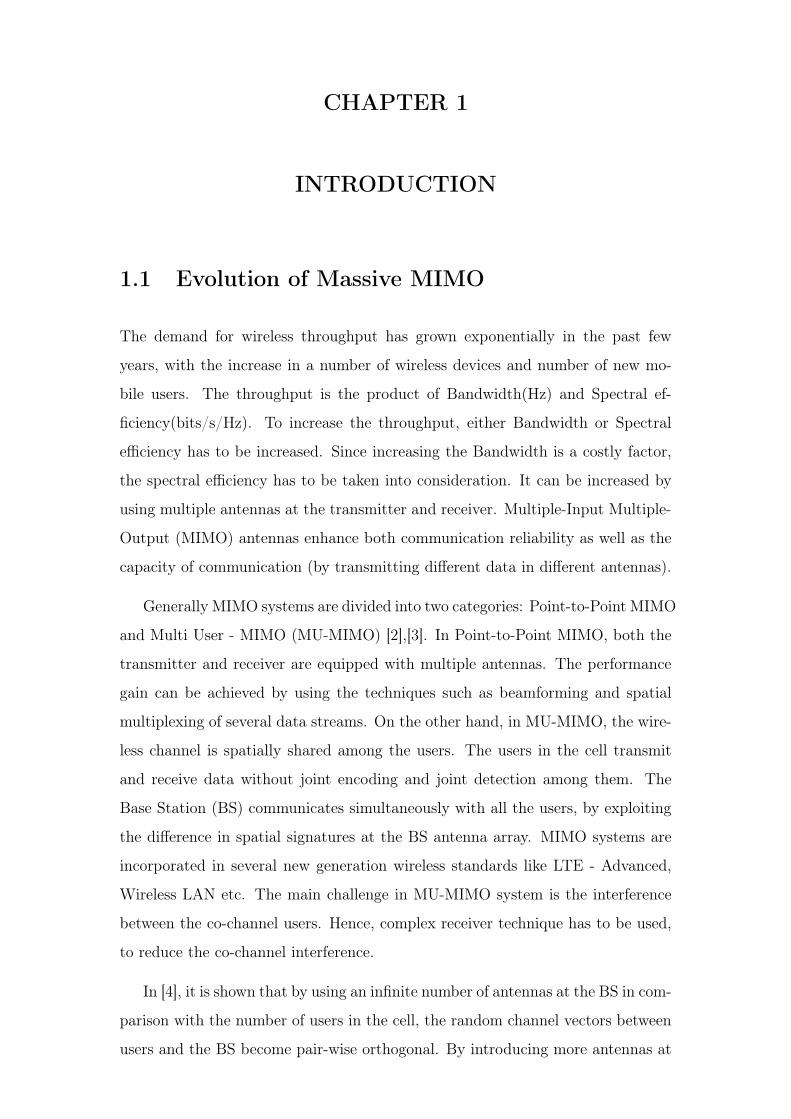
1.1 Evolution of Massive MIMO
The demand for wireless throughput has grown exponentially in the past few
years, with the increase in a number of wireless devices and number of new mo-
bile users. The throughput is the product of Bandwidth(Hz) and Spectral ef-
ficiency(bits/s/Hz). To increase the throughput, either Bandwidth or Spectral
efficiency has to be increased. Since increasing the Bandwidth is a costly factor,
the spectral efficiency has to be taken into consideration. It can be increased by
using multiple antennas at the transmitter and receiver. Multiple-Input Multiple-
Output (MIMO) antennas enhance both communication reliability as well as the
capacity of communication (by transmitting different data in different antennas).
Generally MIMO systems are divided into two categories: Point-to-Point MIMO
and Multi User - MIMO (MU-MIMO) [2],[3]. In Point-to-Point MIMO, both the
transmitter and receiver are equipped with multiple antennas. The performance
gain can be achieved by using the techniques such as beamforming and spatial
multiplexing of several data streams. On the other hand, in MU-MIMO, the wire-
less channel is spatially shared among the users. The users in the cell transmit
and receive data without joint encoding and joint detection among them. The
Base Station (BS) communicates simultaneously with all the users, by exploiting
the difference in spatial signatures at the BS antenna array. MIMO systems are
incorporated in several new generation wireless standards like LTE - Advanced,
Wireless LAN etc. The main challenge in MU-MIMO system is the interference
between the co-channel users. Hence, complex receiver technique has to be used,
to reduce the co-channel interference.
In [4], it is shown that by using an infinite number of antennas at the BS in com-
parison with the number of users in the cell, the random channel vectors between
users and the BS become pair-wise orthogonal. By introducing more antennas at
the BS, the effects of uncorrelated noise and intracell interference disappear and
small scale fading is averaged out. Hence, simple matched filter processing at BS
is optimal. MU-MIMO system with hundreds of antenna at the BS which serves
many single antenna user terminals simultaneously at same frequency and time is
known as Massive MIMO system or large antenna array MU-MIMO system [5],[6].
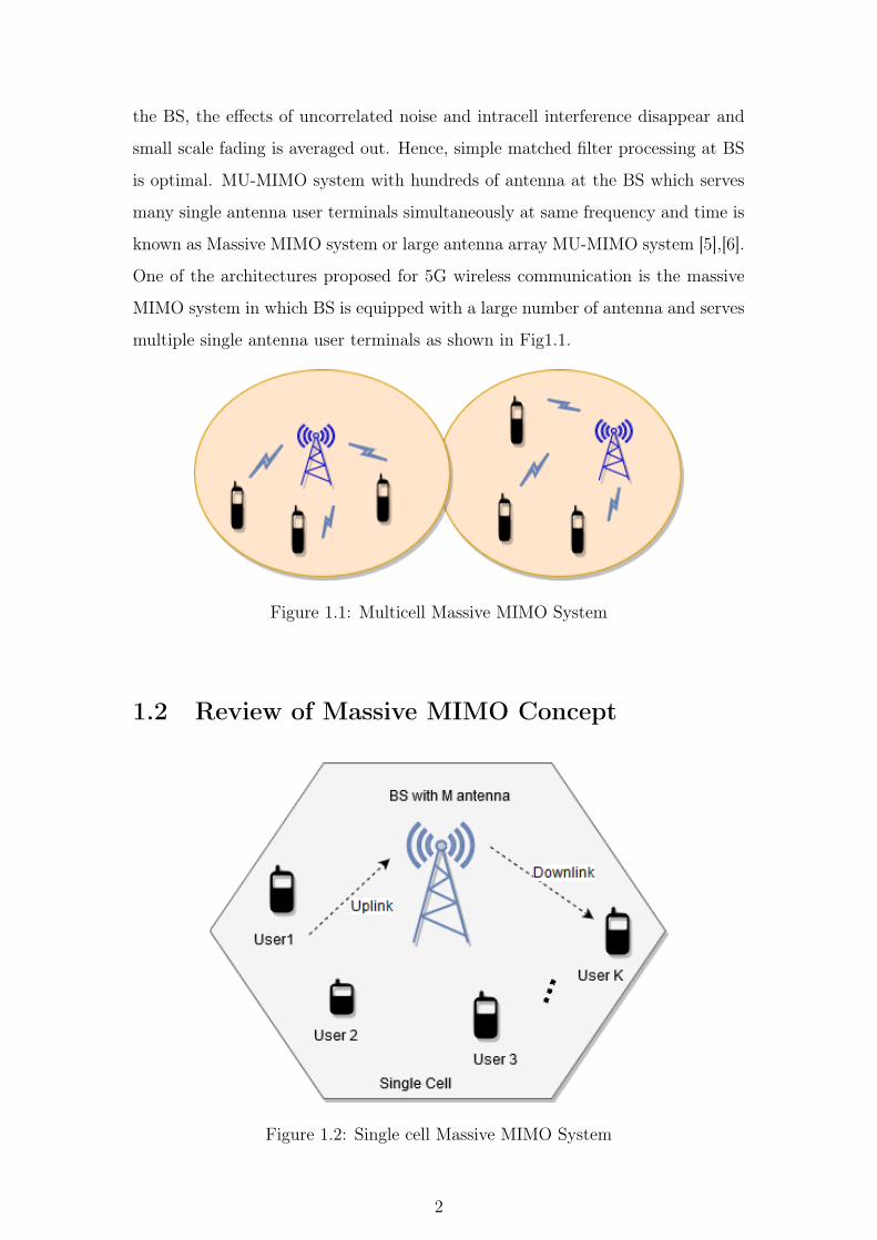
One of the architectures proposed for 5G wireless communication is the massive
MIMO system in which BS is equipped with a large number of antenna and serves
multiple single antenna user terminals as shown in Fig1.1.
Figure 1.1: Multicell Massive MIMO System
1.2 Review of Massive MIMO Concept
Figure 1.2: Single cell Massive MIMO System
2
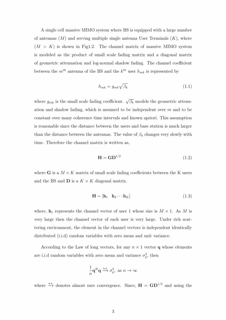
A single cell massive MIMO system where BS is equipped with a large number
of antennas (M) and serving multiple single antenna User Terminals (K), where
(M > K) is shown in Fig1.2. The channel matrix of massive MIMO system
is modeled as the product of small scale fading matrix and a diagonal matrix
of geometric attenuation and log-normal shadow fading. The channel coefficient
between the mth antenna of the BS and the kth user hmk is represented by
hmk = gmk
�βk (1.1)
where gmk is the small scale fading coefficient.√βk models the geometric attenu-
ation and shadow fading, which is assumed to be independent over m and to be
constant over many coherence time intervals and known apriori. This assumption
is reasonable since the distance between the users and base station is much larger
than the distance between the antennas. The value of βk changes very slowly with
time. Therefore the channel matrix is written as,
H = GD1/2 (1.2)
where G is a M ×K matrix of small scale fading coefficients between the K users
and the BS and D is a K ×K diagonal matrix.
H = [h1 h2 · · ·hK ] (1.3)
where, h1 represents the channel vector of user 1 whose size is M × 1. As M is
very large then the channel vector of each user is very large. Under rich scat-
tering environment, the element in the channel vectors is independent identically
distributed (i.i.d) random variables with zero mean and unit variance.
According to the Law of long vectors, for any n × 1 vector q whose elements
are i.i.d random variables with zero mean and variance σ2p, then
1
nqHq a.s−→ σ2
p, as n → ∞
where a.s−→ denotes almost sure convergence. Since, H = GD1/2 and using the
3
above law, by taking q as a column of G,
�HHHM
�
M�K
=
�D1/2G
HGM
D1/2
�
M�K
= D (from law of long vectors)
This shows that, the column vectors of the channel matrix are asymptotically
orthogonal. In similar way, to show orthogonality of row vectors:
�HHH
M
�
M�K
=
�G D1/2D1/2GH
M
�
M�K
=
�G DGH
M
�
M�K
=
�GGH
M
�D
M�K
= D (from law of long vectors)
This shows that, the row vectors of the channel matrix are asymptotically orthog-
onal.
1.2.1 Advantages of Massive MIMO System
• High energy efficiency: If the channel is estimated from the uplink pilots,
then each user’s transmitted power can be reduced proportionally to 1/√M
considering M is very large. If perfect Channel State Information (CSI) is
available at the BS, then the transmitted power is reduced proportionally to
1/M [7]. In the downlink case, the BS can send signals only in the directions
where the user terminals are located. By using the Massive MIMO, the
radiated power can be reduced achieving high energy efficiency.
• Huge Spectral efficiency: H defines the channel matrix between users
and BS. If we assume that perfect CSI is available at receiver, then from a
point-to-point Massive MIMO, the achievable rate is given by
C = log2 ||I +1
KHHH ||
bitss
Hz
4
The upper and lower bounds of the above equation can be derived as [3]
log2(1 +M) ≤ C ≤ min(M,K) log2(1 +max(M,K)
K) (1.4)
In Massive MIMO case, number of BS antennas is very large then (1.4)
becomes
C ≈ min(M,K) log2(1 +M
K)
bitss
Hz
The achievable rate is enhanced by a magnitude of approximately min(M,K)
than point-to-point MIMO case.
• Simple signal processing: Using an excessive number of BS antennas
compared to users lead to the pair-wise orthogonality of channel vectors.
Hence, with simple linear processing techniques both the effects of inter-
user interference and noise can be eliminated.
• Sharp digital beamforming : With an antenna array, generally analog
beamforming is used for steering by adjusting the phases of RF signals.
But in the case of Massive MIMO, beamforming is digital because of lin-
ear precoding. Digital beamforming is performed by tuning the phases and
amplitudes of the transmitted signals in baseband. Without steering actual
beams into the channels, signals add up in phase at the intended users and
out of phase at other users. With the increase in a number of antennas, the
signal strength at the intended users gets higher and provide low interfer-
ence from other users. Digital beamforming in massive MIMO provides a
more flexible and aggressive way of spatial multiplexing. Another advantage
of digital beamforming is that it does not require array calibration since
reciprocity is used.
• Channel hardening: The channel entries become almost deterministic in
case of Massive MIMO, thereby almost eliminating the effects of small scale
fading. This will significantly reduce the channel estimation errors.
• Reduction of Latency: Fading is the most important factor which impacts
the latency. More fading will leads to more latency. Because of the presence
of Channel hardening in Massive MIMO, the effects of fading will be almost
eliminated and the latency will be reduced significantly.
5
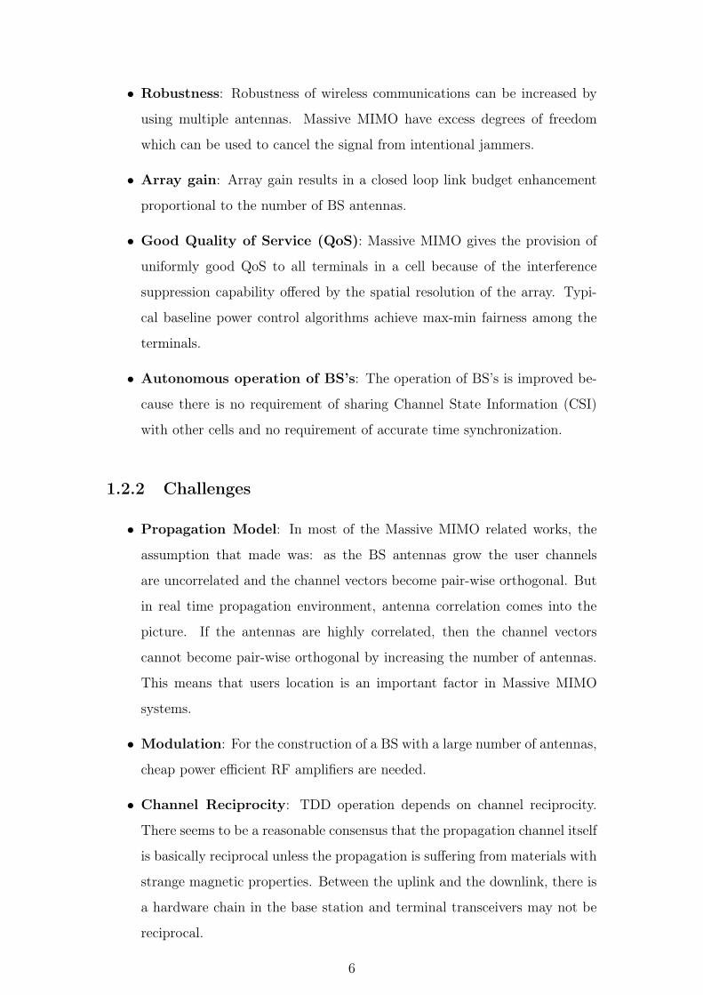
• Robustness: Robustness of wireless communications can be increased by
using multiple antennas. Massive MIMO have excess degrees of freedom
which can be used to cancel the signal from intentional jammers.
• Array gain: Array gain results in a closed loop link budget enhancement
proportional to the number of BS antennas.
• Good Quality of Service (QoS): Massive MIMO gives the provision of
uniformly good QoS to all terminals in a cell because of the interference
suppression capability offered by the spatial resolution of the array. Typi-
cal baseline power control algorithms achieve max-min fairness among the
terminals.
• Autonomous operation of BS’s: The operation of BS’s is improved be-
cause there is no requirement of sharing Channel State Information (CSI)
with other cells and no requirement of accurate time synchronization.
1.2.2 Challenges
• Propagation Model: In most of the Massive MIMO related works, the
assumption that made was: as the BS antennas grow the user channels
are uncorrelated and the channel vectors become pair-wise orthogonal. But
in real time propagation environment, antenna correlation comes into the
picture. If the antennas are highly correlated, then the channel vectors
cannot become pair-wise orthogonal by increasing the number of antennas.
This means that users location is an important factor in Massive MIMO
systems.
• Modulation: For the construction of a BS with a large number of antennas,
cheap power efficient RF amplifiers are needed.
• Channel Reciprocity: TDD operation depends on channel reciprocity.
There seems to be a reasonable consensus that the propagation channel itself
is basically reciprocal unless the propagation is suffering from materials with
strange magnetic properties. Between the uplink and the downlink, there is
a hardware chain in the base station and terminal transceivers may not be
reciprocal.
6

• Channel Estimation: To perform detection at the receiver side, we need
perfect CSI at the receiver side. Due to the mobility of users in MU case,
channel matrix changes with time. In high mobility case, accurate and time
acquisition of CSI is very difficult. FDD Massive MIMO induces training
overhead and TDD Massive MIMO relies on channel reciprocity and training
may occupy a large fraction of the coherence interval.
• Low-cost Hardware: Large number of RF chains, Analog-to-Digital con-
verters, Digital-to-Analog converters are needed.
• Coupling between antenna arrays: At the BS side, several antennas are
packed in a small space. This causes mutual coupling in between the antenna
arrays. Mutual coupling degrades the performance of Massive MIMO due
to power loss and results in lower capacity and less number of degrees of
freedom. When designing a Massive MIMO system, the effect of mutual
coupling has to be taken into account [8], [9].
• Mobility: If the mobility of the terminal is very high, then the coherence
interval between the channel becomes very less. Therefore, it accommodates
very less number of pilots.
• Pilot Contamination: Pilot contamination is a challenging problem for
multicell massive MIMO is to be resolved. In multicell system, users from
neighboring cells may use non-orthogonal pilots that result in pilot contami-
nation. This causes inter-cell interference problem which further grows with
the increase in a number of BS antennas. Various solutions suggested in the
literature to solve this problem for non cooperative cellular network are [10],
[11], [12], [13]:
– Channel Estimation Methods: These are based on some channel esti-
mation algorithm to detect the CSI by picking up the strongest channel
impulse responses, often done with less number of pilots than users.
– Time-Shifted Pilot Based Methods: These are based on insertion of
shifted pilot locations in slots (or a shifted frame structure).
– Optimum Pilot Reuse Factor Methods: These are based on choosing
a reuse factor greater than unity which is optimized in some sense.
7
In addition, there are significant performance gaps that exist among
different reuse patterns.
– Pilot Sequence Hopping Methods: These schemes switch users ran-
domly to a new pilot between time slots, which provides randomization
in the pilot contamination.
– Cell Sectoring based Pilot Assignment: These schemes are based on sec-
tioning the cells into a center and edge regions. Users in neighboring
border areas partly reuse sounding sequences. This improves the qual-
ity of service by reducing the number of serviced users. However, by
significantly reducing serviceable users, it degrades the system capacity.
1.3 Channel Estimation
In order to achieve the benefits of a large antenna array, accurate and timely acqui-
sition of Channel State Information (CSI) is needed at the BS. The need for CSI
is to process the received signal at BS as well as to design a precoder for optimal
selection of a group of users who are served on the same time-frequency resources.
The acquisition of CSI at the BS can be done either through feedback or channel
reciprocity schemes based on Time Division Duplex (TDD) or Frequency Division
Duplex (FDD) system. The procedure for acquiring CSI and data transmission
for both systems is explained in the subsequent sections.
1.3.1 Channel Estimation and Data Transmission in TDD
System
In TDD system, the signals are transmitted in the same frequency band for both
uplink and downlink transmissions but at different time slots. Hence, uplink and
downlink channels are reciprocal. During uplink transmission, all the users in the
cell synchronously send the pilot signal to the BS. The antenna array receives
the modified pilot signal by the propagation channel. Based on the received pilot
signal, BS estimate the CSI and further, this information is used to separate the
signal and detect the signal transmitted by the users as shown in Fig 1.3. In
8
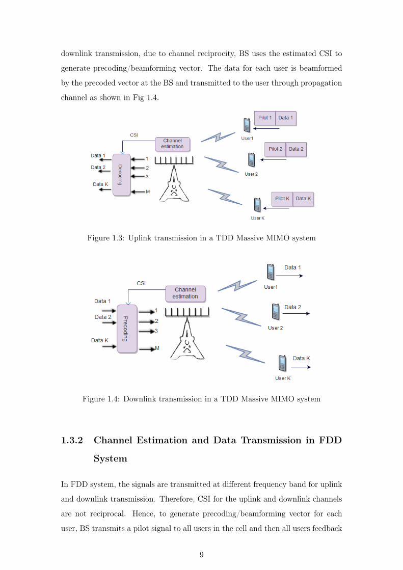
downlink transmission, due to channel reciprocity, BS uses the estimated CSI to
generate precoding/beamforming vector. The data for each user is beamformed
by the precoded vector at the BS and transmitted to the user through propagation
channel as shown in Fig 1.4.
Figure 1.3: Uplink transmission in a TDD Massive MIMO system
Figure 1.4: Downlink transmission in a TDD Massive MIMO system
1.3.2 Channel Estimation and Data Transmission in FDD
System
In FDD system, the signals are transmitted at different frequency band for uplink
and downlink transmission. Therefore, CSI for the uplink and downlink channels
are not reciprocal. Hence, to generate precoding/beamforming vector for each
user, BS transmits a pilot signal to all users in the cell and then all users feedback
9
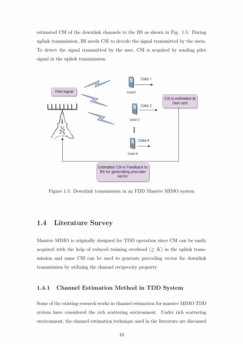
estimated CSI of the downlink channels to the BS as shown in Fig. 1.5. During
uplink transmission, BS needs CSI to decode the signal transmitted by the users.
To detect the signal transmitted by the user, CSI is acquired by sending pilot
signal in the uplink transmission.
Figure 1.5: Downlink transmission in an FDD Massive MIMO system
1.4 Literature Survey
Massive MIMO is originally designed for TDD operation since CSI can be easily
acquired with the help of reduced training overhead (≥ K) in the uplink trans-
mission and same CSI can be used to generate precoding vector for downlink
transmission by utilizing the channel reciprocity property.
1.4.1 Channel Estimation Method in TDD System
Some of the existing research works in channel estimation for massive MIMO TDD
system have considered the rich scattering environment. Under rich scattering
environment, the channel estimation technique used in the literature are discussed
10
below.
The authors in [14], proposed practical channel estimator to mitigate the prob-
lems caused by pilot contamination in multipath multicell massive MIMO TDD
systems. This practical estimator does not require knowledge of inter-cell large-
scale fading coefficients. Instead of individually estimating the large-scale coeffi-
cients, the proposed method estimates, a parameter that is the sum of large-scale
coefficients plus a normalized noise variance using minimum variance unbiased es-
timator. The estimated parameter is substituted back into the Bayesian MMSE
estimator without requiring any additional overhead.
In [15],[16] the conventional LS and MMSE estimation is proposed for channel
estimation problem. However, the problem is with the complexity of inverse which
is of order O(N 3) where N = MK. In order to overcome the inverse complexity,
in [16] a low complexity channel estimation using Polynomial expansion (PEACH
and W-PEACH) is proposed. In PEACH, an L-order matrix polynomial replaces
the inverse present in LS, MMSE, and Minimum Variance Unbiased estimation.
The problem with PEACH estimator is the complexity involved in finding out the
optimal weights.
In [17], partially decoded data is used to estimate the channel by which two
types of interference components, cross-contamination and self-contamination van-
ishes and they exist even when the number of antennas grows to infinity.
In massive MIMO system, blind channel estimation works well, since there is
unused degree of freedom in the signal space. One of the blind channel estima-
tion methods is the subspace portioning of the received samples. This method
can achieve near Maximum Likelihood performance when the data samples are
sufficiently large. In [18], Eigen Value Decomposition (EVD) based semi blind
channel estimation is proposed, considering the pilot sequences sent by the users
are orthogonal. CSI can be estimated from the Eigen vector of the covariance
matrix of the received samples, up to a multiplicative scalar factor ambiguity. By
using a short training sequence, this multiplicative factor ambiguity can be re-
solved. EVD-based channel estimation technique with the iterative least-square
projection algorithm is used to improve the performance of the channel estimation.
11
Recently, there has been a growing interest in compressive sensing (CS) based
channel estimation algorithms [19]. By exploiting the inherent sparsity of the
Massive MIMO channels, sparse channel estimation algorithms are proposed which
give better estimation performance than conventional schemes such as least square
and minimum mean square. In [20], the authors proposed a probability-weighted
subspace pursuit algorithm to estimate the channel. This method that estimates
the probabilities of the nonzero path delays in current Channel Impulse Response
(CIR) based on the knowledge of the previous CIR. The probability data is used
as a priori information in the subspace pursuit algorithm to improve the uplink
massive MIMO channel estimation.
In [21], the author modeled the channel estimation problem as a joint sparse
recovery problem . According to the block coherence property as the number of
antennas at the base station grows, the probability of joint recovery of the positions
of nonzero channel entries will increase. The block optimized orthogonal matching
pursuit is proposed to obtain an accurate channel estimate for the model.
1.4.2 Channel Estimation Method in FDD System
The CSI acquired in the uplink may not be accurate for the downlink due to the
calibration error of radio frequency chains and limited coherence time. More im-
portantly, compared with TDD systems, FDD systems can provide more efficient
communications with low latency. In FDD systems, CSI is obtained at every UT
by sending the pilot signal and the obtained CSI is fed back to the BS for precod-
ing. The number of orthogonal pilots required for downlink channel estimation
is proportional to the number of BS antennas, while the number of orthogonal
pilots required for uplink channel estimation is proportional to the number of
scheduled users. Therefore, to estimate the downlink channel, the pilot overhead
is in the order of a number of BS antenna which is prohibitively large in Massive
MIMO system and the corresponding CSI feedback is high overhead for uplink.
Therefore, it is of importance to explore channel estimation in the downlink than
that in the uplink, which can facilitate massive MIMO to be backward compatible
with current FDD dominated cellular networks. Hence it is necessary to explore
channel estimation method for massive MIMO based on FDD mode with reduced
12
overhead.
In order to overcome the excessive utilization of the resources in FDD mode,
considerable work have been done in downlink channel estimation and feedback
techniques. In recent, Compressed Sensing (CS) based channel estimation is con-
sidered for practical poor scattering channel [22]. CS is all about recovering the
sparse or compressible signal from limited number of measurements i.e., solving
the under-determined system [1], [23] and [24]. In most of the work, the propa-
gation medium in the virtual angular domain is considered as sparse based [25]
on the assumption the majority of channel energy is small due to the limited in
time-domain delay spread, angular spread, and Doppler domain. Hence downlink
channel estimation problem is formulated as a compressed sensing problem and
by utilizing the sparsity, the pilot overhead is reduced.
In [26], the block based orthogonal matching pursuit scheme is proposed for
downlink massive multiple-input single-output systems. In [27] the authors assume
that the path delays are invariant and utilize the channel support estimated from
the uplink training to enhance the downlink channel estimation using the Auxiliary
information based Block Subspace Pursuit algorithm.
The problem of CS is considered in two-dimensional (2D) sparse decomposition
measurement model in [28]. A modified 2D subspace pursuit algorithm is proposed
with the prior support and chunk sparse structure for the sparse channel estimation
in massive MIMO. In [29] along with sparsity, spatial correlation, and common
sparsity are assumed. By exploiting the channel block sparsity property, pilot
overhead is reduced and using Block-Partition CoSaMP (BP-CoSaMP) algorithm
downlink channel is estimated.
Standard sparse recovery algorithms have the stringent requirement on the
channel sparsity level for robust channel recovery and this severely limits the op-
erating regime of the solution. Therefore to overcome this issue, in [30] a joint
burst LASSO algorithm exploiting additional joint burst sparse structure is used.
In this method, the BS first transmits M pilots and then user feeds back the com-
pressed CSIT measurements to the BS. Finally, the joint burst LASSO algorithm
is performed at the BS based on the compressed CSIT measurements. Partial
Channel Support Information-aided burst Least Absolute Shrinkage and Selection
13
Operator (LASSO) algorithm is used to estimate the burst sparsity in massive
MIMO channels by exploiting both the partial channel support information and
additional structured properties of the sparsity in [31].
In Massive MIMO OFDM system, it has been proven that the equispaced
and equipower orthogonal pilots can be optimal to estimate the noncorrelated
Rayleigh MIMO channels for one OFDM symbol, where the required pilot over-
head increases with the number of transmit antennas [32]. By exploiting the spatial
correlation of MIMO channels, the pilot overhead to estimate MIMO channels can
be reduced. Furthermore, by exploiting the temporal channel correlation, further
reduced pilot overhead can be achieved to estimate MIMO channels associated
with multiple OFDM symbols [33] and [34]. In [35], a spectrum-efficient super-
imposed pilot signal occupy the same sub carriers in different transmit antenna
is used to estimate the channel with the help of the structured subspace pursuit
algorithm.
1.5 Motivation
In recent, CS based channel estimation is considered for practical poor scattering
channel [36] and it is all about recovering the sparse or compressible signal from
a limited number of measurements i.e., solving the under-determined system [1]
[23]. Sparse channel estimation is considered in many papers like in [25], where
they used inherent sparsity present in the channels (due to Doppler delay spread).
However in a situation like limited or poor scattering environment and non
zero antenna correlations at the BS end due to congested antenna spacing [37] [38],
causes the effective Degrees of Freedom (DoF) of the channel matrix to decrease,
which leads to decrease in the rank of the high dimensional channel matrix. The
advantages of massive MIMO is achieved if perfect CSI is known at the BS. To
estimate high dimensional channel matrix in poor scattering environment within
the coherence time interval is one of the big challenges.
In a finite scattering channel model, the number of AoAs is finite. In addition,
if the number of AoAs is less than the number of users, that would result in an
increase in the correlation between the channel vectors and a corresponding in-
14

crease in the condition number (or eigenvalue spread) of the channel matrix. In
this thesis, we considered the case when P < min{M,K} is fixed and therefore
the rank r of the channel matrix satisfies r < min{M,K,P}. Hence such a chan-
nel can conveniently be approximated as a low-rank channel. The conventional
Least Square (LS) approach fails to give the desired MSE performance under
such conditions. Therefore the channel estimation problem is modeled as a rank
minimization problem. Since the propagation medium considered is a low-rank
channel, it necessitates the development of the algorithm for obtaining low-rank
channel estimates.
The rank minimization problem is a nonconvex optimization problem and the
solution is NP hard to obtain. The nonconvex problem is approximated as con-
vex nuclear norm minimization problem [23] and is solved using Quadratic Semi-
Definite Programming (QSDP) approach [36] and [39]. This method is solved
using SDP solver and can provide the accurate result in the estimation only for a
matrix of size up to 100 × 100. Also, this method consume more time which will
not fit in the real time communication system. It is noted that the same problem
is solved using Iterative Singular Value Thresholding (ISVT) method [25]. How-
ever, the channel estimation using ISVT method gives a biased solution as all
singular values are penalized equally by the same threshold value. Since the larger
singular values contain the major information of the matrix will be lost by equal
penalization which leads the solution to deviate from the true singular values of
the channel matrix. This motivates to form the objective of the research as to
obtain unbiased low-rank channel estimates.
1.6 Contribution
The focus of this work is to estimate the channel for massive MIMO system under
limited scattering propagation environment. The channel is estimated under the
condition that the number of scatterers is small compared to the BS antennas
and number of users in the cell. If the number of scatterers is limited then the
corresponding Angle of Arrivals (AoAs) are finite. Moreover, if all the users share
the same AoAs then the correlation among the channel vector increases. Thus
15

the high dimensional channel matrix is approximated to the low-rank matrix.
Hence the objective of this thesis is to estimate the low-rank channel matrix. The
summary of the work done presented in the form of flowchart is given in Fig.1.6.
The contribution of the research work is listed below:
Figure 1.6: Flow chart showing the summary of the work done
1. Weighted Nuclear Norm Minimization (WNNM) method is proposed for low-
rank Massive MIMO channel estimation problem for both TDD and FDD
system.
2. Using Majorization and Minimization technique WNNM problem is solved
and low-rank channel matrix is obtained iteratively by the Weighted Singular
Value Thresholding algorithm.
3. Performance of the algorithm is analyzed by orthogonal and non-orthogonal
training sequence obtained by a restricted isometric property.
4. By using orthogonal training sequence, it is proved that the iterative algo-
rithm converges to one iteration.
5. For non-orthogonal training sequence, the algorithm takes more iteration to
converges. Hence to speed up the convergence rate, extra momentum term is
added in the algorithm and variable step size are used to reduce the number
16
of iteration. Hence, Fast Iterative Weighted Singular Value Thresholding
(FIWSVT) algorithm is proposed for channel estimation problem for the
non-orthogonal training sequence.
6. Regularization parameter is found in order to have low-rank property for the
resultant estimated channel matrix.
7. The significance of the proposed channel estimation problem in TDD is an-
alyzed through the Mean Square Error and Average Sum Rate (uplink and
downlink mode) as the performance index and are compared with the Nu-
clear Norm method using different scatterers.
8. The WNNM method is also extended to FDD mode by modeling the down-
link FDD channel as low rank and uplink channel as the full rank matrix.
Both downlink and uplink channel are estimated at BS. The performance of
the FIWSVT algorithm for estimating downlink low-rank channel in FDD
mode is analyzed through the Mean Square Error. The results are compared
with the existing SVP-G, SVP-N, and SVP-H algorithm.
1.7 Thesis Organization
The rest of the thesis is organized as follows. Chapter 2 presents the modeling
of finite scattering channel for single cell system as a low rank. System model
used in the rest of the thesis and the different performance metrics used to study
the performance of the algorithms are described. The failure of conventional least
square method to estimate low-rank channel is explained. The existing method-
ology already used to estimate the low-rank channel matrix and their advantages
and disadvantages are presented. The WNNM method proposed to estimate the
low-rank matrix is discussed. The majorization and minimization technique used
to solve WNNM method is presented.
Chapter 3 focus on the performance analysis of Iterative Weighted Singular
Value Threshold channel estimation algorithm using non-orthogonal training se-
quence. The selection of training matrix using restricted isometric property is
presented. The different weight function used in the analysis of the algorithm is
17

discussed. The convergence analysis of the iterative algorithm with non-orthogonal
training sequence is studied. The increase in the convergence speed of the iterative
algorithm by introducing the momentum function in the algorithm is presented.
The estimation of the regularization parameter in order to achieve low-rank ma-
trix is discussed. The performance and the convergence analysis of the algorithm
are tested for a different number of scatterers and signal to noise ratio. The per-
formance analysis of the algorithm is also validated by varying the number of BS
antenna and the number of users in the cell is presented.
Chapter 4 deals with the performance study of WNNM method using orthog-
onal training sequence. The selection of training matrix using restricted isometric
property is presented. Convergence analysis of the iterative algorithm with or-
thogonal training sequence is studied. The selection of regularization parameter
in order to achieve low-rank matrix and the selection of weights for WNN method
are discussed. In order to obtain minimum mean square error, the selection of tun-
ing parameter using Stein’s unbiased risk estimate is studied. The performance
and the convergence analysis of the algorithm are tested for a different number of
scatterers and signal to noise ratio and validated by varying the number of base
station antennas and the number of users in the cell is presented.
Chapter 5 presents the issue related to the implementation of the massive
MIMO in FDD system. The modeling of the FDD downlink channel as a low-
rank matrix and uplink as the full rank is discussed. The downlink low-rank
channel and the uplink full rank channel is jointly estimated at BS is presented.
The proposed WNNM method is presented for estimating channel at BS. The
performance of the algorithm in FDD mode is tested for non-orthogonal training
matrix. The convergence analysis of the proposed FIWSVT algorithm is compared
with the existing algorithms like Singular Value Projection(SVP)-Gradient, SVP-
Newton and SVP-Hybrid algorithm. The comparison of normalized mean square
error performance is compared with the FISVT algorithm for different uplink SNR
levels are presented.
Chapter 6 presents the conclusions from the work presented in this thesis.
Possible future extensions are also discussed.
18
CHAPTER 2
Finite Scattering Channel Model and Low-Rank
Channel Estimation
2.1 Introduction
In this chapter finite scattering propagation environment for massive MIMO is
modeled in Section 2.2. When the number of scatterers is very small compared to
the number of base station antennas which is in the order of hundreds and number
of users in the cell which is in tens and if the same scatterers are shared by all
users, then the correlation among the channel vectors of users increases. Hence,
the high dimensional MIMO system is likely to approximate the channel matrix
as low rank. In this chapter, different methodology used to estimate the low-rank
channel, their advantages and disadvantages are discussed.
In Section 2.3, the model of the massive MIMO system operating in TDD mode
is described. The conventional Least Square (LS) method to estimate channel ma-
trix is explained during the initial phase. The failure of LS to achieve low-rank fea-
ture in the estimated channel matrix is outlined. In order to overcome the failure
of the conventional method, the low-rank channel matrix estimation is formulated
as the Nuclear Norm Minimization (NNM) problem. The solution for solving the
minimization problem using the Majorization and Minimization (MM) technique
is discussed and the algorithm for estimation is outlined. To overcome the biased
solution provided NNM method, the rank minimization problem is formulated as
the Weighted Nuclear Norm minimization (WNNM) problem and further, the al-
gorithm for the optimization problem is discussed. The performance metrics are
used to analyze the proposed channel estimation algorithm are described.
2.2 Finite Scattering Channel Model for Single Cell
in TDD System
In finite scattering channel model, the propagation is modeled in terms of a finite
number of multiple path components [40], [41], and [42]. Each path is specified by
AoA, complex gain, and delay. Delay of each path is neglected, since narrow band
system is considered. The following assumptions are made regarding the channel
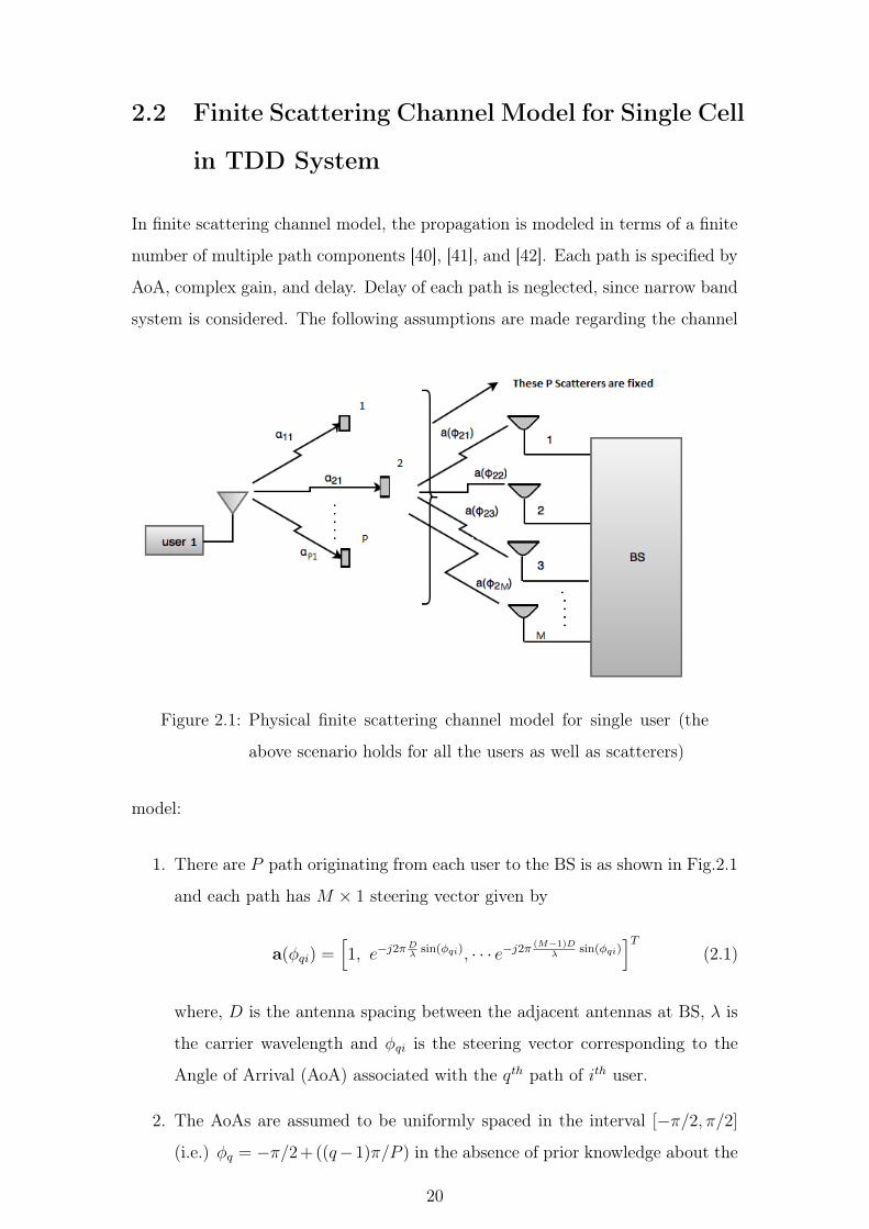
Figure 2.1: Physical finite scattering channel model for single user (the
above scenario holds for all the users as well as scatterers)
model:
1. There are P path originating from each user to the BS is as shown in Fig.2.1
and each path has M × 1 steering vector given by
a(φqi) =�1, e−j2πD
λsin(φqi), · · · e−j2π
(M−1)Dλ
sin(φqi)�T
(2.1)
where, D is the antenna spacing between the adjacent antennas at BS, λ is
the carrier wavelength and φqi is the steering vector corresponding to the
Angle of Arrival (AoA) associated with the qth path of ith user.
2. The AoAs are assumed to be uniformly spaced in the interval [−π/2, π/2]
(i.e.) φq = −π/2+((q−1)π/P ) in the absence of prior knowledge about the
20
distribution of AoAs and each path is indexed by an integer q ∈ [1, 2 · · ·P ].
3. There are fixed number of scatterers (P ) distributed within the cell.
Therefore the channel vector of the ith user to the BS is modeled as a linear
combination of the P steering vectors
hi =1√P
P�
q=1
αqia(φqi)) (2.2)
where, αqi ∼ CN (0, 1) is the path gain of the qth path to the ith user. In vector
form the channel vector of ith user is represented as
hi = Aigi (2.3)
where the AoAs matrix Ai is given as
Ai =1√P
1 1 . . . 1
e−j2πDλsin(φ1i) e−j2πD
λsin(φ2i) . . . e−j2πD
λsin(φPi)
e−j2π 2Dλ
sin(φ1i) e−j2π 2Dλ
sin(φ2i) . . . e−j2π 2Dλ
sin(φPi)
...... . . . ...
e−j2π(M−1)D
λsin(φ1i) e−j2π
(M−1)Dλ
sin(φ2i) . . . e−j2π(M−1)D
λsin(φPi)
If there are P fixed scatterers around each individual users who are geographi-
cally separated in the cell as shown in the Fig.2.2, then the steering matrix for
each individual user will be different. Therefore the channel matrix M ×K com-
bining all users in the cell is represented as
H = [A1g1,A2g2, · · ·AKgK] (2.4)
where the A1 is M × P steering matrix of user 1. In this case, the rank of the
channel matrix r = min{M,K,P}.
2.2.1 Channel Model with Identical AoAs
In this thesis, we have considered the case, if there are P fixed scatterers around
the BS and all users who are geographically separated in the cell are accessible
to the P scatterers as shown in Fig. 2.3. Under this condition all users will have
21
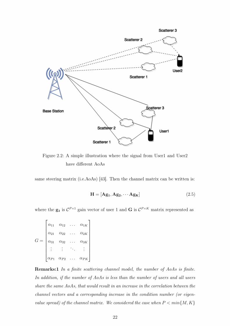
Figure 2.2: A simple illustration where the signal from User1 and User2
have different AoAs
same steering matrix (i.e.AoAs) [43]. Then the channel matrix can be written is:
H = [Ag1,Ag2, · · ·AgK] (2.5)
where the g1 is CP×1 gain vector of user 1 and G is CP×K matrix represented as
G =
α11 α12 . . . α1K
α21 α22 . . . α2K
α31 α32 . . . α3K
...... . . . ...
αP1 αP2 . . . αPK
Remarks:1 In a finite scattering channel model, the number of AoAs is finite.
In addition, if the number of AoAs is less than the number of users and all users
share the same AoAs, that would result in an increase in the correlation between the
channel vectors and a corresponding increase in the condition number (or eigen-
value spread) of the channel matrix. We considered the case when P < min{M,K}
22
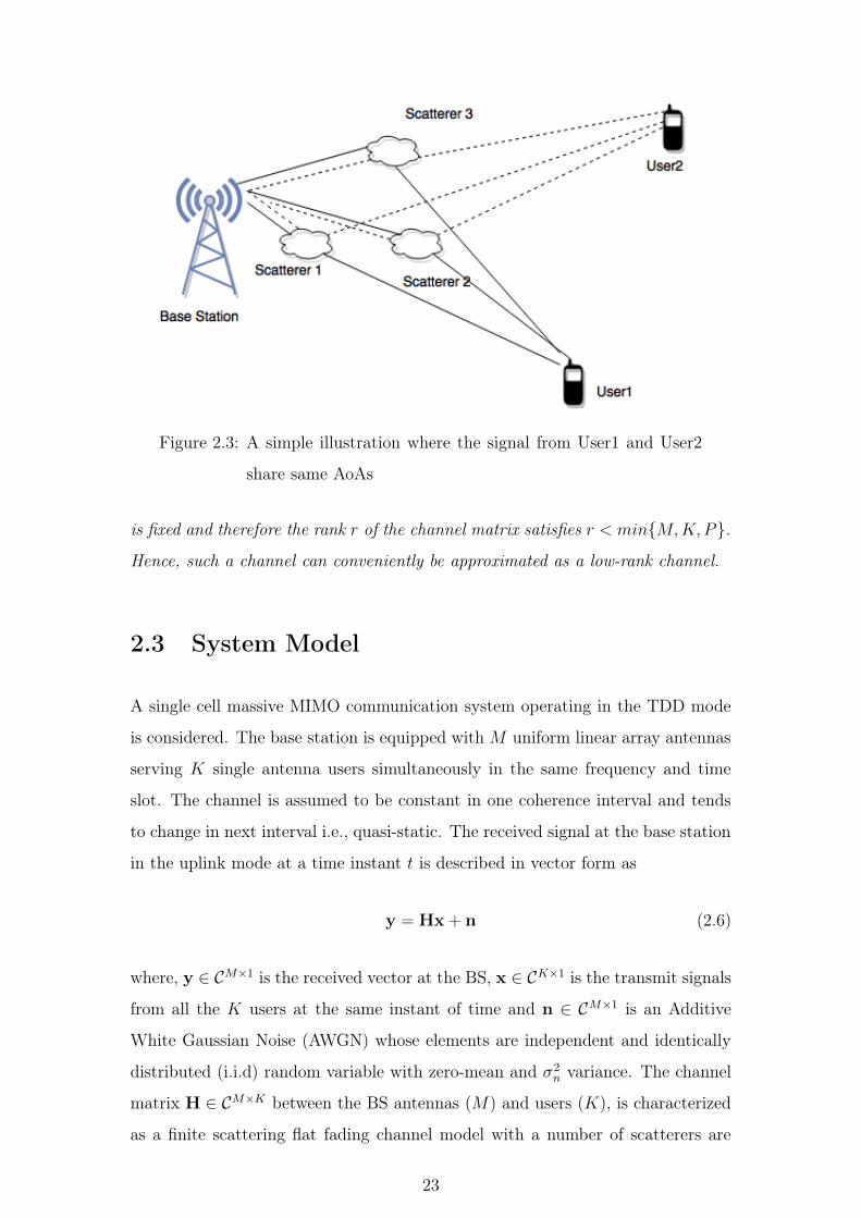
Figure 2.3: A simple illustration where the signal from User1 and User2
share same AoAs
is fixed and therefore the rank r of the channel matrix satisfies r < min{M,K,P}.Hence, such a channel can conveniently be approximated as a low-rank channel.
2.3 System Model
A single cell massive MIMO communication system operating in the TDD mode
is considered. The base station is equipped with M uniform linear array antennas
serving K single antenna users simultaneously in the same frequency and time
slot. The channel is assumed to be constant in one coherence interval and tends
to change in next interval i.e., quasi-static. The received signal at the base station
in the uplink mode at a time instant t is described in vector form as
y = Hx+ n (2.6)
where, y ∈ CM×1 is the received vector at the BS, x ∈ CK×1 is the transmit signals
from all the K users at the same instant of time and n ∈ CM×1 is an Additive
White Gaussian Noise (AWGN) whose elements are independent and identically
distributed (i.i.d) random variable with zero-mean and σ2n variance. The channel
matrix H ∈ CM×K between the BS antennas (M) and users (K), is characterized
as a finite scattering flat fading channel model with a number of scatterers are
23
less than the number of BS antennas and number of user in the cell. We have also
assumed that all the users in the cell share the same scatterers which approximate
the high dimensional channel matrix as the low-rank matrix.
The propagation medium is considered as a low-rank channel, therefore, it
necessitates the development of an algorithm for obtaining low-rank channel esti-
mates. The subsequent sections deal with the different methods to estimate the
low-rank channel matrix.
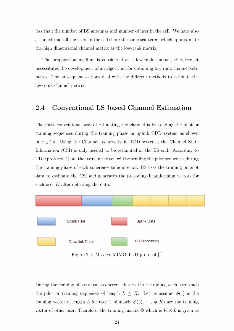
2.4 Conventional LS based Channel Estimation
The most conventional way of estimating the channel is by sending the pilot or
training sequences during the training phase in uplink TDD system as shown
in Fig.2.4. Using the Channel reciprocity in TDD systems, the Channel State
Information (CSI) is only needed to be estimated at the BS end. According to
TDD protocol [1], all the users in the cell will be sending the pilot sequences during
the training phase of each coherence time interval. BS uses the training or pilot
data to estimate the CSI and generates the precoding/beamforming vectors for
each user K after detecting the data.
Figure 2.4: Massive MIMO TDD protocol [1]
During the training phase of each coherence interval in the uplink, each user sends
the pilot or training sequences of length L ≥ K. Let us assume φ(1) is the
training vector of length L for user 1, similarly φ(2), · · · , φ(K) are the training
vector of other user. Therefore, the training matrix Φ which is K × L is given as
24
Φ = [φ(1)T ,φ(2)T · · ·φ(K)T ]. The received signal at the BS Y ∈ CM×L is given
by:
Y = HΦ+N (2.7)
where N is AWGN matrix with i.i.d entries of CN (0, 1). Since, no statistical
knowledge about channel is assumed, the LS channel estimates minimize the mean
square error given by minimizing:
minH
�Y −HΦ�2F
The solution to the unconstrained problem is given as:
HLS = YΦ† = YΦH(ΦΦH)−1 (2.8)
The LS method estimates the channel based on the received and transmitted
training sequences by minimizing the mean square error. The main drawback of
LS estimation is that it does not impose the low-rank feature of the channel matrix
in the cost function. Moreover, the computational complexity of LS method is in
the order of O(N 3) where N = MK. In order to overcome the limitation of LS
estimates, the problem of low-rank channel estimates is proposed and details are
discussed in the following section.
2.5 Low-Rank Channel Estimation
2.5.1 Nuclear Norm Minimization Method
In the finite scattering propagation environment, the channel matrix exhibit low-
rank feature and the conventional Least Square (LS) approach to estimate the
channel fail to provide the desired rank of the channel matrix. Therefore, to
estimate the channel at the receiver, the channel estimation problem can be for-
mulated as a linearly constrained rank minimization problem [25]:
minH
rank(H) s.t. Y = HΦ (2.9)
25
The constrained equation shown in equation (2.9) is obtained by applying the
vectorization formula to the received signal matrix using Lemma 2.5.1.
Lemma 2.5.1 The vectorization of an M × K matrix A, denoted by vec(A),
is the MK × 1 column vector obtained by stacking the columns of the matrix A
on top of one another. If A ∈ CM×K and B ∈ CK×L are two matrix, then the
vectorization of product of two matrices is vec(AB) = (BT ⊗ IM)vec(A).
Therefore, (2.9) can be written as
minH
rank(H) s.t. y = Ψh (2.10)
where y = vec(Y), h = vec(H), and Ψ = (ΦT ⊗ IM).
Rank minimization problem is a nonconvex optimization problem and is com-
putationally intractable (NP-hard). Also, there are no efficient exact algorithms
to solve the problem. The convex envelope of the rank function which is equivalent
to the nuclear norm is a tractable convex approximation that can be minimized
efficiently (A.1). Hence, the constrained rank minimization is approximated as
the constrained NNM problem.
minH
�H�∗ =r�
i=1
σi
s.t. y = Ψh
(2.11)
where r indicate the desired rank of the channel matrix. In order to solve this
problem rank information should be known prior and the optimization problem can
be solved iteratively using hard Thresholding algorithm [44] [45]. However, it is
difficult to obtain the prior information about the rank of the channel. Therefore,
without providing the rank information we can estimate the low-rank channel by
reformulating the constrained nuclear norm minimization problem (2.11) as an
unconstrained minimization problem given as:
minH
1
2||y −Ψh)||22 + λ||H||∗ (2.12)
The term 12||y−Ψh)||22 in (2.12) is known as loss function and the term λ||H||∗ is
26

called regularizer function. This nuclear norm minimization problem can be refor-
mulated as Quadratic Semi Definite Programming (QSDP) [46] problem and can
be solved efficiently. However, QSDP approach will not fit in real time communi-
cation system due to time complexity. Moreover, it provides accurate results for
the matrix of size up to 100 × 100. The same problem can be solved heuristically
using Majorization - Minimization technique.
2.5.1.1 Majorization - Minimization Technique
The Majorization - Minimization (MM) technique [47], [48] is a simple optimiza-
tion principle used for minimizing an objective function (2.12) written as
J(h) =1
2||y −Ψh)||22 + λ||H||∗ (2.13)
The first term in the cost function is the convex and smooth function where as
the nuclear norm is a convex and nonsmooth function. Hence the resultant cost
function is convex and nonsmooth. Instead of directly minimizing the cost function
(2.13), the principle used by the MM technique is shown in Fig.2.5 to solve (2.13)
is as follows:
Figure 2.5: Illustration of Majorization-Minimization technique
1. Find the majorizing surrogate function Gk(h) for the cost function J(h) that
27
coincides with J(h) at h = hk and upper bound J(h) at all other value of h
i.e, finding the surrogate function Gk(h) that lies above the surface of J(h)
and is tangent to J(h) at the point h = hk which is mathematically defined
as
Gk(h/hk) ≥ J(h) ∀h (2.14)
Gk(hk/hk) = J(hk) h = hk
2. Compute the surrogate function at each iteration and further update the
current estimate.
This successive minimization of the majorizing function Gk(h) ensures that the
cost function J(h) decreases monotonically. This guarantees global convergence
for convex cost function.
The competence of MM technique depends on how well the surrogate approximate
J(h). The quadratic surrogate function Gk(h) can well approximate the convex
nonsmooth function so that it satisfies the condition (2.14).
Gk(h) = J(h) + non negative function of h (2.15)
and the non-negative function chosen is 12(h − hk)
H(αI −ΨHΨ)(h − hk). Thus,
Gk(h) = J(h) +1
2(h − hk)
H(αI −ΨHΨ)(h − hk) + λ||H||∗ (2.16)
At h = hk, Gk(h) coincides with J(h). To ensure the added term to be a non-
negative for all value of h, choose α > σmax(ΨHΨ)) and for convex function
h ≤ hk. Hence, the added term is non negative for all h value.
To minimize the majorizer function Gk(h), differentiate Gk(h) with respect to h
and equate to zero. Therefore, the equation (2.16) would become
h = hk +1
αΨH(y −Ψhk) (2.17)
The vector h is computed iteratively, by upgrading the equation ( 2.17)
hk = hk−1 +1
αΨH(y −Ψhk−1) (2.18)
28
By substituting (2.18) in (2.16), Gk(h) can be written as
Gk(h) =α
2||h− hk||22 − hk
Hhk + yHy+ hk−1H(α−ΨHΨ)hk−1 + λ||H||∗ (2.19)
It is observed from (2.19) that, only first and last term depends on h and all
other terms are independent of h. Therefore, instead of minimizing Gk(h), we can
minimize
Gk(h) =1
2||h − hk||22 + ν||H||∗
where, h = vec(H), hk = vec(Hk) and ν = λ/α
||h − hk||22 = ||H −Hk||2F
[49]. Therefore, the cost function to be minimized can be written as
minH
ν||H||∗ +1
2||H −Hk||2F (2.20)
Theorem 2.5.1.1 For any λ > 0, Y ∈ CM×K then the following problem
minX
1
2||Y−X||2F + λ||X||∗ (2.21)
is the convex optimization problem and the closed form solution is X∗ = USλ(Σ)VH
where Y = UΣVH is the SVD of Y and Sλ(Σ) = Diag{(σi − λ)+} is the soft
thresholding done on the ith singular value σi where, x+ denotes max(x, 0).
Proof:
For any X,Y ∈ CM×K , the singular value decomposition of matrix X and Y are de-
noted by U S VH
and UΣVH respectively, where Σ = diag {σ1, σ2, · · · σK , 0 · · · , 0} ∈RM×K and S = diag {s1, s2, · · · sK , 0 · · · , 0} ∈ RM×K are the diagonal singular
value matrices such that s1 > s2 > · · · > sk ≥ 0 and σ1 > σ2 > · · · > σK ≥ 0.
The following derivations hold based on Frobenius norm:
minX
1
2||Y − X||2F + λ||X||∗ (2.22)
= minX
1
2[Tr(YHY)− 2Tr(YHX) + Tr(XHX)] + λ
K�
i=1
si
29
if U = U and V = V
= minS
1
2[
K�
i=1
σ2i − 2
K�
i=1
σisi +K�
i=1
s2i ] + λ
K�
i=1
si
= minS
1
2[
K�
i=1
(si − σi)2] + λ
K�
i=1
si
for a particular i, the equation can be written as
minsi≥0
f(si) =1
2(si − σi)
2 + λsi
To find si, take the derivative of f(si) and equate to zero
f �(si) = si − σi + λ = 0
then
si = max(σi − λ, 0), i = 1, 2, ....K (2.23)
Since σ1 ≥ σ2 ≥ · · · ≥ σK then s1 ≥ s2 ≥ · · · ≥ sK . Thus, the global optimum
solution to NN problem is the soft thresholding operator on the singular value of
the matrix Y which is given as
X∗ = USλVH
where, Sλ = Diag{(σi − λ)+} is the soft thresholding done on the singular value.
Based on Theorem 2.5.1.1, the solution to the minimization problem Gk is
H∗ = USν(Σ)VH where, U and V are obtained from the Singular Value Decom-
position (SVD) of HK (where HK is equivalent to Y in the theorem).
Therefore, the channel matrix is estimated by computing the following three equa-
tions iteratively:
Hk = Hk−1 +1
αvec_matM,K(Ψ
Hvec(Y −Hk−1Φ))
Hk = UΣVH
H∗ = USν(Σ)VH
30

The explanation behind the updates of the equation is as follows:
1. The current update of the channel matrix is obtained by updating the previ-
ous channel estimates in the gradient direction evaluated from loss function
at a fixed step size of 1α.
2. In order to obtain the low rank solution to the estimates, the updated matrix
is projected on to the low-rank matrix constraint set. This projection is
done using SVD and soft thresholding operator on the singular value of the
updated matrix.
3. The soft thresholding rule makes any singular values less than the threshold
value is set to zero to have reduced rank channel matrix.
The algorithm used to iteratively solve the set of equations for the channel estima-
tion problem is called as Iterative Singular Value Thresholding (ISVT) algorithm
[50].
2.5.1.2 Iterative Singular Value Thresholding algorithm
In this section, the Iterative Singular Value Thresholding (ISVT) algorithm being
adapted to the channel estimation problem is described.
Algorithm : Iterative Singular Value Thresholding algorithm
1: Input M,K,L, Φ, Y, λ, α, ν = λ/α
2: Initialization: H(1) = 0,Ψ = ΦT ⊗ IM
3: Until ||H(i)−H(i+1)||F||H(i+1)||F < δ
4: A ← H(i) + 1αvec_matM,K(Ψ
Hvec(Y − H(i)Φ))
5: [UΣV] = SV D(A)
6: Thresholding : Sν(Σ) = Diag(σi − ν)
7: H(i+ 1) ← USν(Σ)VH
31
8: i ← i+ 1
9: Go to 3
10: Output: H(i+ 1)
The initial value of the channel matrix is assumed as zero matrix. At each it-
eration, the channel matrix is gets updated using the equation given in step 4.
In order to get the low rank solution to the estimated channel matrix, in each
iteration soft thresholding is done according to the equation in step 6. These
steps are executed iteratively until the normalized difference between the previous
estimates and current estimates reaches the threshold δ.
2.5.1.3 Complexity Order
The main computational complexity lies in calculating SVD of the M×K matrix,
which has a complexity of O(M 2K) (at each iteration). The matrix-vector mul-
tiplication in step (4) has a complexity of O((ML)(MK)). The total complexity
of the ISVT algorithm is O(iter(M 2K + (ML)(MK))), where iter is the number
of iteration required to obtain the desired result.
Remarks 2: The soft thresholding scheme which is used in ISVT algorithm
Sλ(Σ) = Diag{(σi − λ)+} ignores the prior knowledge about the singular values.
The soft thresholding scheme penalize the larger singular values as heavily as the
lower ones by the threshold or regularizer λ, which deviate the solution from the
true singular value of the channel matrix. In comparison with the small singular
values, the larger ones are generally associated with the major information of the
channel matrix. Hence, it should be shrunk less compared to lower ones. Therefore,
different weights to different singular values overcome the limitation of NN method.
32
2.5.2 Weighted Nuclear Norm Minimization Method
To overcome the above issues, the problem stated in (2.12) can be relaxed by
the nonconvex regularizer. The nonconvex regularizer function proposed in this
section is the WNN and hence the optimization problem can be redefined as:
minH
1
2||y −Ψh||22 + λ||H||w,∗ (2.24)
where, ||H||w,∗ = ΣKi=1wiσi.
In general, WNN is a nonconvex regularizer. However, if the weights satisfy
the condition 0 ≤ w1 ≤ w2 ≤ · · · ≤ wK then σ1w1 ≥ σ2w2 ≥ σ3w3 ≥ · · · ≥ σKwK .
Therefore, the resultant singular values are arranged in a non-increasing order
which is same as the nuclear norm and hence satisfy the convexity. Therefore, by
applying the same principle of Majorization and Minimization technique to the
above problem results in minimization of the cost function
minH
ν||H||w,∗ +1
2||H −Hk||2F (2.25)
whose solution is presented in Theorem 2.5.2.1.
Theorem 2.5.2.1 For any λ > 0, Y ∈ CM×K and if the weights to the singular
values satisfy the condition 0 ≤ w1 ≤ w2 ≤ · · · ≤ wK then the following problem
minX
1
2||X−Y||2F + λ||X||w,∗ (2.26)
is the convex optimization problem and the closed form solution to this problem
is X∗ = USλ,wVH where Y = UΣVH is the SVD of Y and Sλ,w = Diag{(σi −λwi)+} is the weighted soft thresholding done on the singular value.
Proof:
For any X,Y ∈ CM×K , the singular value decomposition of matrix X and Y are de-
noted by U S VH
and UΣVH respectively, where Σ = diag {σ1, σ2, · · · σK , 0 · · · , 0} ∈RM×K and S = diag {s1, s2, · · · sK , 0 · · · , 0} ∈ RM×K are the diagonal singular
value matrices such that s1 > s2 > · · · sk ≥ 0 and σ1 > σ2 > · · · > σK ≥ 0. The
33
following derivations hold based on Frobenius norm:
minX
1
2||Y − X||2F + λ||X||w,∗ (2.27)
= minX
1
2[Tr(YHY)− 2Tr(YHX) + Tr(XHX)] + λ
K�
i=1
wisi
if U = U and V = V
= minS
1
2[
K�
i=1
σ2i − 2
K�
i=1
σisi +K�
i=1
s2i ] + λK�
i=1
wisi
= mins
1
2[
K�
i=1
(si − σi)2] + λ
K�
i=1
wisi
for a particular i, the equation can be written as
minsi≥0
f(si) =1
2(si − σi)
2 + λwisi
To find si, take the derivative of f(si) and equate to zero
f �(si) = si − σi + λwi = 0
then
si = max(σi − λwi, 0), i = 1, 2, · · · , K (2.28)
Since σ1 ≥ σ2 ≥ · · · ≥ σK and by choosing the weight vector in a non-descending
order w1 ≤ w2 ≤ · · ·wK , then si will satisfy the condition s1 ≥ s2 ≥ · · · ≥sK . Thus, the global optimum solution to WNN problem is the weighted soft
thresholding operator on the singular value of the matrix Y which is given as
X∗ = USλ,wVH
where, Sλ,w = Diag{(σi − λwi)+} is the weighted soft thresholding done on the
singular value.
Based on Theorem 2.5.2.1, the solution to the minimization problem is H∗ =
USν,wVH where, U and V are obtained from the SVD of Hk (where HK is equiv-
alent to Y in the theorem).
34
Therefore, the channel matrix is estimated by computing the following three equa-
tion iteratively:
Hk = Hk−1 +1
αvec_matM,K(Ψ
Hvec(Y −Hk−1Φ))
Hk = UΣVH
H∗ = USν,w(Σ)VH
This set of equations used to solve the channel estimation problem is called as
Iterative Weighted Singular Value Thresholding (IWSVT) algorithm.
2.5.2.1 Iterative Weighted Singular Value Thresholding Algorithm
The Iterative Weighted Singular Value Thresholding (IWSVT) algorithm being
adapted to the channel estimation problem is described below.
Algorithm : Iterative Weighted Singular Value Thresholding Algorithm
1: Input M,K,L, Φ, Y, λ, α
2: Initialization: H(1) = 0,Ψ = ΦT ⊗ IM
3: Until ||H(i)−H(i+1)||F||H(i+1)||F < δ
4: A ← H(i) + 1αvec_matM,K(Ψ
Hvec(Y − H(i)Φ))
5: [UΣV] = SV D(A)
6: Update the weight function wi
7: Thresholding : Sν,w(Σ) = Diag(σi − νwi)
8: H(i+ 1) ← USν,w(Σ)VH
9: i ← i+ 1
10: Go to 3
11: Output: H(i+ 1)
35
The channel matrix is initially assigned as zero matrix. At each iteration, the
channel matrix is getting updated using the equation given in step 4. The weight
for each singular values is computed, based on the singular values obtained from
the SVD of the matrix in step 4. In order to get a low rank solution to the estimated
channel matrix, in each iteration weighted soft thresholding is done according to
the equation in step 7. These steps executed iteratively until the normalized differ-
ence between the previous estimates and current estimates reaches the threshold
δ.
2.5.2.2 Complexity Order
The computational complexity of IWSVT algorithm is same as ISVT algorithm.
The total complexity of the IWSVT algorithm is O(iter(M 2K + (ML)(MK))).
2.6 Performance Metrics
The performance of the channel estimation algorithm is analyzed using Mean
Square Error and Uplink Achievable Sum-Rate, which is defined as follows:
2.6.1 Mean Square Error
The significance of the proposed channel estimation problem is analyzed through
the Mean Square Error (MSE) as the performance index which is defined as:
MSE = 10 log10
�� H − Hestimated �2FMK
�(2.29)
2.6.2 Uplink Achievable Sum-Rate
Uplink Achievable Sum-Rate (ASR) per cell is another performance index used to
investigate the proposed channel estimation method. The sum rate is measured
36
at the BS using the following equation:
ASR =K�
i=1
log2(1 + SINR(i)) (2.30)
where, SINR(i) is the Signal to Interference Noise Ratio for the ith user. To
compute the signal to interference ratio for each user, the signal received at the
base station which is transmitted by the K user is separated into K streams
by multiplying the received signal with a linear detector matrix A. Then the
corresponding data stream for kth user is given as
yul,k =�
PuaHk hkxk +
�Pu
K�
i�=k
aHk hixi + aH
k nk (2.31)
where ak denotes the kth column of a matrix A and hK is the kth column of
the channel matrix. In the equation (2.31), first term is the desired data and
the second and third terms are interference from other users in addition to noise.
Inference along with noise combined together is considered as the noise and hence
the signal to interference noise ratio of the kth user is shown in (2.32)
SINRK =Pu|aH
k hk|2Pu
�Ki�=k |aH
k hi|2 + ||ak||2(2.32)
where Pu is the average SNR. The achievable rate for the kth user is logarithmic to
the base 2 of one plus signal to interference noise ratio of the kth user. Therefore,
achievable sum rate in the uplink mode is the sum of the achievable rate of the
users in the cell.
In this thesis, Maximum Ratio Combining receiver (MRC) and Zero Forcing (ZF)
receiver [51] are considered for decoding the received matrix into K separate vec-
tor. For MRC receiver, the decoding matrix A of size M×K is given as A = Hest
if channel estimates is known and A = H if perfect channel state information is
available. Similarly, ZF decoder matrix is given as
A = (HHH)−1HH (2.33)
if perfect CSI is available, if not H is replaced by Hest in the above equation.
37

2.6.3 Downlink Achievable Sum-Rate
In downlink transmission, using linear precoding technique, the signal transmitted
from the BS is a linear combination of signal for the K user. The linear precoded
data at the kth user is obtained as
ydl,k =�αPdhT
k wkxdk +K�
i�=k
hTk wixdi + zk (2.34)
where pd and xdk are the downlink average SNR and data. The SINR of the
transmission from BS to the kth user is
SINRK =αdPd|hT
k wk|2αdPd
�Ki�=k |hT
k wi|2 + 1(2.35)
where αd is the normalization constant. The precoder matrix for Maximum Ratio
Transmission (MRT) and ZF beamforming transmission [52] is given by
W =
H∗ for MRT
H∗(HTH∗)−1 for ZF(2.36)
ZF precoder matrix (W) is a pseudo inverse of H matrix. For low rank matrix
pseudo inverse is calculated using SVD of H (i.e.)
W = V(:, 1 : rank)Σ+(1 : rank, 1 : rank)UH(1 : rank, :) (2.37)
2.7 Summary
In this chapter, the different methodology used to estimates the massive MIMO
channel under finite scattering propagation environment is discussed. The least
square channel estimation algorithm fails to recover the low-rank channel are ex-
plained. Hence the channel estimation problem is formulated as the constraint
rank minimization problem. The nuclear norm minimization method which is a
relaxed version of the rank minimization problem to have a tractable solution.
Further, the iterative algorithm used to solve NNM method is derived from the
Majorization and Minimization technique. Since NNM method provides a biased
38

solution, the rank minimization problem is formulated as WNNM problem to have
an unbiased solution. The performance metrics used to analyze the performance
of the channel estimation algorithms are discussed in this chapter.
39
CHAPTER 3
Channel Estimation using Non-Orthogonal Pilot
Sequence
3.1 Introduction
In finite scattering propagation environment, the high dimensional MIMO system
is likely to have a low-rank channel. To estimate the channel matrix, Weighted
Nuclear Norm Minimization method (WNNM) is proposed and the optimization
problem is solved iteratively using weighted singular value thresholding algorithm
which is discussed in chapter 2.
In conventional channel estimation problem, an orthogonal training sequence
is used to estimate the channel. However, to estimate massive MIMO channel
in uplink, the number and length of orthogonal training sequence should at least
be the number of transmit antennas. Hence, when the number of users grows
there may not exist sufficient orthogonal training sequence to separate the uplink
channel estimation from different users. Hence, we have studied the performance
of weighted nuclear norm minimization method using non-orthogonal training se-
quence. A non-orthogonal training sequence introduces inter-user interference
which arise during the channel estimation stage is known as Pilot contamina-
tion. However, non-orthogonal sequence which satisfies the Restricted Isometric
Property (RIP) can efficiently recover the low-rank channel matrix using WNNM
method is detailed in section 3.2
In section 3.3, the selection of weights in WNNM method in order to satisfy
the convexity condition is outlined. The proposed algorithm for non-orthogonal
training sequence converges very slowly. The momentum functions are introduced
in order to speed up the convergence of the algorithm are discussed in 3.4. The
proper selection of regularization parameter in order to have the desired rank for
the channel estimation is discussed in Section 3.5. The Mean Square Error (MSE)
and Average Sum-Rate (ASR) are the criteria used to measure the performance
of the proposed method. In Section 3.6, the performance of the proposed WNNM
method are compared with the Least Square (LS) estimation method and the Nu-
clear Norm Minimization (NNM) method for various finite scatterers in different
SNR levels.
3.2 Selection of Training Matrix
To recover low-rank matrix in compressed sensing, the training matrix should meet
the Restricted Isometric Property (RIP) [22]. The RIP is stated as follows:
A matrix Φ satisfies the RIP of order r if there exist a δr ∈ (0, 1) such that
(1− δr)||H||2F ≤ ||HΦ||2F ≤ (1 + δr)||H||2F (3.1)
which holds for all H with rank(H) ≤ r.
This condition implies that the eigenvalue of the training matrix Φ should lie
between [1− δr, 1+ δr]. In general, a random Gaussian/ Bernoulli matrix satisfies
the RIP is used in recovering the low-rank matrix. In the proposed algorithm,
random Bernoulli matrix whose entries are +1 and -1 with equal probability is
chosen as the training matrix. This is nothing but Binary Phase Shifted Keying
(BPSK) modulated data in communication point of view.
3.3 Selection of Weight Function
Nuclear norm is used as an approximation function in place of rank function, to
get low-rank matrix gives sub optimal solution. In order to achieve the better
approximation to the rank function, nonconvex or concave function is applied to
the singular value. Hence, the minimization problem is rewritten as:
minH
F (H) =1
2||y −Ψh||22 + λΣK
i=1g(σi(H)) (3.2)
where, g(σi(H)) is a nonconvex function which is monotonically increasing on [0,
∞). Instead of minimizing F (H) directly, Hk+1 is updated by minimizing the sum
41
of two surrogate functions in (3.2). If g(.) is a concave function, then the super
gradient of a concave function [53],[54] is defined as
g(σi(H)) ≤ g(σki (H)) + wk
i (σi(H)− σki (H)) (3.3)
where,
wki ∈ ∂g(σk
i (H)) (3.4)
since σk1 ≥ σk
2 ≥ · · · ≥ σkK ≥ 0, by the antimontone property of supergradient,
we have 0 ≤ wk1 ≤ wk
2 · · · ≤ wkK . Thus, instead of minimizing g(σi(H)), (3.3)
motivates to minimize its right- hand side function. Thus the relaxed version of
(3.2) is
Hk+1 = minH
1
2||y−Ψh||22 + λ{ΣK
i=1(g(σki (H)) + wk
i (g(σi(H))− g(σki (H)))} (3.5)
which is equivalent to minimizing the function (considering only the term which
depend on H from the second tern of the equation (3.6).)
Hk+1 = minH
1
2||y −Ψh||22 + λΣK
i=1wki σi(H) (3.6)
The above equation (3.6) is same as weighted nuclear norm minimization problem,
where weight is the gradient of the concave function. Schatten q norm is one of
the concave function [55] [56] used in this thesis, which is defined as
||H||qq = ΣKi=1σi(H)q (3.7)
with 0 < q < 1.
When q = 1, Schatten q norm becomes the nuclear norm and when q = 0 Schatten
q norm becomes a rank problem. Therefore weight function for Schatten q norm
as a regularization function is
wki =
q
(σki (H) + �)1−q
(3.8)
where wi is the weight value for the ith singular value and � is a positive value
included to avoid infinity when the singular value is zero. Another concave function
used as a regularization function is the entropy function [57], [58] and [59]. The
42
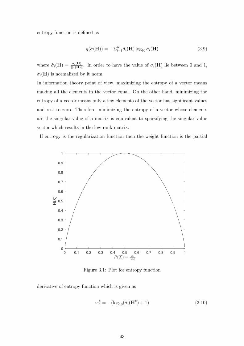
entropy function is defined as
g(σ(H)) = −ΣKi=1σi(H) log10 σi(H) (3.9)
where σi(H) = σi(H)||σ(H)|| . In order to have the value of σi(H) lie between 0 and 1,
σi(H) is normalized by it norm.
In information theory point of view, maximizing the entropy of a vector means
making all the elements in the vector equal. On the other hand, minimizing the
entropy of a vector means only a few elements of the vector has significant values
and rest to zero. Therefore, minimizing the entropy of a vector whose elements
are the singular value of a matrix is equivalent to sparsifying the singular value
vector which results in the low-rank matrix.
If entropy is the regularization function then the weight function is the partial
0 0.1 0.2 0.3 0.4 0.5 0.6 0.7 0.8 0.9 1
P (X) = xi
||xi ||
0
0.1
0.2
0.3
0.4
0.5
0.6
0.7
0.8
0.9
1
H(X
)
Figure 3.1: Plot for entropy function
derivative of entropy function which is given as
wki = −(log10(σi(Hk) + 1) (3.10)
43
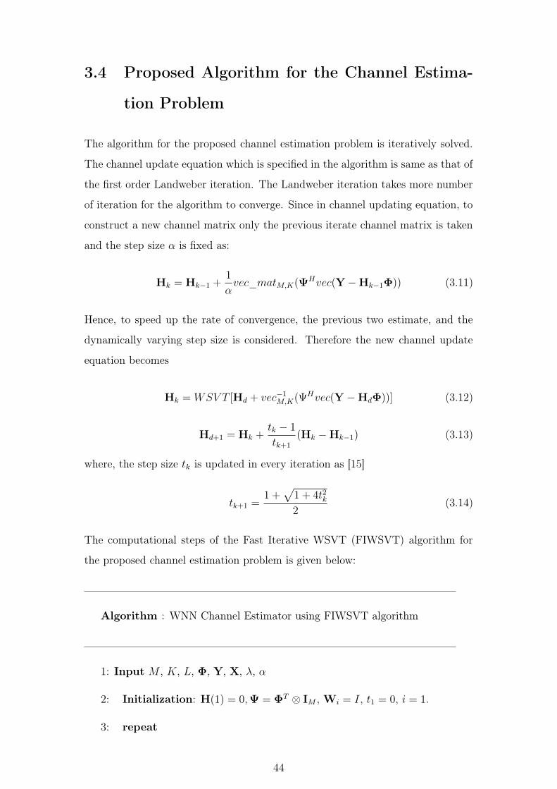
3.4 Proposed Algorithm for the Channel Estima-
tion Problem
The algorithm for the proposed channel estimation problem is iteratively solved.
The channel update equation which is specified in the algorithm is same as that of
the first order Landweber iteration. The Landweber iteration takes more number
of iteration for the algorithm to converge. Since in channel updating equation, to
construct a new channel matrix only the previous iterate channel matrix is taken
and the step size α is fixed as:
Hk = Hk−1 +1
αvec_matM,K(Ψ
Hvec(Y −Hk−1Φ)) (3.11)
Hence, to speed up the rate of convergence, the previous two estimate, and the
dynamically varying step size is considered. Therefore the new channel update
equation becomes
Hk = WSV T [Hd + vec−1M,K(Ψ
Hvec(Y −HdΦ))] (3.12)
Hd+1 = Hk +tk − 1
tk+1
(Hk −Hk−1) (3.13)
where, the step size tk is updated in every iteration as [15]
tk+1 =1 +
�1 + 4t2k2
(3.14)
The computational steps of the Fast Iterative WSVT (FIWSVT) algorithm for
the proposed channel estimation problem is given below:
Algorithm : WNN Channel Estimator using FIWSVT algorithm
1: Input M , K, L, Φ, Y, X, λ, α
2: Initialization: H(1) = 0,Ψ = ΦT ⊗ IM , Wi = I, t1 = 0, i = 1.
3: repeat
44
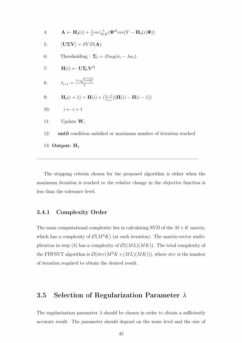
4: A ← Hd(i) +1αvec−1
M,K(ΨHvec(Y −Hd(i)Φ))
5: [UΣV] = SV D(A)
6: Thresholding : Σt = Diag(σi − λwi)
7: H(i) ← UΣtVH
8: ti+1 =1+√
1+4t2i2
9: Hd(i+ 1) = H(i) + ( ti−1ti+1
)(H(i)−H(i− 1))
10: i ← i+ 1
11: Update Wi
12: until condition satisfied or maximum number of iteration reached
13: Output: Hd
The stopping criteria chosen for the proposed algorithm is either when the
maximum iteration is reached or the relative change in the objective function is
less than the tolerance level.
3.4.1 Complexity Order
The main computational complexity lies in calculating SVD of the M×K matrix,
which has a complexity of O(M 2K) (at each iteration). The matrix-vector multi-
plication in step (4) has a complexity of O((ML)(MK)). The total complexity of
the FIWSVT algorithm is O(iter(M 2K+(ML)(MK))), where iter is the number
of iteration required to obtain the desired result.
3.5 Selection of Regularization Parameter λ
The regularization parameter λ should be chosen in order to obtain a sufficiently
accurate result. The parameter should depend on the noise level and the size of
45

the received signal matrix at the BS. To obtain convergence of the cost function,
the regularization parameter should satisfy the condition λ ≥ ||NΦH ||2.
Lemma 1. Consider a matrix A is M ×L random matrix whose entries are in-
dependent random variables with mean zero and variance one. B is an L×K non
random matrix with independent columns and ||B||2 ≤ 1. Then the resultant prod-
uct of the matrix W = AB will have entries random with an independent column.
Therefore, the spectral norm of the matrix W is given as ||W||2 ≈ C(√M +
√K),
where C is constant [60],[61].
Using Lemma 1 the value for the regularization parameter λ is determined.
The training matrix Φ is a K × L deterministic BPSK data at the receiver and
||Φ||2 > 1. In order to use the above results in Lemma 1, Φ can be normalized
by σ1(Φ). N is a random Gaussian matrix with zero mean and σ2n variance then
λ ≥ ||NΦH ||2 ≈ C1σn(√M +
√K) where C1 = C/σ1(Φ).
3.6 Simulation Results and Discussion
In this section, the proposed WNN channel estimator is evaluated using the per-
formance index normalized MSE and Downlink average sum-rate for the non-
orthogonal training sequence. The parameters of the single cell massive MIMO
system for simulation is given in Table.3.1.
Parameters Values
Number of BS Antennas (M) 100
Number of users in a cell (K) 40
Number of scatterers (P ) 10, 15, 20
Length of the training data (L) 50 [62]
Antenna Spacing (D/λ) 0.3
Table 3.1: System Parameters
46
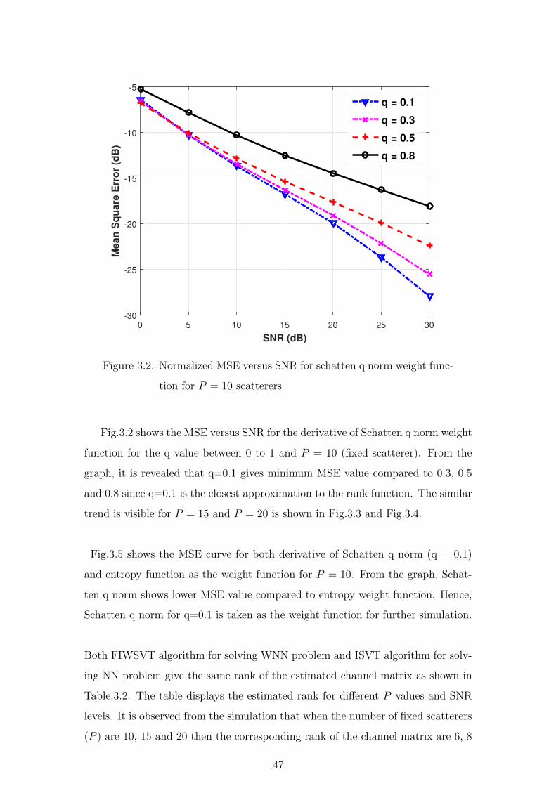
0 5 10 15 20 25 30
SNR (dB)
-30
-25
-20
-15
-10
-5
Me
an
Sq
ua
re E
rro
r (d
B)
q = 0.1
q = 0.3
q = 0.5
q = 0.8
Figure 3.2: Normalized MSE versus SNR for schatten q norm weight func-
tion for P = 10 scatterers
Fig.3.2 shows the MSE versus SNR for the derivative of Schatten q norm weight
function for the q value between 0 to 1 and P = 10 (fixed scatterer). From the
graph, it is revealed that q=0.1 gives minimum MSE value compared to 0.3, 0.5
and 0.8 since q=0.1 is the closest approximation to the rank function. The similar
trend is visible for P = 15 and P = 20 is shown in Fig.3.3 and Fig.3.4.
Fig.3.5 shows the MSE curve for both derivative of Schatten q norm (q = 0.1)
and entropy function as the weight function for P = 10. From the graph, Schat-
ten q norm shows lower MSE value compared to entropy weight function. Hence,
Schatten q norm for q=0.1 is taken as the weight function for further simulation.
Both FIWSVT algorithm for solving WNN problem and ISVT algorithm for solv-
ing NN problem give the same rank of the estimated channel matrix as shown in
Table.3.2. The table displays the estimated rank for different P values and SNR
levels. It is observed from the simulation that when the number of fixed scatterers
(P ) are 10, 15 and 20 then the corresponding rank of the channel matrix are 6, 8
47
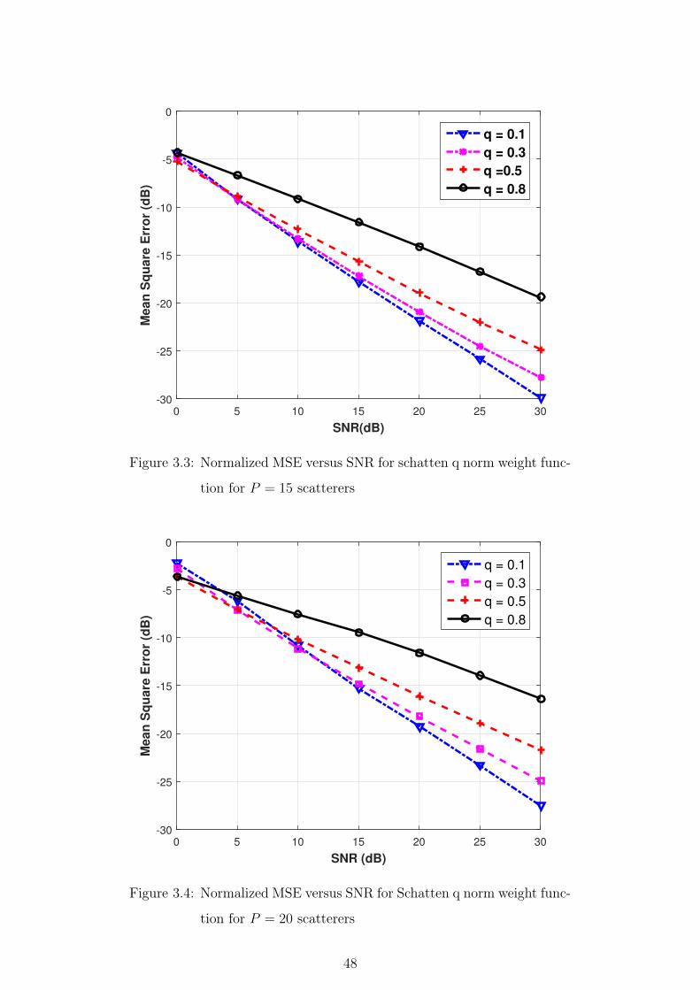
0 5 10 15 20 25 30
SNR(dB)
-30
-25
-20
-15
-10
-5
0
Me
an
Sq
ua
re E
rro
r (d
B)
q = 0.1
q = 0.3
q =0.5
q = 0.8
Figure 3.3: Normalized MSE versus SNR for schatten q norm weight func-
tion for P = 15 scatterers
0 5 10 15 20 25 30
SNR (dB)
-30
-25
-20
-15
-10
-5
0
Me
an
Sq
ua
re E
rro
r (d
B)
q = 0.1
q = 0.3
q = 0.5
q = 0.8
Figure 3.4: Normalized MSE versus SNR for Schatten q norm weight func-
tion for P = 20 scatterers
48
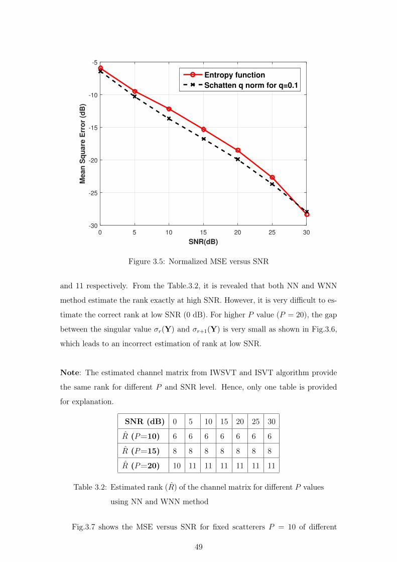
0 5 10 15 20 25 30
SNR(dB)
-30
-25
-20
-15
-10
-5
Me
an
Sq
ua
re E
rro
r (d
B)
Entropy function
Schatten q norm for q=0.1
Figure 3.5: Normalized MSE versus SNR
and 11 respectively. From the Table.3.2, it is revealed that both NN and WNN
method estimate the rank exactly at high SNR. However, it is very difficult to es-
timate the correct rank at low SNR (0 dB). For higher P value (P = 20), the gap
between the singular value σr(Y) and σr+1(Y) is very small as shown in Fig.3.6,
which leads to an incorrect estimation of rank at low SNR.
Note: The estimated channel matrix from IWSVT and ISVT algorithm provide
the same rank for different P and SNR level. Hence, only one table is provided
for explanation.
SNR (dB) 0 5 10 15 20 25 30
R (P=10) 6 6 6 6 6 6 6
R (P=15) 8 8 8 8 8 8 8
R (P=20) 10 11 11 11 11 11 11
Table 3.2: Estimated rank (R) of the channel matrix for different P values
using NN and WNN method
Fig.3.7 shows the MSE versus SNR for fixed scatterers P = 10 of different
49
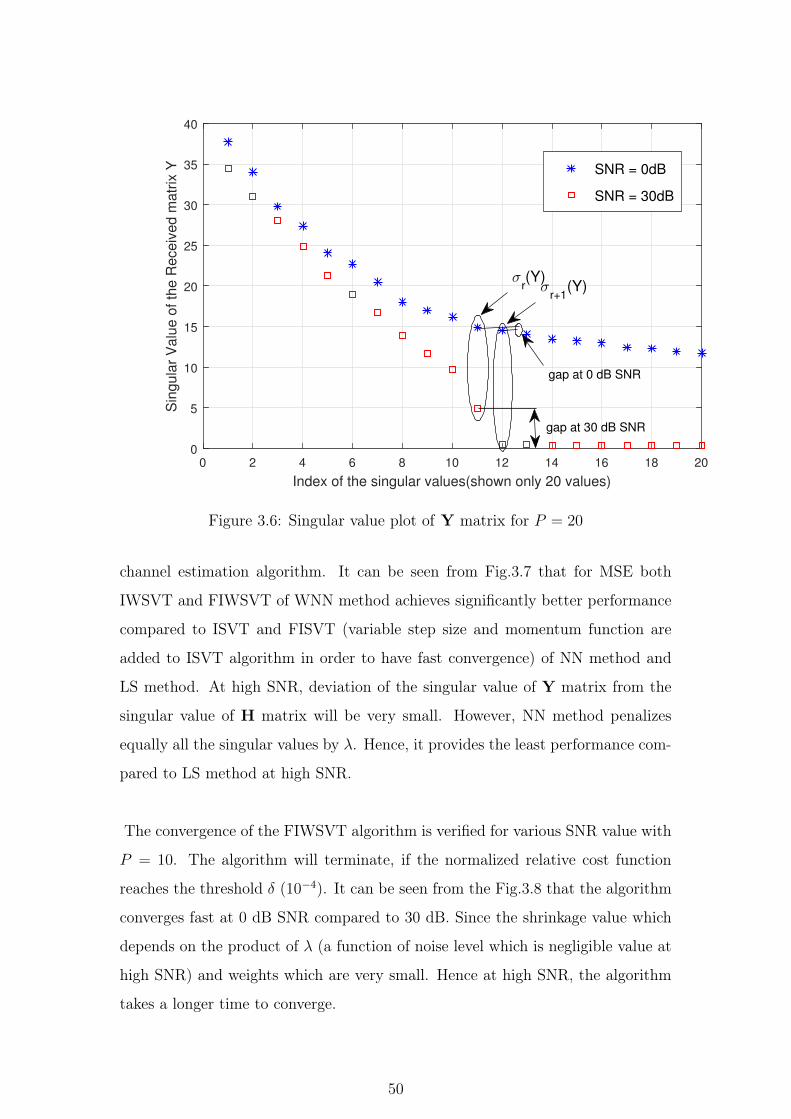
0 2 4 6 8 10 12 14 16 18 20
Index of the singular values(shown only 20 values)
0
5
10
15
20
25
30
35
40
Sin
gu
lar
Va
lue
of
the
Re
ce
ive
d m
atr
ix Y SNR = 0dB
SNR = 30dB
σr(Y)σ
r+1(Y)
gap at 0 dB SNR
gap at 30 dB SNR
Figure 3.6: Singular value plot of Y matrix for P = 20
channel estimation algorithm. It can be seen from Fig.3.7 that for MSE both
IWSVT and FIWSVT of WNN method achieves significantly better performance
compared to ISVT and FISVT (variable step size and momentum function are
added to ISVT algorithm in order to have fast convergence) of NN method and
LS method. At high SNR, deviation of the singular value of Y matrix from the
singular value of H matrix will be very small. However, NN method penalizes
equally all the singular values by λ. Hence, it provides the least performance com-
pared to LS method at high SNR.
The convergence of the FIWSVT algorithm is verified for various SNR value with
P = 10. The algorithm will terminate, if the normalized relative cost function
reaches the threshold δ (10−4). It can be seen from the Fig.3.8 that the algorithm
converges fast at 0 dB SNR compared to 30 dB. Since the shrinkage value which
depends on the product of λ (a function of noise level which is negligible value at
high SNR) and weights which are very small. Hence at high SNR, the algorithm
takes a longer time to converge.
50
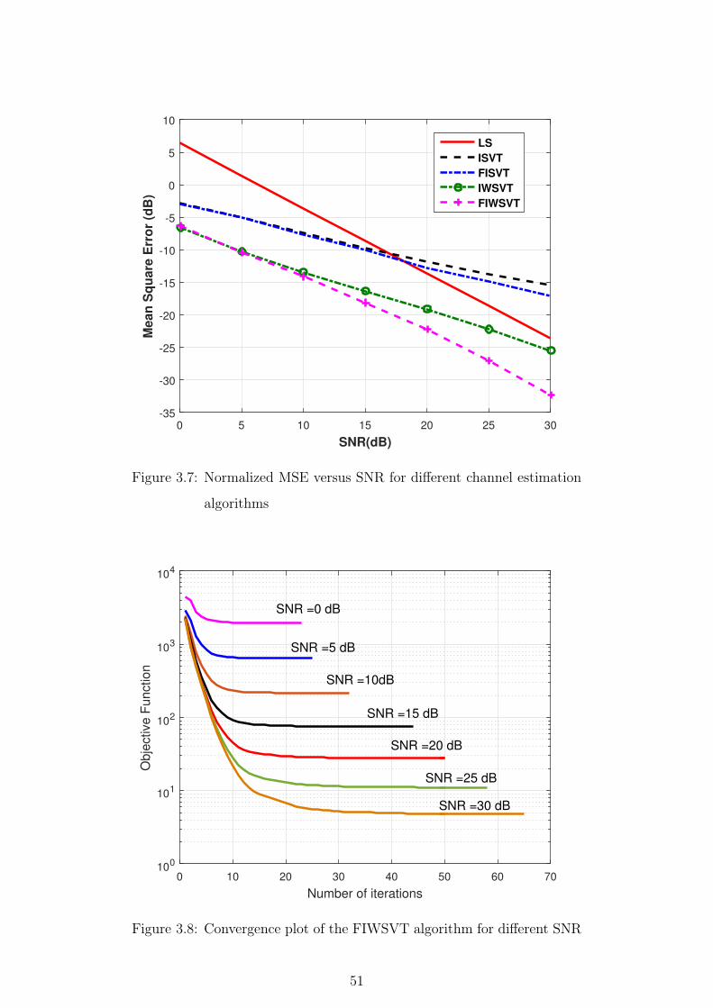
0 5 10 15 20 25 30
SNR(dB)
-35
-30
-25
-20
-15
-10
-5
0
5
10
Me
an
Sq
ua
re E
rro
r (d
B)
LS
ISVT
FISVT
IWSVT
FIWSVT
Figure 3.7: Normalized MSE versus SNR for different channel estimation
algorithms
0 10 20 30 40 50 60 70
Number of iterations
100
101
102
103
104
Ob
jective
Fu
nctio
n
SNR =5 dB
SNR =0 dB
SNR =10dB
SNR =15 dB
SNR =20 dB
SNR =25 dB
SNR =30 dB
Figure 3.8: Convergence plot of the FIWSVT algorithm for different SNR
51
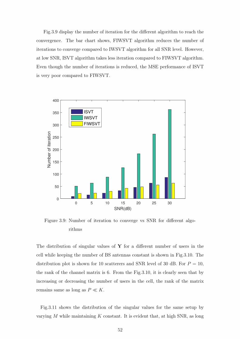
Fig.3.9 display the number of iteration for the different algorithm to reach the
convergence. The bar chart shows, FIWSVT algorithm reduces the number of
iterations to converge compared to IWSVT algorithm for all SNR level. However,
at low SNR, ISVT algorithm takes less iteration compared to FIWSVT algorithm.
Even though the number of iterations is reduced, the MSE performance of ISVT
is very poor compared to FIWSVT.
0 5 10 15 20 25 30
SNR(dB)
0
50
100
150
200
250
300
350
400
Nu
mb
er
of
ite
ratio
n
ISVT
IWSVT
FIWSVT
Figure 3.9: Number of iteration to converge vs SNR for different algo-
rithms
The distribution of singular values of Y for a different number of users in the
cell while keeping the number of BS antennas constant is shown in Fig.3.10. The
distribution plot is shown for 10 scatterers and SNR level of 30 dB. For P = 10,
the rank of the channel matrix is 6. From the Fig.3.10, it is clearly seen that by
increasing or decreasing the number of users in the cell, the rank of the matrix
remains same as long as P � K.
Fig.3.11 shows the distribution of the singular values for the same setup by
varying M while maintaining K constant. It is evident that, at high SNR, as long
52
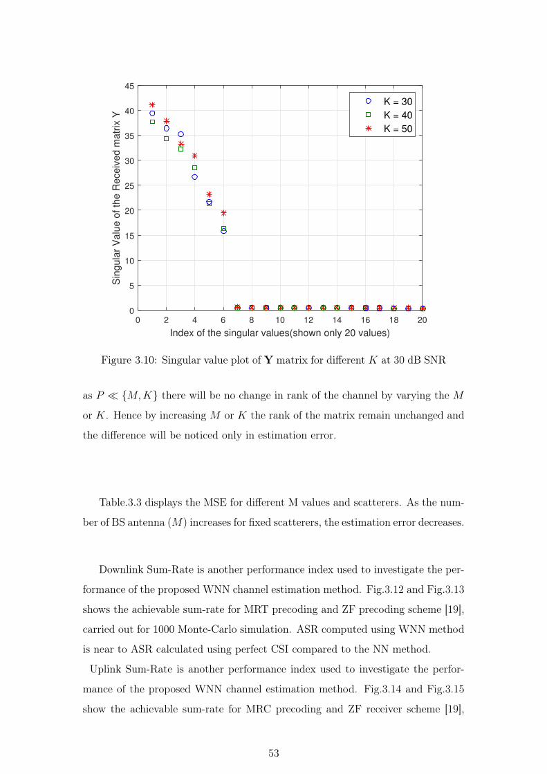
0 2 4 6 8 10 12 14 16 18 20
Index of the singular values(shown only 20 values)
0
5
10
15
20
25
30
35
40
45
Sin
gu
lar
Va
lue
of
the
Re
ce
ive
d m
atr
ix Y
K = 30
K = 40
K = 50
Figure 3.10: Singular value plot of Y matrix for different K at 30 dB SNR
as P � {M,K} there will be no change in rank of the channel by varying the M
or K. Hence by increasing M or K the rank of the matrix remain unchanged and
the difference will be noticed only in estimation error.
Table.3.3 displays the MSE for different M values and scatterers. As the num-
ber of BS antenna (M) increases for fixed scatterers, the estimation error decreases.
Downlink Sum-Rate is another performance index used to investigate the per-
formance of the proposed WNN channel estimation method. Fig.3.12 and Fig.3.13
shows the achievable sum-rate for MRT precoding and ZF precoding scheme [19],
carried out for 1000 Monte-Carlo simulation. ASR computed using WNN method
is near to ASR calculated using perfect CSI compared to the NN method.
Uplink Sum-Rate is another performance index used to investigate the perfor-
mance of the proposed WNN channel estimation method. Fig.3.14 and Fig.3.15
show the achievable sum-rate for MRC precoding and ZF receiver scheme [19],
53

0 2 4 6 8 10 12 14 16 18 20
Index of the singular values(shown only 20 values)
0
5
10
15
20
25
30
35
40
Sin
gu
lar
Va
lue
of
the
Re
ce
ive
d m
atr
ix Y
M = 80
M = 90
M = 100
Figure 3.11: Singular value plot of Y matrix for different M at 30 dB SNR
0 5 10 15 20 25 30
SNR (dB)
0
10
20
30
40
50
60
Achie
vable
Sum
-Rate
(bits/s
/Hz) Perfect CSI
FIWSVT
FIVST
Figure 3.12: Downlink Achievable Sum-Rate versus SNR for different
method (MRT precoder)
54
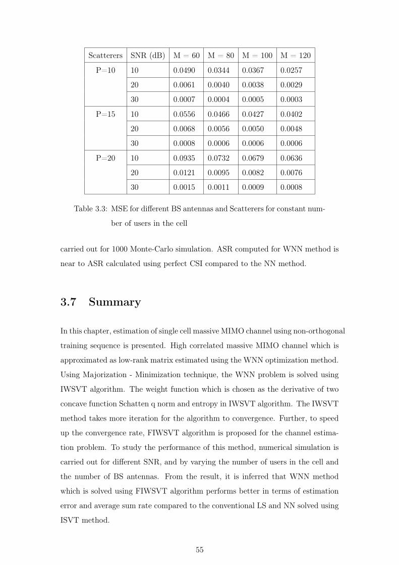
Scatterers SNR (dB) M = 60 M = 80 M = 100 M = 120
P=10 10 0.0490 0.0344 0.0367 0.0257
20 0.0061 0.0040 0.0038 0.0029
30 0.0007 0.0004 0.0005 0.0003
P=15 10 0.0556 0.0466 0.0427 0.0402
20 0.0068 0.0056 0.0050 0.0048
30 0.0008 0.0006 0.0006 0.0006
P=20 10 0.0935 0.0732 0.0679 0.0636
20 0.0121 0.0095 0.0082 0.0076
30 0.0015 0.0011 0.0009 0.0008
Table 3.3: MSE for different BS antennas and Scatterers for constant num-
ber of users in the cell
carried out for 1000 Monte-Carlo simulation. ASR computed for WNN method is
near to ASR calculated using perfect CSI compared to the NN method.
3.7 Summary
In this chapter, estimation of single cell massive MIMO channel using non-orthogonal
training sequence is presented. High correlated massive MIMO channel which is
approximated as low-rank matrix estimated using the WNN optimization method.
Using Majorization - Minimization technique, the WNN problem is solved using
IWSVT algorithm. The weight function which is chosen as the derivative of two
concave function Schatten q norm and entropy in IWSVT algorithm. The IWSVT
method takes more iteration for the algorithm to convergence. Further, to speed
up the convergence rate, FIWSVT algorithm is proposed for the channel estima-
tion problem. To study the performance of this method, numerical simulation is
carried out for different SNR, and by varying the number of users in the cell and
the number of BS antennas. From the result, it is inferred that WNN method
which is solved using FIWSVT algorithm performs better in terms of estimation
error and average sum rate compared to the conventional LS and NN solved using
ISVT method.
55

0 5 10 15 20 25 30
SNR(dB)
0
10
20
30
40
50
60
70
Achie
vable
Sum
-Rate
(bits/s
/Hz)
Perfect CSI
LS
FISVT
FIWSVT
Figure 3.13: Downlink Achievable Sum-Rate versus SNR for different
method (ZF precoder)
0 5 10 15 20 25 30
SNR (dB)
5
10
15
20
25
30
35
40
45
50
55
Ach
ieva
ble
Su
m-R
ate
(bits/s
/Hz)
Perfect CSI
FIWSVT
FIVST
Figure 3.14: Uplink Achievable Sum-Rate versus SNR for different method
( MRC receiver)
56
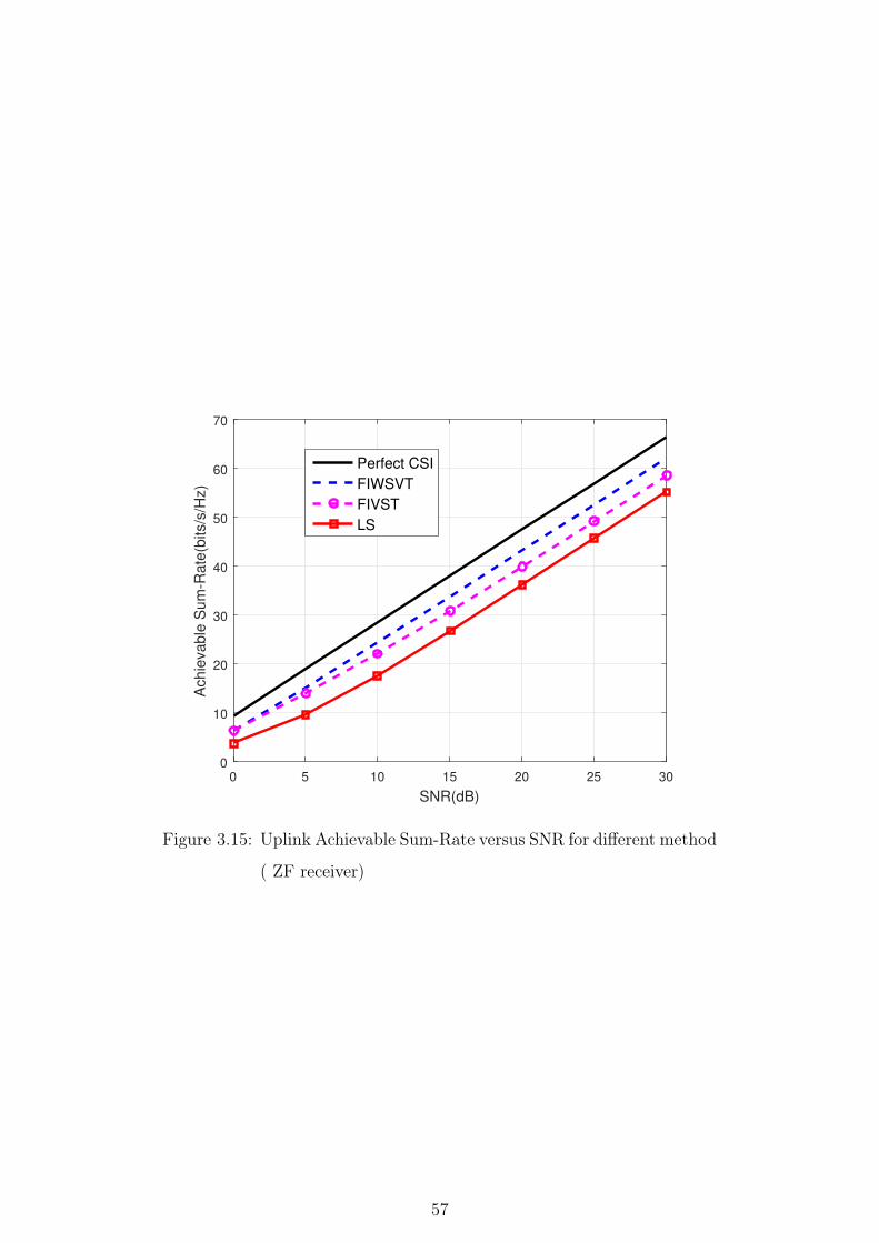
0 5 10 15 20 25 30
SNR(dB)
0
10
20
30
40
50
60
70
Ach
ieva
ble
Su
m-R
ate
(bits/s
/Hz)
Perfect CSI
FIWSVT
FIVST
LS
Figure 3.15: Uplink Achievable Sum-Rate versus SNR for different method
( ZF receiver)
57
CHAPTER 4
Channel Estimation using Orthogonal Pilot
Sequence
4.1 Introduction
The low-rank channel estimation using non-orthogonal training sequence is studied
in chapter 3. To recover the low-rank channel matrix using WNNM method, the
training matrix should satisfy the Restricted Isometric Property (RIP) which is
detailed in Section 4.2. A Partial Random Fourier Matrix (PRFM) satisfying the
RIP is adapted as the training matrix to recover the low-rank channel. In Section
4.3 and 4.4, the reduction in computational complexity of the proposed channel
estimation method using PRFM and the algorithm is discussed.
The proper selection of regularization parameter in order to have the desired
rank for the channel estimation is discussed in Section 4.5. In section 4.6, the
selection of weights in WNNM method in order to satisfy the convexity condition
is outlined. The weights which are proposed for solving WNNM problem is a
function of the regularization parameter, singular values, and tuning parameter.
To achieve minimum MSE for the estimate, the tuning parameters are selected
based on Stein’s unbiased risk estimate which is explained in Section 4.7. The
Mean Square Error (MSE) and Average Sum-Rate (ASR) are the criteria used
to measure the performance of the proposed method and are compared with LS
estimation method and the NNM method for various finite scatterers in different
SNR levels in Section 4.8.
4.2 Selection of Training Matrix
The low rank matrix can be recovered efficiently using Weighted Nuclear Norm
Minimization method, if the training matrix satisfies the Restricted Isometric
Property(RIP) [63]. The RIP condition is stated in Theorem 4.2.1.

Theorem 4.2.1 A matrix Φ satisfies the RIP of order r if there exist a δr ∈ (0, 1)
such that
(1− δr)||H||2F ≤ ||HΦ||2F ≤ (1 + δr)||H||2F (4.1)
which holds for all H with rank(H) ≤ r. This condition implies that, the eigen-
value of the training matrix Φ should lie between [1− δr, 1 + δr].
The matrix satisfies the RIP condition are random Gaussian, random Bernoulli
matrix, and partial random Fourier matrix. In this work, the partial random
Fourier matrix as the training matrix for estimating the channel is adapted which
satisfies near optimal RIP [64]. By choosing this training matrix, the low-rank
channel estimation problem can be solved efficiently.
The design of partial random Fourier matrix is as follows:
1. Select the discrete Fourier matrix F ∈ CL×L with entries Fi,j =1√Lej2π(i−1)(j−1)/L,
i, j ∈ [1, L]
2. Pick the random K row vector out of L from matrix F (L ≥ K)
3. Construct a matrix Φ of size K×L by placing the K row vector of F matrix
in random position.
Remarks: The orthogonality of the design training matrix is preserved even after
the random permutation of row vector [64].
4.3 Convergence Analysis
In this section, convergence analysis for WNN method for the partial DFT training
matrix is discussed. The WNNM cost function is given as
J(h) =1
2||y −Ψh)||22 + λ||H||∗ (4.2)
The convergence of the proposed iterative algorithm is analysed by assuming the
regularizer factor λ = 0. Then the term ||y−Ψh||22 can be solved iteratively using
59
Landweber iterative method [65] in matrix form as
Hi+1 = Hi +1
α(Y − HiΦ)ΦH (4.3)
which can be rewritten as
Hi+1 = Hi(I −1
αΦΦH) +
1
αYΦH (4.4)
Since H0 is initialized to zero matrix, using the above recursion H1 is obtained as
H1 =1
αYΦH (4.5)
and
H2 =1
αYΦH + (I − 1
αΦΦH)YΦH (4.6)
Rearranging the equation H2 in terms of H1
H2 = H1 + (I − 1
αΦΦH)YΦH (4.7)
Similarly, we obtain H3 as
H3 = H2 + (I − 1
αΦΦH)2YΦH (4.8)
In general, the iterative equation is written as
Hi =i−1�
j=0
1
αYΦH(I − 1
αΦΦH)j (4.9)
Using the expression for the sum of a geometric series, we obtain
Hi =1
αYΦH [I − (I − 1
αΦΦH)]−1[I − (I − 1
αΦΦH)i] (4.10)
For a partial DFT matrix ΦΦH = I and if we assume α =1 then (4.10) converges
to YΦH i.e in one iteration.
60

4.4 WNN algorithm for Orthogonal Pilot Sequence
The proposed algorithm for the channel estimation problem is given below:
Algorithm : WNN Channel Estimator
1: Input M,K,L, Φ, Y, λ, α , ν = λ/α
2: A ← YΦH
3: [UΣV] = SV D(A)
4: calculation of weights
5: Thresholding : Sν,w(Σ) = Diag(σi − νwi)
6: Hest ← USν,w(Σ)VH
7: Output: Hest
4.4.1 Complexity Order
The total computational complexity of the IWSVT algorithm for orthogonal train-
ing sequence is O((M 2K + (ML)(MK))).
4.5 Selection of Regularization Parameter λ
The accurate rank estimation of the channel matrix is crucial as the rank of the
Multiuser MIMO matrix determines the number of users data stream can be served
simultaneously by the BS within the same time and frequency bandwidth. The
correct rank estimation improves the channel estimation quality which is very
important in designing the beamforming vector as well as for allocating different
power levels to different users.
61
The regularization parameter λ should be chosen carefully. By choosing larger
value, Hest will become zero and for lesser value introduces more noise to the
estimates. The parameter should depend on the noise level and the size of the
received signal matrix at the BS. To obtain faster convergence of the cost function,
the regularization parameter should satisfy the condition
λ ≥ ||NΦH ||2 (4.11)
When a Gaussian matrix is multiplied by the unitary matrix then the resultant
matrix is Gaussian. Therefore, λ should be greater than or equal to the largest
singular value of the matrix N where N = NΦH .
From the Non-asymptotic theory, the largest singular value of the random
matrices with size M ×K with independent entries (and with zero mean and unit
variance) is√M +
√K. Since the entries of N are independent Gaussian with
zero mean and variance σ2n then,
λ ≥ ||N||2= σn(
√M +
√K)
(4.12)
For simulation, the lower bound value is considered.
4.6 Selection of Weight Function
In general, WNN Minimization problem is a nonconvex optimization problem. For
WNN to be the convex function, the weights must be non-decreasing with respect
to the singular values, which is proved in [11] and [17]. In such a case, the estimated
singular values using WNN method will be in decreasing order resulting in the
same order as the singular value obtained from the NN minimization problem.
Therefore, the condition imposed on weights are 0 ≤ w1 ≤ w2 ≤ · · · ≤ wK and
the estimated singular value is given by the equation
σest = σi − νwi (4.13)
62
So that larger singular values are less penalized to reduce the bias and small
singular values are heavily penalized to induce sparsity and there by a reduction
in the rank of the matrix. To satisfy the increasing condition, the weight is chosen
as an inverse function of the singular value as given below
wi =
�ν
σi
�γ−1
(4.14)
where the tuning parameter γ is chosen as ≥ 1. Since ν is constant then the weight
is a function of singular values. As singular values are arranged in decreasing
order then their corresponding weights will be arranged in increasing order, thus
convexity is achieved. If γ = 1 then the estimated singular value is
σest = σi − ν
�ν
σi
�γ−1
σest = σi − ν
is the solution of NNM problem and is a biased estimator.
If γ = ∞ then
σest =
σi σi ≥ ν
0 σi < ν
and is the hard thresholding of the singular value which contains original singular
values plus noise. Hence, the proper selection of tuning parameter leads to unbi-
ased estimator. Therefore, γ is chosen by minimizing the Stein’s Unbiased Risk
Estimator (SURE) [66] [67] which is a function of γ .
4.7 Stein’s Unbiased Risk Estimator
The tuning parameter γ should be carefully chosen because too much of shrinkage
of the singular value by the threshold parameter νwi results in large bias to the
estimates whereas a little shrinkage results in high variance. Hence γ is selected
by minimizing the mean square error given by
MSE = E||H − Hest(γ)||2F (4.15)
63
where Hest is obtained from nonlinear biased estimator. However, the true mean-
squared error of an estimator is a function of the unknown parameter H to be
estimated, and thus cannot be determined accurately. Therefore, Stein’s unbiased
risk estimate [66],[68] is an unbiased estimator of the mean-squared error of a
nonlinear biased estimator is used to estimate γ, by minimizing the SURE function
with respect to γ.
E(SURE) = MSE. (4.16)
In order to obtain SURE function, the received matrix Y is multiplied by ΦH
YΦH = HΦΦH + NΦH (4.17)
Therefore, the received matrix becomes
Y = H + N (4.18)
where Y = YΦH , N = NΦH and ΦΦH = I.
The estimation of the unknown channel matrix H from the received matrix Y is
given as
Hest = USν,w(Σ)VH (4.19)
where U and V are obtain from SVD of YΦH . The soft thresholding operator
Sν,w which is a function of w discussed in Section 4.6 is given by
Sν,w(σi) = σimax(1− νγ
σγi
, 0) (4.20)
The estimator using the thresholding function is given by
Hest(γ)
min(M,K)�
i=1
Uiσimax(1− νγ
σγi
, 0)VHi (4.21)
ν ≥ 0 and γ ≥ 1. Thus, minimizing SURE can act as a surrogate for minimizing
the MSE. To remove the dependency of the true channel matrix H, a simple
64
manipulation is done in the equation in order to determine optimal γ value.
SURE(γ) = E||H − Hest(γ)||2F= E||H + Y − Y − Hest(γ)||2F= E||H − Y||2F + E||Y − Hest(γ)||2F + 2E((H − Y)T (Y − Hest(γ)))
= −E||N||2F + E||Y − Hest(γ)||2F + 2E((H − Y)T (Y − Hest(γ)))
= −MKσ2n + E||Y − Hest(γ)||2F + 2E((H − Y)T (Y − Hest(γ)))
where div(Hest(γ)) = E((H− Y)T (Y−Hest(γ))) is the divergence of the estimate
Hest(γ) and
E||Y − Hest(γ)||2F =
min(M,K)�
i=1
σ2imin(
ν2γ
σ2γi
, 1) (4.22)
Therefore, SURE formula can be written as
SURE(γ) = −MKσ2n +
min(M,K)�
i=1
σ2imin(
ν2γ
σ2γi
, 1) + 2σ2ndiv(Hest(γ)) (4.23)
Candes et al. in [66] given the closed form of divergence as
div(Hest(γ)) =
min(M,K)�
i=1
(S�ν,w(σi)+|M−K|Sν,w(σi)
σi
)+2
min(M,K)�
t�=i,t=1
σiSν,w(σi)
σ2i − σ2
t
(4.24)
S�ν,w(σi) is the differentiation of Sν,w(σi) with respect to σi and it is given as
S�ν,w(σi) = (1 + (γ − 1)
νγ
σγi
).1(σi > ν)
where
1(σi > ν)
1 ifσi > ν
0 otherwise
Substituting both Sν,w(σi) and S�ν,w(σi) into divergence equation. Then we can
get divergence equation as
65
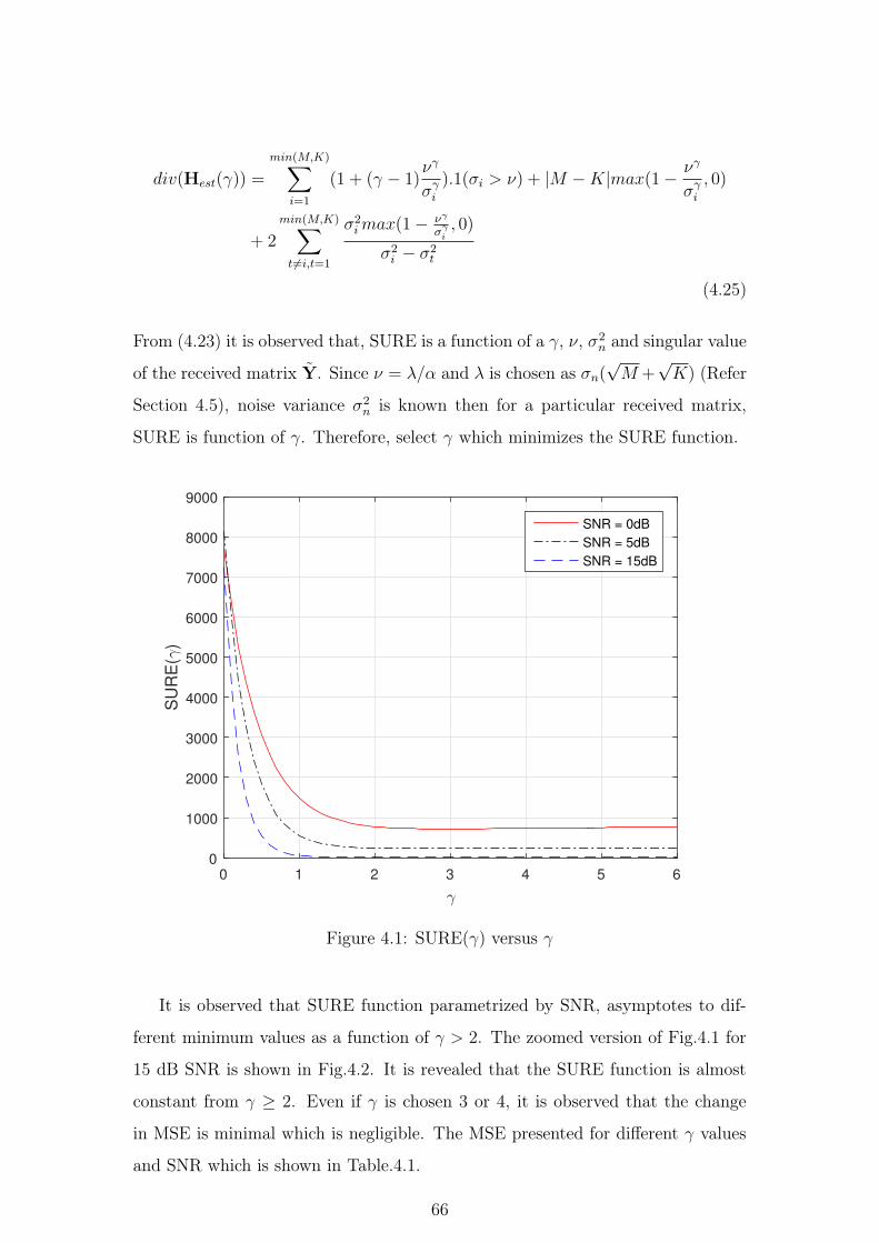
div(Hest(γ)) =
min(M,K)�
i=1
(1 + (γ − 1)νγ
σγi
).1(σi > ν) + |M −K|max(1− νγ
σγi
, 0)
+ 2
min(M,K)�
t�=i,t=1
σ2imax(1− νγ
σγi, 0)
σ2i − σ2
t
(4.25)
From (4.23) it is observed that, SURE is a function of a γ, ν, σ2n and singular value
of the received matrix Y. Since ν = λ/α and λ is chosen as σn(√M +
√K) (Refer
Section 4.5), noise variance σ2n is known then for a particular received matrix,
SURE is function of γ. Therefore, select γ which minimizes the SURE function.
0 1 2 3 4 5 6
γ
0
1000
2000
3000
4000
5000
6000
7000
8000
9000
SU
RE
(γ)
SNR = 0dB
SNR = 5dB
SNR = 15dB
Figure 4.1: SURE(γ) versus γ
It is observed that SURE function parametrized by SNR, asymptotes to dif-
ferent minimum values as a function of γ > 2. The zoomed version of Fig.4.1 for
15 dB SNR is shown in Fig.4.2. It is revealed that the SURE function is almost
constant from γ ≥ 2. Even if γ is chosen 3 or 4, it is observed that the change
in MSE is minimal which is negligible. The MSE presented for different γ values
and SNR which is shown in Table.4.1.
66
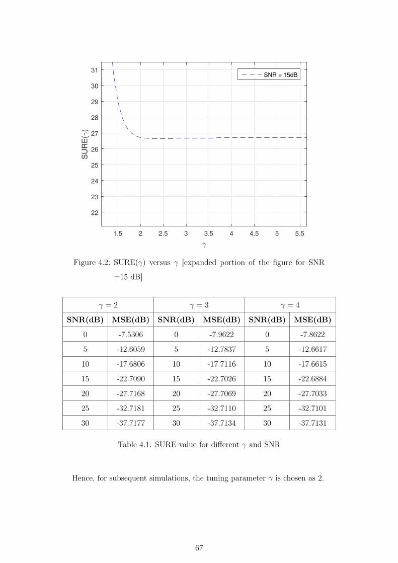
1.5 2 2.5 3 3.5 4 4.5 5 5.5
γ
22
23
24
25
26
27
28
29
30
31
SU
RE
(γ)
SNR = 15dB
Figure 4.2: SURE(γ) versus γ [expanded portion of the figure for SNR
=15 dB]
γ = 2 γ = 3 γ = 4
SNR(dB) MSE(dB) SNR(dB) MSE(dB) SNR(dB) MSE(dB)
0 -7.5306 0 -7.9622 0 -7.8622
5 -12.6059 5 -12.7837 5 -12.6617
10 -17.6806 10 -17.7116 10 -17.6615
15 -22.7090 15 -22.7026 15 -22.6884
20 -27.7168 20 -27.7069 20 -27.7033
25 -32.7181 25 -32.7110 25 -32.7101
30 -37.7177 30 -37.7134 30 -37.7131
Table 4.1: SURE value for different γ and SNR
Hence, for subsequent simulations, the tuning parameter γ is chosen as 2.
67
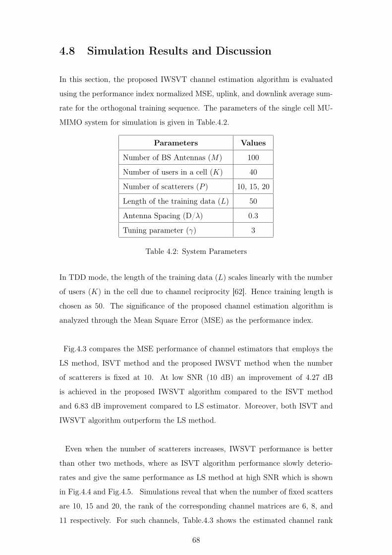
4.8 Simulation Results and Discussion
In this section, the proposed IWSVT channel estimation algorithm is evaluated
using the performance index normalized MSE, uplink, and downlink average sum-
rate for the orthogonal training sequence. The parameters of the single cell MU-
MIMO system for simulation is given in Table.4.2.
Parameters Values
Number of BS Antennas (M) 100
Number of users in a cell (K) 40
Number of scatterers (P ) 10, 15, 20
Length of the training data (L) 50
Antenna Spacing (D/λ) 0.3
Tuning parameter (γ) 3
Table 4.2: System Parameters
In TDD mode, the length of the training data (L) scales linearly with the number
of users (K) in the cell due to channel reciprocity [62]. Hence training length is
chosen as 50. The significance of the proposed channel estimation algorithm is
analyzed through the Mean Square Error (MSE) as the performance index.
Fig.4.3 compares the MSE performance of channel estimators that employs the
LS method, ISVT method and the proposed IWSVT method when the number
of scatterers is fixed at 10. At low SNR (10 dB) an improvement of 4.27 dB
is achieved in the proposed IWSVT algorithm compared to the ISVT method
and 6.83 dB improvement compared to LS estimator. Moreover, both ISVT and
IWSVT algorithm outperform the LS method.
Even when the number of scatterers increases, IWSVT performance is better
than other two methods, where as ISVT algorithm performance slowly deterio-
rates and give the same performance as LS method at high SNR which is shown
in Fig.4.4 and Fig.4.5. Simulations reveal that when the number of fixed scatters
are 10, 15 and 20, the rank of the corresponding channel matrices are 6, 8, and
11 respectively. For such channels, Table.4.3 shows the estimated channel rank
68

0 5 10 15 20 25 30
SNR(dB)
-40
-35
-30
-25
-20
-15
-10
-5
0
Me
an
Sq
ua
re E
rro
r (d
B)
IWSVT
ISVT
LS
Figure 4.3: MSE performance comparison of various channel estimation
schemes for P = 10 scatterers
SNR(dB) Rank(P=10) Rank (P=15) Rank(P=20)
0 6 8 10
5 6 8 11
10 6 8 11
15 6 8 11
20 6 8 11
25 6 8 11
30 6 8 11
Table 4.3: Estimated rank of the channel matrix for different P value
69

0 5 10 15 20 25 30
SNR(dB)
-40
-35
-30
-25
-20
-15
-10
-5
0
Me
an
Sq
ua
re E
rro
r (d
B)
IWSVT
ISVT
LS
Figure 4.4: MSE performance comparison of various channel estimation
schemes for P = 15 scatterers
0 5 10 15 20 25 30
SNR(dB)
-40
-35
-30
-25
-20
-15
-10
-5
0
Me
an
Sq
ua
re E
rro
r (d
B)
IWSVT
ISVT
LS
Figure 4.5: MSE performance comparison of various channel estimation
schemes for P = 20 scatterers
70
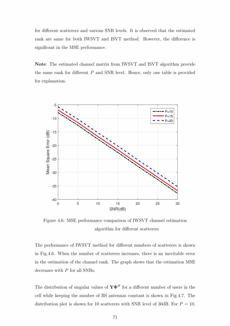
for different scatterers and various SNR levels. It is observed that the estimated
rank are same for both IWSVT and ISVT method. However, the difference is
significant in the MSE performance.
Note: The estimated channel matrix from IWSVT and ISVT algorithm provide
the same rank for different P and SNR level. Hence, only one table is provided
for explanation.
0 5 10 15 20 25 30
SNR(dB)
-40
-35
-30
-25
-20
-15
-10
-5
Me
an
Sq
ua
re E
rro
r (d
B)
P=10
P=15
P=20
Figure 4.6: MSE performance comparison of IWSVT channel estimation
algorithm for different scatterers
The performance of IWSVT method for different numbers of scatterers is shown
in Fig.4.6. When the number of scatterers increases, there is an inevitable error
in the estimation of the channel rank. The graph shows that the estimation MSE
decreases with P for all SNRs.
The distribution of singular values of YΦH for a different number of users in the
cell while keeping the number of BS antennas constant is shown in Fig.4.7. The
distribution plot is shown for 10 scatterers with SNR level of 30dB. For P = 10,
71

0 5 10 15 20
Index of the singular values(shown only 20 values)
0
5
10
15
20
25
30
35
40
Sin
gu
lar
va
lue
s o
f th
e m
atr
ix YΦ
H
K = 30
K = 40
K = 50
Figure 4.7: Singular value plot of YΦH matrix for different K at 30 dB
SNR
the rank of the channel matrix is 6. From Fig.4.7, it is clearly seen that by increas-
ing or decreasing the number of users in the cell, the rank of the matrix remains
same as long as P � K. At high SNR there is a significant gap between the
singular values σr and σr+1. Hence the estimated channel rank will be very close
to as an original rank.
Fig.4.8 also shows the distribution of the singular values for the same setup
by varying K while maintaining M constant. It is evident that, at high SNR,
as long as P � min{M,K}, there will be no change in rank of the channel by
varying the M or K.
It can be observed in Fig.4.8 that at high SNRs, for indices greater than 6, the
singular values collapse to zero implying that for P � M , changing either K or M
does not affect the rank of the channel matrix. However, at low SNRs, as shown
in Fig.4.9 and Fig.4.10, (which are parameterized by M and K respectively) the
singular values are significantly larger than zero for indices greater than 6. In
addition the gap between the singular value at r = 6 and r = 7 decreases, that
72
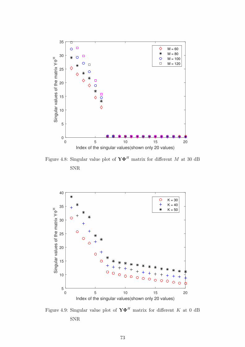
0 5 10 15 20
Index of the singular values(shown only 20 values)
0
5
10
15
20
25
30
35
Sin
gu
lar
va
lue
s o
f th
e m
atr
ix YΦ
H
M = 60
M = 80
M = 100
M = 120
Figure 4.8: Singular value plot of YΦH matrix for different M at 30 dB
SNR
0 5 10 15 20
Index of the singular values(shown only 20 values)
5
10
15
20
25
30
35
40
Sin
gu
lar
va
lue
s o
f th
e m
atr
ix YΦ
H
K = 30
K = 40
K = 50
Figure 4.9: Singular value plot of YΦH matrix for different K at 0 dB
SNR
73
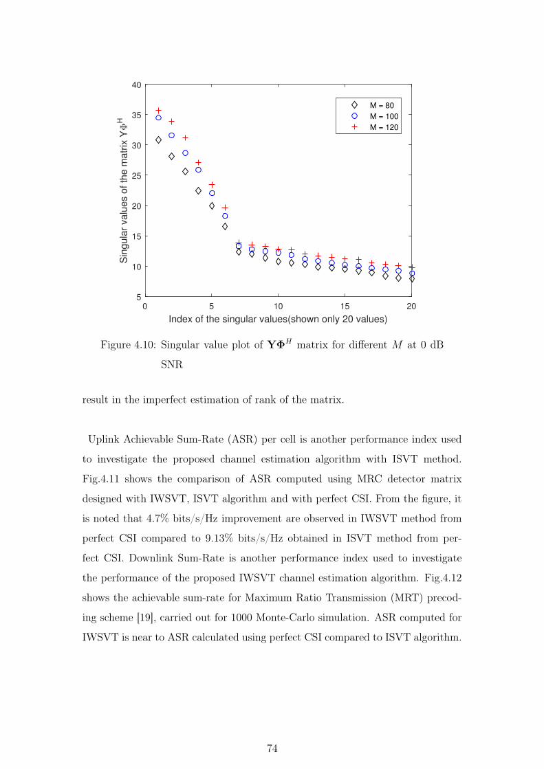
0 5 10 15 20
Index of the singular values(shown only 20 values)
5
10
15
20
25
30
35
40
Sin
gu
lar
va
lue
s o
f th
e m
atr
ix YΦ
H
M = 80
M = 100
M = 120
Figure 4.10: Singular value plot of YΦH matrix for different M at 0 dB
SNR
result in the imperfect estimation of rank of the matrix.
Uplink Achievable Sum-Rate (ASR) per cell is another performance index used
to investigate the proposed channel estimation algorithm with ISVT method.
Fig.4.11 shows the comparison of ASR computed using MRC detector matrix
designed with IWSVT, ISVT algorithm and with perfect CSI. From the figure, it
is noted that 4.7% bits/s/Hz improvement are observed in IWSVT method from
perfect CSI compared to 9.13% bits/s/Hz obtained in ISVT method from per-
fect CSI. Downlink Sum-Rate is another performance index used to investigate
the performance of the proposed IWSVT channel estimation algorithm. Fig.4.12
shows the achievable sum-rate for Maximum Ratio Transmission (MRT) precod-
ing scheme [19], carried out for 1000 Monte-Carlo simulation. ASR computed for
IWSVT is near to ASR calculated using perfect CSI compared to ISVT algorithm.
74
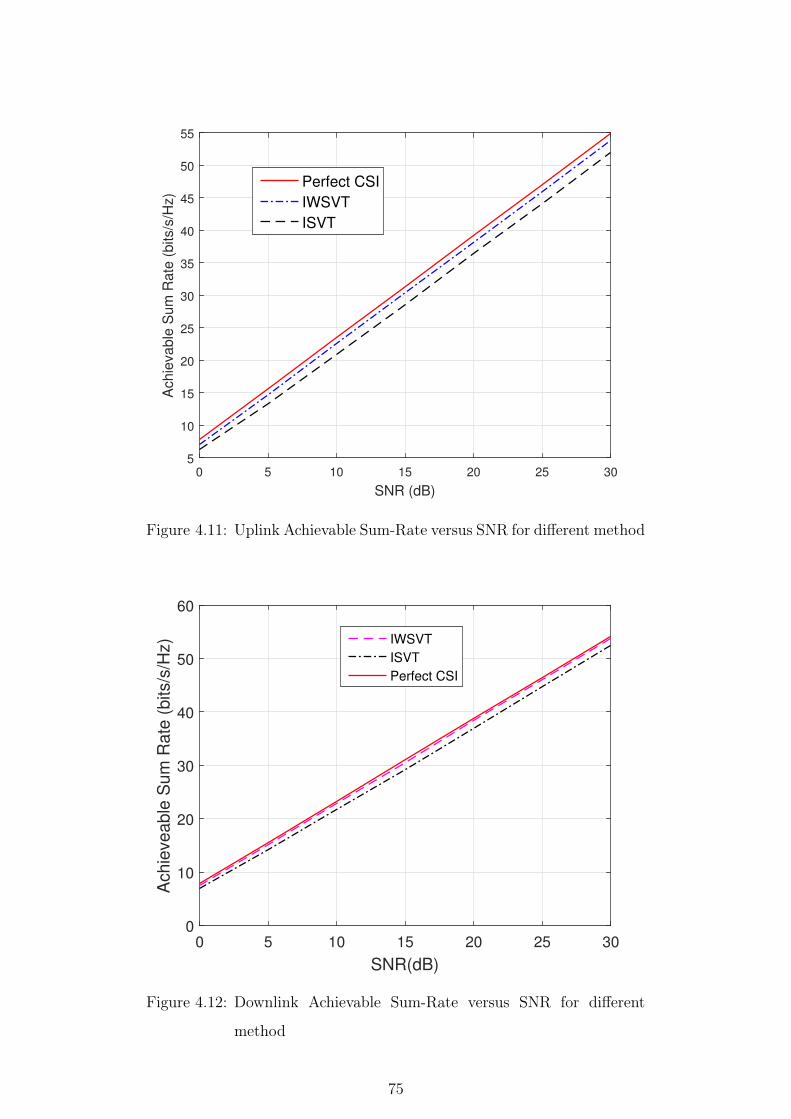
0 5 10 15 20 25 30
SNR (dB)
5
10
15
20
25
30
35
40
45
50
55
Ach
ieva
ble
Su
m R
ate
(b
its/s
/Hz)
Perfect CSI
IWSVT
ISVT
Figure 4.11: Uplink Achievable Sum-Rate versus SNR for different method
0 5 10 15 20 25 30
SNR(dB)
0
10
20
30
40
50
60
Achie
veable
Sum
Rate
(bits/s
/Hz) IWSVT
ISVT
Perfect CSI
Figure 4.12: Downlink Achievable Sum-Rate versus SNR for different
method
75
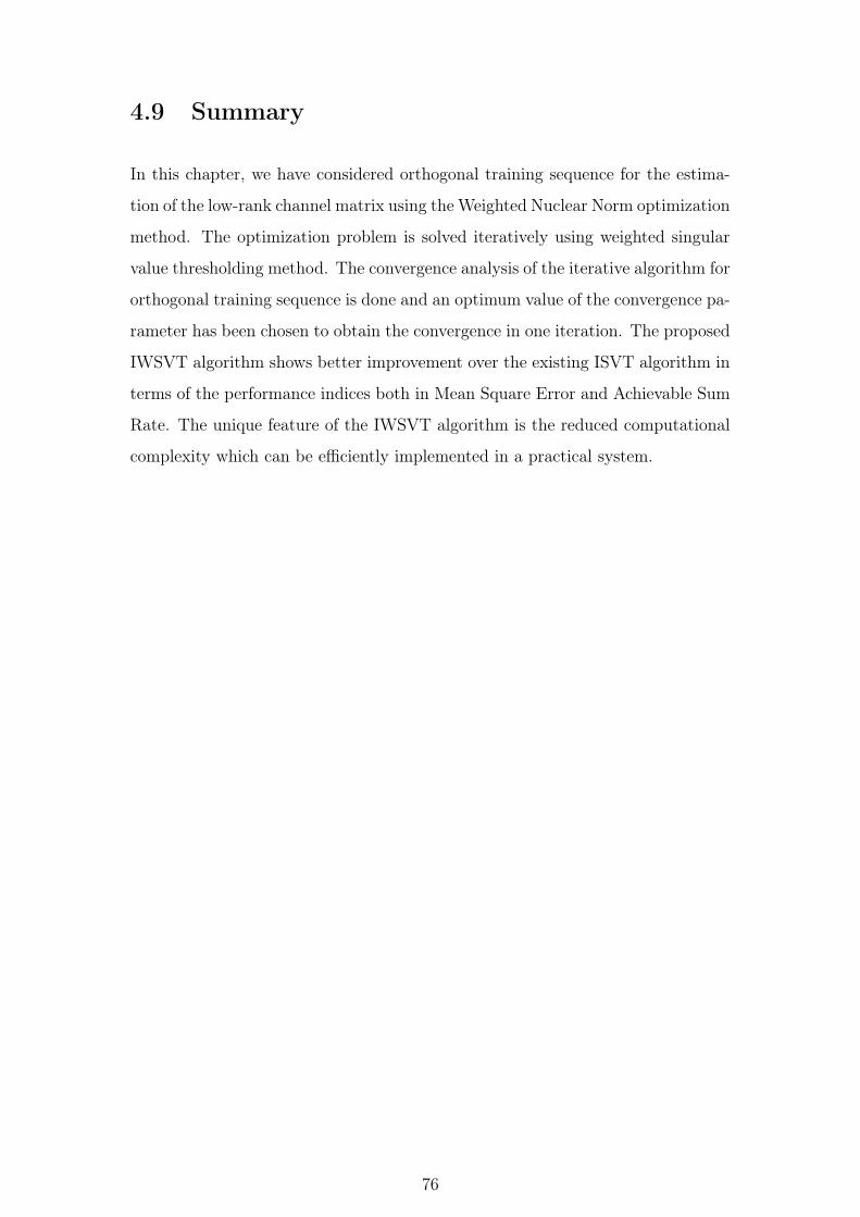
4.9 Summary
In this chapter, we have considered orthogonal training sequence for the estima-
tion of the low-rank channel matrix using the Weighted Nuclear Norm optimization
method. The optimization problem is solved iteratively using weighted singular
value thresholding method. The convergence analysis of the iterative algorithm for
orthogonal training sequence is done and an optimum value of the convergence pa-
rameter has been chosen to obtain the convergence in one iteration. The proposed
IWSVT algorithm shows better improvement over the existing ISVT algorithm in
terms of the performance indices both in Mean Square Error and Achievable Sum
Rate. The unique feature of the IWSVT algorithm is the reduced computational
complexity which can be efficiently implemented in a practical system.
76
CHAPTER 5
Low Rank Channel Estimation in FDD Mode
5.1 Introduction
In TDD mode, CSI acquired in the uplink may not be accurate for the downlink
due to the calibration error of radio frequency chains and limited coherence time.
FDD systems can provide more efficient communications with low latency. In
FDD systems, CSI is obtained at every user by sending the pilot signal from BS
and estimate the channel information with the help of pilot signal. The obtained
CSI is fed back to the BS for precoding the user data.
The number of orthogonal pilots required for downlink channel estimation is
proportional to the number of BS antennas, while the number of orthogonal pilots
required for uplink channel estimation is proportional to the number of scheduled
users. To estimate the downlink channel, the pilot overhead is in the order of
a number of BS antennas which is prohibitively large in Massive MIMO system.
Further, the estimated CSI by the user is feedback to the BS over the uplink chan-
nel. Hence, the overall overhead for uplink is high. Therefore, it is of importance
to explore channel estimation in the downlink than that in the uplink, which can
facilitate massive MIMO to be backward compatible with current FDD dominated
cellular networks. Hence, it is necessary to explore channel estimation method for
massive MIMO based on FDD mode with reduced overhead.
In this chapter, the channel is modeled for downlink and uplink FDD mode
transmission is discussed in Section 5.2. In downlink propagation model, rich
scattering is considered at the user side and most clusters are around BS. All users
in the cell are accessible to cluster at BS leads to same steering matrix which
introduces correlation among the users. Hence, the high dimensional downlink
channel matrix is likely to approximate as low rank, where as in uplink, rich

scattering at user side approximates the channel as high dimensional i.i.d matrix.
The channel estimation method for downlink is carried out at BS is presented in
section 5.3. In Section 5.4, the convergence results for SVP-G, SVP-H, SVP-H
are compared with the proposed WNN method based on the mean square error
at different SNR levels are presented.
5.2 System and Channel Model
Consider the downlink FDD massive MIMO system with M transmit antenna at
BS, serving K single receiver antenna user as shown in Fig.5.1. The BS transmits
Figure 5.1: Single cell downlink transmission
pilot φt ∈ CM×1 at the tth channel use (t = 1, 2, ...L). The received pilot signal at
the kth user is yk ∈ C1×L during L channel use can be expressed as
yk = hkΦ+ nk (5.1)
where Φ = [φ1,φ2, ...φL] is a M × L training matrix constructed from the trans-
mitted pilots during T channel use. nk ∈ C1×L represents the i.i.d additive white
Gaussian noise with elements having zero mean and variance σ2nk
. The channel
78
vector hk ∈ C1×M between the BS and the kth user is given by
hk =P�
p=1
gk,pa(θp) (5.2)
where P is the number of scatterers or number of resolvable physical paths, θp is
the Angle of Departure (AoD) of the pth path. For uniform linear antenna array
the steering vector is defined as
a(θp) = [1, e−j2πDλcos(θp), · · · , e−j2πD
λ(M−1)cos(θp)] (5.3)
where D and λ denote the antenna spacing at the BS and carrier wavelength
respectively.
In channel model, rich scattering is considered at the user side and most clus-
ters are around BS. The clusters that are present around the BS are accessible
to all users introduce correlation among the users, even when the users are geo-
graphically apart. Hence, the channel vectors associated with different users have
the same steering vectors. Thus, the downlink channel matrix is given as
H = GA (5.4)
where G ∈ CK×P is the path gain matrix and A = [a(θ1)T , a(θ2)
T , · · · a(θP )T ] ∈CP×M . Therefore, the rank(H) ≤ min{P,K,M}. Usually, M and K are large
for massive MIMO system and the number of scatterers is assumed relatively
small then the rank(H) ≤ min{P}. Therefore high dimensional downlink channel
matrix is approximated as a low rank channel.
5.3 Downlink Channel Estimation
In conventional FDD system, the channel vector for each user hk (k = 1, 2, · · · , K)
is estimated individually and then the estimated CSI is fed back to the BS. In this
thesis we have assumed, instead of estimating the channel vector at the user side,
the observed pilot signal by each user is fed back to the BS. The joint MIMO
channel estimation of all user is done at the BS. The pilot observation of all user
79

is expressed as
Y = HΦ+N (5.5)
where Y ∈ CK×L, H = [h1T ,h2
T , · · · ,hKT ]T ∈ CK×M is the downlink channel to
be recovered and N = [n1T ,n2
T , · · · ,nKT ]T ∈ CK×L is the downlink noise matrix.
The pilot signal W which is fed back to the BS by all users is given as
W = QY + Z (5.6)
where Q ∈ CM×K is the uplink channel matrix which is modelled as Rayleigh
fading matrix whose entries i.i.d random variable with zero-mean and σ2 variance.
Z ∈ CM×L is the uplink noise matrix whose entries follows CN (0, σ2z).
To recover the downlink channel matrix at BS, firstly Y has to be estimated.
Y matrix is estimated using LS estimation by assuming, uplink channel matrix Q
is known. The estimate Y is given as
Y = (QHQ)−1QHW (5.7)
Further, the estimation of downlink channel matrix at BS can be formulated as a
rank minimization problem:
minH
rank(H) s.t. Y = HΦ (5.8)
This rank minimization problem is nonconvex and NP hard. The above problem
can be reformulated, when rank of the matrix is known as [69]
minH
J(h) = ||y −Ψh||22 s.t. rank(H) ≤ r (5.9)
The solution to the minimization problem is obtained iteratively using Singular
Value Projection (SVP) algorithm. In SVP algorithm, channel matrix can also be
iteratively updated using Newton’s method called SVP-N and the search direction
is ∇2J(h)−1∇J(h). The optimal step size λi is chosen by minimizing the cost
function J .
λiN =min
t{J(hi−1 + t∇2J(h)−1∇J(h))} (5.10)
80
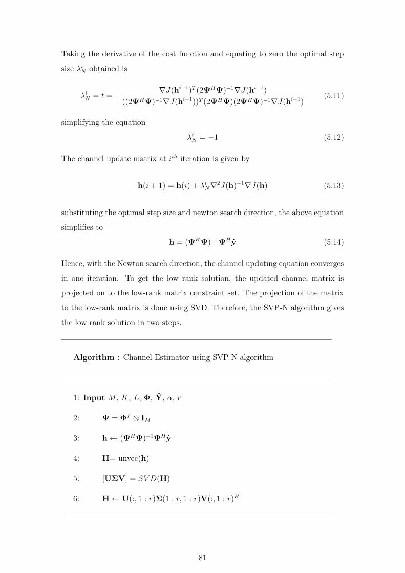
Taking the derivative of the cost function and equating to zero the optimal step
size λiN obtained is
λiN = t = − ∇J(hi−1)T (2ΨHΨ)−1∇J(hi−1)
((2ΨHΨ)−1∇J(hi−1))T (2ΨHΨ)(2ΨHΨ)−1∇J(hi−1)(5.11)
simplifying the equation
λiN = −1 (5.12)
The channel update matrix at ith iteration is given by
h(i+ 1) = h(i) + λiN∇2J(h)−1∇J(h) (5.13)
substituting the optimal step size and newton search direction, the above equation
simplifies to
h = (ΨHΨ)−1ΨH y (5.14)
Hence, with the Newton search direction, the channel updating equation converges
in one iteration. To get the low rank solution, the updated channel matrix is
projected on to the low-rank matrix constraint set. The projection of the matrix
to the low-rank matrix is done using SVD. Therefore, the SVP-N algorithm gives
the low rank solution in two steps.
Algorithm : Channel Estimator using SVP-N algorithm
1: Input M , K, L, Φ, Y, α, r
2: Ψ = ΦT ⊗ IM
3: h ← (ΨHΨ)−1ΨH y
4: H= unvec(h)
5: [UΣV] = SV D(H)
6: H ← U(:, 1 : r)Σ(1 : r, 1 : r)V(:, 1 : r)H
81

Complexity Order: The computational complexity lies in calculation of SVD
of the M × K matrix of rank r is O(M 2r) and matrix-vector multiplication in
step has a complexity of O((ML)(MK)). The total complexity of the SVP-N
algorithm is O(M 2r + (ML)(MK)).
In SVP-N, SVD operation is used only once and hence the error variance will
be more. In SVP algorithm, channel matrix can also be updated using Gradient
decent method (SVP-G) i.e search direction is the gradient of the cost function
∇J(h) = 2ΨH(Ψh− y). The optimal step size λiG is chosen to minimize the cost
function J is given as
λiG =min
t{J(hi−1 + t∇J(hi))} (5.15)
Solving the equation, the optimal step size λiG obtained is
λiG = t = − ∇J(hi−1)T∇J(hi−1)
∇J(hi−1)T (2ΨTΨ)∇J(hi−1)(5.16)
Therefore, the SVP-G algorithm for the channel estimation problem consists of
two steps: (i) channel updating matrix (ii) SVD operation to obtain the low-rank
solution. These two steps solved iteratively are shown below:
Algorithm : Channel Estimator using SVP-G algorithm
1: Input M , K, L, Φ, Y, α, r
2: Initialization: h(1) = 0,Ψ = ΦT ⊗ IM , i = 1.
3: repeat
4: h(i+ 1) ← h(i) + 2λiGΨ
H(Ψh(i)− y)
5: H(i+1)= unvec(h(i+1))
6: [UΣV] = SV D(H(i+ 1))
7: H(i+ 1) ← U(:, 1 : r)Σ(1 : r, 1 : r)V(:, 1 : r)H
82
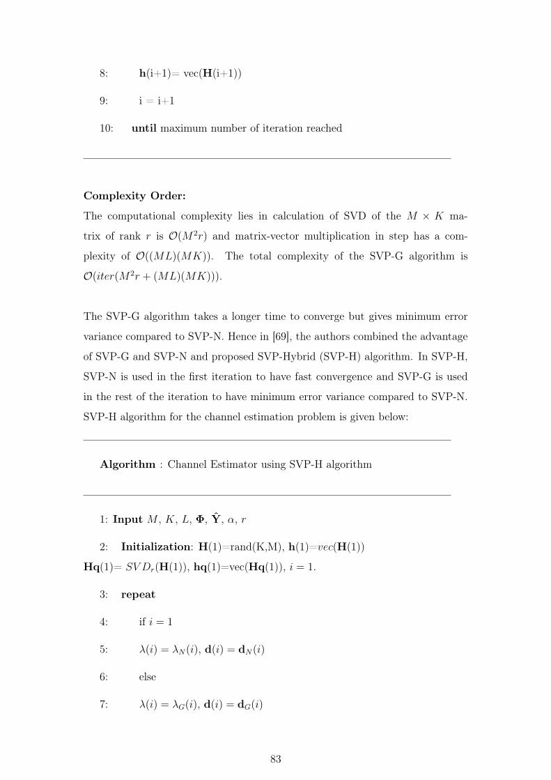
8: h(i+1)= vec(H(i+1))
9: i = i+1
10: until maximum number of iteration reached
Complexity Order:
The computational complexity lies in calculation of SVD of the M × K ma-
trix of rank r is O(M 2r) and matrix-vector multiplication in step has a com-
plexity of O((ML)(MK)). The total complexity of the SVP-G algorithm is
O(iter(M 2r + (ML)(MK))).
The SVP-G algorithm takes a longer time to converge but gives minimum error
variance compared to SVP-N. Hence in [69], the authors combined the advantage
of SVP-G and SVP-N and proposed SVP-Hybrid (SVP-H) algorithm. In SVP-H,
SVP-N is used in the first iteration to have fast convergence and SVP-G is used
in the rest of the iteration to have minimum error variance compared to SVP-N.
SVP-H algorithm for the channel estimation problem is given below:
Algorithm : Channel Estimator using SVP-H algorithm
1: Input M , K, L, Φ, Y, α, r
2: Initialization: H(1)=rand(K,M), h(1)=vec(H(1))
Hq(1)= SV Dr(H(1)), hq(1)=vec(Hq(1)), i = 1.
3: repeat
4: if i = 1
5: λ(i) = λN(i), d(i) = dN(i)
6: else
7: λ(i) = λG(i), d(i) = dG(i)
83
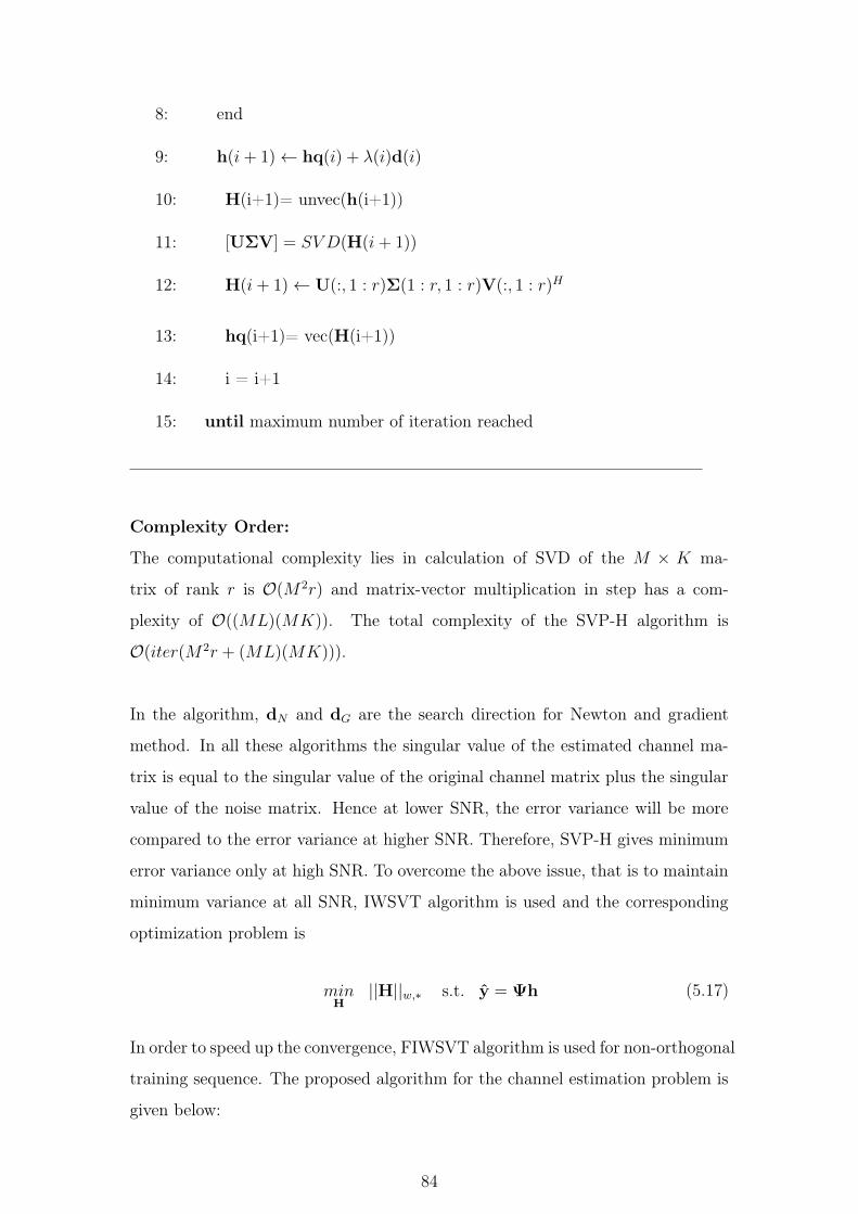
8: end
9: h(i+ 1) ← hq(i) + λ(i)d(i)
10: H(i+1)= unvec(h(i+1))
11: [UΣV] = SV D(H(i+ 1))
12: H(i+ 1) ← U(:, 1 : r)Σ(1 : r, 1 : r)V(:, 1 : r)H
13: hq(i+1)= vec(H(i+1))
14: i = i+1
15: until maximum number of iteration reached
Complexity Order:
The computational complexity lies in calculation of SVD of the M × K ma-
trix of rank r is O(M 2r) and matrix-vector multiplication in step has a com-
plexity of O((ML)(MK)). The total complexity of the SVP-H algorithm is
O(iter(M 2r + (ML)(MK))).
In the algorithm, dN and dG are the search direction for Newton and gradient
method. In all these algorithms the singular value of the estimated channel ma-
trix is equal to the singular value of the original channel matrix plus the singular
value of the noise matrix. Hence at lower SNR, the error variance will be more
compared to the error variance at higher SNR. Therefore, SVP-H gives minimum
error variance only at high SNR. To overcome the above issue, that is to maintain
minimum variance at all SNR, IWSVT algorithm is used and the corresponding
optimization problem is
minH
||H||w,∗ s.t. y = Ψh (5.17)
In order to speed up the convergence, FIWSVT algorithm is used for non-orthogonal
training sequence. The proposed algorithm for the channel estimation problem is
given below:
84

Algorithm : Channel Estimator using FIWSVT algorithm
1: Input M , K, L, Φ, Y, λ, α, r
2: Initialization: Hd(1) = 0,H(1) = 0,Ψ = ΦT ⊗ IM , Wi = I, t1 = 0,
i = 1.
3: repeat
4: A ← Hd(i) + 1αvec−1
M,K(ΨHvec(Y − Hd(i)Φ))
5: [UΣV] = SV D(A)
6: Thresholding : Σt = Diag(σi − λwi)
7: H(i) ← U(:, 1 : r)Σt(1 : r, 1 : r)V(:, 1 : r)H
8: ti+1 =1+√
1+4t2i2
9: Hd(i+ 1) = H(i) + ( ti−1ti+1
)(H(i)− H(i− 1))
10: i ← i+ 1
11: Update Wi
12: until condition satisfied or maximum number of iteration reached
13: Output: Hd
Complexity Order:
The computational complexity lies in calculation of SVD of the M × K ma-
trix of rank r is O(M 2r) and matrix-vector multiplication in step has a com-
plexity of O((ML)(MK)). The total complexity of the FIWSVT algorithm is
O(iter(M 2r + (ML)(MK))).
85
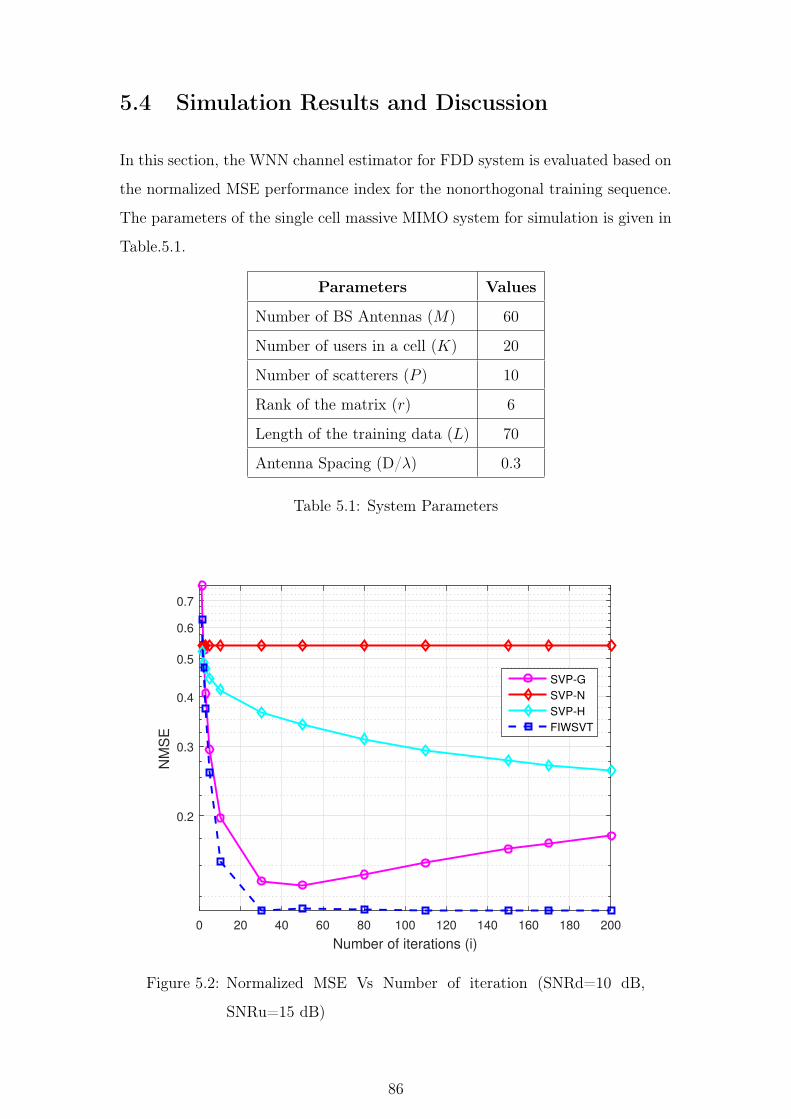
5.4 Simulation Results and Discussion
In this section, the WNN channel estimator for FDD system is evaluated based on
the normalized MSE performance index for the nonorthogonal training sequence.
The parameters of the single cell massive MIMO system for simulation is given in
Table.5.1.
Parameters Values
Number of BS Antennas (M) 60
Number of users in a cell (K) 20
Number of scatterers (P ) 10
Rank of the matrix (r) 6
Length of the training data (L) 70
Antenna Spacing (D/λ) 0.3
Table 5.1: System Parameters
0 20 40 60 80 100 120 140 160 180 200
Number of iterations (i)
0.2
0.3
0.4
0.5
0.6
0.7
NM
SE
SVP-G
SVP-N
SVP-H
FIWSVT
Figure 5.2: Normalized MSE Vs Number of iteration (SNRd=10 dB,
SNRu=15 dB)
86
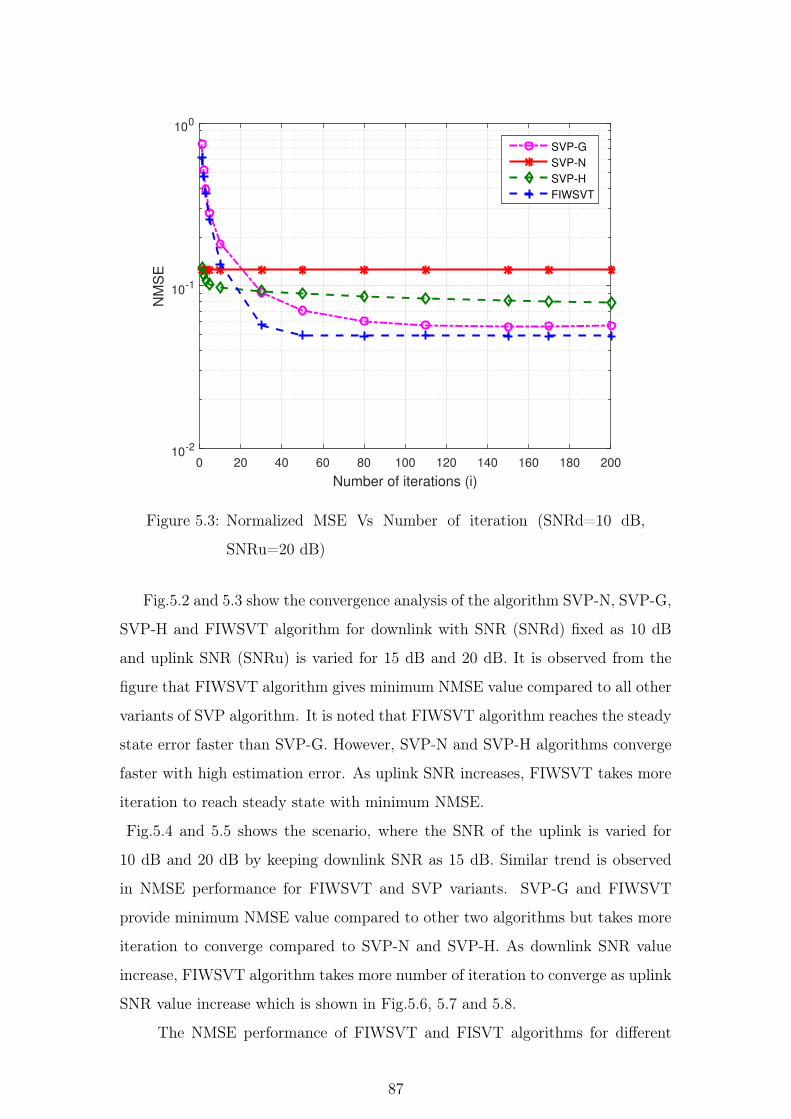
0 20 40 60 80 100 120 140 160 180 200
Number of iterations (i)
10-2
10-1
100
NM
SE
SVP-G
SVP-N
SVP-H
FIWSVT
Figure 5.3: Normalized MSE Vs Number of iteration (SNRd=10 dB,
SNRu=20 dB)
Fig.5.2 and 5.3 show the convergence analysis of the algorithm SVP-N, SVP-G,
SVP-H and FIWSVT algorithm for downlink with SNR (SNRd) fixed as 10 dB
and uplink SNR (SNRu) is varied for 15 dB and 20 dB. It is observed from the
figure that FIWSVT algorithm gives minimum NMSE value compared to all other
variants of SVP algorithm. It is noted that FIWSVT algorithm reaches the steady
state error faster than SVP-G. However, SVP-N and SVP-H algorithms converge
faster with high estimation error. As uplink SNR increases, FIWSVT takes more
iteration to reach steady state with minimum NMSE.
Fig.5.4 and 5.5 shows the scenario, where the SNR of the uplink is varied for
10 dB and 20 dB by keeping downlink SNR as 15 dB. Similar trend is observed
in NMSE performance for FIWSVT and SVP variants. SVP-G and FIWSVT
provide minimum NMSE value compared to other two algorithms but takes more
iteration to converge compared to SVP-N and SVP-H. As downlink SNR value
increase, FIWSVT algorithm takes more number of iteration to converge as uplink
SNR value increase which is shown in Fig.5.6, 5.7 and 5.8.
The NMSE performance of FIWSVT and FISVT algorithms for different
87
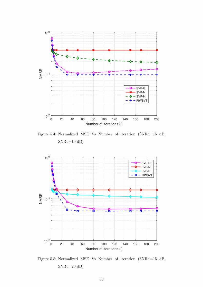
0 20 40 60 80 100 120 140 160 180 200
Number of iterations (i)
10-2
10-1
100
NM
SE
SVP-G
SVP-N
SVP-H
FIWSVT
Figure 5.4: Normalized MSE Vs Number of iteration (SNRd=15 dB,
SNRu=10 dB)
0 20 40 60 80 100 120 140 160 180 200
Number of iterations (i)
10-2
10-1
100
NM
SE
SVP-G
SVP-N
SVP-H
FIWSVT
Figure 5.5: Normalized MSE Vs Number of iteration (SNRd=15 dB,
SNRu=20 dB)
88
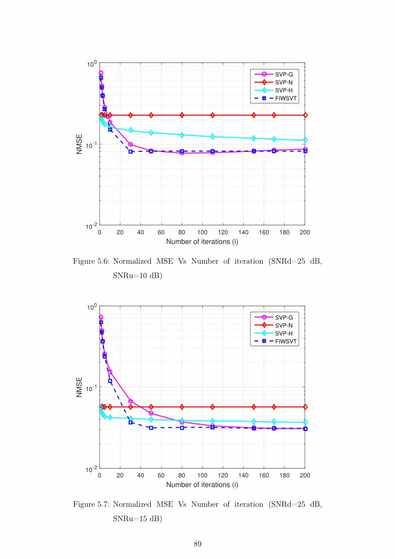
0 20 40 60 80 100 120 140 160 180 200
Number of iterations (i)
10-2
10-1
100
NM
SE
SVP-G
SVP-N
SVP-H
FIWSVT
Figure 5.6: Normalized MSE Vs Number of iteration (SNRd=25 dB,
SNRu=10 dB)
0 20 40 60 80 100 120 140 160 180 200
Number of iterations (i)
10-2
10-1
100
NM
SE
SVP-G
SVP-N
SVP-H
FIWSVT
Figure 5.7: Normalized MSE Vs Number of iteration (SNRd=25 dB,
SNRu=15 dB)
89
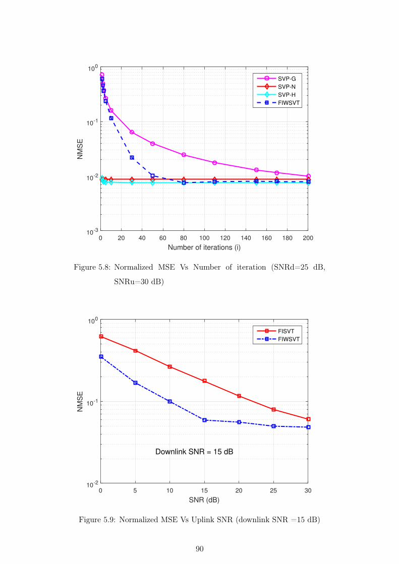
0 20 40 60 80 100 120 140 160 180 200
Number of iterations (i)
10-3
10-2
10-1
100
NM
SE
SVP-G
SVP-N
SVP-H
FIWSVT
Figure 5.8: Normalized MSE Vs Number of iteration (SNRd=25 dB,
SNRu=30 dB)
0 5 10 15 20 25 30
SNR (dB)
10-2
10-1
100
NM
SE
FISVT
FIWSVT
Downlink SNR = 15 dB
Figure 5.9: Normalized MSE Vs Uplink SNR (downlink SNR =15 dB)
90
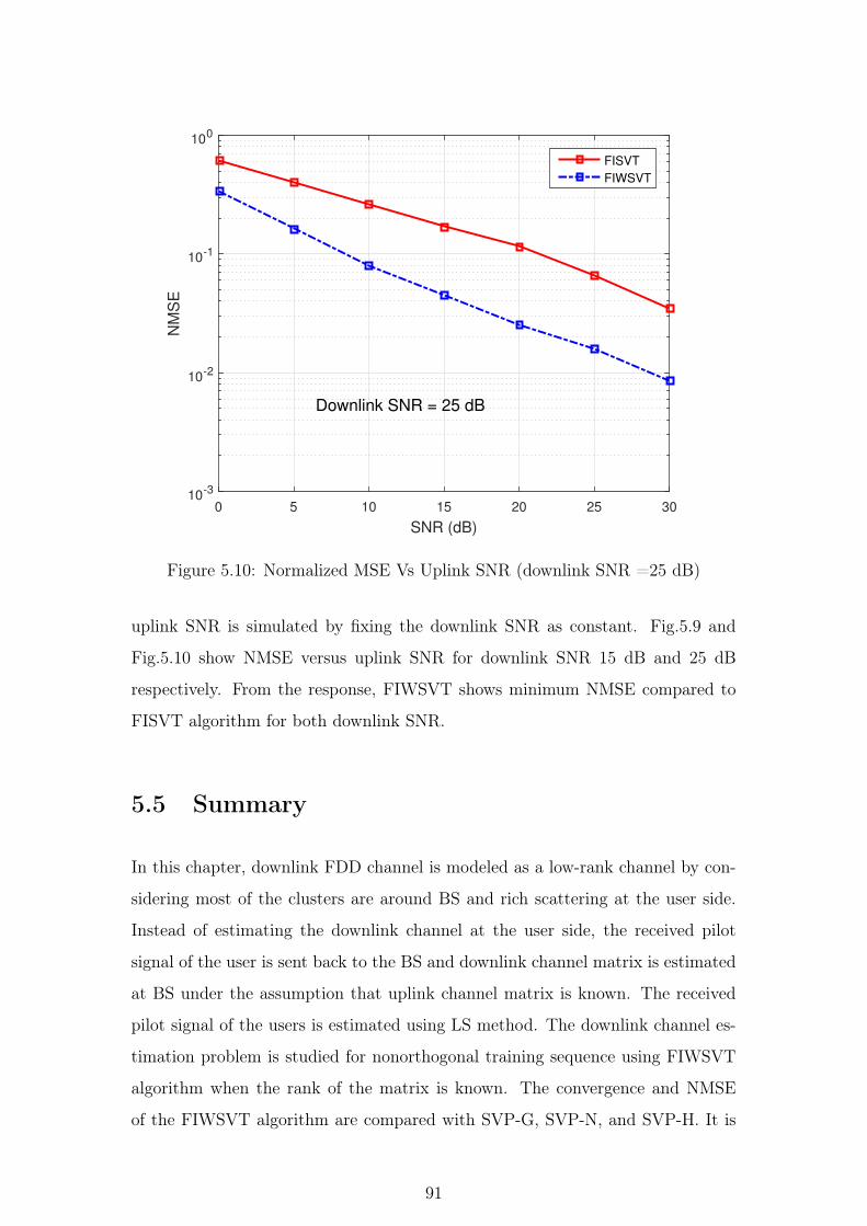
0 5 10 15 20 25 30
SNR (dB)
10-3
10-2
10-1
100
NM
SE
FISVT
FIWSVT
Downlink SNR = 25 dB
Figure 5.10: Normalized MSE Vs Uplink SNR (downlink SNR =25 dB)
uplink SNR is simulated by fixing the downlink SNR as constant. Fig.5.9 and
Fig.5.10 show NMSE versus uplink SNR for downlink SNR 15 dB and 25 dB
respectively. From the response, FIWSVT shows minimum NMSE compared to
FISVT algorithm for both downlink SNR.
5.5 Summary
In this chapter, downlink FDD channel is modeled as a low-rank channel by con-
sidering most of the clusters are around BS and rich scattering at the user side.
Instead of estimating the downlink channel at the user side, the received pilot
signal of the user is sent back to the BS and downlink channel matrix is estimated
at BS under the assumption that uplink channel matrix is known. The received
pilot signal of the users is estimated using LS method. The downlink channel es-
timation problem is studied for nonorthogonal training sequence using FIWSVT
algorithm when the rank of the matrix is known. The convergence and NMSE
of the FIWSVT algorithm are compared with SVP-G, SVP-N, and SVP-H. It is
91

shown through simulation, FIWSVT algorithm has minimum NMSE and faster
convergence at low SNR compared to other algorithms whereas, at high SNR,
it shows minimum NMSE same as SVP-H but with more number of iteration
compared to SVP-H.
92
CHAPTER 6
Conclusion and Future Scope
6.1 Conclusion
The focus of this work was to estimate the finite scattering propagation envi-
ronment for the uplink TDD mode channel. In finite scattering scenario, it was
assumed that the number of scatterers was less than the number of BS antenna
and users. Also, the scatterers were fixed and all users signals were reflected
by the same scatterers. Then their corresponding AoAs for all users were same.
Hence, the correlation among the channel vectors increases which leads to the high
dimensional MIMO channel likely to have the low-rank channel.
The conventional way of estimating the channel was by sending the training
sequences. The LS method estimated the channel matrix without imposing the
low-rank property to the estimated. Hence, the channel estimation problem was
formulated as the rank estimation problem. Since the rank estimation problem
was the nonconvex problem and NP hard to solve, it was formulated as the convex
NNM problem and solved using MM technique. By successive minimization of the
majorizing surrogate function for the given cost function, channel matrix was
estimated iteratively using ISVT algorithm. The main drawback of the ISVT was
penalization of all singular values equally and hence the major information of the
channel matrix associated with the larger singular values was perturbed.
To overcome the drawbacks, WNNM method was proposed in which weight
function includes the prior knowledge of the singular value. By choosing the
weights in an ascending order, the nonconvex problem could be approximated to
the convex optimization problem. The WNNM problem was solved using MM
technique and the corresponding algorithm was IWSVT.
To recover low-rank channel, the proposed algorithm was studied for both or-
thogonal training sequence PRFTM and non-orthogonal training sequence BPSK
modulated data. Using PRFTM, it was proved that the iterative algorithm con-
verges in one iteration and the weights were chosen by minimizing the SURE
unbiased estimator in order to obtain unbiased estimation. The performance of
the algorithm was measured in terms of NMSE, uplink, and downlink average
sum-rate. It was observed that both ISVT and IWSVT algorithm provided same
rank estimation for all SNR level, however, the difference is significant in NMSE
performance (i.e) IWSVT algorithm provide minimum NMSE compared to ISVT
algorithm. The accuracy of the rank estimation algorithm was tested by varying
the number of base station and users in the cell. It was proved through simulation,
as long as the number of scatterers was less in comparison with the number of base
station antenna and user, the exact rank could be estimated.
Non-orthogonal BPSK modulated data was also used to study the performance
of the ISVT and IWSVT algorithm. For non-orthogonal training sequence, itera-
tive algorithm required more iteration to converge. To speed up the convergence
FIWSVT algorithm was proposed for WNNM problem and FISVT algorithm for
NNM problem. Nonconvex weight function was chosen to minimize the mean
square estimation error. Using super gradient property of a concave function,
any nonconvex regularizer function which satisfied smooth property would be con-
verted into weighted nuclear norm problem. The weights for WNNM problem were
chosen as the gradient of the nonconvex regularizer. The algorithm was tested for
Schatten- q norm and entropy function as the two nonconvex regularizer function.
It was shown through simulation that Schatten-q norm regularizer provided min-
imum channel estimation error compared to entropy regularizer. However, both
the regularizer function gave the same rank estimation for all SNR levels. Simi-
larly, the performance of the algorithm was tested by varying the number of BS,
users in the cell and number of fixed scatterers. The results were compared with
the existing LS method, FISVT, and FIWSVT algorithms.
Further, the low-rank channel estimation work was carried out for FDD system,
to show that the proposed method could be applicable to both FDD and TDD
system. In FDD system, downlink channel was assumed to be low rank and uplink
channel as full rank and the estimation of both the channel was done at BS, in
order to reduce the computational burden at the user side. The performance of
the algorithm in FDD system was tested by assuming the rank of the downlink
94
channel is known. The convergence rate and the NMSE versus SNR level results
were compared with SVP-G, SVP-N and SVP-H algorithm when the rank of the
matrix was known.
6.2 Scope for Future Work
This thesis has dealt with channel estimation for single cell Massive MIMO system
with no interference from other cells. However, it is necessary to estimate the
channel of a single cell, when the signal from other cells interferes with the signal
of the desired cell. Consider the case, where BS estimate not only the channel
parameters of desired links in a given cell but also, those of the interference links
from adjacent cells. In multi-cell case, it is necessary to study the interference links,
in order to have interference coordination. In such scenarios, BS has to collect
information regarding CSI of both the desired links within the cell and interference
links from its neighboring cells. Under undesirable finite scattering scenario, the
combined channel matrix can be modeled as low-rank matrix. Therefore, the
analysis presented in this work can be extended to a multi-cell scenario.
For non-orthogonal training sequence, presented in this thesis, the algorithm
takes more iteration to converge. In order to speed up the convergence, variable
step size and previous two estimates are included to find the new estimates. How-
ever, this fast algorithm converges faster at low SNR and take more iteration to
converge at high SNR compared to lower SNR. Hence, the existing algorithm can
be improved to provide a minimum number of iteration for convergence, in high
SNR.
In FDD Massive MIMO system, downlink channel is estimated by keeping
the constraint, rank is known. The analysis in FDD system can be extended
for unknown rank also. The number of training sequence used to estimate the
downlink channel is more than the number of BS antenna. Hence, research can
be made to reduce the number of the pilot sequence.
The channel estimation problem discussed in this thesis is for single cell Massive
MIMO system only. The same channel estimation problem can be extended to
multi-cell scenario also. The pilot contamination is one of the issue in multi-
95

cell massive MIMO system and is mainly caused by non-orthogonality of pilot
sequences used in adjacent cells. In this case, the estimated channel vector in
any cell is the summation of all the channel vectors of users from the neighboring
cells. As the number of interfering cells increase, the problem exponentially grows
and eventually causes system malfunction. Different methods are suggested in
the literature to solve this problem for non cooperative cellular network. These
methods can be extended further to low rank massive MIMO scenario, which can
be made as a future research work.
96
REFERENCES
[1] C. R. Berger, Z. Wang, J. Huang, and S. Zhou, “Application of compres-
sive sensing to sparse channel estimation,” IEEE Communications Magazine,
vol. 48, no. 11, 2010.
[2] D. Gesbert, M. Kountouris, R. W. Heath Jr, C.-B. Chae, and T. Salzer, “Shift-
ing the mimo paradigm,” IEEE signal processing magazine, vol. 24, no. 5, pp.
36–46, 2007.
[3] F. Rusek, D. Persson, B. K. Lau, E. G. Larsson, T. L. Marzetta, O. Edfors,
and F. Tufvesson, “Scaling up mimo: Opportunities and challenges with very
large arrays,” IEEE Signal Processing Magazine, vol. 30, no. 1, pp. 40–60,
2013.
[4] L. Lu, G. Y. Li, A. L. Swindlehurst, A. Ashikhmin, and R. Zhang, “An
overview of massive mimo: Benefits and challenges,” IEEE Journal of Selected
Topics in Signal Processing, vol. 8, no. 5, pp. 742–758, 2014.
[5] H. Q. Ngo, E. G. Larsson, and T. L. Marzetta, “Energy and spectral efficiency
of very large multiuser mimo systems,” IEEE Transactions on Communica-
tions, vol. 61, no. 4, pp. 1436–1449, 2013.
[6] T. L. Marzetta, “Noncooperative cellular wireless with unlimited numbers
of base station antennas,” IEEE Transactions on Wireless Communications,
vol. 9, no. 11, pp. 3590–3600, 2010.
[7] E. G. Larsson, O. Edfors, F. Tufvesson, and T. L. Marzetta, “Massive
mimo for next generation wireless systems,” IEEE Communications Maga-
zine, vol. 52, no. 2, pp. 186–195, 2014.
[8] S. Biswas, C. Masouros, and T. Ratnarajah, “Performance analysis of large
multiuser mimo systems with space-constrained 2-d antenna arrays,” IEEE
Transactions on Wireless Communications, vol. 15, no. 5, pp. 3492–3505,
2016.
97
[9] C. Masouros, M. Sellathurai, and T. Ratnarajah, “Large-scale mimo trans-
mitters in fixed physical spaces: The effect of transmit correlation and mutual
coupling,” IEEE Transactions on Communications, vol. 61, no. 7, pp. 2794–
2804, 2013.
[10] O. Elijah, C. Y. Leow, T. A. Rahman, S. Nunoo, and S. Z. Iliya, “A compre-
hensive survey of pilot contamination in massive mimoâĂŤ5g system,” IEEE
Communications Surveys & Tutorials, vol. 18, no. 2, pp. 905–923, 2016.
[11] D. Neumann, A. Gruendinger, M. Joham, and W. Utschick, “Pilot coordina-
tion for large-scale multi-cell tdd systems,” in Smart Antennas (WSA), 2014
18th International ITG Workshop on. VDE, 2014, pp. 1–6.
[12] V. Saxena, G. Fodor, and E. Karipidis, “Mitigating pilot contamination by
pilot reuse and power control schemes for massive mimo systems,” in Vehicular
Technology Conference (VTC Spring), 2015 IEEE 81st. IEEE, 2015, pp. 1–6.
[13] J. Jose, A. Ashikhmin, T. L. Marzetta, and S. Vishwanath, “Pilot contamina-
tion and precoding in multi-cell tdd systems,” IEEE Transactions on Wireless
Communications, vol. 10, no. 8, pp. 2640–2651, 2011.
[14] F. A. de Figueiredo, F. S. Mathilde, F. P. Santos, F. A. Cardoso, and
G. Fraidenraich, “On channel estimation for massive mimo with pilot contam-
ination and multipath fading channels,” in Communications (LATINCOM),
2016 8th IEEE Latin-American Conference on. IEEE, 2016, pp. 1–4.
[15] H. Yin, D. Gesbert, M. Filippou, and Y. Liu, “A coordinated approach to
channel estimation in large-scale multiple-antenna systems,” IEEE Journal
on Selected Areas in Communications, vol. 31, no. 2, pp. 264–273, 2013.
[16] N. Shariati, E. Bjornson, M. Bengtsson, and M. Debbah, “Low-complexity
polynomial channel estimation in large-scale mimo with arbitrary statistics,”
IEEE Journal of Selected Topics in Signal Processing, vol. 8, no. 5, pp. 815–
830, 2014.
[17] J. Ma and L. Ping, “Data-aided channel estimation in large antenna systems,”
in 2014 IEEE International Conference on Communications (ICC). IEEE,
2014, pp. 4626–4631.
98
[18] H. Q. Ngo and E. G. Larsson, “Evd-based channel estimation in multicell
multiuser mimo systems with very large antenna arrays,” in 2012 IEEE In-
ternational Conference on Acoustics, Speech and Signal Processing (ICASSP).
IEEE, 2012, pp. 3249–3252.
[19] C. Qi and L. Wu, “Uplink channel estimation for massive mimo systems ex-
ploring joint channel sparsity,” Electronics Letters, vol. 50, no. 23, pp. 1770–
1772, 2014.
[20] Y. Nan, L. Zhang, and X. Sun, “Weighted compressive sensing based uplink
channel estimation for time division duplex massive multi-input multi-output
systems,” IET Communications, vol. 11, no. 3, pp. 355–361, 2017.
[21] C. Qi, Y. Huang, S. Jin, and L. Wu, “Sparse channel estimation based on
compressed sensing for massive mimo systems,” in Communications (ICC),
2015 IEEE International Conference on. IEEE, 2015, pp. 4558–4563.
[22] R. G. Baraniuk, “Compressive sensing [lecture notes],” IEEE signal processing
magazine, vol. 24, no. 4, pp. 118–121, 2007.
[23] B. Recht, M. Fazel, and P. A. Parrilo, “Guaranteed minimum-rank solutions
of linear matrix equations via nuclear norm minimization,” SIAM review,
vol. 52, no. 3, pp. 471–501, 2010.
[24] Y. C. Eldar and G. Kutyniok, Compressed sensing: theory and applications.
Cambridge University Press, 2012.
[25] P. Jain, R. Meka, and I. S. Dhillon, “Guaranteed rank minimization via singu-
lar value projection,” in Advances in Neural Information Processing Systems,
2010, pp. 937–945.
[26] W. Hou and C. W. Lim, “Structured compressive channel estimation for large-
scale miso-ofdm systems,” IEEE Communications Letters, vol. 18, no. 5, pp.
765–768, 2014.
[27] Y. Nan, L. Zhang, and X. Sun, “Efficient downlink channel estimation scheme
based on block-structured compressive sensing for tdd massive mu-mimo sys-
tems,” IEEE Wireless Communications Letters, vol. 4, no. 4, pp. 345–348,
2015.
99

[28] Y. Wang, H. Wang, and Y. Fu, “Modified two-dimensional compressed sensing
scheme for massive mimo channel estimation,” in Wireless Communications
& Signal Processing (WCSP), 2016 8th International Conference on. IEEE,
2016, pp. 1–5.
[29] Q. Guo, G. Gui, and F. Li, “Block-partition sparse channel estimation for
spatially correlated massive mimo systems,” in Wireless Communications &
Signal Processing (WCSP), 2016 8th International Conference on. IEEE,
2016, pp. 1–4.
[30] A. Liu, V. Lau, and W. Dai, “Joint burst lasso for sparse channel estimation
in multi-user massive mimo,” in Communications (ICC), 2016 IEEE Inter-
national Conference on. IEEE, 2016, pp. 1–6.
[31] A. Liu, V. K. Lau, and W. Dai, “Exploiting burst-sparsity in massive mimo
with partial channel support information,” IEEE Transactions on Wireless
Communications, vol. 15, no. 11, pp. 7820–7830, 2016.
[32] B. Hassibi and B. M. Hochwald, “How much training is needed in multiple-
antenna wireless links?” IEEE Transactions on Information Theory, vol. 49,
no. 4, pp. 951–963, 2003.
[33] I. Barhumi, G. Leus, and M. Moonen, “Optimal training design for mimo ofdm
systems in mobile wireless channels,” IEEE Transactions on signal processing,
vol. 51, no. 6, pp. 1615–1624, 2003.
[34] H. Minn and N. Al-Dhahir, “Optimal training signals for mimo ofdm channel
estimation,” IEEE transactions on wireless communications, vol. 5, no. 5, pp.
1158–1168, 2006.
[35] Z. Gao, L. Dai, and Z. Wang, “Structured compressive sensing based superim-
posed pilot design in downlink large-scale mimo systems,” Electronics Letters,
vol. 50, no. 12, pp. 896–898, 2014.
[36] S. L. H. Nguyen and A. Ghrayeb, “Compressive sensing-based channel estima-
tion for massive multiuser mimo systems,” in Wireless Communications and
Networking Conference (WCNC), 2013 IEEE. IEEE, 2013, pp. 2890–2895.
100
[37] K. Zheng, S. Ou, and X. Yin, “Massive mimo channel models: A survey,”
International Journal of Antennas and Propagation, vol. 2014, 2014.
[38] X. Gao, F. Tufvesson, and O. Edfors, “Massive mimo channels measurements
and models,” in Signals, Systems and Computers, 2013 Asilomar Conference
on. IEEE, 2013, pp. 280–284.
[39] S. Foucart and H. Rauhut, A mathematical introduction to compressive sens-
ing. Birkhäuser Basel, 2013, vol. 1, no. 3.
[40] A. G. Burr, “Capacity bounds and estimates for the finite scatterers mimo
wireless channel,” IEEE Journal on Selected Areas in Communications,
vol. 21, no. 5, pp. 812–818, 2003.
[41] H. Q. Ngo, E. G. Larsson, and T. L. Marzetta, “The multicell multiuser mimo
uplink with very large antenna arrays and a finite-dimensional channel,” IEEE
Transactions on Communications, vol. 61, no. 6, pp. 2350–2361, 2013.
[42] P. Almers, E. Bonek, A. Burr, N. Czink, M. Debbah, V. Degli-Esposti, H. Hof-
stetter, P. Kyosti, D. Laurenson, G. Matz et al., “Survey of channel and radio
propagation models for wireless mimo systems,” EURASIP Journal on Wire-
less Communications and Networking, vol. 2007, no. 1, pp. 56–56, 2007.
[43] M. Teeti, J. Sun, D. Gesbert, and Y. Liu, “The impact of physical channel on
performance of subspace-based channel estimation in massive mimo systems,”
IEEE Transactions on Wireless Communications, vol. 14, no. 9, pp. 4743–
4756, 2015.
[44] T. Blumensath and M. E. Davies, “Normalized iterative hard thresholding:
Guaranteed stability and performance,” IEEE Journal of selected topics in
signal processing, vol. 4, no. 2, pp. 298–309, 2010.
[45] P. Jain, A. Tewari, and P. Kar, “On iterative hard thresholding methods for
high-dimensional m-estimation,” in Advances in Neural Information Process-
ing Systems, 2014, pp. 685–693.
[46] G. Yuan, Z. Zhang, B. Ghanem, and Z. Hao, “Low-rank quadratic semidefinite
programming,” Neurocomputing, vol. 106, pp. 51–60, 2013.
101
[47] Y. Sun, P. Babu, and D. P. Palomar, “Majorization-minimization algorithms
in signal processing, communications, and machine learning,” IEEE Transac-
tions on Signal Processing, vol. 65, no. 3, pp. 794–816, 2016.
[48] J. Mairal, “Stochastic majorization-minimization algorithms for large-scale
optimization,” in Advances in Neural Information Processing Systems, 2013,
pp. 2283–2291.
[49] J. Gallier, “Fundamentals of linear algebra and optimization,” Philadelphia,
PA, USA: Department of Computer and Information Science. University of
Pennsylvania, p. 213, 2012.
[50] J.-F. Cai, E. J. Candes, and Z. Shen, “A singular value thresholding algorithm
for matrix completion,” SIAM Journal on Optimization, vol. 20, no. 4, pp.
1956–1982, 2010.
[51] H. Q. Ngo, T. L. Marzetta, and E. G. Larsson, “Analysis of the pilot con-
tamination effect in very large multicell multiuser mimo systems for physical
channel models,” in Acoustics, Speech and Signal Processing (ICASSP), 2011
IEEE International Conference on. IEEE, 2011, pp. 3464–3467.
[52] Q. H. Spencer, A. L. Swindlehurst, and M. Haardt, “Zero-forcing methods for
downlink spatial multiplexing in multiuser mimo channels,” IEEE Transac-
tions on Signal Processing, vol. 52, no. 2, pp. 461–471, 2004.
[53] C. Lu, J. Tang, S. Yan, and Z. Lin, “Generalized nonconvex nonsmooth low-
rank minimization,” in Proceedings of the IEEE Conference on Computer
Vision and Pattern Recognition, 2014, pp. 4130–4137.
[54] ——, “Nonconvex nonsmooth low rank minimization via iteratively
reweighted nuclear norm,” IEEE Transactions on Image Processing, vol. 25,
no. 2, pp. 829–839, 2016.
[55] F. Nie, H. Huang, and C. H. Ding, “Low-rank matrix recovery via efficient
schatten p-norm minimization.” in AAAI, 2012.
[56] A. Majumdar and R. K. Ward, “An algorithm for sparse mri reconstruction by
schatten p-norm minimization,” Magnetic resonance imaging, vol. 29, no. 3,
pp. 408–417, 2011.
102
[57] S. Huang and T. D. Tran, “Sparse signal recovery via generalized entropy
functions minimization,” arXiv preprint arXiv:1703.10556, 2017.
[58] S. Huang, D. N. Tran, and T. D. Tran, “Sparse signal recovery based on
nonconvex entropy minimization,” in Image Processing (ICIP), 2016 IEEE
International Conference on. IEEE, 2016, pp. 3867–3871.
[59] D. N. Tran, S. Huang, S. P. Chin, and T. D. Tran, “Low-rank matrices
recovery via entropy function,” in Acoustics, Speech and Signal Processing
(ICASSP), 2016 IEEE International Conference on. IEEE, 2016, pp. 4064–
4068.
[60] R. Vershynin, “Spectral norm of products of random and deterministic ma-
trices,” Probability theory and related fields, vol. 150, no. 3-4, pp. 471–509,
2011.
[61] M. Rudelson and R. Vershynin, “Non-asymptotic theory of random matrices:
extreme singular values,” arXiv preprint arXiv:1003.2990, 2010.
[62] T. L. Marzetta, “How much training is required for multiuser mimo?” in
Signals, Systems and Computers, 2006. ACSSC’06. Fortieth Asilomar Con-
ference on. IEEE, 2006, pp. 359–363.
[63] E. J. Candes and T. Tao, “Near-optimal signal recovery from random pro-
jections: Universal encoding strategies?” IEEE transactions on information
theory, vol. 52, no. 12, pp. 5406–5425, 2006.
[64] T. T. Do, L. Gan, N. H. Nguyen, and T. D. Tran, “Fast and efficient com-
pressive sensing using structurally random matrices,” IEEE Transactions on
Signal Processing, vol. 60, no. 1, pp. 139–154, 2012.
[65] M. Hanke, A. Neubauer, and O. Scherzer, “A convergence analysis of the
landweber iteration for nonlinear ill-posed problems,” Numerische Mathe-
matik, vol. 72, no. 1, pp. 21–37, 1995.
[66] E. J. Candes, C. A. Sing-Long, and J. D. Trzasko, “Unbiased risk estimates
for singular value thresholding and spectral estimators,” IEEE transactions
on signal processing, vol. 61, no. 19, pp. 4643–4657, 2013.
103

[67] R. Tibshirani, “Stein’s unbiased risk estimate,” 2016.
[68] X.-P. Zhang and M. D. Desai, “Adaptive denoising based on sure risk,” IEEE
signal processing letters, vol. 5, no. 10, pp. 265–267, 1998.
[69] W. Shen, L. Dai, B. Shim, S. Mumtaz, and Z. Wang, “Joint csit acquisition
based on low-rank matrix completion for fdd massive mimo systems,” IEEE
Communications Letters, vol. 19, no. 12, pp. 2178–2181, 2015.
[70] M. Fazel, “Matrix rank minimization with applications,” Ph.D. dissertation,
PhD thesis, Stanford University, 2002.
[71] S. M. Osnaga, “Low rank representations of matrices using nuclear norm
heuristics,” Ph.D. dissertation, Colorado State University, 2014.
[72] D. I. Merino, “Topics in matrix analysis,” Ph.D. dissertation, Johns Hopkins
University, 1992.
104

APPENDIX A
A.1 Convex Envelope of Matrix Rank
Theorem A.1.1 [70], [71] On the set S = {X ∈ Rm×n, ||X|| ≤ 1}, the convex
envelope of function φ(X) = rank(X) is
φenv = ||X||∗ =min{m,n}�
i=1
σi(X) (A.1)
Proof:
A basic result of convex anaysis is that the conjugate of the conjugate function, is
the convex envelope of the function provided some conditions hold.
Step 1: Determine conjugate of the rank function.
According to the definition of the conjugate function
φ∗(Y ) = sup||X||≤1
(trace(Y TX)− φ(X))
Let q = min{m,n}. According to the Von Neumann trace theorem [72]
trace(Y TX) ≤q�
i=1
σi(Y )σi(X)
If we let X = UXΣXVTX and Y = UYΣY V
TY then in the relation above equality
holds when choosing
UX = UY VX = VY
Function φ(X) = rank(X) is independent of UX , VX . Consider UX = UY , VX = VY
and then Von Neumann trace theorem can be applied. Thus the conjugate function
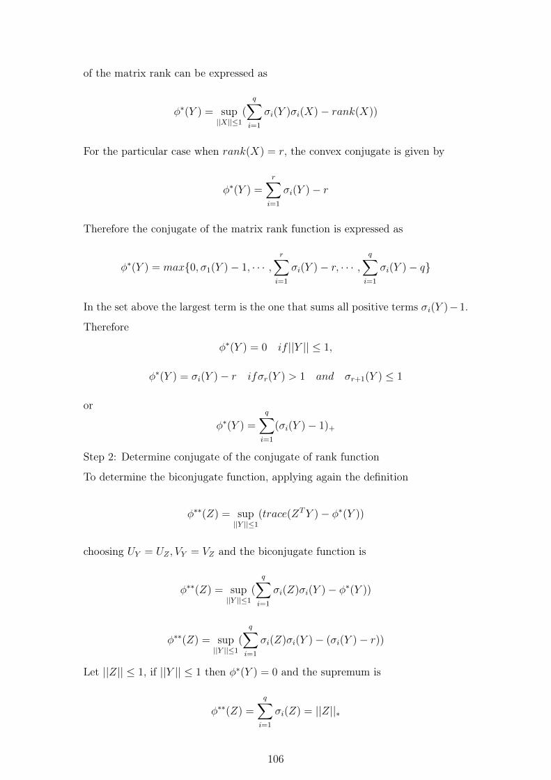
of the matrix rank can be expressed as
φ∗(Y ) = sup||X||≤1
(
q�
i=1
σi(Y )σi(X)− rank(X))
For the particular case when rank(X) = r, the convex conjugate is given by
φ∗(Y ) =r�
i=1
σi(Y )− r
Therefore the conjugate of the matrix rank function is expressed as
φ∗(Y ) = max{0, σ1(Y )− 1, · · · ,r�
i=1
σi(Y )− r, · · · ,q�
i=1
σi(Y )− q}
In the set above the largest term is the one that sums all positive terms σi(Y )−1.
Therefore
φ∗(Y ) = 0 if ||Y || ≤ 1,
φ∗(Y ) = σi(Y )− r ifσr(Y ) > 1 and σr+1(Y ) ≤ 1
or
φ∗(Y ) =
q�
i=1
(σi(Y )− 1)+
Step 2: Determine conjugate of the conjugate of rank function
To determine the biconjugate function, applying again the definition
φ∗∗(Z) = sup||Y ||≤1
(trace(ZTY )− φ∗(Y ))
choosing UY = UZ , VY = VZ and the biconjugate function is
φ∗∗(Z) = sup||Y ||≤1
(
q�
i=1
σi(Z)σi(Y )− φ∗(Y ))
φ∗∗(Z) = sup||Y ||≤1
(
q�
i=1
σi(Z)σi(Y )− (σi(Y )− r))
Let ||Z|| ≤ 1, if ||Y || ≤ 1 then φ∗(Y ) = 0 and the supremum is
φ∗∗(Z) =q�
i=1
σi(Z) = ||Z||∗
106
If ||Y || > 1 then the expression can be re-written as:
φ∗∗(Z) =q�
i=1
σi(Y )σi(Z)−r�
i=1
(σi(Y )− 1)
Adding and subtracting the termq�
i=1
σi(Z) and grouping the terms
φ∗∗(Z) =q�
i=1
σi(Y )σi(Z)−r�
i=1
(σi(Y )− 1)−q�
i=1
σi(Z) +
q�
i=1
σi(Z)
φ∗∗(Z) =r�
i=1
(σi(Y )− 1)(σi(Z)− 1) +
q�
i=r+1
(σi(Y )− 1)σi(Z) +
q�
i=1
σi(Z)
which leads to
φ∗∗(Z) <q�
i=1
σi(Z)
Therefore
φ∗∗(Z) = ||Z||∗
over the set {Z; ||Z|| ≤ 1}. Thus, over this set, ||Z||∗ is the convex envelope of
the function rank(Z).
107
LIST OF PAPERS BASED ON THESIS
Papers in Refereed International Journals
1. M.Vanidevi, and N.Selvaganesan. Channel Estimation for Finite Scatterers
Massive Multi-User MIMO System. Circuits, Systems, and Signal Process-
ing - Springer, Vol.36, No.9, pp 3761-3777, 2017.
2. M.Vanidevi, N.Selvaganesan. Fast Iterative WSVT Algorithm in WNN Min-
imization Problem for Multi-user Massive MIMO Channel Estimation. In-
ternational Journal of Communication Systems - Wiley, Vol.31, No.1, 2018
.
Presentations in Conferences
1. M.Vanidevi, N.Selvaganesan, etal "Tracking of MIMO channel in the pres-
ence of unknown interference", in India Conference (INDICON), 2014 An-
nual IEEE, 2014.
2. M.Vanidevi, N.Selvaganesan, etal,"Impact of spatial correlation and channel
estimation error on Precoded MIMO systems", 2014 International Confer-
ence on Signal Propagation and Computer Technology (ICSPCT 2014).
108