Weitzenbock and Clark-Oconedecompositions for differential forms on the

space of normal martingales∗

Nicolas PrivaultDivision of Mathematical Sciences

School of Physical and Mathematical Sciences

Nanyang Technological University

21 Nanyang Link

Singapore 637371

November 28, 2015

Abstract

We present a framework for the construction of Weitzenbock and Clark-Ocone formulae for differential forms on the probability space of a normal mar-tingale. This approach covers existing constructions based on Brownian motion,and extends them to other normal martingales such as compensated Poissonprocesses. It also applies to the path space of Brownian motion on a Lie groupand to other geometries based on the Poisson process. Classical results suchas the de Rham-Hodge-Kodaira decomposition and the vanishing of harmonicdifferential forms are extended in this way to finite difference operators by twodistinct approaches based on the Weitzenbock and Clark-Ocone formulae.

Keywords : de Rham-Hodge-Kodaira decomposition, differential forms, Weitzenbock

identity, Clark-Ocone formula, normal martingales, Malliavin calculus.

Classification: 60H07, 60J65, 58J65, 58A10.

1 Introduction

Vanishing theorems for harmonic forms on Riemannian manifolds can be proved by

the Bochner method, which involves the Weitzenbock formula and relates the Hodge

∗Numerous comments and suggestions by Yuxin Yang on this paper are gratefully acknowledged.

1

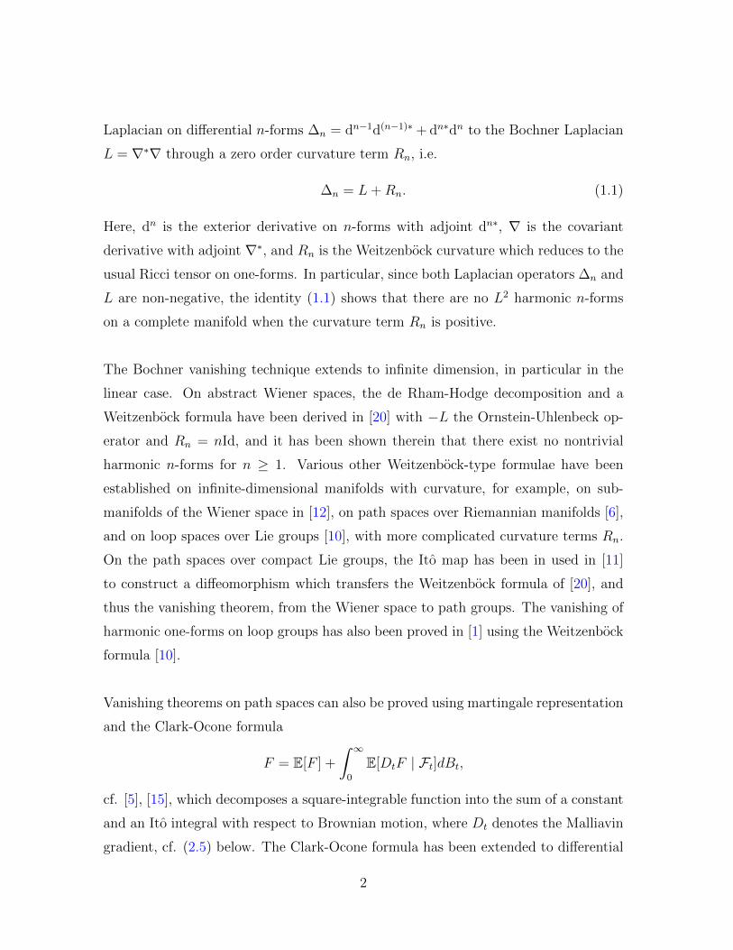
Laplacian on differential n-forms ∆n = dn−1d(n−1)∗ + dn∗dn to the Bochner Laplacian

L = ∇∗∇ through a zero order curvature term Rn, i.e.

∆n = L+Rn. (1.1)

Here, dn is the exterior derivative on n-forms with adjoint dn∗, ∇ is the covariant

derivative with adjoint ∇∗, and Rn is the Weitzenbock curvature which reduces to the

usual Ricci tensor on one-forms. In particular, since both Laplacian operators ∆n and

L are non-negative, the identity (1.1) shows that there are no L2 harmonic n-forms

on a complete manifold when the curvature term Rn is positive.

The Bochner vanishing technique extends to infinite dimension, in particular in the

linear case. On abstract Wiener spaces, the de Rham-Hodge decomposition and a

Weitzenbock formula have been derived in [20] with −L the Ornstein-Uhlenbeck op-

erator and Rn = nId, and it has been shown therein that there exist no nontrivial

harmonic n-forms for n ≥ 1. Various other Weitzenbock-type formulae have been

established on infinite-dimensional manifolds with curvature, for example, on sub-

manifolds of the Wiener space in [12], on path spaces over Riemannian manifolds [6],

and on loop spaces over Lie groups [10], with more complicated curvature terms Rn.

On the path spaces over compact Lie groups, the Ito map has been in used in [11]

to construct a diffeomorphism which transfers the Weitzenbock formula of [20], and

thus the vanishing theorem, from the Wiener space to path groups. The vanishing of

harmonic one-forms on loop groups has also been proved in [1] using the Weitzenbock

formula [10].

Vanishing theorems on path spaces can also be proved using martingale representation

and the Clark-Ocone formula

F = E[F ] +

∫ ∞0

E[DtF | Ft]dBt,

cf. [5], [15], which decomposes a square-integrable function into the sum of a constant

and an Ito integral with respect to Brownian motion, where Dt denotes the Malliavin

gradient, cf. (2.5) below. The Clark-Ocone formula has been extended to differential

2

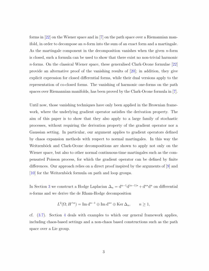
forms in [22] on the Wiener space and in [7] on the path space over a Riemannian man-

ifold, in order to decompose an n-form into the sum of an exact form and a martingale.

As the martingale component in the decomposition vanishes when the given n-form

is closed, such a formula can be used to show that there exist no non-trivial harmonic

n-forms. On the classical Wiener space, these generalised Clark-Ocone formulae [22]

provide an alternative proof of the vanishing results of [20]; in addition, they give

explicit expression for closed differential forms, while their dual versions apply to the

representation of co-closed forms. The vanishing of harmonic one-forms on the path

spaces over Riemannian manifolds, has been proved by the Clark-Ocone formula in [7].

Until now, those vanishing techniques have only been applied in the Brownian frame-

work, where the underlying gradient operator satisfies the derivation property. The

aim of this paper is to show that they also apply to a large family of stochastic

processes, without requiring the derivation property of the gradient operator nor a

Gaussian setting. In particular, our argument applies to gradient operators defined

by chaos expansion methods with respect to normal martingales. In this way the

Weitzenbock and Clark-Ocone decompositions are shown to apply not only on the

Wiener space, but also to other normal continuous-time martingales such as the com-

pensated Poisson process, for which the gradient operator can be defined by finite

differences. Our approach relies on a direct proof inspired by the arguments of [9] and

[10] for the Weitzenbock formula on path and loop groups.

In Section 3 we construct a Hodge Laplacian ∆n = dn−1d(n−1)∗+ dn∗dn on differential

n-forms and we derive the de Rham-Hodge decomposition

L2(Ω;H∧n) = Im dn−1 ⊕ Im dn∗ ⊕Ker ∆n, n ≥ 1,

cf. (3.7). Section 4 deals with examples to which our general framework applies,

including chaos-based settings and a non-chaos based constructions such as the path

space over a Lie group.

3

In Theorem 5.2 we prove the Weitzenbock identity

∆n = nIdH∧n +∇∗∇, n ≥ 1,

and in Proposition 5.1 we show the vanishing of harmonic forms Ker ∆n = 0, from

which the de Rham-Hodge decomposition

L2(Ω;H∧n) = Im dn−1 ⊕ Im dn∗, n ≥ 1,

follows. This result is also derived in Corollary 6.2 from the Clark-Ocone formula of

Theorem 6.1, showing the complementarity of the two approaches.

It can be shown in addition that this method goes beyond chaos expansions and en-

compasses other natural geometries in addition to the path space over a Lie group

described in Section 4, for example on the Poisson space over the half line IR+, cf.

[19], in which case the gradient operator has the derivation property.

In [2], [3], n-differential forms on the configuration space over a Riemannian manifold

under a Poisson random measure have been constructed in a different way by a lifting

of the underlying differential structure on the manifold to the configuration space. We

also refer the reader to [4] for a different approach to the construction of the Hodge

decomposition on abstract metric spaces.

This paper is organized as follows. Sections 2 and 3 introduce the general framework

of differential and divergence operators on functions and differential forms, includ-

ing duality and commutation relations. Section 4 describes a number of examples to

which this framework applies, while Sections 5 and 6 present the main results on the

Weitzenbock identity and the generalised Clark-Ocone formulae, respectively, includ-

ing the vanishing of harmonic forms. The examples of Section 4, which range from

normal martingales to Lie-group valued Brownian motion, are revisited one by one in

the frameworks of Sections 5 and 6. The appendix contains the proofs of the main

results.

4

2 Differential forms and exterior derivative

In this section we introduce an abstract gradient and divergence framework based on

a probability space (Ω,F ,P) and an algebra S ⊂ L2(Ω) for the pointwise product of

random variables, dense in L2(Ω).

Deterministic forms

We fix a measure space (X, σ) and we consider a linear space H of IRd-valued func-

tions, dense in L2(X, IRd), d ≥ 1, and endowed with the inner product induced from

L2(X, IRd). Denote by H⊗n the n-th tensor power of H, and by Hn, resp. H∧n, its

subspaces of symmetric, resp. skew-symmetric tensors, completed using the inherited

Hilbert space cross norm. The exterior product ∧ is defined as

h1 ∧ · · · ∧ hn := An(h1 ⊗ · · · ⊗ hn), h1, . . . , hn ∈ H, (2.1)

where An denotes the antisymmetrization map on n-tensors given by

An(h1 ⊗ · · · ⊗ hn) =∑σ∈Σn

sign(σ)(hσ(1) ⊗ · · · ⊗ hσ(n)), (2.2)

and the summation is over n! elements of the symmetric group Σn consisting of all

permutations of 1, . . . , n. We also equip H∧n with the inner product

〈fn, gn〉H∧n :=1

n!

∫X

· · ·∫X

〈fn(x1, . . . , xn), gn(x1, . . . , xn)〉(IRd)⊗nσ(dx1) · · ·σ(dxn)

=1

n!〈fn, gn〉H⊗n , fn, gn ∈ H∧n,

so that we have in particular

〈h1 ∧ · · · ∧ hn, k1 ∧ · · · ∧ kn〉H∧n

:=1

n!

∫X

· · ·∫X

〈An(h1 ⊗ · · · ⊗ hn),An(k1 ⊗ · · · ⊗ kn)〉(IRd)⊗nσ(dx1) · · ·σ(dxn)

=1

n!

∫X

· · ·∫X

⟨ ∑σ∈Σn

sign(σ)(hσ(1) ⊗ · · · ⊗ hσ(n)),∑η∈Σn

sign(η)(kη(1) ⊗ · · · ⊗ kη(n))⟩

(IRd)⊗nσ(dx1) · · ·σ(dxn)

5

=∑σ∈Σn

sign(σ)

∫X

· · ·∫X

〈hσ(1) ⊗ · · · ⊗ hσ(n), k1 ⊗ · · · ⊗ kn)〉(IRd)⊗nσ(dx1) · · ·σ(dxn)

=∑σ∈Σn

sign(σ)

∫X

· · ·∫X

〈hσ(1), k1〉IRd · · · 〈hσ(n), kn〉IRdσ(dx1) · · ·σ(dxn)

= det((〈hi, kj〉H)1≤i,j≤n).

h1, . . . , hn, k1, . . . , kn ∈ H.

Covariant derivative

In the sequel we will use a covariant derivative operator

∇ : H −→ H ⊗H

h 7−→ ∇h = (∇xh)x∈X ,

where ∇xh ∈ IRd ⊗H, x ∈ X, is defined from the relation

〈∇xh, k〉H := 〈∇h, k〉H(x) ∈ IRd, x ∈ X, h, k ∈ H.

We will extend the definition of ∇ to an operator

∇ : H∧n −→ H ⊗H∧n

on differential forms in H∧n, by the following steps.

(i) Let

∇(l)x (h1 ∧ · · · ∧ hn) ∈ H ∧ · · · ∧H︸ ︷︷ ︸

l-1 times

∧(IRd ⊗H) ∧H ∧ · · · ∧H︸ ︷︷ ︸n-l times

as

∇(l)x (h1 ∧ · · · ∧ hn) := h1 ∧ · · · ∧ hl−1 ∧∇xhl ∧ hl+1 ∧ · · · ∧ hn, x ∈ X,

l = 1, . . . , n.

(ii) We define ∇x(h1 ∧ · · · ∧ hn) in IRd ⊗H∧n, x ∈ X, as

∇x(h1 ∧ · · · ∧ hn) :=n∑j=1

∇(j)x (h1 ∧ · · · ∧ hn) (2.3)

6

=n∑j=1

h1 ∧ · · · ∧ hj−1 ∧∇xhj ∧ hj+1 ∧ · · · ∧ hn,

by canonically identifying the space

H ∧ · · · ∧H︸ ︷︷ ︸l-1 times

∧(IRd ⊗H) ∧H ∧ · · · ∧H︸ ︷︷ ︸n-l times

to IRd ⊗H∧n, for l = 1, . . . , n.

Given g ∈ H we also define ∇g(h1 ∧ · · · ∧ hn) ∈ H∧n by

∇g(h1 ∧ · · · ∧ hn) :=

∫X

〈g(x),∇x(h1 ∧ · · · ∧ hn)〉IRdσ(dx)

=n∑j=1

∫X

〈g(x), (h1 ∧ · · · ∧ hj−1 ∧∇xhj ∧ hj+1 ∧ · · · ∧ hn)〉IRdσ(dx)

=n∑j=1

(h1 ∧ · · · ∧ hj−1 ∧∇ghj ∧ hj+1 ∧ · · · ∧ hn).

Exterior derivative - deterministic forms

We now define the exterior derivative on n-forms un ∈ H∧n by

〈dnun, h1∧· · ·∧hn+1〉H∧(n+1) :=n+1∑k=1

(−1)k−1〈∇hkun, h1∧· · ·∧hk−1∧hk+1∧· · ·∧hn+1〉H∧n ,

(2.4)

where h1, . . . , hn+1 ∈ H, i.e. dn =1

n!An+1∇, and the (n + 1)-form dn(h1 ∧ · · · ∧ hn)

is given by

dnxn+1((h1 ∧ · · · ∧ hn)(x1, . . . , xn)) = dn(h1 ∧ · · · ∧ hn)(x1, . . . , xn+1)

=n+1∑j=1

(−1)j−1∇xj(h1 ∧ · · · ∧ hn)(x1, . . . , xj−1, xj+1, . . . , xn+1)

=n+1∑j=1

(−1)j−1

n∑i=1

∇(i)xj

(h1 ∧ · · · ∧ hn)(x1, . . . , xj−1, xj+1, . . . , xn+1)

=n+1∑j=1

(−1)j−1

n∑i=1

(h1 ∧ · · · ∧ ∇xjhi ∧ · · · ∧ hn)(x1, . . . , xj−1, xj+1, . . . , xn+1).

7

Random forms

In the sequel we will need a linear gradient operator

D : S −→ L2(Ω;H)

F 7−→ DF = (DxF )x∈X (2.5)

acting on random variables in S.

We work on the space S ⊗H∧n of elementary (random) n-forms that can be written

as linear combinations of terms for the form

un = F ⊗ h ∈ S ⊗H∧n, F ∈ S, h ∈ H∧n. (2.6)

The operator D is extended to un ∈ S ⊗H∧n as in (2.6) by the pointwise equality

Dxun := (DxF )⊗ (h1 ∧ · · · ∧ hn), x ∈ X, (2.7)

i.e. Dun ∈ S ⊗H⊗H∧n. We also extend ∇ to random forms un = F ⊗ fn ∈ S ⊗H∧n

by defining ∇un ∈ S ⊗H ⊗H∧n as

∇y(un(x1, . . . , xn)) := (DyF )⊗ fn(x1, . . . , xn) + F ⊗∇yfn(x1, . . . , xn)

= (DyF )⊗ fn(x1, . . . , xn) + F ⊗n∑l=1

∇(l)y fn(x1, . . . , xn),

x1, . . . , xn, y ∈ X. In particular for n = 1, ∇ extends to stochastic processes (or

one-forms) as

∇x(u1(y)) = ∇x(F ⊗ f1(y)) = (DxF )⊗ f1(y) + F ⊗∇xf1(y),

with u1 = F ⊗ f1 ∈ S ⊗H.

Lie bracket and vanishing of torsion

The Lie bracket f, g of f, g ∈ H, is defined to be the unique element w of H

satisfying

(DfDg −DgDf )F = DwF, F ∈ S, (2.8)

8

where

DfF := 〈f,DF 〉H , f ∈ H, F ∈ Dom (D),

and is extended to u, v ∈ S ⊗H by

Fu,Gv(x) = FGu, v(x) + v(x)FDuG− u(x)GDvF, x ∈ X,

u, v ∈ H, F,G ∈ S. In the sequel we will make the following assumption.

(A1) Vanishing of torsion. The connection defined by ∇ has a vanishing torsion,

i.e. we have

u, v = ∇uv −∇vu, u, v ∈ S ⊗H. (A1)

From (2.8) the vanishing of torsion Assumption (A1) can be written as∫X

∫X

〈(DxDyF −DyDxF ), f(x)⊗ g(y)〉IRd⊗IRdσ(dx)σ(dy) (2.9)

=

∫X

∫X

〈∇yg(x), DxF ⊗ f(y)〉IRd⊗IRdσ(dx)σ(dy)

−∫X

∫X

〈∇yf(x), DxF ⊗ g(y)〉IRd⊗IRdσ(dx)σ(dy), F ∈ S, f, g ∈ H.

Exterior derivative - random forms

From Assumption (A1) we may now define the (n+ 1)-form dnun as

dnun(x1, . . . , xn+1) := dnxn+1(un(x1, . . . , xn))

=1

n!An+1(∇·un)(x1, . . . , xn+1)

= (D·F ∧ fn)(x1, . . . , xn+1) +1

n!F ⊗An+1(∇·fn)(x1, . . . , xn+1),

which is also equal to

n+1∑j=1

(−1)j−1∇xjun(x1, . . . , xj−1, xj+1, . . . , xn+1)

in H∧(n+1), for un ∈ S ⊗H∧n of the form (2.6). In other words, on elementary forms

we have

dnxn+1(F ⊗ h1 ∧ · · · ∧ hn(x1, . . . , xn)) = dn(F ⊗ h1 ∧ · · · ∧ hn)(x1, . . . , xn+1) (2.10)

9

= ((D·F ) ∧ h1 ∧ · · · ∧ hn)(x1, . . . , xn+1) + F ⊗ dn(h1 ∧ · · · ∧ hn)(x1, . . . , xn+1).

In particular, for n = 0 we have

d0xF = ∇xF = DxF, F ∈ S ⊗H∧0 = S.

and for n = 1,

d1(F⊗h1)(x1, x2) = d1x2

(F⊗h1(x1)) = F⊗d1x1h1(x2)+(Dx1F )⊗h(x2)−Dx2F⊗h(x1).

We also note that

dn(S ⊗H∧n) ⊂ Dom (dn+1), n ∈ N. (2.11)

Assumption (A1) and the invariant formula for differential forms (see e.g. Prop. 3.11

page 36 of [13]) also show that we have

dn+1dn = 0, n ∈ N, (2.12)

which implies

Im dn ⊂ Ker dn+1 ⊂ Dom (dn+1), n ∈ N. (2.13)

3 Divergence of n-forms and duality

In this section we consider a divergence operator

δ : S ⊗H −→ L2(Ω),

u = (u(x))x∈X 7−→ δ(u)

acting on stochastic processes, and extended to elementary n-forms by letting

δ(h1 ∧ · · · ∧ hn)

:=1

n

n∑j=1

(−1)j−1δ(hj)⊗ (h1 ∧ · · · ∧ hj−1 ∧ hj+1 ∧ · · · ∧ hn) ∈ S ⊗H∧(n−1),

and to simple elements u ∈ S ⊗H∧n of the form (2.6) by

δ(un)(x1, . . . , xn−1) := δ(un(·, x1, . . . , xn−1)) (3.1)

= δ(F ⊗ (h1 ∧ · · · ∧ hn))(x1, . . . , xn−1)

=1

n

n∑j=1

(−1)j−1δ(F ⊗ hj)⊗ (h1 ∧ · · · ∧ hj−1 ∧ hj+1 ∧ · · · ∧ hn)(x1, . . . , xn−1).

10

Divergence of random forms

The divergence operator dn∗ on (n+ 1)-forms un+1 = F ⊗ fn+1 ∈ S ⊗H∧(n+1) of the

form (2.6) is defined by

dn∗un+1(x1, . . . , xn) := δ(F ⊗ fn+1(·, x1, . . . , xn))− F trace(∇·fn+1(·, x1, . . . , xn))

where

trace(∇·fn+1(·, x1, . . . , xn)) :=

∫ ∞0

Tr∇xfn+1(x, x1, . . . , xn)σ(dx)

and Tr denotes the trace on IRd ⊗ IRd, i.e. we have

dn∗un+1(x1, . . . , xn)

= δ(F ⊗ fn+1(·, x1, . . . , xn))− F∫ ∞

0

Tr∇xfn+1(x, x1, . . . , xn)σ(dx), (3.2)

which belongs to S ⊗H∧n from (3.1), n ≥ 1, and

d0∗u1 = δ(u1), u1 ∈ S ⊗H, (3.3)

when n = 0 since ∇xf1(x) = 0.

Duality relations

We will make the following assumptions on δ, D and ∇:

(A2) The operators D and δ satisfy the duality relation

E[〈DF, u〉H ] = E[Fδ(u)], F ∈ Dom (D), u ∈ Dom (δ). (A2)

The above duality condition (A2) implies that the operators D and δ are clos-

able, cf. Proposition 3.1.2 of [18], and the operators D and δ are extended to

their respective closed domains Dom (D) and Dom (δ).

(A3) The operator ∇ satisfies the condition∫Xn+1

〈gn+1(x1, . . . , xn+1),∇x1fn(x2, . . . , xn+1)〉(IRd)⊗(n+1)σ(dx1) · · ·σ(dxn+1) =

11

−∫Xn+1

〈Tr∇xgn+1(x, x1, . . . , xn), fn(x1, . . . , xn)〉(IRd)⊗nσ(dx1) · · ·σ(dxn)σ(dx),

(A3)

fn ∈ H⊗n, gn+1 ∈ H⊗(n+1), n ≥ 1.

The compatibility condition (A3) is weaker than the usual compatibility of ∇with the metric 〈·, ·〉H , which reads

〈∇xfn, gn〉H⊗n = −〈fn,∇xgn〉H⊗n , x ∈ X, (3.4)

fn, gn ∈ H⊗n. Indeed, when applying (3.4) to fn+1(x, ·) ∈ H⊗n and gn ∈ H⊗n,

x ∈ X, n ≥ 1, we get∫Xn+1

〈Tr∇xfn+1(x, x1, . . . , xn), gn(x1, . . . , xn)〉(IRd)⊗nσ(dx1) · · ·σ(dxn)σ(dx)

=d∑

k=1

∫Xn+1

〈(∇xf(k)n+1(x, x1, . . . , xn))(k), gn(x1, . . . , xn)〉(IRd)⊗nσ(dx1) · σ(dxn)σ(dx)

= −d∑

k=1

∫Xn+1

〈f (k)n+1(x, x1, . . . , xn), (∇xgn(x1, . . . , xn))(k)〉(IRd)⊗nσ(dx1) · σ(dxn)σ(dx)

= −∫Xn+1

〈fn+1(x, x1, . . . , xn),∇xgn(x1, . . . , xn)〉(IRd)⊗(n+1)σ(dx1) · σ(dxn)σ(dx),

where f(k)n+1(x, x1, . . . , xn) denotes the k-th component in IRd of the first com-

ponent of fn+1(x, x1, . . . , xn) in (IRd)⊗(n+1). In this sense, Assumption (A3) is

automatically satisfied in all settings which incorporate the compatibility (3.4)

with 〈·, ·〉.

Proposition 3.1. (Duality). Under Assumptions (A1)-(A3), for any un ∈ S ⊗H∧n

and vn+1 ∈ S ⊗H∧(n+1) we have

〈dnun, vn+1〉L2(Ω,H∧(n+1)) = 〈un, dn∗vn+1〉L2(Ω,H∧n). (3.5)

As above we note that the duality (3.5) implies the closability of both dn and dn∗vn+1,

which are extended to their closed domains Dom (dn) and Dom (dn∗), n ∈ N, by the

same argument as in Proposition 3.1.2 of [18]. When n = 0, the statement of Propo-

sition 3.1 reduces to (A2).

12

The proof of Proposition 3.1 is postponed to the appendix. In the case of one-forms

it reads

〈d1t2

(Ff1(t1)), Gg2(t1, t2)〉L2(Ω,H∧2)

=

⟨∇t1

(F

2f1(t2)

), Gg2(t1, t2)

⟩L2(Ω,H⊗2)

−⟨∇t2

(F

2f1(t1)

), Gg2(t1, t2)

⟩L2(Ω,H⊗2)

=

⟨Dt1

F

2f1(t2), Gg2(t1, t2)

⟩L2(Ω,H⊗2)

−⟨Dt2

F

2f1(t1), Gg2(t1, t2)

⟩L2(Ω,H⊗2)

+

⟨F

2∇t1f1(t2), Gg2(t1, t2)

⟩L2(Ω,H⊗2)

−⟨F

2∇t2f1(t1), Gg2(t1, t2)

⟩L2(Ω,H⊗2)

=

⟨F

2f1(t2), δ(Gg2(·, t2))

⟩L2(Ω,H)

−⟨F

2f1(t1), δ(Gg2(t1, ·))

⟩L2(Ω,H)

−⟨F

2f1(t2), G

∫ ∞0

Tr∇tg2(t, t2)dt

⟩L2(Ω,H)

−⟨F

2f1(t1), G

∫ ∞0

Tr∇tg2(t1, t)dt

⟩L2(Ω,H)

=

⟨F

2f1(t2), δ(Gg2(·, t2))

⟩L2(Ω,H)

+

⟨F

2f1(t1), δ(Gg2(·, t1))

⟩L2(Ω,H)

−⟨F

2f1(t2), G

∫ ∞0

Tr∇tg2(t, t2)dt

⟩L2(Ω,H)

+

⟨F

2f1(t1), G

∫ ∞0

Tr∇tg2(t, t1)dt

⟩L2(Ω,H)

= 〈Ff1(t1), δ(Gg2(·, t1))〉L2(Ω,H) −⟨Ff1(t1), G

∫ ∞0

Tr∇tg2(t, t1)dt⟩L2(Ω,H)

= 〈Ff1(t1), d1∗(Gg2)(t1)〉L2(Ω,H), F,G ∈ S, f1 ∈ H, g2 ∈ H∧2.

As in (A2) above, the duality (3.5) shows that dn extends to a closed operator

dn : Dom (dn) −→ L2(Ω;H∧(n+1))

with domain Dom (dn) ⊂ L2(Ω;H∧n), and dn∗, n ∈ N, extends to a closed operator

dn∗ : Dom (dn∗) −→ L2(Ω;H∧n)

with domain Dom (dn∗) ⊂ L2(Ω;H∧(n+1)), by the same argument as in Proposi-

tion 3.1.2 of [18].

In addition, by the coboundary condition (2.12) and the duality (3.5) we find

dn∗d(n+1)∗ = 0, n ∈ N.

13

Based on (2.13) we define the Hodge Laplacian on differential n-forms as

∆n = dn−1d(n−1)∗ + dn∗dn, (3.6)

and call harmonic n-forms the elements of the kernel Ker ∆n of ∆n. By (2.12)-(2.13)

and Proposition 3.1 we have the de Rham-Hodge decomposition

L2(Ω;H∧n) = Im dn−1 ⊕ Im dn∗ ⊕Ker ∆n, n ≥ 1. (3.7)

Indeed, the spaces of exact and co-exact forms Im dn−1 and Im dn∗ are mutually

orthogonal by (2.12) and the duality of Proposition 3.1. Moreover, the orthogonal

complement (Ker d(n−1)∗) ∩ (Ker dn) of Im dn−1 ⊕ Im dn∗ in L2(Ω;H∧n) is made of

n-forms un that are both closed (dnun = 0) and co-closed (d(n−1)∗un = 0), hence it is

contained in (and equal to) Ker ∆n by (3.6).

Intertwinning relations

The statements and proofs of both the Weitzenbock identity and Clark-Ocone formula

in the sequel will also require the following conditions. We assume that

(A4) the operator ∇ satisfies

∇xf(y) · ∇yf(x) = 0, σ(dx)σ(dy)− a.e., f ∈ H, (A4)

i.e. σ(dx)σ(dy)− a.e. we have ∇xf(y) = 0 or ∇yf(x) = 0.

(A5) Intertwinning relation. For all u ∈ S ⊗H of the form u = F ⊗ f we have

〈g,Dδ(u)〉H = 〈g, u〉H + δ(∇gu) + 〈DF,∇fg〉H , g ∈ H. (A5)

We make the following remarks.

Remark 3.1. (i) When ∇ = 0 on H, Assumption (A5) reads

Dxδ(u) = u(x) + δ(Dxu), x ∈ X,

for all u = F ⊗ f ∈ S ⊗H.

14

(ii) Under the torsion free Assumption (A1), Relation (2.9) shows that (A5) reads

Dxδ(u) = u(x) + δ(∇xu) + 〈DDxF, f〉H −〈DxDF, f〉H + 〈D·F,∇xf(·)〉H , (3.8)

u = F ⊗ f ∈ S ⊗H, x ∈ X.

(iii) As a consequence of (3.8), Assumption (A5) simplifies to

Dxδ(h) = h(x) + δ(∇xh), x ∈ X, h ∈ H. (A5’)

when D satisfies the Leibniz rule of derivation

Dx(FG) = FDxG+GDxF, F,G ∈ S, x ∈ X. (3.9)

This will be the case in examples where ∇ does not vanish on H.

(iv) When D has the derivation property (3.9), Relation (3.2) rewrites as the diver-

gence formula

dn∗un+1(x1, . . . , xn)

= Fδ(fn+1(·, x1, . . . , xn))−∫ ∞

0

Tr∇x(Ffn+1(x, x1, . . . , xn))σ(dx),

un+1 = F ⊗ fn+1 ∈ S ⊗H∧(n+1).

Proof. We only prove (iii) and (iv).

(iii) First, we note that the duality condition (A2) and the Leibniz rule (3.9) imply

δ(Fh) = Fδ(h)− 〈DF, h〉H , F ∈ S, h ∈ H. (3.10)

Hence by (A5’) and (3.9) we have

Dxδ(Fh) = Dx(Fδ(h)− 〈DF, h〉H)

= δ(h)DxF + FDxδ(h)−Dx〈DF, h〉H

= δ(h)DxF + Fh(x) + Fδ(∇xh)−Dx〈DF, h〉H

= Fh(x) + δ(hDxF ) + 〈DDxF, h〉H + δ(F∇xh) + 〈D·F,∇xh(·)〉H − 〈DxDF, h〉H

= u1(x) + δ(∇xu1) + 〈DDxF, h〉H − 〈DxDF, h〉H + 〈D·F,∇xh(·)〉H .

The converse statement is immediate.

(iv) This is a consequence of (3.2) and the divergence formula (3.10).

15

4 Examples

In this section we consider examples of frameworks satisfying Assumptions (A1)-(A5).

Commutative examples - chaos expansions

We start by considering a family of examples based on chaos expansions, in which we

take ∇h = 0 for all h ∈ H. Here (X, σ) is a measure space, we take H = L2(X, σ) and

d ≥ 1 and we assume that the chaos decomposition holds, i.e. every F ∈ L2(Ω,F , P )

can be decomposed into a series

F =∞∑n=0

In(fn), fn ∈ Hn,

of multiple stochastic integrals, where I0(f0) = E[F ] and for all n ≥ 1, the multiple

stochastic integral In : Hn → L2(Ω) satisfies the isometry condition

〈In(fn), Im(gm)〉L2(Ω) = n!1n=m〈fn, gm〉Hn , n,m ≥ 1.

In this case the space S is made of the finite chaos expansions

S =

C +

n∑k=1

Ik(fk), fk ∈ L2(X)k, k = 1, . . . , n, n ≥ 1, C ∈ IR

,

the operator

D : Dom(D) −→ L2(Ω×X, dP × σ(dx))

is defined by

DxIn(fn) := nIn−1(fn(∗, x)), dP × σ(dx)− a.e., n ∈ N. (4.1)

On the other hand,

δ : Dom (δ) −→ L2(Ω),

is defined on processes of the form (In(fn+1(∗, t)))t∈IR+ as

δ(In(fn+1(∗, ·))) := In+1(fn+1), n ∈ N, (4.2)

where fn+1 denotes the symmetrization of fn+1 ∈ Hn ⊗ H in (n + 1) variables. In

this chaos expansion framework we have ∇ = D and ∇f = 0 for all f ∈ H, hence

16

Assumptions (A1) and (A3)-(A4) are obviously satisfied and the exterior derivative d

is defined by the skew-symmetrisation of D, i.e. (2.10) becomes

dnxn+1(F ⊗ h1 ∧ · · · ∧ hn(x1, . . . , xn)) = ((D·F ) ∧ h1 ∧ · · · ∧ hn)(x1, . . . , xn+1), (4.3)

x1, . . . , xn+1 ∈ X. As for Assumptions (A2) and (A5) we have the following:

(A2) the duality relation holds in the general framework of chaos expansions; see,

e.g., Proposition 4.1.3 of [18];

(A5) given that ∇ = D, the commutation relation (A5) holds for u ∈ S ⊗ H, see,

e.g., Proposition 4.1.4 of [18].

Note that here, Relations (2.12)-(2.13) hold by the definition (4.3) of the exterior

derivative d and the symmetry of second derivative.

Next, we consider some specific examples based on chaos expansions.

Example 1.1 - Poisson random measures

On the probability space of a Poisson random measure ω(dx) with σ-finite intensity

measure σ(dx) on X, In(f) is the multiple compensated Poisson stochastic integral

In(fn) :=

∫∆n

fn(x1, . . . , xn)(ω(dx1)− σ(dx1)) · · · (ω(dxn)− σ(dxn))

of the symmetric function fn ∈ Hn with respect to ω(dx), where

∆n = (x1, . . . , xn) ∈ Xn : xi 6= xj, 1 ≤ i < j ≤ n.

Here the operator Dx defined in (4.1) acts by finite differences and addition of a

configuration point at x ∈ X, i.e.

DxF (ω) = F (ω ∪ x)− F (ω), x ∈ X,

where ω ∪x represents the addition of the point x to the point configuration ω, see

e.g., Proposition 6.4.7 of [18]. Being a finite difference operator, D does not have the

17

derivation property. We refer the reader to § 6.5 of [18] and references therein for the

expression of δ defined in (4.2) in this setting.

Example 1.2 - Normal martingales

When X = IR+, chaos-based examples satisfying the above conditions (A1)-(A5)

include normal martingales having the chaos representation property (CRP). An

(Ft)t∈IR+-martingale (Mt)t∈IR+ on a filtered probability space (Ω, (Ft)t∈IR+ , P ) is called

a normal martingale under P if

E[(Mt −Ms)2 | Fs] = t− s, 0 ≤ s ≤ t,

see, e.g., [18] and references therein. Here we also assume that (Mt)t∈IR+ has the

chaos representation property (CRP), and the multiple stochastic integral In(fn) of

fn ∈ L2(IR+)n with respect to (Mt)t∈IR+ is given by

In(fn) = n!

∫ ∞0

∫ tn

0

· · ·∫ t2

0

fn(t1, . . . , tn)dMt1 · · · dMtn , n ≥ 1.

Examples of normal martingales satisfying the CRP include the Brownian motion and

the compensated Poisson process, both of which we discuss in more details below, as

well as certain processes with non-independent increments such as the Azema mar-

tingales, for which the explicit expression of the gradient D is generally unknown; see

[8] and § 2.10 of [18].

Example 1.2-a) - Brownian motion

When X = IR+ and (Mt)t∈IR+ is the standard Brownian motion with respect to its own

filtration (Ft)t∈IR+ , it is usual to take S as the space of smooth cylindrical functionals

of the form

F = f(I1(h1), . . . , I1(hn)), h1, . . . , hn ∈ H, f ∈ C∞b (IRn),

on which the gradient D is defined by

DF =n∑i=1

hi∂if(I1(h1), . . . , I1(hn)), (4.4)

18

e.g., see Definition 1.2.1 in [14]. Here, D is a derivation, whose adjoint δ is also called

the Skorohod integral, the multiple integrals In are the well-known multiple Ito inte-

grals, and (Ft)t∈IR+ is the standard Brownian filtration.

Example 1.2-b) - Standard Poisson process

In the special case X = IR+ we can define a standard compensated Poisson process

(Mt)t∈IR+ as (Mt)t∈IR+ := (Nt − t)t∈IR+ , which is a martingale with respect to its own

filtration (Ft)t∈IR+ , and Dt becomes a finite difference operator whose action is given

by addition of a Poisson jump at time t ∈ IR+, i.e.

DtF (N·) = F (N· + 1[t,∞)(·))− F (N·), t ∈ IR+, (4.5)

which does not have the derivation property. The construction in [19] also applies to

the standard Poisson process, via a different construction using differential operators

on the Poisson space.

Example 1.2-c) - Discrete-time chaos expansions

Let Ω = −1, 1N with X = N, and consider the family (Yk)k≥1 of independent

−1, 1-valued Bernoulli random variables constructed from the canonical projections

on Ω under P . That is, with F−1 = ∅,Ω and Fn = σ(Y0, . . . , Yn) for n ∈ N, the

conditional probabilities pn := P (Yn = 1 | Fn−1) and qn := P (Yn = −1 | Fn−1) are

given by

pn = P (Yn = 1) and qn = P (Yn = −1),

respectively. We take X = N and H = `2(N, σ), where σ is the counting measure on

N, and

S =F = f(Y0, . . . , Yn), f : Nn+1 −→ IR bounded, n ∈ N

,

As in the continuous-time case, every F ∈ L2(Ω,F , P ) can be decomposed into a

series of discrete-time multiple stochastic integrals, which here take the form

In(fn) =∑

k1 6=···6=kn≥0

fn(k1, . . . , kn)Zk1 · · ·Zkn , (4.6)

19

where the sequence Zk := 1Yk=1

√qkpk− 1Yk=−1

√pkqk

, k ∈ N, defines a normalized

i.i.d. sequence of centered random variables with unit variance; see, e.g., Chapter 1

of [18]. The gradient D is given by

DkIn(fn) = nIn−1(fn(∗, k)1k/∈∗), k ∈ N,

and more explicitly it satisfies, for F ∈ S and k ∈ N,

DkF (ω) =√pkqk(F ((ωi1i 6=k + 1i=k)i∈N)− F ((ωi1i 6=k − 1i=k)i∈N)). (4.7)

The divergence δ is defined as in (4.2), and again we have ∇ = D, hence Assump-

tions (A1) and (A3)-(A4) are automatically satisfied. Similarly, the duality relation

(A2) is known to hold in the discrete-time case by e.g. Proposition 1.8.2 of [18].

Note however that here the operators D and δ do not satisfy the commutation relation

(A5) in this discrete-time setting, due to the exclusion of diagonals in the construction

(4.6) of multiple stochastic integrals. For this reason, the framework of Section 3 and

the subsequent sections do not cover this discrete-time setting.

Noncommutative example

Here we consider an example which is not based on chaos (or multiple stochastic in-

tegral) expansions, and for which ∇ does not vanish on H∧n, n ≥ 1, with X = IR+.

In this case we need to show that Assumptions (A1)-(A5) are satisfied. A different

noncommutative example, based on the standard Poisson process, is given in [19].

Example 1.3-) - The Lie-Wiener path space

Take X = IR+ and let G be a compact connected m-dimensional Lie group, with iden-

tity e and whose Lie algebra G, with orthonormal basis (e1, . . . , em) and Lie bracket

[·, ·], is identified to IRm and equipped with an Ad-invariant, left invariant metric 〈·, ·〉.

20

Brownian motion (γ(t))t∈IR+ on G is constructed from a standardm-dimensional Brow-

nian motion (Bt)t∈IR+ via the Stratonovich differential equationdγ(t) = γ(t) dBt

γ(0) = e,(4.8)

with the image measure of the Wiener measure by the mapping I : (Bt)t∈IR+ 7−→(γ(t))t∈IR+ . Here we take H = L2(IR+;G) with the inner product induced by G, and

let

S = F = f(γ(t1), . . . , γ(tn)) : f ∈ C∞b (Gn).

Next is the definition of the right derivative operator D, cf. [9].

Definition 4.1. For F of the form

F = f(γ(t1), . . . , γ(tn)) ∈ S, f ∈ C∞b (Gn), (4.9)

we let DF ∈ L2(Ω× IR+;G) be defined as

〈DF, h〉H :=d

dεf(γ(t1)eε

∫ t10 hsds, . . . , γ(tn)eε

∫ tn0 hsds

)|ε=0

, h ∈ L2(IR+,G).

Given F of the form (4.9) we also have

DtF =n∑i=1

∂if(γ(t1), . . . , γ(tn))1[0,ti](t), t ≥ 0. (4.10)

The covariant derivative operator ∇ : S ⊗H → L2(Ω;H ⊗H) is defined as

∇su(t) = Dsu(t) + 1[0,t](s)adu(t) ∈ G ⊗ G, s, t ∈ IR+, (4.11)

where ad(u)v = [u, v], u, v ∈ G, (adu)(t) := ad(u(t)), t ∈ IR+, for u ∈ S ⊗ H, and

adu is the linear operator defined on G by

〈ei ⊗ ej, adu〉G⊗G = 〈ej, ad(ei)u〉G = 〈ej, [ei, u]〉G, i, j = 1, . . . ,m, u ∈ G.

We now check that all required assumptions are satisfied in the present setting.

(A1) The vanishing of torsion is satisfied from Theorem 2.3-(i) of [9].

21

(A2) The operator D admits an adjoint δ that satisfies the duality relation

E[Fδ(v)] = E[〈DF, v〉H ], F ∈ S, v ∈ L2(IR+;G), (4.12)

cf. e.g. [9], which shows that (A2) is satisfied.

(A3) We note that adu is skew-adjoint as the inner product in G is chosen Ad-

invariant, hence the connection from ∇ is torsion free and (3.4) is satisfied.

(A4) Assumption (A4) clearly holds by the definition (4.11) which shows that

∇tf(s) = 0, 0 < s < t, f ∈ H.

This also applies in the setting of loop groups [10].

(A5) By Theorem 2.4-(ii) of [9] it is known that D and ∇ satisfy the commutation

relation (A5) for f ∈ H, hence by Remark 3.1, Assumption (A5) is satisfied for

u ∈ H ⊗ S since by (4.10) the operator D satisfies the chain rule of derivation

(3.9). Here, (2.12)-(2.13) also hold from Corollary 2 of [11] which is proved us-

ing a mapping of ∇ on the path group to D on the Wiener space by the Ito map.

5 Weitzenbock identities for n-forms

In this section we will need the following additional assumption:

(B1) For all n ≥ 1 the covariant derivative operator satisfies

dn−1xn ∇xfn(x, x1, . . . , xn−1) = ∇xd

n−1xn fn(x, x1, . . . , xn−1), (B1)

x1, . . . , xn ∈ X, x ∈ X, fn ∈ H∧n.

Assumption (B1) is straightforwardly satisfied in all examples of Section 4, except for

the discrete-time Example 1.2-c), however it requires a specific proof in the Poisson

derivation case of [19]. Note that Assumption (B1) differs from the usual vanishing

of curvature condition, which reads

∇u∇v −∇v∇u = ∇u,v

where u, v is the Lie bracket of two vector fields u, v, cf. Theorem 2.3-(ii) of [9].

22

Lemma 5.1. (Intertwinning relation) Under Assumptions (A1)-(A5) and (B1), for

any un ∈ S ⊗H∧n of the form un = F ⊗ fn, with F ∈ S and fn, gn ∈ H∧n, we have

〈dn−1d(n−1)∗un(x1, . . . , xn), gn(x1, . . . , xn)〉H∧n = nF 〈fn(x1, . . . , xn), gn(x1, . . . , xn)〉H∧n

+n∑j=1

〈δ(∇xj(F ⊗ fn(x1, . . . , xj−1, ·, xj+1, . . . , xn))), gn(x1, . . . , xn)〉H∧n

−⟨

dn−1xn (F ⊗ trace∇·fn(·, x1, . . . , xn−1)), gn(x1, . . . , xn)

⟩H∧n

+n∑j=1

∫X

〈DxF ⊗ fn(x1, . . . , xn),∇(j)xjgn(x1, . . . , xj−1, x, xj+1, . . . , xn)〉H∧nσ(dx).

(5.1)

The proof of Lemma 5.1 is deferred to the appendix. Here we verify that for n = 1,

Lemma 5.1 coincides with Assumption (A5) since ∇xf1(x) = 0 and

d0x1

d0∗u1 = Dx1δ(Ff1)

= δ(f1Dx1F ) + Ff1(x1) + δ(F∇x1f1)

+〈DDx1F, f1〉H − 〈Dx1DF, f1〉H + 〈D·F,∇x1f1(·)〉H

= ux1 + δ(∇x1u1) + 〈DDx1F, f1〉H − 〈Dx1DF, f1〉H + 〈D·F,∇x1f1(·)〉H ,

for any u1, v1 ∈ S ⊗H of the form u1 = F ⊗ f1 with F ∈ S, and f1, g1 ∈ H. By the

vanishing of torsion Assumption (A1), this yields

〈d0x1

d0∗u1(x1), g1(x1)〉H = F 〈f(x1), g1(x1)〉H + 〈δ(∇x1(Ff1)), g1(x1)〉H

+〈〈DDx1F, f1〉H − 〈Dx1DF, f1〉H , g1(x1)〉H + 〈〈D·F,∇x1f1(·)〉H , g1(x1)〉H

= F 〈f(x1), g1(x1)〉H + 〈δ(∇x1(Ff1)), g1(x1)〉H

+

∫X

∫X

〈∇yg1(x), DxF ⊗ f1(y)〉IRd⊗IRdσ(dx)σ(dy)

−∫X

∫X

〈∇yf1(x), DxF ⊗ g1(y)〉IRd⊗IRdσ(dx)σ(dy)

+〈〈D·F,∇x1f1(·)〉H , g1(x1)〉H

= F 〈f(x1), g1(x1)〉H + 〈δ(∇x1(F ⊗ f1)), g1(x1)〉H + 〈〈D·F,∇x1g1(·)〉H , f1(x1)〉H .

which coincides with Lemma 5.1 since ∇xf1(x) = 0 when n = 1.

23

Weitzenbock identity

Recall that the de Rham-Hodge Laplacian (3.7) is given on n-forms by

∆n = dn−1d(n−1)∗ + dn∗dn, n ≥ 1.

Theorem 5.2. Under the Assumptions (A1)-(A5) and (B1) we have the Weitzenbock

identity

∆n = nIdH∧n +∇∗∇, un ∈ S ⊗H∧n, n ≥ 1. (5.2)

By duality (5.2) shows that

n!‖d(n−1)∗un‖2L2(Ω,H∧(n−1)) + n!‖dnun‖2

L2(Ω,H∧(n+1)) (5.3)

= nn!‖un‖2L2(Ω,H∧n) + ‖∇un‖2

L2(Ω,H⊗(n+1)),

un ∈ S ⊗ H∧n, n ≥ 1. We first check that the Weitzenbock identity (5.3) holds for

one-forms, i.e.

‖d0∗u1‖2L2(Ω) +

1

2‖d1u1‖2

L2(Ω,H⊗2) = ‖u1‖2L2(Ω,H) + ‖∇u1‖2

L2(Ω,H⊗2), (5.4)

and we refer to the appendix for the proof in the case of n-forms. By Assumption (A5)

and the commutation relation (2.9) we have, taking u1 = F ⊗ f1 and following the

argument of [9],

〈d0x1

d0∗u1, u1(x1)〉L2(Ω,H) = 〈Dx1δ(F ⊗ f1), Ff1(x1)〉L2(Ω,H)

= 〈Ff1(x1) + δ(∇x1(F ⊗ f1)) + 〈DDx1F, f1〉H − 〈Dx1DF, f1〉H

+〈D·F,∇x1f1(·)〉H , Ff1(x1)〉L2(Ω,H)

= 〈u1(x1), u1(x1)〉L2(Ω,H) + 〈∇x1u1(·), D·u1(x1)〉L2(Ω,H⊗2)

+〈F 〈DDx1F, f1〉H − F 〈Dx1DF, f1〉H + F 〈D·F,∇x1f1(·)〉H , f1(x1)〉L2(Ω,H)

= 〈u1(x1), u1(x1)〉L2(Ω,H) + 〈∇x1u1(·), D·u1(x1)〉L2(Ω,H⊗2)

+〈〈Dx1F, F∇·f1(x1)〉H , f1(·)〉L2(Ω,H)

= 〈u1(x1), u1(x1)〉L2(Ω,H) + 〈∇x1u1(x2),∇x2u1(x1)〉L2(Ω,H⊗2) (5.5)

= 〈u1(x1), u1(x1)〉L2(Ω,H) −1

2〈d1u1, d

1u1〉L2(Ω,H⊗2)

+〈∇x2u1(x1),∇x2u1(x1)〉L2(Ω,H⊗2), (5.6)

24

where we used Assumption (A4) to reach (5.5). This implies (5.4) and

‖δ(u1)‖2L2(Ω,H) +

1

2‖d1u1‖2

L2(Ω,H∧2) = ‖u1‖2L2(Ω,H) + ‖∇u1‖2

L2(Ω,H⊗2), u1 ∈ S ⊗H.

Theorem 5.2 shows that the Bochner Laplacian L = −∇∗∇ and the Hodge Laplacian

∆n have same closed domain Dom (∆n) on the random n-forms and that all eigenvalues

λn of the Bochner Laplacian L satisfy λn ≥ n. Indeed, if wn is an eigenvector of ∆n

with eigenvalue λn, by rewriting (5.2) as

L = nIdH∧n −∆n,

we find that L and ∆n share the same eigenvectors and that λn ≥ n ≥ 1 since

0 ≤ −〈Lwn, wn〉L2(Ω,H∧n)

= 〈(∆n − nIdH∧n)wn, wn〉L2(Ω,H∧n)

= 〈∆nwn, wn〉L2(Ω,H∧n) − n〈wn, wn〉L2(Ω,H∧n)

= (λn − n)〈wn, wn〉L2(Ω,H∧n), n ≥ 1. (5.7)

Proposition 5.1. Under Assumptions (A1)-(A5) and (B1), the de Rham-Hodge-

Kodaira decomposition (3.7) rewrites as

L2(Ω;H∧n) = Im dn−1 ⊕ Im dn∗, n ≥ 1. (5.8)

Proof. By (5.7) the operator ∆n = nIdH⊗n − L becomes invertible for all n ≥ 1, and

the space Ker ∆n of harmonic forms for the de Rham Laplacian ∆n is equal to 0.i.e. any harmonic form for the de Rham Laplacian ∆n has to vanish, and we conclude

by (3.7).

Next we consider a number of examples to which the framework and results of this

section can be applied.

Commutative examples - chaos expansions

All commutative examples of Section 3 satisfy Assumption (B1) since in this case, ∇vanishes on H∧n, n ≥ 1, as in all chaos-based examples.

25

Example 2.1 - Poisson random measures

In the Poisson case the semi-group (Pt)t∈IR+ associated to the Bochner Laplacian

L := −∇∗∇, cf. [21], admits an integral representation, cf. e.g. Lemma 6.8.1 of [18].

Proposition 5.1 shows here that any harmonic form for the de Rham Laplacian has

to vanish.

Example 2.2 - Normal martingales

Example 2.2-a) - Brownian and Poisson cases

In the Brownian case, Theorem 5.2 covers Proposition 3.1 of [20] on the Weitzenbock

decomposition, and Proposition 5.1 is known to hold also from [20].

Example 2.2-b) - Discrete-time case

Proposition 5.1 holds in this discrete-time setting as the semi-group (Pt)t∈IR+ is con-

tractive, cf. Proposition 1.9.3 and Lemma 1.9.4 of [18]. However, Theorem 5.2 does

not hold here as (A5) is not satisfied.

Noncommutative example

Example 2.3) - Lie-Wiener path space

We need to check the following condition, which immediately holds because the op-

eration ad in (4.11) commutes with itself.

(B1) In other words, we can write adu as

adu =m∑k=1

〈u, ek〉Gadek

=m∑

i,j,k=1

〈u, ek〉G(ei ⊗ ej)〈ei ⊗ ej, adek〉G⊗G

26

=m∑

i,j,k=1

〈u, ek〉G(ei ⊗ ej)Ai,j,k,

where the matrix A = (Ai,j,k)1≤i,j,k≤m is the 3-tensor given by

Ai,j,k = 〈ei ⊗ ej, adek〉G⊗G = 〈ej, ad(ei)ek〉G = 〈ej, [ei, ek]〉G,

1 ≤ i, j, k ≤ m.

Note that Assumption (B1) differs from the vanishing of curvature in e.g. Theo-

rem 2.3-(ii) of [9] in the path group case.

6 Clark-Ocone representation formula

In this section we take d = 1 and X = IR+, and we consider a normal martingale

(Mt)t∈IR+ generating a filtration (Ft)t∈IR+ on the probability space (Ω,F , P ). We

assume that D satisfies the following Assumptions (C1) and (C2), in addition to

(A1)-(A5) .

(C1) The operator D satisfies the Clark-Ocone formula

F = E[F | Ft] +

∫ ∞t

E[DrF | Fr]dMr, t ∈ IR+, (C1)

for F ∈ Dom (D).

(C2) The operator D satisfies the commutation relation

DsE[F | Ft] = 1[0,t](s)E[DsF | Ft], s, t ∈ IR+, (C2)

for F ∈ Dom (D),

(A4’) The operator ∇ satisfies the condition

∇sf(t) = 0, 0 ≤ t < s, f ∈ H, (A4’)

We note that (A4’) is stronger than (A4), and that (C2) implies

∇sE[u(t) | Ft] = 1[0,t](s)E[∇su(t) | Ft], s, t ∈ IR+,

27

for u ∈ Dom (∇). In addition, under the duality assumption (A2), Assumption (C1)

is equivalent to stating that (Mt)t∈IR+ has the predictable representation property

and δ coincides with the stochastic integral with respect to (Mt)t∈IR+ on the square-

integrable predictable processes, cf. Corollary 3.2.8 and Propositions 3.3.1 and 3.3.2

of [18]. Also it is sufficient to assume that (C1) holds for t = 0, cf. Proposition 3.2.3

of [18].

Clark-Ocone formula for n-forms

In this section extend the Clark-Ocone formula for differential forms of [22] to the

general framework of this paper.

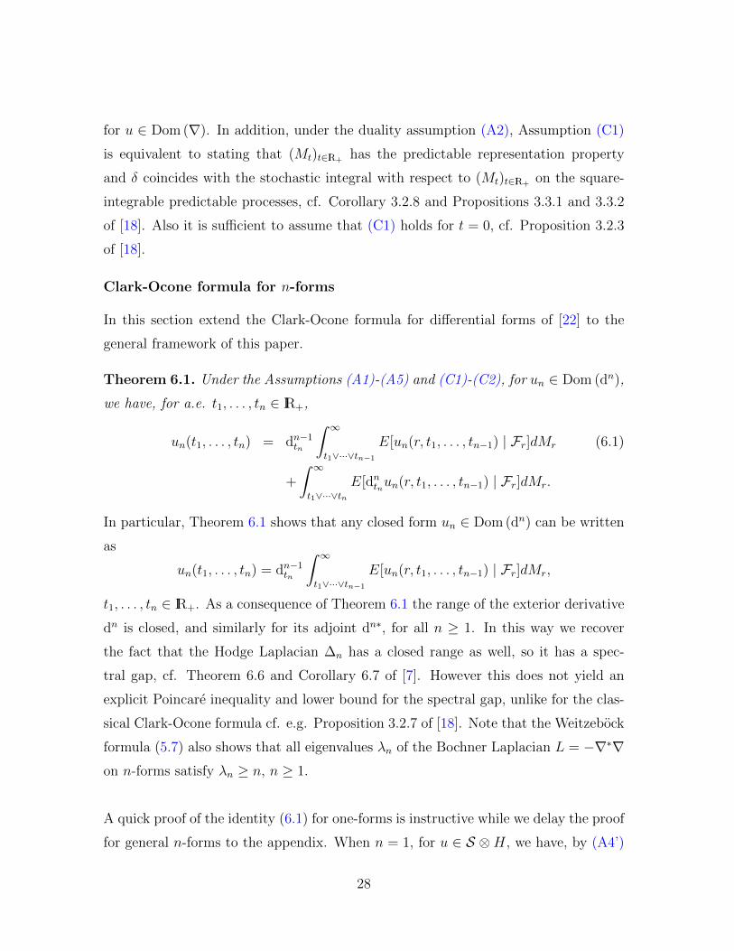
Theorem 6.1. Under the Assumptions (A1)-(A5) and (C1)-(C2), for un ∈ Dom (dn),

we have, for a.e. t1, . . . , tn ∈ IR+,

un(t1, . . . , tn) = dn−1tn

∫ ∞t1∨···∨tn−1

E[un(r, t1, . . . , tn−1) | Fr]dMr (6.1)

+

∫ ∞t1∨···∨tn

E[dntnun(r, t1, . . . , tn−1) | Fr]dMr.

In particular, Theorem 6.1 shows that any closed form un ∈ Dom (dn) can be written

as

un(t1, . . . , tn) = dn−1tn

∫ ∞t1∨···∨tn−1

E[un(r, t1, . . . , tn−1) | Fr]dMr,

t1, . . . , tn ∈ IR+. As a consequence of Theorem 6.1 the range of the exterior derivative

dn is closed, and similarly for its adjoint dn∗, for all n ≥ 1. In this way we recover

the fact that the Hodge Laplacian ∆n has a closed range as well, so it has a spec-

tral gap, cf. Theorem 6.6 and Corollary 6.7 of [7]. However this does not yield an

explicit Poincare inequality and lower bound for the spectral gap, unlike for the clas-

sical Clark-Ocone formula cf. e.g. Proposition 3.2.7 of [18]. Note that the Weitzebock

formula (5.7) also shows that all eigenvalues λn of the Bochner Laplacian L = −∇∗∇on n-forms satisfy λn ≥ n, n ≥ 1.

A quick proof of the identity (6.1) for one-forms is instructive while we delay the proof

for general n-forms to the appendix. When n = 1, for u ∈ S ⊗H, we have, by (A4’)

28

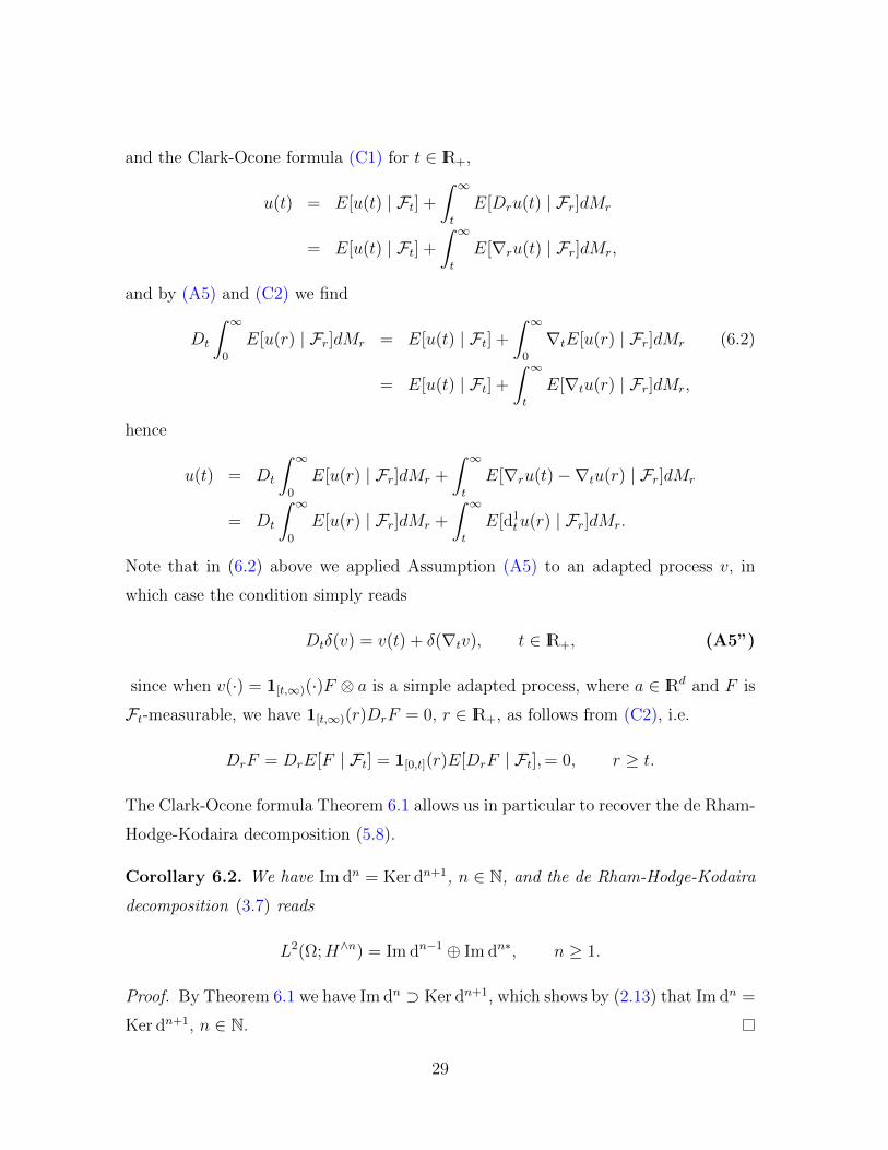
and the Clark-Ocone formula (C1) for t ∈ IR+,

u(t) = E[u(t) | Ft] +

∫ ∞t

E[Dru(t) | Fr]dMr

= E[u(t) | Ft] +

∫ ∞t

E[∇ru(t) | Fr]dMr,

and by (A5) and (C2) we find

Dt

∫ ∞0

E[u(r) | Fr]dMr = E[u(t) | Ft] +

∫ ∞0

∇tE[u(r) | Fr]dMr (6.2)

= E[u(t) | Ft] +

∫ ∞t

E[∇tu(r) | Fr]dMr,

hence

u(t) = Dt

∫ ∞0

E[u(r) | Fr]dMr +

∫ ∞t

E[∇ru(t)−∇tu(r) | Fr]dMr

= Dt

∫ ∞0

E[u(r) | Fr]dMr +

∫ ∞t

E[d1tu(r) | Fr]dMr.

Note that in (6.2) above we applied Assumption (A5) to an adapted process v, in

which case the condition simply reads

Dtδ(v) = v(t) + δ(∇tv), t ∈ IR+, (A5”)

since when v(·) = 1[t,∞)(·)F ⊗ a is a simple adapted process, where a ∈ IRd and F is

Ft-measurable, we have 1[t,∞)(r)DrF = 0, r ∈ IR+, as follows from (C2), i.e.

DrF = DrE[F | Ft] = 1[0,t](r)E[DrF | Ft],= 0, r ≥ t.

The Clark-Ocone formula Theorem 6.1 allows us in particular to recover the de Rham-

Hodge-Kodaira decomposition (5.8).

Corollary 6.2. We have Im dn = Ker dn+1, n ∈ N, and the de Rham-Hodge-Kodaira

decomposition (3.7) reads

L2(Ω;H∧n) = Im dn−1 ⊕ Im dn∗, n ≥ 1.

Proof. By Theorem 6.1 we have Im dn ⊃ Ker dn+1, which shows by (2.13) that Im dn =

Ker dn+1, n ∈ N.

29

As a consequence of Corollary 6.2, we also get the exactness of the sequence

Dom (dn)dn

−→ Im (dn) = Ker (dn+1)dn+1

−→ Im (dn+1), n ∈ N, (6.3)

as in Theorem 3.2 of [20]. By duality of (6.3) we also find by Corollary 6.2 that

Im d(n+1)∗ = Ker dn∗, n ∈ N,

and the following sequence is also exact:

Im (dn∗)dn∗←− Ker (dn∗) = Im (d(n+1)∗)

d(n+1)∗←− Dom (d(n+1)∗), n ∈ N.

Next, we consider some examples to which the above framework applies.

Commutative examples - chaos expansions

As written at the beginning of this section, we take X = IR+ in all cases due to the

need of a time scale in order to state the Clark-Ocone formula.

Example 3.1-a) - Normal martingales

As in Section 5 we have X = IR+ and ∇ = 0 on H, i.e. ∇ = D and Assumption (A4’)

is automatically satisfied. Let us check that Assumptions (C1) and (C2) are satisfied

in the framework of normal martingales that have the chaos representation property

(CRP).

(C1) Since the normal martingale (Mt)t∈IR+ has the chaos representation property,

the Clark-Ocone formula holds for any F ∈ Dom(D) ⊂ L2(Ω,F , P ) as

F = E[F ] +

∫ ∞0

E[DtF | Ft]dMt, (6.4)

cf. Proposition 4.2.3 of [18] for a proof via the chaos expansion of F .

(C2) This condition is satisfied from the definition (4.1) of D and e.g. Lemma 2.7.2

page 88 of [18] or Proposition 1.2.8 page 34 of [14] in the Wiener case.

30

Example 3.1-b) - Discrete-time chaos expansions

The Clark-Ocone formula (C1) holds in the discrete-time case as

F = E[F ] +∞∑k=0

E[DkF | Fk−1]Zk, (6.5)

cf. Proposition 1.7.1 of [18] and references therein, hence Assumption (C2) is also

satisfied here, as it is satisfied for normal martingales. However, Theorem 6.1 does

not hold here because (A5) is not satisfied.

Noncommutative example

Example 3.2) - Lie-Wiener path space (Example 1.3 continued)

(C1) On the classical Wiener space, when (u(t))t∈IR+ is square-integrable and adapted

to the Brownian filtration (Ft)t∈IR+ , δ(u) coincides with the Ito integral of

u ∈ L2(Ω;H) with respect to the underlying Brownian motion (Bt)t∈IR+ , i.e.

δ(u) =

∫ ∞0

u(t)dBt, (6.6)

and this shows that Assumption (C1) is satisfied, cf. e.g. Proposition 3.3.2 of

[18].

(C2) Assumption (C2) is satisfied here as in the case of normal martingales as in

e.g. Lemma 2.7.2 page 88 of [18], or for Brownian motion as in Proposition 1.2.8

page 34 of [14].

On the Lie-Wiener path space we note that we have the relation

〈DF, h〉H = 〈DF, h〉H + δ

(∫ ·0

ad(h(s))dsD·F

), F ∈ S, (6.7)

where D and δ denote here the gradient and divergence appearing in (4.4) on

the underlying standard Wiener space with Brownian motion (Bt)t∈IR+ in (4.8),

cf. e.g. Lemma 4.1 of [17] and references therein, or Corollary 5.2.1 of [16] for

the more general setting of Riemannian manifolds. Relation (6.7) shows that

E[DsF | Fr] = E[DsF | Fr], 0 ≤ r ≤ s, (6.8)

31

cf. also Relation (5.7.5) page 191 of [18] on Riemannian manifolds, hence (C1)

is satisfied for D because it holds for D as noted above.

Consequently, (C2) holds on the Lie-Wiener path space since we have

〈DE[F | Ft], h〉H = 〈DE[F | Ft], h〉H + δ

(∫ ·0

ad(h(s))dsD·E[F | Ft])

= 〈1[0,t](·)E[D·F | Ft], h〉H + δ

(∫ ·0

ad(h(s))ds1[0,t](·)E[D·F | Ft])

= 〈1[0,t](·)E[D·F | Ft], h〉H + E

[δ

(∫ ·0

1[0,t](s)ad(h(s))dsD·F

) ∣∣∣Ft]= 〈1[0,t](·)E[D·F | Ft], h〉H , t ∈ IR+.

Assumption (A4’) is also clearly satisfied by the definition (4.11) of ∇.

Hence Theorems 6.1 covers Theorems 3.1 of [22] on the Wiener space as well as its

extension to the path space using the diffeomorphism approach of [11].

Appendix

In this section we state the proofs of Proposition 3.1, Theorems 5.2 and 6.1, by

extension of the original arguments of [20], [10], [11], and [22] to our framework.

Proof of Proposition 3.1 (Duality relation). Assuming that un ∈ S ⊗H∧n and vn+1 ∈S ⊗H∧(n+1) have the form (2.6) and using the definition (2.4) of dn and the duality

assumption (A2) we have, using the antisymmetry of gn+1,

〈dntn+1(Ffn(t1, . . . , tn)), Ggn+1(t1, . . . , tn+1)〉L2(Ω,H∧(n+1))

=n+1∑j=1

(−1)j−1

(n+ 1)!〈∇tj(Ffn(t1, . . . , tj−1, tj+1, . . . , tn+1)), Ggn+1(t1, . . . , tn+1)〉L2(Ω,H⊗(n+1))

=n+1∑j=1

(−1)j−1

(n+ 1)!〈DtjFfn(t1, . . . , tj−1, tj+1, . . . , tn+1), Ggn+1(t1, . . . , tn+1)〉L2(Ω,H⊗(n+1))

32

+n+1∑j=1

(−1)j−1

(n+ 1)!〈F∇tjfn(t1, . . . , tj−1, tj+1, . . . , tn+1), Ggn+1(t1, . . . , tn+1)〉L2(Ω,H⊗(n+1))

=1

(n+ 1)!

n+1∑j=1

(−1)j−1〈Ffn(t1, . . . , tj−1, tj+1, . . . , tn+1),

δ(Ggn+1(t1, . . . , tj−1, ·, tj+1, . . . , tn+1))〉L2(Ω,H⊗n)

− 1

(n+ 1)!

n+1∑j=1

(−1)j−1〈Ffn(t1, . . . , tj−1, tj+1, . . . , tn+1),

G

∫ ∞0

Tr∇tgn+1(t1, . . . , tj−1, t, tj+1, . . . , tn+1)dt〉L2(Ω,H⊗n)

=1

(n+ 1)!

n+1∑j=1

〈Ffn(t1, . . . , tj−1, tj+1, . . . , tn+1),

δ(Ggn+1(·, t1, . . . , tj−1, tj+1, . . . , tn+1))〉L2(Ω,H⊗n)

− 1

(n+ 1)!

n+1∑j=1

〈Ffn(t1, . . . , tj−1, tj+1, . . . , tn+1),

G

∫ ∞0

Tr∇tgn+1(t, t1, . . . , tj−1, tj+1, . . . , tn+1)dt〉L2(Ω,H⊗n)

= 〈Ffn(t1, . . . , tn), dn∗(Ggn+1)(t1, . . . , tn)〉L2(Ω,H∧n),

where we applied the antisymmetry condition (A3) and the definition (3.2) of dn∗.

Proof of Lemma 5.1 (Intertwinning relation). When n = 1, by (A5) or (3.8) we have

d0x1

d0∗u1 = Dx1δ(u1)

= u1(x1) + δ(∇x1u1) + 〈DDx1F, f1〉H − 〈Dx1DF, f1〉H + 〈D·F,∇x1f1(·)〉H ,

for u1 = F ⊗ f1 ∈ S ⊗ H. Next, by the definition (2.4) of dn and (A5) or (3.8) we

have

dn−1tn δ(F ⊗ fn(·, x1, . . . , xn−1))

=n∑j=1

(−1)j−1∇xjδ(F ⊗ fn(·, x1, . . . , xj−1, xj+1, . . . , xn))

=n∑j=1

(−1)j−1F ⊗ fn(xj, x1, . . . , xj−1, xj+1, . . . , xn)

33

+n∑j=1

(−1)j−1δ(∇xj(F ⊗ fn(·, x1, . . . , xj−1, xj+1, . . . , xn)))

+n∑j=1

(−1)j−1〈D·DxjF −DxjD·F, fn(·, x1, . . . , xj−1, xj+1, . . . , xn)〉H

+n∑j=1

(−1)j−1〈D·F,∇(1)xjfn(·, x2, . . . , xj−1, xj+1, . . . , xn)〉H

= nF ⊗ fn(x1, . . . , xn)

+n∑j=1

δ(∇xj(F ⊗ fn(x1, . . . , xj−1, ·, xj+1, . . . , xn)))

+n∑j=1

∫X

〈DxF ⊗ fn(x1, . . . , xn),∇(j)xjgn(x1, . . . , xj−1, x, xj+1, . . . , xn)〉H∧nσ(dx).

where we applied (2.9). We conclude by the definition (3.2) of dn∗ which states that

d(n−1)∗(F ⊗ fn)(x1, . . . , xn−1) = δ(F ⊗ fn(·, x1, . . . , xn−1))

−F∫X

Tr∇xfn(x, x1, . . . , xn−1)σ(dx).

Proof of Theorem 5.2 (Weitzenbock identity). We will show that

‖d(n−1)∗un‖2L2(Ω,H⊗(n−1)) +

1

n+ 1‖dnun‖2

L2(Ω,H⊗(n+1))

= n‖un‖2L2(Ω,H⊗n) + ‖∇un‖2

L2(Ω,H⊗(n+1)),

for un ∈ S ⊗H∧n. By the intertwining relation of Lemma 5.1 combined with the use

of Assumption (B1) to reach (6.9) below, we have

〈dn−1d(n−1)∗un(x1, . . . , xn), gn(x1, . . . , xn)〉H∧n = nF 〈fn(x1, . . . , xn), gn(x1, . . . , xn)〉H∧n

+n∑j=1

〈δ((DxjF )⊗ fn(x1, . . . , xj−1, ·, xj+1, . . . , xn)), gn(x1, . . . , xn)〉H∧n

+n∑j=1

〈δ(F ⊗∇xjfn(x1, . . . , xj−1, ·, xj+1, . . . , xn), gn(x1, . . . , xn)〉H∧n

−n∑j=1

(−1)j−1 (6.9)

34

n∑l=2

⟨(DxjF )⊗

∫X

Tr∇(l)x fn(x, x1, . . . , xj−1, xj+1, . . . , xn)σ(dx), gn(x1, . . . , xn)

⟩H∧n

− F⟨∫

X

Tr∇xdn−1xn fn(x, x1, . . . , xn−1)σ(dx), gn(x1, . . . , xn)

⟩H∧n

(6.10)

+n∑j=1

∫X

〈(DxF )⊗ fn(x1, . . . , xn),∇(j)xjgn(x1, . . . , xj−1, x, xj+1, . . . , xn)〉H∧nσ(dx).

Hence, applying Assumption (A4) from (6.9)-(6.10) to (6.11)-(6.12), and Assump-

tion (A4) from (6.12) to (6.13), we find

〈dn−1xn d(n−1)∗un(·, x1, . . . , xn−1), vn(x1, . . . , xn)〉L2(Ω,H∧n)

= n〈un(x1, . . . , xn), vn(x1, . . . , xn)〉L2(Ω,H∧n)

+n∑j=1

〈δ((DxjF )⊗ fn(x1, . . . , xj−1, ·, xj+1, . . . , xn)), G⊗ gn(x1, . . . , xn)〉L2(Ω,H∧n)

+n∑j=1

〈δ(F ⊗∇xjfn(x1, . . . , xj−1, ·, xj+1, . . . , xn)), G⊗ gn(x1, . . . , xn)〉L2(Ω,H∧n)

+1

n

n∑j=1

(−1)n−jn−1∑l=1

∫X

∫X

〈(DyF )⊗ fn(x1, . . . , xj−1, x, xj+1, . . . , xn), (6.11)

G⊗∇(l)x gn(x1, . . . , xj−1, xj+1, . . . , xn, y)〉L2(Ω,H∧(n−1))σ(dx)σ(dy)

+1

n

n∑l=1

n∑j=1j 6=l

∫X

∫X

〈F ⊗∇(j)y fn(x1, . . . , xl−1, x, xl+1, . . . , xn), (6.12)

G⊗∇(l)x gn(x1, . . . , xj−1, y, xj+1, . . . , xn)〉L2(Ω,H∧(n−1))σ(dx)σ(dy)

+n∑l=1

(−1)n−j∫X

⟨(DyF )⊗ fn(x1, . . . , xn), G⊗∇(n)

xlgn(x1, . . . , xl−1, xl+1, . . . , xn, y)

⟩L2(Ω,H∧n)

σ(dy)

= n〈un(x1, . . . , xn), vn(x1, . . . , xn)〉L2(Ω,H∧n)

+1

n

n∑j=1

∫X

∫X

〈(DxF )⊗ fn(x1, . . . , xj−1, y, xj+1, . . . , xn),

(DyG)⊗ gn(x1, . . . , xj−1, x, xj+1, . . . , xn)〉L2(Ω,H∧(n−1))σ(dx)σ(dy)

+1

n

n∑j=1

∫X

∫X

〈F ⊗∇xfn(x1, . . . , xj−1, y, xj+1, . . . , xn),

(DyG)⊗ gn(x1, . . . , xj−1, x, xj+1, . . . , xn)〉L2(Ω,H∧(n−1))σ(dx)σ(dy)

35

+1

n

n∑j=1

(−1)n−jn∑l=1

∫X

∫X

〈(DyF )⊗ fn(x1, . . . , xj−1, x, xj+1, . . . , xn),

G⊗∇(l)x gn(x1, . . . , xj−1, xj+1, . . . , xn, y)〉L2(Ω,H∧(n−1))σ(dx)σ(dy)

+1

n

n∑j=1

n∑l=1

∫X

∫X

〈F ⊗∇(j)y fn(x1, . . . , xl−1, x, xl+1, . . . , xn), (6.13)

G⊗∇(l)x gn(x1, . . . , xj−1, y, xj+1, . . . , xn)〉L2(Ω,H∧(n−1))σ(dx)σ(dy)

= n〈un(x1, . . . , xn), vn(x1, . . . , xn)〉L2(Ω,H∧n)

+1

n

n∑l=1

∫X

∫X

〈(DxF )⊗ fn(x1, . . . , xl−1, y, xl+1, . . . , xn),

(DyG)⊗ gn(x1, . . . , xj−1, x, xj+1, . . . , xn)〉L2(Ω,H∧(n−1))σ(dx)σ(dy)

+1

n

n∑j=1

∫X

∫X

〈F ⊗∇xfn(x1, . . . , xj−1, y, xj+1, . . . , xn),

(DyG)⊗ gn(x1, . . . , xj−1, x, xj+1, . . . , xn)〉L2(Ω,H∧(n−1))σ(dx)σ(dy)

+1

n

n∑j=1

(−1)n−jn∑l=1

∫X

∫X

〈(DyF )⊗ fn(x1, . . . , xj−1, x, xj+1, . . . , xn),

G⊗∇(l)x gn(x1, . . . , xj−1, xj+1, . . . , xn, y)〉L2(Ω,H∧(n−1))σ(dx)σ(dy)

+1

n

n∑j=1

(−1)n−jn∑l=1

∫X

∫X

〈F ⊗∇(j)y fn(x1, . . . , xl−1, x, xl+1, . . . , xn),

G⊗∇(l)x gn(x1, . . . , xj−1, xj+1, . . . , xn, y)〉L2(Ω,H∧(n−1))σ(dx)σ(dy)

= n〈un(x1, . . . , xn), vn(x1, . . . , xn)〉L2(Ω,H∧n)

+1

n!

⟨(Dxn+1F )⊗ fn(x1, . . . , xn) + F ⊗∇xn+1fn(x1, . . . , xn),

n∑j=1

(−1)n−j(DxjG)⊗ gn(x1, . . . , xj−1, xj+1, . . . , xn, xn+1)

+n∑j=1

(−1)n−jn∑l=1

G⊗∇(l)xjgn(x1, . . . , xj−1, xj+1, . . . , xn, xn+1)

⟩L2(Ω,H⊗(n+1))

= n〈un(x1, . . . , xn), vn(x1, . . . , xn)〉L2(Ω,H∧n)

− (−1)n

n!

⟨(Dxn+1F )⊗ fn(x1, . . . , xn) + F ⊗∇xn+1fn(x1, . . . , xn),

n+1∑j=1

(−1)j−1(DxjG)⊗ gn(x1, . . . , xj−1, xj+1, . . . , xn+1)

36

+n+1∑j=1

(−1)j−1

n∑l=1

G⊗∇(l)xjgn(x1, . . . , xj−1, xj+1, . . . , xn+1)

⟩L2(Ω,H⊗(n+1))

+1

n!

⟨(Dxn+1F )⊗ fn(x1, . . . , xn) + F ⊗∇xn+1fn(x1, . . . , xn),

(Dxn+1G)⊗ gn(x1, . . . , xn) +G⊗n∑l=1

∇(l)xn+1

gn(x1, . . . , xn)

⟩L2(Ω,H⊗(n+1))

= n〈un(x1, . . . , xn), vn(x1, . . . , xn)〉L2(Ω,H∧n)

− (−1)n

n!

⟨(Dxn+1F )⊗ fn(x1, . . . , xn) + F ⊗∇xn+1fn(x1, . . . , xn),

n+1∑j=1

(−1)j−1(DxjG)⊗ gn(x1, . . . , xj−1, xj+1, . . . , xn+1)

+n+1∑j=1

(−1)j−1G⊗∇xjgn(x1, . . . , xj−1, xj+1, . . . , xn+1)

⟩L2(Ω,H⊗(n+1))

+1

n!

⟨(Dxn+1F )⊗ fn(x1, . . . , xn) + F ⊗∇xn+1fn(x1, . . . , xn),

(Dxn+1G)⊗ gn(x1, . . . , xn) +G⊗∇xn+1gn(x1, . . . , xn)⟩L2(Ω,H⊗(n+1))

= n〈un(x1, . . . , xn), vn(x1, . . . , xn)〉L2(Ω,H∧n)

− 1

(n+ 1)!

⟨n+1∑j=1

(−1)j−1(DxjF )⊗ fn(x1, . . . , xj−1, xj+1, . . . , xn+1)

+n+1∑j=1

(−1)j−1F ⊗∇xjfn(x1, . . . , xj−1, xj+1, . . . , xn+1),

n+1∑j=1

(−1)j−1(DxjG)⊗ gn(x1, . . . , xj−1, xj+1, . . . , xn+1)

+n+1∑j=1

(−1)j−1G⊗∇xjgn(x1, . . . , xj−1, xj+1, . . . , xn+1)

⟩L2(Ω,H⊗(n+1))

+1

n!

⟨(Dxn+1F )⊗ fn(x1, . . . , xn) + F ⊗∇xn+1fn(x1, . . . , xn),

(Dxn+1G)⊗ gn(x1, . . . , xn) +G⊗∇xn+1gn(x1, . . . , xn)⟩L2(Ω,H⊗(n+1))

= n〈un(x1, . . . , xn), vn(x1, . . . , xn)〉L2(Ω,H∧n) − 〈dnun, dnvn〉L2(Ω,H∧(n+1))

+1

n!〈∇xn+1un(x1, . . . , xn),∇xn+1vn(x1, . . . , xn)〉L2(Ω,H∧(n+1)),

37

where we used (A4). Hence we have

〈d(n−1)∗un, d(n−1)∗vn〉L2(Ω,H∧n) + 〈dnun, dnvn〉L2(Ω,H∧(n+1))

= n〈un, vn〉L2(Ω,H∧n) +1

n!〈∇un,∇vn〉L2(Ω,H⊗(n+1)),

i.e.

〈d(n−1)∗un, d(n−1)∗vn〉L2(Ω,H⊗n) +

1

n+ 1〈dnun, dnvn〉L2(Ω,H⊗(n+1))

= n〈un, vn〉L2(Ω,H⊗n) + 〈∇un,∇vn〉L2(Ω,H⊗(n+1)),

and applying the duality

〈∇un,∇vn〉L2(Ω,H⊗(n+1)) = 〈∇∗∇un, vn〉L2(Ω,H∧n), un, vn ∈ S ⊗H∧n,

we get

dn−1d(n−1)∗ + dn∗dn = nIH∧n +∇∗∇.

Proof of Theorem 6.1 (Clark-Ocone formula).

By the Clark-Ocone formula (C1) and Assumption (A4’) we have

un(t1, . . . , tn) = E[un(t1, . . . , tn) | Ft1∨···∨tn ] +

∫ ∞t1∨···∨tn

E[Drun(t1, . . . , tn) | Fr]dMr

= E[un(t1, . . . , tn) | Ft1∨···∨tn ] +

∫ ∞t1∨···∨tn

E[∇run(t1, . . . , tn) | Fr]dMr, (6.14)

t1, . . . , tn ∈ IR+. Next, by the definition (2.4) of dn and (3.8) applied to adapted

processes we have

dn−1tn

∫ ∞t1∨···∨tn−1

E[un(r, t1, . . . , tn−1) | Fr]dMr

=n∑j=1

(−1)j−1∇tj

∫ ∞t1∨···∨tj−1∨tj+1∨···∨tn

E[un(r, t1, . . . , tj−1, tj+1, . . . , tn) | Fr]dMr

=n∑j=1

(−1)j−11[t1∨···∨tn,∞)(tj)E[un(tj, t1, . . . , tj−1, tj+1, . . . , tn) | Ftj ]

+n∑j=1

(−1)j−1

∫ ∞t1∨···∨tj−1∨tj+1···∨tn

∇tjE[un(tn+1, t1, . . . , tj−1, tj+1, . . . , tn) | Ftn+1 ]dMtn+1

38

=n∑j=1

1[t1∨···∨tn,∞)(tj)E[un(t1, . . . , tn) | Ftj ]

+n∑j=1

(−1)j−1

∫ ∞t1∨···∨tj−1∨tj+1···∨tn

∇tjE[un(tn+1, t1, . . . , tj−1, tj+1, . . . , tn) | Ftn+1 ]dMtn+1

= E[un(t1, . . . , tn) | Ft1∨···∨tn ]

+n∑j=1

(−1)j−1

∫ ∞t1∨···∨tn

E[∇tjun(tn+1, t1, . . . , tj−1, tj+1, . . . , tn) | Ftn+1 ]dMtn+1 , (6.15)

where on the last line we used the fact that by (A4),∇tjun(tn+1, t1, . . . , tj−1, tj+1, . . . , tn)

vanishes when t1 ∨ · · · ∨ tj−1 ∨ tj+1 · · · ∨ tn < tn+1 < tj, hence by taking the difference

of (6.14) and (6.15) we find

un(t1, . . . , tn) = dn−1tn

∫ ∞t1∨···∨tn−1

E[un(r, t1, . . . , tn−1) | Fr]dMr

−n∑j=1

(−1)j−1

∫ ∞t1∨···∨tn

E[∇tjun(t1, . . . , tj−1, tj+1, . . . , tn+1) | Ftn+1 ]dMtn+1

+

∫ ∞t1∨···∨tn

E[∇run(t1, . . . , tn) | Fr]dMr

= dn−1tn

∫ ∞t1∨···∨tn−1

E[un(r, t1, . . . , tn−1) | Fr]dMr

+

∫ ∞t1∨···∨tn

E[dntn+1un(t1, . . . , tn) | Ftn+1 ]dMtn+1 ,

t1, . . . , tn ∈ IR+.

References

[1] S. Aida. Vanishing of one-dimensional L2-cohomologies of loop groups. J. Funct. Anal.,261(8):2164–2213, 2011.

[2] S. Albeverio, A. Daletskii, and E. Lytvynov. De Rham cohomology of configuration spaces withPoisson measure. J. Funct. Anal., 185(1):240–273, 2001.

[3] S. Albeverio, A. Daletskii, and E. Lytvynov. Laplace operators on differential forms over con-figuration spaces. J. Geom. Phys., 37(1-2):15–46, 2001.

[4] L. Bartholdi, T. Schick, N. Smale, and S. Smale. Hodge theory on metric spaces. Found.Comput. Math., 12(1):1–48, 2012.

[5] J.M.C. Clark. The representation of functionals of Brownian motion by stochastic integrals.Annals of Mathematical Statistics, 41:1281–1295, 1970.

39

[6] A.B. Cruzeiro and P. Malliavin. Renormalized differential geometry on path space: Structuralequation, curvature. J. Funct. Anal., 139:119–181, 1996.

[7] K. D. Elworthy and Y. Yang. The vanishing of L2 harmonic one-forms on based path spaces.J. Funct. Anal., 264(5):1168–1196, 2013.

[8] M. Emery. On the Azema martingales. In Seminaire de Probabilites XXIII, volume 1372 ofLecture Notes in Mathematics, pages 66–87. Springer Verlag, 1990.

[9] S. Fang and J. Franchi. Flatness of Riemannian structure over the path group and energyidentity for stochastic integrals. C. R. Acad. Sci. Paris Ser. I Math., 321(10):1371–1376, 1995.

[10] S. Fang and J. Franchi. De Rham-Hodge-Kodaira operator on loop groups. J. Funct. Anal.,148(2):391–407, 1997.

[11] S. Fang and J. Franchi. A differentiable isomorphism between Wiener space and path group. InSeminaire de Probabilites, XXXI, volume 1655 of Lecture Notes in Math., pages 54–61. Springer,Berlin, 1997.

[12] T. Kazumi and I. Shigekawa. Differential calculus on a submanifold of an abstract Wiener space,ii: Weitzenbock formula. In Walter de Gruyter & Co., editor, Procedings of the conference onDirichlet forms and stochastic processes, pages 235–251, 1993.

[13] S. Kobayashi and K. Nomizu. Foundations of differential geometry. Vol I. Interscience Pub-lishers, a division of John Wiley & Sons, New York-London, 1963.

[14] D. Nualart. The Malliavin calculus and related topics. Probability and its Applications. Springer-Verlag, Berlin, second edition, 2006.

[15] D. Ocone. Malliavin’s calculus and stochastic integral representations of functionals of diffusionprocesses. Stochastics, 12(3-4):161–185, 1984.

[16] J.J. Prat and N. Privault. Explicit stochastic analysis of Brownian motion and point measureson Riemannian manifolds. J. Funct. Anal., 167:201–242, 1999.

[17] N. Privault. Quantum stochastic calculus applied to path spaces over Lie groups. In Proceedingsof the International Conference on Stochastic Analysis and Applications, pages 85–94. KluwerAcad. Publ., Dordrecht, 2004.

[18] N. Privault. Stochastic analysis in discrete and continuous settings with normal martingales,volume 1982 of Lecture Notes in Mathematics. Springer-Verlag, Berlin, 2009.

[19] N. Privault. De Rham-Hodge decomposition and vanishing of harmonic forms by derivationoperators on the Poisson space. Preprint, 34 pages, 2015.

[20] I. Shigekawa. de Rham-Hodge-Kodaira’s decomposition on an abstract Wiener space. J. Math.Kyoto Univ., 26(2):191–202, 1986.

[21] D. Surgailis. On multiple Poisson stochastic integrals and associated Markov semi-groups.Probability and Mathematical Statistics, 3:217–239, 1984.

[22] Y. Yang. Generalised Clark-Ocone formulae for differential forms. Commun. Stoch. Anal.,6(2):323–337, 2012.

40