Atmospheric Thermodynamics Atmospheric Composition What is the composition of the Earth’s atmosphere? Gaseous Constituents of the Earth’s atmosphere (dry air)

Constituent

Molecular Weight

Fractional Concentration by Volume of Dry Air

Nitrogen (N2) 28.013 78.08% Oxygen (O2) 32.000 20.95% Argon (Ar) 39.95 0.93%

Carbon Dioxide (CO2) 44.01 380 ppm Neon (Ne) 20.18 18 ppm

Helium (He) 4.00 5 ppm Methane (CH4) 16.04 1.75 ppm

Krypton (Kr) 83.80 1 ppm Hydrogen (H2) 2.02 0.5 ppm

Nitrous oxide (N2O) 44.013 0.3 ppm Ozone (O3) 48.00 0-0.1 ppm

Water vapor is present in the atmosphere in varying concentrations from 0 to 5%. Aerosols – solid and liquid material suspended in the air What are some examples of aerosols? The particles that make up clouds (ice crystals, rain drops, etc.) are also considered aerosols, but are more typically referred to as hydrometeors. We will consider the atmosphere to be a mixture of two ideal gases, dry air and water vapor, called moist air.

Gas Laws Equation of state – an equation that relates properties of state (pressure, volume, and temperature) to one another Ideal gas equation – the equation of state for gases

p – pressure (Pa) V – volume (m3) m – mass (kg) R – gas constant (value depends on gas) (J kg-1 K-1) T – absolute temperature (K) This can be rewritten as:

r - density (kg m-3) or as:

a - specific volume (volume occupied by 1 kg of gas) (m3 kg-1) Boyle’s Law – for a fixed mass of gas at constant temperature Charles’ Laws: For a fixed mass of gas at constant pressure For a fixed mass of gas at constant volume

€

pV = mRT

€

p =mVRT

p = ρRT

€

p Vm

= RT

pα = RT

€

V ∝1 p

€

V ∝T

€

p∝T

Mole (mol) – gram-molecular weight of a substance The mass of 1 mol of a substance is equal to the molecular weight of the substance in grams.

n – number of moles m – mass of substance (g) M – molecular weight (g mol-1) Avogadro’s number (NA) – number of molecules in 1 mol of any substance NA = 6.022x1023 mol-1 Avogadro’s hypothesis – gases containing the same number of molecules (or moles) occupy the same volume at the same temperature and pressure Using the ideal gas law and the definition of a mole gives:

Using this form of the ideal gas law with Avogadro’s hypothesis indicates that MR is constant for all gases. This constant is known as the universal gas constant (R*).

= 8.3145 J K-1 mol-1 With the universal gas constant the ideal gas law becomes:

€

n =mM

€

pV = nMRT

€

R* = MR

€

pV = nR*T

Application of the ideal gas law to dry air

or pd – pressure exerted by dry air rd – density of dry air Rd – gas constant for dry air ad – specific volume for dry air

, where

Md – apparent molecular weight of dry air (=28.97 g mol-1)

mi – mass of ith constituent of dry air ni – number of moles of ith constituent of dry air Example: Calculate the gas constant for dry air Example: Calculate the density of air at SEEC. Why is the density calculated here not exactly correct?

€

pd = ρd RdT

€

pdαd = RdT

€

Rd =R*

Md

€

Md =md

n=

mii∑mi

Mii∑

=

mii∑

nii∑

Application of the ideal gas law to individual components of air Each gas that makes up the atmosphere obeys the ideal gas law:

For water vapor the ideal gas law is:

or e – pressure exerted by water vapor (vapor pressure) rv – density of water vapor av – specific volume of water vapor Rv – gas constant for water vapor Example: Calculate the gas constant for water vapor Dalton’s law of partial pressure – the total pressure exerted by a mixture of gases that do not interact chemically is equal to the sum of the partial pressure of the gases

Partial pressure – pressure exerted by a gas at the same temperature as a mixture of gases if it alone occupied all of the volume that the mixture occupies Example: The pressure in a hurricane is observed to be 950 mb. At this time the temperature is 88 deg F and the vapor pressure is 25 mb. Determine the density of dry air alone and the density of water vapor alone.

€

pi = ρi RiT

€

e = ρv RvT

€

eαv = RvT

p = pii∑ = T ρi

i∑ Ri

Virtual Temperature How does the gas constant vary as the molecular weight of the gas being considered changes? The molecular weight of dry air is greater than the molecular weight of moist air (i.e. one mole of dry air has a larger mass than one mole of moist air) What does this imply about the gas constant for moist air compared to dry air? For dry and moist air at the same temperature and pressure which will have the smaller density? As the amount of moisture in the air changes the molecular weight of the moist air will also change causing the gas constant for the moist air to vary. The density of moist air is given by:

, where

r - density of moist air md - mass of dry air mv - mass of moist air V - volume

- density that mass md of dry air would have if it occupied volume V - density that mass mv of water vapor would have if it occupied volume V

and can be considered partial densities (analogous to partial

pressures) Using the ideal gas law the partial pressure of dry air (pd) and water vapor (e) can be calculated as:

and

€

ρ =md + mv

V= ρd

' + ρv'

€

ρd'

€

ρv'

€

ρd'

€

ρv'

€

pd = ρd' RdT

€

e = ρv' RvT

From Dalton’s law the total pressure exerted by the moist air is:

Rewriting in terms of the density of moist air (r) gives:

where

This equation can be rewritten in terms of the virtual temperature (Tv) as:

or

where

The virtual temperature is the temperature dry air would need to have if it were to have the same density as a sample of moist air at the same pressure How does the magnitude of Tv compare to the magnitude of T?

€

p = pd + e

= ρd' RdT + ρv

' RvT

€

ρ =pdRdT

+eRvT

=p − eRdT

+eRvT

=pRdT

1− ep1− Rd

Rv

$

% &

'

( )

*

+ ,

-

. /

=pRdT

1− ep1−ε( )

*

+ ,

-

. /

€

ε =RdRv

=Mw

Md= 0.622

€

ρ =p

RdTv

€

p = ρRdTv

€

Tv ≡T

1− ep1−ε( )

Example: The pressure in a hurricane is observed to be 950 mb. At this time the temperature is 88 deg F and the vapor pressure is 25 mb. Calculate the virtual temperature in the hurricane. How does the observed temperature compare to the virtual temperature? Calculate the density of dry air, with a pressure of 950 mb, and the actual density of the moist air in the hurricane. Which density is greater?

The Hydrostatic Equation At any point in the atmosphere the atmospheric pressure is equal to the weight per unit area of all of the air lying above that point. Therefore, atmospheric pressure decreases with increasing height in the atmosphere. This results in an upward directed pressure gradient force. For any mass of atmosphere there is downward directed gravitational force.

Hydrostatic balance - the upward directed pressure gradient force is exactly balanced by the downward directed gravitational force.

What would happen if the vertical pressure gradient force and gravitational force were not in balance? Derivation of the hydrostatic equation Consider a thin slab of the atmosphere, with depth dz and unit cross-sectional area (1 m2). If the density of this air is r then the mass of the slab is given by: m = rdz(1 m2) The gravitational force acting on this slab of air is: mg = grdz(1 m2) where g is the acceleration due to gravity (=9.81 m s-2)

The change in pressure between height z and z+dz is dp. What is the sign of dp? The upward directed pressure gradient force, due to the decrease of pressure with height, is given by -dp For hydrostatic balance: -dp = grdz and in the limit as dz ® 0

, which is the hydrostatic equation

This can also be written as and integrated from height z to the top of the atmosphere to give:

What is the pressure at a height of z = ∞? This is the mathematical expression that indicates that the pressure at any height in the atmosphere is equal to the weight per unit area of all of the overlying air.

∂ p∂z

= −ρg

€

∂p = −ρg∂z

€

− ∂pp (z )

p (∞)

∫ = gρ∂zz

∞

∫

p(z) = gρ∂zz

∞

∫

Geopotential Geopotential (F) – the work that must be done against the Earth’s gravitational field to raise a mass of 1 kg from sea level to a height z (i.e. the gravitational potential per unit mass) The force acting on a unit mass of the atmosphere at height z is g. The work required to raise this mass from z to z+dz is gdz and 𝑑Φ ≡ 𝑔𝑑𝑧 What are the units of geopotential? Integrating this equation gives the geopotential (F(z)) at height z:

By convention F(0) = 0 m2 s-2 Since the equation for F(z) is an integral of an exact differential the value of F(z) does not depend on the path taken to get to height z. Geopotential height (Z)

where g0 is the globally averaged acceleration due to gravity at the Earth’s surface (=9.81 m s-2).

€

Φ(z) = gdz0

z

∫

€

Z ≡ Φ(z)g0

=1g0

gdz0

z

∫

Since g ≈ g0 in the lower atmosphere Z ≈ z, as shown below. z (km) Z (km) g (m s-2)

0 0 9.81 1 1.00 9.80

10 9.99 9.77 100 98.47 9.50 500 463.6 8.43

Thickness Using the ideal gas law we can eliminate r in the hydrostatic equation:

Using the definition of dF gives

Integrating this between geopotentials F1 and F2 gives:

Dividing by g0 gives

The difference Z2 – Z1 is referred to as the thickness between pressure levels p1 and p2.

€

∂p∂z

= −ρg = −pgRdTv

€

dΦ = gdz = −RdTvdpp

€

dΦΦ1

Φ2

∫ = − RdTvdppp1

p2

∫

Φ2 −Φ1 = −Rd Tvdppp1

p2

∫

€

Z2 − Z1 =Rdg0

Tvdppp2

p1

∫

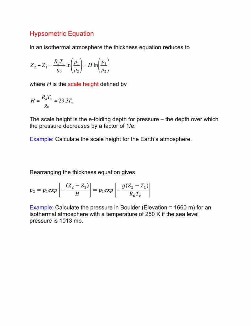
Hypsometric Equation In an isothermal atmosphere the thickness equation reduces to

where H is the scale height defined by

The scale height is the e-folding depth for pressure – the depth over which the pressure decreases by a factor of 1/e. Example: Calculate the scale height for the Earth’s atmosphere. Rearranging the thickness equation gives

𝑝' = 𝑝)𝑒𝑥𝑝 ,−(𝑍' − 𝑍))

𝐻2 = 𝑝)𝑒𝑥𝑝 ,−

𝑔(𝑍' − 𝑍))𝑅4𝑇6

2

Example: Calculate the pressure in Boulder (Elevation = 1660 m) for an isothermal atmosphere with a temperature of 250 K if the sea level pressure is 1013 mb.

€

Z2 − Z1 =RdTvg0

ln p1p2

#

$ %

&

' ( = H ln

p1p2

#

$ %

&

' (

€

H =RdTvg0

= 29.3Tv

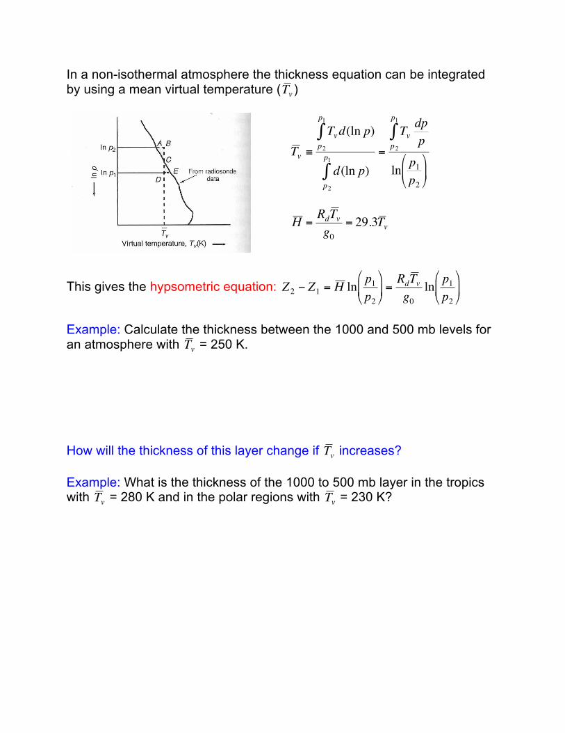
In a non-isothermal atmosphere the thickness equation can be integrated by using a mean virtual temperature ( )

This gives the hypsometric equation:

Example: Calculate the thickness between the 1000 and 500 mb levels for an atmosphere with = 250 K. How will the thickness of this layer change if increases? Example: What is the thickness of the 1000 to 500 mb layer in the tropics with = 280 K and in the polar regions with = 230 K?

€

T v

€

T v ≡Tv d(ln p)

p2

p1

∫

d(ln p)p2

p1

∫=

Tvdppp2

p1

∫

ln p1p2

$

% &

'

( )

€

H = RdT vg0

= 29.3T v

€

Z2 − Z1 = H ln p1p2

#

$ %

&

' ( =

RdT vg0

ln p1p2

#

$ %

&

' (

€

T v

€

T v

€

T v

€

T v

Upper Level Weather Maps Since pressure always decreases with height in the atmosphere, and above any given spot on the earth each height has a unique pressure, we can use pressure as a vertical coordinate. Weather data on upper level weather maps are plotted on constant pressure surfaces rather than constant height surfaces (such as a sea level pressure map). Pressure surface – an imaginary surface where the pressure has a constant value One of the key properties meteorologists are interested in when looking at a constant pressure map is the geopotential height of the constant pressure surface. Consider a layer of the atmosphere between sea level and the 700 mb constant pressure surface:

The thickness of this layer, and thus geopotential height of the 700 mb surface, varies with the temperature of the column of air below 700 mb surface. Lower heights correspond to a colder column temperature. Therefore, we expect (and do) find lower constant pressure heights near the poles and higher heights in the tropics.

Commonly Used Constant Pressure Maps Pressure

Level Approximate Altitude (ft)

Approximate Altitude (km)

850 mb About 5,000 ft About 1.5 km 700 mb About 10,000 ft About 3.0 km 500 mb About 18,000 ft About 5.5 km 300 mb About 30,000 ft About 9.0 km 250 mb About 35,000 ft About 10.5 km 200 mb About 39,000 ft About 12.0 km

Upper Air Station Model

What are the differences between surface and upper air station models? Some upper air weather map terms: Trough – region of low heights on a constant pressure map Ridge – region of high heights on a constant pressure map Shortwave – a small ripple in the height field Longwave – a large ripple in the height field

Example: Real-time constant pressure weather maps How does the height of the 500 mb surface vary from south to north? What is the relationship between winds and height contours on an upper level constant pressure map? Does this relationship vary between the Northern and Southern hemispheres? What wind direction should we expect to find in the mid-latitudes if lower constant pressure surface heights are found near the poles and higher heights are found in the tropics? Reduction of Pressure to Sea Level Since pressure decreases with altitude, the pressure measured by a weather station in the mountains will be less than the pressure measured by a weather station at sea level. Because meteorologists are interested in horizontal changes in pressure, the pressures measured at weather stations across the Earth need to be interpolated to a common height, which is typically sea level. This interpolation can be done by solving the hypsometric equation for p1, the pressure at sea level, and noting that Z1 = 0 m:

In this equation Z2 is the elevation of the weather station and p2 is the pressure measured by this weather station. Example: Calculate the sea level pressure based on the current weather observation from the ATOC weather station

€

Z2 − Z1 =RdT vg0

ln p1p2

#

$ %

&

' (

Z2 =RdT vg0

ln p1p2

#

$ %

&

' (

p1 = p2 expg0Z2

RdT v

#

$ %

&

' (