Page | 1

What Determines TSR – Executive Summary (Download the full report at www.evaDimensions.com/EVA2TSR/report)

By Bennett Stewart CEO, EVA Dimensions LLC, Author of Best-Practice EVA Copyright © 2013 by EVA Dimensions LLC. All rights reserved.

Total shareholder return, always an important measure, has achieved much greater prominence

over the past few years. One reason is that Institutional Shareholder Services (ISS), the largest proxy

adviser, has announced that it is using TSR, and TSR alone, to test the adequacy of links between

incentive pay and company performance. Boards are understandably concerned, especially in the new

era of say-on-pay proxy voting, and compensation committees are scrambling to understand the

implications for pay plans. The most important implication, explained in detail below, is that companies

ought to scrap most existing plans and opt for ones that base bonus awards on economic profit or, as I

call it, EVA, standing for economic value added. EVA is the performance measure that best ranks

companies by the TSRs they generate and it is also one that managers can actually manage.

The emphasis that ISS and others are putting on TSR makes sense. TSR, after all, is the rate of

return investors receive, measured as dividend yield plus the percent change in share price over a

holding period. It is the only performance that shareholders can take to the bank, and the ultimate

gauge of the success or failure of their investment. Maximizing TSR should be a key goal of every

company, especially when viewed over longer horizons and relative to peer companies, which is the

perspective ISS is taking as well.

The TSR test, however, creates serious problems for compensation committees. For one, TSR

measures the return but is mute about how that return was generated—or how to go about increasing

it. It also cannot be measured for individual business lines or business decisions. It is simply too

abstract and too far removed from actual decision-making to motivate managers in ways that will

actually improve the return. Nearly everyone recognizes this, including ISS, which advises companies to

base incentives on short- and long-term business goals and not on TSR. What’s needed is to understand

the business success factors that drive TSR, and to pay for them and use them in managing the business.

This leads to the second, greater problem. Every conventional metric—earnings, earnings

growth, EPS, the assorted rate-of-return measures, cash flow—can produce a performance “answer”

that is the opposite of what’s really happening. Each one can “improve” when true economic

performance and company value and TSR are deteriorating, and can look bad when a company’s

fortunes actually have risen. Each one tells half-truths or outright untruths, but never the whole truth.

A company’s reported earnings, for example, increase whenever the rate of return it earns on

incremental investment exceeds the after-tax cost of the funds borrowed to finance the investment,

which these days might be as paltry as just a few percentage points. Stock prices, however, increase

Page | 2

only if the return covers the full weighted average cost of capital. Put another way, using earnings to

judge corporate performance is like judging a basketball player by the number of points scored. That

gives each player the incentive to take as many shots as possible in the hope of scoring points even

when others have a better shot at the basket1.

Return measures are also flawed, but in the opposite direction. Judging corporate performance

with a return measure is like judging a basketball player by shooting percentage. The incentive is to take

a sure layup and then stop shooting. ROI-focused firms behave like that. They neglect genuinely

profitable expansion opportunities that happen to generate returns lower than their existing ROI or

lower than an arbitrary return target that top management has established. This has led to some of the

biggest blunders in business history. IBM delayed entering the desktop PC business throughout the

1970s in order to avoid diluting the 25% ROI it was earning in its mainframe business—and handed

fortunes to West Coast startups in the process. In a more recent example August Busch rejected global

expansion at Anheuser Busch because it would not match the frothy returns and margins he was

earnings in his domestic beer business—which ultimately made the company vulnerable to a hostile

takeover. It is little wonder Harvard Professor Clay Christensen has blamed a fixation on maintaining

high margins and returns with the “Innovator’s Dilemma,” which is the tendency of established

companies to cede leadership to upstart rivals2.

Compensation consultants generally understand this and are in broad agreement that no

conventional financial measure provides a truly reliable score on corporate performance or a

trustworthy link to TSR. As a result, most pay advisers counsel clients to use at least two or three

metrics in ways that appropriately balance growth and profitability. ISS, too, acknowledges that no

single standard exists to measure corporate performance and manage a business in a way that directly

contributes to improving TSR, and so it advises companies that “key metrics may vary considerably from

industry to industry and from company to company depending on their particular business strategy at

any given time.”

So how can directors—or anyone, for that matter—know which metrics to choose and how to

weight them? How does a comp committee balance an increase in earnings with a decline in ROI, for

instance, when the goal is to propel the firm’s TSR? Most important, how does this metric soup of

conflicting measures provide managers with the practical information and insights they and their teams

need to make the best decisions?

Contrary to popular opinion, there is an answer. The solution lies in using EVA. It is the one and

only financial metric with a direct, provable link to TSR, as I will show. EVA measures profit according to

economic principles and for the purpose of managing a business and maximizing value, and not by

following accounting conventions. The biggest difference is that EVA measures profit after deducting a

charge for the full weighted-average cost of all the capital invested in a firm’s business assets, which

includes setting aside a minimum competitive return for the shareowners. If a firm’s net operating

profit after taxes, or NOPAT, is $150, and if it has $1,000 invested in net business assets with a 10%

1 For a detailed critique of earnings growth, consult “Let’s Abandon Earnings Per Share,” available from the author.

2 For a detailed critique of ROI, consult “Stop Using ROI,” available from the author.

Page | 3

blended cost of capital, for a capital charge of $100, then its EVA is $50, the remainder. Put simply, EVA

measures quality earnings after setting aside a priority return for the owners (and in practice after

eliminating other accounting distortions that make no business or economic sense3). An increase in EVA

profit is thus a surer indication than any other that a company has truly made progress and increased its

value through some combination of cutting costs, managing its assets and turning them faster, and

profitably growing its business. No other measure or combination of measures captures the total

essence of performance so succinctly and so accurately.

This is not just an assertion or a debatable point. More EVA will always produce a higher TSR

than less EVA for any company. I will demonstrate this by first explaining the theoretical link between

EVA and TSR. I will show, through logic and with simple formulas, that managing for higher EVA is, by

definition, managing for a higher TSR. Then I will present empirical evidence that EVA does, in fact,

explain differences in TSR better and more completely than any other financial metric.

The underlying reason is that EVA has a wholly predictable, actually mathematical, link with

creating value. The link is net present value. As modern financial theory holds, the intrinsic value of

every company is the net present value, or NPV, of the cash flows it will generate in the future. That is

well known and generally acknowledged to be true. What is not so well known, but crucial, is that for

any given set of assumptions about future operations, the present value of the forecasted EVA is always

exactly the same as the net present value of forecasted cash flows. That is because EVA sets aside the

profit that must be earned in each period to recover the value of the capital that has been or will be

invested. As a result, EVA always discounts to the value added to the invested capital, which is the same

thing as the net present value.

If an investment decision or business plan shows that EVA will run around zero (in other words,

that it will just break even in an economic sense of covering the full opportunity cost of all resources,

including a competitive return on the capital) then the net present value of cash flows generated by that

business plan or investment will also be zero, by definition. Simply put, no EVA is no NPV. The only way

that value is created—that investors will realize a premium value above the capital they’ve put or left in

the business—is if a positive EVA profit is earned. And the more EVA earned, and the faster it grows,

and the longer and surer it endures, the greater will be the firm’s franchise value and its overall net

present value.

The implications of this are enormous. It means that EVA is the very best performance goal for

maximizing TSR. Because managing for the highest possible EVA is the same thing as managing for the

3 Other distortions EVA eliminates include: removing excess cash to focus on business profits; treating leased assets as if they are owned;

reversing impairment charges by taking them out of earnings and putting them back into balance sheet capital (no mulligans are allowed to artificially increase EVA in subsequent periods); similarly, adding restructuring charges back to earnings and back to balance sheet capital, subject to the capital charge (the incentive is for managers to fail fast—no charge stands in their way—and to fail well—to invest cash in streamlining the business only if it will cover the cost of capital); writing off R&D and brand-building advertising outlays over time, like 3-5 years, and subjecting them to the cost of capital interest charge on the un-amortized balance (which deters managers from cutting the spending to make a short term earnings goal and encourages them to increase it if the investment is strategically promising); smoothing tax gyrations and crediting EVA for the cost of capital saved by deferring taxes; swapping service cost for the reported pension cost and correctly accounting for the cost of closing a funding gap; and holding back a portion of the capital invested in strategic decisions, like acquisitions, and metering it back into capital over time, with interest. The adjustments make EVA a surer, sooner measure of the value-added period by period, but not without some added complexity. In practice, each company must choose to track the 3-5 most material and applicable adjustments.

Page | 4

highest NPV, then maximizing EVA has to produce the highest TSR over time. Cash dividends and cash-

equivalent share-price changes are simply the messengers. They just transmit the return that is in fact

determined by the firm’s EVA. That’s the idea in a nutshell, but as I said, a formal proof is coming, and it

requires the use of two other variables, TIR and MVA, which bear explanation.

TIR stands for total investor return. It is the return a company generates on behalf of all

investors—its lenders and shareholders combined. It’s the return you’d get if you bought all the stock

and bonds and held all of the liabilities of the company (except trade credit). It’s the return that flows

out of the business, and as it happens, it is the underlying source of TSR. The return that a firm provides

to its shareholders is always just a leveraged version of the return it earns in its business.

TIR is computed similarly to TSR, as a cash yield and capital gain, but for the company as a

whole. To be specific, it is the return generated by the company’s “free” cash flow plus the change in

the company’s overall market value over the period, divided by the market value of the firm’s debt and

equity at the beginning of the period4.

Free cash flow, or FCF for short, is the net cash generated or required by the firm’s business

activities, and as such, it is also equal to the cash sum that can be paid out to all the investors—to the

lenders and shareholders combined—or that must be raised from them if it is negative. It is computed

by taking the NOPAT the firm generates in the period and deducting the period to period change in the

amount of balance sheet capital tied up in business assets. What’s left over is its free cash flow available

to distribute or that must be financed5.

A cautionary note—the role of free cash flow in the TIR calculation is not what it may seem. If a

company steps up investment spending, its free cash flow in the period goes down, and may even turn

negative. That would seem to imply that its TIR would go down, and that a company should always be

shortsighted and constrain investment spending to maximize its return. But if the market believes that

the investments will cover the overall cost of capital and will increase the firm’s EVA profit, then the

firm’s market value will increase by more than its cash flow decreases, and its TIR will end up higher on

net. TIR must be higher because when EVA increases, the firm’s net present value increases, and it is

the net present value of investments that determines whether TIR rises or falls, and not the current cash

flow. The opportunity that EVA presents to increase TIR by investing capital and accelerating profitable

growth is not at all obvious when the business return is expressed as a free cash yield and value change,

for the two typically move in opposite directions. But it will become perfectly clear when the return is

converted into an EVA format, which is one of the forthcoming steps in the proof.

The other measure that needs to be defined is MVA, for market value added. It is a company’s

total market value or enterprise value less its invested capital. For example, a firm that trades for an

overall debt and equity market value of $1 billion, and that has invested a total of $600 million in its net

4 Technically, the return is measured on the market value of equity and “net debt,” as excess cash and the associated investment income are

removed to focus more closely on business results. 5 NOPAT is measured net of depreciation, and balance sheet capital is measured net of the accumulated depreciation; ergo, NOPAT less the

period change in balance sheet capital is a true cash flow measure. NOPAT also is measured before any interest payments or dividends.

Page | 5

business assets, has an MVA of $400 million, the difference. MVA is a significant measure in its own

right, more important than TSR in many ways, and certainly a measure all boards should monitor.

First of all, it measures the owners’ wealth. It compares the capital that owners have put or left

in the business since the start of the company with the value they can now take out of it. Second, it

measures the company’s franchise value. It is the value of the business above putting its assets in a pile.

It is the value premium attributable to all of the proprietary assets and distinctive capabilities that

enable the firm to earn a true economic profit. It is lastly the market’s assessment of the firm’s overall

NPV. Because it is equal to market value minus invested capital, it is literally a summing up in the

market’s mind of the net present value of all past and projected capital investment projects. An

increase in MVA shows, as no other measure can, how successful a company has been at allocating,

managing, and re-deploying assets of all kinds so as to maximize the net present value of the enterprise

and thus to maximize the wealth of the owners. Unsurprisingly, then, an increase in MVA—which

measures the increase in owner wealth and in corporate aggregate NPV—is an essential factor in the

firm’s TIR and in propelling TSR, as will be shown.

The formal proof proceeds in three steps. The first is to establish that TSR is just a leveraged

version of TIR, that the return for the shareholders is derived from the return earned in the business. A

formula links the two, and empirical data presented below show that the formula accurately describes

real-world relationships. Given this, the question becomes: what determines TIR? What determines the

return earned in the business?

The second step is to show that TIR is a function of earning EVA and increasing MVA. It is

classically defined as coming from corporate cash flow and a capital gain, but that is deceptive. TIR

really is a function of generating economic profit and expanding the net present value of the business.

This is intuitively sensible, and again, not a debatable point. This is true by definition. It is a math

derivation.

The last step is to ask which corporate performance measure is best correlated with the change

in MVA because that is the one element in the TIR formula that is not directly measurable from

corporate financial records. A company’s EVA, for example, is directly measurable and manageable, but

MVA is a market measure that depends on how investors value a business. The question is, which

corporate performance measure provides the best proxy for increasing it? What is the real key to

creating wealth and to expanding the NPV of an enterprise?

In principle, the answer is the change in EVA, and that’s what the answer should be in practice

as well. Because a projection of EVA always discounts to the exact same NPV as discounted cash flow,

and because MVA is the market assessment of the NPV of the business, MVA by definition is determined

at any point in time by the expected present value of consolidated EVA. If investors use past trends in

EVA as a key input shaping future expectations, a strong correlation should exist between movements in

EVA and movements in MVA. Changes in EVA should be a strong proxy for changes in MVA. By

contrast, there is no a priori reason to expect that any other measure or combination of measures will

Page | 6

do as well. There is no economically grounded math formula that connects NPV or owner wealth to EPS

or ROI or sales growth or EBITDA, for instance.

The good news is that the change in EVA does indeed do the very best job of explaining changes

in MVA—far better than any of the other financial metrics. What makes sense in principle is borne out

in the data. Though not apparent in the daily drumbeat, the stock market does march to an economic

logic that can be detected at a distance.

In summary, the proof steps are to show that:

1. TSR is a mathematical function of TIR and leverage; business operating performance and

capital structure underpin the TSR a firm earns for its shareholders.

2. TIR is a mathematical function of EVA and the change in MVA; while cash flows transmit the

return, earning economic profit and increasing the firm’s NPV actually determine it.

3. The change in MVA is best explained by the change in EVA. Not only is this expected,

because the present value of EVA is mathematically identical to the net present value of

cash flow, but it also is shown to work on a universe of stocks.

Trace it all through, and TSR is a function of earning and increasing EVA. The clear conclusion is

that boards should hitch management bonus pay to increases in EVA as the most practical way to link

pay to performance. Now let’s dig into the details.

Step 1. TSR is a Function of TIR (Business Performance Drives Shareholder Returns)

Briefly stated, TSR is linked to TIR because the shareholders own the business after paying off

the creditors, and their returns are fundamentally related to the performance of the business. This is

best seen through the concept of excess return, which is defined as the monetary gain or loss from

investing in a specific investment compared to investing in a benchmark portfolio. For example, if an

investment of $1,000 yields a 15% return when the relevant benchmark return is 10%, the excess return

is $50. That is the income the investment produced above what would otherwise be earned at the same

risk.

A company’s excess return comes from the performance of its business. It is the TIR earned in

the business, less the weighted average cost of capital (COC) as the relevant benchmark, multiplied

times the firm’s opening market value, or in symbols.

$ Excess Total Return = (TIR – COC) x Market Value

Let’s take an example using Dow Chemical for 2012. Its TIR for that period, coming from its

corporate free cash flow and the change in its aggregate market value, was 10.7%—well above its

weighted average cost of capital, which was 4.5% that year. With an opening net debt plus equity

market value of $59.4 billion, the monetary gain that Dow produced for its investors over giving them

just the benchmark cost of capital return was a healthy $3.770 billion total that year.

Page | 7

$ Excess Total Return = ( TIR – COC ) x Market Value $3.770 Billion = (10.9% – 4.5%) x $59.4 Billion The total excess return a business generates must accrue to the firm’s investors as a group. It

must be divvied up among the firm’s bankers, its bond holders, other creditors, preferred stockholders

and common stockholders. To make the apportionment simple, let’s divide the investors into just two

classes, into the common equity shareholders on one side and all others, namely the creditors or prior

claim holders of one kind or another, on the other, which means that:

$ Excess Total Return = $ Excess Common Equity Return + $ Excess Creditor Return

For practical purposes, excess creditor returns can be assumed to be very small, negligible in the

grand scheme of things, which means that most or all of the excess return generated in the business

goes to the shareholders. A company’s fixed income creditors are generally paid the contracted return

they expect, and with priority, so excess returns for the creditor class are hard to come by (the

exception being the extreme cases where a firm goes into bankruptcy and creditors suffer losses

alongside the shareholders). In all cases save the exception, then, changes in the value of the business

are passed intact, or almost intact, to the shareholders, which means for practical purposes the

expression above can be rewritten as below:

$ Excess Total Return = $ Excess Common Equity Return

(TIR – COC) x Market Value = (TSR – COE) x Equity Value

To test this, we computed the excess returns both ways for the S&P 500 to see how close they

are. The excess total return is based on the firm’s TIR compared to its overall weighted average cost of

capital, times the market value of its debt and equity. The excess common equity return is computed

the same way except that it is based on the firm’s TSR over the period compared to its cost of equity

(COE) as the relevant benchmark, times just the common equity value at the beginning of the period.

The cost of equity is computed in the standard way, by adding a company-specific “beta” risk premium

on top of the prevailing long government bond rate. The excess common equity return is the overall

gain or loss that the holders of a company’s common shares realized compared to what they could have

expected to earn by investing the initial equity value in a stock portfolio of the same risk class.

Let’s revisit the calculation for Dow. Recall that Dow produced a total investor return of 10.9%

compared to a weighted average cost of capital of 4.5% on a $59.4 billion market value base, for an

excess total return of $3.770 billion. On the other side, Dow’s TSR that year was far higher—it was

16.6%—but that is gauged against a 6.2% cost of equity and is multiplied times a far slimmer common

equity value of $34.1 billion, for an excess common shareholder return of $3.568 billion. The excess

returns, although not identical, are very close, as predicted.

$ Excess Total Return = $ Excess Common Equity Return

( TIR – COC ) x Market Value = ( TSR – COE ) x Equity Value (10.9% – 4.5%) x $59.4 Billion = (16.6% – 6.2%) x $34.1 Billion

$ 3.3770 Billion = $ 3.568 Billion

Page | 8

The chart below plots the excess returns for Dow for each year from 1996 to 2012 and shows them to

closely match every year (Appendix 1 presents the computations of the excess returns for Dow).

That’s one company. Let’s now see how well the two returns align across the S&P 500

companies for the most recent available trailing four quarter period (generally through the first quarter

of 2013 for December filers). Exhibit 1 plots the excess total returns from the business running left-right

and the excess common equity returns running north-south. Bear in mind once again that the excess

equity returns are computed from dividend yield and share price appreciation and the excess total

returns from the overall corporate free cash flow and the change in the firm’s aggregate enterprise

value. Despite taking two very different tacks, the excess returns are remarkably close computed the

two ways6. The slope of the regression line is 1.00, the R-squared is 99% using all S&P 500 companies

(on left) and is 97% and after eliminating the five largest and smallest return observations (on right)7.

Exhibit 1: Excess Returns Are Equal

6 The two series are not expected to align precisely for several reasons. First, as noted, TSR will increase when the value of the company’s debt

changes, but TIR ignores the wealth transfers among investors and measures the investors’ collective return. TSR is also influenced by the price at which common shares are repurchased (or are issued) over the measurement period, but TIR is the return for all investors even those who buy in or sell out at interim prices. These effects are real but apparently negligible in the grand scheme of returns, as the evidence shows. 7 The technique of setting aside the extreme largest and smallest observations, called “Winsorization,” is a legitimate statistics operation that

removes a misleading degree of correlation between the variables (or a misleading absence of correlation if the extreme observations are out of synch) by enabling normal observations to dominate the regression line. In this case, it makes little difference – the extreme observations and more normal ones all fall on essentially the same line. The most extreme lower left observation is Apple.

Page | 9

The results are no aberration. The excess return series were highly correlated each year from

2003 to 2012 and for the Russell 3,000 public stock universe as well as the S&P 500.

The evidence confirms that the logic and derivation work, and that the total excess returns

earned in the business predominately show up as the total excess returns for the shareholders, as is

expected. For all practical purposes, the two are equivalent, which means that the fundamental driver

of any company’s total shareholder return is the total investor return earned in its business activities.

The message is, maximize business value and the shareholders who own the business will be well

served.

The TSR dependence on TIR can be expressed even more directly by equating the excess return

formulas and solving for TSR, which produces the following expression (with the figures for Dow plugged

in—again, the equation is not exact but it is a close approximation):

TSR = COE + ( TIR – COC ) x (Market Value of Debt + Equity)/(Market Value of Equity) = 6.2% + (10.9% – 4.5%) x ( $59.4 Billion / $34.1 Billion ) 16.6% = 6.2% + ( 6.4% ) x 1.74x The formula says that if a firm’s TIR equals its COC (that is, if the firm’s business generates a

return on the firm’s market value that just matches the firm’s overall cost of capital), then the entire

second term drops out and the TSR earned for shareholders will equal the cost of equity. This is

sensible. Every firm’s TSR should be based off its cost of equity as a starting point and strategic target.

If stock prices are set by discounting expected equity cash flows at the cost of equity capital, as finance

theory suggests, then as time passes, and the expected cash flows are more or less realized,

shareholders should realize a return equal to the cost of equity as the discounting process is reversed—

not stock by stock and not in each period, but over time and in diversified portfolios where forecasting

errors tend to cancel and expectations are realized. This insight suggests that the TSR formula we

derived is sensible and intuitively appealing in that it corresponds to an “efficient” market that does not

randomly price stocks but that sets stock prices to provide a “beta” return for bearing risk.

The formula also explains how TSR should react when the business performance deviates from

expectations. It says, for example, that if a firm’s TIR exceeds its cost of capital, that is, if the business

performance in a period exceeds long-run return expectations, as is the case with the Dow example,

then the premium return is added to TSR, but with leverage—after multiplying it times the ratio of the

firm’s entire market value to its equity market value. The leverage cuts both ways, of course. When TIR

falls short of COC, the deficit return is amplified into an even larger discount on the slimmer common

equity base.

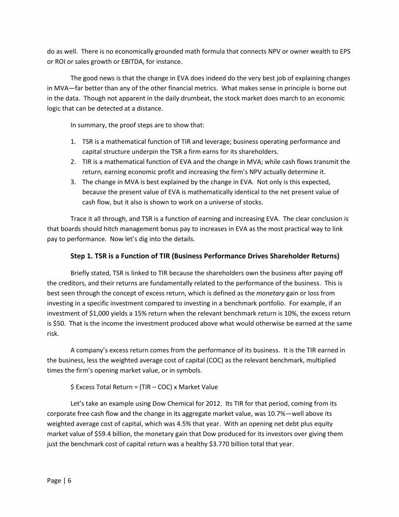
The chart below demonstrates this for Dow. It plots the firm’s total shareholder return each

year in red versus the total investor return earned in the business in blue. As predicted, Dow’s TSR

tracks but exaggerates the underlying swings in business performance. In 2008, for example, when

Dow’s business generated a negative 41.3% return, shareholders lost 57.5% of their wealth. The erosion

in shareholder value ended up dramatically increasing the firm’s leverage. The ratio of the firm’s overall

market value to its equity value ended 2008 at 1.9x, up from 1.3x the year the before. Good thing, too,

Page | 10

because in 2009, Dow’s business (and the stock market) recovered smartly and yielded a stunning 64.6%

return (albeit on a much depressed market valuation base), which when magnified by the leverage, gave

shareholders a nearly 87.1% return (to put that in perspective, though, the two year shareholder return

was still negative—almost -20%—which indicates why it is essential to view TSR over longer time

frames).

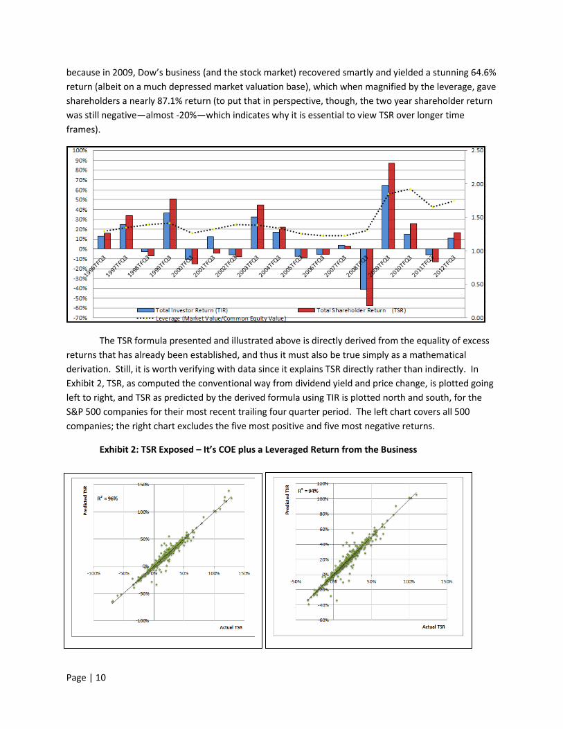
The TSR formula presented and illustrated above is directly derived from the equality of excess

returns that has already been established, and thus it must also be true simply as a mathematical

derivation. Still, it is worth verifying with data since it explains TSR directly rather than indirectly. In

Exhibit 2, TSR, as computed the conventional way from dividend yield and price change, is plotted going

left to right, and TSR as predicted by the derived formula using TIR is plotted north and south, for the

S&P 500 companies for their most recent trailing four quarter period. The left chart covers all 500

companies; the right chart excludes the five most positive and five most negative returns.

Exhibit 2: TSR Exposed – It’s COE plus a Leveraged Return from the Business

Page | 11

The regression is once again almost a perfect fit8. This proves yet again and perhaps more

explicitly that TSR is simply a math function of the TIR earned in the business, amplified by leverage. The

question now is, what determines TIR?

Step 2. TIR comes from earning EVA and increasing MVA

So far TIR has been described and computed as the free cash flow yield and the capital gain on

the firm’s market value. With a few substitutions, a firm’s TIR can be shown to come from its EVA profit

and the change in its aggregate MVA. To do this, we will use a few symbols and be a little more formal.

Once again, a firm’s TIR is defined to be the free cash flow (FCF) its business generates plus the

change in its overall market value (ΔV) divided by its market value at the start of the period (V0), or in

symbols, TIR = (FCF + ΔV)/V09. Now let’s play the substitution game.

Recall that a company’s free cash flow (FCF) is the difference between what it earns and what it

invests. It is the NOPAT (net operating profit after taxes) earned on the income statement less the

period change in the capital employed on its balance sheet, or in symbols, FCF = NOPAT − ΔCapital.

Also, since EVA = NOPAT − Capital Charge, we can rearrange the terms to see that NOPAT =

Capital Charge + EVA. Plug in:

TIR = ( FCF + ΔV)/V0

TIR = (NOPAT − ΔCapital + ΔV)/V0

TIR = (Capital Charge + EVA − ΔCapital + ΔV)/V0

The last substitution is to recognize that a firm’s MVA, its market value premium to its invested

capital, can be represented by V − Capital, which means that the change in MVA can be written as the

offsetting changes in the two components, or ΔMVA = ΔV – ΔCapital. Substituting in, TIR reduces to:

TIR = (Capital Charge + EVA + ΔMVA )/V0

The revised formula shows that the total return a firm generates for all its investors from its

business performance is a strict math function of three factors that all come from the EVA model.

The first is the capital charge as a yield on the firm’s beginning value. Since the capital charge is

the weighted average cost of capital times the capital invested in net business assets, this factor builds

in a base rate of return to give the investors the return they expect for bearing risk (just as the expected

cost of equity is built right into TSR). Again, that’s sensible. As time passes and business performance

unfolds, investors will expect to earn a risk-adjusted return from the time value of the money and from

8 It’s not quite as perfect a fit because the prior regression correlated absolute money gains and losses, which introduces a size bias due to the

fact that larger companies tend to have larger gains and losses than smaller companies. A size connection can sometimes radically inflate the real significance of the relationship being studied, but that is not really true here. Even the size-adjusted, the TSR to TIR correlation is very highly significant. 9 In practice it gets a little more complicated when we consider excess cash holdings that are excluded from the definition of FCF but that can

also be paid our or accumulated in a period, or if a company spins off a major line of business, and so on. But those are details that do not alter the insights.

Page | 12

reversing the discounting process. It comes from how they priced the stock in the first place—not as the

simple sum of EVA profit they forecast, but as the discounted present value sum of the EVA they

forecast. This being the case, corporate and shareholder returns always need to be judged relative to an

appropriate benchmark return—or cost of capital if you will—since market prices always factor in the

expected returns from the get go. This only reinforces the importance of measuring corporate profit net

of the capital charge, for only by earning the charge can management hope to meet market

expectations at a minimum.

The second factor in the total business return formula comes from earning EVA, from producing

a true economic profit above the cost of capital. It’s one for one—the more EVA the firm earns, the

higher its total investor return will be (and that will be magnified by leverage into an even higher total

shareholder return).

The third factor is the return that comes from expanding owner wealth, from increasing the

firm’s franchise value, from achieving and positioning the company for a greater abundance of positive

NPV investments. In short, it comes from increasing MVA.

In principle—and this will be tested in the third proof step—MVA increases when the expected

present value stream of EVA increases, either from an increase in current EVA or from revised

expectations about future EVA improvements. In other words, the true drivers of shareholder returns,

beyond just passively reversing the discounting process, are earning and increasing EVA and increasing

expectations for earning even more EVA.

At this stage we have derived two equivalent expressions for TIR, the one based on cash yield

and capital gain, and the other flowing from EVA, as follows (with Dow’s 2012 figures plugged in below,

and presented over the full history in Appendix 2):

Cash Flow Formula

TIR = ( FCF + ΔV )/V0

10.9% = ( $1967.5 + $4483.8 )/$59430.5

EVA Formula TIR = (Capital Charge + EVA + ΔMVA + FCF Adjustment )/V0

10.9% = ( $2665.7 + $597.2 + $2932.4 + $256.0 )/$59430.5

The EVA version makes it apparent in a way the cash flow formula does not that the real key to

driving shareholder returns is not to generate and pay out cash. It is to invest and grow EVA—as much

as possible.

On a technical note, the EVA formula for TIR includes a term, called FCF Adjustment, which is

needed to reconcile the reported financials that are used to compute EVA with the firm’s actual cash

flows. One example of why this is necessary would be when a company takes a direct charge to its

retained earnings to retroactively conform to a new accounting pronouncement. In that case,

computing capital spending as the simple period to period change in the company’s book capital

understates it. To correct for this, the non-cash charge to retained earnings is folded back into the

Page | 13

change in book capital to estimate the company’s capital expenditures for the period, and it is thereby

correctly deducted from the company’s Free Cash Flow. To ensure that EVA and cash flow equate, non-

cash charges to retained earnings like that must also be deducted from the EVA return, as is shown for

Dow. This is not a conceptual deficiency with EVA but just a grubby reality of the accounting data that is

used in this analysis (which comes from Compustat, a service of Standard & Poors’).

The derivation shows that the two formulas are conceptually and mathematically equal, and

that TSR is in fact determined by EVA and the change in MVA. But as added confirmation, we computed

TIR both ways for the S&P 500 companies for the 2012 fiscal years and plotted the results in Exhibit 3.

This time the R-squared is 100%! The two are indeed identical, which now leaves only one unanswered

question to fully explain TSR. What financial performance measure best accounts for the change in

MVA? Put differently, what is the real key to creating wealth?

Exhibit 3: TIR is Exactly the Same Both Ways

Step 3. EVA is the Real Key to Creating Wealth and Driving Shareholder Returns

As Fortune’s editors put it in a September 1993 cover story, EVA is “the real key to creating

wealth.” It’s the real key because EVA mathematically discounts to the net present value of cash flow,

or what is the same, to the MVA of an entire company. To see why, look at this as a banker would.

Suppose a banker lends you $1,000, and then says, “You have two choices. You can pay back the $1,000

right now or over time. For example, you could pay back $100 a year over ten years, and as long as you

also pay a market rate of interest on the outstanding balance, the present value is same as retiring the

full $1,000 today.”

Page | 14

What is the analogy? Free cash flow deducts capital investment as a company spends it, right

up front. It puts all the pain first, and all the payoffs later. EVA, in contrast, deducts capital investment

over time, through cost of goods sold flowing out of inventories and with the depreciation of the

investments in fixed assets. But in exchange, EVA also deducts in each period the market rate of

interest—the cost of capital —on the outstanding and as yet un-recouped capital balance appearing on

the balance sheet. The present value is always the same either way. Yet EVA is better than cash flow as

a measure of value (and as a management tool) because it better matches the timing of cost and

benefit. It spreads out the total principal and interest charge for capital over the time horizon that the

capital is expected to contribute to profits, just is as if the balance sheet assets have been rented, which

means that the period-to-period change in EVA is a far more reliable indication of whether firm’s net

present value, and hence its MVA, is expanding or contracting.

The formal statement is that a company’s MVA at a point in time is governed by a discounting of

its expected future EVA profit. Even if investors are actually projecting and valuing cash flow, it will still

be true that MVA is governed by EVA as well, for cash flow and EVA discount to the same net present

Exhibit 4: EVA and MVA for Autozone

Autozone, a specialty retailer of auto

aftermarket products, illustrates the link between EVA

and MVA that is expected. The top chart plots

Autozone’s year-end market value, essentially its

enterprise value, given its share price, versus the capital

invested in its net business assets; the bottom chart

plots the resulting MVA against the EVA profit the firm

earned each year. From 1997 to 2012, the firm’s MVA

increased from $3 billion to $15 billion and in lockstep

with a notable and sustained uptrend in EVA profit.

MVA, moreover, tended to closely mirror the

movements in EVA profit. EVA thus has been a very

good profit performance proxy for wealth creation and

the generation of TSR at Autozone.

MVA and EVA moreover certify that the

company’s performance and governance have been

exemplary. One reason: Autozone has been an EVA-

focused firm, and bonuses are tied to increasing it.

Another reason is that management increased the firm’s

franchise value through logistics excellence, optimizing

store locations, merchandising mix, advertising and

pricing policies, and the like. Increasing MVA does not

occur in a vacuum. It stems from enhancing business-

model productivity and scaling profitable growth—

things that ought to be at the top of any board’s agenda,

and which are promptly and accurately registered in the

growth in EVA profit.

EVA/MVA charts for 9,000 companies can be

viewed at www.evaDimensions.com/EVAvsMVA

Page | 15

value as a purely mathematical matter. Because of this, the change in MVA over a period of time should

be highly correlated with the change in EVA over that time (refer to Exhibit 4 above for an example using

Autozone).

The correlation will not be perfect, though, because the MVA at the end of a period, which

determines the change in MVA over the prior period, will be based on the forecast for EVA extending

beyond that period. In other words, MVA is influenced by changes in the firm’s business prospects

extending well into future periods, and past trends in EVA can never fully predict that.

The correlation between changes in EVA and changes in MVA should increase as the observation

period is extended. A longer track record smoothes cycles, increases investors’ confidence in

established trends, and generally removes noise from the data. EVA should thus be a better MVA

predictor over a five-year interval than it is year to year, for instance, and it is. The correlation also will

vary by line of business and depending on how much the change in profit performance over a prior

period can be confidently extrapolated into future periods. One would expect, for example, and indeed

one finds, that changes in EVA are a relatively weak predictor of the change in MVA for oil and gas

drillers, for real estate firms, and for start-up biotech firms—for companies that have considerable value

in the ground, on the ground or in a developmental pipeline but which only flow into profits with a

considerable lag. That is not just a problem for EVA, but for any financial measure. On the other side,

EVA also should be a relatively better predictor of MVA, and it is, for consumer staples and products

where brands, once established, can create an enduring value.

This is the theory. Now to the test. We began by computing the size-adjusted change in MVA

for the S&P 500 so that companies that vary in size could be fairly compared on the regression scale.

Specifically, we calculated a statistic called MVA Momentum, which is the change in MVA divided by the

sales in the base period. In effect, it is the rate at which a firm expanded its franchise value relative to

the original size of its franchise. To capture a sufficiently long horizon, MVA Momentum was computed

over a five-year interval. A company’s 2012 MVA Momentum was computed by taking its MVA as of the

end of 2012, given its stock price, shares outstanding, and capital base at that time, minus the MVA it

recorded five years before, at the end of 2007, given its stock price, shares outstanding, and capital base

at that time, and dividing by its sales for 2007. Again, it measures the rate of growth in owner wealth

and franchise value, scaled to the sales size of the company. This is the variable we want to explain. The

sample covered was once again the S&P 50010.

The first and most promising candidate to explain MVA Momentum is EVA Momentum, which is

calculated in the same way. It is the change in EVA over the five-year interval, divided by the sales in the

2007 base period. It measures the point-to-point rate of growth in economic profit, scaled to the sales

10

Starting with the S&P 500, we removed 18 firms that lacked a full five years of data (such as Mead Johnson and Kraft Food Group that were

spun out of larger companies), and 22 firms that had undertaken large spinoffs (such as Tyco), leaving 460 firms. Then, we removed a set of long lead time firms, which covered all 14 real estate firms, the one biotech firm in the S&P500 with revenues under $5 billion, and 11 small and mid-tier oil and gas firms with revenues under $10 billion, leaving a total of 435 firms in the study. The data set was further pruned through Winsorization to eliminate outliers (firms with variable observations that were outside a plus and minus three standard deviation band around the average) in order to focus on the more normal observations. Lastly, in each regression we removed “misfits,” the twenty firms that had the largest divergence between the percentile rank of MVA Momentum and the rank of the variable being regressed. Refer to Appendix 4 for more details.

Page | 16

size of the company. EVA Momentum measures the growth rate in quality earnings, not total earnings,

and thus it should best explain the growth in MVA, or MVA Momentum. The other candidates examined

are:

Net Income Momentum (measured the same way, as the change in reported net

income before unusual items, divided by base period sales)

EPS Momentum (the change in basic EPS, excluding unusual items, times the number of

shares outstanding at the end of the base period, divided by base period sales. It

measures the growth rate in the net income attributable to an investor who held all the

shares outstanding as of five years ago while suffering dilution from new share

offerings and without participating in share buy-backs over the subsequent five year

interval; unlike growth in EPS, EPS Momentum is meaningful even when base period

EPS is negative or negligible)

EBITDA Momentum (the same, measured as the change in the firm’s EBITDA/base

period sales)

Change in EBITDA Margin (EBITDA/Sales in 2012 less the ratio in 2007)

Sales Growth Rate (same, the change in sales/base period sales)

Free Cash Flow Generation (same, cumulative five-year FCF/base period sales)

Return on Capital (NOPAT/Average Capital, in the latest period), and lastly

Change in Return on Capital over the five-year interval

All the candidate measures (except the return measures and the change in EBITDA margin) are

scaled by base period (2007) sales in order to align with MVA Momentum, which is also scaled by sales

in the base period. The variables were regressed one by one against MVA Momentum in three ways.

The first used the raw values. In the second, the variables were first ranked and the regression was

performed on the percentile values. The third also used the percentile rank values but with the added

requirement that the regression pass through the origin, that is, that the zero percentile scores for both

variables must be the starting point on the regression line.

The percentile regressions test the ability of each variable to rank order MVA Momentum as

opposed to literally predicting each observation. Requiring the percentile regression to pass through

the origin sensibly asks how well the percentiles scores line up when they are forced to intersect at the

starting percentile ranks and not arbitrarily along the way. That is the strictest test of alignment and will

be accorded the most significance11. After all, ISS will use TSR to rank pay versus performance versus

peers, so the real question is which corporate performance variable is best rank correlated with MVA

Momentum and thus TSR. The slope of that regression line will also be telling. The closer to one it is,

the more MVA Momentum and the explanatory variable are aligning all through the percentile ranks.

11

Forcing the regression to pass through the origin can result in negative R-squared. That is because R-squared is measured relative to the

assumption no correlation exists between the two variables, and the squared errors against a flat line are summed as the reference deviation. If a regression line forced to pass through the origin leads to a greater sum of squared errors compared to the actual observations than the reference sum, then the R-squared of that regression line is negative. It is worse than assuming there is no correlation at all, which is the case with EBITDA Momentum, FCF Generation, Return on Capital, and Sales Growth.

Page | 17

The findings are summarized in the table and chart below (the regression plots for all the variables are

presented in Appendix 3, and details of the statistical analysis are presented in Appendix 4).

Exhibit 5: EVA is Really the Key to Creating Wealth

The findings are as follows:

Generating “free cash flow” net of investment spending does not matter. It is

consistency uncorrelated with creating wealth and driving TSR, because the market does

not want cash, it wants investments that will grow value. A good example has been

Amazon, which poured capital into EVA-positive growth over the past five years, leading

to a starkly negative FCF but a very strong stock market and MVA performance.

Ironically, the cash flow measure that is projected and discounted to measure value, and

which appears in the definition of TIR, is almost completely uncorrelated with whether

companies are actually creating value and generating an outstanding shareholder

return. The conclusion is clear: Boards should never pay management to generate cash

flow12.

12

A private company or private equity company may feel it is wise to pay managers to generate free cash when cash is limited. But that is

blunt instrument that ends up slaying the innocent with the guilty. It discourages all investment in a period regardless of merit. A better solution is to reward management for increasing EVA, but where EVA is measured using an artificially inflated cost of capital—up to several percentage points over its true public market rate. Raising the rate sweats more cash out of balance sheet assets and cuts off at the knees projects that would otherwise be accepted. It directly attacks the problem that capital is extra scarce by making it extra costly rather than

Page | 18

Earning a high return on capital is no guarantee of stock market success. The only rate-

of-return variable that matters at all is increasing ROI. The level of ROI is largely known

and in the stock price. It’s the improvement in return that matters, but it is not all that

matters. Growth matters, too, of course, and it becomes an even more important

consideration over longer time horizons like the five-year interval examined here. In

any form, level or change, ROI is demonstrably a far less effective valuation metric than

EVA. Boards should abandon ROI. It is a suffocating measure that stifles innovation and

deters initiative and stops profitable growth in its tracks.

Growth matters, but sales growth is apparently a very poor measure of the growth that

counts – it can be manufactured by bulking up on operating costs and investments.

Despite its popularity among the private equity crowd, EBITDA is a very poor measure of

wealth creation and at its best not half as good as EVA. EBITDA is blind to earning a

decent return on invested capital, to the necessity of replacing wasting assets, to paying

taxes, to covering investments in acquisition goodwill, to a firm’s pension funding status,

and a lot more. It is truly earnings before many things that count.

Net Income growth is hands down better than EBITDA. At least it factors in

depreciation, taxes and borrowed money interest expense as legitimate business costs

that EBITDA blithely ignores. But it too has blind spots. It does not set aside a return for

the shareholders, and it is riddled with accounting distortions that EVA repairs.

Though closely related, EPS Momentum provides a notable improvement on Net

Income Momentum because it does account for the cost of equity capital in a way,

through the dilutive or accretive effects of issuing or retiring shares over the interval.

However, it accounts for the cost of capital rather clumsily, episodically, and

incompletely—it ignores the cost of using retained earnings to finance growth. Also,

from a practical standpoint, it cannot be computed at a business unit or division level

and cannot be used in modeling the economics of individual business decisions. And

like net income, it is subject to the foibles of reported accounting.

Taking a big step forward, the clear winner is EVA Momentum. Driving growth in real

economic profit after setting aside a priority return for the owners and cleansing

accounting distortions is indeed the real key to creating wealth and the true driver of

TSR. Moreover, unlike EPS, it can be computed and managed within the lines of

business. It can be projected, analyzed and discounted to help line teams to measure

and improve the NPV of their plans, projects, acquisitions and decisions. It is not just an

elitist corporate measure. It’s a boots-on-the-ground measure that operating teams can

use to run their businesses in ways that directly contribute to increasing the corporate

TSR.

EVA Momentum not only has the highest R-squared across all regressions. It is by far the best at

the percentile regression, which means it’s the very best measure to rank order TSR. Moreover, the

slope of the EVA Momentum percentile regression with MVA Momentum is exactly 1.0 where all the

attacking the cash flow symptom. Put simply, never ration capital, charge for it at a market clearing rate, even if the market for capital is established inside the company.

Page | 19

other measures have slopes less than 1.0. EVA Momentum is not only the best at explaining the rank

order of wealth creation. It is the most correctly aligned with it as well.

The following examples deal with instances where performance measured by EVA Momentum

differed significantly from other measures. In discussing them, I explain why the answers provided by

EVA are more economically sensible and, as a result, track MVA and TSR more closely.

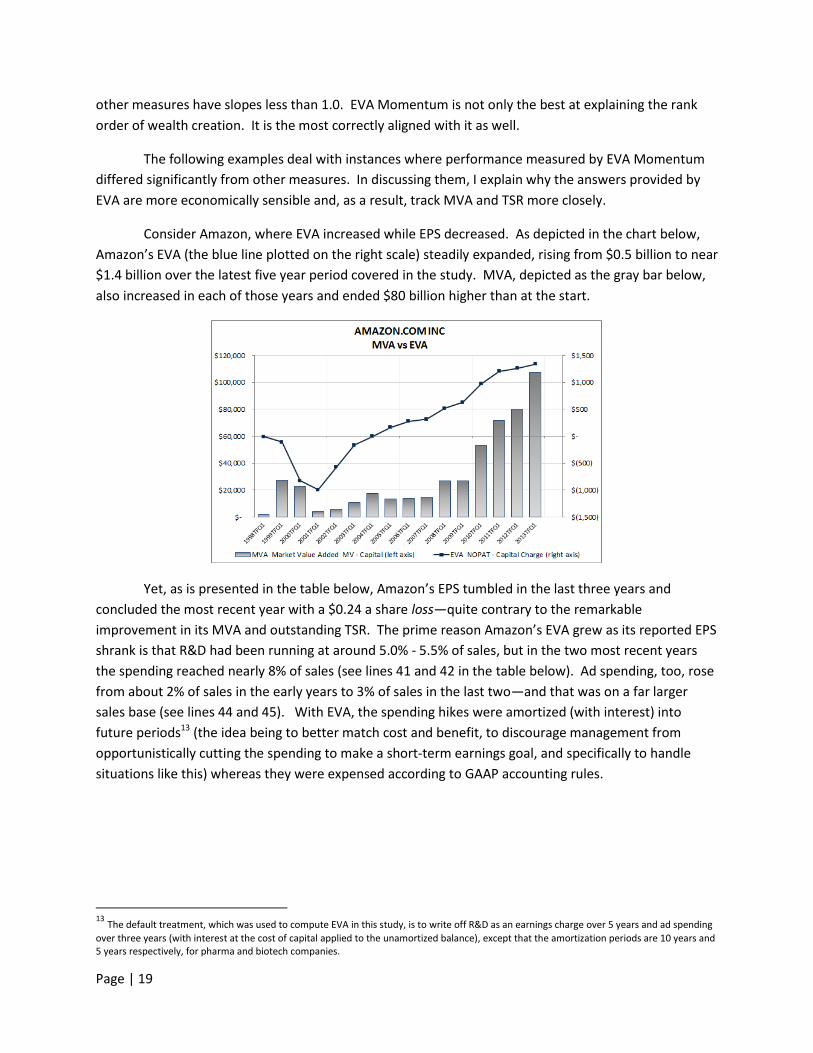
Consider Amazon, where EVA increased while EPS decreased. As depicted in the chart below,

Amazon’s EVA (the blue line plotted on the right scale) steadily expanded, rising from $0.5 billion to near

$1.4 billion over the latest five year period covered in the study. MVA, depicted as the gray bar below,

also increased in each of those years and ended $80 billion higher than at the start.

Yet, as is presented in the table below, Amazon’s EPS tumbled in the last three years and

concluded the most recent year with a $0.24 a share loss—quite contrary to the remarkable

improvement in its MVA and outstanding TSR. The prime reason Amazon’s EVA grew as its reported EPS

shrank is that R&D had been running at around 5.0% - 5.5% of sales, but in the two most recent years

the spending reached nearly 8% of sales (see lines 41 and 42 in the table below). Ad spending, too, rose

from about 2% of sales in the early years to 3% of sales in the last two—and that was on a far larger

sales base (see lines 44 and 45). With EVA, the spending hikes were amortized (with interest) into

future periods13 (the idea being to better match cost and benefit, to discourage management from

opportunistically cutting the spending to make a short-term earnings goal, and specifically to handle

situations like this) whereas they were expensed according to GAAP accounting rules.

13

The default treatment, which was used to compute EVA in this study, is to write off R&D as an earnings charge over 5 years and ad spending

over three years (with interest at the cost of capital applied to the unamortized balance), except that the amortization periods are 10 years and 5 years respectively, for pharma and biotech companies.

Page | 20

The amortized charge to EVA, even including the interest on the prior unamortized spending,

was about 6.3% of sales in the most recent period (the sum of lines 40 and 43 above) as compared to a

book profit charge of 10.8% of sales ( the sum of lines 41 and 44 above). The 4.5% difference is why EPS

recorded a loss and EVA a win. EVA simply does a better job than EPS of distinguishing investments

from expenses, and more correctly measures the true period cost and real profit performance of

companies like Amazon that are accelerating investments in intangible assets and proprietary

capabilities and brand strength to enhance their long-run value. Netflix provides a similar example and

is reviewed in Appendix 5.

Another distortion occurs when EVA goes down as EPS goes up, which is fairly common. A total

of 198 companies in the sample universe produced significant EPS Momentum, defined as Momentum

above 2.5% over the five years (or better than a 0.5% average per annum). Of those, 33 firms, or one

out of six, produced a negligible EVA Momentum or worse. Nineteen had very modest EVA growth,

which was defined as less than 2% overall, as shown in the table below, and fully 14 of the 33 had

negative EVA Momentum. Of those 33 firms where EPS Momentum was strongly positive and

significantly overstated EVA Momentum, 23 suffered declines in MVA. They destroyed owner wealth

over the five years even as their EPS increased materially. Of the remaining 10 firms, 2 generated less

Page | 21

MVA Momentum than the sample average, and 5 just matched the sample average. Only 3 of 33

managed to produce above average Momentum, and the highest was only 0.4 standard deviations

above the average, indicated by the Z-Score14. Clearly, the market was far more responsive to EVA than

EPS when setting the values for these stocks.

The largest discrepancy between EVA Momentum and EPS Momentum was exhibited by First

Solar. Its EPS grew from $1.87 to $5.74 from 2007 to 2012, equivalent to EPS Momentum of 48.3% over

the five years, or the 98th percentile of all firms. At the same time, its EVA plummeted from $81 million

to a $7 million loss, for a cumulative EVA Momentum of -13.7%, so low that it was in the third percentile

from the bottom of the S&P sample (see Appendix 6 for a fuller explanation of the EPS to EVA gap).

How did MVA respond? As was typical of the entire group, First Solar’s MVA followed its EVA down, not

its EPS up. In fact, its MVA fell so dramatically—from positive $17 billion to negative $2 billion—that it

was ranked as the very worst MVA wealth destroyer in the S&P15.

14

Z-Score is the number of standard deviations a variable is away from the average. It is computed by taking the observed value, less the

sample average value for the variable, and dividing by the standard deviation exhibited by the variable. 15

Although First Solar clearly demonstrates the superiority of EVA compared to EPS as a predictive metric, it was not included in the regression

statistics. Its MVA Momentum was so negative it was deemed to be an outlier and was removed from the study so as not to bias the statistics with an extreme observation. Including it would have tipped the scales way in favor of EVA as compared to EPS.

Page | 22

How can a company’s EVA shrink or only grow very slowly as its EPS expands significantly? Said

another way, what accounts for the divergent results registered by the firms in the table above? The

reasons vary, but our analysis shows it includes the following:

1. Investments in business assets that exceeded the cost of borrowed money but that failed to

cover the full cost of capital, including the cost of retained earnings, was a fairly common

occurrence

2. Debt-financed share buybacks or acquisitions that boosted EPS but not EVA

3. Restructuring charges that were washed out of EPS but which were capitalized and turned

into capital charges against EVA

4. R&D and advertising spending that failed to generate a return sufficient to cover the

amortized cost, with interest, that was spread into subsequent periods under EVA but not

with EPS (essentially the opposite of what happened at Amazon)

5. Recognition of a deferred tax asset, which was assessed a capital charge in EVA but none in

EPS

6. A reduction in pension funding status which is converted into a cost of capital charge to EVA

but is either ignored or smoothed into profits over a very long time frame under EPS

Investors are generally well aware of these distortions and take them into account when setting

share prices, which is why EVA far more accurately tracks market prices than the reported earnings

figures do. Investment analysts, after all, actually analyze stocks and closely scrutinize the footnotes, a

firm’s efficiency in using capital, its leverage ratio, and the myriad factors that fundamentally influence

the quality of its earning and its intrinsic value, which is why when a company’s reported EPS increases,

and its EVA and MVA decrease, investors simply end up assigning a lower price/earnings multiple to the

stock in recognition that the true quality of its earnings is less than it is reported to be.

Let’s now contrast EVA Momentum with the change in Return on Capital (ROC), which was also

a relatively highly rated metric, by looking at a group of companies that generated nearly the same

improvement in return on capital but with very different EVA and MVA results. The eight companies

selected are presented in the table below. They were chosen because they followed each other in rank

when all firms in the sample universe were ordered by the change in return on capital, and because they

all managed to produce a substantial improvement in their returns, ranging from a 5.7% uptick to a 6.2%

ROI breakout over the past five years (equivalent to about one-half a standard deviation above the

average change, as indicated by the Z-Scores). In sum, all these firms managed to improve their return

on capital in a statistically meaningful and to an essentially equivalent degree.

Despite the ROI similarities, the MVA Momentum the firms produced over the five year interval

varied significantly, from a soaring 502% for Chipotle Mexican Grill to a loss of 11% for Valero. The

variable that far better explains the divergent valuation outcomes is EVA Momentum. The EVA

Momentum Z-scores—the number of standard deviations above or below the mean Momentum—were

+0.8 to +0.9 for the two biggest stock gainers (Chipotle and Monster Beverage), were negative for the

three weakest performers (Valero, Marriott, and AmerisourceBergen), and were +0.2 to +0.3 for the

three middle of the road stock performers. In short, the correlation of wealth creation was much

Page | 23

stronger with EVA Momentum than with the change in the return on capital, because EVA Momentum

considers risk, growth, and the concluding level of the return on capital, and not just the change.

EVA Momentum performed so much better than ROI on these stocks because it not only

measured the improvement in profitability. It also implicitly incorporated the value added by the

growth the companies achieved. Indeed, it is the only corporate performance score that takes all

performance dimensions into account. It does not have the blind spots that other measures have. To

see this, let’s deconstruct EVA Momentum into two main drivers from which all others can be derived.

The first way to increase EVA and generate Momentum is to improve EVA Margin, that is, to increase

the ratio of EVA to sales by dropping more EVA to the bottom line out of top line revenues. That

indicates the firm has improved the productivity and profitability of its business model spanning income

statement efficiency and balance sheet asset management. It has done this through some combination

of what we like to call the three-“P’s”—price, product and process, that is, from earning and exerting

price power, from fielding an outstanding EVA-positive product line-up and benching losers, and from

process excellence, from running a tight ship with operational excellence and lean capital management.

Those are the types of initiatives that return on capital also tends to measure and emphasize. But EVA

Momentum goes beyond just measuring gains in productivity and business model profitability and

includes a second component which covers the value of profitable growth—a performance dimension

that ROI or profit margin in any form completely ignore.

The second way to increase EVA and drive Momentum is to generate positive sales growth at a

positive EVA Margin. This factor is literally the product of the firm’s sales growth rate times its

concluding EVA profit margin. For example, suppose a company realized productivity gains and

improved its EVA Margin from 4% to 5%, and suppose further that it generated 20% sales growth over

the period. Then its EVA Momentum would come in at 2%, with 1% coming from getting better, from

improving the EVA Margin, and the other 1% coming from getting bigger, from delivering 20% sales

growth at a 5% EVA Margin.

Take Monster Beverage, one of the companies in the table, as an example. Its EVA Momentum

over the five years was 17.5%. That’s the overall increase in its EVA as a percent of base period sales,

and it had to come from a combination of getting better and getting bigger. Surprisingly, its EVA Margin

shrank a bit. It dropped from 16.6% to 15.5%, for a 1.1% decrease that served to reduce its EVA

Momentum. As is typical of companies as they scale a highly profitable business formula, Monster had

Page | 24

to give up a portion of its pricing power and business productivity as it grew. But Monster way more

than compensated for that shortfall with exceptional profitable growth. Its sales surged from $950

million to $2.1 billion, for 120% sales growth overall and a CAGR of 17.1% over the interval. The sales

that Monster added effectively added to its EVA at its concluding 15.5% EVA Margin rate, for a total

profitable growth contribution of 18.6% (120% x 15.5%). Put it together, and the Margin loss of 1.1%

plus the profitable growth gain of 18.6% fully accounts for the firm’s terrific 5-year EVA Momentum of

17.5%. Incidentally, over the same interval, Monster’s return on capital increased by 5.7%, impressive

on its own, but nevertheless a result that completely understates the firm’s actual accomplishment and

that entirely overlooks the true source of its phenomenal shareholder return.

In sum, unlike any other measure, EVA Momentum combines productivity gains and profitable

growth into one overall score of economic profit progress. It is uniquely capable of measuring the total

value added in a period from all sources. To recreate all the performance dimensions that EVA

Momentum packs into one grade you would have to blend together the change in return on capital, the

ending return on capital, the cost of the capital, and the firm’s growth rate in some unfathomably

complex and non-linear combination. Of course, that can never be done accurately and without

significant complexity. At the best you would end up with a highly imperfect and impractical proxy for

just using EVA and EVA Momentum to score performance and run a business.

As a final note, and as expected, the correlation between EVA Momentum and MVA Momentum

varies by sector. The table below presents the R-squared from percentile regressions forced through

the origin for 24 industry groups covering an expanded universe of the Russell 3000 companies.

Page | 25

The weighted average R-squared across all the companies covering all the industry regressions

was 65%, which is about 7% better than the 58% R-squared recorded for the S&P 500 run. The modest

improvement is due to using more companies, to fitting each industry with its own regression run, and

to more extensively pruning the data set (approximately 23% of the eligible firms were eliminated as

either outliers or misfits in the industry regressions runs versus only about 8% (35 out of 434 firms) in

the S&P 500 run).

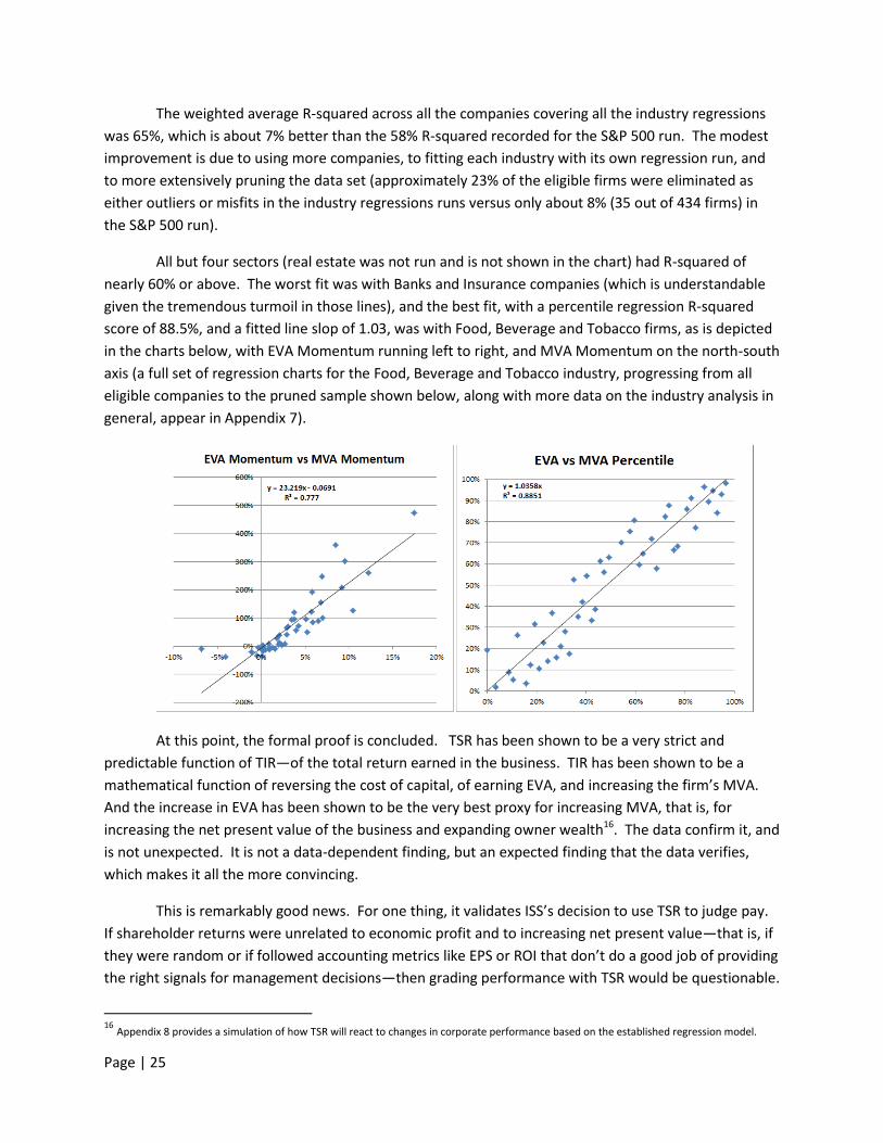
All but four sectors (real estate was not run and is not shown in the chart) had R-squared of

nearly 60% or above. The worst fit was with Banks and Insurance companies (which is understandable

given the tremendous turmoil in those lines), and the best fit, with a percentile regression R-squared

score of 88.5%, and a fitted line slop of 1.03, was with Food, Beverage and Tobacco firms, as is depicted

in the charts below, with EVA Momentum running left to right, and MVA Momentum on the north-south

axis (a full set of regression charts for the Food, Beverage and Tobacco industry, progressing from all

eligible companies to the pruned sample shown below, along with more data on the industry analysis in

general, appear in Appendix 7).

At this point, the formal proof is concluded. TSR has been shown to be a very strict and

predictable function of TIR—of the total return earned in the business. TIR has been shown to be a

mathematical function of reversing the cost of capital, of earning EVA, and increasing the firm’s MVA.

And the increase in EVA has been shown to be the very best proxy for increasing MVA, that is, for

increasing the net present value of the business and expanding owner wealth16. The data confirm it, and

is not unexpected. It is not a data-dependent finding, but an expected finding that the data verifies,

which makes it all the more convincing.

This is remarkably good news. For one thing, it validates ISS’s decision to use TSR to judge pay.

If shareholder returns were unrelated to economic profit and to increasing net present value—that is, if

they were random or if followed accounting metrics like EPS or ROI that don’t do a good job of providing

the right signals for management decisions—then grading performance with TSR would be questionable.

16

Appendix 8 provides a simulation of how TSR will react to changes in corporate performance based on the established regression model.

Page | 26

But our research shows it makes sense. Granted, that is not obvious when TSR is expressed as a

dividend yield and capital gain. It is also not obvious or even true in the hurly burly of day-to-day or

even year-to-year trading activity, just as it is not apparent that a casino always wins. But when one

steps back and traces TSR to its roots, which are indeed economically grounded and firmly tied to EVA

and increasing NPV, and when one studies aggregate stock price behavior over a strategic horizon like

five years (as one might aggregate all the bets at a casino over a meaningful period), the logic of using

TSR to judge pay shines through.

The finding is also fantastic news for boards and management teams. It gives them a practical

way to manage for higher TSR. On the one hand, boards can reward managers for increasing EVA and

be highly confident that their pay plans will pass the ISS test17. But as important, EVA can help

managers to improve their firm’s TSR performance. EVA—or rather, EVA Momentum—is the bottom-

line score in a financial management framework that can provide every manager, and even rank-and-file

employees, with practical, easy-to-understand information they need to make the most value-enhancing

decisions.

The bottom line is this. If TSR is the question, EVA is the answer.

(The full report, What Determines TSR, can be downloaded at www.evaDimensions.com/EVA2TSR/report)

17

EVA can be used in bonus plans that accurately emulate the incentives of an owner. One example is a plan that pays a base bonus, which

brings total pay to market, plus a percent of the change in EVA over the prior year. This provides managers with the incentive to use EVA as a management tool and to make decisions that will increase it. The plan also pays managers for creating value by sharing the value they create with them, and not for beating a budget. It liberates managers to think and act like charged up owners and to collaborate as a team to deliver outsized EVA improvements over a strategic horizon. It also aligns pay to performance in accord with ISS’s goals. For instance, if EVA moves sideways and does not change, so that investors just earn the cost of capital they expect to earn on any newly invested capital, then the management teams just earns the base bonus they expect. But the more management is able to improve EVA, and thus improve the firm’s NPV and TSR, the bigger its bonus—which means that over time, management’s true bonus (the bonus over the base bonus) is perfectly aligned with the excess returns generated for the owners. In practice, the simple bonus plan outlined here can be modified to accommodate specific circumstances. For instance, the change in EVA could be measured relative to the projected increase in EVA that is baked into the stock prices of growth companies, and the change could be measured relative to peers for cyclical stocks. One way to do that is to hitch the bonus to the firm’s realized EVA Momentum compared to the EVA Momentum achieved by the median competitor firm.

Bennett Stewart is an expert in shareholder value and corporate

performance management, author of Best-Practice EVA (John Wiley &

Sons, March, 2013), and CEO of EVA Dimensions, a financial

technology firm that provides software tools, data bases and training

and support packages that help CFOs to test and automate Best-

Practice EVA and investors to make better buy-sell decisions.

He can be reached at gbstewart@evadimensions.com

Page | 27

Appendix 1: The Full Excess Returns History Shows They Closely Match for Dow

Page | 28

Appendix 2: TIR Computed Two Ways – with FCF and with EVA – are the Same for Dow

Page | 29

Appendix 3: S&P 500 Regression Plots

The left hand plots are from the regression of the raw variables against MVA Momentum, and

the right charts are percentile rank regressions, with the upper right result forced through the origin.

Page | 30

Page | 31

Page | 32

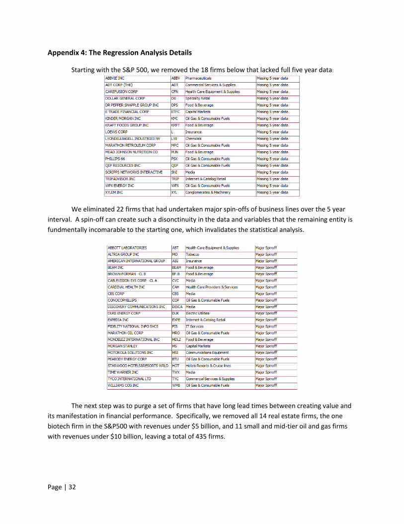
Appendix 4: The Regression Analysis Details

Starting with the S&P 500, we removed the 18 firms below that lacked full five year data:

We eliminated 22 firms that had undertaken major spin-offs of business lines over the 5 year

interval. A spin-off can create such a disonctinuity in the data and variables that the remaining entity is

fundmentally incomarable to the starting one, which invalidates the statistical analysis.

The next step was to purge a set of firms that have long lead times between creating value and

its manifestation in financial performance. Specifically, we removed all 14 real estate firms, the one

biotech firm in the S&P500 with revenues under $5 billion, and 11 small and mid-tier oil and gas firms

with revenues under $10 billion, leaving a total of 435 firms.

Page | 33

Next, following the standard procedure, called “Winsorization,” we pruned the data set to

eliminate companies with extreme MVA Momentum observations. We did this so as not to bias the

regression statistics with the influence of outliers and in order to isolate the ability of the financial

variables to explain the more normal MVA Momentum observations. The outliers are defined as firms

with observations falling outside a plus and minus 3 standard deviation band around the average. This

eliminated six companies (or 1.6% of the 435 remaining firms) with extreme positive MVA Momentum

and First Solar, the one with the very lowest MVA Momentum.

A company’s Z-Score is its company’s 5 year MVA Momentum minus the sample average divided by the standard deviation. It’s the number of

standard deviations away from the average. All companies with MVA Momentum Z-scores outside the range of + or – 3 were removed.

We also eliminated the outliers for each individual variable, i.e., we removed those companies

having the most extreme observations falling outside the three standard deviation band exhibited by

each variable. For example, the ten companies listed below were the EVA Momentum outliers, of which

two were also MVA outliers, for a net eight additional exclusions from the EVA Momentum regression

with MVA Momentum:

Page | 34

Unfortunately, Apple and Priceline, which were exemplary creators of EVA and MVA, were

excluded from the study, but leaving them in would bias the regression statistics for companies that

were not at the extreme tail end of the distribution.

The eight companies listed below were EPS Momentum outliers, of which three were also MVA

outliers, for a net of five firms (1.1% of the sample) excluded from the EPS Momentum regression with

MVA Momentum:

Seven outliers were common to EPS and EVA, and only four in total were unique.

Lastly, in each regression we removed twenty “misfits,” or approximately 5% of the remaining

sample that were found to have the largest disagreement between their MVA Momentum rank and the

rank for the variable being regressed. For example, the tables below present the twenty companies that

had the largest discrepancy between the direction of their MVA and the direction of their EVA and their

EPS over the five years, and which were thus removed from the EVA and from the EPS regressions,

respectively. Removing the misfits enabled the more characteristic and typical relation with MVA

Momentum (and thus TSR) to shine through in the case of each regression.

Page | 35

EVA Misfits

EPS Misfits

Nine of the twenty misfits were common to EVA and EPS. The average tracking error was 69

percentile points for the EVA “misfits” and 75 percentile points for EPS. The EPS misfits included

Amazon and NetFlix which were firms where EVA Momentum closely tracked MVA Momentum.

Page | 36

Let’s examine a few of the firms that were excluded from the EVA regression. Monsanto was

rated to have one of the largest disconnects between its EVA Momentum and MVA Momentum over the

past years, and was removed as a “misfit,” yet that appears truly to be just a statistical aberration.

Monsanto’s MVA is plotted in the chart below as a gray bar, reflecting the share price at the end of each

reporting period, and its EVA profit earned over the prior four quarter period is plotted as the blue line,

on the right scale. Over the years a generally rising EVA tide has lifted the MVA ship, and movements in

Monsanto’s EVA have generally been reflected in its MVA, as expected. Yet, taking the five year point to

point change from 2007 to 2012, MVA was down and EVA was up. The disconnection is just a matter of

timing.

Newmont Mining also had one of the largest gaps between its EVA and its MVA over the past 5

years. Its EVA profit increased mightily while its MVA plunged. Newmont mines and sells gold. Its share

price at the end of each period and thus its MVA is affected by reserves in the ground and the spot and

future price of gold, which investors use to forecast its EVA profits. In contrast, its EVA reflects the

profits actually earned from production over the prior period and the average price of gold in the

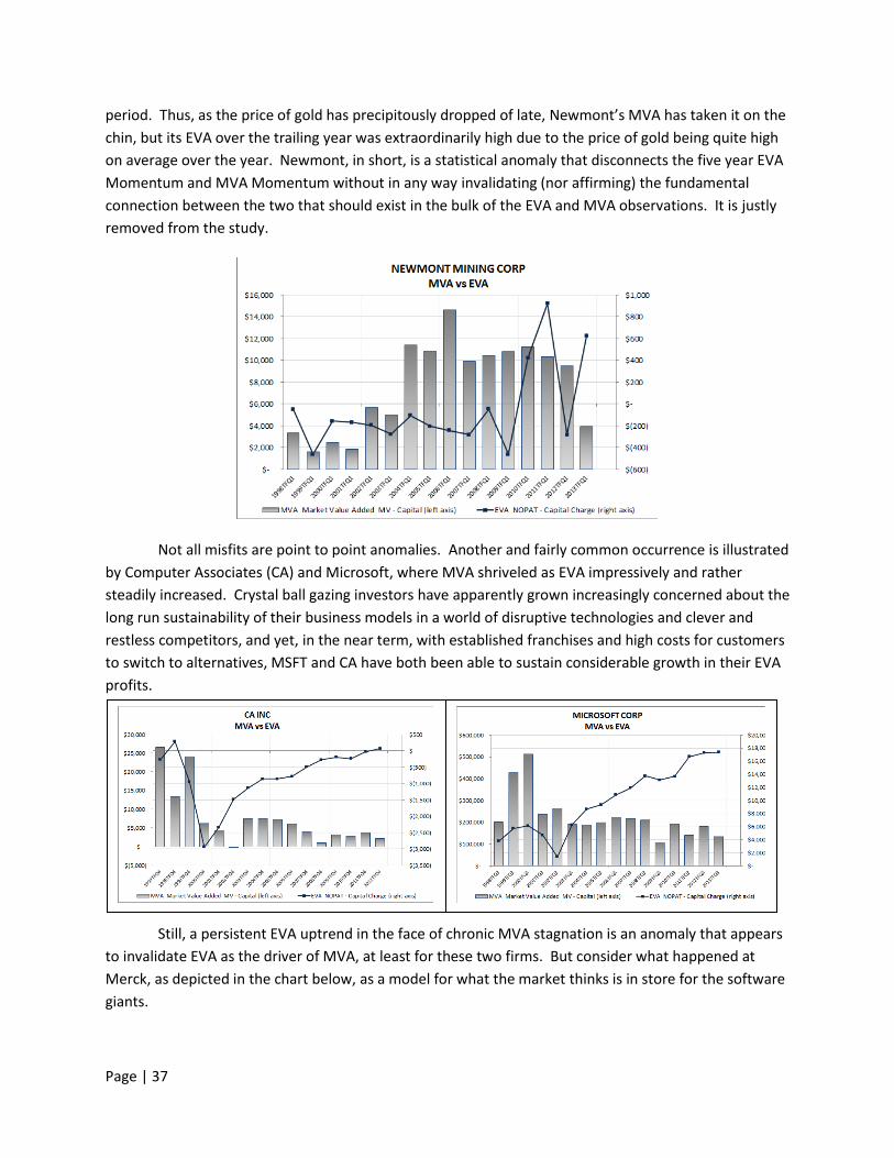
Page | 37

period. Thus, as the price of gold has precipitously dropped of late, Newmont’s MVA has taken it on the

chin, but its EVA over the trailing year was extraordinarily high due to the price of gold being quite high

on average over the year. Newmont, in short, is a statistical anomaly that disconnects the five year EVA

Momentum and MVA Momentum without in any way invalidating (nor affirming) the fundamental

connection between the two that should exist in the bulk of the EVA and MVA observations. It is justly

removed from the study.

Not all misfits are point to point anomalies. Another and fairly common occurrence is illustrated

by Computer Associates (CA) and Microsoft, where MVA shriveled as EVA impressively and rather

steadily increased. Crystal ball gazing investors have apparently grown increasingly concerned about the

long run sustainability of their business models in a world of disruptive technologies and clever and

restless competitors, and yet, in the near term, with established franchises and high costs for customers

to switch to alternatives, MSFT and CA have both been able to sustain considerable growth in their EVA

profits.

Still, a persistent EVA uptrend in the face of chronic MVA stagnation is an anomaly that appears

to invalidate EVA as the driver of MVA, at least for these two firms. But consider what happened at

Merck, as depicted in the chart below, as a model for what the market thinks is in store for the software

giants.

Page | 38

Starting as far back as 2002, Merck’s MVA began to plummet (ultimately falling from $150 billion to

about $45 billion at present), and yet, in similar vein to MSFT and CA, its EVA continued on a positive

trend growth path over the next seven years based on scaling its established product portfolio.

Investors were apparently looking far down the road and becoming increasingly worried that Merck

would be unable to replace patent expirations with blockbuster drug discoveries, and they presciently

marked the share price down well in advance of the eventual and it seems now inevitable downturn in

EVA, which started in 2008-2009. Merck’s EVA has since fallen from a peak of $5.5 billion to $3.3 billion.

If one time-shifted Merck’s EVA 5 to 7 years leftward on the chart, back towards prior MVA

observations, then a close association between movements in EVA and movements and MVA would be

observed. EVA, no doubt, is still the key to creating—or destroying wealth—but the linkage does not

always play out over five years (even so, Merck is in the study, it is neither an outlier nor a misfit, and

the disassociation between its EVA and MVA is one of the observations that served to reduce the R-

squared of the EVA Momentum regression).

The insight is that firms like these that have strong franchises established through patent

protection or a widely-installed customer base can continue to generate EVA growth for some long time,

for five to seven years or longer, before the tectonic plates shift and the downturn the market has

forecast comes to pass. The implication is that CA and Microsoft are simply farther behind on the path

that Merck has already trodden, and that someday their EVA, too, will fall in line with their depressed

MVA valuations. Similar conclusions apply also to other tech firms on the misfit list, like Western Digital

and Intel, as well as medical technology companies Like Medtronic and Stryker shown in the charts

below that have managed to sustain growth in EVA while the sword of Obamacare dangles over their

heads.

Page | 39

Remember, these are the egregious exceptions and not the rule. The rule is that the change in

EVA does the best job of any financial metric in explaining the change in MVA.

Page | 40

Appendix 5: Like Amazon, Netflix is an EPS Loser but an EVA and MVA Winner

Page | 41

Appendix 6: First Solar’s EPS Rises While its EVA and MVA fall

There are several reasons why First Solar’s EPS and EVA diverge so sharply. First Solar runs a

capital intense business that has become more intense. Its working capital investment, for example,

increased from about 40 to 130 days (line 36), which took the pre-tax cost of capital charge from 2.3% of

sales to 6.3% of sales (line 35). Yet, that charge is ignored in EPS. First Solar also took sizable

restructuring and impairment charges two years back, which have been carried forward as capital,

subject to a capital charge, in the most recent year—but that was ignored under EPS. The charge is a

component in the Corporate Charges line item (line 47), which increased in proportion to pre-tax EVA.

All told, First Solar is a textbook example of how EPS can misrepresent true performance and value.

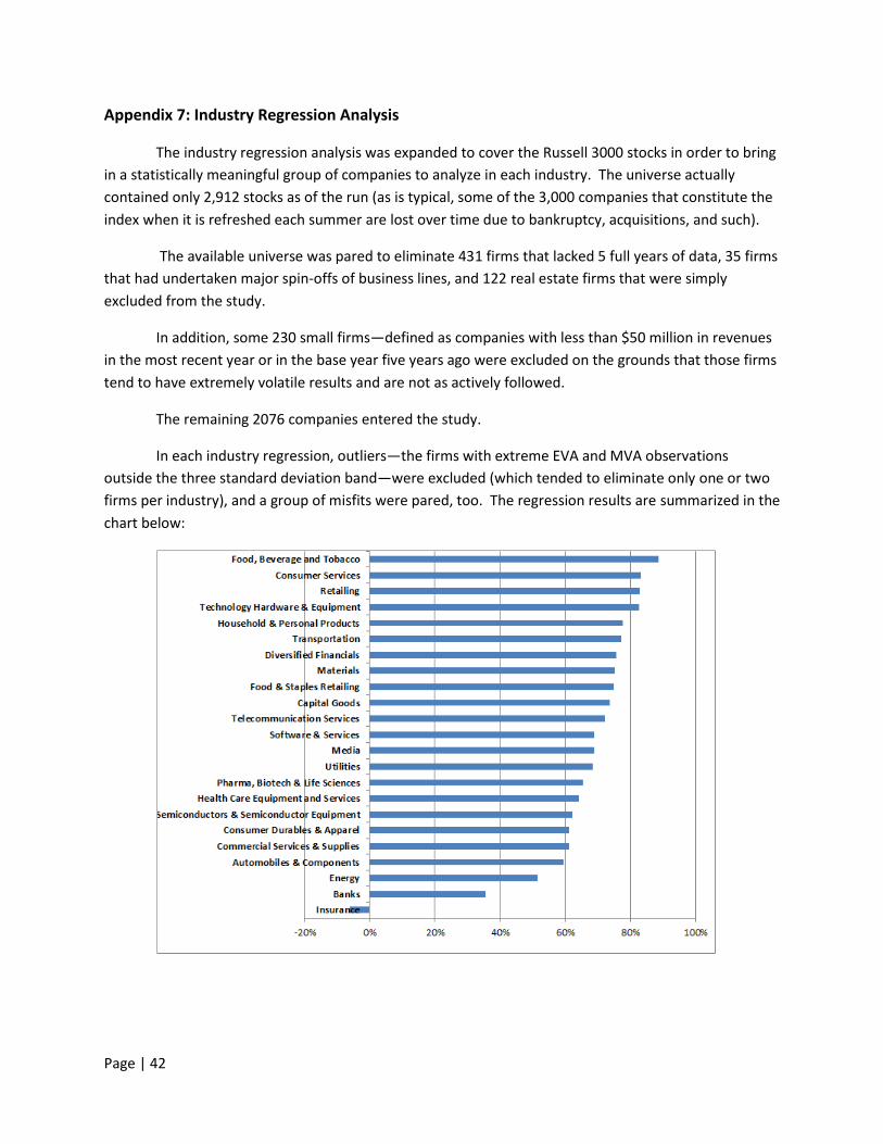
Page | 42

Appendix 7: Industry Regression Analysis

The industry regression analysis was expanded to cover the Russell 3000 stocks in order to bring

in a statistically meaningful group of companies to analyze in each industry. The universe actually

contained only 2,912 stocks as of the run (as is typical, some of the 3,000 companies that constitute the

index when it is refreshed each summer are lost over time due to bankruptcy, acquisitions, and such).

The available universe was pared to eliminate 431 firms that lacked 5 full years of data, 35 firms

that had undertaken major spin-offs of business lines, and 122 real estate firms that were simply

excluded from the study.

In addition, some 230 small firms—defined as companies with less than $50 million in revenues

in the most recent year or in the base year five years ago were excluded on the grounds that those firms

tend to have extremely volatile results and are not as actively followed.

The remaining 2076 companies entered the study.

In each industry regression, outliers—the firms with extreme EVA and MVA observations

outside the three standard deviation band—were excluded (which tended to eliminate only one or two

firms per industry), and a group of misfits were pared, too. The regression results are summarized in the

chart below:

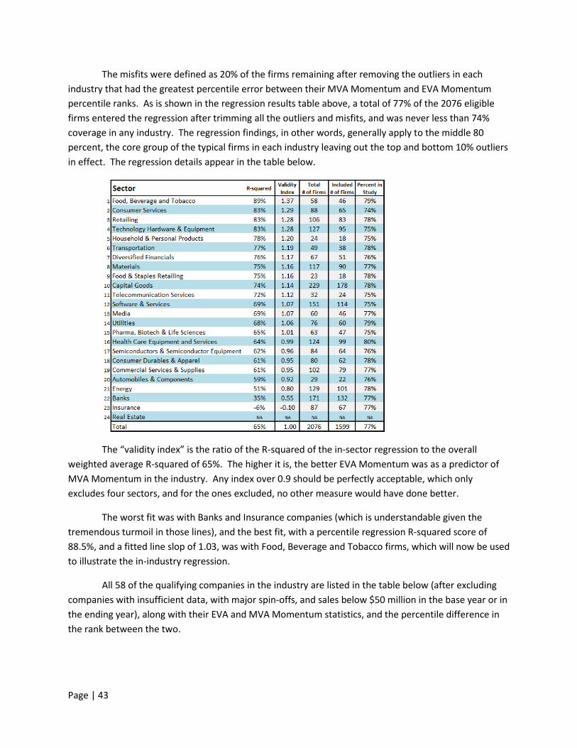
Page | 43

The misfits were defined as 20% of the firms remaining after removing the outliers in each

industry that had the greatest percentile error between their MVA Momentum and EVA Momentum

percentile ranks. As is shown in the regression results table above, a total of 77% of the 2076 eligible

firms entered the regression after trimming all the outliers and misfits, and was never less than 74%

coverage in any industry. The regression findings, in other words, generally apply to the middle 80

percent, the core group of the typical firms in each industry leaving out the top and bottom 10% outliers

in effect. The regression details appear in the table below.

The “validity index” is the ratio of the R-squared of the in-sector regression to the overall

weighted average R-squared of 65%. The higher it is, the better EVA Momentum was as a predictor of

MVA Momentum in the industry. Any index over 0.9 should be perfectly acceptable, which only

excludes four sectors, and for the ones excluded, no other measure would have done better.

The worst fit was with Banks and Insurance companies (which is understandable given the

tremendous turmoil in those lines), and the best fit, with a percentile regression R-squared score of

88.5%, and a fitted line slop of 1.03, was with Food, Beverage and Tobacco firms, which will now be used

to illustrate the in-industry regression.

All 58 of the qualifying companies in the industry are listed in the table below (after excluding

companies with insufficient data, with major spin-offs, and sales below $50 million in the base year or in

the ending year), along with their EVA and MVA Momentum statistics, and the percentile difference in

the rank between the two.

Page | 44

The charts below illustrate the typical progression of the regressions as they proceeded through

the statistical analysis gristmill. The first included all of the 58 eligible firms shown above. The second

excluded the one outlier, Green Mountain Coffee, which racked up stupendous EVA and MVA. It was a

highly EVA/MVA aligned company, and dropping it reduced the R-squared materially. It is removed,

though, because one extreme observation should not inflate the results for the group (excluding it

dropped the R-squared by far more in the raw variable regression, which is an indication of why the

percentile rank order regression is fundamentally more stable and meaningful). The third regression

eliminated 20% of the remaining firms, i.e., 12 of the 57 companies, that had the least fit between their

EVA Momentum and their MVA Momentum in order to isolate the fundamental ability of EVA to track

with MVA for the core firms in the industry (the same procedure was applied in all industries, so that the

R-Squared’s can be compared for an indication of the relative strength of the relationships). The final

result is a near perfect alignment between EVA Momentum and MVA Momentum and TSR.

Page | 45

All 58 Eligible Companies

57 Companies, Excluding the One Outlier (Green Mountain)

45 Companies, Excluding 1 Outlier and the 12 largest misfits

Page | 46

Appendix 8: Simulating TIR

Our research has shown that the underlying determinants of TSR are TIR, which is the total

return earned in the business, with an overlay for leverage, and that TIR in turn comes chiefly from

earning EVA and increasing it as the best proxy for increasing MVA, the wealth of the owners. Let’s now

put that simple formula through its paces to see how shareholder returns should respond to changes in

corporate performance.

To begin, suppose a company is just breaking even on EVA and is not expected to improve it. In

that case, its MVA is zero and is not expected to increase, because its EVA is zero and not expected to

increase. In short, the firm’s market value should track along with the book value of its capital, and its

TIR is reduced to just the capital charge yield on its market value, as follows:

TIR = (Capital Charge + EVA + ΔMVA)/V0 = (Capital Charge + $0 + $0 )/V0 = (Cost of Capital × Capital + $0 + $0)/Capital = Cost of Capital

Since the firm’s market value matches the capital base in this case, the capital charge delivers a

cost-of-capital return on the value. TIR equals the cost of capital, every year, as expected. This is the

epitome of breaking even, and the classic base case.

Now suppose the company emits a one-time unexpected EVA uptick that has no impact on

expected future EVA and so none on its MVA or market value as well. Then the investor return that year

will increase by the one-time EVA uptick, but no more, and thereafter it will settle right back to the cost

of capital. Nonrecurring profits pay a one-time return dividend but just don’t move the market. There’s

an important message there. Managers should avoid spending a lot of time on generating one-time

gains since the market will assign them a multiple of one, then none.

Now suppose the firm’s EVA rises and investors consider the improvement permanent. The

firm’s MVA increases to incorporate the present value of the increase in EVA projected as a never-

ending perpetuity. The return soars whenever investors are first convinced this will happen. Depending

on the cost of capital, the MVA increase could be 7 to 20 times the increase in annual EVA.

Finally, suppose that investors not only expect the increase in EVA to be permanent, but they

also believe that management has positioned the company to continue increasing EVA for some time. In

this case, the firm’s MVA is turbocharged, as both EVA and future EVA growth rev up. The investor

return skyrockets when the long-run EVA trajectory is revised and impounded into the share price.

The bad news is that, after such a run-up, TIR will be based off a much higher market value. To

just earn the expected cost of capital and produce even just a zero excess return, the company will need

to continue to increase its EVA and hike up its MVA year over year just to stay on track with

expectations. But that is the way markets work. And it is another reason why it is sensible for ISS to

focus on TSR over longer horizons, like over 5 years, and why it is helpful to implement incentive plans

Page | 47

that reward managers not only for increasing the stock price but also for actually delivering the EVA

profit growth the market is expecting.