why don’t we agree? studying inﬂuenza with rna interference€¦ · michael newton uw madison...

Michael NewtonUW Madison

Why don’t we agree? Studying influenza with RNA interference

Tuesday, July 3, 12

From a project on influenza biology with:

Qiuling HeLin HaoMark CravenPaul Ahlquist

Thanks Christina Kendziorski...Tuesday, July 3, 12

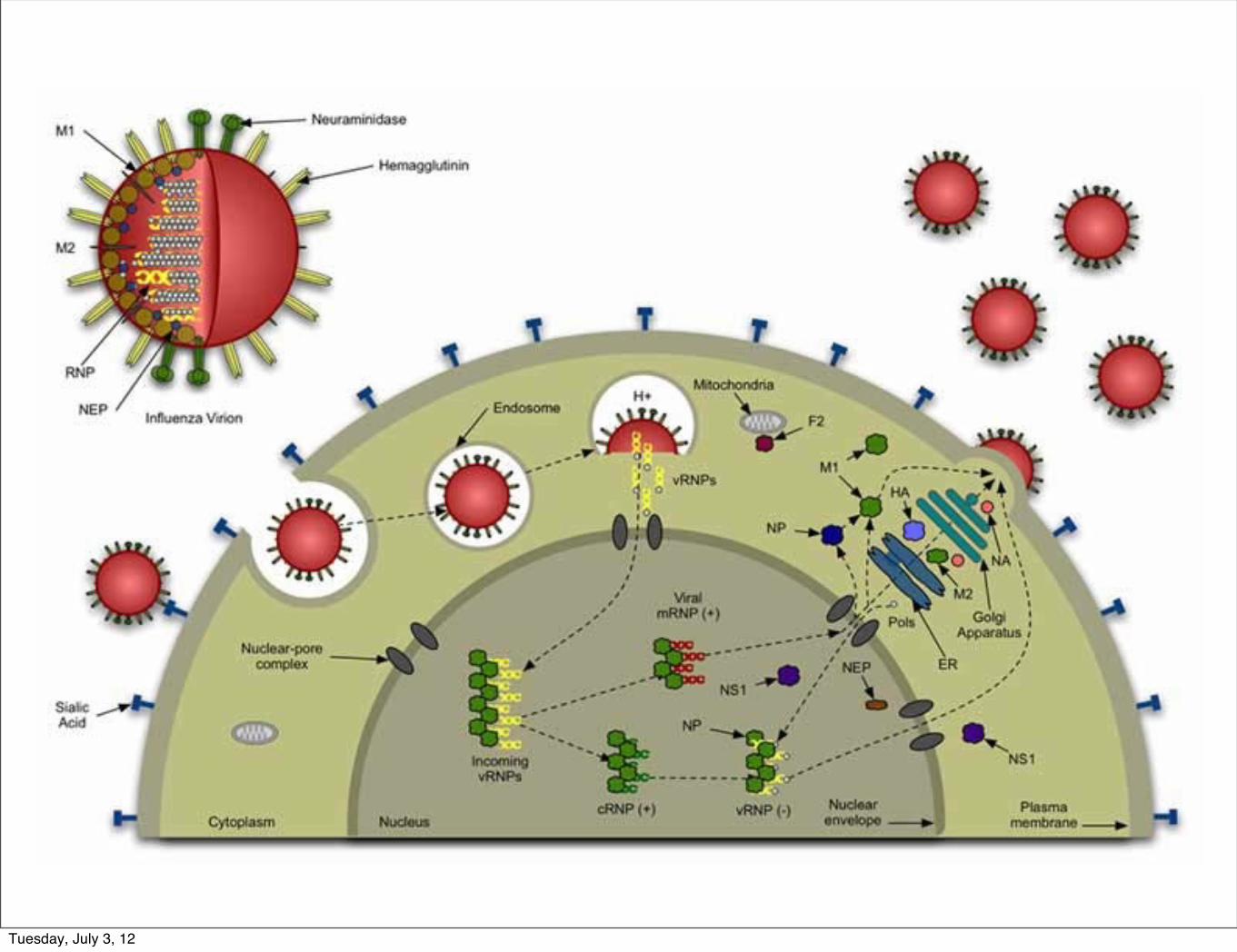
What human genes does influenza virus co-opt during its life cycle?

Tuesday, July 3, 12

a bit about flu

Tuesday, July 3, 12

Tuesday, July 3, 12

RNA interference is a process within living cells that moderates the activity of their genes.

Experimental Method: RNAi

Fire and Mello, 2006, Nobel Prize

Tuesday, July 3, 12

a bit about RNAi

Tuesday, July 3, 12

Kim and Rossi Nature Reviews Genetics 8, 173—184 (March 2007) | doi:10.1038/ nrg2006Tuesday, July 3, 12

Or, more simply, ...

RNA interference =

Tuesday, July 3, 12

Or, more simply, ...

genome-wide...

RNA interference =

Tuesday, July 3, 12

Tuesday, July 3, 12

cell

target gene

expressionlevel

Tuesday, July 3, 12

cell

expressionlevel

add siRNA

target gene

+

Tuesday, July 3, 12

cell

expressionlevel

target gene

Tuesday, July 3, 12

cell

expressionlevel

phenotype of interest changes

target gene

Tuesday, July 3, 12

explain phenotype

Tuesday, July 3, 12

Issues

Tuesday, July 3, 12

gene

expressionlevel

Involvement: gene may not affect phenotype

Tuesday, July 3, 12

involved gene

expressionlevel

Efficiency: knockdown may not be complete

Tuesday, July 3, 12

gene

expressionlevel

Accessibility: something blocks the phenotype

a. no expression in these particular cells

Tuesday, July 3, 12

g1

expressionlevel


b. Redundency/masking

g2

Tuesday, July 3, 12

gene

expressionlevel


c.cytotoxicity

Tuesday, July 3, 12

expressionlevel

Off target effects

target g1

off target g2

not involved

involved

Tuesday, July 3, 12

Measurement error

Tuesday, July 3, 12

Measurement error

non-involved gene

expressionlevel

false positive

Tuesday, July 3, 12

Measurement error

Tuesday, July 3, 12

Measurement error

expressionlevel

involved gene

false negative

Tuesday, July 3, 12

one siRNA

+

knock down

no knock down

Tuesday, July 3, 12

one siRNA

+

on target

off target

on target off targetX Xknock down

no knock down

Tuesday, July 3, 12

one siRNA

+

on target

off target

on target off targetX Xknock down

no knock down

error

error

error

error

X

X

measurement

Tuesday, July 3, 12

15

Meta analysis of four recent studies

2010

2010

2009

2008

A549DE

A549US

U2OS

Human

DL-1 Drosophila

Tuesday, July 3, 12

Data

results (gene lists) from 4 two-stage RNAi studies

Tuesday, July 3, 12

Data


1. detection2. confirmation

Tuesday, July 3, 12

Data


1. detection2. confirmation

DL-1 U2OS A549D E A549U S

Detection Screen 1 1 0 0

Conflrmation Screen 1 0 0 0

Pattern Code 11 10 00 00

e.g., one genestudy

Tuesday, July 3, 12

33

Pattern DL-1 U2OS A549DE A549US # genes

1 0 0 0 0 21,0162 10 0 0 0 803 11 0 0 0 127

… … … … … …6 11 10 0 0 4...

.

.

.

.

.

.

.

.

.

.

.

.

.

.

.79 11 11 11 0 380 11 11 11 10 081 11 11 11 11 1

Total G = 22000

Detec9on and Confirma9on Pa>erns

COPG

Tuesday, July 3, 12

Confirmed by 1 Study

Confirmed by 2 Studies



17

Agreement among studies is low.

Among the 614 genes confirmed by at least one study:

Tuesday, July 3, 12

36

Is the limited overlap due more to false posi9ve or false nega9ve factors?

Tuesday, July 3, 12

37

6.7% average pairwise overlap of confirmed gene lists is significantly higher than expected by chance

Tuesday, July 3, 12

L =Q

⇡ Pn⇡⇡

P⇡ = Prob (gene shows detection/confirmation pattern ⇡ )

n⇡ = #(gene shows detection/confirmation pattern ⇡ )

38

Modeling approach

LikelihoodDL-1 U2OS

A549D

E

A549U

S

1 0 0 0 0 21,016

2 10 0 0 0 80

3 11 0 0 0 127

… … … … … …

6 11 10 0 0 4

.

.

.

.

.

.

.

.

.

.

.

.

.

.

.

.

.

.79 11 11 11 0 3

80 11 11 11 10 0

81 11 11 11 11 1

Total G = 22000

P⇡n⇡⇡

Tuesday, July 3, 12

39

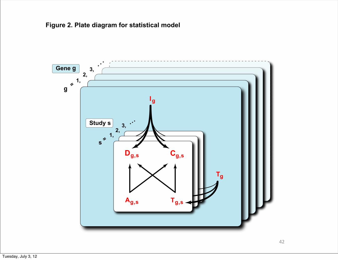
Cg,s = 1 [ gene g confirmed in study s ]

Dg,s = 1 [ gene g detected in study s ]

Ag,s = 1 [ g accessible in s ]

Ig = 1 [ g involved in flu ]

Data and latent variables

Tg,s = #{involved, accessible o↵ targets, study s, target g }

Tuesday, July 3, 12

expression

target gene

Detection screen

pool of 4 distinct siRNA’s per target gene

one phenotype call Dg,s

+

Tuesday, July 3, 12

Confirmation screen

Cg,s = 1

"X

k

Cg,s,k � 2

#

expression

target gene

expression

target gene

expression

target gene

expression

target gene

Cg,s,1 Cg,s,2 Cg,s,3 Cg,s,4

++++

Tuesday, July 3, 12

42

��

��

�

��

��

��

��

��

��

��

��

��

��

��

��

Tuesday, July 3, 12

on target knock down model

U1, U2, U3, U4 ⇠iid Uniform(0, 1)

target gene

expressionlevel

Tuesday, July 3, 12



target gene

expressionlevel

U1

Tuesday, July 3, 12



target gene

expressionlevel

Tuesday, July 3, 12



target gene

expressionlevel

U1U2

Tuesday, July 3, 12



target gene

expressionlevel

Tuesday, July 3, 12



target gene

expressionlevel Y

j

Uj

Tuesday, July 3, 12



target gene

expressionlevel Y

j

Uj

Y

j

Uj < �

knock down effect if

threshold parameter

Prob: 1�G4 [log(1/!)]

Tuesday, July 3, 12

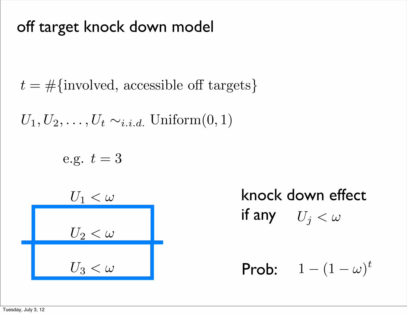
off target knock down model

t = #{involved, accessible o↵ targets}

U1, U2, . . . , Ut ⇠i.i.d. Uniform(0, 1)

e.g. t = 3

U1 < !

U2 < !

U3 < !

knock down effect if any Uj < !

1� (1� !)tProb:

Tuesday, July 3, 12

0.0 0.2 0.4 0.6 0.8 1.00.0

0.2

0.4

0.6

0.8

1.0

ω

Prob

4 hits on target4 hits off target

1�G4 [log(1/!)]

1� (1� !)4

Tuesday, July 3, 12

detection screen:

knock down

no knock down

measurement

+

1� (1� !)t

(1� !)t{G4 [log(1/�)]}ai

1� {G4 [log(1/�)]}ai

�

1� �

↵

1� ↵

Dg,s | Ag,s = a, Ig = i, Tg,s = t

Tuesday, July 3, 12

confirmation screen

Cg,s = 1

"X

k

Cg,s,k � 2

#

expression

target gene

expression

target gene

expression

target gene

expression

target gene

Cg,s,1 Cg,s,2 Cg,s,3 Cg,s,4

++++

Tuesday, July 3, 12

confirmation screen:

knock down

no knock down

measurement

+

�

1� �

↵

1� ↵

1� !⇣1� !

4

⌘t

1�⇣1� !

4

⌘t

Cg,s,k | Ag,s = a, Ig = i, Tg,s = t

1� (1� !)ai

Tuesday, July 3, 12

On the number of off targets per siRNA

• very limited data• libraries overlap among 4 studies

Tuesday, July 3, 12

one target gene

K siRNA’s available to all studies (on average)

siRNA’s

involved off targets

Tg

Tuesday, July 3, 12

one target gene

study s uses 4 siRNA’s

siRNA’s

involved, accessible off targets

Tg,s

x x

Tuesday, July 3, 12

Tg = #{involved o↵-targets, target g }

Tg,s|Tg = t ⇠ Binomial

✓t,4�sK

◆detection

confirmationTg,s,k|Tg,s = t ⇠ Binomial

✓t,1

4

◆

Tg ⇠ Poisson(K✓⌫)

Tuesday, July 3, 12

53

In these terms, the log-likelihood is

L = log Prob(data) =⇧

�

N� logP�, (1)

where pattern probabilities {P�} are defined by a smaller number of parameters through a stochasticmodel of genome-wide RNAi. The model is hierarchical, and is specified using latent random e�ects:

Ig = 1[g is involved in influenza virus replication]

Ag,s = 1[g is accessible in study s ]

Tg = number of involved o�-targets for gene g, relative to a pool of siRNAs

that might be used to target gene g

Tg,s = size of the accessible subset of Tg in study s

Vg,s,k = size of the accessible subset of Tg,s in assay k of secondary screen in study s .

One could alternatively classify the {Ig} as a high-dimensional parameter, but in doing Bayesianinference we would immediately cover it with a prior, so we treat it as a vector of latent factors inthe notation.

A number system-level parameters are used to specify the probability structure of latent vari-ables and observed data; they describe the basic system in terms of rates governing the latentvariables as well as quantities a�ecting false-positive and false-negative detections and confirma-tions:

⌅ = proportion of genome involved in influenza virus replication

� = false positive measurement error

⇥s = false negative measurement error, study s

⇤s = rate at which genes are accessible, study s

� = knockdown e⌅ciency per siRNA

⌃ = average number of o�-targets per siRNA .

The log-likelihood L in (1) is a function of these 12 parameters, which we collect in a vector⌥ = (⌅,�,⇥, ⇤,�, ⌃), where ⇥ = {⇥s}4s=1, ⇤ = {⇤s}4s=1. Thus L = L(⌥). The stochastic model itselfis:

Ig ⇤ Bernoulli(⌅) (2)

Ag,s ⇤ Bernoulli(⇤s)

Tg ⇤ Negative Binomial(⇧,K⌅⌃

K⌅⌃ + ⇧)

Tg,s |[Tg = t] ⇤ Binomial(t,4⇤sK

)

Vg,s,k |[Tg,s = u] ⇤ Binomial(u,1

4)

Dg,s |[Ig = i, Ag,s = a, Tg,s = t] ⇤ Bernoulli⌃1� ⇥s + (�+ ⇥s � 1) [G4,1(� log�)]ai (1� �)t

⌥

Cg,s,k |[Ig = i, Ag,s = a, Vg,s,k = v] ⇤ Bernoulli�1� ⇥s + (�+ ⇥s � 1)(1� �)ai+v

⇥

P (Cg,s = 1|Ig = i, Ag,s = a, Tg,s = u) = P

⇤4⇧

k=1

Cg,s,k ⇥ 2|Ig = i, Ag,s = a, Tg,s = u

⌅.

2

Parameters

Tuesday, July 3, 12

54

In these terms, the log-likelihood is

L = log Prob(data) =⇤

�

N� logP�, (1)

where pattern probabilities {P�} are defined by a smaller number of parameters through a stochasticmodel of genome-wide RNAi. The model is hierarchical, and is specified using latent random e�ects:

Ig = 1[g is involved in influenza virus replication]

Ag,s = 1[g is accessible in study s ]

Tg = number of involved o�-targets for gene g, relative to a pool of siRNAs

that might be used to target gene g

Tg,s = size of the accessible subset of Tg in study s

Vg,s,k = size of the accessible subset of Tg,s in assay k of secondary screen in study s .

One could alternatively classify the {Ig} as a high-dimensional parameter, but in doing Bayesianinference we would immediately cover it with a prior, so we treat it as a vector of latent factors inthe notation.

A number system-level parameters are used to specify the probability structure of latent vari-ables and observed data; they describe the basic system in terms of rates governing the latentvariables as well as quantities a�ecting false-positive and false-negative detections and confirma-tions:

⌅ = proportion of genome involved in influenza virus replication

� = false positive measurement error

⇥s = false negative measurement error, study s

⇤s = rate at which genes are accessible, study s

� = knockdown e⌅ciency per siRNA

⌃ = average number of o�-targets per siRNA .

The log-likelihood L in (1) is a function of these 12 parameters, which we collect in a vector⌥ = (⌅,�,⇥, ⇤,�, ⌃), where ⇥ = {⇥s}4s=1, ⇤ = {⇤s}4s=1. Thus L = L(⌥). The stochastic model itselfis:

Ig ⇥ Bernoulli(⌅)

Ag,s ⇥ Bernoulli(⇤s)

Tg ⇥ Negative Binomial (mean = K⌅⌃, shape = ⇧)

Tg,s |[Tg = t] ⇥ Binomial (t, 4⇤s/K)

Dg,s |[Ig = i, Ag,s = a, Tg,s = t] ⇥ Bernoulli⌅1� ⇥s + (�+ ⇥s � 1) [G4,1(� log�)]ai (1� �)t

⇧

Cg,s,k |[Ig = i, Ag,s = a, Tg,s = t] ⇥ Bernoulli�1� ⇥s + (�+ ⇥s � 1)(1� �)ai(1� �/4)t

⇥

The shape parameter ⇧ = 0.11 is estimated from a predicted distribution of number of o�-targetgenes per dsRNA in a previous study that evaluates the o�-target e�ects of dsRNAs (Kullkarni etal.). G4,1(.) is the c.d.f. of a gamma distribution with shape parameter 4 and scale parameter 1.Another system-level parameter we fix a priori and do not estimate from the data is

K = average number of siRNAs that target a gene.

2

Poisson(K✓⌫)

Tuesday, July 3, 12

P⇡ =X

i,a

P⇡(i, a)

55

studies are heterogeneous, both because they may entail di�erent sets of accessible genes, but alsobecause these accessibility rates (�s) are study specific. (We had considered a single parameter �,but saw substantial improvements when we allow the extra flexibility.) From study to study thedata are not independent, owing to gene specific factors Ig and Tg, which get marginalized in ourlikelihood computation.

The 81 multi-study pattern probabilities {P�} (and thus the log-likelihood L(⌃)) in (1) areobtained as a function of the 8 system-level parameters ⌃ by summing out the discrete-valuedlatent variables. Considering among-gene independence, we focus on a single gene, and sum outvalues of the involvement indicator Ig, the four accessibility indicators Ag,s, and the o�-targetcounts Tg and the four Tg,s. (We model Tg,s’s as subsets of a common Tg to reflect the possibilitythat di�erent studies share siRNAs.) All but the target counts are binary sums; more complicatedis the elimination of the o�-target counts. To investigate this calculation, write the vector a = {as}and the conditional probability of data pattern ⇧ as,

P�(i, a) = P (⇧| Ig = i, {Ag,s}4s=1 = a⇥.

Each multi-study pattern probability P� is computed as a summation of these P�(i, a) over the 25

values of its arguments. The trickier computation is the evaluation of each P�(i, a), which requiresmarginalization of the o�-target counts.

To marginalize the o�-target counts, first recognize that each pattern ⇧ is an intersection offour study-specific patterns ⇧ =

⇤s ⇧s. For example ⇧ = 3111 indicates that the gene is confirmed

and detected in the first study and neither detected nor confirmed in any of the remaining threestudies. The modeling assumptions give

P�(i, a) =�⌅

t=0

P (Tg = t) P�⇧|Ig = i, {Ag,s}4s=1 = a, Tg = t

⇥

=�⌅

t=0

Pois(t)4⇧

s=1

P (⇧s|Ig = i, Ag,s = as, Tg = t)

=�⌅

t=0

Pois(t)4⇧

s=1

t⌅

u=0

Bs(t, u) P (⇧s|Ig = i, Ag,s = as, Tg,s = u)

=�⌅

t=0

Pois(t)4⇧

s=1

t⌅

u=0

Bs(t, u) qs,i,as,u (3)

where Pois(t) = P (Tg = t) = exp{�4⇥⇤}(4⇥⇤)t/t! by the Poisson assumption, Bs(t, u) is theBinomial mass function at u with t trials and success probability �s, and where each contributionqs,i,as,u = P (⇧s|Ig = i, Ag,s = as, Tg,s = u) is computed from the stochastic model (2). Comingback to pattern ⇧ = 3111 for example, the four sub-pattern probabilities are:

q1,i,a1,u = P (Dg,1 = 1|Ig = i, Ag,1 = a1, Tg,1 = u) P (Cg,1 = 1|Ig = i, Ag,1 = a1, Tg,1 = u)



q4,i,a4,u = P (Dg,4 = 0|Ig = i, Ag,4 = a4, Tg,4 = u) P (Cg,4 = 0|Ig = i, Ag,4 = a4, Tg,4 = u) .

A key to simplifying the computation further is to recognize that with respect to the count variableu, each qs,i,as,u is a polynomial in ⌅ = (1 � ⌥)1/4, of degree at most 8u. By careful book-keeping,

3

studies are heterogeneous, both because they may entail di�erent sets of accessible genes, but alsobecause these accessibility rates (�s) are study specific. (We had considered a single parameter �,but saw substantial improvements when we allow the extra flexibility.) From study to study thedata are not independent, owing to gene specific factors Ig and Tg, which get marginalized in ourlikelihood computation.

The 81 multi-study pattern probabilities {P�} (and thus the log-likelihood L(⌃)) in (1) areobtained as a function of the 8 system-level parameters ⌃ by summing out the discrete-valuedlatent variables. Considering among-gene independence, we focus on a single gene, and sum outvalues of the involvement indicator Ig, the four accessibility indicators Ag,s, and the o�-targetcounts Tg and the four Tg,s. (We model Tg,s’s as subsets of a common Tg to reflect the possibilitythat di�erent studies share siRNAs.) All but the target counts are binary sums; more complicatedis the elimination of the o�-target counts. To investigate this calculation, write the vector a = {as}and the conditional probability of data pattern ⇧ as,

P�(i, a) = P (⇧| Ig = i, {Ag,s}4s=1 = a⇥.



To marginalize the o�-target counts, first recognize that each pattern ⇧ is an intersection offour study-specific patterns ⇧ =

⇤s ⇧s. For example ⇧ = 3111 indicates that the gene is confirmed


P�(i, a) =�⌅

t=0

P (Tg = t) P�⇧|Ig = i, {Ag,s}4s=1 = a, Tg = t

⇥

=�⌅

t=0

Pois(t)4⇧

s=1

P (⇧s|Ig = i, Ag,s = as, Tg = t)

=�⌅

t=0

Pois(t)4⇧

s=1

t⌅

u=0

Bs(t, u) P (⇧s|Ig = i, Ag,s = as, Tg,s = u)

=�⌅

t=0

Pois(t)4⇧

s=1

t⌅

u=0

Bs(t, u) qs,i,as,u (3)

where Pois(t) = P (Tg = t) = exp{�4⇥⇤}(4⇥⇤)t/t! by the Poisson assumption, Bs(t, u) is theBinomial mass function at u with t trials and success probability �s, and where each contributionqs,i,as,u = P (⇧s|Ig = i, Ag,s = as, Tg,s = u) is computed from the stochastic model (2). Comingback to pattern ⇧ = 3111 for example, the four sub-pattern probabilities are:




q4,i,a4,u = P (Dg,4 = 0|Ig = i, Ag,4 = a4, Tg,4 = u) P (Cg,4 = 0|Ig = i, Ag,4 = a4, Tg,4 = u) .

A key to simplifying the computation further is to recognize that with respect to the count variableu, each qs,i,as,u is a polynomial in ⌅ = (1 � ⌥)1/4, of degree at most 8u. By careful book-keeping,

3

Calcula9ng pa>ern probabili9es:

Ideally if all 4 studies use the same siRNA library, we would expect K = 4 i.e. there are exactly 4siRNAs targeting every gene as designed; if each study uses a di�erent library, then K = 16 if all li-braries are specific and there is no chance of genes being targeted by siRNAs other than the designedones. K controls the correlation in numbers of o�-targets between studies, i.e. cor(Tg,s,Tg,s0) � 0,as K � ⇥. In our case, we fix K = 12 since the 4 studies of interest use 3 libraries.

A full specification of conditional independence assumptions is in Figure 2. The various mod-eling elements have been introduced to address known features of genome-wide siRNA screening.For example, every additional siRNA applied to an involved gene increases the chance that theharboring cells exhibit a phenotype. The higher the rate of involved genes, the higher the rateof an o�-target phenotype. There is heterogeneity among genes, owing to whether or not theyare involved, and owing to varying amounts of o�-targets associated with their targeting pools ofsiRNAs, but there is among-gene independence in terms of siRNA detection/confirmation. Thestudies are heterogeneous, because they may entail di�erent sets of accessible genes and these ac-cessibility rates (⇥s) are study specific, and also there may be di�erent false negative measurementerrors involved in each study due to individual experimental environment. (We had considered asingle parameter ⇥ and �, but saw substantial improvements when we allow the extra flexibility.)From study to study the data are not independent, owing to gene specific factors Ig and Tg, whichget marginalized in our likelihood computation.

The 81 multi-study pattern probabilities {P�} (and thus the log-likelihood L(⌅)) in (1) areobtained as a function of the 12 system-level parameters ⌅ by summing out the discrete-valuedlatent variables. Considering among-gene independence, we focus on a single gene, and sum outvalues of the involvement indicator Ig, the four accessibility indicators Ag,s, and the o�-targetcounts Tg, the four Tg,s, and the {Vg,s,k}4k=1 for each study. (We model Tg,s’s as subsets of acommon Tg to reflect the possibility that di�erent studies share siRNAs.) All but the target countsare binary sums; more complicated is the elimination of the o�-target counts. To investigate thiscalculation, write the vector a = {as} and the conditional probability of data pattern ⇤ as,

P�(i, a) = P (⇤| Ig = i, {Ag,s}4s=1 = a⇥.



To marginalize the o�-target counts, first recognize that each pattern ⇤ is an intersection offour study-specific patterns ⇤ =

⇤s ⇤s. For example ⇤ = 3111 indicates that the gene is confirmed


P�(i, a) =�⌅

t=0

P (Tg = t) P�⇤|Ig = i, {Ag,s}4s=1 = a, Tg = t

⇥

=�⌅

t=0

NB(t)4⇧

s=1

P (⇤s|Ig = i, Ag,s = as, Tg = t)

=�⌅

t=0

NB(t)4⇧

s=1

t⌅

u=0

Bs(t, u) P (⇤s|Ig = i, Ag,s = as, Tg,s = u)

=�⌅

t=0

NB(t)4⇧

s=1

t⌅

u=0

Bs(t, u) Qs,i,as,u (2)

3

Po(t)

Po(t)

Po(t)

Tuesday, July 3, 12

⇠1 = 1� !

⇠2 = 1� !

4

56

where NB(t) = P (Tg = t) is the point mass of a Negative Binomial distribution with shape pa-rameter ⇤ and mean K⇥⌅, Bs(t, u) is the Binomial mass function at u with t trials and successprobability 4�s

K , and where each contribution Qs,i,as,u = P (⌃s|Ig = i, Ag,s = as, Tg,s = u) is com-puted from the stochastic model (??). Coming back to pattern ⌃ = 3111 for example, the foursub-pattern probabilities are:

Q1,i,a1,u = P (Dg,1 = 1|Ig = i, Ag,1 = a1, Tg,1 = u) P (Cg,1 = 1|Ig = i, Ag,1 = a1, Tg,1 = u)



Q4,i,a4,u = P (Dg,4 = 0|Ig = i, Ag,4 = a4, Tg,4 = u) P (Cg,4 = 0|Ig = i, Ag,4 = a4, Tg,4 = u) .

where

P (Cg,s = 1|Ig = i, Ag,s = as, Tg,s = u) = P

⇤4⇧

k=1

Cg,s,k ⇥ 2|Ig = i, Ag,s = as, Tg,s = u

⌅

A key to simplifying the computation further is to recognize that with respect to the count variableu, each P (Dg,s|Ig, Ag,s, Tg,s) is a polynomial of ⇧1 = 1 � �, and each P (Cg,s|Ig, Ag,s, Tg,s) is apolynomial of ⇧2 = 1 � ⇥

4 . Thus, each Qs,i,as,u is a bivariate polynomial in ⇧1 and ⇧2, of degree atmost u and 4u respectively. By careful book-keeping, we identify coe�cients {bs,p,q} (dependingon system parameters ⌥ and the pattern ⌃) such that

Qs,i,as,u =1⇧

p=0

4⇧

q=0

bs,p,q (⇧p1 ⇧q2)

u

Thus the inner factor of (2)

t⇧

u=0

Bs(t, u) Qs,i,as,u =t⇧

u=0

Bs(t, u)8⇧

j=0

bs,j ⇧uj

=1⇧

p=0

4⇧

q=0

bs,p,q

t⇧

u=0

(⇧p1 ⇧q2)

uBs(t, u)

=1⇧

p=0

4⇧

q=0

bs,p,q

�1� 4�s

K+

4�sK

(⇧p1 ⇧q2)

u⇥t

=1⇧

p=0

4⇧

q=0

bs,p,qes,p,qt,

with the second-last line obtained from the moment generating function of a Binomial variable, andwith es,p,q = 1� 4�s

K + 4�sK (⇧p1 ⇧

q2)

u. Incorporating this back into (2), we obtain for the conditional

4







where


⇤4⇧

k=1


⌅



Qs,i,as,u =1⇧

p=0

4⇧

q=0

bs,p,q (⇧p1 ⇧q2)

u


t⇧

u=0


u=0

Bs(t, u)8⇧

j=0

bs,j ⇧uj

=1⇧

p=0

4⇧

q=0

bs,p,q

t⇧

u=0

(⇧p1 ⇧q2)

uBs(t, u)

=1⇧

p=0

4⇧

q=0

bs,p,q

�1� 4�s

K+

4�sK

(⇧p1 ⇧q2)

u⇥t

=1⇧

p=0

4⇧

q=0

bs,p,qes,p,qt,


K + 4�sK (⇧p1 ⇧

q2)


4

Lemma:

Tuesday, July 3, 12

57







where


⇤4⇧

k=1


⌅



Qs,i,as,u =1⇧

p=0

4⇧

q=0

bs,p,q (⇧p1 ⇧q2)

u


t⇧

u=0


u=0

Bs(t, u)8⇧

j=0

bs,j ⇧uj

=1⇧

p=0

4⇧

q=0

bs,p,q

t⇧

u=0

(⇧p1 ⇧q2)

uBs(t, u)

=1⇧

p=0

4⇧

q=0

bs,p,q

�1� 4�s

K+

4�sK

(⇧p1 ⇧q2)

u⇥t

=1⇧

p=0

4⇧

q=0

bs,p,qes,p,qt,


K + 4�sK (⇧p1 ⇧

q2)


4







where


⇤4⇧

k=1


⌅



Qs,i,as,u =1⇧

p=0

4⇧

q=0

bs,p,q (⇧p1 ⇧q2)

u


t⇧

u=0

Bs(t, u) Qs,i,as,u =1⇧

p=0

4⇧

q=0

bs,p,q

t⇧

u=0

(⇧p1 ⇧q2)

uBs(t, u)

=1⇧

p=0

4⇧

q=0

bs,p,q

�1� 4�s

K+

4�sK

(⇧p1 ⇧q2)

u⇥t

=1⇧

p=0

4⇧

q=0

bs,p,qes,p,qt,


K + 4�sK (⇧p1 ⇧

q2)


4

Tuesday, July 3, 12

58

probability of a pattern given accessibility and involvement:

P�(i, a) =�⌦

t=0

NB(t)4↵

s=1

1⌦

p=0

4⌦

q=0

bs,p,qes,p,qt

=�⌦

t=0

NB(t)1⌦

p1=0

1⌦

p2=0

1⌦

p3=0

1⌦

p4=0

4⌦

q1=0

4⌦

q2=0

4⌦

q3=0

4⌦

q4=0

⇤4↵

s=1

bs,ps,qs

⌅⇤4↵

s=1

es,ps,qs

⌅t

=1⌦

p1=0

1⌦

p2=0

1⌦

p3=0

1⌦

p4=0

4⌦

q1=0

4⌦

q2=0

4⌦

q3=0

4⌦

q4=0

⇤4↵

s=1

bs,ps,qs

⌅ �⌦

t=0

NB(t)

⇤4↵

s=1

es,ps,qs

⌅t

=1⌦

p1=0

1⌦

p2=0

1⌦

p3=0

1⌦

p4=0

4⌦

q1=0

4⌦

q2=0

4⌦

q3=0

4⌦

q4=0

⇤4↵

s=1

bs,ps,qs

⌅⇧

⌥ ⇥

⇥+K�⇤�1� 4

s=1 es,ps,qs

⇥

⌃

� .

where the last line comes from the moment generating function of a Negative Binomial distribution.Finally, the pattern probability P� is obtained by summing over the 25 states of i and a, as indicatedpreviously. This provides a route to computing all 81 multi-study pattern probabilities required forlikelihood evaluation.

5

Po(t)

Po(t)

Po(t)

exp

(�K✓⌫

1�

Y

s

es,ps,qs

!)

Tuesday, July 3, 12

59

• 12 parameters• numerical (nlminb in R) (point es9ma9on)• extensive code tes9ng• MCMC (Bayes under flat prior) (induced parameters and predic9on)

Model fitting

Tuesday, July 3, 12

60

0001

0002

0010

0011

0012

0020

0021

0022

0100

0101

0102

0110

0111

0112

0120

0121

0122

0200

0201

0202

0210

0211

0212

0220

0221

0222

1000

1001

1002

1010

1011

1012

1020

1021

1022

1100

1101

1102

1110

1111

1112

1120

1121

1122

1200

1201

1202

1210

1211

1212

1220

1221

1222

2000

2001

2002

2010

2011

2012

2020

2021

2022

2100

2101

2102

2110

2111

2112

2120

2121

2122

2200

2201

2202

2210

2211

2212

2220

2221

2222

0

50

100

150 data

0001

0002

0010

0011

0012

0020

0021

0022

0100

0101

0102

0110

0111

0112

0120

0121

0122

0200

0201

0202

0210

0211

0212

0220

0221

0222

1000

1001

1002

1010

1011

1012

1020

1021

1022

1100

1101

1102

1110

1111

1112

1120

1121

1122

1200

1201

1202

1210

1211

1212

1220

1221

1222

2000

2001

2002

2010

2011

2012

2020

2021

2022

2100

2101

2102

2110

2111

2112

2120

2121

2122

2200

2201

2202

2210

2211

2212

2220

2221

2222

0.000

0.002

0.004

0.006model fit

0001

0002

0010

0011

0012

0020

0021

0022

0100

0101

0102

0110

0111

0112

0120

0121

0122

0200

0201

0202

0210

0211

0212

0220

0221

0222

1000

1001

1002

1010

1011

1012

1020

1021

1022

1100

1101

1102

1110

1111

1112

1120

1121

1122

1200

1201

1202

1210

1211

1212

1220

1221

1222

2000

2001

2002

2010

2011

2012

2020

2021

2022

2100

2101

2102

2110

2111

2112

2120

2121

2122

2200

2201

2202

2210

2211

2212

2220

2221

2222

0.000.010.020.030.040.050.06 involved

0001

0002

0010

0011

0012

0020

0021

0022

0100

0101

0102

0110

0111

0112

0120

0121

0122

0200

0201

0202

0210

0211

0212

0220

0221

0222

1000

1001

1002

1010

1011

1012

1020

1021

1022

1100

1101

1102

1110

1111

1112

1120

1121

1122

1200

1201

1202

1210

1211

1212

1220

1221

1222

2000

2001

2002

2010

2011

2012

2020

2021

2022

2100

2101

2102

2110

2111

2112

2120

2121

2122

2200

2201

2202

2210

2211

2212

2220

2221

2222

0.00000.00050.00100.00150.00200.00250.0030 non−involved

Tuesday, July 3, 12

61

MCMC looks good

Tuesday, July 3, 12

62

●

●●

●

●

●

● ●

●●

●

●

●

●●

●

●

●●

●

●

●

●

●

●

●●

●

● ●

●

●●

●

● ●

●

●●

●

●

●

●

●●

●

●

●

●

●

●

●

●

●

●

●

●

●

●

●●●

●

● ●

●

●●

●

●●

●

●

●

●

●

●

●

●

●

●

●●

●

●

●

●

●●

●

●

●

●

●

●

●

●

●

●

●

200 220 240 260 280 300 320 340

100

150

200

250

100 simulated data# of Primary Hits

# of

Con

firm

atio

n H

its

Comfirmed vs Detected

●

●

●

●

DL−1

U2OS

A549_DE

A549_US

● DL−1U2OSA549_DEA549_US

Posterior predictive checks look good

Tuesday, July 3, 12

63

Table S3-2: Proportions of dsRNAs with predicted numbers of o�-targets in the DRSC collectionfrom Kulkarni et.al. (2006).

Number of o�-targets 0 1 2� 10 11� 50 51� 100 101+Proportion of dsRNAs (%) 61.21 18.96 13.11 3.04 0.91 2.77

Table S3-3: Estimated parameters and 95% credible intervals from Negative Binomial model atk = 0.110 and Poisson model.

Model Negative Binomial PoissonParameter Point Estimate 95% C.I. Point Estimate 95% C.I.

⇤̂ 0.118 (0.089, 0.150) 0.120 (0.092 0.152)⇥̂ : DL� 1 0.065 (0.047, 0.084) 0.065 (0.049 0.083)⇥̂ : U2OS 0.058 (0.042, 0.076) 0.058 (0.044 0.074)

⇥̂ : A549DE 0.076 (0.054, 0.096) 0.076 (0.057 0.097)⇥̂ : A549US 0.091 (0.068, 0.115) 0.091 (0.069 0.114)

�̂ 0.004 (0.003, 0.004) 0.003 (0.003 0.004)⌅̂ 0.016 (0.000, 0.145) 0.011 (0.000 0.056)⇧̂ 0.685 (0.602, 0.955) 0.676 (0.602 0.859)

Table S3-4: Estimated parameters by four ways of leaving out one study.

Leave out ⇤̂ ⇥̂ : DL� 1 ⇥̂ : U2OS ⇥̂ : A549DE ⇥̂ : A549US �̂ ⌅̂ ⇧̂DL-1 0.093 - 0.070 0.091 0.112 0.004 0.017 0.741U2OS 0.113 0.071 - 0.082 0.065 0.004 0.020 0.649

A549DE 0.181 0.040 0.034 - 0.056 0.004 0.021 0.855A549US 0.098 0.079 0.110 0.092 - 0.003 0.018 0.693

Table S3-5: Predicted number of extra genes confirmed by a 4th study based on modeling the otherthree studies.

Leave Out Predicted Additional 95% Prediction Interval Observed AdditionalDL-1 133 (76, 207) 136U2OS 128 (75, 199) 114A549US 144 (89, 212) 188A549DE 156 (80, 284) 131

8

Cross validation

Tuesday, July 3, 12

64

MLE MEAN a b MLE+✓ 0.128 0.128 0.102 0.160 0.223↵ 0.003 0.003 0.002 0.004 0.000�1 0.083 0.164 0.010 0.337 0.298�2 0.340 0.400 0.266 0.500 0.404�3 0.312 0.375 0.240 0.474 0.336�4 0.038 0.125 0.007 0.277 0.208�1 0.063 0.072 0.049 0.101 0.069�2 0.094 0.107 0.073 0.147 0.086�3 0.113 0.127 0.088 0.169 0.008�4 0.084 0.095 0.068 0.129 0.076! 0.809 0.902 0.751 0.996 0.678⌫ 0.000 0.006 0.000 0.020 0.000

Point estimates

Tuesday, July 3, 12

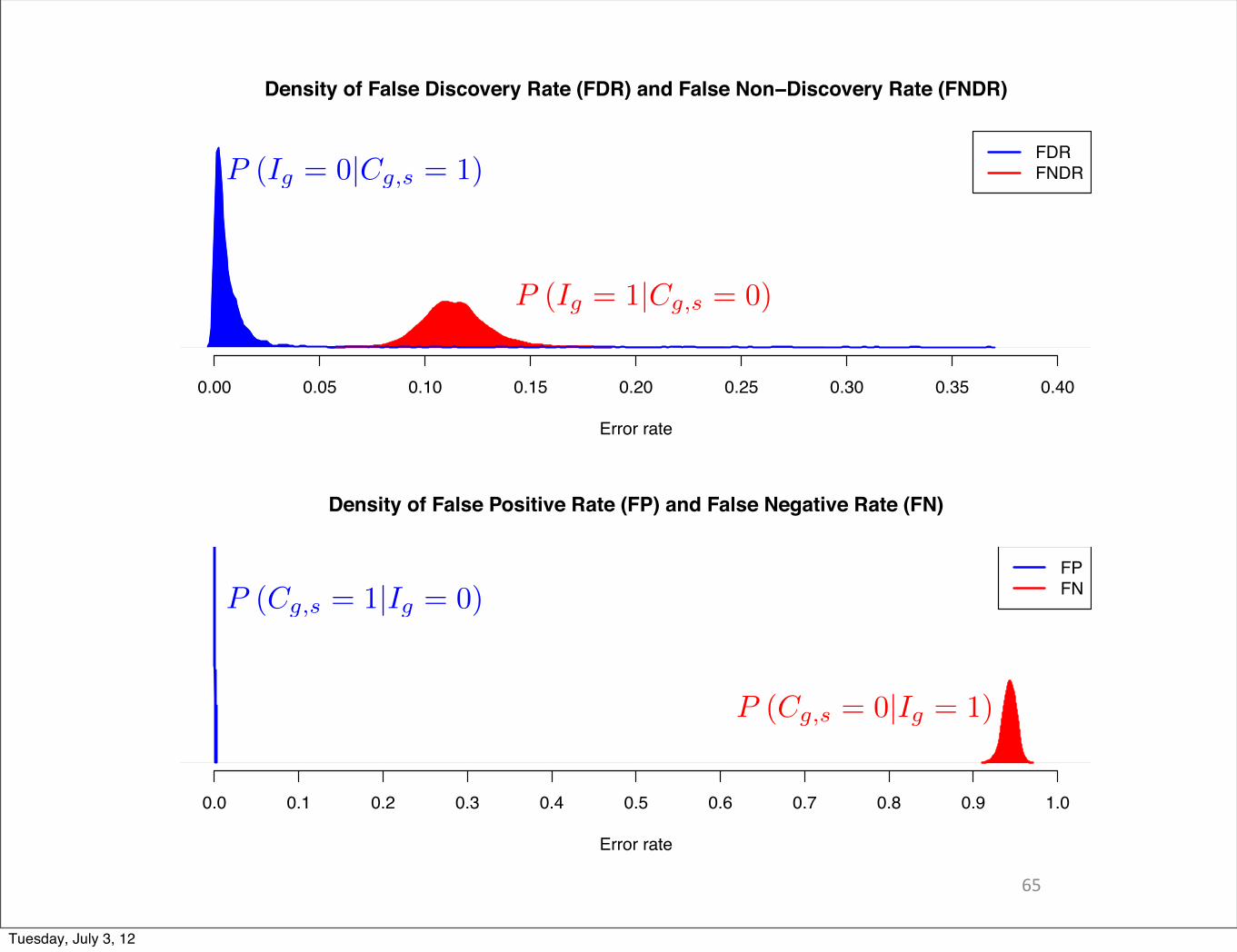
P (Cg,s = 1|Ig = 0)

P (Cg,s = 0|Ig = 1)

P (Ig = 1|Cg,s = 0)

P (Ig = 0|Cg,s = 1)

65

Density of False Discovery Rate (FDR) and False Non−Discovery Rate (FNDR)

Error rate

0.00 0.05 0.10 0.15 0.20 0.25 0.30 0.35 0.40

FDRFNDR

Density of False Positive Rate (FP) and False Negative Rate (FN)

Error rate

0.0 0.1 0.2 0.3 0.4 0.5 0.6 0.7 0.8 0.9 1.0

FPFN

Tuesday, July 3, 12

66

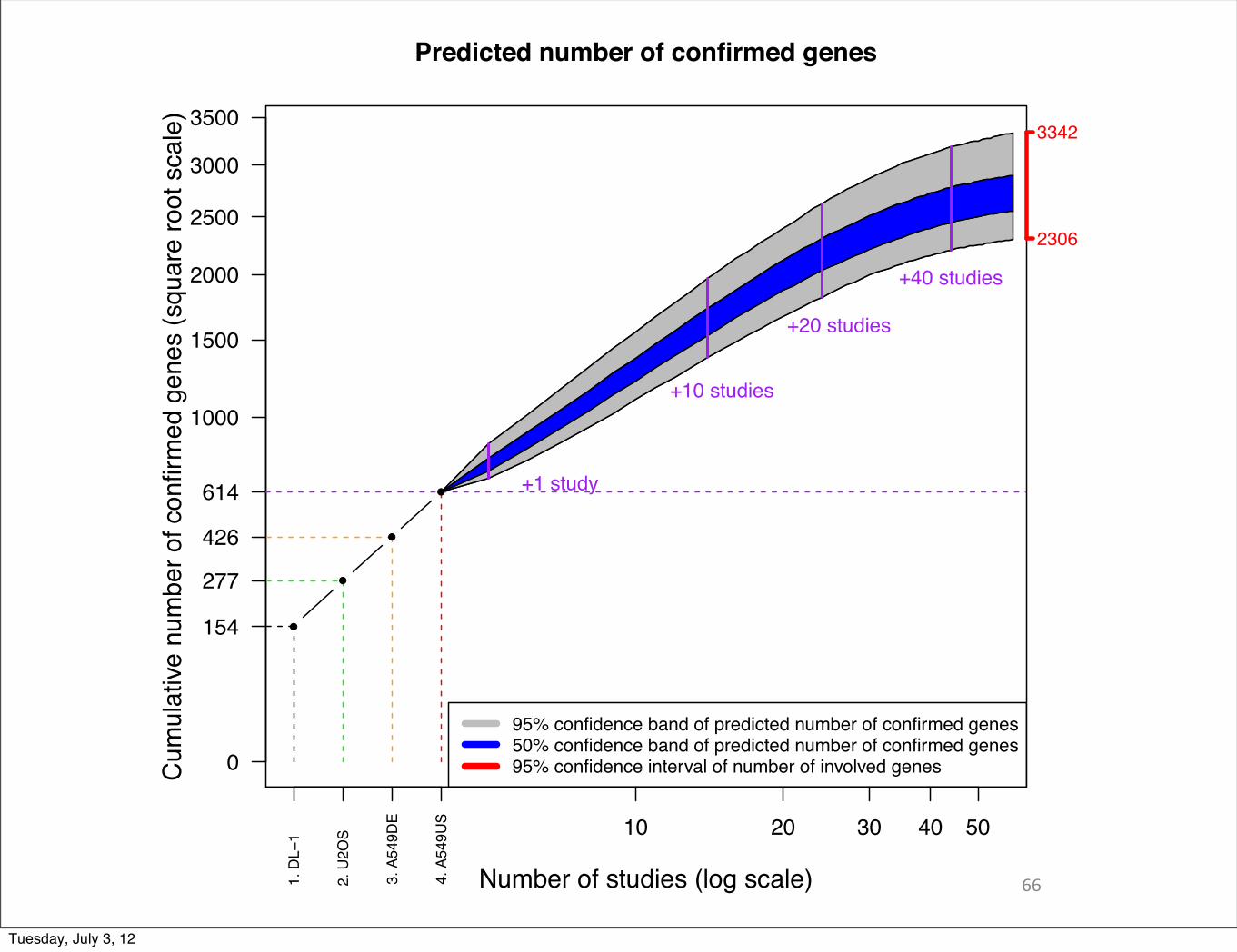
Predicted number of confirmed genes

Number of studies (log scale)

Cum

ulat

ive n

umbe

r of c

onfir

med

gen

es (s

quar

e ro

ot s

cale

)

0

154

277

426

614

1000

1500

2000

2500

3000

3500

10 20 30 40 50

1. D

L−1

2. U

2OS

3. A

549D

E

4. A

549U

S

2306

3342

●

●

●

●

95% confidence band of predicted number of confirmed genes50% confidence band of predicted number of confirmed genes95% confidence interval of number of involved genes

+1 study

+10 studies

+20 studies

+40 studies

Tuesday, July 3, 12

Kulkarni et al. 2006, Nat. Meth.

- computational predictions- overestimate

What about low estimated off target rate ??

Tuesday, July 3, 12

68

probability of a pattern given accessibility and involvement:

P�(i, a) =�⌦

t=0

NB(t)4↵

s=1

1⌦

p=0

4⌦

q=0

bs,p,qes,p,qt

=�⌦

t=0

NB(t)1⌦

p1=0

1⌦

p2=0

1⌦

p3=0

1⌦

p4=0

4⌦

q1=0

4⌦

q2=0

4⌦

q3=0

4⌦

q4=0

⇤4↵

s=1

bs,ps,qs

⌅⇤4↵

s=1

es,ps,qs

⌅t

=1⌦

p1=0

1⌦

p2=0

1⌦

p3=0

1⌦

p4=0

4⌦

q1=0

4⌦

q2=0

4⌦

q3=0

4⌦

q4=0

⇤4↵

s=1

bs,ps,qs

⌅ �⌦

t=0

NB(t)

⇤4↵

s=1

es,ps,qs

⌅t

=1⌦

p1=0

1⌦

p2=0

1⌦

p3=0

1⌦

p4=0

4⌦

q1=0

4⌦

q2=0

4⌦

q3=0

4⌦

q4=0

⇤4↵

s=1

bs,ps,qs

⌅⇧

⌥ ⇥

⇥+K�⇤�1� 4

s=1 es,ps,qs

⇥

⌃

� .

where the last line comes from the moment generating function of a Negative Binomial distribution.Finally, the pattern probability P� is obtained by summing over the 25 states of i and a, as indicatedpreviously. This provides a route to computing all 81 multi-study pattern probabilities required forlikelihood evaluation.

5

Po(t)

Po(t)

Po(t)

exp

(�K✓⌫

1�

Y

s

es,ps,qs

!)

very hard to extend to Nega9ve Binomial

Tuesday, July 3, 12

• large K <==> independent studies• simpler likelihood• separate implementa9on with Nega9ve Binomial gives essen9ally the same fits

69

Sensitivity analysis

Tuesday, July 3, 12

70

0.05 0.10 0.20 0.50 1.00 2.00 5.00

−7600−7400−7200−7000−6800−6600−6400

νpr

ofile

log

likel

ihoo

d

max_[other parameters] log Prob[ data given off−target rate ]

0.05 0.10 0.20 0.50 1.00 2.00 5.00

0.001

0.0050.010

0.0500.100

0.5001.000

ν

dete

ctio

n/co

nfirm

atio

n ra

te

Prob[ detected ]Prob[ confirmed if detected ]four study average

0.05 0.10 0.20 0.50 1.00 2.00 5.000.00

0.05

0.10

0.15

0.20

0.25

0.30

ν

erro

r rat

e

off target rate per siRNA

FDR = Prob[ not involved if confirmed ]FNDR = Prob[ involved if not confirmed ]

Profile analysis

Tuesday, July 3, 12

1. gene-‐level agreement among studies2. func9onal category analysis3. protein interac9on analysis

71

Summary

Tuesday, July 3, 12

Tuesday, July 3, 12

why don’t we agree? studying inﬂuenza with rna interference€¦ · michael newton uw madison...

Documents