Why Has Inflation Been So Unresponsive to Economic Activity in Recent Years?

Robert G. Murphy*

Department of Economics Boston College

Chestnut Hill, MA 02467 murphyro@bc.edu

April 2016

Revised October 2016

Abstract

Standard Phillips curve models relating price inflation to measures of slack in the economy suggest that the

United States should have experienced an episode of deflation during the Great Recession and the

subsequent sluggish recovery. But although inflation reached very low levels, prices continued to rise

rather than fall. More recently, many observers have argued that inflation should have increased as the

unemployment rate declined and labor markets tightened, but inflation has remained below the Federal

Reserve’s policy target. This paper confirms that the slope of the Phillips curve has decreased over recent

decades and is very close to zero today. I modify the Phillips curve to allow its slope to vary continuously

through time drawing on theories of price-setting behavior when prices are costly to adjust and when

information is costly to obtain. I find that adapting the Phillips curve to allow for time-variation in its slope

helps explain inflation before, during, and after the Great Recession.

JEL Classification: E30, E31

Keywords: Inflation, Phillips curve, Great Recession

* I thank Giridaran Subramaniam for expert research assistance. This research was supported in part by a Boston College Research Incentive Grant.

1. Introduction

Standard models relating price inflation to measures of slack in the economy

suggest that the United States should have experienced an episode of deflation during the

Great Recession of 2007 to 2009 and the subsequent sluggish recovery. But although

inflation reached very low levels, prices continued to rise rather than fall. More recently,

many observers have argued that inflation should have increased as the unemployment

rate declined and labor markets tightened, but inflation has remained well below the

Federal Reserve’s policy target.1 These standard Phillips curve models, which

incorporate expectations about future inflation, have in the past performed reasonably

well in forecasting inflation. The failure of these models during the last several years

presents a troubling finding both for economists’ understanding of inflation and for

policymakers’ ability to ensure steady growth and low (but positive) inflation.

These short-run models of inflation build upon the work of Friedman (1968) and

relate inflation to expected inflation and slack in the economy, where slack is often

measured by the gap between unemployment and its natural rate. Most versions of these

models employ past inflation as a proxy for expected inflation, so that the change in

inflation is determined by the gap variable. This “accelerationist” Phillips curve has been

used by numerous authors over the past four decades.2

Recently, several authors have proposed modifications to the standard Phillips

curve that account for the behavior of inflation during and after the Great Recession,

while still maintaining a stable relationship between inflation and the unemployment gap.

These modifications include incorporating inflation expectations that are anchored to the

1 See Friedrich (2014) for an analysis of this “twin puzzle” in the context of overall global inflation. 2 See, for example, Fuhrer (1995), Gordon (1982, 1990), Murphy (1999, 2000), and Staiger et al. (1997). Bernanke (2008) highlights several issues important for analyses of inflation.

2

Federal Reserve’s inflation target, using the short-term unemployment rate rather than the

overall unemployment rate as a measure of economic slack in the economy, and

capturing inflation expectations using survey data.3 By contrast, Murphy (2014)

considers time variation in the relationship between inflation and the unemployment gap

in an otherwise standard accelerationist Phillips curve. He describes how changes in

regional dispersion of economic activity might influence the pricing decisions of firms,

and finds that the resulting time variation in the slope of the Phillips curve can account

for the recent behavior of inflation.

This paper builds on the work of Murphy (2014), extending the time-varying

Phillips curve model of that paper to include more recent data and assessing its ability to

forecast inflation not only since the Great Recession but also over the past several

decades. I modify the Phillips curve to allow its slope to vary continuously through time

drawing on theories of price-setting behavior when prices are costly to adjust and when

information is costly to obtain. I find that adapting the Phillips curve to allow for time-

variation in its slope helps explain inflation before, during, and after the Great Recession.

The paper is organized as follows. Section 2 estimates a standard accelerationist

Phillips curve using data since 1960 and finds a statistically significant weakening in the

responsiveness of inflation to economic activity for sample periods that include data for

years after the Great Recession. Section 3 provides predictions of inflation using this

standard Phillips curve and shows that the model under-predicts inflation in the years

prior to the Great Recession, although it performs very poorly only after 2008. Section 4

3 See the papers by Ball and Mazumder (2015), Coibion and Gorodnichenko (2015), Gordon (2013), Krueger et al (2014), and Watson (2014). Gilchrist et al (2015) highlights defensive pricing by firms facing financial distress as an alternative mechanism attenuating deflationary pressures during the Great Recession.

3

explores time variation in the slope of the Phillips curve and concludes that inflation has

become significantly less responsive to economic activity during the past few decades.

Section 5 considers explanations for why the slope of the Phillips curve varies over time,

highlighting implications of the sticky-price and sticky-information approaches to price

adjustment. These implications suggest that the inflation environment and the extent of

uncertainty about regional economic conditions should influence the slope of the Phillips

curve. I modify the Phillips curve to account for these effects and find that a model in

which the slope varies with the dispersion in regional economic conditions best explains

the path of inflation before, during, and after the Great Recession. The paper concludes

in Section 6 with a review of its findings and suggestions for future research.

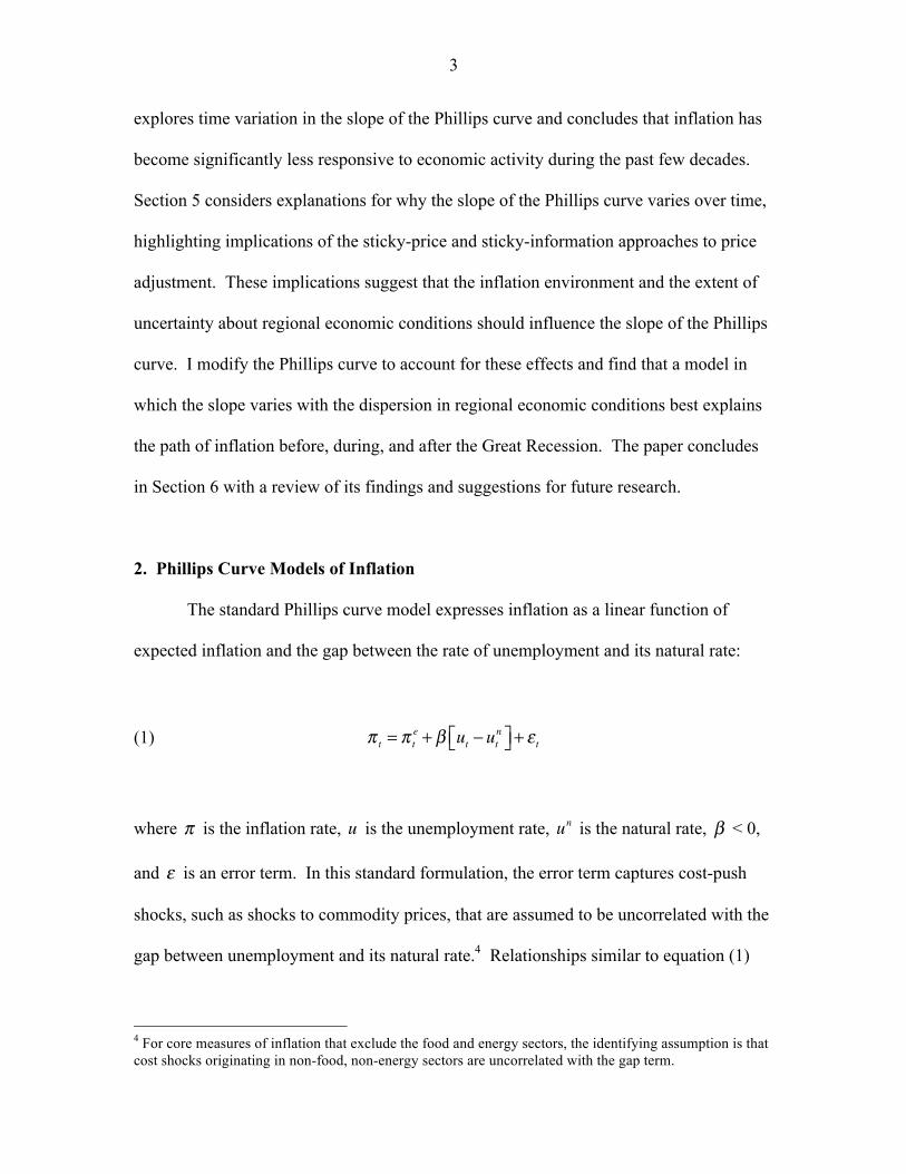
2. Phillips Curve Models of Inflation

The standard Phillips curve model expresses inflation as a linear function of

expected inflation and the gap between the rate of unemployment and its natural rate:

(1) π t = π te + β ut − ut

n⎡⎣ ⎤⎦ + ε t

where π is the inflation rate, u is the unemployment rate, un is the natural rate, β < 0,

and ε is an error term. In this standard formulation, the error term captures cost-push

shocks, such as shocks to commodity prices, that are assumed to be uncorrelated with the

gap between unemployment and its natural rate.4 Relationships similar to equation (1)

4 For core measures of inflation that exclude the food and energy sectors, the identifying assumption is that cost shocks originating in non-food, non-energy sectors are uncorrelated with the gap term.

4

can be derived from microfounded models based on sticky prices or imperfect

information.5

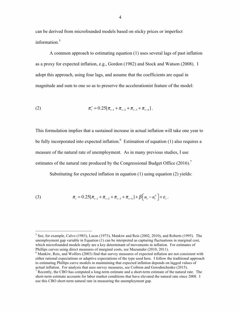
A common approach to estimating equation (1) uses several lags of past inflation

as a proxy for expected inflation, e.g., Gordon (1982) and Stock and Watson (2008). I

adopt this approach, using four lags, and assume that the coefficients are equal in

magnitude and sum to one so as to preserve the accelerationist feature of the model:

(2) π te = 0.25[π t−1 +π t−2 +π t−3 +π t−4 ] .

This formulation implies that a sustained increase in actual inflation will take one year to

be fully incorporated into expected inflation.6 Estimation of equation (1) also requires a

measure of the natural rate of unemployment. As in many previous studies, I use

estimates of the natural rate produced by the Congressional Budget Office (2016).7

Substituting for expected inflation in equation (1) using equation (2) yields:

(3) π t = 0.25[π t−1 +π t−2 +π t−3 +π t−4 ]+ β ut − utn⎡⎣ ⎤⎦ + ε t .

5 See, for example, Calvo (1983), Lucas (1973), Mankiw and Reis (2002, 2010), and Roberts (1995). The unemployment gap variable in Equation (1) can be interpreted as capturing fluctuations in marginal cost, which microfounded models imply are a key determinant of movements in inflation. For estimates of Phillips curves using direct measures of marginal costs, see Mazumder (2010, 2011). 6 Mankiw, Reis, and Wolfers (2003) find that survey measures of expected inflation are not consistent with either rational expectations or adaptive expectations of the type used here. I follow the traditional approach to estimating Phillips curve models in maintaining that expected inflation depends on lagged values of actual inflation. For analysis that uses survey measures, see Coibion and Gorodnichenko (2015). 7 Recently, the CBO has computed a long-term estimate and a short-term estimate of the natural rate. The short-term estimate accounts for labor market conditions that have elevated the natural rate since 2008. I use this CBO short-term natural rate in measuring the unemployment gap.

5

This specification of the Phillips curve captures the accelerationist feature emphasized by

Friedman (1968) whereby a reduction in unemployment below its natural rate leads to a

long-run increase in the rate of inflation.8

To assess whether a standard Phillips curve can explain inflation over the years

since the Great Recession, I estimate equation (3) for the period up to the recession’s start

at the end of 2007 and then for the period through 2015. I begin my sample in 1960,

consistent with the breakpoint highlighted by Barsky (1987) for when inflation changed

from a stationary to an integrated, moving-average process.9

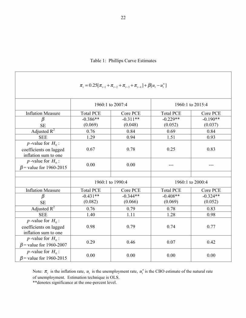
Table 1 presents OLS estimates of equation (3) using quarterly data for inflation

measured using the price index for personal consumption expenditures (PCE). I report

estimates for both total inflation and inflation less food and energy prices (denoted

“core”).10 In all cases, the coefficient on the unemployment gap variable is of the correct

sign (negative) and statistically different from zero at high levels of confidence, and I

cannot reject the restriction that the coefficients on lagged inflation sum to one.

Comparing results for the two time periods in the top panel of Table 1, it is apparent that

the sensitivity of inflation to slack in the economy is much lower when the post 2007 data

are included in the sample than when they are not, with the coefficient dropping by well

over two standard errors for both overall and core inflation.11

8 By contrast, the New Keynesian Phillips curve predicts that inflation is expected to decline when unemployment falls below its natural rate, as Roberts (1995) illustrates. 9 See also Murphy (1986), who examines a break around 1959 in the process determining inflation expectations as measured by the Livingston survey maintained by the Federal Reserve Bank of Philadelphia. 10 All estimates in this paper use data available as of June 2016. I focus on inflation measured using the PCE price index rather than the CPI because the PCE price index encompasses a broader array of consumer purchases and is the measure that the Federal Reserve emphasizes in its policy discussions. Results using CPI inflation are qualitatively similar. 11 P-values for Chow tests reported in Table 1 overwhelmingly reject equality in the two samples.

6

The bottom panel of Table 1 shows results for time periods ending in 1990 and in

2000. Although the point estimates of the coefficient on the unemployment gap are

larger for these samples compared with the sample ending in 2007, we cannot reject at

the five-percent level of significance the hypothesis that they are equal. In contrast, we

can overwhelmingly reject the hypothesis that the coefficients are equal when the sample

ends in 2015. This suggests that equation (3) is not stable across the full sample period of

1960-2015.

3. Inflation Predictions During and After the Great Recession

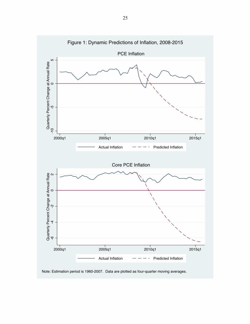
Figure 1 shows forecasts from equation (3) when estimated over the period 1960-

2007 and simulated through the fourth quarter of 2015. These dynamic simulations use

lagged values of predicted inflation to determine expected inflation and actual values of

the unemployment gap.12 Figure 1 presents results for total PCE inflation in the top panel

and for core PCE inflation in the bottom panel. The inflation rates shown in these figures

are four-quarter moving averages, which smooth out fluctuations in the quarterly data.

As shown in Figure 1, the model predicts a period of severe deflation during the years

following the Great Recession for both measures of inflation.

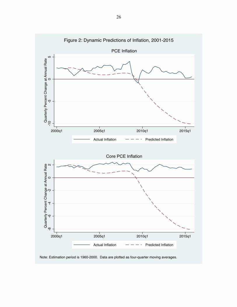
Discussions about monetary policy in the early 2000s focused on worry that the

U.S. economy was on the verge of deflation.13 This suggests considering how well the

Phillips curve performed over the years leading up to the Great Recession. Figure 2

presents forecasts when the estimation sample ends in 2000 and the model is simulated

12 The goal of this paper is to assess how well the Phillips curve explains the recent behavior of inflation. Accordingly, I use actual values of the “exogenous” unemployment gap rather than values that might have been forecast at the end of the estimation period in 2007. 13 See speeches by Federal Reserve Governor Ben Bernanke (2002) and Federal Reserve Chair Alan Greenspan (2002).

7

through the fourth quarter of 2015. As seen in the figure, the model under-predicts both

overall and core inflation starting in 2004 and then shows a sharp decent into deflation

after 2007. These results indicate that the inflation may have become somewhat less

sensitive to demand conditions in the years prior to the Great Recession and that this shift

intensified in the years after.

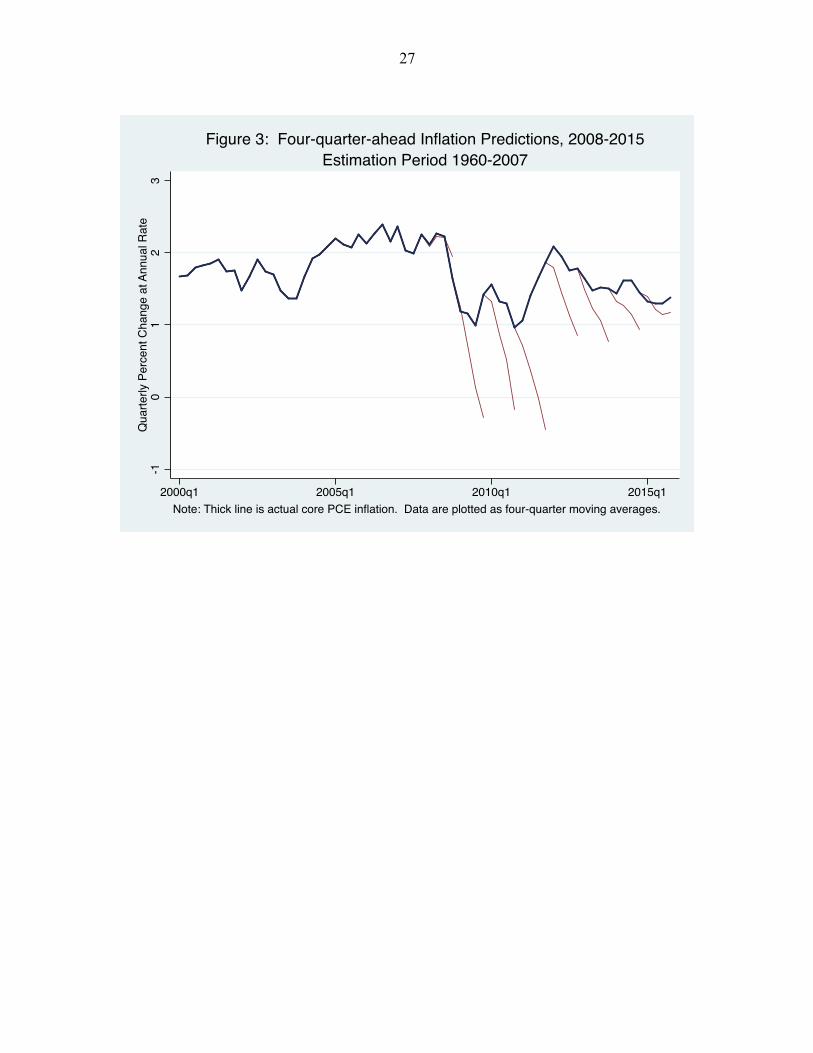
As a further check on these results, Figure 3 shows successive four-quarter

forecasts for core PCE inflation using an estimation period ending in 2007, where the

forecasts start in the first quarter of subsequent years.14 The model predicts inflation well

below its actual value for forecasts starting in years during and immediately following the

Great Recession, although the gap is less for the last few years. Interestingly, the model

does not predict a rise in inflation even as the unemployment rate fell to five percent in

2015, contrary to the views of many observers that tightening labor markets would begin

to push inflation back toward the Federal Reserve’s target of two percent. The reason at

for this, at least in part, is that the CBO estimate of the natural rate of unemployment

used in the model declined along with actual unemployment, so that slack in the economy

has fallen less quickly than the decline in the unemployment rate might suggest.

To gauge whether equation (3) has performed well during earlier periods of time,

Figure 4 provides four-quarter forecasts of inflation over a continually updated sample

for the past 40 years. Specifically, the figure shows successive four-quarter predictions

of core inflation for the model estimated through the end of the previous year. These

predictions are reasonably accurate for most of the period but deteriorate quite obviously

14 Here and in the rest of this paper I focus on core PCE inflation because this measure is the primary one that the Federal Reserve targets and so is most relevant for analysts interested in assessing monetary policy. Results for overall PCE inflation are similar.

8

during the Great Recession and the years following, consistent with inflation becoming

less sensitive to demand conditions than in the past.

4. Time Variation in the Response of Inflation to the Unemployment Gap

A possible explanation for the failure of standard Phillips curve models to explain

the recent behavior of inflation is that the slope coefficient appears to have become much

smaller in recent years. In this section, I confirm a decline in the slope of the Phillips

curve using a rolling regression technique. I also test for an unknown break in the

relationship and find evidence of a shift only when data from years after 2007 are

included in the sample.

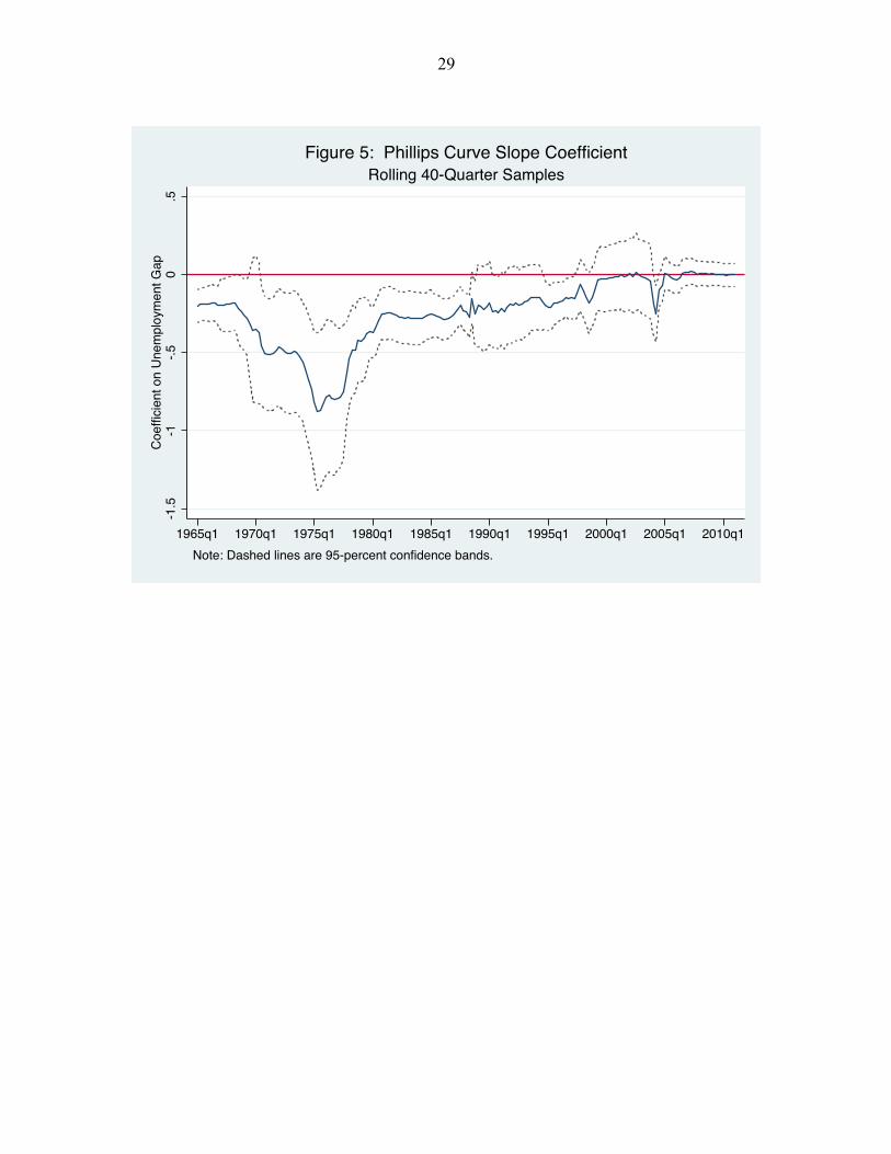
Figure 5 shows estimates of the slope parameter β from equation (3) using

rolling regressions with 10-year windows over the period 1960-2015, centering estimates

at the mid-point of each window. The slope parameter is negative and roughly constant

for most of the 1960s, declines and then rises during the 1970s, plateaus in the 1980s and

first half of the 1990s, and then trends upward through the late 1990s, approaching zero

over the last fifteen years. This pattern is similar to the time variation in Phillips curve

coefficients estimated using advanced time-series techniques in Stock and Watson

(2010a) and Ball and Mazumder (2011).

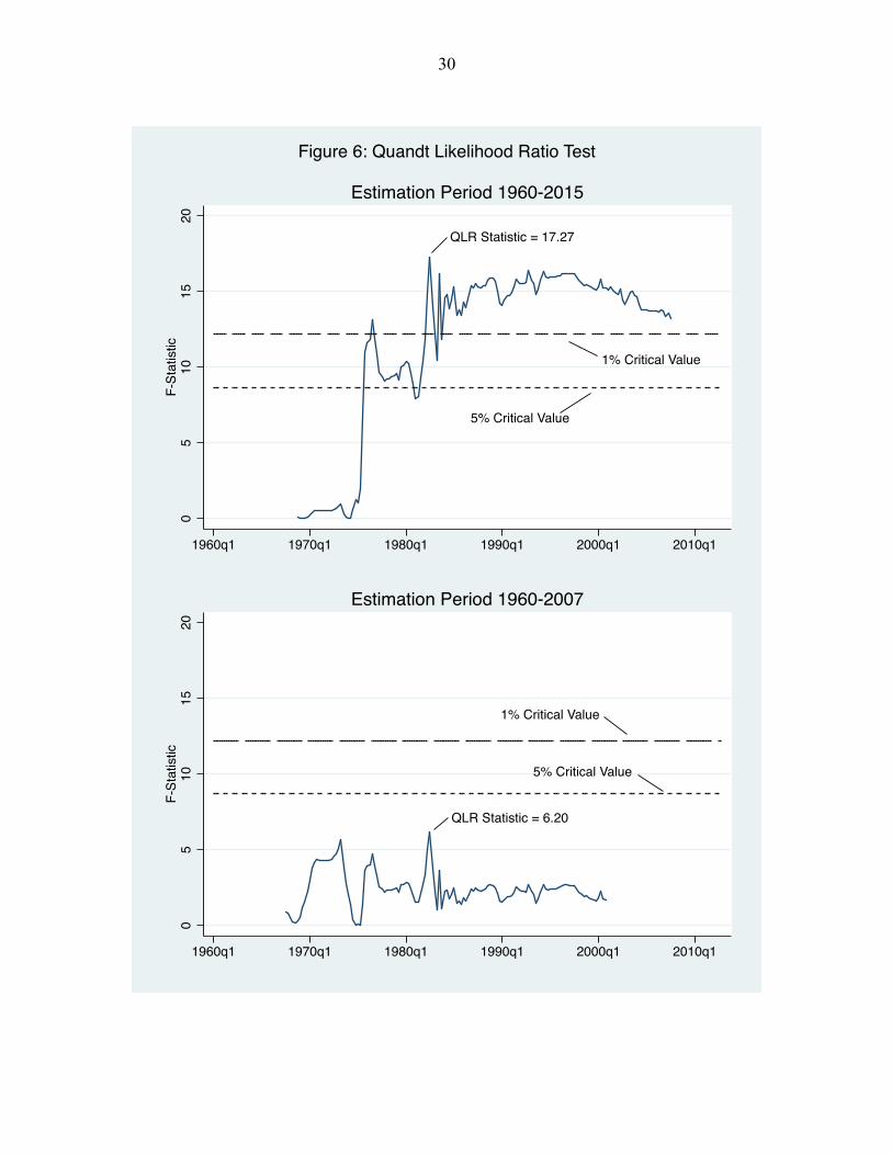
Figure 6 provides results of a Quandt likelihood ratio test for an unknown

structural break in the relationship between inflation and the unemployment gap.15 I can

reject at the one-percent level the hypothesis of no structural break for the sample period

ending in 2015, with the maximum test statistic indicating a break in the early 1980s, as 15 I compute an F-statistic for a Chow test of the null hypothesis of no structural break at each observation over the interior 70 percent of the sample and then chooose the maximum value as the test statistic. Confidence levels for the QLR statistic shown in Figure 6 are from Stock and Watson (2010b), Table 14.6.

9

shown in the top panel. But I cannot reject the hypothesis of no break for the sample

period ending in 2007, as shown in the bottom panel. This suggests that the slope

coefficient in the Phillips curve model is quite sensitive to data for years after 2007,

confirming the results presented in Table 1. Because the maximum value of the QLR

statistic for the full sample is only slightly larger than its value at many other dates, the

test is not very powerful for identifying a single break point. These results are consistent

with a time-varying relationship for the slope coefficient, as shown in Figure 5, and

suggest that directly modeling time-variation of the slope may help explain the recent

behavior of inflation.

5. Accounting for Time Variation in the Phillips Curve

This section considers two explanations for why the Phillips curve’s slope may

vary through time. One explanation assumes prices are costly to adjust and so firms find

it optimal to hold prices constant for some period of time. According to this sticky-price

model of price setting, when the level of inflation is low firms adjust prices less

frequently because low inflation means that fixed prices deviate only gradually from their

optimal values. Similarly, when uncertainty about overall inflation or market demand

conditions is low, the risk that a firm’s fixed price will deviate suddenly from its optimal

value also is low, so firms adjust less frequently because they are less concerned that

fixed prices will be quickly out of line. Since prices are updated less frequently, inflation

will exhibit less responsiveness to shifts in economic slack and the Phillips curve’s slope

coefficient will be smaller in absolute value.16

16 See Ball, Mankiw, and Romer (1988) for an analysis of the sticky-price model’s implications for the slope of the Phillips curve.

10

A second explanation assumes that firms face costs of acquiring information but

are free to adjust prices. Firms set a path for prices and adjust this path only after

updating their information about market demand conditions.17 According to this sticky-

information model of price setting, when uncertainty about market conditions is low,

firms will update their information less frequently, leading to less responsiveness of

inflation to shifts in economic slack and a smaller absolute value for the Phillips curve’s

slope. 18

Because uncertainty about overall inflation affects the benefit of updating

information in addition to the benefit of adjusting prices, inflation variability also will

influence pricing decisions of sticky-information firms as well as sticky-price firms. But

unlike the sticky-price model, the sticky-information model predicts that the average

level of inflation has no effect on the sensitivity of prices to aggregate demand. The

reason for this is that price paths set by firms fully incorporate the average level of

inflation and so inflation has no effect on the frequency of information updates.

As illustrated in Figure 5, the sensitivity of inflation to the unemployment gap

declined during the late 1970s and early 1980s, and then trended lower in the 1990s,

falling close to zero in the 2000s. This suggests that controlling directly for economic

factors influencing the size of the slope coefficient should improve the predictive

performance of the Phillips curve.

To capture uncertainty about market conditions, I develop a measure of dispersion

in economic activity across the United States. In particular, I use the standard deviation

17 See Mankiw and Reis (2007, 2010) for overviews of price-setting models in which information is imperfect. 18 Reis (2006) shows that greater uncertainty about a firm’s market conditions reduces the time between information updates, thereby increasing the responsiveness of prices and inflation to aggregate demand.

11

of growth in state personal income relative to growth in national personal income. The

growth rate is computed as the percent change over the same quarter a year ago. I

calculate the standard deviation for each quarter using data for all fifty states.

Figure 7 plots this regional dispersion variable, computed as a four-quarter

moving average to smooth out quarterly volatility. The dispersion measure is low in the

mid-to-late 1960s, rises and becomes more volatile in the 1970s, and then declines and

becomes less volatile from the mid-1980s onward. This pattern approximates

qualitatively the time-variation seen in Figure 5 for estimates of the slope coefficient for

the Phillips curve.

Figure 8 shows the mean and standard deviation of inflation, calculated on a

rolling basis over 40-quarter intervals.19 These measures of the inflation environment

tend to move together. They are low in the 1960s, increase in the 1970s, decline in the

1980s through the 1990s, and remain low in the 2000s. As with the regional dispersion

variable, the inflation variables qualitatively mimic the time-variation in the slope

coefficient of the Phillips curve, although both of the inflation series are much less

volatile than the regional dispersion series.

To investigate whether changes in the inflation environment and/or the regional

dispersion of economic activity affect the sensitivity of inflation to economic slack, I

modify equation (3) to allow the slope coefficient to vary over time. Specifically, I

estimate versions of the following equation:

19 The estimates shown in Figure 8 are centered at the midpoint of 40-quarter windows. I use estimates from the first and last 40-quarter windows to fill out the first and last 20 quarters of the sample.

12

(4) π t = 0.25[π t−1 +π t−2 +π t−3 +π t−4 ]+ β0[ut − ut

n ] + β1π t[ut − ut

n ]+ β2σ tπ [ut − ut

n ]+ β3σ ty[ut − ut

n ]

where π t and σ tπ are four-quarter moving averages of the mean and standard deviation of

inflation, and σ ty is the four-quarter moving average of the standard deviation of

quarterly state personal income growth around national personal income growth. The

interaction terms capture time variation in the slope coefficient.20

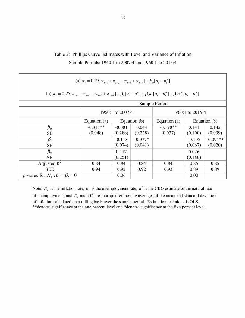
Table 2 reports estimates of two versions of equation (4), first without interaction

terms (as in Table 1) and then with the inflation terms, π t and σ tπ . For the period 1960-

2007, the coefficients on the inflation environment terms (β1 and β2 ) are not statistically

significant either individually or jointly, and the coefficient on the inflation variance term

(β2 ) has an incorrect (positive) sign. For the period 1960-2015, the coefficients are

jointly significant, although the coefficient on the inflation variance term again has an

incorrect (positive) sign. A high degree of collinearity between π t and σ tπ makes the

individual effects hard to distinguish. When the mean of inflation, π t , is entered alone

(second column under version (b)), its coefficient is always statistically significant and of

the correct sign.21 These results provide some weak support for the sticky-price model’s

prediction that the average level of inflation affects the slope of the Phillips curve,

although the positive coefficient on the inflation variance term is at odds with the model’s

prediction. 20 This specification of the Phillips curve permits the slope coefficient to vary over time with the inflation environment and uncertainty about regional economic conditions. The equation is not intended provide a formal test of the sticky-information Phillips curve or the sticky-price Phillips curve. I highlight those pricing models simply to motivate possible reasons why the slope coefficient might vary over time. 21 When the inflation variance term is entered alone (not shown), its coefficient is not statistically significant.

13

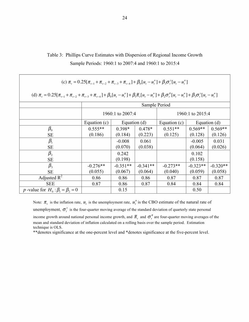
Table 3 reports estimates for two versions of equation (4) that include the regional

dispersion term, σ ty . I present results when the dispersion term is entered alone and in

combination with the inflation environment terms. Again, I provide estimates for the

periods 1960-2007 and 1960-2015.

When I include both the dispersion term and the inflation environment terms (first

column under version (d) in Table 3), the coefficients on the inflation environment terms

(β1 and β2 ) are not statistically significant either individually or jointly, and the

coefficient on the inflation variance term (β2 ) again has an incorrect (positive) sign.

When I include only the mean of inflation with the regional dispersion term (second

column under version (d)), the coefficient on the mean of inflation (β1 ) is not

statistically significant and has an incorrect (positive) sign. The coefficient on the

dispersion term always has the correct (negative) sign, is statistically significant, and is

stable across specifications.22

The results in Tables 2 and 3 strongly suggest that variation over time in the slope

of the Phillips curve is more closely related to regional dispersion of income growth than

to characteristics of inflation. As mentioned above, the average level of inflation should

affect the slope of the Phillips curve in the sticky-price model but not the sticky-

information model. Because the interaction term for the mean of inflation is not

statistically significant when combined with the regional dispersion term, and assuming

that uncertainty about regional economic conditions is captured by the regional

22 When I include the inflation variance term with the regional dispersion term (not shown) and omit the mean inflation term, its coefficient is never statistically significant, while the coefficient on the regional dispersion term is negative and significant.

14

dispersion of income growth, these results are supportive of the sticky-information model

of price setting.

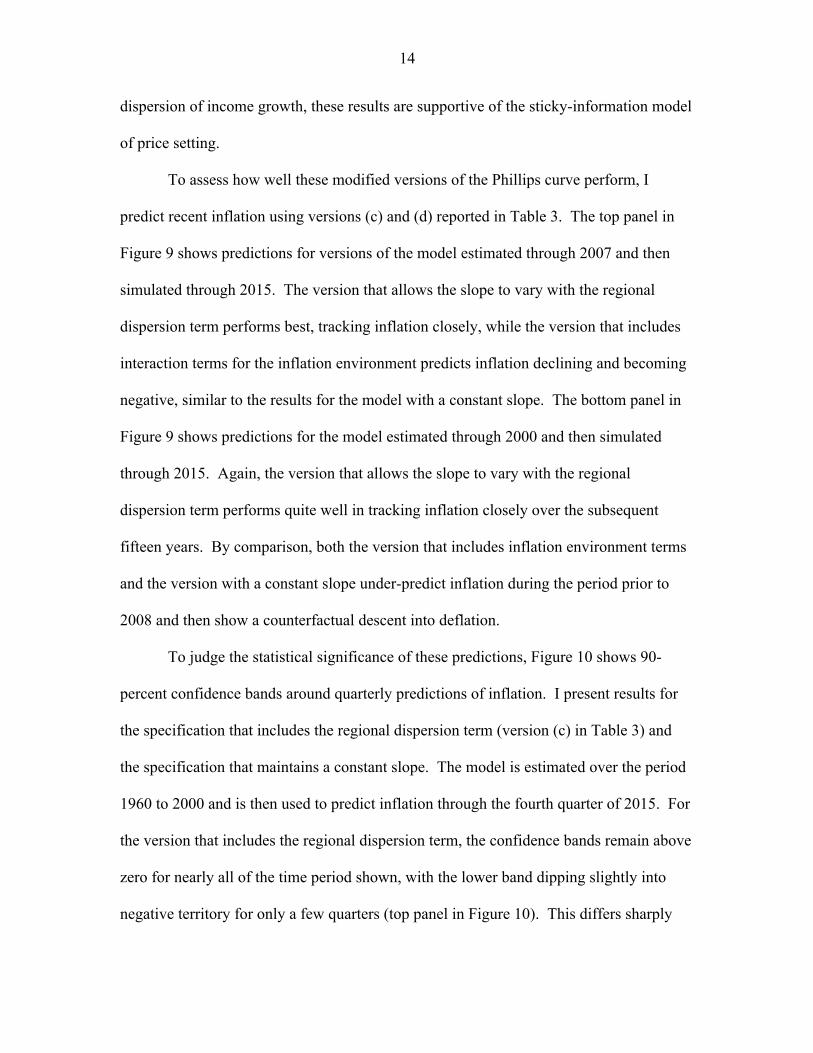
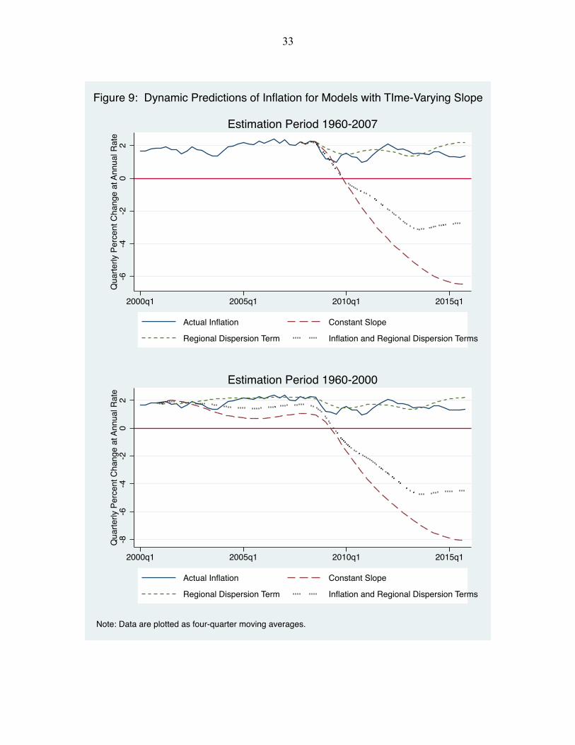
To assess how well these modified versions of the Phillips curve perform, I

predict recent inflation using versions (c) and (d) reported in Table 3. The top panel in

Figure 9 shows predictions for versions of the model estimated through 2007 and then

simulated through 2015. The version that allows the slope to vary with the regional

dispersion term performs best, tracking inflation closely, while the version that includes

interaction terms for the inflation environment predicts inflation declining and becoming

negative, similar to the results for the model with a constant slope. The bottom panel in

Figure 9 shows predictions for the model estimated through 2000 and then simulated

through 2015. Again, the version that allows the slope to vary with the regional

dispersion term performs quite well in tracking inflation closely over the subsequent

fifteen years. By comparison, both the version that includes inflation environment terms

and the version with a constant slope under-predict inflation during the period prior to

2008 and then show a counterfactual descent into deflation.

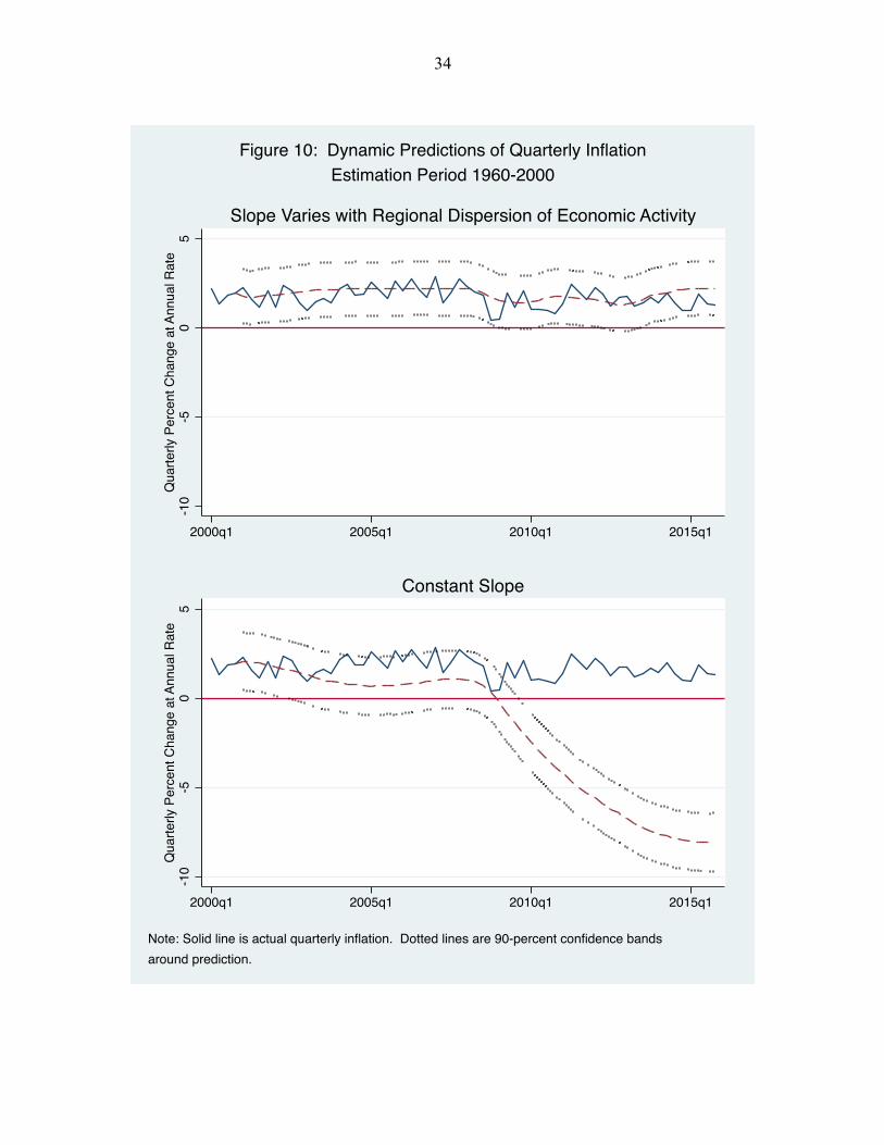
To judge the statistical significance of these predictions, Figure 10 shows 90-

percent confidence bands around quarterly predictions of inflation. I present results for

the specification that includes the regional dispersion term (version (c) in Table 3) and

the specification that maintains a constant slope. The model is estimated over the period

1960 to 2000 and is then used to predict inflation through the fourth quarter of 2015. For

the version that includes the regional dispersion term, the confidence bands remain above

zero for nearly all of the time period shown, with the lower band dipping slightly into

negative territory for only a few quarters (top panel in Figure 10). This differs sharply

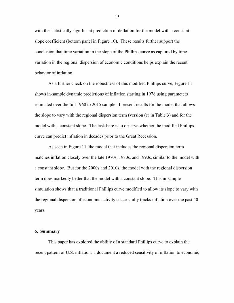
15

with the statistically significant prediction of deflation for the model with a constant

slope coefficient (bottom panel in Figure 10). These results further support the

conclusion that time variation in the slope of the Phillips curve as captured by time

variation in the regional dispersion of economic conditions helps explain the recent

behavior of inflation.

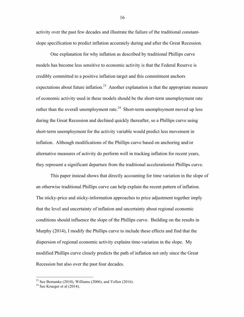
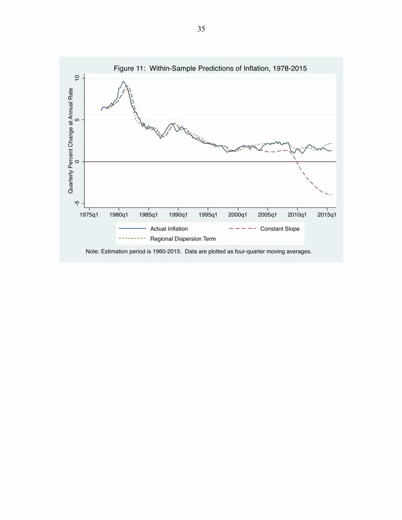
As a further check on the robustness of this modified Phillips curve, Figure 11

shows in-sample dynamic predictions of inflation starting in 1978 using parameters

estimated over the full 1960 to 2015 sample. I present results for the model that allows

the slope to vary with the regional dispersion term (version (c) in Table 3) and for the

model with a constant slope. The task here is to observe whether the modified Phillips

curve can predict inflation in decades prior to the Great Recession.

As seen in Figure 11, the model that includes the regional dispersion term

matches inflation closely over the late 1970s, 1980s, and 1990s, similar to the model with

a constant slope. But for the 2000s and 2010s, the model with the regional dispersion

term does markedly better that the model with a constant slope. This in-sample

simulation shows that a traditional Phillips curve modified to allow its slope to vary with

the regional dispersion of economic activity successfully tracks inflation over the past 40

years.

6. Summary

This paper has explored the ability of a standard Phillips curve to explain the

recent pattern of U.S. inflation. I document a reduced sensitivity of inflation to economic

16

activity over the past few decades and illustrate the failure of the traditional constant-

slope specification to predict inflation accurately during and after the Great Recession.

One explanation for why inflation as described by traditional Phillips curve

models has become less sensitive to economic activity is that the Federal Reserve is

credibly committed to a positive inflation target and this commitment anchors

expectations about future inflation.23 Another explanation is that the appropriate measure

of economic activity used in these models should be the short-term unemployment rate

rather than the overall unemployment rate.24 Short-term unemployment moved up less

during the Great Recession and declined quickly thereafter, so a Phillips curve using

short-term unemployment for the activity variable would predict less movement in

inflation. Although modifications of the Phillips curve based on anchoring and/or

alternative measures of activity do perform well in tracking inflation for recent years,

they represent a significant departure from the traditional accelerationist Phillips curve.

This paper instead shows that directly accounting for time variation in the slope of

an otherwise traditional Phillips curve can help explain the recent pattern of inflation.

The sticky-price and sticky-information approaches to price adjustment together imply

that the level and uncertainty of inflation and uncertainty about regional economic

conditions should influence the slope of the Phillips curve. Building on the results in

Murphy (2014), I modify the Phillips curve to include these effects and find that the

dispersion of regional economic activity explains time-variation in the slope. My

modified Phillips curve closely predicts the path of inflation not only since the Great

Recession but also over the past four decades.

23 See Bernanke (2010), Williams (2006), and Yellen (2016). 24 See Krueger et al (2014).

17

Future research should extend the analysis of this paper to the inflation experience

of other countries in order to assess whether time-variation in the slope of the Phillips

curve is a general phenomenon. Additional work also should compare the predictive

performance of the time-varying Phillips curve model of this paper with the performance

of models relying on anchoring of expectations or alternative measures of economic

activity. Finally, efforts to develop an explicit theoretical framework for how regional

economic conditions influence price adjustment could help further our understanding of

inflation dynamics.

18

References

Ball, L., N. Mankiw, and D. Romer (1988): “The New Keynsesian Economics and the Output-Inflation Trade-off,” Brookings Papers on Economic Activity, 19, 1–82. Ball, L. and S. Mazumder (2011): “Inflation Dynamics and the Great Recession,” Brookings Papers on Economic Activity, Spring 2011, 337–381. Ball, L. and S. Mazumder (2015): “A Phillips Curve with Anchored Expectations and Short-Term Unemployment,” IMF Working Paper WP/15/39, February. Barsky, R. (1987): “The Fisher Hypothesis and the Forecastability and Persistence of Inflation,” Journal of Monetary Economics, 19, 3–24. Bernanke, B. (2002): “Deflation: Making Sure “It” Doesn’t Happen Here,” Remarks before the National Economists Club, Washington, DC, November 21, 2002. Bernanke, B. (2008): “Outstanding Issues in the Analysis of Inflation,” in Understanding Inflation and the Implications for Monetary Policy, ed. by J. Fuhrer, Y. Kodrzycki, J. Little and G. Olivei, MIT Press, 447-456. Bernanke, B. (2010): “The Economic Outlook and Monetary Policy,” Speech at the Federal Reserve Bank of Kansas City Economic Symposium, Jackson Hole, Wyoming. Calvo, G. (1983): “Staggered Prices in a Utility Maximizing Framework,” Journal of Monetary Economics, 12, 383–398. Coibion, O. and Y. Gorodnichenko (2015): “Is the Phillips Curve Alive and Well after All? Inflation Expectations and the Missing Disinflation,” American Economic Journal: Macroeconomics, vol. 7(1), 197-232. Congressional Budget Office (2013): “The Budget and Economic Outlook: Fiscal Years 2013 to 2023,” February 2013, Washington, DC. Friedman, M. (1968): “The Role of Monetary Policy,” American Economic Review, 58, 1–17. Friedrich, C. (2014): “Global Inflation Dynamics in the Post-Crisis Period: What Explains the Twin Puzzle?” Bank of Canada Working Paper 2014-36, August.

19

Fuhrer, J. (1995): “The Phillips Curve is Alive and Well,” New England Economic Review, March/April, 41-56. Gilchrist, S., R. Schoenle, J.W. Sim, and E. Zakrajsek (2015): “Inflation Dynamics During the Financial Crisis,” Finance and Economics Discussion Series 2015-012. Washington: Board of Governors of the Federal Reserve System. Gordon, R. (1982): “Inflation, Flexible Exchange Rates, and the Natural Rate of Unemployment,” in Workers, Jobs, and Inflation, ed. by M. Baily, The Brookings Institution, 89–158. Gordon, R. (1990): “U.S. Inflation, Labor’s Share, and the Natural Rate of Unemployment,” in Economics of Wage Determination, ed. by H. Koenig, Berlin: Springer-Verlag. Gordon, R. (2013): “The Phillips Curve Is Alive and Well: Inflation and the NAIRU during the Slow Recovery.” NBER Working Paper #19390. Greenspan, A. (2002): “Issues for Monetary Policy,” Remarks before the Economic Club of New York, New York City, December 19, 2002. Krueger, A, J. Cramer, and D. Cho (2014): “Are the Long-Term Unemployed on the Margins of the Labor Market?” Brookings Papers on Economic Activity, Spring 2014, 229-280. Lucas, R. (1973): “Some International Evidence on Output-Inflation Tradeoffs,” American Economic Review, 63, 326–34. Mankiw, N. and R. Reis (2002): “Sticky Information Versus Sticky Price: A Proposal to Replace the New Keynesian Phillips Curve,” Quarterly Journal of Economics, 117, 1295– 1328. Mankiw, N. and R. Reis (2007): “Sticky Information in General Equilibrium,” Journal of the European Economic Association, 2, 603-13. Mankiw, N. and R. Reis (2010): “Chapter 5 - Imperfect Information and Aggregate Supply,” in Handbook of Monetary Economics, ed. by B. Friedman and M. Woodford, Elsevier, Volume 3, 183-229.

20

Mankiw, N., R. Reis, and J. Wolfers (2003): “Disagreement about Inflation Expectations,” NBER Working Paper #9796, June 2003. Mazumder, S. (2010): “The New Keynesian Phillips Curve and the Cyclicality of Marginal Cost,” Journal of Macroeconomics, 32, 747-65. Mazumder, S. (2011): “Cost-based Phillips Curve Forecasts of Inflation,” Journal of Macroeconomics, 33, 553-67. Murphy, R. (1986): “The Expectations Theory of the Term Structure: Evidence from Inflation Forecasts,” Journal of Macroeconomics, 8, 423-34. Murphy, R. (1999): “Accounting for the Recent Decline in the NAIRU,” Business Economics, Volume 34. Murphy, R. (2000): “What’s Behind the Decline in the NAIRU?” in The Economic Outlook For 2000, ed. by S. Hymans, University of Michigan, January 2000. Murphy, R. (2014): “Explaining Inflation in the Aftermath of the Great Recession,” Journal of Macroeconomics, 40, 228-44. Reinhart, C. and K. Rogoff (2009): This Time Is Different: Eight Centuries of Financial Folly, Princeton University Press. Reis, R. (2006): “Inattentive Producers,” Review of Economic Studies, 73, 793-821. Roberts, J. (1995): “New Keynesian Economics and the Phillips Curve,” Journal of Money, Credit, and Banking, 27, 975–984. Staiger, D., J. Stock, and M. Watson (1997): “How Precise Are Estimates of the Natural Rate of Unemployment?” in Reducing Inflation: Motivation and Strategy, NBER, 195–246. Stock, J. and M. Watson (2008): “Phillips Curve Inflation Forecasts,” NBER Working Paper, 14322. Stock, J. and M. Watson (2010a): “Modeling Inflation After the Crisis,” NBER Working Paper, 16488. Stock, J. and M. Watson (2010b): Introduction to Econometrics, Prentice Hall.

21

Watson, M. (2014): “Inflation Peristence, the NAIRU, and the Great Recession,” American Economic Review, 104(5), 31-36. Williams, J. (2006): “Inflation Persistence in an Era of Well-anchored Inflation Expectations,” FRBSF Economic Letter, 2006-27. Yellen, J. (2016): “Macroeconomic Research After the Crisis,” Remarks at the 60th Annual Economic Conference, The Elusive ‘Great’ Recovery: Causes and Implications for Future Business Cycle Dynamics, Federal Reserve Bank of Boston, October 14, 2016.

22

Table 1: Phillips Curve Estimates

π t = 0.25[π t−1 +π t−2 +π t−3 +π t−4 ]+ β[ut − utn ]

1960:1 to 2007:4 1960:1 to 2015:4

Inflation Measure Total PCE Core PCE Total PCE Core PCE β

SE -0.386** (0.069)

-0.311** (0.048)

-0.229** (0.052)

-0.190** (0.037)

Adjusted R2 0.76 0.84 0.69 0.84 SEE 1.29 0.94 1.51 0.93

p -value for H0 : coefficients on lagged inflation sum to one

0.67 0.78 0.25 0.83

p -value for H0 : β = value for 1960-2015

0.00 0.00 --- ---

1960:1 to 1990:4 1960:1 to 2000:4

Inflation Measure Total PCE Core PCE Total PCE Core PCE β

SE

-0.431** (0.082)

-0.344** (0.066)

-0.408** (0.069)

-0.324** (0.052)

Adjusted R2 0.76 0.79 0.78 0.83

SEE 1.40 1.11 1.28 0.98 p -value for H0 :

coefficients on lagged inflation sum to one

0.98 0.79 0.74 0.77

p -value for H0 : β = value for 1960-2007 0.29 0.46 0.07 0.42

p -value for H0 : β = value for 1960-2015 0.00 0.00 0.00 0.00

Note: π t is the inflation rate, ut is the unemployment rate, ut

n is the CBO estimate of the natural rate of unemployment. Estimation technique is OLS. **denotes significance at the one-percent level.

23

Table 2: Phillips Curve Estimates with Level and Variance of Inflation

Sample Periods: 1960:1 to 2007:4 and 1960:1 to 2015:4

(a) π t = 0.25[π t−1 +π t−2 +π t−3 +π t−4 ]+ β0[ut − utn ]

(b) π t = 0.25[π t−1 +π t−2 +π t−3 +π t−4 ]+ β0[ut − ut

n ]+ β1π t[ut − utn ]+ β2σ t

π [ut − utn ]

Sample Period

1960:1 to 2007:4 1960:1 to 2015:4

Equation (a) Equation (b) Equation (a) Equation (b) β0 SE

-0.311** (0.048)

-0.001 (0.288)

0.044 (0.228)

-0.190** (0.037)

0.141 (0.100)

0.142 (0.099)

β1 SE

-0.113 (0.074)

-0.077* (0.041) -0.105

(0.067) -0.095** (0.020)

β2 SE

0.117 (0.251) 0.026

(0.180)

Adjusted R2 0.84 0.84 0.84 0.84 0.85 0.85 SEE 0.94 0.92 0.92 0.93 0.89 0.89

p -value for H0 :β1 = β2 = 0 0.06 0.00

Note: π t is the inflation rate, ut is the unemployment rate, utn is the CBO estimate of the natural rate

of unemployment, and π t and σ tπ are four-quarter moving averages of the mean and standard deviation

of inflation calculated on a rolling basis over the sample period. Estimation technique is OLS. **denotes significance at the one-percent level and *denotes significance at the five-percent level.

24

Table 3: Phillips Curve Estimates with Dispersion of Regional Income Growth

Sample Periods: 1960:1 to 2007:4 and 1960:1 to 2015:4

(c) π t = 0.25[π t−1 +π t−2 +π t−3 +π t−4 ]+ β0[ut − utn ]+ β3σ t

y[ut − utn ]

(d) π t = 0.25[π t−1 +π t−2 +π t−3 +π t−4 ]+ β0[ut − ut

n ]+ β1π t[ut − utn ]+ β2σ t

π [ut − utn ]+ β3σ t

y[ut − utn ]

Sample Period

1960:1 to 2007:4 1960:1 to 2015:4

Equation (c) Equation (d) Equation (c) Equation (d) β0 SE

0.555** (0.186)

0.398* (0.184)

0.478* (0.223)

0.551** (0.125)

0.569** (0.128)

0.569** (0.126)

β1 SE

-0.008 (0.070)

0.061 (0.038) -0.005

(0.064) 0.031

(0.026) β2 SE

0.242 (0.198) 0.102

(0.158)

β3 SE

-0.276** (0.055)

-0.351** (0.067)

-0.341** (0.064)

-0.273** (0.040)

-0.323** (0.059)

-0.320** (0.058)

Adjusted R2 0.86 0.86 0.86 0.87 0.87 0.87 SEE 0.87 0.86 0.87 0.84 0.84 0.84

p -value for H0 :β1 = β2 = 0 0.15 0.50 Note: π t is the inflation rate, ut is the unemployment rate, ut

n is the CBO estimate of the natural rate of

unemployment, σ ty is the four-quarter moving average of the standard deviation of quarterly state personal

income growth around national personal income growth, and π t and σ tπ are four-quarter moving averages of the

mean and standard deviation of inflation calculated on a rolling basis over the sample period. Estimation technique is OLS. **denotes significance at the one-percent level and *denotes significance at the five-percent level.

25

-10

-50

5Q

uarte

rly P

erce

nt C

hang

e at

Ann

ual R

ate

2000q1 2005q1 2010q1 2015q1

Actual Inflation Predicted Inflation

PCE Inflation-6

-4-2

02

Qua

rterly

Per

cent

Cha

nge

at A

nnua

l Rat

e

2000q1 2005q1 2010q1 2015q1

Actual Inflation Predicted Inflation

Core PCE Inflation

Note: Estimation period is 1960-2007. Data are plotted as four-quarter moving averages.

Figure 1: Dynamic Predictions of Inflation, 2008-2015

26

-10

-50

5Q

uarte

rly P

erce

nt C

hang

e at

Ann

ual R

ate

2000q1 2005q1 2010q1 2015q1

Actual Inflation Predicted Inflation

PCE Inflation-8

-6-4

-20

2Q

uarte

rly P

erce

nt C

hang

e at

Ann

ual R

ate

2000q1 2005q1 2010q1 2015q1

Actual Inflation Predicted Inflation

Core PCE Inflation

Note: Estimation period is 1960-2000. Data are plotted as four-quarter moving averages.

Figure 2: Dynamic Predictions of Inflation, 2001-2015

27

-10

12

3Q

uarte

rly P

erce

nt C

hang

e at

Ann

ual R

ate

2000q1 2005q1 2010q1 2015q1Note: Thick line is actual core PCE inflation. Data are plotted as four-quarter moving averages.

Estimation Period 1960-2007Figure 3: Four-quarter-ahead Inflation Predictions, 2008-2015

28

02

46

810

Qua

rterly

Per

cent

Cha

nge

at A

nnua

l Rat

e

1975q1 1980q1 1985q1 1990q1 1995q1 2000q1 2005q1 2010q1 2015q1Note: Thick line is actual core PCE inflation. Estimation period begins in 1960. Predictions beginin 1978. Data are plotted as four-quarter moving averages.

Continually Updated SampleFigure 4: Four-quarter-ahead Inflation Predictions, 1978-2015

29

-1.5

-1-.5

0.5

Coe

ffici

ent o

n U

nem

ploy

men

t Gap

1965q1 1970q1 1975q1 1980q1 1985q1 1990q1 1995q1 2000q1 2005q1 2010q1Note: Dashed lines are 95-percent confidence bands.

Rolling 40-Quarter SamplesFigure 5: Phillips Curve Slope Coefficient

30

1% Critical Value

QLR Statistic = 17.27

5% Critical Value

05

1015

20F-

Stat

istic

1960q1 1970q1 1980q1 1990q1 2000q1 2010q1

Estimation Period 1960-2015

QLR Statistic = 6.20

1% Critical Value

5% Critical Value

05

1015

20F-

Stat

istic

1960q1 1970q1 1980q1 1990q1 2000q1 2010q1

Estimation Period 1960-2007

Figure 6: Quandt Likelihood Ratio Test

31

12

34

56

Perc

ent

1960q1 1970q1 1980q1 1990q1 2000q1 2010q1 2020q1Note: Data are 4-quarter moving average of quarterly standard deviation about national average.Growth rate of personal income is computed as percent change over a year ago.

Figure 7: Dispersion of State Personal Income Growth

32

Mean of Inflation

Standard Deviation of Inflation

02

46

8Pe

rcen

t

1960q1 1970q1 1980q1 1990q1 2000q1 2010q1 2020q1Note: Data are 4-quarter moving average of mean and standard deviation of PCE inflation.Mean and standard deviation are computed using 40-quarter rolling samples centered on date shown.

Figure 8: The Inflation Environment

33

-6-4

-20

2Q

uarte

rly P

erce

nt C

hang

e at

Ann

ual R

ate

2000q1 2005q1 2010q1 2015q1

Actual Inflation Constant Slope

Regional Dispersion Term Inflation and Regional Dispersion Terms

Estimation Period 1960-2007-8

-6-4

-20

2Q

uarte

rly P

erce

nt C

hang

e at

Ann

ual R

ate

2000q1 2005q1 2010q1 2015q1

Actual Inflation Constant Slope

Regional Dispersion Term Inflation and Regional Dispersion Terms

Estimation Period 1960-2000

Note: Data are plotted as four-quarter moving averages.

Figure 9: Dynamic Predictions of Inflation for Models with TIme-Varying Slope

34

-10

-50

5Q

uarte

rly P

erce

nt C

hang

e at

Ann

ual R

ate

2000q1 2005q1 2010q1 2015q1

Slope Varies with Regional Dispersion of Economic Activity

-10

-50

5Q

uarte

rly P

erce

nt C

hang

e at

Ann

ual R

ate

2000q1 2005q1 2010q1 2015q1

Constant Slope

Note: Solid line is actual quarterly inflation. Dotted lines are 90-percent confidence bandsaround prediction.

Estimation Period 1960-2000Figure 10: Dynamic Predictions of Quarterly Inflation

35

-50

510

Qua

rterly

Per

cent

Cha

nge

at A

nnua

l Rat

e

1975q1 1980q1 1985q1 1990q1 1995q1 2000q1 2005q1 2010q1 2015q1

Actual Inflation Constant SlopeRegional Dispersion Term

Note: Estimation period is 1960-2015. Data are plotted as four-quarter moving averages.

Figure 11: Within-Sample Predictions of Inflation, 1978-2015