why has inflation been so unresponsive to economic conditions in … pap… · · 2018-03-27why...

Why Has Inflation Been So Unresponsive to Economic Conditions in Recent Years?

Robert G. Murphy*

Department of Economics Boston College

Chestnut Hill, MA 02467 [email protected]

Draft: April 2016

Abstract

Standard models relating price inflation to measures of slack in the economy suggest that the United States

should have experienced an episode of deflation during the Great Recession and the subsequent sluggish

recovery. But although inflation reached very low levels, prices continued to rise rather than fall. More

recently, these standard models suggest inflation should have increased as the unemployment rate declined

and labor markets tightened, but inflation has remained well below the Federal Reserve’s policy target.

Modern Phillips curve models, which incorporate expectations about future inflation, have in the past

performed reasonably well in forecasting inflation. The failure of these models during the last several years

presents a troubling finding both for economists’ understanding of inflation and for policymakers’ ability to

ensure steady growth and low (but positive) inflation. This paper modifies the traditional Phillips curve by

considering two mechanisms through which time-variation in response of inflation to economic conditions

could occur. One mechanism argues that the flexibility of prices varies with the level and variability of

inflation, so a stable low-inflation environment may cause inflation to be less responsive to slack in the

economy. Another mechanism emphasizes increased regional synchronization of the business cycle as a

factor reducing the responsiveness of inflation to slack. The paper considers the extent to which each of

these mechanisms may be important for explaining the recent behavior of inflation.

JEL Classification: E30, E31

Keywords: Inflation, Phillips curve

* Paper prepared for presentation at the International Conference on Economic Modeling (EcoMod2016), Lisbon, Portugal, on July 6-8, 2016. An earlier version of the work presented in this paper appeared in Murphy (2014) under the title, “Explaining Inflation in the Aftermath of the Great Recession.”

1. Introduction

Standard models relating price inflation to measures of slack in the economy

suggest that the United States should have experienced an episode of deflation during the

Great Recession of 2007-09 and the subsequent sluggish recovery. But although inflation

reached very low levels, prices continued to rise rather than fall. More recently, these

standard models suggest inflation should have increased as the unemployment rate

declined and labor markets tightened, but inflation has remained well below the Federal

Reserve’s policy target. Modern Phillips curve models, which incorporate expectations

about future inflation, have in the past performed reasonably well in forecasting inflation.

The failure of these models during the last several presents a troubling finding both for

economists’ understanding of inflation and for policymakers’ ability to ensure steady

growth and low (but positive) inflation.

These standard short-run models of inflation build upon the work of Friedman

(1968) and relate inflation to expected inflation and slack in the economy, where slack is

usually measured by either the gap between unemployment and its natural rate or the gap

between GDP and its potential level. These models often employ past inflation as a

proxy for expected inflation, so that the change in inflation is determined by the gap

variable. This canonical accelerationist Phillips curve has been modified and adapted by

numerous authors over the last several decades.1

In a recent paper, Ball and Mazumder (2011) explore the ability of the Phillips

curve model to explain the behavior of inflation during the Great Recession. They

illustrate how a standard Phillips curve estimated using data since 1960 predicts deflation

1 See, for example, Fuhrer (1995), Gordon (1982, 1990), Murphy (1999, 2000), and Staiger et al. (1997). Bernanke (2008) provides an overview of several key issues for Phillips curve analyses of inflation.

2

over the period 2008 to 2010, although actual inflation remained positive. After

accounting for a recent decline in the slope of the Phillips curve by estimating the model

on data only since 1985, and using median inflation to measure underlying core inflation,

Ball and Mazumder find the model predicts median inflation close to its actual path

through the end of 2010. But with substantial economic slack persisting beyond 2010,

Ball and Mazumder find that the Phillips curve again predicts deflation, unless

expectations about inflation are at least partially anchored to the Federal Reserve’s target

inflation rate.2

This paper revisits the question of why the standard Phillips curve has failed to

accurately predict inflation over the past several years. In particular, I modify the Phillips

curve to allow its slope to vary continuously through time. I consider implications of

price-setting models when prices are costly to adjust and when information is costly to

obtain as reasons for time variation in the Phillips curve’s slope. My analysis is not a

formal test of these price-setting models but instead is an assessment of whether the

models’ implications help improve the ability of the Phillips curve to predict recent

inflation. I find that modifying the Phillips curve to allow continuous time-variation in

its slope greatly improves its ability to explain the recent behavior of inflation.

The paper begins in Section 2 by estimating a standard Phillips curve using data

since 1960 and illustrating its prediction of deflation following the Great Recession. I

also show that the Phillips curve underpredicts inflation in the years leading up to the

Great Recession although it performs very poorly only after 2008. Section 3 explores

time variation in the slope of the Phillips curve and confirms that inflation has become

2 I do not consider the role of anchored expectations in this paper but instead seek to explain the recent behavior of inflation by accounting for time variation in the slope of the Phillips curve.

3

much less responsive to economic activity during the past few decades. Estimates of this

time variation indicate that the slope of the Phillips curve was close to zero in the years

just prior to the Great Recession. I test for an unknown sample breakpoint and find a

significant change in slope for the period after the early 1980s and possibly again during

the early 1990s. I provide predictions for inflation using Phillips curves estimated on

data from only the last few decades, again showing predictions of deflation, albeit less

severe than when estimating over the entire sample. But when I simulate Phillips curves

using slope estimates from the period of the Great Recession, I find they predict inflation

above zero.

Section 4 considers reasons why the slope of the Phillips curve might vary

continuously over time, focusing on implications of the sticky-price and sticky-

information approaches to price adjustment. Under both approaches, uncertainty about

market conditions—which I proxy by the variability of inflation and by the dispersion of

regional economic conditions—will affect the response of inflation to aggregate demand.

Sticky-price models of the type developed by Ball, Mankiw, and Romer (1988) imply a

steeper slope when inflation is volatile rather than stable and when regional conditions

are varied rather than similar because price setters facing fixed costs of adjusting prices

will find it beneficial to change prices more often when uncertainty about aggregate and

region-specific shocks is higher. By changing prices more often, these firms are able to

keep their price closer to its optimal level. Sticky-information models of the sort

presented by Mankiw and Reis (2002) imply a steeper slope when inflation is volatile and

regional conditions are varied because price setters will find it beneficial to update

4

information more often and, accordingly, change price paths more often.3 Changing

price paths more often helps ensure that the firm’s price does not deviate too much from

its optimal path. The two approaches diverge, however, on how the level of inflation

influences the responsiveness of prices to aggregate demand. The sticky-price model

predicts more frequent price changes when average inflation is high (holding constant its

variability) compared to when it is low.4 The sticky-information model, on the other

hand, predicts that average inflation has no effect on the frequency of information

updates because the price paths set by firms fully incorporate the average level of

inflation.

These implications suggest that the inflation environment and the extent of

uncertainty about regional economic conditions should influence the slope of the Phillips

curve. I modify the Phillips curve by introducing proxies to account for these effects and

find that the model in which the slope to varies with uncertainty about regional conditions

can best explain the recent path of inflation. The paper concludes in Section 5 with a

summary of its findings and suggestions for further research.

2. The Phillips Curve Model and Inflation

The standard Phillips curve model relates inflation to expected inflation and the

gap between the rate of unemployment and its natural rate:

(1) π t = π te + β ut − ut

n⎡⎣ ⎤⎦ + ε t

3 Reis (2006) shows that the time between information updates depends inversely on uncertainty about a firm’s market conditions. 4 See Ball, Mankiw, and Romer (1988), who present evidence that the slope of the Phillips curve depends on the level of inflation.

5

where π is the inflation rate, u is the unemployment rate, un is the natural rate, β < 0,

and ε is an error term that is assumed to be uncorrelated with the gap between

unemployment and its natural rate. This identifying assumption treats the disturbance

term as capturing relative price movements such as commodity price shocks that are

assumed to be uncorrelated with the gap variable.5 Relationships similar to equation (1)

are consistent with microfounded models based on sticky prices or imperfect

information.6

A common approach to estimating equation (1) assumes expected inflation is a

function of possibly many lags of past inflation, e.g., Gordon (1982) and Stock and

Watson (2008). I adopt this approach, but limit the lags to four and assume that the

coefficients on the lagged inflation terms are equal in magnitude and sum to one so as to

preserve the accelerationist feature of the model:

(2) π te = 0.25[π t−1 +π t−2 +π t−3 +π t−4 ]

This formulation implies that a sustained increase in actual inflation will take one year to

be fully reflected in expected inflation.7 Estimation of equation (1) also requires a

5 When using core measures of inflation that remove relative price shocks in the food and energy sectors, the identifying assumption is that relative price shocks originating in other sectors are uncorrelated with the gap term. 6 See, for example, Calvo (1983), Roberts (1995), Lucas (1973), Mankiw and Reis (2002, 2010). The gap variable in Equation (1) is intended to broadly capture fluctuations in marginal cost, which microfounded models imply are a key determinant of movements in inflation. For estimates of Phillips curves using more direct measures of marginal costs, see Mazumder (2010, 2011). 7 Mankiw, Reis, and Wolfers (2003) find that survey measures of expected inflation are not consistent with either rational expectations or adaptive expectations of the sort used here. They argue that survey measures exhibit some updating in response to recent news about the macroeconomy. I follow the traditional

6

measure of the natural rate of unemployment. Following previous authors, I use the

estimate of the natural rate produced by the Congressional Budget Office (2013).8

Substituting for expected inflation in equation (1) using equation (2) yields:

(3) π t = 0.25[π t−1 +π t−2 +π t−3 +π t−4 ]+ β ut − utn⎡⎣ ⎤⎦ + ε t

This specification of the Phillips curve captures the accelerationist feature emphasized by

Friedman (1968) in that a reduction in unemployment below its natural rate will result in

a long-run increase in the rate of inflation.9 A variant of this equation uses the gap

between actual real GDP and its potential level expressed as a percentage of potential

GDP rather than the unemployment gap.

To assess whether a standard Phillips curve can explain the process for inflation

following the onset of the Great Recession, I estimate equation (3) for the period up to its

start at the end of 2007. I begin my sample in 1960, which has been identified by Barsky

(1987) as a breakpoint when inflation changed from a stationary to an integrated, moving

average process.10

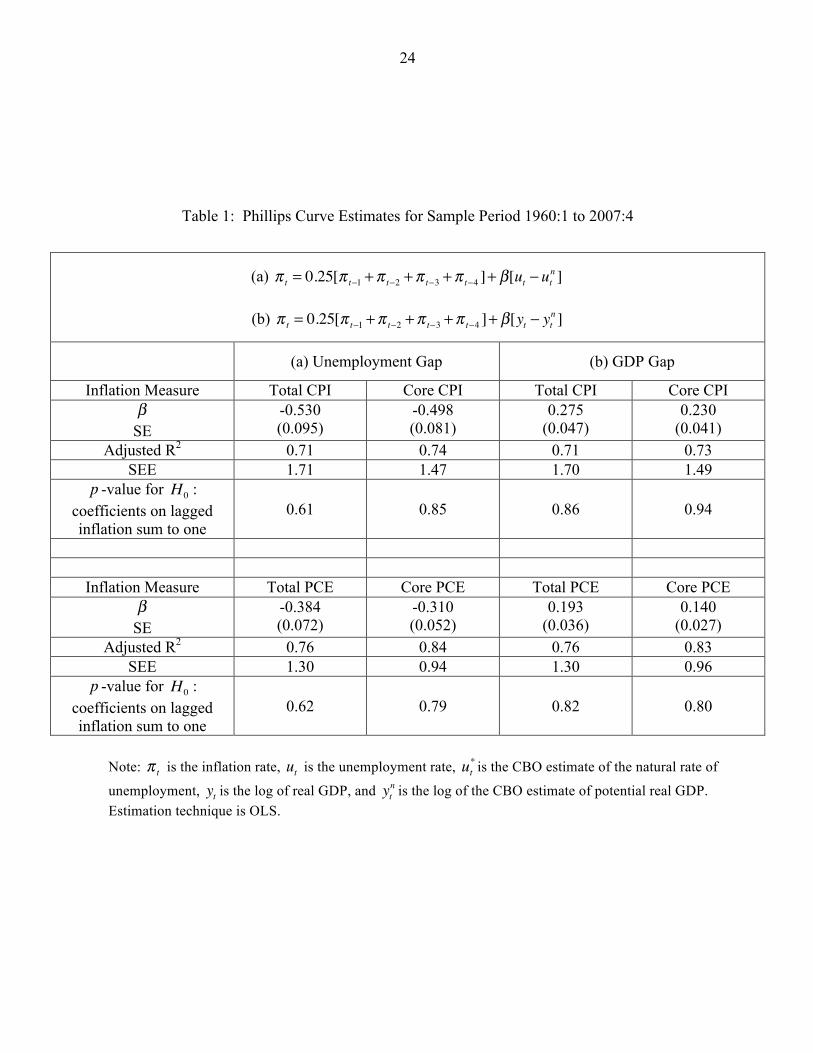
Table 1 presents OLS estimates of equation (3) over the period 1960-2007 using

quarterly data for inflation measured using the consumer price index (CPI) and the approach to estimating Phillips curve models in maintaining that expected inflation depends on lagged values of actual inflation. 8 Recently the CBO has provided a two estimates, one of which accounts for temporary labor market conditions that have elevated the natural rate since 2008. I use this CBO “short-run” natural rate in constructing the unemployment gap. 9 By contrast, the New Keynesian Phillips curve implies that inflation is expected to decline when unemployment is below its natural rate, as Roberts (1995) illustrates. I report results for specifications of the New Keynesian Phillips curve in an Appendix to this paper, showing that, like the accelerationist Phillips curve, it also is unable to explain the recent behavior of inflation. 10 See also Murphy (1986), who discusses a break around 1959 in the process determining inflation expectations as measured by the Livingston expected inflation survey maintained by the Federal Reserve Bank of Philadelphia.

7

personal consumption expenditures price index (PCE). I report estimates for both total

inflation and inflation less food and energy prices (denoted “core”), and for the GDP gap

in addition to the unemployment gap.11 In all cases, the coefficient on the gap variable is

of the correct sign (negative for the unemployment gap and positive for the GDP gap)

and statistically different from zero at high levels of confidence. The restriction that the

coefficients on lagged inflation sum to one cannot be rejected.

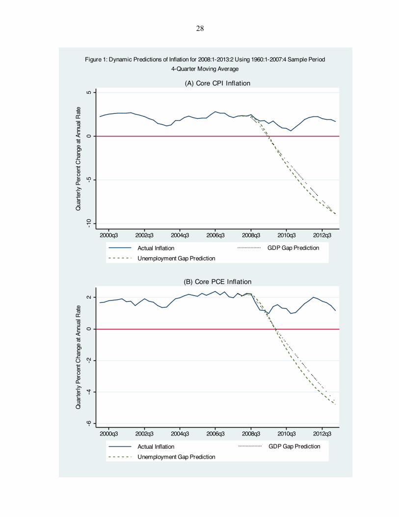
Figure 1 shows predictions from equation (3) when it is estimated over the period

1960-2007 and then simulated through second quarter of 2013. These dynamic

simulations use lagged values of predicted inflation to form the expected inflation

variable and actual values of the gap variable.12 Figure 1 presents results for core

inflation (CPI in panel A and PCE in panel B) with predictions using the two gap series.

The inflation rates shown in these figures are four-quarter moving averages, which help

smooth out fluctuations in the quarterly data. For both inflation series shown in Figure 1,

the model predicts deflation during the last several years regardless of the measure used

for the gap variable. Simulations using total inflation (not shown) likewise predict

deflation.13

11 All estimates in this paper use data available as of December 1, 2013, which include the July 2013 Comprehensive Revision of the National Income Accounts by the Bureau of Economic Analysis. Due to changes in methodology, these estimates increased significantly the level of GDP. The Congressional Budget Office has not yet released a comparable potential GDP series, so I use the most recent estimates of the GDP gap provided in February 2013. 12 Because the goal of this paper is to assess how well the Phillips curve explains the recent behavior of inflation, I use actual values of the “exogenous” gap variable rather than values for the gap variable that might have been forecast at the end of the estimation period in 2007. 13 I do not consider median inflation in this paper but focus instead on explaining the behavior of core inflation as measured by the traditional metrics of the CPI less food and energy and the PCE price index less food and energy. My reason for this is two fold. First, these standard measures of inflation are used to frame monetary policy discussions and so seem most relevant for analysts trying to assess potential policy response to economic conditions.13 Second, the Phillips curve historically has performed quite well in describing the behavior of these traditional core measures, so it seems sensible to explore whether additional modifications to the model, rather than a change in how we measure core inflation, might help explain the recent behavior.

8

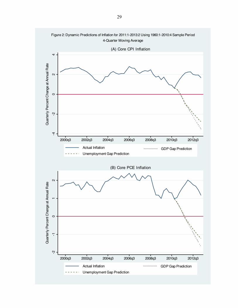
As a check on the robustness of these deflation predictions, I extended the

estimation sample. Figure 2 shows predictions through the second quarter of 2013 when

the estimation sample is 1960 to 2010. Once again, the model predicts deflation. Results

using estimation samples ending in 2008 and 2009 are broadly similar to those shown in

Figures 1 and 2, predicting deflation soon after the estimation period ends—deflation that

has not in fact occurred.

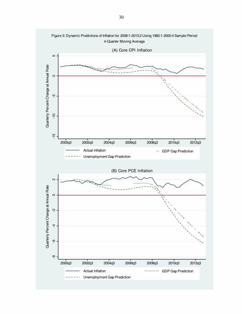
Much policy discussion in the early 2000s centered on concern that the U.S.

economy was flirting with deflation.14 This raises the question of how well the Phillips

curve performed over the years leading up to the Great Recession. Figure 3 presents

predictions when the estimation sample ends in 2000 and the model is simulated

dynamically through second quarter of 2013. As seen in Panel A, the model predicts core

CPI inflation reasonably well through 2007 using the GDP gap, although it under-

predicts starting in 2004 using the unemployment gap. For core PCE inflation shown in

panel B, the model under-predicts starting in 2004 for both measures of the gap. These

results indicate that the inflation may have become less sensitive to demand conditions in

the years prior to the Great Recession.

3. The Time-Varying Response of Inflation to Economic Slack

One possible reason for the failure of standard Phillips curve models to explain

the recent behavior of inflation is that the slope coefficient on the gap term may vary

through time and recently may have become much smaller than the value estimated using

data for the past fifty years. In this section, I present evidence that confirms a decline in

14 See speeches by Federal Reserve Chair Alan Greenspan (2002) and Federal Reserve Governor Ben Bernanke (2002).

9

the slope of the Phillips curve using a rolling regression technique. I also test formally

for a breakpoint in the relationship and find evidence of a shift in the early 1980s and

possibly the early 1990s.

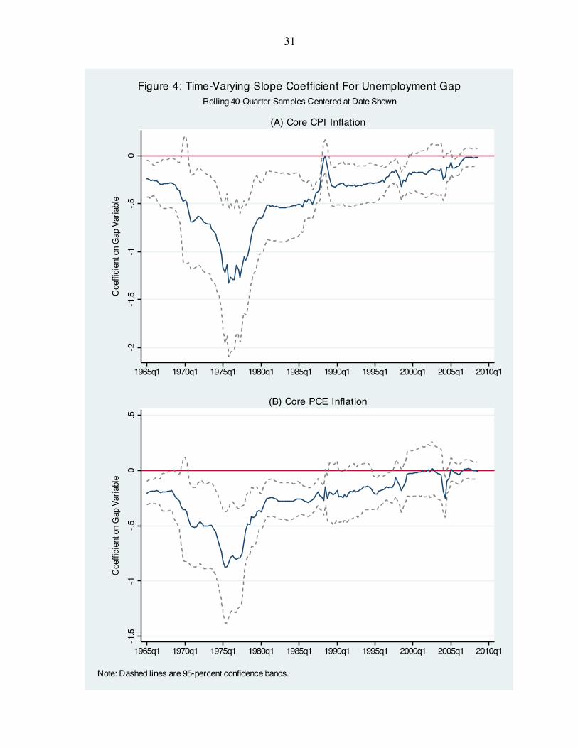
Figure 4 presents estimates of the slope parameter β in equation (3) using rolling

regressions with 10-year (40-quarter) windows for the period 1960-2013. For both CPI

and PCE inflation, the absolute value of the slope parameter is low in the 1960s, rises in

the 1970s, declines in the 1980s, and then gradually trends downward through the 1990s,

falling toward zero in the 2000s.15 This pattern qualitatively matches those estimated

using more sophisticated time-series techniques, such as in Stock and Watson (2010) or

Ball and Mazumder (2011).

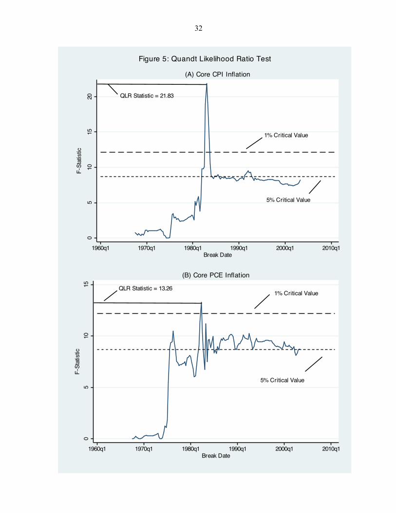
Figure 5 shows results of a Quandt Likelihood Ratio test for an unknown

structural break in the relationship between inflation and the unemployment gap.16 For

both core CPI inflation (panel A) and core PCE inflation (panel B) the maximum occurs

in the early 1980s and is significant at the one-percent level of confidence. Another

smaller peak, significant at the five-percent level, is present in the early 1990s for core

CPI inflation, suggesting a second possible breakpoint, although a formal test for the

period from 1983 onward (not shown) could not reject the hypothesis of no structural

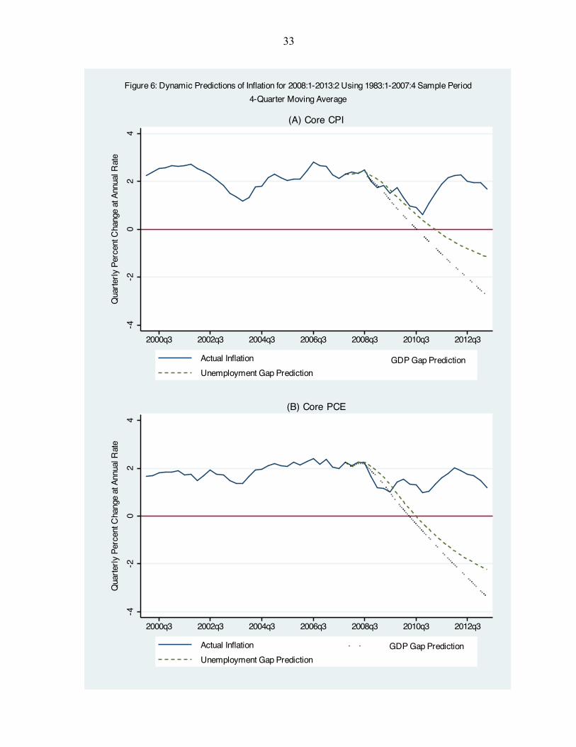
break. Estimates using data from 1983 to 2007, reported in Figure 6, show that the model

continues to underpredict inflation, although by substantially less than when estimated for

the full sample period.

15 Results for the GDP gap are similar. 16 The test involves computing the F-statistic for a Chow test of the null hypothesis of no structural break at each observation over the inner 70 percent of the sample and then choosing the maximum value as the QLR statistic. Confidence levels for the QLR statistic shown in Figure 5 are taken from Table 14.6 in Stock and Watson (2010).

10

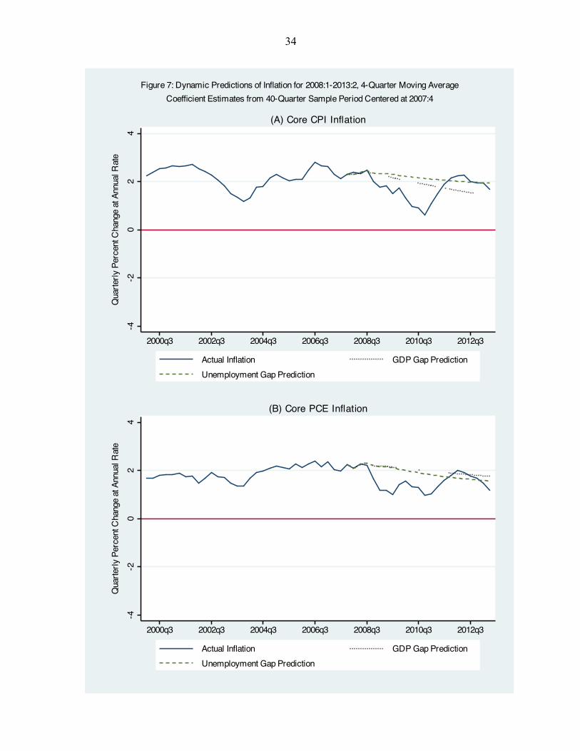
As Figure 4 illustrates, point estimates of the slope coefficient declined in

absolute value during the 2000s, becoming quite small. Figure 7 provides predictions

using coefficient estimates from a 40-quarter window centered at the fourth quarter of

2007 (i.e., a sample period of 2003 through 2012). For this in-sample simulation, the

model no longer predicts deflation, owing to the attenuated response of inflation to the

gap variables. These results suggest that explicitly modeling time-variation of the slope

coefficient may help explain the recent behavior of inflation.

4. Explaining Time Variation in the Phillips Curve’s Slope

This section investigates reasons why the Phillips curve’s slope may vary through

time. I consider implications of price-setting models when prices are costly to adjust and

information is costly to obtain. My analysis is not a formal test of these forward-looking

price-setting models but instead uses these models’ implications to motivate why the

Phillips curve’s slope may vary with the inflation environment and uncertainty about

regional economic conditions.

As shown in Figure 4, the slope coefficient for the Phillips curve declined sharply

in absolute value during the late 1970s and early 1980s, and then gradually trended lower

in the 1990s, falling close to zero in the 2000s. This suggests that controlling explicitly

for economic conditions that influence the magnitude of the slope coefficient should help

improve the predictive performance of the Phillips curve.

In the sticky-price model, firms face fixed costs of adjusting prices and so find it

optimal to hold prices constant for some period of time. The frequency with which firms

adjust depends on uncertainty about market conditions as well as the average level of

11

inflation. When uncertainty about market conditions is low, the probability also is low

that a firm’s fixed price will deviate a lot from its optimal value and so firms will hold

prices fixed for a longer period of time than when uncertainty is high. Similarly, when

the average level of inflation is low, firms will find it optimal to hold prices fixed for a

longer period of time because with low inflation it takes longer for the firm’s fixed price

to deviate from its optimal level. Accordingly, the sticky-price model predicts that the

response of inflation to slack in the economy varies directly with uncertainty about

market conditions and the level of inflation.17

By contrast, the sticky-information model assumes prices are costless to change

but information about market conditions is costly to acquire. Firms set a path for their

prices given current information.18 They update their price path only when the perceived

benefit of acquiring information exceeds its cost. Greater uncertainty about market

conditions, and hence greater uncertainty about whether a firm’s price path is out of line

with competitors, will increase the perceived benefit of acquiring information and lead to

more frequent updating. Thus, the sticky-information model also predicts that the slope

of the Phillips curve will vary over time with changes in uncertainty about a firm’s

market conditions.19 But unlike the sticky-price model, the sticky-information model

predicts that the average level of inflation has no effect on the responsiveness of prices to

aggregate demand. The reason for this is that inflation has no effect on the frequency of

17 See Ball, Mankiw, and Romer (1988) for a discussion of the sticky-price model’s implications for the slope of the Phillips curve. 18 See Mankiw and Reis (2007, 2010) for overviews of price-setting models in which information is imperfect. 19 Reis (2006) shows that greater uncertainty about a firm’s market conditions reduces the time between information updates, thereby increasing the responsiveness of prices and inflation to aggregate demand.

12

information updates because price paths set by firms fully incorporate the average level

of inflation.

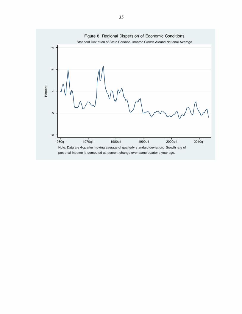
I assume that uncertainty about market conditions can be approximated by

uncertainty about inflation (measured using the standard deviation of inflation) and by

uncertainty about regional economic conditions. As a proxy for uncertainty about

regional economic conditions, I use the standard deviation of growth in state personal

income relative to growth in national personal income. The growth rate is computed as

the percent change over the same quarter a year ago. I calculate the standard deviation

for each quarter using data for all fifty states.

Figure 8 shows this regional dispersion variable, computed as a four-quarter

moving average to smooth out quarterly volatility. The dispersion measure is relatively

low in the 1960s, rises sharply and becomes more volatile in the 1970s, and then declines

and becomes less volatile from the mid-1980s onward. This pattern broadly matches the

estimates of time-variation in the slope coefficient of the Phillips curve shown earlier in

Figure 4.

Figure 9 plots the mean and standard deviation of inflation, computed on a rolling

basis over 40-quarter intervals.20 These measures of the inflation environment are low in

the 1960s, increase in the 1970s, decline in the 1980s through the 1990s, and remain low

in the 2000s. This pattern likewise qualitatively matches the time-variation in the slope

coefficient of the Phillips curve, although both of the inflation series exhibit much less

volatility than the regional dispersion series.

20 The rolling estimates are centered at the midpoint of the 40-quarter windows. I fill out the first and last 20 quarters using the estimates from the first and last 40-quarter windows.

13

To assess whether accounting for the inflation environment and/or regional

dispersion in economic conditions improves the ability of the Phillips curve to explain

recent inflation, I modify equation (3) to allow the slope coefficient to vary over time. In

particular, I estimate variants of the following equation:

(4) π t = 0.25[π t−1 +π t−2 +π t−3 +π t−4 ]+ β0[ut − ut

n ] + β1π t[ut − ut

n ]+ β2σ tπ [ut − ut

n ]+ β3σ ty[ut − ut

n ]

where π t and σ tπ are four-quarter moving averages of the mean and standard deviation of

inflation, and σ ty is the four-quarter moving average of the standard deviation of

quarterly state personal income growth around national personal income growth. The

interaction terms capture variation in the slope coefficient over time.21

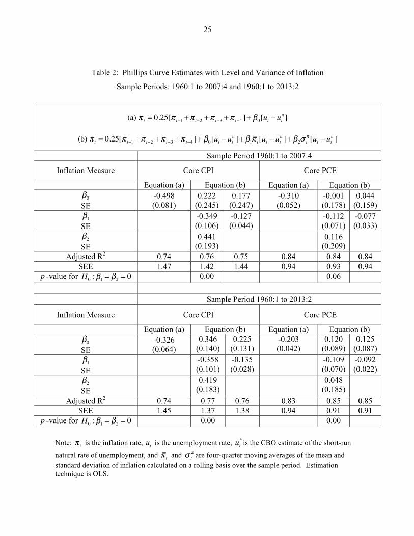
Table 2 reports estimates of two variants of equation (4), first reproducing the

earlier results without interaction terms, denoted (a) in the table, and then providing

estimates including the inflation environment terms, π t and σ tπ , denoted (b). I provide

estimates for the period 1960 to 2007 and for the period 1960 through the second quarter

of 2013.22 The coefficients on the inflation environment terms (β1 and β2 ) are each

statistically significant at the five-percent level for estimates using core CPI inflation,

although the coefficient on the inflation variance term (β2 ) has an incorrect (positive)

21 This specification of the Phillips curve allows the slope coefficient to vary with the inflation environment and uncertainty about regional economic conditions. The equation is not intended to be a representation of the Mankiw and Reis (2002) sticky-information Phillips curve or the sticky-price New Keynesian Phillips curve. I use those frameworks only to motivate in a general sense why the slope coefficient might vary over time. 22 In the interests of brevity, I only show estimates for specifications using the unemployment gap in Tables 2 and 3. Estimates using the GDP gap are qualitatively similar.

14

sign. For core PCE inflation, the coefficients are only jointly, not individually,

significant and the coefficient on the inflation variance term again has an incorrect

(positive) sign. A high degree of collinearity between π t and σ tπ apparently makes the

individual effects hard to distinguish—when the mean of inflation, π t , is entered alone

(second column under variant (b)), its coefficient is always statistically significant and of

the correct sign.23 These results provide only weak support for the sticky-price model’s

implication that the average level of inflation influences the slope of the Phillips curve,

while the positive coefficient on the variance term is at odds with implications of both the

sticky price and sticky information approaches to price setting.

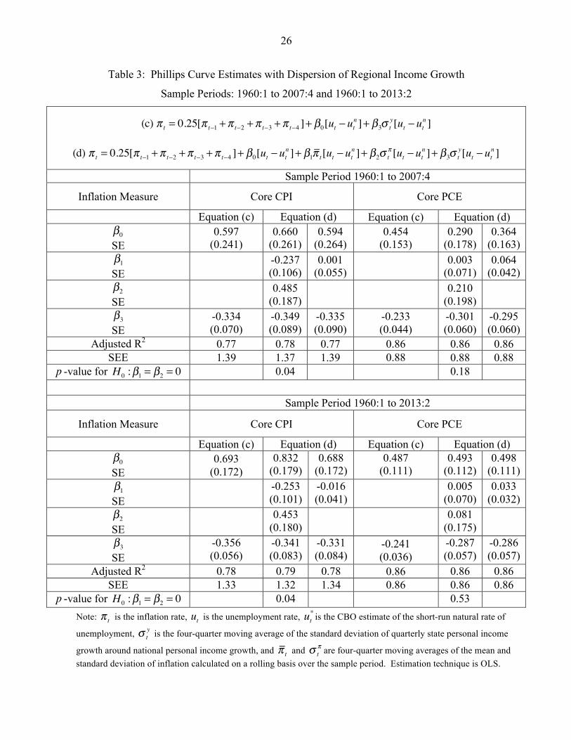
Table 3 reports estimates for two variants of equation (4) that include the regional

dispersion term, σ ty . I present results for the dispersion term alone, denoted (c) in the

table, and in combination with the inflation environment terms, denoted (d). As before, I

provide estimates for the period 1960 to 2007 and for the period 1960 through the second

quarter of 2013. The coefficient on the regional dispersion term (β3 ) is statistically

significant at the one-percent level in all specifications, and has the correct (negative)

sign. When I include both the dispersion term and the inflation environment terms (first

column under variant (d)), the coefficients on the latter (β1 and β2 ) are statistically

significant at the five-percent level for core CPI inflation, although the coefficient on the

inflation variance term (β2 ) again has an incorrect (positive) sign. For estimates using

core PCE inflation, the coefficients on the inflation terms are not statistically significant,

either individually or jointly. Interestingly, when the mean of inflation term, π t , alone is

23 When the variance of inflation variance term is entered alone (not shown), its coefficient is not significant.

15

included with the regional dispersion term (second column under variant (d)), its

coefficient is never statistically significant, while the coefficient on the dispersion term

always has the correct (negative) sign, is statistically significant, and stable across

specifications.24

The results in Tables 2 and 3 indicate that time variation in the slope of the

Phillips curve is more closely related to regional dispersion of income growth than to the

inflation environment. I interpret this as suggesting that uncertainty about regional

economic conditions, as measured by the regional dispersion of income growth, helps

explain time variation in the slope of the Phillips curve. As discussed earlier, the average

level of inflation should affect the slope of the Phillips curve in the sticky-price model

but not the sticky-information model. Because the interaction term for the mean of

inflation loses significance when combined with the regional dispersion term, the results

seem more supportive of the sticky-information approach, although uncertainty about

regional economic conditions certainly should also matter for firms setting prices under

the sticky-price approach.

Given that these interaction terms find some statistical support, I repeat the earlier

exercise of predicting recent inflation but now use variants (c) and (d) reported in Table 3

in which the slope varies continuously. As before, I estimate the model over the period

1960 to 2007 and then dynamically forecast inflation through the second quarter of 2013.

I also estimate the model over the period 1960 to 2000 and forecast inflation through the

second quarter of 2013 as a check on whether either variant can explain inflation during

the early 2000s.

24 When the inflation variance term alone is included with the regional dispersion term (not shown), its coefficient is never statistically significant, while the coefficient on the regional dispersion term is negative and significant.

16

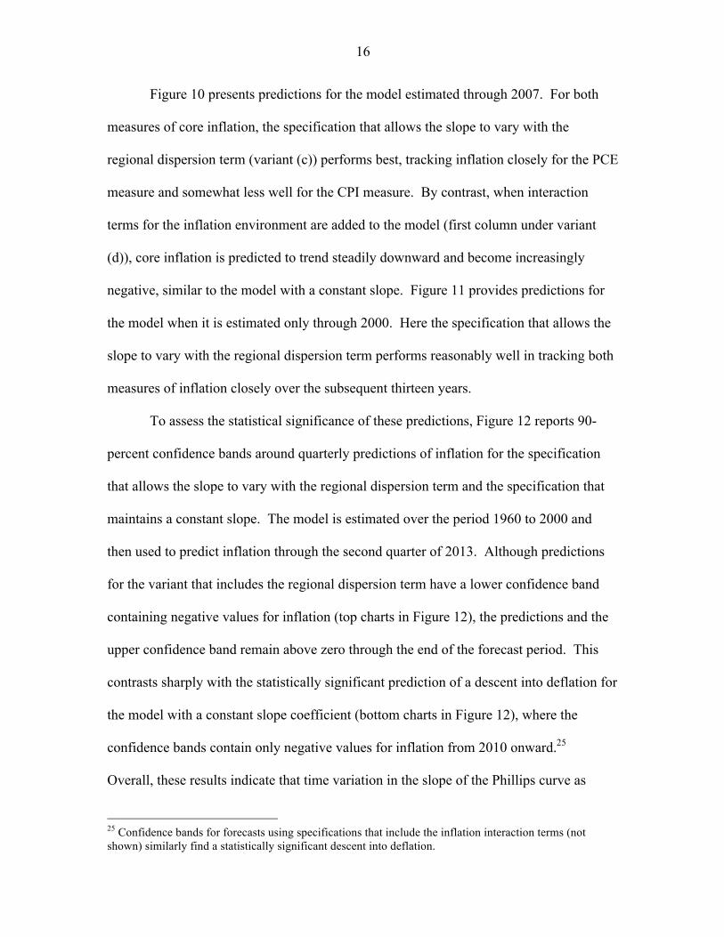
Figure 10 presents predictions for the model estimated through 2007. For both

measures of core inflation, the specification that allows the slope to vary with the

regional dispersion term (variant (c)) performs best, tracking inflation closely for the PCE

measure and somewhat less well for the CPI measure. By contrast, when interaction

terms for the inflation environment are added to the model (first column under variant

(d)), core inflation is predicted to trend steadily downward and become increasingly

negative, similar to the model with a constant slope. Figure 11 provides predictions for

the model when it is estimated only through 2000. Here the specification that allows the

slope to vary with the regional dispersion term performs reasonably well in tracking both

measures of inflation closely over the subsequent thirteen years.

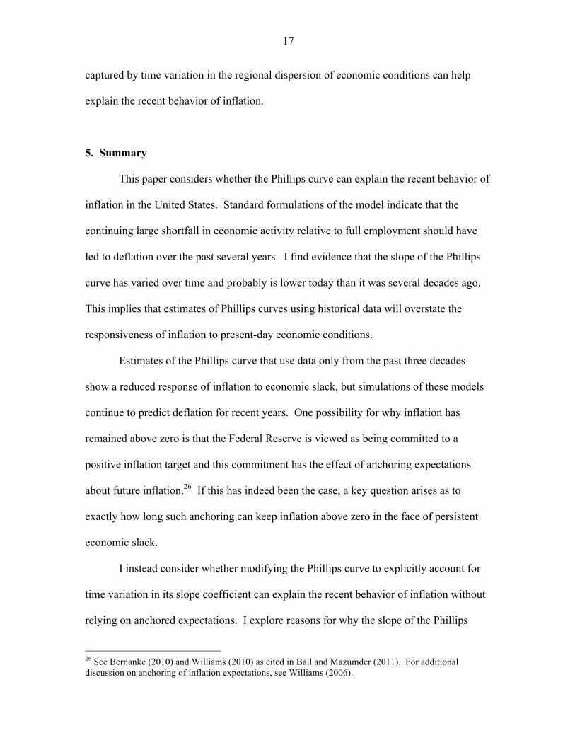
To assess the statistical significance of these predictions, Figure 12 reports 90-

percent confidence bands around quarterly predictions of inflation for the specification

that allows the slope to vary with the regional dispersion term and the specification that

maintains a constant slope. The model is estimated over the period 1960 to 2000 and

then used to predict inflation through the second quarter of 2013. Although predictions

for the variant that includes the regional dispersion term have a lower confidence band

containing negative values for inflation (top charts in Figure 12), the predictions and the

upper confidence band remain above zero through the end of the forecast period. This

contrasts sharply with the statistically significant prediction of a descent into deflation for

the model with a constant slope coefficient (bottom charts in Figure 12), where the

confidence bands contain only negative values for inflation from 2010 onward.25

Overall, these results indicate that time variation in the slope of the Phillips curve as

25 Confidence bands for forecasts using specifications that include the inflation interaction terms (not shown) similarly find a statistically significant descent into deflation.

17

captured by time variation in the regional dispersion of economic conditions can help

explain the recent behavior of inflation.

5. Summary

This paper considers whether the Phillips curve can explain the recent behavior of

inflation in the United States. Standard formulations of the model indicate that the

continuing large shortfall in economic activity relative to full employment should have

led to deflation over the past several years. I find evidence that the slope of the Phillips

curve has varied over time and probably is lower today than it was several decades ago.

This implies that estimates of Phillips curves using historical data will overstate the

responsiveness of inflation to present-day economic conditions.

Estimates of the Phillips curve that use data only from the past three decades

show a reduced response of inflation to economic slack, but simulations of these models

continue to predict deflation for recent years. One possibility for why inflation has

remained above zero is that the Federal Reserve is viewed as being committed to a

positive inflation target and this commitment has the effect of anchoring expectations

about future inflation.26 If this has indeed been the case, a key question arises as to

exactly how long such anchoring can keep inflation above zero in the face of persistent

economic slack.

I instead consider whether modifying the Phillips curve to explicitly account for

time variation in its slope coefficient can explain the recent behavior of inflation without

relying on anchored expectations. I explore reasons for why the slope of the Phillips

26 See Bernanke (2010) and Williams (2010) as cited in Ball and Mazumder (2011). For additional discussion on anchoring of inflation expectations, see Williams (2006).

18

curve might vary over time, focusing on implications of the sticky-price and sticky-

information approaches to price adjustment. These implications suggest that the inflation

environment and the extent of uncertainty about regional economic conditions should

influence the slope of the Phillips curve. I modify the Phillips curve by introducing

proxies to account for these effects and find that the dispersion of regional economic

activity is helpful for explaining the recent path of inflation.

Future research should investigate formal implications of the sticky-price and

sticky-information models for time-variation in the slope of the Phillips curve. In

particular, state-dependent versions of the sticky-price and sticky-information models

could provide frameworks to directly test the intuitive notion used in this paper that the

timing of price adjustment and information acquisition is endogenous. Other proxies for

uncertainty about regional economic conditions also could be explored and tested in the

Phillips curve framework.

19

Appendix: The New Keynesian Phillips Curve As derived by Roberts (1995), a basic version of the sticky-price New Keynesian

Phillips curve expresses current inflation as a function of the rate of inflation expected for

next period and the gap between unemployment and its natural rate (or alternatively, the

output gap):

(A.1) π t = Etπ t+1 + β ut − utn⎡⎣ ⎤⎦ + ε t

where β < 0 (β > 0 for the output gap), and ε is an error term. The gap variable is

intended to capture movements in marginal cost that influence price setting behavior by

firms.

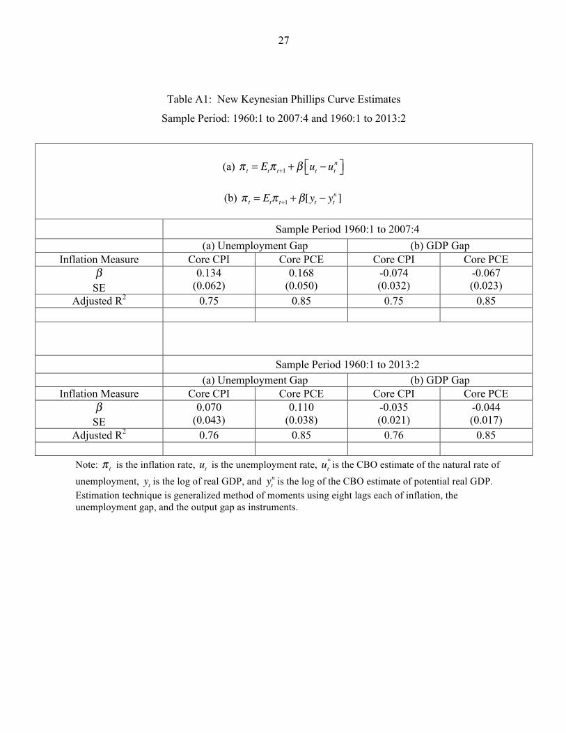
Table A1 provides estimates of equation (A.1) using the generalized method of

moments applied to the following orthogonality condition:

(A.2) Et{(π t − β ut − utn⎡⎣ ⎤⎦ −π t+1)z't } = 0

where the z't is a vector of instruments containing eight lags each of inflation, the

unemployment gap, and the output gap. I employ the same gap variables used in Table 1

of the text for comparability with those results and because standard measures of

marginal cost based on labor share have been shown by Mazumder (2010, 2011) to be

poor proxies for marginal cost faced by firms.

As seen in Table A1, the coefficient on the gap variables is statistically significant

at the five-percent level for both core PCE and core CPI inflation over the period 1960 to

20

2007, but of the incorrect sign rejecting the specification of equation (A.1). For the

period 1960 into 2013, the estimate for core PCE inflation is statistically significant while

those for core CPI inflation is only weakly significant (ten-percent level), but again the

coefficient has the wrong sign. These results are consistent with Mankiw (2001), Ball

and Mazumder (2011), and other authors who demonstrate the poor performance of this

specification of the Phillips curve. The results indicate that slack in the economy is

associated with an expected decline in inflation, not the increase implied by the New

Keynesian Phillips curve.

Figure 1A shows the four-quarter moving average of the predictions from

equation (A.1) when it is estimated over the period 1960 to 2007 and then simulated

through second quarter of 2013. The model does poorly and predicts a sharp decent into

deflation, similar to results using the traditional backward-looking Phillips curve

illustrated in Figure 1 of the text.

21

References

Ball, L., N. Mankiw, and D. Romer (1988): “The New Keynsesian Economics and the Output-Inflation Trade-off,” Brookings Papers on Economic Activity, 19, 1–82. Ball, L. and S. Mazumder (2011): “Inflation Dynamics and the Great Recession,” Brookings Papers on Economic Activity, Spring 2011, 337–381. Barsky, R. (1987): “The Fisher Hypothesis and the Forecastability and Persistence of Inflation,” Journal of Monetary Economics, 19, 3–24. Bernanke, B. (2002): “Deflation: Making Sure “It” Doesn’t Happen Here,” Remarks before the National Economists Club, Washington, DC, November 21, 2002. Bernanke, B. (2008): “Outstanding Issues in the Analysis of Inflation,” in Understanding Inflation and the Implications for Monetary Policy, ed. by J. Fuhrer, Y. Kodrzycki, J. Little and G. Olivei, MIT Press, 447-456. Bernanke, B. (2010): “The Economic Outlook and Monetary Policy,” Speech at the Federal Reserve Bank of Kansas City Economic Symposium, Jackson Hole, Wyoming. Calvo, G. (1983): “Staggered Prices in a Utility Maximizing Framework,” Journal of Monetary Economics, 12, 383–398. Congressional Budget Office (2013): “The Budget and Economic Outlook: Fiscal Years 2013 to 2023,” February 2013, Washington, DC. Friedman, M. (1968): “The Role of Monetary Policy,” American Economic Review, 58, 1–17. Fuhrer, J. (1995): “The Phillips Curve is Alive and Well,” New England Economic Review, March/April, 41-56. Gordon, R. (1982): “Inflation, Flexible Exchange Rates, and the Natural Rate of Unemployment,” in Workers, Jobs, and Inflation, ed. by M. Baily, The Brookings Institution, 89–158. Gordon, R. (1990): “U.S. Inflation, Labor’s Share, and the Natural Rate of Unemployment,” in Economics of Wage Determination, ed. by H. Koenig, Berlin: Springer-Verlag.

22

Greenspan, A. (2002): “Issues for Monetary Policy,” Remarks before the Economic Club of New York, New York City, December 19, 2002. Lucas, R. (1973): “Some International Evidence on Output-Inflation Tradeoffs,” American Economic Review, 63, 326–34. Mankiw, N. (2001): “The Inexorable and Mysterious Tradeoff Between Inflation and Unemployment,” Economic Journal, 111, C45-C61. Mankiw, N. and R. Reis (2002): “Sticky Information Versus Sticky Price: A Proposal to Replace the New Keynesian Phillips Curve,” Quarterly Journal of Economics, 117, 1295– 1328. Mankiw, N. and R. Reis (2007): “Sticky Information in General Equilibrium,” Journal of the European Economic Association, 2, 603-13. Mankiw, N. and R. Reis (2010): “Chapter 5 - Imperfect Information and Aggregate Supply,” in Handbook of Monetary Economics, ed. by B. Friedman and M. Woodford, Elsevier, Volume 3, 183-229. Mankiw, N., R. Reis, and J. Wolfers (2003): “Disagreement about Inflation Expectations,” NBER Working Paper #9796, June 2003. Mazumder, S. (2010): “The New Keynesian Phillips Curve and the Cyclicality of Marginal Cost,” Journal of Macroeconomics, 32, 747-65. Mazumder, S. (2011): “Cost-based Phillips Curve Forecasts of Inflation,” Journal of Macroeconomics, 33, 553-67. Murphy, R. (1986): “The Expectations Theory of the Term Structure: Evidence from Inflation Forecasts,” Journal of Macroeconomics, 8, 423-34. Murphy, R. (1999): “Accounting for the Recent Decline in the NAIRU,” Business Economics, Volume 34. Murphy, R. (2000): “What’s Behind the Decline in the NAIRU?” in The Economic Outlook For 2000, ed. by S. Hymans, University of Michigan, January 2000. Murphy, R. (2014): “Explaining Inflation in the Aftermath of the Great Recession,” Journal of Macroeconomics, 40, 228-44.

23

Reinhart, C. and K. Rogoff (2009): This Time Is Different: Eight Centuries of Financial Folly, Princeton University Press. Reis, R. (2006): “Inattentive Producers,” Review of Economic Studies, 73, 793-821. Roberts, J. (1995): “New Keynesian Economics and the Phillips Curve,” Journal of Money, Credit, and Banking, 27, 975–984. Staiger, D., J. Stock, and M. Watson (1997): “How Precise Are Estimates of the Natural Rate of Unemployment?” in Reducing Inflation: Motivation and Strategy, NBER, 195–246. Stock, J. and M. Watson (2008): “Phillips Curve Inflation Forecasts,” NBER Working Paper, 14322. Stock, J. and M. Watson (2010): “Modeling Inflation After the Crisis,” NBER Working Paper, 16488. Stock, J. and M. Watson (2010): Introduction to Econometrics, Prentice Hall. Williams, J. (2006): “Inflation Persistence in an Era of Well-anchored Inflation Expectations,” FRBSF Economic Letter, 2006-27. Williams, J. (2010): “Sailing into Headwinds: The Uncertain Outlook for the U.S. Economy,” Presentation to Joint Meeting of the San Francisco and Salt Lake City Branch Boards of Directors, Salt Lake City, UT.

24

Table 1: Phillips Curve Estimates for Sample Period 1960:1 to 2007:4

(a) π t = 0.25[π t−1 +π t−2 +π t−3 +π t−4 ]+ β[ut − utn ]

(b) π t = 0.25[π t−1 +π t−2 +π t−3 +π t−4 ]+ β[yt − yt

n ]

(a) Unemployment Gap (b) GDP Gap

Inflation Measure Total CPI Core CPI Total CPI Core CPI β

SE -0.530 (0.095)

-0.498 (0.081)

0.275 (0.047)

0.230 (0.041)

Adjusted R2 0.71 0.74 0.71 0.73 SEE 1.71 1.47 1.70 1.49

p -value for H0 : coefficients on lagged inflation sum to one

0.61 0.85 0.86 0.94

Inflation Measure Total PCE Core PCE Total PCE Core PCE β

SE -0.384 (0.072)

-0.310 (0.052)

0.193 (0.036)

0.140 (0.027)

Adjusted R2 0.76 0.84 0.76 0.83 SEE 1.30 0.94 1.30 0.96

p -value for H0 : coefficients on lagged inflation sum to one

0.62 0.79 0.82 0.80

Note: π t is the inflation rate, ut is the unemployment rate, ut

* is the CBO estimate of the natural rate of

unemployment, yt is the log of real GDP, and ytn is the log of the CBO estimate of potential real GDP.

Estimation technique is OLS.

25

Table 2: Phillips Curve Estimates with Level and Variance of Inflation

Sample Periods: 1960:1 to 2007:4 and 1960:1 to 2013:2

(a) π t = 0.25[π t−1 +π t−2 +π t−3 +π t−4 ]+ β0[ut − utn ]

(b) π t = 0.25[π t−1 +π t−2 +π t−3 +π t−4 ]+ β0[ut − ut

n ]+ β1π t[ut − utn ]+ β2σ t

π [ut − utn ]

Sample Period 1960:1 to 2007:4

Inflation Measure Core CPI Core PCE

Equation (a) Equation (b) Equation (a) Equation (b) β0 SE

-0.498 (0.081)

0.222 (0.245)

0.177 (0.247)

-0.310 (0.052)

-0.001 (0.178)

0.044 (0.159)

β1 SE

-0.349 (0.106)

-0.127 (0.044) -0.112

(0.071) -0.077 (0.033)

β2 SE

0.441 (0.193) 0.116

(0.209)

Adjusted R2 0.74 0.76 0.75 0.84 0.84 0.84 SEE 1.47 1.42 1.44 0.94 0.93 0.94

p -value for H0 :β1 = β2 = 0 0.00 0.06 Sample Period 1960:1 to 2013:2


Equation (a) Equation (b) Equation (a) Equation (b) β0 SE

-0.326 (0.064)

0.346 (0.140)

0.225 (0.131)

-0.203 (0.042)

0.120 (0.089)

0.125 (0.087)

β1 SE

-0.358 (0.101)

-0.135 (0.028)

-0.109 (0.070)

-0.092 (0.022)

β2 SE

0.419 (0.183)

0.048 (0.185)

Adjusted R2 0.74 0.77 0.76 0.83 0.85 0.85 SEE 1.45 1.37 1.38 0.94 0.91 0.91

p -value for H0 :β1 = β2 = 0 0.00 0.00

Note: π t is the inflation rate, ut is the unemployment rate, ut* is the CBO estimate of the short-run

natural rate of unemployment, and π t and σ tπ are four-quarter moving averages of the mean and

standard deviation of inflation calculated on a rolling basis over the sample period. Estimation technique is OLS.

26

Table 3: Phillips Curve Estimates with Dispersion of Regional Income Growth

Sample Periods: 1960:1 to 2007:4 and 1960:1 to 2013:2

(c) π t = 0.25[π t−1 +π t−2 +π t−3 +π t−4 ]+ β0[ut − utn ]+ β3σ t

y[ut − utn ]

(d) π t = 0.25[π t−1 +π t−2 +π t−3 +π t−4 ]+ β0[ut − ut

n ]+ β1π t[ut − utn ]+ β2σ t

π [ut − utn ]+ β3σ t

y[ut − utn ]

Sample Period 1960:1 to 2007:4


Equation (c) Equation (d) Equation (c) Equation (d) β0 SE

0.597 (0.241)

0.660 (0.261)

0.594 (0.264)

0.454 (0.153)

0.290 (0.178)

0.364 (0.163)

β1 SE

-0.237 (0.106)

0.001 (0.055) 0.003

(0.071) 0.064

(0.042) β2 SE

0.485 (0.187) 0.210

(0.198)

β3 SE

-0.334 (0.070)

-0.349 (0.089)

-0.335 (0.090)

-0.233 (0.044)

-0.301 (0.060)

-0.295 (0.060)

Adjusted R2 0.77 0.78 0.77 0.86 0.86 0.86 SEE 1.39 1.37 1.39 0.88 0.88 0.88

p -value for H0 :β1 = β2 = 0 0.04 0.18 Sample Period 1960:1 to 2013:2


Equation (c) Equation (d) Equation (c) Equation (d) β0 SE

0.693 (0.172)

0.832 (0.179)

0.688 (0.172)

0.487 (0.111)

0.493 (0.112)

0.498 (0.111)

β1 SE

-0.253 (0.101)

-0.016 (0.041)

0.005 (0.070)

0.033 (0.032)

β2 SE

0.453 (0.180)

0.081 (0.175)

β3 SE

-0.356 (0.056)

-0.341 (0.083)

-0.331 (0.084)

-0.241 (0.036)

-0.287 (0.057)

-0.286 (0.057)

Adjusted R2 0.78 0.79 0.78 0.86 0.86 0.86 SEE 1.33 1.32 1.34 0.86 0.86 0.86

p -value for H0 :β1 = β2 = 0 0.04 0.53 Note: π t is the inflation rate, ut is the unemployment rate, ut

* is the CBO estimate of the short-run natural rate of

unemployment, σ ty is the four-quarter moving average of the standard deviation of quarterly state personal income

growth around national personal income growth, and π t and σ tπ are four-quarter moving averages of the mean and

standard deviation of inflation calculated on a rolling basis over the sample period. Estimation technique is OLS.

27

Table A1: New Keynesian Phillips Curve Estimates

Sample Period: 1960:1 to 2007:4 and 1960:1 to 2013:2

(a) π t = Etπ t+1 + β ut − utn⎡⎣ ⎤⎦

(b) π t = Etπ t+1 + β[yt − yt

n ]

Sample Period 1960:1 to 2007:4 (a) Unemployment Gap (b) GDP Gap

Inflation Measure Core CPI Core PCE Core CPI Core PCE β

SE 0.134

(0.062) 0.168

(0.050) -0.074 (0.032)

-0.067 (0.023)

Adjusted R2 0.75 0.85 0.75 0.85

Sample Period 1960:1 to 2013:2 (a) Unemployment Gap (b) GDP Gap

Inflation Measure Core CPI Core PCE Core CPI Core PCE β

SE 0.070

(0.043) 0.110

(0.038) -0.035 (0.021)

-0.044 (0.017)

Adjusted R2 0.76 0.85 0.76 0.85

Note: π t is the inflation rate, ut is the unemployment rate, ut* is the CBO estimate of the natural rate of

unemployment, yt is the log of real GDP, and ytn is the log of the CBO estimate of potential real GDP.

Estimation technique is generalized method of moments using eight lags each of inflation, the unemployment gap, and the output gap as instruments.

28

-10

-50

5Q

uarte

rly P

erce

nt C

hang

e at

Ann

ual R

ate

2000q3 2002q3 2004q3 2006q3 2008q3 2010q3 2012q3

Actual InflationUnemployment Gap Prediction

GDP Gap Prediction

(A) Core CPI Inflation-6

-4-2

02

Qua

rterly

Per

cent

Cha

nge

at A

nnua

l Rat

e

2000q3 2002q3 2004q3 2006q3 2008q3 2010q3 2012q3


GDP Gap Prediction

(B) Core PCE Inflation

4-Quarter Moving AverageFigure 1: Dynamic Predictions of Inflation for 2008:1-2013:2 Using 1960:1-2007:4 Sample Period

29

-4-2

02

4Q

uarte

rly P

erce

nt C

hang

e at

Ann

ual R

ate

2000q3 2002q3 2004q3 2006q3 2008q3 2010q3 2012q3


GDP Gap Prediction


-10

12

Qua

rterly

Per

cent

Cha

nge

at A

nnua

l Rat

e

2000q3 2002q3 2004q3 2006q3 2008q3 2010q3 2012q3


GDP Gap Prediction



30

-15

-10

-50

5Q

uarte

rly P

erce

nt C

hang

e at

Ann

ual R

ate

2000q3 2002q3 2004q3 2006q3 2008q3 2010q3 2012q3


GDP Gap Prediction


-6-4

-20

2Q

uarte

rly P

erce

nt C

hang

e at

Ann

ual R

ate

2000q3 2002q3 2004q3 2006q3 2008q3 2010q3 2012q3


GDP Gap Prediction



31

-2-1

.5-1

-.50

Coe

ffici

ent o

n G

ap V

aria

ble

1965q1 1970q1 1975q1 1980q1 1985q1 1990q1 1995q1 2000q1 2005q1 2010q1


.5-1

-.50

.5C

oeffi

cien

t on

Gap

Var

iabl

e

1965q1 1970q1 1975q1 1980q1 1985q1 1990q1 1995q1 2000q1 2005q1 2010q1


Note: Dashed lines are 95-percent confidence bands.

Rolling 40-Quarter Samples Centered at Date ShownFigure 4: Time-Varying Slope Coefficient For Unemployment Gap

32

1% Critical Value

5% Critical Value

QLR Statistic = 21.830

510

1520

F-St

atis

tic

1960q1 1970q1 1980q1 1990q1 2000q1 2010q1Break Date

(A) Core CPI Inflation

1% Critical Value

5% Critical Value

QLR Statistic = 13.26

05

1015

F-St

atis

tic

1960q1 1970q1 1980q1 1990q1 2000q1 2010q1Break Date


Figure 5: Quandt Likelihood Ratio Test

33

-4-2

02

4Q

uarte

rly P

erce

nt C

hang

e at

Ann

ual R

ate

2000q3 2002q3 2004q3 2006q3 2008q3 2010q3 2012q3


GDP Gap Prediction

(A) Core CPI-4

-20

24

Qua

rterly

Per

cent

Cha

nge

at A

nnua

l Rat

e

2000q3 2002q3 2004q3 2006q3 2008q3 2010q3 2012q3


GDP Gap Prediction

(B) Core PCE


34

-4-2

02

4Q

uarte

rly P

erce

nt C

hang

e at

Ann

ual R

ate

2000q3 2002q3 2004q3 2006q3 2008q3 2010q3 2012q3

Actual Inflation GDP Gap PredictionUnemployment Gap Prediction


-20

24

Qua

rterly

Per

cent

Cha

nge

at A

nnua

l Rat

e

2000q3 2002q3 2004q3 2006q3 2008q3 2010q3 2012q3

Actual Inflation GDP Gap PredictionUnemployment Gap Prediction


Coefficient Estimates from 40-Quarter Sample Period Centered at 2007:4Figure 7: Dynamic Predictions of Inflation for 2008:1-2013:2, 4-Quarter Moving Average

35

02

46

8

Perc

ent

1960q1 1970q1 1980q1 1990q1 2000q1 2010q1

Note: Data are 4-quarter moving average of quarterly standard deviation. Growth rate ofpersonal income is computed as percent change over same quarter a year ago.

Standard Deviation of State Personal Income Growth Around National AverageFigure 8: Regional Dispersion of Economic Conditions

36

02

46

8Pe

rcen

t

1960q1 1970q1 1980q1 1990q1 2000q1 2010q1

Mean of Inflation Standard Deviation of Inflation

(A) Core CPI Inflation0

24

68

Perc

ent

1960q1 1970q1 1980q1 1990q1 2000q1 2010q1

Mean of Inflation Standard Deviation of Inflation


Note: Data are 4-quarter moving average of the respective series.

Rolling 40-Quarter Samples Centered at Date ShownFigure 9: Measures of the Inflation Environment

37

-10

-50

5Q

uarte

rly P

erce

nt C

hang

e at

Ann

ual R

ate

2000q3 2002q3 2004q3 2006q3 2008q3 2010q3 2012q3

Actual Inflation Constant SlopeRegional Dispersion Term Only Inflation and Regional Dispersion Terms


-20

2Q

uarte

rly P

erce

nt C

hang

e at

Ann

ual R

ate

2000q3 2002q3 2004q3 2006q3 2008q3 2010q3 2012q3



1960:1-2007:4 Sample Period, 4-Quarter Moving AverageFigure 10: Dynamic Predictions of Inflation for Models with Time Varying Slope

38

-10

-50

5Q

uarte

rly P

erce

nt C

hang

e at

Ann

ual R

ate

2000q3 2002q3 2004q3 2006q3 2008q3 2010q3 2012q3



-4-2

02

Qua

rterly

Per

cent

Cha

nge

at A

nnua

l Rat

e

2000q3 2002q3 2004q3 2006q3 2008q3 2010q3 2012q3



1960:1-2000:4 Sample Period, 4-Quarter Moving AverageFigure 11: Dynamic Predictions of Inflation for Models with Time Varying Slope

39

-15

-10

-50

5

Perc

ent C

hang

e

2000q3 2003q3 2006q3 2009q3 2012q3

Slope Varies With Regional Dispersion TermCore CPI Inflation

-15

-10

-50

5

Perc

ent C

hang

e

2000q3 2003q3 2006q3 2009q3 2012q3

Slope Varies With Regional Dispersion TermCore PCE Inflation

-15

-10

-50

5

Perc

ent C

hang

e

2000q3 2003q3 2006q3 2009q3 2012q3

Constant SlopeCore CPI Inflation

-15

-10

-50

5

Perc

ent C

hang

e

2000q3 2003q3 2006q3 2009q3 2012q3

Constant SlopeCore PCE Inflation

Note: Dotted lines are 90-percent confidence bands around prediction.

Figure 12: Dynamic Predictions of Quarterly Inflation Using 1960:1-2000:4 Sample Period

40

-6-4

-20

24

Qua

rterly

Per

cent

Cha

nge

at A

nnua

l Rat

e

2000q3 2002q3 2004q3 2006q3 2008q3 2010q3 2012q3


GDP Gap Prediction


-4-2

02

Qua

rterly

Per

cent

Cha

nge

at A

nnua

l Rat

e

2000q3 2002q3 2004q3 2006q3 2008q3 2010q3 2012q3


GDP Gap Prediction


1960:1-2007:4 Sample Period, 4-Quarter Moving AverageFigure A1: Dynamic Predictions of Inflation for 2008:1-2013:2 Using New Keynesian Specification

why has inflation been so unresponsive to economic conditions in … pap… · · 2018-03-27why...

Documents