wickham - jss11 - plyr

7/30/2019 Wickham - JSS11 - Plyr

http://slidepdf.com/reader/full/wickham-jss11-plyr 1/29

JSS Journal of Statistical Software April 2011, Volume 40, Issue 1. http://www.jstatsoft.org/

The Split-Apply-Combine Strategy for Data

Analysis

Hadley WickhamRice University

Abstract

Many data analysis problems involve the application of a split-apply-combine strategy,where you break up a big problem into manageable pieces, operate on each piece inde-pendently and then put all the pieces back together. This insight gives rise to a new R

package that allows you to smoothly apply this strategy, without having to worry aboutthe type of structure in which your data is stored.

The paper includes two case studies showing how these insights make it easier to work

with batting records for veteran baseball players and a large 3d array of spatio-temporalozone measurements.

Keywords : R, apply, split, data analysis.

1. Introduction

What do we do when we analyze data? What are common actions and what are commonmistakes? Given the importance of this activity in statistics, there is remarkably little research

on how data analysis happens. This paper attempts to remedy a very small part of that lack bydescribing one common data analysis pattern: Split-apply-combine. You see the split-apply-combine strategy whenever you break up a big problem into manageable pieces, operate oneach piece independently and then put all the pieces back together. This crops up in all stagesof an analysis:

During data preparation, when performing group-wise ranking, standardization, or nor-malization, or in general when creating new variables that are most easily calculated ona per-group basis.

When creating summaries for display or analysis, for example, when calculating marginal

means, or conditioning a table of counts by dividing out group sums.

http://www.jstatsoft.org/




2 The Split-Apply-Combine Strategy for Data Analysis

During modeling, when fitting separate models to each panel of panel data. Thesemodels may be interesting in their own right, or used to inform the construction of a

more sophisticated hierarchical model.

The split-apply-combine strategy is similar to the map-reduce strategy for processing largedata, recently popularized by Google. In map-reduce, the map step corresponds to splitand apply, and reduce corresponds to combine, although the types of reductions are muchricher than those performed for data analysis. Map-reduce is designed for a highly parallelenvironment, where work is done by hundreds or thousands of independent computers, andfor a wider range of data processing needs than just data analysis.

Just recognizing the split-apply-combine strategy when it occurs is useful, because it allowsyou to see the similarly between problems that previously might have appeared unconnected.This helps suggest appropriate tools and frees up mental effort for the aspects of the problem

that are truly unique. This strategy can be used with many existing tools: APL’s arrayoperators (Friendly and Fox 1994), Excel’s pivot tables, the SQL group by operator, and theby argument to many SAS procedures. However, the strategy is even more useful when usedwith software specifically developed to support it; matching the conceptual and computationaltools reduces cognitive impedance. This paper describes one implementation of the strategyin R (R Development Core Team 2010), the plyr package.

In general, plyr provides a replacement for loops for a large set of practical problems, andabstracts away from the details of the underlying data structure. An alternative to loops isnot required because loops are slow (in most cases the loop overhead is small compared to thetime required to perform the operation), but because they do not clearly express intent, asimportant details are mixed in with unimportant book-keeping code. The tools of plyr aim

to eliminate this extra code and illuminate the key components of the computation.Note that plyr makes the strong assumption that each piece of data will be processed onlyonce and independently of all other pieces. This means that you can not use these tools wheneach iteration requires overlapping data (like a running mean), or it depends on the previousiteration (like in a dynamic simulation). Loops are still most appropriate for these tasks. If more speed is required, you can either recode the loops in a lower-level language (like C orFortran) or solve the recurrence relation to find a closed form solution.

To motivate the development and use of plyr, Section 2 compares code that uses plyr functionswith code that uses tools available in base R. Section 3 introduces the plyr family of tools,describes the three types of input and four types of output, and details the way in which inputis split up and output is combined back together. The plyr package also provides a number of helper functions for error recovery, splatting, column-wise processing, and reporting progress,described in Section 4. Section 5 discusses the general strategy that these functions support,including two case studies that explore the performance of veteran baseball players, and thespatial-temporal variation of ozone. Finally, Section 6 maps existing R functions to their plyr

counterparts and lists related packages. Section 7 describes future plans for the package.

This paper describes version 1.0 of plyr, which requires R 2.10.0 or later and has no run-timedependencies. The plyr package is available on the Comprehensive R Archive Network athttp://CRAN.R-project.org/package=plyr . Information about the latest version of thepackage can be found online at http://had.co.nz/plyr. To install it from within R, runinstall.packages("plyr") . The code used in this paper is available online in the supple-

mental materials.

http://cran.r-project.org/package=plyr

http://had.co.nz/plyr



http://cran.r-project.org/package=plyr



Journal of Statistical Software 3

Notation. Array includes the special cases of vectors (1d arrays) and matrices (2d arrays).Arrays can be made out of any atomic vector: Logical, character, integer, or numeric. A

list-array is a non-atomic array (a list with dimensions), which can contain any type of data structure, such as a linear model or 2d kernel density estimate. Dimension labels referto dimnames() for arrays; rownames() and colnames() for matrices and data frames; andnames() for atomic vectors and lists.

2. Motivation

How does the explicit specification of this strategy help? What are the advantages of plyrover for loops or the built-in apply functions? This section compares plyr code to base R

code with a teaser from Section 5.2, where we remove seasonal effects from 6 years of monthlysatellite measurements, taken on a 24× 24 grid. The 41 472 measurements are stored in a

24× 24× 72 array. A single location (ozone[x, y, ]) is a vector of 72 values (6 years × 12months) .

We can crudely deseasonalize a location by looking at the residuals from a robust linear model:

R> one <- ozone[1, 1, ]

R> month <- ordered(rep(1:12, length = 72))

R> model <- rlm(one ~ month - 1)

R> deseas <- resid(model)

R> deseasf <- function(value) rlm(value ~ month - 1)

The challenge is to apply this function to each location, reassembling the output into the

same form as the input, a 3d array. It would also be nice to keep the models in a 2d list-array,so we can reference a local model ( model[[1, 1]]) in a similar way to referencing a localtime series (ozone[1, 1, ]); keeping data-structures consistent reduces cognitive effort. Inbase R, we can tackle this problem with nested loops, or with the apply family of functions,as shown by Table 1.

The main disadvantage of the loops is that there is lot of book-keeping code: The size of thearray is hard coded in multiple places and we need to create the output structures beforefilling them with data. The apply functions, apply() and lapply(), simplify the task, butthere is not a straightforward way to go from the 2d array of models to the 3d array of residuals. In plyr, the code is much shorter because these details are taken care of:

R> models <- aaply(ozone, 1:2, deseasf)R> deseas <- aaply(models, 1:2, resid)

You may be wondering what these function names mean. All plyr functions have a concise butinformative naming scheme: The first and second characters describe the input and outputdata types. The input determines how the data should be split, and the output how it shouldbe combined. Both of the functions used above input and output an a rray. Other data typesare l ists and d ata frames. Because plyr caters for every combination of input and outputdata types in a consistent way, it is easy to use the data structure that feels most natural fora given problem.

For example, instead of storing the ozone data in a 3d array, we could also store it in a data

frame. This type of format is more common if the data is ragged, irregular, or incomplete;




For loops

models <- as.list(rep(NA, 24 * 24))dim(models) <- c(24, 24)

deseas <- array(NA, c(24, 24, 72))

dimnames(deseas) <- dimnames(ozone)

for (i in seq_len(24)) {

for(j in seq_len(24)) {

mod <- deseasf(ozone[i, j, ])

models[[i, j]] <- mod

deseas[i, j, ] <- resid(mod)}

}

Apply functions

models <- apply(ozone, 1:2, deseasf)

resids_list <- lapply(models, resid)

resids <- unlist(resids_list)

dim(resids) <- c(72, 24, 24)

deseas <- aperm(resids, c(2, 3, 1))

dimnames(deseas) <- dimnames(ozone)

Table 1: Compare of for loops and apply functions

if we did not have measurements at every possible location for every possible time point.Imagine the data frame is called ozonedf and has columns lat, long, time, month, andvalue. To repeat the deseasonalization task with this new data format, we first need to

tweak our workhorse method to take a data frame as input:

R> deseasf_df <- function(df) {

+ rlm(value ~ month - 1, data = df)

+ }

Because the data could be ragged, it is difficult to use a for loop and we will use the baseR functions split(), lapply() and mapply() to complete the task. Here the split-apply-combine strategy maps closely to built-in R functions: We split with split(), apply withlapply() and then combine the pieces into a single data frame with rbind().

R> pieces <- split(ozonedf, list(ozonedf$lat, ozonedf$long))R> models <- lapply(pieces, deseasf_df)

R> results <- mapply(function(model, df) {

+ cbind(df[rep(1, 72), c("lat", "long")], resid(model))

+ }, models, pieces)

R> deseasdf <- do.call("rbind", results)

Most of the complication here is in attaching appropriate labels to the data. The type of labels needed depends on the output data structure, e.g., for arrays, dimnames are labels,while for data frames, values in additional columns are the labels. Here, we needed to use mapply() to match the models to their source data in order to extract informative labels.

plyr takes care of adding the appropriate labels, so it only takes two lines:




R> models <- dlply(ozonedf, .(lat, long), deseasf_df)

R> deseas <- ldply(models, resid)

dlply takes a data frame and returns a list, and ldply does the opposite: It takes a list andreturns a data frame. Compare this code to the code needed when the data was stored in anarray.

The following section describes the plyr functions in more detail. If your interest has beenwhetted by this example, you might want to skip ahead to Section 5.2 to learn more aboutthis example and see some plots of the data before and after removing the seasonal effects.

3. Usage

Table 2 lists the basic set of plyr functions. Each function is named according to the type of

input it accepts and the type of output it produces: a = array, d = data frame, l = list, and_ means the output is discarded. The input type determines how the big data structure isbroken apart into small pieces, described in Section 3.1; and the output type determines howthe pieces are joined back together again, described in Section 3.2.

The effects of the input and outputs types are orthogonal, so instead of having to learn all12 functions individually, it is sufficient to learn the three types of input and the four typesof output. For this reason, we use the notation d*ply for functions with common input, acomplete row of Table 2, and *dply for functions with common output, a column of Table 2.

The functions have either two or three main arguments, depending on the type of input:

a*ply(.data, .margins, .fun, ..., .progress = "none")

d*ply(.data, .variables, .fun, ..., .progress = "none")

l*ply(.data, .fun, ..., .progress = "none")

The first argument is the .data which will be split up, processed and recombined. The secondargument, .variables or .margins, describes how to split up the input into pieces. The thirdargument, .fun, is the processing function, and is applied to each piece in turn. All furtherarguments are passed on to the processing function. If you omit .fun the individual pieceswill not be modified, but the entire data structure will be converted from one type to another.The .progress argument controls display of a progress bar, and is described at the end of

Section 4.Note that all arguments start with “.”. This prevents name clashes with the arguments of the processing function, and helps to visually delineate arguments that control the repetition

X X X X X X X X X X X

Input Output

Array Data frame List Discarded

Array aaply adply alply a_ply

Data frame daply ddply dlply d_ply

List laply ldply llply l_ply

Table 2: The 12 key functions of plyr

. Arrays include matrices and vectors as special cases.




from arguments that control the individual steps. Some functions in base R use all uppercaseargument names for this purpose, but I think this method is easier to type and read.

3.1. Input

Each type of input has different rules for how to split it up, and these rules are described indetail in the following sections. In short:

Arrays are sliced by dimension in to lower-d pieces: a*ply().

Data frames are subsetted by combinations of variables: d*ply().

Each element in a list is a piece: l*ply().

Technical note. The way the input can be split up is determined not by the type of the datastructure, but the methods that it responds to. An object split up by a*ply() must respondto dim() and accept multidimensional indexing; by d*ply(), must work with split() andbe coercible to a list; by list, must work with length() and [[. This means that data framescan be passed to a*ply(), where they are treated like 2d matrices, and to l*ply() wherethey are treated as a list of vectors (the variables).

Input: Array ( a*ply)

The .margins argument of a*ply describes which dimensions to slice along. If you are familiar

with apply, a*ply works the same way. There are four possible ways to do this for the 2dcase. Figure 1 illustrates three of them:

.margins = 1: Slice up into rows.

.margins = 2: Slice up into columns.

.margins = c(1,2): Slice up into individual cells.

The fourth way is to not split up the matrix at all, and corresponds to .margins = c().However, there is not much point in using plyr to do this!

The 3d case is a little more complicated. We have three possible 2d slices, three 1d, andone 0d. These are shown in Figure 2. Note how the pieces of the 1d slices correspond tothe intersection of the 2d slices. The margins argument works correspondingly for higherdimensions, with an combinatorial explosion in the number of possible ways to slice up thearray.

Special case: m*ply A special case of operating on arrays corresponds to the mapply

function of base R. mapply seems rather different at first glance: It accepts multiple inputs asseparate arguments, compared to a*ply which takes a single array argument. However, theseparate arguments to mapply() must have the same length, so conceptually it is the same

underlying data structure. The plyr equivalents are named maply, mdply, mlply and m_ply.




21

1

2 1,2

Figure 1: The three ways to split up a 2d matrix, labelled above by the dimensions that theyslice. Original matrix shown at top left, with dimensions labelled. A single piece under eachsplitting scheme is colored blue.

3

21

1 2 3

1,2 1,3 2,31,2,3

Figure 2: The seven ways to split up a 3d array, labelled above by the dimensions that theyslice up. Original array shown at top left, with dimensions labelled. Blue indicates a single

piece of the output.

m*ply() takes a matrix, list-array, or data frame, splits it up by rows and calls the processingfunction supplying each piece as its parameters. Figure 3 shows how you might use this todraw random numbers from normal distributions with varying parameters.

Input: Data frame ( d*ply)

When operating on a data frame, you usually want to split it up into groups based on com-binations of variables in the data set. For d*ply you specify which variables (or functions

of variables) to use. These variables are specified in a special way to highlight that they are




10

100

50

n

5 1

5 2

10 1

mean sd

rnorm(n = 10, mean = 5, sd = 1)

rnorm(n = 100, mean = 5, sd = 2)

rnorm(n = 50, mean = 10, sd = 1)

Figure 3: Using m*ply with rnorm(), m*ply(data, rnorm). The function is called once foreach row, with arguments given by the columns. Arguments are matched by position, orname, if present.

computed first from the data frame, then the global environment (in which case it is yourresponsibility to ensure that their length is equal to the number of rows in the data frame).

.(var1) will split the data frame into groups defined by the value of the var1 variable.If you use multiple variables, .(a, b, c), the groups will be formed by the interactionof the variables, and output will be labelled with all three variables. For array output,there will be three dimensions whose dimension names will be the values of a, b, and cin the input data frame; for data frame output there will be three extra columns withthe values of a, b, and c; and for list output, the element names will be the values of a,b, and c appended together separated by periods, along with a split_labels attributewhich contains the splits as a data frame.

You can also use functions of variables: .(round(a)), .(a * b). When outputting to adata frame, ugly names (produced by make.names()) may result, but you can overridethem by specifying names in the call: .(product = a * b).

Alternatively, you can use two more familiar ways of describing the splits:

As a character vector of column names: c("var1", "var2").

With a (one-sided) formula ~ var1 + var2.

Figure 4 shows two examples of splitting up a simple data frame. Splitting up data framesis easier to understand (and to draw!) than splitting up arrays, because they are only 2dimensional.

Input: List ( l*ply)Lists are the simplest type of input to deal with because they are already naturally dividedinto pieces: The elements of the list. For this reason, the l*ply functions do not need anargument that describes how to break up the data structure. Using l*ply is equivalent tousing a*ply on a 1d array. l*ply can also be used with atomic vectors.

Special case: r*ply A special case of operating on lists corresponds to replicate() in baseR, and is useful for drawing distributions of random numbers. This is a little bit different tothe other plyr methods. Instead of the .data argument, it has .n, the number of replicationsto run, and instead of a function it accepts a expression, which is evaluated afresh for each

replication.




name age sex

John 13 Male

Peter 13 Male

Roger 14 Male

John 13 Male

Mary 15 Female

Alice 14 Female

Peter 13 Male

Roger 14 Male

Phyllis 13 Female

name age sex

Mary 15 Female

Alice 14 Female

Phyllis 13 Female

name age sex

John 13 Male

Peter 13 Male

Phyllis 13 Female

name age sex

Mary 15 Female

name age sex

Alice 14 Female

Roger 14 Male

name age sex

.(sex) .(age)

Figure 4: Two examples of splitting up a data frame by variables. If the data frame was splitup by both sex and age, there would only be one subset with more than one row: 13-year-oldmales.

Output Processing function restrictions Null output

*aply atomic array, or list vector()

*dply frame data frame, or atomic vector data.frame()

*lply none list()

*_ply none —

Table 3: Summary of processing function restrictions and null output values for all outputtypes. Explained in more detail in each output section.

3.2. Output

The output type defines how the pieces will be joined back together and how they will belabelled. The labels are particularly important as they allow matching up of input and output.

The input and output types are the same, except there is an additional output data type, _,

which discards the output. This is useful for functions like plot() and write.table() thatare called only for their side effects, not their return value.

The output type also places some restrictions on what type of results the processing functionshould return. Generally, the processing function should return the same type of data as theeventual output, (i.e., vectors, matrices and arrays for *aply and data frames for *dply) butsome other formats are accepted for convenience and are described in Table 3. These areexplained in more detail in the individual output type sections.

Output: Array ( *aply)

With array output the shape of the output array is determined by the input splits and the

dimensionality of each individual result. Figures 5 and 6 illustrate this pictorially for simple




4D!

Figure 5: Results from outputs of various dimensionality from a single value, shown top left.

Columns indicate input: (left) a vector of length two, and (right) a 3×

2 matrix. Rows indicatethe shape of a single processed piece: (top) a vector of length 3, (bottom) a 2× 2 matrix.Extra dimensions are added perpendicular to existing ones. The array in the bottom-rightcell is 4d and so is not shown.

Figure 6: Results from outputs of various dimensionality from a 1d vector , shown top left.Columns indicate input: (left) a 2× 3 matrix split by rows and (right) and 3× 2 matrix splitby columns. Rows indicate the shape of a single processed piece: (top) a single value, (middle)a vector of length 3, and (bottom) a 2× 2 matrix.

1d and 2d cases, and the following code shows another way to think about it.

R> x <- array(1:24, 2:4)

R> shape <- function(x) if (is.vector(x)) length(x) else dim(x)

R> shape(x)

[ 1 ] 2 3 4

R> shape(aaply(x, 2, function(y) 0))




[1] 3

R> shape(aaply(x, 2, function(y) rep(1, 5)))

[1] 3 5

R> shape(aaply(x, 2, function(y) matrix(0, nrow = 5, ncol = 6)))

[ 1 ] 3 5 6

R> shape(aaply(x, 1, function(y) matrix(0, nrow = 5, ncol = 6)))

[ 1 ] 2 5 6

For array input, the pieces contribute to the output array in the expected way. The dimensionlabels of the output array will be the same as the dimension labels of the splits (i.e., thedimensions indexed by .margin in the input array.) List input is treated like a 1d array. Fordata frame input, the output array gets a dimension for each variable in the split, labelled byvalues of those variables.

The processing function should return an object of the same type and dimensionality eachtime it is called. This can be an atomic array (e.g., numeric, character, logical), or a list. If the object returned by the processing function is an array, its dimensions are included in theoutput array after the split dimensions. If it is a list, the output will be a list-array (i.e., alist with dimensions based on the split, and elements of the list are the objects returned bythe processing function). If there are no results, *aply will return a logical vector of length 0.

All *aply functions have a drop. argument. When this is true, the default, any dimensionsof length one will be dropped. This is useful because in R, a vector of length three is notequivalent to a 3× 1 matrix or a 3× 1× 1 array.

Output: Data frame ( *dply)

When the output is a data frame, it will the results as well as additional label columns. Thesecolumns make it possible to merge the old and new data if required. If the input was a dataframe, there will be a column for each splitting variable; if a list, a column for list names (if present); if an array, a column for each splitting dimension. Figure 7 illustrates this for dataframe input.

The processing functions should either return a data.frame, or an atomic vector of fixedlength, which will be interpreted as a row of a data frame. In contrast to *aply, the shapeof the results can vary: The piece-wise results are combined together with rbind.fill(), sothat any piece missing columns used in another piece will have those columns filled in withmissing values. If there are no results, *dply will return an empty data frame. plyr providesan as.data.frame method for functions which can be handy: as.data.frame(mean) willcreate a new function which outputs a data frame.

Output: List ( *lply)

This is the simplest output format, where each processed piece is joined together in a list.

The list also stores the labels associated with each piece, so that if you use ldply or laply




sex

Male

Female

value

3

3

age

13

14

value

3

2

15 1

age

13

14

value

2

1

sex

Male

Male

14 1

15 1

Female

Female

Female 13 1

.(sex) .(age) .(sex, age)

Figure 7: Illustrating the output from using ddply() on the example from Figure 4 withnrow(). Splitting variables shown above each example. Note how the extra labeling columnsare added so that you can identify to which subset the results apply.

to further process the list the labels will appear as if you had used aaply, adply, daply orddply directly. llply is convenient for calculating complex objects once (e.g., models), fromwhich you later extract pieces of interest into arrays and data frames.

There are no restrictions on the output of the processing function. If there are no results,*lply will return a list of length 0.

Output: Discarded ( *_ply)

Sometimes it is convenient to operate on a list purely for the side effects, e.g., plots, caching,and output to screen/file. In this case *_ply is a little more efficient than abandoning the

output of *lply because it does not store the intermediate results.

The *_ply functions have one additional argument, .print, which controls whether or noteach result should be printed. This is useful when working with lattice (Sarkar 2008) orggplot2 (Wickham 2010) graphics.

4. Helpers

The plyr package also provides a number of helper function which take a function (or func-tions) as input and return a new function as output.

splat() converts a function that takes multiple arguments to one that takes a list as itssingle argument. This is useful when you want a function to operate on a data frame,without manually pulling it apart. In this case, the column names of the data framewill match the argument names of the function. For example, compare the followingtwo ddply calls, one with, and one without spat:

R> hp_per_cyl <- function(hp, cyl, ...) hp / cyl

R> splat(hp_per_cyl)(mtcars[1,])

R> splat(hp_per_cyl)(mtcars)

R> ddply(mtcars, .(round(wt)),

+ function(df) mean_hp_per_cyl(df$hp, df$cyl))

R> ddply(mtcars, .(round(wt)), splat(mean_hp_per_cyl))




Generally, splatted functions should have ... as an argument, as this will consumeunused variables without raising a error. For more information on how splat works, see

do.call. m*ply uses splat() to call the processing function given to it: m*ply(a_matrix, FUN)

is equivalent to a*ply(a_matrix, 1, splat(FUN).

each() takes a list of functions and produces a function that runs each function on theinputs and returns a named vector of outputs. For example, each(min, max) is shorthand for function(x) c(min = min(x), max = max(x)). Using each() with a singlefunction is useful if you want a named vector as output.

colwise() converts a function that works on vectors, to one that operates column-wiseon a data frame, returning a data frame. For example, colwise(median) is a function

that computes the median of each column of a data.frame.The optional .if argument specializes the function to only run on certain types of vector,e.g., .if = is.factor or .if = is.numeric. These two restrictions are provided inthe pre-made calcolwise and numcolwise. Alternatively, you can provide a vector of column names, and colwise() only operate on those columns.

failwith() sets a default value to return if the function throws an error. For example,failwith(NA, f) will return an NA whenever f throws an error.

The optional quiet argument suppresses any notification of the error when TRUE.

Given a function, as.data.frame.function() creates a new function which coercesthe output of the input function to a data frame. This is useful when you are using*dply() and the default column-wise output is not what you want.

There is one additional helper function analogous to the base function ‘transform’, but insteadof returning the original data frame with modified or new columns added to it, it returns justthe modified or new columns in a new data frame. Because this is very useful for creatinggroup-wise summaries, it is called summarize() (or summarize()).

Each plyr function also has a .progress argument which allows you to monitor the progressof long running operations. There are four different progress bars:

"none", the default. No progress bar is displayed.

"text" provides a textual progress bar.

"win" and "tk" provide graphical progress bars for Windows and systems with the tcltk

package (Dalgaard 2001), including the base distribution of R for Mac and Linux.

This is useful because it allows you to gauge how long a task will take and so you know if youneed to leave your computer on overnight, or try a different approach entirely. Psychologically,adding a progress bar also makes it feel like it takes much less time. The progress bars assume

that processing each piece takes the same amount of time, so may not be 100% accurate.




5. Strategy

Having learned the basic structure and operation of the plyr family of functions, you willnow see some examples of using them in practice. The following two case studies explore twodata sets: A data frame of batting records from long-term baseball players, and a 3d arrayrecording ozone measurements that vary over space and time. Neither of these data studiesdo more than scratch the surface of possible analyses, but do show of a number of differentways to use plyr.

Both cases follow a similar process:

1. Extract a subset of the data for which it is easy to solve the problem.

2. Solve the problem by hand, checking results as you go.

3. Write a function that encapsulates the solution.

4. Use the appropriate plyr function to split up the original data, apply the function toeach piece and join the pieces back together.

The code shown in this paper is necessarily abbreviated. The data sets are large, and oftenonly small subsets of the data are shown. The code focuses on data manipulation, and muchof the graphics code is omitted. You are encouraged to experiment with the full code yourself,available as a supplement to this paper.

All plots are created using ggplot2 (Wickham 2010), but the process is very similar regardlessof the graphics package used.

5.1. Case study: Baseball

The baseball data set contains the batting records for all professional US players with 15or more years of data. In this example we will focus on four of the variables in the data: id,which identifies the player, year the year of the record; rbi, runs batted in, the number of runs that the player made in the season; and ab, at bat or the number of times the playerfaced a pitcher. The other variables are described in ?baseball.

What we will explore is the performance of a batter over his career. To get started, we needto calculate the “career year”, i.e. the number of years since the player started playing. Thisis easy to do if we have a single player:

R> baberuth <- subset(baseball, id == "ruthba01")

R> baberuth <- transform(baberuth, cyear = year - min(year) + 1)

To do this for all players, we do not need to write our own function, because we can applytransform() to each piece:

R> baseball <- ddply(baseball, .(id), transform,

+ cyear = year - min(year) + 1)

To summarize the pattern across all players, we first need to figure out what the common

patterns are. A time series plot of rbi/ab, runs per bat, is a good place to start. We do this




cyear

r b i / a b

0.10

0.15

0.20

0.25

0.30

5 10 15 20

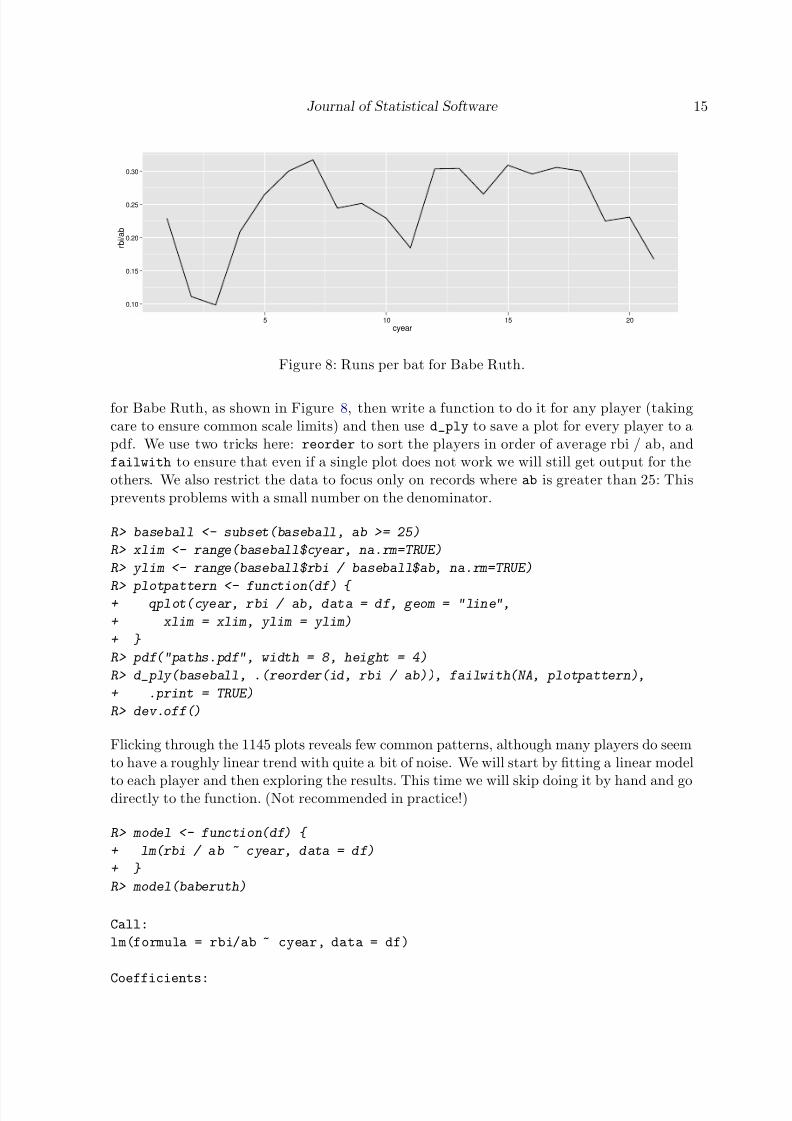
Figure 8: Runs per bat for Babe Ruth.

for Babe Ruth, as shown in Figure 8, then write a function to do it for any player (takingcare to ensure common scale limits) and then use d_ply to save a plot for every player to apdf. We use two tricks here: reorder to sort the players in order of average rbi / ab, andfailwith to ensure that even if a single plot does not work we will still get output for theothers. We also restrict the data to focus only on records where ab is greater than 25: Thisprevents problems with a small number on the denominator.

R> baseball <- subset(baseball, ab >= 25)

R> xlim <- range(baseball$cyear, na.rm=TRUE)

R> ylim <- range(baseball$rbi / baseball$ab, na.rm=TRUE)

R> plotpattern <- function(df) { + qplot(cyear, rbi / ab, data = df, geom = "line",

+ xlim = xlim, ylim = ylim)

+ }

R> pdf("paths.pdf", width = 8, height = 4)

R> d_ply(baseball, .(reorder(id, rbi / ab)), failwith(NA, plotpattern),

+ .print = TRUE)

R> dev.off()

Flicking through the 1145 plots reveals few common patterns, although many players do seemto have a roughly linear trend with quite a bit of noise. We will start by fitting a linear model

to each player and then exploring the results. This time we will skip doing it by hand and godirectly to the function. (Not recommended in practice!)

R> model <- function(df) {

+ lm(rbi / ab ~ cyear, data = df)

+ }

R> model(baberuth)

Call:

lm(formula = rbi/ab ~ cyear, data = df)

Coefficients:




id intercept slope rsquare

aaronha01 0.18 0.00 0.00

abernte02 0.00 0.00adairje01 0.09 −0.00 0.01adamsba01 0.06 0.00 0.03adamsbo03 0.09 −0.00 0.11adcocjo01 0.15 0.00 0.23

Table 4: The first few rows of the bcoefs data frame. Note that the player ids from theoriginal data have been preserved.

(Intercept) cyear

0.20797 0.00332

R> bmodels <- dlply(baseball, .(id), model)

Now we have a list of 1145 models, one for each player. To do something interesting withthese, we need to extract some summary statistics. We will extract the coefficients of themodel (the slope and intercept), and a measure of model fit (R2) so we can ensure we arenot drawing conclusions based on models that fit the data very poorly. The first few rows of coef are shown in Table 4.

R> rsq <- function(x) summary(x)$r.squared

R> bcoefs <- ldply(bmodels, function(x) c(coef(x), rsquare = rsq(x)))

R> names(bcoefs)[2:3] <- c("intercept", "slope")

Figure 9 displays the distribution of R2 across the models. The models generally do a verybad job of fitting the data, although there are few with an R2 very close to 1. We can see thedata that generated these perfect fits by merging the coefficients with the original data, andthen selecting records with an R2 of 1:

R> baseballcoef <- merge(baseball, bcoefs, by = "id")

R> subset(baseballcoef, rsquare > 0.999)$id

[1] "bannifl01" "bannifl01" "bedrost01" "bedrost01" "burbada01" "burbada01"

[7] "carrocl02" "carrocl02" "cookde01" "cookde01" "davisma01" "davisma01"[13] "jacksgr01" "jacksgr01" "lindbpa01" "lindbpa01" "oliveda02" "oliveda02"

[19] "penaal01" "penaal01" "powerte01" "powerte01" "splitpa01" "splitpa01"

[25] "violafr01" "violafr01" "wakefti01" "wakefti01" "weathda01" "weathda01"

[31] "woodwi01" "woodwi01"

All the models with a perfect fit only have two data points. Figure 10 is another attempt tosummarize the models. These plots show a negative correlation between slope and intercept,and the particularly bad models have estimates for both values close to 0. This concludes thebaseball player case study, which used used ddply, d_ply, dlply and ldply. Our statisticalanalysis was not very sophisticated, but the tools of plyr made it very easy to work at the

player level. This is an sensible first step when creating a hierarchical model.




rsquare

c o u n t

0

50

100

150

200

0.0 0.2 0.4 0.6 0.8 1.0

Figure 9: Histogram of model R2 with bin width of 0.05. Most models fit very poorly!

slope

i n t e r c e p t

−0.1

0.0

0.1

0.2

−0.04−0.020.000.020.040.060.08

rsquare

0.00

0.25

0.50

0.75

1.00

slope

i n t e r c e p t

−0.10

−0.05

0.00

0.05

0.10

0.15

0.20

0.25

−0.010 −0.005 0.000 0.005 0.010

rsquare

0.00

0.25

0.50

0.75

1.00

Figure 10: A scatterplot of model intercept and slope, with one point for each model (player).The size of the points is proportional to the R2 of the model. Vertical and horizontal linesemphasize the x and y origins.

5.2. Case study: Ozone

In this case study we will analyze a 3d array that records ozone levels over a 24× 24 spatial gridat 72 time points (Hobbs, Wickham, Hofmann, and Cook 2010). This produces a 24× 24× 723d array, containing a total of 41 472 data points. Figure 11 shows one way of displaying thisdata. Conditional on spatial location, each star glyph shows the evolution of ozone levels foreach of the 72 months (6 years, 1995–2000). The construction of the glyph is described inFigure 12; it is basically a time series in polar coordinates. The striking seasonal patternsmake it difficult to see if there are any long-term changes. In this case study, we will explorehow to separate out and visualize the seasonal effects. Again we will start with the simplestcase: A single time point, from location (1, 1). Figure 13 displays this in two ways: As a

single line over time, or a line for each year over the months. This plot illustrates the striking




−20

−10

0

10

20

30

−110 −85 −60

Figure 11: Star glyphs showing variation in ozone over time at each spatial location.

seasonal variation at this time point. The following code sets up some useful variables.

R> value <- ozone[1, 1, ]

R> time <- 1:72 / 12

R> month.abbr <- c("Jan", "Feb", "Mar", "Apr", "May",

+ "Jun", "Jul", "Aug", "Sep", "Oct", "Nov", "Dec")

R> month <- factor(rep(month.abbr, length = 72), levels = month.abbr)

R> year <- rep(1:6, each = 12)

We are going to use a quick and dirty method to remove the seasonal variation: Residuals

from a robust linear model (Venables and Ripley 2002) that predicts the amount of ozone




0.0

0.2

0.4

0.6

0.8

1.0

q

0.0 0.2 0.4 0.6 0.8 1.0

−1.0

−0.5

0.0

0.5

1.0

q

q

−0.5 0.0 0.5

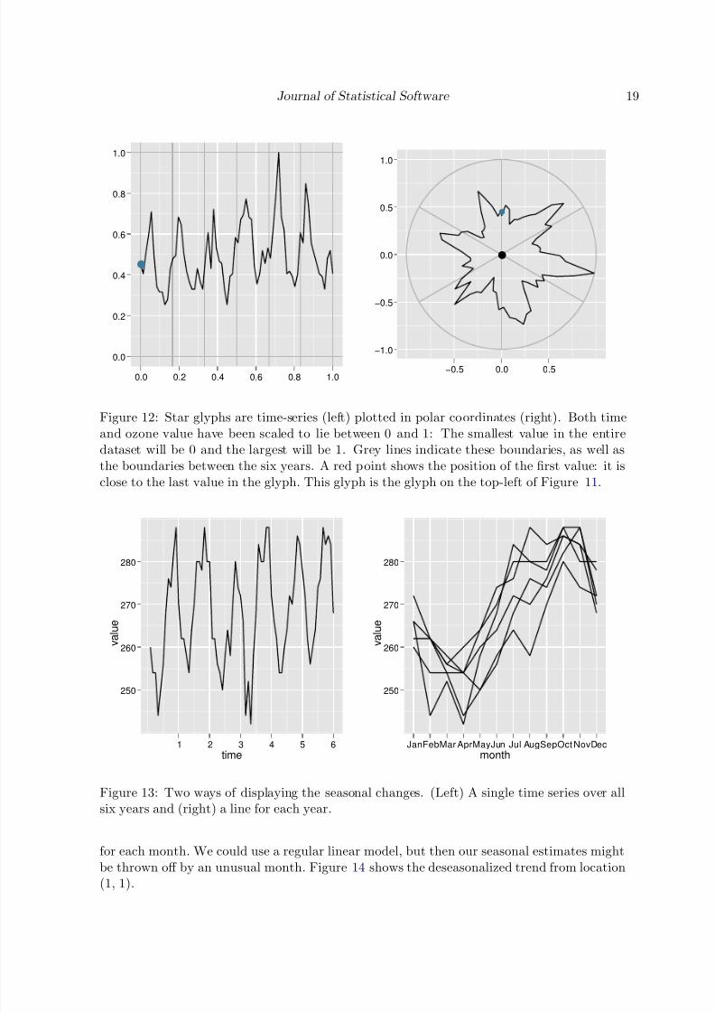
Figure 12: Star glyphs are time-series (left) plotted in polar coordinates (right). Both timeand ozone value have been scaled to lie between 0 and 1: The smallest value in the entiredataset will be 0 and the largest will be 1. Grey lines indicate these boundaries, as well asthe boundaries between the six years. A red point shows the position of the first value: it isclose to the last value in the glyph. This glyph is the glyph on the top-left of Figure 11.

time

v a l u e

250

260

270

280

1 2 3 4 5 6

month

v a l u e

250

260

270

280

JanFebMar AprMayJun Jul AugSepOct NovDec

Figure 13: Two ways of displaying the seasonal changes. (Left) A single time series over allsix years and (right) a line for each year.

for each month. We could use a regular linear model, but then our seasonal estimates mightbe thrown off by an unusual month. Figure 14 shows the deseasonalized trend from location

(1, 1).




time

r e s i d ( d e s e a s 1 )

−15

−10

−5

0

5

10

1 2 3 4 5 6

month

u n n a m e ( c o e f ( d e s e a s 1 ) )

255

260

265

270

275

280

285

JanFebMar AprMayJun Jul AugSepOct NovDec

Figure 14: Deseasonalized ozone trends. (Left) Deseasonalized trend over six years. (Right)Estimates of seasonal effects. Compare to Figure 13.

R> library("MASS")

R> deseas1 <- rlm(value ~ month - 1)

R> summary(deseas1)

Call: rlm(formula = value ~ month - 1)Residuals:

Min 1Q Median 3Q Max

-18.7 -3.3 1.0 3.0 11.3

Coefficients:

Value Std. Error t value

monthJan 264.40 2.75 96.19

monthFeb 259.20 2.75 94.30

monthMar 255.00 2.75 92.77

monthApr 252.00 2.75 91.68

monthMay 258.51 2.75 94.05 monthJun 265.34 2.75 96.53

monthJul 274.00 2.75 99.68

monthAug 276.67 2.75 100.66

monthSep 277.00 2.75 100.78

monthOct 285.00 2.75 103.69

monthNov 283.60 2.75 103.18

monthDec 273.20 2.75 99.39

Residual standard error: 4.45 on 60 degrees of freedom

R> coef(deseas1)




monthJan monthFeb monthMar monthApr monthMay monthJun monthJul monthAug

264 259 255 252 259 265 274 277

monthSep monthOct monthNov monthDec277 285 284 273

We next turn this into a function and fit the model to each spatial location. This does takea little while, but we are fitting 576 models! As is common when fitting large numbers of models, some of the models does not fit very well, and rlm() does not converge. We figureout where these lie by looking at the converged attribute for each model. In a real analysisit would be important to figure why these locations are troublesome and deal with themappropriately, but here we will just ignore them.

R> deseasf <- function(value) rlm(value ~ month - 1, maxit = 50)

R> models <- alply(ozone, 1:2, deseasf)

Warning message: rlm failed to converge in 50 steps







R> failed <- laply(models, function(x) !x$converged)

From those models we extract the deseasonalized values (the residuals) and the seasonal coef-ficients. Looking at the dimensionality we see that they are in the same format as the originaldata. We also carefully label the new dimensions. This is important: Just as data framesshould have descriptive variable names, arrays should always have descriptive dimension la-bels.

R> coefs <- laply(models, coef)

R> dimnames(coefs)[[3]] <- month.abbr

R> names(dimnames(coefs))[3] <- "month"

R> deseas <- laply(models, resid)

R> dimnames(deseas)[[3]] <- 1:72

R> names(dimnames(deseas))[3] <- "time"

R> dim(coefs)

[1] 24 24 12

R> dim(deseas)

[1] 24 24 72

We now have a lot of data to try and understand: For each of the 576 locations we have

12 estimates of monthly effects, and 72 residuals. There are many different ways we could




−20

−10

0

10

20

30

−110 −85 −60

avg

250

260

270

280

290

300

310

Figure 15: Star glyphs showing seasonal variation. Each star shows the twelve estimates of monthly seasonal effects, standardized to have maximum one. This focuses on the overall

pattern of changes, rather than the absolute values, given by the glyph colour. Note thestrong spatial correlation: Nearby glyphs have similar shapes.

visualize this data. Figures 15 and 16 visualize these results with star glyph plots. Forplotting, it is more convenient to have the data in data frames. There are a few different waysto do this: We can convert from the 3d array to a data frame with melt() from the reshape

package, or use ldply() instead of laply(). For this example, we will use a combinationof these techniques. We will convert the original array to a data frame, add on some usefulcolumns, and then perform the same steps as above with this new format. Notice how oureffort labeling the array dimensions pays off with informative column names in coefs_df:

lat, long and month.




−20

−10

0

10

20

30

−110 −85 −60

Figure 16: Star glyphs showing deseasonalized trends. Each star shows six years of data,with seasonal trend removed. This plot contains a lot of data—over 40,000 observations—

and rewards detailed study. Looking at a printed version also helps as the resolution of aprinter (600 dpi) is much higher than that of the screen (∼100 dpi). Interesting featuresinclude the higher variability in the North, locations in the mountains of South America witha large difference between starting and ending temperatures, and an unusual month commonto many of the locations in the Pacific.

R> coefs_df <- melt(coefs)

R> head(coefs_df)

lat long month value

1 -21.2 -114 Jan 264




2 -18.7 -114 Jan 261

3 -16.2 -114 Jan 261

4 -13.7 -114 Jan 2595 -11.2 -114 Jan 256

6 -8.7 -114 Jan 255

R> coefs_df <- ddply(coefs_df, .(lat, long), transform,

+ avg = mean(value),

+ std = value / max(value)

+ )

R> head(coefs_df)

lat long month value avg std

1 -21.2 -114 Jan 264 269 0.9282 -21.2 -114 Feb 259 269 0.909

3 -21.2 -114 Mar 255 269 0.895

4 -21.2 -114 Apr 252 269 0.884

5 -21.2 -114 May 259 269 0.907

6 -21.2 -114 Jun 265 269 0.931

R> deseas_df <- melt(deseas)

R> head(deseas_df)

lat long time value

1 -21.2 -114 1 -4.40

2 -18.7 -114 1 -3.33

3 -16.2 -114 1 -2.96

4 -13.7 -114 1 -5.00

5 -11.2 -114 1 -4.00

6 -8.7 -114 1 -3.00

The star glyphs show temporal patterns conditioned on location. We can also look at spatialpattern conditional on time. One way to do this is to draw tile plots where each cell of the24× 24 grid is colored according to its value. The following code sets up a function with

constant scales to do that. Figure 17 shows the spatial variation of seasonal coefficients forJanuary and July.

R> coef_limits <- range(coefs_df$value)

R> coef_mid <- mean(coefs_df$value)

R> monthsurface <- function(mon) {

+ df <- subset(coefs_df, month == mon)

+ qplot(long, lat, data = df, fill = value, geom="tile") +

+ scale_fill_gradient(limits = coef_limits,

+ low = brightblue, high = "yellow") +

+ map + opts(aspect.ratio = 1)

+ }




−20

−10

0

10

20

30

−110 −85 −60

value

260

280

300

320

340

−20

−10

0

10

20

30

−110 −85 −60

value

260

280

300

320

340

Figure 17: Tile plots of coefficients for January (left) and July (right).

We could do the same thing for the values themselves, but we would probably want to makean animation rather than looking at all 72 plots individually. The *_ply functions are usefulfor making animations because we are only calling the plotting function for its side effects,not because we are interested in its value.

R> pdf("ozone-animation.pdf", width = 8, height = 8)R> l_ply(month.abbr, monthsurface, .print = TRUE)

R> dev.off()

5.3. Other uses

The transform(), summarise() and subset() functions work well in combination with plyr.Transform makes it very easy to perform randomization within groups. For example thefollowing expression returns a data frame like coefs_df, but with the values in the time

column randomized within each latitude/longitude grouping:

ddply(coefs_df, .(lat, long), transform, time = sample(time))

This technique is useful for performing block bootstrapping and other related permutationtests, and is related to the ave function in base R. Scaling variables within a group is alsotrivial:

ddply(coefs_df, .(lat, long), transform, value = scale(value))

We can create group-wise summaries with summarise() (or summarize()). For example, itis easy to summarize the range of ozone at each location:

ddply(coefs_df, .(lat, long), summarise,

ozone_min = min(value), ozone_max = max(ozone))




Base function Input Output plyr function

aggregate d d ddply + colwise

apply a a/l aaply / alplyby d l dlply

lapply l l llply

mapply a a/l maply / mlply

replicate r a/l raply / rlply

sapply l a laply

Table 5: Mapping between apply functions and plyr functions.

Group-wise subsetting is easy with subset(). For example, if we wanted to extract theobservation in each group with the lowest value ozone of ozone, it is just as easy:

ddply(coefs_df, .(lat, long), subset, value == min(value))

For simulations, mdply() can be very useful, because it is easy to generate a grid of pa-rameter values and then evaluate them. This can also be useful when testing many possiblecombinations to input to a function.

mdply(expand.grid(mean = 1:5, sd = 1:5), as.data.frame(rnorm), n = 10)

6. Related work

There are a number of other approaches to solving the problems that plyr solves. You canalways use loops, but loops create a lot of book-keeping code that obscures the intent of youralgorithm. This section describes other high-level approaches similar to plyr.

Table 5 describes the functions in base R that work similarly to functions in plyr. The built-in

R functions focus mainly on arrays and lists, not data frames, and most attempt to returnan atomic data structure if possible, and if not, a list. This ambiguity of the output type isfine for interactive use, but does make programming with these functions tricky. Comparedto aaply, apply returns the new dimensions first, rather than last, which means it is not

idempotent when used with the identity function. In contrast, aaply(x, a, identity)== aperm(x, unique(c(a, seq_along(dim(x))))) for all a.

Related functions tapply and sweep have no corresponding function in plyr, and remainuseful. merge is useful for combining summaries with the original data.

Contributed packages also tackle this problem:

The doBy (Højsgaard 2006, 2011) package provides versions of order, sample, split,subset, summary and transform that make it easy to perform each of these operationson subsets of data frames, joining the results back into a data frame. These functionsare rather like a specialized version of ddply with a formula based interface, which,

particularly for summary, makes it easy to only operate on selected columns.




The abind (Plate and Heiberger 2011) package provides the abind() function which canbe used to construct multidimensional arrays in a similar way to the *aply functions.

The gdata (Warnes 2010) package contains a bundle of helpful data manipulation func-tions, including frameApply which works like ddply or dlply depending on its argu-ments.

The scope (Bergsma 2007) package provides scope, scoop, skim, score and probe

which provide a composable set of functions for operating symbolically on subsets of data frames.

The reshape (Wickham 2007) package is similar to Excel pivot tables and provides toolsfor rearranging matrices and data frames. The cast function in the reshape package isclosely related to aaply.

The sqldf (Grothendieck 2010) package allows you to use SQL commands with R dataframes. This gives the user access to a powerful set-based data access language.

7. Conclusion

Speed-wise plyr is competitive with R for small to moderate sized datasets, and generallya little faster for large datasets split by many different values. It is more memory-efficientthan the naive split-apply-combine approach because plyr is careful not to make an extracopy of the data in the split step. Further efficiency gains are possible, particularly by

implementing key parts C for maximum speed and memory efficiency. The basic algorithmof plyr is trivially parallelizable, and future versions will integrate with the foreach package(REvolution Computing 2009) to make use of multiple cores and multiple machines.

More generally, what are other common strategies used in data analysis? How can we identifythese strategies and then develop software to support them? It is difficult to step back andidentify these patterns as trivial details may obscure the common components; it took fouryears of thinking about related problems before I recognized this split-apply-combine strategy.However, the task is important because the patterns are so useful. Personally, identifying thesplit-apply-combine strategy has made it much easier for me to solve common data analysisproblems, and I have also found useful when teaching others how to do data analysis.

8. Acknowledgments

Thanks go to Norman Josephy, Austin F. Frank, Antony Unwin, Joseph Voelkel, Erik Iverson,and Jean-Olivier Irisson for their comments on early versions of this paper.

References

Bergsma T (2007). scope: Data Manipulation Using Arbitrary Row and Column Crite-ria . R package version 2.2, URL http://CRAN.R-project.org/src/contrib/Archive/

scope/.

http://cran.r-project.org/src/contrib/Archive/scope/








Dalgaard P (2001). “A Primer on the R-Tcl/Tk Package.” R News , 1(3), 27–31. URLhttp://CRAN.R-project.org/doc/Rnews/ .

Friendly M, Fox J (1994). “Using APL2 to Create an Object-Oriented Environment for Sta-tistical Computation.” Journal of Computational and Graphical Statistics , 3, 387–407.

Grothendieck G (2010). sqldf : Perform SQL Selects on R Data Frames . R package version0.3-5, URL http://CRAN.R-project.org/package=sqldf .

Hobbs J, Wickham H, Hofmann H, Cook D (2010). “Glaciers Melt as Mountains Warm: AGraphical Case Study.” Computational Statistics , 25(4), 569–586. Special issue for ASAStatistical Computing and Graphics Data Expo 2007.

Højsgaard S (2006). “The doBy Package.” R News , 6(2), 47–49. URL http://CRAN.R-project.org/doc/Rnews/ .

Højsgaard S (2011). doBy : Groupwise Summary Statistics, General Linear Contrasts,LSMEANS (Least-Squares-Means), and Other Utilities . R package version 4.2.3. Withcontributions from Ulrich Halekoh, Jim Robison-Cox, Kevin Wright, Alessandro A. Leidi,URL http://CRAN.R-project.org/package=doBy .

Plate T, Heiberger R (2011). abind : Combine Multi-dimensional Arrays . R package ver-sion 1.3-0, URL http://CRAN.R-project.org/package=abind .

R Development Core Team (2010). R : A Language and Environment for Statistical Computing .R Foundation for Statistical Computing, Vienna, Austria. ISBN 3-900051-07-0, URL http:

//www.R-project.org/.

REvolution Computing (2009). foreach : Foreach looping construct for R . R package version1.3.0, URL http://CRAN.R-project.org/package=foreach .

Sarkar D (2008). lattice: Multivariate Data Visualization with R . Springer-Verlag, New York.

Venables WN, Ripley BD (2002). Modern Applied Statistics with S . 4th edition. Springer-Verlag, New York.

Warnes GR (2010). gdata : Various R Programming Tools for Data Manipulation . R packageversion 2.8.0. With contributions from Ben Bolker, Gregor Gorjanc, Gabor Grothendieck,Ales Korosec, Thomas Lumley, Don MacQueen, Arni Magnusson, Jim Rogers, and others,URL http://CRAN.R-project.org/package=gdata .

Wickham H (2007). “Reshaping data with the reshape package.” Journal of Statistical Soft-ware , 21(12), 1–20. URL http://www.jstatsoft.org/v21/i12/paper .

Wickham H (2010). ggplot2 : An Implementation of the Grammar of Graphics . R package

version 0.8.7, URL http://CRAN.R-project.org/package=ggplot2 .

http://cran.r-project.org/doc/Rnews/


http://cran.r-project.org/package=sqldf



http://cran.r-project.org/package=doBy


http://cran.r-project.org/package=abind


http://www.r-project.org/


http://cran.r-project.org/package=foreach

http://cran.r-project.org/package=gdata


http://www.jstatsoft.org/v21/i12/paper

http://cran.r-project.org/package=ggplot2

http://cran.r-project.org/package=ggplot2

http://www.jstatsoft.org/v21/i12/paper


http://cran.r-project.org/package=foreach







http://cran.r-project.org/package=sqldf





Affiliation:

Hadley Wickham

Rice UniversityHouston, TX 77251-1892, United States of AmericaE-mail: [email protected]

URL: http://had.co.nz/

Journal of Statistical Software http://www.jstatsoft.org/

published by the American Statistical Association http://www.amstat.org/

Volume 40, Issue 1 Submitted: 2009-09-24April 2011 Accepted: 2010-12-27

mailto:[email protected]

http://had.co.nz/


http://www.amstat.org/

http://www.amstat.org/


http://had.co.nz/

mailto:[email protected]

wickham - jss11 - plyr

Documents