www.SandV.com8 SOUND & VIBRATION/APRIL 2016

Wideband Acoustical Holography

All patch, near-field acoustical holography (NAH) methods like statistically optimized NAH and the equivalent-source method are limited to relatively low frequencies, where the average ar-ray inter-element spacing is less than half a wavelength, while beamforming provides useful resolution only at medium-to-high frequencies. With adequate array design, both methods can be used with the same array. But for holography to provide good low-frequency resolution, a small measurement distance must be used, while beamforming requires a longer distance to limit side-lobe issues. Wideband holography was developed to overcome that practical conflict. Only a single measurement is needed at a relatively short distance, and a single result is obtained covering the full frequency range. The underlying problem solved is that at high frequencies, the microphone spacing is too large to meet the spatial sampling criterion. So there is no unique reconstruc-tion of the sound field. A reconstruction must therefore have a built-in “preference” for specific forms of the sound field. Doing just a least-squares solution will result in reconstructed sound fields, with sound pressure equal to the measured pressure at the microphones but very low elsewhere. By building in a preference for compact sources, a smoother form of the reconstructed sound field is enforced.

Near-field acoustical holography (NAH) is based on performing 2D spatial discrete Fourier transforms (DFT);1 therefore the method requires a regular mesh of measurement positions. To avoid spatial aliasing problems, the mesh spacing must be somewhat less than half the acoustic wavelength. In practice, this requirement sets a serious limitation on the upper frequency limit.

Some patch NAH methods, for example the equivalent-source method (ESM)2 and the statistically optimized NAH (SONAH),3 can work with irregular microphone array geometries, but still require an array element spacing of less than half the wavelength. As described in Reference 4, this allows the use of irregular arrays that are actually designed for use with beamforming.

Typically, good performance with beamforming can be achieved up to frequencies where the average array inter-element spacing is two to three wavelengths. A practical issue with such a solution is that the patch NAH method requires measurement at a short distance to provide good resolution at low frequencies, while beamforming requires a medium-to-long distance to keep side lobes at low levels. So for optimal wide-band performance, two measurements must be taken at different distances, and separate types of processing must be used with the two measurements. This makes it difficult to combine the results into a single result covering the combined frequency range.

The rather new compressive sensing (CS) methods,5 have started making it possible to use irregular-array geometries for holography up to frequencies where the average array interelement spacing is significantly larger than half the wavelength. In general, these methods allow reconstruction of a signal from sparse irregular samples under the condition that the signal can be (approximately) represented by a sparse subset of expansion functions in some domain. That is, with the expansion coefficients (amplitudes) of most functions equal to zero.

The underlying problem solved is that at high frequencies, the microphone spacing is too large to meet the spatial sampling criterion, so there is no unique reconstruction of the sound field. A reconstruction must therefore have a built-in “preference” for specific forms of the sound field. Doing just a least-squares solu-tion will result in reconstructed sound fields with sound pressure equal to the measured pressure at the microphones but very low elsewhere. By building in a preference for compact sources, a smoother form of the reconstructed sound field is enforced.

This article describes a new method called wideband holography (WBH), which is covered by a pending patent.6 The method is

similar to one previously published.7 However, instead of apply-ing a 1-norm penalty to enforce sparsity in the monopole source model, WBH uses a dedicated iterative solver that enforces sparsity in a different way.

TheoryInput data for patch holography processing is typically obtained

by simultaneous acquisition with an array of M microphones, indexed by m = 1,2…,+M, followed by averaging of the M × M element cross-power spectral matrix between the microphones. For the subsequent description, we arbitrarily select a single high-frequency line f with associated cross-power matrix G. An eigenvector/eigenvalue factorization is then performed of that Hermitian, positive-semi-definite matrix G:

V being a unitary matrix with the columns containing the eigen-vectors vµ, µ = 1,2…,M, and S a diagonal matrix with the real non-negative eigenvalues sµ on the diagonal. Based on the factorization in Eq. 1, the principal component vectors pµ can be calculated as:

Just like ESM and SONAH, the WBH algorithm is applied indepen-dently to each of these principal components, and subsequently the output is added on a power basis, since the components rep-resent incoherent parts of the sound field. So for the subsequent description we consider a single principal component, and we skip the index µ, meaning that input data are a single vector p with measured complex sound pressure values for all microphones.

WBH uses a source model in terms of a set of elementary sources or wave functions and solves an inverse problem to identify the complex amplitudes of all elementary sources. The source model then applies for 3D reconstruction of the sound field. Here we will consider only the case where the source model is a mesh of monopole point sources retracted to be behind/inside the real/specified source surface, i.e., similar to the model applied in ESM.2 With Ami representing the sound pressure at microphone m due to a unit excitation of monopole number i, the requirement that the modelled sound pressure at microphone m must equal the measured pressure pm can be written as:

Here, I is the number of point sources, and qi, i = 1,2…,I, are the complex amplitudes of these sources. Eq. 3 can be rewritten in matrix-vector notation as:

where A is an M × I matrix containing the quantities Ami, and q is a vector with elements qi. In compressive-sensing terminology, the matrix A is called the sensing matrix.

When doing standard patch holography calculations using ESM, Tikhonov regularization is typically applied to stabilize the minimization of the residual vector. This is done by adding a penalty proportional to the 2-norm of the solution vector when minimizing the residual norm:

A very important property of that problem is that it has the simple analytic solution:

where I is a unit diagonal matrix, and H represents Hermitian transpose.

(1)G = VSVH

(2)p vm m m = s

(3)p A qm m ii

n

==Â

1

(4)p Aq=

(6)q A A I A p= +ÈÎ ˘̊-H Hq 2 1

S. Gade, J. Hald and K. B. Ginn, Brüel & Kjær Sound & Vibration Measurements A/S, Nærum, Denmark

(5)Minimize � � � �p Aq qq

- +22 2

22q

www.SandV.com SOUND & VIBRATION/APRIL 2016 9

A suitable value of the regularization parameter q for given input data p can be identified automatically, for example, by use of generalized cross validation (GCV).8 When using a specific ir-regular array well above the frequency of half wavelength average microphone spacing, the system of linear equations in Eq. 4 is in general strongly underdetermined, because the monopole mesh must have spacing less than half the wavelength; that is, much finer than the microphone grid.

During the minimization in Eq. 5, the undetermined degrees of freedom will be used to minimize the 2-norm of the solution vec-tor. The consequence is a reconstructed sound field that matches the measured pressure values at the microphone positions but with minimum sound pressure elsewhere. Estimates of sound power, for example, will be much too low. Another effect is ghost sources, because available measured data is far from determining a unique solution.

A main idea behind the WBH method is to remove/suppress the ghost sources associated with the real sources in an iterative solu-tion process, starting with the strongest real sources. For a detailed mathematical description, see Reference 9. In the following, we will just highlight some of the most important points.

In the first step of the steepest-descent iteration process, a num-ber of real as well as ghost sources are introduced/identified, but when using irregular array geometries, the ghost images will in general be weaker than the strongest real source(s). We can therefore suppress the ghost sources by setting all components in the first iteration step below a certain threshold to zero. The threshold is computed as being a number of decibels below the amplitude of the largest element.

The dynamic range of retained-source amplitudes, Dk, is updated during the iteration steps k so that an increasing dynamic range of sources will be included, typically:

In the limiting case when Dkƕ for kƕ, the dynamic range limitation is gradually removed. However, the iteration can be stopped when:

where Dmax is an upper limit on Dk or when some other stopping criteria are fulfilled. In general, the source model may not be able to completely represent the measured pressure data, but the fol-lowing values have been found to work generally very well: D0 = 0.1 dB, DD = 1.0 dB and Dmax = 60 dB.

The upper-limiting dynamic range Dmax can be changed to match the quality of data, but the choice does not seem to be critical. We have found that Dmax = 60 dB supports the identification of weak sources, even when measurements are slightly noisy. Larger values do not seem to improve much. Smaller values may be required for very noisy data.

Starting with only 0.1 dB, dynamic range means that only the very strongest source(s) will be retained, while all related ghost sources will be removed. When we use the dynamic- range-limited source vector as the starting point for the next iteration, the components of the residual vector related to the very strongest source(s) have been reduced; therefore the related ghost sources have been reduced correspondingly. Increasing the dynamic range will then cause the next level of real sources to be included, while suppressing the related ghost sources, etc. Another aspect is that a minimum number of the point sources of the model will be as-signed an amplitude different from zero, enforcing effectively a sparse solution. After the termination of the above algorithm based on steepest descent directions, a good estimate of the basic source distribution has been achieved.

The WBH algorithm, which enforces a maximum degree of sparsity in the source distribution, has been found to work well at high frequencies when a suitable array is used at a not-too-small measurement distance. At low frequencies, however, WBH easily leads to misleading results when two compact sources are so close that available data do not support a resolution of the two with beamforming. In that case, the WBH algorithm (and perhaps other sparsity-enforcing algorithms) will often identify a single compact

source at a position between the two real sources. So the user might be drawing wrong conclusions about the root cause of the noise.

Use of the traditional Tikhonov regularization of Eq. 6 (a standard ESM algorithm) will in that case typically show a single large ob-long source area covering both of the two real sources (see Figure 6). To minimize the risk of misleading results, it is recommended to use the standard ESM solution up to a transition frequency at approximately 0.7 times the frequency of a half wavelength average array inter-element spacing (with spacing ≈0.35l), and above that transition frequency switch to the use of the iterative solver WBH.

Array DesignAs described earlier, the method here follows the principles of

compressive sensing, based on measurements with a random or pseudo-random array geometry in combination with an assumed sparsity of the coefficient vector of the source model.

The principle of circular, pseudo-random array geometry used in the real and simulated measurements is shown in Figure 1. It has 12 microphones uniformly distributed in a sector. There are an odd number of sectors, typically 3, 5 or 7 sectors, which are respectively 36, 60 and 84 microphones in the array. For the simu-lated measurements, a 1-m diameter array with 60 microphones was used, so the average element spacing is approximately 12 cm, implying a low-to-high transition frequency close to 1 kHz (0.35l).

The geometry, which consists of five identical angular sectors, has been optimized for beamforming measurements up to 6 kHz as described in Reference 4. For most of the real measurements, a 0.45-m diameter array with 36 microphones was used, so the average element spacing is approximately 6.6 cm, implying a transition frequency close to 2.3 kHz. The geometry, which in this case consists of three identical angular sectors, has been optimized for beamforming measurements up to 14 kHz.

An important finding from simulated measurements with the chosen array design is that the measurement distance should not be shorter than approximately twice the average microphone spacing for the method to work well at the highest frequencies. A factor of three is even better. Using the longer measurement distance with WBH has the effect of reducing the difference between the direc-

(7)D D Dk k+ = +1 D

(8)D Dk + >1 max

Figure 1. Planar pseudo-random microphone array geometries: (a) five sec-tors, 60 elements; and (b) three sectors, 36 elements.

Figure 2. Contour plots of sound intensity in source plane; 24 cm in front of array plane; display range is 30 dB with 3 dB contour interval; same scale used in all plots. (a) True, (b) Tikhonov, (c) WBH – iterative solver.

Figure 3. Contour plots of sound pressure in array plane; display range is 15 dB with 1 dB contour interval; same scale in all plots. (a) True, (b) Tikhonov, (c) WBH – iterative solver.

www.SandV.com10 SOUND & VIBRATION/APRIL 2016

tion of arrival application and the WBH application.

Another view of this is the fact that each source in the WBH source model will expose the microphones over a wider area when the measurement distance is increased. To get acceptable low-frequency reso-lution, however, the distance should not be too great either, so the best overall distance seems to be around twice the

average array inter-element spacing.Note that the ESM/WBH (using ESM algorithm with Tikhonov

regularization up to a frequency corresponding to 0.35l of the microphone spacing and the WBH iterative regularization at higher frequencies) algorithm is a very tolerant approach with respect to measurement distance. Measurement may be done in the near field as well as in the far field, while keeping in mind that longer dis-tances improve high-frequency performance and shorter distances improve low-frequency performance. A good balance between high- and low-frequency performance is using a distance equal to two-to-three-times the microphone spacing.

Simulated MeasurementsThe aim of this simulated measurement is to demonstrate with

a very simple single monopole source configuration: • What happens if Tikhonov regularization is applied above the

frequency of half wavelength average array element spacing?• How much and what kind of improvement is achieved by apply-

ing WBH that is using the dedicated iterative solver?A monopole point source is located on the array axis at 28 cm

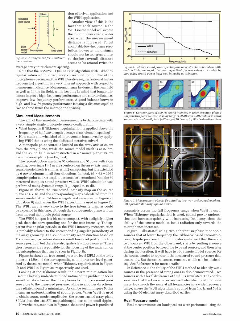
from the array plane, while the source-model mesh is at 27 cm, and the sound field in reconstructed in a “source plane” 24 cm from the array plane (see Figure 4).

The reconstruction mesh has 51 columns and 51 rows with 2-cm spacing, covering a 1 × 1 m area centered on the array axis, and the source-model mesh is similar, with 2-cm spacing, but it is extended by 6 rows/columns in all four directions. In total, 63 × 63 = 3969 complex point-source amplitudes must be determined from the 60 measured complex sound pressure values. WBH calculation was performed using dynamic range Dmax equal to 40 dB.

Figure 2a shows the true sound intensity map on the source plane at 4 kHz, and the corresponding maps calculated from the source model. When Tikhonov regularization is used in Figure 2b (Equation 6) and, when the WBH algorithm is used in Figure 2c. The WBH map is very close to the true intensity map, as could be expected in this case, although the source-model plane is 1 cm from the real monopole point source.

The WBH hotspot is a bit more compact, with a slightly higher peak than the corresponding one for the true intensity. The ap-parent five angular periods in the WBH intensity reconstruction is probably related to the corresponding angular periodicity of the array geometry. The sound intensity reconstruction based on Tikhonov regularization shows a small low-level peak at the true source position, but there are also quite a few ghost sources. These ghost sources are responsible for the focusing of the radiation on the microphones that can be seen in Figure 3b.

Figure 3a shows the true sound pressure level (SPL) on the array plane at 4 kHz and the corresponding sound pressure level gener-ated by the source model, when Tikhonov regularization in Figure 3b and WBH in Figure 3c, respectively, are used.

Looking at the Tikhonov result, the 2-norm minimization has used the heavily underdetermined nature of the problem to focus sound radiation toward the microphones to produce a sound pres-sure close to the measured pressure, while in all other directions, the radiated sound is minimized. As can be seen in Figure 5, this means an underestimation of sound power. When WBH is used to obtain source model amplitudes, the reconstructed array-plane SPL is close the true SPL map, although it has some small ripples.

Nevertheless, as shown in Figure 5, the sound power is predicted

accurately across the full frequency range when WBH is used. When Tikhonov regularization is used, sound power underes-timation increases quickly with increasing frequency, since the ability of the source model to focus radiation only towards the microphones increases.

Figure 6 illustrates using two coherent in-phase monopole sources that at lower frequency the Tikhonov based reconstruc-tion, despite poor resolution, indicates quite well that there are two sources. WBH, on the other hand, starts by putting a source at the center position between the two real sources, and then later during the iteration, it will have to add remote model sources for the source model to represent the measured sound pressure data accurately. But the central source remains, which can be mislead-ing. See Reference 9 for more details.

In Reference 9, the ability of the WBH method to identify weak sources in the presence of strong ones is also demonstrated. Two sources with a level difference of 10 dB is simulated. The conclu-sion was that the two sources are well identified, and the noise maps look much the same at all frequencies in a wide frequency range, where the WBH algorithm is applied from 1 kHz and 5 kHz using the 60-element array described earlier.

Real MeasurementsReal measurements on loudspeakers were performed using the

Figure 4. Arrangement for simulated measurement.

Figure 6. Contour plots of 400-Hz sound intensity in reconstruction plane 5 cm from two point sources; display range is 20 dB with 2-dB contour interval; same scale used in all plots. (a) True, (b) Tikhonov, (c) WBH – iterative solver.

Figure 7. Measurement object: Two similar, two-way active loudspeakers; left speaker standing upside-down.

Figure 5. Relative sound power spectra from reconstructions based on WBH and on Tikhonov regularization, respectively; power values calculated by area using sound power from true intensity as reference.

www.SandV.com SOUND & VIBRATION/APRIL 2016 11

array in Figure 1b. It has a diameter of 45 cm and an average element spacing of 6.6 cm. Classical combination is holography (SONAH) at a distance of 7 cm covering a frequency range of 150-2200 Hz, with a spatial resolution of 7 cm and beamforming at a 27 cm distance covering a frequency range of 2-15 kHz with a resolution of 0.7l and side-lobe suppression of 10 dB. The measurement object was a pair of two-way loudspeakers as shown in Figure 7, and the size of the total object was 45 x 45 cm, corresponding to the size of the array.

A wide range of measurements was performed to confirm the theory and the simulated measurements of WBH. Measurements were performed at distances of 7 cm, 14 cm, 21 cm (corresponding to 1, 2 and 3 times the inter-element spacing), and 45 cm, 90 cm and 135 cm (corresponding to 1, 2 and 3 times the array diameter). The loudspeakers were driven by correlated white noise (of equal strength and a 10 dB level difference) in one series of measurements and uncorrelated white noise (also of equal strength and a 10 dB level difference) in another series of measurements. Calculations at low frequencies using WBH and ESM (Tikhonov regularization) were also compared.

Only the results of a few representative and illustrative measure-ment are shown:

Measurement at 14 cm. A distance of 14 cm corresponds to twice the average inter-element spacing. This is the recommended (opti-mum) distance for WBH as mentioned earlier. Measurement results are shown in the following. First at high frequencies then followed by medium and low frequencies. All displays use a 15-dB display range showing calculations of sound intensity in the source plane. The frequency resolution is in one-third octave bands. A source model mesh spacing of 1.5 cm enables calculations up to 10 kHz.

Figure 8 compares WBH against delay-and-sum (DAS) beam-forming at high frequencies (5 kHz and 10 kHz) for a measurement distance of 14 cm using uncorrelated noise. DAS results show high

side-lobe levels due to the relatively short distance for a beam-forming calculation. WBH is clearly indicating the position of two sources within the display range of 15 dB without any artefacts. Only the high-frequency loudspeaker units are radiating sound at these frequencies.

At mid frequencies (Figure 9) we can see that WBH and SONAH algorithms perform equally well, or in this example, WBH performs slightly better than SONAH. At the loudspeaker cross-over fre-quency of 2 kHz, all four speakers are easily identified and at 600 Hz, only the low frequency loudspeaker units are radiating sound. DAS performance is rather poor at these frequencies.

The standard WBH implementation as mentioned earlier is us-ing Tikhonovs SVD-based regularization (standard ESM) at lower frequency (below the 0.35l limit) to avoid artefacts as shown in Figure 6c and only uses (as default) the iterative-based regulariza-tion method at higher frequencies. Using the software, it is possible to override this rule and use the iterative WBH regularization algorithm also at low frequencies. Figure 10 shows a comparison of the two approaches at low frequency.

Figure 10 shows the importance of using the standard EMS algorithm at low frequencies, but in some cases it might be useful to switch to the iterative approach at low frequencies as well, since it provides a more compact solution. This has to be used with care of course. Note that we see similar results when the speakers are driven by correlated noise, except that the iterative artefacts already appear at a higher frequency (approximately one octave higher).

Figure 8. High-frequency results, 14 cm distance. (a) 10 kHz – WBH, (b) 10 kHz – DAS, (c) 5 kHz – WBH, (d) 5 kHz – DAS.

Figure. 9 Mid-frequency results, 14 cm distance. (a) 2 kHz – SONAH, (b) 2 kHz – WBH, (c) 2 kHz – DAS, (d) 600 Hz – SONAH, (e) 600 Hz – WBH, (f) 600 Hz – DAS.

Figure 10. Low-frequency results, 14 cm distance. (a) 500 Hz – Tikhonov regularization, (b) 500 Hz – iterative solver, (c) 160 Hz – Tikhonov regular-ization, (d) 160 Hz – iterative solver.

Figure 11. High-frequency results, 90 cm distance. (a) 10 kHz – WBH, (b) 10 kHz – DAS, (c) 10 kHz – NNLS, (d) 5 kHz – WBH, (e) 5 kHz – DAS, (f) 5 kHz – NNLS, (g) 2.5 kHz – WBH, (h) 2.5 kHz – DAS, (i) 2.5 kHz – NNLS.

www.SandV.com12 SOUND & VIBRATION/APRIL 2016

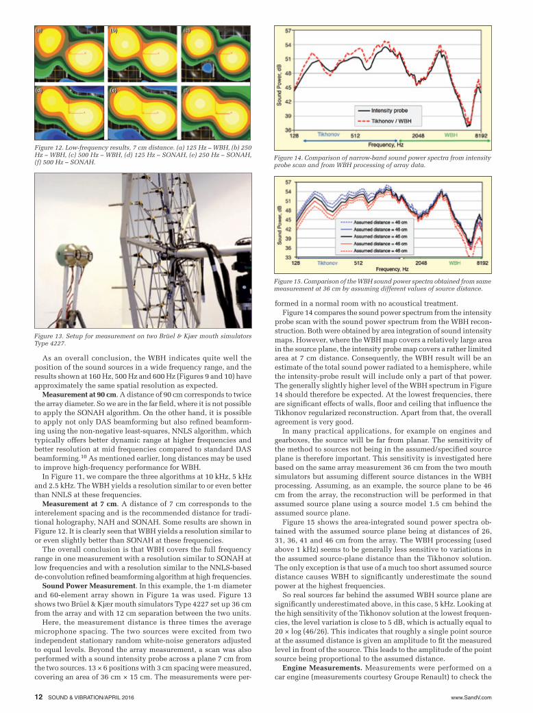
Figure 12. Low-frequency results, 7 cm distance. (a) 125 Hz – WBH, (b) 250 Hz – WBH, (c) 500 Hz – WBH, (d) 125 Hz – SONAH, (e) 250 Hz – SONAH, (f) 500 Hz – SONAH.

Figure 14. Comparison of narrow-band sound power spectra from intensity probe scan and from WBH processing of array data.

Figure 13. Setup for measurement on two Brüel & Kjær mouth simulators Type 4227.

Figure 15. Comparison of the WBH sound power spectra obtained from same measurement at 36 cm by assuming different values of source distance.

As an overall conclusion, the WBH indicates quite well the position of the sound sources in a wide frequency range, and the results shown at 160 Hz, 500 Hz and 600 Hz (Figures 9 and 10) have approximately the same spatial resolution as expected.

Measurement at 90 cm. A distance of 90 cm corresponds to twice the array diameter. So we are in the far field, where it is not possible to apply the SONAH algorithm. On the other hand, it is possible to apply not only DAS beamforming but also refined beamform-ing using the non-negative least-squares, NNLS algorithm, which typically offers better dynamic range at higher frequencies and better resolution at mid frequencies compared to standard DAS beamforming.10 As mentioned earlier, long distances may be used to improve high-frequency performance for WBH.

In Figure 11, we compare the three algorithms at 10 kHz, 5 kHz and 2.5 kHz. The WBH yields a resolution similar to or even better than NNLS at these frequencies.

Measurement at 7 cm. A distance of 7 cm corresponds to the interelement spacing and is the recommended distance for tradi-tional holography, NAH and SONAH. Some results are shown in Figure 12. It is clearly seen that WBH yields a resolution similar to or even slightly better than SONAH at these frequencies.

The overall conclusion is that WBH covers the full frequency range in one measurement with a resolution similar to SONAH at low frequencies and with a resolution similar to the NNLS-based de-convolution refined beamforming algorithm at high frequencies.

Sound Power Measurement. In this example, the 1-m diameter and 60-element array shown in Figure 1a was used. Figure 13 shows two Brüel & Kjær mouth simulators Type 4227 set up 36 cm from the array and with 12 cm separation between the two units.

Here, the measurement distance is three times the average microphone spacing. The two sources were excited from two independent stationary random white-noise generators adjusted to equal levels. Beyond the array measurement, a scan was also performed with a sound intensity probe across a plane 7 cm from the two sources. 13 × 6 positions with 3 cm spacing were measured, covering an area of 36 cm × 15 cm. The measurements were per-

formed in a normal room with no acoustical treatment.Figure 14 compares the sound power spectrum from the intensity

probe scan with the sound power spectrum from the WBH recon-struction. Both were obtained by area integration of sound intensity maps. However, where the WBH map covers a relatively large area in the source plane, the intensity probe map covers a rather limited area at 7 cm distance. Consequently, the WBH result will be an estimate of the total sound power radiated to a hemisphere, while the intensity-probe result will include only a part of that power. The generally slightly higher level of the WBH spectrum in Figure 14 should therefore be expected. At the lowest frequencies, there are significant effects of walls, floor and ceiling that influence the Tikhonov regularized reconstruction. Apart from that, the overall agreement is very good.

In many practical applications, for example on engines and gearboxes, the source will be far from planar. The sensitivity of the method to sources not being in the assumed/specified source plane is therefore important. This sensitivity is investigated here based on the same array measurement 36 cm from the two mouth simulators but assuming different source distances in the WBH processing. Assuming, as an example, the source plane to be 46 cm from the array, the reconstruction will be performed in that assumed source plane using a source model 1.5 cm behind the assumed source plane.

Figure 15 shows the area-integrated sound power spectra ob-tained with the assumed source plane being at distances of 26, 31, 36, 41 and 46 cm from the array. The WBH processing (used above 1 kHz) seems to be generally less sensitive to variations in the assumed source-plane distance than the Tikhonov solution. The only exception is that use of a much too short assumed source distance causes WBH to significantly underestimate the sound power at the highest frequencies.

So real sources far behind the assumed WBH source plane are significantly underestimated above, in this case, 5 kHz. Looking at the high sensitivity of the Tikhonov solution at the lowest frequen-cies, the level variation is close to 5 dB, which is actually equal to 20 × log (46/26). This indicates that roughly a single point source at the assumed distance is given an amplitude to fit the measured level in front of the source. This leads to the amplitude of the point source being proportional to the assumed distance.

Engine Measurements. Measurements were performed on a car engine (measurements courtesy Groupe Renault) to check the

www.SandV.com SOUND & VIBRATION/APRIL 2016 13

similarities/differences with the well-established SONAH and DAS beamforming techniques in a qualitative manner.

A 1-meter-diameter, 84-microphone-sector wheel array, with the lower right hand corner 12 microphone sector removed, was used (72 measuring microphones total). The mapping area was 120 × 120 cm with 2.5 cm spacing (a total of 2500 mesh points and monopoles were applied), and the measurement distance of 30 cm and a calculation distance of 30 cm were used. This distance was chosen to calculate SONAH, DAS and WBH for comparison purposes. Figure 16 shows the results of sound intensity from a 1 kHz one-third-octave band using a 20 dB display/dynamic range. The 50 × 50 calculation mesh is also shown.

No significant differences are seen in Figure 16; all plots locate three areas with high intensities very well. Maybe WBH separates the sources slightly better than DAS and SOHAH at this distance, which is not the preferred distance for DAS and SONAH algo-rithms. At higher frequencies it is no longer possible to perform SONAH calculations due to the half-wavelength requirements. The WBH shows the same noise contour patterns at all higher frequen-cies as we have seen at 1 kHz (see Figures 17b, 18b and 19b). DAS calculations showed an increasing amount of ghost components at increasing frequencies due to the relative short measurement distance (see Figures 17a, 18a and 19a). Basically the DAS calcula-tion at 4 kHz should be used with extreme care, and the calculation at 6.3 kHz are in the worst case useless.

At 2 kHz (Figure 17), the location of the major sound sources are basically the same using DAS and WBH, but the effect of the more limited dynamic range of the DAS calculations are clearly seen.

At 4 kHz (Figure 18), the location of the major sound sources found in the WBH can also be seen using DAS, but the effect of the a very limited dynamic range of the DAS calculations as well as several dominating ghost images, especially in the region of the removed sector, are disturbing the interpretation of the DAS plot.

At 6.3 kHz (Figure 19), the location of the major sound sources are still well indicated by WBH and similar as for lower frequencies, while the DAS calculation is outside the useful frequency range for this algorithm with the selected array (D = 1m) and the relative short measurement/calculation distances (d = 30 cm).

It should be noted that a contributing factor to the relatively poor performance of beamforming in these measurements (as described earlier) was that one microphone sector was removed from the array to allow for the passage of pipes and conduits.

The final conclusion from these engine measurements is that WBH has an excellent performance for distributed sound sources in the frequency range used for the algorithm.

ConclusionsAn iterative algorithm has been described for sparsity enforcing

Figure 16. Results of engine sound intensity from 1 kHz, 1/3-octave band using 20-dB display/dynamic range. (a) SONAH, (b) DAS, (c) WBH.

Figure 17. Results of engine sound intensity from 2 kHz, 1/3-octave band using 20-dB display/dynamic range. (a) DAS, (b) WBH.

Figure 18. Results of engine sound intensity from 4 kHz, 1/3-octave band using 20-dB display/dynamic range. (a) DAS, (b) WBH.

Figure 19. Results of engine sound intensity from 6.3 kHz, 1/3-octave band using 20-dB display/dynamic range. (a) DAS, (b) WBH.

near-field acoustical holography over a wide frequency range based on the use of an optimized pseudo-random array geometry. The method, here called wideband holography (WBH), can be seen as an example of compressed sensing. It was argued, and demonstrated by simulated as well as real measurements, that it is advantageous to supplement the WBH algorithm with an ESM/Tikhonov regular-ized solution at the lowest frequencies. The algorithm has been tested by a series of simulated measurements on point sources and on a plate in a baffle9 and in this article subsequently by real measurements on a pair of two-way loudspeakers and a car engine.

Very good results were obtained at frequencies up to four times the normal upper limiting frequency for use of the particular array with holography. The focus has been on the ability to locate and quantify the main sources (source areas) in terms of sound power within approximately a 10 dB dynamic range. Typical application areas could be engines and gearboxes, where measurements at close range are often not possible, and the method seems to work very well at distances that are typically realistic in such applications. Engine measurements are also characterized by having sources at different distances. In general, the method was found to work surprisingly well with distributed sources, such as vibrating plates, and with sources outside the assumed source plane.

References 1. Williams E. G., Fourier Acoustics, Academic Press, 1999. 2. Sarkissian A., “Method of Superposition Applied to Patch Near-Field

Acoustical Holography,” J. Acoust. Soc. Am., Vol. 118, No. 2, pp. 671–678, 2005.

3. Hald J., “Basic Theory and Properties of Statistically Optimized Near-Field Acoustical Holography,” J. Acoust. Soc. Am., Vol. 125, No. 4, pp. 2105-2120, 2009.

4. Hald J., “Array Designs Optimized for Both Low-Frequency NAH and High-Frequency Beamforming,” Proc Inter-Noise, 2004.

5. Foucart S., and Rauhut H., A Mathematical Introduction to Compressive Sensing, Birkhauser Verlag GmbH, Germany: Springer Science, 2013.

6. International patent application no. PCT/EP2014/063597, 2014. 7. Suzuki T., “Generalized Inverse Beam-forming Algorithm Resolving

Coherent/Incoherent, Distributed and Multipole Sources,” Proc. AIAA Aeroacoustics Conference, 2008.

8. Gomes J., and Hansen P. C., “A Study on Regularization Parameter Choice in Near-field Acoustical Holography,” Proc. Acoustics’08 (Euronoise 2008), pp. 2875-2880, 2008.

9. Hald J., “Wideband acoustical Holography,” Proc. Inter-Noise, 2014. 10. Gade S., Hald J., and Ginn B., “Noise Source Identification with In-

creased Spatial Resolution used in Automotive Industry,” Proc. JSAE, 2012; Reprinted as: Noise Source Identification with Increased Spatial Resolution, Sound & Vibration, April 2013.

The author can be contacted at: svend.gade@bksv.com.